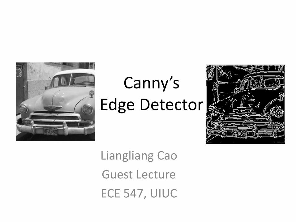
Canny’s Edge Detector
Liangliang Cao
Guest Lecture
ECE 547, UIUC
Reference
• John Canny’s paper: A Computational
Approach to Edge Detection, IEEE Trans
PAMI, 1986
• Peter Kovesi’s Matlab functions
http://www.csse.uwa.edu.au/~pk/Research/Matla
bFns/
Part I: Mathematical Model
Goal
• Canny's aim was to discover the optimal edge
detection algorithm:
– good detection – the algorithm should mark as
many real edges in the image as possible.
– good localization – edges marked should be as
close as possible to the edge in the real image.
– minimal response – a given edge in the image
should only be marked once, and where possible,
image noise should not create false edges.
Formulation
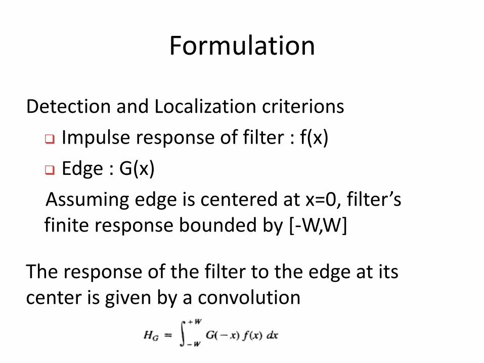
Detection and Localization criterions
Impulse response of filter : f(x)
Edge : G(x)
Assuming edge is centered at x=0, filter’s finite response bounded by [-W,W]
The response of the filter to the edge at its center is given by a convolution
Criterion 1: Signal/Noise Ratio
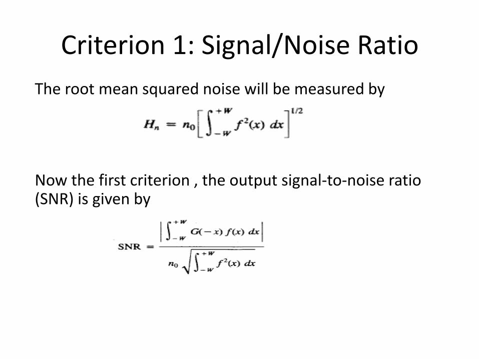
The root mean squared noise will be measured by
Now the first criterion , the output signal-to-noise ratio (SNR) is given by
Criterion 2: Localization
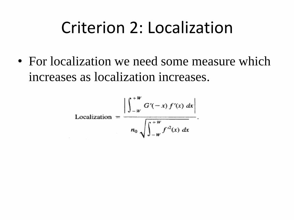
• For localization we need some measure which
increases as localization increases.
Criterion 3: Multiple Response
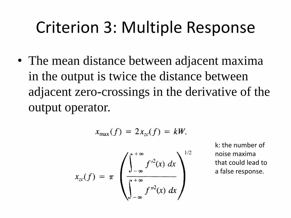
• The mean distance between adjacent maxima
in the output is twice the distance between
adjacent zero-crossings in the derivative of the
output operator.
k: the number of noise maxima that could lead to a false response.
General Optimization
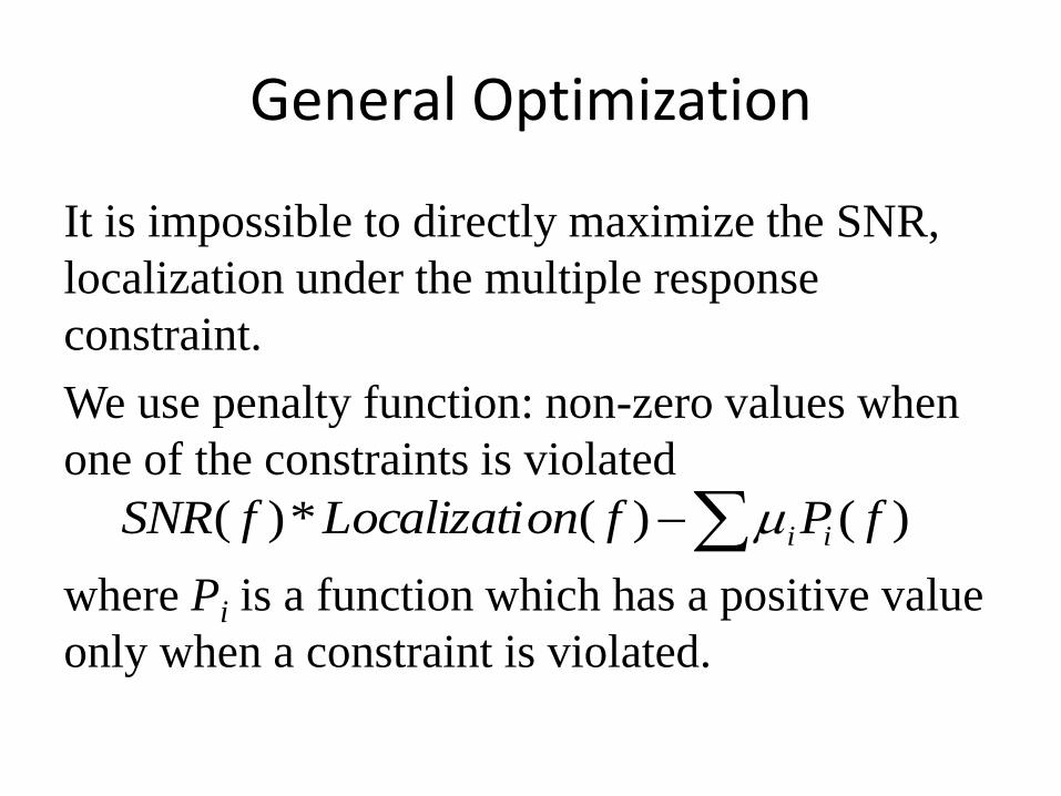
It is impossible to directly maximize the SNR,
localization under the multiple response
constraint.
We use penalty function: non-zero values when
one of the constraints is violated
where Pi is a function which has a positive value
only when a constraint is violated.
)()(*)( fPfonLocalizatifSNR ii
Optimization for special cases
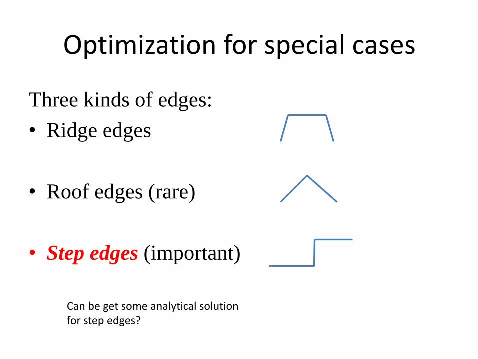
Three kinds of edges:
• Ridge edges
• Roof edges (rare)
• Step edges (important)
Can be get some analytical solution for step edges?
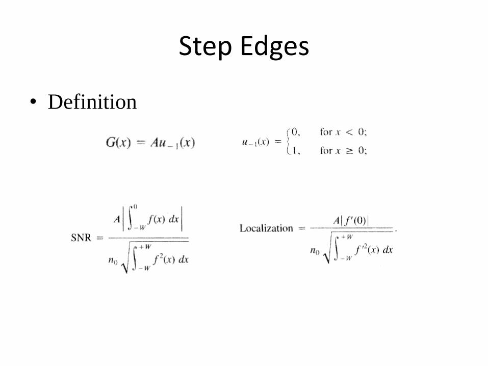
Step Edges
• Definition
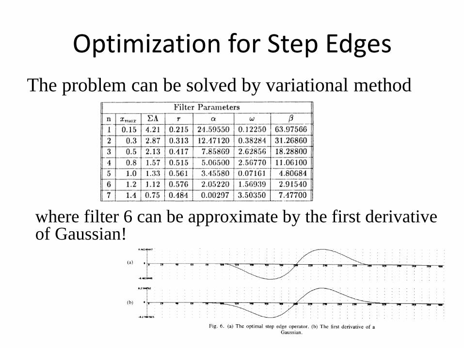
Optimization for Step Edges
The problem can be solved by variational method
where filter 6 can be approximate by the first derivative of Gaussian!
Summarization
• The type of linear operator that provides the
best compromise between noise immunity and
localization is First Derivative of Gaussian
• This operator corresponds to smoothing an
image with Gaussian function and then
computing the gradient

Part II: Implementation
Overview of Procedure
1) Smooth image with a Gaussian
2) Compute the Gradient magnitude using approximations of partial derivatives
3) Thin edges by applying non-maxima suppression to the gradient magnitude
4) Detect edges by double thresholding
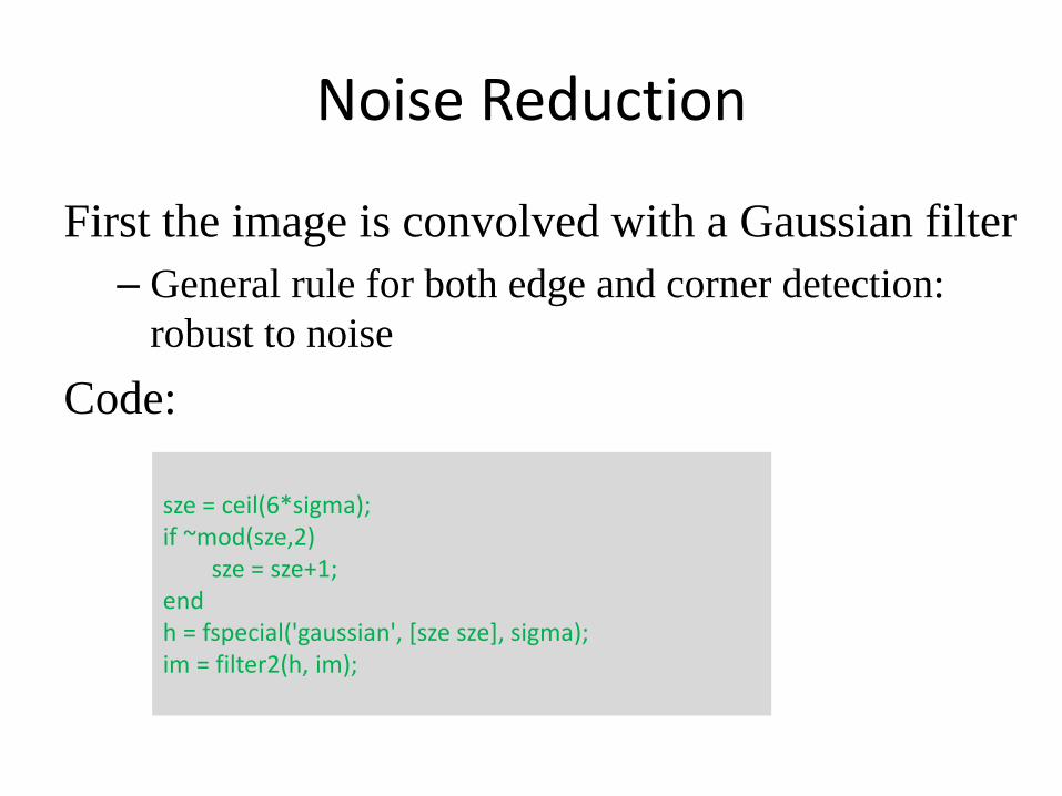
Noise Reduction
First the image is convolved with a Gaussian filter
– General rule for both edge and corner detection:
robust to noise
Code:
sze = ceil(6*sigma); if ~mod(sze,2) sze = sze+1; end h = fspecial('gaussian', [sze sze], sigma); im = filter2(h, im);
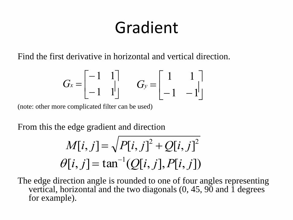
Gradient
Find the first derivative in horizontal and vertical direction.
(note: other more complicated filter can be used)
From this the edge gradient and direction
The edge direction angle is rounded to one of four angles representing vertical, horizontal and the two diagonals (0, 45, 90 and 1 degrees for example).
11
11xG
11
11yG
22 ],[],[],[ jiQjiPjiM
]),[],,[(tan],[ 1 jiPjiQji
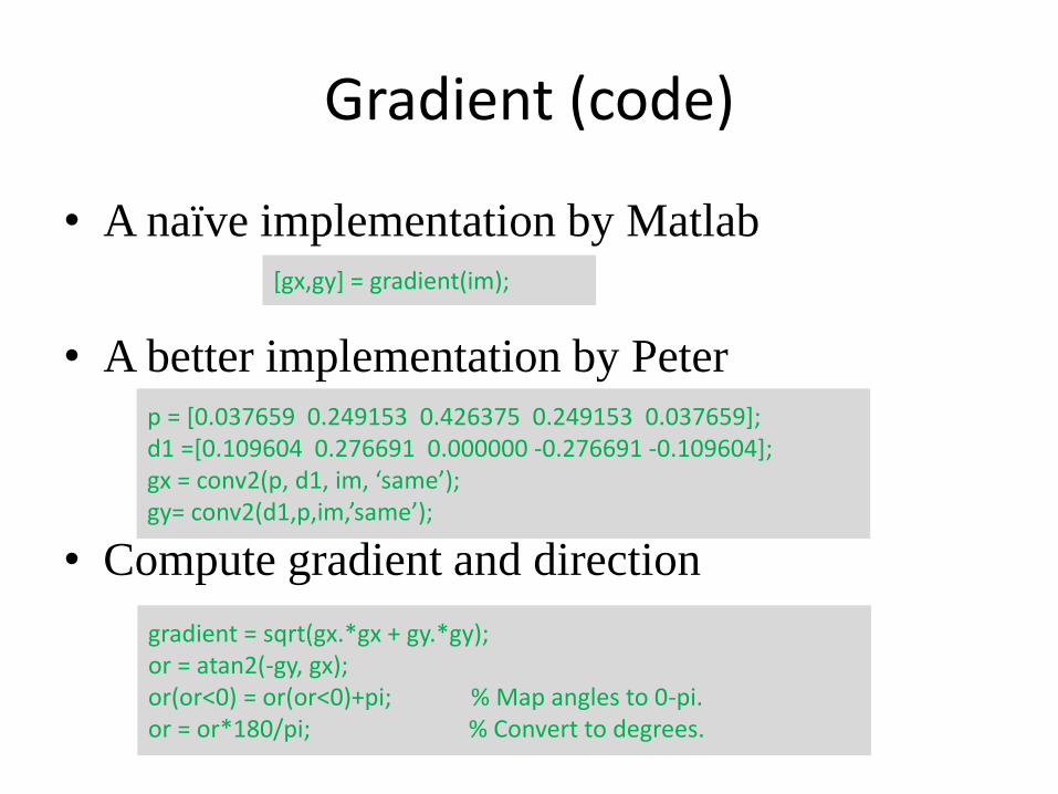
Gradient (code)
• A naïve implementation by Matlab
• A better implementation by Peter
• Compute gradient and direction
p = [0.037659 0.249153 0.426375 0.249153 0.037659]; d1 =[0.109604 0.276691 0.000000 -0.276691 -0.109604]; gx = conv2(p, d1, im, ‘same’); gy= conv2(d1,p,im,’same’);
[gx,gy] = gradient(im);
gradient = sqrt(gx.*gx + gy.*gy); or = atan2(-gy, gx); or(or<0) = or(or<0)+pi; % Map angles to 0-pi. or = or*180/pi; % Convert to degrees.
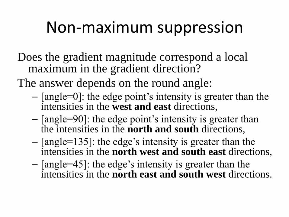
Non-maximum suppression
Does the gradient magnitude correspond a local maximum in the gradient direction?
The answer depends on the round angle: – [angle=0]: the edge point’s intensity is greater than the
intensities in the west and east directions,
– [angle=90]: the edge point’s intensity is greater than the intensities in the north and south directions,
– [angle=135]: the edge’s intensity is greater than the intensities in the north west and south east directions,
– [angle=45]: the edge’s intensity is greater than the intensities in the north east and south west directions.
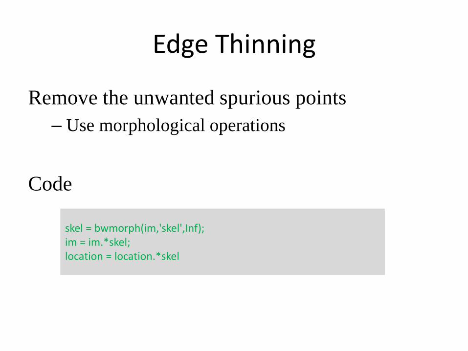
Edge Thinning
Remove the unwanted spurious points
– Use morphological operations
Code
skel = bwmorph(im,'skel',Inf); im = im.*skel; location = location.*skel
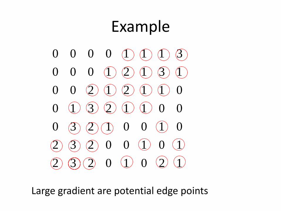
Example
Large gradient are potential edge points
12010232
10100232
01001230
00112310
01121200
13121000
31110000
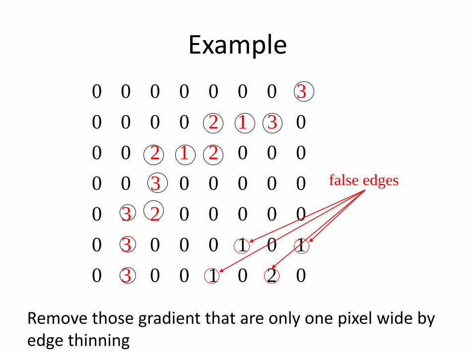
Example
0 2 0 1 0 0 3 0
1 0 1 0 0 0 3 0
0 0 0 0 0 2 3 0
0 0 0 0 0 3 0 0
0 0 0 2 1 2 0 0
0 3 1 2 0 0 0 0
3 0 0 0 0 0 0 0
false edges
Remove those gradient that are only one pixel wide by edge thinning
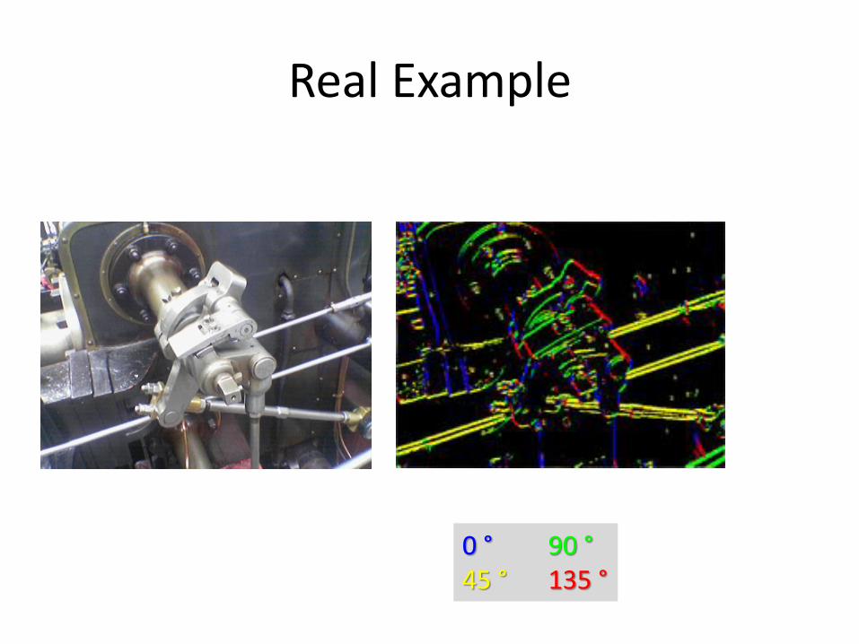
Real Example
0 ° 90 ° 45 ° 135 °
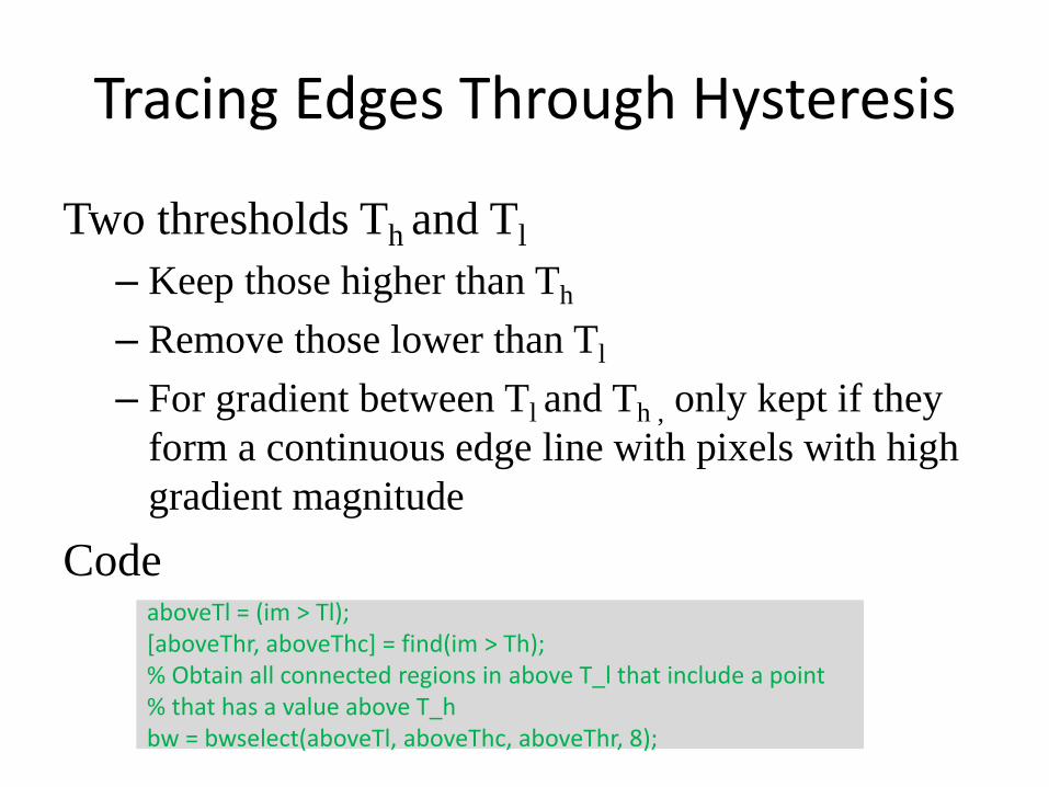
Tracing Edges Through Hysteresis
Two thresholds Th and Tl
– Keep those higher than Th
– Remove those lower than Tl
– For gradient between Tl and Th , only kept if they
form a continuous edge line with pixels with high
gradient magnitude
Code
aboveTl = (im > Tl); [aboveThr, aboveThc] = find(im > Th); % Obtain all connected regions in above T_l that include a point % that has a value above T_h bw = bwselect(aboveTl, aboveThc, aboveThr, 8);
25
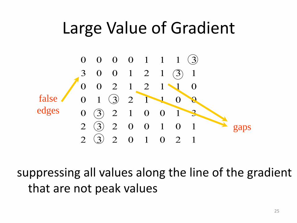
Large Value of Gradient
suppressing all values along the line of the gradient that are not peak values
12010232
10100232
31001230
00112310
01121200
13121003
31110000
gaps
false
edges
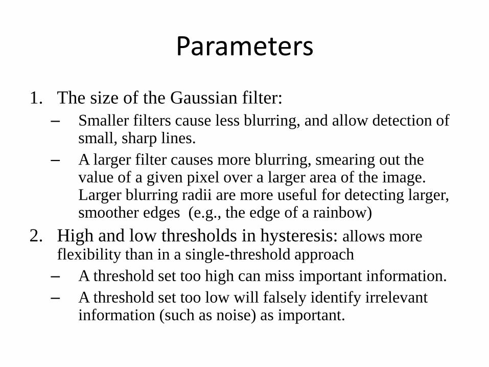
Parameters
1. The size of the Gaussian filter:
– Smaller filters cause less blurring, and allow detection of small, sharp lines.
– A larger filter causes more blurring, smearing out the value of a given pixel over a larger area of the image. Larger blurring radii are more useful for detecting larger, smoother edges (e.g., the edge of a rainbow)
2. High and low thresholds in hysteresis: allows more flexibility than in a single-threshold approach
– A threshold set too high can miss important information.
– A threshold set too low will falsely identify irrelevant information (such as noise) as important.
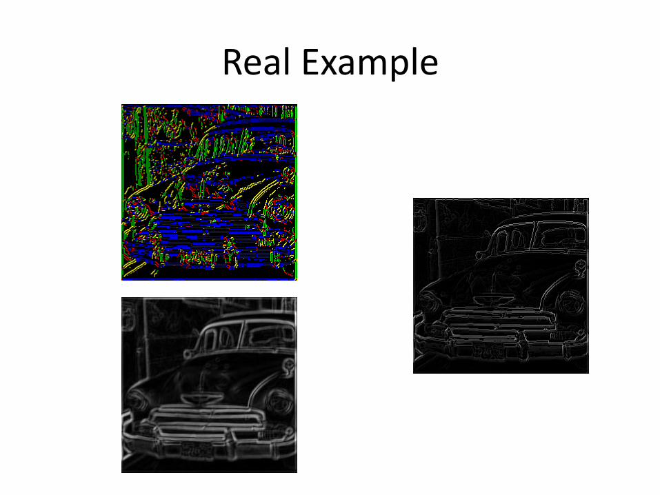
Real Example
Conclusion
• Canny edge detector has been still arguably the best edge detector for the last twenty years
• The operator of Gradient of Gaussian has rich theoretical meaning
• Beyond edges, corner detector is more popular in recent image recognition
– SIFT talked by Mert Dikmen


