
ISSN 2042-2695
CEP Discussion Paper No 1433
Revised October 2017 (Replaced June 2016 version)
Management as a Technology?
Nicholas Bloom Raffaella Sadun
John Van Reenen

Abstract Are some management practices akin to a technology that can explain firm and national productivity, or do they simply reflect contingent management styles? We collect data on core management practices from over 11,000 firms in 34 countries. We find large cross-country differences in the adoption of management practices, with the US having the highest size-weighted average management score. We present a formal model of \Management as a Technology", and structurally estimate it using panel data to recover parameters including the depreciation rate and adjustment costs of managerial capital (both found to be larger than for tangible non-managerial capital). Our model also predicts (i) a positive impact of management on firm performance; (ii) a positive relationship between product market competition and average management quality (part of which stems from the larger covariance between management with firm size as competition strengthens); and (iii) a rise in the level and a fall in the dispersion of management with firm age. We find strong empirical support for all of these predictions in our data. Finally, building on our model, we find that differences in management practices account for about 30% of total factor productivity differences both between countries and within countries across firms. Keywords: management practices, productivity, competition JEL Classifications: L2; M2; O32; O33 This paper was produced as part of the Centre’s Growth Programme. The Centre for Economic Performance is financed by the Economic and Social Research Council. Acknowledgements This project has received funding from the European Research Council (ERC) under the European Union’s Horizon 2020 research and innovation programme (Grant Agreement Number 670862).
We would like to thank Ufuk Ackigit, Orazio Attanasio, Marianne Bertrand, Robert Gibbons, John Haltiwanger, Rebecca Henderson, Bengt Holmström, Michael Peters, Michele Tertilt and Fabrizio Zilibotti for helpful comments as well as participants in seminars at the AEA, Barcelona, Berkeley, Birmingham, Bocconi, Brussels, CEU, Chicago, Dublin, Duke, Essex, George Washington, Harvard, Hong Kong, IIES, LBS, Leuven, LSE, Madrid, Mannheim, Michigan, Minnesota, MIT, Munich, Naples, NBER, NYU, Peterson, Princeton, Stockholm, Sussex, Toronto, Uppsala, USC, Yale and Zurich. The Economic and Social Research Council, the Kauffman Foundation, PEDL and the Alfred Sloan Foundation have given financial support. We received no funding from the global management consultancy firm (McKinsey) we worked with in developing the survey tool. Our partnership with Pedro Castro, Stephen Dorgan and John Dowdy has been particularly important in the development of the project. We are grateful to Renata Lemos and Daniela Scur for ongoing discussion and feedback on the paper. Anna Valero and Chiara Criscuolo have been generous in providing us with data. We thank Yo-Jud Cheng for excellent research assistance. Any opinions and conclusions expressed herein are those of the authors and do not necessarily represent the view of the U.S. Census Bureau. All results have been reviewed to ensure that no confidential information is disclosed. Nicholas Bloom, Stanford University and Centre for Economic Performance. Raffaella Sadun, Harvard University and Centre for Economic Performance. John Van Reenen, MIT and Centre for Economic Performance, London School of Economics. Published by Centre for Economic Performance London School of Economics and Political Science Houghton Street London WC2A 2AE All rights reserved. No part of this publication may be reproduced, stored in a retrieval system or transmitted in any form or by any means without the prior permission in writing of the publisher nor be issued to the public or circulated in any form other than that in which it is published. Requests for permission to reproduce any article or part of the Working Paper should be sent to the editor at the above address. N. Bloom, R. Sadun and J. Van Reenen, revised 2017.

1 Introduction
Productivity differences between firms and between countries remain startling. For example, within
the average four-digit U.S. manufacturing industries, Syverson (2011) finds that labor productivity
for plants at the 90thpercentile was four times as high as plants at the 10thpercentile. Even after
controlling for other factors, Total Factor Productivity (TFP) was almost twice as high. These
differences persist over time and are robust to controlling for plant-specific prices in homogeneous
goods industries.1 Such TFP heterogeneity is evident in all other countries where data is available.2
One explanation is that these persistent within industry productivity differentials are due to “hard”
technological innovations, as embodied in patents or the adoption of advanced equipment. Another
explanation, which is the focus of this paper, is that productivity differences reflect variations in
management practices.
We advance the idea that some forms of management practices are like a “technology”, in the
sense that they raise TFP. This has a number of empirical implications that we examine and find
support for in the data. Our perspective on management is distinct from the common “Design”
paradigm in organizational economics, which views management as a question of optimal design
depending on the very contingent features of a firm’s environment (Gibbons and Roberts, 2013).
In this view of management practices, there is no sense in which any management styles are on
average better than any others. Our data provides some support for Design perspective, but we
show that–at least within the very stylized version of this perspective that we consider–this delivers
only a partial explanation of the patterns that we can observe in our data.
To date, empirical work to measure differences in management practices across firms and countries
has been limited. Despite this lack of data, the core theories in many fields such as international
trade, labor economics, industrial organization and macroeconomics are now incorporating firm
heterogeneity as a central component.3
To address the lack of management data, we collect original survey data on management practices
on over 11,000 firms in 34 countries. Besides its rich cross sectional nature, both in terms of countries
and industries covered, this dataset also features a significant panel component built through four
1These are revenue based measures of TFP (“TFPR”) so will also reflect firm-specific mark-ups. Foster, Halti-wanger and Syverson (2008) show large differences in TFP even within very homogeneous goods industries such ascement and block ice where they can observe plant specific prices (“TFPQ”). In what follows we will refer simply toTFP acknowledging that empirical measures usually be TFPR. Konig, Lorenz and Zilibotti (2016) give an exampleof how these could reflect technology differences even for ex ante identical firms. Hall and Jones (1999) show howthe stark differences in productivity across countries account for a substantial fraction of the differences in averageincome.
2Usually productivity dispersion is even greater than in the U.S.–see Bartelsman, Haltiwanger and Scarpetta(2013), Hsieh and Klenow (2009) and OECD (2016).
3Different fields have different labels for what we regard as heterogeneity in management. In trade, the focus is onan initial productivity draw when the plant enters an industry that persists over time (e.g. Melitz, 2003). In industrialorganization, the focus has traditionally been on cost heterogeneity due to entrepreneurial/managerial talent (e.g.Lucas, 1978). In macro, organizational capital is sometimes related to the firm specific managerial know-how built upover time (e.g. Prescott and Visscher 1980). In labor, there is a growing focus on how the wage distribution requiresan understanding of the heterogeneity of firm productivity (e.g. Card, Heining and Kline, 2013).
2

different survey waves from 2004 to 2014. One purpose of this paper is to provide public use data
to enable other researchers to address long-standing questions regarding firm organization.4 We
first present some stylized facts from this database in the cross country and cross firm dimensions.
One of the striking features of the data is that the average management score, just like TFP, is
higher in the U.S. than it is in other countries (see Figure 1). A second striking feature is that
management, like TFP, shows a wide dispersion across firms within each country (see Figure 2).
Interestingly, this dispersion is lower in countries like the U.S., with lower levels of market frictions,
than it is in countries like India and Brazil.
We detail a simple model of “Management As a Technology” (MAT) which incorporates both
a heterogeneous initial draw of managerial ability when a firm starts up, and the endogenous
response of ongoing firms who change their level of managerial capital in response to shocks to
the environment (modeled as as idiosyncratic TFP shocks). The model is useful to formalize our
theoretical intuitions and enable structural estimation of key parameters. In particular, thanks
to the panel variation present in the management data, we are able to identify the depreciation
rate and adjustment costs of managerial capital, using Simulated Method of Moments (SMM). A
further benefit of the structural model is that it enables us to derive some additional predictions
on moments we did not target in the structural estimation.
We find that the data supports the predictions from the MAT model. First, management is pos-
itively associated with improved firm performance (productivity, profitability and survival) and,
from experimental evidence, the management effect appears to be causal. Second, firm manage-
ment rises with more intense product market competition, both through reallocating more economic
activity to the better managed firms (an Olley and Pakes (1996) covariance term), and also through
a higher unweighted average level of management. Third, older firms have a higher level of manage-
ment, but lower dispersion due to selection effects. We contrast our MAT model to the predictions
arising from a very stylized version of the “Management by Design” model, an alternative ap-
proach which sees management as a contingent feature, rather than an output-increasing factor of
production. There are some elements consistent with this second design approach, especially when
we disaggregate the management score into elements relating to monitoring compared relative to
incentives. However, overall the MAT model seems a better description of our data.
Finally, using our MAT model we show that on average just under a third of cross country TFP
differences with the U.S. are accounted for by management, with this fraction being higher in
OECD countries than in less developed nations. Thus, management practices can account for a
substantial portion of cross-country differences in development. Similarly when we look within
countries, about 30% of the 90-10 difference in productivity between firms is accounted for by
differences in management practices.
In summary, this paper makes three major contributions over the existing literature. First, it
4The methods and data are open source and available on our website http://worldmanagementsurvey.org/survey-data/download-data/.
3

develops and structurally estimates a model of management practices in the production function.
Second, it uses this model to determine the extent to which management can account for variations
in productivity across firms and across a large number of countries. Finally, it produces a set of
Public Use Micro Data which should facilitate future quantitative research in the area of managerial
and organizational economics.
Our paper relates to several literatures. First, there is a large body of empirical literature on the
importance of management for variations in firm and national productivity, going back to Walker
(1887) through to more recent papers like Ichniowski, Shaw and Prennushi (1997), Bertrand and
Schoar (2003), Adhvaryu, Kala and Nyshadham (2016) and Bruhn, Karlan and Schoar (2016).
Second, there is a growing macro literature on aggregate implications of firm management and
organizational structure, ranging from Lucas (1978), to Gennaioli et al (2013), Guner and Ventura
(2014), Garicano and Rossi-Hansberg (2015) and Akcigit, Alp and Peters (2016). Third, there
is a long literature on the causes of the slow diffusion of new technologies and the implications
for productivity differences (e.g. Griliches, 1957; Gancia, Mueller and Zilibotti, 2013). Finally,
there is another growing literature focusing on explaining cross-country TFP in terms of the degree
of reallocation of inputs to more productivity firms, most notably Hsieh and Klenow (2009) and
Restuccia and Rogerson (2008).
The structure of the paper is as follows. We first describe some theories of management (Section
2) and implements our structural approach. Section 3 describes the data and Section 4 details
our empirical results. Section 5 uses the framework to quantify the degree to which management
can account for the cross country and within country dispersion of productivity and Section 6
offers some concluding comments. The online Appendices describe the data and how it can be
accessed (A), further econometric analysis (B), details of the SMM procedure (C) and the CEO
compensation data (D).
2 Models of Management
2.1 Conventional approaches to modeling heterogeneity in firm productivity
Econometricians have often labeled the fixed effect in panel data estimates of production functions
“management ability”. For the most part, however, economists have focused on how technological
innovations influence growth; for example, correlating TFP with observable innovation indicators
such as Research and Development (R&D), patents, or information technology (IT). There is robust
evidence of the impact of such “hard” technologies for productivity growth (e.g. Griliches, 1998).
Nevertheless, there are at least two major problems in focusing on these aspects of technical change
as the sole driver of productivity. First, even after controlling for a wide range of observable
measures of hard technologies, a large residual in measured TFP still remains. Second, many
studies have found that the impact of technology on productivity varies widely across firms and
4

countries. In particular, information technology has much larger effects on the productivity of firms
that have complementary managerial structures which enable IT to be more efficiently exploited.5
Furthermore, a large body of case study work also suggests a major role for management in raising
firm performance (e.g. Baker and Gil, 2013).
In light of these issues, we believe it is worth directly considering management practices as an
independent factor in raising productivity.
2.2 Formal models of management
It is useful to analytically distinguish between two broad approaches that we can embed in a simple
production function framework where value added, Y, is produced as follows:
Y = F (A, L,K,M) (1)
where A is an efficiency term, labor is L, non-management capital is K, and M is management
capital.
We begin with the “Management as Technology” perspective, where some types of management (or
bundles of management practices) enhance productivity for the average firm across a wide range
of environments. There are three types of these “best practices”. First, there are some practices
that have always been better (e.g. not promoting incompetent employees to senior positions, or
collecting some information before making decisions). Second, there may be genuine managerial
process innovations (e.g. Taylor’s Scientific Management; Lean Manufacturing; Deming’s Total
Quality Management, etc.). Third, many management practices may have become optimal due to
changes in the economic environment over time. Incentive pay may be an example of this, as the
incidence of piece rates declined from the late 19th century, but appears to be making a comeback
today.6
The alternative framework is the more traditional approach in Organizational Economics which
we label the “Management by Design” perspective, where differences in practices are simply styles
optimized to a firm’s environment. For any indicator of M, such as the measures we gather,
the Design approach would not assume that output is monotonically increasing in M. In some
circumstances, higher levels of what we would regard as good practices will explicitly reduce output.
To take a simple example, consider M as a discrete variable which is equal to one if promotion takes
5In their case study of retail banking, for example, Autor et al (2002) found that banks who failed to re-organizethe physical and social relations within the workplace reaped little reward from their adoption of IT. More generally,Bresnahan, Brynjolfsson and Hitt (2002) found that decentralized organizations tended to enjoy a higher productivitypay-off from IT across a wide range of sectors. Similarly, Bloom, Sadun and Van Reenen (2012) found that ITproductivity was higher for firms with stronger incentives management, using some of the measures we detail belowin Section 3.
6Lemieux, MacLeod and Parent (2009) suggest that this may be due to advances in IT. Software companies likeSAP have made it much easier to measure output in a timely and robust fashion, making effective incentive payschemes easier to design and implement.
5
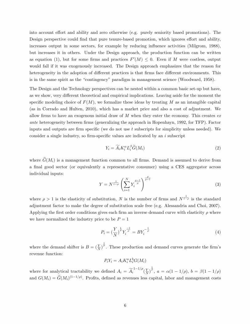
into account effort and ability and zero otherwise (e.g. purely seniority based promotions). The
Design perspective could find that pure tenure-based promotion, which ignores effort and ability,
increases output in some sectors, for example by reducing influence activities (Milgrom, 1988),
but increases it in others. Under the Design approach, the production function can be written
as equation (1), but for some firms and practices F ′(M) ≤ 0. Even if M were costless, output
would fall if it was exogenously increased. The Design approach emphasizes that the reason for
heterogeneity in the adoption of different practices is that firms face different environments. This
is in the same spirit as the “contingency” paradigm in management science (Woodward, 1958).
The Design and the Technology perspectives can be nested within a common basic set-up but have,
as we show, very different theoretical and empirical implications. Leaving aside for the moment the
specific modeling choice of F (M), we formalize these ideas by treating M as an intangible capital
(as in Corrado and Hulten, 2010), which has a market price and also a cost of adjustment. We
allow firms to have an exogenous initial draw of M when they enter the economy. This creates ex
ante heterogeneity between firms (generalizing the approach in Hopenhayn, 1992, for TFP). Factor
inputs and outputs are firm specific (we do not use t subscripts for simplicity unless needed). We
consider a single industry, so firm-specific values are indicated by an i subscript
Yi = AiKαi L
βi G(Mi) (2)
where G(Mi) is a management function common to all firms. Demand is assumed to derive from
a final good sector (or equivalently a representative consumer) using a CES aggregator across
individual inputs:
Y = N1
1−ρ
(N∑i=1
Yρ−1ρ
i
) ρρ−1
(3)
where ρ > 1 is the elasticity of substitution, N is the number of firms and N1
1−ρ is the standard
adjustment factor to make the degree of substitution scale free (e.g. Alessandria and Choi, 2007).
Applying the first order conditions gives each firm an inverse demand curve with elasticity ρ where
we have normalized the industry price to be P = 1
Pi = (Y
N)1ρY−1ρ
i = BY− 1ρ
i (4)
where the demand shifter is B = ( YN )1ρ. These production and demand curves generate the firm’s
revenue function:
PiYi = AiKai L
biG(Mi)
where for analytical tractability we defined Ai = Ai1−1/ρ
( YN )1ρ, a = α(1 − 1/ρ), b = β(1 − 1/ρ)
and G(Mi) = G(Mi)(1−1/ρ). Profits, defined as revenues less capital, labor and management costs
6

(cK(K), cL(L) and cM (M)), and fixed costs F are:7
Πi = AiKai L
biG(Mi)− cK(Ki)− cL(Li)− cM (Mi)− F
2.3 Models of management in production
In terms of the management function G(Mi), we consider two broad classes of models. First,
Management as a Technology where management is an intangible capital input in which output
is monotonically increasing. Second, Management by Design in which management is a choice of
production approach. We focus on the first as this fits the data better (as we show below), but lay
out both approaches in what follows.
2.3.1 Management as a Technology (MAT)
In Lucas (1978) or Melitz (2003) style models, firm performance is increasing continuously in
the level of managerial quality, which is synonymous with productivity. Firms draw a level of
management quality when they are born, and this continues with them throughout their lives.
Since these types of models assume G(Mi) is increasing in Mi, we simplify the revenue function by
assuming G(Mi) = M ci
PiYi = AiKai L
biM
ci (5)
More generally, we want to allow for the possibility that management can also be endogenously
improved; for example, by hiring management consultants, spending time developing or reinforcing
improved organizational processes (e.g. Toyota’s Kaizen meetings), or paying for a better CEO.
Although managerial capital can be improved in this way, failure to invest may mean it depreciates
over time like other tangible and intangible assets such as physical capital, R&D, and advertising.
Hence, we set up a more general model which still has initial heterogeneous draws of management
when firms enter, but treats management as an intangible capital stock with depreciation:
Mit = (1− δM )Mit−1 + IMit IMit ≥ 0 (6)
where IMit reflects investment in management practices, which has a non-negativity constraint
reflecting the fact that managerial capital cannot be sold. The physical capital accumulation
equation is similar except it allows for capital resale (at a cost which we discuss later).
Kit = (1− δK)Kit−1 + IKit (7)
7Since firms in our data are typically small in relation to their input and output markets, for tractability we ignoreany general equilibrium effects, taking all input prices (for capital, labor and management) as constant.
7

2.3.2 Management by Design
An alternative approach is to assume that management practices are contingent on a firm’s envi-
ronment, so that increases in M do not always increase output. In some sectors, high values of M
will increase output, and in others they will reduce output depending on the specific features of the
industry. We assume that optimal management practices may vary by industry and country, but
this could also occur across other characteristics like firm age, size, or growth rate. For example,
industries employing large numbers of highly skilled employees, like pharmaceuticals, will require
large investments in careful hiring, tying rewards to performance and monitoring output, while
low-tech industries can make do without these costly human resource practices. Likewise, optimal
management practices could vary by country if, for example, some cultures are more comfortable
with firing persistently under-performing employees (e.g. the U.S.) while others emphasize loyalty
to long-serving employees (e.g. Japan).
There are many ways to set up a Design model. As a simple example we define G(Mi) = 1/(1 +
θ|Mi −M |) where θ ≥ 0 and G(Mi) ∈ (0, 1] is decreasing in the absolute deviation of M from its
optimal level M.8 There are of course many other ways to model this idea, and our approach is
certainly not meant to represent the wide range of Design approaches, rather we see it as a simple
example to illustrate the implications of a G(Mi) function which attains an interior maximum.
2.3.3 Management as Capital?
We initially debated calling our main approach “Management as Capital” (rather than “Manage-
ment as a Technology”), viewing management as an intangible capital stock (see for example Bruhn,
Karlan and Schoar, 2016). In the end, because of the evidence suggesting management spillovers
across plants within firms and between different firms9 we thought modeling management as a tech-
nology seemed more appropriate. However, we recognize that either terminology could be used.
Indeed, the classic technology input–the R&D knowledge stock–is recorded as an intangible capital
input by the Bureau of Economic Activity in U.S. National Accounts.
2.4 Adjustment costs and dynamics
In general, changing a capital stock will involve adjustment costs. This could reflect, for example,
the costs of the organizational resistance to new management practices (e.g. Cyert and March, 1963,
or Atkin et al., 2017). We assume changing management practices involves a quadratic adjustment
cost:
CM (Mt,Mt−1) = γMMt−1(∆Mt
Mt−1− δM )2 −∆M
8Our baseline case also assumes that M is a choice variable that does not have to be paid for on an ongoing basisso that δM = 0 although this assumption is not material.
9For example, Greenstone, Hornbeck and Moretti (2010), Atalay, Hortascu and Syverson (2014), Braguinsky etal. (2015) and Bloom et al. (2017).
8

where the cost is proportional to the squared change in management net of depreciation, and scaled
by lagged management to avoid firms outgrowing adjustment costs. This style of adjustment costs is
common for capital (e.g. Chirinko, 1993) and seems reasonable for management where incremental
changes in practices are likely to meet less resistance than large changes. Likewise, we also assume
similar quadratic adjustment costs for non-managerial capital:
CK(Kt,Kt−1) = γKKt−1(Kt −Kt−1
Kt−1− δK)2 − It(1− φKD(It < 0))
where It is the investment rate, φK is the resale loss on capital and D(It < 0) is an indicator function
for disinvestment. To minimize on the number of state variables in the model, we assume labor is
costlessly adjustable, but requires a per period wage rate of w. Given this assumption on labor,
we can define the optimal choice of labor by ∂PY (A,K,L∗,M)∂L = w. Imposing this labor optimality
condition and assuming the MAT specification for management in the production function, we
obtain:
Y ∗(A,K,M) = A∗Ka
1−bMc
1−b
where A∗ = bb
1−bA1
1−b .10. Finally, ln(A) is assumed to follow a standard AR(1) process so that
ln(Ait) = lnA0 + ρAln(Ai,t−1) + σAεi,t where εi,t ∼ N(0, 1). This will generate the firm-specific
dynamics in the model, which alongside the random initial draw for management, which generate
the stochastics in our model.
2.5 Optimization and equilibrium
Given the firm’s three state variables–business conditions A, capital K, and management M–we
can write a value function (dropping i -subscripts for brevity):
V (At,Kt,Mt) = max[V c(At,Kt,Mt), 0]
V c(At,Kt,Mt) = maxKt+1,Mt+1
[Y ∗t − wL− CK(Kt+1,Kt)− CM (Mt+1,Mt)− F
+ rEtV (At+1,Kt+1,Mt+1)]
where the first maximum reflects the decision to continue in operation or exit (where exit occurs
when V c < 0, the value for “continuers”) , the V csecond is the optimization of capital and man-
agement conditional on operation, and r is the discount factor. We assume there is a continuum of
potential new entrants that would have to pay one period of fixed costs F to enter.11 Upon entry,
they take a stochastic draw of their productivity (A) and management (M ) from a known joint
distribution H(A,M) and start with non-managerial capital K0 = 0. Hence, entry occurs until the
10We define the units for labor, management and capital so that their prices are unity.11We can allow the entry sunk cost to be different from a one period fixed cost as in Bartelsman et al (2013). In
an earlier version of the paper we used firm level exit rates to estimate sunk costs and generated qualitatively resultsto those presented below. Since nothing in the results hinges on this, we kept the current set-up for simplicity.
9

point that the expected value of entry equals the sunk cost of entry:
F =
∫V (A, 0,M)dH(A,M)
We solve for the steady-state equilibrium by selecting the demand shifter (B = ( YN )1ρ) that ensures
that the expected cost of entry equals the expected value of entry given the optimal capital and
management decisions. This equilibrium is characterized by a distribution of firms in terms of their
state values A,K,M . The distribution of lnA is assumed normal, while M is assumed to be drawn
from a uniform distribution.12
2.6 Numerical Estimation
Appendix C discusses this in more detail. In short, solving the model requires finding two nested
fixed-points.13 First, we solve for the value functions for incumbent firms using the contraction
mapping (e.g. Stokey and Lucas, 1986), taking demand as given for each firm. The policy cor-
respondences for M and K are formed from the optimal choices given these value functions, and
for L from the static first-order condition. Second, we then iterate over the demand curve (3) to
satisfy the zero-profit condition.14 Once both fixed points are satisfied, we simulate data for 5,000
firms over 50 years to get to an ergodic steady-state, and then discard the first 40 periods to keep
the last 10 years of data (to match the time span of our management panel data).
To solve and simulate this model we also need to define a set of 14 parameter values. We pre-define
nine of these from from accounting measurement (e.g. the labor share of GDP, the depreciation rate
on capital) or estimates in the prior literature, we normalize two (fixed costs to 100 and the mean
of ln(TFP) to 1) and estimate the remaining three parameters on our management and accounting
data panel. The nine predefined parameters are listed in Table 1, and are all based on standard
values in the literature. Appendix C describes how we cross-checked these calibration values with
our own WMS data. For example, the Cooper and Haltiwanger (2006) estimates of the standard
deviation (σA) and auto-correlation of TFP (ρA) implicitly include managerial capital (M), which
we can observe in our data. The three unknown parameters that we choose to estimate are those
where much less is known from the literature. The adjustment cost (γM ) and depreciation rates
(δK) for management have never been estimated before, to our knowledge. We also estimate the
adjustment cost for non-managerial capital (γK). While prior papers have estimated labor and
capital adjustment costs (e.g. Bloom, 2009, and the survey therein), they have typically ignored
management as an input, so it is these parameters are not directly transferable to our set-up.
12Nothing fundamental hinges on the exact distributional assumptions for M and A.13The full replication package for the simulation and SMM estimation is available on
http://web.stanford.edu/˜nbloom/MAT.zip
14If there is positive expected profit then net entry occurs and the demand shifter B = ( YN
)1ρ
falls, and if there isnegative expected profit then net exit occurs.
10

To estimate the model by SMM we picked three data moments to match: the variance of the five-
year growth rates of the three state variables (management capital, non-management capital, and
TFP) to tie down the adjustment cost and depreciation parameters. These data moments were
generated on the matched management-accounting panel dataset for all countries from 2004 to 2014
(described in more detail in the next section). To generate standard errors, we block-bootstrapped
over firms the entire process 1,000 times to generate the variance-covariance matrix, which was also
used to optimally weight the SMM criterion function.
2.7 Simulation results
The top panel of Table 2 contains the SMM estimates and standard errors values for the three
estimated parameters, and the bottom panel contains the moments from the data used to estimate
these. Because the model is exactly identified we can precisely match the moments within numerical
rounding errors.
The estimation of the adjustment costs for management is one of the novel contributions of this
paper. We obtain a slightly higher level of adjustment costs for management of 0.212 (compared
to 0.195 for capital) which, alongside the irreversibility of management, helps generate smoother
management five-year growth moments compared to capital five-year growth moments (see the
bottom panel of Table 2).15 These magnitudes are prima facie plausible as prior research in this
area (Cyert and March, 1963) and anecdotal evidence from the private equity and management
consulting industry suggest that management practices are likely to as hard or even harder to
change than plant or equipment (e.g. Davis et al, 2014). Depreciation of management capital is
12.9%, similar to the level of the depreciation of capital (10%, see Table 1).16
Having defined and estimated the main MAT model, we can proceed to examine covariances of
various moments that we have not targeted in the structural estimation to later compare these
with actual data. Figures 3 through 5 show some predictions arising from the simulation. In
Figure 3, we start by comparing the distribution of management practices of a random draw of
15,489 firm-years from our simulation to the 15,489 firm-year surveys in the management panel
data, revealing similar cross-sectional distributions.17 While this is not a formal test of our model,
it does confirm it can generate the wide spread of management practices, that is a striking finding
of the management survey data.
15If we allow management to be have the same 50% resale loss as capital its adjustment cost is estimated to be0.290, about 50% higher than the value for capital.
16One interpretation is that management capital is tied to the the identity of plant managers. The average jobtenure for plant managers in our survey is 6.4 year in the post and and 13.0 years in the company, which would implypost and company quit rates of about 15% to 7% spanning the depreciation estimate of 13%. Indeed, in the 8-yearfollow-up to the Bloom et al. (2013) India experiment the largest reasons for a deterioration in management practicesin the treatment plants was the attrition of the plant manager.
17To scale our management practices we take logs of the management variable, and normalize the lowest value to1 and the higher value to 5 to replicate our management survey scoring tool.
11

Figure 4 examines the relationship between management and product market competition as in-
dexed by the elasticity of demand (ρ). We run all the simulation for increasingly high levels of the
absolute price elasticity of demand between three and fifteen (recall that our baseline is an elasticity
is equal to five). This represents economies with increasingly high levels of competition. We see
that average management scores are higher when competition is stronger. The darker bars are the
unweighted means of management across firms–they rise because under higher competition poorly
managed firms tend to exit, as they cannot cover their fixed cost of production. We also see that
size (employment) weighted management practices rise even faster with competition, because this
raises the covariance between firm size and management (a higher “Olley Pakes reallocation” term),
as better managed firms acquire larger market shares (and therefore need more inputs). Finally,
Figure 5 examines the relationship between management and firm age. Firms’ management score
rises with age, as poorly managed firms either improve or exit the market. Over time, this leads
the dispersion of management practices to fall within any age cohort, because of the exit of poorly
managed firms.
Panels A to C of Figure 6 provide similar figures to Figures 3 to 5 for our Management by Design
model, in which we assume G(M) is maximized at M = 3 for illustrative purposes. In Panel
A, we see a similar spread of management practices, suggesting the Design view can generate an
equilibrium dispersion of management practices. But in Panel B we see a very different relationship
with competition, where management practices are invariant with the level of competition. More
specifically, there is no sense in which high levels of management are better, and therefore they
are not positively selected as competition increases. In Panel C, we also see no variation in the
average management score with age for similar reasons, although we do see some reduction in
variance with age as extremely high and low values of management practices are modified or the
firm exits. Finally, in Panel D we have also included a plot of performance in terms of sales against
management, showing the inverted U shape implied by the Design view of the world that firms
have an optimizing level of M at 3.
3 Data
3.1 WMS Survey method
We describe the datasets in more detail in Appendix A, but sketch out the important features
here. To measure management practices, we developed a survey methodology known as the World
Management Survey (WMS).18 This uses an interview-based evaluation tool that defines 18 basic
management practices and scores them from one (“worst practice”) to five (“best practice”) on a
scoring grid. This evaluation tool was first developed by an international consulting firm, and scores
18More details can be found at http://worldmanagementsurvey.org/
12

these practices in three broad areas.19 First, Monitoring : how well do companies track what goes on
inside their firms, and use this for continuous improvement? Second, Target setting : do companies
set the right targets, track outcomes, and take appropriate action if the two are inconsistent?
Third, Incentives/people management20: are companies promoting and rewarding employees based
on performance, and systematically trying to hire and retain their best employees?
To obtain accurate responses from firms, we interview production plant managers using a “double-
blind” technique. One part of this technique is that managers are not told in advance they are
being scored or shown the scoring grid. They are informed only that they are being “interviewed
about management practices for a piece of work”. The other side of the double blind technique is
that the interviewers do not know anything about the performance of the firm.
To run this blind scoring, we used “open” questions. For example, on the first monitoring question
we start by asking the open question, “tell me how your monitor your production process”, rather
than closed questions such as “Do you monitor your production daily? [yes/no]”. We continue
with open questions focused on actual practices and examples until the interviewer can make an
accurate assessment of the firm’s practices. For example, the second question on that performance
tracking dimension is, “What kinds of measures would you use to track performance?” and the
third is “If I walked around your factory, could I tell how each person was performing?”.21
The other side of the double-blind technique is that interviewers are not told anything about the
firm’s performance in advance. They are only provided with the company name, telephone number,
and industry. Since we randomly sample medium-sized manufacturing firms (employing between
50 and 5,000 workers) who are not usually reported in the business press, the interviewers will
generally have not heard of these firms before, so they should have few preconceptions.22
The survey was targeted at plant managers, who are senior enough to have an overview of manage-
ment practices but not so senior as to be detached from day-to-day operations. We also collected
a series of “noise controls” on the interview process itself–such as the time of day, day of the week,
characteristics of the interviewee, and the identity of the interviewer. Including these in our re-
gression analysis typically helps to improve our estimation precision by stripping out some of the
random measurement error.
To ensure high sample response rates and informative interviews, we hired students with some
19Bertrand and Schoar (2003) focus on the characteristics and style of the CEO and CFO, and more specifically ondifferences in strategic management (e.g. decision making applied to mergers and acquisitions), while Lazear, Shawand Stanton (2016) focus on individual supervisors. The type of practices we analyze in this paper are closer tooperational and human resource practices, which has a long precedent in the management and strategy literature–forexample, Osterman (1994), Huselid (1995) and Capelli and Neumark (2001).
20These practices are similar to those emphasized in earlier work on management practices, by for example Ich-niowski, Prennushi and Shaw (1997) .
21The full list of questions for the grid is in Table A1 and (with more examples) athttp://worldmanagementsurvey.org/wp-content/images/2010/09/Manufacturing-Survey-Instrument.pdf.
22We focus on firms over a size threshold because the formal management practices we consider are likely to beless important for smaller firms. We had a maximum size threshold because we only interviewed one or two plantmanagers in each firm, so would have too incomplete a picture for very large firms. Below, we show tests suggestingour results are not biased by using this sampling scheme (see Appendix B).
13

business experience and training. We obtained endorsements from respected institutions for the
surveys in each country we covered. We also never asked interviewees for financial data, obtaining
this instead from independent sources on company accounts. Finally, the interviewers were encour-
aged to be persistent–so they ran about two interviews a day lasting 45 minutes each on average,
with the rest of the time (about 6 hours a day) spent repeatedly contacting managers to schedule
interviews. This process, while time consuming and expensive, helped to yield a 41% response rate
which was uncorrelated with the (independently collected) performance measures. Appendices A
and B discuss and analyze selection issues for the sampling frame and responders.
3.2 Survey waves
We have administered the survey in several waves since 2004. There were five major waves in
2004, 2006, 2009/10, 2013, and 2014. In 2004 we surveyed four countries (France, Germany, the
U.K. and the U.S.). In 2006 we expanded this to twelve countries (including Brazil, China, India,
and Japan), continuing random sampling, but in addition to a refreshment sample for the 2004
countries we also re-contacted all of the original 2004 firms to establish a panel. In 2009/10 we
re-contacted all the firms surveyed in 2004 and 2006, but did not do a refreshment sample (due to
budgetary constraints). In 2013 we added an additional number of countries (mainly in Africa and
Latin America). In 2014 we again did a refreshment sample, but also followed up the panel firms
in the U.S. and some E.U. countries. The final sample includes 34 countries and a panel of up to
four different years between 2004 and 2014 for some firms. In the full dataset we have 11,383 firms
and 15,489 interviews where we have usable management information.
3.3 Internal validation
We re-surveyed a random sub-sample of firms using a second interviewer to independently survey
a second plant manager in the same firm. The idea is that the two independent management
interviews on different plants within the same firms reveal how consistently we are measuring
management practices. We found that in this sample of 222 re-rater interviews, the correlation
between our independently run first and second interview scores was 0.51 (p-value 0.001). Part of
this difference across plants within the same firm is likely to be real internal variation in management
practices, with the rest presumably reflecting survey measurement error. The highly significant
correlation across the two interviews suggests that while our management score is clearly noisy, it
is picking up significant management differences across firms.
3.4 Some descriptive statistics
The bar chart in Figure 1 that we referred to in the Introduction plots the average (unweighted)
management practice score across countries. This shows that the U.S. has the highest average
14

management practice score, with the Germans, Japanese, Swedes, and Canadians below, followed
by a block of West European countries (e.g. France, Italy and the U.K.) and Australia. Below
this group is Southern European countries (e.g. Portugal and Greece) and Poland. Emerging
economies (e.g. Brazil, China, and India) are next, and low income countries (mainly in Africa)
are at the bottom. In one sense this cross-country ranking is not surprising since it approximates
the cross-country productivity ranking. But the correlation is far from perfect –Southern European
countries do a lot worse than expected and other nations, like Poland and Mexico, do better.23
A key question is whether management practices are uniformly better in some countries like the
U.S. compared to India, or if differences in the shape of the distribution drive the averages? Figure
2 plots the firm-level histogram of management practices (solid bars) for all countries pooled (top
left) and then for each country individually. This shows that management practices, just like firm-
level productivity, display tremendous variation within countries. Of the total firm-level variation
in management only 13% is explained by country of firm location, a further 10% by industry
(measured at the three digit SIC level), with the remaining 77% being within country and industry.
Interestingly, countries like Brazil and India have a far larger left tail of management (e.g. scores
of two or less) than the U.S. 24 This immediately suggests that one reason for the better average
performance in the U.S. is that the American economy is better at selecting out the badly managed
firms. We pursue the idea that some of the U.S. advantage may be linked to stronger forces of
competition below.
Figure A1 shows average management scores in domestic firms (i.e. those who are not part of
groups with overseas plants) compared to plants belonging to foreign subsidiaries. The average
scores in domestic plants look similar to those in Figure 1, which is unsurprising as most of our firms
are domestic. More interesting is that plants belonging to foreign multinationals appear to score
highly in almost every country, suggesting that such firms are able to transplant their management
practices internationally. This finding is robust to controlling for many other factors (such as firm
size, age and industry) and is consistent with the idea of a subset of global, productivity enhancing
practices. An interesting extension to our basic model would be to allow for this type of cross-plant
transfer of management practices (e.g. Helpman, Melitz and Yeaple, 2004) but for parsimony in
the current model we have not done so.
3.5 Managerial and Organizational Practices Survey (MOPS)
We also implemented a more traditional closed question “tick box” survey design for MOPS which
gives us management data on 31,793 U.S. manufacturing plants in 2010. The question design was
modeled on WMS and the response to the MOPS was very high as we worked with the U.S and
replies were legally mandatory. Census Bureau. Details on MOPS is contained in Bloom et al
23Polish management appears to be better because of the influence of the large numbers of German multinationalsubsidiaries, while Mexico similarly benefits from a heavy U.S. multinational presence
24For example, the skewness of the firm level management distribution in the U.S. is 0.09, whereas the skewness ofthe distribution in Brazil is 0.16 and 0.36 in India.
15

(2017) and Appendix A. One advantage of MOPS is that it has much more reliable information on
plant and firm age than in WMS –as discussed in later sections of this paper–so we use MOPS for
one of our theoretical predictions on the relationship between management and age.
4 Implications of Management as a Technology
4.1 Management and firm performance
Basic results
The most obvious implication of the MAT model is that high management scores should be asso-
ciated with better firm performance. Figure A2 plots firm sales on firm management and Figure
A3 does the same for conventionally measured firm TFP and management scores using local linear
regressions. Both figures show a clear positive and monotonic relationship. To probe this bivariate
relationship more formally, we run some simple regressions. We z-score each individual practice,
average across all 18 questions, and z-scored this average so the management index has a stan-
dard deviation of unity.25 Table 3 examines the correlation between different measures of firm
performance and management. To measure firm performance we used company accounts data26,
estimating production functions where Qit is measured by the value added of firm i at time t :
lnQit = αMMit + αLlnLit + αK lnKit + αXxit + uit (8)
where Mit is the empirical management score27, xit is a vector of other controls such as the pro-
portion of employees with a college degree, firm age, noise controls (e.g. interviewer dummies),
country and three-digit SIC industry dummies and uit is an error term. In column (1) of Table 3
we regress ln(value added) on ln(employment) and the management score, finding a highly signifi-
cant coefficient of 0.316. This suggests that firms with one standard deviation of the management
score are associated with 32 log points higher labor productivity (i.e. about 37%). In column (2)
we add the capital stock and other controls which causes the coefficient on management to drop to
0.148, although it remains significant. Column (3) conditions on a sub-sample where we observe
each firm in at least two years to show the effects are stable, while column (4) re-estimates the
25We have experimented with other ways of aggregating the management scores such as using principal componentanalysis. Since the 18 questions are all positively correlated these more sophisticated alternatives produce broadlysimilar results to those developed here. Sub-section 4.5 below describes some other ways of dis-aggregating the scoresinto sub-components that reveals evidence for the Design perspective.
26Our sampling frame contained 90% private firms and 10% publicly listed firms. In most OECD countries bothpublic and private firms publish basic accounts. In the U.S., Canada and India, however, private firms do not publish(sufficiently detailed) accounts so no performance data is available. Hence, these performance regressions use datafor all firms except privately held ones in the U.S., Canada and India.
27Note that empirical measure of management here, M, corresponds to the log of the managerial capital stock (lnM )in the theory. This seems reasonable given the evidence of Figure 3 of the log-normal distribution of the empiricalscore.
16
specification on this sub-sample including a full set of firm fixed effects to identify from changes in
management over time, a very tough test given the likelihood of attenuation bias. The coefficient
on management (and labor and capital) does fall, but it remains positive and significant.28 In
column (5) we use the Olley and Pakes (1996) estimator of productivity and obtain a coefficient on
management of 0.102, lying between the levels OLS and fixed effects specification.29
As discussed above, one of the most basic predictions is that better managed firms should be larger
than poorly managed firms. Column (6) of Table 3 shows that better managed firms are significantly
larger than poorly managed firms: a one standard deviation of management is associated with a 40
log point increase in employment size. In column (7) we use profitability as the dependent variable
as measured by ROCE (Return on Capital Employed) and show again a positive association with
management. Considering more dynamic measures, column (8) uses sales growth as a dependent
variable, revealing that better managed firms are significantly more likely to grow. Column (9)
estimates a model with Tobin’s average q as the dependent variable, which is a forward looking
measure of performance. Although this can only be implemented for the publicly listed firms, we see
again a positive and significant association with this stock market based measure. Finally, column
(10) examines bankruptcy/death and finds that better managed firms are significantly more likely
to survive.
These are conditional correlations that are consistent with the MAT model, but are obviously not
to be taken as causal. However, the randomized control trial (RCT) evidence in Indian textile
firms (Bloom et al, 2013) showed that increasing WMS style management scores by one standard
deviation in management caused a 10% increase in TFP. This estimate is consistent with the Olley-
Pakes in column (5) of Table 3. Other well identified estimates of the causal impact of management
practices such as the RCT evidence from Mexico discussed in Bruhn, Karlan and Schoar (2016) and
the management assistance natural experiment from the Marshall plan discussed in Giorcelli (2016)
find similarly large impacts of management practices on firm productivity (see also the literature
surveys by McKenzie and Woodruff, 2013, 2017, on smaller firms).
4.2 Product Market Competition
4.2.1 Competition and management
An important implication of the management as technology model is that stronger product market
competition is likely to improve average management scores. To test this prediction, we estimate
28Note that these correlations are not simply driven by the “Anglo-Saxon” countries, as one might suspect if themanagement measures were culturally biased. We cannot reject that the coefficient on management is the same acrossall countries: the F-test (p-value) on the inclusion of a full set of management*country dummies is 0.790 (0.642).
29In Appendix B1 and Table A5 we discuss a variety of other robustness tests of these productivity equations suchas using an output rather than value added production function and including materials as an additional input; usingthe System-GMM approach of Blundell and Bond (2000) as well as alternative control function approaches to Olley-Pakes as discussed by Ackerberg, Caves and Frazer (2015); using a Solow-residual based measure of conventionalTFP and using the wage bill instead of employment as a measure of labor services. The importance of managementremained in all of these experiments.
17

regressions of the form:
Micjt = γ1COMPETITIONcjt + γ2zit + ηt + ξcj + νicjt (9)
where zit is a vector of other firm controls (the proportion of employees with a college degree, log
firm and plant size, log firm age and noise controls), ηt denotes year dummies, ξct denotes a full set
of three digit SIC industry dummies by country, and v is an error term.
We employ three different industry measures of competition. First, we begin with the inverse
industry Lerner index measured in an industry by country by period cell. The Lerner index is
a classic measure of competition (Aghion et al, 2005), and is calculated as the median price cost
margin within an industry-country cell using all firms in the ORBIS accounting database.30 Since
profits data is not generally reported for firms in developing countries, we focus on OECD countries.
We build a time varying Lerner index using data relative to three different periods (2003-2006; 2008-
2011; 2012-2013).31 These industry by country by period variables are then correlated with the
management scores conducted over the same time periods.
As an alternative to the Lerner measure of competition, we use a measure of import penetration
(imports over apparent consumption) in the country by industry by period cell, again measured
in the same periods and for the same set of OECD countries using industry by country by year
data from the World Input-Output Database (WIOD). Finally, to take into account the fact that
observed changes in import competition may be endogenous, we build an alternative measure of
import penetration from WIOD which includes only imports from China, as these have been shown
in other papers (e.g. Autor, Dorn and Hansen (2013) and Bloom, Draca and Van Reenen, 2016)
to be overwhelmingly driven by policy changes such as Chinese accession to the WTO and the
subsequent reduction in tariffs and quotas (e.g. the dismantling of the Multi-Fiber Agreement).
We begin by just showing the raw data in Figure 7, binning the three competition measures into
terciles and plotting the mean management score in each bin. Panel A shows this for cross sec-
tional “levels” (after subtracting the overall industry means and overall country means in both the
competition measure and the management score), revealing a robustly positively relationship for all
three competition measures. Panel B reports a similar graphic for “changes” in management over
time within a country by industry pair (i.e. subtracting the country by industry means) against
changes in competition over time, again displaying a robustly positive relationship.
In Table 4, we examine this more formally in a regression context estimating equation (5). The
dependent variable across all columns is the standardized value of the management score. Column
30In the simulated data we confirm that this empirical measure of the Lerner Index is highly correlated with ourconsumer price sensitivity parameter, ρ. For example, the Lerner has a correlation of 0.928 with price sensitivityacross simulations in which we increase ρ in unit increments from 3 to 15.
31See the Appendix for details on the construction of the measures of competition. These roughly correspond toblocks of time before, during and after the Great Recession/Euro Crisis. 2013 is the last full year of the ORBISdatabase currently available.
18

(1) reports the correlation between management and competition including industry by country
fixed effects, time dummies and other standard firm-level controls. Consistent with Figure 7, the
Lerner Index has a positive and significant correlation with management. The simulation model
suggests that this relationship should be stronger if we size-weight management due to better
reallocation in more competitive sectors. Column (2) implements this idea using as a weight the
firm’s share of employment in the industry by country cell, and indeed, the coefficient on the Lerner
measure rises from 0.99 to 1.75. The next four columns repeat the specifications but use import
penetration, including imports from all countries in columns (3) and (4) and then just imports from
China in columns (5) and (6), as an alternative measure of competition. The pattern of results
shows a larger coefficient on the competition measures for the size-weighted regressions compared
to the unweighted regressions, consistent with the findings from using the Lerner index.32
Overall, the results suggest that higher competition is associated with significant improvements in
management, and the magnitude of the coefficient is larger when we weight the regressions by firm
size. In terms of magnitudes a one standard deviation change in the Lerner index in the unweighted
regression is associated with a 0.06 of a standard deviation change in management, compared to
0.02 using the import penetration measure and 0.05 using Chinese imports. The equivalent numbers
for the weighted regressions are 0.11, 0.05 and 0.05.33
4.2.2 Competition and reallocation towards better managed firms
Another way to confirm the reallocative impact of competition predicted by the MAT model is
to consider whether factors that reduce the degree of competition reduce the covariance between
management practices and firm size, implying δ1 < 0 in the following equation:
FirmSizeit = δ1 (M ∗ COMPETITION)it + δ2Mit + δ3COMPETITION i + δ4xijt + νijt (10)
The simplest method of testing this idea is to use countries grouped into regions to proxy competi-
tive frictions, as it is likely that competition is stronger in some regions (e.g. the U.S.) than others
(e.g. southern Europe).
32We also considered a fourth measure of competition from our survey data: the number of rivals as perceived bythe plant manager. The advantage of this indicator is that it is available for all countries in our survey. Empirically,the variable is also linked to improvements in management. In a specification like column (1) of Table 4, the coefficient(standard error) on this measure of competition was 0.033 (0.017) on a sample of 14,305 observations including allcountries with management data, and 0.059 (0.022) on the sample of OECD countries overlapping with the one usedin Table 4 (8,414 observations as there are a few some missing values on the number of competitors variable). Thedisadvantage of the number of rivals measure is that it is not tightly linked to the theory simulations. For example,although falls in barriers to entry will tend to increase the number of firms in the MAT model, increases in consumersensitivity to price can lead to an equilibrium reduction in the number of firms.
33To check whether the difference between the weighted and the unweighted results was significant, we comparedthe distribution of the estimated coefficients with and without weights bootstrapping with 500 replications. Theweighted coefficients were larger than the unweighted coefficients 84% of the times for the Lerner index, 76% of thetimes with the import penetration variable, and 52% of the times using imports from China.
19

Column (1) of Table 5 reports the results of a regression of firm employment on the average
management score and a set of industry, year and country dummies.34 The results indicate that
increasing a firm’s management score by one standard deviation is associated with an extra 183
workers. In column (2) we allow the management coefficient to vary by region, with the U.S. as the
omitted base. The negative coefficients on the interactions indicate that that there is a stronger
relationship between size and management in the U.S. compared to other regions. This difference
is significant for Africa, Latin America and southern Europe, but not for Asia or northern Europe.
A one standard deviation increase in management is associated with 268 extra employees in the
U.S. but only 68 (= 268.4 - 199.5) extra workers in southern Europe.35 These results suggest that
reallocation is stronger in the U.S. than in the other countries, which is consistent with the findings
on productivity in Bartelsman, Haltiwanger and Scarpetta (2013) and Hsieh and Klenow (2009).
We also investigate explicit measures of market-friction variables that can reduce competition. In
columns (3) to (5) of Table 5 we use country-wide measures of employment regulation from the
OECD and trade costs from the World Bank. Both of these reduce the covariance between firm size
and management practices. Finally in column (6) we use the more detailed country by industry
measures of tariffs from Feenstra and Romalis (2012) in deviations from their country and industry
mean, and again find a significant negative interaction. This implies that within a sector (like
steel), countries with higher tariffs (such as Brazil) will allocate less activity to better managed
firms than those with lower tariffs (such as the U.K.).
Taken as a whole, these findings on competition appear very consistent with the predictions of our
MAT model.
4.3 Firm Age
Examining the third prediction from MAT–the relationship between firm age and management–is
complicated by the fact that the “date of incorporation” information in company accounts refers
to the year in which the company was formed, even if this is due to a merger or acquisition.36
Consequently, we turn to a complementary management database, the Management and Organi-
zational Practices (MOPS) survey, which has more accurate age data based on plant age rather
34This is the measure of firm size reported by the plant manager. For a multinational this may be ambiguous as theplant manager may report the global multinational size which is not necessarily closely related to the managementpractices of the plant we survey. Consequently, Table 5 drops multinationals and their subsidiaries, but we showrobustness of this procedure below.
35These results are for covariances based on size. Using a dynamic version of this moment–the covariance betweenemployment growth and management–generates qualitatively similar results. For example, re-running column (2)using the growth (rather than the level) of employment also has negative interactions on all the regional interactions.For example, a one standard deviation increase in management in the U.S. raises sales growth by 6.9% compared toa (significantly lower) 0.5% faster growth in Asia from a similar increase in management.
36For example, a company like GSK is denoted as formed in 2001 when Glaxo Wellcome merged with Smithkline-Beecham, even though Glaxo-Wellcome has a history dating back to late Nineteenth Century (Jason Nathan andCompany, started in 1873, merged with Burroughs Wellcome and Company, started by Henry Wellcome and SilasBurroughs in 1880).
20

than firm age.37 MOPS is a plant-level survey with management questions that we helped design
in partnership with the US Census Bureau with very similar questions to those in our standard
WMS telephone survey.
Figure 8 shows strong evidence that the average management score is higher in older cohorts of
plants, and that the variance of management scores is lower. This relationship is particularly
strong when comparing plants who have been in existence for five or less years with their older
counterparts. This closely matches the predictions from the simulation model, in which the exit
of establishments with low management draws after birth increases the average management score
and reduces the management variation (see Figure 4).38
4.4 Managerial Compensation and Management Practices
One view of management practices is that they simply reflect the quality of the firm’s CEO.
For example, Edmans and Gabaix (2017) show that the canonical Lucas (1978) model implies a
relationship between the value added of the firm and the talent, T , of the CEO:
Yi = λ1lnTi + λ2lnKi + λ3Li (11)
Obviously, this bears a close relationship to our MAT production function where managerial capital,
M , is now simply CEO talent. For example, if we considered the investment in management capital
(IM ) represented the cost of managerial talent then using equation (6) in steady state IM = δMM
so lnIM = lnδM + lnM . Hence, we would expect to see a positive relationship between CEO
remuneration and management practices. Motivated by this idea, we gathered information on
CEO pay for firms in four countries: China, India, the UK and US. We focused on publicly listed
firms because CEO pay is not usually disclosed for smaller firms (see Appendix D for data details).
We were able to gather data on a sample of 532 firms of our firms (912 observations). There is a
statistically significant and economically important relationship between CEO pay and management
practices whether or not we control for a wide variety of factors. For example, column (1) of Table
A6 suggests that a 0.1 increase in the standard deviation of management is associated with a 3%
increase in CEO salary. Figure A4 shows the relationship for the UK and US (where we have the
richest data).
An alternative use of the CEO pay data is to compare the compensation to managers with the factor
share paid to management implied by the model. The Cobb-Douglas coefficient on management–λ
in equation (2)–is calibrated at 0.1, which implies a 10% cost share for management. To evaluate
37Plant age in the Census is measured from the first year of existence in the Census/IRS Business Registry, whichis built from social security and income tax records.
38MOPS was also linked to productivity data in the Annual Survey of Manufacturers and Census of Manufactur-ing. (Bloom et al, 2016) show that we obtain similar results on the positive connection between higher plant levelmanagement scores and performance as shown in Table 3 above, and the positive correlation of management withcompetition as shown in Table 4 above.
21

the plausibility of this figure, we look at the compensation paid to senior employees in firms, whose
activities are likely to be primarily management. Using the Social Security Administration data
on all employees in all US firms (public and private) from in Song et al (2017), we calculate that
in 2013 the fraction of earnings going to the top 1%, 5% and 10% of employees in all firms with
20+ employees is 7%, 22% and 32% respectively39. Since labor accounts for 2/3 of total costs, this
implies a range of between 5% and 21% of total costs being spent on management–these figures
bracket the implied 10% cost share from our management parameter, suggesting our management
coefficient does not seem unreasonable.
4.5 Management by Design
The predictions of the Management as a Technology model on performance, competition and age
are all consistent with the results from the WMS and MOPS management datasets. Our admittedly
extremely stylized version of the Management by Design model does less well. This Design model
does successfully predict the dispersion of management (compare Figure 3 with Figure 6 Panel
A) and the falling dispersion of management with age (compare Figure 8 light bars with Figure
6 Panel C). However, the predictions of a non-monotonic relationship between firm performance
and management are rejected (compare Figures A2 and A3 with Figure 6 Panel D) as is the flat
relationship between management and competition (compare Figure 7 with Figure 6 Panel B) and
management and age (compare Figure 8 dark bars with Figure 6 Panel C). Of course, more subtle
versions of the Design model could fit the stylized facts in the data better, but it is striking that
the MAT model does this in a more straightforward manner.
One set of results that is instead consistent with the Design approach relates to the contingency
of specific types of management practices on different industry characteristics. More specifically,
the Design approach suggests we might expect sectors that make intensive use of tangible fixed
capital to specialize more in monitoring/targets management, whereas human capital intensive
sectors focus more on people/incentives management. This is indeed what we tend to observe
when we correlate our management data with four digit U.S. industry data on the capital-labor
ratio (NBER) and R&D per employee (NSF), as shown in Panel A of Table 6.40 Although both
people management (column (1)) and monitoring/targets management (column (2)) are positively
associated with fixed capital intensity, the relationship is much stronger for monitoring/targets,
as shown when we regress the relative variable (people/incentives score minus monitoring/targets
score) on capital intensity in column (3). The opposite is true for R&D intensity as shown in
39In large firms with 10,000+ employees these pay shares are very similar at 8%, 23% and 32% for the samepercentiles of employee pay. We provide three different pay shares as it is not clear what fraction of top employeescan be thought of as management. Certainly the top 1% of employees in larger firms will be almost exclusively focusedon management, while those at the top 10% will be heavily focused on this but will also include senior engineers,lawyers etc. who are not completely (or even mainly) managers. Therefore, some mid-point in these figures is likelyto provide the best guess of the wage costs of managerial inputs.
40This is implicitly assuming that the U.S. values are picking up underlying technological differences betweenindustries that are true across countries.
22

the next three columns: in high tech industries, people management is relatively more important.
These findings are robust to including them together with skills in the final three columns.
As an alternative empirical strategy in Panel B of Table 6, we use country by industry specific
values of these variables from the EU-KLEMS dataset. In these specifications we are using the
country-specific variation in capital and R&D intensity within the same industry. The results are
qualitatively similar to Panel A–capital intensive industries have higher monitoring/target manage-
ment practices, while R&D intensive industries have higher people management practices scores,
consistent with a basic Design model.
In summary, MAT appears to provide the best all around fit for the data, particularly in terms of
firm performance. We will use the implications of this model in the next section to calculate what
share of cross-country differences in TFP can be attributed to differences in management practices.
However, there is some support for the Design model in terms of contingent management styles,
suggesting that a hybrid model could offer a better fit of the empirical data at the expense of
greater complexity.
5 Accounting for cross-country TFP differences with Manage-
ment
We now return to a long-standing question in economics, stretching back to at least Walker (1887).
To what degree do management practices account for the large variation in productivity both across
countries and also within countries, across-firms? We begin at the national level by defining an
aggregate country management index and decomposing this into a within firm and between firm
component in an analogous way to the standard Olley and Pakes (1996) productivity decomposition
method:
M =∑i
Misi =∑i
[(Mi −Mi
)(si − si)
]+Mi = OP +Mi
where Mi is the management score for firm i, si is a size-weight (the firm’s share of employment
in the country), M is the unweighted average management score across firms and OP indicates the
“Olley Pakes” covariance term,∑
i
[(Mi −Mi
)(si − si)
]. The OP term simply divides management
into a within and a between/reallocation term.
Next, comparing any two countries k and k’, the difference in weighted scores can be decomposed
into the difference in reallocation and unweighted management scores:
Mk −Mk′ =(OP k −OP k′
)+(Mi
k −Mk′
i
)A deficit in aggregate management is composed of a difference in the reallocation effect
(OP k −OP k′
)and the average unweighted firm management scores
(Mi
k −Mk′
i
).
23

Table 7 reports the results of this decomposition (more details in Appendix B) using the U.S. as
the base country (k′ = US) as it has the highest management scores. In column (1) we present the
employment share-weighted management scores (M) in z-scores, so all differences can be read in
standard deviations from the sample mean of 0. These differ from those presented earlier in Figure
1 because we have dropped multinationals (to focus on clean national differences), size-weighted the
management scores and use z-scores (normalized so that mean=0 and standard-deviation=1). In
column (2) we show the unweighted average management score (Mi), and in column (3) the Olley
Pakes covariance term. From this we can see that, for example, the leading country–the U.S.–has a
size-weighted management score of 0.90, which is split almost half in between a reallocation effect
(0.40) and an unweighted average management score effect (0.50). Thus, the U.S. not only has the
highest unweighted management score but it also has a comparatively high degree of reallocation
as discussed above in sub-section 4.2.41
We next calculate each country’s management gap with the U.S. Column (4) does this for the
overall management gap and column (5) reports the share of this gap arising from differences in
reallocation. These results are also presented graphically in Figure 8, which shows that reallocation
accounts for a non-trivial fraction of the management gap in just about all countries, ranging from
8% in Tanzania to 94% in Japan.
We can push this analysis further by examining how much management could explain cross country
differences in TFP. Column (6) of Table 7 contains the country’s TFP gap with the U.S. using the
latest Penn World Tables (Feenstra, Inklaar and Timmer, 2015).42 Following the randomized
control trial (Bloom et al, 2013) and non-experimental evidence in Table 3, we assume that a one
standard deviation increase in management causes a 10% increase in TFP. For example, we can
estimate that improving Greece’s weighted average management score to that of the U.S. (a 1.3
standard deviation increase) would increase Greek TFP by 13%, about a third of the 37.5% TFP
gap between Greece and the U.S. Column (7) contains similar calculations for the other countries.
Overall, on average 30% of the cross country gap in TFP appears to be management related (see
base of column (7)).43 This fraction varies a lot between countries. In general we account for a
smaller fraction of the TFP gap between the U.S. and low income countries like Zambia (6.2%),
Ghana (9.7%), and Tanzania (12%), which is likely to be because these countries have much greater
productivity impediments than just management quality. We account for a larger fraction of the
41Interestingly, these results are broadly consistent with Bartelsman et al (2013) who conducted a similar analysisfor productivity on a smaller number of countries but with larger samples of firms. Although the countries weexamine do not perfectly overlap, the ranking in Bartelsman et al (2013) also has the U.S. at the top with Germanysecond and then France. Britain does somewhat better in our analysis, being above France, but our data is morerecent (2006-2014 compared to their 1992-2001) and Bartelsman et al (2013) note that Britain’s reallocation positionimproved in the 2000s (their footnote 9).
42We used the latest information from 2011, but qualitative results are stable if we take an average over a largernumber of years. When data was missing we impute using values in Jones and Romer (2010).
43For the seven countries where it is possible to calculate manufacturing TFP, the correlation with whole economyTFP is 0.94. The average proportion of the manufacturing TFP gap accounted for by management in these countrieswas 32.6%. We also find that our manufacturing management scores are highly correlated with the managementscores in other sectors like retail, healthcare, schools and government services (see Chong et al. 2014), so that themanufacturing management score appears to be a good measure of overall national management quality.
24

TFP gap between the U.S. and richer countries like Sweden (43.9%), Italy (48.9%) and France
(52.3%). Figure A5 graphically illustrates this, showing that more developed countries have a
higher share of their TFP gap accounted for by differences in management.
In Appendix B we consider a wide variety of robustness tests of these basic findings, and these
are summarized in Table 8. Row 1 gives the baseline result from Table 7. Row 2 drops pre-2006
data and row 3 drops all panel observations apart from the entry year. We change the selection
equation underlying the sample weights used to correct for non-random response by using only size
(dropping listing status, age and industry dummies) in row 4. Row 5 gives the results without
any selection correction, Row 6 includes multinationals, and Row 7 uses an alternative measure of
size, using an index of weighted inputs (capital and labor). We were concerned that we did not
run our survey on very small (under 50 workers) and very large firms (over 5,000 workers), so we
repeated our analysis on a sub-sample of countries where we have detailed information on the firm
size distribution in the population. Knowing the full size distribution allows us to make a selection
correction for the fact we only observe medium sized firms (Appendix B.2). Row 8 has the baseline
results on these countries and row 8 implements the correction.
Although the exact quantitative findings change across Table 8, the qualitative results are very
robust to these alternative modeling details. The fraction of the TFP gap explained by management
is non-trivial, ranging from 20% to 50% (column (5)). The correlation of relative management gaps
between the baseline estimates and alternatives estimation techniques (column (3)) never falls
below 0.85 and the correlation of the fraction of TFP explained by management (column (6)) with
baseline results never falls below 0.89.
We can also look at the within country/cross-firm dimension for those countries where we have
detailed productivity data. For example, the average industry TFP spread between the 90th and
10th percentiles is 90% in U.S. manufacturing (Syverson, 2011), so with our spread of manage-
ment (2.55 standard deviations between the 90-10) we can account for 28% of the TFP spread
(=(2.55*0.1)/0.9).44 Repeating the same calculations for other countries in our sample for which
reliable information exists on TFP dispersion (Australia, Chile, France, Italy, Japan, New Zealand,
Sweden and the U.K.) using data drawn from the OECD (2016) 45 and Disney et al. (2000), shows
that on average 19% of the 90-10 TFPR spread is management-related as shown in Table 9. Hence,
variations in management practices appear to account for about one-fifth of the dispersion in TFP
across firms within countries.
44We obtain a similar share of dispersion potentially accounted for by management if instead we examine TFPQusing the results from Foster, Haltiwanger and Syverson (2008). While Foster et al. (2008) do not provide data onthe 90-10 spread for TFPQ in their data they do provide the standard deviation which is 0.67 (compared to 0.56for TFP) which for a normal distribution would imply a 90-10 spread of 95%, implying management would againaccount for about 27% of the dispersion.
45We are grateful to Chiara Criscuolo for making the TFP data accessible to us.
25

6 Conclusions
Economists, business people and many policymakers have long believed that management practices
are an important element in productivity. We collect original cross sectional and panel data on
over 11,000 firms across 34 countries to provide robust firm-level measures of management in an
internationally comparable way. We detail a formal model where our management measures have
“technological” elements. In the model, management enters as an intangible capital stock in the
production function and raises output. We allow entrants to have an idiosyncratic endowment of
managerial ability, but also to endogenously change management over time (alongside other factor
inputs, some of which are also costly to adjust like non-managerial capital). We show how the
qualitative predictions of this model are consistent with the data, as well as presenting structural
estimates to recover some key parameters (such as the cost of adjustment and depreciation rates
of managerial capital).
Our empirical findings are easily summarized. First, firms who scored more highly in our manage-
ment quality index improved firm performance in both non-experimental and experimental settings.
Second, in the cross section and panel dimension, firms in sectors facing greater competition were
more likely to have better management practices. Part of this competition effect is due to stronger
reallocation effects, whereby the better managed firms are rewarded with more market share in
some countries compared to others. Third, as cohorts of firms age, the average level of manage-
ment increases and dispersion decreases (due to selection). Finally, we use the model to show that
management accounts for about 30% of a nation’s TFP deficit with the U.S. across countries.
There are many directions to take this work. It would be useful to examine the determinants of
management practices in greater detail. We have focused on market-based incentives, but informa-
tional frictions and coordination may be equally if not more important. Gibbons and Henderson
(2012), for example, argue that the need to coordinate a multitude of dispersed agents within a
firm is critical.46
We would also like to test other implications of the management as a technology model. First,
that management is at least partly non-rival, which should lead to management spillovers as firms
learn from each other. This is analogous to the R&D or peer effects literature, and techniques can
be borrowed from this body of work. Second, our model will also predict that well-managed firms
should take-over badly managed firms to internalize these spillovers, which should be evaluated as
part of the large literature on mergers and acquisitions. Finally, while we focus on the evidence
supporting our “Management as a Technology” interpretation, our contingency results support a
design channel too. A richer model encompassing both the design and technology approaches would
be needed to fully explore this result. We hope our work opens up a research agenda on why there
appear to be so many poorly managed firms and what factors can help improve management, and
thus increase the aggregate wealth of nations.
46The coordination role of CEOs is empirically explored in Bandiera et al. (2017).
26

References
Ackerberg, Daniel, Kevin Caves and Garth Frazer “Structural Identification of Production Func-tions” Econometrica, 83(6): 2411-2451
Adhvaryu, Achyuta, Namrata Kala and Anant Nyshadham, 2016, “Management and shocks toworker productivity”, Michigan mimeo.
Akcigit, Ufuk, Harun Alp and Michael Peters. 2016. “Lack of selection and limits to delegation:firm dynamics in developing countries”, Chicago mimeo.
Aghion, Philippe, Nick Bloom, Richard Blundell, Rachel Griffith, and Peter Howitt. 2005. “Com-petition and Innovation: An inverted U relationship.” Quarterly Journal of Economics, 120(2):701-728.
Alessandria, George and Horag Choi. 2007. “Do Sunk Costs of Exporting Matter for Net ExportDynamics?” Quarterly Journal of Economics, 122(1): 289-336.
Autor, David, David Dorn and Gordon Hanson. 2013. “The China Syndrome: Local Labor MarketEffects of Import Competition in the United States”, American Economic Review, 2121-68.
Autor, David, Frank Levy and Richard Murnane. 2002. “Upstairs, Downstairs: Computers andSkills on Two Floors of a Large Bank.” Industrial and Labor Relations Review, 55(3): 432-447.
Atalay, Enghin, Ali Hortascu and Chad Syverson. 2014. “Vertical integration and input flows”,American Economic Review, 104(2): 1120-48
Atkin, Dave, Azam Chaudhry, Shamyla Chaudry, Amit Khandelwal and Erik Verhoogen. 2017.“Organizational barriers to technology adoption: evidence from soccer-ball production in Pakistan”,Quarterly Journal of Economics, 132(3): 1101-1164
Baker, George and Ricard Gil. 2013. “Clinical papers in Organizational Economics” in RobertGibbons and John Roberts (eds) Handbook of Organizational Economics. Princeton: PrincetonUniversity Press.
Bandiera, Oriana, Stephen Hansen, Andrea Prat and Raffaella Sadun. 2017. “CEO Behavior andFirm Performance”, NBER Working Paper 23248.
Bartelsman, Erik, John Haltiwanger, and Stefano Scarpetta. 2013. “Cross Country Differences inProductivity: The Role of Allocation and Selection.” American Economic Review, 103(1): 305-334.
Bertrand, Marianne and Antoinette Schoar. 2003. “Managing with Style: The Effect of Managerson Firm Policies.” Quarterly Journal of Economics, 118(4): 1169-1208.
Bloom, Nick. 2009. “The impact of uncertainty shocks”, Econometrica, 77(3): 623-685.
Bloom, Nicholas and John Van Reenen. 2007. “Measuring and Explaining Management Practicesacross Firms and Countries.” Quarterly Journal of Economics, 122(4): 1341-1408.
Bloom, Nicholas, Ben Eifert, Abarjit Mahajan, David McKenzie and John Roberts. 2013. “Doesmanagement matter? Evidence from India.” Quarterly Journal of Economics, 128(1): 1-51.
Bloom, Nicholas, Raffaella Sadun and John Van Reenen. 2012. “Americans do I.T. Better: Amer-ican Multinationals and the Productivity Miracle.” American Economic Review, 102(1): 167-201.
Bloom, Nicholas, Mirko Draca and John Van Reenen. 2016. “Trade Induced Technical Change?The Impact of Chinese Imports on Innovation, IT and Productivity?” Review of Economic Studies,83(1): 87-117.
27

Bloom, Nicholas, Erik Brynjolfsson, Lucia Foster, Ron Jarmin, Megha Patnaik, Itay Saporta-Eksten and John Van Reenen. 2017. “What drives Management Practices?” Center for EconomicPerformance Discussion Paper 1470
Blundell, Richard and Stephen Bond. 2000. “GMM Estimation with persistent panel data: anapplication to production functions” Econometric Reviews, 19(3): 321-340
Braguinsky, Serguey, Atsushis Ohyama, Tetsuji Okazaki and Chad Syverson. 2015. “Acquisition,Productivity and Profitability: Evidence from the Japanese Cotton Spinning Industry.” AmericanEconomic Review, 105(7): 2086-2119.
Bruhn, Miriam, Dean Karlan and Antoinette Schoar. 2010. “What Capital is Missing in DevelopingCountries.” American Economic Review, 100(2): 629-633.
Bruhn, Miriam, Dean Karlan and Antoinette Schoar. 2016. “The Impact of Consulting Serviceson Small and Medium Enterprises: Evidence from a Randomized Trial in Mexico.” Journal ofPolitically Economy, forthcoming.
Bresnahan, Timothy, Erik Brynjolfsson, and Lorin Hitt. 2002. “Information Technology, Work-place Organization and the Demand for Skilled Labor: Firm-level Evidence.” Quarterly Journal ofEconomics, 117(1), 339-376.
Capelli, Peter and David Neumark, 2001. ‘Do ‘High-Performance’ Work Practices Improve Establishment-Level Outcomes?’, Industrial and Labor Relations Review, 54(4): 737-775.
Card, David, Jorg Heining and Patrick Kline. 2013. “Workplace Heterogeneity and the Rise ofWest German Wage Inequality.” Quarterly Journal of Economics, 128(3): 967-1015.
Chirinko, Robert. 1993. “Business Fixed Investment Spending: Modeling Strategies, EmpiricalResults, and Policy Implications.” Journal of Economic Literature, 31(4): 1875-1911.
Chong, Alberto, Rafael La Porta, Florencio Lopez-de-Silanes and Andrei Shleifer. 2014. “LetterGrading Government Efficiency” Journal of the European Economic Association, 12(2): 277-299.
Corrado, Carol and Charles Hulten. 2010. “How do you Measure a Technological Revolution?”American Economic Review, 100(2): 99-104.
Davis, Steven, John Haltiwanger, Kyle Handley, Ron Jarmin, Josh Lerner, and Javier Miranda.
2014. “Private Equity, Jobs, and Productivity” American Economic Review 104(12): 3956-3990
Cyert, Richard and James March. 1963. A Behavioral Theory of the Firm. Englewood Cliffs, NJ:Prentice-Hall.
Disney, Richard, Jonathan Haskel and Ylva Heden. 2003. “Restructuring and Productivity Growthin U.K. Manufacturing,” Economic Journal, 113(489): 666-694.
Edmans, Alex and Xavier Gabaix. 2017. “Executive Compensation: A Modern Primer” Journalof Economic Literature 54(4): 1232-87
Feenstra, Robert and John Romalis. 2012. “International Prices and Endogenous Quality.” NBERWorking Papers 18314.
Feenstra Robert, Robert Inklaar and Marcel P. Timmer. 2015. “The Next Generation of the PennWorld Tables.” American Economic Review, 105(10): 3150-3182.
Foster, Lucia, John Haltiwanger and Chad Syverson. 2008. “Reallocation, Firm Turnover, andEfficiency: Selection on Productivity or Profitability?” American Economic Review, 98(1): 394-425.
28
Gancia, Gino, Andreas Mueller and Fabrizio Zilibotti. 2013. “Structural Development Accounting”
in Advances in Economics and Econometrics: Theory and Applications Daron Acemoglu, Manuel
Arellano and Edward Dekel (eds.), Cambridge: Cambridge University Press
Garicano, Luis and Estaban Rossi-Hansberg. 2015. “Knowledge-Based Hierarchies: Using Organi-zations to Understand the Economy” Annual Review of Economics, 7(1): 1-30
Gennaioli, Nicola, Rafael La Porta, Florencio Lopez-de-Silvanes and Andrei Shleifer. 2013. “HumanCapital and Regional Development” Quarterly Journal of Economics 128(1): 105-164
Gibbons, Robert and John Roberts. 2013. The Handbook of Organizational Economics. Princeton:Princeton University Press.
Gibbons, Robert and Rebecca Henderson. 2012. “Relational Contracts and Organizational Capa-bilities.” Organizational Science, 23(5): 1350-1364.
Giorcelli, Michela. 2016. “The Long Term Effects of Management and Technology Transfer.”Stanford mimeo.
Greenstone, Michael, Richard Hornbeck, and Enrico Moretti. 2010. “Identifying AgglomerationSpillovers: Evidence from Winners and Losers of Large Plant Openings.” Journal of PoliticalEconomy, 118(3): 536-598.
Griliches, Zvi. 1957. “Hybrid corn: An exploration in the economics of technological change.”
Econometrica, 25, 501-522.
Griliches, Zvi. 1998. R&D and Productivity: The Econometric Evidence. Chicago: ChicagoUniversity Press.
Guner, Nezih and Gustavo Ventura. 2014. “Managers and Productivity Differences.” ASU mimeo.
Hall, Robert and Charles Jones. 1999. “Why Do Some Countries Produce so Much More Outputper Worker than Others?” Quarterly Journal of Economics, 114(1): 83-116.
Helper, Susan and Rebecca Henderson. 2014. “Management Practices, Relational Contracts, andthe Decline of General Motors.” Journal of Economic Perspectives, 28(1):49-72.
Helpman, Elhanan, Marc Melitz, and Stephen Yeaple. 2004. “Export versus FDI with Heteroge-neous Firms.” American Economic Review, 94(1): 300-316.
Hopenhayn, Hugo. 1992. “Entry, Exit and Firm Dynamics in Long-Run Equilibrium.” Economet-rica, 60(5): 1127-50.
Hsieh, Chiang-Tai and Pete Klenow. 2009. “Misallocation and Manufacturing TFP in China andIndia.” Quarterly Journal of Economics, 124(4): 1403-1448.
Huselid, Mark, 1995. “The Impact of Human Resource Management Practices on Turnover, Pro-ductivity and Corporate Financial Performance”, Academy of Management Journal, 38: 635-672.
Ichniowski, Casey, Kathryn Shaw, and Giovanna Prennushi. 1997. “The Effects of Human ResourceManagement Practices on Productivity: A Study of Steel Finishing Lines.” American EconomicReview, 87(3): 291-313.
Konig, Michael, Jan Lorenz and Fabrizio Zilibotti. 2016. “Innovation vs. Imitation and the
Evolution of Productivity Distributions.” Theoretical Economics 11(3): 1053–1102.
29

Lazear, Edward, Kathryn Shaw and Christopher Stanton. 2015. “The Value of Bosses” Journal of
Labor Economics 33(4): 823–861.
Lemieux, Thomas, Bentley MacLeod and Daniel Parent. 2009. “Performance pay and wage in-equality”, Quarterly Journal of Economics, 124(1): 1-49.
Lucas, Robert. 1978. “On the Size Distribution of Business Firms.” Bell Journal of Economics,9(2): 508-523.
McKenzie, David and Christopher Woodruff. 2013. “What Are We Learning from Business Train-
ing and Entrepreneurship Evaluations around the Developing World?” World Bank Research Ob-
server, July, 1-35
McKenzie, David and Christopher Woodruff. 2017. “Business Practices in Small Firms in Devel-
oping Countries” Management Science 63(9): 2967-2981.
Melitz, Marc. 2003. “The Impact of Trade on Intra-Industry Reallocations and Aggregate Produc-tivity Growth.” Econometrica, 71(6): 1695-1725.
Milgrom, Paul. 1988. “Employment Contracts, Influence Activities, and Efficient OrganizationDesign.” Journal of Political Economy, 96(1): 42-60.
OECD. 2016. “The Productivity-Inclusiveness Nexus”. mimeo, Paris:OECD
Olley, Steve and Ariel Pakes. 1996. “The Dynamics of Productivity in the TelecommunicationsIndustry”, Econometrica, 64(6): 1263-1297.
Osterman, Paul, 1994. ‘How Common Is Workplace Transformation and Who Adopts It?’, Indus-trial and Labor Relations Review, 47(2): 173-188 .
Prescott, Edward and Michael Visscher. 1980. “Organization Capital.” Journal of Political Econ-omy, 88(3): 446-61.
Ramey, Valerie and Mathew Shapiro. 2001. “Displaced Capital: A Study of Aerospace PlantClosings.” Journal of Political Economy, 109(5): 958-992.
Restuccia, Diego and Richard Rogerson. 2008. “Policy Distortions and Aggregate Productivitywith Heterogeneous Establishments.” Review of Economic Dynamics, 11(4): 707-720.
Stokey, Nancy, Robert Lucas and Edward Prescott. 1989. Recursive Methods in Economic Dy-namics. Cambridge: Harvard University Press.
Syverson, Chad. 2011. “What Determines Productivity?” Journal of Economic Literature, 49(2):326-365.
Woodward Joan. 1958. Management and Technology. Cambridge: Cambridge University Press.
Walker, Francis. 1887. “The Source of Business Profits.” Quarterly Journal of Economics. 1(3):265-288.
30

Figure 1: Average Management Scores by Country
Note: Unweighted average management scores; # interviews in right column (total = 15,489); all waves pooled (2004-2014)
2.0272.2212.225
2.2542.316
2.3722.397
2.5162.549
2.5782.6082.611
2.6842.6992.7062.7122.720
2.7482.7522.762
2.8262.8392.8512.861
2.8872.899
2.9782.9973.0153.033
3.1423.188
3.2103.230
3.308
1.5 2 2.5 3 3.5Average Management Scores, Manufacturing
MozambiqueEthiopia
GhanaTanzania
ZambiaMyanmar
NicaraguaNigeriaKenya
ColombiaVietnam
IndiaBrazil
ArgentinaTurkeyChina
GreeceSpainChile
Republic of IrelandPortugal
Northern IrelandNew Zealand
SingaporePolandMexico
ItalyAustralia
FranceGreat Britain
CanadaSweden
GermanyJapan
United States
Africa
Asia
Oceania
Europe
Latin America
North America
1564
178
749
404
419
1540
780
473
632
406
525
364
151
137
410
161
611
214
585
763
332
568
1151
151
170
937
185
118
97
147
69
150
108
131
109
Interviews

Figure 2: Management Practice Scores Across FirmsF
racti
on
of
Fir
ms
Firm level average management scores, 1 (worst practice) to 5 (best practice)
Note: Bars are the histogram of the actual density. 15,489 interviews.
0.5
11.5
0.5
11.5
0.5
11.5
0.5
11.5
0.5
11.5
0.5
11.5
1 2 3 4 5 1 2 3 4 5 1 2 3 4 5 1 2 3 4 5 1 2 3 4 5 1 2 3 4 5
Total Argentina Australia Brazil Canada Chile
China Colombia Ethiopia France Germany Ghana
Great Britain Greece India Italy Japan Kenya
Mexico Mozambique Myanmar New Zealand Nicaragua Nigeria
Northern Ireland Poland Portugal Republic of Ireland Singapore Spain
Sweden Tanzania Turkey United States Vietnam Zambia
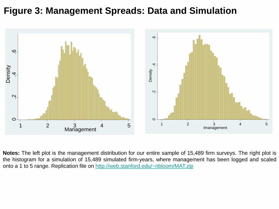
Figure 3: Management Spreads: Data and Simulation
Notes: The left plot is the management distribution for our entire sample of 15,489 firm surveys. The right plot is
the histogram for a simulation of 15,489 simulated firm-years, where management has been logged and scaled
onto a 1 to 5 range. Replication file on http://web.stanford.edu/~nbloom/MAT.zip
0.2
.4.6
De
nsity
1 2 3 4 5Management
0.2
.4.6
Density
1 2 3 4 5lmanagement

Figure 4: Management and Competition - Simulations
Elasticity of Demand
Notes: Results from using our estimated MAT model to simulate 5,000 firms per year in the steady state.
Plots log(management) in the simulation data normalized onto a 1 to 5 scale, and log(sales). Competitionis index by demand elasticity (ρ=5) in baseline. Dark Blue bar is unweighted mean across firms, Light Red
bar is weighted by firm size (employees). Replication file on http://web.stanford.edu/~nbloom/MAT.zip
Ma
nagem
ent
Score
1.5
22.5
33.5
44.5
3 4 5 6 7 8 10 12 15
Management Size-weighted management

Figure 5: Management and Firm Age - Simulations
Notes: Plots ln(management) scores weighted by age. Results from simulating 5,000 firms per year in the
steady state taking the last 10 years of data and defining age based on the number of observed years.
Management normalized to zero on the sample. Replication file on http://web.stanford.edu/~nbloom/MAT.zip
-.5
-.25
0.2
5.5
Man
ag
em
en
t m
ea
n
(norm
aliz
ed to z
ero
mean o
ver
the s
am
ple
-1-.
50
.51
Man
ag
em
en
t sp
read
(sta
nda
rd d
evia
tions)
1 2 3 4 5 6 7 8 9 10+
Firm Age
Management level
(sample normalized to 0)
Management spread

Figure 6: Management as Design
Notes: Results from the Management as Design model to simulate 5,000 firms in the steady state taking the last 10 years of data.
Plots log(management) in the simulation data normalized onto a 1 to 5 scale, and log(sales). See text for more details. Replication
file on http://web.stanford.edu/~nbloom/MAT.zip
Panel B: Management & Competition
1.5
22
.53
3.5
44
.5
3 4 5 6 7 8 10 12 15
management L weighted management
Elasticity of Demand
Ma
na
ge
ment
Panel D: Management & Performance
7.2
7.4
7.6
7.8
8
1 2 3 4 5
Management
Sa
les (
in lo
gs)
Panel C: Management & Age
-.2
5-.
15
-.0
5.0
5.1
5.2
5
Ma
na
ge
ment m
ea
n
-.7
5-.
5-.
25
0.2
5.5
.75
Ma
na
ge
ment std
1 2 3 4 5 6 7 8 9 10
Age
Management level
(sample normalized to 0)
Management spread
Panel A: The distribution of management
0.2
.4.6
1 2 3 4 5
Management
Den
sity

A) Management & Competition: Levels
Figure 7: Management and Competition
B) Management & Competition: Changes
Notes: Competition proxies are 1-Lerner = median firm profits/sales, Imports = imports/apparent consumption,
Imports China = imports from China/apparent consumption, all in industry by country cell. In “levels” panels control
for linear country & industry average. “Changes” are in deviations from time-specific country by industry dummies.

Figure 8. Management and Age - Data
Age bins1-5 6-10 11-15 16-20 21-25 26-30 31-35
-.0
20
.02
.04
.10
.12
.14
.16
35+
Notes: Data from 31,793 plants from the Management and Organizational Practices supplement to the 2010
Annual Survey of Manufacturing, run by the US Census. Mean management in deviation from the sample mean.
Management score from 0 (no modern practices adopted) to 1 (all 16 modern management practices adopted).
Management level
(sample normalized to 0)
Management spread
Man
ag
em
en
t m
ea
n
(norm
aliz
ed to z
ero
mean o
ver
the s
am
ple
Man
ag
em
en
t sp
read
(sta
nda
rd d
evia
tions)

-2.5 -2 -1.5 -1 -.5 0
United StatesJapanSwedenGermanyCanadaGreat BritainSingaporePolandFranceMexicoItalyAustraliaSpainVietnamChileTurkeyPortugalColombiaBrazilIrelandChinaNew ZealandIndiaKenyaGreeceArgentinaMyanmarNigeriaTanzaniaNicaraguaEthiopiaZambiaGhanaMozambique
Figure 9: Management and Reallocation by Country
Notes: Share-weighted management score differences relative to the US (in terms of management score standard deviations).
Length of bar shows total deficit, composed of the sum of the (i) the unweighted average management scores (black bar) and the
Olley-Pakes reallocation effect (red bar). Domestic firms only with management scores corrected for sampling selection bias.
Reallocation gap with the USUnweighted management score gap with the US

TABLE 1: CALIBRATED PARAMETERS FROM THE LITERATURE
Parameter Symbol value Rationale
Output-labor elasticity β 0.6 NIPA factor share.
Output-management elasticity γ 0.1 Bloom et al (2013)
Output-capital elasticity α 0.3 Implied from Constant Returns
Demand elasticity ρ 5 Bartelsman et al (2013)
AR(1) parameter on ln(TFP) ρA 0.885 Cooper and Haltiwanger(2006)
Standard deviation of ln(TFP) σA 0.453 Cooper and Haltiwanger(2006)*
Discount Factor β 1/1.1 Standard 10% interest rate
Capital depreciation rate δK 10% Standard accounting assumption
Capital resale loss ϕK 50% Ramey and Shapiro (2001)
Notes: The production function in MAT is 1
i i i i iY AK L M and the revenue function is ( ) a b c
i i i i iPY AK L M Fixed cost of production is normalized to 100 and
mean of ln(TFP) is normalized to 1.
* Assumes measurement error on measured TFP has the same variance as true TFP as estimated in Bloom et al (2013).

TABLE 2: ESTIMATED PARAMETERS USING SIMULATED METHOD OF MOMENTS
PANEL A: PARAMETER ESTIMATES FROM SMM
Parameter Symbol Value
Depreciation rate of management δM 0.119 (0.053)
Adjustment cost parameter for management γM 0.212 (0.062)
Adjustment cost parameter for capital γK 0.195 (0.047)
PANEL B: MOMENTS USED IN SMM ESTIMATES
Parameter Simulated Value Data Value
Standard deviation of 5 year management growth 0.554 0.564
Standard deviation of 5 year sales growth 0.929 0.948
Standard deviation of 5 year capital growth 0.870 0.875
Notes: These are the parameters we estimate using the model (see text). Calibrated parameters from Table 1. Estimation by SMM on the management- accounting panel dataset of
up to 4907 firms. Standard errors generated by moment block-bootstrap and moment derivatives taken around the estimated parameter values.

TABLE 3: PERFORMANCE REGRESSIONS
(1) (2) (3) (4) (5) (6) (7) (8) (9) (10)
Dependent
variable Ln
(Value
Added)
Ln
(Value
Added)
Ln
(Value
Added)
Ln
(Value
Added)
Ln
(Value
Added)
Ln
(Employees)
Profitability
(ROCE, %)
5 year
Sales
growth
Ln
(Tobin q)
Survival
(%)
Method OLS OLS OLS Fixed Olley OLS OLS OLS OLS OLS Effects Pakes
Management 0.316*** 0.148*** 0.139*** 0.028** 0.102*** 0.404*** 0.989*** 0.040*** 0.028* 0.006***
(z-score) (0.017) (0.015) (0.018) (0.013) (0.013) (0.014) (0.297) (0.013) (0.014) (0.002) Ln(Labor) 0.938*** 0.662*** 0.669*** 0.424*** 0.593***
(0.017) (0.026) (0.030) (0.058) (0.025)
Ln(Capital) 0.274*** 0.260*** 0.193*** 0.403***
(0.019) (0.022) (0.041) (0.009) General
controls No Yes Yes Yes Yes Yes Yes Yes Yes Yes
Observations 11,465 11,465 9,334 9,334 8,701 25,947 13,255 12,046 6,628 7,726
Notes: *** denotes significance at the 1% level, ** denotes 5% significance and * denotes 10% significance. All columns estimated by OLS (except column (5) which uses the
uses the Olley-Pakes estimator). Standard errors in parentheses under coefficients (clustered by firm except in column (5) which is bootstrapped with 150 replications). “Fixed
Effects” includes a full set of firm dummies. Columns (1) to (9) are run on the combined full management-accounting panel from 2004 to 2014 although number of observations
differs due to missing values. Column (10) is run on the 2011 cross-section using firms surveyed up until 2010, with this cut-off defined to provide 4 years to measure exit (firms
can take up to 4 years to show up as dead in accounting data). Columns (3) and (4) restrict to firms which were surveyed in at least two different years. Column (5) restricts to
firms with positive lagged investment data (the proxy variable in Olley-Pakes). “Management” is the firm’s normalized z-score of management (the z-score of the average z-
scores of the 18 management questions). “Profitability” is “Return on Capital Employed” (ROCE) and “5 year Sales growth” is the 5-year growth of sales defined as the
difference of current and 5-year lagged logged sales. All columns include a full set of country, time and industry dummies. “Survival” is the probability of not exiting by 2011,
conditional on being alive at some point in the 2004-2010 period (sample mean of exit is 2.4%). “Tobin’s Q” is the stock-market equity and book value of debt value of the firm
normalized by the book value of the firm, available for the publicly listed firms only. “General controls” comprises of firm age and the proportion of employees with college
degrees and firm age, plus a set of survey noise controls (interviewer dummies, the seniority and tenure of the manager who responded, the duration of the interview, the day of
week the interview was conducted and an indicator of the reliability of the information as coded by the interviewer). Column (10) omits noise controls because of collinearity due
to low number of exits.

TABLE 4: COMPETITION AND MANAGEMENT
(1) (2) (3) (4) (5) (6)
Dependent Variable: Management (z-scored)
(1-Lerner) 0.990*** 1.751***
(0.366) (0.443)
Import Penetration 0.398** 0.830**
(0.170) (0.327)
Import Penetration – from China only 2.090** 2.204*
(0.972) (1.137)
Observations 8,630 8,630 8,630 8,630 8,630 8,630
Size- weight the regressions? No Yes No Yes No Yes
Notes: ** indicates significance at 5% level and * at the 10%. The dependent variable in all columns is the z-score of the average z-scores of the 18 management
questions. OLS estimates with standard errors in parentheses below coefficients. Standard errors are clustered at the industry by country by period cell in all
columns. “Lerner” is the median gross price-cost margin across all firms (from the ORBIS population) in the firm’s three digit SIC industry by country by
period cell; “Import penetration” is the value of all imports divided by apparent consumption (total production + imports - exports) in the plant’s ISIC Rev3
industry by country by period cell. “Import penetration – from China only” is the value of all imports originating from China divided by apparent consumption
in the plant’s ISIC Rev3 industry by country by period cell. All columns include only firms located in OECD countries and include all data collected across
2004-2014 survey waves. Industry is defined at the 3 digit SIC level in columns (1)-(2), and at the ISIC Rev3 level in columns (3)-(6). All columns include
ln(firm employment) and ln(plant employment), plus a full set of country by industry dummies and general controls (firm age and the proportion of employees
with college degrees (from the survey), a set of survey noise controls which are interviewer dummies, the seniority and tenure of the manager who responded,
the duration of the interviews and an indicator of the reliability of the information as coded by the interviewer). Columns (1) and (2) include a variable measuring
the log of the number of firms used to build the Lerner index in the country-industry-period cell. Columns (3)-(6) include the variable measuring apparent
consumption in the country-industry-period cell (the denominator of the import penetration variable) in levels. Employment weights are defined with respect to
total employment in the industry (3 digit SIC) by country cell.
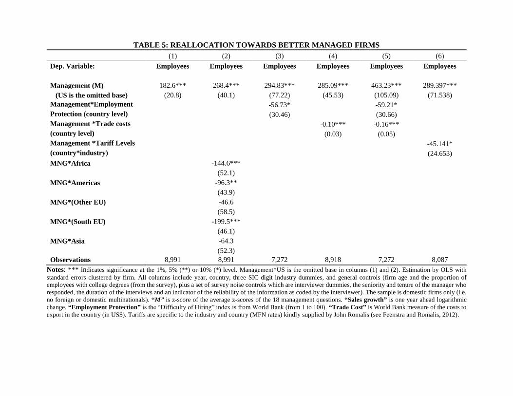
TABLE 5: REALLOCATION TOWARDS BETTER MANAGED FIRMS
(1) (2) (3) (4) (5) (6)
Dep. Variable: Employees Employees Employees Employees Employees Employees
Management (M) 182.6*** 268.4*** 294.83*** 285.09*** 463.23*** 289.397***
(US is the omitted base) (20.8) (40.1) (77.22) (45.53) (105.09) (71.538)
Management*Employment -56.73* -59.21*
Protection (country level) (30.46) (30.66)
Management *Trade costs -0.10*** -0.16***
(country level) (0.03) (0.05)
Management *Tariff Levels -45.141*
(country*industry) (24.653)
MNG*Africa -144.6***
(52.1)
MNG*Americas -96.3**
(43.9)
MNG*(Other EU) -46.6
(58.5)
MNG*(South EU) -199.5***
(46.1)
MNG*Asia -64.3
(52.3)
Observations 8,991 8,991 7,272 8,918 7,272 8,087
Notes: *** indicates significance at the 1%, 5% (**) or 10% (*) level. Management*US is the omitted base in columns (1) and (2). Estimation by OLS with
standard errors clustered by firm. All columns include year, country, three SIC digit industry dummies, and general controls (firm age and the proportion of
employees with college degrees (from the survey), plus a set of survey noise controls which are interviewer dummies, the seniority and tenure of the manager who
responded, the duration of the interviews and an indicator of the reliability of the information as coded by the interviewer). The sample is domestic firms only (i.e.
no foreign or domestic multinationals). “M” is z-score of the average z-scores of the 18 management questions. “Sales growth” is one year ahead logarithmic
change. “Employment Protection” is the “Difficulty of Hiring” index is from World Bank (from 1 to 100). “Trade Cost” is World Bank measure of the costs to
export in the country (in US$). Tariffs are specific to the industry and country (MFN rates) kindly supplied by John Romalis (see Feenstra and Romalis, 2012).

TABLE 6: MANAGEMENT BY DESIGN - STYLES DIFFER DEPENDING ON ENVIRONMENT
(1) (2) (3) (4) (5) (6) (7) (8) (9)
People
Management
Monitoring
& Targets
Relative
People
People
Management
Monitoring
&Targets
Relative
People
People
Management
Monitoring
&Targets
Relative
People
(P) (MT) (P-MT) (P) (MT) (P-MT) (P) (MT) (P-MT)
Panel A: Using US Four digit industry (NBER, NSF)
ln(K/L) 0.018 0.107*** -0.118*** -0.000 0.096*** -0.125***
(0.015) (0.016) (0.018) (0.014) (0.016) (0.019)
R&D Intensity 0.136** 0.041 0.114 0.031 -0.125* 0.201***
(0.064) (0.087) (0.089) (0.062) (0.072) (0.074)
ln(%degree) 0.139*** 0.123*** 0.011
(0.008) (0.007) (0.010)
Observations 13,681 13,681 13,681 13,681 13,681 13,681 13,681 13,681 13,681
Panel B: Two-Digit industry by county specific value (KLEMS, OECD)
ln(K/L) -0.044 0.039 -0.104** -0.062 0.038 -0.126***
(0.040) (0.032) (0.040) (0.040) (0.034) (0.037)
R&D Intensity 0.496 0.100 0.476* 0.584 -0.004 0.721**
(0.358) (0.260) (0.249) (0.413) (0.254) (0.306)
ln(%degree) 0.132*** 0.071*** 0.070***
(0.015) (0.012) (0.019)
Observations 4,855 4,855 4,855 4,855 4,855 4,855 4,855 4,855 4,855
Notes: *** denotes 1% significant, ** denotes 5% significance and * denotes 10% significance. All dependent variables are z-scores of average z-scores of the underlying
questions. “People management” is the index built using all management questions between 13 to 18 and “Monitoring and targets” are all the remaining questions. All
columns estimated by OLS with standard errors in parentheses under coefficients. All columns control for two-digit SIC industry dummies, country and year dummies, ln(firm
employment) and ln(plant employment), plus a full set of general controls (firm age and the proportion of employees with college degrees (from the survey), plus a set of survey
noise controls which are interviewer dummies, the seniority and tenure of the manager who responded, the duration of the interviews and an indicator of the reliability of the
information as coded by the interviewer). In Panel A the capital-labor ratio is taken from the NBER Bartelsman-Grey dataset and R&D intensity is business R&D divided by
employment from NSF. Both capital-labor and R&D intensity are at the four digit level for the US and used across all countries (so no country-specific variation). In Panel B
the capital-labor ratio is measured at the two digit by country level from the EU KLEMs dataset and R&D/Value added is from the OECD STAN/ANBERD. EU-KLEMS is
only available for a restricted set of countries (Australia, Germany, Italy, Japan, Sweden, UK and US) hence the smaller sample size. Standard errors are clustered at the four
digit level in Panel A and two-digit industry by country level in Panel B.

TABLE 7: DECOMPOSITION OF CROSS COUNTRY TFP AND MANAGEMENT
Weighted
Manage
ment
Un-
weighted
Manage
ment
OP
Covar-
iance
Mng.
Gap vs.
US
Reallocat
ion % of
Mng Gap
TFP
Index
relative
to US
% TFP
Gap due
to Man-
agement Country (1) (2) (3) (4) (5) (6) (7)
US 0.90 0.40 0.50 0 1
Japan 0.57 0.26 0.31 -0.33 56.64 0.71 9.71
Sweden 0.55 0.38 0.17 -0.35 93.39 0.92 43.49
Germany 0.36 0.18 0.19 -0.54 57.91 0.83 28.72
Canada 0.27 0.04 0.24 -0.63 41.92 0.88 48.64
UK 0.10 -0.11 0.21 -0.81 35.88 0.86 55.34
Singapore 0.07 -0.23 0.29 -0.84 24.69
Poland 0.04 -0.20 0.23 -0.86 30.69 0.80 39.26
France -0.01 -0.19 0.18 -0.91 35.29 0.84 52.52
Mexico -0.07 -0.30 0.23 -0.97 28.21 0.73 30.20
Australia -0.08 -0.18 0.10 -0.98 40.24 0.83 51.56
Italy -0.08 -0.18 0.10 -0.98 41.05 0.82 48.90
Spain -0.14 -0.50 0.36 -1.04 13.19 0.76 39.03
Vietnam -0.18 -0.50 0.32 -1.08 16.42
Chile -0.19 -0.48 0.29 -1.09 18.81 0.69 29.48
Turkey -0.20 -0.29 0.09 -1.10 36.92
Portugal -0.22 -0.43 0.20 -1.13 26.27 0.66 27.41
Colombia -0.23 -0.51 0.28 -1.13 19.28 0.52 17.21
Brazil -0.26 -0.51 0.25 -1.16 21.20 0.45 14.63
Ireland -0.29 -0.55 0.26 -1.19 20.33
China -0.31 -0.41 0.11 -1.21 32.49 0.41 13.44
NZ -0.33 -0.48 0.15 -1.23 28.44 0.79 51.00
India -0.34 -0.52 0.17 -1.25 26.07 0.48 17.20
Greece -0.40 -0.52 0.12 -1.30 29.09 0.25 37.48
Kenya -0.40 -0.55 0.14 -1.30 27.26 0.70 9.32
Argentina -0.41 -0.55 0.14 -1.31 27.74 0.68 34.84
Myanmar -0.45 -0.78 0.33 -1.35 12.58
Nigeria -0.61 -0.67 0.06 -1.51 28.85
Tanzania -0.67 -1.04 0.37 -1.57 7.96 0.26 11.74
Nicaragua -0.71 -0.89 0.19 -1.61 19.44
Ethiopia -0.85 -1.05 0.20 -1.75 17.09
Zambia -0.99 -1.05 0.06 -1.89 23.00 0.05 6.22
Ghana -1.03 -1.04 0.01 -1.94 25.49 0.14 9.69
Mzmbique -1.46 -1.60 0.13 -2.36 15.47 0.33 21.40
Average -1.14 29.68 0.62 29.94
Notes: Colum (1) is employment share weighted management z-score. Column (2) is the unweighted score and Column (3) is
the management-employment covariance. Column (4) is the weighted management score in column (1) relative to US . Column
(5) is the proportion of relative weighted management score in column (1) due to reallocation. The country’s TFP relative to
the US in column (6) is from Penn World Tables version 8.1. (Feenstra et al, 2015) available at
http://www.rug.nl/research/ggdc/data/pwt/v81/the_next_generation_of_the_penn_world_table.pdf. Column (7) is the fraction
of the TFP gap with the US in column (6) that is due to the weighted relative management score in column (1). We assume a
one standard deviation increase in the management score causes a 10% increase in TFP (using Table 3 and Bloom et al, 2013).
All scores are adjusted for nonrandom selection into the management survey (see text). Only domestic firms used in these
calculations (i.e. multinationals and their subsidiaries are dropped).

TABLE 8: ROBUSTNESS OF DECOMPOSITIONS
(1) (2) (3) (4) (5) (6)
Relative to US size-weighted
Management Score
Share of TFP gap with US accounted for
by size-weighted management
Countries Mean Correlation with
baseline Countries Mean
Correlation
with baseline
1. Baseline 33 -1.14 1 25 29.90 1
2. Drop pre-2006 data 33 -1.22 0.998 25 33.10 0.992
3. Drop panel firms after first year 33 -1.17 0.995 25 31.55 0.991
4. Just size in selection equation 33 -0.99 0.996 25 24.80 0.985
5. No Selection Correction 33 -0.86 0.984 25 19.97 0.873
6. Include multi-nationals 33 -1.02 0.854 25 24.43 0.888
7. Weighted inputs as size
measure 33 -0.98 0.990
25 34.48 0.960
8. Include firms outside 50,5000 13 -0.86 1 12 41.16 1
9. Include firms outside 50,5000 13 -1.08 0.925 12 49.98 0.968
Notes: This Table shows key statistics for alternative ways of dealing with potential sample selection concerns. The baseline in row 1 summarizes results in Table 7 where we
correct for country-specific sample selection (modelled from a first stage probit of whether an eligible firm responded as a function of ln(employment size), whether the firm
was publicly listed, and industry dummies). We then weight observations by the inverse of the probability of being in the sample. Row 2 drops all data before 2006. Row 3
drops all observations in the panel after the first year the firm is drawn in the sample. Row 4 uses only ln(employment) in the probit for sample selection. Row 5 uses the raw
data, i.e. does not correct for selection. Row 6 includes multinationals (the baseline results only use domestic firms) and includes a foreign multinational dummy in the selection
equation. Row 7 uses weighted inputs (capital and labor) as a size measure rather than just labor. Our sampling frame uses firms with between 50 and 5,000 employees. For a
sub-sample of countries we know the fraction of employment this covers differs across countries (see Appendix B for details) and can use this to impute management in the
“missing” part of the size distribution. We show the results of this in rows 8 and 9. Since this correction can only be done for the sub-sample of countries where we know the
full firm size distribution for manufacturing, row 8 shows what the baseline results look like for this sub-sample of countries and row 9 presents the corrected results. “Correlation
with baseline” is the correlation of the relevant (country level) variable with the baseline values in row 1. The correlation with size weighted management is in column (3) and
the correlation of the fraction of country TFP accounted for by management is in column (6).

TABLE 9: TFP SPREAD ACCOUNTED FOR BY MANAGEMENT PRACTICES
(1) (2) (3) (4)
Country Source Ln(TFP)
90-10
Management
90-10
Implied TFP
change
% TFP 90-10
accounted for by
Management
Australia OECD 1.93 2.68 0.27 14%
Chile OECD 2.97 2.77 0.28 9%
France OECD 1.42 2.72 0.27 19%
Italy OECD 1.57 2.56 0.26 16%
Japan OECD 1.15 2.48 0.25 22%
New Zealand OECD 1.93 2.58 0.26 13%
Sweden OECD 1.44 2.51 0.25 17%
UK Disney, Haskel and Heden (2000) 0.91 2.61 0.26 29%
US Syverson (2004) 0.90 2.55 0.26 28%
Average 19%
Notes: Column (1) reports the 90-10 spread in ln(TFP) in manufacturing. Column (2) reports the 90-10 spread in the standardized management score within each country. We
assume that a one standard deviation increase in the management score causes a 10% increase in TFP (using Table 3 and Bloom et al, 2013). Column (3) reports the implied
effect on ln(TFP) of an increase in the management score equivalent to the 90-10 management spread. Column (4) reports the fraction of the 90-10 ln(TFP) spread accounted
for by a 90-10 increase in the management score. The data on ln(TFP) for Australia, Chile, France, Italy, Japan, New Zealand and Sweden is drawn from OECD (2016). The
data for the UK is drawn from Disney, Haskel and Heden (2000). The data for the US is drawn from Syverson (2004). As noted in Section 1 these are all revenue based
measured of TFP (“TFPR”).

A APPENDIX: DATA
We overview the datasets in this Appendix. More information on an earlier version of the WMS
dataset can be found in Bloom, Sadun and Van Reenen (2012b) and Bloom and Van Reenen
(2007). More information on the management survey in general (including datasets, methods and
an online benchmarking tool) is available on http://worldmanagementsurvey.org/. Details on the
MOPS data is in Bloom et al (2017).
A.1 Firm-level Accounting Databases
Manufacturing firm sampling frame
For the WMS we focus on medium sized manufacturing firms, so to conduct our surveys we would
ideally draw a sampling frame from a business registry of firms. Unfortunately, the names of these
firms in administrative data from business registers (where it exists) are usually confidential. Three
exceptions were Chile, Colombia and Singapore. In Chile we worked directly with the government,
so it was possible to use the confidential business register data to phone firms - the Industrial
Annual Survey Sample of Firms (Encuesta Nacional Industrial Annual - ENIA), which covers all
manufacturing firms with more than 10 employees. We used a similar model in Colombia, working
with the Business Ministry and World Bank. In Singapore the Ministry of Trade and Industry ran
the survey (with our training) using their population business register.47
For other countries we use publicly available data sources.48 Our main sampling frame was based
on various accounting databases supplied by Bureau van Dijk (BVD), a private sector organization
that seeks to compile accounting information on companies from all over the world. BVD ORBIS
has names, industry, addresses, status (e.g. active or bankrupt), and accounting information such
as employment and sales. ORBIS is constructed from a range of sources, primarily the national
registries of companies (such as Companies House in the U.K.). The full sources for the sampling
frame are listed in column (3) of Table A2.49 In some countries we were concerned about incomplete
coverage by ORBIS so we supplemented it with other sources. We also used Dun & Bradstreet for
Australia and New Zealand. In India we use CMIE Firstsource 2005.50 Low income countries pose
47Unlike in Chile and Colombia, we were not able to obtain the characteristics of the non-responders in the samplingframe from the Singaporean government due to confidentiality reasons.
48There is usually a fee to be paid for access to the data compiled in an easy to use form, but the names andaddresses of the firms are given in this data (unlike administrative government data where names are not revealed)as they are in the public domain.
49The firm-level databases underlying ORBIS are sometimes packaged under different names in different regionsof the world by BVD (for a given country, the same firms are covered but sometimes with more fields of data). Forexample, in Europe the firm database is called AMADEUS (France, Germany, Greece, Great Britain, Italy, Ireland,Northern Ireland, Poland, Portugal, Spain, Sweden and Turkey); in North America it is called ICARUS (U.S. andCanada) and in parts of Asia it is called ORIANA (China, Japan). Other countries where we simply used ORBISinclude Argentina, Brazil, Mexico and Viet Nam. In Table A2 we simply refer to all of these as ORBIS as this is thesame overall list of firms.
50CMIE is constructed from the Registry of Companies in India. Icarus is constructed from the Dun & Bradstreet
31
APPENDICES INTENDED FOR ONLINE PUBLICATION ONLY

a particular challenge, as there is generally no well maintained business register to draw upon. We
used a larger variety of data sources to construct sampling frames for these countries complementing
ORBIS with country specific “enterprise maps” put together by researchers such as John Sutton
at the London School of Economics’ International Growth Centre (IGC), who worked with local
consultants. For full details on the African sampling frame, see Lemos and Scur (2015). Briefly,
in addition to ORBIS and the enterprise maps in Ethiopia (Sutton and Kellow, 2010), we also
used trade directories and the online yellow pages; in Ghana we supplemented Sutton and Kpentey
(2012) with the Ghana Free Zones Board and Business Ghana Directory; in Kenya we supplemented
ORBIS with the Kenya Association of Manufacturers; in Mozambique we supplemented Sutton,
Pimpao, Simione, Zhang and Zita (2014) with the Ministry of Commerce’s database and FACIM; in
Nigeria we supplemented ORBIS with VConnect; in Tanzania we supplemented Sutton and Olomi
(2012) with the Ministry of Trade database; in Zambia we supplemented Sutton and Langmead
(2013) with the Zambia Association of Manufacturers. In Myanmar we supplemented the PEDL
Enterprise Map with industry directories and lists of manufacturers provided by the Myanmar
Industry Association (see Tanaka, 2015) and in Nicaragua we used business directories and an
IADB database.
These databases all provide sufficient information on companies to conduct a stratified telephone
survey (company name, address, and a size indicator). They also typically have some accounting
information on employment, sales, and capital. We did not insist on having accounting information
to form the sampling frame, however.
Representativeness of the sampling frame
How representative are our sampling frames of the underlying population of manufacturing firms?
For most of the countries we have evidence that the data is reasonably comprehensive. For example,
when comparing aggregate employment in the ORBIS populations to those from census data, we
usually find a reasonably close match (e.g. Kalemli-Ozcan et al, 2015; Bloom, Draca and Van
Reenen, 2016).
In Bloom, Sadun and Van Reenen (2012b) we analyze this in more detail. For example, we compare
the number of employees for different size bands from our sampling frame with the figures for the
corresponding manufacturing populations obtained from national census data from each of the
countries where this is available. There are several reasons for a mismatch between Census data
and firm level accounts.51 Despite these potential differences, our sampling frame appears to cover
database, which is a private database of over 5 million US trading locations built up from credit records, businesstelephone directories and direct research. Oriana is constructed from Huaxia credit in China and Teikoku Databasein Japan, covering all public and all private firms with one of the following: 150 or more employees, 10 million US$of sales, or 20 million US$ of assets.
51First, even though we only use unconsolidated firm accounts, employment may include some jobs in overseasbranches. Second, the time of when employment is recorded in a census year will differ from that recorded infirm accounts. Third, the precise definition of “enterprise” in the census may not correspond to the “firm” incompany accounts. Fourth, we keep firms whose primary industry is manufacturing whereas census data includes only
32

near to the population of all firms for most countries. 52
Mismatch between the true population and our sampling frame could be a problem if our sampling
frame was non-randomly omitting firms - for example under-representing smaller firms - because it
would bias our cross-country comparisons. We tried several approaches to address this. First, in
almost all the regression tables we include country fixed effects to control for any differences across
countries in sample selection bias. Hence, our key results are identified by within country variation.
Second, we ran experiments where we dropped problematic countries (e.g. Portugal and Sweden)
from the analysis to show that the results are robust.
It is harder to make such comparisons between our sampling frame and the full population of firms
in some of the poorer countries as there is no reliable employment aggregate numbers to compare
to. The enterprise maps by Sutton and others that we draw our sampling frames from are probably
the most reliable sources. Given this, we should interpret some of the results from the African
countries with more caution than those of the other nations.
Medium sized manufacturing firms vs. all manufacturing firms
A further concern that is that even if our sampling frame is fully comprehensive, the proportion of
employment covered by medium sized firms differs systematically across countries. Using Census
sources on firm populations, Table A3 shows the employment distribution for the countries where
it is available. Firms employing between 50 and 5,000 workers account for about half of all man-
ufacturing workers in most countries, although the proportion was larger in some countries such
as Ireland (72%) and Poland (71%). The proportion employed by very large firms with over 5,000
workers varies more between nations. The patterns are broadly consistent with our MAT model.
In countries where competition is strong and reallocation easier, there is a larger fraction of jobs
in very large firms (e.g. 34.7% in the U.S.) and a small fraction in small firms with under 50
employees (e.g. 16.2% in the U.S.). Germany, also a high productivity and high management score
country, looks similar to the U.S. (34.9% in large firms vs. 16.5% in small firms). By contrast, in
countries like Italy and Greece, only 6.4% and 6.2% of employees respectively are in these large
firms compared to 45.1% and 41.3% in small firms. In Appendix B we provide some corrections to
our cross country decompositions to deal with the fact that we are missing management scores in
the very large firms in some countries (e.g. the U.S. and Germany) compared to other countries,
like those in southern Europe. As expected, these corrections strengthen our overall findings as
plants whose primary industry code is manufacturing. Fifth, there may be duplication of employment in accountingdatabases due to the treatment of consolidated accounts. Finally, reporting of employment is not mandatory for theaccounts of all firms in all countries. This was particularly a problem for Indian and Japanese firms, so for thesecountries we imputed the missing employment numbers based on a regression of sales on employment for firms wherewe had both variables.
52In two countries the coverage from accounting databases underestimates the aggregate: the Swedish data coversonly 62% of Census data and the Portuguese accounting database covers 72%. This is due to incomplete coverage inORBIS of these smaller nations.
33

the “corrected” relative average management scores for the U.S. and Germany rise compared to
southern Europe.
A caveat to Table A3 is that total employment in firms with over 5,000 workers is not disclosed
in all countries (because of concerns it would reveal individual firm’s identities). In the U.S. and
Japan we have the exact Census numbers from public use tables and in the U.K. we had access
to confidential Census micro-data to do this ourselves. In the other countries we used accounting
data from ORBIS and other sources to estimate employment for the very large firms. Since these
firms are so large, data is relatively plentiful as they are almost all publicly listed and so followed
closely by market analysts. 53
A.2 The World Management Survey
In every country the sampling frame for the management survey was all firms with a manufacturing
primary industry code and that employed between 50 and 5,000 workers54 on average over the most
recent three years of data prior to the survey.55Interviewers were each given a randomly selected list
of firms from the sampling frame. The size of this sampling frame by country is shown in column
(5) of Table A2 for the first year that we interviewed a firm. We have conducted the surveys over
multiple years as noted in column (6). The five major waves were in 2004, 2006, 2009/10, 2013
and 201456, although we had smaller scale surveys in some of the intervening years (e.g. China in
2007; Brazil, Canada and Ireland57 in 2008).
In the first survey in 2004 we covered 732 firms in France, Germany, the U.K. and the U.S.58 In
2006 we covered eight countries (China, Greece, India, Italy, Japan, Poland, Portugal and Sweden)
as well as the four core countries. In addition to the new countries and a refreshment sample
of the four 2004 countries we also re-contacted all firms from 2004 to form a short panel. In
53Corrections have to be made to estimate the number of domestic employees (which is the Census concept) if thisis not revealed directly by the firms. To do this we ran country specific regressions of the proportion of domestic overtotal global employment on a polynomial of total employment, industry dummies, and multinational status. Thenwe used this to impute the number of domestic workers for the firms who did not disclose domestic employment.
54In Japan and China we used all manufacturing firms with 150 to 5000 employees since Oriana only samplesfirms with over 150 employees.Note that the Oriana database does include firms with less than 150 employees if theymeet the sales or assets criteria, but we excluded this to avoid using a selected sample. We checked the results byconditioning on common size bands (above 150 in all countries) to ensure that the results were robust.
55In the U.S. only the most recent year of employment is provided. In India, employment is not reported for privatefirms, so for these companies we used forecast employment, predicted from their total assets (which are reported)using the coefficients from regressing ln(employees) on ln(assets) for public firms.
56Major waves were started in early summer, but sometimes stretched throughout the year. In 2009, the wavestretched through to the following February. We kept information on when the interview took place to control forany seasonal influences (a noise control).
57We split out Northern Ireland from the rest of the U.K. in Table A2 as we did an additional wave specifically ofNorthern Irish firms in 2008. Some of the Northern Irish firms were also surveyed in 2004, 2006 and 2010 as part ofthe general U.K. waves, but only a smaller number as the region is only a small part of the U.K..
58This sample was drawn from the BVD Amadeus dataset for Europe and the Compustat dataset for the U.S. Onlycompanies with accounting data were selected. So, for the U.K. and France, this sampling frame was very similarto the 2006 sampling frame. For Germany it is more heavily skewed towards publicly quoted firms since smallerprivately held firms report little balance sheet information. For the U.S. it comprised only publicly quoted firms. Asa robustness test we drop the firms that were resurveyed from 2004.
34

2009/10 we again resurveyed all firms interviewed 2006 including the original 2004 firms (if they
were still alive). For budgetary reasons we did not do a refreshment sample in this wave although
we did add New Zealand and Australia. In 2013 we mainly surveyed low income countries in Africa
(Ethiopia, Ghana, Mozambique, Nigeria, Tanzania and Zambia) and Latin America (Colombia and
Nicaragua) for the first time. But we also followed Argentina, Mexico and Brazil in the panel and
surveyed Spain and Turkey for the first time. In 2014 we included new countries (Kenya, Myanmar
and Vietnam) and performed refreshment samples of the U.S. and the main EU countries (France.
Germany, Greece, Italy, Portugal and the U.K.). This included attempting to re-survey all the
panel firms from the these EU countries and the U.S. that we had from earlier waves.
The Survey response rate
Column (4) of Table A2 shows the response rates by country. Of the firms we contacted 41% took
part in the survey, a high success rate given the voluntary nature of participation. Of the remaining
firms, 16% refused to be surveyed, while the remaining 43% were in the process of being scheduled
when the survey ended.
There are clear differences by country, with the response rate being lowest in Japan and highest in
Nigeria. Table A4 analyzes the probability of being interviewed.59 All columns condition on country
dummies, industry dummies and time dummies (for year of interview and year the accounting data
is taken from if different). The first column simply includes employment as a measure of size. The
size variable is significant suggesting that there was a tendency for large firms to respond more
frequently, although the coefficient is not large: a doubling of firm size is associated with only a
6% higher probability of response.
In column (2) of Table A4 we add in labor productivity and reassuringly find that firms with
higher revenues per employee are not significantly more likely to agree to be interviewed than others.
Column (3) includes the return on capital employed (ROCE) as an alternative performance measure
which is also insignificant. These are important results as they suggest we are not interviewing
particularly high or low performing firms. In columns (4), (5) and (6) we find that multinational
status, firm age, and capital are also all insignificant in the selection equations.
In summary, within a country, industry, and year, respondents were not significantly more pro-
ductive, profitable, or capital intensive than non responders. Respondents did tend to be slightly
larger, but were not more likely to be older or multinationals. Since all regressions include size,
country, industry, and time dummies, this potential source of bias is controlled for.
One concern, however, is that when we make cross country comparisons these selection effects
could create biases. Hence in our decomposition analysis we re-weight the data to allow for country
59The responders sample implicit in Table A4 is smaller than the total number of observations in Figure 1 for threereasons. First, we look only at the first time we contact a firm: this is because firms that appear in the panel arelikely to be better managed and more productive (since they survived longer). Second, we conduct the analysis atthe levels of the firm’s accounts and there may be multiple plants analyzed for the same firm in the same year. Third,we do not include Singapore because (as noted above) we do not have access to the non-responders.
35

specific sampling bias (see Appendix B and main text). Specifically, we ran probits of whether a
firm responded compared to others in the sampling frame where the right hand side variables are
employment, firm age, industry dummies and time dummies. We then calculated the probability
of sample response and used the inverse of the sampling probability as weights (winsorizing the top
and bottom percentiles).
Management - Accounting panel dataset
As described above, we have a panel element to the database. This is built by combining the
management survey waves with the accounting panel data, and then interpolating (but never ex-
trapolating) the management and accounting data to fill in the missing years. For example, if we
measure management practices every three years, we linearly interpolate the data in the interven-
ing years. This helps to increase the sample sizes for the five year difference moment since we do
not need to have exactly five years between survey waves (for example, without interpolating, if
we survey firms every three years we can never generate a five year difference). But, to confirm
our results are not dependent on interpolating, we checked we can successfully replicate Table 3
using non-interpolated data finding very similar results. We also have about 5% of firm-years with
multiple survey values, for which we take the average value of all continuous variables (including all
the overall management score) and the value from the chronologically first survey for the discrete
values (e.g. “plant county of location”, “ownership type” etc). 60 All regression standard errors
are clustered by firm so that the standard-errors are appropriately corrected for any potential serial
correlation in the errors induced by interpolation.
The sample size in the regressions depend on the number of non-missing variables (and specific re-
gressions will drop observations that are effectively redundant if they are absorbed by the controls).
In terms of sample size for the overall panel, we have 15,003 firm-year observations between 2004
and 2014 inclusive for the non-interpolated data and 25,953 observations for the interpolated data.
Only a sub-set of these observations have non-missing values on the elements for the production
functions. In addition, we condition on having a minimum number of 20 firm-year observations per
country in the regressions. This leaves us with 15,001 observations in the panel distributed over
18 countries –Argentina, Australia, Brazil, Chile, China, France, Germany, Greece, Ireland, Italy,
Japan, Mexico, Poland, Portugal, Spain, Sweden, the UK and US.
Firm-level variables
We have firm accounting data on sales, employment, capital, materials, profits, shareholder equity,
long-term debt, market values (for quoted firms), and payroll (the wage bill). Value added is
60For example, the coefficients (standard errors) on management for columns (1) to (4) from Table 3 with non-interpolated data are 0.274 (0.017), 0.142 (0.015), 0.123 (0.016) and 0.038 (0.014) respectively.
36

calculated as sales minus materials.61 We also collected information on whether the firm was
part of a multinational enterprise during the survey interview. We supplemented and verified this
information through BVD, web searches, and direct telephone inquiries to the firms. We also
collected specific questions on the multinational status of the firm (whether it owned plants abroad
and the country where the parent company is headquartered) to be able to distinguish domestic
multinationals from foreign multinationals.
We collected many variables through our survey, including information on plant and firm employ-
ment, the fraction of employees with a degree, organizational structure, how many competitors
managers thought they faced, etc.
Management practices were scored following the methodology of Bloom and Van Reenen (2007),
with practices grouped into four areas: operations (three practices), monitoring (five practices),
targets (five practices), and incentives (five practices). The shop-floor operations section focuses on
the introduction of lean manufacturing techniques, the documentation of processes improvements,
and the rationale behind introductions of improvements. The monitoring section focuses on the
tracking of performance of individuals, reviewing performance, and consequence management.62
The targets section examines the type of targets, the realism of the targets, the transparency of
targets, and the range and interconnection of targets. Finally, the incentives/people management
section includes promotion criteria, pay and bonuses, and fixing or firing bad performers, where
best practice is deemed the approach that gives strong rewards for those with both ability and
effort. Our management measure averages the z-scores of all 18 dimensions and then z-scores this
average again.
Industry level variables
Our basic industry code is the U.S. SIC (1997) three digit level - which is our common industry
definition in all countries except otherwise noted. We allocate each firm to its main three digit
sector (based on sales), covering 135 unique three-digit industries. There are at least ten sampled
firms in each industry for 97% of the sample.
The “Lerner index of competition” is constructed, as in Aghion et al (2005), as the cross-firm
median of (1-profit/sales) in a country-industry-time period cell. Profits are defined as EBIT
(earnings before interest and taxation) to include the costs of labor, materials, and capital, but
exclude any financing or tax costs. The source of accounting data used to build the index is ORBIS
population data for all countries (i.e. we do not condition on having any management data). We
first build the median Lerner index for every country-industry-year cell.63 We then average the
61Some firms report “costs of good sold” and not materials. In this case we estimate materials as costs of goodssold minus the wage bill. For observations which still had missing values for materials we assumed that the fractionof materials in sales was equal to the industry-year average.
62Since the operations and monitoring concepts overlap we often group them together as “monitoring”.63To reduce the influence of outliers, we drop observations below the 1th and above the 99th percentile of the
Lerner index.
37

yearly values over three three-years sub-periods: period 1, including years between 2004 and 2006;
period 2, including years between 2008 and 2010; and period 3, including 2012 and 2013 data (2013
being the last year for which we have full ORBIS extractions). This timing roughly corresponds
to pre-crisis, crisis and post-crisis periods. These time varying measures of the Lerner index are
matched to the management interviews according to the year in which these were conducted (2004-
2006 for period 1; 2008-2010 for period 2; and 2012-2014 for period 3).
The variable “Import penetration” is built using data drawn from the World Input-Output Database
(WIOD). Import penetration is built as the share of imports over apparent consumption (total
production minus exports plus imports). This measure is built at the country by industry by year
level and then, similarly to the Lerner index, averaged across sub-periods. Since the last available
year for the WIOD is 2011, we use only two sub-periods, 2004-2006 (matched with management data
collected between 2004-2006) and 2008-2010 (matched with management data collected between
2008-2014). The industry classification is ISIC, Rev 3.
The variable “Import penetration from China” is built exactly as the “Import Penetration” variable,
except that it includes only imports originating from China in the numerator.
Tariff data was kindly supplied by Feenstra and Romalis (2015) and is at the country by industry
(SITC, Rev 4) by year (2000-2006) level. Since we have limited time series variation, we collapse
the data to the country by industry level.
Country level variables
We take country level measures of GDP per capita and TFP from the latest Penn World Tables
(Timmer et al, 2015). The OECD “Difficulty of Hiring” index (ranging from 1 to 100) is the variable
EPRC V2 (available for all years in the interval 1998-2013), and is drawn from their indicators of
employment protection. These are synthetic indicators of the strictness of regulation on dismissals
and the use of temporary contracts, compiled from 21 items covering three different aspects of
employment protection regulations as they were in force on January 1st of each year. We also
employ the variable “Cost to export (US$ per container)” drawn from the World Bank “Doing
Business” dataset (2015) which reflects the cost of obtaining export licenses and average container
costs.
A.3 Management and Organizational Practices Survey (MOPS)
MOPS was jointly funded by the U.S. Census Bureau and the National Science Foundation as
a supplement to the Annual Survey of Manufactures (ASM). The original design was based on
the same concepts as the WMS and was adapted to the U.S. through several months of devel-
opment and cognitive testing by the Census Bureau. It was sent by mail and electronically to
the ASM respondent for each establishment, which was typically the accounting, establishment, or
human-resource manager. Most respondents (58.4%) completed the survey electronically, with the
38

remainder completing the survey by paper (41.6%). Non-respondents were given up to three follow-
up telephone calls if no response had been received within three months. The survey comprised 36
multiple choice questions about the establishment, taking about 20 to 30 minutes to complete. The
survey included 16 questions on management practices covering (like WMS) monitoring, targets
and incentives.
The monitoring section asked firms about their collection and use of information to monitor and
improve the production process. For example, firms were asked how frequently performance indi-
cators were tracked at the establishment, with options ranging from “never” to “hourly or more
frequently”. The targets section asked about the design, integration, and realism of production
targets. For example, firms were asked what the time-frame of production targets was, ranging
from “no production targets” to “combination of short-term and long-term production targets”.
Finally, the incentives section asked about non-managerial and managerial bonus, promotion and
reassignment/dismissal practices. For example, it asked how managers were promoted at the es-
tablishment, with answers ranging from “mainly on factors other than performance and ability, for
example tenure or family connections” to “solely on performance and ability”. The full question-
naire is available on http://bhs.econ.census.gov/bhs/mops/form.html.
In our analysis, we aggregate the results from these 16 check box questions into a single measure of
structured management. The structured management score is the unweighted average of the score
for each of the 16 questions, where each question is first normalized to be on a 0-1 scale. Thus
the summary measure is scaled from 0 to 1, with 0 representing an establishment that selected the
bottom category (little structure around performance monitoring, targets, and incentives) on all
16 management dimensions, and a 1 representing an establishment that selected the top category
(an explicit focus on performance monitoring, detailed targets, and strong performance incentives)
on all 16 dimensions. As with WMS, we asked a range of questions about the characteristics of the
workers, firms, and collected variables that we used to approximate for interview noise (interviewee,
interview and interviewer characteristics).
The MOPS survey was sent to all ASM establishments in the ASM mail-out sample. 37,177
filled surveys were received, implying a response rate of 78%, which is extremely high for firm
surveys.We further restricted the sample for establishments with at least 11 non-missing responses
to management questions and also have positive value added, positive employment and positive
imputed capital in the ASM. In addition to our management data we use establishment level data
on sales, value-added and labor inputs from the ASM. The mean establishment size is 167 employees
and the median is 80. The average establishment in our sample has been in operation for 22 years,
44% of managers and 9% of non-managers have college degrees, 13% of their workers are in unions,
42% export and 69% are part of larger multi-plant firms.
More details on the MOPs survey are contained in Bloom et al (2017).
39

B APPENDIX: FURTHER RESULTS
B.1 Alternative Methods of estimating the productivity equation
We considered a large number of alternative approaches to estimating the productivity regression,
some of which are contained in Table A5. First, in column (1) we consider a standard “Solow Resid-
ual” approach deducting ln(labor) and ln(capital) from ln(value added) using three-digit industry-
specific shares in nominal value added as weights for the factor inputs. A regression of this TFP
measure on management has a highly significant coefficient of 0.080.
The next three columns embody alternative popular econometric approaches to estimating produc-
tion functions Column (2) reports the Blundell and Bond (2000) system GMM approach for our
standard specification of column (2) in Table 3. Here, we treat all factor inputs as endogenous
and use lags as instruments (lagged levels in the difference equations and lagged differences in the
levels equation). The unrestricted specification includes a lagged dependent variable and lags of the
factor inputs (see Appendix C.1 below). The common factor (COMFAC) restrictions are imposed
by minimum distance and the structural coefficients presented in the table. The management co-
efficient is about 0.05.64Column (3) presents the Levinsohn and Petrin (2003) approach where we
use materials (rather than investment) as the proxy variable. Column (4) reports the Olley-Pakes
approach (as in column (5) of Table 3) except we use the Ackerberg, Caves and Frazer (2015)
correction. The range of the estimates of the management coefficient is significant and positive
throughout and in magnitude lies within the range of those in Table 3 with Blundell-Bond giving
the lowest estimates and Levinsohn-Petrin the highest.
In columns (5) through (10) of Table A5 we repeat the specifications in Table 3 except we implement
output based production functions instead of value added based version. Hence we also include
material inputs on the right hand side. Column (5) has the whole sample, column (6) conditions on
firms surveyed in at least two years, column (7) presents firm fixed effects and column (8) has the
Blundell-Bond results. As expected, the factor input coefficients tend to be smaller in magnitude
than their counterparts for the value added function, but all remain significant.
The last four columns again present results with sales as the dependent variable, but drop materials
from the right hand side. Although the magnitude of the coefficient on management varies with
the different estimation approaches, it is positive and significant in every specification. We also
considered a wide variety of other approaches to production function estimation, for example using
the wage bill instead of employment as a measure of labor services (as in Hsieh and Klenow, 2009).
The significance of management remained in all of these experiments.
64Note that this is the econometric specification closest to the theoretical model–lags are legitimate instrumentsunder the quadratic adjustment model we have assumed (Bond and Soderbom, 2005). We generalize the theorymodel slightly as we (implicitly) also allow labor to also have adjustment costs alongside capital and management.Interestingly, the sum of the coefficients on the factor inputs is 0.8, lower than the OLS levels and Olley-Pakesestimates in Table 3. This is consistent with the calibrated parameter values from Table 1 which has constant returnsin production but CES monopolistic competition with a demand elasticity of 5 which means the coefficients in therevenue function should be 20% smaller than the output elasticities in the production function.
40
B.2 The contribution of management to cross country TFP gaps: Robustness
In Section 5 we decomposed share-weighted management into reallocation and unweighted average
components and use this to estimate the contribution to cross country TFP. In doing that, we
made a variety of assumptions that we now relax to see if they materially alter our results. Recall
that (i) the sample we used in the analysis is a sub-sample of that underlying Figure 1 as we drop
multinationals because it is unclear what the appropriate measure of size is for such firms (we also
show robustness to including multinationals); and (ii) we weight the management data according to
a firm’s country-specific employment share and adjust for non-random selection through sampling
weights.
B.2.1 Differential response rates to the survey
There are several potential sources of sample selection, the most obvious one being that the firms
who responded from the sampling frame were non-random in some dimension. Appendix A exam-
ined the overall evidence on sampling bias and argued that these were relatively small. Nevertheless,
the baseline results in Table 7 control for this by calculating (country-specific) weights for the sam-
ple response probabilities. We do this by running country-specific probit models where the control
variables are ln(employment size), firm age, a dummy for whether the firm was publicly listed and
industry dummies. We chose these controls because they are available for responders and non-
responders, and there was some evidence from Appendix A that larger firms were more likely to
respond. We then calculated the weights as the inverse of the probability of response.
We experimented with an alternative first stage probit to look into sample response bias, based
on just using employment rather than the larger set of controls. The results are summarized in
Table 8. Row 1 presents a summary of the baseline results that we use in Table 7. Row 2 shows
what happens when we drop pre-2006 data. This is motivated by the fact that 2004 was our first
(and smallest) survey wave. The fraction of the TFP gap accounted for by management rises to
33% (from 30%). We also show in column (6) that the correlation of this fraction explained with
the baseline in row 1 is very high (0.992) and the correlation of the gaps in management with the
baseline of Row 1 are also very high (0.998 in column (3)). Row 3 drops all observations which are
in the panel part of the dataset except the first year. The motivation for doing this is that firms who
have been in the panel for one year are more likely to respond in subsequent years than a randomly
chosen firm. Since we attempt to re-sample panel firms in subsequent years this could potentially
generate a bias. In the baseline results of Row 1 we down-weight these firms appropriately using
estimate from the probits. Row 3 shows that our results are robust to just dropping them from
the sample (32% of TFP accounted for). We also looked at the sensitivity of the first stage probit
to the controls by dropping all covariates except size (row 4) and not using any sample weights
(row 5). Not using any selection correction generates the smallest fraction of the TFP explained in
Table 8 (20%).
41

In Table 7, we dropped multinationals because of the difficulty of measuring group size appropriately
for such companies. To check the robustness of these results, we included them in row 6, but also
included multinational status into the selection equation used to calculate the sample response rate
weights (multinationals were slightly more likely to participate in the survey). We account for a
bit less of the average TFP gap (24% compared to 30% in the baseline) and the cross country
correlation remains reasonably high (0.89).
We have focused on employment as our key measure of size as it is simple, a volume indicator which
is straightforward to measure across countries. An alternative way to measure size is to look at a
measure of weighted inputs, so we follow Bartelsman et al (2013) and construct a measure using
capital stock information from Orbis where our composite input measure was exp[0.7*ln(labor) +
0.3*ln(capital)]. The results are in row 7 of Table 8 and are again are similar to the baseline,
although with slightly more of TFP accounted for by management (34.5%).
B.2.2 Sampling biases associated with dropping very small and very large firms
Our management surveys focus on medium sized firms defined as those with over 50 and under
5000 employees. This was in order to compare firms of a broadly similar size. However, it could
potentially cause bias in our comparisons of management levels across countries as the size distri-
bution is different across nations (e.g. Garicano, Lelarge and Van Reenen, 2013, and Table A3).
Obviously we do not know the exact distribution of management scores in these very large and
very small firms, but we can estimate with additional assumptions what the potential biases could
be.
From the census manufacturing population databases of firm demographics, in most countries we
know the number of firms above and below 50 employees, and the total number of workers employed
across firms of different sizes (see Table A3). We need to then make an assumption about the
relationship between firm size and management for the very large and very small firms, which we
extrapolate off the size-management relationship over the part of the distribution that we observe
(50 to 5,000 employees). We checked that the extrapolated size-management relationship holds for
firms below 50 and above 5,000 using the MOPs dataset which asks management questions to firms
from all parts of the U.S. size distribution.65
We then use this information to estimate the weighted average management score across the entire
distribution. Our preferred method exploits the fact that the firm size distribution in each country
follows a power law (Axtell, 2001). Using results from this literature we can approximate the
employment weighted mean management score in the sub-population under 50 workers and the
sub-population with over 5,000 workers.66 We then use the information in Table A3 to calculate
65The coefficient on ln(employment size) in the management regression is 0.25. We considered imposing a commonconstant on each country (-1.46) or adjusting this to be consistent with the country-mean management score in the50 to 5,000 range. Both methods lead to similar results.
66First, we consider the approximation in Johnson et al (1994) showing that the number of employees in each size
42

the mean management score across the entire size distribution. Results of this exercise are in rows
8 and 9 of Table 8. We first reproduce the baseline results on the smaller sample of countries in
row 8 of Table 8. In this sub-sample of 14 countries (13 differences as the U.S. is the base) we
account for a higher fraction of TFP (41%) since these are OECD countries. We then implement
the size correction. The correlation between our baseline management scores and the new “size
corrected” management scores is very high (0.925), as is the correlation of the fraction of TFP
explained (0.968). If anything, we account for an even higher fraction of the TFP gap (just under
50%) when making this correction.
B.2.3 Manufacturing TFP vs. Whole Economy TFP
The management scores are derived from manufacturing firms, but the decompositions in Table
7 use economy wide TFP. This is purely due to data restrictions - there are few countries in
the world for which it is possible to construct reliable measures of manufacturing TFP that are
comparable across countries. Our assumption is that countries with high economy wide TFP also
have high manufacturing TFP. To test whether this might bias our results, we draw on estimates of
manufacturing specific TFP levels (Citino, Haskel and Van Reenen, 2016). This is based primarily
on the KLEMs data and constructs TFP in the same way as the Penn World Tables, correcting for
capital services and skills. There are only seven countries that overlap between the two exercises
where data is sufficiently rich: Australia, Germany, Italy, Spain, Sweden, the U.K. and U.S. The
correlation of manufacturing TFP (relative to the U.S.) for these countries with economy TFP is
reassuringly high: 0.938. The average proportion of the TFP gap accounted for by management is
35%, similar to the overall mean (but smaller than the proportion for just the seven countries in
the baseline which is 43%).67
C CALIBRATION AND SIMULATION
C.1 Calibration Values
The calibration values in Table 1 are conventional, but the presence of management in the pro-
duction function generates some additional considerations. Conventional measures of the auto-
correlation coefficient on TFPR (ρA) assume that we have measured all factor inputs, but since
“bin” is equal when the bins are logarithmically sized if firm size is distributed according to Zipf’s Law (which isapproximately true in the data). We predict management in each bin and then employment weight the bin to obtainmean management for the below 50 and above 5,000 firms. We also considered the continuous version of the powerlaw which lead to similar results.
67We performed a similar exercise for the market sector (i.e. dropping health, education and public administration).For this sample we do not have Australia, but we do can add France. Again the correlation of TFP between thissector (market sector) and total economy is high at 0.844. We could account for 43.6% of the cross country TFPgaps, very similar to the fraction for these seven countries in Table 7 (44.7%).
43
managerial capital is a missing variable, it will implicitly show up in estimated TFPR. For ex-
ample, consider the value added production function in Section 2, (PY )i = AiKai L
biM
ci . TFPR
will be lnAi = ln(PY )i − alnKi − blnLi − clnMi. A standard way to measure TFP is replace the
parameters with cost shares. This has the problem that management shows up in the residual so
we actually have lnAi + clnMi. This implies that we probably overestimate the auto-correlation
of “true TFPR” by using existing measures as M and A will co-vary together. We can assess
this by examining how our estimates of TFPR in the data compare with those from conventional
measures. We find that the estimated coefficient is, in fact, not much less than the calibrated value
from Cooper and Haltiwanger (2006) of 0.885. For example, using the productivity equation of
column (2) in Table 3, we can calculate the (net-of-management) TFPR residual and then estimate
an AR(1) regression which generates ρA = 0.867 (standard error = 0.009; observations=7,463).
This is close to the 0.871 if we do not control for management in our data. The similarity reflects
the fact that management capital is a relatively small share of total value added.
An alternative approach is to use the implied values in the dynamic version of the revenue function.
Under the assumptions in our model we can write ln(PY )it = ρAln(PY )it + alnKit − aρAlnKit +
blnLit−baρAlnLit+clnMit−cρAlnMit+eit where eit = lnA0 +ρAεit which is serially uncorrelated.
This is the same specification as Cooper and Haltiwanger (2006) and Blundell and Bond (2000) and,
like them, we estimate the equation by system GMM and impose the common factor restrictions
(COMFAC) to recover the structural parameters (see Table A5 column (2)). Our estimate of (ρA)
is 0.854 (standard error = 0.013) which is again, very close to the calibrated value used in Table
1.68
As noted in the text we use labor’s factor share in GDP to guide the calibration of the output
elasticities. It seems reasonable to assume that the cost of managerial capital shows up as payments
to labor (e.g. executive time and consultancy wages). Recall that our structural model implies that
the total labor share in GDP is (β+γ)(ρ−1)/ρ. From the US NIPA this is currently about 56% (see
Autor et al, 2017, Table 1). Hence, given the other calibrated assumptions on the demand elasticity
(Bartelsman et al, 2013;ρ = 5) and output elasticity of management (Bloom et al, 2013;γ = 0.1 ) we
can then derive the output elasticity of labor as β = −γ+0.56ρ/(ρ−1) = −0.1+(0.56∗5)/(5−1) =
0.60. Consequently, from our assumption of constant returns to scale in production we also have
the output-elasticity of non-managerial capital as α = 1− β − γ = 1− 0.6− 0.1 = 0.1.
C.2 Details of Simulated Method of Moments (SMM) Approach
SMM starts by selecting an arbitrary starting value of the parameter vector to be estimated (θ).
The dynamic program is then solved and the policy functions are generated. These policy functions
are used to create a simulated data panel of size (µN, T ), where µ is a strictly positive integer, N
68A similar exercise for the standard deviation of TFPR (σA) generates a value of 0.62 which is higher than thecalibrated value of 0.453 in Cooper and Haltiwanger (2006). In our view, these higher order moments are betterestimated from near population Census data, so we prefer to use these external measures than our more specificsample.
44

is the number of firms in the actual data, and T is the time dimension of the actual data. The
simulated moments ΨS(θ) are calculated on the simulated data panel, along with an associated
criterion function Γ(θ), where Γ(θ) = [ΨA−ΨS(θ)]′W [ΨA−ΨS(θ)], which is a weighted distance69
between the simulated moments ΨS(θ) and the actual moments ΨA.
θ = arg minθ∈Θ
[ΨA −ΨS(θ)]′W [ΨA −ΨS(θ)] (12)
A second parameter value is then drawn by taking a random jump from the first value, and the third
parameter value onwards is drawn by taking a random jump away from the best prior guess (the
parameter value that has delivered the lowest criterion function up to that point). This way, the
parameter estimate θ derived by randomly searching over the parameter space to find the parameter
vector, which minimizes the criterion function. This simulated annealing random jumping approach
is used because of the potential for discontinuities in the model and the discretization of the state
space (so a gradient minimization approach may simply find a local rather than a global minimum).
Finally, different initial values of θ are selected to ensure the solution converges to the global
minimum.
D EXECUTIVE PAY AND MANAGEMENT
We discussed the relationship between payments to senior management and management practices
in the main text in sub-section 4.4. This Appendix gives more details on the data collection and
analysis.
Compensation data was collected for executives in publicly listed firms in four countries: the US,
UK, India, and China. There is an overall measure of CEO Compensation as well as a disaggre-
gation into salary, bonus and equity. In some cases, an executive’s total compensation exceeds
the sum of the components–e.g. in cases where the executive received separate perquisites such
as retirement benefits. Stock options are valued using the Black-Scholes formula. Data on equity
compensation is not available for executives in Indian firms, and data on bonus compensation are
not available for executives in Chinese firms. Due to these data limitations for Indian and Chinese
firms, regressions that use the total compensation measure include only executives from firms the
US and UK. Executive Compensation in the US is from S&P Capital IQ’s ExecuComp and the UK
the data is taken from BoardEx. For India we use Prowess, and for China we use the China Stock
Market & Accounting Research database. For comparability across time and across countries, all
compensation values are converted to 2006 PPP-adjusted dollars.
We focus on the relationship between a firm’s managerial quality and the compensation of its top
executive. In American firms, the top executive is typically the Chief Executive Officer. In other
69The efficient choice for W is the inverse of the variance-covariance matrix of [ΨA−ΨS(θ)], which Lee and Ingram(1991) show under the null can be calculated from the variance-covariance of the empirical moments.
45

countries, the exact title of the top executive varies. We use “CEO” to refer to each firm’s top
executive. After merging these data with the WMS we have a sample of 532 firms: 242 in the
US, 107 in the UK, 132 in India, and 51 in China. Unless otherwise specified, we use each firm’s
management score and compensation data from the year in which the management survey was
conducted for the firm.
Table A6 shows the results of regressing ln(CEO salary) on our management score and country
dummies in all four countries. There a positive and significant association between higher man-
agement scores and higher CEO pay. Column (2) controls for a number of other variables such as
firm size, age and skills. This reduced the coefficient on management from 0.309 to 0.189, but it
remains significant. The final two columns repeat these specifications but use a measure of total
compensation that includes stock options, long-term incentive plans and bonuses. This data is only
available in the UK and US. Despite the loss of sample, the management remains positively and
significantly associated with CEO compensation with a similar pattern of coefficients to the earlier
columns
The Social Security Data comes directly from Song et al (2017), which in turn is obtained from
the Master Earnings File in the Social Security Earnings, which contains the labor (W2) earnings
(uncapped) of all employees in the US from 1978 to 2013. The values provided in text are for 2013
for all firms defined as a single Employee Identification Number in a given year.
References
[1] Autor, David, David Dorn, Larry Katz, Christina Patterson and John Van Reenen (2017)“The Rise of Superstar firms and the fall of the Labor Share” NBER Working Paper 23396
[2] Axtell, Robert. 2001. “Zipf Distribution of U.S. Firm Sizes.” Science, 293(5536): 1818-1820.
[3] Bloom, Nicholas, Raffaella Sadun, and John Van Reenen. 2012b. “The Organization of FirmsAcross Countries.” Quarterly Journal of Economics 127(4): 1663-1705.
[4] Bond, Stephen and Mans Soderbom. 2005. “Adjustment costs and the identification of Cobb-Douglas production functions” IFS Mimeo
[5] Citino, Luca, Jonathan Haskel and John Van Reenen. 2016. “Accounting for the U.K. Pro-ductivity Gap.” London School of Economics mimeo.
[6] Garicano, Luis, Claire Lelarge and John Van Reenen. 2016. “Firm Size Distortions and theProductivity Distribution: Evidence from France” American Economic Review 106(11): 3439-79
[7] Johnson, Norman, Adrienne Kemp and Samuel Kotz. 1993. Continuous Univariate Distribu-tions. New York, N.Y.: John Wiley & Sons.
46

[8] Kalemli-Ozcan, Sebnem, Bent Sorensen, Carolina Villegas-Sanchez, Vadym Volosovych, Sev-can Yesiltas. 2015. “How to Construct Nationally Representative Firm level data from theORBIS Global Database” NBER Working Paper 21558.
[9] Lee, Bong-Soo and Beth Ingram. 1991. “Simulation Estimation of time series models” Journalof Econometrics 47(2-3) 197-205
[10] Lemos, Renata and Daniela Scur. 2015. “A snapshot of mid-sized firms in Africa, Asiaand Latin America.” Oxford University mimeo, http://worldmanagementsurvey.org/wp-content/images/2010/08/lemos scur snapshot dec20151.pdf.
[11] Levinsohn, James and Amil Petrin. 2003. “Estimating Production functions using inputs tocontrol for unobservables” Review of Economic Studies 70(2) 317-341
[12] Sutton, John and Bennet Kpentey. 2012. Enterprise Map of Kenya. London: IGC.
[13] Sutton, John, Jeque Pimpao, Felix Simione, Qi Zhang and Samuel Zita. 2014. Enterprise Mapof Ghana. London: IGC.
[14] Sutton, John and Donath Olomi. 2012. Enterprise Map of Mozambique. London: IGC
[15] Sutton, John and Gillian Langmead. 2013. Enterprise Map of Zambia., London: IGC, London:IGC.
[16] Tanaka, Mari. 2015. “Exporting Sweatshops: Evidence from Myanmar.” Stanford Universitymimeo.
47

2 2.2 2.4 2.6 2.8 3 3.2 3.4
United States
Germany
Sweden
Canada
United Kingdom
France
Italy
Australia
Singapore
Mexico
Poland
Portugal
China
Chile
Greece
Spain
Brazil
Argentina
India
Notes: Unweighted means of management scores by companies belonging to foreign multinationals vs. domestic firms (including
domestic multinationals). Countries with 60 or more + foreign multinationals only (sample of 13,544 interviews).
Foreign multinationals
Domestic firms
Figure A1: Foreign multinationals vs. domestic firms
Management Score

910
11
12
13
Lo
g S
ale
s
1 2 3 4 5Management
Figure A2: Firm Size is increasing in management
Notes: This plots the lowess predicted values of log(sales) against management (bandwidth=0.5).
Sales is log(sales) in US$. N=13,854
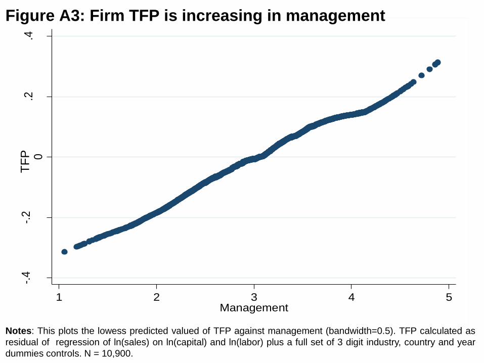
-.4
-.2
0.2
.4
low
ess
: R
esi
dua
ls
1 2 3 4 5Management
Figure A3: Firm TFP is increasing in management
Notes: This plots the lowess predicted valued of TFP against management (bandwidth=0.5). TFP calculated as
residual of regression of ln(sales) on ln(capital) and ln(labor) plus a full set of 3 digit industry, country and year
dummies controls. N = 10,900.
TF
P

Figure A4: Firms with higher management scores have higher
CEO compensation
Notes: These are 413 publicly firms in the UK and US. The line is the lowess predicted valued of the log of total
CEO compensation including salaries, bonuses and equity (in deviations from country averages) and the
management score.

0 20 40 60 80 100
SwedenCanadaGreat BritainFranceGermanyAustraliaItalyPolandNew ZealandSpainMexicoJapanGreeceChileArgentinaPortugalColombiaIndiaBrazilChinaMozambiqueTanzaniaKenyaGhanaZambia
Figure A5: TFP Gap accounted for by management
Notes: TFP gaps from Penn World Tables; fraction accounted for by management uses the weighted average
management scores and an assumed 10% impact of management on TFP. See Table 7 for details of
calculations. Vertical line indicates the mean effect (30%).
% of TFP gap accounted for by managementTFP level (Relative to US)

TABLE A1: MANAGEMENT PRACTICES QUESTIONNAIRE
Any score from 1 to 5 can be given, but the scoring guide and examples are only provided for scores of 1, 3 and 5. The survey also includes a set of Questions that
are asked to score each dimension, which are included in Bloom and Van Reenen (2007).
(1) Modern manufacturing, introduction
Score 1 Score 3 Score 5
Scoring grid: Other than Just-In-Time (JIT) delivery from
suppliers few modern manufacturing
techniques have been introduced, (or have
been introduced in an ad-hoc manner)
Some aspects of modern manufacturing
techniques have been introduced, through
informal/isolated change programs
All major aspects of modern manufacturing have been
introduced (Just-In-Time, autonomation, flexible
manpower, support systems, attitudes and behaviour) in
a formal way
(2) Modern manufacturing, rationale
Score 1 Score 3 Score 5
Scoring grid: Modern manufacturing techniques were
introduced because others were using them.
Modern manufacturing techniques were
introduced to reduce costs
Modern manufacturing techniques were introduced to
enable us to meet our business objectives (including
costs)
(3) Process problem documentation Score 1 Score 3 Score 5
Scoring grid: No, process improvements are made when
problems occur.
Improvements are made in one week
workshops involving all staff, to improve
performance in their area of the plant
Exposing problems in a structured way is integral to
individuals’ responsibilities and resolution occurs as a
part of normal business processes rather than by
extraordinary effort/teams
(4) Performance tracking
Score 1 Score 3 Score 5
Scoring grid: Measures tracked do not indicate directly if
overall business objectives are being met.
Tracking is an ad-hoc process (certain
processes aren’t tracked at all)
Most key performance indicators are tracked
formally. Tracking is overseen by senior
management.
Performance is continuously tracked and communicated,
both formally and informally, to all staff using a range of
visual management tools.

(5) Performance review
Score 1 Score 3 Score 5
Scoring grid: Performance is reviewed infrequently or in
an un-meaningful way, e.g. only success or
failure is noted.
Performance is reviewed periodically with
successes and failures identified. Results are
communicated to senior management. No
clear follow-up plan is adopted.
Performance is continually reviewed, based on indicators
tracked. All aspects are followed up ensure continuous
improvement. Results are communicated to all staff
(6) Performance dialogue
Score 1 Score 3 Score 5
Scoring grid: The right data or information for a
constructive discussion is often not present
or conversations overly focus on data that is
not meaningful. Clear agenda is not known
and purpose is not stated explicitly
Review conversations are held with the
appropriate data and information present.
Objectives of meetings are clear to all
participating and a clear agenda is present.
Conversations do not, as a matter of course,
drive to the root causes of the problems.
Regular review/performance conversations focus on
problem solving and addressing root causes. Purpose,
agenda and follow-up steps are clear to all. Meetings are
an opportunity for constructive feedback and coaching.
(7) Consequence management
Score 1 Score 3 Score 5
Scoring grid: Failure to achieve agreed objectives does
not carry any consequences
Failure to achieve agreed results is tolerated
for a period before action is taken.
A failure to achieve agreed targets drives retraining in
identified areas of weakness or moving individuals to
where their skills are appropriate
(8) Target balance
Score 1 Score 3 Score 5
Scoring grid: Goals are exclusively financial or
operational
Goals include non-financial targets, which
form part of the performance appraisal of top
management only (they are not reinforced
throughout the rest of organization)
Goals are a balance of financial and non-financial
targets. Senior managers believe the non-financial
targets are often more inspiring and challenging than
financials alone.
(9) Target interconnection
Score 1 Score 3 Score 5

Scoring grid: Goals are based purely on accounting
figures (with no clear connection to
shareholder value)
Corporate goals are based on shareholder
value but are not clearly communicated
down to individuals
Corporate goals focus on shareholder value. They
increase in specificity as they cascade through business
units ultimately defining individual performance
expectations.
(10) Target time horizon
Score 1 Score 3 Score 5
Scoring grid: Top management's main focus is on short
term targets
There are short and long-term goals for all
levels of the organization. As they are set
independently, they are not necessarily
linked to each other
Long term goals are translated into specific short term
targets so that short term targets become a "staircase" to
reach long term goals
(11) Targets are stretching
Score 1 Score 3 Score 5
Scoring grid: Goals are either too easy or impossible to
achieve; managers provide low estimates to
ensure easy goals
In most areas, top management pushes for
aggressive goals based on solid economic
rationale. There are a few "sacred cows" that
are not held to the same rigorous standard
Goals are genuinely demanding for all divisions. They
are grounded in solid, solid economic rationale
(12) Performance clarity
Score 1 Score 3 Score 5
Scoring grid: Performance measures are complex and not
clearly understood. Individual performance
is not made public
Performance measures are well defined and
communicated; performance is public in all
levels but comparisons are discouraged
Performance measures are well defined, strongly
communicated and reinforced at all reviews;
performance and rankings are made public to induce
competition
(13) Managing human capital
Score 1 Score 3 Score 5
Scoring grid: Senior management do not communicate
that attracting, retaining and developing
talent throughout the organization is a top
priority
Senior management believe and
communicate that having top talent
throughout the organization is a key way to
win
Senior managers are evaluated and held accountable on
the strength of the talent pool they actively build
(14) Rewarding high-performance
Score 1 Score 3 Score 5
Scoring grid: People within our firm are rewarded
equally irrespective of performance level
Our company has an evaluation system for
the awarding of performance related rewards
We strive to outperform the competitors by providing
ambitious stretch targets with clear performance related
accountability and rewards

(15) Removing poor performers
Score 1 Score 3 Score 5
Scoring grid: Poor performers are rarely removed from
their positions
Suspected poor performers stay in a position
for a few years before action is taken
We move poor performers out of the company or to less
critical roles as soon as a weakness is identified
(16) Promoting high performers
Score 1 Score 3 Score 5
Scoring grid: People are promoted primarily upon the
basis of tenure
People are promoted upon the basis of
performance
We actively identify, develop and promote our top
performers
(17) Attracting human capital
Score 1 Score 3 Score 5
Scoring grid: Our competitors offer stronger reasons for
talented people to join their companies
Our value proposition to those joining our
company is comparable to those offered by
others in the sector.
We provide a unique value proposition to encourage
talented people join our company above our competitors
(18) Retaining human capital
Score 1 Score 3 Score 5
Scoring grid:
We do little to try to keep our top talent. We usually work hard to keep our top talent. We do whatever it takes to retain our top talent.
Source: Bloom and Van Reenen (2007)

TABLE A2:
SAMPLING FRAME SOURCES AND SAMPLE RESPONSE RATES BY COUNTRY
(1) (2) (3) (4) (5) (6)
CODE Name Primary Source % responding
#Contacted
& eligible Years
AR Argentina BVD ORBIS 42.26 892 2010; 2013
AU Australia Dun & Bradstreet 33.24 1357 2009
BR Brazil BVD ORBIS 45.45 1727 2008;2013
CA Canada BVD ORBIS 34.4 1218 2008
CL Chile ENIA 70.55 550 2009
CN China BVD ORBIS 43.91 1273 2007;2010
CO Colombia Business Ministry 49.28 345 2013
ES Spain BVD ORBIS 29.8 708 2013
ET Ethiopia IGC Enterprise Map 60.65 216 2013
FR France BVD ORBIS 41.93 1047 2004;2006;2009;2014
GB Great Britain BVD ORBIS 29.2 2661 2004;2006;2009;2014
GE Germany BVD ORBIS 33.81 1121 2004;2006;2009;2014
GH Ghana IGC Enterprise Map 78.69 122 2013
GR Greece BVD ORBIS 53.96 782 2006;2010;2014
IN India CMIE FIRSTSOURCE 2005 43.42 1177 2006,2008;2010
IR Ireland BVD ORBIS 42.97 384 2008
IT Italy BVD ORBIS 48.31 888 2006;2010;2014
JP Japan BVD ORBIS 17.33 554 2006;2010
KE Kenya BVD ORBIS 66.91 272 2013
MM Myanmar PEDL Enterprise Map 65.04 226 2014
MX Mexico BVD ORBIS 39.81 967 2010;2013
MZ Mozambique IGC Enterprise Map 81.06 132 2013
NC Nicaragua Business Directories 80.2 101 2013
NG Nigeria BVD ORBIS 90.98 122 2013
NI Northern Ireland BVD ORBIS 62.98 181 2008
NZ New Zealand Dun & Bradstreet 44.19 344 2009
PO Poland BVD ORBIS 37.44 649 2006;2010
PT Portugal BVD ORBIS 53.72 363 2006;2010;2014
SG Singapore Trade & Industry Ministry 66.08 398 2012
SW Sweden BVD ORBIS 40.42 819 2006;2010
TR Turkey BVD ORBIS 81.92 177 2013
TZ Tanzania IGC Enterprise Map 29.14 3092 2013
US United States BVD ORBIS 38.92 388 2004;2006;2009;2014
VN Viet Nam BVD ORBIS 64.36 101 2014
ZM Zambia IGC Enterprise Map 42.26 892 2013
ALL 40.93 25,345
Notes: This tables contains some descriptive statistics of the countries in our database and the primary source of the sampling frame (more
details are in Appendix A). Column (3) is the response rate (proportion of eligible and contacted firms who responded). “All” in the last
row is the average across the entire sampling frame – i.e. weighted by number of firms contacted rather than simple unweighted average
across countries (not including Singapore). Final column is main years included in survey.

TABLE A3:
DISTRIBUTION OF WORKERS IN DIFFERENT FIRM SIZE CLASSES ACROSS COUNTRIES
% workers in firms with: France Germany Greece Ireland Italy Japan Poland Portugal Sweden GB US
Under 50 employees 30.1% 17.8% 41.4% 28.3% 45.2% 23.9% 27.2% 51.4% 23.8% 36.2% 16.2%
Between 50 and 5,000 employees 48.6% 52.8% 53.9% 71.7% 48.6% 58.6% 71.0% 47.8% 54.4% 49.3% 49.1%
Over 5,000 employees 21.3% 29.4% 4.6% 0.0% 6.2% 17.5% 1.8% 0.7% 21.9% 14.5% 34.7%
Notes: This table displays estimates of the distribution of employment in manufacturing across firms in different size classes. The WMS sampling frame covers medium sized
firms (between 50 and 5,000 workers) which usually covers half or more of total workers. The US (2006) and Japanese (2007) data are from published Census Bureau data and
UK data (2010) is our analysis of unpublished Census data. For the other countries we use Eurostat data (which is based on Census) for the proportion of employment in firms
with under 50 employees. For disclosure reasons, the proportion of employees in firms in over 5,000 employees is not reported in public use tables, however. Consequently, we
used other data sources to estimate this fraction since we know the total manufacturing employment and we have access to the employment of the largest firms in every country
from ORBIS company accounts data. Details are in Appendix B.

TABLE A4: RESPONSE RATES TO SURVEY
Dependent Variable: Responded = 1 (0 otherwise)
(1) (2) (3) (4) (5) (6)
Ln(Employment) 0.062*** 0.069*** 0.064*** 0.062*** 0.063*** 0.059***
(0.010) (0.010) (0.010) (0.010) (0.010) (0.011)
Ln(Labor Productivity) 0.008
(0.010)
Return on Capital Employed -0.013
(0.011)
Multinational subsidiary? 0.009
(0.026)
Ln(Firm age) 0.014
(0.013)
Ln(Capital) 0.013
(0.009)
# firms/observations 24,921 24,921 24,921 24,921 24,921 24,921
Notes: ***denotes significance at the 1% level, ** 5% level and *10% level. Marginal effects and standard errors from Probit ML. The dependent variable =1 if the firm
responded to our survey and zero otherwise. An observation is the first a firm was contacted (so subsequent panel observations are not included, not are multiple plants in the
same year which is why there are fewer observations than in the entire database). Years are 2006 to 2014 (see Bloom and Van Reenen, 2007, for analysis of the 2004 data). All
regressions include three digit industry dummies, country dummies and year dummies (for survey response year and year that accounting data is taken from). Missing values
on accounting variables are set to zero and a dummy for missing value included in the regression. Number of observations is 1,534 less than Table A1 because Singapore not
included since we do not have details on covariates of non-responders from sampling frame.

TABLE A5: ROBUSTNESS OF PRODUCTION FUNCTIONS
(1) (2) (3) (4) (5) (6) (7) (8) (9) (10) (11) (12) (13)
Dependent
variable:
Solow
Residual Ln
(Value
Added)
Ln
(Value
Added)
Ln
(Value
Added)
Ln
(Sales)
Ln
(Sales)
Ln
(Sales)
Ln
(Sales)
Ln
(Sales)
Ln
(Sales)
Ln
(Sales)
Ln
(Sales)
Ln
(Sales)
Method Blundell Lev-Pet OP + OLS OLS Fixed
Effec
OP Blundell OLS Fixed OP Blundell
Bond ACF Effects Bond effects Bond
Management 0.080*** 0.046** 0.138*** 0.091*** 0.134*** 0.118*** 0.026** 0.094*** 0.055** 0.158*** 0.034*** 0.116*** 0.046***
(z-score) (0.015) (0.018) (0.013) (0.013) (0.014) (0.016) (0.011) (0.013) (0.019) (0.016) (0.013) (0.014) (0.017)
Ln(Labor) 0.435*** 0.548*** 0.629*** 0.536*** 0.525*** 0.360*** 0.447*** 0.356** 0.633*** 0.412*** 0.550*** 0.381***
(0.035) (0.027) (0.004) (0.026) (0.030) (0.059) (0.025) (0.039) (0.026) (0.060) (0.030) (0.033)
Ln(Capital) 0.318*** 0.353*** 0.403*** 0.253*** 0.233*** 0.166*** 0.361*** 0.268*** 0.296*** 0.195*** 0.428*** 0.323***
(0.025) (0.007) (0.003) (0.019) (0.022) (0.041) (0.011) (0.028) (0.019) (0.041) (0.006) (0.026)
Ln(Materials) 0.286*** 0.319*** 0.217*** 0.323*** 0.208***
(0.015) (0.017) (0.032) (0.014) (0.027)
Observations 11,465 7,530 11,465 8,701 11,465 9,334 9,334 8,701 7,016 11,465 9,334 8,701 7,530
Notes: *** denotes significance at the 1% level, ** denotes 5% significance and * denotes 10% significance. All columns with standard errors in parentheses under coefficients (clustered by
firm except (3), (4), (8) and (12) which are bootstrapped with 150 replications). All columns use OLS except columns (2), (9) and (10) that use the Blundell and Bond (2000) method; columns
(4), (8) and (12) uses the Olley-Pakes (“OP”) estimator (column (4) with the Ackerberg et al, “ACF” correction), column (3) the Levinsohn-Petrin (“Lev-Pet”) approach. Columns (3) and (4)
restrict to firms which were surveyed in at least two different years. “Management” is the firm’s normalized z-score of management (the z-score of the average z-scores of the 18 management
questions). All columns include “General controls” comprising of firm age and the proportion of employees with college degrees (from the survey), plus a set of survey noise controls which are
interviewer dummies, the seniority and tenure of the manager who responded, the duration and day of the interviews and an indicator of the reliability of the information as coded by the
interviewer

TABLE A6: CEO PAY AND MANAGEMENT PRACTICES
(1) (2) (3) (4)
Dependent variable: Ln(Salary) Ln(Salary) Ln(Total
Compensation)
Ln(Total
Compensation)
Countries China, India, US and
UK
China, India, US and
UK US and UK US and UK
Management 0.309*** 0.189*** 0.335*** 0.171**
(0.060) (0.058) (0.083) (0.083)
General Controls No Yes No Yes
Observations 913 913 441 441
Notes: *** significance at the 1%, 5% (**) or 10% (*) level. Estimates by OLS with standard errors clustered by firm. All columns include country dummies. General Controls
are firm and plant employment, firm age, skills, ownership types, seniority, noise controls, industry and time dummies.

CENTRE FOR ECONOMIC PERFORMANCE Recent Discussion Papers
1432 Andrew B. Bernard Toshihiro Okubo
Product Switching and the Business Cycle
1431 Fabrice Defever Alejandro Riaño
Protectionism through Exporting: Subsidies with Export Share Requirements in China
1430 Andrew B. Bernard Renzo Massari Jose-Daniel Reyes Daria Taglioni
Exporter Dynamics and Partial-Year Effects
1429 Cletus C. Coughlin Dennis Novy
Estimating Border Effects: The Impact of Spatial Aggregation
1428 Alan Manning The Elusive Employment Effect of the Minimum Wage
1427 Decio Coviello Andrea Guglielmo Giancarlo Spagnolo
The Effect of Discretion on Procurement Performance
1426 Andrew B. Bernard Andreas Moxnes and Karen Helene Ulltveit-Moe
Two-sided Heterogeneity and Trade
1425 Stephen Machin Sandra McNally Martina Viarengo
“Teaching to Teach” Literacy
1424 Yatang Lin Where does the Wind Blow? Green Preferences and Spatial Misallocation in the Renewable Energy Sector
1423 Andrew B. Bernard Valerie Smeets Frederic Warzynski
Rethinking Deindustrialization
1422 Stefano Gagliarducci Marco Manacorda
Politics in the Family: Nepotism and the Hiring Decisions of Italian Firms

1421 Jordi Blanes i Vidal Marc Möller
Team Adaptation
1420 Andrew B. Bernard J. Bradford Jensen Stephen J. Redding Peter K. Schott
Global Firms
1419 Marco Manacorda Andrea Tesei
Liberation Technology: Mobile Phones and Political Mobilization in Africa
1418 Jeremiah Dittmar Ralf R. Meisenzahl
State Capacity and Public Goods: Institutional Change, Human Capital and Growth in Early Modern Germany
1417 Holger Breinlich Swati Dhingra Gianmarco Ottaviano
How Have EU’s Trade Agreements Impacted Consumers?
1416 Stefan Bender Nicholas Bloom David Card John Van Reenen Stefanie Wolter
Management Practices, Workforce Selection and Productivity
1415 Emanuel Ornelas Special and Differential Treatment for Developing Countries
1414 Markus K. Brunnermeier Luis Garicano Philip R. Lane Marco Pagano Ricardo Reis Tano Santos David Thesmar Stijn Van Nieuwerburgh Dimitri Vayanos
The Sovereign-Bank Diabolic Loop and ESBies
The Centre for Economic Performance Publications Unit Tel 020 7955 7673 Fax 020 7404 0612
Email [email protected] Web site http://cep.lse.ac.uk


