Download - Ch 24 Mineral Assemblages
8/2/2019 Ch 24 Mineral Assemblages
http://slidepdf.com/reader/full/ch-24-mineral-assemblages 1/77
Chapter 24. Stable Mineral
Assemblages in Metamorphic Rocks
• Equilibrium Mineral Assemblages
• At equilibrium, the mineralogy (and the composition of
each mineral) is determined by T, P, and X
• “Mineral paragenesis” refers to such an equilibrium
mineral assemblage
•Relict minerals or later alteration products are excludedunless specifically stated

8/2/2019 Ch 24 Mineral Assemblages
http://slidepdf.com/reader/full/ch-24-mineral-assemblages 2/77

8/2/2019 Ch 24 Mineral Assemblages
http://slidepdf.com/reader/full/ch-24-mineral-assemblages 3/77
The Phase Rule in Metamorphic Systems
If F 2 is the most common situation, then thephase rule may be adjusted accordingly:
F = C - f + 2 2
f C (Eq 24.1)Goldschmidt’s mineralogical phase rule, or simply
the mineralogical phase rule

8/2/2019 Ch 24 Mineral Assemblages
http://slidepdf.com/reader/full/ch-24-mineral-assemblages 4/77
The Phase Rule in Metamorphic Systems
Suppose we have determined C for a rock
Consider the following three scenarios:
a) f = C
The standard divariant situation
The rock probably represents an equilibrium
mineral assemblage from within ametamorphic zone

8/2/2019 Ch 24 Mineral Assemblages
http://slidepdf.com/reader/full/ch-24-mineral-assemblages 5/77
The Phase Rule in Metamorphic Systems
b) f < CCommon with mineral systems that exhibit solid
solution
Plagioclase
Liquid
Liquid
plus
Plagioclase

8/2/2019 Ch 24 Mineral Assemblages
http://slidepdf.com/reader/full/ch-24-mineral-assemblages 6/77
The Phase Rule in Metamorphic Systems
c) f > CA more interesting situation, and at least one of
three situations must be responsible:
1) F < 2The sample is collected from a location right on
a univariant reaction curve (isograd) or
invariant point

8/2/2019 Ch 24 Mineral Assemblages
http://slidepdf.com/reader/full/ch-24-mineral-assemblages 7/77
The Phase Rule in Metamorphic Systems
Consider the following three scenarios:
C = 1f = 1 common
f = 2 rare
f = 3 only at the specificP-T conditions of the
invariant point
(~ 0.37 GPa and
500oC)
Figure 21.9. The P-T phase diagram for the system Al2SiO5
calculated using the program TWQ (Berman, 1988, 1990, 1991).
Winter (2010) An Introduction to Igneous and Metamorphic
Petrology. Prentice Hall.

8/2/2019 Ch 24 Mineral Assemblages
http://slidepdf.com/reader/full/ch-24-mineral-assemblages 8/77
The Phase Rule in Metamorphic Systems
2) Equilibrium has not been attained
The phase rule applies only to systems at equilibrium,
and there could be any number of minerals
coexisting if equilibrium is not attained

8/2/2019 Ch 24 Mineral Assemblages
http://slidepdf.com/reader/full/ch-24-mineral-assemblages 9/77
The Phase Rule in Metamorphic Systems
3) We didn’t choose the # of components correctly
Some guidelines for an appropriate choice of C
• Begin with a 1-component system, such as CaAl2Si2O8
(anorthite), there are 3 common types of major/minor components
that we can adda) Components that generate a new phase
Adding a component such as CaMgSi2O6 (diopside), results
in an additional phase: in the binary Di-An system diopside
coexists with anorthite below the solidus

8/2/2019 Ch 24 Mineral Assemblages
http://slidepdf.com/reader/full/ch-24-mineral-assemblages 10/77
The Phase Rule in Metamorphic Systems
3) We didn’t choose the # of components correctly
b) Components that substitute for other components
• Adding a component such as NaAlSi3O8 (albite) to the 1-C
anorthite system would dissolve in the anorthite structure,
resulting in a single solid-solution mineral (plagioclase)below the solidus
• Fe and Mn commonly substitute for Mg
• Al may substitute for Si
• Na may substitute for K

8/2/2019 Ch 24 Mineral Assemblages
http://slidepdf.com/reader/full/ch-24-mineral-assemblages 11/77
The Phase Rule in Metamorphic Systems
3) We didn’t choose the # of components correctly
c) “Perfectly mobile” components
• Mobile components are either a freely mobile fluid
component or a component that dissolves readily in a fluid
phase and can be transported easily
• The chemical activity of such components is commonly
controlled by factors external to the local rock system
• They are commonly ignored in deriving C for metamorphic
systems

8/2/2019 Ch 24 Mineral Assemblages
http://slidepdf.com/reader/full/ch-24-mineral-assemblages 12/77
The Phase Rule in Metamorphic Systems
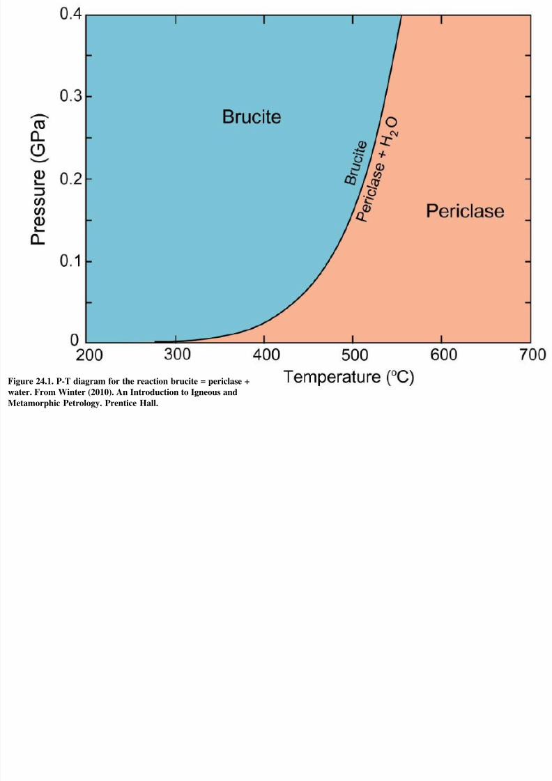
Consider the very simple metamorphic system, MgO-H2O
• Possible natural phases in this system are periclase
(MgO), aqueous fluid (H2O), and brucite (Mg(OH)2)
• How we deal with H2O depends upon whether water is
perfectly mobile or not
• A reaction can occur between the potential phases in this
system:
MgO + H2O Mg(OH)2 Per + Fluid = Bru

8/2/2019 Ch 24 Mineral Assemblages
http://slidepdf.com/reader/full/ch-24-mineral-assemblages 13/77
Figure 24.1. P-T diagram for the reaction brucite = periclase +water. From Winter (2010). An Introduction to Igneous and
Metamorphic Petrology. Prentice Hall.

8/2/2019 Ch 24 Mineral Assemblages
http://slidepdf.com/reader/full/ch-24-mineral-assemblages 14/77
8/2/2019 Ch 24 Mineral Assemblages
http://slidepdf.com/reader/full/ch-24-mineral-assemblages 15/77
Figure 24.1. P-T diagram for the reaction brucite = periclase +
water. From Winter (2010). An Introduction to Igneous and
Metamorphic Petrology. Prentice Hall.

8/2/2019 Ch 24 Mineral Assemblages
http://slidepdf.com/reader/full/ch-24-mineral-assemblages 16/77
The Phase Rule in Metamorphic Systems
How do you know which way is correct?
The rocks should tell you
• Phase rule = interpretive tool, not predictive
• If only see low-f assemblages (e.g. Per or Bru in the
MgO-H2O system) some components may be mobile
• If many phases in an area it is unlikely that all is right on
univariant curve, and may require the number of
components to include otherwise mobile phases, such as
H2O or CO2, in order to apply the phase rule correctly
8/2/2019 Ch 24 Mineral Assemblages
http://slidepdf.com/reader/full/ch-24-mineral-assemblages 17/77
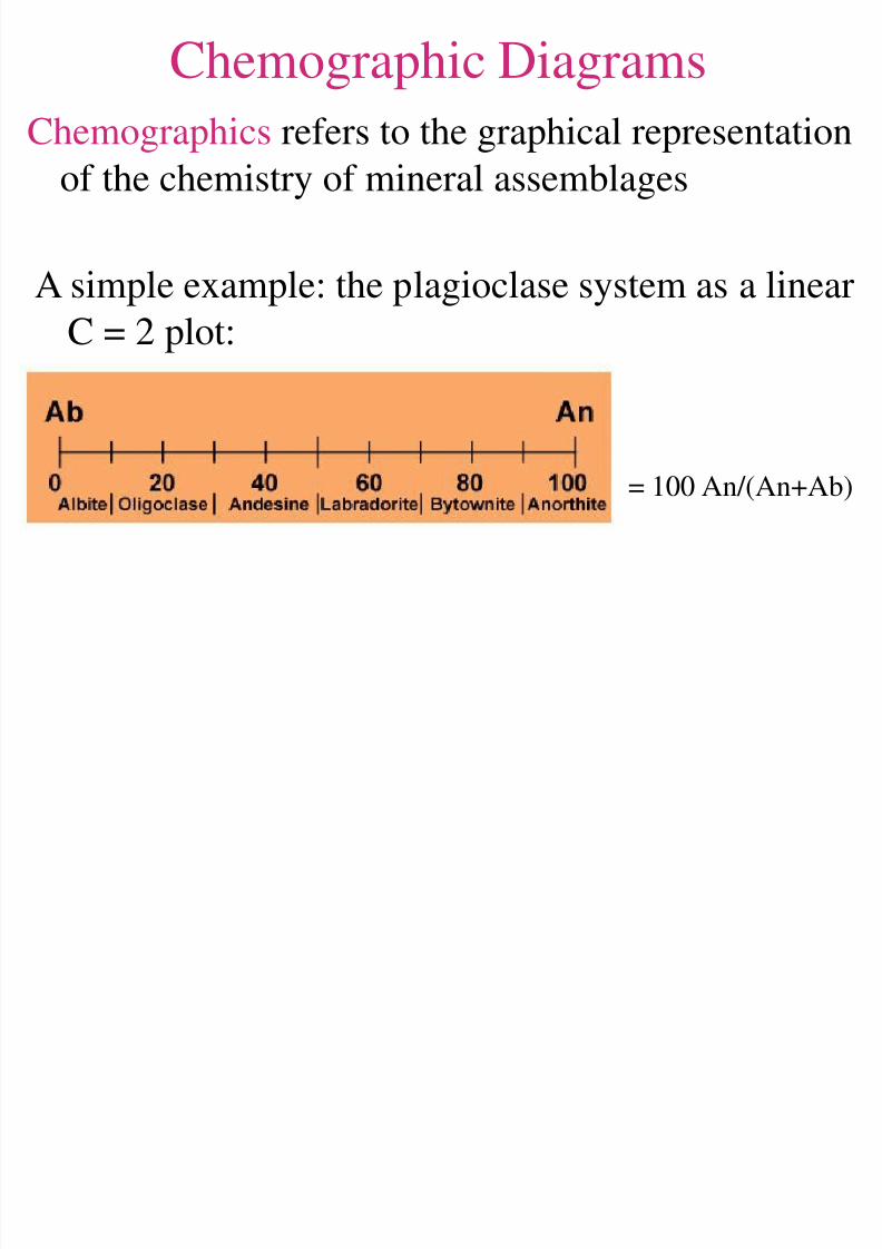
Chemographic Diagrams
Chemographics refers to the graphical representation
of the chemistry of mineral assemblages
A simple example: the plagioclase system as a linear
C = 2 plot:
= 100 An/(An+Ab)

8/2/2019 Ch 24 Mineral Assemblages
http://slidepdf.com/reader/full/ch-24-mineral-assemblages 18/77

8/2/2019 Ch 24 Mineral Assemblages
http://slidepdf.com/reader/full/ch-24-mineral-assemblages 19/77

8/2/2019 Ch 24 Mineral Assemblages
http://slidepdf.com/reader/full/ch-24-mineral-assemblages 20/77
Note that this subdivides the chemographic diagram into 5
sub-triangles, labeled (A)-(E)
x - xy - x2z
xy - xyz - x2zxy - xyz - y
xyz - z - x2z
y - z - xyz

8/2/2019 Ch 24 Mineral Assemblages
http://slidepdf.com/reader/full/ch-24-mineral-assemblages 21/77

8/2/2019 Ch 24 Mineral Assemblages
http://slidepdf.com/reader/full/ch-24-mineral-assemblages 22/77
What happens if you pick a composition that falls directly on
a tie-line, such as point (f)?
Figure 24.2. Hypothetical three-component
chemographic compatibility diagram
illustrating the positions of various stable
minerals. Minerals that coexist compatiblyunder the range of P-T conditions specific to
the diagram are connected by tie-lines. After
Best (1982) Igneous and Metamorphic
Petrology. W. H. Freeman.

8/2/2019 Ch 24 Mineral Assemblages
http://slidepdf.com/reader/full/ch-24-mineral-assemblages 23/77
In the unlikely event that the bulk
composition equals that of a single
mineral, such as xyz, then f = 1, but
C = 1 as well
“compositionally
degenerate”

8/2/2019 Ch 24 Mineral Assemblages
http://slidepdf.com/reader/full/ch-24-mineral-assemblages 24/77
Chemographic Diagrams
Valid compatibility diagram must be referenced to a
specific range of P-T conditions, such as a zone in
some metamorphic terrane, because the stability of
the minerals and their groupings vary as P and T vary
• Previous diagram refers to a P-T range in which
the fictitious minerals x, y, z, xy, xyz, and x2z are
all stable and occur in the groups shown
• At different grades the diagrams change
Other minerals become stable
Different arrangements of the same minerals (different
tie-lines connect different coexisting phases)
8/2/2019 Ch 24 Mineral Assemblages
http://slidepdf.com/reader/full/ch-24-mineral-assemblages 25/77
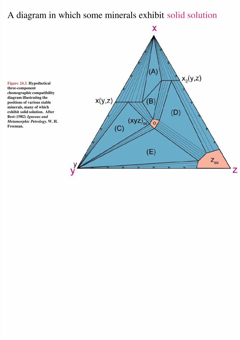
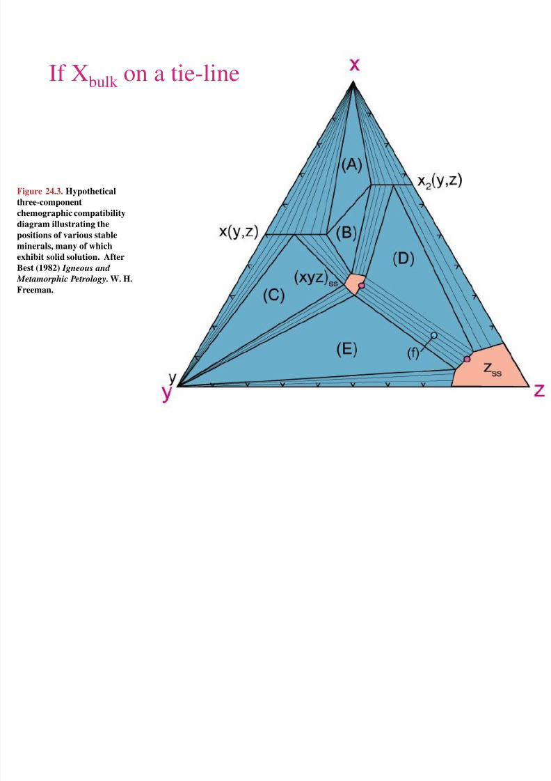
A diagram in which some minerals exhibit solid solution
Figure 24.3. Hypotheticalthree-component
chemographic compatibility
diagram illustrating the
positions of various stable
minerals, many of which
exhibit solid solution. After
Best (1982) Igneous and
Metamorphic Petrology. W. H.
Freeman.
8/2/2019 Ch 24 Mineral Assemblages
http://slidepdf.com/reader/full/ch-24-mineral-assemblages 26/77
Figure 24.3. Hypotheticalthree-component
chemographic compatibility
diagram illustrating the
positions of various stable
minerals, many of which
exhibit solid solution. After
Best (1982) Igneous and
Metamorphic Petrology. W. H.
Freeman.
If Xbulk on a tie-line

8/2/2019 Ch 24 Mineral Assemblages
http://slidepdf.com/reader/full/ch-24-mineral-assemblages 27/77
Xbulk in 3-phase triangles F = 2 (P & T) so Xmin fixed
Figure 24.3. Hypotheticalthree-component
chemographic compatibility
diagram illustrating the
positions of various stable
minerals, many of which
exhibit solid solution. After
Best (1982) Igneous and
Metamorphic Petrology. W. H.
Freeman.

8/2/2019 Ch 24 Mineral Assemblages
http://slidepdf.com/reader/full/ch-24-mineral-assemblages 28/77
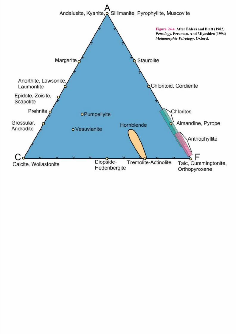
Chemographic Diagrams for
Metamorphic Rocks
• Most common natural rocks contain the major
elements: SiO2, Al2O3, K2O, CaO, Na2O, FeO,
MgO, MnO and H2O such that C = 9
• Three components is the maximum number that
we can easily deal with in two dimensions
•
What is the “right” choice of components?• Some simplifying methods:

8/2/2019 Ch 24 Mineral Assemblages
http://slidepdf.com/reader/full/ch-24-mineral-assemblages 29/77
1) Simply “ignore” components
• Trace elements
• Elements that enter only a single phase
(we can drop both the component and the
phase without violating the phase rule)
• Perfectly mobile components
8/2/2019 Ch 24 Mineral Assemblages
http://slidepdf.com/reader/full/ch-24-mineral-assemblages 30/77
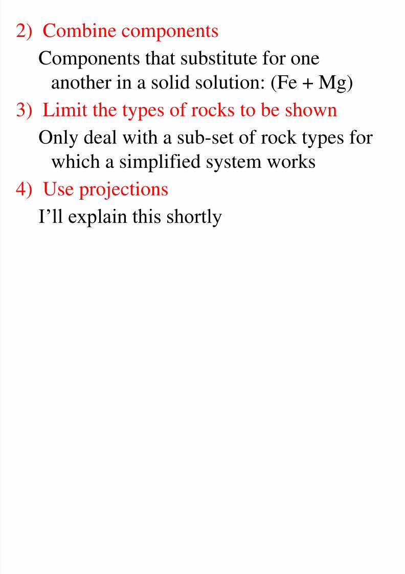
2) Combine components
Components that substitute for one
another in a solid solution: (Fe + Mg)
3) Limit the types of rocks to be shown
Only deal with a sub-set of rock types forwhich a simplified system works
4) Use projections
I’ll explain this shortly

8/2/2019 Ch 24 Mineral Assemblages
http://slidepdf.com/reader/full/ch-24-mineral-assemblages 31/77

8/2/2019 Ch 24 Mineral Assemblages
http://slidepdf.com/reader/full/ch-24-mineral-assemblages 32/77
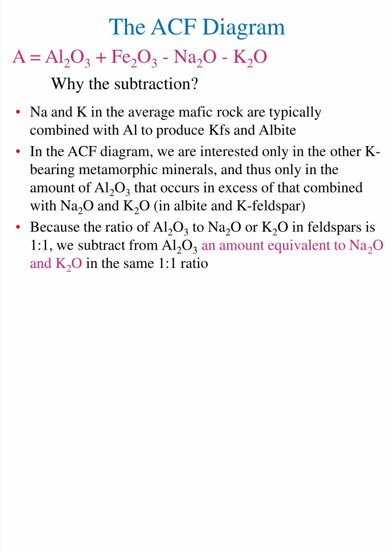
The ACF Diagram
• Illustrate metamorphic mineral assemblages in mafic rockson a simplified 3-C triangular diagram
• Concentrate only on the minerals that appeared or
disappeared during metamorphism, thus acting as
indicators of metamorphic grade
8/2/2019 Ch 24 Mineral Assemblages
http://slidepdf.com/reader/full/ch-24-mineral-assemblages 33/77

8/2/2019 Ch 24 Mineral Assemblages
http://slidepdf.com/reader/full/ch-24-mineral-assemblages 34/77
The ACF Diagram
The three pseudo-components are all calculated
on an atomic basis:
A = Al2O3 + Fe2O3 - Na2O - K2O
C = CaO - 3.3 P2O
5
F = FeO + MgO + MnO
8/2/2019 Ch 24 Mineral Assemblages
http://slidepdf.com/reader/full/ch-24-mineral-assemblages 35/77
The ACF Diagram
A = Al2O3 + Fe2O3 - Na2O - K2O
Why the subtraction?
• Na and K in the average mafic rock are typically
combined with Al to produce Kfs and Albite
• In the ACF diagram, we are interested only in the other K-
bearing metamorphic minerals, and thus only in the
amount of Al2O3 that occurs in excess of that combined
with Na2O and K2O (in albite and K-feldspar)• Because the ratio of Al2O3 to Na2O or K2O in feldspars is
1:1, we subtract from Al2O3 an amount equivalent to Na2O
and K2O in the same 1:1 ratio

8/2/2019 Ch 24 Mineral Assemblages
http://slidepdf.com/reader/full/ch-24-mineral-assemblages 36/77

8/2/2019 Ch 24 Mineral Assemblages
http://slidepdf.com/reader/full/ch-24-mineral-assemblages 37/77
The ACF Diagram
• Water is omitted under the assumption that it is perfectly
mobile
•
Note that SiO2 is simply ignored We shall see that this is equivalent to projecting from quartz
• In order for a projected phase diagram to be truly valid,
the phase from which it is projected must be present in the
mineral assemblages represented
By creating these three pseudo-components, Eskola reduced
the number of components in mafic rocks from 8 to 3

8/2/2019 Ch 24 Mineral Assemblages
http://slidepdf.com/reader/full/ch-24-mineral-assemblages 38/77

8/2/2019 Ch 24 Mineral Assemblages
http://slidepdf.com/reader/full/ch-24-mineral-assemblages 39/77

8/2/2019 Ch 24 Mineral Assemblages
http://slidepdf.com/reader/full/ch-24-mineral-assemblages 40/77
A typical ACF compatibility diagram, referring to a specific
range of P and T (the kyanite zone in the Scottish Highlands)
Figure 24.5. After
Turner (1981).
Metamorphic Petrology.
M cGraw Hill.

8/2/2019 Ch 24 Mineral Assemblages
http://slidepdf.com/reader/full/ch-24-mineral-assemblages 41/77

8/2/2019 Ch 24 Mineral Assemblages
http://slidepdf.com/reader/full/ch-24-mineral-assemblages 42/77

8/2/2019 Ch 24 Mineral Assemblages
http://slidepdf.com/reader/full/ch-24-mineral-assemblages 43/77
AKF compatibility diagram (Eskola, 1915) illustrating
paragenesis of pelitic hornfelses, Orijärvi region Finland
Figure 24.7. AfterEskola (1915) and
Turner (1981)
Metamorphic Petrology.
M cGraw Hill.

8/2/2019 Ch 24 Mineral Assemblages
http://slidepdf.com/reader/full/ch-24-mineral-assemblages 44/77

8/2/2019 Ch 24 Mineral Assemblages
http://slidepdf.com/reader/full/ch-24-mineral-assemblages 45/77
8/2/2019 Ch 24 Mineral Assemblages
http://slidepdf.com/reader/full/ch-24-mineral-assemblages 46/77

8/2/2019 Ch 24 Mineral Assemblages
http://slidepdf.com/reader/full/ch-24-mineral-assemblages 47/77
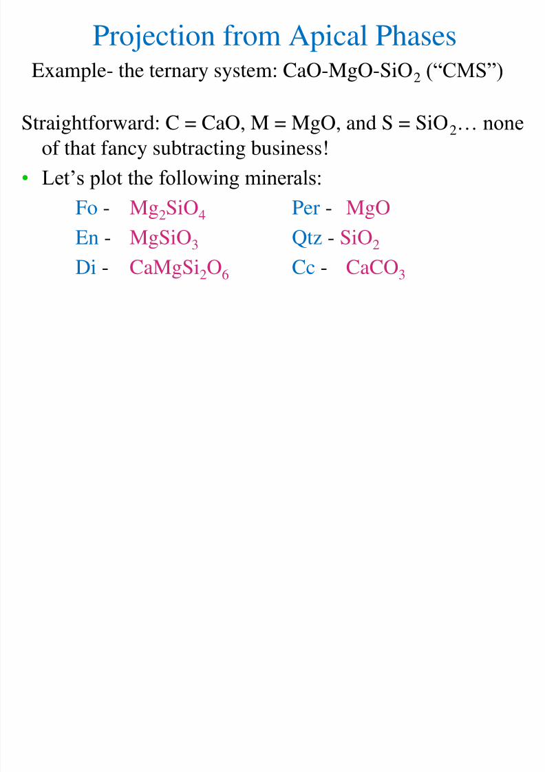
Projection from Apical PhasesFo - Mg2SiO4 Per - MgO En - MgSiO3
Qtz - SiO2 Di - CaMgSi2O6 Cc - CaCO3

8/2/2019 Ch 24 Mineral Assemblages
http://slidepdf.com/reader/full/ch-24-mineral-assemblages 48/77

8/2/2019 Ch 24 Mineral Assemblages
http://slidepdf.com/reader/full/ch-24-mineral-assemblages 49/77
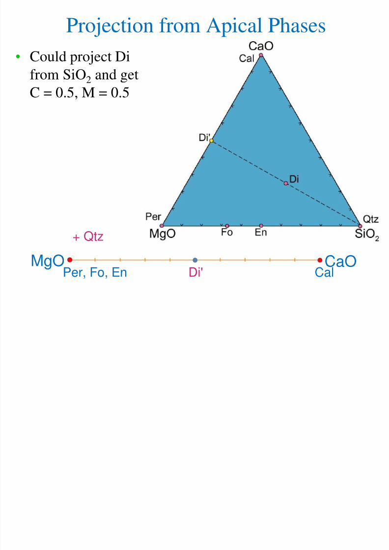
Projection from Apical Phases
Pseudo-binary Mg-Si diagram in which Di is
projected to a 33% Mg - 66% Si
MgO SiO 2 Fo En Di' Q Per
+ Cal
Fo - Mg2SiO4 Per - MgO En - MgSiO3
Qtz - SiO2 Di - CaMgSi2O6 Cc - CaCO3
8/2/2019 Ch 24 Mineral Assemblages
http://slidepdf.com/reader/full/ch-24-mineral-assemblages 50/77

8/2/2019 Ch 24 Mineral Assemblages
http://slidepdf.com/reader/full/ch-24-mineral-assemblages 51/77
Projection from Apical Phases
• In accordance with the mineralogical phase rule
(f = C) get any of the following 2-phase mineral
assemblages in our 2-component system:
Per + Fo Fo + En
En + Di Di + Q
MgO SiO 2 Fo En Di' Q Per
Projection from Apical Phases
8/2/2019 Ch 24 Mineral Assemblages
http://slidepdf.com/reader/full/ch-24-mineral-assemblages 52/77
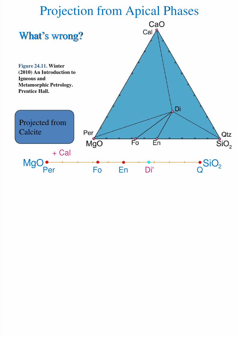
Projection from Apical Phases
What’s wrong?
MgO SiO 2 Fo En Di' Q Per
Figure 24.11. Winter
(2010) An Introduction to
Igneous and
Metamorphic Petrology.Prentice Hall.
Projected from
Calcite
+ Cal
Projection from Apical Phases

8/2/2019 Ch 24 Mineral Assemblages
http://slidepdf.com/reader/full/ch-24-mineral-assemblages 53/77
Projection from Apical Phases
What’s wrong?
MgO SiO 2 Fo En
+ Di
Q Per
Figure 24.11. Winter
(2010) An Introduction to
Igneous and
Metamorphic Petrology.Prentice Hall.
Better to have
projected fromDiopside

8/2/2019 Ch 24 Mineral Assemblages
http://slidepdf.com/reader/full/ch-24-mineral-assemblages 54/77
P j i f A i l Ph
8/2/2019 Ch 24 Mineral Assemblages
http://slidepdf.com/reader/full/ch-24-mineral-assemblages 55/77
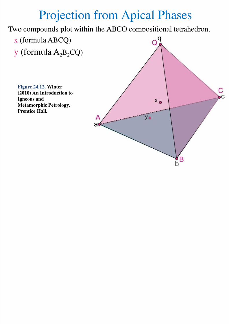
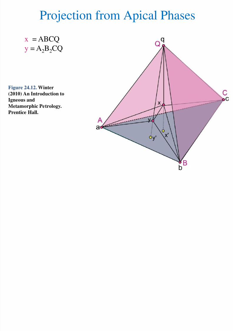
Projection from Apical PhasesTwo compounds plot within the ABCQ compositional tetrahedron,
x (formula ABCQ)y (formula A2B2CQ)
Figure 24.12. Winter
(2010) An Introduction to
Igneous and
Metamorphic Petrology.
Prentice Hall.
P j i f A i l Ph

8/2/2019 Ch 24 Mineral Assemblages
http://slidepdf.com/reader/full/ch-24-mineral-assemblages 56/77
Projection from Apical Phases
Figure 24.12. Winter
(2010) An Introduction to
Igneous and
Metamorphic Petrology.
Prentice Hall.
x = ABCQ
y = A2B2CQ
P j i f A i l Ph
8/2/2019 Ch 24 Mineral Assemblages
http://slidepdf.com/reader/full/ch-24-mineral-assemblages 57/77
Figure 24.12. Winter
(2010) An Introduction to
Igneous and
Metamorphic Petrology.
Prentice Hall.
Projection from Apical Phases
x = ABCQ
y = A2B2CQ
P j ti f A i l Ph

8/2/2019 Ch 24 Mineral Assemblages
http://slidepdf.com/reader/full/ch-24-mineral-assemblages 58/77
Projection from Apical Phasesx plots as x' since A:B:C = 1:1:1 = 33:33:33
y plots as y' since A:B:C = 2:2:1 = 40:40:20
Figure 24.13. Winter
(2010) An Introduction to
Igneous and
Metamorphic Petrology.
Prentice Hall.
x = ABCQ
y = A2B2CQ
P j ti f A i l Ph

8/2/2019 Ch 24 Mineral Assemblages
http://slidepdf.com/reader/full/ch-24-mineral-assemblages 59/77
Projection from Apical Phases
If we remember our projection
point (q), we conclude from thisdiagram that the following
assemblages are possible:
(q)-b-x-c
(q)-a-x-y(q)-b-x-y
(q)-a-b-y
(q)-a-x-c
The assemblage a-b-c
appears to be impossible
P j ti f A i l Ph

8/2/2019 Ch 24 Mineral Assemblages
http://slidepdf.com/reader/full/ch-24-mineral-assemblages 60/77
Projection from Apical Phases
Figure 24.12. Winter
(2010) An Introduction to
Igneous and
Metamorphic Petrology.
Prentice Hall.
P j ti f A i l Ph

8/2/2019 Ch 24 Mineral Assemblages
http://slidepdf.com/reader/full/ch-24-mineral-assemblages 61/77
Projection from Apical Phases
J B Th ’ A(K)FM Di

8/2/2019 Ch 24 Mineral Assemblages
http://slidepdf.com/reader/full/ch-24-mineral-assemblages 62/77
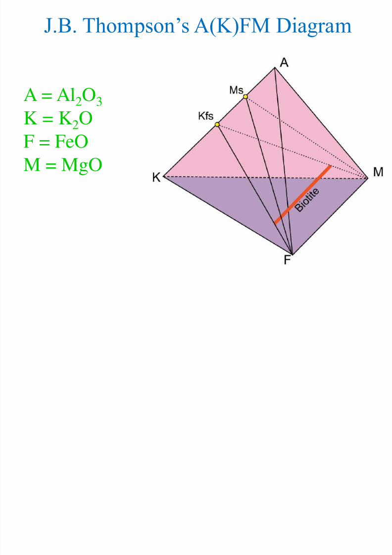
J.B. Thompson’s A(K)FM Diagram
An alternative to the AKF diagram for metamorphosed
pelitic rocks
Although the AKF is useful in this capacity, J.B.
Thompson (1957) noted that Fe and Mg do not
partition themselves equally between the variousmafic minerals in most rocks
J B Th ’ A(K)FM Di

8/2/2019 Ch 24 Mineral Assemblages
http://slidepdf.com/reader/full/ch-24-mineral-assemblages 63/77
J.B. Thompson’s A(K)FM Diagram
Figure 24.17. Partitioning of
Mg/Fe in minerals in ultramafic
rocks, Bergell aureole, Italy
After Trommsdorff and Evans
(1972). A J Sci 272, 423-437.
J B Th ’ A(K)FM Di
8/2/2019 Ch 24 Mineral Assemblages
http://slidepdf.com/reader/full/ch-24-mineral-assemblages 64/77
J.B. Thompson’s A(K)FM Diagram
A = Al2O3
K = K2O
F = FeOM = MgO
J B Thompson’s

8/2/2019 Ch 24 Mineral Assemblages
http://slidepdf.com/reader/full/ch-24-mineral-assemblages 65/77
J.B. Thompson sA(K)FM
Diagram
Project from a phase that is
present in the mineral
assemblages to be studied
Figure 24.18. AKFM Projection
from Mu. After Thompson (1957).
Am. Min. 22, 842-858.
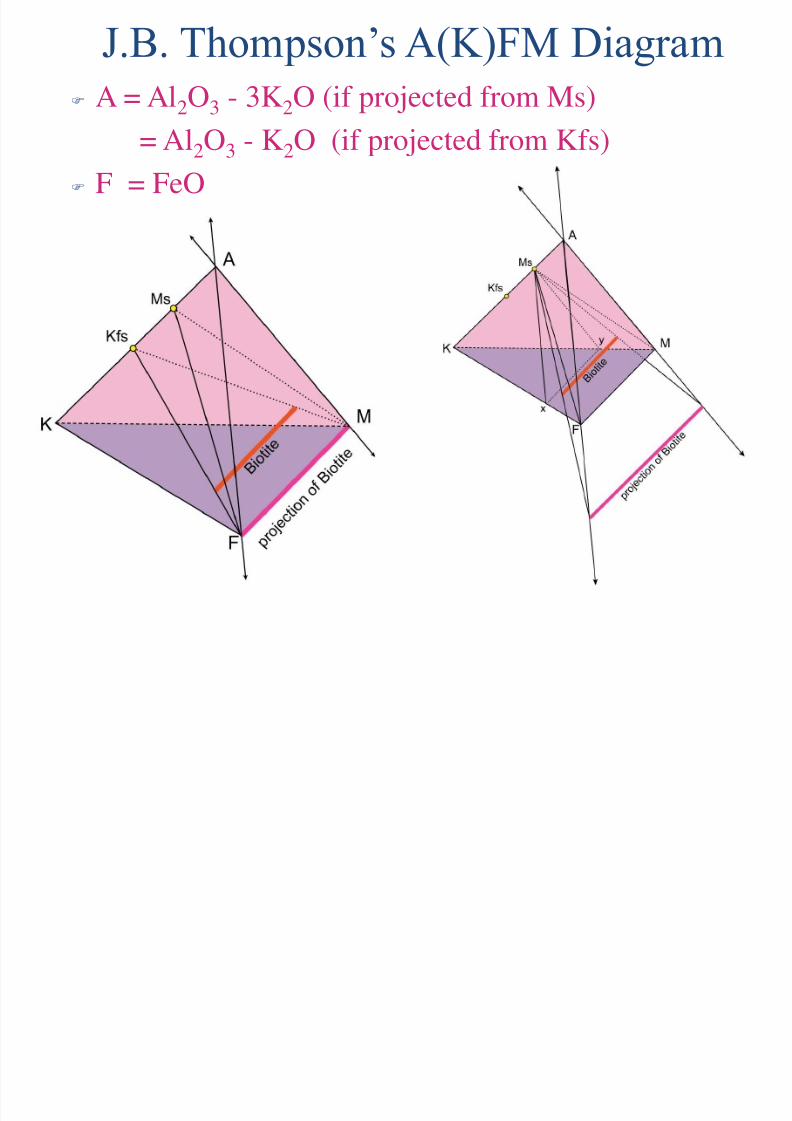
J B Thompson’s A(K)FM Diagram

8/2/2019 Ch 24 Mineral Assemblages
http://slidepdf.com/reader/full/ch-24-mineral-assemblages 66/77
J.B. Thompson’s A(K)FM Diagram
• At high grades muscovite
dehydrates to K-feldspar as thecommon high-K phase
• Then the AFM diagram should
be projected from K-feldspar
• When projected from Kfs,biotite projects within the F-M
base of the AFM triangle
Figure 24.18. AKFM Projection
from Kfs. After Thompson (1957).
Am. Min. 22, 842-858.
J B Thompson’s A(K)FM Diagram
8/2/2019 Ch 24 Mineral Assemblages
http://slidepdf.com/reader/full/ch-24-mineral-assemblages 67/77
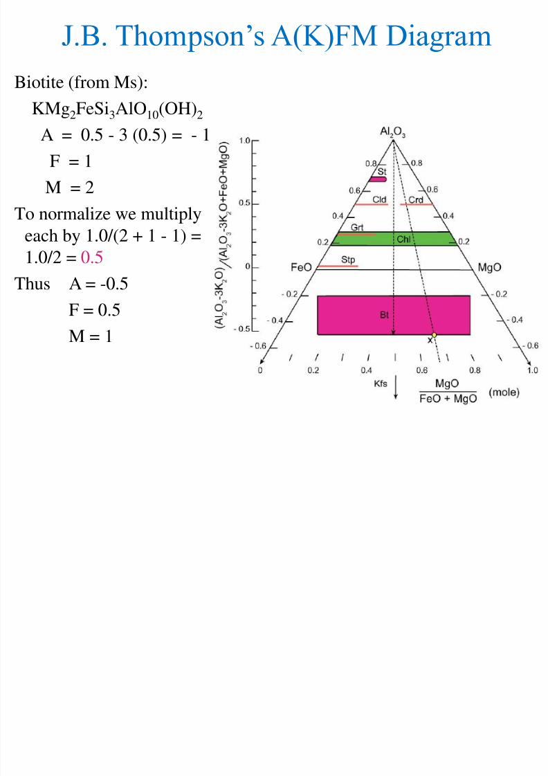
J.B. Thompson s A(K)FM Diagram
A = Al2O3 - 3K2O (if projected from Ms)
= Al2O3 - K2O (if projected from Kfs) F = FeO
M = MgO
J B Thompson’s A(K)FM Diagram
8/2/2019 Ch 24 Mineral Assemblages
http://slidepdf.com/reader/full/ch-24-mineral-assemblages 68/77
J.B. Thompson s A(K)FM Diagram
Biotite (from Ms):
KMg2FeSi3AlO10(OH)2
A = 0.5 - 3 (0.5) = - 1
F = 1
M = 2
To normalize we multiply
each by 1.0/(2 + 1 - 1) =
1.0/2 = 0.5
Thus A = -0.5
F = 0.5
M = 1
J B Thompson’s A(K)FM Diagram
8/2/2019 Ch 24 Mineral Assemblages
http://slidepdf.com/reader/full/ch-24-mineral-assemblages 69/77
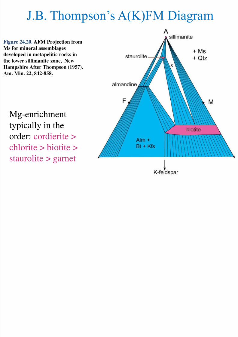
J.B. Thompson s A(K)FM Diagram
Figure 24.20. AFM Projection from
Ms for mineral assemblages
developed in metapelitic rocks in
the lower sillimanite zone, New
Hampshire After Thompson (1957).
Am. Min. 22, 842-858.
Mg-enrichment
typically in theorder: cordierite >
chlorite > biotite >
staurolite > garnet
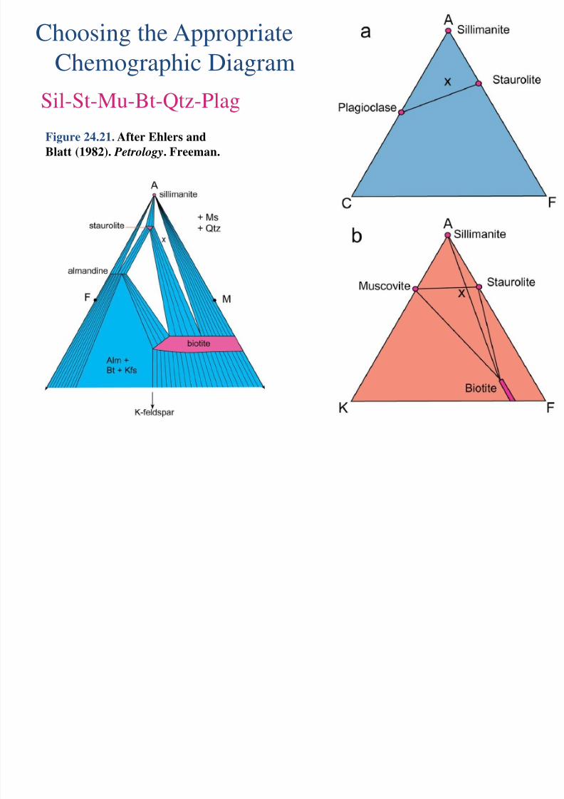
Choosing the Appropriate Chemographic Diagram

8/2/2019 Ch 24 Mineral Assemblages
http://slidepdf.com/reader/full/ch-24-mineral-assemblages 70/77
Choosing the Appropriate Chemographic Diagram
• Example, suppose we have a series of pelitic rocks in
an area. The pelitic system consists of the 9 principalcomponents: SiO2, Al2O3, FeO, MgO, MnO, CaO,
Na2O, K2O, and H2O
• How do we lump those 9 components to get ameaningful and useful diagram?
Choosing the Appropriate Chemographic Diagram

8/2/2019 Ch 24 Mineral Assemblages
http://slidepdf.com/reader/full/ch-24-mineral-assemblages 71/77
Choosing the Appropriate Chemographic Diagram
Each simplifying step makes the resulting system easier to
visualize, but may overlook some aspect of the rocks inquestion
• MnO is commonly lumped with FeO + MgO, or
ignored, as it usually occurs in low concentrations andenters solid solutions along with FeO and MgO
• In metapelites Na2O is usually significant only in
plagioclase, so we may often ignore it, or project from
albite• As a rule, H2O is sufficiently mobile to be ignored as
well
Choosing the Appropriate Chemographic Diagram

8/2/2019 Ch 24 Mineral Assemblages
http://slidepdf.com/reader/full/ch-24-mineral-assemblages 72/77
Choosing the Appropriate Chemographic Diagram
Common high-grade mineral assemblage:
Sil-St-Mu-Bt-Qtz-Plag
Figure 24.20. AFM Projection from
Ms for mineral assemblages
developed in metapelitic rocks in
the lower sillimanite zone, New
Hampshire After Thompson (1957).
Am. Min. 22, 842-858.
Choosing the Appropriate
8/2/2019 Ch 24 Mineral Assemblages
http://slidepdf.com/reader/full/ch-24-mineral-assemblages 73/77
Choosing the Appropriate
Chemographic Diagram
Figure 24.21. After Ehlers and
Blatt (1982). Petrology. Freeman.
Sil-St-Mu-Bt-Qtz-Plag
Choosing the Appropriate Chemographic Diagram

8/2/2019 Ch 24 Mineral Assemblages
http://slidepdf.com/reader/full/ch-24-mineral-assemblages 74/77
Choosing the Appropriate Chemographic Diagram
We don’t have equilibrium
There is a reaction taking
place (F = 1)
We haven’t chosen our components correctly and
we do not really have 3
components in terms of AKF
Figure 24.21. After Ehlers and
Blatt (1982). Petrology. Freeman.
Sil-St-Mu-Bt-Qtz-Plag
Choosing the Appropriate Chemographic Diagram

8/2/2019 Ch 24 Mineral Assemblages
http://slidepdf.com/reader/full/ch-24-mineral-assemblages 75/77
Choosing the Appropriate Chemographic Diagram
Figure 24.21. After Ehlers and
Blatt (1982). Petrology. Freeman.
Sil-St-Mu-Bt-Qtz-Plag
Choosing the Appropriate Chemographic Diagram

8/2/2019 Ch 24 Mineral Assemblages
http://slidepdf.com/reader/full/ch-24-mineral-assemblages 76/77
Choosing the Appropriate Chemographic Diagram
• Myriad chemographic diagrams have been proposed to
analyze paragenetic relationships in variousmetamorphic rock types
• Most are triangular: the maximum number that can be
represented easily and accurately in two dimensions
• Some natural systems may conform to a simple 3-
component system, and the resulting metamorphic
phase diagram is rigorous in terms of the mineral
assemblages that develop• Other diagrams are simplified by combining
components or projecting
Choosing the Appropriate Chemographic Diagram

8/2/2019 Ch 24 Mineral Assemblages
http://slidepdf.com/reader/full/ch-24-mineral-assemblages 77/77
Choosing the Appropriate Chemographic Diagram
• Variations in metamorphic mineral assemblages result
from:1) Differences in bulk chemistry
2) differences in intensive variables, such as T, P, PH2O,
etc (metamorphic grade)
• A good chemographic diagram permits easy
visualization of the first situation
• The second can be determined by a balanced reaction in
which one rock’s mineral assemblage contains thereactants and another the products
• These differences can often be visualized by comparing
h hi di f h d


