Download - Chapter 1 Quality Improvement in the Modern Business ... Manual for Introduction to Statistical Quality... · Armand V. Feigenbaum 6. Discuss total quality management, the Malcolm

Chapter 1

Quality Improvement in the Modern Business Environment

LEARNING OBJECTIVES

After completing this chapter you should be able to:

1. Define and discuss quality and quality improvement 2. Discuss the different dimensions of quality 3. Discuss the evolution of modern quality improvement methods 4. Discuss the role that variability and statistical methods play in controlling and improving quality 5. Describe the quality management philosophies of W. Edwards Deming, Joseph M. Juran, and

Armand V. Feigenbaum 6. Discuss total quality management, the Malcolm Baldrige National Quality Award, Six-Sigma, and

quality systems and standards 7. Explain the links between quality and productivity and between quality and cost 8. Discuss product liability 9. Discuss the three functions: quality planning, quality assurance, and quality control and

improvement

IMPORTANT TERMS AND CONCEPTS

Acceptance sampling Quality control and improvement

Appraisal costs Quality engineering

Deming’s 14 points Quality of conformance

Designed experiments Quality of design

Dimensions of quality Quality planning

Fitness for use Quality systems and standards

Internal and External failure costs Six-Sigma

ISO 9000:2005 Specifications

Nonconforming product or service Statistical process control (SPC)

Prevention costs The Juran Trilogy

Product liability The Malcolm Baldrige National Quality Award

Quality assurance Total quality management (TQM)

Quality characteristics Variability

1-2 CHAPTER 1 QUALITY IMPROVEMENT IN THE MODERN BUSINESS ENVIRONMENT

COMMENTS

The modern definition of quality, “Quality is inversely proportional to variability” (text p. 6), implies that

product quality increases as variability in important product characteristics decreases. Quality

improvement can then be defined as “… the reduction of variability in processes and products” (text p.

7). Since the early 1900’s, statistical methods have been used to control and improve quality. In the

Introduction to Statistical Quality Control, 7th ed., by Douglas C. Montgomery, methods applicable in

the key areas of process control, design of experiments, and acceptance sampling are presented.

To understand the potential for application of statistical methods, it may help to envision the system

that creates a product as a “black box” (text Figure 1-3). The output of this black box is a product whose

quality is defined by one or more quality characteristics that represent dimensions such as conformance

to standards, performance, or reliability. Product quality can be evaluated with acceptance sampling

plans. These plans are typically applied to either the output of a process or the input raw materials and

components used in manufacturing. Application of process control techniques (such as control charts)

or statistically designed experiments can achieve significant reduction in variability.

Black box inputs are categorized as “incoming raw materials and parts,” “controllable inputs,” and

“uncontrollable inputs.”

The quality of incoming raw materials and parts is often assessed with acceptance sampling plans. As

material is received from suppliers, incoming lots are inspected then dispositioned as either acceptable

or unacceptable. Once a history of high quality material is established, a customer may accept the

supplier’s process control data in lieu of incoming inspection results.

“Controllable” and “uncontrollable” inputs apply to incoming materials, process variables, and

environmental factors. For example, it may be difficult to control the temperature in a heat-treating

oven in the sense that some areas of the oven may be cooler while some areas may be warmer.

Properties of incoming materials may be very difficult to control. For example, the moisture content

and proportion of hardwood in trees used for papermaking have a significant impact on the quality

characteristics of the finished paper. Environmental variables such as temperature and relative

humidity are often hard to control precisely.

Whether or not controllable and uncontrollable inputs are significant can be determined through

process characterization. Statistically designed experiments are extremely helpful in characterizing

processes and optimizing the relationship between incoming materials, process variables, and product

characteristics.

CHAPTER 1 QUALITY IMPROVEMENT IN THE MODERN BUSINESS ENVIRONMENT 1-3

Although the initial tendency is to think of manufacturing processes and products, the statistical

methods presented in this text can also be applied to business processes and products, such as financial

transactions and services. In some organizations the opportunity to improve quality in three areas is

even greater than it is in manufacturing.

Various quality philosophies and management systems are briefly described in the text; a common

thread is the necessity for continuous improvement to increase productivity and reduce cost. The

technical tools described in the text are essential for successful quality improvement. Quality

management systems alone do not reduce variability and improve quality.

Chapter 2

The DMAIC Process

LEARNING OBJECTIVES


1. Understand the importance of selecting good projects for improvement activities

2. Explain the five steps of DMAIC: Define, Measure, Analyze, Improve, and Control

3. Explain the purpose of tollgate reviews

4. Understand the decision-making requirements of the tollgate review for each DMAIC step

5. Know when and when not to use DMAIC

6. Understand how DMAIC fits into the framework of the Six Sigma philosophy


Analyze step Key process input variables (KPIV)

Control step Key process output variables (KPOV)

Define step Measure step

Design for Six Sigma (DFSS) Project charter

DMAIC SIPOC diagram

Failure modes and effects analysis (FMEA) Six Sigma

Improve step Tollgate

2-2 CHAPTER 2 THE DMAIC PROCESS

EXERCISES

2.7. Explain the importance of tollgates in the DMAIC process.

At a tollgate, a project team presents its work to managers and “owners” of the process. In a six-sigma

organization, the tollgate participants also would include the project champion, master black belts, and

other black belts not working directly on the project. Tollgates are where the project is reviewed to

ensure that it is on track and they provide a continuing opportunity to evaluate whether the team can

successfully complete the project on schedule. Tollgates also present an opportunity to provide

guidance regarding the use of specific technical tools and other information about the problem.

Organization problems and other barriers to success—and strategies for dealing

with them—also often are identified during tollgate reviews. Tollgates are critical to the overall

problem-solving process; It is important that these reviews be conducted very soon after the team

completes each step.

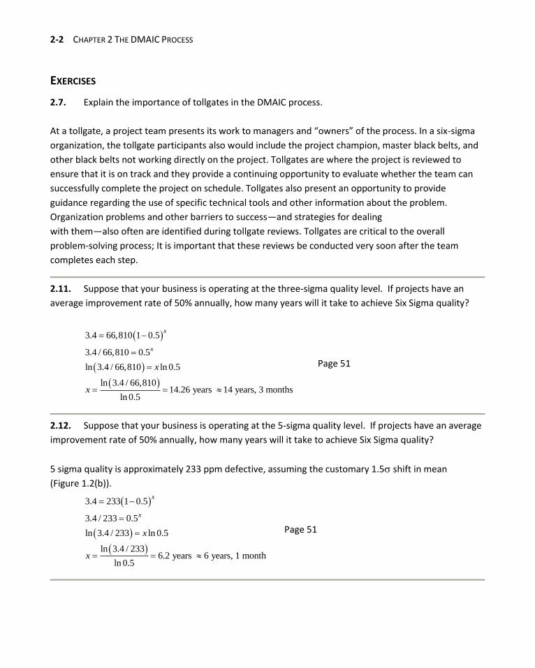
2.11. Suppose that your business is operating at the three-sigma quality level. If projects have an

average improvement rate of 50% annually, how many years will it take to achieve Six Sigma quality?

3.4 66,810 1 0.5

3.4 / 66,810 0.5

ln 3.4 / 66,810 ln 0.5

ln 3.4 / 66,81014.26 years 14 years, 3 months

ln 0.5

x

x

x

x

1

2.12. Suppose that your business is operating at the 5-sigma quality level. If projects have an average

improvement rate of 50% annually, how many years will it take to achieve Six Sigma quality?

5 sigma quality is approximately 233 ppm defective, assuming the customary 1.5 shift in mean

(Figure 1.2(b)).

3.4 233 1 0.5

3.4 / 233 0.5

ln 3.4 / 233 ln 0.5

ln 3.4 / 2336.2 years 6 years, 1 month

ln 0.5

x

x

x

x

Page 51

CHAPTER 2 THE DMAIC PROCESS 2-3

2.13. Explain why it is important to separate sources of variability into special or assignable causes

and common or chance causes.

Common or chance causes are due to the inherent variability in the system and cannot generally be

controlled. Special or assignable causes can be discovered and removed, thus reducing the variability in

the overall system. It is important to distinguish between the two types of variability, because the

strategy to reduce variability depends on the source. Chance cause variability can only be removed by

changing the system, while assignable cause variability can be addressed by finding and eliminating the

assignable causes.

2.15. Suppose that during the analyze phase an obvious solution is discovered. Should that solution

be immediately implemented and the remaining steps of DMAIC abandoned? Discuss your answer.

Generally, no. The advantage of completing the rest of the DMAIC process is that the solution will be

documented, tested, and it’s applicability to other parts of the business will be evaluated. An immediate

implementation of an “obvious” solution may not lead to an appropriate control plan. Completing the

rest of DMAIC can also lead to further refinements and improvements to the solution.

2.18. It has been estimated that safe aircraft carrier landings operate at about the 5 level. What

level of ppm defective does this imply?

If the operating limits are around the 5 level, and we assume the 1.5 shift in the mean customary for

Six Sigma applications, then the probability of a safe landing is the area under the normal curve that is

within 5 of the target mean, given that the true mean is 1.5 off of the target mean. Thus, the

probability of a safe landing is 0.999767 and the corresponding ppm defective is (1 − 0.999767)

1,000,000 = 233.

Chapter 3

Modeling Process Quality

LEARNING OBJECTIVES


1. Construct and interpret visual data displays, including the stem-and-leaf plot, the histogram, and

the box plot

2. Compute and interpret the sample mean, the sample variance, the sample standard deviation,

and the sample range

3. Explain the concepts of a random variable and a probability distribution

4. Understand and interpret the mean, variance, and standard deviation of a probability

distribution

5. Determine probabilities from probability distributions

6. Understand the assumptions for each of the discrete probability distributions presented

7. Understand the assumptions for each of the continuous probability distributions presented

8. Select an appropriate probability distribution

9. Use probability plots

10. Use approximations for some hypergeometric and binomial distributions


Approximations to probability distributions Percentile

Binomial distribution Poisson distribution

Box plot Population

Central limit theorem Probability distribution

Continuous distribution Probability plotting

Descriptive statistics Quartile

Discrete distribution Random variable

Exponential distribution Run chart

Gamma distribution Sample

Geometric distribution Sample average

Histogram Sample standard deviation

Hypergeometric probability distribution Sample variance

Interquartile range Standard deviation

3-2 CHAPTER 3 MODELING PROCESS QUALITY

Lognormal distribution Standard normal distribution

Mean of a distribution Statistics

Median Stem-and-leaf display

Negative binomial distribution Time series plot

Normal distribution Uniform distribution

Normal probability plot Variance of a distribution

Pascal distribution Weibull distribution

EXERCISES

New exercises are marked with .

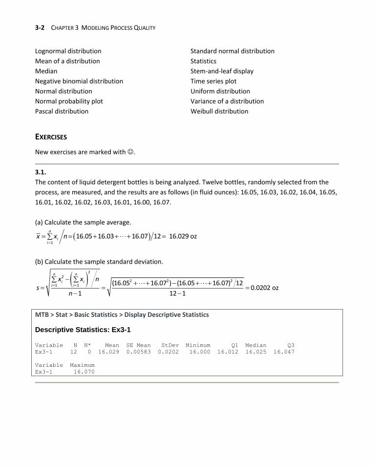
3.1.

The content of liquid detergent bottles is being analyzed. Twelve bottles, randomly selected from the

process, are measured, and the results are as follows (in fluid ounces): 16.05, 16.03, 16.02, 16.04, 16.05,

16.01, 16.02, 16.02, 16.03, 16.01, 16.00, 16.07.

(a) Calculate the sample average.

1

16.05 16.03 16.07 12 16.029 ozn

ii

x x n

(b) Calculate the sample standard deviation.

2

22 2 2

1 1 (16.05 16.07 ) (16.05 16.07) 120.0202 oz

1 12 1

n n

i ii i

x x ns

n

MTB > Stat > Basic Statistics > Display Descriptive Statistics

Descriptive Statistics: Ex3-1 Variable N N* Mean SE Mean StDev Minimum Q1 Median Q3

Ex3-1 12 0 16.029 0.00583 0.0202 16.000 16.012 16.025 16.047

Variable Maximum

Ex3-1 16.070

CHAPTER 3 MODELING PROCESS QUALITY 3-3

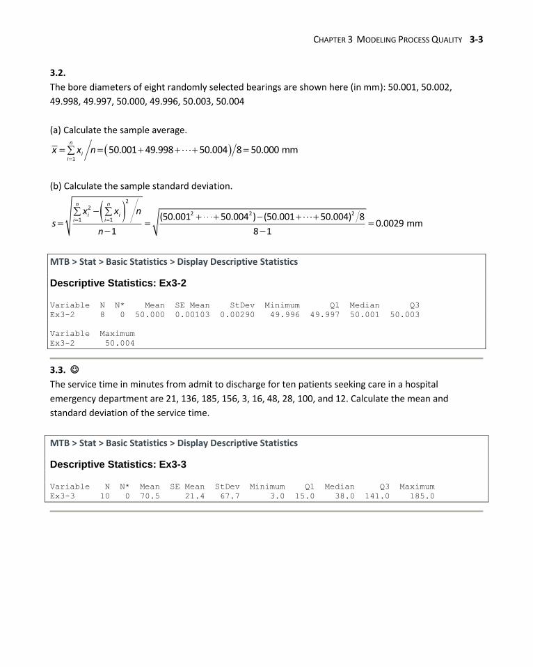
3.2.

The bore diameters of eight randomly selected bearings are shown here (in mm): 50.001, 50.002,

49.998, 49.997, 50.000, 49.996, 50.003, 50.004


1

50.001 49.998 50.004 8 50.000 mmn

ii

x x n


2

22 2 2

1 1 (50.001 50.004 ) (50.001 50.004) 80.0029 mm

1 8 1

n n

i ii i

x x ns

n



Ex3-2 8 0 50.000 0.00103 0.00290 49.996 49.997 50.001 50.003

Variable Maximum

Ex3-2 50.004

3.3.

The service time in minutes from admit to discharge for ten patients seeking care in a hospital

emergency department are 21, 136, 185, 156, 3, 16, 48, 28, 100, and 12. Calculate the mean and

standard deviation of the service time.


Descriptive Statistics: Ex3-3 Variable N N* Mean SE Mean StDev Minimum Q1 Median Q3 Maximum

Ex3-3 10 0 70.5 21.4 67.7 3.0 15.0 38.0 141.0 185.0


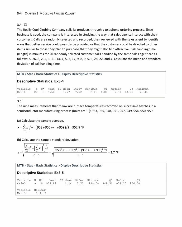
3.4.

The Really Cool Clothing Company sells its products through a telephone ordering process. Since

business is good, the company is interested in studying the way that sales agents interact with their

customers. Calls are randomly selected and recorded, then reviewed with the sales agent to identify

ways that better service could possibly be provided or that the customer could be directed to other

items similar to those they plan to purchase that they might also find attractive. Call handling time

(length) in minutes for 20 randomly selected customer calls handled by the same sales agent are as

follows: 5, 26, 8, 2, 5, 3, 11, 14, 4, 5, 2, 17, 9, 8, 9, 5, 3, 28, 22, and 4. Calculate the mean and standard

deviation of call handling time.


Descriptive Statistics: Ex3-4 Variable N N* Mean SE Mean StDev Minimum Q1 Median Q3 Maximum

Ex3-4 20 0 9.50 1.77 7.92 2.00 4.00 6.50 13.25 28.00

3.5.

The nine measurements that follow are furnace temperatures recorded on successive batches in a

semiconductor manufacturing process (units are °F): 953, 955, 948, 951, 957, 949, 954, 950, 959


1

953 955 959 9 952.9 °Fn

ii

x x n


2

22 2 2

1 1 (953 959 ) (953 959) 93.7 °F

1 9 1

n n

i ii i

x x ns

n



Ex3-5 9 0 952.89 1.24 3.72 948.00 949.50 953.00 956.00

Variable Maximum

Ex3-5 959.00


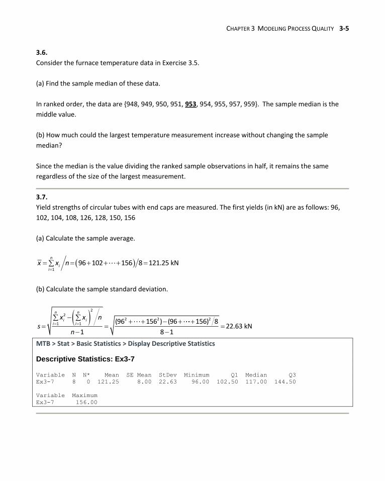
3.6.

Consider the furnace temperature data in Exercise 3.5.

(a) Find the sample median of these data.

In ranked order, the data are {948, 949, 950, 951, 953, 954, 955, 957, 959}. The sample median is the

middle value.

(b) How much could the largest temperature measurement increase without changing the sample

median?

Since the median is the value dividing the ranked sample observations in half, it remains the same

regardless of the size of the largest measurement.

3.7.

Yield strengths of circular tubes with end caps are measured. The first yields (in kN) are as follows: 96,

102, 104, 108, 126, 128, 150, 156


1

96 102 156 8 121.25 kNn

ii

x x n


2

22 2 2

1 1 (96 156 ) (96 156) 822.63 kN

1 8 1

n n

i ii i

x x ns

n



Ex3-7 8 0 121.25 8.00 22.63 96.00 102.50 117.00 144.50

Variable Maximum

Ex3-7 156.00


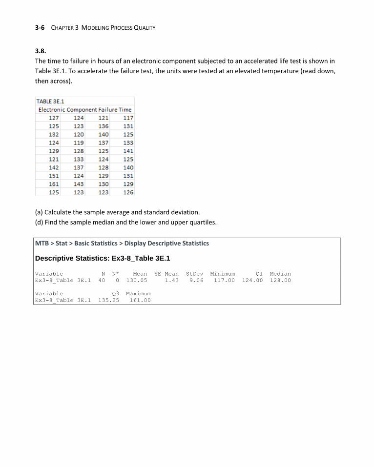
3.8.

The time to failure in hours of an electronic component subjected to an accelerated life test is shown in

Table 3E.1. To accelerate the failure test, the units were tested at an elevated temperature (read down,

then across).

(a) Calculate the sample average and standard deviation.

(d) Find the sample median and the lower and upper quartiles.


Descriptive Statistics: Ex3-8_Table 3E.1 Variable N N* Mean SE Mean StDev Minimum Q1 Median

Ex3-8_Table 3E.1 40 0 130.05 1.43 9.06 117.00 124.00 128.00

Variable Q3 Maximum

Ex3-8_Table 3E.1 135.25 161.00


3.8. continued

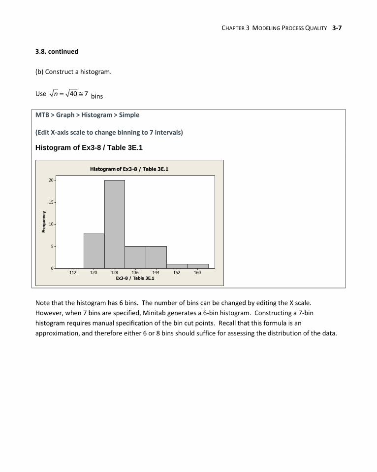
(b) Construct a histogram.

Use 40 7n bins

MTB > Graph > Histogram > Simple (Edit X-axis scale to change binning to 7 intervals)

Histogram of Ex3-8 / Table 3E.1

160152144136128120112

20

15

10

5

0

Ex3-8 / Table 3E.1

Fre

qu

en

cy


Note that the histogram has 6 bins. The number of bins can be changed by editing the X scale.

However, when 7 bins are specified, Minitab generates a 6-bin histogram. Constructing a 7-bin

histogram requires manual specification of the bin cut points. Recall that this formula is an

approximation, and therefore either 6 or 8 bins should suffice for assessing the distribution of the data.


3.8. continued

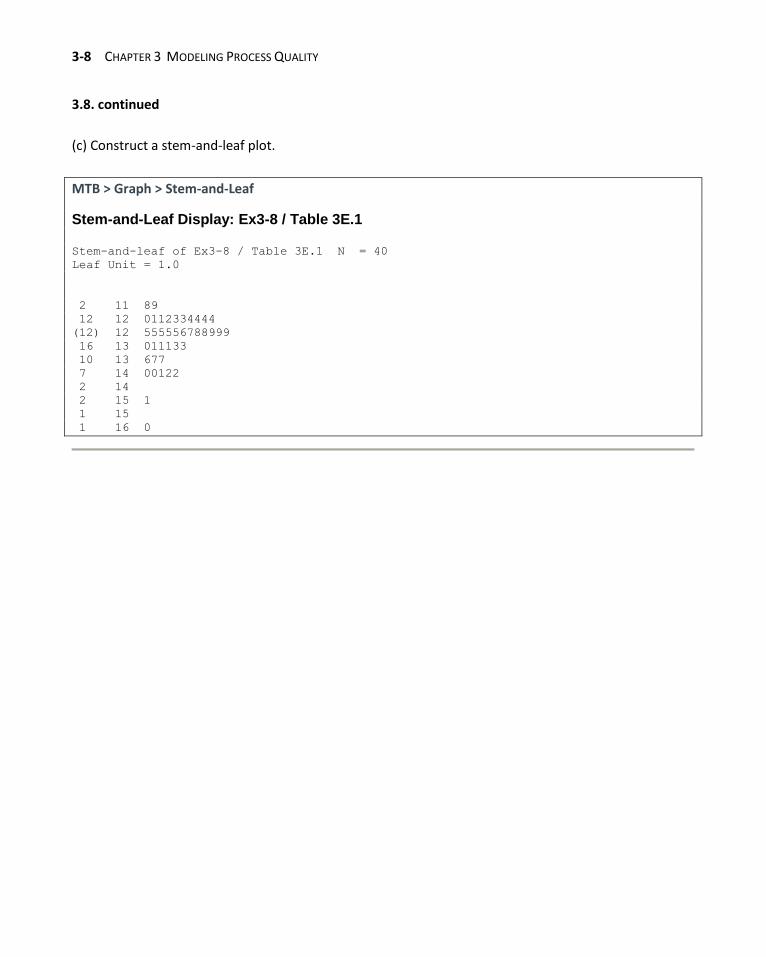
(c) Construct a stem-and-leaf plot.

MTB > Graph > Stem-and-Leaf

Stem-and-Leaf Display: Ex3-8 / Table 3E.1 Stem-and-leaf of Ex3-8 / Table 3E.1 N = 40

Leaf Unit = 1.0

2 11 89

12 12 0112334444

(12) 12 555556788999

16 13 011133

10 13 677

7 14 00122

2 14

2 15 1

1 15

1 16 0


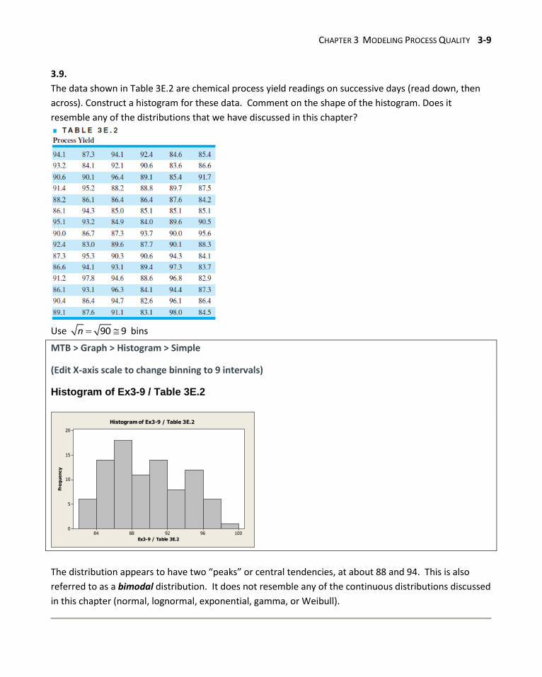
3.9.

The data shown in Table 3E.2 are chemical process yield readings on successive days (read down, then

across). Construct a histogram for these data. Comment on the shape of the histogram. Does it

resemble any of the distributions that we have discussed in this chapter?

Use 90 9n bins

MTB > Graph > Histogram > Simple

(Edit X-axis scale to change binning to 9 intervals)


10096928884

20

15

10

5

0

Ex3-9 / Table 3E.2

Fre

qu

en

cy


The distribution appears to have two “peaks” or central tendencies, at about 88 and 94. This is also

referred to as a bimodal distribution. It does not resemble any of the continuous distributions discussed

in this chapter (normal, lognormal, exponential, gamma, or Weibull).


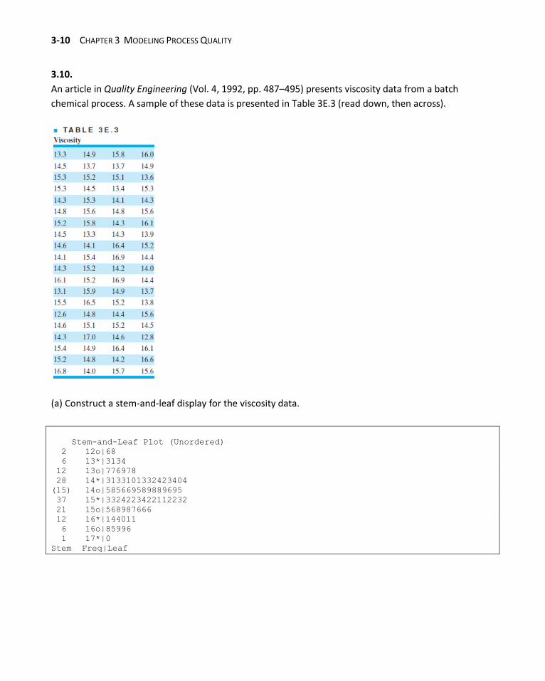
3.10.

An article in Quality Engineering (Vol. 4, 1992, pp. 487–495) presents viscosity data from a batch

chemical process. A sample of these data is presented in Table 3E.3 (read down, then across).

(a) Construct a stem-and-leaf display for the viscosity data.

Stem-and-Leaf Plot (Unordered)

2 12o|68

6 13*|3134

12 13o|776978

28 14*|3133101332423404

(15) 14o|585669589889695

37 15*|3324223422112232

21 15o|568987666

12 16*|144011

6 16o|85996

1 17*|0

Stem Freq|Leaf


3.10. continued

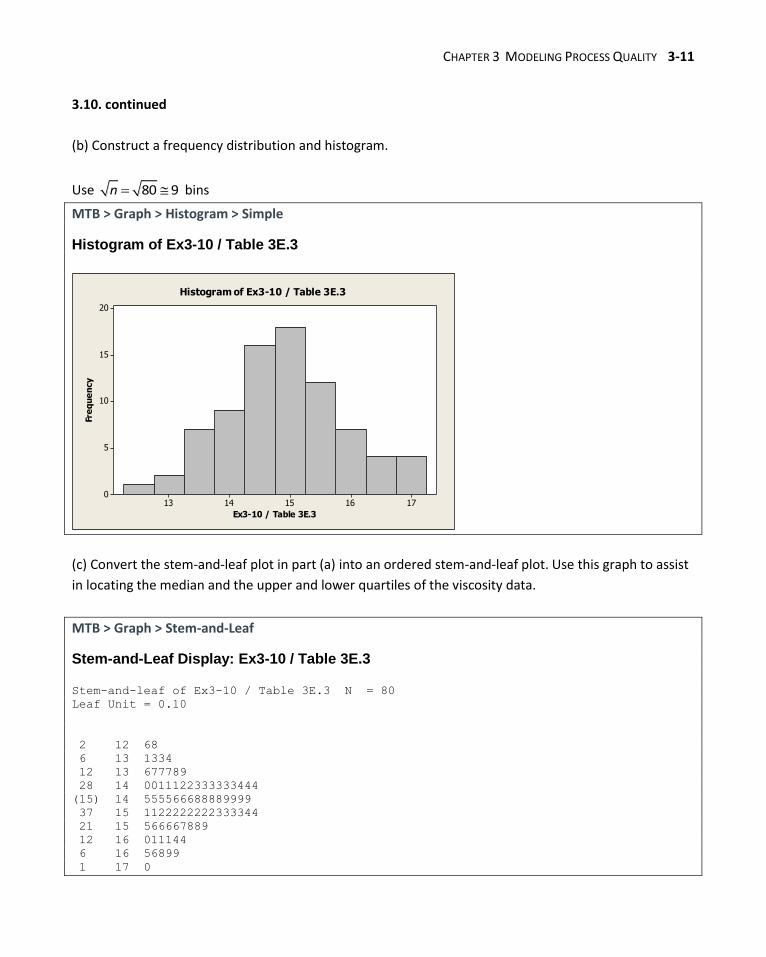
(b) Construct a frequency distribution and histogram.

Use 80 9n bins

MTB > Graph > Histogram > Simple


1716151413

20

15

10

5

0

Ex3-10 / Table 3E.3

Fre

qu

en

cy


(c) Convert the stem-and-leaf plot in part (a) into an ordered stem-and-leaf plot. Use this graph to assist

in locating the median and the upper and lower quartiles of the viscosity data.

MTB > Graph > Stem-and-Leaf

Stem-and-Leaf Display: Ex3-10 / Table 3E.3 Stem-and-leaf of Ex3-10 / Table 3E.3 N = 80

Leaf Unit = 0.10

2 12 68

6 13 1334

12 13 677789

28 14 0011122333333444

(15) 14 555566688889999

37 15 1122222222333344

21 15 566667889

12 16 011144

6 16 56899

1 17 0


3.10.(c) continued

median observation rank is (0.5)(80) + 0.5 = 40.5

x0.50 = (14.9 + 14.9)/2 = 14.9

Q1 observation rank is (0.25)(80) + 0.5 = 20.5

Q1 = (14.3 + 14.3)/2 = 14.3

Q3 observation rank is (0.75)(80) + 0.5 = 60.5

Q3 = (15.6 + 15.5)/2 = 15.55

(d) What are the tenth and ninetieth percentiles of viscosity?

10th percentile observation rank = (0.10)(80) + 0.5 = 8.5

x0.10 = (13.7 + 13.7)/2 = 13.7

90th percentile observation rank is (0.90)(80) + 0.5 = 72.5

x0.90 = (16.4 + 16.1)/2 = 16.25


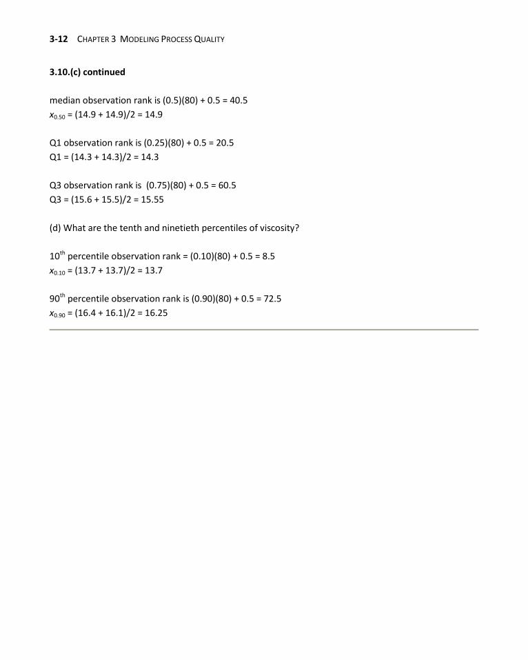
3.11.

Construct and interpret a normal probability plot of the volumes of the liquid detergent bottles in

Exercise 3.1.

MTB > Graph > Probability Plot > Simple and select Normal Distribution

Probability Plot of Ex3-1

16.10016.07516.05016.02516.00015.97515.950

99

95

90

80

70

60

50

40

30

20

10

5

1

Ex3-1

Pe

rce

nt

Mean 16.03

StDev 0.02021

N 12

AD 0.297

P-Value 0.532

Probability Plot of Ex3-1Normal - 95% CI

When plotted on a normal probability plot, the data points tend to fall along a straight line, indicating

that a normal distribution adequately describes the volume of detergent.

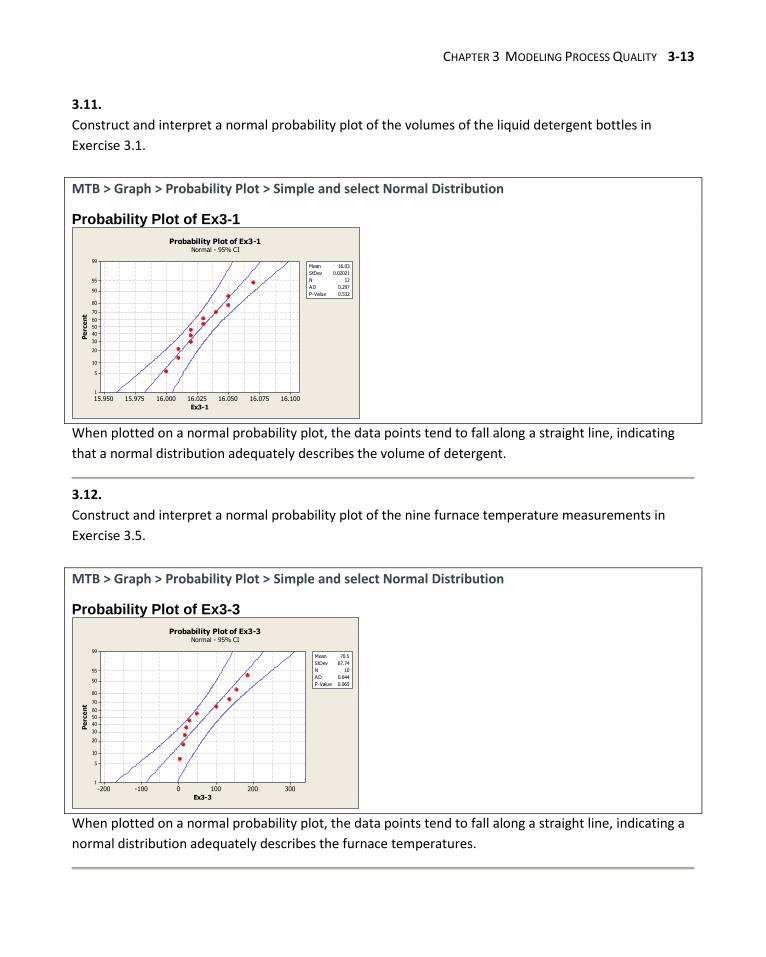
3.12.

Construct and interpret a normal probability plot of the nine furnace temperature measurements in

Exercise 3.5.


Probability Plot of Ex3-3

3002001000-100-200

99

95

90

80

70

60

50

40

30

20

10

5

1

Ex3-3

Pe

rce

nt

Mean 70.5

StDev 67.74

N 10

AD 0.644

P-Value 0.065

Probability Plot of Ex3-3Normal - 95% CI

When plotted on a normal probability plot, the data points tend to fall along a straight line, indicating a

normal distribution adequately describes the furnace temperatures.


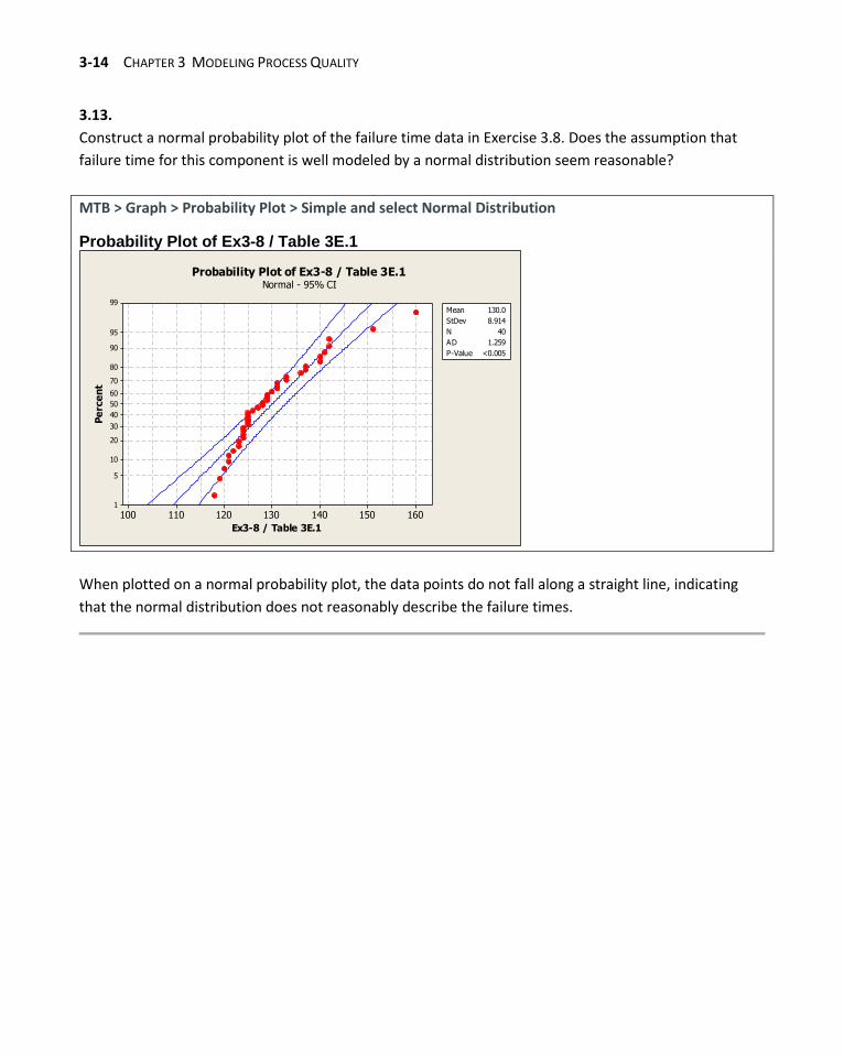
3.13.

Construct a normal probability plot of the failure time data in Exercise 3.8. Does the assumption that

failure time for this component is well modeled by a normal distribution seem reasonable?


Probability Plot of Ex3-8 / Table 3E.1

160150140130120110100

99

95

90

80

70

60

50

40

30

20

10

5

1

Ex3-8 / Table 3E.1

Pe

rce

nt

Mean 130.0

StDev 8.914

N 40

AD 1.259

P-Value <0.005

Probability Plot of Ex3-8 / Table 3E.1Normal - 95% CI

When plotted on a normal probability plot, the data points do not fall along a straight line, indicating

that the normal distribution does not reasonably describe the failure times.

Download - Chapter 1 Quality Improvement in the Modern Business ... Manual for Introduction to Statistical Quality... · Armand V. Feigenbaum 6. Discuss total quality management, the Malcolm

Top Related