Chapter 3Parallel Search
3.1 Search Queries3.2 Data Partitioning3.3 Search Algorithms3.4 Summary3.5 Bibliographical Notes3.6 Exercises
3.1. Search Queries
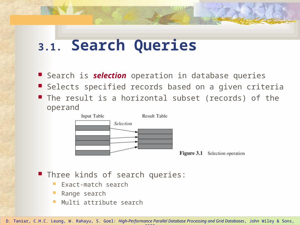
Search is selection operation in database queries Selects specified records based on a given criteria The result is a horizontal subset (records) of the operand
Three kinds of search queries: Exact-match search Range search Multi attribute search
D. Taniar, C.H.C. Leung, W. Rahayu, S. Goel: High-Performance Parallel Database Processing and Grid Databases, John Wiley & Sons, 2008
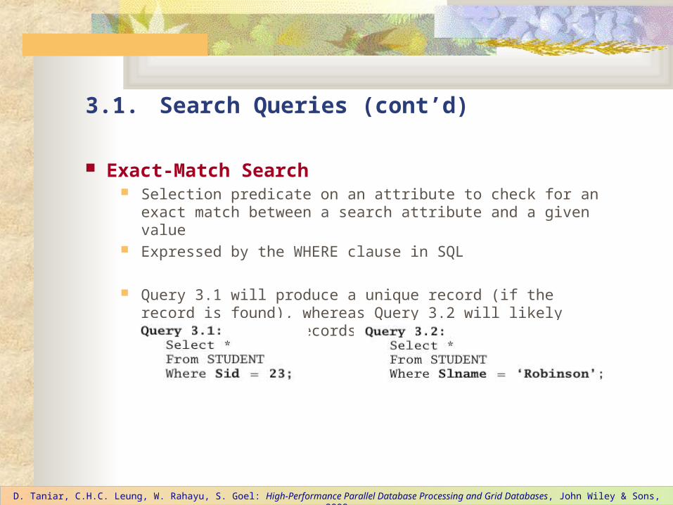
Exact-Match Search Selection predicate on an attribute to check for an exact match
between a search attribute and a given value Expressed by the WHERE clause in SQL
Query 3.1 will produce a unique record (if the record is found), whereas Query 3.2 will likely produce multiple records
3.1. Search Queries (cont’d)
D. Taniar, C.H.C. Leung, W. Rahayu, S. Goel: High-Performance Parallel Database Processing and Grid Databases, John Wiley & Sons, 2008

Range Search Query The search covers a certain range Continuous range search query
Discrete range search query
3.1. Search Queries (cont’d)
D. Taniar, C.H.C. Leung, W. Rahayu, S. Goel: High-Performance Parallel Database Processing and Grid Databases, John Wiley & Sons, 2008

Multiattribute Search Query More than attribute is involved in the search Conjunctive (AND) or Disjunctive (OR) If both are used, it must be in a form of conjunctive prenex normal form
(CPNF)
3.1. Search Queries (cont’d)
D. Taniar, C.H.C. Leung, W. Rahayu, S. Goel: High-Performance Parallel Database Processing and Grid Databases, John Wiley & Sons, 2008

3.2. Data Partitioning
Distributes data over a number of processing elements Each processing element is then executed simultaneously with
other processing elements, thereby creating parallelism Can be physical or logical data partitioning In a shared-nothing architecture, data is placed permanently
over several disks In a shared-everything (shared-memory and shared-disk)
architecture, data is assigned logically to each processor Two kinds of data partitioning:
Basic data partitioning Complex data partitioning
D. Taniar, C.H.C. Leung, W. Rahayu, S. Goel: High-Performance Parallel Database Processing and Grid Databases, John Wiley & Sons, 2008

Basic Data Partitioning Vertical vs. Horizontal data partitioning Vertical partitioning partitions the data vertically across all processors.
Each processor has a full number of records of a particular table. This model is more common in distributed database systems
Horizontal partitioning is a model in which each processor holds a partial number of complete records of a particular table. It is more common in parallel relational database systems
3.2. Data Partitioning (cont’d)
D. Taniar, C.H.C. Leung, W. Rahayu, S. Goel: High-Performance Parallel Database Processing and Grid Databases, John Wiley & Sons, 2008

Basic Data Partitioning Round-robin data partitioning Hash data partitioning Range data partitioning Random-unequal data partitioning
3.2. Data Partitioning (cont’d)
D. Taniar, C.H.C. Leung, W. Rahayu, S. Goel: High-Performance Parallel Database Processing and Grid Databases, John Wiley & Sons, 2008

Round-robin data partitioning Each record in turn is allocated to a processing element in a clockwise
manner “Equal partitioning” or “Random-equal partitioning” Data evenly distributed, hence supports load balance But data is not grouped semantically
3.2. Data Partitioning (cont’d)
D. Taniar, C.H.C. Leung, W. Rahayu, S. Goel: High-Performance Parallel Database Processing and Grid Databases, John Wiley & Sons, 2008
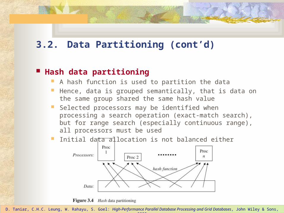
Hash data partitioning A hash function is used to partition the data Hence, data is grouped semantically, that is data on the same group
shared the same hash value Selected processors may be identified when processing a search
operation (exact-match search), but for range search (especially continuous range), all processors must be used
Initial data allocation is not balanced either
3.2. Data Partitioning (cont’d)
D. Taniar, C.H.C. Leung, W. Rahayu, S. Goel: High-Performance Parallel Database Processing and Grid Databases, John Wiley & Sons, 2008

Range data partitioning Spreads the records based on a given range of the partitioning
attribute Processing records on a specific range can be directed to certain
processors only Initial data allocation is skewed too
3.2. Data Partitioning (cont’d)
D. Taniar, C.H.C. Leung, W. Rahayu, S. Goel: High-Performance Parallel Database Processing and Grid Databases, John Wiley & Sons, 2008

Random-unequal data partitioning Partitioning is not based on the same attribute as the retrieval
processing is based on a nonretrieval processing attribute, or the partitioning method is unknown
The size of each partitioning is likely to be unequal Records within each partition are not grouped semantically This is common especially when the operation is actually an operation
based on temporary results obtained from the previous operations
3.2. Data Partitioning (cont’d)
D. Taniar, C.H.C. Leung, W. Rahayu, S. Goel: High-Performance Parallel Database Processing and Grid Databases, John Wiley & Sons, 2008

Basic Data Partitioning Attribute-based data partitioning Non-attribute-based data partitioning
3.2. Data Partitioning (cont’d)
D. Taniar, C.H.C. Leung, W. Rahayu, S. Goel: High-Performance Parallel Database Processing and Grid Databases, John Wiley & Sons, 2008

Complex Data Partitioning Basic data partitioning is based on a single attribute (or no attribute) Complex data partitioning is based on multiple attributes or is based
on a single attribute but with multiple partitioning methods
Hybrid-Range Partitioning Strategy (HRPS) Multiattribute Grid Declustering (MAGIC) Bubba’s Extended Range Declustering (BERB)
3.2. Data Partitioning (cont’d)
D. Taniar, C.H.C. Leung, W. Rahayu, S. Goel: High-Performance Parallel Database Processing and Grid Databases, John Wiley & Sons, 2008
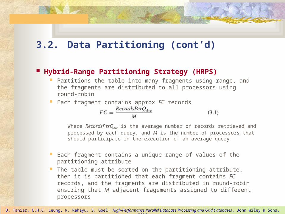
Hybrid-Range Partitioning Strategy (HRPS) Partitions the table into many fragments using range, and the
fragments are distributed to all processors using round-robin Each fragment contains approx FC records
Where RecordsPerQAve is the average number of records retrieved and processed by each query, and M is the number of processors that should participate in the execution of an average query
Each fragment contains a unique range of values of the partitioning attribute
The table must be sorted on the partitioning attribute, then it is partitioned that each fragment contains FC records, and the fragments are distributed in round-robin ensuring that M adjacent fragements assigned to different processors
3.2. Data Partitioning (cont’d)
D. Taniar, C.H.C. Leung, W. Rahayu, S. Goel: High-Performance Parallel Database Processing and Grid Databases, John Wiley & Sons, 2008

Hybrid-Range Partitioning Strategy (HRPS) Example: 10000 student records, and the partitioning attribute is
StudentID (PK) that ranges from 1 to 10000. Assume the average query retrieves a range of 500 records (RecordsPerQ=500). Queries access students per year enrolment wth average results of 500 records. Assume the optimal performance is achieved when 5 processors are used (M=5)
The table will be partitioned into 100 fragments Three cases: M = N, M > N, or M < N (where N is the number of
processors in the configuration, and M is the number of processors participating in the query execution
3.2. Data Partitioning (cont’d)
D. Taniar, C.H.C. Leung, W. Rahayu, S. Goel: High-Performance Parallel Database Processing and Grid Databases, John Wiley & Sons, 2008

Hybrid-Range Partitioning Strategy (HRPS) Case 1: M = N Because the query will overlap with 5-6 fragments, all processors will
be used (high degree of parallelism) Compared with hash partitioning: Hash will also use N processors,
since it cannot localize the execution of a range query Compared with range partitioning: Range will only use 1-2 processors,
and hence the degree of parallelism is small
3.2. Data Partitioning (cont’d)
D. Taniar, C.H.C. Leung, W. Rahayu, S. Goel: High-Performance Parallel Database Processing and Grid Databases, John Wiley & Sons, 2008
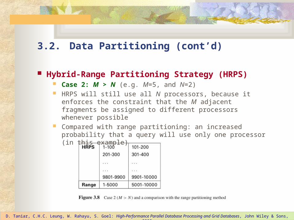
Hybrid-Range Partitioning Strategy (HRPS) Case 2: M > N (e.g. M=5, and N=2) HRPS will still use all N processors, because it enforces the constraint
that the M adjacent fragments be assigned to different processors whenever possible
Compared with range partitioning: an increased probability that a query will use only one processor (in this example)
3.2. Data Partitioning (cont’d)
D. Taniar, C.H.C. Leung, W. Rahayu, S. Goel: High-Performance Parallel Database Processing and Grid Databases, John Wiley & Sons, 2008
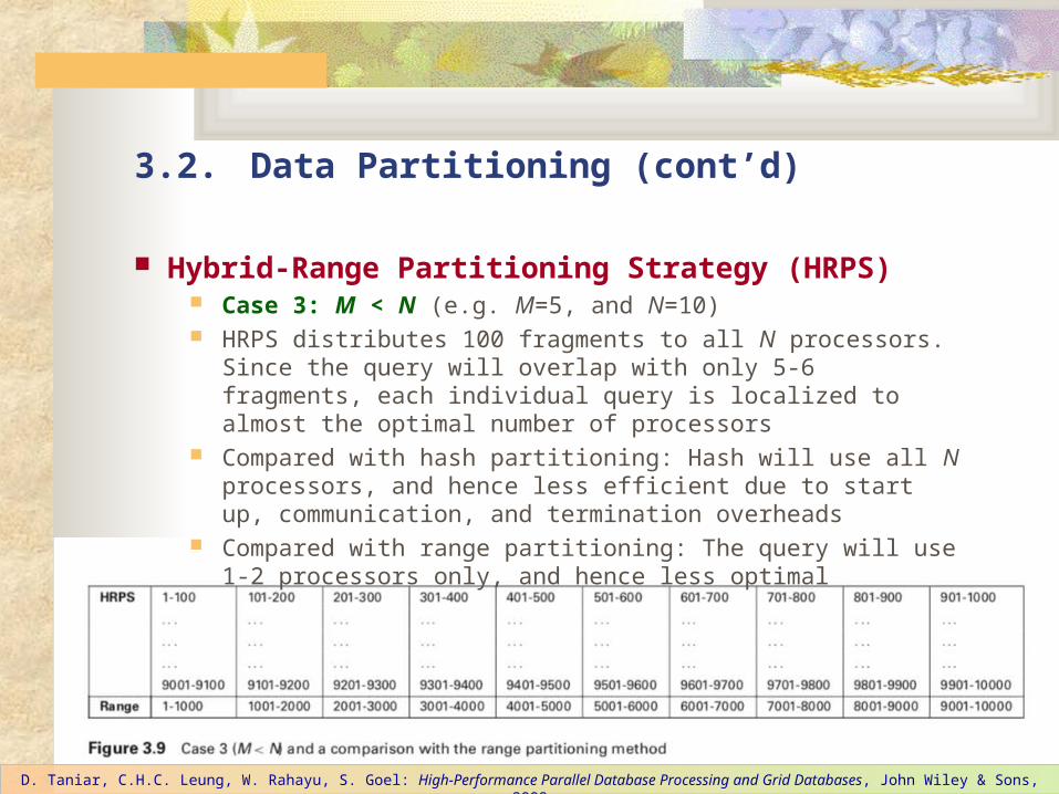
Hybrid-Range Partitioning Strategy (HRPS) Case 3: M < N (e.g. M=5, and N=10) HRPS distributes 100 fragments to all N processors. Since the query
will overlap with only 5-6 fragments, each individual query is localized to almost the optimal number of processors
Compared with hash partitioning: Hash will use all N processors, and hence less efficient due to start up, communication, and termination overheads
Compared with range partitioning: The query will use 1-2 processors only, and hence less optimal
3.2. Data Partitioning (cont’d)
D. Taniar, C.H.C. Leung, W. Rahayu, S. Goel: High-Performance Parallel Database Processing and Grid Databases, John Wiley & Sons, 2008

Hybrid-Range Partitioning Strategy (HRPS) Support for Small Tables
If the number of fragments of a table is less than the number of processors, then the table will automatically be partitioned across a subset of the processors
Support for Tables with Nonuniform Distributions of the Partitioning Attribute Values
Because the cardinality of each fragment is not based on the value of the partitioning attribute value, once the HRPS determines the cardinality of each fragment, it will partition a table based on that value
3.2. Data Partitioning (cont’d)
D. Taniar, C.H.C. Leung, W. Rahayu, S. Goel: High-Performance Parallel Database Processing and Grid Databases, John Wiley & Sons, 2008

Multiattribute Grid Declustering (MAGIC) Based on multiple attributes - to support search queries based on
either of data partitioning attributes Support range and exact match search on each of the partitioning
attributes Example: Query 1 (one-half of the accesses) Slname=‘Roberts’, and
Query 2 (the other half) SID between 98555 and 98600. Assume both queries produce only a few records
Create a two-dim grid with the two partitioning attributes (Slname and SID). The number of cells in the grid equal the number of processing elements
Determine the range value for each column and row, and allocate a processor in each cell in the grid
3.2. Data Partitioning (cont’d)
D. Taniar, C.H.C. Leung, W. Rahayu, S. Goel: High-Performance Parallel Database Processing and Grid Databases, John Wiley & Sons, 2008

Multiattribute Grid Declustering (MAGIC) Query 1 (exact match on Slname): Hash partitioning can localize the
query processing on one processor. MAGIC will use 6 processors Query 2 (range on SID): if the hash partitioning uses Slname, whereas
the query is on SID, the query must use all 36 processors. MAGIC on the other hand, will only use 6 processors.
Compared with range partitioning, suppose the partitioning is based on SID, then Q1 will use 36 processors whilst Q2 will use 1 processor
3.2. Data Partitioning (cont’d)
D. Taniar, C.H.C. Leung, W. Rahayu, S. Goel: High-Performance Parallel Database Processing and Grid Databases, John Wiley & Sons, 2008

Bubba’s Extended Range Declustering (BERB) Another multiattribute partitioning method - used in the Bubba
Database Machine Two levels of data partitioning: primary and secondary data
partitioning Step 1: Partition the table based on the primary partitioning attribute
and uses a range partitioning method
3.2. Data Partitioning (cont’d)
D. Taniar, C.H.C. Leung, W. Rahayu, S. Goel: High-Performance Parallel Database Processing and Grid Databases, John Wiley & Sons, 2008

Bubba’s Extended Range Declustering (BERB) Step 2: Each fragment is scanned and an ‘aux’ table is created from
the attribute value of the secondary partitioning attribute and a list of processors containing the original records
Table 3.4 shows the ‘aux’ table (called Table IndexB)
3.2. Data Partitioning (cont’d)
D. Taniar, C.H.C. Leung, W. Rahayu, S. Goel: High-Performance Parallel Database Processing and Grid Databases, John Wiley & Sons, 2008

Bubba’s Extended Range Declustering (BERB) Step 3: The ‘aux’ table is range partitioned on the secondary
partitioning attribute (e.g. Slname) Step 4: Place the fragments from steps 1 and 3 into multiple
processors
3.2. Data Partitioning (cont’d)
D. Taniar, C.H.C. Leung, W. Rahayu, S. Goel: High-Performance Parallel Database Processing and Grid Databases, John Wiley & Sons, 2008

3.3. Search Algorithms
Serial search algorithms: Linear search Binary search
Parallel search algorithms: Processor activation or involvement Local searching method Key comparison
D. Taniar, C.H.C. Leung, W. Rahayu, S. Goel: High-Performance Parallel Database Processing and Grid Databases, John Wiley & Sons, 2008

Linear Search Exhaustive search - search each record one by one until it is found or
end of table is reached
Scanning cost: 1/2 x R / P x IO Select cost: 1/2 x |R| x (tr + tw) Comparison cost: 1/2 x |R| x tr Result generation cost: x |R| x tw, where is the search query
selection ratio Disk writing cost: x R / P x IO
3.3. Search Algorithms (cont’d)
D. Taniar, C.H.C. Leung, W. Rahayu, S. Goel: High-Performance Parallel Database Processing and Grid Databases, John Wiley & Sons, 2008

Binary Search Must be pre-sorted The complexity is O(log2(n)) The cost components for binary search are similar to those of linear
search, except that the component of 1/2 in linear search is now replaced with log2:
3.3. Search Algorithms (cont’d)
D. Taniar, C.H.C. Leung, W. Rahayu, S. Goel: High-Performance Parallel Database Processing and Grid Databases, John Wiley & Sons, 2008
Parallel search algorithms: Processor activation or involvement Local searching method Key comparison
D. Taniar, C.H.C. Leung, W. Rahayu, S. Goel: High-Performance Parallel Database Processing and Grid Databases, John Wiley & Sons, 2008
3.3. Search Algorithms (cont’d)
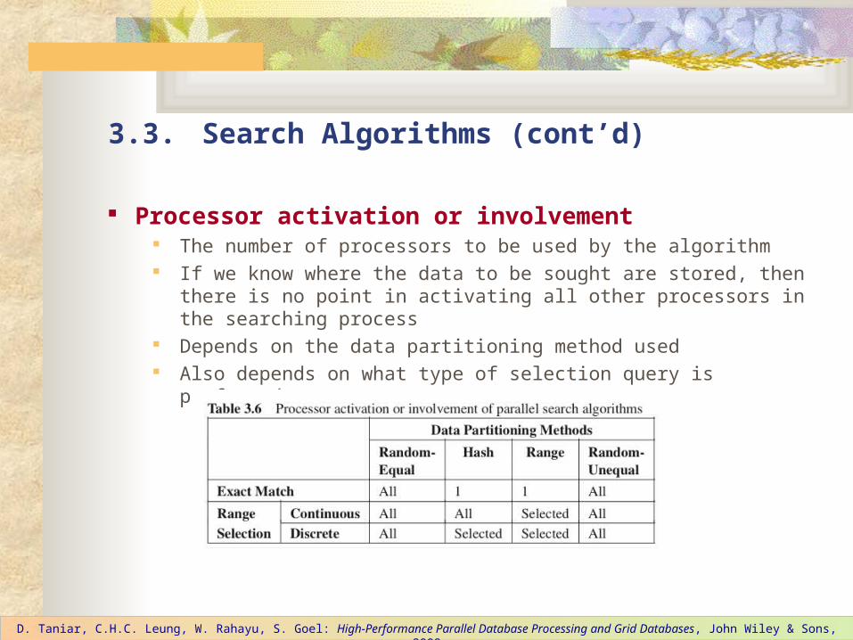
Processor activation or involvement The number of processors to be used by the algorithm If we know where the data to be sought are stored, then there is no point in
activating all other processors in the searching process Depends on the data partitioning method used Also depends on what type of selection query is performed
D. Taniar, C.H.C. Leung, W. Rahayu, S. Goel: High-Performance Parallel Database Processing and Grid Databases, John Wiley & Sons, 2008
3.3. Search Algorithms (cont’d)

Local searching method The searching method applied to the processor(s) involved in the searching
process Depends on the data ordering, regarding the type of the search (exact
match of range)
D. Taniar, C.H.C. Leung, W. Rahayu, S. Goel: High-Performance Parallel Database Processing and Grid Databases, John Wiley & Sons, 2008
3.3. Search Algorithms (cont’d)

Key comparison Compares the data from the table with the condition specified by the query When a match is found: continue to find other matches, or terminate Depends on whether the data in the table is unique or not
D. Taniar, C.H.C. Leung, W. Rahayu, S. Goel: High-Performance Parallel Database Processing and Grid Databases, John Wiley & Sons, 2008
3.3. Search Algorithms (cont’d)
3.4. Summary
Search queries in SQL using the WHERE clause
Search predicates indicates the type of search operation Exact-match, range (continuous or discrete), or multiattribute search
Data partitioning is a basic mechanism of parallel search Single attribute-based, no attribute-based, or multiattribute-based
partitioning
Parallel search algorithms have three main components Processor involvement, local searching method, and key comparison
D. Taniar, C.H.C. Leung, W. Rahayu, S. Goel: High-Performance Parallel Database Processing and Grid Databases, John Wiley & Sons, 2008

Continue to Chapter 4…


