
Chapter 7 - Local Stabilization 1
Chapter 7 – Local
Stabilization
Self-StabilizationShlomi DolevMIT Press , 2000
Draft of January 2004Shlomi Dolev, All Rights Reserved ©

Chapter 7 - Local Stabilization 2
Chapter 7: roadmap
7.1 Superstabilization 7.2 Self-Stabilizing Fault-Containing
Algorithms7.3 Error-Detection Codes and Repair

Chapter 7 - Local Stabilization 3
Dynamic System
Algorithms for dynamic systems are designed to cope with failures of processors with no global re-initialization.
Such algorithms consider only global states reachable from a predefined initial state under a restrictive sequence of failures and attempt to cope with such failures with as few adjustments as possible.
Self Stabilization
Self-stabilizing algorithms are designed to guarantee a particular behavior finally.
Traditionally, changes in the communications graph were ignored.
Dynamic System & Self Stabilization
Superstabilizing algorithms combine the benefits of both self-stabilizing and dynamic algorithms

Chapter 7 - Local Stabilization 4
Definitions
A Superstabilizing Algorithm:
Must be self-stabilizing Must preserve a “passage predicate” Should exhibit fast convergence rate
Passage Predicate - Defined with respect to a class of topology changes(A topology change falsifies legitimacy and therefore the passage predicate must be weaker than legitimacy but strong enough to be
useful).
Chapter 7 - Local Stabilization 5
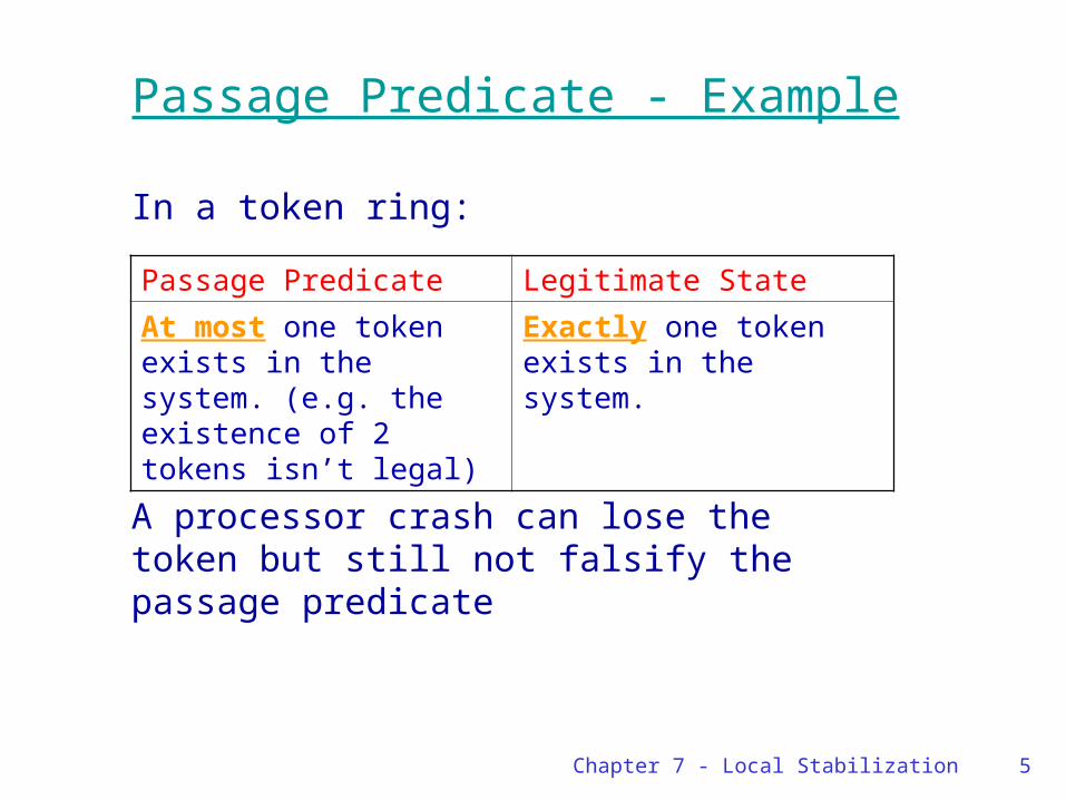
Passage Predicate - Example
In a token ring:
A processor crash can lose the token but still not falsify the passage predicate
Passage Predicate Legitimate State
At most one token exists in the system. (e.g. the existence of 2 tokens isn’t legal)
Exactly one token exists in the system.

Chapter 7 - Local Stabilization 6
Evaluation of a Super-Stabilizing Algorithm
a. Time complexityThe maximal number of rounds that have passed from a legitimate state through a single topology change and ends in a legitimate state
b. Adjustment measureThe maximal number of processors that must change their local state upon a topology change, in order to achieve legitimacy

Chapter 7 - Local Stabilization 7
Motivation for Super-Stabilization
A self-stabilizing algorithm that does not ignore theoccurrence of topology changes (“events”) will beinitialized in a predefined way and react better to dynamic changes during execution
Question:Is it possible, for the algorithm that detects a fault, when it occurs, to maintain a “nearly legitimate” state during convergence?

Chapter 7 - Local Stabilization 8
Motivation for Super-Stabilization
While transient faults are rare (but harmful), a dynamic change in the topology may be frequent.
Thus, a super-stabilizing algorithm has a lower worst-case time measure for reaching a legitimate state again, once a topology change occurs.
In the following slides we present a self-stabilizing and a super-stabilizing algorithm for the graph coloring task.

Chapter 7 - Local Stabilization 9
Graph Coloring
a. The coloring task is to assign a color value to each processor, such that no two neighboring processors are assigned the same color.
b. Minimization of the colors number is not required. The algorithm uses Δ+1 colors, where Δ is an upper bound on a processor’s number of neighbors.
c. For example:

Chapter 7 - Local Stabilization 10
If Pi has the color of one of its neighbors with a higher ID, it chooses another color and writes it.
Graph Coloring - A Self-Stabilzing Algorithm
01 Do forever02 GColors := 003 For m:=1 to δ do04 lrm:=read(rm)
05 If ID(m)>i then 06 GColors := GColors U lrm.color
07 od08 If colori GColors then
09 colori:=choose(\\ GColors)
10 Write ri.color := color
11 od
Colors of Pi’s
neighbors
Gather only thecolors of neighborswith greater ID than Pi’s.

Chapter 7 - Local Stabilization 11
Id = 3 Id = 1
Id = 5
Id = 4 Id = 2
Graph Coloring - Self-Stabilzing Algorithm - Simulation
GColors = { Blue }
GColors = { Blue }
GColors = { Blue }
GColors = { Blue }
GColors = {}
Phase I

Chapter 7 - Local Stabilization 12
Id = 3 Id = 1
Id = 5
Id = 4 Id = 2
GColors = { Green }
GColors = {}
GColors = {}
GColors = { Blue , green , Red }
GColors = { Blue , green }
Phase II
Graph Coloring - Self-Stabilzing Algorithm - Simulation

Chapter 7 - Local Stabilization 13
Id = 3 Id = 1
Id = 5
Id = 4 Id = 2
Stabilized
GColors = { Green }
GColors = {}
GColors = {}
GColors = { Blue , green , Red }
GColors = { Blue , green }
Phase III
Graph Coloring - Self-Stabilzing Algorithm - Simulation

Chapter 7 - Local Stabilization 14
Graph Coloring - Self-Stabilizing Algorithm (continued)
What happens when a change in the topology occurs ?
If a new neighbor is added, it is possible that twoprocessors have the same color. It is possible that during convergence every processor will change its color.Example:
1 2 3 4 5
i=4GColo
rs
{blue}
i=5GColo
rs
ø
i=1GColo
rs
{blue}
i=2GColo
rs
{red}
i=3GColo
rs
{red}
i=2GColo
rs
{blue}
i=1GColo
rs
{red}
Stabilized
But in what cost ?

Chapter 7 - Local Stabilization 15
Graph Coloring – Super-Stabilizing Motivation
a. Every processor changed its color but only one processor really needed to.
b. If we could identify the topology change we could maintain the changes in its environment.
c. We’ll add some elements to the algorithm:a. AColor – A variable that collects all of the
processor neighbors’ colors.b. Interrupt section – Identify the problematic area.c. - A symbol to flag a non-existing color.

Chapter 7 - Local Stabilization 16
01 Do forever02 AColors := 03 GColors := 04 For m:=1 to δ do05 lrm:=read(rm)
06 AColors := AColors U lrm.color07 If ID(m)>i then GColors := GColors U
lrm.color08 od
09 If colori = ┴ or colori GColors then
10 colori:=choose(\\ AColors)
11 Write ri.color := color12 od13 Interrupt section14 If recoverij and j > i then
15 Colori := ┴16 Write ri.color := ┴
All of Pi neighbors’
colors
Graph Coloring – A Super-Stabilizing Algorithm
Activated after a topology change toidentify the critical processor
recoveri,j is the interrupt which Pi gets upon a
change in the communication between Pi and Pj

Chapter 7 - Local Stabilization 17
Graph Coloring - Super-Stabilizing Algorithm - Example
Notice that the new algorithm stabilizes faster
than the previous one.Let us consider the previous example, this
time using the super-stabilizing algorithm:
1 2 3 4 5
i=4GColors = {blue}AColors =
{blue,red}
Stabilized
In O(1).
Color4 =
r4.color =

Chapter 7 - Local Stabilization 18
Graph Coloring – Super-Stabilizing Proof
Lemma 1: This algorithm is self-stabilizing.Proof by induction:a. After the first iteration:
a. The value doesn’t exist in the system.b. Pn has a fixed value.
b. Assume that Pk has a fixed value i<k<n.
If Pi has a Pk neighbor then Pi does not
change to Pk’s color, but chooses a different
color.Due to the assumptions we get that Pi’s color
becomes fixed for 1≤i≤n, so the system stabilizes.

Chapter 7 - Local Stabilization 19
Graph Coloring – Super-Stabilizing
Passage Predicate – The color of a neighboring processor is always different in everyexecution that starts in a safe configuration,in which only a single topology change occursbefore the next safe configuration is reached
Chapter 7 - Local Stabilization 20
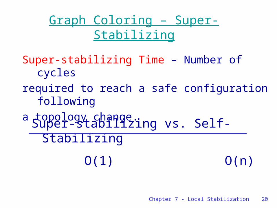
Graph Coloring – Super-Stabilizing
Super-stabilizing Time – Number of cycles required to reach a safe configuration
following a topology change.
Super-stabilizing vs. Self-Stabilizing
O(1) O(n)

Chapter 7 - Local Stabilization 21
Graph Coloring – Super-Stabilizing
Adjustment Measure – The number of processors that changes color upon a topology change.The super-stabilizing algorithm changes one processor color, the one which had the singletopology change

Chapter 7 - Local Stabilization 22
Chapter 7: roadmap
7.1 Superstabilization 7.2 Self-Stabilizing Fault-Containing
Algorithms7.3 Error-Detection Codes and Repair

Chapter 7 - Local Stabilization 23
Self-Stabilizing Fault-Containing Algorithms
Fault model : Several transient faults in the system.This fault model is less severe than dynamic changes faults, and considers the case where f transient faults occurred, changing the state of f processors.
The goal of self-stabilizing fault containing algorithms :a) From any arbitrary configuration, a safe
configuration is reached.b) Starting from a safe configuration followed by
transient faults that corrupt the state of f processors, a safe configuration is reached within O(f) cycles.

Chapter 7 - Local Stabilization 24
A Self-Stabilizing Algorithm for Fixed Output Tasks
Our Goal: to design a self-stabilizing fault-containing algorithm for fixed-output fixed-input tasks.
Fixed Input: the algorithm has a fixed input (like its fixed local topology), Ii will contain the input for processor Pi
Fixed Output: the variable Oi will contain the output of processor Pi, the output should not change over time.
A version of the update algorithm is a self stabilizing algorithm for any fixed-input fixed-output task.

Chapter 7 - Local Stabilization 25
Fixed-output algorithm for Processor Pi
1. upon a pulse2. ReadSeti := Ø
3. forall Pj N(i) do
4. ReadSeti := ReadSeti read(Processorsj)
5. ReadSeti := ReadSeti \\ <i,*,*>
6. ReadSeti := ReadSeti ++ <*,1,*>
7. ReadSeti := ReadSeti {<i,0,Ii>}
8. forall Pj processors(ReadSeti) do
9. ReadSeti := ReadSeti \\ NotMinDist(Pj, ReadSeti)
10. write Processorsi := ConPrefix(ReadSeti)
11. write Oi := ComputeOutput(Inputs(Processorsi))

Chapter 7 - Local Stabilization 26
Explaining the Algorithm
The algorithm is a version of the self-stabilizing update algorithm, it has an extra Ii variable in each <id, dis, Ii> tuple which contains the fixed input of the processor Pi
Just like in the update algorithm, it is guaranteed that eventually each processor will have a tuple for all other processors
Each processor will have all the inputs and will compute the correct output.
But is this algorithm fault containing?

Chapter 7 - Local Stabilization 27
Does this Algorithm have the Fault-containment Property?
Error Scenario (assuming output is OR of inputs): In a safe configuration P5 has a tuple <1,4,0> A fault has occurred and changed it to <1,1,1> Error propagation :
Conclusion : It doesn’t have this property. The system stabilizes only after O(d/2) cycles
cycle : 0
P1 P2 P3 P4 P5
I=0
I=0
I=0
I=0
I=0
O1=0
O2=0
O3=0
O4=0 O5=0<1,1,0> <1,2,0> <1,4,0><1,3,0>1
O4=0
<1,1,1><1,3,0>
O5=12 <1,2,1>
O4=1 <1,4,0>
O5=0
3 <1,3,1>
O4=0
<1,3,0>
O5=1
4
O5=0<1,4,0>

Chapter 7 - Local Stabilization 28
Fault Containment – Naive Approach
A processor that is about to change its output waits for d cycles before it does so
This approach ensures : Stabilization from every arbitrary state Starting in a safe configuration followed by
several simultaneous transient faults, only the output of the processors that experienced a fault can be changed and each such change is a change to correct output value.
During this interval correct input values propagate towards the faulty processor

Chapter 7 - Local Stabilization 29
Fault Containment – Naive Approach (cont.)
The above approach ensures self-stabilization, but has a serious drawback : The time it takes for the correct input values
to propagate to the faulty processors and correct its output is O(d), which contradicts the second requirement of self stabilizing fault-containment
This requirement states that a safe configuration is reached within O(f) cycles
Lets consider a more sophisticated approach to meet all fault-containment requirements

Chapter 7 - Local Stabilization 30
Designing a Fault-containing Algorithm
Evidence : The values of all the Ii fields in Processorsi. Each tuple will contain evidence in addition to its other 3 fields
The additional Ai variable enables the processors that experienced a fault to learn quickly about the inputs of the remote processors
When a processor experiences a fault, the Ai variables of most of the processors within distance 2f+1 or less from it are the set of correct inputs
We should maintain this as an invariant throughout the algorithm for a time sufficient to let the faulty processors regain the correct input values Ii of the other processors

Chapter 7 - Local Stabilization 31
Self-stabilizing Fault-containing Algorithm for Processor Pi
1. upon a pulse2. ReadSeti := Ø3. forall Pj N(i) do4. ReadSeti := ReadSeti read(Processorsj)5. if (RepairCounteri ≠ d + 1) then //in repair process6. RepairCounteri := min(RepairCounteri,
read(RepairCounterj))7. od8. ReadSeti := ReadSeti \\ <i,*,*,*>9. ReadSeti := ReadSeti ++ <*,1,*,*>10. ReadSeti := ReadSeti <i,0,Ii,Ai>11. forall Pj processors(ReadSeti) do12. ReadSeti := ReadSeti \\ NotMinDist(Pj, ReadSeti)13. write Processorsi := ConPrefix(ReadSeti)

Chapter 7 - Local Stabilization 32
Self-stabilizing Fault-containing Algorithm – (cont.)
14. if (RepairCounteri = d + 1) then //not in repair process
15. if (Oi ≠ ComputeOutputi(Inputs(Processorsi))) or
16. (<*,*,*,A> Processorsi | A ≠ Inputs(Processorsi))
17. then RepairCounteri := 0 //repair started
18. else //in repair process19. RepairCounteri := min(RepairCounteri + 1, d + 1)
20. write Oi := ComputeOutputi(RepairCounteri,
21. MajorityInputs(Processorsi))
22. if (RepairCounteri = d + 1) then //repair over
23. Ai := Inputs(Processorsi)

Chapter 7 - Local Stabilization 33
Explaining the Algorithm
Initial state: RepairCounteri = d + 1. A change in the RepairCounteri variable occurs when Pi detects an error in its state, or when an error from another processor propagates towards it during the repair process
ComputeOutput is applied on the majority of inputs of processors with distance ≤ RepairCounteri from Pi, thus assuring that eventually the distance 2f+1 is reached and that Oi is set correcly
The value of Ai doesn’t change throughout the repair process, thus maintaining the invariant needed for the faulty processors to regain the correct input values and eventually present a correct output

Chapter 7 - Local Stabilization 34
cycle :
P1 P2 P3 P4 P5
I=0
I=0
I=0
I=0
I=0
O=0 O=0 O=0 O=0 O=0
<1,1,0,A1> <1,2,0,A1>
0
<1,4,0,A1><1,3,0,A1>
P6
I=0
<1,5,0,A1>
A2:i1= 0 A4:i1= 0
A3:i1= 0A4:i1= 0
A5:i1= 0
Error scenario : Input of P1 at (P2 and P4) erroneously alters to 1 Input of P1 at (A2 and A4) evidences erroneously alters to 1 The erroneous input propagates to P3 and so do the
evidences, causing it to calculate erroneous output based on majority inputs at distance ≤ 1
The output is fixed in P3 once the distance grows to ≤ 2.
A2:i1= 0
A1:i1= 0A2:i1= 1 A4:i1= 1
1
<1,1,1,A1> <1,3,1,A1><1,0,0,A1>
A4:i1= 1
<1,1,0,A1>
2
<1,3,0,A1>
A2:i1= 1
<1,2,1,A1>
3
<1,2,0,A1>
O=1
<1,3,1,A1>
4
O=0
<1,3,0,A1>

Chapter 7 - Local Stabilization 35
Error Scenario
Initially the network graph is in a safe configuration
In the first cycle red processors experience several faults : The evidence considering the blue processor
is erroneous. The distance to the blue processor and its
input are also erroneous. In the next cycles the error propagates
throughout the graph The output becomes erroneous at many
processors, but convergence back to the safe state is quick

Chapter 7 - Local Stabilization 36
Feel the Power (example)
…
…
…
Cycle:
01234
Regular
Wrong evidence
Source (blue)
Wrong output
Wrong evidence
and output
(repairCounter)

Chapter 7 - Local Stabilization 37
Algorithm Analysis
Ai of processor Pi stays unchanged for (d+1) cycles since the repair process started, which ensures that the fault factor doesn’t grow
The majority-based output calculation is applied during the repair process After 2f+1 cycles the majority of inputs
around the faulty processor is correct, applying correct output computation
In that manner, after 2f+1 cycles the system’s output stabilizes with correct values, despite the continuing changes in processors’ internal states (for d+1 cycles)

Chapter 7 - Local Stabilization 38
Conclusions
Compared to the naive implementation, this algorithm significantly shortens the system stabilization time
The price we pay for this improvement : Network load grows because each tuple
includes an additional variable Ai of size O(n) (n – number of processors).
During the algorithm execution, faulty output is allowed for non-faulty processors during short periods of time
Chapter 7 - Local Stabilization 39
Chapter 7: roadmap
7.1 Superstabilization 7.2 Self-Stabilizing Fault-Containing
Algorithms7.3 Error-Detection Codes and Repair


