University of Rhode Island University of Rhode Island
DigitalCommons@URI DigitalCommons@URI
Open Access Dissertations
2021
CHARACTERIZATION OF IMPACT PILE DRIVING SIGNALS AND CHARACTERIZATION OF IMPACT PILE DRIVING SIGNALS AND
FIN WHALE VOCALIZATIONS AT THE BLOCK ISLAND WIND FARM FIN WHALE VOCALIZATIONS AT THE BLOCK ISLAND WIND FARM
SITE SITE
Jennifer L. Amaral
Follow this and additional works at: https://digitalcommons.uri.edu/oa_diss
CHARACTERIZATION OF IMPACT PILE DRIVING SIGNALS AND FIN
WHALE VOCALIZATIONS AT THE BLOCK ISLAND WIND FARM SITE
BY
JENNIFER L. AMARAL
A DISSERTATION SUBMITTED IN PARTIAL FULFILLMENT OF THE
REQUIREMENTS FOR THE DEGREE OF
DOCTOR OF PHILOSOPHY
IN
OCEAN ENGINEERING
UNIVERSITY OF RHODE ISLAND
2021

DOCTOR OF PHILOSOPHY DISSERTATION
OF
JENNIFER L. AMARAL
APPROVED:
Dissertation Committee:
Major Professor James H. Miller
Gopu R. Potty
Kathleen Vigness-Raposa
Ying-Tsong Lin
Brenton DeBoef
DEAN OF THE GRADUATE SCHOOL
UNIVERSITY OF RHODE ISLAND
2021
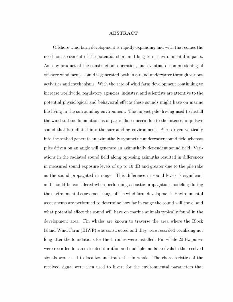
ABSTRACT
Offshore wind farm development is rapidly expanding and with that comes the
need for assessment of the potential short and long term environmental impacts.
As a by-product of the construction, operation, and eventual decommissioning of
offshore wind farms, sound is generated both in air and underwater through various
activities and mechanisms. With the rate of wind farm development continuing to
increase worldwide, regulatory agencies, industry, and scientists are attentive to the
potential physiological and behavioral effects these sounds might have on marine
life living in the surrounding environment. The impact pile driving used to install
the wind turbine foundations is of particular concern due to the intense, impulsive
sound that is radiated into the surrounding environment. Piles driven vertically
into the seabed generate an azimuthally symmetric underwater sound field whereas
piles driven on an angle will generate an azimuthally dependent sound field. Vari-
ations in the radiated sound field along opposing azimuths resulted in differences
in measured sound exposure levels of up to 10 dB and greater due to the pile rake
as the sound propagated in range. This difference in sound levels is significant
and should be considered when performing acoustic propagation modeling during
the environmental assessment stage of the wind farm development. Environmental
assessments are performed to determine how far in range the sound will travel and
what potential effect the sound will have on marine animals typically found in the
development area. Fin whales are known to traverse the area where the Block
Island Wind Farm (BIWF) was constructed and they were recorded vocalizing not
long after the foundations for the turbines were installed. Fin whale 20-Hz pulses
were recorded for an extended duration and multiple modal arrivals in the received
signals were used to localize and track the fin whale. The characteristics of the
received signal were then used to invert for the environmental parameters that

supported the observed acoustic propagation.
ACKNOWLEDGMENTS
I wish to thank the members of my committee who have supported me through
this entire effort. Jim Miller, Gopu Potty, Ying-Tsong Lin, and Kathy Vigness-
Raposa - thank you. I appreciate all of the guidance and encouragement you have
provided every step of the way.
I would like to acknowledge my co-authors that have contributed to the success
of the manuscripts. Arthur Newhall, Adam Frankel, Daniel Wilkes, and Alexander
Gavrilov - thank you for your invaluable input and effort. Also an acknowledgement
of the Bureau of Ocean Energy Management (BOEM) who funded the field efforts
that collected the data used in my dissertation research. The opportunity to be
involved in research on the first offshore wind farm in U.S. waters has been a very
rewarding and interesting experience.
Undertaking a doctorate program requires an immense amount of time and
effort and I would like to thank my friends and colleagues at Marine Acoustics, Inc.
for granting me the flexibility and stability needed to complete this degree. Your
continued encouragement and understanding has been very much appreciated.
And of course, I would not be here without the incredible encouragement and
support of my friends and family. I can’t thank you enough for supporting me
through this entire process and cheering me on every step of the way. I could not
have achieved this accomplishment without you all on my side. So thank you. I
am so grateful.
And Brian - I could not have done this without your endless support. Thank
you for always encouraging me and giving me the push I needed to keep at it. This
was quite the ride, now on to the next adventure.
iv
PREFACE
The following dissertation is intended in part for the fulfillment of the re-
quirements set forth by the University of Rhode Island Graduate School and the
Department of Ocean Engineering for the degree of Doctorate of Philosophy in
Ocean Engineering. The purpose of this work is to present an analysis of acoustic
data that were collected during the construction of the Block Island Wind Farm,
which was the first offshore wind farm in U.S. coastal waters. The Block Island
Wind Farm is comprised of five 6-MW turbines located southeast of Block Island,
Rhode Island.
The Bureau of Ocean Energy Management (BOEM) funded a project entitled
Real-time Opportunity for Development of Environmental Observations (RODEO)
to study this wind farm. The goal of this project was to collect real-time measure-
ments of the construction and operation activities from the first offshore wind farm
to allow for more accurate assessments of the environmental effects and inform de-
velopment of appropriate mitigation measures. The University of Rhode Island
(URI), Marine Acoustics, Inc. (MAI) and Woods Hole Oceanographic Institution
(WHOI) were funded under this project to investigate the acoustics associated
with constructing and operating the wind farm. Data analyzed as part of this
dissertation were collected through the RODEO program.
This dissertation is presented in manuscript format. The formatting of the
manuscripts within this dissertation differ from that in the manuscripts submitted
for publication in order to fit the University of Rhode Island formatting guidelines,
however, the content is identical to the published manuscripts. The unpublished
manuscripts that are part of this dissertation have yet to be submitted to or pub-
lished in peer-reviewed journals.
Manuscript I was written for Acoustics Today, which is a publication of the
v
Acoustical Society of America. It is entitled, “The Underwater Sound from Off-
shore Wind Farms”. This article was written as an informational piece for a general
scientific audience. The increasing presence of offshore wind farms worldwide was
introduced to provide context for the audience before the article presented more
detailed information on the different underwater sounds generated during construc-
tion, operation, and decommissioning of wind turbines. The types of underwater
sounds expected during the life phases of the wind farms were discussed along with
ways to mitigate generated sound levels.
Manuscript II was written for publication in the Journal of the Acoustical
Society of America as part of a special issue on The Effects of Noise on Aquatic Life.
It is entitled, “Characterization of impact pile driving signals during installation of
offshore wind turbine foundations”. Impact pile driving of multiple steel piles was
used to secure the jacket-structure foundations at the Block Island Wind Farm to
the seabed. The piles were driven into the sediment on an angle, which resulted
in an azimuthally dependent sound field. The underwater acoustic signals from
the impact pile driving were recorded at various ranges and analyzed to describe
variations in the signal with range and bearing.
Manuscript III has not yet been published or submitted for publication. It is
entitled, “Fin whale localization and environmental inversion using modal arrivals
of the 20-Hz pulse.” Fin whale vocalizations were unintentionally recorded in waters
off the coast of Rhode Island during the RODEO program data collection efforts.
The vocalizing whale was localized and tracked using multiple modal arrivals of
the pulse in the recorded signals. Environmental parameters that supported this
type of acoustic propagation were determined through an inversion scheme.
Manuscript IV has not yet been published or submitted for publication. It
is entitled, “Analysis and localization of fin whale 20-Hz pulses.” This manuscript
vi

presents the fin whale 20-Hz song bout that was recorded. The bout characteristics
and localization method are discussed.
vii

TABLE OF CONTENTS
ABSTRACT . . . . . . . . . . . . . . . . . . . . . . . . . . . . . . . . . . ii
ACKNOWLEDGMENTS . . . . . . . . . . . . . . . . . . . . . . . . . . iv
PREFACE . . . . . . . . . . . . . . . . . . . . . . . . . . . . . . . . . . . . v
TABLE OF CONTENTS . . . . . . . . . . . . . . . . . . . . . . . . . . viii
MANUSCRIPT
1 The underwater sound from offshore wind farms . . . . . . . . 1
1.1 Introduction . . . . . . . . . . . . . . . . . . . . . . . . . . . . . 2
1.2 Construction of Offshore Wind Turbines . . . . . . . . . . . . . 4
1.3 Impact Pile Driving . . . . . . . . . . . . . . . . . . . . . . . . . 5
1.3.1 Measuring the Radiated Sound . . . . . . . . . . . . . . 8
1.3.2 Frequency Content of Hammer Strikes . . . . . . . . . . 9
1.3.3 Azimuthal Dependence of Radiated Sound Fields . . . . 11
1.4 Vibratory Pile Driving . . . . . . . . . . . . . . . . . . . . . . . 11
1.5 Additional Construction-Related Sounds . . . . . . . . . . . . . 13
1.6 Operational Sounds of Wind Turbines . . . . . . . . . . . . . . . 13
1.7 Sounds from Decommissioning . . . . . . . . . . . . . . . . . . . 15
1.8 Assessing Impact to Marine Life . . . . . . . . . . . . . . . . . . 15
1.9 Protective Measures to Mitigate Sound Levels . . . . . . . . . . 16
1.10 Conclusion . . . . . . . . . . . . . . . . . . . . . . . . . . . . . . 18
2 Characterization of impact pile driving signals during instal-lation of offshore wind turbine foundations . . . . . . . . . . . 25
viii

Page
ix
2.1 Introduction . . . . . . . . . . . . . . . . . . . . . . . . . . . . . 27
2.2 Observation Methods . . . . . . . . . . . . . . . . . . . . . . . . 31
2.2.1 Measurement Equipment . . . . . . . . . . . . . . . . . . 32
2.2.2 Turbine Foundations . . . . . . . . . . . . . . . . . . . . 35
2.2.3 Data Analysis . . . . . . . . . . . . . . . . . . . . . . . . 36
2.3 Results . . . . . . . . . . . . . . . . . . . . . . . . . . . . . . . . 39
2.3.1 Stationary Measurements . . . . . . . . . . . . . . . . . . 40
2.3.2 Towed Array Measurements . . . . . . . . . . . . . . . . 41
2.3.3 Variations in Signal Characteristics . . . . . . . . . . . . 43
2.3.4 Kurtosis . . . . . . . . . . . . . . . . . . . . . . . . . . . 46
2.4 Discussion . . . . . . . . . . . . . . . . . . . . . . . . . . . . . . 48
2.5 Conclusions . . . . . . . . . . . . . . . . . . . . . . . . . . . . . 52
3 Fin whale localization and environmental inversion usingmodal arrivals of the 20-Hz pulse . . . . . . . . . . . . . . . . . 60
3.1 Introduction . . . . . . . . . . . . . . . . . . . . . . . . . . . . . 62
3.2 Measurement Equipment . . . . . . . . . . . . . . . . . . . . . . 64
3.3 Analysis Method . . . . . . . . . . . . . . . . . . . . . . . . . . 65
3.4 Modal Detections . . . . . . . . . . . . . . . . . . . . . . . . . . 67
3.5 Detections . . . . . . . . . . . . . . . . . . . . . . . . . . . . . . 68
3.6 Range Difference . . . . . . . . . . . . . . . . . . . . . . . . . . 70
3.7 Verification of Detections . . . . . . . . . . . . . . . . . . . . . . 71
3.8 Localization Using Modal Arrivals . . . . . . . . . . . . . . . . . 73
3.8.1 Range Estimate . . . . . . . . . . . . . . . . . . . . . . . 74
3.8.2 Localization . . . . . . . . . . . . . . . . . . . . . . . . . 76

Page
x
3.9 Inversion for Environmental Properties . . . . . . . . . . . . . . 77
3.10 Discussion . . . . . . . . . . . . . . . . . . . . . . . . . . . . . . 79
3.11 Conclusion . . . . . . . . . . . . . . . . . . . . . . . . . . . . . . 81
4 Analysis and localization of fin whale 20-Hz pulses . . . . . . 88
4.1 Introduction . . . . . . . . . . . . . . . . . . . . . . . . . . . . . 90
4.2 Measurement Equipment . . . . . . . . . . . . . . . . . . . . . . 93
4.3 Detection Method . . . . . . . . . . . . . . . . . . . . . . . . . . 93
4.4 Recorded 20-Hz Pulses . . . . . . . . . . . . . . . . . . . . . . . 94
4.4.1 Bout Properties . . . . . . . . . . . . . . . . . . . . . . . 96
4.4.2 Received Levels . . . . . . . . . . . . . . . . . . . . . . . 96
4.4.3 Range Difference . . . . . . . . . . . . . . . . . . . . . . 96
4.5 Verification of Detections . . . . . . . . . . . . . . . . . . . . . . 98
4.6 Mode Dispersion and Source Localization . . . . . . . . . . . . . 99
4.6.1 Modal Arrivals . . . . . . . . . . . . . . . . . . . . . . . 100
4.6.2 Time Delay between Modal Arrivals . . . . . . . . . . . . 101
4.6.3 Range Estimate . . . . . . . . . . . . . . . . . . . . . . . 102
4.6.4 Estimate of Whale Track . . . . . . . . . . . . . . . . . . 105
4.6.5 Speed and Track of Whale . . . . . . . . . . . . . . . . . 105
4.7 Conclusion . . . . . . . . . . . . . . . . . . . . . . . . . . . . . . 106
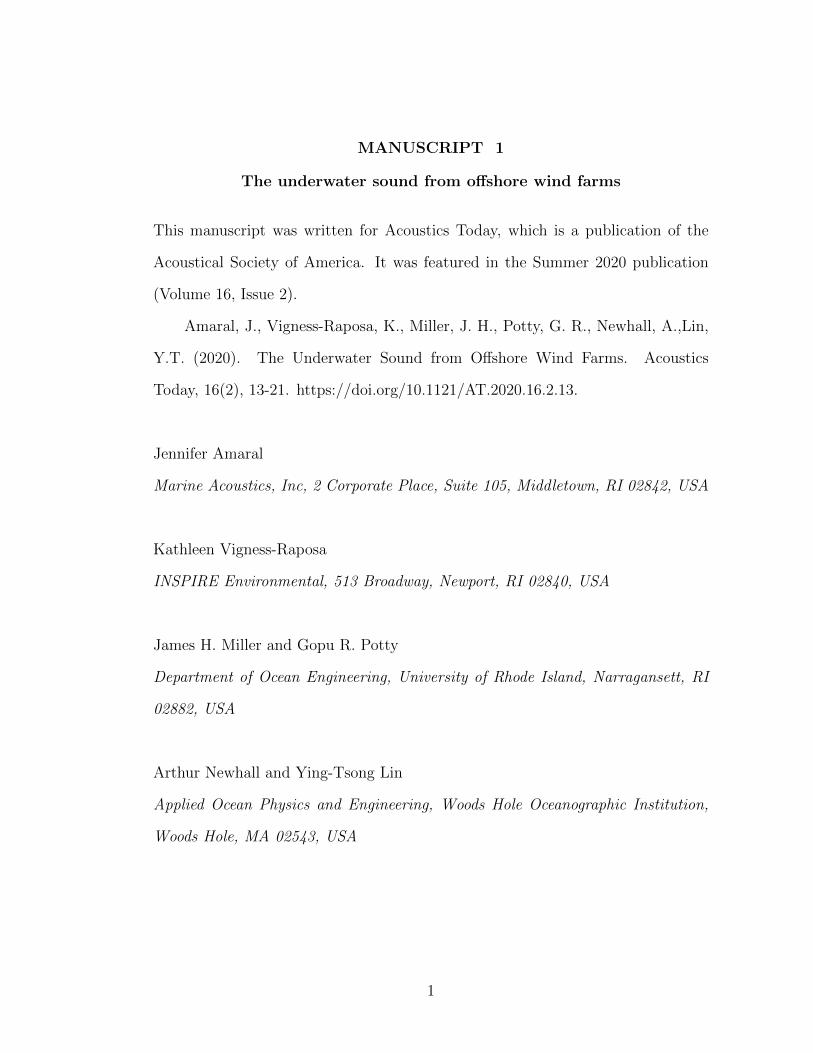
MANUSCRIPT 1
The underwater sound from offshore wind farms
This manuscript was written for Acoustics Today, which is a publication of the
Acoustical Society of America. It was featured in the Summer 2020 publication
(Volume 16, Issue 2).
Amaral, J., Vigness-Raposa, K., Miller, J. H., Potty, G. R., Newhall, A.,Lin,
Y.T. (2020). The Underwater Sound from Offshore Wind Farms. Acoustics
Today, 16(2), 13-21. https://doi.org/10.1121/AT.2020.16.2.13.
Jennifer Amaral
Marine Acoustics, Inc, 2 Corporate Place, Suite 105, Middletown, RI 02842, USA
Kathleen Vigness-Raposa
INSPIRE Environmental, 513 Broadway, Newport, RI 02840, USA
James H. Miller and Gopu R. Potty
Department of Ocean Engineering, University of Rhode Island, Narragansett, RI
02882, USA
Arthur Newhall and Ying-Tsong Lin
Applied Ocean Physics and Engineering, Woods Hole Oceanographic Institution,
Woods Hole, MA 02543, USA
1

1.1 Introduction
Efforts to reduce carbon emissions from the burning of fossil fuels have led to
an increased interest in renewable energy sources from around the globe. Offshore
wind is a viable option to provide energy to coastal communities and has many ad-
vantages over onshore wind energy production due to the limited space constraints
and greater resource potential found offshore. The first offshore wind farm was
installed off the coast of Denmark in 1991, and since then numerous others have
been installed worldwide. At the end of 2017, there were 18,814 megawatts (MW)
of installed offshore wind capacity worldwide, with nearly 84% of all installations
located in European waters and the remaining 16% located offshore of China, fol-
lowed by Vietnam, Japan, South Korea, the United States, and Taiwan. This
equated to 4,149 grid-connected offshore wind turbines in Europe alone, with the
number increasing annually since then (Global Wind Energy Council, 2017). In
the last 10 years, the average size of European offshore wind farms has increased
from 79.6 MW in 2007 to 561 MW in 2018 (Wind Europe, 2018).
On land, China leads the onshore wind energy market with 206 gigawatts
(GW) of installed capacity, followed by the United States with 96 GW in 2018
(Global Wind Energy Council, 2019). Over 80% of the US electricity demand
is from coastal states, but onshore wind energy generation is usually located far
from these coastal areas, which results in long-distance energy transmission. With
over 2,000 GW of offshore wind energy potential in US waters, which equals nearly
double the electricity demand of the nation, offshore development could provide an
alternative to long-distance transmission or development of onshore installations
in land-constrained coastal regions (US Department of Energy, 2016). With the
potential for offshore wind to be a clean and affordable renewable energy source, US
federal and state government interest in development is continuing to grow. The
2
US Bureau of Ocean Energy Management (BOEM) is responsible for overseeing
all the offshore renewable energy development on the outer continental shelf of the
United States, which includes issuing leases and providing approval for all potential
wind energy projects.
The Block Island Wind Farm (BIWF) was completed in 2016 off the East
Coast of the United States in Rhode Island and is the first and only operational
wind farm in US waters to date. It produces 30 MW from five 6-MW turbines
and is capable of powering about 17,000 homes. As of August 2019, there were
15 additional active offshore wind leases that account for over 21 GW of potential
capacity off the East Coast of the United States.
Offshore wind farms are generally constructed in shallow coastal waters, which
often have a high biological productivity that attracts diverse marine life. The av-
erage water depth of wind farms under construction in 2018 in European waters
was 27.1 meters and the average distance to shore was 33 kilometers (Wind Europe,
2018). As a by-product of the construction, operation, and eventual decommis-
sioning of offshore wind farms, sound is generated both in air and underwater
through various activities and mechanisms. With the rate of wind farm develop-
ment continuing to increase worldwide, regulatory agencies, industry, and scien-
tists are attentive to the potential physiological and behavioral effects these sounds
might have on marine life living in the surrounding environment. The contribution
of sound produced during any anthropogenic activity can change the underwater
soundscape and alter the habitats of marine mammals, fishes, and invertebrates
by potentially masking communications for species that rely on sound for mating,
navigating, and foraging. This article discusses the typical sounds produced during
the life of a wind farm, efforts that can be taken to reduce sound levels, and how
these sounds might be assessed for their potential environmental impact.
3

1.2 Construction of Offshore Wind Turbines
Once the development of a wind farm has been approved, the installation of
the wind turbine foundations can begin. The type of foundation used will depend
on parameters such as the water depth, seabed properties at the site, and turbine
size. In water depths less than 50 meters, fixed foundations such as monopiles,
gravity base, and jacket foundations are used to secure the wind turbines to the
seabed (Figure 1.1). A gravity base foundation is a type of reinforced concrete
structure used in water depths less than 10 meters that sits on the seabed and is
heavy enough to keep the wind turbine upright. A monopile foundation is a single
steel tube with a typical diameter of 3-8 meters that is driven into the seafloor,
whereas a jacket foundation is a steel structure composed of many smaller tubular
members welded together that sits on top of the seafloor and is secured by multiple
steel piles driven into the sediment (Wu et al., 2019). Monopiles can be driven to a
depth of 20-45 meters below the seafloor and the piles to secure jacket foundations
that can be driven to a depth of between 30 and 75 meters (JASCO and LGL,
2019).
4

Figure 1.1. Schematic showing some types of offshore wind turbine foundationstructures, with the wind turbine components labeled. Image courtesy of theBureau of Safety and Environmental Enforcement (BSEE), Department of theInterior (see https://tinyurl.com/wawb979).
Most installed wind turbines utilize bottom-fixed foundations, but these foun-
dations become less feasible in water depths greater than 50 meters. In the United
States, roughly 58% of the offshore wind potential is in water depths deeper than
60 meters (US Department of Energy, 2016). In these greater water depths, float-
ing foundations that are tethered to the seabed using anchors are a more viable
option.
1.3 Impact Pile Driving
Impact pile driving, where the top of the pile is pounded repeatedly by a heavy
hammer, is a method used to install monopile and jacket foundations and generates
sound in the air, water, and sediment. The installation of a jacket foundation
requires multiple piles be driven into the seabed to secure the corners of the steel
structure, whereas installation of the monopile design requires one larger pile be
driven (Norro et al., 2013). Pile driving is not used for the installation of floating
or gravity-based foundations and therefore is not an inherent part of wind farm
construction if the water depths and sediment characteristics at the installation
5
site are suitable for these alternate foundations.
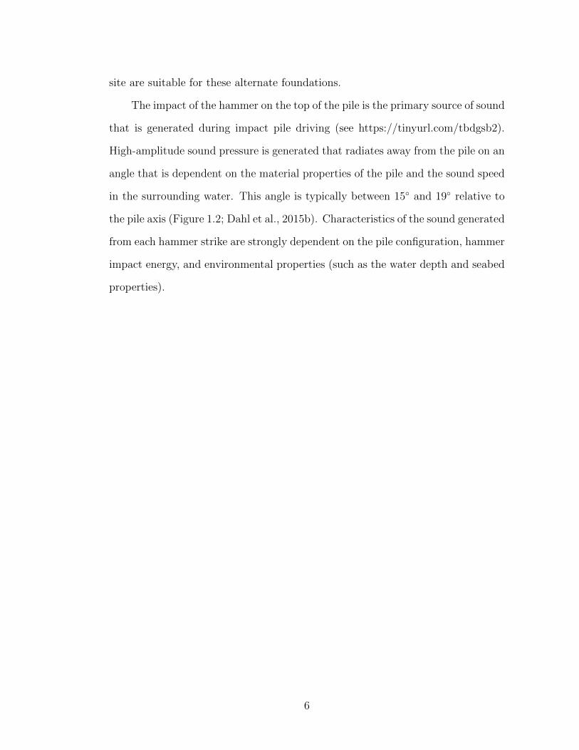
The impact of the hammer on the top of the pile is the primary source of sound
that is generated during impact pile driving (see https://tinyurl.com/tbdgsb2).
High-amplitude sound pressure is generated that radiates away from the pile on an
angle that is dependent on the material properties of the pile and the sound speed
in the surrounding water. This angle is typically between 15◦ and 19◦ relative to
the pile axis (Figure 1.2; Dahl et al., 2015b). Characteristics of the sound generated
from each hammer strike are strongly dependent on the pile configuration, hammer
impact energy, and environmental properties (such as the water depth and seabed
properties).
6
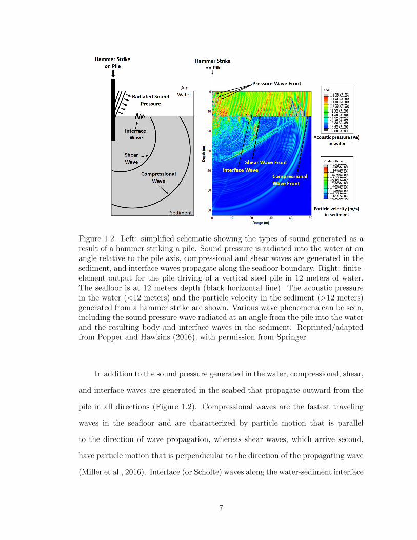
Figure 1.2. Left: simplified schematic showing the types of sound generated as aresult of a hammer striking a pile. Sound pressure is radiated into the water at anangle relative to the pile axis, compressional and shear waves are generated in thesediment, and interface waves propagate along the seafloor boundary. Right: finite-element output for the pile driving of a vertical steel pile in 12 meters of water.The seafloor is at 12 meters depth (black horizontal line). The acoustic pressurein the water (<12 meters) and the particle velocity in the sediment (>12 meters)generated from a hammer strike are shown. Various wave phenomena can be seen,including the sound pressure wave radiated at an angle from the pile into the waterand the resulting body and interface waves in the sediment. Reprinted/adaptedfrom Popper and Hawkins (2016), with permission from Springer.
In addition to the sound pressure generated in the water, compressional, shear,
and interface waves are generated in the seabed that propagate outward from the
pile in all directions (Figure 1.2). Compressional waves are the fastest traveling
waves in the seafloor and are characterized by particle motion that is parallel
to the direction of wave propagation, whereas shear waves, which arrive second,
have particle motion that is perpendicular to the direction of the propagating wave
(Miller et al., 2016). Interface (or Scholte) waves along the water-sediment interface
7

occur as a result of interfering compressional and shear waves. The low-frequency
and slow-moving interface waves propagate over long distances and generate large-
amplitude oscillations along the water-sediment boundary that have the potential
to affect marine life living close to or within the seafloor sediment that is sensitive
to this type of disturbance (Popper and Hawkins, 2018). The amplitude of the
interface wave decays exponentially away from the interface, and, therefore, any
disturbance will be noticeable only within a distance of a few wavelengths from
the seafloor (Tsouvalas and Metrikine, 2016).
1.3.1 Measuring the Radiated Sound
The total number of hammer strikes required to drive a pile to its final penetra-
tion depth could range between 500 to more than 5,000, with the hammer striking
the pile between 15 and 60 times per minute (Matuschek and Betke, 2009). On
average, a jacket foundation requires three times more hammer strikes to install
than a monopile and will result in a longer total piling time because the jacket
design requires multiple piles to secure the structure to the seabed as opposed
to a single pile for the monopile design (Norro et al., 2013). To characterize the
impulsive sound generated during each hammer strike as part of impact pile driv-
ing, the sound exposure level (SEL) and peak sound pressure level metrics can
be used. The SEL is a measure of the energy within a signal and allows for the
total energy of sounds with different durations to be compared. It is defined as the
time integral of the squared sound pressure reported in units of decibels re 1µPa2s.
This metric can be used to describe the sound levels from a single strike (SELss)
and cumulated across multiple hammer strikes or over the duration of the piling
activity (SELcum). When assessing the potential effect of impulsive sounds on the
physiology of marine mammals and fishes, the peak sound pressure level and SEL
are used (Popper et al., 2014; Southall et al., 2019).
8
A standard measurement method is important to ensure that independent
measurements made at different wind farms can be compared. An approach for
measuring and characterizing the underwater sound generated during impact pile
driving is defined through the International Organization of Standardization (ISO)
18406 document (2017), which is the standard for measurements of radiated un-
derwater sound from impact pile driving. In this standard, a combination of range-
varying hydrophone deployments and fixed-range measurements are recommended
to capture variation in the resulting sound field with both distance and changing
source characteristics. The source characteristics and resulting sound level radi-
ated into the environment will vary during a piling sequence due to changes in the
hammer strike energy, penetration depth of the pile, and depth-dependent seabed
properties. Usually, the piling event will begin with hammer strikes at a lower
energy before increasing to a higher strike energy to drive the pile deeper into the
seafloor. As the length of the pile driven into the seafloor increases, it has the po-
tential to encounter sediment layers with different properties that would influence
the resulting radiated sound levels. This variation could be adequately captured
on stationary measurement systems, ideally deployed at multiple ranges but with
at least one deployed at a range of 750 meters to facilitate comparison with the
large number of existing measurements at this range from other wind farm sites
(Robinson and Theobald, 2017).
1.3.2 Frequency Content of Hammer Strikes
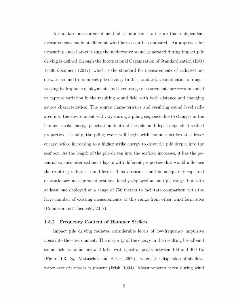
Impact pile driving radiates considerable levels of low-frequency impulsive
noise into the environment. The majority of the energy in the resulting broadband
sound field is found below 2 kHz, with spectral peaks between 100 and 400 Hz
(Figure 1.3, top; Matuschek and Betke, 2009) , where the dispersion of shallow-
water acoustic modes is present (Frisk, 1994). Measurements taken during wind
9
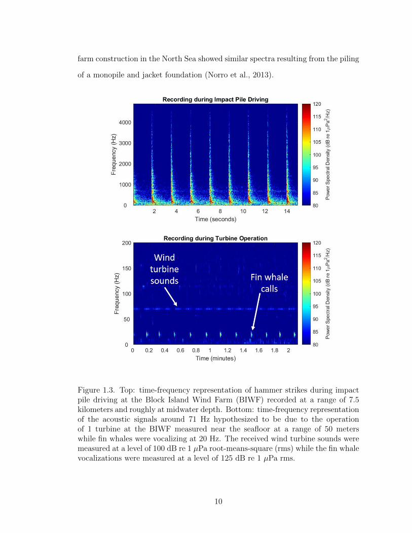
farm construction in the North Sea showed similar spectra resulting from the piling
of a monopile and jacket foundation (Norro et al., 2013).
Figure 1.3. Top: time-frequency representation of hammer strikes during impactpile driving at the Block Island Wind Farm (BIWF) recorded at a range of 7.5kilometers and roughly at midwater depth. Bottom: time-frequency representationof the acoustic signals around 71 Hz hypothesized to be due to the operationof 1 turbine at the BIWF measured near the seafloor at a range of 50 meterswhile fin whales were vocalizing at 20 Hz. The received wind turbine sounds weremeasured at a level of 100 dB re 1 µPa root-means-square (rms) while the fin whalevocalizations were measured at a level of 125 dB re 1 µPa rms.
10

1.3.3 Azimuthal Dependence of Radiated Sound Fields
The installation of jacket foundations sometimes requires piles to be driven
on an angle inside the legs of the foundation. For example, the legs of the jacket
foundations at the BIWF were hollow, steel members that were inclined inward at
an angle of roughly 13◦ and piles were impact driven into the legs to secure the
foundation to the seabed (Figure 4). The nonaxisymmetric orientation of the pile
relative to the seabed causes an azimuthal dependence to the radiated sound field,
which can result in a significant variation in the received sound levels measured
along different radials (Wilkes and Gavrilov, 2017). Received levels recorded on
fixed-range and towed measurement systems were substantially different (≈10 dB)
between piles inclined in opposite directions (Vigness-Raposa et al., 2017; Mar-
tin and Barclay, 2019). These differences were observed independent of the strike
energy used for individual hammer strikes (Amaral et al., 2020). The pile orienta-
tion affected the incident angle of the radiated pressure wave front on the seabed,
which resulted in the directivity of the radiated sound varying based on the az-
imuth. The steeper the incident angle of the radiated wave front on the seafloor,
the more energy was absorbed in the sediment. The azimuthal dependence to the
radiated sound field and resulting sound levels are important factors to consider
when determining the potential marine mammal and fish impact zones around
pile-driving activities for inclined piles.
1.4 Vibratory Pile Driving
Vibratory pile driving is another method used to drive piles into the seafloor
and could be used prior to impact pile driving to ensure that the pile is sta-
ble in the seabed (JASCO and LGL, 2019) or for the installation of sheet piles
to construct temporary cofferdams (Tetra Tech, 2012). In this process, the pile
is vibrated at a certain frequency, typically between 20 and 40 Hz, to drive it
11
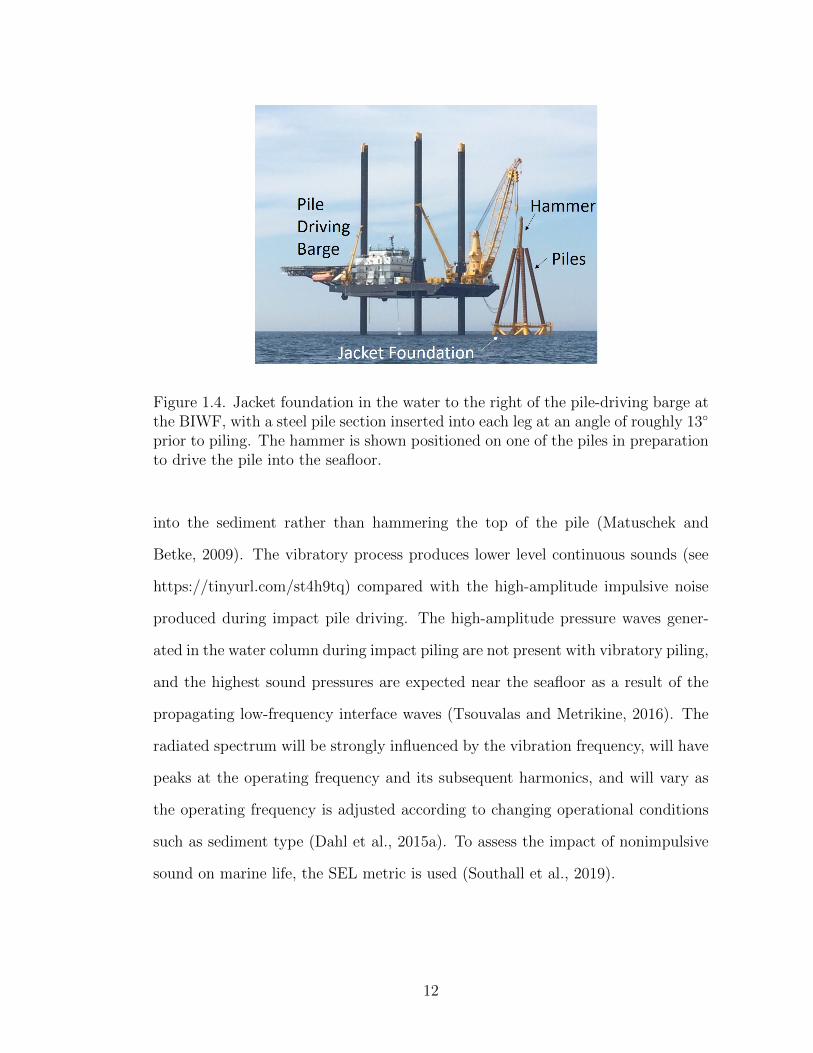
Figure 1.4. Jacket foundation in the water to the right of the pile-driving barge atthe BIWF, with a steel pile section inserted into each leg at an angle of roughly 13◦
prior to piling. The hammer is shown positioned on one of the piles in preparationto drive the pile into the seafloor.
into the sediment rather than hammering the top of the pile (Matuschek and
Betke, 2009). The vibratory process produces lower level continuous sounds (see
https://tinyurl.com/st4h9tq) compared with the high-amplitude impulsive noise
produced during impact pile driving. The high-amplitude pressure waves gener-
ated in the water column during impact piling are not present with vibratory piling,
and the highest sound pressures are expected near the seafloor as a result of the
propagating low-frequency interface waves (Tsouvalas and Metrikine, 2016). The
radiated spectrum will be strongly influenced by the vibration frequency, will have
peaks at the operating frequency and its subsequent harmonics, and will vary as
the operating frequency is adjusted according to changing operational conditions
such as sediment type (Dahl et al., 2015a). To assess the impact of nonimpulsive
sound on marine life, the SEL metric is used (Southall et al., 2019).
12
1.5 Additional Construction-Related Sounds
The construction of an offshore wind project generates sound during other
activities apart from pile driving, including during the laying of electric cables on
the seabed and from the operation of the vessels used during construction. The
primary source of noise during the cable laying process is from vessel operations
and the potential use of dynamic positioning thrusters to hold vessels in position.
An environmental assessment performed for the Vineyard Wind project off the
coast of Massachusetts concluded that the sounds generated from these activities
were generally consistent with those from routine vessel traffic expected in the
area, and, therefore, they were not anticipated to be a significant contributor to
the overall acoustic footprint of the project (JASCO and LGL, 2019).
1.6 Operational Sounds of Wind Turbines
The construction of a wind farm takes place over a period of months, whereas
the typical wind farm life span is between 20 and 25 years. Once completed,
the turbines will operate nearly continuously, except for occasional shutdowns for
maintenance or severe weather. Therefore, the contribution of sound to the marine
environment will be more consistent and of longer duration during the operational
phase than during any other phase of the life of the wind farm (Nedwell and Howell,
2004). The underwater noise levels emitted during the operation of the turbines
are low and not expected to cause physiological injury to marine life but could
cause behavioral reactions if the animals are in the immediate vicinity of the wind
turbine (Tougaard et al., 2009; Sigray and Andersson, 2011).
In some shallow-water environments, sound due to shipping traffic or storms
could dominate the low-frequency ambient-sound field over the sound emitted from
the wind turbines. Therefore, evaluating the relative sound levels from the wind
turbine compared with those from other sources is important when considering
13
the potential impacts to marine life. Measurements made at three different wind
turbines in Denmark and Sweden at ranges between 14 and 40 meters from the tur-
bine foundations found that the sound generated due to turbine operation was only
detectable over underwater ambient noise at frequencies below 500 Hz (Tougaard
et al., 2009).
The main sources of sound generated during the operation of wind turbines
are aerodynamic and mechanical. The mechanical noise is from the nacelle, which
is situated at the top of the wind turbine tower and houses the gear box and
generator (Figure 1.1). As the wind turbine blades rotate, vibrations are gen-
erated that travel down the turbine tower into the foundation and radiate into
the surrounding water column and seabed (Tougaard et al., 2009). The result-
ing sound is described as continuous and nonimpulsive and is characterized by
one or more tonal components that are typically at frequencies below 1 kHz (see
https://tinyurl.com/wke3lso). The frequency content of the tonal signals is deter-
mined by the mechanical properties of the wind turbine and does not change with
wind speed (Madsen et al., 2006).
Underwater measurements taken during the operation of one of the turbines at
the BIWF contained sound that is hypothesized to be caused by aerodynamic noise
from the turbine blade tips that was propagated through the air, into the water,
and received on a hydrophone on the seabed at a range of 50 meters (Figure 1.3,
bottom; J. Miller, Personal observation). This sound was measured to be around
71 Hz and was lower in level than fin whale vocalizations recorded at the same
time. This sound was only detectable during times when the weather was calm
and there were no ships traveling in the area.
14
1.7 Sounds from Decommissioning
Since the first offshore wind farm decommissioning in 2015, a small number
of offshore farms have been decommissioned, but the decommissioning process is
generally unexplored. As more wind farms reach the end of their design life, the
decision will have to be made relating to extending operations, repowering, or de-
commissioning. Decommissioning is typically thought of as a complete removal
of all components above and below the water surface, but there is research sup-
porting a partial removal where some of the substructure would remain in place
as an artificial reef for marine life (Topham et al., 2019). In general, sound would
be generated as a by-product of the process used to remove the substructures,
which could include cutting the foundation piles via explosives or water jet cutting
(Nedwell and Howell, 2004).
1.8 Assessing Impact to Marine Life
Impulsive sounds, like those generated during impact pile driving, exhibit
physical characteristics at the source that make them potentially more injurious to
marine life compared with nonimpulsive sounds, like those generated during vibra-
tory pile driving and wind turbine operation (Popper et al., 2014; Southall et al.,
2019). Sound exposure is currently assessed based on the sound pressure received
in the water column, but the resulting particle motion in the water and sediment
is also important when considering the potential impact to marine life sensitive
to this stimulus. Additionally, the context under which an animal is exposed to
a sound, in addition to the received sound level, will affect the probability of a
behavioral response (Ellison et al., 2012).
15
1.9 Protective Measures to Mitigate Sound Levels
Various mitigation methods can be employed during each phase of wind farm
development to reduce the overall propagated sound levels and potential effect on
marine life. Time-of-year limitations on construction are implemented to provide
safeguards for specific protected or susceptible species. Anti-noise legislation in the
Netherlands prohibits pile driving from July 1 through December 31 to avoid dis-
turbance of the breeding season of the harbor porpoise (Tsouvalas and Metrikine,
2016). Off the US East Coast, an agreement was made between environmental
groups and a wind farm developer to provide protections for the North Atlantic
right whale by not allowing pile driving between January 1 and April 30 when
right whales are most likely to be present in the project area (Conservation Law
Foundation, 2019).
The use of noise mitigation systems such as bubble curtains (see
https://tinyurl.com/v6m6ops) or physical barriers around the pile are commonly
used to reduce the levels of sound generated during impact pile driving (Bellmann
et al., 2017). These methods are a type of barrier system that work to attenu-
ate the radiated sound levels by exploiting an impedance mismatch between the
generated sound wave and a gas-filled barrier. Factors such as the water depth,
current, and foundation type will influence the effectiveness of each system.
Ramp-up operational mitigation measures, in which the hammer intensity
is gradually increased to full power, are also employed. This method aims to
allow time for animals to leave the immediate area and avoid exposure to harmful
sound levels, although there are no data to support the contention that this works
for fishes, invertebrates, or turtles. Another mitigation method involves visually
monitoring an exclusion zone around the piling activity for the presence of marine
mammals. This zone is predefined based on the expected sound levels in the area
16

and requires pausing piling activities if an animal is observed to reduce near-field
noise exposure (Bailey et al., 2014).
Exploiting seasonal differences in the water temperature and salinity and its
effect on underwater sound propagation could also be used to mitigate the impact
of pile-driving noise by scheduling wind farm construction during seasons of high
expected acoustic transmission loss. For example, the pile driving for the BIWF
occurred during the summer season but had the construction occurred during the
winter season, the received SELs at ranges greater than 6 kilometers could have
been up to 8 dB higher (Figure 1.5) due to lower water temperatures causing
larger acoustic impedance contrast at the seafloor (water-bottom interface) and a
more isovelocity, or constant, sound speed profile (Lin et al., 2019). This difference
in received sound levels is significant and highlights the effect the environmental
conditions have on the overall sound propagation.
17

Figure 1.5. Seasonal variability of underwater sound propagation in the BIWF areashowing transmission loss (TL) predictions in decibels for a 200 Hz sound sourcein September 2015 (summer; a) and December 2015 (winter; b). The source depth(Zs) in the model was 15 meters and the receiver depth (Zr) was 20 meters. Thecorresponding sound speed profiles (SSP) are shown. The TL was higher in thesummer compared with the winter conditions. Reproduced from Lin et al. (2019),with permission.
1.10 Conclusion
Ancillary sounds of varying levels and characteristics are generated during
each phase in the development of an offshore wind farm. The highest amplitude
sound is expected during the impact pile-driving part of the construction phase
and potentially during the decommissioning phase depending on the methods em-
ployed to remove the wind turbine foundations. The installation methods used
18

for each turbine foundation type will result in different levels and types of sounds
radiated into the marine environment. The sound levels can be reduced using
physical barriers, and the sound exposure of marine life can be mitigated through
monitoring methods and time-of-year restrictions on sound-generating activities.
The potential for acute sound exposure of marine mammals and fishes is currently
assessed based on the generated sound pressure levels in the water column, but
other factors such as the particle motion in the water and sediment and the be-
havioral response of marine life are important factors to evaluate. Although the
construction and decommissioning phases take on the order of months to complete,
offshore wind farms are designed to operate for minimum of 20-25 years. With the
continued development of offshore wind farms worldwide there will be additional
opportunities to measure the underwater sound generated during all phases and
assess any potential long-term effect of this sound on the marine environment.
19

Bibliography
Amaral, J. L., Miller, J. H., Potty, G. R., Vigness-Raposa, K. J., Frankel, A. S.,
Lin, Y.-T., Newhall, A. E., Wilkes, D. R., and Gavrilov, A. N. (2020). Character-
ization of impact pile driving signals during installation of offshore wind turbine
foundations. The Journal of the Acoustical Society of America, 147(4):2323–
2333.
Bailey, H., Brookes, K. L., and Thompson, P. M. (2014). Assessing environmental
impacts of offshore wind farms: Lessons learned and recommendations for the
future. Aquatic Biosystems, 10(1):1–13.
Bellmann, M. A., Schuckenbrock, J., Gundert, S., Michael, M., Holst, H., and
Remmers, P. (2017). Is There a State-of-the-Art to Reduce Pile-Driving Noise?
Wind Energy and Wildlife Interactions.
Conservation Law Foundation (2019). Protective Measures for North Atlantic
Right Whales.
Dahl, P. H., Dall’Osto, D. R., and Farrell, D. M. (2015a). The underwater sound
field from vibratory pile driving. The Journal of the Acoustical Society of Amer-
ica, 137(6):3544–3554.
Dahl, P. H., de Jong, C. A., and Popper, A. N. (2015b). The Underwater Sound
Field from Impact Pile Driving and Its Potential Effects on Marine Life. Acous-
tics Today, 11(2):18–25.
Ellison, W. T., Southall, B. L., Clark, C. W., and Frankel, A. S. (2012). A New
Context-Based Approach to Assess Marine Mammal Behavioral Responses to
Anthropogenic Sounds. Conservation Biology, 26(1):21–28.
20

Frisk, G. V. (1994). Ocean and Seabed Acoustics. Prentice-Hall, Inc, Englewood
Cliffs, New Jersey.
Global Wind Energy Council (2017). GWEC Global Wind 2017 Report - A snap-
shot of top wind markets in 2017: Offshore wind. Technical report, Global Wind
Energy Council.
Global Wind Energy Council (2019). Global Wind Report 2018. Technical Report
April, Global Wind Energy Council, Brussels, Belgium.
ISO (2017). ISO 18406 Underwater acoustics - Measurement of radiated underwa-
ter sound from percussive pile driving. International Organization for Standard-
ization, Geneva, Switzerland.
JASCO and LGL (2019). Request for an Incidental Harassment Authorization
to Allow the Nonlethal Take of Marine Mammals Incidental to Construction
Activities in the Vineyard Wind BOEM Lease Area OCS. Technical report,
Prepared by JASCO Applied Sciences (USA) Ltd. and LGL Ecological Research
Associates, for Vineyard Wind, LLC, Version 4.1, Document No. 01648.
Lin, Y.-T., Newhall, A. E., Miller, J. H., Potty, G. R., and Vigness-Raposa, K. J.
(2019). A three-dimensional underwater sound propagation model for offshore
wind farm noise prediction. The Journal of the Acoustical Society of America,
145(5):EL335–EL340.
Madsen, P. T., Wahlberg, M., Tougaard, J., Lucke, K., and Tyack, P. (2006). Wind
turbine underwater noise and marine mammals: Implications of current knowl-
edge and data needs. Marine Ecology Progress Series, 309(Tyack 1998):279–295.
Martin, S. B. and Barclay, D. R. (2019). Determining the dependence of marine
pile driving sound levels on strike energy , pile penetration , and propagation
21

effects using a linear mixed model based on damped cylindrical spreading. The
Journal of the Acoustical Society of America, 146(1):109–121.
Matuschek, R. and Betke, K. (2009). Measurements of Construction Noise During
Pile Driving of Offshore Research Platforms and Wind Farms. NAG/DAGA
International Conference on Acoustics, pages 262–265.
Miller, J. H., Potty, G. R., and Kim, H.-K. (2016). Pile-Driving Pressure and Parti-
cle Velocity at the Seabed: Quantifying Effects on Crustaceans and Groundfish.
In Popper, A. N. and Hawkins, A. D., editors, The Effects of Noise on Aquatic
Life II, New York, NY. Springer.
Nedwell, J. and Howell, D. (2004). A review of offshore windfarm related under-
water noise sources.
Norro, A. M. J., Rumes, B., and Degraer, S. J. (2013). Differentiating between
Underwater Construction Noise of Monopile and Jacket Foundations for Offshore
Windmills: A Case Study from the Belgian Part of the North Sea. The Scientific
World Journal, pages 1–7.
Popper, A. N. and Hawkins, A. D., editors (2016). The Effects of Noise on Aquatic
Life II. Springer, New York, NY.
Popper, A. N. and Hawkins, A. D. (2018). The importance of particle motion
to fishes and invertebrates. The Journal of the Acoustical Society of America,
143(1):470–488.
Popper, A. N., Hawkins, A. D., Fay, R. R., Mann, D. A., Bartol, S., Carlson,
T. J., Coombs, S., Ellison, W. T., Gentry, R. L., Halvorsen, M. B., Løkkeborg, S.,
Rogers, P. H., Southall, B. L., Zeddies, D. G., and Tavolga, W. N. (2014). Sound
Exposure Guidelines for Fishes and Sea Turtles: A Technical Report prepared by
22

ANSI-Accredited Standards Committee S3/SC1 and registered with ANSI. ASA
S3/SC1.4 TR-2014. Springer International Publishing, Cham, Switzerland.
Robinson, S. P. and Theobald, P. (2017). A Standard for the Measurement of Un-
derwater Sound Radiated from Marine Pile Driving. 24th International Congress
on Sound and Vibration.
Sigray, P. and Andersson, M. H. (2011). Particle motion measured at an opera-
tional wind turbine in relation to hearing sensitivity in fish. The Journal of the
Acoustical Society of America, 130.
Southall, B. L., Finneran, J. J., Reichmuth, C., Nachtigall, P. E., Ketten, D. R.,
Bowles, A. E., Ellison, W. T., Nowacek, D. P., and Tyack, P. L. (2019). Ma-
rine Mammal Noise Exposure Criteria: Updated Scientific Recommendations
for Residual Hearing Effects. Aquatic Mammals, 45(2):125–232.
Tetra Tech (2012). Block Island Wind Farm and Block Island Transmission System
Environmental Report / Construction and Operations Plan. Technical report,
Submitted by Deepwater Wind, Boston, MA.
Topham, E., Gonzalez, E., McMillan, D., and Joao, E. (2019). Challenges of
decommissioning offshore wind farms: Overview of the European experience. In
Journal of Physics: Conference Series, volume 1222.
Tougaard, J., Henriksen, O. D., and Miller, L. A. (2009). Underwater noise from
three types of offshore wind turbines: Estimation of impact zones for harbor
porpoises and harbor seals. The Journal of the Acoustical Society of America,
125(6):3766–3773.
Tsouvalas, A. and Metrikine, A. V. (2016). Structure-Borne Wave Radiation by
23
Impact and Vibratory Piling in Offshore Installations : From Sound Prediction
to Auditory Damage. Journal of Marine Science and Engineering.
US Department of Energy (2016). National offshore wind strategy - facilitating
the development of the offshore wind industry in the US. Technical report, US
Department of Energy.
Vigness-Raposa, K. J., Giard, J. L., Frankel, A. S., Miller, J. H., Potty, G. R., Lin,
Y.-T., Newhall, A. E., and Mason, T. (2017). Variations in the acoustic field
recorded during pile-driving construction of the Block Island Wind Farm. The
Journal of the Acoustical Society of America, 141.
Wilkes, D. R. and Gavrilov, A. N. (2017). Sound radiation from impact-driven
raked piles. Journal of the Acoustical Society of America, 142(1):1–11.
Wind Europe (2018). Offshore wind in Europe. Technical report, Wind Europe.
Wu, X., Hu, Y., Li, Y., Yang, J., Duan, L., Wang, T., Adcock, T., Jiang, Z., Gao,
Z., Lin, Z., Borthwick, A., and Liao, S. (2019). Foundations of offshore wind
turbines: A review. Renewable and Sustainable Energy Reviews, 104:379–393.
24

MANUSCRIPT 2
Characterization of impact pile driving signals during installation ofoffshore wind turbine foundations
This manuscript was written for publication in the Journal of the Acoustical Soci-
ety of America as part of a special issue on The Effects of Noise on Aquatic Life.
It was accepted for publication on March 19, 2020 and published online on April
17, 2020.
Amaral, J. L., Miller, J. H., Potty, G. R., Vigness-Raposa, K. J., Frankel, A.
S., et al. (2020). Characterization of impact pile driving signals during installation
of offshore wind turbine foundations. The Journal of the Acoustical Society of
America, 147(4), 2323-2333. https://doi.org/10.1121/10.0001035.
Jennifer L. Amaral, James H. Miller and Gopu R. Potty
Department of Ocean Engineering, University of Rhode Island, Narragansett, RI
02882, USA
Kathleen J. Vigness-Raposa and Adam S. Frankel
Marine Acoustics, Inc, 2 Corporate Place, Suite 105, Middletown, RI 02842, USA
Ying-Tsong Lin and Arthur E. Newhall
Applied Ocean Physics and Engineering, Woods Hole Oceanographic Institution,
Woods Hole, MA 02543, USA
Daniel R. Wilkes and Alexander N. Gavrilov
Centre for Marine Science and Technology, School of Earth and Planetary Sciences,
Curtin University, GPO Box U1987, Perth, Western Australia 6845, Australia
25
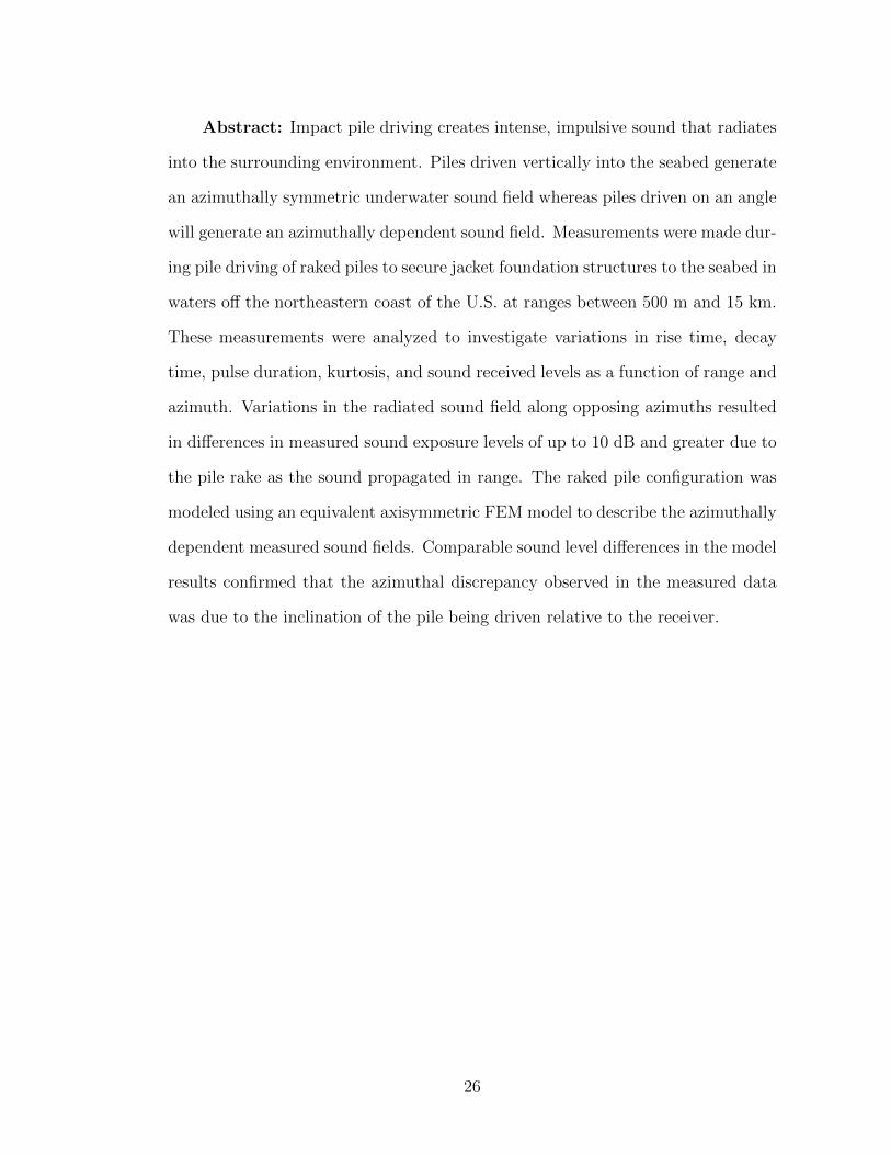
Abstract: Impact pile driving creates intense, impulsive sound that radiates
into the surrounding environment. Piles driven vertically into the seabed generate
an azimuthally symmetric underwater sound field whereas piles driven on an angle
will generate an azimuthally dependent sound field. Measurements were made dur-
ing pile driving of raked piles to secure jacket foundation structures to the seabed in
waters off the northeastern coast of the U.S. at ranges between 500 m and 15 km.
These measurements were analyzed to investigate variations in rise time, decay
time, pulse duration, kurtosis, and sound received levels as a function of range and
azimuth. Variations in the radiated sound field along opposing azimuths resulted
in differences in measured sound exposure levels of up to 10 dB and greater due to
the pile rake as the sound propagated in range. The raked pile configuration was
modeled using an equivalent axisymmetric FEM model to describe the azimuthally
dependent measured sound fields. Comparable sound level differences in the model
results confirmed that the azimuthal discrepancy observed in the measured data
was due to the inclination of the pile being driven relative to the receiver.
26
2.1 Introduction
Impact pile driving creates intense sound that radiates into the environment
and propagates through the air, water, and sediment. Characteristics of the re-
sulting sound radiation are strongly dependent on the pile configuration, hammer
impact energy, and environmental properties at the pile location and in the sur-
rounding area. With the development of offshore wind farms globally there have
been increased opportunities to measure the underwater sound fields generated
during pile driving activities in different environments and of varying pile diame-
ters (Gottsche et al., 2015; Robinson et al., 2012; Bailey et al., 2010; De Jong and
Ainslie, 2008; Norro et al., 2013). The majority of these measurements have been
of monopiles or other vertically driven piles, while few measurements of raked (an-
gled) piles have been described (Wilkes and Gavrilov, 2017; Martin and Barclay,
2019).
The dominant source of sound that is generated during pile driving is due to
the hammer impact. For a hollow steel pile, the resulting sound field is comprised
of a series of Mach waves (Reinhall and Dahl, 2011; Dahl and Dall’Osto, 2017;
Dahl and Reinhall, 2013; Zampolli et al., 2013). The hammer strike and resulting
compression wave cause the pile to bulge outwards and deform, due to the Poisson
effect. This physical deformation propagates down the pile and acts as a moving
sound source. The resulting acoustic field consists of a series of downward- and
upward-propagating axisymmetric Mach wave cones (Kim et al., 2013; Reinhall
and Dahl, 2011).
Reinhall and Dahl (2011) and Kim et al. (2013) described the propagation
of these Mach wave cones from vertically driven piles, and Wilkes and Gavrilov
(2017) modeled the Mach cone radiating from an angled pile. The angle of the
initial Mach cone relative to the pile axis is dependent on the ratio of the sound
27
speed in water (cw) to the propagation speed of the radial deformation down the
pile (cp), which is close to the compressional wave speed in steel (Equation 2.1;
Reinhall and Dahl, 2011).
θ = sin−1(cw/cp) (2.1)
Raked piles are common in infrastructure projects because of their increased
resistance to lateral loads. Due to the non-axisymmetric geometry of the pile
relative to the seabed, raked piles are expected to radiate underwater sound with
an azimuthal dependence. Wilkes and Gavrilov (2017) and Martin and Barclay
(2019) demonstrated that sound radiation from a raked pile is significantly different
at various azimuths from the pile. Measured sound exposure levels (SELs) radiated
by piles raked at an angle of 14◦ to the vertical and inclined towards the receiver
were 10 dB lower at distances of 1.2-1.5 km than those radiated from piles inclined
away from the receiver (Wilkes and Gavrilov, 2017).
The sounds generated from impact pile driving are described as impulsive,
which exhibit physical characteristics at the source that make them potentially
more injurious to marine mammals and fishes as compared to non-impulsive sounds
(Southall et al., 2019; Popper et al., 2014). Impulsive signals are defined as short-
duration broadband sounds that consist of a peak sound pressure amplitude with a
rapid rise time to the peak followed by a decay (National Marine Fisheries Service,
2018). An impulsive signal may undergo changes due to propagation effects that
could result in the signal being perceived by animals as non-impulsive at some
other range (Southall et al., 2007, 2019; National Marine Fisheries Service, 2018).
A range at which a signal might transition from being considered impulsive to
non-impulsive was briefly identified as 3 km in draft sound exposure guidance,
but was omitted from the final guidance as more research is needed to determine
28
this range (National Marine Fisheries Service (NMFS), 2015). The consideration
of a transition range is important when applying acoustic exposure guidance as
Southall et al. (2019) recommends that the signal characteristics expected to be
received by the animal rather than those at the source dictate the exposure guid-
ance used (impulsive or non-impulsive). Since propagation is dependent on the
local environmental conditions (sound speed, bottom sediment properties, water
depth, surface roughness, etc.), defining a definitive distance that would be valid
for all propagation environments is not straightforward. Also, what measurable
signal characteristic could be used to determine when a signal has undergone that
transition?
One such metric could be kurtosis, which is a statistical measure that rep-
resents the impulsiveness of an event (National Marine Fisheries Service, 2018).
According to Hamernik et al. (2003) and Lei et al. (1994), the kurtosis of a signal,
in addition to an energy metric, is an important variable in determining hazards
to hearing and is a good predictor of the relative magnitude of acoustic trauma
between signals that differ in impulsiveness. Impulsive signals with high kurto-
sis and high instantaneous peak sound pressure may be more injurious to certain
mammals (Southall et al., 2007). Rise time is another relevant metric to describe
the temporal structure of the signal that could be tied to the impact a sound will
have (Henderson and Hamernik, 1986; Laughlin, 2005). Studies are ongoing to
determine the most appropriate metric, but the onset of damage to hearing for
impulsive sounds may be more appropriately measured by the rise time of a signal
as opposed to the kurtosis (Popper et al., 2006). Additionally, a combination of
the rise time, ratio of peak pressure to pulse duration, pulse duration, and crest
factor could all be metrics used to evaluate a change in the impulsive nature of a
signal over range (Hastie et al., 2019).
29

This study will present measurements collected from the installation of raked
piles in coastal waters at the Block Island Wind Farm (BIWF) off the coast of Block
Island, Rhode Island, USA. Steel piles were driven into the seabed to pin the jacket-
type wind turbine foundation structures at BIWF. These types of foundations were
used due to their suitability in deeper waters relative to other foundations currently
available. Jacket foundations have been used extensively in the offshore oil and gas
industry and were a cost-effective choice for the BIWF based on the robust supply
chain in the U.S for the construction and installation of these foundations. Based
on these factors, the jacket foundation was the preferred choice for the BIWF
(Tetra Tech, 2012).
The piles driven at the BIWF were raked at an angle of 13.27◦ to the vertical.
This rake resulted in the incident angle of the radiated Mach wave on the seabed
changing based on azimuth. The Mach wave generated with each hammer strike is
radiated out from the pile at an angle typically around 18◦ depending on the exact
ratio of the speed of sound in steel and the surrounding water (MacGillivray, 2018;
Dahl and Dall’Osto, 2017). The similarities between the pile rake and Mach wave
angle resulted in the sound radiating from the pile axis in the direction of the pile
inclination to be directed more towards the seafloor as opposed to the sound in
the opposite direction which was directed near horizontal into the water column.
The steeper the incident angle of the Mach wave to the seafloor, the more energy
was absorbed by the seafloor (HDR, 2018). The effect of pile rake on the resulting
sound field was evident in the received signals. This sound radiation pattern is
demonstrated in Wilkes and Gavrilov (2017) where the pile orientation is similar
to that of the BIWF.
The objective of this study was to describe the measurements collected of
pile driving at the BIWF as a function of range, azimuth, and strike energy. The
30

variation in the rise time, decay time, pulse duration, and kurtosis of the signals
was investigated to determine if there was supporting evidence to define a range at
which the signal transitioned from impulsive to non-impulsive. Martin and Barclay
(2019) presented measurements of pile driving at BIWF from stationary systems
and analyzed the data using linear mixed models based on damped cylindrical
spreading to conclude that the variability in the received level was largely due to
the pile rake. The study described in this manuscript utilizes a finite element model
to investigate the variation observed in the data from both towed and stationary
systems to further explain the conclusion that the dominant source of the sound
level variation was the inclination of the pile relative to the receiver.
The paper is organized in the following manner. Section II describes the study
location along with the measurement equipment, details of the turbine foundations
and piling activity, and analysis methods. Section III presents the data collected
and the variations observed in the measured sound levels due to the pile rake
and range. The pulse duration and kurtosis of the pile driving signals are also
discussed. Section IV includes a discussion of the observations as compared to
modeled results. Section V presents the main conclusions of this study.
2.2 Observation Methods
The location of the following study was the Block Island Wind Farm, which
is the first offshore wind farm in U.S. waters. It is a 30-megawatt wind farm that
is comprised of five 6-MW turbines located three miles southeast of Block Island,
Rhode Island in water depths of approximately 30 meters. The U.S. Bureau of
Ocean Energy Management (BOEM) funded a project to study the development
and operation of this wind farm. The goal of the project was to collect real-time
measurements of the construction and operation activities from the first federally
permitted offshore wind farm in U.S. coastal waters to allow for more accurate
31
assessments of the environmental effects and inform development of appropriate
mitigation measures.
The University of Rhode Island (URI), Marine Acoustics, Inc. (MAI) and
Woods Hole Oceanographic Institution (WHOI) were funded under this project to
investigate the acoustic pressure and particle velocity associated with the construc-
tion and operation of the wind turbines. Various stationary and towed acoustic
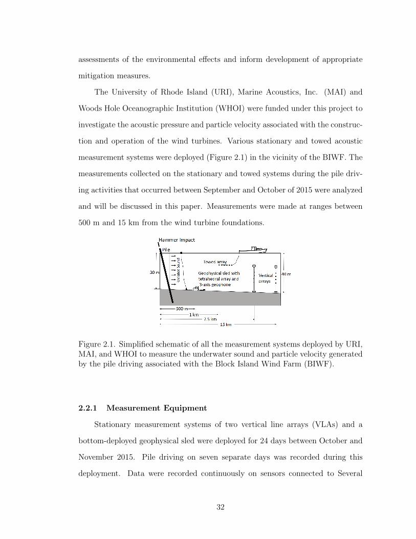
measurement systems were deployed (Figure 2.1) in the vicinity of the BIWF. The
measurements collected on the stationary and towed systems during the pile driv-
ing activities that occurred between September and October of 2015 were analyzed
and will be discussed in this paper. Measurements were made at ranges between
500 m and 15 km from the wind turbine foundations.
Figure 2.1. Simplified schematic of all the measurement systems deployed by URI,MAI, and WHOI to measure the underwater sound and particle velocity generatedby the pile driving associated with the Block Island Wind Farm (BIWF).
2.2.1 Measurement Equipment
Stationary measurement systems of two vertical line arrays (VLAs) and a
bottom-deployed geophysical sled were deployed for 24 days between October and
November 2015. Pile driving on seven separate days was recorded during this
deployment. Data were recorded continuously on sensors connected to Several
32
Hydrophone Receive Units (SHRUs) developed and maintained by WHOI. All of
the sensors were recording at a sampling rate of approximately 10 kHz for the
duration of the deployment.
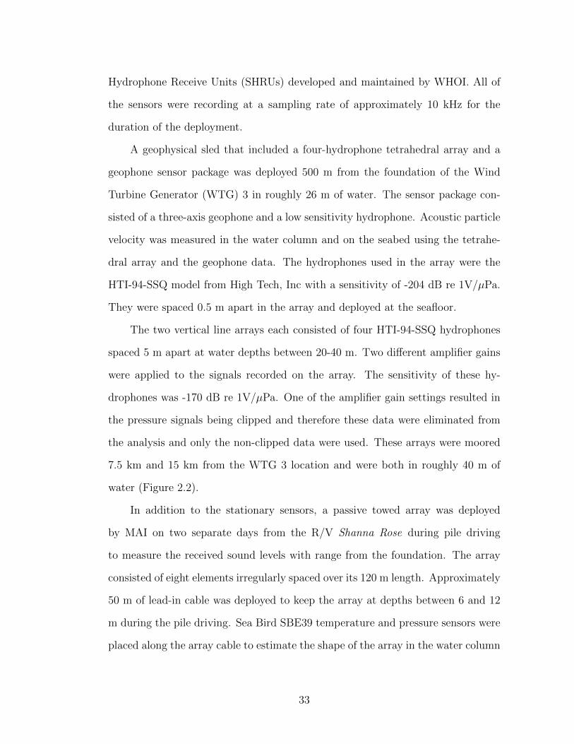
A geophysical sled that included a four-hydrophone tetrahedral array and a
geophone sensor package was deployed 500 m from the foundation of the Wind
Turbine Generator (WTG) 3 in roughly 26 m of water. The sensor package con-
sisted of a three-axis geophone and a low sensitivity hydrophone. Acoustic particle
velocity was measured in the water column and on the seabed using the tetrahe-
dral array and the geophone data. The hydrophones used in the array were the
HTI-94-SSQ model from High Tech, Inc with a sensitivity of -204 dB re 1V/µPa.
They were spaced 0.5 m apart in the array and deployed at the seafloor.
The two vertical line arrays each consisted of four HTI-94-SSQ hydrophones
spaced 5 m apart at water depths between 20-40 m. Two different amplifier gains
were applied to the signals recorded on the array. The sensitivity of these hy-
drophones was -170 dB re 1V/µPa. One of the amplifier gain settings resulted in
the pressure signals being clipped and therefore these data were eliminated from
the analysis and only the non-clipped data were used. These arrays were moored
7.5 km and 15 km from the WTG 3 location and were both in roughly 40 m of
water (Figure 2.2).
In addition to the stationary sensors, a passive towed array was deployed
by MAI on two separate days from the R/V Shanna Rose during pile driving
to measure the received sound levels with range from the foundation. The array
consisted of eight elements irregularly spaced over its 120 m length. Approximately
50 m of lead-in cable was deployed to keep the array at depths between 6 and 12
m during the pile driving. Sea Bird SBE39 temperature and pressure sensors were
placed along the array cable to estimate the shape of the array in the water column
33

Figure 2.2. Location of the vertical line arrays at 7.5 km and 15 km from the WindTurbine Generator (WTG) foundations and the geophysical sled at 500 m. Thetwo towed array transects are also shown. Bottom depth contours are indicated inmeters.
during deployment.
When towing the array, the vessel maintained a linear course away from the
foundations at a speed of approximately 1.5 m/s out to distances of 6 and 8 km
on the two days. The maximum distance was dictated by the duration of the pile
driving activity on both days. Data at ranges greater than 5 km were eliminated
from this analysis due to decreasing signal-to-noise ratio in the recorded data. The
noise was due to flow-induced turbulent pressure fluctuations on the hydrophones.
The analog output from the array was low pass filtered at 30 kHz and amplified
with an Alligator Technologies SCS-820 filter board. A National Instruments PCI-
6071E card digitized the filtered data at a sampling rate of 64 kHz. Amplifier
gains were applied during data acquisition to increase the signal amplitude as the
34
range of the array from the pile driving activity increased. Data were collected
using RAVEN Pro v 1.4 (www.birds.cornell.edu/raven) and saved in consecutive
30 second files for post-processing.
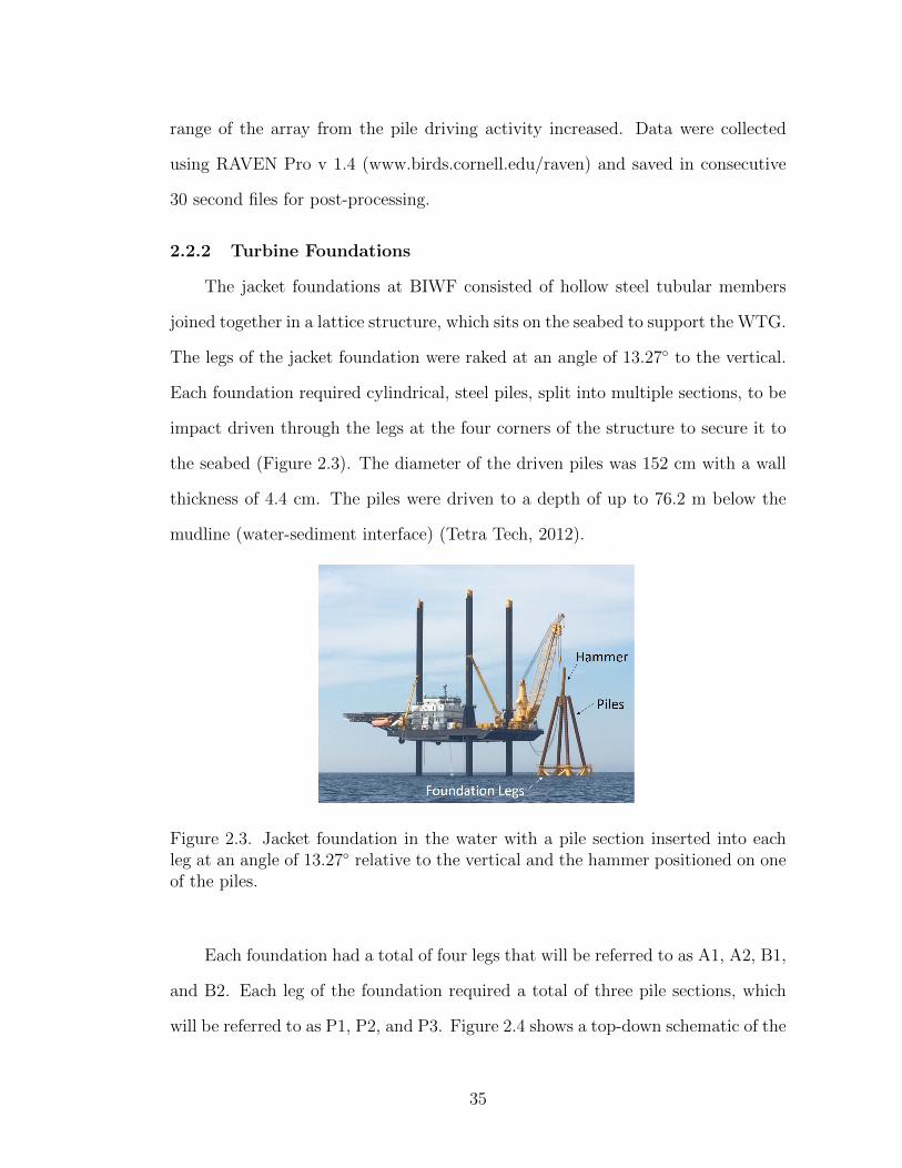
2.2.2 Turbine Foundations
The jacket foundations at BIWF consisted of hollow steel tubular members
joined together in a lattice structure, which sits on the seabed to support the WTG.
The legs of the jacket foundation were raked at an angle of 13.27◦ to the vertical.
Each foundation required cylindrical, steel piles, split into multiple sections, to be
impact driven through the legs at the four corners of the structure to secure it to
the seabed (Figure 2.3). The diameter of the driven piles was 152 cm with a wall
thickness of 4.4 cm. The piles were driven to a depth of up to 76.2 m below the
mudline (water-sediment interface) (Tetra Tech, 2012).
Figure 2.3. Jacket foundation in the water with a pile section inserted into eachleg at an angle of 13.27◦ relative to the vertical and the hammer positioned on oneof the piles.
Each foundation had a total of four legs that will be referred to as A1, A2, B1,
and B2. Each leg of the foundation required a total of three pile sections, which
will be referred to as P1, P2, and P3. Figure 2.4 shows a top-down schematic of the
35
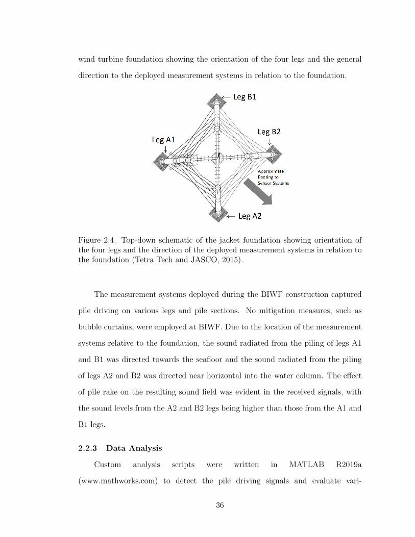
wind turbine foundation showing the orientation of the four legs and the general
direction to the deployed measurement systems in relation to the foundation.
Figure 2.4. Top-down schematic of the jacket foundation showing orientation ofthe four legs and the direction of the deployed measurement systems in relation tothe foundation (Tetra Tech and JASCO, 2015).
The measurement systems deployed during the BIWF construction captured
pile driving on various legs and pile sections. No mitigation measures, such as
bubble curtains, were employed at BIWF. Due to the location of the measurement
systems relative to the foundation, the sound radiated from the piling of legs A1
and B1 was directed towards the seafloor and the sound radiated from the piling
of legs A2 and B2 was directed near horizontal into the water column. The effect
of pile rake on the resulting sound field was evident in the received signals, with
the sound levels from the A2 and B2 legs being higher than those from the A1 and
B1 legs.
2.2.3 Data Analysis
Custom analysis scripts were written in MATLAB R2019a
(www.mathworks.com) to detect the pile driving signals and evaluate vari-
36

ous metrics of each recorded hammer strike encompassing the entire recorded
frequency range of the signals. The upper limit of the frequency content in the
signals recorded on the stationary systems was just under 5 kHz as compared to
an upper limit of 30 kHz for the towed array measurements. The peak sound
pressure level (SPLpk), sound exposure level (SEL), pulse duration, rise time,
decay time, and kurtosis of each individual hammer strike signal were calculated.
These measurements were correlated with the strike energy of the hammer to
investigate dependence on the initial strike energy and pile orientation. The
towed array data were also correlated with distance to investigate the range
dependencies of these metrics.
The sound metrics were calculated using the following equations, where p(t)
is the sound pressure time series recorded at the receiver.
Peak sound pressure level [dB re 1µPa]:
SPLpk = 20 log10max(|p(t)|) (2.2)
The time interval that contains 90% of the sound energy is a meaningful
definition of pulse duration for impulsive signals. This energy percentage is defined
in the International Organization for Standardization (ISO) 18406 (ISO, 2017b)
for the purpose of defining the pulse duration of hammer strikes during impact pile
driving. This duration is bounded by the times when the cumulative signal energy
exceeds 5% of the total signal energy and ends when it reaches 95% (Southall et al.,
2007).
The rise time of a signal is the time it takes for a signal to rise from 10% to
90% of its maximum absolute value of sound pressure, as defined in ISO 10843
(ISO, 1997). The decay time of a signal was calculated as the time it takes for
the signal to decay to 95% of the cumulative signal energy from the time of peak
sound pressure.
37

Sound Exposure Level [dB re 1µPa2s]: The pulse duration (T) containing 90%
of the pulse energy was used to calculate the single strike SEL based on Equation
2.3. All SEL values reported in this paper are single strike values.
SEL = 10 log10
∫Tp(t)2dt (2.3)
Kurtosis is a dimensionless statistical measure of a probability distribution
that can be used to describe the shape of an amplitude distribution (Southall
et al., 2007). It is the ratio of the fourth central moment divided by the square of
the variance of the sound pressure time series over a specified time interval (t1 to
t2) defined according to Equation 2.4, where p is the mean sound pressure within
that time interval. This definition is consistent with that presented in ISO 18405
(ISO, 2017a).
Kurtosis =µ4
µ22
=1
t2−t1
∑t2t1
(p(t)− p)4
( 1t2−t1
∑t2t1
(p(t)− p)2)2(2.4)
While kurtosis can help describe impulsive signals, it is sensitive to variables
such as the level and duration of impulses, the temporal structure of the noise, and
the duration of the noise sample over which the kurtosis is calculated. Hamernik
et al. (2003) reported that the kurtosis stabilized for windows greater than 30 sec-
onds, Lei et al. (1994) calculated kurtosis over a time window of 256 seconds, Mar-
tin (2019) recommended calculating kurtosis over a one-minute window, Kastelein
et al. (2017) used a one-second time window, and Erdreich (1986) used a time
window of 11 seconds. The duration over which to calculate kurtosis is arbitrary,
which is highlighted by the varying time duration in the referenced studies. If in-
terest is in marine mammal perception to a certain sound, the time duration could
be chosen based on the physiological factors of hearing for a species of interest
(Erdreich, 1986).
38

The purpose of calculating kurtosis on the BIWF data was to use it as a
measure of impulsiveness over range based on the temporal structure of the signal
of each individual strike. Therefore the kurtosis was calculated for each hammer
strike using a one-second window that encompassed the peak in the signal. The
window was defined as 0.1 seconds before to 0.9 seconds after the time of the peak.
This time window was chosen to contain only one hammer strike.
2.3 Results
The towed array and stationary measurement systems recorded pile driving
events along a constant bearing from the jacket foundation, but at varying ori-
entations relative to the raked piles. An event was classified as the pile driving
installation of a single pile section. On the stationary vertical line array systems,
the installation of sections P2 and P3 for the WTG 1 and 4 foundation legs were
recorded, which was a total of 16 pile driving events. On the towed array, two
complete pile driving events were recorded for the installation of P1 A2 on WTG
3 and of P1 A1 on WTG 5. The measured sound levels collected on the towed
array and vertical line array measurement systems are presented.
All of these measurements were made during the beginning of September
through mid-October. While there are seasonal differences in the water tempera-
ture and salinity that affect the underwater sound propagation, the time frame of
these measurements is concentrated in one season and therefore not expected to
result in large differences in the sound propagation. The temperature profiles taken
on the days of the towed array transects showed a downward refracting tempera-
ture profile that was similar between the two days. Had the pile driving occurred
in the winter season, the received SELs at ranges greater than 6 km could have
been close to 8 dB higher due to lower water temperature and a more isovelocity
sound speed profile (Lin et al., 2019).
39

2.3.1 Stationary Measurements
The data presented in this paper are from one channel of the vertical line
array at 7.5 km from the pile driving activity. They are representative of the data
collected on the other channels with similar gain and on the vertical line array
at 15 km. This hydrophone was at a depth of 25 m. Figure 2.5 shows the time
series of one day of pile driving activity for the installation of section P2 for all
four legs on WTG 1. The sound pressure amplitudes of the received signals for
the different events are shown, with the amplitudes of events recorded from legs
B2 and A2 being much higher than those from legs A1 and B1. These higher
amplitudes resulted in the measured SPLpk and SEL for these events being higher
than those for the A1 and B1 events (upper two plots of Figure 2.6).
15:21 15:50 16:19 16:48 17:16 17:45 18:14 18:43
Time on 10/17/15
-300
-200
-100
0
100
200
300
Sound P
ressure
(P
a)
Time Series from VLA at 7.5 km
B2 A2 A1 B1
Figure 2.5. Time series example of one day of pile driving on WTG 1 recorded onthe array at 7.5 km at a depth of 25 m. The amplitude of the measured pressuresignals from the hammer strikes on the B2 and A2 legs are larger than those onthe A1 and B1 legs.
To investigate the cause of the differences in received sound pressure ampli-
tudes in Figure 2.5, the strike energy of the individual hammer strikes was cor-
related to the measured received levels. The pile driving logs were obtained from
Menck GmbH (www.menck.com), who was responsible for the pile driving instal-
lation for the BIWF. The time records from Menck and the deployed systems were
aligned so that the hammer energy associated with each recorded strike could be
40
compared. This comparison showed that although the measured received sound
levels for the driving of legs A2 and B2 were consistently higher, the strike energies
used to drive these legs were lower than those used for the driving of legs A1 and
B1 (bottom plot in Figure 2.6).
In this example the duration of the piling events for legs A1 and B1 was
shorter than the piling of legs A2 and B2. The length of the pile section being
driven was the same for all four legs, but the higher strike energy for the duration
of the piling for the A1 and B1 legs resulted in the pile reaching depth in a shorter
amount of time. During the BIWF construction all pile driving activities had to
be completed during daylight hours, ending 30 minutes prior to dusk (Tetra Tech,
2012). It is a reasonable assumption that since legs A1 and B1 were driven last the
hammer operators increased the strike energy to ensure the complete installation
of these legs before dark. Regardless of the reasoning behind the shorter duration
and higher intensity pile driving, the received sound levels were still less than those
from legs A2 and B2.
The measured sound levels from the hammer strikes on legs A2 and B2 were
consistently higher than those on legs A1 and B1, independent of strike energy
during all of the recorded pile driving events (Figure 2.7). This led to the deter-
mination that the dominant factor influencing the received sound levels from legs
at different azimuths was the inclination of the pile relative to the receiver. Find-
ings presented in Wilkes and Gavrilov (2017) showed a roughly 10 dB difference
in SELs received from piles inclined in opposite directions.
2.3.2 Towed Array Measurements
All analysis was performed using the towed array hydrophone farthest from
the towing vessel and also the deepest in the water column. It was towed at a
depth between 10-12 m during the events. The effect that distance had on the
41
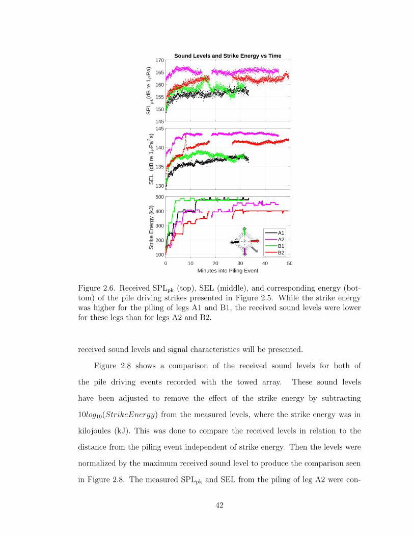
145
150
155
160
165
170
SP
Lp
k(dB
re
1P
a)
Sound Levels and Strike Energy vs Time
130
135
140
145
SE
L (
dB r
e 1
Pa
2s)
0 10 20 30 40 50
Minutes into Piling Event
100
200
300
400
500
Str
ike
Ene
rgy
(kJ)
A1A2B1B2
Figure 2.6. Received SPLpk (top), SEL (middle), and corresponding energy (bot-tom) of the pile driving strikes presented in Figure 2.5. While the strike energywas higher for the piling of legs A1 and B1, the received sound levels were lowerfor these legs than for legs A2 and B2.
received sound levels and signal characteristics will be presented.
Figure 2.8 shows a comparison of the received sound levels for both of
the pile driving events recorded with the towed array. These sound levels
have been adjusted to remove the effect of the strike energy by subtracting
10log10(StrikeEnergy) from the measured levels, where the strike energy was in
kilojoules (kJ). This was done to compare the received levels in relation to the
distance from the piling event independent of strike energy. Then the levels were
normalized by the maximum received sound level to produce the comparison seen
in Figure 2.8. The measured SPLpk and SEL from the piling of leg A2 were con-
42

0 100 200 300 400 500 600 700
Strike Energy (kJ)
125
130
135
140
145
150
SE
L (d
B r
e 1
Pa
2s)
SEL vs Strike Energy
A1A2B1B2
Figure 2.7. SEL versus strike energy for each recorded hammer strike from all 16measured piling events. The received levels for the piling of legs A2 and B2 wereconsistently higher than those for legs A1 and B1, independent of strike energy.This supports the determination that the dominant factor influencing the receivedsound levels from different legs is the inclination of the pile to the receiver.
sistently higher than that of leg A1 over the entire towed array transect, which is
thought to be due to the orientation of the leg relative to the receiver.
2.3.3 Variations in Signal Characteristics
The rise and decay time of the signal recorded on the towed array from each
hammer strike was calculated and plotted versus distance to investigate its de-
pendence on range from the foundation (Figure 2.9). Only signals with a high
enough signal-to-noise ratio to allow for reliable calculation of the rise time were
included in the following comparisons. The signals from the A1 leg had longer
rise and decay times over range than those from the A2 leg. These differences are
thought to be a function of the pile inclination relative to the towed array. Greater
seafloor interaction of the sound radiated from the A1 leg resulted in greater time
dispersion in the received signal.
Independent of the orientation of the pile, the rise and decay times and the
pulse duration of the signals recorded from both legs increased with range as
43

-30
-25
-20
-15
-10
-5
0
Norm
aliz
ed S
PL
pk (
dB
)
Normalized Sound Level vs Distance
A1
A2
0 1 2 3 4 5
Distance of Array from WTG (km)
-25
-20
-15
-10
-5
0
Norm
aliz
ed S
EL (
dB
)
Figure 2.8. Normalized SPLpk (top) and SEL (bottom) versus distance for eachhammer strike measured on the towed array for the pile driving of the A2 and A1legs. Levels have been adjusted to remove the effect of strike energy and normalizedto highlight the difference in received levels between the two piling events. Thedifference increases to around 10 dB by 5 km.
measured by the towed array. The energy in the pulse spreads over time as the
signal propagates further in range. These dispersion effects are expected when a
broadband acoustic signal is propagated in a shallow water environment (Potty
et al., 2003, 2000). Bailey et al. (2010) noted the same trend where there was a
decrease in sound level and an increase in pulse duration with increasing distance
from the piling.
The pulse duration for each of the signals represented in Figure 2.9 was plotted
versus the measured SEL (bottom plot in Figure 2.10). The signals were consis-
tently more spread in time for the piling of leg A1 than for leg A2 based on the
propagation paths of the radiated energy. This relationship supports the trend
44
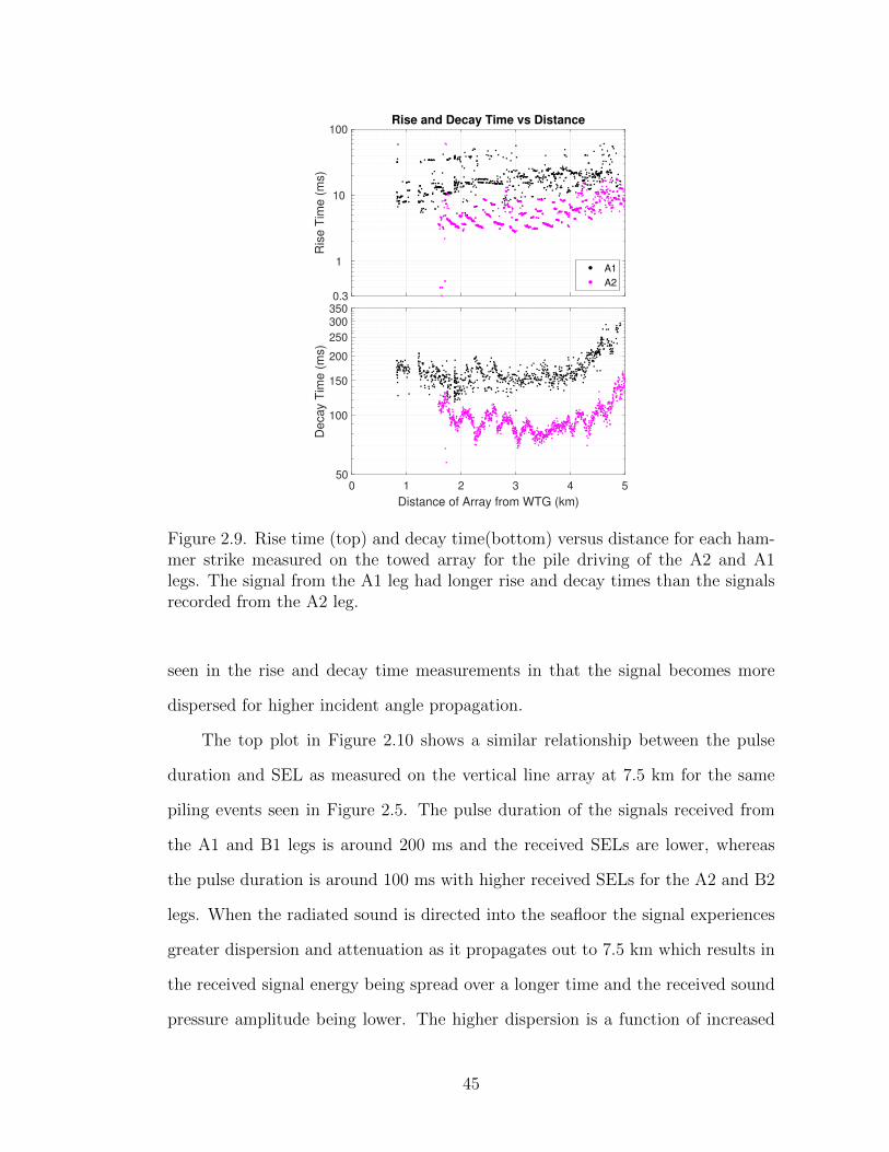
0.3
1
10
100
Ris
e T
ime
(m
s)
Rise and Decay Time vs Distance
A1
A2
0 1 2 3 4 5
Distance of Array from WTG (km)
50
100
150
200
250
300350
De
ca
y T
ime
(m
s)
Figure 2.9. Rise time (top) and decay time(bottom) versus distance for each ham-mer strike measured on the towed array for the pile driving of the A2 and A1legs. The signal from the A1 leg had longer rise and decay times than the signalsrecorded from the A2 leg.
seen in the rise and decay time measurements in that the signal becomes more
dispersed for higher incident angle propagation.
The top plot in Figure 2.10 shows a similar relationship between the pulse
duration and SEL as measured on the vertical line array at 7.5 km for the same
piling events seen in Figure 2.5. The pulse duration of the signals received from
the A1 and B1 legs is around 200 ms and the received SELs are lower, whereas
the pulse duration is around 100 ms with higher received SELs for the A2 and B2
legs. When the radiated sound is directed into the seafloor the signal experiences
greater dispersion and attenuation as it propagates out to 7.5 km which results in
the received signal energy being spread over a longer time and the received sound
pressure amplitude being lower. The higher dispersion is a function of increased
45
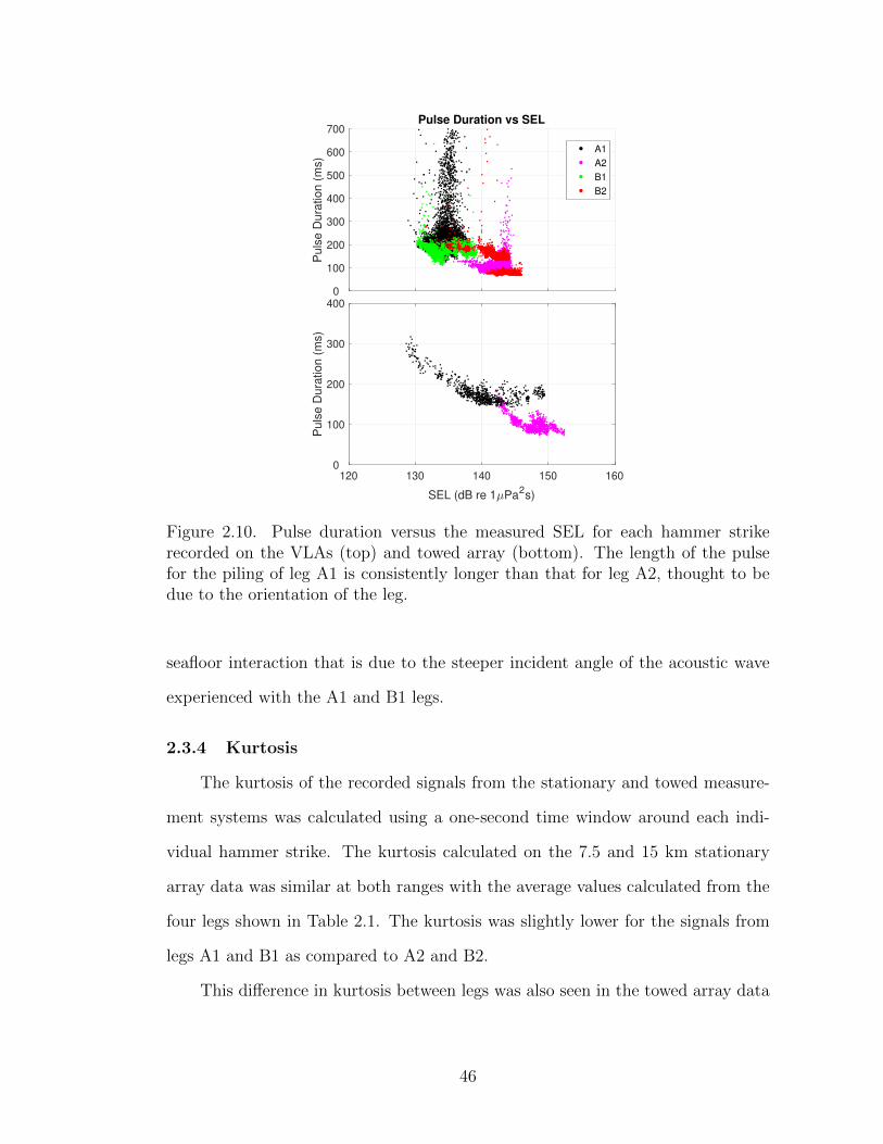
0
100
200
300
400
500
600
700
Pu
lse D
ura
tion
(m
s)
Pulse Duration vs SEL
A1
A2
B1
B2
120 130 140 150 160
SEL (dB re 1 Pa2s)
0
100
200
300
400
Puls
e D
ura
tion
(m
s)
Figure 2.10. Pulse duration versus the measured SEL for each hammer strikerecorded on the VLAs (top) and towed array (bottom). The length of the pulsefor the piling of leg A1 is consistently longer than that for leg A2, thought to bedue to the orientation of the leg.
seafloor interaction that is due to the steeper incident angle of the acoustic wave
experienced with the A1 and B1 legs.
2.3.4 Kurtosis
The kurtosis of the recorded signals from the stationary and towed measure-
ment systems was calculated using a one-second time window around each indi-
vidual hammer strike. The kurtosis calculated on the 7.5 and 15 km stationary
array data was similar at both ranges with the average values calculated from the
four legs shown in Table 2.1. The kurtosis was slightly lower for the signals from
legs A1 and B1 as compared to A2 and B2.
This difference in kurtosis between legs was also seen in the towed array data
46

shown in Figure 2.11. The higher kurtosis for the A2 leg, in combination with the
higher received sound levels and shorter pulse duration, implies that the signals
from this leg were more impulsive as compared to those from leg A1. All of these
factors can be related to the inclination of the pile relative to the receiver, where
the A2 leg oriented away from the receiver experiences less bottom interaction and
time dispersion in the propagated signal. The seafloor interaction is greater for
the A1 leg and results in a signal with a lower kurtosis and received sound level
and a longer pulse duration, which would describe a less impulsive signal.
Table 2.1. Average kurtosis calculated from the hammer strikes related to thepiling of each leg recorded on a single channel from the 7.5 and 15 km stationaryarrays.
Foundation Leg Kurtosis at 7.5 km Kurtosis at 15 kmA1 21.7 20.7A2 35.6 34.1B1 23.9 22.3B2 31.8 26.3
The goal of this analysis was to use kurtosis to characterize the impulsiveness
of the signal and determine if there was a range at which the signal could be
classified as non-impulsive based on this metric. No clear transition range or
threshold were seen in the data presented in Figure 2.11. In order to define a
range at which the signal transitions, a threshold would need to be defined below
which a signal could be considered non-impulsive. Without a clear threshold to
compare against, the measurements in Figure 2.11 show that the signals from leg
A2 have higher kurtosis and could be considered more impulsive relative to the
signals received from leg A1 over the same range.
47
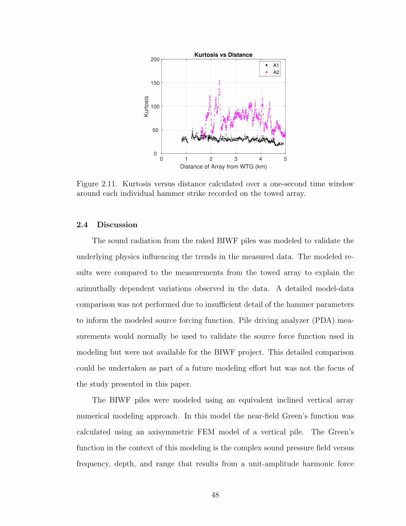
0 1 2 3 4 5
Distance of Array from WTG (km)
0
50
100
150
200
Kurt
osis
Kurtosis vs Distance
A1
A2
Figure 2.11. Kurtosis versus distance calculated over a one-second time windowaround each individual hammer strike recorded on the towed array.
2.4 Discussion
The sound radiation from the raked BIWF piles was modeled to validate the
underlying physics influencing the trends in the measured data. The modeled re-
sults were compared to the measurements from the towed array to explain the
azimuthally dependent variations observed in the data. A detailed model-data
comparison was not performed due to insufficient detail of the hammer parameters
to inform the modeled source forcing function. Pile driving analyzer (PDA) mea-
surements would normally be used to validate the source force function used in
modeling but were not available for the BIWF project. This detailed comparison
could be undertaken as part of a future modeling effort but was not the focus of
the study presented in this paper.
The BIWF piles were modeled using an equivalent inclined vertical array
numerical modeling approach. In this model the near-field Green’s function was
calculated using an axisymmetric FEM model of a vertical pile. The Green’s
function in the context of this modeling is the complex sound pressure field versus
frequency, depth, and range that results from a unit-amplitude harmonic force
48
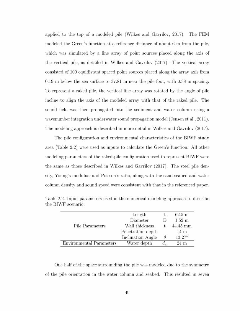
applied to the top of a modeled pile (Wilkes and Gavrilov, 2017). The FEM
modeled the Green’s function at a reference distance of about 6 m from the pile,
which was simulated by a line array of point sources placed along the axis of
the vertical pile, as detailed in Wilkes and Gavrilov (2017). The vertical array
consisted of 100 equidistant spaced point sources placed along the array axis from
0.19 m below the sea surface to 37.81 m near the pile foot, with 0.38 m spacing.
To represent a raked pile, the vertical line array was rotated by the angle of pile
incline to align the axis of the modeled array with that of the raked pile. The
sound field was then propagated into the sediment and water column using a
wavenumber integration underwater sound propagation model (Jensen et al., 2011).
The modeling approach is described in more detail in Wilkes and Gavrilov (2017).
The pile configuration and environmental characteristics of the BIWF study
area (Table 2.2) were used as inputs to calculate the Green’s function. All other
modeling parameters of the raked-pile configuration used to represent BIWF were
the same as those described in Wilkes and Gavrilov (2017). The steel pile den-
sity, Young’s modulus, and Poisson’s ratio, along with the sand seabed and water
column density and sound speed were consistent with that in the referenced paper.
Table 2.2. Input parameters used in the numerical modeling approach to describethe BIWF scenario.
Pile Parameters
Length L 62.5 mDiameter D 1.52 m
Wall thickness t 44.45 mmPenetration depth 14 mInclination Angle θ 13.27◦
Environmental Parameters Water depth dw 24 m
One half of the space surrounding the pile was modeled due to the symmetry
of the pile orientation in the water column and seabed. This resulted in seven
49
azimuth angles between 0◦ and 180◦ being modeled in 30◦ increments. The model
was computed on a frequency grid from 10 Hz to 2000 Hz in 1 Hz increments to
encompass the frequency bands with the majority of the sound energy measured
from BIWF. The coupling range of the sound field model to be propagated to
longer ranges from the inclined vertical array was 20 m.
The Green’s function of the raked pile in the underwater sound channel was
calculated at a range of 20 m, for 200 receiver depths ranging between 0.38 m to 76
m at increments of 0.38 m, and for seven azimuths. The modeled azimuth of 30◦
is in the direction of pile incline where the radiated sound is directed towards the
seafloor (as measured with leg A1) as opposed to the azimuth of 150◦ which is in the
direction opposite the pile incline where the radiated sound is directed through the
water column (as measured with leg A2). The magnitude of the Green’s functions
calculated at a range of 20 m for azimuths of 30◦ and 150◦ is shown in Figure 2.12.
The differences between the sound radiated along each azimuth are highlighted in
the figure. The magnitude of the radiated sound is greater near the seafloor along
the 30◦ azimuth as compared to the 150◦ azimuth.
The combined effect that the depth, frequency, and azimuth dependent differ-
ences have on the propagation of the pile driving signal over range was investigated
by utilizing the ORCA normal mode model (Westwood et al., 1996). This algo-
rithm was used to propagate the Green’s function estimated at 20 m out to a
range of 3 km. The modeled SEL was similar along the two azimuths out to
a range of around 300 m, after which the SEL along the 150◦ azimuth (radiated
sound directed through water column) was greater than that along the 30◦ azimuth
(radiated sound directed at seafloor) (Figure 2.13).
The modeled sound fields were compared to the measurements from the towed
array to validate the fall-off and azimuthal discrepancies observed in the data. The
50

Figure 2.12. Modeled Green’s function (GF) magnitude at 20 m range from theraked pile at azimuths of 30◦ (top) and 150◦ (bottom) to correspond to the az-imuths of the towed array transects during the leg A1 and A2 pile driving events,respectively. The line at a depth of 24 meters represents the modeled seafloor.
measured data were adjusted to remove the effect of strike energy as described in
Section III.B. Modeled SEL at azimuths of 30◦ and 150◦ at a depth of 12 m,
which corresponds to the depth of the towed array, were compared to the adjusted
measured SEL during the piling events. The modeled and adjusted measured
values were normalized to highlight the differences in levels along the two azimuths
(Figure 2.13).
The model results predict azimuthal differences in the resulting sound field
from the piling of a raked pile. These differences increase to more than 10 dB as
the range increases due to the vertical directionality of the sound source at different
azimuth angles. A detailed comparison of the model results to the measured levels
will be undertaken as a further study.
51

0.02 0.05 0.1 0.2 0.5 1 2 3 4 5
Range (km)
-50
-40
-30
-20
-10
0
No
rma
lize
d S
EL
Diffe
ren
ce
(d
B)
Normalized SEL Comparison
30o
150o
A1
A2
Figure 2.13. Comparison between the measured data (adjusted for strike energyand normalized) on the towed array and the normalized modeled data along the30◦ and 150◦ azimuths. Differences in SEL of approximately 10 dB are observedat a range of 3 km.
2.5 Conclusions
The dominant factor influencing the received sound levels from the installa-
tion of raked piles via impact pile driving was the inclination of the pile being
driven relative to the receiver. The jacket foundation at BIWF required piles to
be driven on an angle of 13.27◦ and the received sound levels and measured signal
characteristics exhibited azimuthal dependence. The rake of the pile directed the
radiated sound towards the seafloor in the direction of the pile incline (as with
legs A1 and B1) and near horizontally in the direction opposite the pile incline (as
with legs A2 and B2). The azimuthal discrepancy observed in the measurements
collected at BIWF was due to the raked piles in the foundation.
Sound levels differences of 5-10 dB were observed for piles inclined in opposite
directions. The magnitude and trend of the azimuthal discrepancies in sound level
were explained with the model results. More detailed modeling and comparison to
measured results will be a focus of further study.
The kurtosis demonstrated that the signals received along azimuths in the
52
direction of pile incline were less impulsive than the signals received along the
azimuths opposite the pile incline. This was consistent with the rise and decay
time and pulse duration of the signals being longer when the energy was radiated
more towards the seafloor as opposed to through the water column. The kurtosis
decreased, while the rise time, decay time, and pulse duration increased, with range
from the piling activity as the signal became more dispersed and less impulsive.
Additional analysis is needed to determine which metrics and thresholds most
reliably describe when a signal transitions from being considered impulsive to non-
impulsive. This information would be beneficial when assessing sound exposure on
marine animals and determining the best exposure criteria to use.
The azimuthal variability in the sound field is an important factor to consider
for noise mitigation and environmental assessments that are performed for raked
pile installations. Environmental assessments determine the range to different
acoustic thresholds enforced by federal regulations. The azimuthally dependent
sound fields from a raked pile installation will impact those ranges. This will result
in the mitigation range being larger along azimuths closer to 180◦ as opposed to
those along azimuths closer to 0◦ measured along the pile axis relative to a receiver.
Acknowledgments: This paper was presented at the fifth International
Meeting on The Effects of Noise on Aquatic Life held in Den Haag, July
2019. Study concept, oversight, and funding for the experiment were provided
by the U.S. Department of the Interior, Bureau of Ocean Energy Management
(BOEM), Environmental Studies Program, Washington, DC under Contract Num-
ber M15PC00002, Task Order M16PD00025. Collaborators in this project include
Randy Gallien and Anwar Khan (HDR, Inc.).
53
Bibliography
Bailey, H., Senior, B., Simmons, D., Rusin, J., Picken, G., and Thompson, P. M.
(2010). Assessing underwater noise levels during pile-driving at an offshore wind-
farm and its potential effects on marine mammals. Marine Pollution Bulletin,
60(6):888–897.
Dahl, P. H. and Dall’Osto, D. R. (2017). On the underwater sound field from
impact pile driving: Arrival structure, precursor arrivals, and energy streamlines.
The Journal of the Acoustical Society of America, 142(2):1141–1155.
Dahl, P. H. and Reinhall, P. G. (2013). Beam forming of the underwater sound
field from impact pile driving. The Journal of the Acoustical Society of America,
134(1).
De Jong, C. and Ainslie, M. A. (2008). Underwater radiated noise due to the
piling for the Q7 Offshore Wind Park. In The Journal of the Acoustical Society
of America, volume 123.
Erdreich, J. (1986). A distribution based definition of impulse noise. Journal of
the Acoustical Society of America, 79(4):990–998.
Gottsche, K. M., Steinhagen, U., and Juhl, P. M. (2015). Numerical evaluation of
pile vibration and noise emission during offshore pile driving. Applied Acoustics,
99:51–59.
Hamernik, R. P., Qiu, W., and Davis, B. (2003). The effects of the amplitude dis-
tribution of equal energy exposures on noise-induced hearing loss: The kurtosis
metric. The Journal of the Acoustical Society of America, 114(1):386–395.
54
Hastie, G., Merchant, N. D., Gotz, T., Russell, D. J. F., Thompson, P., and Janik,
V. M. (2019). Effects of impulsive noise on marine mammals: investigating range
dependent risk. Ecological Applications.
HDR (2018). Field Observations During Wind Turbine Foundation Installation
at the Block Island Wind Farm, Rhode Island Appendix D: Underwater Sound
Monitoring Reports.
Henderson, D. and Hamernik, R. P. (1986). Impulse Noise: Critical Review. Jour-
nal of the Acoustical Society of America, 80(2):569–584.
ISO (1997). ISO 10843 Acoustics - Methods for the description and physical mea-
surement of single impulses or series of impulses. International Organization for
Standardization, Geneva, Switzerland.
ISO (2017a). ISO 18405 Underwater Acoustics - Terminology. International Or-
ganization for Standardization, Geneva, Switzerland.
ISO (2017b). ISO 18406 Underwater acoustics a¿” Measurement of radiated un-
derwater sound from percussive pile driving. International Organization for Stan-
dardization, Geneva, Switzerland.
Jensen, F. B., Kuperman, W. A., Porter, M. B., and Schmidt, H. (2011). Compu-
tational Ocean Acoustics. Springer Science, New York, NY, second edition.
Kastelein, R. A., Helder-Hoek, L., Van de Voorde, S., von Benda-Beckmann, A. M.,
Lam, F.-P. A., Jansen, E., de Jong, C. A. F., and Ainslie, M. A. (2017). Tem-
porary hearing threshold shift in a harbor porpoise ( Phocoena phocoena ) after
exposure to multiple airgun sounds. The Journal of the Acoustical Society of
America, 142(4):2430–2442.
55
Kim, H., Miller, J. H., and Potty, G. R. (2013). Predicting underwater radiated
noise levels due to the first offshore wind turbine installation in the U.S. Pro-
ceedings of Meetings on Acoustics, 19:040067.
Laughlin, J. (2005). Underwater Sound Levels Associated With Pile Driving on
the Sr 24 , I-82 To Keys Road Project a¿“ Yakima River. Technical Report
July, Washington State Department of Transportation.
Lei, S., Ahroon, W. A., and Hamernik, R. P. (1994). The application of frequency
and time domain kurtosis to the assessment of hazardous noise exposures. The
Journal of the Acoustical Society of America, 95(5):3005–3005.
Lin, Y.-T., Newhall, A. E., Miller, J. H., Potty, G. R., and Vigness-Raposa, K. J.
(2019). A three-dimensional underwater sound propagation model for offshore
wind farm noise prediction. The Journal of the Acoustical Society of America,
145(5):EL335–EL340.
MacGillivray, A. (2018). Underwater noise from pile driving of conductor casing
at a deep-water oil platform. The Journal of the Acoustical Society of America,
143(1):450–459.
Martin, S. B. (2019). One minute at a time: Advancing our ability to estimate
effects of man-made sound on marine life. PhD thesis, Dalhousie University
Halifax, Nova Scotia.
Martin, S. B. and Barclay, D. R. (2019). Determining the dependence of marine
pile driving sound levels on strike energy , pile penetration , and propagation
effects using a linear mixed model based on damped cylindrical spreading. The
Journal of the Acoustical Society of America, 146(1):109–121.
56

National Marine Fisheries Service (2018). 2018 Revision to: Technical Guidance
for Assessing the Effects of Anthropogenic Sound on Marine Mammal Hearing
(Version 2.0): Underwater Thresholds for Onset of Permanent and Temporary
Threshold Shifts. Technical report, U.S. Department of Commerce, NOAA.
National Marine Fisheries Service (NMFS) (2015). DRAFT Guidance for Assessing
the Effects of Anthropogenic Sound on Marine Mammal Hearing. Technical
report, U.S. Department of Commerce.
Norro, A. M. J., Rumes, B., and Degraer, S. J. (2013). Differentiating between
Underwater Construction Noise of Monopile and Jacket Foundations for Offshore
Windmills: A Case Study from the Belgian Part of the North Sea. The Scientific
World Journal, pages 1–7.
Popper, A. N., Carlson, T. J., Hawkins, A. D., Southall, B. L., and Gentry, R. L.
(2006). Interim Criteria for Injury of Fish Exposed to Pile Driving Operations
: A White Paper.
Popper, A. N., Hawkins, A. D., Fay, R. R., Mann, D. A., Bartol, S., Carlson,
T. J., Coombs, S., Ellison, W. T., Gentry, R. L., Halvorsen, M. B., Løkkeborg, S.,
Rogers, P. H., Southall, B. L., Zeddies, D. G., and Tavolga, W. N. (2014). Sound
Exposure Guidelines for Fishes and Sea Turtles: A Technical Report prepared by
ANSI-Accredited Standards Committee S3/SC1 and registered with ANSI. ASA
S3/SC1.4 TR-2014. Springer International Publishing, Cham, Switzerland.
Potty, G. R., Miller, J. H., and Lynch, J. F. (2003). Inversion for sediment geoa-
coustic properties at the New England Bight. The Journal of the Acoustical
Society of America, 114(4):1874–1887.
Potty, G. R., Miller, J. H., Lynch, J. F., and Smith, K. B. (2000). Tomographic
57

inversion for sediment parameters in shallow water. The Journal of the Acoustical
Society of America, 108(3):973–986.
Reinhall, P. G. and Dahl, P. H. (2011). Underwater Mach wave radiation from
impact pile driving: Theory and observation. The Journal of the Acoustical
Society of America, 130(3):1209–1216.
Robinson, S. P., Theobald, P. D., and Lepper, P. A. (2012). Underwater noise
generated from marine piling. Proceedings of Meetings on Acoustics, 17.
Southall, B. L., Bowles, A. E., Ellison, W. T., Finneran, J. J., Gentry, R. L., Greene
Jr, C. R., Kastak, D., Ketten, D. R., Miller, J. H., Nachtigall, P. E., Richardson,
W. J., Tomas, J. A., and Tyack, P. L. (2007). Marine Mammal Noise Exposure
Criteria: Initial Scientific Recommendations. Aquatic Mammals, 33(4).
Southall, B. L., Finneran, J. J., Reichmuth, C., Nachtigall, P. E., Ketten, D. R.,
Bowles, A. E., Ellison, W. T., Nowacek, D. P., and Tyack, P. L. (2019). Ma-
rine Mammal Noise Exposure Criteria: Updated Scientific Recommendations
for Residual Hearing Effects. Aquatic Mammals, 45(2):125–232.
Tetra Tech (2012). Block Island Wind Farm and Block Island Transmission System
Environmental Report / Construction and Operations Plan. Technical report,
Submitted by Deepwater Wind, Boston, MA.
Tetra Tech and JASCO (2015). Hydroacoustic Monitoring Program Final Tech-
nical Report Block Island Wind Farm Construction 2015. Technical report,
Prepared for Deepwater Wind Block Island, LLC.
Westwood, E. K., Tindle, C. T., and Chapman, N. R. (1996). A normal mode
model for acousto-elastic ocean environments. The Journal of the Acoustical
Society of America, 100(6):3631–3645.
58
Wilkes, D. R. and Gavrilov, A. N. (2017). Sound radiation from impact-driven
raked piles. Journal of the Acoustical Society of America, 142(1):1–11.
Zampolli, M., Nijhof, M. J. J., de Jong, C. A. F., Ainslie, M. A., Jansen, E. H. W.,
and Quesson, B. A. J. (2013). Validation of finite element computations for
the quantitative prediction of underwater noise from impact pile driving. The
Journal of the Acoustical Society of America, 133(1):72–81.
59

MANUSCRIPT 3
Fin whale localization and environmental inversion using modalarrivals of the 20-Hz pulse
This manuscript is currently unpublished.
Jennifer L. Amaral, James H. Miller and Gopu R. Potty
Department of Ocean Engineering, University of Rhode Island, Narragansett, RI
02882, USA
Ying-Tsong Lin
Applied Ocean Physics and Engineering, Woods Hole Oceanographic Institution,
Woods Hole, MA 02543, USA
Kathleen Vigness-Raposa
INSPIRE Environmental, 513 Broadway, Suite 314, Newport, RI 02840, USA
60
Abstract: Fin whale doublet calls, described as two 20-Hz pulses recorded at
different interpulse intervals, have been attributed to the whale’s calling behavior,
however they could also result from acoustic mode propagation effects. Modes
travel with their own frequency-dependent group velocities. The dispersion of
these modes results in the sound being recorded as multiple arrivals on a receiver.
Multiple modal arrivals of 20-Hz fin whale calls were recorded, with mode one ar-
riving after mode two. The time delay between modal arrivals varied throughout
the recording and is range dependent. The range dependency of this time delay
was used to estimate the range of the whale from individual hydrophones by de-
termining the modal group velocities that resulted in the observed delays. A pair
of hydrophones was used to localize the whale for the duration of time when two
modes were detected. The KRAKEN normal mode model was utilized in an inver-
sion scheme to determine the compressional wave speed and depth to bedrock in
the study area that supported the estimated modal group velocities. The inversion
resulted in a depth to bedrock of 205 m and compressional wave speed of 1735 m/s,
which were supported by measurements reported in literature for nearby regions.
[Work supported by BOEM]
61
3.1 Introduction
Fin whales (Balaenoptera physalus) produce stereotyped low frequency songs
that are composed of a series of 20-Hz pulses that repeat at consistent time in-
tervals for long durations and have been recorded worldwide (Sirovic et al., 2007;
Rebull et al., 2006; Weirathmueller et al., 2017; Thompson et al., 1992; Castellote
et al., 2012; Miksis-Olds et al., 2019). The 20-Hz pulse is a high-amplitude and
short-duration chirp lasting less than 1 second that sweeps down in frequency be-
tween approximately 23 to 18 Hz (Watkins et al., 1987). A sequence of regularly
occuring 20-Hz pulses is known as a song and a sequence of songs is known as
a song bout (Clark et al., 2019). Individual fin whale songs within a bout are
separated from each other by silent periods that occur at approximtely 15 minute
intervals (Watkins et al., 1987). Within a song, consecutive 20-Hz pulses occur at
consistent time intervals, which is referred to as the interpulse interval, and is the
time between successive pulses measured from a point on one pulse to the same
point on a succeeding pulse (Thompson et al., 1992).
The composition of recorded fin whale song has been described as 20-Hz pulses
repeating at regularly repeated pulse intervals, either at one nominal pulse rate
(singlet) or at two alternating pulse intervals (doublet) (Thompson et al., 1992;
Watkins et al., 1987). This doublet phenomenon has been attributed to the fin
whale’s calling behavior, but additional observations have been made that suggest
the 20-Hz doublet pattern could be explained by multipath arrivals of a single
20-Hz pulse at the acoustic instrument rather than the fin whale emitting two
pulses at alternating interpulse intervals (Premus and Spiesberger, 1997). If the
doublet pattern is an artifact of propagation, then information contained within
the recorded signal could be used for passive ranging and localization of the whale
and geoacoustic inversions to estimate environmental parameters (Premus and
62
Spiesberger, 1997; Kuna and Nabelek, 2021).
Multipath propagation in shallow water environments can be described by
normal mode theory. A normal mode is described as a standing wave between the
boundaries of an acoustic waveguide that propagates horizontally with a frequency-
dependent group speed (Jensen et al., 2011). The number of propagating modes
depends on the depth of the waveguide and frequency of the source. As a pulse
propagates down a waveguide, the individual modes will travel at independent
group velocities and arrive at a receiver at different times, known as modal disper-
sion.
In shallow water waveguides, recorded calls from whales at ranges of more than
several water depths may become distorted due to multimode dispersion (Wiggins
et al., 2004; Lin et al., 2012). Premus and Spiesberger (1997) discussed that the
time delay between modal arrivals is strongly range dependent and can be used, in
conjunction with geoacoustic knowledge of the environment, to estimate the range
of the whale using only a single hydrophone. Additionally, passive localization can
be achieved using only a pair of hydrophones. While the range estimate is insen-
sitive to the depth of the whale, the ranging can only be achieved when multiple
modes are detected. Detection of these modes is limited by the detection range
of the first arrival which is typically the water-borne pulse, but also could be the
sediment-refracted/basement-reflected path if the compressional wave speed in the
sediment layers is higher than that in the water column (Premus and Spiesberger,
1997).
The study presented in this paper focuses on the use of multipath arrivals of
20-Hz fin whale calls to localize a whale and invert for environmental properties
in a shallow water study area. Multiple arrays were deployed off the coast of
Block Island, Rhode Island, USA that recorded a fin whale of opportunity as it
63

vocalized for over eighteen hours in the vicinity of the sensors. Individual 20-Hz
pulses arrived at the receiver as two distinct modes and the time delay between
modal arrivals varied throughout the recording. The range dependency of this time
delay was exploited to estimate the range of the whale from individual sensors by
determining the modal group velocities that resulted in the observed time delays.
Once the range of the whale from individual hydrophones was found, a pair of
hydrophones was used to localize the whale for the duration of time when two
modes were detected in the recorded data. The KRAKEN normal mode model
was then used to invert for the sediment compressional wave speed and depth to
bedrock in the study area that supported the estimated modal group speeds.
The paper is organized in the following manner. Section II describes the study
location along with the measurement equipment. Section III presents the method
used to detect the fin whale calls in the dataset. Sections IV and V present the
fin whale and modal detections. Secton VI presents the method used to determine
the range difference of the whale from the deployed arrays. Section VII presents
the fin whale detections recorded on a different deployed sensor suite that was
used to validate the detections on the deployed arrays. Section VIII dicusses the
localization of the whale and Section VIIII presents the inversion method and
results. A discussion is presented in Section X, followed by the conclusions of the
study in Section XI.
3.2 Measurement Equipment
Two vertical line arrays (referred to as Array 1 and Array 2) were deployed
for 24 days between October and November 2015 off the coast of Block Island,
Rhode Island, USA (Figure 3.1). These sensor systems were deployed as part of
the Bureau of Ocean Energy Management (BOEM) funded Real-time Opportunity
for Development Environmental Observations (RODEO) program with the objec-
64
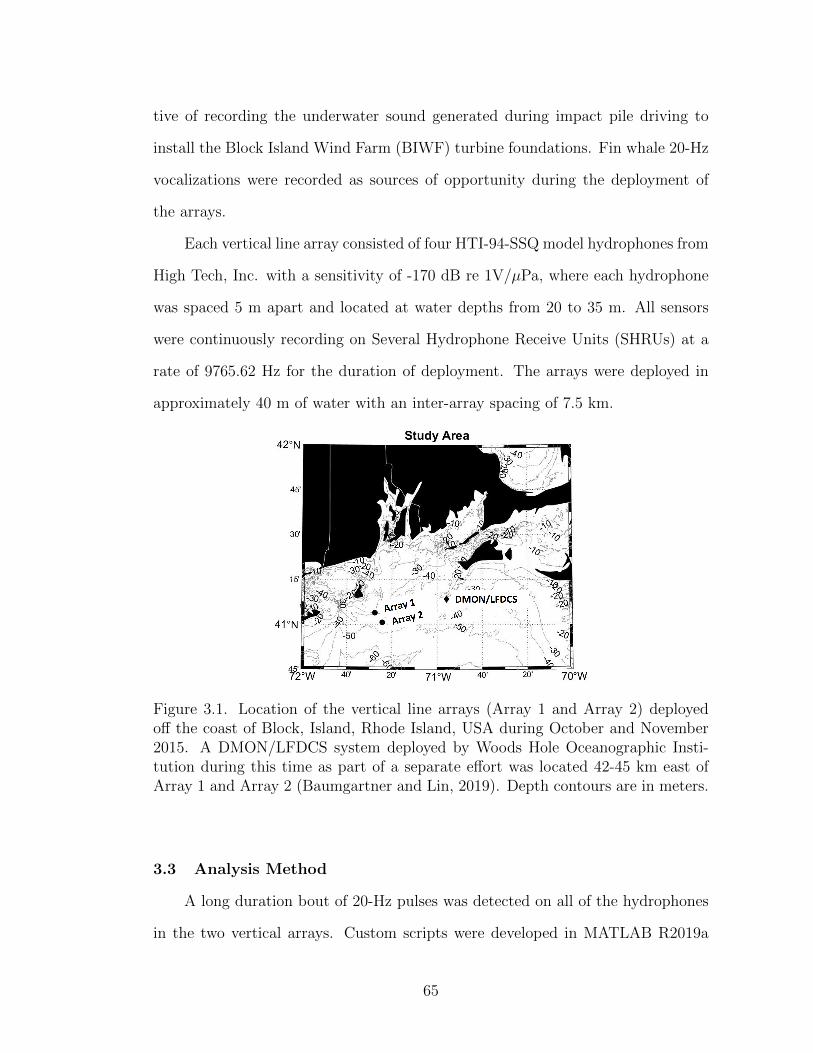
tive of recording the underwater sound generated during impact pile driving to
install the Block Island Wind Farm (BIWF) turbine foundations. Fin whale 20-Hz
vocalizations were recorded as sources of opportunity during the deployment of
the arrays.
Each vertical line array consisted of four HTI-94-SSQ model hydrophones from
High Tech, Inc. with a sensitivity of -170 dB re 1V/µPa, where each hydrophone
was spaced 5 m apart and located at water depths from 20 to 35 m. All sensors
were continuously recording on Several Hydrophone Receive Units (SHRUs) at a
rate of 9765.62 Hz for the duration of deployment. The arrays were deployed in
approximately 40 m of water with an inter-array spacing of 7.5 km.
Figure 3.1. Location of the vertical line arrays (Array 1 and Array 2) deployedoff the coast of Block, Island, Rhode Island, USA during October and November2015. A DMON/LFDCS system deployed by Woods Hole Oceanographic Insti-tution during this time as part of a separate effort was located 42-45 km east ofArray 1 and Array 2 (Baumgartner and Lin, 2019). Depth contours are in meters.
3.3 Analysis Method
A long duration bout of 20-Hz pulses was detected on all of the hydrophones
in the two vertical arrays. Custom scripts were developed in MATLAB R2019a
65

(www.mathworks.com) to detect and analyze the recorded 20-Hz pulses for the
entire duration of the recording. The acoustic recordings were decimated to a
sampling rate of approximately 1 kHz to allow for more efficient processing and
analysis. Data were then band pass filtered (fifth-order Chebyshev type II) between
10-30 Hz prior to detecting the pulses. The data from a single sensor on either
array were utilized for the analysis presented in this paper. The sensors located at
a depth of 25 m on Array 1 and at a depth of 26 m on Array 2 were used for further
analysis because they had the highest received levels on each array. A segment of
data showing three individual songs within the recorded bout is shown in Figure
3.2.
Figure 3.2. Time series (top) and spectrogram (bottom) of a segment of the finwhale bout recorded on a single hydrophone in Array 2 (hydrophone at 26 m depth)showing three individual songs. Data has been bandpass filtered to improve SNRof the 20-Hz pulses. Time axis is UTC.
66

3.4 Modal Detections
Two distinct modal arrivals of individual 20-Hz pulses were observed in the
data recorded on the arrays (Figure 3.3) and scripts were written to detect and
analyze each modal arrival separately. Higher mode numbers traditionally corre-
spond to higher grazing angles and therefore higher modes would penetrate deeper
into seafloor at the frequencies of interest to this paper. If the compressional wave
speed in the sediment is higher than the sound speed through the water column
then the sediment-refracted/basement-reflected path could arrive first. The waveg-
uide in this study area is thought to encompass the sediment/subfloor layers in
addition to the water column and the compressional wave speed in the sediment
is higher than that in the water column, therefore the sediment-dominated mode
is estimated to arrive first.
The mode one arrival of the 20-Hz pulse was detected by cross correlating the
time series with a representative 20-Hz pulse. The representative pulse used was
selected from the data as a pulse that had a high signal-to-noise ratio and only
one modal arrival. Correlations above a threshold were classified as detections
and saved for further analysis. All detections were manually verified and false
detections were disregarded.
The mode two arrival was lower in both amplitude and bandwidth than the
mode one arrival and arrived before the mode one arrival (Figure 3.3). The mode
two arrivals were detected by finding peaks in the envelope of the time series
signal above a threshold that arrived before the largest amplitude detection. All
detections were manually verified and false detections were disregarded. The lower
amplitude modal arrivals that had a peak-signal to rms-noise ratio above 15 dB
were included in further analysis.
67
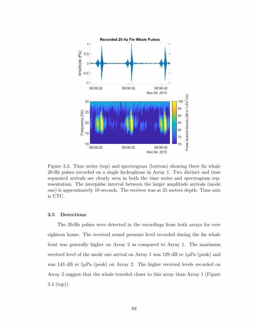
Figure 3.3. Time series (top) and spectrogram (bottom) showing three fin whale20-Hz pulses recorded on a single hydrophone in Array 1. Two distinct and timeseparated arrivals are clearly seen in both the time series and spectrogram rep-resentation. The interpulse interval between the larger amplitude arrivals (modeone) is approximately 10 seconds. The receiver was at 25 meters depth. Time axisis UTC.
3.5 Detections
The 20-Hz pulses were detected in the recordings from both arrays for over
eighteen hours. The received sound pressure level recorded during the fin whale
bout was generally higher on Array 2 as compared to Array 1. The maximum
received level of the mode one arrival on Array 1 was 129 dB re 1µPa (peak) and
was 143 dB re 1µPa (peak) on Array 2. The higher received levels recorded on
Array 2 suggest that the whale traveled closer to this array than Array 1 (Figure
3.4 (top)).
68

Figure 3.4. Comparison of the peak sound pressure levels (dB re 1µPa) from thelarger amplitude modal arrival measured on both arrays throughout the recordedbout (top). Difference in the path length of the fin whale signals received on asingle sensor in both arrays. A positive distance means the signal was received onArray 2 before Array 1 and a negative distance means the signal was received onArray 1 before Array 2 (bottom). The hydrophone used to generate these data isat a depth of 25 m on Array 1 and 26 m on Array 2. Time axis is UTC.
Long duration 20-Hz song bouts are thought to be breeding displays made by
male fin whales (Croll et al., 2002). The evidence supports the hypothesis that
these vocalizations were from one male fin whale because the bout was recorded at
the beginning of the reproductive season, which runs from November through May
(Morano et al., 2012), and there were no overlapping detections throughout this
song bout. Watkins (1981) also observed that these patterns of 20-Hz pulses were
mostly heard in the winter season and were produced by only one fin whale either
traveling in a group or separated from other fin whales by several kilometers.
69
Sequential pulses within a bout are relatively constant in level, but the pulses
immediately following or preceding a quiet period have been found to be of lower
level in recordings made in both the Atlantic (Watkins et al., 1987) and North
Pacific (Helble et al., 2020). This phenomenon was also observed in the recorded
signal bout. No explanation has been provided for these lower levels, but it has
been theorized that they could be due to lower source levels from the fin whale
or due to higher acoustic transmission loss when the whale is closer to the surface
(Helble et al., 2020), assuming the whale is surfacing during the rest periods.
3.6 Range Difference
The difference in arrival time of mode one on a single sensor in each array was
measured. This difference in arrival time was used to calculate the range difference
of the whale between the arrays (Figure 3.4 (bottom)). The maximum difference
in range is 7.5 km, which is the spacing between the two arrays. This maximum
difference in range would be expected when the whale’s position was directly in
line with the two arrays, which would imply the signal arrived on Array 2 first and
then traveled 7.5 km before reaching Array 1.
The received levels recorded on Array 2 were higher than those recorded on
Array 1 up through approximately 13:00, before the received levels became similar
on both arrays (Figure 3.4 (top)). This implies that the whale was closer to Array 2
up until this time and then the whale traversed a track that was a similar distance
from both arrays. This is confirmed by the variation in the range difference. As
the whale approaches the arrays, it is farther from Array 1 than it is from Array
2. The range difference between arrivals is maximum at 11:30, which coincides
with the time of the maximum received sound levels measured on Array 2. This is
the time of the closest point of approach of the whale to the arrays. As the whale
moves away from the arrays, it follows a path bringing it closer to Array 1. After
70
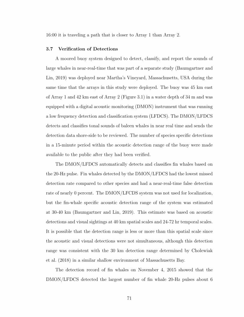
16:00 it is traveling a path that is closer to Array 1 than Array 2.
3.7 Verification of Detections
A moored buoy system designed to detect, classify, and report the sounds of
large whales in near-real-time that was part of a separate study (Baumgartner and
Lin, 2019) was deployed near Martha’s Vineyard, Massachusetts, USA during the
same time that the arrays in this study were deployed. The buoy was 45 km east
of Array 1 and 42 km east of Array 2 (Figure 3.1) in a water depth of 34 m and was
equipped with a digital acoustic monitoring (DMON) instrument that was running
a low frequency detection and classification system (LFDCS). The DMON/LFDCS
detects and classifies tonal sounds of baleen whales in near real time and sends the
detection data shore-side to be reviewed. The number of species specific detections
in a 15-minute period within the acoustic detection range of the buoy were made
available to the public after they had been verified.
The DMON/LFDCS automatically detects and classifies fin whales based on
the 20-Hz pulse. Fin whales detected by the DMON/LFDCS had the lowest missed
detection rate compared to other species and had a near-real-time false detection
rate of nearly 0 percent. The DMON/LFCDS system was not used for localization,
but the fin-whale specific acoustic detection range of the system was estimated
at 30-40 km (Baumgartner and Lin, 2019). This estimate was based on acoustic
detections and visual sightings at 40 km spatial scales and 24-72 hr temporal scales.
It is possible that the detection range is less or more than this spatial scale since
the acoustic and visual detections were not simultaneous, although this detection
range was consistent with the 30 km detection range determined by Cholewiak
et al. (2018) in a similar shallow environment of Massachusetts Bay.
The detection record of fin whales on November 4, 2015 showed that the
DMON/LFDCS detected the largest number of fin whale 20-Hz pulses about 6
71
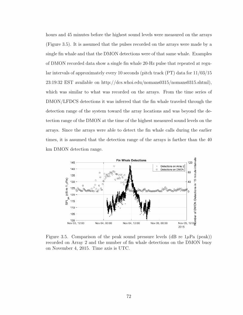
hours and 45 minutes before the highest sound levels were measured on the arrays
(Figure 3.5). It is assumed that the pulses recorded on the arrays were made by a
single fin whale and that the DMON detections were of that same whale. Examples
of DMON recorded data show a single fin whale 20-Hz pulse that repeated at regu-
lar intervals of approximately every 10 seconds (pitch track (PT) data for 11/03/15
23:19:32 EST available on http://dcs.whoi.edu/nomans0315/nomans0315.shtml),
which was similar to what was recorded on the arrays. From the time series of
DMON/LFDCS detections it was inferred that the fin whale traveled through the
detection range of the system toward the array locations and was beyond the de-
tection range of the DMON at the time of the highest measured sound levels on the
arrays. Since the arrays were able to detect the fin whale calls during the earlier
times, it is assumed that the detection range of the arrays is farther than the 40
km DMON detection range.
Figure 3.5. Comparison of the peak sound pressure levels (dB re 1µPa (peak))recorded on Array 2 and the number of fin whale detections on the DMON buoyon November 4, 2015. Time axis is UTC.
72

3.8 Localization Using Modal Arrivals
In normal mode theory, a signal measured on a receiver will be the summation
of all of the modes, however, individual modes traveling at different group velocities
will arrival at different times. The group velocity of a mode is the velocity at which
energy in the mode is transported. The number of propagating modes in a wave
guide is dependent on frequency and no sound can propagate at frequencies below
the cutoff frequency for the first mode, which is dependent on the depth of the
water, the sound speed in water, and the sound speed in the sediment (Urick,
1983).
Two distinct modal arrivals of the 20-Hz pulse were seen in the data collected
on the arrays. Multiple modes were not detectable prior to 07:00 or later than
15:30 in the dataset because the signal-to-noise ratio (SNR) of the higher order
modes was not greater then the ambient noise levels. The amplitude of mode one
was higher than the amplitude of mode two in the recorded data (Figure 3.6).
The time delay between the arrivals in the mode pairs from Figure 3.6 was
calculated. The time delay data was smoothed by taking the average time delay
in each song. The median song duration was 14 minutes long, so the average time
delay was taken every 14 minutes.
The time difference between the modal arrivals on a single hydrophone varied
throughout the recording (Figure 3.7) and was a function of the range of the whale
from the sensor. The time difference between arrivals was greater earlier in the
recording and decreased as the whale approached the array. Only one arrival
was identifiable in the data from Array 2 when the whale was closest to Array 2,
although two arrivals were seen in the data from Array 1 during this same time.
73
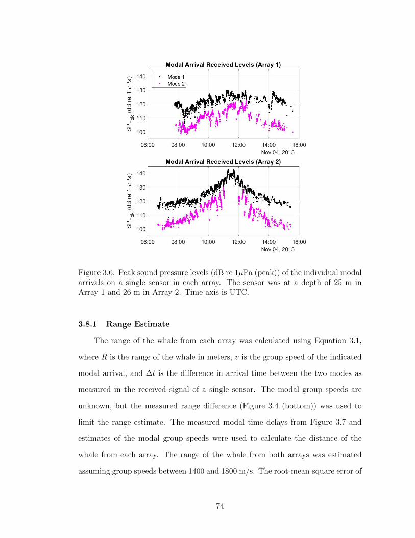
Figure 3.6. Peak sound pressure levels (dB re 1µPa (peak)) of the individual modalarrivals on a single sensor in each array. The sensor was at a depth of 25 m inArray 1 and 26 m in Array 2. Time axis is UTC.
3.8.1 Range Estimate
The range of the whale from each array was calculated using Equation 3.1,
where R is the range of the whale in meters, v is the group speed of the indicated
modal arrival, and ∆t is the difference in arrival time between the two modes as
measured in the received signal of a single sensor. The modal group speeds are
unknown, but the measured range difference (Figure 3.4 (bottom)) was used to
limit the range estimate. The measured modal time delays from Figure 3.7 and
estimates of the modal group speeds were used to calculate the distance of the
whale from each array. The range of the whale from both arrays was estimated
assuming group speeds between 1400 and 1800 m/s. The root-mean-square error of
74
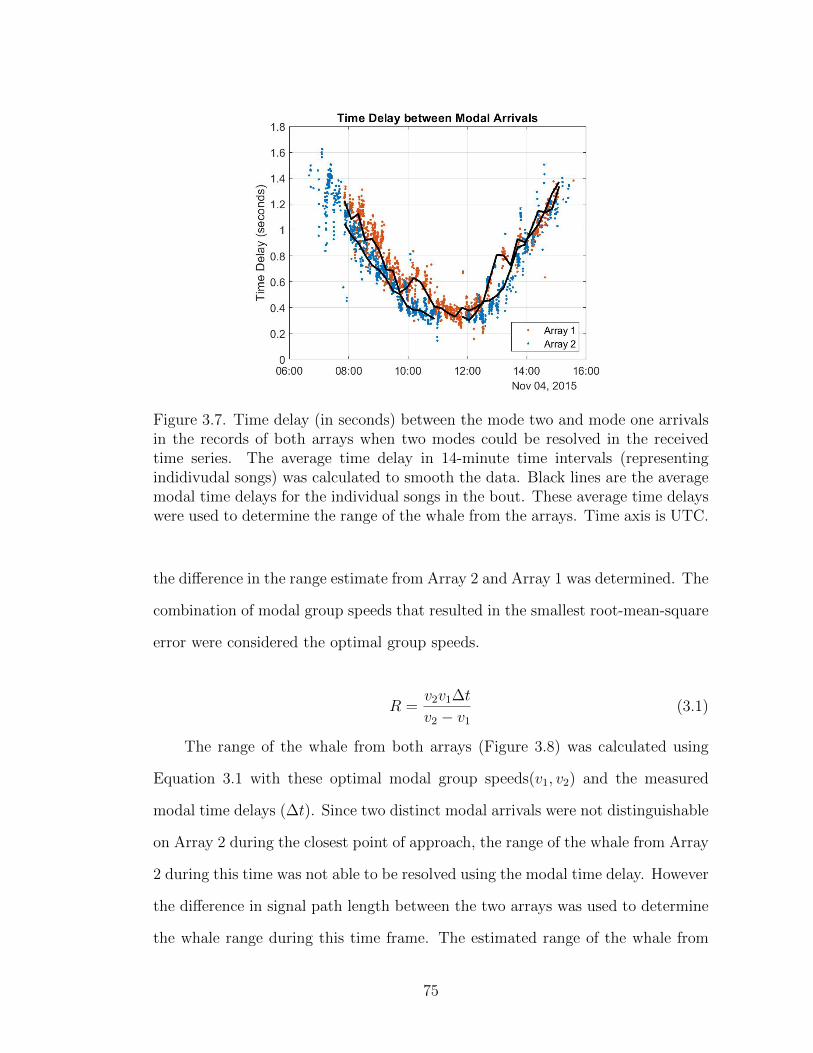
Figure 3.7. Time delay (in seconds) between the mode two and mode one arrivalsin the records of both arrays when two modes could be resolved in the receivedtime series. The average time delay in 14-minute time intervals (representingindidivudal songs) was calculated to smooth the data. Black lines are the averagemodal time delays for the individual songs in the bout. These average time delayswere used to determine the range of the whale from the arrays. Time axis is UTC.
the difference in the range estimate from Array 2 and Array 1 was determined. The
combination of modal group speeds that resulted in the smallest root-mean-square
error were considered the optimal group speeds.
R =v2v1∆t
v2 − v1(3.1)
The range of the whale from both arrays (Figure 3.8) was calculated using
Equation 3.1 with these optimal modal group speeds(v1, v2) and the measured
modal time delays (∆t). Since two distinct modal arrivals were not distinguishable
on Array 2 during the closest point of approach, the range of the whale from Array
2 during this time was not able to be resolved using the modal time delay. However
the difference in signal path length between the two arrays was used to determine
the whale range during this time frame. The estimated range of the whale from
75

Array 1 was adjusted by the range difference to yield an estimate of the whale
range from Array 2 (Figure 3.8 (black line)). The range estimated using both
methods was similar during the whale approach and departure, but the estimate
using the range difference was able to resolve the closest point of approach of the
whale from Array 2.
Figure 3.8. Estimated range of the whale from each array that was calculatedassuming a group speed of 1563 m/s for mode one and a group speed of 1659m/s for mode 2 (blue and orange lines). The whale’s range from Array 2 when itwas closest could not be resolved using the time difference between modes, so therange was estimated using the difference in range (black line). The two methodsof calculating the whale range from Array 2 compare well during the approach anddeparture of the whale. Time axis is UTC.
3.8.2 Localization
The estimate of the whale’s range from the pair of sensors (one from each
array) was used to determine the whale’s track. At each time step, a circle centered
on each sensor with a radius equal to the range of the whale from that sensor was
drawn. The intersection of the two range circles was a potential location of the
whale. There were two intersection points for each time step, which yielded two
76

potential whale tracks. Since the fin pulses were detected on the DMON buoy
before the arrays, the whale was assumed to be traveling from the northeast, so
tracks that showed the whale traveling from the southwest were disregarded. Also a
large number of fin whale calls were not detected on the DNOM after 12:00 (Figure
3.5) and it is unlikely that this whale turned around to travel back towards the
DNOM location at any point during the track. This is supported by observations of
fin whale singers that have been tracked swimming with fairfly consistent directions
of travel (Clark et al., 2019). Therefore, the localization that produced a track with
the fin whale traveling from northeast to southwest was determined to be the most
plausible track (Figure 3.9).
Figure 3.9. Most plausible path that the fin whale traveled on November 4, 2015between 07:00 and 15:30 past the locations of the deployed arrays. Arrow indicatesthe direction of travel from northeast to southwest.
3.9 Inversion for Environmental Properties
The number of modes excited in a waveguide and the group speed of these
modes are sensitive to environmental parameters such as the water depth, sediment
77

layer depth, and the sound speed through water and the sediment. The environ-
mental properties of the study area are not known with a high degree of certainty,
but can be inverted for using the modal group speed estimates used to determine
the whale’s range. The observations of two modal arrivals in the recorded data and
a faster propagating mode two are important since the environmental parameters
must support this type of propagation.
In this study the mode functions for the shallow water environment where
the arrays were deployed were calculated by using the KRAKEN normal mode
program (Porter, 1991). The estimated track shows the fin whale traveling in
water depths of approximately 50 meters, thus a water depth of 50 m with an
isovelocity sound speed profile of 1500 m/s were assumed. Fin whales typically
vocalize while swimming at depths between 10-20 m (Kuna and Nabelek, 2021)
therefore the source was input at a depth of 15 m representing a fin whale vocalizing
at 20-Hz. A layered environment was assumed with 50 m of water overlaying a
sediment layer of unknown depth that extends down to bedrock. The bedrock was
modeled with a compressional sound speed of 3000 m/s and a density of 2.4 g/cc
(Jensen et al., 2011).
KRAKEN was run assuming different combinations of sediment layer depth
and sediment compressional sound speed. The difference between the modeled
modal group speeds and the estimated modal group speeds (v1 = 1593 m/s, v2
= 1659 m/s) was determined and the combination of sediment sound speed and
depth to bedrock input into the model that resulted in the smallest group speed
differences were the most likely environmental parameters. The inversion scheme
predicted a depth to bedrock of 205 meters and a sediment sound speed of 1735
m/s.
78
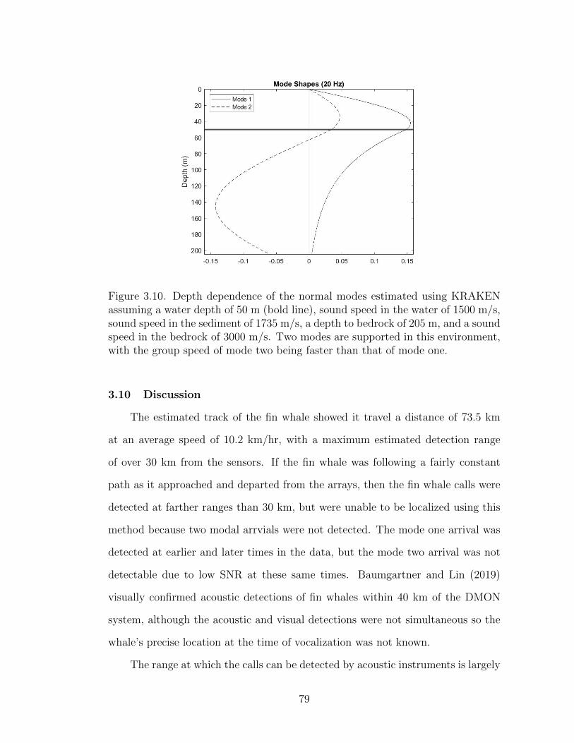
Figure 3.10. Depth dependence of the normal modes estimated using KRAKENassuming a water depth of 50 m (bold line), sound speed in the water of 1500 m/s,sound speed in the sediment of 1735 m/s, a depth to bedrock of 205 m, and a soundspeed in the bedrock of 3000 m/s. Two modes are supported in this environment,with the group speed of mode two being faster than that of mode one.
3.10 Discussion
The estimated track of the fin whale showed it travel a distance of 73.5 km
at an average speed of 10.2 km/hr, with a maximum estimated detection range
of over 30 km from the sensors. If the fin whale was following a fairly constant
path as it approached and departed from the arrays, then the fin whale calls were
detected at farther ranges than 30 km, but were unable to be localized using this
method because two modal arrvials were not detected. The mode one arrival was
detected at earlier and later times in the data, but the mode two arrival was not
detectable due to low SNR at these same times. Baumgartner and Lin (2019)
visually confirmed acoustic detections of fin whales within 40 km of the DMON
system, although the acoustic and visual detections were not simultaneous so the
whale’s precise location at the time of vocalization was not known.
The range at which the calls can be detected by acoustic instruments is largely
79

influenced by environmental conditions. Fin whale 20-Hz pulses have been acousti-
cally detected in shallow water environments at ranges of 30 km (Cholewiak et al.,
2018) and in deep water environments at ranges of 56 km (Sirovic et al., 2007).
The detection range is also sensitive to the local ambient noise levels. Modeled
detection ranges varied between less than 10 km assuming higher ambient noise
conditions out to 100 km at lower ambient noise levels (Stafford et al., 2007).
Previous studies of the bottom sediment types performed in the area of Block
Island, Rhode Island have identified surficial sediment as sand and gravel. Grab
samples and underwater video taken near the Block Island Wind Farm turbine
locations confirmed a seabed dominated by medium and coarse sand, gravel and
cobble sediments (HDR, 2018). Borings taken near the same site characterized
the upper 70 meters of the seafloor and showed a surficial layer of sand and gravel
that overlays layers of sand, clay, and silt (Sheldon, 2012). The estimated sedi-
ment sound speed of 1735 m/s is representative of a sandy environment that has
been observed in this area as described in the studies mentioned. Additionally,
a modeling study performed by Lin et al. (2019) used a sediment sound speed of
1725 m/s for this same study area, which is consistent with the speed of 1735 m/s
estimated in this study. The estimate of 1725 m/s was extracted from the Deck41
seafloor surficial sediment database (Bershad and Weiss, 1976).
Verifying the depth to bedrock is more difficult as few measurements exist.
The available data discuss a depth to bedrock consistent with the estimated depth
of 205 meters. Seismic surveys in this area showed potential bedrock at a depth of
up to and greater than 180 meters below the sea surface (Sheldon, 2012; Needell
et al., 1983).
The current inversion scheme assumes that the water depth, sound speed in
the water, and sediment layer depth is constant over the track of the fin whale.
80
It also assumes that there is a layer of water overlying a single sediment layer
above a basement layer. In reality, the water depth, sound speed, and sediment
layer depth might actually be varying over the fin whale track and there could
be multiple sediment layers with different sound speeds. This variation is not
currently captured in the inversion scheme because it is unknown. Assumptions
can be made to include more detail in the inversion scheme, but the current scheme
produces an average of the environmental parameters over the fin whale track. To
add more detail, the inversion could be run assuming different water depths since
the estimated fin whale track has the whale traveling through various depths. The
inversion scheme could be broken up into different segments based on the water
depth to invert for the varying environmental parameters in these different depth
bins if necessary, but the average values along the track might be enough for specific
applications.
3.11 Conclusion
A fin whale was recorded vocalizing for over eighteen hours on two vertical
line arrays that were deployed off the coast of Block Island, Rhode Island, USA.
The signal received on the arrays arrived as two distinct modes, with mode two
arriving before mode one due to the higher group velocity of the second mode. The
20-Hz pulses observed in this dataset were a single call that arrived as two arrivals
due to modal dispersion and support the hypothesis that the fin whale doublet
calls could be mulitpath arrivals and not produced as a doublet by the whale.
The time delay between the modal arrivals on a single hydrophone and the time
difference in arrival between the mode one arrival on a pair of hydrophones were
used to determine the most likely range and track of the whale from the sensors.
Fin whale detections recorded during the same time period on a separate deployed
system were used to validate the estimated whale track. The modal group speeds
81

and range estimate of the whale were used to invert for the environmental param-
eters of the study area, which resulted in an estimate of the depth to bedrock and
sediment compressional sound speed that were consistent with previous measure-
ments. This paper presents a method of using modal arrivals of fin whale 20-Hz
pulses to estimate a whale’s range using a single sensor and the whale’s location
using a pair of sensors. The analysis could be extended further to invert for the av-
erage environmental parameters along the whale’s track that support the observed
acoustic propagation.
Acknowledgments: The data used for this research was collected as part
of the U.S. Department of the Interior, Bureau of Ocean Energy Management
(BOEM), Environmental Studies Program, Washington, DC under Contract Num-
ber M15PC00002, Task Order M16PD00025. Collaborators in this project include
Randy Gallien and Anwar Khan (HDR, Inc.).
82
Bibliography
Baumgartner, M. F. and Lin, Y.-T. (2019). Evaluating the Accuracy and Detection
Range of a Moored Whale Detection Buoy near the Massachusetts Wind Energy
Area. Technical report, Woods Hole (MA): Massachusetts Clean Energy Center
and U.S. Department of the Interior, Bureau of Ocean Energy Management.OCS
Study BOEM 2019-061.
Bershad, S. and Weiss, M. (1976). Deck41 Surficial Seafloor Sediment De-
scription Database. NOAA National Centers for Environmental Information.
https://doi.org/10.7289/V5VD6WCZ.
Castellote, M., Clark, C. W., and Lammers, M. O. (2012). Fin whale ( Bal-
aenoptera physalus ) population identity in the western Mediterranean Sea.
Marine Mammal Science, 38:325–344.
Cholewiak, D., Clark, C. W., Ponirakis, D., Frankel, A. S., Hatch, L. T., Risch,
D., Stanistreet, J. E., Thompson, M., Vu, E., and Van Parijs, S. M. (2018).
Communicating amidst the noise: modeling the aggregate influence of ambient
and vessel noise on baleen whale communication space in a national marine
sanctuary. Endangered Species Research, 36:59–75.
Clark, C. W., Gagnon, G. J., and Frankel, A. S. (2019). Fin whale singing decreases
with increased swimming speed. Royal Society Open Science, 6.
Croll, D. A., Clark, C. W., Acevedo, A., Tershy, B., Flores, S., Gedamke, J., and
Urban, J. (2002). Only male fin whales sing loud songs. Nature, 417:809.
Cummings, W. C., Thompson, P. O., and Ha, S. J. (1986). Sounds from Bryde,
83

Balaenoptera edeni, and finback, B. physalus, whales in the Gulf of California.
Fishery Bulletin, 84(2):359–370.
Rebull, O. G., Cusı, J. D., Ruiz Fernandez, M., and Muset, J. G. (2006). Tracking
fin whale calls offshore the Galicia Margin, North East Atlantic Ocean. The
Journal of the Acoustical Society of America, 120(4):2077–2085.
HDR (2018). Benthic Monitoring During Wind Turbine Installation and Operation
at the Block Island Wind Farm , Rhode Island. Technical report, Final Report
to the U.S. Department of the Interior, Bureau of Ocean Energy Management,
Office of Renewable Energy Programs.
Helble, T. A., Guazzo, R. A., Alongi, G. C., Martin, C. R., Martin, S. W., and
Henderson, E. E. (2020). Fin Whale Song Patterns Shift Over Time in the
Central North Pacific. Frontiers in Marine Science, 7.
Jensen, F. B., Kuperman, W. A., Porter, M. B., and Schmidt, H. (2011). Compu-
tational Ocean Acoustics. Springer Science, New York, NY, second edition.
Kuna, V. M. and Nabelek, J. L. (2021). Seismic crustal imaging using fin whale
songs. Science, 371:731–735.
Lin, Y.-T., Newhall, A. E., and Lynch, J. F. (2012). Low-frequency broadband
sound source localization using an adaptive normal mode back-propagation ap-
proach in a shallow-water ocean. The Journal of the Acoustical Society of Amer-
ica, 131(2):1798–1813.
Lin, Y.-T., Newhall, A. E., Miller, J. H., Potty, G. R., and Vigness-Raposa, K. J.
(2019). A three-dimensional underwater sound propagation model for offshore
wind farm noise prediction. The Journal of the Acoustical Society of America,
145(5):EL335–EL340.
84
Miksis-Olds, J. L., Harris, D. V., and Heaney, K. D. (2019). Comparison of esti-
mated 20-Hz pulse fin whale source levels from the tropical Pacific and Eastern
North Atlantic Oceans to other recorded populations. Journal of the Acoustical
Society of America, 146(4):2373–2384.
Morano, J. L., Salisbury, D. P., Rice, A. N., Conklin, K. L., Falk, K. L., and
Clark, C. W. (2012). Seasonal and geographical patterns of fin whale song in
the western North Atlantic Ocean. The Journal of the Acoustical Society of
America, 132(2):1207–1212.
Needell, S. W., O’Hara, C. J., and Knebel, H. J. (1983). Maps showing geology
and shallow structure of western Rhode Island Sound: U.S. Geological Survey
Miscellaneous Field Studies Map MF-1537. Technical report, U.S. Geological
Survey.
Nieukirk, S. L., Mellinger, D. K., Moore, S. E., Klinck, K., Dziak, R. P., and
Goslin, J. (2012). Sounds from airguns and fin whales recorded in the mid-
Atlantic Ocean , 1999-2009. The Journal of the Acoustical Society of America,
131(2):1102–1112.
Porter, M. B. (1991). The KRAKEN Normal Mode Program. Technical report,
SACLANT Underwater Research Centre, La Spezia, Italy.
Premus, V. and Spiesberger, J. L. (1997). Can acoustic multipath explain finback
( B. physalus ) 20-Hz doublets in shallow water? The Journal of the Acoustical
Society of America, 101:1127–1138.
Sheldon, D. P. H. (2012). Stratigraphy of a Proposed Wind Farm Site Southeast of
Block Island: Utilization of Borehole Samples, Downhole Logging, and Seismic
Profiles. PhD thesis, University of Rhode Island.
85

Sirovic, A., Hildebrand, J. A., and Wiggins, S. M. (2007). Blue and fin whale call
source levels and propagation range in the Southern Ocean Blue and fin whale
call source levels and propagation range in the Southern Ocean. The Journal of
the Acoustical Society of America, 122(2):1208–1215.
Soule, D. C. and Wilcock, W. S. D. (2013). Fin whale tracks recorded by a seismic
network on the Juan de Fuca Ridge, Northeast Pacific Ocean. The Journal of
the Acoustical Society of America, 133(3):1751–1761.
Stafford, K. M., Mellinger, D. K., Moore, S. E., and Fox, C. G. (2007). Sea-
sonal variability and detection range modeling of baleen whale calls in the Gulf
of Alaska, 1999a¿“2002. The Journal of the Acoustical Society of America,
122(6):3378–3390.
Thompson, P. O., Findley, L. T., and Vidal, O. (1992). 20-Hz pulses and other
vocalizations of fin whales, Balaenopteraphysalus, in the Gulf of California, Mex-
ico. The Journal of the Acoustical Society of America, 92(6):3051–3057.
Urick, R. J. (1983). Principles of Underwater Sound. Peninsula Publishing, Los
Altos, CA, 3rd edition.
Watkins, W. A. (1981). Activities and Underwater Sounds of Fin Whales. Sci.
Rep. Whales Res. Inst, 33:83–117.
Watkins, W. A., Tyack, P., Moore, K. E., and Bird, J. E. (1987). The 20-Hz
signals of finback whales ( Balaenoptera physalus ). The Journal of the Acoustical
Society of America, 82(6):1901–1912.
Weirathmueller, M. J., Stafford, K. M., Wilcock, W. S. D., Hilmo, R. S., Dziak,
R. P., and Trehu, A. M. (2017). Spatial and temporal trends in fin whale
86

vocalizations recorded in the NE Pacific Ocean between 2003-2013. PLOS One,
12(10).
Wiggins, S. M., McDonald, M. A., Munger, L. M., Moore, S. E., and Hildebrand,
J. A. (2004). Wavegu ide Propagation allows for Range Estimates for North
Pacific Right Whales in the Bering Sea. Canadian Acoustics, 32(2):146–154.
87

MANUSCRIPT 4
Analysis and localization of fin whale 20-Hz pulses
This manuscript is currently unpublished.
Jennifer L. Amaral, James H. Miller and Gopu R. Potty
Department of Ocean Engineering, University of Rhode Island, Narragansett, RI
02882, USA
Ying-Tsong Lin
Applied Ocean Physics and Engineering, Woods Hole Oceanographic Institution,
Woods Hole, MA 02543, USA
Kathleen Vigness-Raposa
INSPIRE Environmental, 513 Broadway, Suite 314, Newport, RI 02840, USA
88

Abstract: The 20-Hz pulse, a common fin whale vocalization, was recorded
near continuously for an extended duration off the coast of Block Island, Rhode
Island USA. This fin whale bout was recorded for over eighteen hours as a source of
opporunity during the deployment of multiple sensors in a shallow water environ-
ment. Characteristics of the recorded vocalizations, including the received level,
interpulse interval, and duration of the songs and rest periods were analyzed. The
properties of the recorded song were consistent with those previously reported in
literature. The analysis of the vocalizations revealed that the 20-Hz pulses arrived
at the receivers as multiple modes, where the time delay between modal arrivals
varied with the range of the whale from the receiver. The time delay between
arrivals on spatially separated sensors and the time delay between the modal ar-
rivals on a single sensor were used to localize and track the whale for a duration of
7.2 hours as it swam approximately 73 km past the deployed instruments. [Work
supported by the BOEM]
89
4.1 Introduction
Fin whales (Balaenoptera physalus) produce stereotyped low frequency song
bouts that have been recorded worldwide (Sirovic et al., 2007; Rebull et al., 2006;
Weirathmueller et al., 2017; Thompson et al., 1992; Castellote et al., 2012; Miksis-
Olds et al., 2019). These bouts consist of vocalizations known as 20-Hz pulses that
are repeated at regular intervals to form songs that last for many hours (Watkins
et al., 1987) and are thought to be breeding displays made by male fin whales
(Croll et al., 2002). The 20-Hz pulse is a high-amplitude and short-duration chirp
lasting less than 1 second that sweeps down in frequency between approximately
23 to 18 Hz (Watkins et al., 1987).
Within a song, consecutive 20-Hz pulses occur at consistent time intervals.
This interval is referred to as the interpulse interval and is the time between suc-
cessive pulses measured from a point on one pulse to the same point on a succeeding
pulse (Thompson et al., 1992). The time interval has been known to vary seasonally
(Morano et al., 2012) and can be used to explain a majority of the song variability
between populations in the North Atlantic and North Pacific Oceans (Hatch and
Clark 2004). The fundamental frequencies and intervals between the 20-Hz pulses
are stable with distance and are thought to be the most important signal compo-
nents to the whales (Watkins, 1981). A constant interpulse interval represents a
single pulse pattern while a doublet pattern is represented by a pair of alternating
short and long interpulse intervals (Watkins et al., 1987). The pattern can shift
between doublet and single within a single recorded bout (Thompson et al., 1992).
The stereotyped characteristics and repetition of the 20-Hz pulses for long
duration make the fin whale call well suited for detection, localization, and track-
ing. As fin whales are producing these long duration 20-Hz songs they have been
observed in shallow dive routines (Watkins, 1981) with fairly consistent directions
90
of travel (Clark et al., 2019). The precise range at which fin whales may detect
these signals from a vocalizing whale is not known (Nieukirk et al., 2012), but the
low frequency vocalizations will travel over long distances. The range at which
the calls can be detected by acoustic instruments is largely influenced by envi-
ronmental conditions. Fin whale 20-Hz pulses have been acoustically detected in
shallow water environments at ranges of 30 km (Cholewiak et al., 2018) and in
deep water environments at ranges of 56 km (Sirovic et al., 2007). Baumgartner
and Lin (2019) visually confirmed acoustic detections within 40 km of a deployed
instrument, although the acoustic and visual detections were not simultaneous so
the whale’s precise location at the time of vocalization was not known. The de-
tection range is also sensitive to the local ambient noise levels. Modeled detection
ranges of instruments varied between less than 10 km assuming higher ambient
noise conditions out to 100 km at lower ambient noise levels (Stafford et al., 2007).
For whales vocalizing within the detection range of acoustic instruments, the
20-Hz doublet pattern could be explained by multipath arrivals of a single 20-Hz
pulse at the acoustic instrument rather than the fin whale emitting two pulses at
alternating interpulse intervals (Premus and Spiesberger, 1997). Low frequency
sounds traveling in shallow water experience dispersion of the acoustic normal
modes. A normal mode is described as a standing wave between the boundaries
of an acoustic waveguide that propagates horizontally with a frequency dependent
speed (Jensen et al., 2011). A useful interpretation of an acoustic normal mode is
the interference pattern of upward and downward propagating rays (Mikhalevsky,
2001). Higher mode numbers traditionally correspond to higher grazing angles. A
higher mode (and its corresponding rays) therefore would penetrate deeper into
seafloor at the frequencies of interest to this paper. In shallow water waveguides,
calls received from whales at ranges of more than several water depths may become
91

distorted due to multimode dispersion (Wiggins et al., 2004). A pulse received
on a hydrophone can therefore contain several modal arrivals that traveled at
independent group velocities and arrived at different times. The time difference
between the modal arrivals can be used to calculate the distance between source
and receiver (Lin et al., 2012; Wiggins et al., 2004). Depending on the sound speed
profile in the waveguide and the source frequency, the group velocity of mode 2
could be higher than mode 1 and arrive earlier (Frisk, 1994).
A single bout of 20-Hz fin whale pulses was recorded for an extended duration
on various sensors deployed off the coast of Rhode Island, USA in shallow waters.
The bout was recorded for a duration of eighteen hours, however it is likely that
it lasted longer but was not recorded because the whale was beyond the detection
range of the sensors. The sensors utilized in this study were not deployed for
the purpose of marine mammal localization so the number and position of the
sensors do not allow for typical localization methods to be used. Instead, the
modal arrivals detected in the data on individual sensors were used to localize and
track the whale as it moved past the deployed arrays. A single sensor from each
array was used in the localization process. The characterisitcs of the recorded fin
whale vocalizations as well as the estimated track of the whale will be presented
in this paper.
The paper is organized in the following manner. Section II describes the
study location along with the measurement equipment. Section III presents the
method used to detect the fin whale calls in the dataset. Section IV discusses
the analysis results including properties of the bout, received levels, and the range
difference of the whale in relation to the deployed sensors. Section V presents the
fin whale detections recorded on a different deployed sensor suite that was used to
validate the detections on the deployed arrays. Section VI includes a discussion of
92
modal dispersion, how the recorded data were used to range and track the whale’s
location, and presents the results of the localization. Section VII discusses the
main conclusions of this study.
4.2 Measurement Equipment
Two vertical line arrays (referred to as Array 1 and Array 2) were deployed
for 24 days between October and November 2015 off the coast of Block Island,
Rhode Island, USA (Figure 4.1). These sensor systems were deployed as part of
the Bureau of Ocean Energy Management (BOEM) funded Real-time Opportunity
for Development Environmental Observations (RODEO) program with the objec-
tive of recording the underwater sound generated during impact pile driving to
install the Block Island Wind Farm (BIWF) turbine foundations. Fin whale 20-Hz
vocalizations were recorded as sources of opportunity during the deployment of
the arrays.
Each vertical line array consisted of four HTI-94-SSQ model hydrophones from
High Tech, Inc. with a sensitivity of -170 dB re 1V/µPa, where each hydrophone
was spaced 5 m apart and located at water depths from 20 to 35 m. All sensors
were continuously recording on Several Hydrophone Receive Units (SHRUs) at a
rate of approximately 10 kHz for the duration of deployment. The arrays were
deployed in approximately 40 m of water with an inter-array spacing of 7.5 km.
4.3 Detection Method
A long duration bout of 20-Hz pulses was detected on all of the hydrophones
in the two vertical arrays. Custom scripts were developed in MATLAB R2019a
(www.mathworks.com) to detect and analyze the recorded 20-Hz pulses for the
entire duration of the recording. The acoustic recordings were decimated to a
sampling rate of approximately 1 kHz to allow for more efficient processing and
93
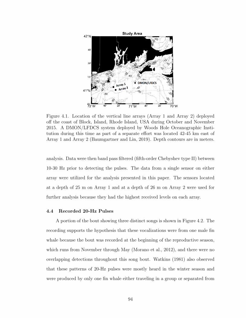
Figure 4.1. Location of the vertical line arrays (Array 1 and Array 2) deployedoff the coast of Block, Island, Rhode Island, USA during October and November2015. A DMON/LFDCS system deployed by Woods Hole Oceanographic Insti-tution during this time as part of a separate effort was located 42-45 km east ofArray 1 and Array 2 (Baumgartner and Lin, 2019). Depth contours are in meters.
analysis. Data were then band pass filtered (fifth-order Chebyshev type II) between
10-30 Hz prior to detecting the pulses. The data from a single sensor on either
array were utilized for the analysis presented in this paper. The sensors located
at a depth of 25 m on Array 1 and at a depth of 26 m on Array 2 were used for
further analysis because they had the highest received levels on each array.
4.4 Recorded 20-Hz Pulses
A portion of the bout showing three distinct songs is shown in Figure 4.2. The
recording supports the hypothesis that these vocalizations were from one male fin
whale because the bout was recorded at the beginning of the reproductive season,
which runs from November through May (Morano et al., 2012), and there were no
overlapping detections throughout this song bout. Watkins (1981) also observed
that these patterns of 20-Hz pulses were mostly heard in the winter season and
were produced by only one fin whale either traveling in a group or separated from
94
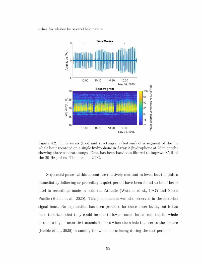
other fin whales by several kilometers.
Figure 4.2. Time series (top) and spectrogram (bottom) of a segment of the finwhale bout recorded on a single hydrophone in Array 2 (hydrophone at 26 m depth)showing three separate songs. Data has been bandpass filtered to improve SNR ofthe 20-Hz pulses. Time axis is UTC.
Sequential pulses within a bout are relatively constant in level, but the pulses
immediately following or preceding a quiet period have been found to be of lower
level in recordings made in both the Atlantic (Watkins et al., 1987) and North
Pacific (Helble et al., 2020). This phenomenon was also observed in the recorded
signal bout. No explanation has been provided for these lower levels, but it has
been theorized that they could be due to lower source levels from the fin whale
or due to higher acoustic transmission loss when the whale is closer to the surface
(Helble et al., 2020), assuming the whale is surfacing during the rest periods.
95
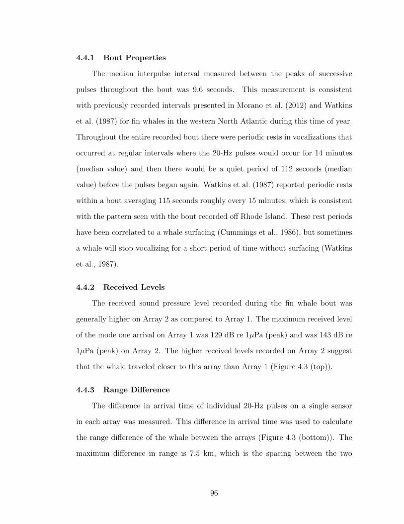
4.4.1 Bout Properties
The median interpulse interval measured between the peaks of successive
pulses throughout the bout was 9.6 seconds. This measurement is consistent
with previously recorded intervals presented in Morano et al. (2012) and Watkins
et al. (1987) for fin whales in the western North Atlantic during this time of year.
Throughout the entire recorded bout there were periodic rests in vocalizations that
occurred at regular intervals where the 20-Hz pulses would occur for 14 minutes
(median value) and then there would be a quiet period of 112 seconds (median
value) before the pulses began again. Watkins et al. (1987) reported periodic rests
within a bout averaging 115 seconds roughly every 15 minutes, which is consistent
with the pattern seen with the bout recorded off Rhode Island. These rest periods
have been correlated to a whale surfacing (Cummings et al., 1986), but sometimes
a whale will stop vocalizing for a short period of time without surfacing (Watkins
et al., 1987).
4.4.2 Received Levels
The received sound pressure level recorded during the fin whale bout was
generally higher on Array 2 as compared to Array 1. The maximum received level
of the mode one arrival on Array 1 was 129 dB re 1µPa (peak) and was 143 dB re
1µPa (peak) on Array 2. The higher received levels recorded on Array 2 suggest
that the whale traveled closer to this array than Array 1 (Figure 4.3 (top)).
4.4.3 Range Difference
The difference in arrival time of individual 20-Hz pulses on a single sensor
in each array was measured. This difference in arrival time was used to calculate
the range difference of the whale between the arrays (Figure 4.3 (bottom)). The
maximum difference in range is 7.5 km, which is the spacing between the two
96

Figure 4.3. Comparison of the peak sound pressure levels (dB re 1µPa) of the 20-Hz pulse measured on both arrays throughout the recorded bout (top). Differencein the path length of the fin whale signals received on a single sensor in botharrays. A positive distance means the signal was received on Array 2 before Array1 and a negative distance means the signal was received on Array 1 before Array2 (bottom). The hydrophone used to generate these data is at a depth of 25 m onArray 1 and 26 m on Array 2. Time axis is UTC.
arrays. This maximum difference in range would be expected when the whale’s
position was directly in line with the two arrays, which would imply the signal
arrived on Array 2 first and then traveled 7.5 km before reaching Array 1.
The received levels recorded on Array 2 were higher than those recorded on
Array 1 up through approximately 13:00, before the received levels became similar
on both arrays (Figure 4.3 (top)). This suggests that the whale was closer to Array
2 up until this time and then the whale traversed a track that was a similar distance
from both arrays. This is confirmed by the variation in the range difference. As
97

the whale approaches the arrays, it is farther from Array 1 than it is from Array
2. The range difference between arrivals is maximum at 11:30, which coincides
with the time of the maximum received sound levels measured on Array 2. This is
the time of the closest point of approach of the whale to the arrays. As the whale
moves away from the arrays, it follows a path bringing it closer to Array 1. After
16:00 it is traveling a path that is closer to Array 1 than Array 2.
4.5 Verification of Detections
A moored buoy system designed to detect, classify, and report the sounds of
large whales in near real time that was part of a separate study (Baumgartner and
Lin, 2019) was deployed near Martha’s Vineyard, Massachusetts, USA during the
same time that the arrays in this study were deployed. The buoy was 45 km east
of Array 1 and 42 km east of Array 2 (Figure 4.1) in a water depth of 34 m and was
equipped with a digital acoustic monitoring (DMON) instrument that was running
a low frequency detection and classification system (LFDCS). The DMON/LFDCS
detects and classifies tonal sounds of baleen whales in near real time and sends the
detection data shore-side to be reviewed. The number of species specific detections
in a 15-minute period within the acoustic detection range of the buoy were made
available to the public after they had been verified.
The DMON/LFDCS automatically detects and classifies fin whales based on
the 20-Hz pulse. Fin whales detected by the DMON/LFDCS had the lowest missed
detection rate compared to other species and had a near real-time false detection
rate of nearly 0 percent. The DMON/LFCDS system was not used for localization,
but the fin-whale specific acoustic detection range of the system was estimated
at 30-40 km (Baumgartner and Lin, 2019). This estimate was based on acoustic
detections and visual sightings at 40 km spatial scales and 24-72 hr temporal scales.
It is possible that the detection range is less or more than this spatial scale since
98

the acoustic and visual detections were not simultaneous, although this detection
range was consistent with the 30 km detection range determined by Cholewiak
et al. (2018) in a similar shallow environment of Massachusetts Bay.
The detection record of fin whales on November 4, 2015 showed that the
DMON/LFDCS detected the largest number of fin whale 20-Hz pulses about 6
hours and 45 minutes before the highest sound levels were measured on the arrays
(Figure 4.4). It is assumed that the pulses recorded on the arrays were made by a
single fin whale and that the DMON detections are of that same whale. Examples
of DMON recorded data show a single fin whale 20-Hz pulse that repeats at regular
intervals of approximately every 10 seconds (pitch track (PT) data for 11/03/15
23:19:32 EST available on http://dcs.whoi.edu/nomans0315/nomans0315.shtml),
which is similar to what was recorded on the arrays. From the time series of
DMON/LFDCS detections it was inferred that the fin whale traveled through the
detection range of the system toward the array locations and was beyond the
detection range of the DMON at the time of the highest measured sound levels
on the arrays. Since the arrays were able to detect the fin whale calls during the
earlier times, it is assumed that the detection range of the arrays is farther than
the 40 km DMON detection range.
4.6 Mode Dispersion and Source Localization
The normal mode approach is typically used to describe low frequency sound
propagation in shallow water environments. A mode is described as a standing
wave between the boundaries of an acoustic waveguide that propagates horizontally
with a frequency dependent speed (Jensen et al., 2011). The group velocity of a
mode is the velocity at which energy in the mode is transported. A signal measured
on a receiver will be the summation of all of the modes, however, individual modes
traveling at different group velocities will arrive at different times (Urick, 1983).
99
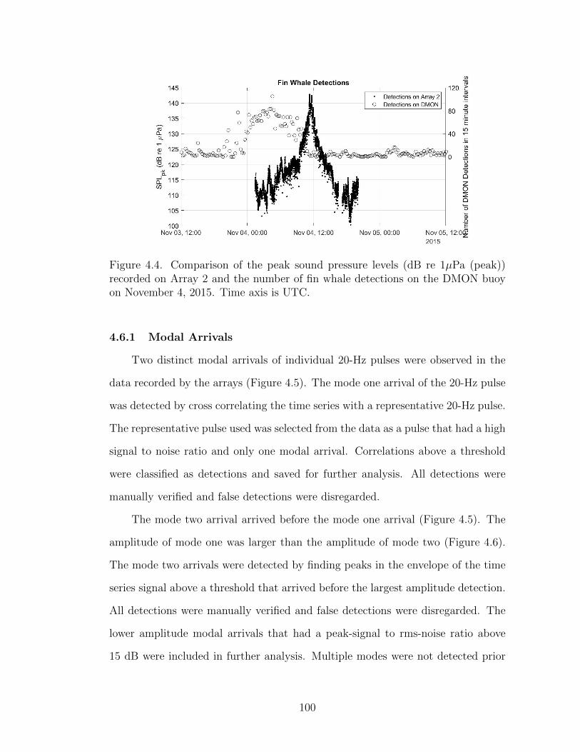
Figure 4.4. Comparison of the peak sound pressure levels (dB re 1µPa (peak))recorded on Array 2 and the number of fin whale detections on the DMON buoyon November 4, 2015. Time axis is UTC.
4.6.1 Modal Arrivals
Two distinct modal arrivals of individual 20-Hz pulses were observed in the
data recorded by the arrays (Figure 4.5). The mode one arrival of the 20-Hz pulse
was detected by cross correlating the time series with a representative 20-Hz pulse.
The representative pulse used was selected from the data as a pulse that had a high
signal to noise ratio and only one modal arrival. Correlations above a threshold
were classified as detections and saved for further analysis. All detections were
manually verified and false detections were disregarded.
The mode two arrival arrived before the mode one arrival (Figure 4.5). The
amplitude of mode one was larger than the amplitude of mode two (Figure 4.6).
The mode two arrivals were detected by finding peaks in the envelope of the time
series signal above a threshold that arrived before the largest amplitude detection.
All detections were manually verified and false detections were disregarded. The
lower amplitude modal arrivals that had a peak-signal to rms-noise ratio above
15 dB were included in further analysis. Multiple modes were not detected prior
100

Figure 4.5. Time series (top) and spectrogram (bottom) showing three fin whale20-Hz pulses recorded on a single hydrophone in Array 1. Two distinct and timeseparated arrivals are clearly seen in both the time series and spectrogram rep-resentation. The interpulse interval between the larger amplitude arrivals (modeone) is approximately 10 seconds. The receiver was at 25 meters depth. Time axisis UTC.
to 07:00 and later than 15:30 in the dataset because the SNR of the higher order
modes was not greater then the ambient noise levels.
4.6.2 Time Delay between Modal Arrivals
The time delay between the mode two and mode one arrivals within an in-
dividual 20-Hz pulse on a single sensor was calculated. The time delay data was
smoothed by taking the average time delay in each song. The median song duration
was 14 minutes long, so the average time delay was taken every 14 minutes.
The time delay between the arrivals in the mode pairs from Figure 4.6 was
101

Figure 4.6. Peak sound pressure levels (dB re 1µPa (peak)) of the individual modalarrivals on a single sensor in each array. The sensor was at a depth of 25 m inArray 1 and 26 m in Array 2. Time axis is UTC.
calculated. The time difference between the modal arrivals on a single hydrophone
varied throughout the recording (Figure 4.7) and was a function of the range of
the whale from the sensor. The time difference between arrivals was greater at
earlier times and decreased as the whale approached the array. Only one arrival
was identifiable in the data from Array 2 when the whale was closest, although
two arrivals were seen in the data from Array 1 during this same time.
4.6.3 Range Estimate
The range of the whale from each array was calculated using Equation 4.1,
where R is the range of the whale in meters, v is the group speed of the indicated
modal arrival, and ∆t is the difference in arrival time between the two modes as
102
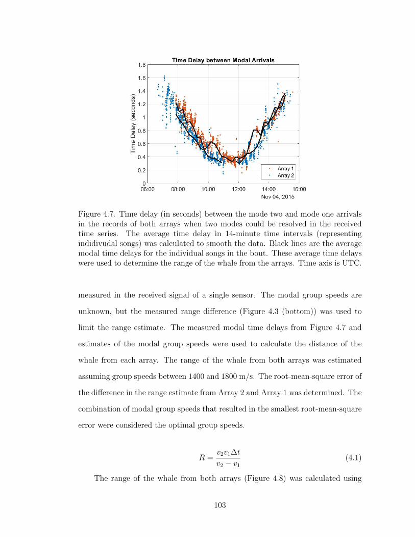
Figure 4.7. Time delay (in seconds) between the mode two and mode one arrivalsin the records of both arrays when two modes could be resolved in the receivedtime series. The average time delay in 14-minute time intervals (representingindidivudal songs) was calculated to smooth the data. Black lines are the averagemodal time delays for the individual songs in the bout. These average time delayswere used to determine the range of the whale from the arrays. Time axis is UTC.
measured in the received signal of a single sensor. The modal group speeds are
unknown, but the measured range difference (Figure 4.3 (bottom)) was used to
limit the range estimate. The measured modal time delays from Figure 4.7 and
estimates of the modal group speeds were used to calculate the distance of the
whale from each array. The range of the whale from both arrays was estimated
assuming group speeds between 1400 and 1800 m/s. The root-mean-square error of
the difference in the range estimate from Array 2 and Array 1 was determined. The
combination of modal group speeds that resulted in the smallest root-mean-square
error were considered the optimal group speeds.
R =v2v1∆t
v2 − v1(4.1)
The range of the whale from both arrays (Figure 4.8) was calculated using
103
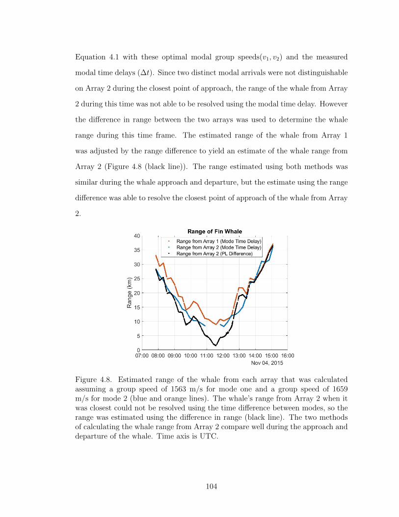
Equation 4.1 with these optimal modal group speeds(v1, v2) and the measured
modal time delays (∆t). Since two distinct modal arrivals were not distinguishable
on Array 2 during the closest point of approach, the range of the whale from Array
2 during this time was not able to be resolved using the modal time delay. However
the difference in range between the two arrays was used to determine the whale
range during this time frame. The estimated range of the whale from Array 1
was adjusted by the range difference to yield an estimate of the whale range from
Array 2 (Figure 4.8 (black line)). The range estimated using both methods was
similar during the whale approach and departure, but the estimate using the range
difference was able to resolve the closest point of approach of the whale from Array
2.
Figure 4.8. Estimated range of the whale from each array that was calculatedassuming a group speed of 1563 m/s for mode one and a group speed of 1659m/s for mode 2 (blue and orange lines). The whale’s range from Array 2 when itwas closest could not be resolved using the time difference between modes, so therange was estimated using the difference in range (black line). The two methodsof calculating the whale range from Array 2 compare well during the approach anddeparture of the whale. Time axis is UTC.
104

4.6.4 Estimate of Whale Track
The estimate of the whale’s range from both arrays was used to determine
the whale’s track. At each time step, a circle centered on each array with a radius
equal to the range of the whale from that array was drawn. The intersection of the
two range circles was a potential location of the whale. There were two intersection
points for each time step, which yielded two potential whale tracks. Since the fin
pulses were detected on the DMON buoy before the arrays, the whale was assumed
to be traveling from the northeast, so tracks that showed the whale traveling from
the southwest were disregarded. Also large number of fin whale calls were not
detected on the DMON after 12:00 (Figure 4.4) and it is unlikely that this whale
turned around to travel back towards the DMON location at any point during
the track. This is supported by observations of fin whale singers that been tracked
swimming with fairly consistent directions of travel (Clark et al., 2019). Therefore,
the localization that produced a track with the fin whale traveling from northeast
to southwest was determined to be the most plausible track (Figure 4.9).
4.6.5 Speed and Track of Whale
The whale was tracked for a total distance of 73.5 km for a duration of 7.2
hours. The average swim speed of the whale along this track was 10.2 km/hr. This
is consistent with fin whale speeds and tracks that have been previously reported
in literature. Clark et al. (2019) tracked fin whales as they sang for 15.8 hours
(mean) and traveled 86.2 km (mean) at speeds of 6.7 km/hr (mean). Fin whales in
the North Pacific were tracked while they swam distances of 18 km (mean) over 6.9
hours (mean) at speeds of 3 km/hr (mean) (Soule and Wilcock, 2013). Kuna and
Nabelek (2021) also tracked whales in the North Pacific as they covered distances
between 16-38 km at speeds between 4.1 and 10.3 km/hr.
105

Figure 4.9. Most plausible path that the fin whale traveled on November 4, 2015between 07:00 and 15:30 past the locations of the deployed arrays. Arrow indicatesthe direction of travel from northeast to southwest.
4.7 Conclusion
A fin whale was recorded vocalizing for over eighteen hours on two vertical line
arrays that were deployed off the coast of Block Island, Rhode Island, USA. The
20-Hz pulses were emitted with a regular interpulse interval as the whale traveled
a northeast to southwest track past the array locations. The signal received on
the vertical line arrays arrived as two distinct modes, with mode two arriving
before mode one due to the higher group velocity of the second mode. The 20-Hz
pulses observed in this dataset were a single call that arrived as two arrivals due
to modal dispersion and support the hypothesis that the fin whale doublet calls
could be mulitpath arrivals and not produced as a doublet by the whale. The time
delay between the modal arrivals on a single hydrophone and the time difference in
arrival between the mode one arrival on two spatially separated hydrophones were
used to determine the most likely range and track of the whale from the sensors.
Fin whale detections on a separate system were used to inform the estimated whale
106

track.
Acknowledgments: The data used for this research was collected as part
of the U.S. Department of the Interior, Bureau of Ocean Energy Management
(BOEM), Environmental Studies Program, Washington, DC under Contract Num-
ber M15PC00002, Task Order M16PD00025. Collaborators in this project include
Randy Gallien and Anwar Khan (HDR, Inc.).
107

Bibliography
Baumgartner, M. F. and Lin, Y.-T. (2019). Evaluating the Accuracy and Detection
Range of a Moored Whale Detection Buoy near the Massachusetts Wind Energy
Area. Technical report, Woods Hole (MA): Massachusetts Clean Energy Center
and U.S. Department of the Interior, Bureau of Ocean Energy Management.OCS
Study BOEM 2019-061.
Castellote, M., Clark, C. W., and Lammers, M. O. (2012). Fin whale ( Bal-
aenoptera physalus ) population identity in the western Mediterranean Sea.
Marine Mammal Science, 38:325–344.
Cholewiak, D., Clark, C. W., Ponirakis, D., Frankel, A. S., Hatch, L. T., Risch,
D., Stanistreet, J. E., Thompson, M., Vu, E., and Van Parijs, S. M. (2018).
Communicating amidst the noise: modeling the aggregate influence of ambient
and vessel noise on baleen whale communication space in a national marine
sanctuary. Endangered Species Research, 36:59–75.
Clark, C. W., Gagnon, G. J., and Frankel, A. S. (2019). Fin whale singing decreases
with increased swimming speed. Royal Society Open Science, 6.
Croll, D. A., Clark, C. W., Acevedo, A., Tershy, B., Flores, S., Gedamke, J., and
Urban, J. (2002). Only male fin whales sing loud songs. Nature, 417:809.
Cummings, W. C., Thompson, P. O., and Ha, S. J. (1986). Sounds from Bryde,
Balaenoptera edeni, and finback, B. physalus, whales in the Gulf of California.
Fishery Bulletin, 84(2):359–370.
Frisk, G. V. (1994). Ocean and Seabed Acoustics. Prentice-Hall, Inc, Englewood
Cliffs, New Jersey.
108
Rebull, O. G., Cusı, J. D., Ruiz Fernandez, M., and Muset, J. G. (2006). Tracking
fin whale calls offshore the Galicia Margin, North East Atlantic Ocean. The
Journal of the Acoustical Society of America, 120(4):2077–2085.
HDR (2018). Benthic Monitoring During Wind Turbine Installation and Operation
at the Block Island Wind Farm , Rhode Island. Technical report, Final Report
to the U.S. Department of the Interior, Bureau of Ocean Energy Management,
Office of Renewable Energy Programs.
Helble, T. A., Guazzo, R. A., Alongi, G. C., Martin, C. R., Martin, S. W., and
Henderson, E. E. (2020). Fin Whale Song Patterns Shift Over Time in the
Central North Pacific. Frontiers in Marine Science, 7.
Jensen, F. B., Kuperman, W. A., Porter, M. B., and Schmidt, H. (2011). Compu-
tational Ocean Acoustics. Springer Science, New York, NY, second edition.
Kuna, V. M. and Nabelek, J. L. (2021). Seismic crustal imaging using fin whale
songs. Science, 371:731–735.
Lin, Y.-T., Newhall, A. E., and Lynch, J. F. (2012). Low-frequency broadband
sound source localization using an adaptive normal mode back-propagation ap-
proach in a shallow-water ocean. The Journal of the Acoustical Society of Amer-
ica, 131(2):1798–1813.
Lin, Y.-T., Newhall, A. E., Miller, J. H., Potty, G. R., and Vigness-Raposa, K. J.
(2019). A three-dimensional underwater sound propagation model for offshore
wind farm noise prediction. The Journal of the Acoustical Society of America,
145(5):EL335–EL340.
Mikhalevsky, P. N (2001). Arctic Acoustics. Encyclopedia of Ocean Sciences, J.H.
Steele, ed., vol. 1, pp 53-61, Elsevier Ltd.
109
Miksis-Olds, J. L., Harris, D. V., and Heaney, K. D. (2019). Comparison of esti-
mated 20-Hz pulse fin whale source levels from the tropical Pacific and Eastern
North Atlantic Oceans to other recorded populations. Journal of the Acoustical
Society of America, 146(4):2373–2384.
Morano, J. L., Salisbury, D. P., Rice, A. N., Conklin, K. L., Falk, K. L., and
Clark, C. W. (2012). Seasonal and geographical patterns of fin whale song in
the western North Atlantic Ocean. The Journal of the Acoustical Society of
America, 132(2):1207–1212.
Needell, S. W., O’Hara, C. J., and Knebel, H. J. (1983). Maps showing geology
and shallow structure of western Rhode Island Sound: U.S. Geological Survey
Miscellaneous Field Studies Map MF-1537. Technical report, U.S. Geological
Survey.
Nieukirk, S. L., Mellinger, D. K., Moore, S. E., Klinck, K., Dziak, R. P., and
Goslin, J. (2012). Sounds from airguns and fin whales recorded in the mid-
Atlantic Ocean , 1999-2009. The Journal of the Acoustical Society of America,
131(2):1102–1112.
Porter, M. B. (1991). The KRAKEN Normal Mode Program. Technical report,
SACLANT Underwater Research Centre, La Spezia, Italy.
Premus, V. and Spiesberger, J. L. (1997). Can acoustic multipath explain finback
( B. physalus ) 20-Hz doublets in shallow water? The Journal of the Acoustical
Society of America, 101:1127–1138.
Sheldon, D. P. H. (2012). Stratigraphy of a Proposed Wind Farm Site Southeast of
Block Island: Utilization of Borehole Samples, Downhole Logging, and Seismic
Profiles. PhD thesis, University of Rhode Island.
110

Sirovic, A., Hildebrand, J. A., and Wiggins, S. M. (2007). Blue and fin whale call
source levels and propagation range in the Southern Ocean Blue and fin whale
call source levels and propagation range in the Southern Ocean. The Journal of
the Acoustical Society of America, 122(2):1208–1215.
Soule, D. C. and Wilcock, W. S. D. (2013). Fin whale tracks recorded by a seismic
network on the Juan de Fuca Ridge, Northeast Pacific Ocean. The Journal of
the Acoustical Society of America, 133(3):1751–1761.
Stafford, K. M., Mellinger, D. K., Moore, S. E., and Fox, C. G. (2007). Sea-
sonal variability and detection range modeling of baleen whale calls in the Gulf
of Alaska, 1999a¿“2002. The Journal of the Acoustical Society of America,
122(6):3378–3390.
Thompson, P. O., Findley, L. T., and Vidal, O. (1992). 20-Hz pulses and other
vocalizations of fin whales, Balaenopteraphysalus, in the Gulf of California, Mex-
ico. The Journal of the Acoustical Society of America, 92(6):3051–3057.
Urick, R. J. (1983). Principles of Underwater Sound. Peninsula Publishing, Los
Altos, CA, 3rd edition.
Watkins, W. A. (1981). Activities and Underwater Sounds of Fin Whales. Sci.
Rep. Whales Res. Inst, 33:83–117.
Watkins, W. A., Tyack, P., Moore, K. E., and Bird, J. E. (1987). The 20-Hz
signals of finback whales ( Balaenoptera physalus ). The Journal of the Acoustical
Society of America, 82(6):1901–1912.
Weirathmueller, M. J., Stafford, K. M., Wilcock, W. S. D., Hilmo, R. S., Dziak,
R. P., and Trehu, A. M. (2017). Spatial and temporal trends in fin whale
111
vocalizations recorded in the NE Pacific Ocean between 2003-2013. PLOS One,
12(10).
Wiggins, S. M., McDonald, M. A., Munger, L. M., Moore, S. E., and Hildebrand,
J. A. (2004). Wavegu ide Propagation allows for Range Estimates for North
Pacific Right Whales in the Bering Sea. Canadian Acoustics, 32(2):146–154.
112


