1
Combined Processing of
GPS, GLONASS, and SBAS
Code Phase and Carrier Phase Measurements
Lambert Wanninger, Stephan Wallstab-Freitag
Geodetic Institute, Dresden University of Technology, Germany
BIOGRAPHY
Lambert Wanninger received his Dipl.-Ing. and his Dr.-
Ing. in Geodesy from the University of Hannover, Ger-
many. He spent several years at Dresden University of
Technology working in the field of GPS. In 2000 he
founded Ingenieurbüro Wanninger, which develops soft-
ware for precise GNSS applications. In 2004 he rejoined
Dresden University of Technology as a professor in the
Geodetic Institute.
Stephan Wallstab-Freitag received his Dipl.-Ing. in Geod-
esy from Dresden University of Technology. He spent one
year at the Geodetic Institute at Dresden University of
Technology working in the field of GNSS. Recently he
joined GOM at Braunschweig, Germany, a company
which develops optical 3D measurement techniques.
ABSTRACT
Precise (centimetre level) applications require code and
carrier phase pseudoranges and differential positioning
including carrier phase ambiguity resolution. Objective of
this research work is to combine GPS with GLONASS
and single-frequency SBAS ranging to gain improved
availability, faster ambiguity resolution, and higher accu-
racy. Although GLONASS and SBAS broadcast orbits
and often code observations are of lower accuracy than
those of GPS, carrier phase observations are of similar
quality. In contrast to GPS, GLONASS requires the esti-
mation of inter-channel biases and SBAS multipath ef-
fects of static observations produce biases in the coordi-
nates. Nevertheless, RTK (Real Time Kinematic) and fast
static positioning improves considerably if all existing
ranging signals are used.
INTRODUCTION
One of the main limitations of GPS is the small number of
satellite signals being available to the user at any one
time. In future many more satellites, e.g. of the European
Galileo and the Chinese Compass system, will broadcast
ranging signals. But even today additional signals are
available. Not only that the satellites of the Russian
GLONASS provide ranging signals, also the SBAS (i.e.
WAAS, EGNOS, MSAS, and GAGAN) satellites enable
the users to produce code and carrier phase observations.
In early 2006 several manufacturers of GPS equipment
added GLONASS capability to their products. Today
many of the dual-frequency receivers on the market are
combined GPS/GLONASS receivers. The additional ob-
servations are used to gain improved availability and
faster ambiguity resolution. The GLONASS-specific dif-
ficulty of inter-channel biases (or differential hardware
delays) got new importance because now, often mixed
baselines are observed. Receiving equipment of the same
type may experience similar inter-channel biases so that
these biases may almost completely be removed in differ-
ential mode (Zinoviev 2005). In mixed baselines, how-
ever, the inter-channel biases have to be estimated as ad-
ditional parameters in the position computation.
Although ranging to the SBAS satellites is one of the
main objectives of these augmentation systems (e.g. Ven-
tura-Traveset et al. 2006), this service has seldom been
used for precise positioning yet. The presently available
single-frequency signals limit the use of SBAS ranging
for precise applications to short baselines, where iono-
spheric effects cancel out by differencing. In future dual-
frequency SBAS signals may be available (Soddu et al.
2005) which will make SBAS ranging even more attrac-
tive for precise applications.
_______________________________________ Proc. ION GNSS 2007, Fort Worth, Tx., Sep. 25-28, 2007,
pp. 866-875.
2
A coarse estimate of the improvement of positioning per-
formance when adding additional satellite signals can be
based on calculated DOP values. Average values for
Dresden, Germany reveal that the additional code or car-
rier phase observations on the signals of the four available
geostationary SBAS satellites have a larger positive effect
than the 11 GLONASS satellites orbiting in medium
heights (Tab. 1). When adding GLONASS and SBAS to
the existing GPS constellation twice as many satellite
signals are available on average and the DOP values de-
crease by approximately 25 % as compared to GPS only.
Tab.1: Expected improvement of positioning performance
due to an increased number of GNSS satellites, average
DOP values calculated for Dresden, Germany, July 2007,
10° elevation mask.
GPS
(30 SV)
GPS+
GLON-
ASS
(30+11)
GPS+
SBAS
(30+4)
GPS+
GLONASS+
SBAS
(30+11+4)
∅ visible SV 8.4 11.7 12.4 15.7
NDOP 0.85 0.72 0.60 0.55 EDOP 0.65 0.60 0.54 0.50 VDOP 1.59 1.36 1.34 1.21
PDOP 1.93 1.66 1.57 1.43
GLONASS ORBITS AND CODE PHASE OBSER-
VATIONS
There are several differences between GPS and GLON-
ASS which need to be taken into account performing
combined processing. Among these are different geodetic
reference systems (WGS-84 versus PZ-90 or PZ-90.02
after September 19, 2007) and offsets between system
times including leap second differences. These differences
are removed by applying appropriate transformation pa-
rameters (see e.g. Zinoviev 2005, ICD 2002).
Other differences between GPS and GLONASS have to
be dealt with through proper weighting of the observables
or by estimating additional parameters. One effect is
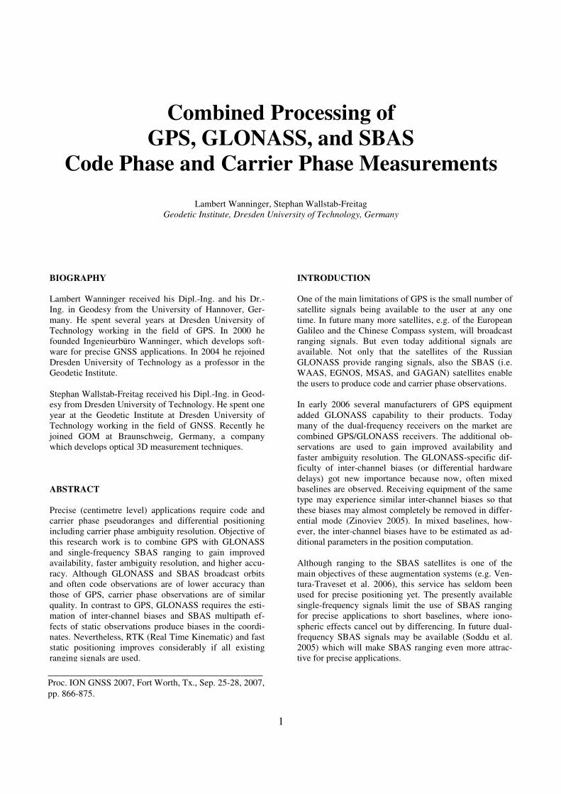
caused by large differences of orbit accuracies. Presently
GLONASS broadcast orbits are worse by a factor of 3 as
compared to GPS (Fig. 1). The effect of this accuracy
difference on differential GNSS depends on the baseline
length and the positioning mode selected. For code-based
single-frequency GNSS or phase-based short baseline
RTK hardly any effect can be seen. However, precise dif-
ferential carrier phase positioning on longer baselines (10
km+) is affected. For all post-processing applications on
longer baselines it is recommended to use precise IGS
orbits. But even here, accuracy differences exist: precise
IGS GLONASS orbits are of lower accuracy (15 cm) than
precise IGS GPS final orbits (<5 cm) (IGS 2007). This
affects just very long baselines (100+ km).
Fig. 1: 3D-accuracy of broadcast ephemeris, based on JPL
Analysis Reports (GPS) and IGS IGLOS Orbit Combina-
tion Reports (GLONASS).
A further difference lies in the code phase observation
quality, which depends on multipath effects and random
noise. The GLONASS chip lengths of C/A- and P-codes
are twice as large as the chip lengths of the GPS codes
(ICD 2002, IS-GPS 2004). Therefore, one would expect a
somewhat lower quality of the GLONASS code phase
observables as compared to GPS.
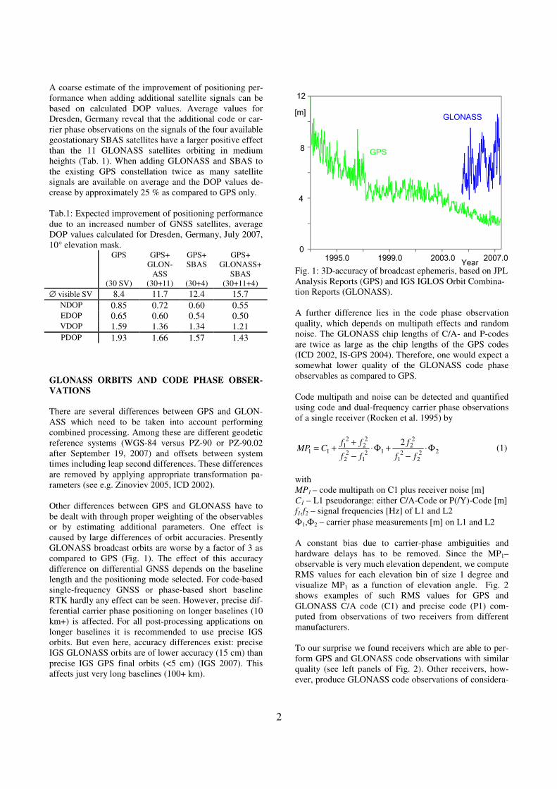
Code multipath and noise can be detected and quantified
using code and dual-frequency carrier phase observations
of a single receiver (Rocken et al. 1995) by
222
21
22
121
22
22
21
11
2Φ⋅
−+Φ⋅
−
++=
ff
f
ff
ffCMP (1)
with
MP1 – code multipath on C1 plus receiver noise [m]
C1 – L1 pseudorange: either C/A-Code or P(/Y)-Code [m]
f1,f2 – signal frequencies [Hz] of L1 and L2
Φ1,Φ2 – carrier phase measurements [m] on L1 and L2
A constant bias due to carrier-phase ambiguities and
hardware delays has to be removed. Since the MP1–
observable is very much elevation dependent, we compute
RMS values for each elevation bin of size 1 degree and
visualize MP1 as a function of elevation angle. Fig. 2
shows examples of such RMS values for GPS and
GLONASS C/A code (C1) and precise code (P1) com-
puted from observations of two receivers from different
manufacturers.
To our surprise we found receivers which are able to per-
form GPS and GLONASS code observations with similar
quality (see left panels of Fig. 2). Other receivers, how-
ever, produce GLONASS code observations of considera-
3
bly lower quality as compared to GPS (right panels of Fig.
2). In case of the standard accuracy signal (C/A code)
GLONASS observations are here always of lower accu-
racy (upper right panel). We take this into account by giv-
ing the GLONASS code observations a lower weight.
The situation is different for the precise code (lower right
panel). Here, the two RMS curves intersect because the
GLONASS code-correlation channels perform better than
the code-free GPS observation technique for signals of
low elevated satellites.
Fig. 2: Comparison of the elevation dependence of MP1
values for two different receiver types and different code
phase observables on L1: C/A-code C1 and precise code
P1.
GLONASS INTER-CHANNEL BIASES
One of the main differences of GLONASS in comparison
to GPS is the Frequency Division Multiple Access
(FDMA) approach, which results in the use of several
adjacent frequencies for the broadcast signals. Further-
more, none of the many GLONASS frequencies is exactly
identical with one of the two GPS frequencies. Conse-
quently, different hardware biases exist in GPS and
GLONASS receiving channels as well as between
GLONASS channels. It is expected that these inter-
channel delays may change in time due to, for example,
temperature changes (Dodson et al. 1999). Receiving
equipment of the same type may experience similar inter-
channel biases so that they can almost completely be re-
moved in differential mode (Zinoviev 2005).
Thus, the combined processing of GPS and GLONASS
carrier phase observations in differential mode requires
the estimation of two independent receiver clock un-
knowns, one for the GPS signals and one for GLONASS.
In addition, the GLONASS inter-channel biases need to
be estimated as well. Pratt et al. (1998) suggested that the
inter-channel biases are linearly dependent on signal fre-
quency. We have estimated inter-channel biases in several
ten baselines of various GPS/GLONASS-receivers and
always found a dominant linear dependence.
This experience with GPS and GLONASS (and SBAS)
carrier phase observations led to the following observa-
tion equations for single-difference observables ∆Φ [m]:
( ))3(
)2(
,
,,0,,
,
,
/,0,
,/,
∆Φ
∆Φ
+∆⋅+
∆⋅+∆⋅+∆=∆Φ
+∆⋅+
∆⋅+∆=∆Φ
ελ
δδ
ελ
δ
iba
Glonassba
iGlonassba
iba
iGlonassba
iba
SBASGPSba
iba
iSBASGPSba
N
hktcR
N
tcR
Subscripts a,b stand for the stations involved, the super-
script GPS, or Glonass (or SBAS) indicates the GNSS
satellite system, the superscript i specifies the individual
satellite number. Furthermore,
R∆ - single difference of ranges satellite – re-
ceiver [m], which is a function of the base-
line coordinates,
0c - speed of light in vacuum [m/s],
Systemtδ∆ - Difference of receiver clocks, which are
different for GPS and GLONASS due to
different hardware delays in the receivers
[s], Glonass
hδ∆ - Difference of inter-channel biases of the
two receivers for adjacent GLONASS fre-
quencies [s],
k - GLONASS channel number [-],
λ - signal wavelength [m],
N∆ - single difference of carrier phase ambiguity
[-],
∆Φε - sum of all uncorrected systematic and ran-
dom errors in the single-difference observ-
able [m].
This approach was realized in the baseline software Wa1
including a combined ambiguity fixing for both, GPS and
GLONASS observations. Wa1 processing is based on
single-difference observations. It thus avoids all the diffi-
culties of GLONASS ambiguity resolution which occur if
double-difference observables are used. All baseline proc-
essing results presented in this paper were produced using
this software.
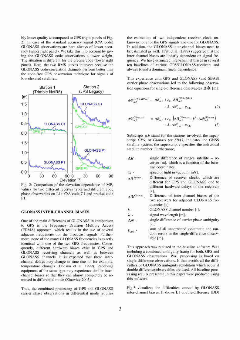
Fig.3 visualizes the difficulties caused by GLONASS
inter-channel biases. It shows L1 double-difference (DD)
4
residuals of two short baselines, one observed with re-
ceivers of the same type, the other observed with receiv-
ers from different manufacturers. Ground truth baseline
coordinates were obtained from several days of GPS ob-
servations. Antenna phase centre corrections were ap-
plied. Carrier phase ambiguities were estimated and fixed,
i.e. removed. What remains in the DD residuals are the
remaining effects of uncorrected systematic and random
errors. In this short baseline they are mainly caused by
multipath. In the case of GLONASS observations inter-
channel biases may have a large effect as well. In the
baseline with two receivers of the same type, these inter-
channel biases are so small, that they have hardly any
effect on the estimated coordinates (Fig. 3). In the mixed
baseline, however, they reach more than 2 cm for adjacent
GLONASS frequencies. This means that the maximum
effect on double differences reaches more than one L1
wavelength for this receiver combination and a presently
maximum channel number difference of 12max =∇k .
An important aspect for the handling of these GLONASS
inter-channel biases is their stability in time and their de-
pendence on temperature. In order to obtain a better un-
derstanding we conducted several experiments. The re-
sults of two of these experiments are presented here.
First of all we were interested in the long term stability of
these inter-channel biases. This requires long-term obser-
vations of two receivers with a small distance between
their antennas. We found an appropriate data set from the
IGS station Wettzell in Germany. At this site several GPS
and GPS/GLONASS receivers are operated simultane-
ously. The observation data is available from the servers
of Bundesamt für Kartographie und Geodäsie (BKG) in
Frankfurt, Germany. From end of 2002 until early 2004
two GPS/GLONASS receivers from different manufac-
turers were operated: an Ashtech Z-18 at station WTZZ
and a JPS Legacy at station WTZJ. The distance between
the two antennas was just 2.5 m.
We processed all daily observation files with Wa1 soft-
ware, fixed the carrier-phase ambiguities and estimated
the inter-channel bias differencesGlonass
hδ∆ , one value
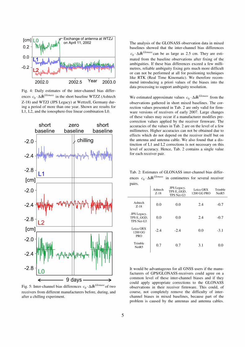
per day (Fig. 4). The peak to peak variations of the esti-
mated values are about 1 mm and thus very small. No
seasonal (temperature) effects and no aging effects are
observed. A jump, however, occurred when the antenna
was exchanged from TRM29659.00 NONE to JPSRE-
GANT_SD_E NONE at station WTZJ on April 4, 2002.
Furthermore, we tried to determine the temperature de-
pendence of the inter-channel biases. We conducted ex-
periments similar to those of Dodson et al. 1999. We re-
corded observations of 2 GPS/GLONASS receivers of a
short baseline or zero baseline. One of the receivers, a
Leica GRX 1200 GG PRO, was chilled for several hours.
The temperature difference at the outside of the receiver
reached more than 20 degrees Celsius. Unfortunately, we
were not able to determine the inside temperature of the
equipment. The other receiver, a JPS Legacy, remained
unchanged.
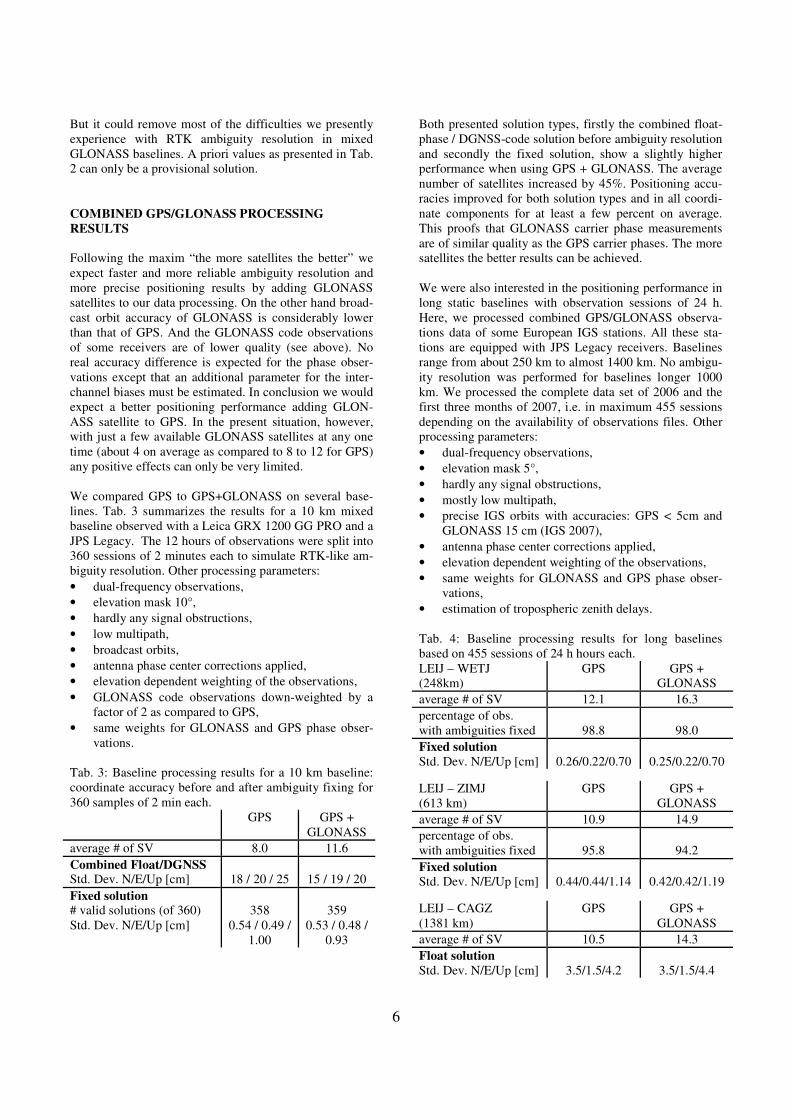
The inter-channel bias differences of a 9 day long experi-
ment are shown in Fig. 5. No effect of the temperature
change can be observed. But the change of antenna and
antenna cables for one of the receivers in order to observe
a zero baseline produced a jump in the Glonasshc δ∆⋅0 time
series. This jump is most striking in the ionosphere-free
linear combination where it amounts to 1.4 mm (Fig. 5).
Fig: 3: Double difference (DD) residuals of two short GPS/GLONASS baselines.
5
Fig. 4: Daily estimates of the inter-channel bias differ-
ences Glonasshc δ∆⋅0 in the short baseline WTZZ (Ashtech
Z-18) and WTZJ (JPS Legacy) at Wettzell, Germany dur-
ing a period of more than one year. Shown are results for
L1, L2, and the ionosphere-free linear combination L0.
Fig. 5: Inter-channel bias differences Glonasshc δ∆⋅0 of two
receivers from different manufacturers before, during, and
after a chilling experiment.
The analysis of the GLONASS observation data in mixed
baselines showed that the inter-channel bias differences Glonasshc δ∆⋅0 can be as large as 2.5 cm. They are esti-
mated from the baseline observations after fixing of the
ambiguities. If these bias differences exceed a few milli-
metres, reliable ambiguity fixing gets much more difficult
or can not be performed at all for positioning techniques
like RTK (Real Time Kinematic). We therefore recom-
mend introducing a priori values of the biases into the
data processing to support ambiguity resolution.
We estimated approximate values Glonasshc δ∆⋅0 from the
observations gathered in short mixed baselines. The cor-
rection values presented in Tab. 2 are only valid for firm-
ware versions of receivers of early 2007. Large changes
of these values may occur if a manufacturer modifies pre-
correction values applied by the receiver firmware. The
accuracies of the values in Tab. 2 are on the level of a few
millimetres. Higher accuracies can not be obtained due to
effects which do not depend on the receiver itself but on
the antenna and antenna cable. We also found that a dis-
tinction of L1 and L2 corrections is not necessary on this
level of accuracy. Hence, Tab. 2 contains a single value
for each receiver pair.
Tab. 2: Estimates of GLONASS inter-channel bias differ-
ences Glonasshc δ∆⋅0 in centimetres for several receiver
pairs.
Ashtech
Z-18
JPS Legacy,
TPS E_GGD,
TPS Net-G3
Leica GRX
1200 GG PRO
Trimble
NetR5
Ashtech
Z-18
0.0 0.0 2.4 -0.7
JPS Legacy,
TPS E_GGD,
TPS Net-G3 0.0 0.0 2.4 -0.7
Leica GRX
1200 GG
PRO
-2.4 -2.4 0.0 -3.1
Trimble
NetR5
0.7 0.7 3.1 0.0
It would be advantageous for all GNSS users if the manu-
facturers of GPS/GLONASS-receivers could agree on a
common level of these inter-channel biases and if they
could apply appropriate corrections to the GLONASS
observations in their receiver firmware. This could, of
course, not completely remove the difficulty of inter-
channel biases in mixed baselines, because part of the
problem is caused by the antennas and antenna cables.
6
But it could remove most of the difficulties we presently
experience with RTK ambiguity resolution in mixed
GLONASS baselines. A priori values as presented in Tab.
2 can only be a provisional solution.
COMBINED GPS/GLONASS PROCESSING
RESULTS
Following the maxim “the more satellites the better” we
expect faster and more reliable ambiguity resolution and
more precise positioning results by adding GLONASS
satellites to our data processing. On the other hand broad-
cast orbit accuracy of GLONASS is considerably lower
than that of GPS. And the GLONASS code observations
of some receivers are of lower quality (see above). No
real accuracy difference is expected for the phase obser-
vations except that an additional parameter for the inter-
channel biases must be estimated. In conclusion we would
expect a better positioning performance adding GLON-
ASS satellite to GPS. In the present situation, however,
with just a few available GLONASS satellites at any one
time (about 4 on average as compared to 8 to 12 for GPS)
any positive effects can only be very limited.
We compared GPS to GPS+GLONASS on several base-
lines. Tab. 3 summarizes the results for a 10 km mixed
baseline observed with a Leica GRX 1200 GG PRO and a
JPS Legacy. The 12 hours of observations were split into
360 sessions of 2 minutes each to simulate RTK-like am-
biguity resolution. Other processing parameters:
• dual-frequency observations,
• elevation mask 10°,
• hardly any signal obstructions,
• low multipath,
• broadcast orbits,
• antenna phase center corrections applied,
• elevation dependent weighting of the observations,
• GLONASS code observations down-weighted by a
factor of 2 as compared to GPS,
• same weights for GLONASS and GPS phase obser-
vations.
Tab. 3: Baseline processing results for a 10 km baseline:
coordinate accuracy before and after ambiguity fixing for
360 samples of 2 min each.
GPS GPS +
GLONASS
average # of SV 8.0 11.6
Combined Float/DGNSS Std. Dev. N/E/Up [cm]
18 / 20 / 25
15 / 19 / 20
Fixed solution # valid solutions (of 360)
Std. Dev. N/E/Up [cm]
358
0.54 / 0.49 /
1.00
359
0.53 / 0.48 /
0.93
Both presented solution types, firstly the combined float-
phase / DGNSS-code solution before ambiguity resolution
and secondly the fixed solution, show a slightly higher
performance when using GPS + GLONASS. The average
number of satellites increased by 45%. Positioning accu-
racies improved for both solution types and in all coordi-
nate components for at least a few percent on average.
This proofs that GLONASS carrier phase measurements
are of similar quality as the GPS carrier phases. The more
satellites the better results can be achieved.
We were also interested in the positioning performance in
long static baselines with observation sessions of 24 h.
Here, we processed combined GPS/GLONASS observa-
tions data of some European IGS stations. All these sta-
tions are equipped with JPS Legacy receivers. Baselines
range from about 250 km to almost 1400 km. No ambigu-
ity resolution was performed for baselines longer 1000
km. We processed the complete data set of 2006 and the
first three months of 2007, i.e. in maximum 455 sessions
depending on the availability of observations files. Other
processing parameters:
• dual-frequency observations,
• elevation mask 5°,
• hardly any signal obstructions,
• mostly low multipath,
• precise IGS orbits with accuracies: GPS < 5cm and
GLONASS 15 cm (IGS 2007),
• antenna phase center corrections applied,
• elevation dependent weighting of the observations,
• same weights for GLONASS and GPS phase obser-
vations,
• estimation of tropospheric zenith delays.
Tab. 4: Baseline processing results for long baselines
based on 455 sessions of 24 h hours each.
LEIJ – WETJ
(248km)
GPS GPS +
GLONASS
average # of SV 12.1 16.3
percentage of obs.
with ambiguities fixed
98.8
98.0
Fixed solution
Std. Dev. N/E/Up [cm]
0.26/0.22/0.70
0.25/0.22/0.70
LEIJ – ZIMJ
(613 km)
GPS GPS +
GLONASS
average # of SV 10.9 14.9
percentage of obs.
with ambiguities fixed
95.8
94.2
Fixed solution
Std. Dev. N/E/Up [cm]
0.44/0.44/1.14
0.42/0.42/1.19
LEIJ – CAGZ
(1381 km)
GPS GPS +
GLONASS
average # of SV 10.5 14.3
Float solution
Std. Dev. N/E/Up [cm]
3.5/1.5/4.2
3.5/1.5/4.4
7
For some baselines, we removed a seasonal trend in the
coordinate time series before calculating standard devia-
tions. The results (Tab. 4) show that, although the average
number of satellite signals increased by more than 35 %,
no overall improvement in coordinate accuracy could be
achieved. One reason may be found in the lower accuracy
of precise IGS GLONASS orbits (15 cm) as compared to
IGS GPS final orbits (<5 cm) which results in lower
weights for GLONASS observations as compared to GPS
observations.
SBAS SATELLITES AND OBSERVATION EQUA-
TION
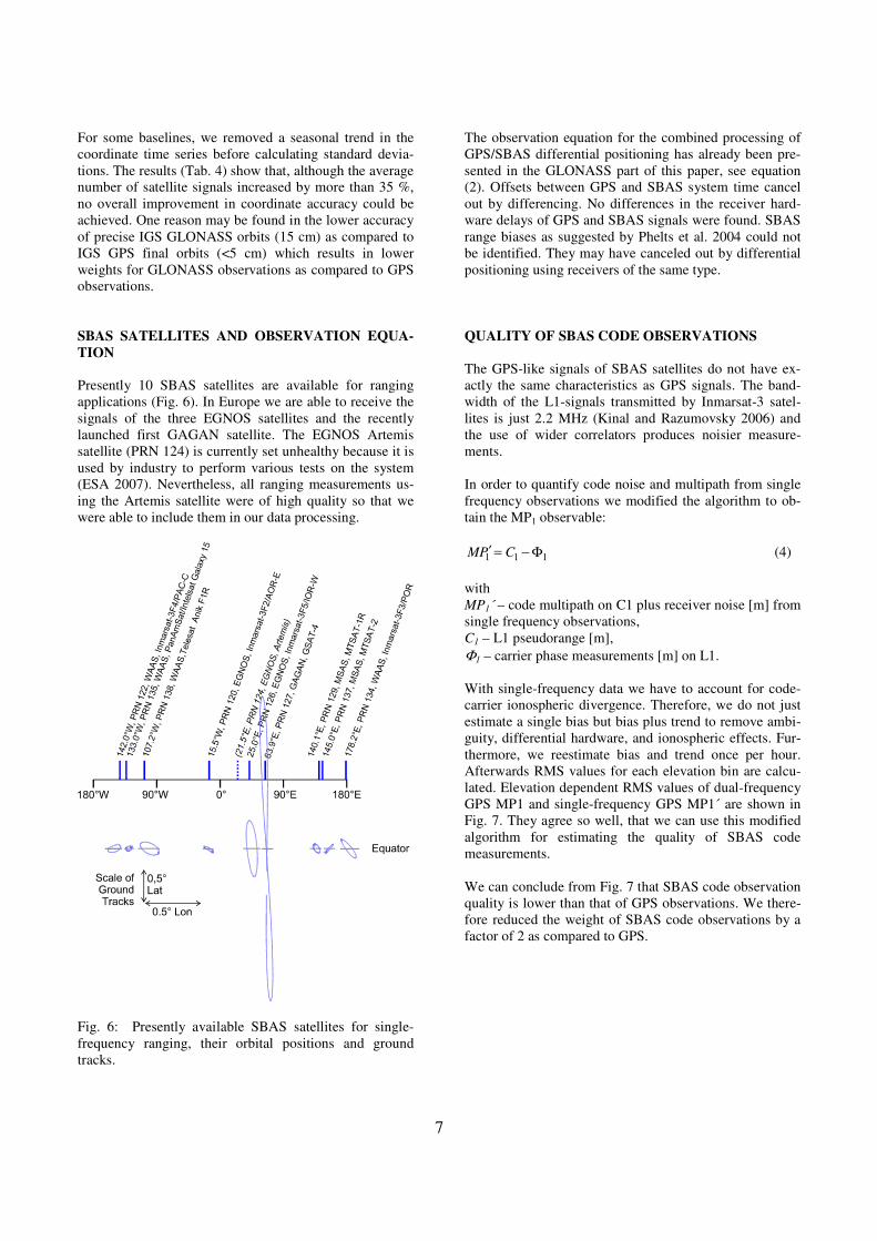
Presently 10 SBAS satellites are available for ranging
applications (Fig. 6). In Europe we are able to receive the
signals of the three EGNOS satellites and the recently
launched first GAGAN satellite. The EGNOS Artemis
satellite (PRN 124) is currently set unhealthy because it is
used by industry to perform various tests on the system
(ESA 2007). Nevertheless, all ranging measurements us-
ing the Artemis satellite were of high quality so that we
were able to include them in our data processing.
Fig. 6: Presently available SBAS satellites for single-
frequency ranging, their orbital positions and ground
tracks.
The observation equation for the combined processing of
GPS/SBAS differential positioning has already been pre-
sented in the GLONASS part of this paper, see equation
(2). Offsets between GPS and SBAS system time cancel
out by differencing. No differences in the receiver hard-
ware delays of GPS and SBAS signals were found. SBAS
range biases as suggested by Phelts et al. 2004 could not
be identified. They may have canceled out by differential
positioning using receivers of the same type.
QUALITY OF SBAS CODE OBSERVATIONS
The GPS-like signals of SBAS satellites do not have ex-
actly the same characteristics as GPS signals. The band-
width of the L1-signals transmitted by Inmarsat-3 satel-
lites is just 2.2 MHz (Kinal and Razumovsky 2006) and
the use of wider correlators produces noisier measure-
ments.
In order to quantify code noise and multipath from single
frequency observations we modified the algorithm to ob-
tain the MP1 observable:
111 Φ−=′ CPM (4)
with
MP1´ – code multipath on C1 plus receiver noise [m] from
single frequency observations,
C1 – L1 pseudorange [m],
Φ1 – carrier phase measurements [m] on L1.
With single-frequency data we have to account for code-
carrier ionospheric divergence. Therefore, we do not just
estimate a single bias but bias plus trend to remove ambi-
guity, differential hardware, and ionospheric effects. Fur-
thermore, we reestimate bias and trend once per hour.
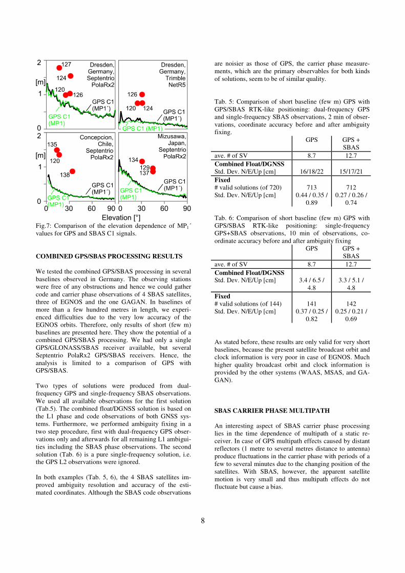
Afterwards RMS values for each elevation bin are calcu-
lated. Elevation dependent RMS values of dual-frequency
GPS MP1 and single-frequency GPS MP1´ are shown in
Fig. 7. They agree so well, that we can use this modified
algorithm for estimating the quality of SBAS code
measurements.
We can conclude from Fig. 7 that SBAS code observation
quality is lower than that of GPS observations. We there-
fore reduced the weight of SBAS code observations by a
factor of 2 as compared to GPS.
8
Fig.7: Comparison of the elevation dependence of MP1´
values for GPS and SBAS C1 signals.
COMBINED GPS/SBAS PROCESSING RESULTS
We tested the combined GPS/SBAS processing in several
baselines observed in Germany. The observing stations
were free of any obstructions and hence we could gather
code and carrier phase observations of 4 SBAS satellites,
three of EGNOS and the one GAGAN. In baselines of
more than a few hundred metres in length, we experi-
enced difficulties due to the very low accuracy of the
EGNOS orbits. Therefore, only results of short (few m)
baselines are presented here. They show the potential of a
combined GPS/SBAS processing. We had only a single
GPS/GLONASS/SBAS receiver available, but several
Septentrio PolaRx2 GPS/SBAS receivers. Hence, the
analysis is limited to a comparison of GPS with
GPS/SBAS.
Two types of solutions were produced from dual-
frequency GPS and single-frequency SBAS observations.
We used all available observations for the first solution
(Tab.5). The combined float/DGNSS solution is based on
the L1 phase and code observations of both GNSS sys-
tems. Furthermore, we performed ambiguity fixing in a
two step procedure, first with dual-frequency GPS obser-
vations only and afterwards for all remaining L1 ambigui-
ties including the SBAS phase observations. The second
solution (Tab. 6) is a pure single-frequency solution, i.e.
the GPS L2 observations were ignored.
In both examples (Tab. 5, 6), the 4 SBAS satellites im-
proved ambiguity resolution and accuracy of the esti-
mated coordinates. Although the SBAS code observations
are noisier as those of GPS, the carrier phase measure-
ments, which are the primary observables for both kinds
of solutions, seem to be of similar quality.
Tab. 5: Comparison of short baseline (few m) GPS with
GPS/SBAS RTK-like positioning: dual-frequency GPS
and single-frequency SBAS observations, 2 min of obser-
vations, coordinate accuracy before and after ambiguity
fixing.
GPS GPS +
SBAS
ave. # of SV 8.7 12.7
Combined Float/DGNSS
Std. Dev. N/E/Up [cm]
16/18/22
15/17/21
Fixed
# valid solutions (of 720)
Std. Dev. N/E/Up [cm]
713
0.44 / 0.35 /
0.89
712
0.27 / 0.26 /
0.74
Tab. 6: Comparison of short baseline (few m) GPS with
GPS/SBAS RTK-like positioning: single-frequency
GPS+SBAS observations, 10 min of observations, co-
ordinate accuracy before and after ambiguity fixing
GPS GPS +
SBAS
ave. # of SV 8.7 12.7
Combined Float/DGNSS Std. Dev. N/E/Up [cm]
3.4 / 6.5 /
4.8
3.3 / 5.1 /
4.8
Fixed
# valid solutions (of 144)
Std. Dev. N/E/Up [cm]
141
0.37 / 0.25 /
0.82
142
0.25 / 0.21 /
0.69
As stated before, these results are only valid for very short
baselines, because the present satellite broadcast orbit and
clock information is very poor in case of EGNOS. Much
higher quality broadcast orbit and clock information is
provided by the other systems (WAAS, MSAS, and GA-
GAN).
SBAS CARRIER PHASE MULTIPATH
An interesting aspect of SBAS carrier phase processing
lies in the time dependence of multipath of a static re-
ceiver. In case of GPS multipath effects caused by distant
reflectors (1 metre to several metres distance to antenna)
produce fluctuations in the carrier phase with periods of a
few to several minutes due to the changing position of the
satellites. With SBAS, however, the apparent satellite
motion is very small and thus multipath effects do not
fluctuate but cause a bias.
9
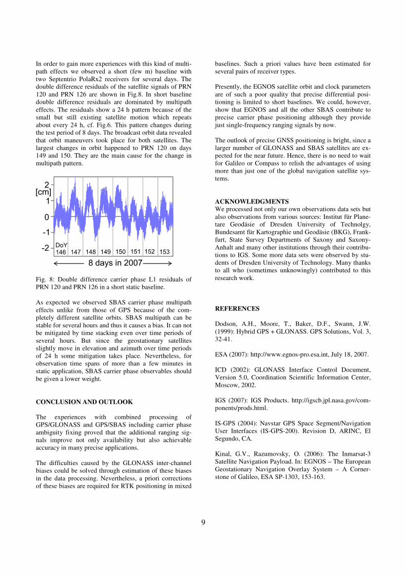
In order to gain more experiences with this kind of multi-
path effects we observed a short (few m) baseline with
two Septentrio PolaRx2 receivers for several days. The
double difference residuals of the satellite signals of PRN
120 and PRN 126 are shown in Fig.8. In short baseline
double difference residuals are dominated by multipath
effects. The residuals show a 24 h pattern because of the
small but still existing satellite motion which repeats
about every 24 h, cf. Fig.6. This pattern changes during
the test period of 8 days. The broadcast orbit data revealed
that orbit maneuvers took place for both satellites. The
largest changes in orbit happened to PRN 120 on days
149 and 150. They are the main cause for the change in
multipath pattern.
Fig. 8: Double difference carrier phase L1 residuals of
PRN 120 and PRN 126 in a short static baseline.
As expected we observed SBAS carrier phase multipath
effects unlike from those of GPS because of the com-
pletely different satellite orbits. SBAS multipath can be
stable for several hours and thus it causes a bias. It can not
be mitigated by time stacking even over time periods of
several hours. But since the geostationary satellites
slightly move in elevation and azimuth over time periods
of 24 h some mitigation takes place. Nevertheless, for
observation time spans of more than a few minutes in
static application, SBAS carrier phase observables should
be given a lower weight.
CONCLUSION AND OUTLOOK
The experiences with combined processing of
GPS/GLONASS and GPS/SBAS including carrier phase
ambiguity fixing proved that the additional ranging sig-
nals improve not only availability but also achievable
accuracy in many precise applications.
The difficulties caused by the GLONASS inter-channel
biases could be solved through estimation of these biases
in the data processing. Nevertheless, a priori corrections
of these biases are required for RTK positioning in mixed
baselines. Such a priori values have been estimated for
several pairs of receiver types.
Presently, the EGNOS satellite orbit and clock parameters
are of such a poor quality that precise differential posi-
tioning is limited to short baselines. We could, however,
show that EGNOS and all the other SBAS contribute to
precise carrier phase positioning although they provide
just single-frequency ranging signals by now.
The outlook of precise GNSS positioning is bright, since a
larger number of GLONASS and SBAS satellites are ex-
pected for the near future. Hence, there is no need to wait
for Galileo or Compass to relish the advantages of using
more than just one of the global navigation satellite sys-
tems.
ACKNOWLEDGMENTS
We processed not only our own observations data sets but
also observations from various sources: Institut für Plane-
tare Geodäsie of Dresden University of Technolgy,
Bundesamt für Kartographie und Geodäsie (BKG), Frank-
furt, State Survey Departments of Saxony and Saxony-
Anhalt and many other institutions through their contribu-
tions to IGS. Some more data sets were observed by stu-
dents of Dresden University of Technology. Many thanks
to all who (sometimes unknowingly) contributed to this
research work.
REFERENCES
Dodson, A.H., Moore, T., Baker, D.F., Swann, J.W.
(1999): Hybrid GPS + GLONASS. GPS Solutions, Vol. 3,
32-41.
ESA (2007): http://www.egnos-pro.esa.int, July 18, 2007.
ICD (2002): GLONASS Interface Control Document,
Version 5.0, Coordination Scientific Information Center,
Moscow, 2002.
IGS (2007): IGS Products. http://igscb.jpl.nasa.gov/com-
ponents/prods.html.
IS-GPS (2004): Navstar GPS Space Segment/Navigation
User Interfaces (IS-GPS-200). Revision D, ARINC, El
Segundo, CA.
Kinal, G.V., Razumovsky, O. (2006): The Inmarsat-3
Satellite Navigation Payload. In: EGNOS – The European
Geostationary Navigation Overlay System – A Corner-
stone of Galileo, ESA SP-1303, 153-163.
10
Phelts, R.E., Walter, T., Enge, P., Akos, D.M., Shallberg,
K., Morrissey, T. (2004): Range Biases on the WAAS
Geostationary Satellites. ION NTM 2004, 110-120.
Pratt, M., Burke, B., Misra, P. (1998): Single-Epoch Inte-
ger Ambiguity Resolution with GPS-GLONASS L1-L2
Data. Proc. ION GPS-98, 389-398.
Rocken, C., Meertens, C., Stephens, B., Braun, J., Van-
Hove, T., Perry, S., Ruud, O., McCallum, M., Richardson,
J. (1995): UNAVCO Academic Research Infrastructure
Receiver and Antenna Test Report. UNVACO, Boulder
CO, November 1995.
Soddu, C., Van Dierendonck, A.J., Secretan, H., Ventura-
Traveset, J., Dusseauze, P.-Y., Pasquali, R. (2005): In-
marsat-4 First L1/L5 Satellite: Preparing for SBAS L5
Service. Proc. ION GNSS 2005, 2304-2315.
Ventura-Traveset, J., Gauthier, L., Toran, F., Michel, P.,
Solari, G., Salabert, F., Flament, D., Auroy, J., Beaugnon,
D. (2006): The European EGNOS Project : Mission, Pro-
gramme and System. In: EGNOS – The European Geosta-
tionary Navigation Overlay System – A Cornerstone of
Galileo, ESA SP-1303, 3-19.
Zinoviev, A.E. (2005): Using GLONASS in Combined
GNSS Receivers: Current Status. Proc. ION GNSS 2005,
1046-1057.


![Phase Vocoder Colter McQuay Phase Vocoder Structure Input x[nTs] Effect Specific Code Synthesize Output y[nTs] Analyze](https://cdn.vdocuments.net/doc/165x107/56649d2d5503460f94a0489e/phase-vocoder-colter-mcquay-phase-vocoder-structure-input-xnts-effect-specific.jpg)
