
1
Computation of Weakly-Compressible
Highly-Viscous Polymeric Liquid Flows
M. F. Webster 1* , I. J. Keshtiban 2, and F. Belblidia 1
(1) Institute of Non-Newtonian Fluid Mechanics,
Department of Computer Science,
University of Wales, Swansea, SA2 8PP, UK.
(2) Research visitor, Tarbiat Modares University of Teheran, Iran.
* Author for correspondence. Email: [email protected]
2
Abstract
We introduce a high-resolution time-marching pressure-correction algorithm to
accommodate weakly-compressible highly-viscous polymeric liquid flows at low Mach
number. As the incompressible limit is approached ( 0≈Ma ), the consistency of the
compressible scheme is highlighted in recovering equivalent incompressible solutions. In
the viscous-dominated regime of low Reynolds number (zone of interest), the algorithm
treats the viscous part of the equations in a semi-implicit form. Two discrete
representations are proposed to interpolate density: a piecewise-constant form with
gradient recovery and a linear interpolation form, akin to that on pressure. Numerical
performance is considered on a number of classical benchmark problems for viscous
polymeric liquid flows to highlight consistency, accuracy and stability properties.
Validation bears out the high quality of performance of both compressible flow
implementations, at low to vanishing Mach number. Neither linear, nor constant density
interpolations schemes degrade the second-order accuracy of the original incompressible
fractional-staged pressure-correction scheme. The piecewise-constant interpolation scheme
is advocated strongly as the preferred method of choice, with its advantages of order
retention, yet efficiency in implementation.
Key Words: Finite element, pressure-correction, highly-viscous, polymeric-liquid, compressible
flow, low Mach number.

3
1. INTRODUCTION
This article addresses the need to predict solutions for weakly-compressible highly-
viscous polymeric liquid flows, with attention to both accuracy and efficiency. The
approach commences from a framework adopted for incompressible flow and viscoelastic
fluids, upon which compressibility is grafted. Here, viscous Newtonian fluids are
considered, so that inertial effects are low to moderate, yet viscosities may be high. In such
a context, the level of corresponding Reynolds number is low (typically, ( )1Re O≈ ),
diffusion dominates and convection terms may be resolved without difficulty. This lies in
contrast to the aerodynamic high-convection regime (inertial, low-viscosity, high-speed),
which gives rise to shocks and where characteristic-based methods are relevant. Here, such
issues do not emerge. Furthermore, our ultimate goal is to address viscoelastic flows, where
convection of stress (fluid-memory) is important, that does demand a suitable form of
upwinding, see Petrov-Galerkin forms (Matallah et al., 1998).
Compressibility effects occur in both liquids and gases through the variation of density.
Density itself, depends on temperature, pressure and concentration levels. Flows of liquid
materials, at moderate pressure levels, can be considered as incompressible. Nevertheless,
at large pressure-differences, such flows may display some mild compressibility effects.
Mach number, the ratio of fluid velocity to the speed of sound ( cuMa /= ), characterises
the influence of compressibility on a flow field. Flows at low Mach number may be
described as incompressible, whilst for those at moderate to high Mach number,
compressibility effects will be prominent. The incompressible limit of a compressible flow
is approached, under suitable constraints, as Mach number vanishes (Munz et al., 2003).
Under such circumstances, the speed of sound is much larger than the velocity of the
liquid, resulting in fast pressure waves, where rapid pressure equalization takes place.

4
Low Mach number flows play an important role, occurring widely in nature and
industrial processes. Circulation within the oceans is driven mainly by density gradients,
which arise via variation of salinity and temperature. Common human bodily functions,
such as, singing, weaseling, breathing and talking, all represent examples of low Mach
number flow regimes. In addition, some industrial gas flow configurations take place at
low Mach number. Free convection and combustion are yet further examples, where flow
occurs driven under the variation of density with temperature. Compressibility has some
impact upon applications such as in: liquid impact, jet cutting and liquid impact erosion, in
steam turbine for example (Kelmanson and Maunder, 1999, Field, 1999); polymer
extrusion (Georgiou, 2003); injection molding with polymer melts (Han and Im, 1997);
recovery and exploration of petroleum (Wu and Pruess, 2000). Compressibility should be
incorporated in order to rigorously investigate such phenomena as cavitation (Brujan,
1999), instabilities (Georgiou, 2003), and shrinkage and warpage (Han and Im, 1997),
liquid impact erosion (Kelmanson and Maunder, 1999, Jackson and Field, 1999).
Moreover, in capillary rheometry, compressibility may have a significant influence on
features such as the time-dependent pressure changes within a system (see piston-driven
flows, Ranganathan et al., 1999)
Much attention has been devoted towards the computational solution of flows that
manifest compressibility effects. Today, sophisticated numerical solvers can handle high
Reynolds number compressible flow computations. To solve such scenarios, different
methodologies have emerged under finite element and finite volume approaches. Within
finite elements, this gives rise to various Streamline-Upwind/Petrov-Galerkin (SUPG)
algorithms, with stabilization techniques such as Galerkin Least-Square (GLS) (Hughes et
al., 1989). Equivalently, in the finite volume context, some high-performance counterpart
algorithms have emerged (Moukalled and Darwish, 2001, Karki and Patankar, 1989,

5
Karimian and Schneider, 1995). Nonetheless, Wong et al. (2001), state that some SUPG
compressible-based algorithms may fail to yield adequate numerical solutions for flows
that approach the incompressible limit. Degradation in the solution has been observed in
several studies (Turkel et al., 1997, Wong et al., 2001). One of the key difficulties in
constructing numerical methods to address weakly-compressible flows arises from the fact
that the governing equations switch type. The equations for viscous compressible flow
form a hyperbolic-parabolic system with finite waves-speeds (invisid case, hyperbolic),
whilst those for incompressible viscous flow assume an elliptic-parabolic system with
infinite wave propagation rates (for viscoelastic regimes, a sub-system of hyperbolic form
may augment the whole). In addition, the compressible equations for low Mach number
may be associated with large disparity between the acoustic wave-speed, (u + c), and the
entropy wave convected at the fluid-speed, (u) (Wong et al., 2001, Turkel et al., 1997,
Jenny and Muller, 1999). Here, the condition number for the equation system is related to
the reciprocal of the Mach number.
In the present article under algorithmic development, we restrict ourselves to Newtonian
viscous polymeric liquid flows under isothermal conditions and where Reynolds and Mach
numbers are generally low (viscoelastic alternatives to follow). An equation of state is
applied to represent density variation with pressure. To this end the well-established Tait
model (Tait, 1888) is suitably extended, chosen on physical ground to represent polymeric
materials (Huang and Chow, 1974, Han and Im, 1997). Key modifications to handle
weakly-compressible flows, introduced within our fractional-staged incompressible
pressure-correction algorithm, are related primarily to the finite element representation of
density. Two types of interpolation are employed: first, a piecewise-constant form
(incompressible per element), with a nodal recovery for density gradients (second-stage);
second, a linear interpolation form, akin to that employed for the pressure field. We

6
demonstrate that these modifications do not degrade second-order accuracy of the original
pressure-correction scheme. We illustrate how the algorithm can handle weakly-
compressible highly-viscous flow at low Mach number, as well as incompressible flows
(hence, zero Mach number configurations).
The present article is organized as follows: background theory is introduced in Section
2. The governing equations for compressible viscous flows are expounded in Section 3. In
Section 4, we introduce the equation stages in the scheme, followed in Section 5 by the
finite element (FE) discretisation adopted. In Section 6, we present the application of our
methodology to several benchmark test-problems, including driven-cavity flows, channel
flows and contraction flows. Scheme variants are validated for consistency via mesh
refinement, to extract respective orders of accuracy. Comparison, is made against
incompressible counterparts and the literature, complementing the high-order of accuracy
achieved. This proves itself above second-order for smooth flows. The piecewise-constant
interpolation scheme is advocated strongly on a number of counts, as outlined below.
2. BACKGROUND THEORY
The need for algorithmic developments to handle the low Mach number flow regime
may be justified on a number of grounds. For example, there are many natural phenomena,
where accurate simulation in this scenario is demanded. In some instances, flow problems
may exhibit mixed-type (compressible/incompressible), where some sections of the flow
are incompressible with locally low Mach number, whilst other zones are significantly
compressible. Under such circumstances, if the incompressible region is sufficiently small,
compared to the compressible section, there is little loss of accuracy when
incompressibility is neglected. However, there are flow regimes, such as in aerodynamics
(high-speed/low-viscosity), where large regions of low Mach number coexist alongside

7
supersonic flow regions. This arises in aerofoil high angle-of-attack configurations, where
the solution will degrade if based solely on a compressible description. In addition, in some
material processing instances, such as for polymers during the filling stage of injection
moulding and in extrusion, there are some locally compressible regions, whilst most of the
flow remains incompressible. Therefore, it is both desirable and necessary to develop
algorithms that can handle both regimes, concurrently. From a numerical perspective,
conventional approaches to handle low Mach number flows can be subjugated into two
main categories: density-based schemes and pressure-based schemes (Moukalled and
Darwish, 2001, Karki and Patankar, 1989). We proceed to follow the latter, upon which the
present article is based.
Density-based methods represent a large class of schemes adopted for compressible
flows (for more details see, Keshtiban et al., 2003). Turkel et al. (1997) and Guillard and
Viozat (1999) have identified that, in the low Mach number limit, the discretised solution
of the compressible flow equations may fail to provide an accurate approximation to the
incompressible equations (quoting Guillard and Viozat (1999) in particular). As a ‘rule-of-
thumb’, compressible schemes without modification become impractical for Mach
numbers lower than around 0.3 (Roller and Munz, 2000). In contrast, pressure-based
methods were originally conceived to solve incompressible flows, adopting pressure as a
primary variable. With this approach, pressure variation remains finite, irrespective of
Mach number, rendering computation tractable throughout the entire spectrum of Mach
number (Karki and Patankar, 1989), hence circumventing the shortcomings of density-
based methods. The first implementation of pressure-based schemes for compressible flow
is widely attributed to the early contribution of Harlow and Amsden (1968), based on a
semi-implicit finite difference algorithm.

8
Pressure-correction, or projection methods, are pressure-based fractional-staged
schemes with correction for velocity and pressure (see Peyret and Taylor, 1983),
introduced through the pioneering work of Chorin (1968) and Temam (1969). Such
methods have been employed effectively within several finite volume implementations,
say through the SIMPLE (Semi-Implicit Pressure Linked Equations) family of schemes
(Patankar, 1980). Karki and Patankar (1989) developed the SIMPLER method for
compressible flows, applicable for a wide range of problem-speeds. These SIMPLE
methods are first-order in time. Munz et al. (2003) extended the SIMPLE scheme for low
Mach number flow employing multiple pressure variables, each being associated with
different physical response. Similar procedures have been adopted by others (Bijl and
Wesseling, 1998, Mary et al., 2000, Roller and Munz, 2000). Pressure-correction was
taken forward within finite differences to a second-order by Van Kan (1986).
Alternatively, within finite elements, Donea et al. (1982) introduced a pressure-correction
fractional-step method, designed to significantly reduce computational overheads in
transient incompressible viscous flow situations. Similarly, Zienkiewicz et al. (1995) have
introduced the characteristic-based-split procedure (CBS). This implementation is a
Taylor-Galerkin/Pressure-Correction scheme, suitable for both incompressible and
compressible flow regimes. The crux here, is to split the equation system into two parts: a
part of convection-diffusion type (discretised via a characteristic-Galerkin procedure) and
one of self-adjoint type. With the characteristic-based-split scheme, one may solve both
parts of the system in an explicit manner. Alternatively, one may use a semi-implicit
scheme for the first part, allowing for much larger time-steps, and solve the second part
implicitly, with its advantage of unconditional stability. The characteristic-based-split
procedure has been tested successfully on a number of scenarios, for example, transonic
9
and supersonic flows, low Mach number flows with low and high viscosity, and in
addition, on shallow-water wave problems.
In the incompressible viscoelastic regime, computational methods have matured
significantly over the last two decades or so (Saramito and Piau, 1994, Guénette and
Fortin, 1995, Baaijens, 1998, Walters and Webster, 2003). Here, it is desirable to extend
the methodology into the weakly-compressible regime, and particularly so for viscous
polymeric liquid flows. In this regard, density-based preconditioning or asymptotic
methods (see Keshtiban et al., 2003) often demand significant recoding. On the other
hand, extending an existing incompressible flow code to accommodate compressibility
would appear somewhat more straightforward. This is the thesis and starting point adopted
for implementation throughout the current study. Precisely, our aim is to modify a
pressure-correction technique for incompressible polymeric flows to accommodate
weakly-compressible, yet highly-viscous, flows under low Mach number configurations.
This presents a natural extension to our earlier incompressible flow studies for viscous
(Hawken et al., 1990), inelastic (Ding et al., 1995, three-dimensional) and viscoelastic
(Matallah et al., 1998, Wapperom and Webster, 1998) fluids, where we have developed a
hybrid schema to attain second-order accuracy.
3. GOVERNING EQUATIONS
The conservation of mass and momentum transport equations employed in the
simulation of compressible steady Newtonian fluid under isothermal conditions may be
considered as:
0).( =∇+∂∂
ut
ρρ (1)
]..[ puut
u ∇−∇−∇=∂∂ ρτρ (2)

10
where independent variables are (t,x), time and space, and dependent field variables are ρ ,
u, τ , p, density, velocity, stress and pressure, respectively. Stress is related to the
kinematic field through a constitutive law, which is defined for compressible Newtonian
fluids as: ( )
⋅∇−= ijijij ud δµτ3
2 (3)
where µ is the viscosity, ijδ is the Kronecker delta tensor and Tuud ∇+∇=2 is the rate of
deformation tensor (here, superscript T denotes tensor transpose).
To extract non-dimensionalised governing equations, we define the following scales on
physical variables as: velocityoU , dimension L, density oρ , pressure and stress
L
Uoµand
time oU
L. We introduce the dimensionless group Reynolds number,
µρ LU oo=Re , to
extract the non-dimensionalised momentum equation:
puut
u ∇−∇⋅−∇=∂∂ ρτρ Re.Re . (4)
Correspondence in the continuity equation provides:
0).( =∇+∂∂
ut
ρρ. (5)
To complete the set of governing equations, it is necessary to introduce an equation of
state relating density to pressure. For polymeric liquids, we consider the modified Tait
equation of state (Tait, 1888), in the form
m
Bp
Bp
=
++
00 ρρ
, (6)
where, m and B are parameters and op , oρ denote reference values for pressure and
density, respectively. This empirical equation of state is suitable for dense materials, such
as polymer melts and solutions, water and other liquids (Huang and Chow, 1974, under

11
linear approximation (m=1), see also, Ranganathan et al., 1999, and Georgiou, 2003).
Note, that strictly speaking, this equation applies only to isentropic change. Nevertheless, it
can be utilise with reasonable accuracy in more general instances, since m and B are
independent of entropy and oρ is constant (Brujan, 1999). We follow Karki and Patankar
(1989), Zienkiewicz et al. (1995) and Brujan (1999), and after differentiating the equation
of state, we gather:
2),(
1 )(txc
Bpmmk
P m =+==∂∂ −
ρρ
ρ (7)
where ( )
mo Bp
k0ρ+= is a constant and c(x,t) is the derived speed of sound, a field parameter
distributed in space x and time t. Other alternatives assumptions may be adopted, such as
isenthalpic (Lien and Leschziner, 1993) or homenthalpic (Munz et al., 2003). Note, under
steady-state conditions, temporal pressure change will vanish and the steady solution will
be independent of the above stated assumptions. However, this may affect transient results
and convergence properties of the associated schemes. The next step is to incorporate the
above theory within a discrete representation.
4. PRESSURE-CORRECTION SCHEME - COMPRESSIBLE FLOWS
Recently, we have advocated various advances in the application of our incompressible
second-order, fractional-staged, time-marching pressure-correction procedures. This has
accommodated model to complex flows exemplified through free-surface flows
(Ngamaramvaranggul and Webster, 2000a), wire-coating (Ngamaramvaranggul and
Webster, 2000b) and dough mixing applications (Baloch et al., 2002). Our present goal is
to elaborate the constructive steps to incorporate weak-compressibility upon such a

12
formulation, where we have polymeric liquid flow applications firmly in mind (viscous
form, viscoelastic to follow).
The base formulation-framework is that of a pressure-correction scheme, split into three
distinct, fractional-stages. Briefly, at a first stage, which is divided into two sub-stages, the
momentum equation is employed to predict the velocity field at a half-stage. Subsequently,
the momentum equation is employed to compute the velocity (u*) at a full-step (two-step
Lax-Wendroff style, Taylor-Galerkin phase, (Löhner et al., 1984). The second stage
(pressure-correction) utilises the continuity equation to evaluate a temporal pressure-
difference, inserting the approximate velocity field (auxiliary variable, u*, computed at
stage one). Crank-Nicolson averaged treatment for diffusion/source term introduces semi-
implicitness to the stages and overcomes restrictive diffusive stability limitations. At a
third stage, the end-of-step velocity field (un+1) is corrected, based upon the pressure-
difference on the time-step, derived at the second stage. One may draw distinction to the
characteristic-based-split procedure of Zienkiewicz et al. (1995), in the retention of
pressure gradients, within the representation of the momentum equation over stage one.
This ensures solution at stage two for temporal pressure increments, delivering second-
order accuracy to the system and aiding the appropriate setting of boundary conditions
throughout. The characteristic-based-split approach, alternatively, conveys the pressure
gradient term to the third fractional-staged equation for velocity-correction.
To extend the incompressible algorithm to deal with compressible flows, one must
first appreciate the key role that pressure plays in a compressible flow. In the low Mach
number limit, where density is almost constant, the role of pressure is to influence velocity
through the continuity equation, so that conservation of mass is satisfied (Moukalled and
Darwish, 2001). Indeed, in this instance, density and pressure are only weakly-linked
variables. To recast the above incompressible scheme into one appropriate for weakly-
13
compressible highly-viscous flows, we follow the ideas of Karki and Patankar (1989) and
Zienkiewicz et al. (1995). Here, the temporal derivative of density from the continuity
equation is replaced by its equivalent in pressure, appealing to an equation of state. To
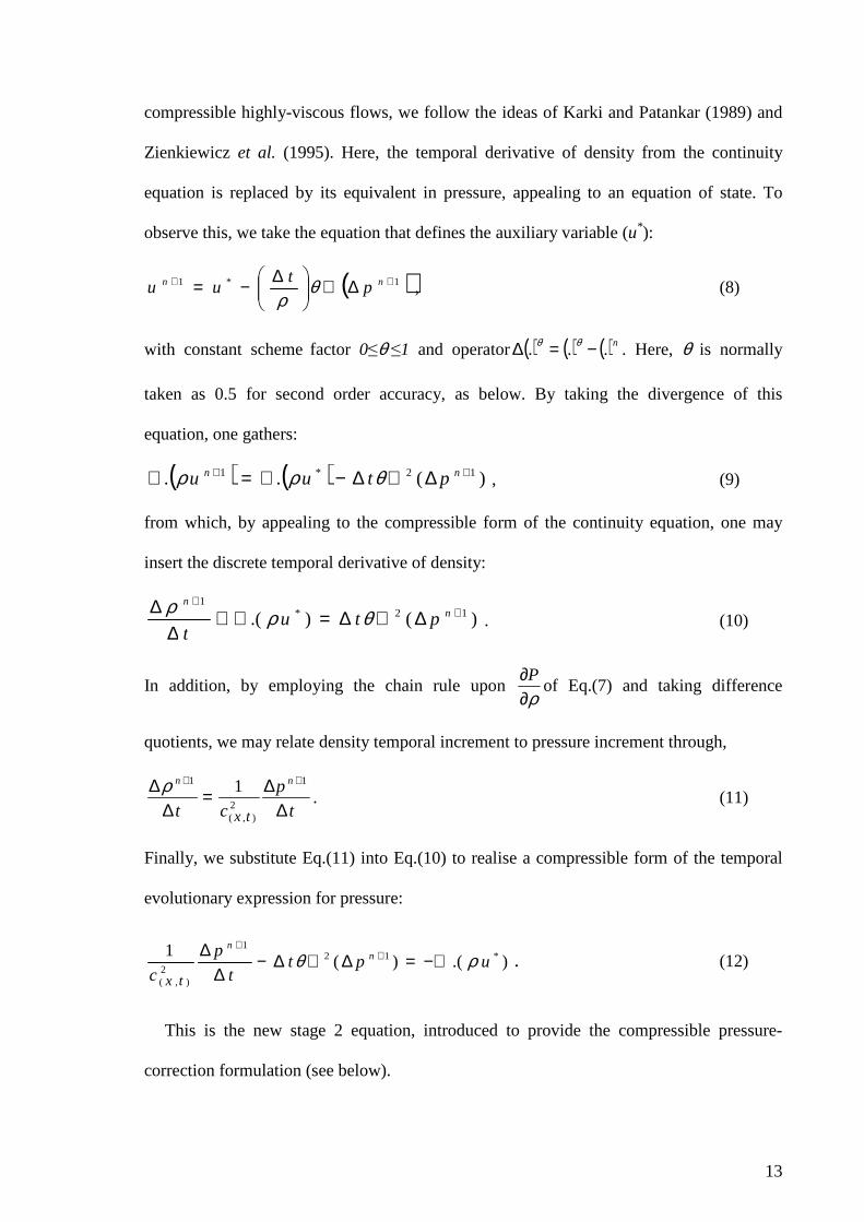
observe this, we take the equation that defines the auxiliary variable (u*):
( )1*1 ++ ∆∇
∆−= nn pt
uu θρ
, (8)
with constant scheme factor 0≤θ ≤1 and operator ( ) ( ) ( )n... −=∆ θθ . Here, θ is normally
taken as 0.5 for second order accuracy, as below. By taking the divergence of this
equation, one gathers:
( ) ( ) )(.. 12*1 ++ ∆∇∆−∇=∇ nn ptuu θρρ , (9)
from which, by appealing to the compressible form of the continuity equation, one may
insert the discrete temporal derivative of density:
)().( 12*1
++
∆∇∆=∇+∆
∆ nn
ptut
θρρ. (10)
In addition, by employing the chain rule upon ρ∂
∂Pof Eq.(7) and taking difference
quotients, we may relate density temporal increment to pressure increment through,
t
p
ct
nn
tx ∆∆=
∆∆ ++ 1
2),(
1 1ρ. (11)
Finally, we substitute Eq.(11) into Eq.(10) to realise a compressible form of the temporal
evolutionary expression for pressure:
).()(1 *12
1
2),(
uptt
p
cn
n
txρθ −∇=∆∇∆−
∆∆ +
+
. (12)
This is the new stage 2 equation, introduced to provide the compressible pressure-
correction formulation (see below).

14
5. FINITE ELEMENT DISCRETIZATION
The momentum and mass conservation equations are discretised via the FE method.
Based on a triangular mesh, the velocity vector ),( txu , and pressure ),( txp are taken over
elements as:
)()(),( xtUtxu jj φ= , j=1,6 and )()(),( xtPtxp kk ψ= , k=1,3 (13)
where
( )xφ represents continuous quadratic polynomial interpolation, ( )xψ piecewise-
linear interpolation, and time-dependent nodal velocity and pressure vectors are U and P,
respectively. We note in the context of highly-viscous polymeric flows, velocity gradients
are a dominant feature and their accurate prediction, via higher-order levels of
interpolation on velocity, are a well-established characteristic of such scenarios. For
density interpolation, two types of interpolation are considered: piecewise-constant over an
element, with recovery for the gradient of density, and piecewise-linear interpolation (as
for the pressure field). The semi-implicit discretised equations for the compressible
pressure-correction scheme may be expressed in three fractional stages:
Stage 1a: [ ]nTU
n
U PLUUNUSUSt
M−+−=
∆
+
∆+
)(2
1
2/2
1
ρρ
(14)
Stage 1b: ( ) [ ] [ ] 2
1* )(
2
1 +−−−=∆
+
∆nnT
UU UUNPLUSUSt
Mρ
ρ (15)
Stage 2: ( ) *12
1UL
tPK
tnC ρθ
∆−=∆
+∆Μ + (16)
Stage 3: ( ) 1*11 ++ ∆=−∆
nTn PLUUMt
θρ (17)
where, in the case of a planar coordinate system, matrix notation implies:

15
( ) Ω= ∫Ω
dM jiijφφρρ (18)
( ) ∫Ω
Ω∇⋅= dUN jiij)( φρφρ (19)
( ) Ω∇⋅∇= ∫Ω
dK jiij ψψ (20)
( ) ( ) Ω⋅∇= ∫Ω
dLkjiijk φψ (21)
( ) ( ) 2,1,, == mlSS ijlmijU (22)
( ) Ω
∂∂
⋅∂∂
−∂
∂⋅
∂∂
+∂
∂⋅
∂∂
= ∫Ω
dxxyyxx
S jijijiij
φφφφφφµ3
2211 (23)
( ) Ω∂
∂⋅
∂∂
= ∫Ω
dxy
S jiij
φφµ12 (24)
( ) Ω
∂∂
⋅∂∂
−∂
∂⋅
∂∂
+∂
∂⋅
∂∂
= ∫Ω
dyyyyxx
S jijijiij
φφφφφφµ3
2222 (25)
( ) Ω=Μ ∫Ω
dc tx
jiijC 2
),(
ψψ (26)
( ) Ω
∂∂
+∇= ∫Ω
dx
Lk
jjiijk
φρφρψρ . (27)
These matrices, with their corresponding integrals, may be evaluated analytically or via
quadrature on each triangular control element (say, seven point Gauss quadrature rule).
Note, that in expression (27) for (ρkL ) matrix, when a compressible approach is employed
based on a piecewise-constant density interpolation, the element interior contribution of the
first term forming the density-gradient representation will vanish. To remedy this position
during matrix evaluation at stage 2, a corner nodal density value is assigned, so that
equivalent to linear interpolation may be recovered, leading to piecewise-constant
16
gradients. An element averaging (recovery) technique is adequate for this purpose
(Matallah et al., 1998). From a computational point of view, matrix evaluation is three-
times quicker with ρ-constant than linear, with most work being required for the
convection matrix of expression (19). Note also, that solution of each fractional-staged
equation is attained via an iterative preconditioned Jacobi solver, that is, with exception of
the temporal pressure-difference equation, which is solved through a direct Choleski
procedure (Baloch et al., 2002). The major difference between the forms of the
incompressible and compressible algorithm lies in stage-2. For compressible instances,
density becomes a distributed variable. The incompressible variant emerges, when density
is a constant throughout the solution domain and the speed of sound approaches infinity.
6. NUMERICAL EXAMPLES
To calibrate the algorithm, we consider three numerical examples, regarded as
benchmarks in the viscous/viscoelastic regime of interest. Here, we use the time-marching
procedures to extract steady-state solutions. The first example is a driven cavity problem,
simulated here to qualify the accuracy of the algorithms in a complex re-circulating flow.
A second example concerns a channel flow problem introduced to demonstrate the
consistency of the method in simulating weakly-compressible flow. For these two
examples, a Cartesian coordinate system is employed. A third example is a contraction
flow problem, used in both planar and axisymmetric configuration and for a range of
compressible flow settings to investigate variation in Tait model parameters. For density
interpolation, both piecewise-constant and linear forms are introduced. In all instances, the
fluid is considered to be Newtonian and the flow to be laminar. Dimensionless time steps
are adopted, satisfying a local Courant condition constraint and convergence to a steady-

17
state is monitored, via a relative temporal increment L2 norm on the solution, taken to a
tolerance of O(10-8) (see Hawken et al., 1990).
6.1. Cavity flow
Commonly, this problem is utilized as a standard incompressible flow benchmark for
evaluating stability and accuracy of numerical schemes (Peyret and Taylor, 1983, Hawken
et al., 1990, Ghia et al., 1982). Flow is enclosed (closed streamlines) and specified within a
unit square cavity, where the fluid is driven by the upper-plate (lid) at a given velocity. The
problem is characterised by the Reynolds number (Re), with velocity-scale, U, the lid-
velocity, and length-scale, h, the height of the cavity. Two cases, with different driving lid-
velocity profiles, are considered: case (a) with a variable profile of type 22 )1(16 xxU −= ,
leading to a continuous solution. This case is well-documented in Hawken et al. (1990) and
Peyret and Taylor (1983) references. Case (b) is one of conventional constant profile form,
widely reported in the literature, which possesses singularity in the solution at the cavity
top-corners.
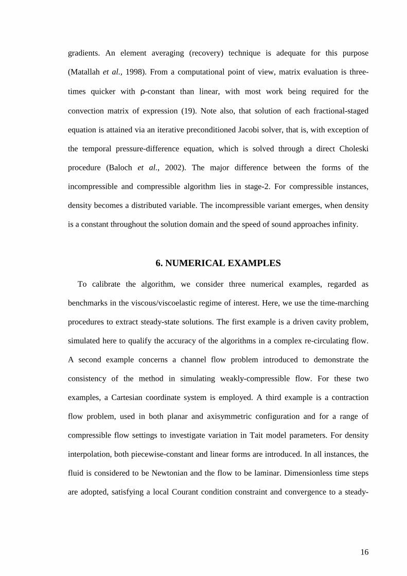
First, validation is sought for the incompressible algorithm, being conducted for
Re=100 and Re=400, as standard problem parameters. In Figure 1, contour patterns for
pressure and stream function are plotted based on case (b) with a regular mesh of 40*40
square sub-divisions, each split into two triangular elements. The contour results reflect
those shown in Zienkiewicz et al. (1995), Ghia et al. (1982), Peyret and Taylor (1983) and
Hawken et al. (1990). Pressure level lines illustrate, maxima (PA) is at the downstream lid-
corner and minima at the upstream corner (PB). The stream function contours display the
recirculating nature of the flow, with distortion near the singular corners, and a secondary
Moffatt-type vortex in the lower right-corner. Streamlines are twisted and distorted with
increase of convection (Re) towards the downstream corner, and the primary vortex centre

18
drops within the cavity. Stream function vortex centre values (S+) and (S*) are also
indicated. Figure 2 presents the computed incompressible velocity components along the
vertical and horizontal centerlines for Re=100 and Re=400. The results are contrasted
against those of Ghia et al. (1982), revealing close agreement and providing confidence in
the level of accuracy achieved for incompressible solutions. This position is also reflected
in solutions at Re=1, see Hawken et al. (1990).
For compressible flow under case (b) condition and Re=100, the two parameters
employed in the Tait state equation are fixed as (m,B)=(2,300), leading to Ma≈0.03 and
21% density increase above the incompressible state. In Figure 3, Mach number contours
are provided for piecewise-constant density interpolation (with recovery of the gradients).
The figure exhibits the singularity in the solution through the distortion in the Mach
number contours near the cavity top corners. In addition, pressure and streamline contour
patterns practically replicate those observed under the incompressible regime, and hence
are not reproduced for the compressible case.
Accuracy is assessed via the infinity norm, (∞hE ), on the longitudinal velocity, a
maximum norm of the difference from the fine mesh solution, scaled by the maximum of
all normed values. This is conducted, based on two types of density interpolation
(piecewise-constant with recovery of gradients and linear with constant gradients) under
Re=100. Both variable and constant lid-velocity profiles are investigated. Due to the lack
of an analytical solution, a fine mesh solution on 40x40 is taken as reference, against
which three further mesh solutions are compared (5x5, 10x10 and 20x20). Nodal values on
both cavity centerlines (X=0.5 and Y=0.5) are sampled for the computation of∞hE .
Figure 4a presents the pattern of behaviour in the infinite velocity error norm, with respect
to mesh-size reduction for case (a), variable lid-profile, and Re=100. Similar data are
reported for case (b), constant lid-profile, in Figure 4b. For the smooth solution (case a),

19
the order of accuracy for the three different implementations is above 2.5, approaching a
third-order. This order of accuracy has been achieved in some of our earlier work for
incompressible viscoelastic flows (Wapperom and Webster, 1998). For case (b), where the
solution presents singularities, the order is around 1.4. This is in keeping with expectation,
being well known that the presence of singularities in a problem will result in a decline in
accuracy (Hawken et al., 1990). Note, the same behaviour in error norm is detected in both
case (a) and (b), and for the three algorithmic implementations. This confirms that
modifications incorporated within the initial incompressible algorithm, to accommodate
weakly-compressible flows, do not degrade the accuracy of the pressure-correction method
itself.
Assessment of time-convergence to steady-state has been performed on case (b), based
on a 5x5 mesh and a time-step of ∆t=0.01, with initial conditions assigned as quiescent
(see Webster and Townsend (1990) for tracking of true transient solutions). Histories of the
relative error norms in velocity (Et(U)) and pressure (Et(P)) are provided in Figure 5 for
the three algorithmic variants. The results reflect a superior rate of convergence for the two
compressible algorithm forms, as compared to that for the incompressible algorithm: 30%
less time-steps are required for the compressible implementation to reach an equitable level
of tolerance (order of convergence is (O(2.6)) for compressible as compared to (O(2.4))
for incompressible forms). This we attribute to the improvement in system matrix
condition number, brought about via introduction of the mass-matrix, Mc and right-hand-
side adjustment viaρkL at stage 2 (see Eq.16). As a consequence, larger time-steps may be
selected within the compressible regime, as opposed to the incompressible alternative.
Note, the same rate of time-stepping convergence is observed in both compressible
algorithmic implementations.

20
6.2. Planar channel flow
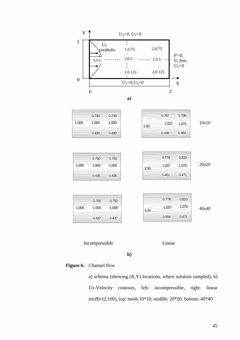
Specification for the channel flow problem is provided in Figure 6a. For viscous-
dominated liquid flows, this problem is a useful reference point. For incompressible flows,
an analytical solution is available, being devoid of complex geometric influence,
displaying one-dimensional shear-flow patterns. The compressible low Mach number
equivalent, provides quantitative reference data to be compared against its incompressible
counterpart. Here, inflow/outflow boundary conditions must be specified. The channel
dimensions are taken as two units long by one unit wide. No-slip boundary conditions are
assumed on solid boundaries. At flow-entry we consider a parabolic flow profile for the
longitudinal velocity UX, with maxima in UX imposed as unity. Cross-sectional component
UY vanishes at both entry and exit. At the outlet, the longitudinal velocity (UX) remains
unspecified (natural condition) and a reference pressure is fixed as zero. The Reynolds
number is considered as unity and compressibility Tait parameters (m,B), are assigned as
(2,100), to manifest influence of compressibility (Ma≈0.08 and 8% density elevated above
the incompressible state). Again, a time-step of t=0.01 is found suitable.
We begin by assessing the mass balance for this problem from inlet to outlet, via
satisfaction of the continuity equation. Results, based on three levels of regular mesh
refinement (rectangular sub-divisions split into triangles) and flow regime, are presented in
Table I. The error in the difference between flow entering and leaving the channel is
realised as O(0.1%) and less on the finer mesh, demonstrating conservation of mass
overall.
Velocity and Mach number field solutions in Figures 6 and 7 are presented with: top
figures for mesh 10*10, middle for 20*20 mesh and bottom 40*40 mesh. Quantification of
the different algorithmic variants (incompressible, compressible linear) are conveyed
through separate columns. Figure 6 presents the UX-velocity contours. To illustrate the

21
adjustment of velocity along the channel, solution values are in-laid at coordinate sample
locations are selected of (X=0.0, 1.0, 2.0), (Y=0.125, 0.50, 0.75), as depicted in Figure 6a.
UX-velocity contours are parallel to the flow in the incompressible regime, where the
velocity profile is parabolic. In either of the piecewise-constant or linear density
interpolation instances (only one shown), the flattening of velocity profile is more
pronounced and the smoothness of contours is improved by increasing mesh density. The
fact that velocity contours are not parallel reflects the convective nature of the flow. In
addition, for both piecewise-constant and linear interpolation representations
correspondence is close curved flow-speed compensates so as to satisfy mass conservation
at the outlet. This explains why, under equitable conditions, the outlet flow-speed is higher
in the compressible regime, as compared to that for incompressible flow.
Figure 7 presents corresponding Mach number contours (with in-laid solution values).
Note that, the speed of sound is infinite for an incompressible liquid, resulting in a
vanishing Mach number. Since density is related to pressure through the equation of state,
linked via the speed of sound, the Mach number reflects the relationship between velocity
and pressure. Thus, for piecewise-constant and linear density interpolation, the differences
observed in Mach number may be attributed to variation in pressure and velocity. In
addition, these results demonstrate the ability of the compressible implementations to deal
with low Mach number situations (Ma<8*10-2 ). Here, we observe yet again, a reasonable
correspondence between results for either density interpolation option (2% difference on
finest mesh).
Table II presents the values of the pressure and density along the centreline of the
channel at different X-locations (X=0.0,0.5,1.0,1.5,2.0) for the different implementations
and mesh size. Contours of pressure are level-lines across the flow cross-section. For
incompressible flow and with a mesh size 10*10, we recover the exact solution reflecting a

22
nondimensional inlet-outlet pressure-drop of 16 units. For compressible flow, with either
piecewise-constant or linear density interpolation, the pressure-drop is slightly elevated
over incompressible flow and increases with mesh-density (5% increase on the finest
mesh). In addition, with mesh size 40*40, we begin to detect departure in pressure profiles
contours from linear form (slightly parabolic). Note that for density, here results for the
incompressible liquid are suppressed, as density remains at a constant level.
Compressibility effects are apparent, with the density of the fluid entering the channel
being larger (by about 8% for both density representations) than that departing. As with
pressure, density contours degrade slightly from linear structure span-wise across the flow.
Since density at the inlet is larger, the flow-rate is greater in the compressible (piecewise-
constant or linear interpolation) as compared to the incompressible case. This explains the
reported corresponding elevation in pressure-drop of above.
6.3. Contraction flow
In the third benchmark, we introduce a more complex test problem typical of industrial
setting and with a view to viscoelastic computations to follow. This consists of a
contraction flow under both planar and axisymmetric reference, see Figure 8a. Here, we
observe larger pressure-drops than in straight channel flow above, and the effects of
compressibility are significant. The total length of the channel is taken as 76.5 units and the
contraction ratio is four to one. For this test problem, boundary conditions follow as
specified for the channel flow problem above, with a Reynolds number set to unity.
6.3.1. Planar contraction flow
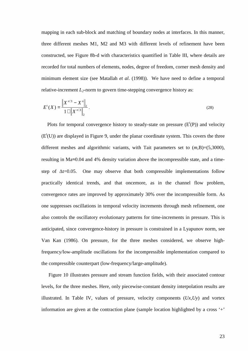
a) Mesh refinement: First, mesh refinement is conducted, based on a multi-block
meshing strategy to discretized the half-contraction channel-geometry, with conformal
23
mapping in each sub-block and matching of boundary nodes at interfaces. In this manner,
three different meshes M1, M2 and M3 with different levels of refinement have been
constructed, see Figure 8b-d with characteristics quantified in Table III, where details are
recorded for total numbers of elements, nodes, degree of freedom, corner mesh density and
minimum element size (see Matallah et al. (1998)). We have need to define a temporal
relative-increment L2-norm to govern time-stepping convergence history as:
2
12
1
1)(
+
+
+
−=
n
nn
t
X
XXXE . (28)
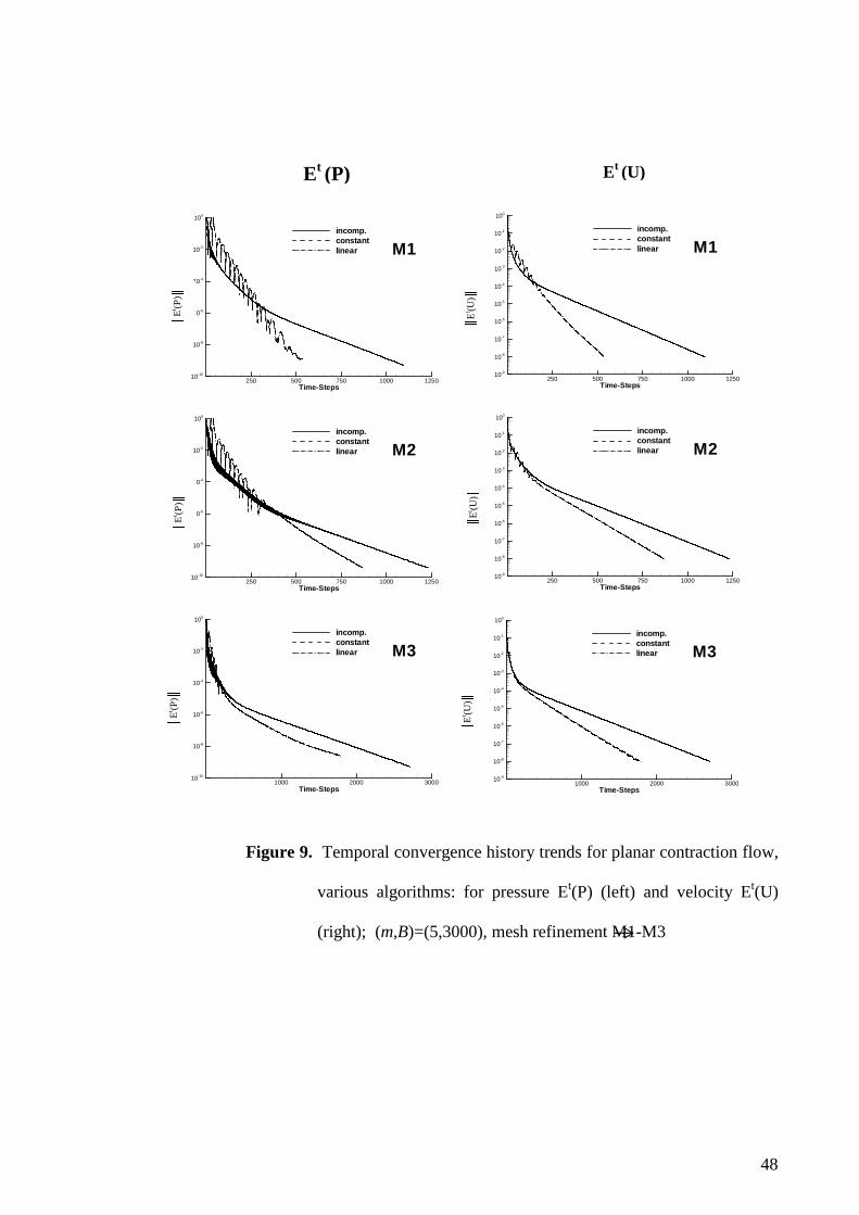
Plots for temporal convergence history to steady-state on pressure (Et(P)) and velocity
(Et(U)) are displayed in Figure 9, under the planar coordinate system. This covers the three
different meshes and algorithmic variants, with Tait parameters set to (m,B)=(5,3000),
resulting in Ma≈0.04 and 4% density variation above the incompressible state, and a time-
step of t=0.05. One may observe that both compressible implementations follow
practically identical trends, and that oncemore, as in the channel flow problem,
convergence rates are improved by approximately 30% over the incompressible form. As
one suppresses oscillations in temporal velocity increments through mesh refinement, one
also controls the oscillatory evolutionary patterns for time-increments in pressure. This is
anticipated, since convergence-history in pressure is constrained in a Lyapunov norm, see
Van Kan (1986). On pressure, for the three meshes considered, we observe high-
frequency/low-amplitude oscillations for the incompressible implementation compared to
the compressible counterpart (low-frequency/large-amplitude).
Figure 10 illustrates pressure and stream function fields, with their associated contour
levels, for the three meshes. Here, only piecewise-constant density interpolation results are
illustrated. In Table IV, values of pressure, velocity components (Ux,Uy) and vortex
information are given at the contraction plane (sample location highlighted by a cross ‘+’

24
in Figure 8a). Note, for the same compressibility setting, the piecewise-constant and the
linear density interpolations deliver identical results (differing by less than 0.025%) for a
particular mesh size (linear form suppressed). The associated contour plots are observed to
smooth with refinement. Note, that mesh M2 is felt adequate for detailed coverage below,
as this mesh is able to highlight the salient corner vortex and is computationally cost-
effective compared to the finest mesh M3.
b) Solutions at (m,B)=(2,300): Increasing compressible effects, via (m,B)=(2,300), leads
to Ma≈0.3. Here, there is variation in density above incompressible by about 65%,
exaggerated to highlight the difference between density representations. Figure 11, on
mesh M2, illustrates the adjustment across the density field for linear density interpolation,
and those in Mach number between piecewise-constant and linear density interpolations
around the contraction zone. Solutions point values for velocity, pressure, density and
Mach number are presented in tabular form (Table Va) at the sampled spatial locations
(a,b,c,d) of Figure 8d. In the pressure field, for instance, we observe about 1.5% difference
between both compressible representations. Generally, solution values at the sampled
locations are larger for compressible above incompressible flow (by about 25% in pressure
elevation). That is with the exception of X-velocity component (UX) at the location c,
where the flow slows down in the compressible case just prior to the contraction plane.
One notes that compressible conditions lead to conservation of mass-flow-rate in contrast
to volume-flow-rate for incompressible flows. In Mach number, contour field plots (Figure
11) reflect some differences (by about 9% at c-location), according to the choice of density
interpolation employed. This is because the Mach number is related to the speed of sound,
which itself is linked directly to density, via the Tait equation. Hence, the level of density

25
interpolation comes into play. One may observe, under piecewise-constant density
interpolation, Mach number contours are less-smooth over elements of larger size.
Figure 12 presents solution profiles for different variables (X-velocity, pressure, density
and Mach number) at the contraction channel centreline for both compressible
interpolation variants. The results provide clear evidence that low-order density
interpolation with gradient recovery, is able to reproduce results comparable to those with
linear density interpolation. Near the exit, a discrepancy of about 20%, at this level of
Mach number, is observed in Mach number, with those for constant density interpolation
being higher than those for the linear alternative. This departure is due mainly to the
adjustment in both velocity and pressure across the exit zone, and to some degree to the
mesh quality there.
6.3.2. Circular contraction flow
Under an axisymmetric frame of reference, pressure-differences exceed those for the
planar equivalent. Here, Tait parameters are set to (m,B)=(5,3000), leading to mild
compressible influences (Ma≈0.16, density elevated 17% above the incompressible state).
First, as above for planar flow, we confirm that similar trends are observed in field
variables based on both form of density interpolation (see Figures 13). Profiles over the
contraction channel centreline follow the planar case (as in Figure 12). Sampled solutions
values for the different variables are presented in Table Vb at the selected spatial locations
of Figure 8d. Oncemore, similar results are observed for both compressible representations
around this contraction zone (less than 0.1% in pressure). There is about 8% pressure
elevation in the compressible regime compared to the incompressible instance.

26
a) Tait parameter variation (m,B): We conduct a Tait parameter sensitivity analysis to
assess variation with the compressibility parameter set (m,B). First, we highlight the ability
of the compressible algorithm to deal with a range of low Mach number (0<Ma<0.2),
approaching the asymptotic limit Ma≈0. Figure 14 presents trends in solution profiles for
different variables at the contraction channel centreline, based on variation in
compressibility settings, adjusting Tait parameters accordingly. These trends reflect
adjustment from the incompressible towards the mildly compressible setting (Ma<0.2). In
the compressible regime, only piecewise-constant density interpolation has been employed,
as both constant and linear representations lead to practically identical results. Centreline
solution profiles indicate that the compressibility setting has little affect on the velocity
field before the contraction. As the flow becomes more compressible, some effects begin to
appear beyond the contraction zone, once the liquid accelerates (17% faster for
(m,B)=(5,3000)) above incompressible instance. At flow-entry, pressure and density are
larger for compressible above incompressible flow (8% for pressure and 17% for density
for (m,B)=(5,3000)). This highlights how much ‘compressibility’ impacts upon the flow
kinematics.
Second, in Figure 15, we provide compressible flow history numerical convergence
trends to steady-state for variation in (m,B) parameter set based upon increasing (Ma,ρ).
Experience shows that this is the important paring to extract corresponding convergence
behaviour in time. This covers 0.003<Ma<0.12 and 1.0001<ρ<1.13. All solutions are
pursued to a limiting tolerance of 10-8, though presentation in Figure 15 is restricted for
comparison purposes, to the first 1000 time-steps at a common time-step value of 5*10-2.
We comment that where convergence trends are replicated, across (m,B) setting providing
similar (Ma,ρ), say (m-variable,B=104) and (m=1,B-variable), practically identical field
solutions are obtained at steady-state.

27
At low Ma, Ma<0.005: high-frequency/low-amplitude oscillations are a characteristic in
the pressure norm Et(P) at early time (within the first 100 time-steps). The velocity norm
Et(U) remains smooth. The rate of convergence is higher in pressure (O( t3)) than in
velocity (O( t2.9)) up to around 250 time-steps, after which time both norms converge at
the same rate (that of velocity, with sustained gap between norms and monotonic linear
trends).
At moderate Ma (applicable for liquids), 0.01<Ma<0.08: there is elongation in pressure
norm oscillations, decreasing in frequency with increasing Ma. Trends are characterises by
lower frequency but larger amplitude pressure norm oscillations than for the low Ma-range.
Velocity norm oscillations begin to appear at and above Ma=0.03, spreading in time with
increasing Ma. The pressure norm oscillations remain in phase with and some three-times
larger than those in velocity, though clearly one drives the other. Equitable convergence
rates throughout time now begin to arise in both norms. Averaged rates are linear and
monotonic in pattern, being of order Et≈O( t2.1). Oscillatory Et(P) patterns in m=5 sub-
figures (e-g) are typical of convergence in a Lyapnov norm, as the theory would predict
(see Van Kan (1986)).
For Ma>0.1: oscillations in pressure and velocity norms disappear, so that convergence
trends are smooth, with monotonic linear convergence-patterns of equitable order,
Et≈O( t1.3). The marked difference here is the unification of convergence norm values
through time between the two variables of velocity and pressure. Clearly, the overall time
to achieve the limiting convergence tolerance of 10-8 will imply an increase in the number
of time-steps required. In the larger Ma≈0.12 instance, this leads to 1690 time-steps. This
adjusts to 865 for Ma≈0.04 and 750 for Ma≈0.005.
We conclude that such trends in numerical convergence behaviour may be harnessed to
gather the most preferable form for the instance in hand; speed in steady-state extraction or
28
matching both norms, Et(P) and Et(U). We note that it is the particular level of (Ma,ρ) that
dictates the numerical convergence response. Nevertheless, we may be able to take
advantage of superior convergence properties in adjusting (m,B) to arrive at a final steady-
state for the target pairing. We attribute the linearization of the Et(P) norms with increasing
Ma to the increased influence of the Mc-matrix in stage 2 (see Eq.(16)), an addition which
vanishes at steady-state. When only steady-state is sought, convergence behaviour could be
enhanced by choosing a large local time-step for stage 2. We note that by design, the
present approach is lacking to describe highly-compressible flow (Ma>>O(1)), as amongst
other things, this would necessitate consideration of a kinetic equation (which is neglected
here). Our experience is that numerical scaling on the pressure time-step at stage 2,
( tP=β t) may be a useful ploy that effectively switches the prevailing numerical value of
the speed of sound (c) in the denominator of Mc, thus capturing the temporal convergence
trend of an alternative physical (Ma,ρ)-pairing. To demonstrate this for t=0.05, we have
taken (Ma=0.12, ρ=1.13, β=1) and rescaled with β=10 to mimic (Ma=0.03, ρ=1.01, β=10),
for which we gather corresponding history norm convergence plots of Figures 15 (i) and
(e). This may be repeated with β=103 to mimic (Ma=0.003, ρ=1.0001, β=103) to recover
Figure 15 (a) convergence pattern. There is a strong resemblance here to pseudo-
compressible and artificial compressible implementations, employed for incompressible
flows, in the sense of stage 2 conditioning on the lhs of the equation.
b) Tending towards the incompressible limit (Ma→0): Here, we address the
effectiveness of the compressible implementation to deal with very low Mach number
situations (Ma≈0), via adjustment of the Tait parameter pairing (m, B), to mimic such a
state. To this end, in Figure 16, the Tait parameters are elevated to high levels (m=102 or
103 and B=105), and one observes improvement in stability and convergence-rate of the

29
compressible versus the incompressible implementations. At this level of Tait parameters
we observe high- frequency/low-amplitude pressure oscillations for incompressible
convergence trends that are practically suppressed in the compressible instance. This is
attributed to improvement in system condition number, via inclusion of the stage 2 mass-
matrix and right-hand-side terms. Sample solution values for this particular case are
tabulated in Table VI. The data highlight the match in sample centreline solution values,
between incompressible and compressible (with Ma≈0) algorithmic implementations, in all
variables and over different regions. Results demonstrate that, in the zero Mach number
limiting regime, piecewise-constant density interpolation, with recovery of gradients
during the second stage, is equitable to linear density interpolation. On the other hand,
there is less than 0.5% overall difference between incompressible and compressible
representations. Based on these findings, we have established that the compressible
algorithmic implementations may be employed effectively to simulate weakly-
compressible, as well as incompressible flow scenarios.
7. CONCLUSIONS
Based on a second order FE approximation with a pressure-correction method split into
three distinguish fractional stages, two algorithmic representations have been introduced to
simulate weakly-compressible highly-viscous polymeric liquid flow. The first uses a
piecewise-constant density interpolation on the finite element, with nodal-recovery to
compute the gradient of density. The second variant is based on a linear interpolation for
the density (hence, piecewise-constant density gradient).
Consistency, accuracy and convergence have been assessed on a series of benchmark
problems to highlight the performance of both interpolation variants. There is no apparent
loss of accuracy incurred through these compressible interpolation variants, as compared to

30
their incompressible counterpart on these test problems. This is anticipated to reach a third-
order for continuous problems. The convergence-rate to steady-state of both interpolation-
forms is improved upon, as compared to that of the incompressible flow algorithm. This is
attributed to the improvement in system condition number via the mass-matrix and right-
hand-side contribution to the second-stage equation (for pressure). We have established
temporal convergence patterns for compressible implementations conveying alternative
ranges of (Ma,ρ). Also, we have been able to point to scaling adjustment to improve
convergence behaviour to steady-state solutions.
These compressible algorithmic variants have been shown capable of simulating flow
with low to zero Mach number. Hence, a zero Mach number limit may be reached by
adjusting Tait parameter pairings, where compressibility effects within the liquid flow may
be controlled whilst approaching the incompressible limit. Under such circumstances,
results match well with those for the compressible algorithm and those for the ‘purely’
incompressible algorithm. These findings allow the user to apply the compressible
algorithm for both compressible and incompressible regimes.
The programming effort required to implement these compressible algorithms within an
incompressible software framework has been manageable. The implementation is
considerably easier for the piecewise-constant density interpolation (incompressible at the
element-level, see Hawken et al., 1990, for operation count analysis indicating linear time
complexity on node (or element) counts per time-step, and linear space complexity
overall). This necessitates a recovery technique for density gradients at stage two, with
density scaling of all elemental matrices. In addition, low-order density interpolation with
gradient recovery, has been found to perform equally as well as a linear density
interpolation. On these grounds, the piecewise-constant interpolation is strongly

31
commended. Next, attention will be devoted to analysing viscoelastic counterpart flows,
seeking to investigate the numerical and physical impact of this methodology there also.
ACKNOWLEDGMENTS
The financial support of EPSRC grant GR/R46885/01 is gratefully acknowledged. The
second author welcomes the financial support of the Islamic Republic of Iran.

32
REFERENCES
Baaijens, P. T. F. (1998) "Mixed finite element methods for viscoelastic flow analysis: a
review", Journal of Non-Newtonian Fluid Mechanics, Vol 79, No 2-3, pp. 361-385.
Baloch, A., Grant, P. W. and Webster, M. F. (2002) "Parallel computation of two-
dimensional rotational flows of viscoelastic fluids in cylindrical vessels",
Engineering Computations, Vol 19, No 7, pp. 820 - 853.
Bijl, H. and Wesseling, P. (1998) "A unified method for computing incompressible and
compressible flows in boundary-fitted coordinates", Journal of Computational
Physics, Vol 141, No 2, pp. 153-173.
Brujan, E. A. (1999) "A first-order model for bubble dynamics in a compressible
viscoelastic liquid", Journal of Non-Newtonian Fluid Mechanics, Vol 84, No 1, pp.
83-103.
Chorin, A. J. (1968) "Numerical solution of the Navier-Stokes equations", Mathematics of
Computation, Vol 22, pp. 745-762.
Ding, D., Townsend, P. and Webster, M. F. (1995) "On computation of two and three-
dimensional unsteady thermal non-Newtonian flows", International Journal of
Numerical Methods in Heat and Fluid Flow, Vol 5, No 6, pp. 495-510.
Donea, J., Giuliani, S., Laval, H. and Quartapelle, L. (1982) "Finite element solution of the
unsteady Navier-Stokes equations by fractional step method", Computer Methods
in Applied Mechanics and Engineering, Vol 30, pp. 53-73.
Field, J. E. (1999) "ELSI conference: invited lecture: Liquid impact: theory, experiment,
applications", Wear, Vol 233-235, pp. 1-12.
Georgiou, G. C. (2003) "The time-dependent, compressible Poiseuille and extrudate-swell
flows of a Carreau fluid with slip at the wall", Journal of Non-Newtonian Fluid
Mechanics, Vol 109, No 2-3, pp. 93-114.

33
Ghia, U., Ghia, K. N. and Shin, C. (1982) "High-Re solutions for incompressible flow
using the Navier-Stokes equations and a multigrid method", Journal of
Computational Physics, Vol 48, pp. 387-411.
Guénette, R. and Fortin, M. (1995) "A new mixed finite element method for computing
viscoelastic flows", Journal of Non-Newtonian Fluid Mechanics, Vol 60, No 1, pp.
27-52.
Guillard, H. and Viozat, C. (1999) "On the behaviour of upwind schemes in the low Mach
number limit", Computers & Fluids, Vol 28, No 1, pp. 63-86.
Han, K.-H. and Im, Y.-T. (1997) "Compressible flow analysis of filling and post-filling in
injection molding with phase-change effect", Composite Structures, Vol 38, No 1-
4, pp. 179-190.
Harlow, F. H. and Amsden, A. (1968) "Numerical calculation of almost incompressible
flow", Journal of Computational Physics, Vol 3, pp. 80-93.
Hawken, D. M., Tamaddon-Jahromi, H. R., Townsend, P. and Webster, M. F. (1990) "A
Taylor-Galerkin based algorithm for viscous incompressible flow", International
Journal for Numerical Methods in Fluids, Vol 10, pp. 327-351.
Huang, Y. K. and Chow, C. Y. (1974) "The generalized compressibility equation of Tait
for dense matter", Journal of Physics D: Applied Physics, Vol 7, pp. 2021-2023.
Hughes, T. J. R., Franca, L. P. and Hulbert , G. M. (1989) "A new finite element
formulation for computational fluid dynamics: VIII. The Galerkin Least-Squares
method for advective diffusive equations", Computer Methods in Applied
Mechanics and Engineering, Vol 73, p 173–189.
Jackson, M. J. and Field, J. E. (1999) "Liquid impact erosion of single-crystal magnesium
oxide", Wear, Vol 233-235, pp. 39-50.

34
Jenny, P. and Muller, B. (1999) "Convergence acceleration for computing steady-state
compressible flow at low Mach numbers", Computers & Fluids, Vol 28, No 8, pp.
951-972.
Karimian, S. M. H. and Schneider, G. E. (1995) "Pressure-based control-volume finite-
element method for flow at all speeds", AIAA journal, Vol 33, No 9, pp. 1611-
1618.
Karki, K. and Patankar, S. V. (1989) "Pressure based calculation procedure for viscous
flows at all speeds in arbitrary configurations", AIAA journal, Vol 27, No 9, pp.
1167-1174.
Kelmanson, M. A. and Maunder, S. B. (1999) "Modelling high-velocity impact phenomena
using unstructured dynamically-adaptive Eulerian meshes", Journal of the
Mechanics and Physics of Solids, Vol 47, No 4, pp. 731-762.
Keshtiban , I. J., Belblidia, F. and Webster, M. F.,(2003) "Review of compressible flow
solvers for low Mach number flows: density-based approach," Computer Science
Technical Report., University of Wales Swansea, UK.
Lien, F. S. and Leschziner, M. A. (1993) "A pressure velocity solution strategy for
compressible flow and its application to shock boundary layer interaction using
second-moment turbulance closure", Journal of Fluid Engineering, Vol 115, No
DEC, pp. 717-725.
Löhner, R., Morgan, K. and Zienkiewicz, O. C. (1984) "The solution of non-linear
hyperbolic equation systems by the finite element method", International Journal
for Numerical Methods in Fluids, Vol 4, pp. 1043-1063.
Mary, I., Sagaut, P. and Deville, M. (2000) "An algorithm for low Mach number unsteady
flows", Computers & Fluids, Vol 29, No 2, pp. 119-147.

35
Matallah, H., Townsend, P. and Webster, M. F. (1998) "Recovery and stress-splitting
schemes for viscoelastic flows", Journal of Non-Newtonian Fluid Mechanics, Vol
75, No 2-3, pp. 139-166.
Moukalled, F. and Darwish, M. (2001) "A high-resolution pressure-based algorithm for
fluid Flow at all speeds", Journal of Computational Physics, Vol 168, No 1, pp.
101-133.
Munz, C.-D., Roller, S., Klein, R. and Geratz, K. J. (2003) "The extension of
incompressible flow solvers to the weakly compressible regime", Computers &
Fluids, Vol 32, No 2, pp. 173-196.
Ngamaramvaranggul, V. and Webster, M. F. (2000a) "Computation of free surface flows
with a Taylor-Galerkin/pressure-correction algorithm", International Journal for
Numerical Methods in Fluids, Vol 33, No 7, pp. 993-1026.
Ngamaramvaranggul, V. and Webster, M. F. (2000b) "Simulation of coating flows with
slip effects", International Journal for Numerical Methods in Fluids, Vol 33, No 7,
pp. 961-992.
Patankar, S. V. (1980) Numerical heat transfer and fluid flow, McGraw-Hill, New York.
Peyret, R. and Taylor, T. D. (1983) Computational Methods for Fluid Flow, Springer-
Verlag, New York.
Ranganathan, M., Mackley, M. R. and Spitteler, P. H. J. (1999) "The application of the
multipass Rheometer to time dependent capillary flow measurements of a
Polyethylene melt", Journal of Rheology, Vol 43, No 2, pp. 443-451.
Roller, S. and Munz, C. D. (2000) "A low Mach number scheme based on multi-scale
asymptotics", Computing and Visualization in Science, Vol 3, No 1/2, pp. 85-91.
36
Saramito, P. and Piau, J. M. (1994) "Flow characteristics of viscoelastic fluids in an abrupt
contraction by using numerical modeling", Journal of Non-Newtonian Fluid
Mechanics, Vol 52, No 2, p 263.
Tait, P. G. (1888) "HSMO", London, Vol 2, No 4.
Temam, R. (1969) "Sur l'approximation de la solution de Navier-Stokes par la méthode des
pas fractionnaires", Archiv. Ration. Mech. Anal., Vol 32, pp. 377-385.
Turkel, E., Radespiel, R. and Kroll, N. (1997) "Assessment of preconditioning methods for
multidimensional aerodynamics", Computers & Fluids, Vol 26, No 6, pp. 613-634.
Van Kan, J. (1986) "A second-order accurate pressure-correction scheme for viscous
incompressible flow", SIAM Journal of Scientific and Statistical Computing, Vol 7,
pp. 870-891.
Walters, K. and Webster, M. F. (2003) "The distinctive CFD challenges of computational
rheology", International Journal for Numerical Methods in Fluids, Vol In press.
Wapperom, P. and Webster, M. F. (1998) "A second-order hybrid finite-element/volume
method for viscoelastic flows", Journal of Non-Newtonian Fluid Mechanics, Vol
79, No 2-3, pp. 405-431.
Webster, M. F. and Townsend, P. (1990) In Numerical Methods in Engineering: Theory
and Applications - NUMETA, Vol. 90 (Eds, Pande, G. N. and Middleton, J.)
Elsevier
Applied Science, London & New York.
Wong, J. S., Darmofal, D. L. and Peraire, J. (2001) "The solution of the compressible Euler
equations at low Mach numbers using a stabilized finite element algorithm",
Computer Methods in Applied Mechanics and Engineering, Vol 190, No 43-44, pp.
5719-5737.
37
Wu, Y.-S. and Pruess, K. (2000) "Integral solutions for transient fluid flow through a
porous medium with pressure-dependent permeability", International Journal of
Rock Mechanics and Mining Sciences, Vol 37, No 1-2, pp. 51-61.
Zienkiewicz, O. C., Morgan, K., Sataya Sal, B. V. K., Codina, R. and Vasquez, M. (1995)
"A general algorithm for compressible and incompressible flow - Part II . Test on
the explicit form", International Journal for Numerical Methods in Fluids, Vol 20,
pp. 887-913.

38
List of figures
Figure 1. Pressure (top) and streamlines (bottom) contours for cavity: Incompressible,
case (b), Re=100 (left) and Re=400 (right)
Figure 2. U,V) on vertical or horizontal cavity centrelines, incompressible, case (b), Re=
100 and Re= 400
Figure 3. Mach number contours for cavity: Piecewise-constant density interpolation,
case (b), Re=100, (m,B)=(2,300)
Figure 4. Infinity error norm ∞hE on velocity for different algorithms for cavity, a)
case (a), Re=100, b) case (b), Re=100, (m,B)=(2,300)
Figure 5. Temporal convergence history trends for velocity, Et(U) (left) and pressure,
Et(P) (right): Cavity problem based on Re=100 and ∆t=0.01, case (b),
(m,B)=(2,300)
Figure 6. Channel flow, a) schema (showing (X,Y) locations, where solution sampled),
b) Ux-Velocity contours, left: incompressible, right: linear (m,B)=(2,100), top:
mesh 10*10, middle: 20*20, bottom: 40*40
Figure 7. Ma*102 contours for channel, left: piecewise-constant, right: linear, top: mesh
10*10, middle: 20*20, bottom: 40*40, (m,B)=(2,100)
Figure 8. Contraction flow. a) schema, b-d) Mesh refinement around the contraction,
M1-M3), d) Sample point locations on mesh M2 for axisymmetric and planar
cases. (mesh characteristics in Table III)
Figure 9. Temporal convergence history trends for planar contraction flow, various
algorithms: for pressure Et(P) (left) and velocity Et(U) (right); (m,B)=(5,3000),
mesh refinement M1-M3

39
Figure 10. Pressure (right) and streamlines fields (left) for planar contraction flow
problem, piecewise-constant density interpolation scheme, (m,B)=(5,3000),
mesh refinement M1-M3 (values in Table IV)
Figure 11. Density and Mach number for planar contraction flow, (m,B)=(2,300); a)
Density (linear interpolation), Mach number under b) piecewise density
interpolation c) linear density interpolation (values in Table Va)
Figure 12. Solution profiles at channel centreline (planar case), piecewise-constant and
linear density interpolation, (m,B)=(2,300). Top left: velocity, top right:
pressure, bottom left: density, bottom right: Mach number
Figure 13. Density and Mach number for circular contraction flow, (m,B)=(5,3000); a)
Density (linear interpolation), Mach number under b) piecewise density
interpolation c) linear density interpolation (values in Table Vb)
Figure 14. Variation in compressibility settings, mildly compressible towards
incompressible, trends in solution profiles on channel centreline (circular case),
piecewise-constant density interpolation. top left: UZ-velocity, top right:
pressure, bottom left: density, bottom right: Mach number
Figure 15. Effect of Tait parameter (m,B) variation on convergence history of pressure
Et(P) and velocity Et(U), piecewise-constant density interpolation, increasing
compressibility effect, circular contraction flow
Figure 16. Convergence history trends for (left) velocity Et(U) and (right) pressure Et(P),
circular contraction flow, incompressible versus piecewise-constant density
interpolation tending to the incompressible limit

40
Figure 1. Pressure (top) and streamlines (bottom) contours for cavity:
Incompressible, case (b), Re=100 (left) and Re=400 (right)
Re=10 Re=40
12
2
4
4
5
5
6
6
7
7
7
8
8
910
3
3 Level P10 220.09 210.08 200.07 199.76 199.45 197.04 195.03 193.02 192.01 190.0
PA=463.1
A
2
1
3
4
5
6
7
8
Level S10 7.6x10-06
9 1.2x10-06
8 -1.0x10-04
7 -2.0x10-03
6 -1.0x10-02
5 -3.0x10-02
4 -5.0x10-02
3 -7.0x10-02
2 -9.0x10-02
1 -1.0x10-01
S+=-0.101
S*=9.87x10⁻⁶
+
*
1
2
3
4
38
87
9106
567
8
3
5
4
Level P10 300.09 200.08 162.07 161.56 160.05 158.04 153.43 150.02 135.51 125.6
PA=610.7
A
12
34
5
6
710
9
Level S10 2.0x10-04
9 1.9x10-05
8 1.0x10-07
7 -1.0x10-04
6 -1.0x10-02
5 -3.0x10-02
4 -5.0x10-02
3 -7.0x10-02
2 -9.0x10-02
1 -1.0x10-01
S+=-0.107
S*=+0.472x10⁻³
400
+
*
A A B B
PA=463.1 PA=610.7
S+=-0.101 S*=9.87x10⁻⁶
S+=-0.107 S*=0.472x10⁻³

41
Figure 2. (U,V) on vertical or horizontal cavity centrelines, incompressible,
case (b), Re= 100 and Re= 400
Velocity
Ver
tical
/Hor
izon
talD
ista
nce
-0.25 0 0.25 0.5 0.75 10
0.1
0.2
0.3
0.4
0.5
0.6
0.7
0.8
0.9
1
Present results ( u component )Ghia et al. ( u component )Present results ( v component )Ghia et al. ( v component )
Re = 100
Velocity
Ver
tical
/Ho
rizo
ntal
Dis
tanc
e
-0.5 -0.25 0 0.25 0.5 0.75 10
0.1
0.2
0.3
0.4
0.5
0.6
0.7
0.8
0.9
1
Present results ( u component )
Ghia et al. ( u component )
Present results ( v component )
Ghia et al. ( v component )
Re=400

42
Figure 3. Mach number contours for cavity: Piecewise-constant density
interpolation, case (b), Re=100, (m,B)=(2,300)
1
11
1
2
3
3
4
45
5
6
6
7
7
2
8
X
Y
0 0.5 1
0.1
0.2
0.3
0.4
0.5
0.6
0.7
0.8
0.9
1
Level MACH8 0.02507 0.01506 0.01205 0.00904 0.00753 0.00502 0.00151 0.0001
Level Ma

43
a) b)
Figure 4. Infinity error norm ∞hE on velocity for different algorithms for
cavity, a) case (a), Re=100, b) case (b), Re=100, (m,B)=(2,300)
h
||E
h(U
)||
0.1 0.2 0.3 0.4 0.5
10-3
10-2
10-1
linear (h 2.59)
piece-wise (h 2.56)
incomp. (h 2.71)
case (a)
∞
linear (h2.59) constant (h2.56) incomp. (h2.71)
h
||E
h(U
)||
0.1 0.2 0.3 0.4 0.5
0.02
0.04
0.06
0.08
0.1
linear (h 1.55)
piece-wise (h 1.38)
incomp. (h 1.53)
case (b)
∞
linear (h1.55) constant (h1.38) incomp. (h1.53)
case (a) case (b)

44
Figure 5. Temporal convergence history trends for velocity, Et(U) (left) and
pressure, Et(P) (right): Cavity problem based on Re=100 and
∆t=0.01, case (b), (m,B)=(2,300)
Time-Steps
Et(U
)
100 200 300 40010-9
10-8
10-7
10-6
10-5
10-4
10-3
10-2
10-1
100
incomp.
constant
linear
Time-Steps
Et(p
)
100 200 300 40010-8
10-7
10-6
10-5
10-4
10-3
10-2
10-1
100
incomp.
constant
linear Et (P
)
Et (U
)
45
a)
Incompressible Linear
b)
Figure 6. Channel flow
a) schema (showing (X,Y) locations, where solution sampled), b)
Ux-Velocity contours, left: incompressible, right: linear
(m,B)=(2,100), top: mesh 10*10, middle: 20*20, bottom: 40*40
P=0, Ux free, UY=0
UX=0, UY=0
UX=0,UY=0
2
1
Y
X
0
0
UX parabolic
1,0.5
1,0.75
1,0.125
2,0.751
2,0.5
2,0.125
0,0.5
1.000 1.000
0.430
0.740 0.740
0.430
1.000
1.000 1.000
0.435
0.750 0.750
0.435
1.000
1.000 1.000
0.437
0.750 0.750
0.437
1.000
10x10
20x20
40x40
1.001.037
0.451
0.778 0.810
0.471
1.075
1.001.037
0.446
0.767 0.796
0.464
1.075
1.001.037
0.454
0.778 0.810
0.471
1.076

46
Piecewise-constant Linear
Figure 7. Ma*102 contours for channel, left: piecewise-constant, right: linear,
top: mesh 10*10, middle: 20*20, bottom: 40*40, (m,B)=(2,100)
10x10
20x20
40x40
6.785 7.163
3.082
5.302 5.610
3.270
7.5806.772 7.186
3.091
5.336 5.701
3.317
7.694
6.783 7.221
3.162
5.417 5.817
3.399
7.748
6.779 7.211
3.139
5.413 5.808
3.372
7.729 6.785 7.162
3.117
5.373 5.701
3.321
7.579
6.785 7.162
3.135
5.373 5.707
3.348
7.584

47
Figure 8. Contraction flow.
a) schema, b-d) Mesh refinement around the contraction, M1-M3),
d) Sample point locations on mesh M2 for axisymmetric and planar
cases. (mesh characteristics in Table III)
c)
7.5 27.5
76.5
1
UX=0, UY=0
UY=0
P=0, UX free, UY=0
4
Y X
+ a) b) d)
M1 M3
14 16 18 20 22 240
1
2
3
4
+b+a
+d+c
Z
R M2
M3 M1
48
Figure 9. Temporal convergence history trends for planar contraction flow,
various algorithms: for pressure Et(P) (left) and velocity Et(U)
(right); (m,B)=(5,3000), mesh refinement M1-M3
Et (P) Et (U)
Time-Steps
Et(p
)
1000 2000 300010-10
10-8
10-6
10-4
10-2
100
incomp.constantlinear M3
Time-Steps
Et(p
)
250 500 750 1000 125010-10
10-8
10-6
10-4
10-2
100
incomp.constantlinear M2
Time-Steps
Et(p
)
250 500 750 1000 125010-10
10-8
10-6
10-4
10-2
100
incomp.constantlinear M1
Time-Steps
Et(U
)
250 500 750 1000 125010-9
10-8
10-7
10-6
10-5
10-4
10-3
10-2
10-1
100
incomp.constantlinear M1
Time-Steps
Et(U
)
250 500 750 1000 125010-9
10-8
10-7
10-6
10-5
10-4
10-3
10-2
10-1
100
incomp.constantlinear M2
Time-Steps
Et(U
)
1000 2000 300010-9
10-8
10-7
10-6
10-5
10-4
10-3
10-2
10-1
100
incomp.constantlinear M3
Et (P
)
Et (P
)
Et (P
)
Et (U
)
Et (U
)
Et (U
)

49
Figure 10. Pressure (right) and streamlines fields (left) for planar contraction
flow, piecewise-constant density interpolation scheme,
(m,B)=(5,3000), mesh refinement M1-M3 (values in Table IV)
Density ( -linear interpolation)
Mach number (-constant interpolation)
Mach number (-linear interpolation)
1
3
57
Level MACH8 0.1357 0.1206 0.0455 0.0324 0.0283 0.0212 0.0091 0.001
1
5
56
6
3
8
Level DEN8 1.64157 1.64136 1.64125 1.64114 1.64043 1.62502 1.60001 1.5700
1
1
3
5 7
Level MACH8 0.1337 0.1206 0.0455 0.0324 0.0283 0.0212 0.0091 0.001
a) b) c)

50
Figure 11. Density and Mach number for planar contraction flow, (m,B)=(2,300); a)
Density (linear interpolation), Mach number under b) piecewise density
interpolation c) linear density interpolation (values in Table Va)
Pressure Stream function
1234
5
56
67
7
Level P7 410.966 410.845 410.744 410.383 408.972 396.481 388.75
M1
123
4
5
56
67
7
Level P7 410.936 410.835 410.734 410.323 408.982 396.091 387.05
M2
1234
5
5
66
7
7
Level P7 410.936 410.835 410.734 410.323 408.982 396.091 387.05
M3
3
4
5
6Level S6 1.6x10+00
5 7.0x10-01
4 1.8x10-01
3 4.0x10-03
2 -1.0x10-04
1 -2.0x10-042
3
4
5
6Level S6 1.8x10+00
5 8.5x10-01
4 2.5x10-01
3 4.0x10-03
2 -1.0x10-04
1 -2.0x10-04
3
4
5
6Level S6 1.6x10+00
5 7.0x10-01
4 1.8x10-01
3 4.0x10-03
2 -1.0x10-04
1 -2.0x10-04
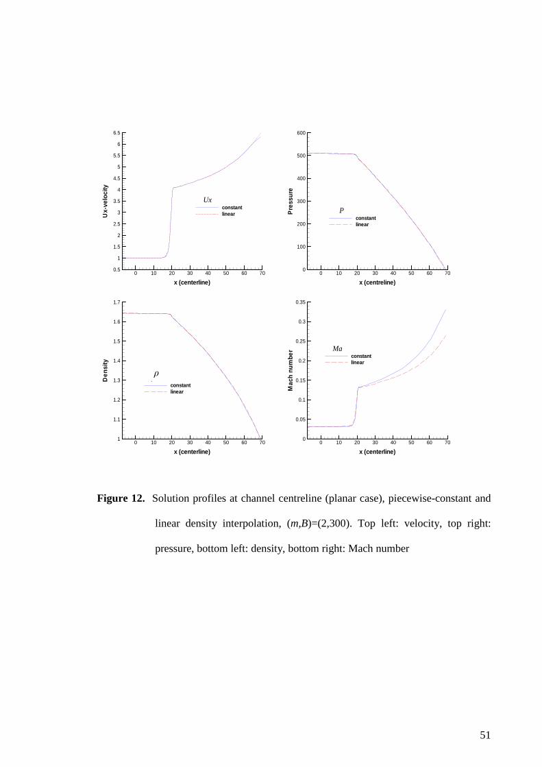
51
Figure 12. Solution profiles at channel centreline (planar case), piecewise-constant and
linear density interpolation, (m,B)=(2,300). Top left: velocity, top right:
pressure, bottom left: density, bottom right: Mach number
x (centerline)
Mac
hnu
mbe
r
0 10 20 30 40 50 60 700
0.05
0.1
0.15
0.2
0.25
0.3
0.35
constantlinear
Ma
x (centerline)
Den
sity
0 10 20 30 40 50 60 701
1.1
1.2
1.3
1.4
1.5
1.6
1.7
constantlinear
ρ
x (centerline)
Ux-
velo
city
0 10 20 30 40 50 60 700.5
1
1.5
2
2.5
3
3.5
4
4.5
5
5.5
6
6.5
constantlinear
Ux
x (centreline)P
ress
ure
0 10 20 30 40 50 60 700
100
200
300
400
500
600
constantlinear
P
ρ
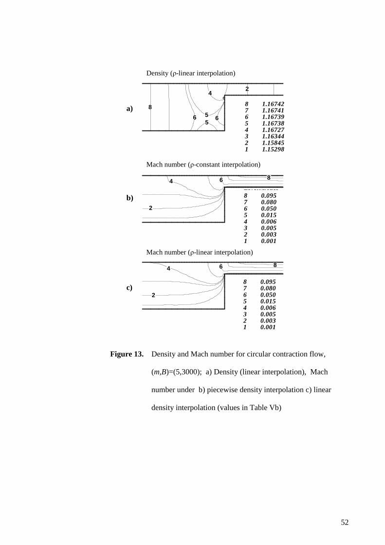
52
Figure 13. Density and Mach number for circular contraction flow,
(m,B)=(5,3000); a) Density (linear interpolation), Mach
number under b) piecewise density interpolation c) linear
density interpolation (values in Table Vb)
2
4 6 8
LevelMACH8 0.0957 0.0806 0.0505 0.0154 0.0063 0.0052 0.0031 0.001
Density ( -linear interpolation)
4
5
2
56 6
8
Level DEN8 1.167427 1.167416 1.167395 1.167384 1.167273 1.163442 1.158451 1.15298
8
2
4 6LevelMACH8 0.0957 0.0806 0.0505 0.0154 0.0063 0.0052 0.0031 0.001
Mach number (-constant interpolation)
a) b) c)
Mach number (-linear interpolation)

53
Figure 14. Variation in compressibility settings, mildly compressible towards
incompressible, trends in solution profiles on channel centreline (circular
case), piecewise-constant density interpolation. top left: UZ-velocity, top
right: pressure, bottom left: density, bottom right: Mach number
Z (Centerline)
Den
sity
0 10 20 30 40 50 60 70
1
1.05
1.1
1.15
1.2B=3x10⁴ m=10B=3x10³ m=10B=3x10³ m=5
Z (Centerline)
UZ
-vel
ocity
0 10 20 30 40 50 60 700
2
4
6
8
10
12
14
16
18
20
Incomp.B=3x10⁴ m=10B=3x10³ m=10B=3x10³ m=5
UZ
Z (Centerline)
Pre
ssur
e
0 10 20 30 40 50 60 700
500
1000
1500
2000
2500
3000
3500
Incomp.B=3x10⁴ m=10B=3x10³ m=10B=3x10³ m=5
P
Z (Centerline)
Mac
hnu
mbe
r
0 10 20 30 40 50 60 70
0
0.02
0.04
0.06
0.08
0.1
0.12
0.14
0.16
0.18
B=3x10⁴ m=10B=3x10³ m=10B=3x10³ m=5
Ma
ρ
P
UZ
Ma

54
Figure 15. Effect of Tait parameter (m,B) variation on convergence history of
pressure Et(P) and velocity Et(U), piecewise-constant density
interpolation, increasing compressibility effect, circular contraction flow
Time-Steps
Et (P
),E
t (U)
0 250 500 750 100010-10
10-8
10-6
10-4
10-2
100
PressureVelocity
B=104, m=2.5*10 - B=3*105, m=1.0
Ma= 0.03ρ= 1.01
Time-Steps
Et (P
),E
t (U)
0 250 500 750 100010-10
10-8
10-6
10-4
10-2
100
PressureVelocity
B=3*104, m=5
Ma= 0.04ρ= 1.02
Time-Steps
Time-Steps
Et (P
),E
t (U)
0 250 500 750 100010-10
10-8
10-6
10-4
10-2
100
PressureVelocity
B=104, m=2.5*102 - B=3*106, m=1.0
Ma= 0.010ρ= 1.001
d) e) f)
Time-Steps
Et (P
),E
t (U)
0 250 500 750 100010-10
10-8
10-6
10-4
10-2
100
PressureVelocity
B=104, m=10 - B=105, m=1.0
Ma= 0.05ρ= 1.03
Time-Steps
Et (P
),E
t (U)
0 250 500 750 100010-10
10-8
10-6
10-4
10-2
100
PressureVelocity
B=104, m=2.5 - B=3*104, m=1.0
Ma= 0.12ρ= 1.13
Time-Steps
Et (P
),E
t (U)
0 250 500 750 100010-10
10-8
10-6
10-4
10-2
100
PressureVelocity
B=104, m=5
Ma= 0.08ρ= 1.06
g) h) i)
Time-Steps
Et (P
),E
t (U)
0 250 500 750 100010-10
10-8
10-6
10-4
10-2
100
PressureVelocity
B=104, m=2.5*103 - B=3*107, m=1.0
Ma= 0.003ρ= 1.0001
Time-Steps
Et (P
),E
t (U)
0 250 500 750 100010-10
10-8
10-6
10-4
10-2
100
PressureVelocity
B=104, m=103 - B=107, m=1.0
Ma= 0.005ρ= 1.0003
Time-Steps
Et (P
),E
t (U)
0 250 500 750 100010-10
10-8
10-6
10-4
10-2
100
PressureVelocity
B=3*106, m=5
Ma= 0.004ρ= 1.0002
a) b) c)

55
Figure 16. Convergence history trends for (left) velocity Et(U) and (right) pressure
Et(p), circular contraction flow problem, incompressible versus
piecewise-constant density interpolation tending to the incompressible
limit
Time-Steps
Et(U
)
100 200 300 400 500 600 700 800 900
10-8
10-7
10-6
10-5
10-4
10-3
10-2
10-1
100
Incomp.B=105, m=103
B=105, m=102
Piece-wiese constant
Time-Steps
Et(p
)
100 200 300 400 500 600 700 800 900
10-9
10-8
10-7
10-6
10-5
10-4
10-3
10-2
10-1
100
Incomp.B=105, m=103
B=105, m=102
Piece-wiese constant
Et(U) Et(P)
56
List of tables
Table I. Error on mass balance for channel flow under different regimes and meshes,
(m,B)=(2,100)
Table II. Pressure and density values for channel flow under three regimes, centreline
various X-locations with mesh-size variation, (m,B)=(2,100)
Table III. Mesh characteristic parameters for contraction flow
Table IV. Sample pressure and velocity components values at contraction and vortex
information, various meshes and different algorithms, planar contraction flow,
(m,B)=(5,3000)
Table V. Solution values at sampled spatial locations of contraction flow, various
algorithms, a) planar case, (m,B)=(2,300), b) circular case, (m,B)=(5,3000)
Table VI. Sampled centreline solution values, various algorithms, towards zero Mach
number (circular case)

57
Table I. Error on mass balance for channel flow under different regimes and meshes,
(m,B)=(2,100)
Incompressible Piecewise-constant Linear
Mesh Inlet Outlet %Error Inlet Outlet %Error Inlet Outlet %Error
10*10 0.6667 0.6650 0.250 0.7148 0.7088 0.832 0.7148 0.7130 0.259
20*20 0.6667 0.6625 0.063 0.7160 0.7131 0.407 0.7162 0.7152 0.137
40*40 0.6667 0.6666 0.016 0.7164 0.7149 0.209 0.7165 0.7160 0.076

58
Table II. Pressure and density values for channel flow under three regimes, centreline
various X-locations with mesh-size variation, (m,B)=(2,100)
X- positions
Mesh 10*10
Mesh 20*20
Mesh 40*40
0.0 16.000 16.000 16.000 0.5 12.000 12.000 12.000 1.0 8.000 8.000 8.000
Incomp-ressible 1.5 4.000 4.000 4.000
0.0 16.623 16.656 16.665 0.5 12.613 12.639 12.647 1.0 8.506 8.525 8.531
Piecewise-constant
1.5 4.320 4.331 4.335 0.0 16.795 16.812 16.822 0.5 12.754 12.763 12.774 1.0 8.627 8.644 8.654
Pre
ssu
re
Linear
1.5 4.424 4.444 4.454 0.0 1.075 1.075 1.075 0.5 1.056 1.056 1.057 1.0 1.036 1.037 1.037 1.5 1.016 1.016 1.016
Piecewise-constant
2.0 0.995 0.995 0.995 0.0 1.075 1.075 1.076 0.5 1.057 1.057 1.057 1.0 1.037 1.037 1.037 1.5 1.017 1.017 1.017
Den
sity
Linear
2.0 0.996 0.996 0.996

59
Table III. Mesh characteristic parameters for contraction flow
M1 M2 M3
Elements 980 1140 2987
Nodes 2105 2427 6220
Vertex Nodes 563 644 1617
d.o.f. 8983 9708 14057
Rmin 0.024 0.023 0.011
Corner mesh density 28 63 201

60
Table IV. Sample pressure and velocity components values at contraction and vortex
information, various meshes and different algorithms, planar contraction flow,
(m,B)=(5,3000)
M1 M2 M3
Incompressible 393.6 393.5 393.5
ρ-Constant 400.4 400.4 400.3 Pressure
ρ-Linear 400.4 400.4 400.4
Incompressible 2.957 2.956 2.969
ρ-Constant 2.953 2.954 2.971 Ux
ρ-Linear 2.953 2.954 2.971
Incompressible 0.520 0.516 0.518
ρ-Constant 0.533 0.526 0.523 Uy
ρ-Linear 0.533 0.526 0.523
Smin at vortex (-10-3) ρ-Constant 0.324 0.449 0.414
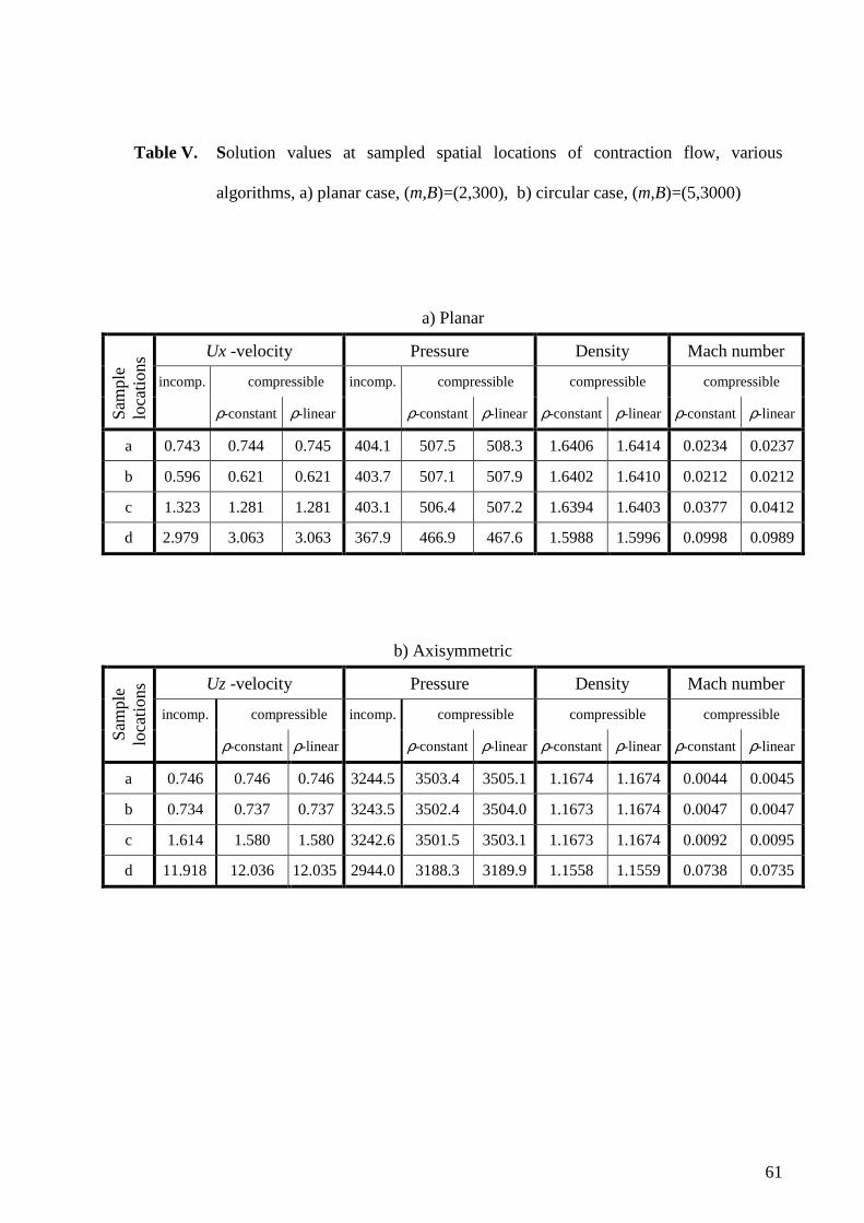
61
Table V. Solution values at sampled spatial locations of contraction flow, various
algorithms, a) planar case, (m,B)=(2,300), b) circular case, (m,B)=(5,3000)
a) Planar
Ux -velocity Pressure Density Mach number
incomp. compressible incomp. compressible compressible compressible
Sam
ple
loca
tions
ρ-constant ρ-linear ρ-constant ρ-linear ρ-constant ρ-linear ρ-constant ρ-linear
a 0.743 0.744 0.745 404.1 507.5 508.3 1.6406 1.6414 0.0234 0.0237
b 0.596 0.621 0.621 403.7 507.1 507.9 1.6402 1.6410 0.0212 0.0212
c 1.323 1.281 1.281 403.1 506.4 507.2 1.6394 1.6403 0.0377 0.0412
d 2.979 3.063 3.063 367.9 466.9 467.6 1.5988 1.5996 0.0998 0.0989
b) Axisymmetric
Uz -velocity Pressure Density Mach number
incomp. compressible incomp. compressible compressible compressible
Sam
ple
loca
tions
ρ-constant ρ-linear ρ-constant ρ-linear ρ-constant ρ-linear ρ-constant ρ-linear
a 0.746 0.746 0.746 3244.5 3503.4 3505.1 1.1674 1.1674 0.0044 0.0045
b 0.734 0.737 0.737 3243.5 3502.4 3504.0 1.1673 1.1674 0.0047 0.0047
c 1.614 1.580 1.580 3242.6 3501.5 3503.1 1.1673 1.1674 0.0092 0.0095
d 11.918 12.036 12.035 2944.0 3188.3 3189.9 1.1558 1.1559 0.0738 0.0735
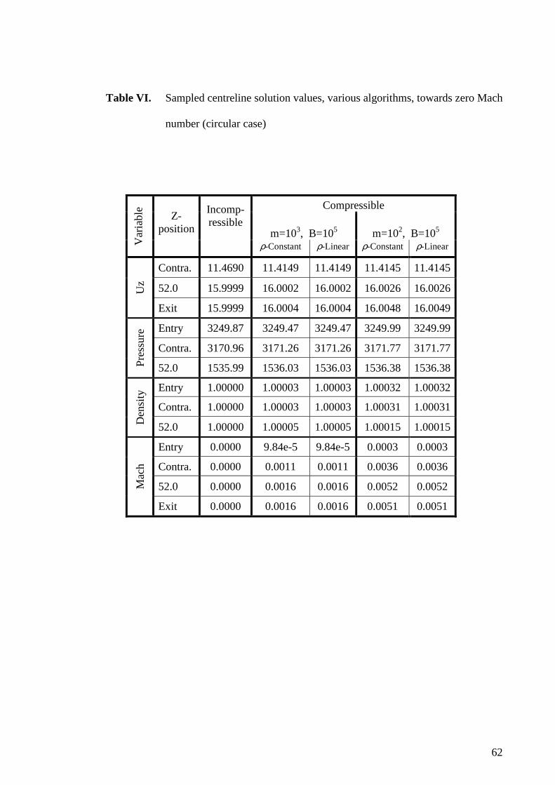
62
Table VI. Sampled centreline solution values, various algorithms, towards zero Mach
number (circular case)
Compressible
m=103, B=105 m=102, B=105
Var
iabl
e Z-
position
Incomp-ressible
ρ-Constant ρ-Linear ρ-Constant ρ-Linear
Contra. 11.4690 11.4149 11.4149 11.4145 11.4145
52.0 15.9999 16.0002 16.0002 16.0026 16.0026 Uz
Exit 15.9999 16.0004 16.0004 16.0048 16.0049
Entry 3249.87 3249.47 3249.47 3249.99 3249.99
Contra. 3170.96 3171.26 3171.26 3171.77 3171.77
Pre
ssur
e
52.0 1535.99 1536.03 1536.03 1536.38 1536.38
Entry 1.00000 1.00003 1.00003 1.00032 1.00032
Contra. 1.00000 1.00003 1.00003 1.00031 1.00031
Den
sity
52.0 1.00000 1.00005 1.00005 1.00015 1.00015
Entry 0.0000 9.84e-5 9.84e-5 0.0003 0.0003
Contra. 0.0000 0.0011 0.0011 0.0036 0.0036
52.0 0.0000 0.0016 0.0016 0.0052 0.0052 Mac
h
Exit 0.0000 0.0016 0.0016 0.0051 0.0051


