
Computational Investigation of Feature Extraction and Image
Organization
DISSERTATION
Presented in Partial Fulfillment of the Requirements for
the Degree Doctor of Philosophy in the
Graduate School of The Ohio State University
By
Xiuwen Liu, B.Eng., M.S., M.S.
* * * * *
The Ohio State University
1999
Dissertation Committee:
Prof. DeLiang L. Wang, Adviser
Prof. Song-Chun Zhu
Prof. Anton F. Schenk
Prof. Alan J. Saalfeld
Approved by
Adviser
Department of Computerand Information Science

c© Copyright by
Xiuwen Liu
1999
ABSTRACT
This dissertation investigates computational issues of feature extraction and im-
age organization at different levels. Boundary detection and segmentation are studied
extensively for range, intensity, and texture images. We developed a range image seg-
mentation system using a LEGION network based on a similarity measure consisting
of estimated surface properties. We propose a nonlinear smoothing algorithm through
local coupling structures, which exhibits distinctive temporal properties such as quick
convergence.
We propose spectral histograms, consisting of marginal distributions of a chosen
bank of filters, as a generic feature vector based on that early steps of human visual
processing can be modeled using local spatial/frequency representations. Spectral
histograms are studied extensively in texture modeling, classification, and segmenta-
tion. Experiments in texture synthesis and classification demonstrate that spectral
histograms provide a sufficient and unified feature in capturing perceptual appearance
of textures. Spectral histograms improve significantly the classification performance
for challenging texture images. We also propose a model for texture discrimination
based on spectral histograms which matches existing psychophysical data. A new en-
ergy functional for image segmentation is proposed. With given regional features, an
iterative and deterministic algorithm for segmentation is derived. Satisfactory results
ii

are obtained for natural texture images using spectral histograms. We also devel-
oped a novel algorithm which automatically identifies homogeneous texture features
from input images. By incorporating texture structures, we achieve accurate texture
boundary localization through a new distance measure. With extensive experiments,
we demonstrate that spectral histograms provide a generic feature which can be used
effectively to solve fundamental vision problems.
Based on a novel and biologically plausible boundary-pair representation, per-
ceptual organization is studied. A network is developed which can simulate many
perceptual phenomena through temporal dynamics. Boundary-pair representation
provides a unified explanation of edge- and surface-based representations.
A prototype system for automated feature extraction from remote sensing images
is developed. By combining the advantages of the learning-by-example method and a
locally coupled network, a generic feature extraction system is feasible. The system
is tested by extracting hydrographic features from large images of natural scenes.
iii

In memory of my parents, Fu-Lu Liu and She-Zi Liu, who taught me values and
knowledge silently.
iv

ACKNOWLEDGMENTS
I express my gratitude for my advisor, Prof. DeLiang Wang, who not only gener-
ously gives his time and energy, but also teaches me fundamental principles that are
essential for my scientific career. He not only gives me many scientific insights and
ideas, but also takes every chance to improve my skills in presentation and commu-
nication. I would also like to thank Prof. Song-Chun Zhu for sharing his time and
ideas with me. I benefit much from his computational thinking of vision problems.
I would like to thank my colleagues at Department of Computer and Information
Science, Department of Civil and Environmental Engineering and Geodetic Science,
and Center for Mapping for providing me an excellent environment for doing research.
I am especially grateful for Dr. John D. Bossler providing me opportunities to work
on challenging and yet fruitful problems. I would also like to thank Dr. Anton F.
Schenk, Dr. Alan J. Saalfeld, Dr. J. Raul Ramirez, Dr. Joseph C. Loon, Dr. Ke
Chen, Dr. Shannon Campbell, and many other faculty members and colleagues for
their strong support. I would also express my thanks to my colleagues in the Vision
Club at The Ohio State University, Dr. James Todd, Dr. Delwin Lindsey, and
Dr. Tjeerd Dijkstra, for stimulating discussions. Many thanks go to my teammates,
Dr. Erdogan Cesmeli, Mingying Wu, and Qiming Luo for their help and insightful
discussions. A Presidential Fellowship from The Ohio State University helped me
v

focus on my dissertation work in the last year of my Ph.D. study and is greatly
acknowledged.
I would like to thank my Lord Jesus Christ for His wonderful guidance, arrange-
ments, and opportunities He gives especially to me. I would like to express my sincere
gratitude for the strong support from my family. My mother-in-law takes a good care
of our family so that both my wife and I can focus on our studies. My wife Xujing pro-
vides a comfort and reliable home for me. Without her support and encouragement,
it would be impossible for me to finish my study. I thank my daughter Teng-Teng for
the enjoy we have together and for her support. I thank my families in China, my
sisters and brothers for their encouragement, understanding and support.
vi
VITA
August 14, 1966 . . . . . . . . . . . . . . . . . . . . . . . . . . . . Born - Hebei Province, China
July, 1989 . . . . . . . . . . . . . . . . . . . . . . . . . . . . . . . . . . B.Eng. Computer Science,Tsinghua University, Beijing, China
August, 1989 - February, 1993 . . . . . . . . . . . . . . Assistant Lecturer,Tsinghua University, Beijing, China
March, 1995 . . . . . . . . . . . . . . . . . . . . . . . . . . . . . . . . M.S. Geodetic Science and Surveying,The Ohio State University
June, 1996 . . . . . . . . . . . . . . . . . . . . . . . . . . . . . . . . . .M.S. Computer & Information Science,The Ohio State University
PUBLICATIONS
Journal Articles
X. Liu and J. R. Ramirez, “Automated vectorization and labeling of very largehypsographic map images using a contour graph.” Surveying and Land InformationSystems, vol. 57(1), pp. 5-10, 1997.
X. Liu and D. L. Wang, “Range image segmentation using an oscillatory network.”IEEE Transactions on Neural Networks, vol. 10(3), pp. 564-573, 1999.
X. Liu, D. L. Wang, and J. R. Ramirez, “Boundary detection by contextual nonlinearsmoothing.” Pattern Recognition, 1999.
Conference Papers
Y. Li, B. Zhang, and X. Liu, “A robust motion planner for assembly robots.” InProceedings of the IEEE International Conference on Robotics and Automation, vol.3, p. 1016, 1993.
vii
X. Liu and D. L. Wang, “Range image segmentation using an oscillatory network.”In Proceedings of the 1997 IEEE International Conference on Neural Networks, vol.3, pp. 1656-1660, 1997.
J. J. Loomis, X. Liu, Z. Ding, K. Fujimura, M. L. Evans, and H. Ishikawa, “Visualiza-tion of plant growth.” In Proceedings of the 1997 IEEE Conference on Visualization,pp. 475-478, 1997.
X. Liu and J. R. Ramirez, “Automatic extraction of hydrographic features in digitalorthophoto images.” In Proceedings of GIS/LIS’1997, pp. 365-373, 1997.
X. Liu, D. L. Wang, and J. R. Ramirez, “Extracting hydrographic objects fromsatellite images using a two-layer neural network.” In Proceedings of the 1998 Inter-national Joint Conference on Neural Networks, vol. 2, pp. 897-902, 1998.
X. Liu, D. L. Wang, and J. R. Ramirez, “A two-layer neural network for robust imagesegmentation and its application in revising hydrographic features.” InternationalArchives of Photogrammetry and Remote Sensing, vol. 32, part 3/1, 464-472, 1998.
X. Liu, D. L. Wang, and J. R. Ramirez, “Oriented Statistical Nonlinear SmoothingFilter.” In Proceedings of the 1998 International Conference on Image Processing,vol. 2, pp. 848-852, 1998.
X. Liu, “A prototype system for extracting hydrographic regions from Digital Or-thophoto Quadrangle images.” In Proceedings of GIS/LIS’1998, pp. 382-393, 1998.
X. Liu and D. L. Wang, “A boundary-pair representation for perception modeling.”In Proceedings of the 1999 International Joint Conference on Neural Networks, 1999.
X. Liu and D. L. Wang, “Modeling perceptural organization using temporal dynam-ics.” In Proceedings of the 1999 International Joint Conference on Neural Networks,1999.
Technical Report
J. J. Loomis, Z. Ding, X. Liu, K. Fujimura, and H. Ishikawa, “Flexible ObjectReconstruction from Temporal Image Series.” Technical Report OSU-CISRC-5/96-TR30, Department of Computer and Information Science, The Ohio State University,1996.
viii
X. Liu and D. L. Wang, “Range Image Segmentation Using a LEGION Network.”Technical Report OSU-CISRC-10/96-TR49, Department of Computer and Informa-tion Science, The Ohio State University, 1996.
X. Liu, D. L. Wang, and J. R. Ramirez, “Boundary Detection by Contextual Non-linear Smoothing.” Technical Report OSU-CISRC-7/98-TR21, Department of Com-puter and Information Science, The Ohio State University, 1998.
K. Chen, D. L. Wang, and X. Liu, “Weight adaptation and oscillatory correlationfor image segmentation.” Technical Report OSU-CISRC-8/98-TR37, Department ofComputer and Information Science, The Ohio State University, 1998.
X. Liu, K. Chen, and D. L. Wang, “Extraction of hydrographic regions from re-mote sensing images using an oscillator network with weight adaptation.” TechnicalReport OSU-CISRC-4/99-TR12, Department of Computer and Information Science,The Ohio State University, 1999.
FIELDS OF STUDY
Major Field: Computer and Information Science
Studies in:
Perception and Neurodynamics Prof. DeLiang L. WangMachine Vision Prof. Song-Chun ZhuDigital Photogrammetry Prof. Anton F. SchenkGeographic Information Systems Prof. Alan J. Saalfeld
ix
TABLE OF CONTENTS
Page
Abstract . . . . . . . . . . . . . . . . . . . . . . . . . . . . . . . . . . . . . . . ii
Dedication . . . . . . . . . . . . . . . . . . . . . . . . . . . . . . . . . . . . . . iv
Acknowledgments . . . . . . . . . . . . . . . . . . . . . . . . . . . . . . . . . . v
Vita . . . . . . . . . . . . . . . . . . . . . . . . . . . . . . . . . . . . . . . . . vii
List of Tables . . . . . . . . . . . . . . . . . . . . . . . . . . . . . . . . . . . . xiii
List of Figures . . . . . . . . . . . . . . . . . . . . . . . . . . . . . . . . . . . xiv
Chapters:
1. Introduction . . . . . . . . . . . . . . . . . . . . . . . . . . . . . . . . . . 1
1.1 Motivations . . . . . . . . . . . . . . . . . . . . . . . . . . . . . . . 11.2 Thesis Overview . . . . . . . . . . . . . . . . . . . . . . . . . . . . 6
2. Range Image Segmentation Using a Relaxation Oscillator Network . . . . 9
2.1 Introduction . . . . . . . . . . . . . . . . . . . . . . . . . . . . . . 102.2 Overview of the LEGION Dynamics . . . . . . . . . . . . . . . . . 13
2.2.1 Single Oscillator Model . . . . . . . . . . . . . . . . . . . . 132.2.2 Emergent Behavior of LEGION Networks . . . . . . . . . . 15
2.3 Similarity Measure for Range Images . . . . . . . . . . . . . . . . 202.4 Experimental Results . . . . . . . . . . . . . . . . . . . . . . . . . 25
2.4.1 Parameter Selection . . . . . . . . . . . . . . . . . . . . . . 252.4.2 Results . . . . . . . . . . . . . . . . . . . . . . . . . . . . . 262.4.3 Comparison with Existing Approaches . . . . . . . . . . . . 33
2.5 Discussions . . . . . . . . . . . . . . . . . . . . . . . . . . . . . . . 35
x

2.5.1 Biological Plausibility of the Network . . . . . . . . . . . . . 352.5.2 Comparison with Pulse-Coupled Neural Networks . . . . . . 362.5.3 Further Research Topics . . . . . . . . . . . . . . . . . . . . 38
3. Boundary Detection by Contextual Nonlinear Smoothing . . . . . . . . . 40
3.1 Introduction . . . . . . . . . . . . . . . . . . . . . . . . . . . . . . 413.2 Contextual Nonlinear Smoothing Algorithm . . . . . . . . . . . . . 45
3.2.1 Design of the Algorithm . . . . . . . . . . . . . . . . . . . . 453.2.2 A Generic Nonlinear Smoothing Framework . . . . . . . . . 49
3.3 Analysis . . . . . . . . . . . . . . . . . . . . . . . . . . . . . . . . 513.3.1 Theoretical Results . . . . . . . . . . . . . . . . . . . . . . . 513.3.2 Numerical Simulations . . . . . . . . . . . . . . . . . . . . . 54
3.4 Experimental Results . . . . . . . . . . . . . . . . . . . . . . . . . 583.4.1 Results of the Proposed Algorithm . . . . . . . . . . . . . . 583.4.2 Comparison with Nonlinear Smoothing Algorithms . . . . . 65
3.5 Conclusions . . . . . . . . . . . . . . . . . . . . . . . . . . . . . . 73
4. Spectral Histogram: A Generic Feature for Images . . . . . . . . . . . . . 75
4.1 Introduction . . . . . . . . . . . . . . . . . . . . . . . . . . . . . . 764.2 Spectral Histograms . . . . . . . . . . . . . . . . . . . . . . . . . . 82
4.2.1 Properties of Spectral Histograms . . . . . . . . . . . . . . . 854.2.2 Choice of Filters . . . . . . . . . . . . . . . . . . . . . . . . 85
4.3 Texture Synthesis . . . . . . . . . . . . . . . . . . . . . . . . . . . 874.3.1 Comparison with Heeger and Bergen’s Algorithm . . . . . . 96
4.4 Texture Classification . . . . . . . . . . . . . . . . . . . . . . . . . 1014.4.1 Classification at Fixed Scales . . . . . . . . . . . . . . . . . 1044.4.2 Classification at Different Scales . . . . . . . . . . . . . . . 1054.4.3 Image Classification . . . . . . . . . . . . . . . . . . . . . . 1084.4.4 Training Samples and Generalization . . . . . . . . . . . . . 1114.4.5 Comparison with Existing Approaches . . . . . . . . . . . . 113
4.5 Content-based Image Retrieval . . . . . . . . . . . . . . . . . . . . 1154.6 Comparison of Statistic Features . . . . . . . . . . . . . . . . . . . 1214.7 A Model for Texture Discrimination . . . . . . . . . . . . . . . . . 1244.8 Conclusions . . . . . . . . . . . . . . . . . . . . . . . . . . . . . . 129
5. Image Segmentation Using Spectral Histograms . . . . . . . . . . . . . . 131
5.1 Introduction . . . . . . . . . . . . . . . . . . . . . . . . . . . . . . 1315.2 Formulation of Energy Functional for Segmentation . . . . . . . . 1345.3 Algorithms for Segmentation . . . . . . . . . . . . . . . . . . . . . 135
xi

5.4 Segmentation with Given Region Features . . . . . . . . . . . . . . 1395.4.1 Segmentation at a Fixed Integration Scale . . . . . . . . . . 1405.4.2 Segmentation with Multiple Scales . . . . . . . . . . . . . . 1505.4.3 Region-of-interest Extraction . . . . . . . . . . . . . . . . . 153
5.5 Automated Seed Selection . . . . . . . . . . . . . . . . . . . . . . 1565.6 Localization of Texture Boundaries . . . . . . . . . . . . . . . . . 1605.7 Discussions . . . . . . . . . . . . . . . . . . . . . . . . . . . . . . . 1645.8 Conclusions . . . . . . . . . . . . . . . . . . . . . . . . . . . . . . 168
6. Perceptual Organization Based on Temporal Dynamics . . . . . . . . . . 169
6.1 Introduction . . . . . . . . . . . . . . . . . . . . . . . . . . . . . . 1706.2 Figure-Ground Segregation Network . . . . . . . . . . . . . . . . . 172
6.2.1 Boundary-Pair Representation . . . . . . . . . . . . . . . . 1726.2.2 Incorporation of Gestalt Rules . . . . . . . . . . . . . . . . 1756.2.3 Temporal Properties of the Network . . . . . . . . . . . . . 177
6.3 Surface Completion . . . . . . . . . . . . . . . . . . . . . . . . . . 1786.4 Experimental Results . . . . . . . . . . . . . . . . . . . . . . . . . 1796.5 Conclusions . . . . . . . . . . . . . . . . . . . . . . . . . . . . . . 184
7. Extraction of Hydrographic Regions from Remote Sensing Images Usingan Oscillator Network with Weight Adaptation . . . . . . . . . . . . . . 188
7.1 Introduction . . . . . . . . . . . . . . . . . . . . . . . . . . . . . . 1897.2 Weight Adaptation . . . . . . . . . . . . . . . . . . . . . . . . . . 1937.3 Automated Seed Selection . . . . . . . . . . . . . . . . . . . . . . 2007.4 Experimental Results . . . . . . . . . . . . . . . . . . . . . . . . . 202
7.4.1 Parameter Selection . . . . . . . . . . . . . . . . . . . . . . 2037.4.2 Synthetic Image . . . . . . . . . . . . . . . . . . . . . . . . 2037.4.3 Hydrographic Region Extraction from DOQQ Images . . . . 204
7.5 Discussions . . . . . . . . . . . . . . . . . . . . . . . . . . . . . . . 218
8. Conclusions and Future Work . . . . . . . . . . . . . . . . . . . . . . . . 221
8.1 Contributions of Dissertation . . . . . . . . . . . . . . . . . . . . . 2218.2 Future Work . . . . . . . . . . . . . . . . . . . . . . . . . . . . . . 222
8.2.1 Correspondence Through Spectral Histograms . . . . . . . . 2228.2.2 Integration of Bottom-up and Top-down Approaches . . . . 2238.2.3 Psychophysical Experiments . . . . . . . . . . . . . . . . . . 227
8.3 Concluding Remarks . . . . . . . . . . . . . . . . . . . . . . . . . . 228
Bibliography . . . . . . . . . . . . . . . . . . . . . . . . . . . . . . . . . . . . 229
xii

LIST OF TABLES
Table Page
3.1 Quantitative comparison of boundary detection results shown in Figure3.15. . . . . . . . . . . . . . . . . . . . . . . . . . . . . . . . . . . . . 71
3.2 Quantitative comparison of boundary detection results shown in Figure3.16. . . . . . . . . . . . . . . . . . . . . . . . . . . . . . . . . . . . . 71
4.1 L1-norm distance of the spectral histograms and RMS distance betweenimages. . . . . . . . . . . . . . . . . . . . . . . . . . . . . . . . . . . . 99
4.2 Classification errors of methods shown in [108] and our method . . . 115
4.3 Comparison of texture discrimination measures . . . . . . . . . . . . 128
7.1 Comparison of error rates using neural network classification and theproposed method. . . . . . . . . . . . . . . . . . . . . . . . . . . . . . 205
xiii

LIST OF FIGURES
Figure Page
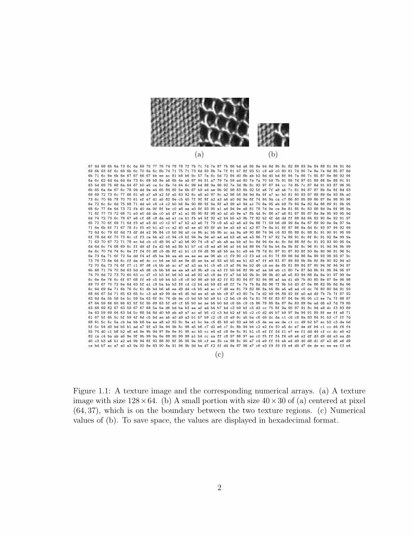
1.1 A texture image and the corresponding numerical arrays. (a) A textureimage with size 128× 64. (b) A small portion with size 40× 30 of (a)centered at pixel (64, 37), which is on the boundary between the twotexture regions. (c) Numerical values of (b). To save space, the valuesare displayed in hexadecimal format. . . . . . . . . . . . . . . . . . . 2
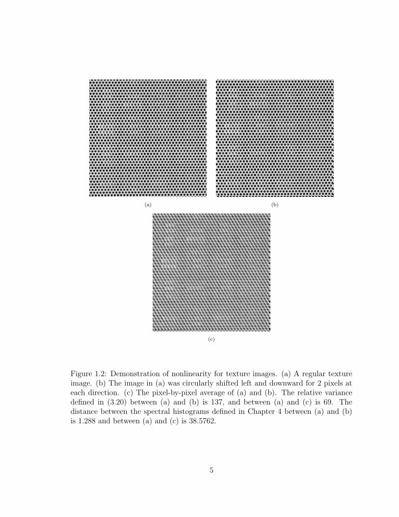
1.2 Demonstration of nonlinearity for texture images. (a) A regular textureimage. (b) The image in (a) was circularly shifted left and downwardfor 2 pixels at each direction. (c) The pixel-by-pixel average of (a) and(b). The relative variance defined in (3.20) between (a) and (b) is 137,and between (a) and (c) is 69. The distance between the spectral his-tograms defined in Chapter 4 between (a) and (b) is 1.288 and between(a) and (c) is 38.5762. . . . . . . . . . . . . . . . . . . . . . . . . . . 5
2.1 A stable limit cycle for a single relaxation oscillator. The thick solidline represents the limit cycle and thin solid lines stand for nullclines.Arrows are used to indicate the different traveling speed, resultingfrom fast and slow time scales. The following parameter values areused: ε = 0.02, β = 0.1, γ = 3.0, and a constant stimulus I = 1.0. . . 15
2.2 The temporal activities of the excitatory unit of a single oscillator fordifferent γ values. Other parameters are same as for Figure 2.1. (a)γ = 3.0. (b) γ = 40.0. . . . . . . . . . . . . . . . . . . . . . . . . . . . 16
2.3 Architecture of a two-dimensional LEGION network with eight-nearestneighbor coupling. An oscillator is indicated by an empty ellipse, andthe global inhibitor is indicated by a filled circle. . . . . . . . . . . . . 19
xiv

2.4 Illustration of LEGION dynamics. (a) An input image consisting ofseven geometric objects, with 40× 40 pixels. (b) The corrupted imageof (a) by adding 10which is presented to a 40×40 LEGION network. (c)A snapshot of the network activity at the beginning. (d)-(j) Subsequentsnapshots of the network activity. In (c)-(j), the grayness of a pixel isproportional to the corresponding oscillator’s activity and black pixelsrepresent oscillators in the active phase. The parameter values for thissimulation are following: ε = 0.02, β = 0.1, γ = 20.0, θx = −0.5,θp = 7.0, θz = 0.1, θ = 0.8, and Wz = 2.0. . . . . . . . . . . . . . . . . 21
2.5 Temporal evolution of the LEGION network. The upper seven plotsshow the combined temporal activities of the seven oscillator blocksrepresenting the corresponding geometric objects. The eighth plotshows the temporal activities of all the stimulated oscillators whichcorrespond to the background. The bottom one shows the temporalactivity of the global inhibitor. The simulation took 20,000 integrationsteps using a fourth-order Runge-Kutta method to solve differentialequations. . . . . . . . . . . . . . . . . . . . . . . . . . . . . . . . . . 22
2.6 Segmentation result of the LEGION network for the range image of acolumn. (a) The input range image. (b) The background region. (c)-(f) The four segmented regions. (g) The overall segmentation resultrepresented by a gray map. (h) The corresponding intensity image. (i)The 3-D construction model. As in Figure 2.4, black pixels in (b)-(f)represent oscillators that are in the active phase. . . . . . . . . . . . . 28
2.7 Segmentation results of the LEGION network for range images. Ineach row, the left frame shows the input range image, the middle oneshows the segmentation result represented by a gray map, and the rightone shows the 3-D construction model for comparison purposes. . . . 30
2.8 Segmentation results of the LEGION network for several more rangeimages. See the caption of Figure 2.7 for arrangement. . . . . . . . . 31
2.9 Two examples with thin regions. The global inhibition and potentialthreshold are tuned to get the results shown here. See the caption ofFigure 2.7 for arrangement. . . . . . . . . . . . . . . . . . . . . . . . 32
xv

2.10 A hierarchy obtained from multiscale segmentation. The top is theinput range image and each segmented region is further segmented byincreasing the level of global inhibition. As in Figure 2.6, black pixelsrepresent active oscillators, corresponding to the popped up region.See Figure 2.6(i) for the corresponding 3-D model. . . . . . . . . . . . 39
3.1 An example with non-uniform boundary gradients and substantialnoise. (a) A noise-free synthetic image. Gray values in the image: 98for the left ‘[’ region, 138 for the square, 128 for the central oval, and 158for the right ‘]’ region. (b) A noisy version of (a) with Gaussian noiseof σ = 40. (c) Local gradient map of (b) using the Sobel operators.(d)-(f) Smoothed images from an anisotropic diffusion algorithm [106]at 50, 100, and 1000 iterations. (g)-(i) Corresponding edge maps of(d)-(f) respectively using the Sobel edge detector. . . . . . . . . . . . 44
3.2 Illustration of the coupling structure of the proposed algorithm. (a)Eight oriented windows and a fully connected window defined on a3 x 3 neighborhood. (b) A small synthetic image patch of 6 x 8 inpixels. (c) The resulting coupling structure for (b). There is a directededge from (i1, j1) to a neighbor (i0, j0) if and only if (i1, j1) contributesto the smoothing of (i0, j0) according to equations (3.12) and (3.9).Each circle represents a pixel, where the inside color is proportionalto the gray value of the corresponding pixel. Ties in (3.9) are brokenaccording to left-right and top-down preference of the oriented windowsin (a). . . . . . . . . . . . . . . . . . . . . . . . . . . . . . . . . . . . 53
3.3 Temporal behavior of the proposed algorithm with respect to theamount of noise. Six noisy images are obtained by adding zero-meanGaussian noise with σ of 5, 10, 20, 30, 40, and 60, respectively, to thenoise-free image shown in Figure 3.1(a). The plot shows the deviationfrom the ground truth image with respect to iterations of the noise-freeimage and six noisy images. . . . . . . . . . . . . . . . . . . . . . . . 56
3.4 Relative variance of the proposed algorithm for the noise-free imageshown in Figure 3.1(a) and four noisy images with Gaussian noise ofzero-mean and σ of 5, 20, 40 and 60, respectively. . . . . . . . . . . . 57
3.5 Relative variance of the proposed algorithm for real images shown inFigure 3.9-3.12. . . . . . . . . . . . . . . . . . . . . . . . . . . . . . . 58
xvi
3.6 The oriented bar-like windows used throughout this chapter for syn-thetic and real images. The size of each kernel is approximately 3 x 10in pixels. . . . . . . . . . . . . . . . . . . . . . . . . . . . . . . . . . . 59
3.7 The smoothed images at the 11th iteration and detected boundariesfor three synthetic images by adding specified Gaussian noise to thenoise-free image shown in Figure 3.1(a). Top row shows the inputimages, middle the smoothed image at the 11th iteration, and bottomthe detected boundaries using the Sobel edge detector. (a) Gaussiannoise with σ = 10. (b) Gaussian noise with σ = 40. (c) Gaussian noisewith σ = 60. . . . . . . . . . . . . . . . . . . . . . . . . . . . . . . . . 61
3.8 The smoothed image at the 11th iteration and detected boundaries fora synthetic image with corners. (a) Input image. (b) Smoothed image.(c) Boundaries detected. . . . . . . . . . . . . . . . . . . . . . . . . . 62
3.9 The smoothed image at the 11th iteration and detected boundaries fora grocery store advertisement. Details are smoothed out while majorboundaries and junctions are preserved accurately. (a) Input image.(b) Smoothed image. (c) Boundaries detected. . . . . . . . . . . . . . 62
3.10 The smoothed image at the 11th iteration and detected boundaries fora natural satellite image with several land use patterns. The bound-aries between different regions are formed from noisy segments due tothe coupling structure. (a) Input image. (b) Smoothed image. (c)Boundaries detected. . . . . . . . . . . . . . . . . . . . . . . . . . . . 63
3.11 The smoothed image at the 11th iteration and detected boundaries fora woman image. While the boundaries between large features are pre-served and detected, detail features such as facial features are smoothedout. (a) Input image. (b) Smoothed image. (c) Boundaries detected. 64
3.12 The smoothed image at the 11th iteration and detected boundaries fora texture image. The boundaries between different textured regionsare formed while details due to textures are smoothed out. (a) Inputimage. (b) Smoothed image. (c) Boundaries detected. . . . . . . . . . 65
xvii
3.13 Deviations from the ground truth image for the four nonlinear smooth-ing methods. Dashed line: The SUSAN filter [117]; Dotted line: ThePerona-Malik model [105]; Dash-dotted line: The Weickert model ofedge enhancing anisotropic diffusion [137]; Solid line: The proposedalgorithm. . . . . . . . . . . . . . . . . . . . . . . . . . . . . . . . . . 67
3.14 Relative variance of the four nonlinear smoothing methods. Dashedline: The SUSAN filter [117]; Dotted line: The Perona-Malik diffusionmodel [105]; Dash-dotted line: The Weickert model [137]; Solid line:The proposed algorithm. . . . . . . . . . . . . . . . . . . . . . . . . . 68
3.15 Smoothing results and detected boundaries of the four nonlinear meth-ods for a synthetic image shown in Figure 3.7(a). Here noise is not largeand all of the methods perform well in preserving boundaries. . . . . 70
3.16 Smoothing results and detected boundaries of the four nonlinear meth-ods for a synthetic image with substantial noise shown in Figure 3.7(b).The proposed algorithm generates sharper and better connectedboundaries than the other three methods. . . . . . . . . . . . . . . . 72
3.17 Smoothing results and detected boundaries of a natural scene satelliteimage shown in Figure 3.10. Smoothed image of the proposed algo-rithm is at the 11th iteration while smoothed images of the other threemethods are chosen manually. While the other three methods gener-ate similar fragmented boundaries, the proposed algorithm forms theboundaries between different regions due to its coupling structure. . . 72
4.1 Basis functions of Fourier transform in time and frequency domainswith their Fourier transforms. (a) An impulse and its Fourier trans-form. (b) A sinusoid function and its Fourier transform. . . . . . . . . 79
4.2 A texture image with its Gabor filter response. (a) Input texture image.(b) A Gabor filter, which is truncated to save computation. (c) Thefilter response obtained through convolution. . . . . . . . . . . . . . . 81
4.3 A texture image and its spectral histograms. (a) Input image. (b) AGabor filter. (c) The histogram of the filter. (d) Spectral histogramsof the image. There are eight filters including intensity filter, gradientfilters Dxx and Dyy, four LoG filters with T =
√2/2, 1, 2, and 4, and
a Gabor filter Gcos(12, 150). There are 8 bins in the histograms ofintensity and gradient filters and 11 bins for the other filters. . . . . . 84
xviii

4.4 Gibbs sampler for texture synthesis. . . . . . . . . . . . . . . . . . . . 88
4.5 Texture image synthesis by matching observed statistics. (a) Observedtexture image. (b) Initial image. (c) Synthesized image after 14 sweeps.(d) The total matched error with respect to sweeps. . . . . . . . . . . 90
4.6 Temporal evolution of a selected filter for texture synthesis. (a) AGabor filter. (b) The histograms of the Gabor filter. Dotted line -observed histogram, which is covered by the histogram after 14 sweeps;dashed line - initial histogram; dash-dotted line - histogram after 2sweeps. solid line - histogram after 14 sweeps. (c) The error of thechosen filter with respect to the sweeps. (d) The error between theobserved histogram and the synthesized one after 14 sweeps. Here theerror is multiplied by 1000. . . . . . . . . . . . . . . . . . . . . . . . . 91
4.7 More texture synthesis examples. Left column shows the observedimages and right column shows the synthesized image within 15 sweeps.In (b), due to local minima, there are local regions which are notperceptually similar to the observed image. . . . . . . . . . . . . . . . 92
4.8 Real texture images of regular patterns with synthesized images after20 sweeps. (a) An image of a leather surface. The total matched errorafter 20 sweeps is 0.082. (b) An image of a pressed calf leather surface.The total matched error after 20 sweeps is 0.064. . . . . . . . . . . . 94
4.9 Texture synthesis for an image with different regions. (a) The observedtexture image. This image is not a homogeneous texture image andconsists mainly of two homogeneous regions. (b) The initial image.(c) Synthesized image after 100 sweeps. Even though the spectral his-togram of each filter is matched well, compared to other images, theerror is still large. Especially for the intensity filter, the error is stillabout 7.44 %. The synthesized image is perceptually similar to theobserved image except the geometrical relationships among the homo-geneous regions. (d) The matched error with respect to the sweeps.Due to that the observed image is not homogeneous, the synthesisalgorithm converges slower compared with Figure 4.5(d). . . . . . . . 95
4.10 A synthesis example for a synthetic texton image. (a) The originalsynthetic texton image with size 128× 128. (b) The synthesized imagewith size 256× 256. . . . . . . . . . . . . . . . . . . . . . . . . . . . . 96
xix

4.11 A synthesis example for an image consisting of two regions. (a) Theoriginal synthetic image with size 128×128, consisting of two intensityregions. (b) The synthesized image with size 256× 256. . . . . . . . . 97
4.12 A synthesis example for a face image. (a) Lena image with size 347×334. (b) The synthesized image with size 256× 256. . . . . . . . . . . 97
4.13 The synthesized images of the 40 texture images shown in Figure 4.16.Here same filters and cooling schedule are used for all the images. . . 98
4.14 Synthesized images from different initial images for the texture imageshown in Figure 4.3(a). (a)-(c) Left column is the initial image andright column is the synthesized image after 20 sweeps. (d) The matchederror with respect to the number of sweeps. . . . . . . . . . . . . . . 100
4.15 Synthesized images from Heeger and Bergen’s aglorithm and thematched spectral histogram error for the image shown in Figure 4.3(a).(a) Synthesized image at 3 iterations. (b) Synthesized image at 10iterations. (c) Synthesized image at 100 iterations. (d) The L1-normerror of the observed spectral histogram and the synthesized one. . . 102
4.16 Forty texture images used in the classification experiments. The inputimage size is 256× 256. . . . . . . . . . . . . . . . . . . . . . . . . . . 103
4.17 The divergence between the feature vector of each image in the textureimage database shown in Figure 4.16. (a) The cross-divergence matrixshown in numerical values. (b) The numerical values are displayed asan image. . . . . . . . . . . . . . . . . . . . . . . . . . . . . . . . . . 106
4.18 (a) The classification error for each image in the texture database alongwith the ratio between the maximum and minimum divergence shownin (b) and (c) respectively. (b) The maximum divergence of spectralhistogram from the feature vector of each image. (c) The minimumdivergence between each image and the other ones. . . . . . . . . . . 107
4.19 The classification error of the texture database with respect to the scalefor feature extraction. . . . . . . . . . . . . . . . . . . . . . . . . . . . 108
xx
4.20 (a) Image “Hexholes-2” from the texture database. (b) The classi-fication error rate for the image. (c) The ratio between maximumdivergence and minimum cross divergence with respect to scales. . . . 109
4.21 (a) Image “Woolencloth-2” from the texture database. (b) The clas-sification error rate for the image. (c) The ratio between maximumdivergence and minimum cross divergence with respect to scales. . . . 110
4.22 (a) A texture image consisting of five texture regions from the tex-ture database. (b) Classification result using spectral histograms. (c)Divergence between spectral histograms and the feature vector of theassigned texture image. (d) The ground truth segmentation of theimage. (e) Misclassified pixels, shown in black. . . . . . . . . . . . . . 112
4.23 (a) The classification error for each image in the database at integrationscale 35×35. (b) The classification error at different integration scales.In both cases, solid line – training is done using half of the samples;dashed line – training is done using all the samples. . . . . . . . . . . 113
4.24 The classification error with respect to the ratio of testing samples totraining samples. Solid line – integration scale 35 × 35; dashed line –integration scale 23× 23. . . . . . . . . . . . . . . . . . . . . . . . . 114
4.25 A group of 10 texture images used in [108]. Each image is 256× 256. 116
4.26 A group of 10 texture images used in [108]. Each image is 256× 256. 117
4.27 Image retrieval result from a 100-image database using a given im-age patch based on spectral histograms. (a) Input image patch withsize 35 × 35. (b) The sorted matched error for the 100 images in thedatabase. (c) The first nine image with smallest errors. . . . . . . . . 119
4.28 Image retrieval result from a 100-image database using a given im-age patch based on spectral histograms. (a) Input image patch withsize 53 × 53. (b) The sorted matched error for the 100 images in thedatabase. (c) The first nine image with smallest errors. . . . . . . . . 120
xxi
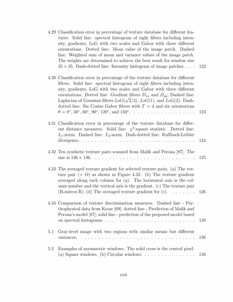
4.29 Classification error in percentage of texture database for different fea-tures. Solid line: spectral histogram of eight filters including inten-sity, gradients, LoG with two scales and Gabor with three differentorientations. Dotted line: Mean value of the image patch. Dashedline: Weighted sum of mean and variance values of the image patch.The weights are determined to achieve the best result for window size35× 35. Dash-dotted line: Intensity histogram of image patches. . . . 122
4.30 Classification error in percentage of the texture database for differentfilters. Solid line: spectral histogram of eight filters including inten-sity, gradients, LoG with two scales and Gabor with three differentorientations. Dotted line: Gradient filters Dxx and Dyy; Dashed line:Laplacian of Gaussian filters LoG(
√2/2), LoG(1), and LoG(2). Dash-
dotted line: Six Cosine Gabor filters with T = 4 and six orientationsθ = 0, 30, 60, 90, 120, and 150. . . . . . . . . . . . . . . . . . . 123
4.31 Classification error in percentage of the texture database for differ-ent distance measures. Solid line: χ2-square statistic. Dotted line:L1-norm. Dashed line: L2-norm. Dash-dotted line: Kullback-Leiblerdivergence. . . . . . . . . . . . . . . . . . . . . . . . . . . . . . . . . . 124
4.32 Ten synthetic texture pairs scanned from Malik and Perona [87]. Thesize is 136× 136. . . . . . . . . . . . . . . . . . . . . . . . . . . . . . 125
4.33 The averaged texture gradient for selected texture pairs. (a) The tex-ture pair (+ O) as shown in Figure 4.32. (b) The texture gradientaveraged along each column for (a). The horizontal axis is the col-umn number and the vertical axis is the gradient. (c) The texture pair(R-mirror-R). (d) The averaged texture gradient for (c). . . . . . . . 126
4.34 Comparison of texture discrimination measures. Dashed line - Psy-chophysical data from Krose [69]; dotted line - Prediction of Malik andPerona’s model [87]; solid line - prediction of the proposed model basedon spectral histograms. . . . . . . . . . . . . . . . . . . . . . . . . . . 128
5.1 Gray-level image with two regions with similar means but differentvariances. . . . . . . . . . . . . . . . . . . . . . . . . . . . . . . . . . 136
5.2 Examples of asymmetric windows. The solid cross is the central pixel.(a) Square windows. (b) Circular windows. . . . . . . . . . . . . . . . 138
xxii
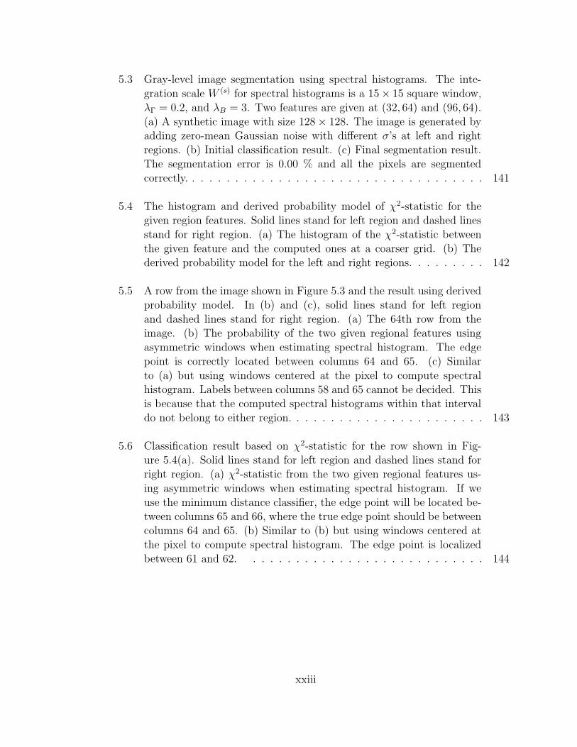
5.3 Gray-level image segmentation using spectral histograms. The inte-gration scale W (s) for spectral histograms is a 15× 15 square window,λΓ = 0.2, and λB = 3. Two features are given at (32, 64) and (96, 64).(a) A synthetic image with size 128× 128. The image is generated byadding zero-mean Gaussian noise with different σ’s at left and rightregions. (b) Initial classification result. (c) Final segmentation result.The segmentation error is 0.00 % and all the pixels are segmentedcorrectly. . . . . . . . . . . . . . . . . . . . . . . . . . . . . . . . . . . 141
5.4 The histogram and derived probability model of χ2-statistic for thegiven region features. Solid lines stand for left region and dashed linesstand for right region. (a) The histogram of the χ2-statistic betweenthe given feature and the computed ones at a coarser grid. (b) Thederived probability model for the left and right regions. . . . . . . . . 142
5.5 A row from the image shown in Figure 5.3 and the result using derivedprobability model. In (b) and (c), solid lines stand for left regionand dashed lines stand for right region. (a) The 64th row from theimage. (b) The probability of the two given regional features usingasymmetric windows when estimating spectral histogram. The edgepoint is correctly located between columns 64 and 65. (c) Similarto (a) but using windows centered at the pixel to compute spectralhistogram. Labels between columns 58 and 65 cannot be decided. Thisis because that the computed spectral histograms within that intervaldo not belong to either region. . . . . . . . . . . . . . . . . . . . . . . 143
5.6 Classification result based on χ2-statistic for the row shown in Fig-ure 5.4(a). Solid lines stand for left region and dashed lines stand forright region. (a) χ2-statistic from the two given regional features us-ing asymmetric windows when estimating spectral histogram. If weuse the minimum distance classifier, the edge point will be located be-tween columns 65 and 66, where the true edge point should be betweencolumns 64 and 65. (b) Similar to (b) but using windows centered atthe pixel to compute spectral histogram. The edge point is localizedbetween 61 and 62. . . . . . . . . . . . . . . . . . . . . . . . . . . . 144
xxiii

5.7 Gray-level image segmentation using spectral histograms. W (s) is a15× 15 square window, λΓ = 0.2, and λB = 5. Two features are givenat (32, 64) and (96, 45). (a) A synthetic image with size 128×128. Theimage is generated by adding zero-mean Gaussian noise with differentσ’s at the two different regions. Here the boundary is ’S’ shaped totest the segmentation algorithm in preserving boundaries. (b) Initialclassification result. (c) Final segmentation result. . . . . . . . . . . . 145
5.8 Texture image segmentation using spectral histograms. W (s) is a 29×29 square window, λΓ = 0.2, and λB = 2. Features are given at pixels(32, 32) and (96, 32). (a) A texture image consisting of two textureregions with size 128 × 64. (b) Initial classification result. (c) Finalsegmentation result. . . . . . . . . . . . . . . . . . . . . . . . . . . . 145
5.9 Texture image segmentation using spectral histograms. W (s) is a 29×29 square window, λΓ = 0.2, and λB = 3. (a) A texture image consist-ing of two texture regions with size 128 × 64. (b) Initial classificationresult. (c) Final segmentation result. . . . . . . . . . . . . . . . . . . 146
5.10 Texture image segmentation using spectral histograms. W (s) is a 35×35 square window, λΓ = 0.4, and λB = 3. Four features are given at(32, 32), (32, 96), (96, 32), and (96, 96). (a) A texture image consistingof four texture regions with size 128 × 128. (b) Initial classificationresult. (c) Final segmentation result. . . . . . . . . . . . . . . . . . . 147
5.11 Texture image segmentation using spectral histograms. W (s) is a 35×35 square window, λΓ = 0.4, and λB = 3. Four features are given at(32, 32), (32, 96), (96, 32), and (96, 96). (a) A texture image consistingof four texture regions with size 128 × 128. (b) Initial classificationresult. (c) Final segmentation result. . . . . . . . . . . . . . . . . . . 147
5.12 Texture image segmentation using spectral histograms. W (s) is a 29×29 square window, λΓ = 0.2, and λB = 3. Four features are given at(32, 32), (32, 96), (96, 32), and (96, 96). (a) A texture image consistingof four texture regions with size 128 × 128. (b) Initial classificationresult. (c) Final segmentation result. . . . . . . . . . . . . . . . . . . 148
xxiv
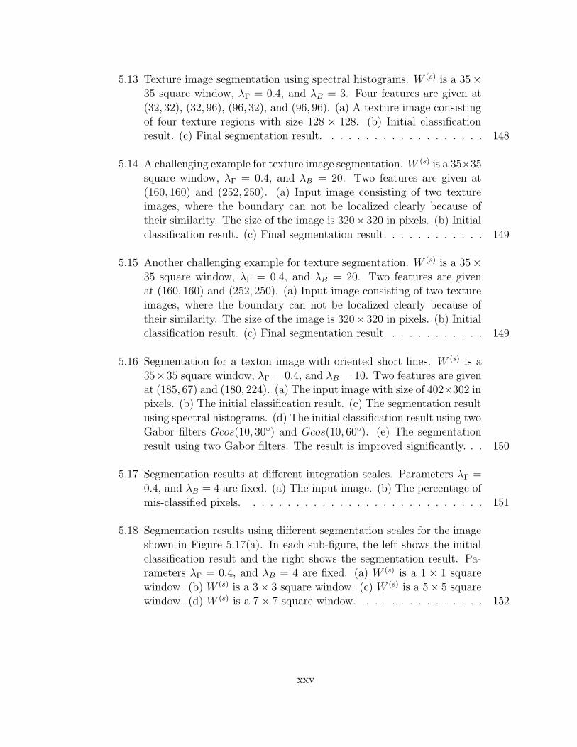
5.13 Texture image segmentation using spectral histograms. W (s) is a 35×35 square window, λΓ = 0.4, and λB = 3. Four features are given at(32, 32), (32, 96), (96, 32), and (96, 96). (a) A texture image consistingof four texture regions with size 128 × 128. (b) Initial classificationresult. (c) Final segmentation result. . . . . . . . . . . . . . . . . . . 148
5.14 A challenging example for texture image segmentation. W (s) is a 35×35square window, λΓ = 0.4, and λB = 20. Two features are given at(160, 160) and (252, 250). (a) Input image consisting of two textureimages, where the boundary can not be localized clearly because oftheir similarity. The size of the image is 320× 320 in pixels. (b) Initialclassification result. (c) Final segmentation result. . . . . . . . . . . . 149
5.15 Another challenging example for texture segmentation. W (s) is a 35×35 square window, λΓ = 0.4, and λB = 20. Two features are givenat (160, 160) and (252, 250). (a) Input image consisting of two textureimages, where the boundary can not be localized clearly because oftheir similarity. The size of the image is 320× 320 in pixels. (b) Initialclassification result. (c) Final segmentation result. . . . . . . . . . . . 149
5.16 Segmentation for a texton image with oriented short lines. W (s) is a35×35 square window, λΓ = 0.4, and λB = 10. Two features are givenat (185, 67) and (180, 224). (a) The input image with size of 402×302 inpixels. (b) The initial classification result. (c) The segmentation resultusing spectral histograms. (d) The initial classification result using twoGabor filters Gcos(10, 30) and Gcos(10, 60). (e) The segmentationresult using two Gabor filters. The result is improved significantly. . . 150
5.17 Segmentation results at different integration scales. Parameters λΓ =0.4, and λB = 4 are fixed. (a) The input image. (b) The percentage ofmis-classified pixels. . . . . . . . . . . . . . . . . . . . . . . . . . . . 151
5.18 Segmentation results using different segmentation scales for the imageshown in Figure 5.17(a). In each sub-figure, the left shows the initialclassification result and the right shows the segmentation result. Pa-rameters λΓ = 0.4, and λB = 4 are fixed. (a) W (s) is a 1 × 1 squarewindow. (b) W (s) is a 3× 3 square window. (c) W (s) is a 5× 5 squarewindow. (d) W (s) is a 7× 7 square window. . . . . . . . . . . . . . . 152
xxv

5.19 A texture image with a cheetah. The feature vector is calculated atpixel (247, 129) at scale 19 × 19, λΓ = 0.2, and λB = 2.5. To demon-strate the accuracy of the results, the classification and segmentationresults are embedded into the original image by lowering the intensityvalues of the background region by a factor of 2. (a) The input imagewith size 324× 486. (b) The initial classification result using 8 filters.(c) The final segmentation result using 8 filters. (d) The initial classifi-cation result using 6 filters consisting ofDxx, Dyy, LoG(
√2/2), LoG(1),
LoG(2) and LoG(3). (e) The final segmentation result correspondingto (d). . . . . . . . . . . . . . . . . . . . . . . . . . . . . . . . . . . . 154
5.20 An indoor image with a sofa. The feature vector is calculated at pixel(146, 169) at scale 35×35, λΓ = 0.2, and λB = 3. (a) Input image withsize 512× 512. (b) Initial classification result. (c) Final segmentationresult. (d) Segmentation result if we assume there is another regionfeature given at (223, 38). . . . . . . . . . . . . . . . . . . . . . . . . 155
5.21 Texture image segmentation with representative pixels identified auto-matically. W (s) is a 29 × 29 square window, W (a) is a 35 × 35 squarewindow, λC = 0.1, λA = 0.2, λB = 2.0, λΓ = 0.2, and TA = 0.08. (a)Input texture image, which is shown in Figure 5.8. (b) Initial classifica-tion result. Here the representative pixels are detected automatically.(c) Final segmentation result. . . . . . . . . . . . . . . . . . . . . . . 158
5.22 Texture image segmentation with representative pixels identified auto-matically. W (s) is a 29 × 29 square window, W (a) is a 43 × 43 squarewindow, λC = 0.4, λA = 0.4, λB = 5.0, λΓ = 0.4, and TA = 0.30.(a) Input texture image, which is shown in Figure 5.10. (b) Initialclassification result. Here the representative pixels are detected auto-matically. (c) Final segmentation result. . . . . . . . . . . . . . . . . 158
5.23 Texture image segmentation with representative pixels identified auto-matically. W (s) is a 29 × 29 square window, W (a) is a 43 × 43 squarewindow, λC = 0.1, λA = 0.2, λB = 5.0, λΓ = 0.4, and TA = 0.20.(a) Input texture image, which is shown in Figure 5.11. (b) Initialclassification result. Here the representative pixels are detected auto-matically. (c) Final segmentation result. . . . . . . . . . . . . . . . . 159
xxvi
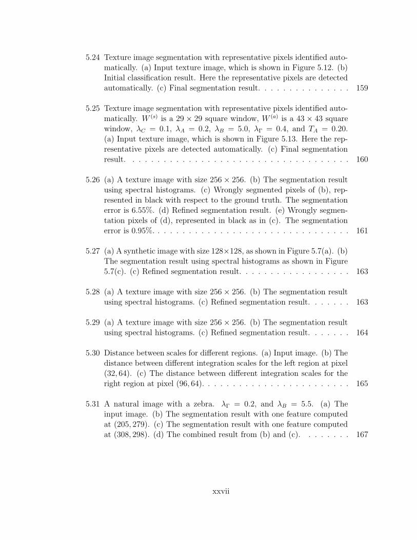
5.24 Texture image segmentation with representative pixels identified auto-matically. (a) Input texture image, which is shown in Figure 5.12. (b)Initial classification result. Here the representative pixels are detectedautomatically. (c) Final segmentation result. . . . . . . . . . . . . . . 159
5.25 Texture image segmentation with representative pixels identified auto-matically. W (s) is a 29 × 29 square window, W (a) is a 43 × 43 squarewindow, λC = 0.1, λA = 0.2, λB = 5.0, λΓ = 0.4, and TA = 0.20.(a) Input texture image, which is shown in Figure 5.13. Here the rep-resentative pixels are detected automatically. (c) Final segmentationresult. . . . . . . . . . . . . . . . . . . . . . . . . . . . . . . . . . . . 160
5.26 (a) A texture image with size 256× 256. (b) The segmentation resultusing spectral histograms. (c) Wrongly segmented pixels of (b), rep-resented in black with respect to the ground truth. The segmentationerror is 6.55%. (d) Refined segmentation result. (e) Wrongly segmen-tation pixels of (d), represented in black as in (c). The segmentationerror is 0.95%. . . . . . . . . . . . . . . . . . . . . . . . . . . . . . . . 161
5.27 (a) A synthetic image with size 128×128, as shown in Figure 5.7(a). (b)The segmentation result using spectral histograms as shown in Figure5.7(c). (c) Refined segmentation result. . . . . . . . . . . . . . . . . . 163
5.28 (a) A texture image with size 256× 256. (b) The segmentation resultusing spectral histograms. (c) Refined segmentation result. . . . . . . 163
5.29 (a) A texture image with size 256× 256. (b) The segmentation resultusing spectral histograms. (c) Refined segmentation result. . . . . . . 164
5.30 Distance between scales for different regions. (a) Input image. (b) Thedistance between different integration scales for the left region at pixel(32, 64). (c) The distance between different integration scales for theright region at pixel (96, 64). . . . . . . . . . . . . . . . . . . . . . . . 165
5.31 A natural image with a zebra. λΓ = 0.2, and λB = 5.5. (a) Theinput image. (b) The segmentation result with one feature computedat (205, 279). (c) The segmentation result with one feature computedat (308, 298). (d) The combined result from (b) and (c). . . . . . . . 167
xxvii

6.1 On- and off-center cell responses. (a) Input image. (b) On-center cellresponses. (c) Off-center cell responses (d) Binarized on- and off-centercell responses. White regions represent on-center response regions andblack off-center regions. . . . . . . . . . . . . . . . . . . . . . . . . . . 173
6.2 The figure-ground segregation network architecture for Figure 6.1(a).Nodes 1, 2, 3 and 4 belong to the white region; Nodes 5, 6, 7, and 8belong to the black region; Nodes 9 and 10, 11 and 12 belong to theleft and right gray regions respectively. Solid lines represent excitatorycoupling while dashed lines represent inhibitory connections. . . . . . 174
6.3 Temporal behavior of each node in the network shown in Figure 6.2.Each plot shows the status of the node with respect to the time. Thedashed line is 0.5. . . . . . . . . . . . . . . . . . . . . . . . . . . . . . 178
6.4 Surface completion results for Figure 6.1(a). (a) White region. (b)Gray region. (c) Black region. . . . . . . . . . . . . . . . . . . . . . . 180
6.5 Layered representation of surface completion for results shown in Fig-ure 6.4. . . . . . . . . . . . . . . . . . . . . . . . . . . . . . . . . . . . 180
6.6 Images with virtual contours. (a) Kanizsa triangle. (b) Woven square.(c) Double kanizsa. . . . . . . . . . . . . . . . . . . . . . . . . . . . . 181
6.7 Surface completion results for the corresponding image in Figure 6.6. 182
6.8 Images with virtual contours. (a) Kanizsa triangle. (b) Four crosses.(c) Overlapping rectangular bars. . . . . . . . . . . . . . . . . . . . . 183
6.9 Surface completion results for the corresponding image in Figure 6.8. 183
6.10 Images with virtual contours. (a) Original pacman image. (b) Mixedpacman image. (c) Alternate pacman image. . . . . . . . . . . . . . . 183
6.11 Layered representation of surface completion for the corresponding im-ages shown in Figure 6.10. . . . . . . . . . . . . . . . . . . . . . . . . 184
6.12 Bregman and real images. (a) and (b) Examples by Bregman [9]. (c)A grocery store image. . . . . . . . . . . . . . . . . . . . . . . . . . . 185
6.13 Surface completion results for images shown in Figure 6.12. . . . . . . 185
xxviii
6.14 Bistable perception. (a) Face-vase input image. (b) Faces as figures.(c) Vase as figure. . . . . . . . . . . . . . . . . . . . . . . . . . . . . . 186
6.15 Temporal behavior of the system for Figure 6.14(a). Dotted lines are0.5. . . . . . . . . . . . . . . . . . . . . . . . . . . . . . . . . . . . . . 187
7.1 Classification result of a noisy synthetic image using a three-layer per-ceptron. (a) The input image with size of 230 × 240. (b) The groundtruth image. (c) Positive and negative training samples. Positive ex-amples are shown as white and negative ones as black. (d) Classifica-tion result from a three-layer perceptron. . . . . . . . . . . . . . . . . 190
7.2 Lateral connection evolution through weight adaptation illustrated us-ing the 170th row from the image shown in Figure 7.1(a). (a) Theoriginal signal. (b) Initial connection weights. (c) Connection weightsafter 40 iterations. (d) Corresponding smoothed signal. . . . . . . . . 194
7.3 Architecture and local features for the seed selection neural network. 202
7.4 Segmentation result using the proposed method for a synthetic image.(a) A synthetic image as shown in Figure 7.1(a). (b) The segmentationresult from the proposed method. Here Wz = 0.25 and θp = 100. . . . 204
7.5 A DOQQ image with size of 6204×7676 pixels of the Washington East,D.C.-Maryland area. . . . . . . . . . . . . . . . . . . . . . . . . . . . 207
7.6 Seed pixels obtained by applying a trained three-layer perceptron tothe DOQQ image shown in Figure 7.5. Seed pixels are marked as whiteand superimposed on the original image. The network is trained using19 positive and 28 negative samples, where each sample is a 31 × 31window. . . . . . . . . . . . . . . . . . . . . . . . . . . . . . . . . . . 208
7.7 Extracted hydrographic regions from the DOQQ image shown in Figure7.5. Hydrographic regions are marked as white and superimposed onthe original image to show the accuracy of the extracted result. HereWz = 0.15 and θp = 4000. . . . . . . . . . . . . . . . . . . . . . . . . 209
7.8 A ground truth generated by manually placing seeds based on the cor-responding 1:24,000 USGS topographic map and DOQQ image. Theresult was manually edited. . . . . . . . . . . . . . . . . . . . . . . . 210
xxix

7.9 Hydrographic region extraction result for an aquatic garden area withmanually placed seed pixels. Due that no reliable seed region is de-tected, this aquatic region, which is very similar to soil regions, is notextracted from the DOQQ image as shown in Figure 7.7. Extractedregions are marked as white and superimposed on the original image. 211
7.10 Extraction result for an image patch from Figure 7.5. (a) The inputimage. (b) The seed points from the neural network. (c) A topographicmap of the area. Here the map is scanned from the chapter versionand not wrapped with respect to the image. (d) Extracted result fromthe proposed method. Extracted regions are represented by white andsuperimposed on the original image. . . . . . . . . . . . . . . . . . . . 213
7.11 A DOQQ image with size of 5802 × 7560 pixels of Damascus,Pennsylvania-New York area. . . . . . . . . . . . . . . . . . . . . . . 215
7.12 Extracted hydrographic regions from the DOQQ image shown in Fig-ure 7.11. The extracted regions are represented by white pixels andsuperimposed on the original image. . . . . . . . . . . . . . . . . . . . 216
7.13 A ground truth generated based on a 1:24,000 USGS topographic mapand DOQQ image. . . . . . . . . . . . . . . . . . . . . . . . . . . . . 217
8.1 A stereo image pair and correspondence using the spectral histogram.(a) The left image. (b) The right image. (c)-(e) The matching resultsof marked pixels in the left image. In each row, the left shows themarked pixel, the middle shows the probability of being a match inthe paired image, and the right shows the high probability area in thepaired image. . . . . . . . . . . . . . . . . . . . . . . . . . . . . . . . 224
8.2 Comparison between en edge detector and the spectral histogram usinga natural image of a giraffe. (a) The input image with size 300 ×240. (b) The edge map from a Canny edge detector [13]. (c) Theinitial classification result using the method presented in Chapter 5. Aspectral histogram is extracted at pixel (209, 291) and the segmentationscale is 29× 29. (d) The initial classification is embedded in the inputimage to show the boundaries. . . . . . . . . . . . . . . . . . . . . . . 226
xxx

CHAPTER 1
INTRODUCTION
1.1 Motivations
“Vision is the process of discovering from images what is present in the world and
where it is” (Marr [88], p. 3). Due to the apparent simplicity of the action of seeing,
however, the underlying difficulties of visual information processing had not been
realized until Marr’s pioneer work on computational vision. According to Marr, the
ultimate task of any computer vision system is essentially to “transform” an array of
input numerical values into meaningful description that a human normally perceives.
Figure 1.1(a) shows an image which consists of two texture regions. However, the
texture regions are not obvious at all from the numerical values, where a small portion
is shown in Figure 1.1(c).
While the true “transformation” employed by humans is not known, any algorithm
for solving vision problems attempts to approximate the transformation based on
different assumptions and constraints with respect to the problems to be solved.
Existing approaches can thus be categorized according to the problems to be solved
and their assumptions. Due to the complexities of the vision process, four problems
are widely studied in computer vision relatively independently: edge detection, stereo
1
(a) (b)
67 6d 68 65 6a 73 6c 6a 69 75 77 76 74 78 78 7f 7b 7c 7d 7e 87 7b 86 bd a6 85 8e b4 8d 95 8c 82 89 83 8a 84 89 81 94 91 8d
69 6b 63 6f 6c 69 6b 6c 70 6e 6c 6b 74 71 75 71 73 6d 93 8b 7e 7f 81 b7 8f 93 51 c9 a9 c0 80 81 7d 80 7e 8e 7e 8d 85 87 8d
6b 71 6c 6e 6b 6e 67 67 66 67 bb ee ac 81 b8 b6 9c 57 7a 8c 5d 72 84 d0 8b ab b2 8d d0 bd 8f 84 7a 86 7c 85 87 8e 86 92 94
6a 6c 62 6d 6a 6d 6e 73 6c 69 b8 9e a6 6b 4e a5 87 94 51 a7 79 7e 59 ad 80 7e 7a 70 b9 7b 91 85 7d 87 81 89 86 8e 88 91 91
63 5d 69 75 68 6a 64 67 b0 e5 ce 5c 8e 7d 64 6c 98 bd 88 9a 96 92 7e 3d 9b 8c 92 97 87 94 cc 7d 85 7c 87 8d 91 83 87 96 95
6b 65 6a 6e 67 6c 78 94 dd 9e e4 65 84 85 5e 6b 87 b9 a4 ae 9b 9f 98 83 8b 92 5f a6 7f a8 ab 7c 81 84 87 87 8b 8a 8f 8d 93
69 69 72 73 6c 77 66 61 a8 a7 a9 a2 5f a5 63 92 8c a8 a0 97 9c a2 96 56 9d 9d 8a 9f a7 ac b0 81 80 83 87 89 89 8e 93 8b a0
73 6c 70 6b 78 70 70 61 ef e7 d1 a5 82 8e c5 40 7f 9f 9f a2 a3 a6 a0 9d 9e 8f 74 84 9a ca c7 86 80 85 89 86 87 8e 98 90 96
6e 72 6c 6c 6d 75 68 71 dd e0 c6 c4 c2 b0 b6 8e 90 88 9f 9a 9f a3 99 a0 9d a1 70 8a 95 eb b9 7b 84 8a 82 8a 86 89 91 9b 95
68 6c 77 6e 6d 73 72 fb d0 da 9f 8f be c0 a8 aa a0 9f 93 95 a1 a4 9d 9e a8 81 78 7d 9e ce 8e 81 85 8c 83 88 8d 9a 8f 96 9a
71 6f 77 73 72 68 71 e3 e0 dd da c0 a4 d7 a1 a1 85 95 8f 98 a0 af a5 9e a7 8b 4d 9c 86 a7 a6 81 87 85 87 8e 8e 95 93 95 9d
6d 74 72 73 6c 78 67 e6 cf d8 c8 da ad a1 ca b1 fb a4 5f 92 a2 b4 b5 a3 9b 7f 82 b2 4f dd dd ff 88 8d 84 82 90 8e 92 91 97
65 72 70 6f 69 71 6d f5 af e3 d0 c0 c2 b7 a7 b2 a2 a6 7f 79 c8 a5 a2 a6 a3 9a 88 71 59 b6 d9 99 8a 8a 87 89 90 8e 9a 97 9a
71 6e 6b 6f 71 67 78 fc f5 e0 b1 a3 cc a2 d0 a0 ae a0 93 8f ab be a5 a9 a1 a2 87 7e 8a b1 8f 87 86 8a 8d 8c 93 97 94 92 99
72 6d 6c 79 6f 6d 73 df d4 e2 9b 84 c0 b0 9d a0 ce 9b ac bb 9b ac aa 9a a9 90 86 74 94 c6 83 85 88 8c 88 8c 91 90 91 95 99
6f 78 6d 6f 70 73 6c cf f3 ce bb a2 c0 94 c9 bf 94 9a 9d a0 ad ad b3 a6 ad a3 86 7f b7 92 7a 89 91 8c 8f 8c 91 92 8e 99 9a
71 63 70 67 72 71 78 ec bd cb c5 d8 94 a7 a0 b6 90 74 c8 a7 ab a8 aa bb af bc 8d 94 6e dc 8c 8d 88 8f 8c 91 92 93 90 95 9a
6d 6d 6c 74 68 69 6c ff d9 df fa d2 b8 ad 8b b1 b7 cd c8 ad a8 b6 af b4 bd 88 84 7d 8a b4 8a 8b 8f 8c 96 91 91 9d 94 9b 99
6e 6c 70 74 74 6c 6e ff f4 f0 d8 c5 db 8f a1 b1 c3 f6 d5 95 a8 b5 aa b1 e9 e4 78 7d 8c 87 91 87 93 8f 93 8e 90 96 91 96 9c
6e 73 6a 71 6f 72 5e dd f4 ef d5 ba bb aa ab aa ae ae ae 96 ab c1 f9 90 c2 f3 ed c4 81 7f 89 86 8d 86 8a 89 93 96 93 97 9c
73 76 73 6e 6d 6c ff da e6 dc cc b4 ae b5 ae 9e d5 ae ba af 93 a4 b5 ea b1 d3 e7 ff e9 81 87 89 89 8b 8b 8f 8b 90 92 94 a0
72 70 6a 73 74 6f f7 c1 97 d8 c4 bb ab ac a7 af a3 aa b1 c5 e8 c3 af 94 9e b2 d6 cd ee de 85 81 89 84 87 90 94 9f 94 94 97
6b 68 71 74 70 6d 63 5d e5 d8 cb bb b8 ae aa a9 a3 9b a9 ca e3 ff b5 b6 8f 9b af aa b6 eb c1 80 7e 87 8d 8b 91 95 94 95 97
74 70 6d 72 73 70 60 63 cc d7 c0 b3 bf b6 b3 ad a6 92 a3 c8 de ff a7 bd b5 9b 9c 98 9b d0 a6 e5 83 84 88 8a 8a 91 97 99 9e
6c 6e 6e 76 6c 6f 67 68 ff e9 c5 b9 b4 b3 c8 c8 b0 98 a9 b9 d2 ff 82 80 84 87 92 94 98 af aa d1 d9 7b 80 85 8e 87 8e 96 98
69 70 67 70 72 6e 6d 63 5f e1 c9 ba ba b3 f6 cd c2 b4 a4 b9 d3 e8 ff 7e 7e 7b 8a 8d 96 7f 9b b3 d3 d7 6e 86 82 8b 8d 8e 96
6c 64 69 6a 71 6b 76 6c 61 db bd b6 a6 ee d9 d4 c4 b5 ad ac c7 d9 ea 81 79 82 86 8a b5 8b a5 a8 ad c0 dc 76 80 80 8d 91 93
68 64 67 5d 71 65 63 65 5c c3 a9 a9 99 de e5 d5 bd ae a5 ab bb c8 d7 e3 80 7a 7a d2 b9 94 89 92 9f a0 ad d9 7b 7b 7f 87 92
63 6d 6a 5b 58 5e 5c 59 5a 63 8f 9c 76 db de c0 bd b9 b0 a9 b1 c2 bd c9 d4 7a 81 76 6f 83 87 84 8e 95 95 c2 ee 7a 7f 88 87
67 64 59 66 60 66 62 5f 5f 5b 69 63 5f e9 cf b5 b0 ae ae b6 b0 bd c6 bb c9 cb 86 79 85 8a 87 8e 83 89 8e ad d5 e3 7d 79 85
63 68 69 62 67 63 59 67 67 68 5a 5e d6 bd ba b3 aa af ad b4 b7 bd c3 b9 bf c5 d3 cc 75 8f 9a 95 97 91 8c 9d a9 dc f3 83 89
5a 63 59 69 64 63 5d 5c 68 5d 8d d0 b9 ab a9 a7 ac af b5 c2 c3 bd b2 af b5 c2 c0 d2 d4 b7 b9 97 9a 94 91 89 8f ae ff a8 71
61 67 5f 65 5c 5f 59 4f 6d c5 bd ae ab a0 a9 a3 b1 b7 b9 c2 c8 c0 a9 9c a5 ba c6 d4 dc da c1 c6 c8 8a 83 84 91 b3 c7 ff 7d
68 61 5c 5c 5a cb be bb b8 ba aa a8 a2 92 9c 9a a1 bc ba c5 d5 b9 a0 93 a4 b6 c5 de ee ee de c1 cc d9 b2 b7 ac b2 c3 da bd
5f 5c 54 d0 bd b5 b1 ad a7 9f a3 9a 94 9b 8c 98 a5 b6 c7 d2 e6 c7 9c 8b 94 b4 c2 e2 fe f0 e5 dc e7 de df b4 c1 cc d4 f6 f4
55 74 d0 c1 b8 b2 a6 a4 9e 9b 9d 97 8e 8e 91 95 ac b5 cc e4 ef c8 9e 8c 91 b1 c5 ef ff fd f1 e7 ee f1 dd d4 cf cc dc e5 e2
82 ca c4 ba ab a6 9e 9f 9b 99 9a 8e 88 90 99 98 a1 b4 cc ea ff c8 97 86 97 ae c0 f5 ff f4 f6 e9 e6 e2 df d3 d9 dd e3 ea d5
d0 c3 b3 a6 b1 a2 a4 9b 94 8f 92 88 80 8f 95 95 9e b5 cf ee fb ce 98 8c 90 a7 c4 e9 ff f4 eb e4 d9 d0 d8 d1 d7 e2 d6 e6 d9
ce bd b7 ac a7 a0 a3 9a 92 8e 83 90 8a 91 94 9b 9d ba d7 f2 ff d4 9a 87 96 a7 c6 e3 f9 f9 f9 e4 d9 d7 de de ec ee ea f3 e4
(c)
Figure 1.1: A texture image and the corresponding numerical arrays. (a) A textureimage with size 128×64. (b) A small portion with size 40×30 of (a) centered at pixel(64, 37), which is on the boundary between the two texture regions. (c) Numericalvalues of (b). To save space, the values are displayed in hexadecimal format.
2
matching and motion analysis, image segmentation and perceptual organization, and
pattern recognition. Roughly speaking, the techniques for the first three problems
are primarily data-driven, or called bottom-up processes, and pattern recognition is
model-driven, or called top-down process.
Early techniques with successful applications are classification techniques [25],
which map a given input into one of the pre-defined classes according to a distance
measure. However, all the possible classes and their variations we normally perceive
are too gigantic to be implemented effectively in any system. The attention of com-
puter vision was then shifted to derive more generic features for arbitrary images.
From information and encoding theories, edges, i.e., discontinuities in images, carry
more information and exhibit nice properties such as invariance to luminance changes.
Motivated by neurophysiological findings [53], many edge detection algorithms were
proposed and studied. Segmentation techniques try to solve the same problem by
segmenting an image into homogeneous regions, where edges and region contours can
be obtained straightforwardly and more robustly. These approaches were claimed to
be unified [92] through what is called Mumford-Shah Segmentation energy functional
[94] (See Chapters 4 and 5). Common to these approaches, the images are assumed
to be piece-wise smooth regions with additive Gaussian noise, resulting in efficient
algorithms. To improve the performance for real images, multiple scales are generally
needed and linear and nonlinear scale spaces are thus proposed and studied. Chapter
2 studies segmentation for range images. Chapter 3 studies a new nonlinear smooth-
ing algorithm and addresses some of problems in nonlinear scale spaces. Chapter
7 applies a nonlinear smoothing algorithm to hydrographic object extraction from
remotely sensed images.
3
While there are useful applications of edge detection and segmentation algorithms,
the underlying assumption limits their successes in dealing with natural images. As
shown in Figure 1.1, texture regions neither are piece-wise smooth nor can be modeled
with additive Gaussian noise. Figure 1.2 demonstrated that a pure linear system is
not sufficient for natural image modeling [63], where the spatial relationships among
pixels are more prominent in characterizing the texture regions than individual pixels.
Clearly piece-wise smooth regions with additive Gaussian noise are not sufficient and
more sophisticated models are needed to deal with texture images.
Supported by neurophysiological and psychophysical experiments [12] [23], The
early processes in the human vision system can be abstractly modeled by filtering
with a set of frequency and orientation tuned filters. However, as demonstrated in
Figure 1.2, purely linear filtering is not sufficient, nonlinearity beyond filtering must
be incorporated [87]. Spectral histograms integrate the responses of a chosen bank
of filters through marginal distributions [148] [149] [150] [147]. As demonstrated
in Figure 1.2, spectral histograms are nonlinear. Chapters 4 and 5 apply spectral
histograms to modeling [147], classification, and segmentation of texture as well as
intensity images.
While edge detection and segmentation techniques are very fruitful, there are
perceptual phenomena that cannot be explained by purely data-driven processes.
Classical examples include virtual contours, which are widely studied by Gestaltists.
The long-range order grouping is known as perceptual organization. Chapter 6 studies
perceptual organization through temporal dynamics.
Because many of the meaningful objects cannot be characterized well using in-
tensity values or even textures, such as a human face, the relationships among some
4
(a) (b)
(c)
Figure 1.2: Demonstration of nonlinearity for texture images. (a) A regular textureimage. (b) The image in (a) was circularly shifted left and downward for 2 pixels ateach direction. (c) The pixel-by-pixel average of (a) and (b). The relative variancedefined in (3.20) between (a) and (b) is 137, and between (a) and (c) is 69. Thedistance between the spectral histograms defined in Chapter 4 between (a) and (b)is 1.288 and between (a) and (c) is 38.5762.
5
primitives need to be modeled. This leads to the need of top-down processes such as
recognition. Clearly, the four problems studied are sub-problems of vision process and
the integration among them is critical for a complete vision system. The interaction
between different modules is briefly discussed in Chapter 8.
1.2 Thesis Overview
As discussed above, we study vision problems at different organizational levels
in this dissertation. In Chapter 2, we study the segmentation problem for range
images. Depth is most important cue for visual perception and range image segmen-
tation has a wide range of applications. We propose a feature vector consisting of
surface normal, mean and Gaussian curvatures and a similarity measure for range
images. We implemented a system based on oscillatory correlation using a LEGION
(locally excitatory globally inhibitory oscillator network) network. Experimental re-
sults demonstrate that our system is capable of handling different kinds of surfaces.
With the unique properties of a temporal dynamic system, our approach may lead to
a real-time approach for range image segmentation.
In Chapter 3, we propose a new nonlinear smoothing algorithm by incorporating
contextual information and geometrical constraints. Several nonlinear algorithms are
derived as special cases of the proposed one. We have compared the temporal behavior
and boundary detection results of several widely algorithms, including the proposed
method. The proposed algorithm gives quantitatively good results and exhibits nice
temporal behaviors such as quick convergence and robustness to noise.
In Chapter 4, we propose spectral histograms as a generic statistic feature for tex-
ture as well as intensity images. We demonstrate the properties of spectral histograms
6
using image synthesis, image classification, and content-based image retrieval. We
also compare with several widely used statistic features for textures and show that
the distribution of local features is critically important for classification while mean
and variance in general are not sufficient. We also propose a model for texture dis-
crimination, which matches the existing psychophysical data well.
Chapter 5 continues the work in Chapter 4. In Chapter 5, segmentation prob-
lem is studied extensively using spectral histograms. A new energy functional for
segmentation is proposed by making explicit the homogeneity measures. An approx-
imate algorithm is derived, implemented and studied under different assumptions.
Satisfactory results have been obtained using natural texture images.
Chapter 6 studies the problem of perceptual organization and long-range grouping,
which is one level beyond the segmentation. By using a boundary-pair representa-
tion, we propose a figure-ground segregation network. Gestalt-like grouping rules are
incorporated by modulating the connection weights in the network. The network can
explain many perceptual phenomena such as modal and amodal completion, shape
composition and perceptual grouping using a fixed set of parameters.
Chapter 7 presents a computational framework for feature extraction from remote
sensing images for map revision and geographic information extraction purposes. A
multi-layer perceptron is used to learn the features to be extracted from examples. A
locally coupled LEGION network is used to achieve accurate boundary localization.
To increase the robustness of the system, a weight adaption method is used. Ex-
perimental results using DOQQ images show that our system can handle very large
images efficiently and may have a wide range of applications.
7

Chapter 8 summarizes the contributions of the work presented in this dissertation
and concludes this dissertation with discussions on the future work.
8
CHAPTER 2
RANGE IMAGE SEGMENTATION USING A
RELAXATION OSCILLATOR NETWORK
In this chapter, a locally excitatory globally inhibitory oscillator network (LE-
GION) is constructed and applied to range image segmentation, where each oscillator
has excitatory lateral connections to the oscillators in its local neighborhood as well
as a connection with a global inhibitor. A feature vector, consisting of depth, surface
normal, and mean and Gaussian curvatures, is associated with each oscillator and is
estimated from local windows at its corresponding pixel location. A context-sensitive
method is applied in order to obtain more reliable and accurate estimations. The lat-
eral connection between two oscillators is established based on a similarity measure
of their feature vectors. The emergent behavior of the LEGION network gives rise to
segmentation. Due to the flexible representation through phases, our method needs
no assumption about the underlying structures in image data and no prior knowledge
regarding the number of regions. More importantly, the network is guaranteed to con-
verge rapidly under general conditions. These unique properties lead to a real-time
approach for range image segmentation in machine perception. The results presented
in this chapter appeared in [83].
9
2.1 Introduction
Image segmentation has long been considered in machine vision as one of the fun-
damental tasks. Range image segmentation is especially important because depth
is one of the most widely used cues in visual perception. Due to its practical
importance, many techniques have been proposed for range image segmentation,
and they can be roughly classified into four categories: 1) edge-based algorithms
[91][6][136]; 2) region-based algorithms [129][4][71][58][51]; 3) classification-based ap-
proaches [56][49][67][51][5];
4) global optimization of a function [73].
Edge-based algorithms first identify the edge points that signify surface discon-
tinuity using certain edge detectors, and then try to link the extracted edge points
together to form surface boundaries. For example, Wani and Batchelor [136] intro-
duced specialized edge masks for different types of discontinuity. Because critical
points, such as junctions and corners, could be degraded greatly by edge detectors,
they are extracted in an additional stage. Then surface boundaries are formed by
growing from the critical points. As we can see, many application-specific heuris-
tics must be incorporated in order to design good edge detectors and overcome the
ambiguities inherent in linking.
Region-based algorithms were essentially similar to region-growing and split-and-
merge techniques for intensity images [152], but with more complicated criteria to
incorporate surface normal and curvatures which are critical for range image segmen-
tation. A commonly used method is iterative surface fitting [4][71][51]. Pixels are first
coarsely classified based on the sign of mean and Gaussian surface curvature and seed
regions are formed based on initial classification. Neighboring pixels will be merged
10

into an existing surface region if they fit into the surface model well. This procedure
is done iteratively. As pointed by Hoffman and Jain [49], the major disadvantage is
that many parameters need to be involved. Also a good surface model that fits the
range image data must be provided in order to obtain good results.
In classification-based approaches, range image segmentation is posed as a vector
quantization problem. Each pixel is associated with an appropriate feature vector.
The center vector for each class can be obtained by applying some clustering algo-
rithms which minimize a certain error criterion [49] or alternatively by training [67][5].
Then each pixel is associated with the closest cluster center. The segmentation re-
sult from the classification can be further refined by a merging procedure similar
to region-growing [49][67][51][5]. One of the limitations of classification-based ap-
proaches is that the number of regions must be given a priori, which, generally, is not
available. Koh et al. [67] and Bhandarkar et al. [5] tried to address this issue by using
a hierarchical self-organizing network for range image segmentation. At each level, a
self-organizing feature map (SOFM) [68] is used to segment range images into a given
number of regions. An abstract tree [67] is constructed to represent the output of the
hierarchical SOFM network. The final segmentation is obtained by searching through
the abstract tree, which is sequential and similar to a split-and-merge method. Thus
the solution suffers from the disadvantages of region-based algorithms. In addition,
the problem of prior specification of number of regions is not entirely solved because
the number of regions for each level still needs to be specified.
A more fundamental limitation common to all region- and classification-based ap-
proaches is that the representation is too rigid, i.e., different regions are represented
through explicit labels, which forces the approaches to be sequential to a large extent.
11
Energy minimization techniques [35] can be inherently parallel and distributed and
have been widely used in image classification and segmentation. In this framework,
solutions are found by minimizing energy functions using relaxation algorithms1. Li
[73] constructed a set of energy functions for range image segmentation and recogni-
tion by incorporating surface discontinuity through mean and Gaussian curvatures.
Minimization algorithms were obtained based on regularization techniques [124] and
relaxation labeling algorithms [112][55]. While the approach was quite successful, the
main problem is that the algorithms are too computationally expensive for real-time
applications [88][36].
In this chapter, we use a novel neural network for segmenting range images, which
overcomes some of the above limitations. Locally excitatory globally inhibitory oscil-
lator network (LEGION) [123][134][135] provides a biologically plausible framework
for image segmentation in general. Each oscillator in the LEGION network connects
excitatorily with the oscillators in its neighborhood as well as inhibitorily with a
global inhibitor. For range image segmentation, the feature detector associated with
each oscillator estimates the surface normal and curvatures at its corresponding pixel
location. The lateral connection between two oscillators is set at the beginning based
on a similarity measure between their feature vectors. The segmentation process is
the emergent behavior of the oscillator network. Because the results are encoded flex-
ibly through oscillator phases, segmentation is inherently parallel and no assumption
about the underlying structures in image data is needed.
1“Relaxation” used in relaxation labeling technique [112] refers to an optimization technique thatglobal optimal solutions can be obtained by satisfying local constraints. This is very different fromthe term “relaxation” as used in relaxation oscillators, where it refers to the change of activity on aslow time scale (see Section 2.2).
12

The rest of this chapter is organized as follows. Section 2.2 gives an overview of the
LEGION network. Section 2.3 presents feature vector estimation for range images.
Section 2.4 provides experimental results and comparisons with other approaches.
Section 2.5 justifies the biological plausibility of this approach and gives a comparison
with pulse-coupled neural networks (PCNN). This chapter appeared in [83].
2.2 Overview of the LEGION Dynamics
A fundamental problem in image segmentation is to group similar input elements
together while segregating different groups. Temporal correlation was hypothesized as
a representational framework for brain functions [90][130], which has received direct
supports from neurophysiological findings of stimulus-dependent oscillatory activities
in the visual cortex [26][40]. The LEGION network [123][134], which is based on
oscillatory correlation, was proposed as a computational model to address problems
of image segmentation and figure-ground segregation [135]. In this section, after
briefly introducing the single oscillator model, we summarize the properties of the
network and demonstrate the network’s capability using a synthetic image.
2.2.1 Single Oscillator Model
As the building block of LEGION, a single oscillator i is defined as a feedback loop
between an excitatory unit ui and an inhibitory unit vi [135] with one modification:
dui
dt= 3ui − u3
i + 2− vi + IiH(pi − θ) + Si + ρ (2.1a)
dvi
dt= ε(γ(1 + tanh(ui/β))− vi) (2.1b)
13

Here H stands for the Heaviside step function. Ii represents external stimula-
tion for the oscillator i, which is assumed to be applied at time 0. ρ denotes a
Gaussian noise term to test the robustness of the system and play an active role in
desynchronization. Si denotes the coupling from other oscillators in the network, and
pi the potential of the oscillator i. θ is a threshold, where 0 < θ < 1. The only
difference between the definition in [135] and the one given here is that the term
H(pi + exp(−at)− θ) in [135] is replaced by H(pi− θ) in (2.1a) so that the Heaviside
term in (2.1) does not depend explicitly on time.
The parameter ε is a small positive number. In this case, equation (2.1), without
any coupling or noise but with constant stimulation, corresponds to a standard relax-
ation oscillator, similar to the van der Pol oscillator [128]. The u-nullcline (du/dt = 0)
of (2.1) is a cubic curve, and the v-nullcline (dv/dt = 0) is a sigmoid function, the
steepness of which is specified by β. If I > 0 and H = 1, which corresponds to a
positive stimulation, (2.1) produces a stable periodic orbit for all sufficiently small
values of ε, alternating between left and right branches of near steady-state behavior.
Figure 2.1 shows a stable limit cycle along with nullclines. The oscillator travels on
left and right branches on a slow time scale because the driving force is mainly from
the inhibitory unit and is weak, while the transition between two branches occurs
on a fast time scale because the driving force is mainly from the excitatory unit and
is strong. The slow and fast time scales result from a small ε and produce highly
nonlinear activities.
The parameter γ is used to control the ratio of the times that an oscillator spends
on the right and left branches. Figure 2.2 shows the temporal activities of the excita-
tory unit for γ = 3 and γ = 40. If γ is chosen to be large, the output will be closer to
14
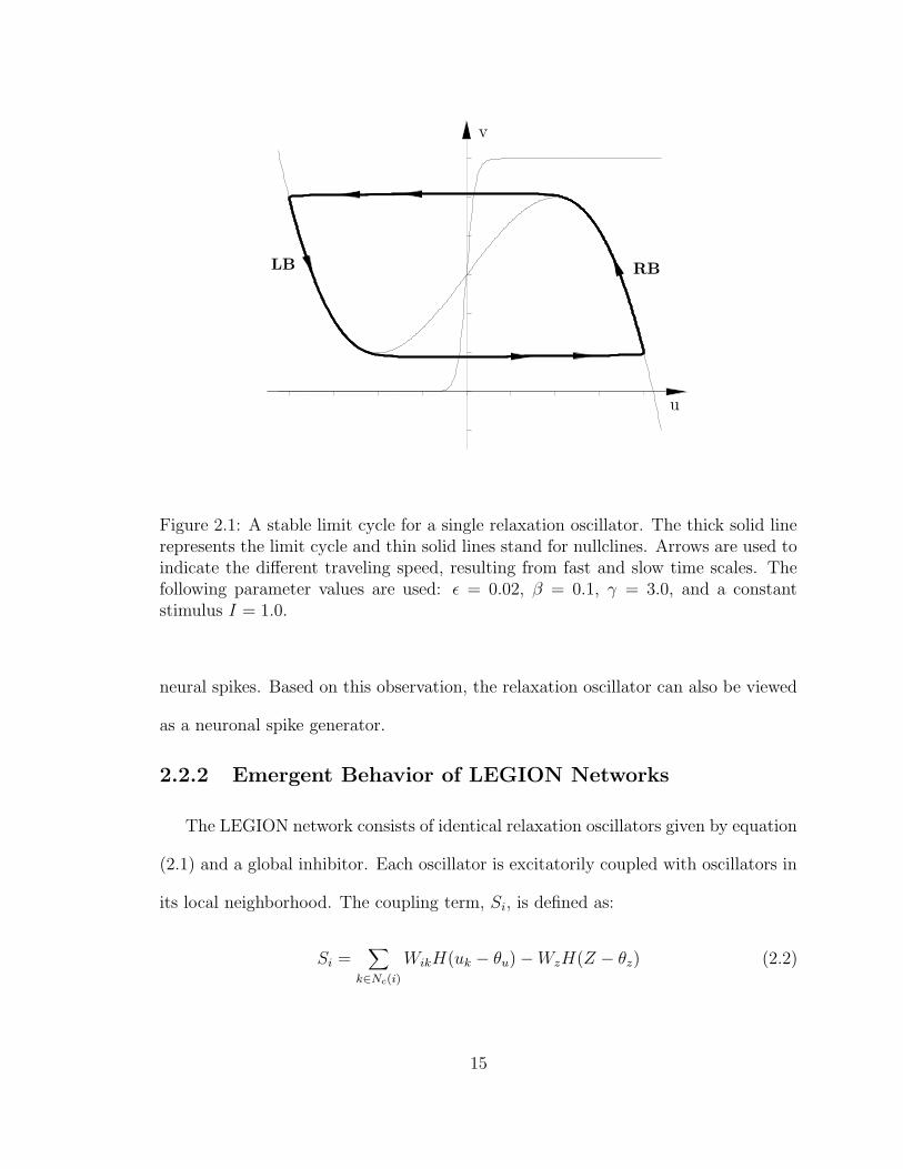
u
v
LB RB
Figure 2.1: A stable limit cycle for a single relaxation oscillator. The thick solid linerepresents the limit cycle and thin solid lines stand for nullclines. Arrows are used toindicate the different traveling speed, resulting from fast and slow time scales. Thefollowing parameter values are used: ε = 0.02, β = 0.1, γ = 3.0, and a constantstimulus I = 1.0.
neural spikes. Based on this observation, the relaxation oscillator can also be viewed
as a neuronal spike generator.
2.2.2 Emergent Behavior of LEGION Networks
The LEGION network consists of identical relaxation oscillators given by equation
(2.1) and a global inhibitor. Each oscillator is excitatorily coupled with oscillators in
its local neighborhood. The coupling term, Si, is defined as:
Si =∑
k∈Nc(i)
WikH(uk − θu)−WzH(Z − θz) (2.2)
15

(a)
(b)
Figure 2.2: The temporal activities of the excitatory unit of a single oscillator fordifferent γ values. Other parameters are same as for Figure 2.1. (a) γ = 3.0. (b)γ = 40.0.
16
Here θu and θz are thresholds. Wik is the connection weight from oscillator k to
i, and Nc(i), the coupling neighborhood of i, is the set of neighboring oscillators of
i. An oscillator only sends excitation to its neighbors only when its activity is higher
than the threshold θu. In that case, we refer that it is in active phase. Otherwise, it
is in silent phase. This results in Heaviside coupling.
With excitatory coupling, the distance between two oscillators must decrease at
an exponential rate when traveling on the same branch. During jumps between
left and right branches, the time difference, the time that is needed to travel the
distance between them, will be compressed even though the Euclidean distance does
not change. These two factors lead to the fact that the two oscillators must get
synchronized at an exponential rate [123][134][135].
The global inhibitor Z leads to desynchronization among different oscillator groups
[123][134]. In (2.2), Wz is the weight of inhibition from the global inhibitor Z, which
is defined by:
dZ
dt= φ(σ∞ − Z) (2.3)
Where σ∞ = 1 if ui ≤ θz for at least one oscillator i, and σ∞ = 0 otherwise. Under
this condition, only an oscillator in the active phase can trigger the global inhibitor.
When one oscillator group is active, it suppresses the other groups from jumping
up by activating the global inhibition. Architecturally, the global inhibitor imposes
constraints on the entire network and effectively reduces the collisions from local
coupling. This is a main reason why LEGION networks are far more efficient than
purely locally coupled cooperative processes, including relaxation labeling techniques
[112][55][35], which tend to be very slow [88][36].
17
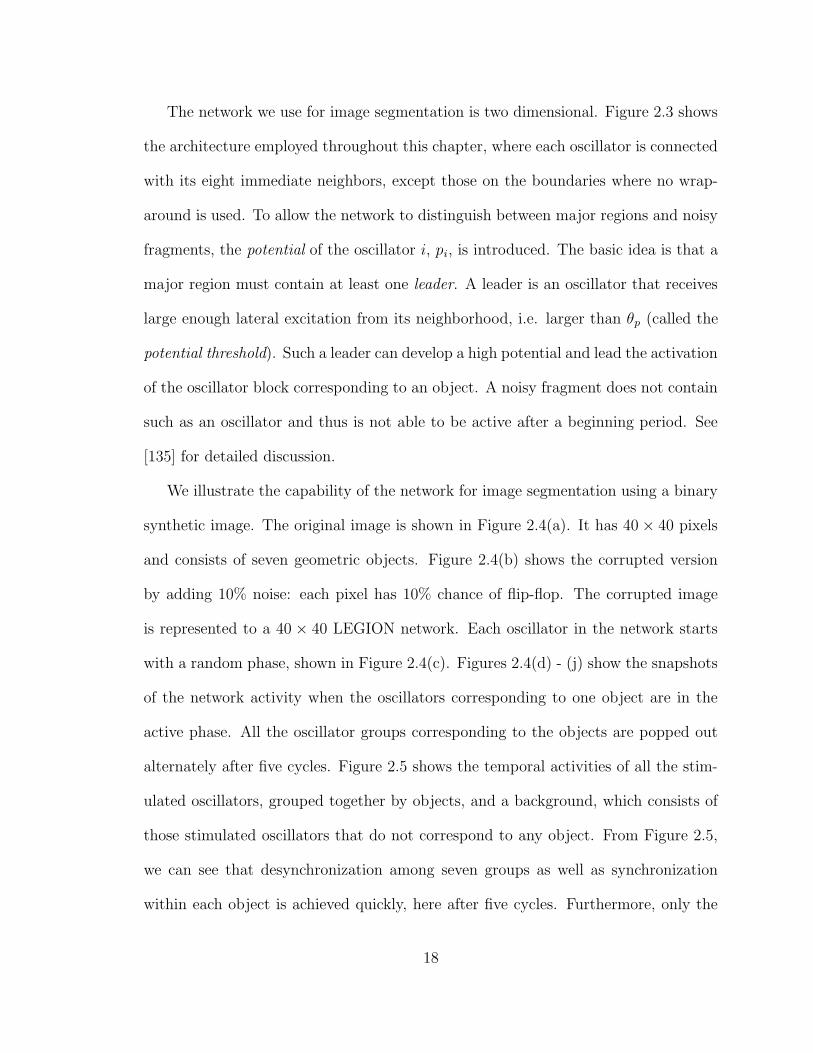
The network we use for image segmentation is two dimensional. Figure 2.3 shows
the architecture employed throughout this chapter, where each oscillator is connected
with its eight immediate neighbors, except those on the boundaries where no wrap-
around is used. To allow the network to distinguish between major regions and noisy
fragments, the potential of the oscillator i, pi, is introduced. The basic idea is that a
major region must contain at least one leader. A leader is an oscillator that receives
large enough lateral excitation from its neighborhood, i.e. larger than θp (called the
potential threshold). Such a leader can develop a high potential and lead the activation
of the oscillator block corresponding to an object. A noisy fragment does not contain
such as an oscillator and thus is not able to be active after a beginning period. See
[135] for detailed discussion.
We illustrate the capability of the network for image segmentation using a binary
synthetic image. The original image is shown in Figure 2.4(a). It has 40× 40 pixels
and consists of seven geometric objects. Figure 2.4(b) shows the corrupted version
by adding 10% noise: each pixel has 10% chance of flip-flop. The corrupted image
is represented to a 40 × 40 LEGION network. Each oscillator in the network starts
with a random phase, shown in Figure 2.4(c). Figures 2.4(d) - (j) show the snapshots
of the network activity when the oscillators corresponding to one object are in the
active phase. All the oscillator groups corresponding to the objects are popped out
alternately after five cycles. Figure 2.5 shows the temporal activities of all the stim-
ulated oscillators, grouped together by objects, and a background, which consists of
those stimulated oscillators that do not correspond to any object. From Figure 2.5,
we can see that desynchronization among seven groups as well as synchronization
within each object is achieved quickly, here after five cycles. Furthermore, only the
18
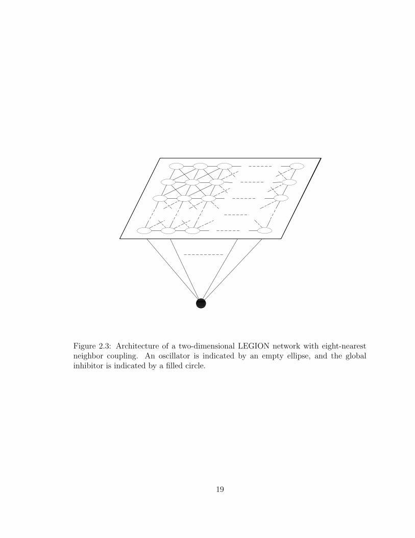
Figure 2.3: Architecture of a two-dimensional LEGION network with eight-nearestneighbor coupling. An oscillator is indicated by an empty ellipse, and the globalinhibitor is indicated by a filled circle.
19

oscillators belonging to an object can stay oscillating and all other noisy fragments
are suppressed into the background after two cycles.
Formally, it has been proved [123][135] that the LEGION network can achieve
synchronization among the oscillators corresponding to the same object and desyn-
chronization between groups corresponding to different objects quickly under general
conditions. In particular, synchronization within an object and desynchronization
among different objects can be achieved in NM + 1 cycles, where NM is the number
of the major regions corresponding to distinct objects.
2.3 Similarity Measure for Range Images
Given the LEGION dynamics, the main task is to establish lateral connections
based on some similarity measure. Intuitively, neighboring pixels belonging to the
same surface should be similar and thus should have strong connections with each
other in the LEGION network. To be effective for range image segmentation, we
consider different types of surfaces. For planar surfaces, surface normal is generally
homogeneous while depth value may vary largely. For cylindrical, conical, and spher-
ical surfaces, surface curvature does not change much while both depth value and
surface normal may. Based on these observations, the similarity measure should de-
pend on surface normal and curvatures in addition to raw depth data. Similar to [67],
we chose (z, nx, ny, nz, C, G) as the feature vector for each oscillator. Here z is the
depth value, (nx, ny, nz) is the surface normal, and C and G are the mean and Gaus-
sian curvature, at the corresponding pixel location. Depth value is directly available
from image data. Surface normal at each pixel is estimated from the depth values of
a neighboring window, and curvatures are further derived from surface normal.
20
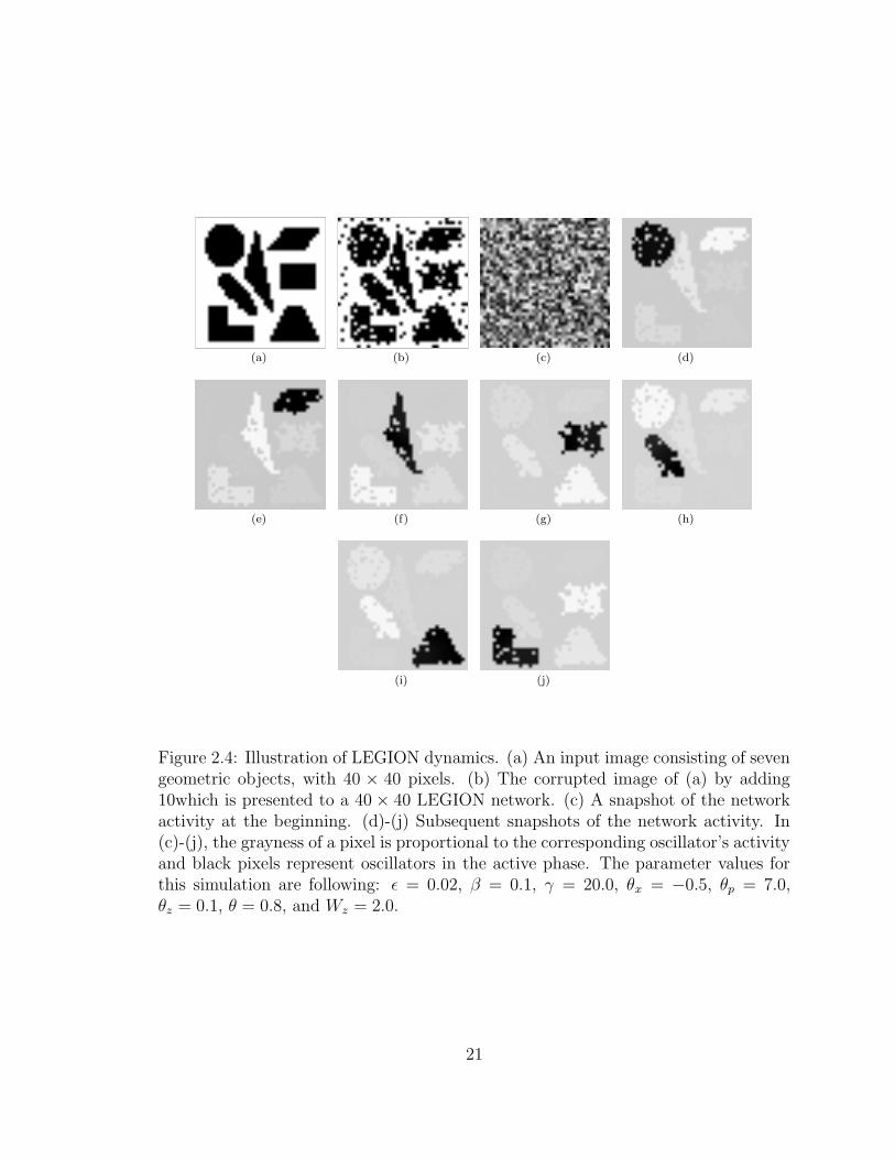
(a) (b) (c) (d)
(e) (f) (g) (h)
(i) (j)
Figure 2.4: Illustration of LEGION dynamics. (a) An input image consisting of sevengeometric objects, with 40 × 40 pixels. (b) The corrupted image of (a) by adding10which is presented to a 40 × 40 LEGION network. (c) A snapshot of the networkactivity at the beginning. (d)-(j) Subsequent snapshots of the network activity. In(c)-(j), the grayness of a pixel is proportional to the corresponding oscillator’s activityand black pixels represent oscillators in the active phase. The parameter values forthis simulation are following: ε = 0.02, β = 0.1, γ = 20.0, θx = −0.5, θp = 7.0,θz = 0.1, θ = 0.8, and Wz = 2.0.
21

Circle
Parallelogram
Triangle
Rectangle
Ellipse
Trapezoid
Staircase
Background
Inhibitor
Time
Figure 2.5: Temporal evolution of the LEGION network. The upper seven plotsshow the combined temporal activities of the seven oscillator blocks representing thecorresponding geometric objects. The eighth plot shows the temporal activities of allthe stimulated oscillators which correspond to the background. The bottom one showsthe temporal activity of the global inhibitor. The simulation took 20,000 integrationsteps using a fourth-order Runge-Kutta method to solve differential equations.
22
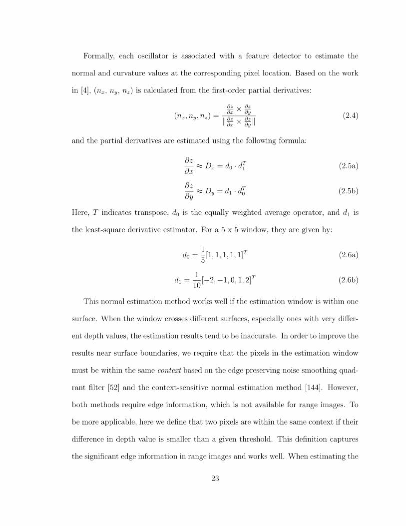
Formally, each oscillator is associated with a feature detector to estimate the
normal and curvature values at the corresponding pixel location. Based on the work
in [4], (nx, ny, nz) is calculated from the first-order partial derivatives:
(nx, ny, nz) =∂z∂x× ∂z
∂y
‖ ∂z∂x× ∂z
∂y‖ (2.4)
and the partial derivatives are estimated using the following formula:
∂z
∂x≈ Dx = d0 · dT
1 (2.5a)
∂z
∂y≈ Dy = d1 · dT
0 (2.5b)
Here, T indicates transpose, d0 is the equally weighted average operator, and d1 is
the least-square derivative estimator. For a 5 x 5 window, they are given by:
d0 =1
5[1, 1, 1, 1, 1]T (2.6a)
d1 =1
10[−2,−1, 0, 1, 2]T (2.6b)
This normal estimation method works well if the estimation window is within one
surface. When the window crosses different surfaces, especially ones with very differ-
ent depth values, the estimation results tend to be inaccurate. In order to improve the
results near surface boundaries, we require that the pixels in the estimation window
must be within the same context based on the edge preserving noise smoothing quad-
rant filter [52] and the context-sensitive normal estimation method [144]. However,
both methods require edge information, which is not available for range images. To
be more applicable, here we define that two pixels are within the same context if their
difference in depth value is smaller than a given threshold. This definition captures
the significant edge information in range images and works well. When estimating the
23
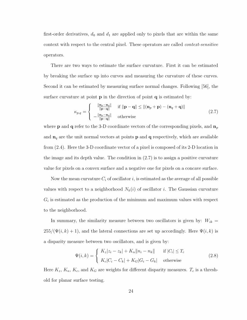
first-order derivatives, d0 and d1 are applied only to pixels that are within the same
context with respect to the central pixel. These operators are called context-sensitive
operators.
There are two ways to estimate the surface curvature. First it can be estimated
by breaking the surface up into curves and measuring the curvature of these curves.
Second it can be estimated by measuring surface normal changes. Following [56], the
surface curvature at point p in the direction of point q is estimated by:
κp,q =
‖np−nq‖‖p−q‖
if ‖p− q‖ ≤ ‖(np + p)− (nq + q)‖
−‖np−nq‖‖p−q‖
otherwise(2.7)
where p and q refer to the 3-D coordinate vectors of the corresponding pixels, and np
and nq are the unit normal vectors at points p and q respectively, which are available
from (2.4). Here the 3-D coordinate vector of a pixel is composed of its 2-D location in
the image and its depth value. The condition in (2.7) is to assign a positive curvature
value for pixels on a convex surface and a negative one for pixels on a concave surface.
Now the mean curvature Ci of oscillator i, is estimated as the average of all possible
values with respect to a neighborhood Nk(i) of oscillator i. The Gaussian curvature
Gi is estimated as the production of the minimum and maximum values with respect
to the neighborhood.
In summary, the similarity measure between two oscillators is given by: Wik =
255/(Ψ(i, k) + 1), and the lateral connections are set up accordingly. Here Ψ(i, k) is
a disparity measure between two oscillators, and is given by:
Ψ(i, k) =
Kz|zi − zk|+Kn‖ni − nk‖ if |Ci| ≤ Tc
Kc|Ci − Ck|+KG|Gi −Gk| otherwise(2.8)
Here Kz, Kn, Kc, and KG are weights for different disparity measures. Tc is a thresh-
old for planar surface testing.
24

2.4 Experimental Results
For real images with a large number of pixels, it involves very intensive numerical
computation to solve the differential equations of (2.1) - (2.3) if the LEGION network
is applied directly. To reduce the numerical computation on a serial computer, an
algorithm is extracted from these equations [135]. The algorithm follows the ma-
jor steps of the original network and exhibits the essential properties of relaxation
oscillator networks. It has been applied to intensity image segmentation [135].
2.4.1 Parameter Selection
Most parameters in (2.1) - (2.3) are intrinsic to LEGION networks and need not
to be changed once they are appropriately chosen, and only the global inhibition Wz
and the potential threshold θp need to be tuned for applications. Other parameters
are application-specific and related to how to measure the similarity between feature
vectors. Theoretically, best parameter values could be obtained through training
using a neural network. Experimentally, each parameter roughly corresponds to a
threshold for a type of discontinuity, and can be set accordingly. In (2.8), Kz captures
abrupt changes in depth, andKn andKc andKG capture boundaries between different
type surfaces.
There are several local windows involved. The system is not sensitive to the size
of windows and can be chosen from a wide range. For the experiments in this work,
we use a single system configuration. That is, the surface normal is estimated from
a 5 × 5 neighboring window, the curvatures are estimated from a 3 × 3 neighboring
window, and each oscillator has lateral connections with its eight immediate neighbors
as depicted in Figure 2.3.
25
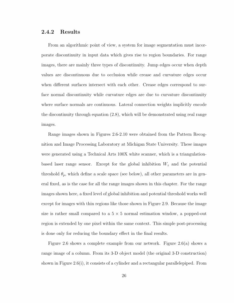
2.4.2 Results
From an algorithmic point of view, a system for image segmentation must incor-
porate discontinuity in input data which gives rise to region boundaries. For range
images, there are mainly three types of discontinuity. Jump edges occur when depth
values are discontinuous due to occlusion while crease and curvature edges occur
when different surfaces intersect with each other. Crease edges correspond to sur-
face normal discontinuity while curvature edges are due to curvature discontinuity
where surface normals are continuous. Lateral connection weights implicitly encode
the discontinuity through equation (2.8), which will be demonstrated using real range
images.
Range images shown in Figures 2.6-2.10 were obtained from the Pattern Recog-
nition and Image Processing Laboratory at Michigan State University. These images
were generated using a Technical Arts 100X white scanner, which is a triangulation-
based laser range sensor. Except for the global inhibition Wz and the potential
threshold θp, which define a scale space (see below), all other parameters are in gen-
eral fixed, as is the case for all the range images shown in this chapter. For the range
images shown here, a fixed level of global inhibition and potential threshold works well
except for images with thin regions like those shown in Figure 2.9. Because the image
size is rather small compared to a 5 × 5 normal estimation window, a popped-out
region is extended by one pixel within the same context. This simple post-processing
is done only for reducing the boundary effect in the final results.
Figure 2.6 shows a complete example from our network. Figure 2.6(a) shows a
range image of a column. From its 3-D object model (the original 3-D construction)
shown in Figure 2.6(i), it consists of a cylinder and a rectangular parallelepiped. From
26

the view point where the image is taken, four planar surfaces and a cylindrical one are
visible. One planar surface is missing from the range image due to sampling artifact
and shadows. Figures 2.6(b)-2.6(f) show the output of the LEGION network. We
can see that all the visible surface regions in the image, including the background,
are popped up. Oscillators belonging to the same surface region are synchronized
due to the strong lateral connections resulting from similar feature vectors and thus
are grouped together correctly. The segregation of these regions is achieved because
of the weak lateral connections resulting from jump and crease edges. Figure 2.6(g)
shows the overall result by putting the popped up regions together into a gray map
[135], where each region is shown using a single gray level. The boundaries between
different surfaces are shown fairly accurately, demonstrating that surface discontinuity
is effectively captured through lateral connection. Small holes in Figure 2.6(d) and
2.6(g) are due to some noise in the input range image. Here Figure 2.6(h), the
intensity image, is included for discussion in Section V.
Figures 2.7 and 2.8 show the segmentation results for a number of more real range
images, which include different types of edges and junctions. These results were
produced using the same parameter values as in Figure 2.6. In Figure 2.7(a), an
object with only planar surfaces is segmented into four surface regions. Boundaries
between surfaces are precisely marked, showing crease edges between planar surfaces
are correctly represented. The junction point where three surfaces intersect is han-
dled correctly without additional modeling, which would be difficult for edge-based
approaches. Figure 2.7(b) shows an object with several planar surfaces and a cylin-
drical one. As in Figure 2.7(a), all the planar surfaces are segmented out precisely.
The cylindrical surface is segmented out correctly even though it is not complete
27
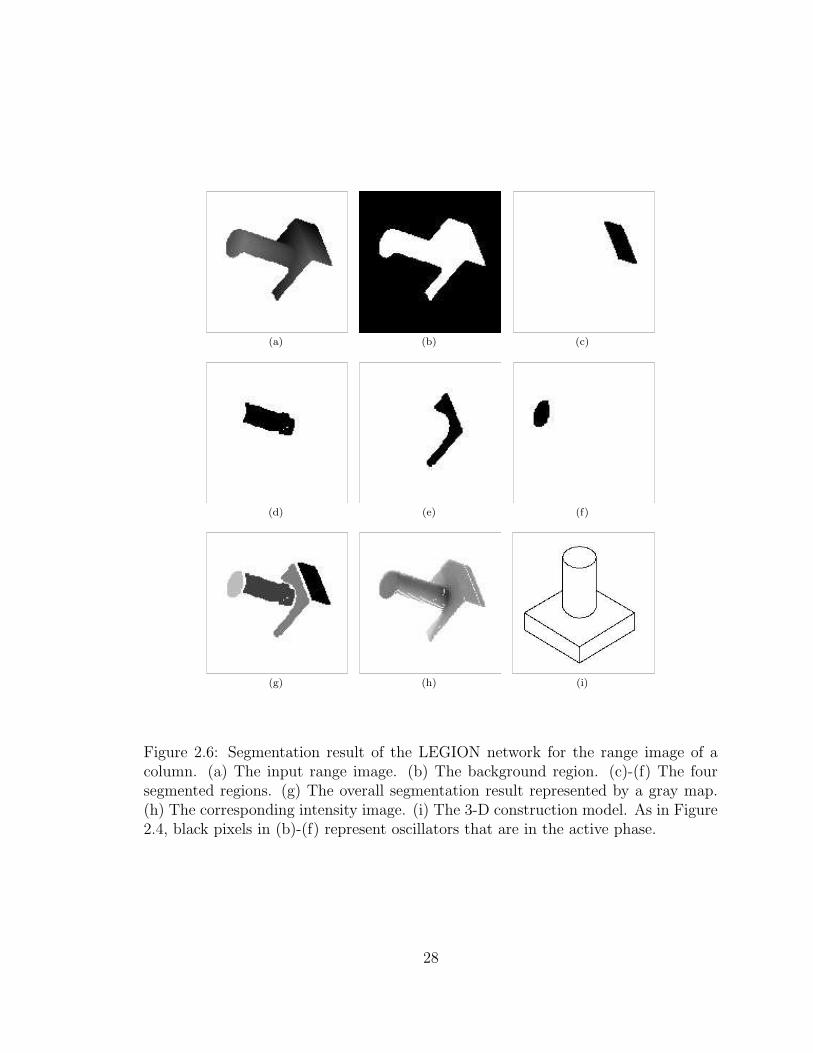
(a) (b) (c)
(d) (e) (f)
(g) (h) (i)
Figure 2.6: Segmentation result of the LEGION network for the range image of acolumn. (a) The input range image. (b) The background region. (c)-(f) The foursegmented regions. (g) The overall segmentation result represented by a gray map.(h) The corresponding intensity image. (i) The 3-D construction model. As in Figure2.4, black pixels in (b)-(f) represent oscillators that are in the active phase.
28
because of shadowing effect. Both jump and crease edges are marked correctly in
the result. Figure 2.7(c) shows an image which consists of two objects. All the sur-
faces are correctly segmented out. Figure 2.7(d) shows a cylinder. The transition
between two surfaces is smoothing and it is even difficult to segment it manually.
The system correctly segmented two surface regions out and the boundary between
them is marked where we would expect. Figure 2.8(a) shows another image with
smoothing transition. Because of that, curvatures were used to segregate the surface
regions. Figure 2.8(b) shows a funnel. Even though the neck is a thin surface, it is
segmented out correctly. But boundary effect is more obvious. Figures 2.8(a) and
2.8(b) demonstrated that the system can handle conic surfaces. Figure 2.8(c) showed
that the network can handle spherical surfaces.
Figure 2.9 shows two difficult examples with thin regions compared to the size of
the normal estimation windows. When using the same parameters as in Figures 2.7
and 2.8, the results are not very satisfactory. This is because the thin parts do not
contain a leader and the normal and curvature estimations are not very reliable due to
the smoothing transitions between surfaces. When tuning the potential threshold and
global inhibition, both images are processed correctly. All the surfaces are segmented
out with boundaries marked correctly, as shown in Figure 2.9.
These examples show clearly that the LEGION network can handle planar, cylin-
drical, conic, and spherical surfaces and different types of surface discontinuity. Only
a few parameters need to be tuned for all these images, which demonstrates that our
network is a robust approach to range image segmentation.
29

(a)
(b)
(c)
(d)
Figure 2.7: Segmentation results of the LEGION network for range images. In eachrow, the left frame shows the input range image, the middle one shows the segmenta-tion result represented by a gray map, and the right one shows the 3-D constructionmodel for comparison purposes.
30
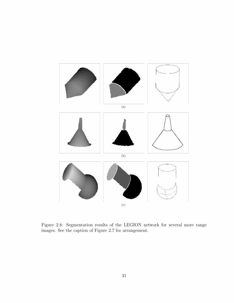
(a)
(b)
(c)
Figure 2.8: Segmentation results of the LEGION network for several more rangeimages. See the caption of Figure 2.7 for arrangement.
31
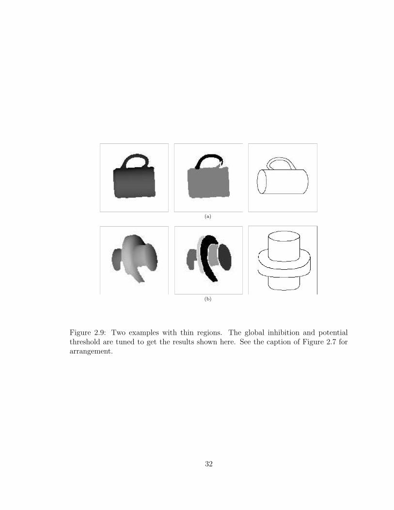
(a)
(b)
Figure 2.9: Two examples with thin regions. The global inhibition and potentialthreshold are tuned to get the results shown here. See the caption of Figure 2.7 forarrangement.
32

2.4.3 Comparison with Existing Approaches
As demonstrated using real range images, lateral connections in our LEGION net-
work capture different types of discontinuity as well as similarity within each surface
region. Both factors are critically important for correct segmentation. Discontinuity
avoids under-segmentation while similarity avoids over-segmentation. Critical points,
such as junctions between surfaces are handled correctly due to the context-sensitive
estimation. These factors determine that our method is close to edge-based ap-
proaches [91][6][136]. For region- and classification-based approaches [49][4][71][67][5],
because in most cases many unspecified parameters and pre- and post-processing are
involved, a quantitative comparison suggested by Hoover et al. [51] is not possible. A
qualitative comparison for similar images is used instead, which may be suggestive.
For the range images used in this chapter, we believe that our results in general are
comparable with the best results from other methods. For the two images whose
similar versions are also used elsewhere, we give a more detailed comparison below.
Cup images similar to Figure 2.9(a) were also used in [49][4][71]. In [49], a cup
image was first classified into two patch images through three different tests. The
two patch images were merged to form another patch image, based on which the
final classification was generated. In the final result, the handle was classified as
background, resulting in wrong topology. In [4], a coffee mug was segmented into six
bivariate polynomial surfaces with complicated coefficients, which were obtained by
surface fitting after curvature-based initial classification. The handle was incorrectly
segmented into two surfaces. In [24], a slightly different cup image was segmented in
five parts through an iterative regression method, where the handle was broken into
three parts. In our case, Figure 2.9(a) shows that the cup was segmented correctly into
33

two regions, the body and the handle. This qualitative comparison suggests that only
our approach produced a correct segmentation, without under- or over-segmentation.
An image similar to Figure 2.6(a) was also used in [5]. At the lower layers of
the hierarchical network, the image was broken into small patches because a position
term, not relevant to surface properties, is included in the feature vector in order to
achieve spatial connectivity [67][5]. Due to the position term, even planar surfaces
need several layers to be correctly segmented. More complicated surfaces, such as
cylindrical and conic ones, tend to be broken into small regions. As shown in [5],
an image may be correctly classified only when the correct number of regions in a
layer is given. This problem is not solved even using a hierarchical network. To
produce meaningful results, segmentation from different layers must be combined.
Because of that, this neural network based approaches [67][5] in general became a
split-and-merge algorithm.
Methodologically, our approach has several major advantages over other methods.
Firstly, the segmentation result is the emergent behavior of the LEGION network; the
flexible representation of temporal labeling promises to provide a generic solution to
image segmentation. Different cues, such as depth and color (see Figures 2.6(a) and
2.6(h)) are highly correlated and should be integrated to improve the performance
of a machine vision system. LEGION provides a unified and effective framework to
implement the integration through lateral connections. On the other hand, the inte-
gration would be difficult for segmentation algorithms [56][49][4][136][67][5]; different
information must be modeled explicitly and encoded accordingly. Secondly, due to
the non-linearity of single oscillators and the effective architecture for modeling local
and global coupling, our network is guaranteed to converge very efficiently. To our
34

best knowledge, this is the only oscillatory network that has been analyzed rigorously.
Finally, our approach is a dynamical system with parallel and distributed computa-
tion. The unique property of neural plausibility makes it particularly feasible for
analog VLSI implementation, the efficiency of which may pave the way to achieve
real-time range image segmentation.
2.5 Discussions
A LEGION network has been constructed and applied to range image segmenta-
tion. Our network successfully segments real range images, which shows that it may
give rise to a generic range image segmentation method.
2.5.1 Biological Plausibility of the Network
The relaxation oscillator used in LEGION is similar to many oscillators used in
modeling neuronal behaviors, including FitzHugh-Nagumo [31][96] and Morris-Lecar
model [93], and is reducible from the Hodgkin-Huxley equations [48]. The local
excitatory connections are consistent with various lateral connections in the brain
and can be viewed as the horizontal connections in the visual cortex [37]. The global
inhibitor, which receives input from the entire network and feeds back with inhibition,
can be viewed as a network that exerts some form of global control. Oscillatory
correlation, as a special form of temporal correlation [90][130], also conforms with
experiments of stimulus-dependent oscillations, where synchronous oscillations occur
when the stimulus is a coherent object, and no phase locking exists when regions are
stimulated by different stimuli [26][40][116].
As stated earlier, the LEGION network can produce segmentation results within
a few cycles. This analytical result may suggest a striking agreement with human
35
performance in perceptual organization. It is well-known that human subjects can
perform segmentation (figure-ground segregation) tasks in a small fraction of a second
[7], corresponding to several cycles of oscillations if the frequency is taken to be around
40 Hz as commonly reported. Thus, if our oscillator network is implemented in real-
time hardware, the time it takes the network to perform a segmentation task would
be compatible with human performance.
2.5.2 Comparison with Pulse-Coupled Neural Networks
Both LEGION and PCNN networks were proposed based on the temporal cor-
relation theory [90][130] and experimental data of stimulus-dependent oscillations
[26][40]. Single units in both models approximate nonlinear neuronal activity, and
excitatory local coupling is used to achieve synchronization. These are similarities
between them. Yet there are important differences.
A single neuron in PCNN networks consists of input units, a linking modulation,
and a pulse generator, all of which are mainly implemented using leaky integrators
[27]. The input units consist of two principal branches, called feeding and linking
inputs. Feeding inputs are the primary inputs from the neuron’s receptive field while
linking inputs are mainly the lateral connections with neighboring neurons and may
also include feedback controls from higher layers. The linking modulation modulates
the feeding inputs with linking inputs and produces the total internal activity U ,
which is given by U = F (1 + βL). Here F and L are total feeding and linking
inputs respectively, and β is a parameter that controls the linking strength. The
pulse generator is a Heaviside function of the difference between the total internal
activity and a dynamic threshold implemented through another leaky integrator. If
36
β is set to zero, the neuron becomes an encoder, which maps the intensity linearly
to firing frequency. If the activities from all neurons are summed up, the resulting
output is a time series, which corresponds to the histogram of the input image [59].
With linking inputs, the behavior of the network can be very complicated. But
when β is small, corresponding to the weak linking regime [59], synchronization is
achieved only when the differences are small, similar to a smoothing operation. This
type of PCNN can transform the input image into firing frequency representation
with desirable invariant properties [59]. Variations of this type of PCNN have found
successful applications in image factorization [60] and may have a connection with
wavelet and other transformations [103].
Recently, Stoecker et al. [120] also applied PCNN to scene segmentation. The
network successfully separated identical objects in a visual scene. Because differ-
ent intensities map to different firing frequencies, the network would have difficulty
in handling real images. For real images, different objects generally correspond to
different frequencies, and the readout would be problematic, i.e., it would be diffi-
cult to have a network that could detect the segmentation. More fundamentally, the
interactions among different firing frequencies have not been investigated. In [120],
desynchronization is achieved solely due to the spatial distances among input objects.
On the other hand, LEGION networks can successfully segment real range images as
demonstrated here and other real images such as texture images [16].
Another difference is that LEGION has a well-analyzed mathematical foundation
[123][135] whereas there is little analytical investigation on PCNN probably because
37
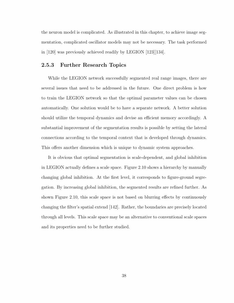
the neuron model is complicated. As illustrated in this chapter, to achieve image seg-
mentation, complicated oscillator models may not be necessary. The task performed
in [120] was previously achieved readily by LEGION [123][134].
2.5.3 Further Research Topics
While the LEGION network successfully segmented real range images, there are
several issues that need to be addressed in the future. One direct problem is how
to train the LEGION network so that the optimal parameter values can be chosen
automatically. One solution would be to have a separate network. A better solution
should utilize the temporal dynamics and devise an efficient memory accordingly. A
substantial improvement of the segmentation results is possible by setting the lateral
connections according to the temporal context that is developed through dynamics.
This offers another dimension which is unique to dynamic system approaches.
It is obvious that optimal segmentation is scale-dependent, and global inhibition
in LEGION actually defines a scale space. Figure 2.10 shows a hierarchy by manually
changing global inhibition. At the first level, it corresponds to figure-ground segre-
gation. By increasing global inhibition, the segmented results are refined further. As
shown Figure 2.10, this scale space is not based on blurring effects by continuously
changing the filter’s spatial extend [142]. Rather, the boundaries are precisely located
through all levels. This scale space may be an alternative to conventional scale spaces
and its properties need to be further studied.
38
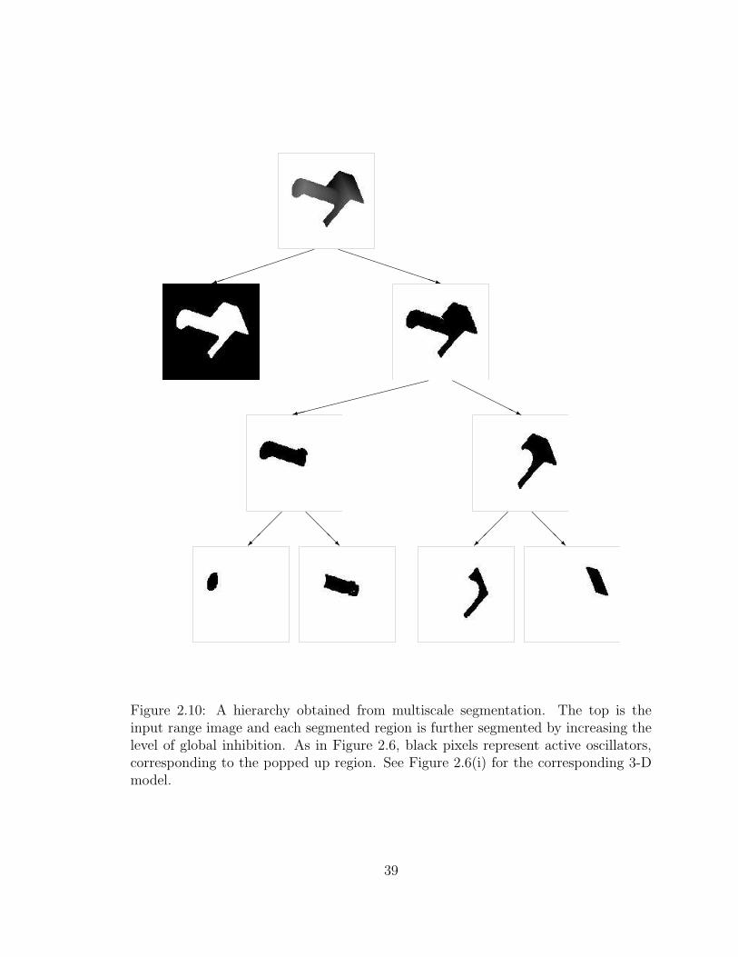
)
PPPPPPPPPq
9
HHHHHHj
@@
@R
@@
@R
Figure 2.10: A hierarchy obtained from multiscale segmentation. The top is theinput range image and each segmented region is further segmented by increasing thelevel of global inhibition. As in Figure 2.6, black pixels represent active oscillators,corresponding to the popped up region. See Figure 2.6(i) for the corresponding 3-Dmodel.
39

CHAPTER 3
BOUNDARY DETECTION BY CONTEXTUAL
NONLINEAR SMOOTHING
In this chapter we present a two-step boundary detection algorithm. The first
step is a nonlinear smoothing algorithm which is based on an orientation-sensitive
probability measure. By incorporating geometrical constraints through the coupling
structure, we obtain a robust nonlinear smoothing algorithm, where many nonlin-
ear algorithms can be derived as special cases. Even when noise is substantial, the
proposed smoothing algorithm can still preserve salient boundaries. Compared with
anisotropic diffusion approaches, the proposed nonlinear algorithm not only performs
better in preserving boundaries but also has a non-uniform stable state, whereby re-
liable results are available within a fixed number of iterations independent of images.
The second step is simply a Sobel edge detection algorithm without non-maximum
suppression and hysteresis tracking. Due to the proposed nonlinear smoothing, salient
boundaries are extracted effectively. Experimental results using synthetic and real
images are provided. The results presented in this chapter appeared in [79] [80].
40
3.1 Introduction
One of the fundamental tasks in low-level machine vision is to locate discontinu-
ities in images corresponding to physical boundaries between a number of regions. A
common practice is to identify local maxima in local gradients of images - collectively
known as edge detection algorithms. The Sobel edge detector [14] consists of two 3
x 3 convolution kernels, which respond maximally to vertical and horizontal edges
respectively. Local gradients are estimated by convolving the images with the two
kernels, and thresholding is then applied to get rid of noisy responses. The Sobel
edge detector is computationally efficient but sensitive to noise. To make the esti-
mation of gradients more reliable, the image can be convolved with a low-pass filter
before estimation and two influential methods are due to Marr and Hildreth [89] and
Canny [13]. By convolving the image with a Laplacian of Gaussian kernel, the re-
sulting local maxima, which are assumed to correspond to meaningful edge points,
are zero-crossings in the filtered image [89]. Canny [13] derived an optimal step edge
detector using variational techniques starting from some optimal criteria and used the
first derivative of a Gaussian as a good approximation of the derived detector. Edge
points are then identified using a non-maximum suppression and hysteresis thresh-
olding for better continuity of edges. As noticed by Marr and Hildreth [89], edges
detected at a fixed scale are not sufficient and multiple scales are essentially needed
in order to obtain good results. By formalizing the multiple scale approach, Witkin
[142] and Koenderink [66] proposed Gaussian scale space. The original image is em-
bedded in a family of gradually smoothing images controlled by a single parameter,
which is equivalent to solving a heat equation with input as the initial condition [66].
While Gaussian scale space has nice properties and is widely used in machine vision
41
[75], a major limitation is that Gaussian smoothing inevitably blurs edges and other
important features due to its low-pass nature. To overcome the limitation, anisotropic
diffusion, which was proposed by Cohen and Grossberg [19] in modeling the primary
visual cortex, was formulated by Perona and Malik [105]:
∂I
∂t= div(g(‖∇‖)∇I) (3.1)
Here div is the divergence operator, and g is a nonlinear monotonically decreasing
function and ∇I denotes the gradient. By making the diffusion conductance depen-
dent explicitly on local gradients, anisotropic diffusion prefers intra-region smoothing
over inter-region smoothing, resulting immediate localization while noise is reduced
[105]. Because it produces visually impressive results, anisotropic diffusion gener-
ates much theoretical as well as practical interest (see reference [138] for a recent
review). While many improvements have been proposed, including spatial regular-
ization [137] and edge-enhancing anisotropic diffusion [15], the general framework
remains the same. As shown by You et al. [145], anisotropic diffusion given by (3.1)
is the steepest gradient descent minimizer of the following energy function:
E(I) =∫
Ωf(‖∇‖)dΩ (3.2)
with
g(‖∇‖) = f ′(‖∇‖)‖∇‖
Under some general conditions, the energy function given by (3.2) has a unique and
trivial global minimum, where the image is constant everywhere, and thus interest-
ing results exist only within a certain period of diffusion. An immediate problem is
how to determine the termination time, which we refer to as the termination prob-
lem. While there are some heuristic rules on how to choose the stop time [137] [15],
42

in general it corresponds to the open problem of automatic scale selection. As in
Gaussian scale space, a fixed time would not be sufficient to obtain good results.
Another problem of anisotropic diffusion is that diffusion conductance is a determin-
istic function of local gradients, which, similar to non-maximum suppression in edge
detection algorithms, makes an implicit assumption that larger gradients are due to
true boundaries. When noise is substantial and gradients due to noise and boundaries
cannot be distinguished based on magnitudes, the approach tends to fail to preserve
meaningful region boundaries.
To illustrate the problems, Figure 3.1(a) shows a noise-free image, where the gra-
dient magnitudes along the central square change considerably. Figure 3.1(b) shows a
noisy version of Figure 3.1(a) by adding Gaussian noise with zero mean and σ = 40,
and Figure 3.1(c) shows its local gradient magnitude obtained using Sobel opera-
tors [14]. While the three major regions in Figure 3.1(b) may be perceived, Figure
3.1(c) is very noisy and the strong boundary fragment is barely visible. Figures 3.1
(d)-(f) show the smoothed images by an anisotropic diffusion algorithm [106] with
specified numbers of iterations. Figures 3.1 (g)-(i) show the edge maps of Figure 3.1
(d)-(f), respectively, using the Sobel edge detection algorithm. While at the 50th
iteration the result is still noisy, the result becomes meaningless at the 1000th itera-
tion. Even though the result at the 100th iteration is visually good, the boundaries
are still fragmented and it is not clear how to identify a ”good” number of iterations
automatically.
These problems to a large extent are due to the assumption that local maxima in
gradient images are good edge points. In other words, due to noise, responses from
true boundaries and those from noise are not distinguishable based on magnitude.
43

(a) (b) (c)
(d) (e) (f)
(g) (h) (i)
Figure 3.1: An example with non-uniform boundary gradients and substantialnoise. (a) A noise-free synthetic image. Gray values in the image: 98 for the left ‘[’region, 138 for the square, 128 for the central oval, and 158 for the right ‘]’ region.(b) A noisy version of (a) with Gaussian noise of σ = 40. (c) Local gradient map of(b) using the Sobel operators. (d)-(f) Smoothed images from an anisotropic diffusionalgorithm [106] at 50, 100, and 1000 iterations. (g)-(i) Corresponding edge maps of(d)-(f) respectively using the Sobel edge detector.
44
To overcome these problems, contextual information, i.e., responses from neighboring
pixels, should be incorporated in order to reduce ambiguity as in relaxation labeling
and related methods [112] [55] [72] [42]. In general, relaxation labeling methods use
pair-wise compatibility measure, which is determined based on a priori models asso-
ciated with labels, and convergence is not known and often very slow in numerical
simulations[88]. In this chapter, by using an orientation-sensitive probability mea-
sure, we incorporate contextual information through the geometrical constraints on
the coupling structure. Numerical simulations show that the resulting nonlinear al-
gorithm has a non-uniform stable state and good results can be obtained within a
fixed number of iterations independent of input images. Also, the oriented probability
measure is defined on input data, and thus no a priori models need to be assumed.
In Section 3.2, we formalize our contextual nonlinear smoothing algorithm and
show that many nonlinear smoothing algorithms can be treated as special cases.
Section 3.3 gives some theoretical results as well as numerical simulations regarding
to the stability and convergence of the algorithm. Section 3.4 provides experimental
results using synthetic and real images. Section 3.5 concludes the chapter with further
discussions.
3.2 Contextual Nonlinear Smoothing Algorithm
3.2.1 Design of the Algorithm
To design a statistical algorithm, with no prior knowledge, we assume a Gaussian
distribution within each region. That is, given a pixel (i0, j0) and a window R(i0,j0)
at pixel (i0, j0), consisting of a set of pixel locations, we assume that:
P (I(i0,j0), R) =1√
2πσR
exp
−(I(i0,j0) − µR)2
2σ2R
(3.3)
45
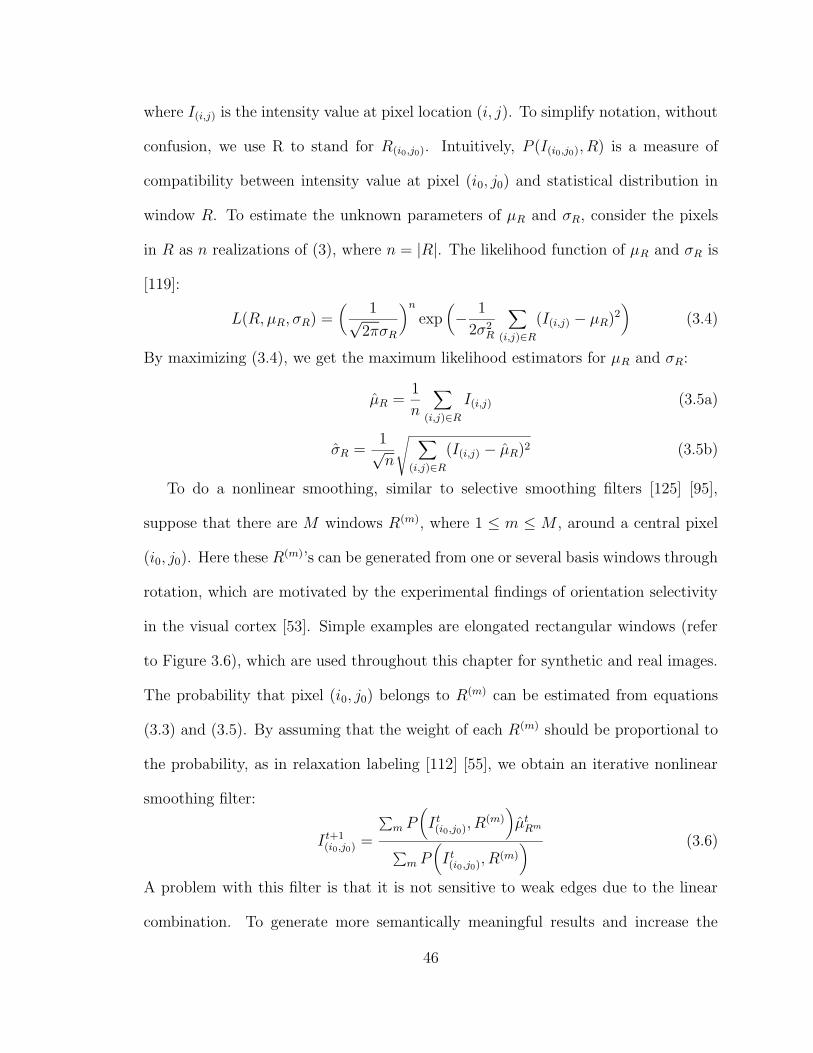
where I(i,j) is the intensity value at pixel location (i, j). To simplify notation, without
confusion, we use R to stand for R(i0,j0). Intuitively, P (I(i0,j0), R) is a measure of
compatibility between intensity value at pixel (i0, j0) and statistical distribution in
window R. To estimate the unknown parameters of µR and σR, consider the pixels
in R as n realizations of (3), where n = |R|. The likelihood function of µR and σR is
[119]:
L(R, µR, σR) =(
1√2πσR
)n
exp(
− 1
2σ2R
∑
(i,j)∈R
(I(i,j) − µR)2)
(3.4)
By maximizing (3.4), we get the maximum likelihood estimators for µR and σR:
µR =1
n
∑
(i,j)∈R
I(i,j) (3.5a)
σR =1√n
√
∑
(i,j)∈R
(I(i,j) − µR)2 (3.5b)
To do a nonlinear smoothing, similar to selective smoothing filters [125] [95],
suppose that there are M windows R(m), where 1 ≤ m ≤ M , around a central pixel
(i0, j0). Here these R(m)’s can be generated from one or several basis windows through
rotation, which are motivated by the experimental findings of orientation selectivity
in the visual cortex [53]. Simple examples are elongated rectangular windows (refer
to Figure 3.6), which are used throughout this chapter for synthetic and real images.
The probability that pixel (i0, j0) belongs to R(m) can be estimated from equations
(3.3) and (3.5). By assuming that the weight of each R(m) should be proportional to
the probability, as in relaxation labeling [112] [55], we obtain an iterative nonlinear
smoothing filter:
I t+1(i0,j0) =
∑
m P(
I t(i0,j0), R
(m)
)
µtRm
∑
m P(
I t(i0,j0), R
(m)
) (3.6)
A problem with this filter is that it is not sensitive to weak edges due to the linear
combination. To generate more semantically meaningful results and increase the
46
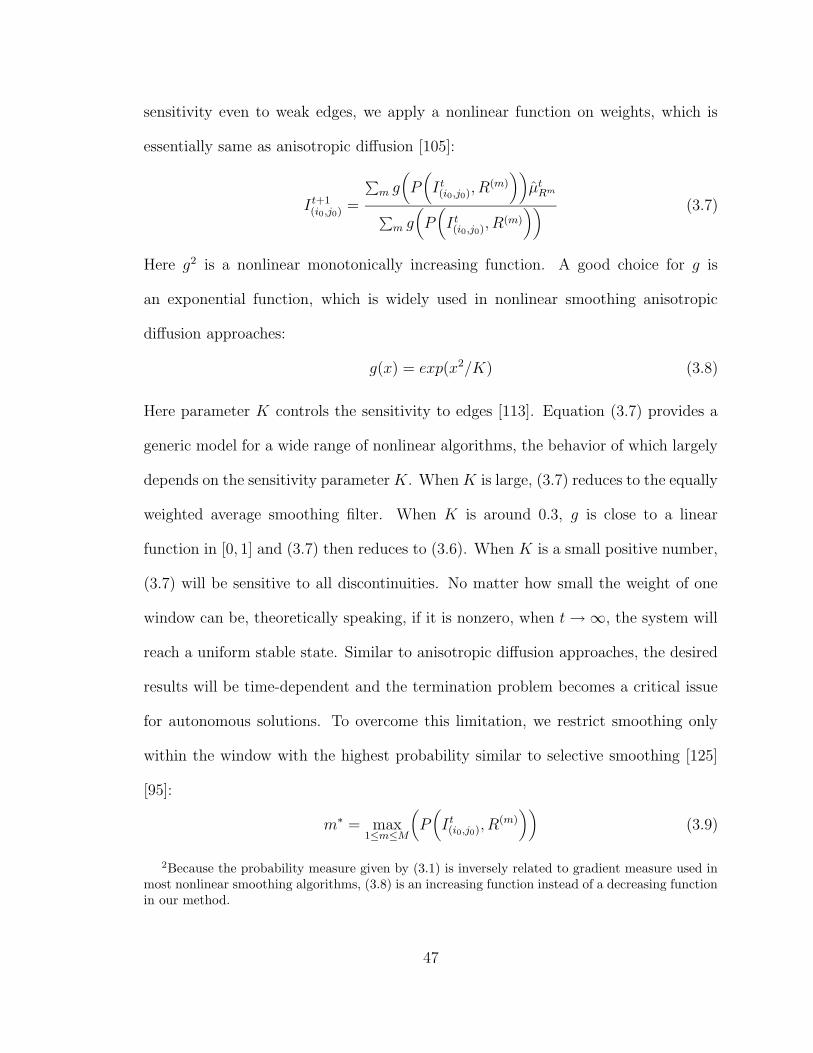
sensitivity even to weak edges, we apply a nonlinear function on weights, which is
essentially same as anisotropic diffusion [105]:
I t+1(i0,j0) =
∑
m g(
P(
I t(i0,j0), R
(m)
))
µtRm
∑
m g(
P(
I t(i0,j0), R
(m)
)) (3.7)
Here g2 is a nonlinear monotonically increasing function. A good choice for g is
an exponential function, which is widely used in nonlinear smoothing anisotropic
diffusion approaches:
g(x) = exp(x2/K) (3.8)
Here parameter K controls the sensitivity to edges [113]. Equation (3.7) provides a
generic model for a wide range of nonlinear algorithms, the behavior of which largely
depends on the sensitivity parameterK. WhenK is large, (3.7) reduces to the equally
weighted average smoothing filter. When K is around 0.3, g is close to a linear
function in [0, 1] and (3.7) then reduces to (3.6). When K is a small positive number,
(3.7) will be sensitive to all discontinuities. No matter how small the weight of one
window can be, theoretically speaking, if it is nonzero, when t→∞, the system will
reach a uniform stable state. Similar to anisotropic diffusion approaches, the desired
results will be time-dependent and the termination problem becomes a critical issue
for autonomous solutions. To overcome this limitation, we restrict smoothing only
within the window with the highest probability similar to selective smoothing [125]
[95]:
m∗ = max1≤m≤M
(
P(
I t(i0,j0), R
(m)))
(3.9)
2Because the probability measure given by (3.1) is inversely related to gradient measure used inmost nonlinear smoothing algorithms, (3.8) is an increasing function instead of a decreasing functionin our method.
47
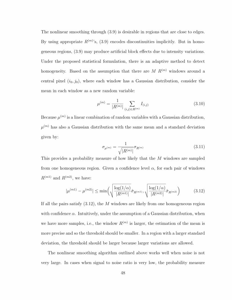
The nonlinear smoothing through (3.9) is desirable in regions that are close to edges.
By using appropriate R(m)’s, (3.9) encodes discontinuities implicitly. But in homo-
geneous regions, (3.9) may produce artificial block effects due to intensity variations.
Under the proposed statistical formulation, there is an adaptive method to detect
homogeneity. Based on the assumption that there are M R(m) windows around a
central pixel (i0, j0), where each window has a Gaussian distribution, consider the
mean in each window as a new random variable:
µ(m) =1
|R(m)|∑
(i,j)∈R(m)
I(i,j) (3.10)
Because µ(m) is a linear combination of random variables with a Gaussian distribution,
µ(m) has also a Gaussian distribution with the same mean and a standard deviation
given by:
σµ(m) =1
√
|R(m)|σR(m) (3.11)
This provides a probability measure of how likely that the M windows are sampled
from one homogeneous region. Given a confidence level α, for each pair of windows
R(m1) and R(m2), we have:
|µ(m1) − µ(m2)| ≤ min(
√
√
√
√
log(1/α)
|R(m1)| σR(m1) ,
√
√
√
√
log(1/α)
|R(m2)| σR(m2)
)
(3.12)
If all the pairs satisfy (3.12), the M windows are likely from one homogeneous region
with confidence α. Intuitively, under the assumption of a Gaussian distribution, when
we have more samples, i.e., the window R(m) is larger, the estimation of the mean is
more precise and so the threshold should be smaller. In a region with a larger standard
deviation, the threshold should be larger because larger variations are allowed.
The nonlinear smoothing algorithm outlined above works well when noise is not
very large. In cases when signal to noise ratio is very low, the probability measure
48
given in (3.3) would be unreliable because pixel values change considerably. This
problem can be alleviated by using the mean value of pixels sampled from R which
are close to the central pixel (i0, j0), or along a certain direction to make the algorithm
more orientation sensitive.
To summarize, we obtain a nonlinear smoothing algorithm. We define M oriented
windows which can be obtained by rotating one or more basis windows. At each pixel,
we estimate parameters using (3.5). If all the M windows belong to a homogeneous
region according to (3.12), we do the smoothing within all theM windows. Otherwise,
the smoothing is done only within the most compatible window given by (3.9).
3.2.2 A Generic Nonlinear Smoothing Framework
In this section we will show how to derive several widely used nonlinear algorithms
from the statistical nonlinear algorithm outlined above. Several early nonlinear filters
[125] [95] do the smoothing in a window where the standard deviation is the smallest.
These filters can be obtained by simplifying (3.3) to:
P (I(i0,j0), µ, σ) =1√2πσ
C (3.13)
where C is a constant. Then the solution to (3.9) is the window with the smallest
deviation. Recently, Higgins and Hsu [47] extended the principle of choosing the
window with the smallest deviation for edge detection.
Another nonlinear smoothing filter is the gradient-inverse filter [131]. Suppose
that there is one window, i.e., M = 1, consisting of the central pixel (i0, j0) itself
only, the estimated deviation for a given pixel (i, j) in (3.5b) now becomes:
σ = |I(i,j) − I(i0,j0)| (3.14)
49
Equation (3.14) is a popular way to estimate local gradients. Using (13) as the
probability measure, (3.6) becomes exactly the gradient inverse nonlinear smoothing
filter [131].
SUSAN nonlinear smoothing filter [117] is proposed based on SUSAN (Smallest
Univalue Segment Assimilating Nucleus) principle. It is formulated as:
I t+1(i0,j0) =
∑
(δi,δj)6=(0,0) It(i0+δi,j0+δj)W (i0, j0, δi, δj)
∑
(δi,δj)6=(0,0)W (i0, j0, δi, δj)(3.15)
where
W (i0, j0, δi, δj) = exp
(
− 12σ2 −
(
It(i0+δi,j0+δj)
−It(i0,j0)
)2
T 2
)
Here (i0, j0) is the central pixel under consideration, and (δi, δj) defines a local neigh-
borhood. Essentially, it integrates Gaussian smoothing in spatial and brightness
domains. The parameter T is a threshold for intensity values. It is easy to see from
(3.15) that the weights are derived based on pair-wise intensity value differences. It
would be expected that the SUSAN filter performs well when images consists of rel-
atively homogeneous regions and within each region noise is smaller than T . When
noise is substantial, it fails to preserve structures due to the pair-wise difference cal-
culation, where no geometrical constraints are incorporated. This is consistent with
the experimental results, which will be discussed later. To get the SUSAN filter, we
define one window including the central pixel itself only. For a given pixel (i, j) in its
neighborhood, (3.3) can be simplified to:
P (I(i,j), R) = C exp(
−(I(i,j),−µR)2
T 2
)
(3.16)
where C is a scaling factor. Because now µR is I(i0,j0), (3.6) with the probability
measure given by (3.16) is equivalent to Gaussian smoothing in the brightness domain
in (3.15).
50

Now consider anisotropic diffusion given by (3.1). By discretizing (3.1) in image
domain with four nearest neighbor coupling [106] and rearranging terms, we have:
I t+1(i,j) = ηt
(i,j)It(i,j) + λ
∑
m
g(P (I t(i,j), R
(m)))µR(m) (3.17)
If we have four singleton regions, (3.17) is essentially a simplified version of (3.7) with
an adaptive learning rate.
3.3 Analysis
3.3.1 Theoretical Results
One of the distinctive characteristics of the proposed algorithm is that it requires
spatial constraints among responses from neighboring locations through coupling
structure as opposed to pair-wise coupling structure. Figure 3.2 illustrates the con-
cept using a manually constructed example. Figure 3.2(a) shows the oriented windows
in a 3 x 3 neighborhood, and Figure 3.2(c) shows the coupling structure if we apply
the proposed algorithm to a small image patch shown in Figure 3.2(b). The directed
graph is constructed as follows. There is a directed edge from (i1, j1) to (i0, j0) if and
only if (i1, j1) contributes to the smoothing of (i0, j0) according to equations (3.12)
and (3.9). By doing so, the coupling structure is represented as a directed graph as
shown in Figure 3.2(c). Connected components and strongly connected components
[20] of the directed graph can be used to analyze the temporal behavior of the pro-
posed algorithm. A strongly connected component is a set of vertices, or pixels here,
where there is a directed path from any vertex to all the other vertices in the set.
We obtain a connected component if we do not consider the direction of edges along
a path. In the example shown in Figure 3.2(c), all the black pixels form a strongly
51
connected component and so do all the white pixels. Also, there are obviously two
connected components.
Essentially our nonlinear smoothing algorithm can be viewed as a discrete dy-
namic system, the behavior of which is complex due to spatial constraints imposed
by coupling windows and adaptive coupling structure by probabilistic grouping. We
now prove that a constant region satisfying certain geometrical constraints is a stable
state of the smoothing algorithm.
Theorem 1. If a region S of a given image I satisfies:
(i1, j1) ∈ S and (i2, j2) ∈ S ⇒ I(i1,j1) = I(i2,j2) (3.18a)
∀(i, j) ∈ S ⇒ ∃mR(m)(i,j) ⊆ S (3.18b)
Then S is stable with respect to the proposed algorithm.
Proof. Condition (3.18a) states that S is a constant region and the standard
deviation is zero if R(m) is within S according to equation (3.5b). Consider a pixel
(i0, j0) in S. Inequality (3.12) is satisfied only when all R(m)’s are within S. In
this case, the smoothing algorithm does not change the intensity value at (i0, j0).
Otherwise, according to equation (3.9) must be within S because there exists at least
one such window according to (3.18b) and thus the smoothing algorithm does not
change the intensity value at (i0, j0) also. So S is stable. Q.E.D.
A maximum connected component of the constructed graph is stable when its
pixels are constant and thus maximum connected components of the constructed
graph are a piecewise constant stable solution of the proposed algorithm. For the
image patch given in Figure 3.2(b), for example, a stable solution is that pixels in
each of the two connected components are constant. The noise-free image in Figure
52

(a)
(b) (c)
Figure 3.2: Illustration of the coupling structure of the proposed algorithm. (a) Eightoriented windows and a fully connected window defined on a 3 x 3 neighborhood. (b)A small synthetic image patch of 6 x 8 in pixels. (c) The resulting coupling structurefor (b). There is a directed edge from (i1, j1) to a neighbor (i0, j0) if and only if (i1, j1)contributes to the smoothing of (i0, j0) according to equations (3.12) and (3.9). Eachcircle represents a pixel, where the inside color is proportional to the gray value ofthe corresponding pixel. Ties in (3.9) are broken according to left-right and top-downpreference of the oriented windows in (a).
53
3.1(a) is also a stable solution by itself, as we will demonstrate through numerical
simulations later on. It is easy to see from the proof that any region which satisfies
conditions (3.18a) and (3.18b) during temporal evolution will stay unchanged. In
addition, due to the smoothing nature of the algorithm, a local maximum at iteration
t cannot increase according to the smoothing kernel by equation (3.12) or (3.9), and
similarly, a local minimum cannot decrease. We conjecture that any given image
approaches an image that is almost covered by homogeneous regions. Due to the
spatial constraints given by (3.18b), it is not clear if the entire image converges to a
piece-wise constant stable state. Within each resulting homogeneous region, (3.18b)
is satisfied and thus the region becomes stable. For pixels near boundaries, corners,
and junctions, it is possible that (18b) is not uniquely satisfied within one constant
region, and small changes may persist. The whole image in this case attains a quasi-
equilibrium state. This is supported by the following numerical simulations using
synthetic and real images. While there are pixels which do not converge within 1000
iterations, the smoothed image as a whole does not change noticeably at all. The two
maximum strongly connected components in Figure 3.2(b) satisfy condition (3.18b).
Both of them are actually uniform regions and thus are stable. Gray pixels would
be grouped into one of the two stable regions according to pixel value similarity and
spatial constraints.
3.3.2 Numerical Simulations
Because it is difficult to derive the speed of convergence analytically, we use nu-
merical simulations to demonstrate the temporal behavior of the proposed algorithm.
Since smoothing is achieved using equally weighted average within selected windows,
54
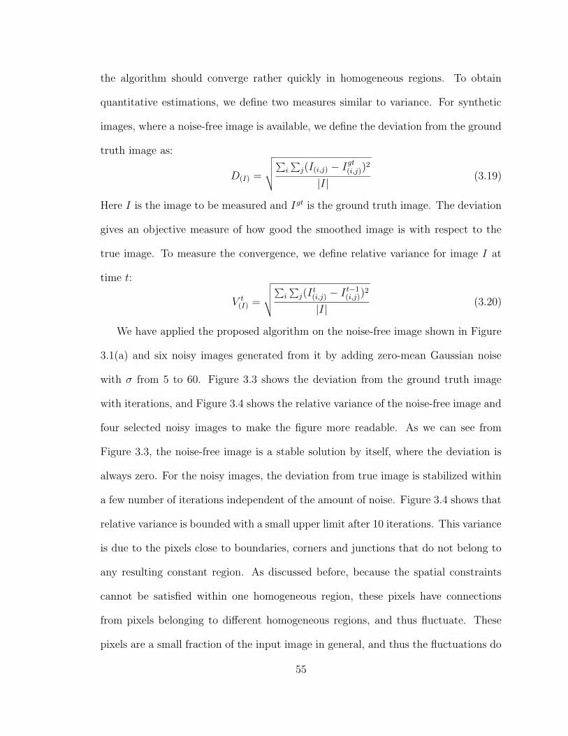
the algorithm should converge rather quickly in homogeneous regions. To obtain
quantitative estimations, we define two measures similar to variance. For synthetic
images, where a noise-free image is available, we define the deviation from the ground
truth image as:
D(I) =
√
√
√
√
∑
i
∑
j(I(i,j) − Igt(i,j))
2
|I| (3.19)
Here I is the image to be measured and Igt is the ground truth image. The deviation
gives an objective measure of how good the smoothed image is with respect to the
true image. To measure the convergence, we define relative variance for image I at
time t:
V t(I) =
√
√
√
√
∑
i
∑
j(It(i,j) − I t−1
(i,j))2
|I| (3.20)
We have applied the proposed algorithm on the noise-free image shown in Figure
3.1(a) and six noisy images generated from it by adding zero-mean Gaussian noise
with σ from 5 to 60. Figure 3.3 shows the deviation from the ground truth image
with iterations, and Figure 3.4 shows the relative variance of the noise-free image and
four selected noisy images to make the figure more readable. As we can see from
Figure 3.3, the noise-free image is a stable solution by itself, where the deviation is
always zero. For the noisy images, the deviation from true image is stabilized within
a few number of iterations independent of the amount of noise. Figure 3.4 shows that
relative variance is bounded with a small upper limit after 10 iterations. This variance
is due to the pixels close to boundaries, corners and junctions that do not belong to
any resulting constant region. As discussed before, because the spatial constraints
cannot be satisfied within one homogeneous region, these pixels have connections
from pixels belonging to different homogeneous regions, and thus fluctuate. These
pixels are a small fraction of the input image in general, and thus the fluctuations do
55
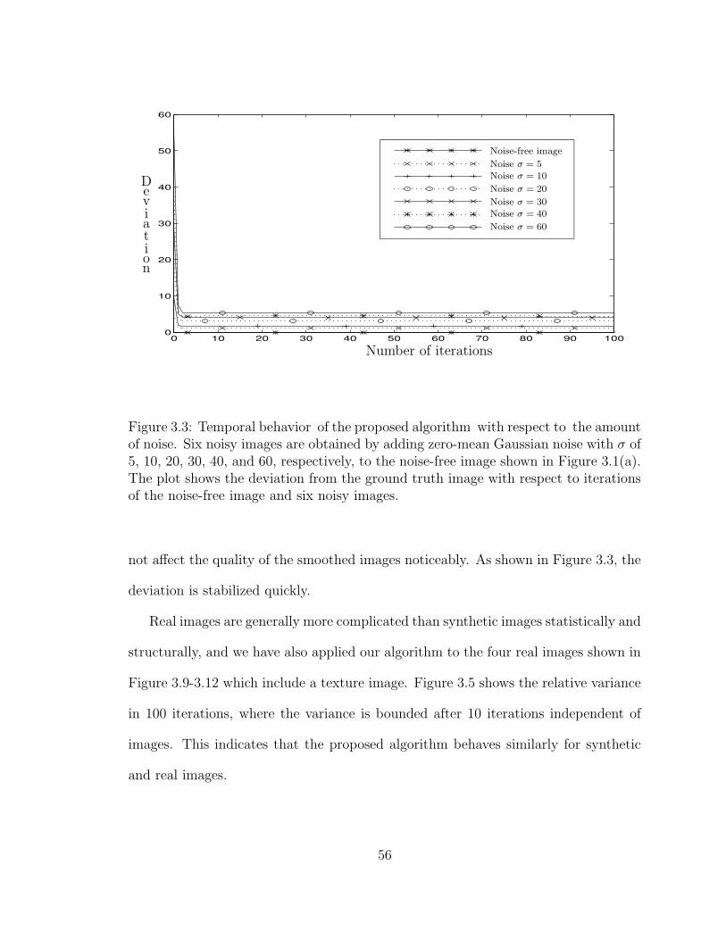
0 10 20 30 40 50 60 70 80 90 1000
10
20
30
40
50
60
Number of iterations
Deviation
Noise-free image
Noise σ = 5
Noise σ = 10
Noise σ = 20
Noise σ = 30Noise σ = 40
Noise σ = 60
Figure 3.3: Temporal behavior of the proposed algorithm with respect to the amountof noise. Six noisy images are obtained by adding zero-mean Gaussian noise with σ of5, 10, 20, 30, 40, and 60, respectively, to the noise-free image shown in Figure 3.1(a).The plot shows the deviation from the ground truth image with respect to iterationsof the noise-free image and six noisy images.
not affect the quality of the smoothed images noticeably. As shown in Figure 3.3, the
deviation is stabilized quickly.
Real images are generally more complicated than synthetic images statistically and
structurally, and we have also applied our algorithm to the four real images shown in
Figure 3.9-3.12 which include a texture image. Figure 3.5 shows the relative variance
in 100 iterations, where the variance is bounded after 10 iterations independent of
images. This indicates that the proposed algorithm behaves similarly for synthetic
and real images.
56
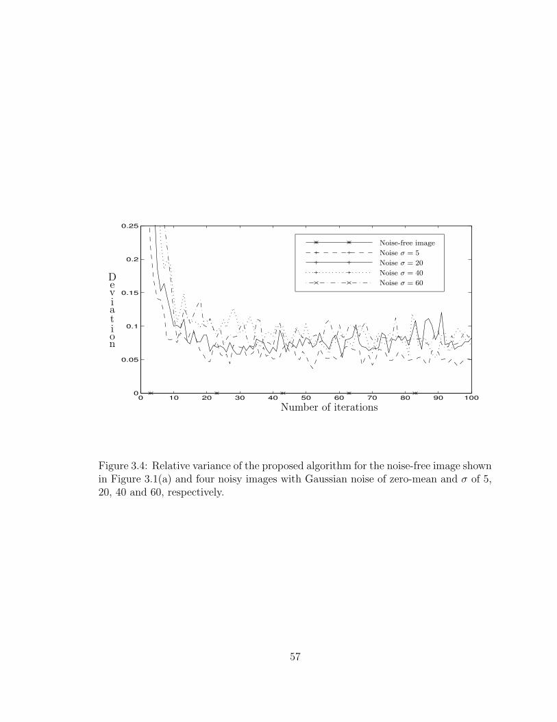
0 10 20 30 40 50 60 70 80 90 1000
0.05
0.1
0.15
0.2
0.25
Number of iterations
Deviation
Noise-free image
Noise σ = 5
Noise σ = 20
Noise σ = 40
Noise σ = 60
Figure 3.4: Relative variance of the proposed algorithm for the noise-free image shownin Figure 3.1(a) and four noisy images with Gaussian noise of zero-mean and σ of 5,20, 40 and 60, respectively.
57
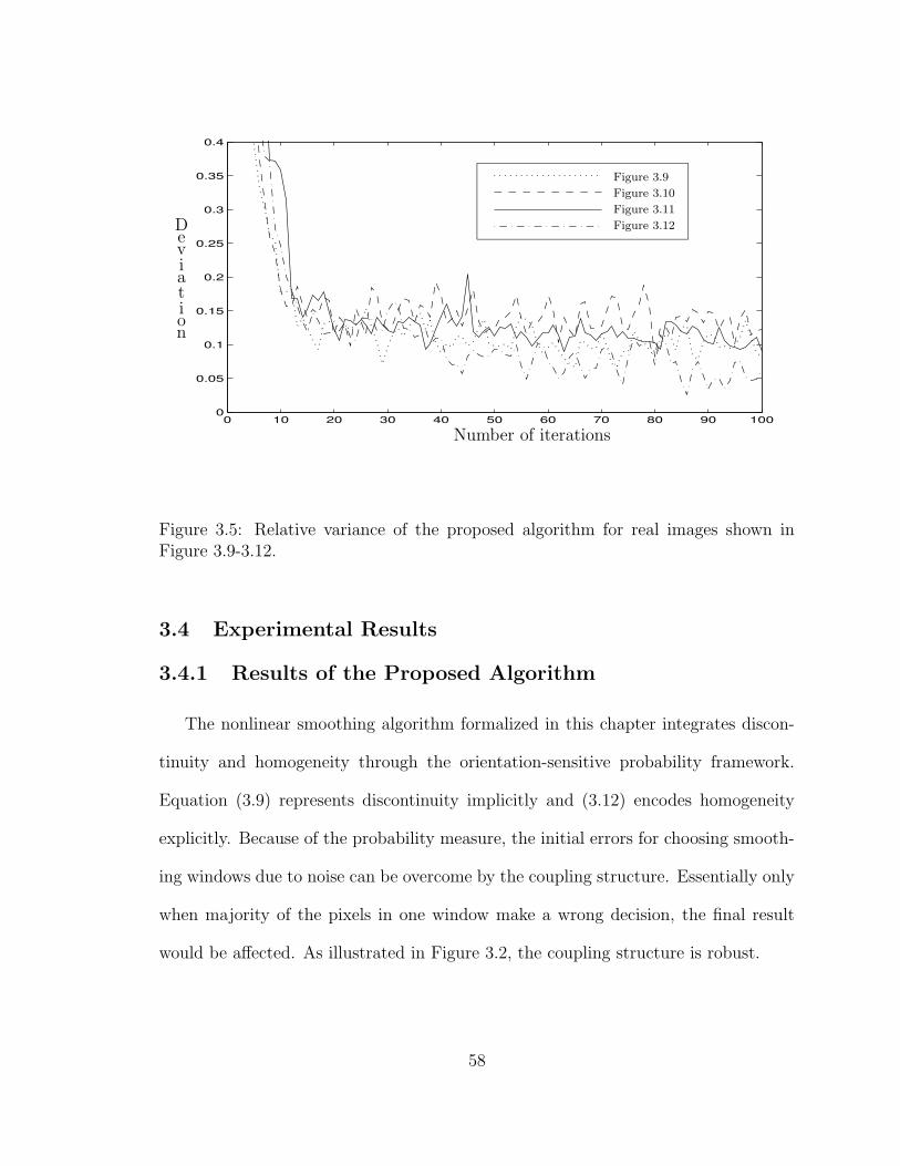
0 10 20 30 40 50 60 70 80 90 1000
0.05
0.1
0.15
0.2
0.25
0.3
0.35
0.4
Number of iterations
Deviation
Figure 3.9
Figure 3.10
Figure 3.11
Figure 3.12
Figure 3.5: Relative variance of the proposed algorithm for real images shown inFigure 3.9-3.12.
3.4 Experimental Results
3.4.1 Results of the Proposed Algorithm
The nonlinear smoothing algorithm formalized in this chapter integrates discon-
tinuity and homogeneity through the orientation-sensitive probability framework.
Equation (3.9) represents discontinuity implicitly and (3.12) encodes homogeneity
explicitly. Because of the probability measure, the initial errors for choosing smooth-
ing windows due to noise can be overcome by the coupling structure. Essentially only
when majority of the pixels in one window make a wrong decision, the final result
would be affected. As illustrated in Figure 3.2, the coupling structure is robust.
58

Figure 3.6: The oriented bar-like windows used throughout this chapter for syntheticand real images. The size of each kernel is approximately 3 x 10 in pixels.
To achieve optimal performance, the size and shape of the oriented windows are
application dependent. However, due to the underlying coupling structure, the pro-
posed algorithm gives good results for a wide range of parameter values. For example,
the same oriented windows are used throughout the experiments in this chapter. As
shown in Figure 3.6, these oriented windows are generated by rotating two rectan-
gular basis windows with size of 3 x 10 in pixels. The preferred orientation of each
window is consistent with orientation sensitivity of cell responses in the visual cortex
[53]. Asymmetric window shapes are used so that 2-D features such as corners and
junctions can be preserved.
As is evident from numerous simulations, the proposed algorithm generates stable
results around 10 iterations regardless of input images. Thus, all the boundaries from
the proposed algorithm are generated using smoothed images at the 11th iteration.
As stated above, boundaries are detected using the Sobel edge detector due to its
efficiency.
Figure 3.7 shows the results by applying the proposed algorithm on a set of noisy
images obtained from the noise-free image shown in Figure 3.1(a) by adding Gaussian
noise with σ of 10, 40, and 60 respectively. Same parameters for smoothing are used
59
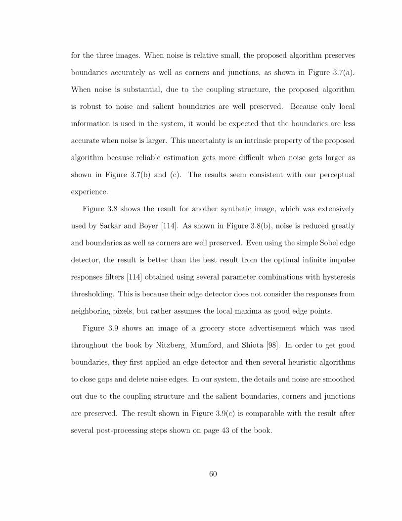
for the three images. When noise is relative small, the proposed algorithm preserves
boundaries accurately as well as corners and junctions, as shown in Figure 3.7(a).
When noise is substantial, due to the coupling structure, the proposed algorithm
is robust to noise and salient boundaries are well preserved. Because only local
information is used in the system, it would be expected that the boundaries are less
accurate when noise is larger. This uncertainty is an intrinsic property of the proposed
algorithm because reliable estimation gets more difficult when noise gets larger as
shown in Figure 3.7(b) and (c). The results seem consistent with our perceptual
experience.
Figure 3.8 shows the result for another synthetic image, which was extensively
used by Sarkar and Boyer [114]. As shown in Figure 3.8(b), noise is reduced greatly
and boundaries as well as corners are well preserved. Even using the simple Sobel edge
detector, the result is better than the best result from the optimal infinite impulse
responses filters [114] obtained using several parameter combinations with hysteresis
thresholding. This is because their edge detector does not consider the responses from
neighboring pixels, but rather assumes the local maxima as good edge points.
Figure 3.9 shows an image of a grocery store advertisement which was used
throughout the book by Nitzberg, Mumford, and Shiota [98]. In order to get good
boundaries, they first applied an edge detector and then several heuristic algorithms
to close gaps and delete noise edges. In our system, the details and noise are smoothed
out due to the coupling structure and the salient boundaries, corners and junctions
are preserved. The result shown in Figure 3.9(c) is comparable with the result after
several post-processing steps shown on page 43 of the book.
60
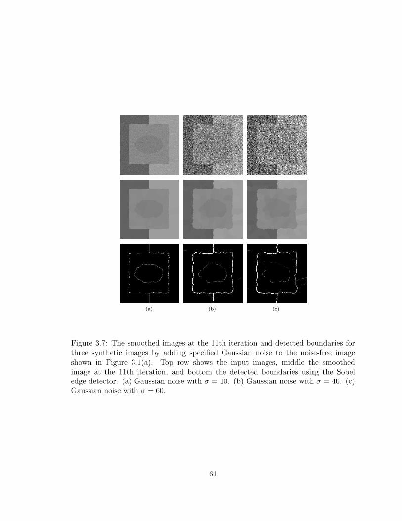
(a) (b) (c)
Figure 3.7: The smoothed images at the 11th iteration and detected boundaries forthree synthetic images by adding specified Gaussian noise to the noise-free imageshown in Figure 3.1(a). Top row shows the input images, middle the smoothedimage at the 11th iteration, and bottom the detected boundaries using the Sobeledge detector. (a) Gaussian noise with σ = 10. (b) Gaussian noise with σ = 40. (c)Gaussian noise with σ = 60.
61
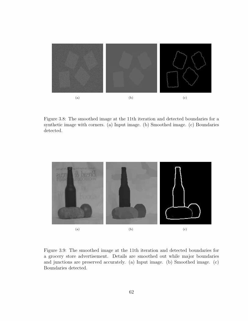
(a) (b) (c)
Figure 3.8: The smoothed image at the 11th iteration and detected boundaries for asynthetic image with corners. (a) Input image. (b) Smoothed image. (c) Boundariesdetected.
(a) (b) (c)
Figure 3.9: The smoothed image at the 11th iteration and detected boundaries fora grocery store advertisement. Details are smoothed out while major boundariesand junctions are preserved accurately. (a) Input image. (b) Smoothed image. (c)Boundaries detected.
62

(a) (b) (c)
Figure 3.10: The smoothed image at the 11th iteration and detected boundaries fora natural satellite image with several land use patterns. The boundaries betweendifferent regions are formed from noisy segments due to the coupling structure. (a)Input image. (b) Smoothed image. (c) Boundaries detected.
Figure 3.10 shows a high resolution satellite image of a natural scene, consisting of
a river, soil land, and a forest. As shown in Figure 3.10(b), the river boundary which
is partially occluded by the forest is delineated. The textured forest is smoothed out
into a homogeneous region. The major boundaries between different types of features
are detected correctly.
Figure 3.11 shows an image of a woman which includes detail features and shading
effects, the color version of which was used by Zhu and Yuille [151]. In their region
competition algorithm, Zhu and Yuille [151] used a mixture of Gaussian model. A
non-convex energy function consisting of several constraint terms was formulated
under Bayesian framework. The algorithm, derived using variational principles, is
guaranteed to converge to only a local minimum. For our nonlinear algorithm, as
shown in Figure 3.11(b), the details are smoothed out while important boundaries
are preserved. The final result in Figure 3.11(c) is comparable with the result from the
region competition algorithm [151] applied on the color version after 130 iterations.
Compared with the region competition algorithm, the main advantage of our approach
63
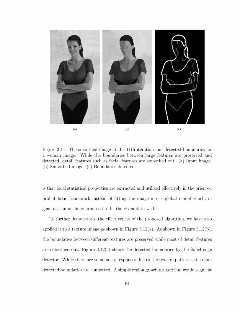
(a) (b) (c)
Figure 3.11: The smoothed image at the 11th iteration and detected boundaries fora woman image. While the boundaries between large features are preserved anddetected, detail features such as facial features are smoothed out. (a) Input image.(b) Smoothed image. (c) Boundaries detected.
is that local statistical properties are extracted and utilized effectively in the oriented
probabilistic framework instead of fitting the image into a global model which, in
general, cannot be guaranteed to fit the given data well.
To further demonstrate the effectiveness of the proposed algorithm, we have also
applied it to a texture image as shown in Figure 3.12(a). As shown in Figure 3.12(b),
the boundaries between different textures are preserved while most of detail features
are smoothed out. Figure 3.12(c) shows the detected boundaries by the Sobel edge
detector. While there are some noisy responses due to the texture patterns, the main
detected boundaries are connected. A simple region growing algorithm would segment
64
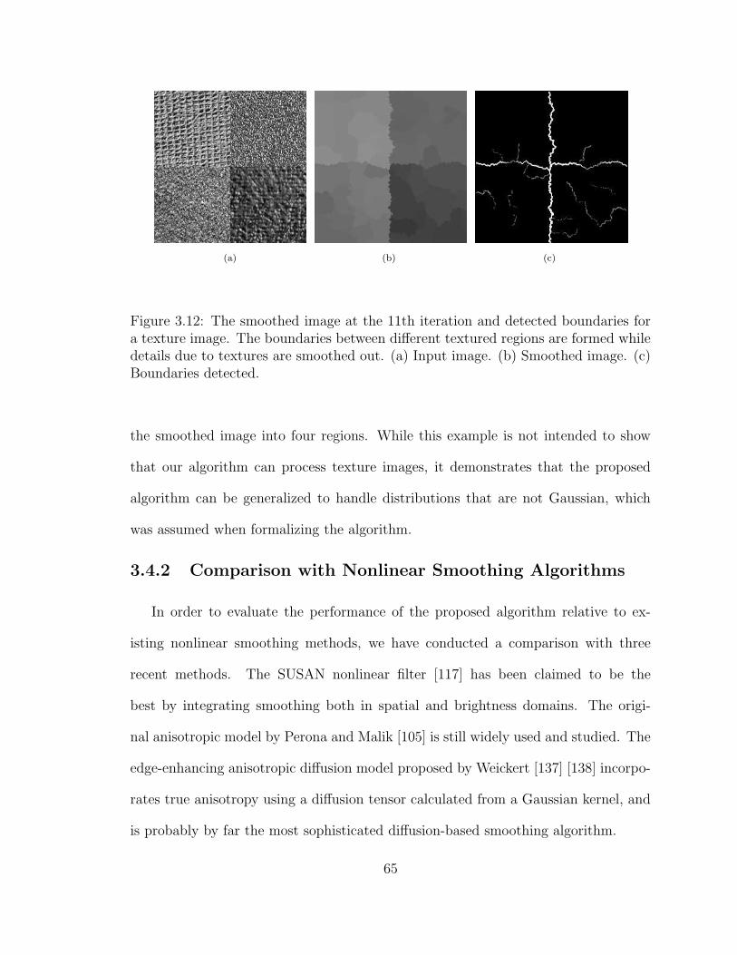
(a) (b) (c)
Figure 3.12: The smoothed image at the 11th iteration and detected boundaries fora texture image. The boundaries between different textured regions are formed whiledetails due to textures are smoothed out. (a) Input image. (b) Smoothed image. (c)Boundaries detected.
the smoothed image into four regions. While this example is not intended to show
that our algorithm can process texture images, it demonstrates that the proposed
algorithm can be generalized to handle distributions that are not Gaussian, which
was assumed when formalizing the algorithm.
3.4.2 Comparison with Nonlinear Smoothing Algorithms
In order to evaluate the performance of the proposed algorithm relative to ex-
isting nonlinear smoothing methods, we have conducted a comparison with three
recent methods. The SUSAN nonlinear filter [117] has been claimed to be the
best by integrating smoothing both in spatial and brightness domains. The origi-
nal anisotropic model by Perona and Malik [105] is still widely used and studied. The
edge-enhancing anisotropic diffusion model proposed by Weickert [137] [138] incorpo-
rates true anisotropy using a diffusion tensor calculated from a Gaussian kernel, and
is probably by far the most sophisticated diffusion-based smoothing algorithm.
65
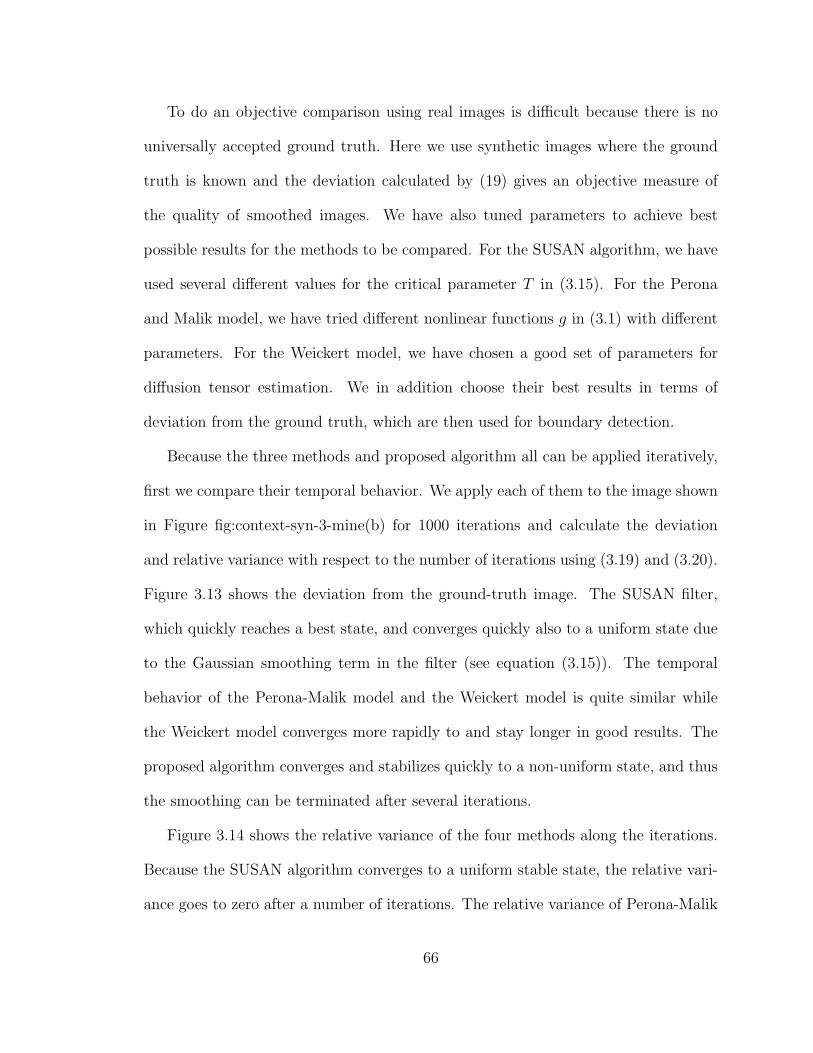
To do an objective comparison using real images is difficult because there is no
universally accepted ground truth. Here we use synthetic images where the ground
truth is known and the deviation calculated by (19) gives an objective measure of
the quality of smoothed images. We have also tuned parameters to achieve best
possible results for the methods to be compared. For the SUSAN algorithm, we have
used several different values for the critical parameter T in (3.15). For the Perona
and Malik model, we have tried different nonlinear functions g in (3.1) with different
parameters. For the Weickert model, we have chosen a good set of parameters for
diffusion tensor estimation. We in addition choose their best results in terms of
deviation from the ground truth, which are then used for boundary detection.
Because the three methods and proposed algorithm all can be applied iteratively,
first we compare their temporal behavior. We apply each of them to the image shown
in Figure fig:context-syn-3-mine(b) for 1000 iterations and calculate the deviation
and relative variance with respect to the number of iterations using (3.19) and (3.20).
Figure 3.13 shows the deviation from the ground-truth image. The SUSAN filter,
which quickly reaches a best state, and converges quickly also to a uniform state due
to the Gaussian smoothing term in the filter (see equation (3.15)). The temporal
behavior of the Perona-Malik model and the Weickert model is quite similar while
the Weickert model converges more rapidly to and stay longer in good results. The
proposed algorithm converges and stabilizes quickly to a non-uniform state, and thus
the smoothing can be terminated after several iterations.
Figure 3.14 shows the relative variance of the four methods along the iterations.
Because the SUSAN algorithm converges to a uniform stable state, the relative vari-
ance goes to zero after a number of iterations. The relative variance of Perona-Malik
66
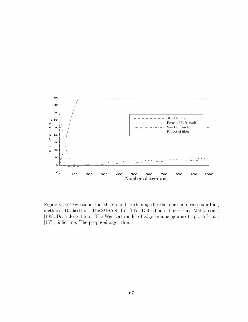
0 100 200 300 400 500 600 700 800 900 10000
5
10
15
20
25
30
35
40
45
50
Number of iterations
Deviation
SUSAN filter
Perona-Malik model
Weickert model
Proposed filter
Figure 3.13: Deviations from the ground truth image for the four nonlinear smoothingmethods. Dashed line: The SUSAN filter [117]; Dotted line: The Perona-Malik model[105]; Dash-dotted line: The Weickert model of edge enhancing anisotropic diffusion[137]; Solid line: The proposed algorithm.
67

0 100 200 300 400 500 600 700 800 900 10000
0.5
1
1.5
2
2.5
Number of iterations
Deviation
SUSAN filter
Perona-Malik model
Weickert model
Proposed filter
Figure 3.14: Relative variance of the four nonlinear smoothing methods. Dashedline: The SUSAN filter [117]; Dotted line: The Perona-Malik diffusion model [105];Dash-dotted line: The Weickert model [137]; Solid line: The proposed algorithm.
model is closely related to the g function in (3.1). Due to the spatial regularization
using a Gaussian kernel, Weickert model changes continuously and the diffusion lasts
much longer, which accounts for the fact why good results exist for a longer period
of time than Perona-Malik model. As shown in Figure 3.4 and 3.5, the proposed
algorithm generates bounded small ripples in the relative variance measure. Those
ripples do not affect smoothing results noticeably as the deviation from the ground
truth, shown in Figure 3.13, is stabilized quickly.
Now we compare the effectiveness of the four methods in preserving meaningful
boundaries. Following Higgins and Hsu [47], we use two quantitative performance
metrics to compare the edge detection results: P (AE|TE), the probability of a true
68
edge pixel being correctly detected by a given method; P (TE|AE), the probability
of a detected edge pixel being a true edge pixel. Due to the uncertainty in edge
localization, a detected edge pixel is considered to be correct if it is within two pixels
from ground-truth edge points using the noise-free image. For each method, the
threshold on the gradient magnitude of the Sobel edge detector is adjusted to achieve
a best trade-off between detecting true edge points and rejecting false edge points.
For the proposed algorithm, we use the result at the 11th iteration because the
proposed algorithm converges within several iterations. As mentioned before, for the
other three methods, we tune critical parameters and choose the smoothed images
with the smallest deviation. Figure 3.15 shows the smoothed images along with the
detected boundaries using the Sobel edge detector, for the image shown in Figure
fig:context-syn-3-mine(a), where added noise is Gaussian with zero mean and σ = 10.
Table 3.1 summarizes the quantitative performance metrics. All of the four methods
perform well and the proposed method gives the best numerical scores. The boundary
of the square is preserved accurately. For the central oval, the proposed algorithm
gives a better connected boundary while the other three have gaps. Also the proposed
algorithm generated the sharpest edges while edges from Weickert model are blurred
most, resulting in the worst numerical metrics among the four methods.
Figure 3.16 shows the result for the image in Figure 3.7(b), where noise is sub-
stantial, and Table 3.2 shows the quantitative performance metrics. As shown in
Figure 3.16(a), the SUSAN filter tends to fail to preserve boundaries, resulting in
noisy boundary fragments. The Perona-Malik model produces good but fragmented
boundaries. Due to that only local gradient is used, the Perona-Malik model is noise-
sensitive and thus generates more false responses than other methods in this case.
69

(a) (b) (c) (d)
Figure 3.15: Smoothing results and detected boundaries of the four nonlinear methodsfor a synthetic image shown in Figure 3.7(a). Here noise is not large and all of themethods perform well in preserving boundaries.
The false responses substantially lower the quantitative metrics of the model, making
it the worst among the four methods. The Weickert model produces good bound-
aries for strong segments but weak segments are blurred considerably. The proposed
algorithm preserves the connected boundary of the square and partially fragmented
boundaries of the central oval also, yielding the best numerical metrics among the four
methods. As shown in Figure 3.13, the smoothed image of the Weickert model has a
smaller deviation than the result from our algorithm, but the detected boundaries are
fragmented. This is because our algorithm produces sharp boundaries, which induce
larger penalties according to (3.19) when not accurately marked.
Comparing Tables 3.1 and 3.2, one can see that our proposed method is most
robust in that the average performance is degraded by about 13%. Perona-Malik
model is most noise-sensitive, where the performance is degraded by about 35%. For
70

Models SUSAN[117] Perona-Malik[105] Weickert[137][138] Our method
P (TE | AE) 0.960 0.963 0.877 0.988
P (AE | TE) 0.956 0.964 0.880 0.979
Average 0.958 0.963 0.878 0.983
Table 3.1: Quantitative comparison of boundary detection results shown in Figure3.15.
Models SUSAN[117] Perona-Malik[105] Weickert[137][138] Our method
P (TE | AE) 0.720 0.609 0.692 0.853
P (AE | TE) 0.713 0.618 0.688 0.854
Average 0.717 0.613 0.690 0.853
Table 3.2: Quantitative comparison of boundary detection results shown in Figure3.16.
SUSAN and Weickert model, the average performance is degraded by about 24% and
19% respectively.
We have also applied the four methods on the natural satellite image shown in
Figure 3.10. The result from the proposed algorithm is at the 11th iteration as
already shown in Figure 3.10. The results from the other three methods are picked up
manually for best possible results. Due to the termination problem, results from most
nonlinear smoothing algorithms have to be chosen manually, making them difficult
to be used automatically. The results from the other three methods are similar,
and boundaries between different regions are not formed. In contrast, our algorithm
generated connected boundaries separating major different regions.
71
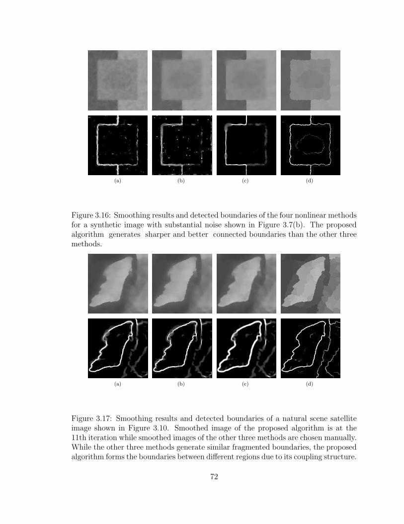
(a) (b) (c) (d)
Figure 3.16: Smoothing results and detected boundaries of the four nonlinear methodsfor a synthetic image with substantial noise shown in Figure 3.7(b). The proposedalgorithm generates sharper and better connected boundaries than the other threemethods.
(a) (b) (c) (d)
Figure 3.17: Smoothing results and detected boundaries of a natural scene satelliteimage shown in Figure 3.10. Smoothed image of the proposed algorithm is at the11th iteration while smoothed images of the other three methods are chosen manually.While the other three methods generate similar fragmented boundaries, the proposedalgorithm forms the boundaries between different regions due to its coupling structure.
72

3.5 Conclusions
In this chapter we have presented a two-step robust boundary detection algo-
rithm. The first step is a nonlinear smoothing algorithm based on an orientation
sensitive probability measure. This algorithm is motivated by the orientation sen-
sitivity of cells in the visual cortex [53]. By incorporating geometrical constraints
through the coupling structure, the algorithm is robust to noise while preserving
meaningful boundaries. Even though the algorithm was formulated based on Gaus-
sian distribution, it performs well for real and even textured images, showing the
generalization capability of the algorithm. It is also easy to see that the formalization
of the proposed algorithm would extend to other known distribution by changing
equations (3.3)-(3.5) accordingly. One such an extension would be to use a mixture
of Gaussian distributions [30] so that the model may be able to describe arbitrary
probability distribution.
Compared with recent anisotropic diffusion methods, our algorithm approaches a
non-uniform stable state and reliable results can be obtained after a fixed number of
iterations. In other words, it provides a solution for the termination problem. When
noise is substantial, our algorithm preserves meaningful boundaries better than the
diffusion-based methods, because the coupling structure employed is more robust
than pair-wise coupling structure.
Scale is an intrinsic parameter in machine vision as interesting features may exist
only in a limited range of scales. Scale spaces based on linear and nonlinear smooth-
ing kernels do not represent semantically meaningful structures explicitly [122]. A
solution to the problem could be to use parameter K in equation (3.8) as a control
73

parameter [113], which is essentially a threshold in gray values. Under this formal-
ization, (3.12) could offer an adaptive parameter selection. With the robust coupling
structure, our algorithm with adaptive parameter selection may be able to provide a
robust multiscale boundary detection method.
Another advantage of the probability measure framework is that there is no need
to assume a priori knowledge about each region, which is necessary in relaxation
labeling [112] [55] and the comparison across windows with different sizes and shapes
is feasible. This could lead to an adaptive window selection that preserves small but
important features which cannot be handled well by the current implementation.
There is one intrinsic limitation common to many smoothing approaches including
our proposed one. After smoothing, the available feature is the average gray value,
resulting in loss of information for further processing. One way to overcome this
problem is to apply the smoothing in feature spaces derived from input images [139].
Another disadvantage of the proposed algorithm is relatively intensive computation
due to the use of oriented windows. Each oriented window takes roughly as long
in one iteration as the edge-enhancing diffusion method [137]. On the other hand,
because our algorithm is entirely local and parallel, computation time would not be
a problem on parallel and distributed hardware. Computation on serial computers
could be reduced dramatically by decomposing the oriented filters hierarchically so
that oriented windows would be used only around discontinuities rather than in ho-
mogeneous regions. The decomposition techniques for steerable and scalable filters
[104] could also help to reduce the number of necessary convolution kernels.
74

CHAPTER 4
SPECTRAL HISTOGRAM: A GENERIC FEATURE FOR
IMAGES
In this chapter, we propose a generic statistic feature for homogeneous texture im-
ages, which we call spectral histograms. A similarity measure between any given image
patches is then defined as the Kullback-Leibler divergence or other distance measures
between the corresponding spectral histograms. Unlike other similarity measures,
it can discriminate texture as well as intensity images and provide a unified, non-
parametric similarity measure for images. We demonstrate this using examples in
texture image synthesis [147], texture image classification, and content-based image
retrieval. We compare several different distance measures and find that the spectral
histogram is not sensitive to the particular form of distance measure. We also com-
pare the spectral histogram with other statistic features and find that the spectral
histogram gives the best result for classification of a texture image database. We find
that distribution of local features is important while the local features themselves do
not appear to be critically important for texture discrimination and classification.
75

4.1 Introduction
As discussed in Chapter 1, the ultimate goal of a machine vision system is to
derive a description of input images. To build an efficient and effective machine vision
system, a critical step is to derive meaningful features. Here “meaningful” states that
the high-level modules such as recognition should be able to use the derived features
readily. To illustrate the problem, Figure 1.1(a) shows a texture image and a small
patch from 1.1(a) is shown in Figure 1.1(b). Figure 1.1(c) shows the numerical values
of (b). It is extremely difficult, if not impossible, to derive a segmentation or useful
representation for the given image purely based on the numerical values. This example
demonstrates that features need to be extracted based on input images for machine
vision systems as well as for biological vision systems.
While many algorithms and systems have been proposed for image segmentation,
classification, and recognition, feature extraction is not well addressed. In most cases,
features are chosen by assumption for mathematical convenience or domain-specific
heuristics. For example, Canny [13] derived the most widely used edge detection
algorithm based on a step edge with additive Gaussian noise. Using variational tech-
niques, he obtained the optimal filter for the assumed model and proposed the first-
order derivative of Gaussian as an efficient and good approximation. Inspired by
the neurophysiological experimental findings of on- and off-center simple cells [54]
[53], Marr and Hildreth [89] proposed the second-order derivative of Gaussian (LoG,
Laplacian of Gaussian) to model the responses of the on- and off-center cells. This
simple, piece-wise constant model has been widely used in image segmentation al-
gorithms. For example, Mumford and Shah [94] proposed an energy functional for
76
image segmentation
E(f,Γ) = µ∫ ∫
R(f − I)2dxdy +
∫ ∫
R\Γ‖ ∇f ‖2 dxdy + ν|Γ|. (4.1)
Here I is a two-dimensional input image defined on R, and f is the solution to be
found and Γ is the boundary of f . One can see that the underlying assumption of
the solution space is piece-wise smooth images. The energy functional shown in (4.1)
was claimed to be a generic energy functional [92] in that most existing segmentation
algorithms and techniques can be derived from the proposed energy functional.
Another major line of research related to feature extraction is texture discrimina-
tion and classification/segmentation. There are no obvious features that work well
for all texture images. The human visual system, however, can discriminate textures
robustly and effectively. This observation inspired many research activities. Julesz
[62] pioneered the research in searching for feature statistics for human visual per-
ception. He first studied k-gon statistics and conjectured that k = 2 is sufficient for
human visual perception. The conjecture was experimentally disproved by synthesiz-
ing perceptually different textures with identical 2-gon statistics [11] [24]. Other early
features for texture discrimination include co-occurrence matrices [44] [43], first-order
statistics [61], second-order statistics [18], and Markov random fields [65] [21] [16].
Those features have limited expressive power due to that the analysis of spatial inter-
action is limited to a relatively small neighborhood [147] and are applied successfully
to so-called micro-textures.
In the 1980s, theories on human texture perception were established, largely
based on available psychophysical and neurophysiological data [12] [23] and joint
spatial/frequency representation. Theories state that the human visual system trans-
forms the retinal image into local spatial/frequency representation, which can be
77

computationally simulated by convolving the input image with a bank of filters with
tuned frequencies and orientations. The mathematical framework for the local spa-
tial/frequency was laid out by Gabor [33] in the context of communication systems.
In Fourier transform, a signal can be represented in time and frequency domains. The
basis functions in time domain are impulses with different time delays, and the basis
functions in frequency domain are complex sinusoid functions with different frequen-
cies. A major problem with Fourier transform is localization. As shown in Figure
4.1, while the impulse in time domain precisely localizes the signal component, its
Fourier transform does not provide any localization information in frequency domain.
While the sinusoid function provides accurate localization in frequency domain, it
is not possible to localize the signal in time domain. Essentially, Fourier transform
uses two basis functions, which provides best localization in one domain and no lo-
calization in the other. Based on this observation, Gabor proposed a more generic
time/frequency representation [33], where the basis functions of Fourier transforms
are just two opposite extremes. By minimizing the localization uncertainty both in
time and frequency domains, Gabor proposed basis functions, which can achieve the
optimality simultaneously in time and frequency domains. Gabor basis functions were
extended to two-dimensional images by Daugman [22]. Very recently, this theory has
also been confirmed by deriving similar feature detectors from natural images based
on certain optimization criteria [100] [101] [102] [1].
The human perception theory and the local spatial/frequency representational
framework inspired much research in texture classification and segmentation. Within
this framework, however, statistic features still need to be chosen due to that filter
78
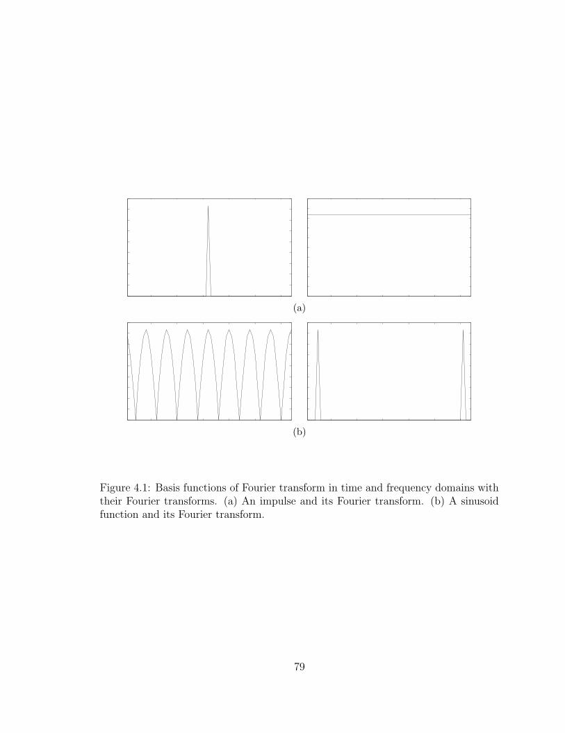
(a)
(b)
Figure 4.1: Basis functions of Fourier transform in time and frequency domains withtheir Fourier transforms. (a) An impulse and its Fourier transform. (b) A sinusoidfunction and its Fourier transform.
79
responses are not homogeneous within homogeneous textures and not sufficient be-
cause they are linear. As shown in Figure 4.2, a Gabor filter, shown in Figure 4.2(b),
responses to local and oriented structures, as shown in Figure 4.2(c), and the filter
response itself does not characterize the texture. Intuitively, texture appearance can
not be characterized by very local pixel values because texture is a regional prop-
erty. If we want to define a feature that is homogeneous within a texture region, it
is necessary to integrate responses from filters with multiple orientations and scales.
In other words, features need to be defined as statistic measures on filter responses.
For example, Unser [127] used variances from different filters to characterize textures.
Ojala et al [99] compared different features for texture classification using the distri-
bution of detected local features using a database consisting of nine images. Puzicha
et al [107] used a distribution of responses from a set of Gabor filters as features.
However, they posed the texture segmentation as an energy minimization based on a
pair-wise discrimination matrix, and the features used are not analyzed in terms of
characterizing texture appearance.
Recently, Heeger and Bergen [45] proposed a texture synthesis algorithm that can
match texture appearance. The algorithm tries to transform a random noisy image
into an image with similar appearance to the given target image by matching inde-
pendently the histograms of image pyramids constructed from the noisy and target
images. The experimental results are impressive even though no theoretical justifi-
cation was given. De Bonet and Viola [8] attempted to match the joint histograms
by utilizing the conditional probability defined on parent vectors. A parent vector is
a vector consisting of the filter responses in the constructed image pyramid up to a
80
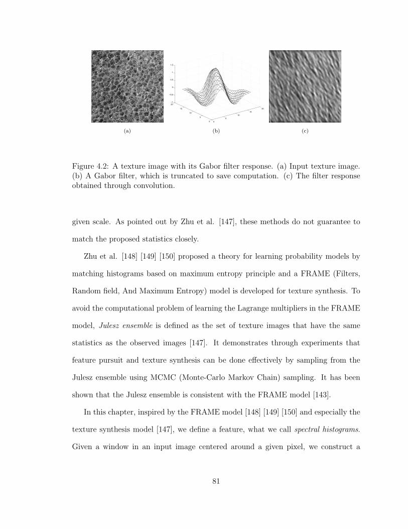
0
5
10
15
20
0
5
10
15
20−1
−0.5
0
0.5
1
1.5
(a) (b) (c)
Figure 4.2: A texture image with its Gabor filter response. (a) Input texture image.(b) A Gabor filter, which is truncated to save computation. (c) The filter responseobtained through convolution.
given scale. As pointed out by Zhu et al. [147], these methods do not guarantee to
match the proposed statistics closely.
Zhu et al. [148] [149] [150] proposed a theory for learning probability models by
matching histograms based on maximum entropy principle and a FRAME (Filters,
Random field, And Maximum Entropy) model is developed for texture synthesis. To
avoid the computational problem of learning the Lagrange multipliers in the FRAME
model, Julesz ensemble is defined as the set of texture images that have the same
statistics as the observed images [147]. It demonstrates through experiments that
feature pursuit and texture synthesis can be done effectively by sampling from the
Julesz ensemble using MCMC (Monte-Carlo Markov Chain) sampling. It has been
shown that the Julesz ensemble is consistent with the FRAME model [143].
In this chapter, inspired by the FRAME model [148] [149] [150] and especially the
texture synthesis model [147], we define a feature, what we call spectral histograms.
Given a window in an input image centered around a given pixel, we construct a
81

pyramid based on the local window using a bank of chosen filters. We calculate the
histogram for each local window in the pyramid. We obtain a vector, consisting of
the histograms from all filters, which is defined as spectral histogram at the given
location.
For chosen statistic features to be used for successive modules, such as classifica-
tion, segmentation, and recognition, a similarity/distance measure must be defined.
A distance measure between two spectral histograms is defined as the χ2-statistic or
other distance measures between the spectral histograms. A distance measure using
χ2-statistic was proposed based on empirical experiments [107] [50]. However, as we
will demonstrate using classification, the particular form of distance measure is not
critical for spectral histograms.
In Section 4.2, we formally define spectral histograms and give some properties
of spectral histograms. In Section 4.3 we show how to synthesize texture images
by matching spectral histograms. In Section 4.4, we study spectral histograms for
texture classification. In Section 4.5, we apply spectral histograms to the problem of
content-based image retrieval. In Section 4.6, we compare different texture features
and different similarity measures using classification. In Section 4.7, we apply our
model to synthetic texture pair discrimination. Section 4.8 concludes this chapter
with further discussion.
4.2 Spectral Histograms
Given an input image I, defined on a finite two-dimensional lattice, and a bank
of filters F (α), α = 1, 2, . . . , K, a sub-band image I(α) is computed for each filter
through linear convolution, i.e., I(α)(v) = F (α) ∗ I(v) =∑
u F (u)I(v − u). I(α), α =
82

1, 2, . . . , K can be considered as an image pyramid constructed from the given image
I when there exist scaling relationships among the chosen filters. Here we loosely call
I(α), α = 1, 2, . . . , K as an image pyramid for an arbitrary chosen bank of filters. For
each sub-band image, we define the marginal distribution, or histogram
H(α)I (z) =
1
|I|∑
v
δ(z − I(α)(v)). (4.2)
We then define the spectral histogram with respect to the chosen filters as
HI = (H(1)I , H
(2)I , . . . , H
(K)I ). (4.3)
Spectral histograms of an image or an image patch are essentially a vector con-
sisting of marginal distributions of filter responses. The size of the input image or
the input image patch is called integration scale. We define a similarity measure be-
tween two spectral histograms using different standard distance measures. Lp-norm
distance is defined as
|HI1 −HI2|p =K∑
α=1
(
∑
z
(H(α)I1
(z)−H(α)I2
(z))p
)(1/p)
. (4.4)
Also because marginal distribution of each filter response is a distribution, a dis-
tance can be defined based on discrete Kullback-Leibler divergence [70]
KL(HI1 , HI2) =K∑
α=1
∑
z
(H(α)I1
(z)−H(α)I2
(z)) logH
(α)I1
(z)
H(α)I2
(z). (4.5)
Another choice for distance is χ2-statistic, which is a first-order approximation of
Kullback-Leibler divergence and is used widely to compare histograms
χ2(HI1 , HI2) =K∑
α=1
∑
z
(H(α)I1
(z)−H(α)I2
(z))2
H(α)I1
(z) +H(α)I2
(z). (4.6)
83

0
5
10
15
20
0
5
10
15
20−1
−0.5
0
0.5
1
1.5
(a) (b) (c)
(d)
Figure 4.3: A texture image and its spectral histograms. (a) Input image. (b) AGabor filter. (c) The histogram of the filter. (d) Spectral histograms of the image.There are eight filters including intensity filter, gradient filters Dxx and Dyy, fourLoG filters with T =
√2/2, 1, 2, and 4, and a Gabor filter Gcos(12, 150). There
are 8 bins in the histograms of intensity and gradient filters and 11 bins for the otherfilters.
84
4.2.1 Properties of Spectral Histograms
Images sharing the same spectral histograms define an ensemble, called Julesz
ensemble [147]. Equivalence between Julesz ensemble and the FRAME model [149]
[150] has been established [143].
As proven in [150], the true probability model of one type of texture images can
be approximated by linear combinations of marginal distributions given in spectral
histograms. In other words, spectral histograms provide a set of “basis functions” for
statistic modeling of texture images.
The spectral histogram and the associated distance measure provide a unified
similarity measure for images. Because the marginal distribution is independent of
image sizes, any two image patches can be compared using the spectral histogram.
Naturally, we can define a scale space using different integration scales, which can be
used to measure the homogeneity. This will be studied in the next chapter.
Due to that spectral histograms are based on marginal distributions, they pro-
vide a statistical measure and two images do not need to be aligned in order to be
compared.
4.2.2 Choice of Filters
The filters used consist of filters that are consistent with the human perception
theory. Following Zhu et al [149], we use four kinds of filters.
1. The intensity filter, which is the δ() function and captures the intensity value
at a given pixel.
2. Difference or gradient filters. We use four of them:
85
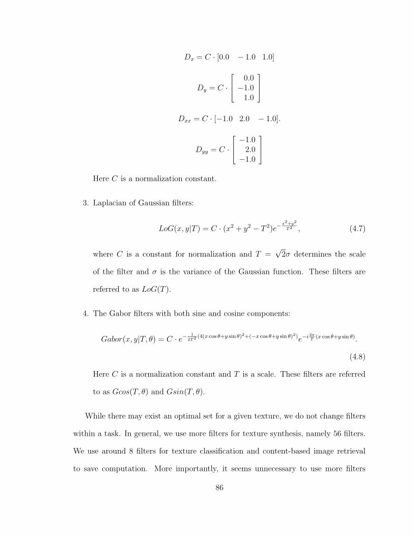
Dx = C · [0.0 − 1.0 1.0]
Dy = C ·
0.0−1.0
1.0
Dxx = C · [−1.0 2.0 − 1.0].
Dyy = C ·
−1.02.0−1.0
Here C is a normalization constant.
3. Laplacian of Gaussian filters:
LoG(x, y|T ) = C · (x2 + y2 − T 2)e−x2+y2
T2 , (4.7)
where C is a constant for normalization and T =√
2σ determines the scale
of the filter and σ is the variance of the Gaussian function. These filters are
referred to as LoG(T ).
4. The Gabor filters with both sine and cosine components:
Gabor(x, y|T, θ) = C · e− 12T2 (4(x cos θ+y sin θ)2+(−x cos θ+y sin θ)2)e−i 2π
T(x cos θ+y sin θ).
(4.8)
Here C is a normalization constant and T is a scale. These filters are referred
to as Gcos(T, θ) and Gsin(T, θ).
While there may exist an optimal set for a given texture, we do not change filters
within a task. In general, we use more filters for texture synthesis, namely 56 filters.
We use around 8 filters for texture classification and content-based image retrieval
to save computation. More importantly, it seems unnecessary to use more filters
86
for texture classification and content-based image retrieval when relatively a small
integration scale is used.
4.3 Texture Synthesis
In this section we demonstrate the effectiveness of the spectral histogram in charac-
terizing texture appearance using texture synthesis. We define a relationship between
two texture images using the divergence between their spectral histograms. There ex-
ists such a relationship if and only if their spectral histograms are sufficiently close.
It is easy to check that this defines an equivalence class.
Given observed feature statistics, H (α)obs , α = 1, ..., K, which are spectral his-
tograms computed from observed images, we define an energy function [147]
E(I) =K∑
α=1
D(H(α)(I) , H
(α)obs). (4.9)
Then the corresponding Gibbs distribution is
q(I) =1
ZΘ
exp(−E(I)Θ
) (4.10)
where Θ is the temperature.
The Gibbs distribution can be sampled by a Gibbs sampler or other MCMC
algorithms. Here we use a Gibbs sampler [147] given in Figure 4.4. In Figure 4.4,
q(Isyn(v) | Isyn(−v)) is the conditional probability of pixel values at v given the rest
of the image. D is a distance measure and L1-norm is used for texture synthesis.
For texture synthesis, we use 56 filters:
• The intensity filter.
• 4 gradient filters.
87

Gibbs Sampler
Compute H(α)obs , α = 1, ..., K from observed texture images.
Initialize Isyn as any image (e.g., white noise).Θ← Θ0.Repeat
Randomly pick up a pixel location v in Isyn.Calculate q(Isyn(v) | Isyn(−v)).Randomly flip one pixel Isyn(v) under q(Isyn(v) | Isyn(−v)).Reduce Θ gradually.
Until D(H(α)(Isyn), H
(α)obs) ≤ ε for α = 1, 2, ..., K.
Figure 4.4: Gibbs sampler for texture synthesis.
• 7 LoG filters with T =√
2/2, 1, 2, 3, 4, 5, and 6.
• 36 Cosine Gabor filters with T = 2, 4, 6, 8, 10, and 12, and six orientations θ
= 0, 30, 60, 90, 120, and 150 at each scale.
• 6 Sine Gabor filters with T = 2, 4, 6, 8, 10, and 12, and one orientation θ =
45 at each scale.
• 2 Sine Gabor filters with T = 2, and 12 and one orientation θ = 60.
Those filters are chosen primarily because they are used by Zhu et al [149]. The
cooling schedule is fixed for all the experiments shown in this section.
Figure 4.5(a) shows a texture image. Figure 4.5(b) shows a white noise image,
which is used as the initial image. After 14 sweeps, the noise image is transformed
gradually to the image shown in Figure 4.5(c) by matching the spectral histogram of
the two images. Figure 4.5(d) shows the L1-norm distance between the spectral his-
togram of the observed and synthesized image with respect to the number of sweeps.
88
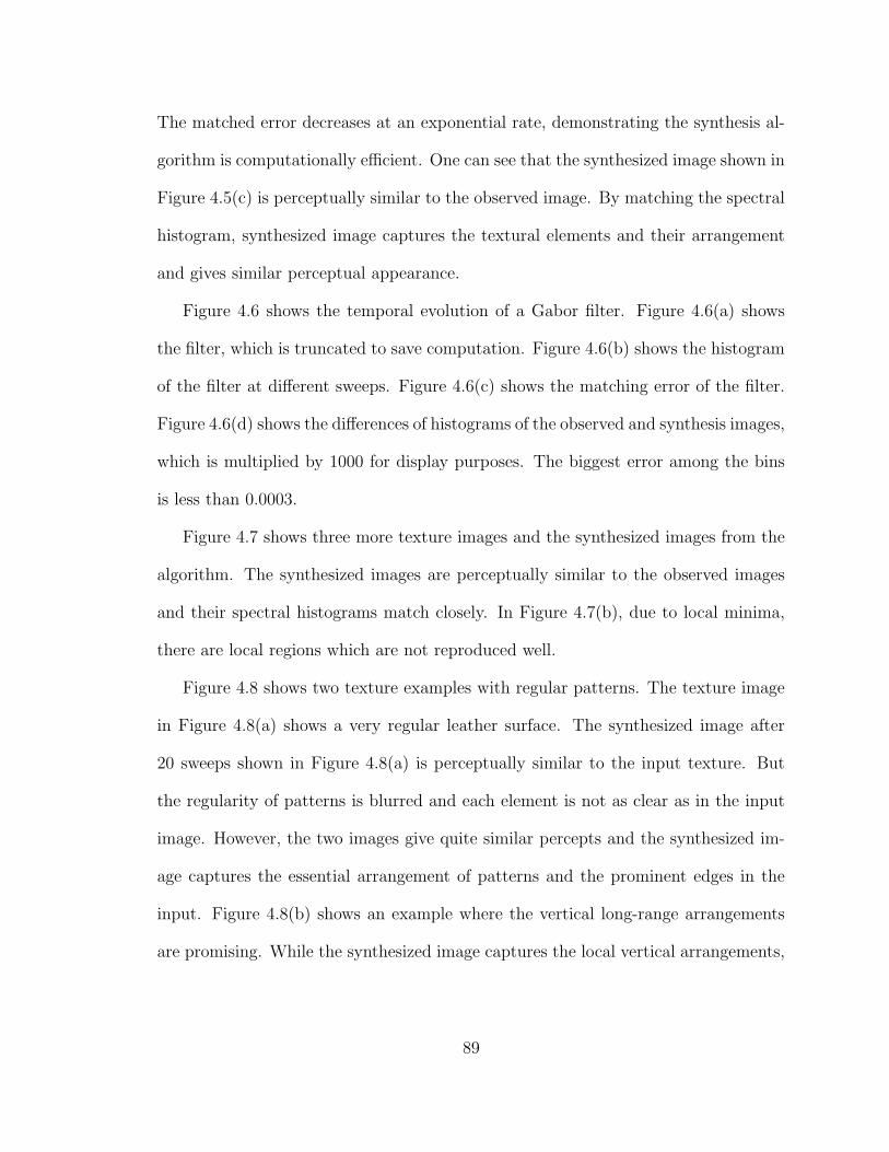
The matched error decreases at an exponential rate, demonstrating the synthesis al-
gorithm is computationally efficient. One can see that the synthesized image shown in
Figure 4.5(c) is perceptually similar to the observed image. By matching the spectral
histogram, synthesized image captures the textural elements and their arrangement
and gives similar perceptual appearance.
Figure 4.6 shows the temporal evolution of a Gabor filter. Figure 4.6(a) shows
the filter, which is truncated to save computation. Figure 4.6(b) shows the histogram
of the filter at different sweeps. Figure 4.6(c) shows the matching error of the filter.
Figure 4.6(d) shows the differences of histograms of the observed and synthesis images,
which is multiplied by 1000 for display purposes. The biggest error among the bins
is less than 0.0003.
Figure 4.7 shows three more texture images and the synthesized images from the
algorithm. The synthesized images are perceptually similar to the observed images
and their spectral histograms match closely. In Figure 4.7(b), due to local minima,
there are local regions which are not reproduced well.
Figure 4.8 shows two texture examples with regular patterns. The texture image
in Figure 4.8(a) shows a very regular leather surface. The synthesized image after
20 sweeps shown in Figure 4.8(a) is perceptually similar to the input texture. But
the regularity of patterns is blurred and each element is not as clear as in the input
image. However, the two images give quite similar percepts and the synthesized im-
age captures the essential arrangement of patterns and the prominent edges in the
input. Figure 4.8(b) shows an example where the vertical long-range arrangements
are promising. While the synthesized image captures the local vertical arrangements,
89

(a) (b)
0 2 4 6 8 10 12 140
5
10
15
20
25
(c) (d)
Figure 4.5: Texture image synthesis by matching observed statistics. (a) Observedtexture image. (b) Initial image. (c) Synthesized image after 14 sweeps. (d) Thetotal matched error with respect to sweeps.
90
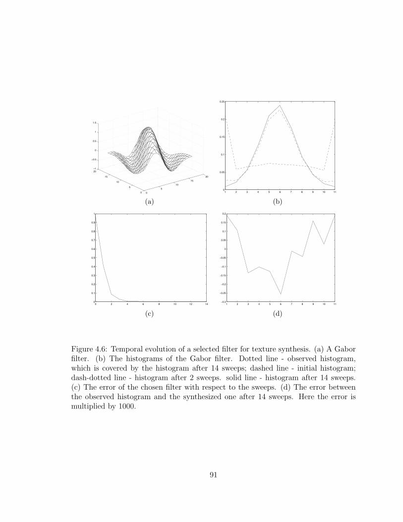
0
5
10
15
20
0
5
10
15
20−1
−0.5
0
0.5
1
1.5
1 2 3 4 5 6 7 8 9 10 110
0.05
0.1
0.15
0.2
0.25
(a) (b)
0 2 4 6 8 10 12 140
0.1
0.2
0.3
0.4
0.5
0.6
0.7
0.8
0.9
1
1 2 3 4 5 6 7 8 9 10 11−0.3
−0.25
−0.2
−0.15
−0.1
−0.05
0
0.05
0.1
0.15
0.2
(c) (d)
Figure 4.6: Temporal evolution of a selected filter for texture synthesis. (a) A Gaborfilter. (b) The histograms of the Gabor filter. Dotted line - observed histogram,which is covered by the histogram after 14 sweeps; dashed line - initial histogram;dash-dotted line - histogram after 2 sweeps. solid line - histogram after 14 sweeps.(c) The error of the chosen filter with respect to the sweeps. (d) The error betweenthe observed histogram and the synthesized one after 14 sweeps. Here the error ismultiplied by 1000.
91
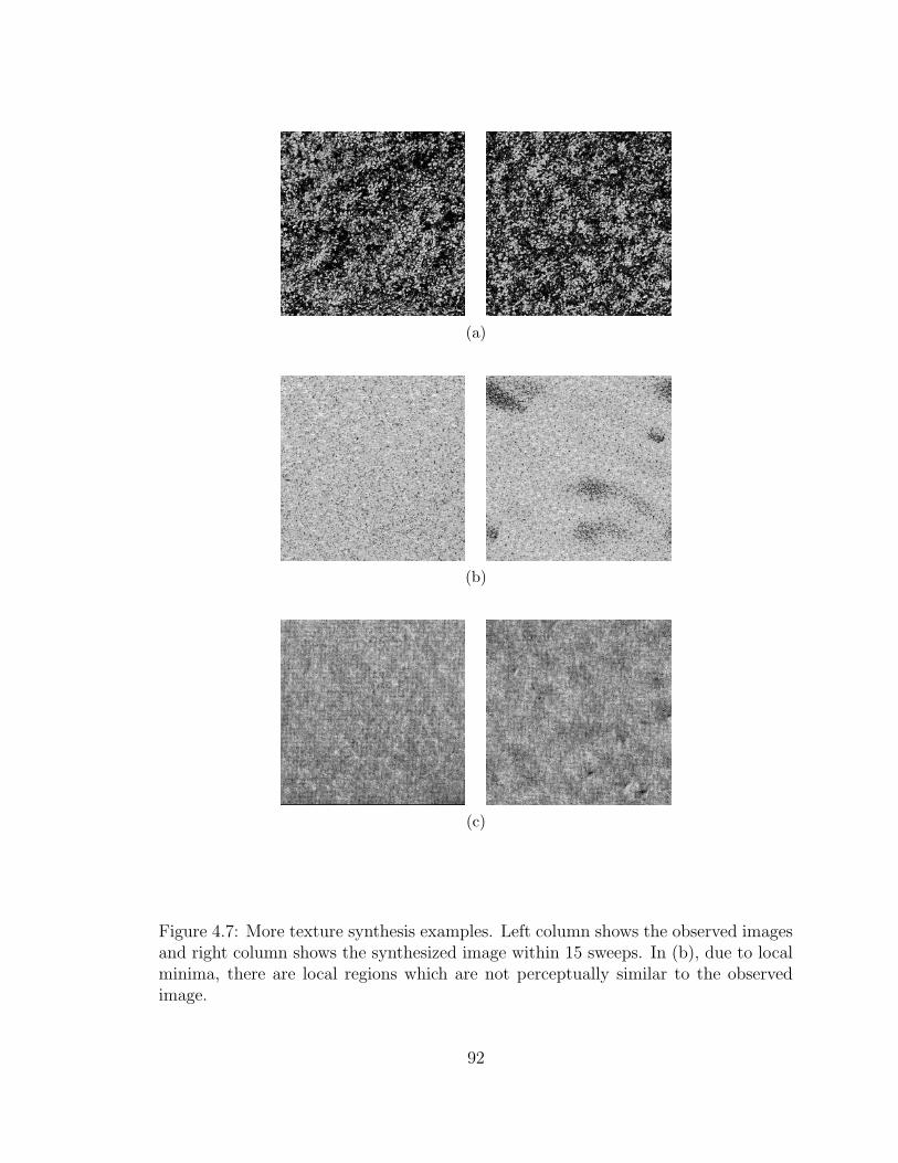
(a)
(b)
(c)
Figure 4.7: More texture synthesis examples. Left column shows the observed imagesand right column shows the synthesized image within 15 sweeps. In (b), due to localminima, there are local regions which are not perceptually similar to the observedimage.
92
it does not sufficiently capture the long-range arrangements due to that the synthe-
sized algorithm is purely local and long-range couplings are almost impossible to be
captured.
While the texture images shown above are homogeneous textures, Figure 4.9(a)
shows an intensity image consisting of several regions. Figure 4.9(c) shows the syn-
thesized image after 100 sweeps. While the spectral histogram does not capture the
spatial relationships between different regions, big regions with similar gray values
emerge along the temporal evolution. Due to the inhomogeneity, the Gibbs sam-
pler converges slower compared with homogeneous texture images as shown in Figure
4.5(d).
Figure 4.10 shows a synthesized image for a synthetic texton image. In order to
synthesize a similar texton, Zhu et al [149] [150] used a texton filter which is the
template of one texton element. Here we use the same filters as for other images. As
shown in Figure 4.10(b), the texton elements are reproduced well except in two small
regions where the MCMC is trapped into a local minimum. This example clearly
demonstrates that spectral histograms provide a generic feature for different types of
textures, eliminating the need for ad hoc features for a particular set of textures.
Figure 4.11 shows a synthetic example where there are two distinctive regions in
the original. As shown in Figure 4.11(b), the synthesized image captures the appear-
ance of both regions using the spectral histogram. Here the boundary between two
regions is not reproduced because spectral histograms do not incorporate geometric
constraints. Using some geometric constraints, the boundary may be reproduced well,
which would give a more powerful feature for images consisting of different regions.
Figure 4.12 shows an interesting result for a face image. While all the “elements” are
93
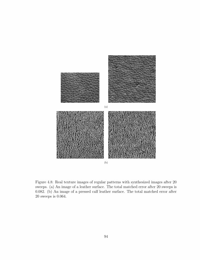
(a)
(b)
Figure 4.8: Real texture images of regular patterns with synthesized images after 20sweeps. (a) An image of a leather surface. The total matched error after 20 sweeps is0.082. (b) An image of a pressed calf leather surface. The total matched error after20 sweeps is 0.064.
94
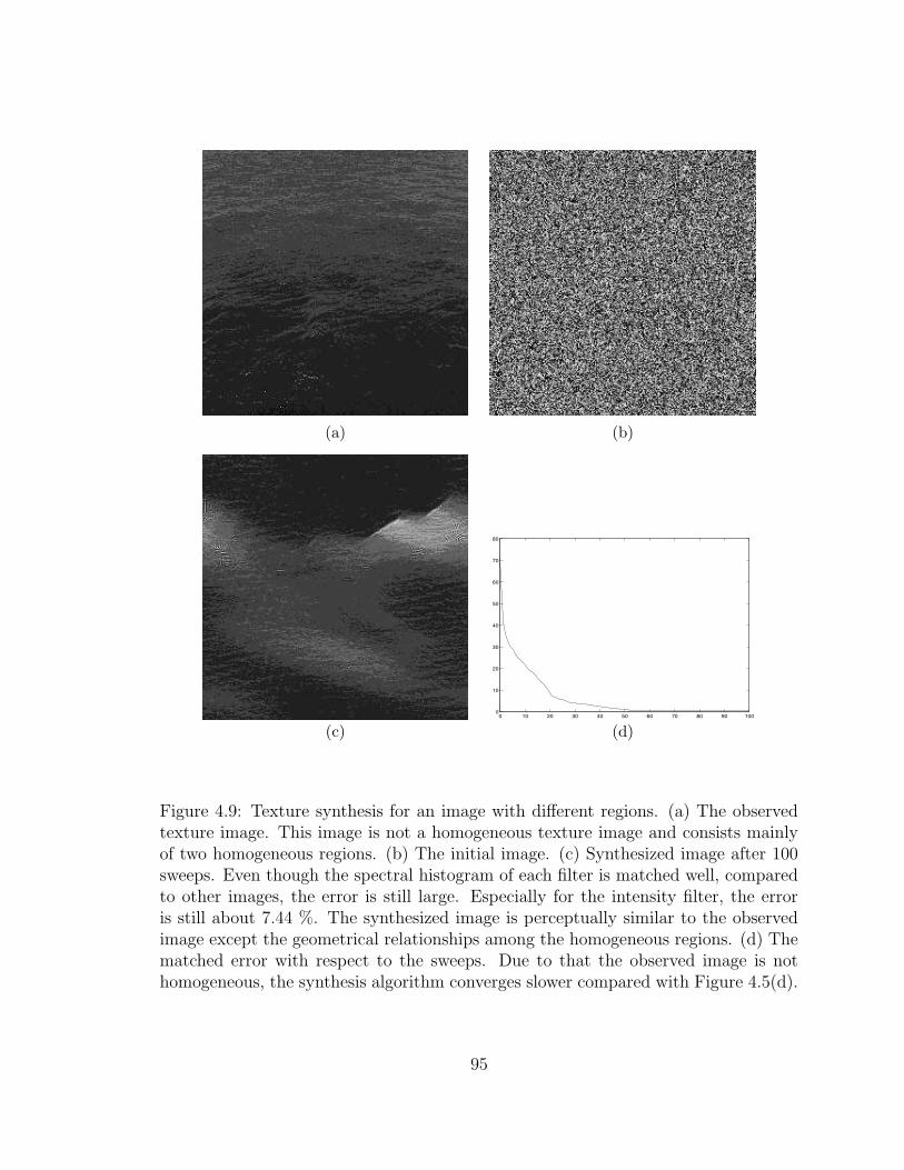
(a) (b)
0 10 20 30 40 50 60 70 80 90 1000
10
20
30
40
50
60
70
80
(c) (d)
Figure 4.9: Texture synthesis for an image with different regions. (a) The observedtexture image. This image is not a homogeneous texture image and consists mainlyof two homogeneous regions. (b) The initial image. (c) Synthesized image after 100sweeps. Even though the spectral histogram of each filter is matched well, comparedto other images, the error is still large. Especially for the intensity filter, the erroris still about 7.44 %. The synthesized image is perceptually similar to the observedimage except the geometrical relationships among the homogeneous regions. (d) Thematched error with respect to the sweeps. Due to that the observed image is nothomogeneous, the synthesis algorithm converges slower compared with Figure 4.5(d).
95
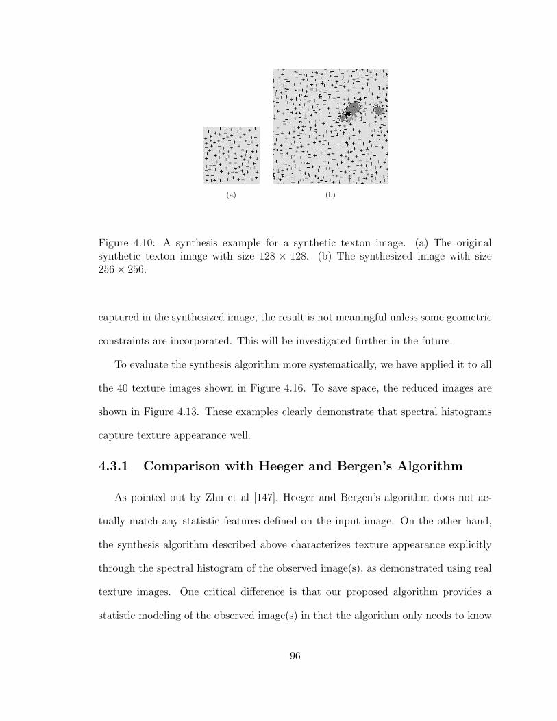
(a) (b)
Figure 4.10: A synthesis example for a synthetic texton image. (a) The originalsynthetic texton image with size 128 × 128. (b) The synthesized image with size256× 256.
captured in the synthesized image, the result is not meaningful unless some geometric
constraints are incorporated. This will be investigated further in the future.
To evaluate the synthesis algorithm more systematically, we have applied it to all
the 40 texture images shown in Figure 4.16. To save space, the reduced images are
shown in Figure 4.13. These examples clearly demonstrate that spectral histograms
capture texture appearance well.
4.3.1 Comparison with Heeger and Bergen’s Algorithm
As pointed out by Zhu et al [147], Heeger and Bergen’s algorithm does not ac-
tually match any statistic features defined on the input image. On the other hand,
the synthesis algorithm described above characterizes texture appearance explicitly
through the spectral histogram of the observed image(s), as demonstrated using real
texture images. One critical difference is that our proposed algorithm provides a
statistic modeling of the observed image(s) in that the algorithm only needs to know
96

(a) (b)
Figure 4.11: A synthesis example for an image consisting of two regions. (a) Theoriginal synthetic image with size 128 × 128, consisting of two intensity regions. (b)The synthesized image with size 256× 256.
(a) (b)
Figure 4.12: A synthesis example for a face image. (a) Lena image with size 347×334.(b) The synthesized image with size 256× 256.
97
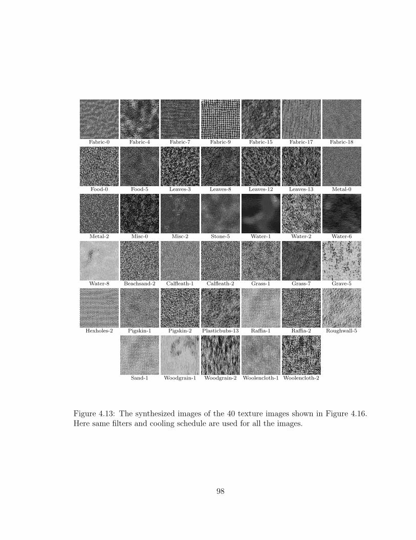
Fabric-0 Fabric-4 Fabric-7 Fabric-9 Fabric-15 Fabric-17 Fabric-18
Food-0 Food-5 Leaves-3 Leaves-8 Leaves-12 Leaves-13 Metal-0
Metal-2 Misc-0 Misc-2 Stone-5 Water-1 Water-2 Water-6
Water-8 Beachsand-2 Calfleath-1 Calfleath-2 Grass-1 Grass-7 Grave-5
Hexholes-2 Pigskin-1 Pigskin-2 Plasticbubs-13 Raffia-1 Raffia-2 Roughwall-5
Sand-1 Woodgrain-1 Woodgrain-2 Woolencloth-1 Woolencloth-2
Figure 4.13: The synthesized images of the 40 texture images shown in Figure 4.16.Here same filters and cooling schedule are used for all the images.
98
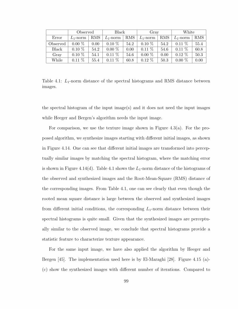
Observed Black Gray White
Error L1-norm RMS L1-norm RMS L1-norm RMS L1-norm RMS
Observed 0.00 % 0.00 0.10 % 54.2 0.10 % 54.2 0.11 % 55.4
Black 0.10 % 54.2 0.00 % 0.00 0.11 % 54.6 0.11 % 60.8
Gray 0.10 % 54.1 0.11 % 54.6 0.00 % 0.00 0.12 % 50.3
While 0.11 % 55.4 0.11 % 60.8 0.12 % 50.3 0.00 % 0.00
Table 4.1: L1-norm distance of the spectral histograms and RMS distance betweenimages.
the spectral histogram of the input image(s) and it does not need the input images
while Heeger and Bergen’s algorithm needs the input image.
For comparison, we use the texture image shown in Figure 4.3(a). For the pro-
posed algorithm, we synthesize images starting with different initial images, as shown
in Figure 4.14. One can see that different initial images are transformed into percep-
tually similar images by matching the spectral histogram, where the matching error
is shown in Figure 4.14(d). Table 4.1 shows the L1-norm distance of the histograms of
the observed and synthesized images and the Root-Mean-Square (RMS) distance of
the corresponding images. From Table 4.1, one can see clearly that even though the
rooted mean square distance is large between the observed and synthesized images
from different initial conditions, the corresponding L1-norm distance between their
spectral histograms is quite small. Given that the synthesized images are perceptu-
ally similar to the observed image, we conclude that spectral histograms provide a
statistic feature to characterize texture appearance.
For the same input image, we have also applied the algorithm by Heeger and
Bergen [45]. The implementation used here is by El-Maraghi [28]. Figure 4.15 (a)-
(c) show the synthesized images with different number of iterations. Compared to
99
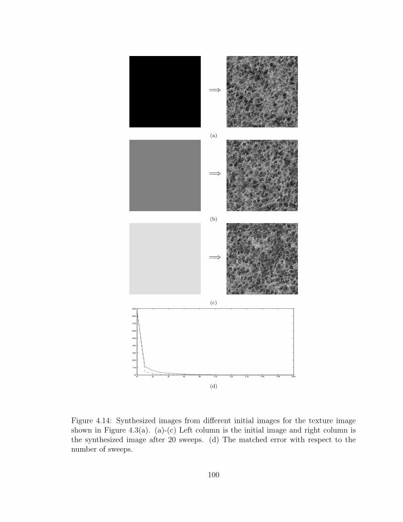
=⇒
(a)
=⇒
(b)
=⇒
(c)
0 2 4 6 8 10 12 14 16 18 200
10
20
30
40
50
60
70
80
90
(d)
Figure 4.14: Synthesized images from different initial images for the texture imageshown in Figure 4.3(a). (a)-(c) Left column is the initial image and right column isthe synthesized image after 20 sweeps. (d) The matched error with respect to thenumber of sweeps.
100
the synthesized images from our method shown in Figure 4.14(a)-(c), one can see
easily that the synthesized images in Figure 4.14(a)-(c) are perceptually similar to
the input texture image and capture texture elements and their distributions, while
the synthesized images in Figure 4.15 (a)-(c) are not percetually similar to the input
texture. As shown in Figure 4.15(d), the Heeger and Bergen’s algorithm does not
match the statistic features on which the algorithm is based and the error does not
decrease after 1 iteration. Because the Heeger and Bergen’s algorithm used Laplacian
of Gaussian paramid, we choose LoG and local filters for the spectral histogram here
for a fair comparison.
4.4 Texture Classification
Texture classification is closely related to texture segmentation and content-based
image retrieval. Here we demonstrate the discriminative power of spectral histograms.
A texture image database is given first and we extract spectral histograms for each
image in the database. The classification here is then to classify all the pixels or
selected pixels in an input image.
Given a database with M texture images, we represent each image by its average
spectral histogram Hobsm at a given integration scale. We use a minimum-distance
classifier, given by
m∗(v) = minm
D(HI(v), Hobsm). (4.11)
Here D is a similarity measure and χ2-statistic is used.
We use a texture image database available on-line at http://www-dbv.cs.uni-
bonn.de/image/texture.tar.gz. As shown in Figure 4.16, the database we use consists
of 40 texture images from Brodatz textures [10].
101
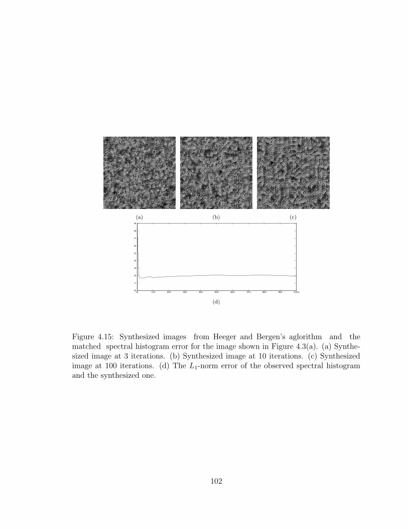
(a) (b) (c)
0 10 20 30 40 50 60 70 80 90 1000
1
2
3
4
5
6
7
8
9
(d)
Figure 4.15: Synthesized images from Heeger and Bergen’s aglorithm and thematched spectral histogram error for the image shown in Figure 4.3(a). (a) Synthe-sized image at 3 iterations. (b) Synthesized image at 10 iterations. (c) Synthesizedimage at 100 iterations. (d) The L1-norm error of the observed spectral histogramand the synthesized one.
102
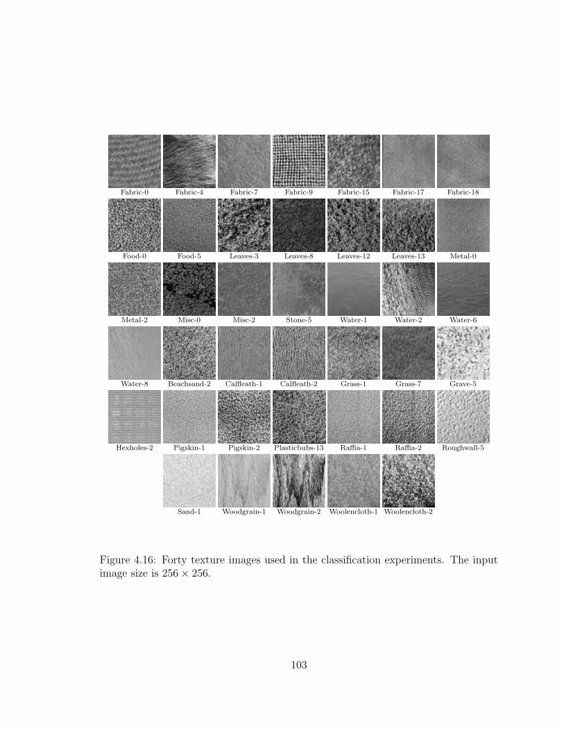
Fabric-0 Fabric-4 Fabric-7 Fabric-9 Fabric-15 Fabric-17 Fabric-18
Food-0 Food-5 Leaves-3 Leaves-8 Leaves-12 Leaves-13 Metal-0
Metal-2 Misc-0 Misc-2 Stone-5 Water-1 Water-2 Water-6
Water-8 Beachsand-2 Calfleath-1 Calfleath-2 Grass-1 Grass-7 Grave-5
Hexholes-2 Pigskin-1 Pigskin-2 Plasticbubs-13 Raffia-1 Raffia-2 Roughwall-5
Sand-1 Woodgrain-1 Woodgrain-2 Woolencloth-1 Woolencloth-2
Figure 4.16: Forty texture images used in the classification experiments. The inputimage size is 256× 256.
103

4.4.1 Classification at Fixed Scales
First we study the classification performance using the spectral histogram at a
given integration scale. As discussed above, the classification algorithm is a minimum
distance classifier and each location is classified independently from other locations.
For the database shown in Figure 4.16, we use a window of 35×35 pixels. For each
image in the database, we extract an average spectral histogram by averaging spectral
histograms extracted at a larger grid size to save computation. For classification and
content-based image retrieval, we use 8 filters to compute spectral histograms:
• The intensity filter.
• Two gradient filters Dxx and Dyy.
• Two LoG filters with T = 2 and 5.
• Three Cosine Gabor filters with T = 6 and three orientations θ = 30, 90, and
150.
Figure 4.17(a) shows the divergence between the feature vector of each image
numerically and Figure 4.17(b) shows the divergence in (a) as an image for easier
interpretation.
Each texture is divided into non-overlapping image patches with size 35 × 35.
Each image patch is classified into one of the 40 given classes using the minimum
distance classifier. Figure 4.18 shows the error rate for each image along with variance
within each image and minimum divergence of each image from the other images
in the database. The overall classification error is 4.2347%. As shown in Figure
104
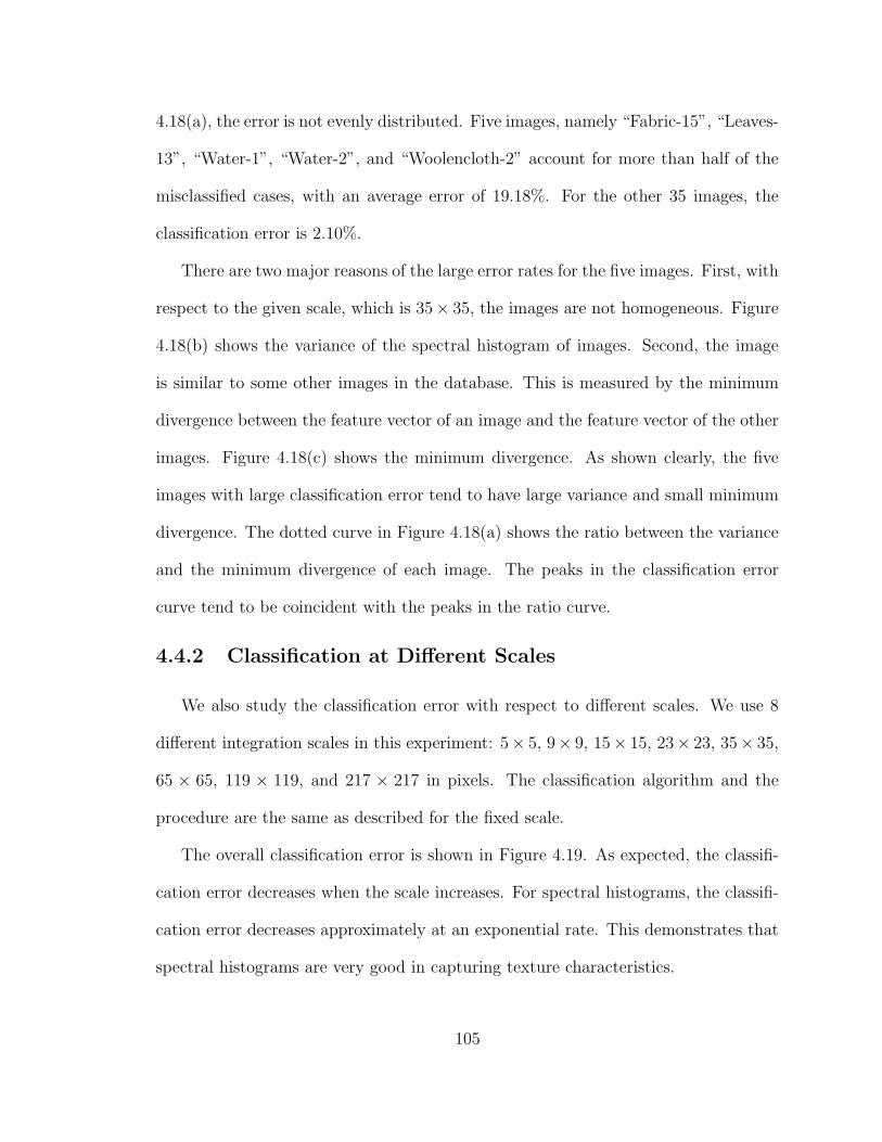
4.18(a), the error is not evenly distributed. Five images, namely “Fabric-15”, “Leaves-
13”, “Water-1”, “Water-2”, and “Woolencloth-2” account for more than half of the
misclassified cases, with an average error of 19.18%. For the other 35 images, the
classification error is 2.10%.
There are two major reasons of the large error rates for the five images. First, with
respect to the given scale, which is 35× 35, the images are not homogeneous. Figure
4.18(b) shows the variance of the spectral histogram of images. Second, the image
is similar to some other images in the database. This is measured by the minimum
divergence between the feature vector of an image and the feature vector of the other
images. Figure 4.18(c) shows the minimum divergence. As shown clearly, the five
images with large classification error tend to have large variance and small minimum
divergence. The dotted curve in Figure 4.18(a) shows the ratio between the variance
and the minimum divergence of each image. The peaks in the classification error
curve tend to be coincident with the peaks in the ratio curve.
4.4.2 Classification at Different Scales
We also study the classification error with respect to different scales. We use 8
different integration scales in this experiment: 5× 5, 9× 9, 15× 15, 23× 23, 35× 35,
65 × 65, 119 × 119, and 217 × 217 in pixels. The classification algorithm and the
procedure are the same as described for the fixed scale.
The overall classification error is shown in Figure 4.19. As expected, the classifi-
cation error decreases when the scale increases. For spectral histograms, the classifi-
cation error decreases approximately at an exponential rate. This demonstrates that
spectral histograms are very good in capturing texture characteristics.
105
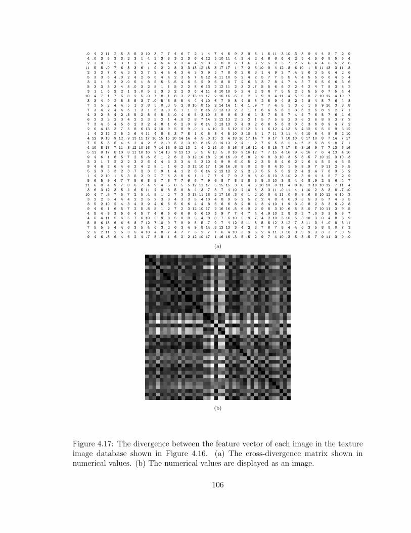
.0 4 2 11 2 5 3 5 3 10 3 7 7 4 6 7 2 1 4 7 4 5 9 3 9 5 1 5 11 3 10 3 3 9 4 4 5 7 2 9
4 .0 3 5 3 3 2 3 1 4 3 3 3 3 2 3 6 4 12 5 10 11 4 3 4 2 4 6 6 6 4 2 5 4 5 6 8 5 5 4
2 3 .0 8 2 3 1 3 1 7 4 5 4 2 3 4 4 2 9 5 8 8 6 1 6 3 2 5 8 3 7 2 2 6 4 4 6 5 2 6
11 5 8 .0 7 6 8 3 6 1 9 2 2 8 3 3 13 12 18 3 17 17 1 7 2 3 10 9 4 12 .8 6 10 1 8 11 13 3 11 .8
2 3 2 7 .0 4 3 3 2 7 2 4 4 4 3 4 3 2 9 5 7 8 6 2 6 3 1 4 9 3 7 .4 2 6 3 5 6 4 2 6
5 3 3 6 4 .0 2 4 2 6 5 4 4 2 3 5 7 5 12 4 11 10 5 2 4 2 5 7 7 5 5 4 4 5 5 6 6 4 5 4
3 2 1 8 3 2 .0 5 1 8 5 5 5 .5 4 6 5 2 9 6 8 8 7 2 6 3 3 7 8 4 7 4 3 7 6 5 6 6 3 6
5 3 3 3 3 4 5 .0 3 2 5 1 1 5 2 2 8 6 13 2 12 11 2 3 2 .7 5 5 6 6 2 2 4 2 4 7 8 3 5 2
3 1 1 6 2 2 1 3 .0 5 3 3 3 2 2 3 6 4 11 4 10 10 5 2 4 2 3 6 7 5 5 2 3 5 5 6 7 5 4 4
10 4 7 1 7 6 8 2 5 .0 7 .8 1 8 3 2 13 11 17 2 16 16 .6 6 2 3 9 8 4 11 .4 5 9 .8 7 10 12 4 10 .7
3 3 4 9 2 5 5 5 3 7 .0 5 5 5 5 4 4 4 10 6 7 9 8 4 8 5 2 5 9 4 8 2 4 8 4 5 7 6 4 8
7 3 5 2 4 4 5 1 3 .8 5 .0 .3 5 2 .8 10 8 15 2 14 14 1 4 1 .9 7 7 4 8 1 3 6 1 6 9 10 3 8 .8
7 3 4 2 4 4 5 1 3 1 5 .3 .0 5 1 1 9 8 15 .9 13 13 2 3 1 1 6 6 5 8 2 3 6 2 5 8 9 2 7 1
4 3 2 8 4 2 .5 5 2 8 5 5 5 .0 4 6 5 3 10 5 9 9 6 3 6 4 3 7 8 5 7 4 5 7 6 5 7 6 4 6
6 2 3 3 3 3 4 2 2 3 5 2 1 4 .0 2 8 7 14 2 12 13 2 3 2 1 5 7 5 8 3 3 6 2 6 8 9 3 7 2
7 3 4 3 4 5 6 2 3 2 4 .8 1 6 2 .0 9 8 14 3 13 13 3 4 3 2 6 6 5 8 3 3 6 3 6 8 9 4 7 2
2 6 4 13 3 7 5 8 6 13 4 10 9 5 8 9 .0 1 4 10 2 5 12 5 12 8 1 6 12 4 13 5 4 12 6 5 5 9 3 12
1 4 2 12 2 5 2 6 4 11 4 8 8 3 7 8 1 .0 5 8 4 5 10 3 10 6 1 7 11 3 11 4 4 10 6 4 5 8 2 10
4 12 9 18 9 12 9 13 11 17 10 15 15 10 14 14 4 5 .0 15 2 4 18 10 17 14 7 9 17 7 18 10 8 17 10 8 7 14 7 17
7 5 5 3 5 4 6 2 4 2 6 2 .9 5 2 3 10 8 15 .0 14 13 2 4 1 2 7 6 5 8 2 4 6 2 5 8 9 .8 7 1
4 10 8 17 7 11 8 12 10 16 7 14 13 9 12 13 2 4 2 14 .0 5 16 9 16 12 4 8 15 7 17 8 8 16 9 7 7 13 6 16
5 11 8 17 8 10 8 11 10 16 9 14 13 9 13 13 5 5 4 13 5 .0 16 9 16 12 7 7 15 4 16 9 6 16 7 6 4 13 4 16
9 4 6 1 6 5 7 2 5 .6 8 1 2 6 2 3 12 10 18 2 16 16 .0 6 .8 2 9 8 3 10 .3 5 8 .5 7 10 12 3 10 .3
3 3 1 7 2 2 2 3 2 6 4 4 3 3 3 4 5 3 10 4 9 9 6 .0 5 2 3 5 8 4 6 2 2 6 4 5 5 4 3 5
9 4 6 2 6 4 6 2 4 2 8 1 1 6 2 3 12 10 17 1 16 16 .8 5 .0 2 9 8 4 10 1 5 8 .9 7 9 11 2 9 .5
5 2 3 3 3 2 3 .7 2 3 5 .9 1 4 1 2 8 6 14 2 12 12 2 2 2 .0 5 5 5 6 2 2 4 2 4 7 8 3 5 2
1 4 2 10 1 5 3 5 3 9 2 7 6 3 5 6 1 1 7 7 4 7 9 3 9 5 .0 5 10 3 10 2 3 9 4 4 5 7 2 9
5 6 5 9 4 7 7 5 6 8 5 7 6 7 7 6 6 7 9 6 8 7 8 5 8 5 5 .0 10 3 8 4 4 8 .9 2 5 6 4 7
11 6 8 4 9 7 8 6 7 4 9 4 5 8 5 5 12 11 17 5 15 15 3 8 4 5 10 10 .0 11 4 8 10 3 10 10 12 7 11 4
3 6 3 12 3 5 4 6 5 11 4 8 8 5 8 8 4 3 7 8 7 4 10 4 10 6 3 3 11 .0 11 4 1 10 2 3 3 8 .7 10
10 4 7 .8 7 5 7 2 5 .4 8 1 2 7 3 3 13 11 18 2 17 16 .3 6 1 2 10 8 4 11 .0 6 9 .6 8 10 12 4 10 .3
3 2 2 6 .4 4 4 2 2 5 2 3 3 4 3 3 5 4 10 4 8 9 5 2 5 2 2 4 8 4 6 .0 3 5 3 5 7 4 3 5
3 5 2 10 2 4 3 4 3 9 4 6 6 5 6 6 4 4 8 6 8 6 8 2 8 4 3 4 10 1 9 3 .0 8 2 3 3 6 .9 8
9 4 6 1 6 5 7 2 5 .8 8 1 2 7 2 3 12 10 17 2 16 16 .5 6 .9 2 9 8 3 10 .6 5 8 .0 7 10 11 3 9 .5
4 5 4 8 3 5 6 4 5 7 4 6 5 6 6 6 6 6 10 5 9 7 7 4 7 4 4 .9 10 2 8 3 2 7 .0 3 3 5 3 7
4 6 4 11 5 6 5 7 6 10 5 9 8 5 8 8 5 4 8 8 7 6 10 5 9 7 4 2 10 3 10 5 3 10 3 .0 4 8 3 9
5 8 6 13 6 6 6 8 7 12 7 10 9 7 9 9 5 5 7 9 7 4 12 5 11 8 5 5 12 3 12 7 3 11 3 4 .0 8 3 11
7 5 5 3 4 4 6 3 5 4 6 3 2 6 3 4 9 8 14 .8 13 13 3 4 2 3 7 6 7 8 4 4 6 3 5 8 8 .0 7 3
2 5 2 11 2 5 3 5 4 10 4 8 7 4 7 7 3 2 7 7 6 4 10 3 9 5 2 4 11 .7 10 3 .9 9 3 3 3 7 .0 9
9 4 6 .8 6 4 6 2 4 .7 8 .8 1 6 2 2 12 10 17 1 16 16 .3 5 .5 2 9 7 4 10 .3 5 8 .5 7 9 11 3 9 .0
(a)
(b)
Figure 4.17: The divergence between the feature vector of each image in the textureimage database shown in Figure 4.16. (a) The cross-divergence matrix shown innumerical values. (b) The numerical values are displayed as an image.
106
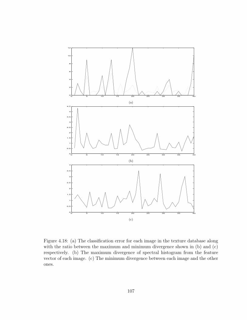
0 5 10 15 20 25 30 35 400
2
4
6
8
10
12
(a)
0 5 10 15 20 25 30 35 400
0.5
1
1.5
2
2.5
3
3.5
4
4.5
(b)
0 5 10 15 20 25 30 35 400
0.5
1
1.5
2
2.5
3
3.5
4
(c)
Figure 4.18: (a) The classification error for each image in the texture database alongwith the ratio between the maximum and minimum divergence shown in (b) and (c)respectively. (b) The maximum divergence of spectral histogram from the featurevector of each image. (c) The minimum divergence between each image and the otherones.
107
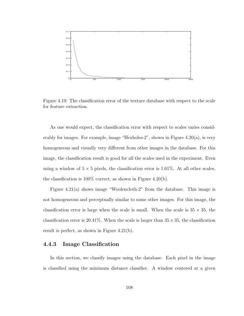
0 50 100 150 200 2500
0.1
0.2
0.3
0.4
0.5
0.6
0.7
Figure 4.19: The classification error of the texture database with respect to the scalefor feature extraction.
As one would expect, the classification error with respect to scales varies consid-
erably for images. For example, image “Hexholes-2”, shown in Figure 4.20(a), is very
homogeneous and visually very different from other images in the database. For this
image, the classification result is good for all the scales used in the experiment. Even
using a window of 5 × 5 pixels, the classification error is 1.61%. At all other scales,
the classification is 100% correct, as shown in Figure 4.20(b).
Figure 4.21(a) shows image “Woolencloth-2” from the database. This image is
not homogeneous and perceptually similar to some other images. For this image, the
classification error is large when the scale is small. When the scale is 35 × 35, the
classification error is 20.41%. When the scale is larger than 35× 35, the classification
result is perfect, as shown in Figure 4.21(b).
4.4.3 Image Classification
In this section, we classify images using the database. Each pixel in the image
is classified using the minimum distance classifier. A window centered at a given
108
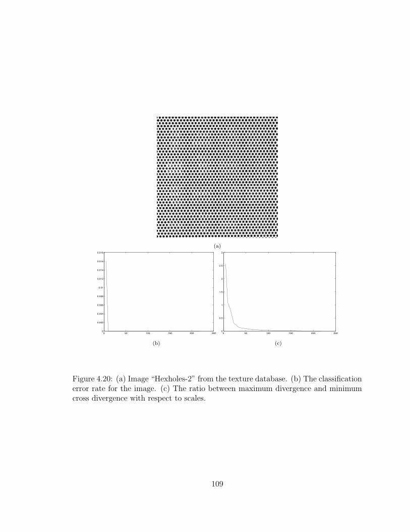
(a)
0 50 100 150 200 2500
0.002
0.004
0.006
0.008
0.01
0.012
0.014
0.016
0.018
0 50 100 150 200 2500
0.5
1
1.5
2
2.5
3
(b) (c)
Figure 4.20: (a) Image “Hexholes-2” from the texture database. (b) The classificationerror rate for the image. (c) The ratio between maximum divergence and minimumcross divergence with respect to scales.
109

(a)
0 50 100 150 200 2500
0.1
0.2
0.3
0.4
0.5
0.6
0.7
0.8
0.9
1
0 50 100 150 200 2500
20
40
60
80
100
120
140
160
180
(b) (c)
Figure 4.21: (a) Image “Woolencloth-2” from the texture database. (b) The clas-sification error rate for the image. (c) The ratio between maximum divergence andminimum cross divergence with respect to scales.
110
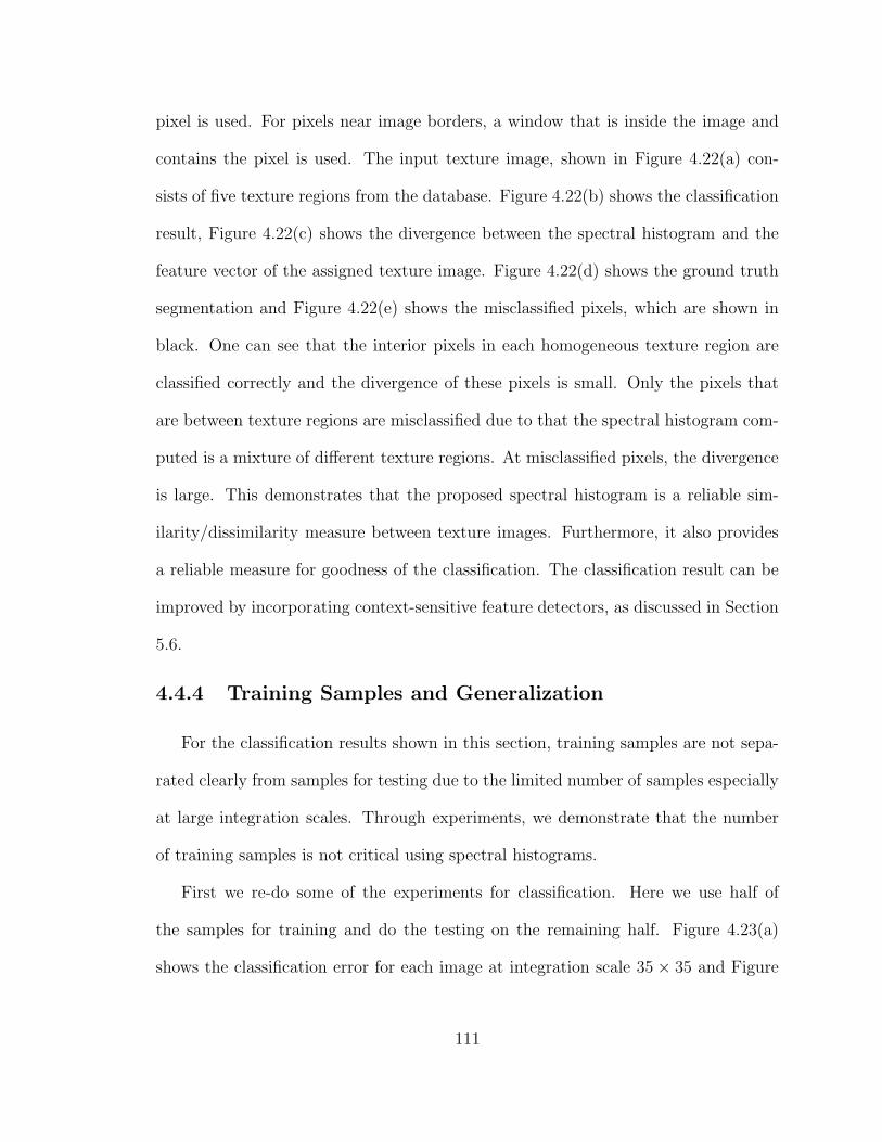
pixel is used. For pixels near image borders, a window that is inside the image and
contains the pixel is used. The input texture image, shown in Figure 4.22(a) con-
sists of five texture regions from the database. Figure 4.22(b) shows the classification
result, Figure 4.22(c) shows the divergence between the spectral histogram and the
feature vector of the assigned texture image. Figure 4.22(d) shows the ground truth
segmentation and Figure 4.22(e) shows the misclassified pixels, which are shown in
black. One can see that the interior pixels in each homogeneous texture region are
classified correctly and the divergence of these pixels is small. Only the pixels that
are between texture regions are misclassified due to that the spectral histogram com-
puted is a mixture of different texture regions. At misclassified pixels, the divergence
is large. This demonstrates that the proposed spectral histogram is a reliable sim-
ilarity/dissimilarity measure between texture images. Furthermore, it also provides
a reliable measure for goodness of the classification. The classification result can be
improved by incorporating context-sensitive feature detectors, as discussed in Section
5.6.
4.4.4 Training Samples and Generalization
For the classification results shown in this section, training samples are not sepa-
rated clearly from samples for testing due to the limited number of samples especially
at large integration scales. Through experiments, we demonstrate that the number
of training samples is not critical using spectral histograms.
First we re-do some of the experiments for classification. Here we use half of
the samples for training and do the testing on the remaining half. Figure 4.23(a)
shows the classification error for each image at integration scale 35 × 35 and Figure
111
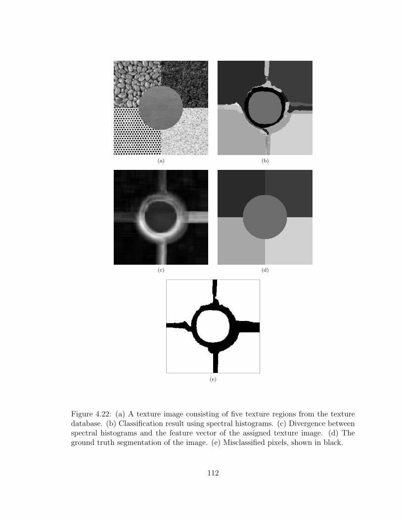
(a) (b)
(c) (d)
(e)
Figure 4.22: (a) A texture image consisting of five texture regions from the texturedatabase. (b) Classification result using spectral histograms. (c) Divergence betweenspectral histograms and the feature vector of the assigned texture image. (d) Theground truth segmentation of the image. (e) Misclassified pixels, shown in black.
112

0 5 10 15 20 25 30 35 400
0.05
0.1
0.15
0.2
0.25
0 10 20 30 40 50 60 700
0.1
0.2
0.3
0.4
0.5
0.6
0.7
(a) (b)
Figure 4.23: (a) The classification error for each image in the database at integrationscale 35×35. (b) The classification error at different integration scales. In both cases,solid line – training is done using half of the samples; dashed line – training is doneusing all the samples.
4.23(b) shows the overall error at different integration scales along with the results
shown before. While the classification error varies from image to image using different
training samples, the overall classification error does not change much.
We also examine the influence of the ratio of testing samples to training samples.
Figure 4.24 shows the classification error with respect to the ratio of testing samples
to training samples at integration scales 23 × 23 and 35 × 35. It demonstrates that
the spectral histogram captures texture characteristics well from a small number of
training samples.
4.4.5 Comparison with Existing Approaches
Recently, Randen and Husoy did an extensive comparative study for texture clas-
sification using different filtering-based methods [108]. We have applied our method
113
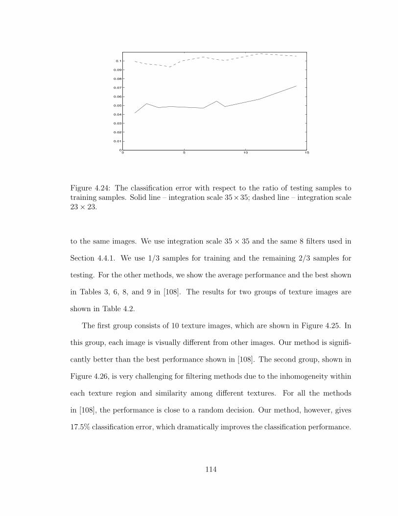
0 5 10 150
0.01
0.02
0.03
0.04
0.05
0.06
0.07
0.08
0.09
0.1
Figure 4.24: The classification error with respect to the ratio of testing samples totraining samples. Solid line – integration scale 35×35; dashed line – integration scale23× 23.
to the same images. We use integration scale 35 × 35 and the same 8 filters used in
Section 4.4.1. We use 1/3 samples for training and the remaining 2/3 samples for
testing. For the other methods, we show the average performance and the best shown
in Tables 3, 6, 8, and 9 in [108]. The results for two groups of texture images are
shown in Table 4.2.
The first group consists of 10 texture images, which are shown in Figure 4.25. In
this group, each image is visually different from other images. Our method is signifi-
cantly better than the best performance shown in [108]. The second group, shown in
Figure 4.26, is very challenging for filtering methods due to the inhomogeneity within
each texture region and similarity among different textures. For all the methods
in [108], the performance is close to a random decision. Our method, however, gives
17.5% classification error, which dramatically improves the classification performance.
114

Texture Existing methods in [108] Proposedgroup Average Best method
Figure 4.25 47.9 % 32.3 % 9.7 %Figure 4.26 89.0 % 84.9 % 17.5 %
Table 4.2: Classification errors of methods shown in [108] and our method
This comparison clearly suggests that classification based on filtering output is
not sufficient in characterizing texture appearance and an integration after filtering
must be done as Malik and Perona pointed out that a nonlinearity after filtering is
necessary for texture discrimination [87].
This comparison along with the results on texture synthesis strongly indicates
that spectral histogram is necessary in order to capture texture appearance.
4.5 Content-based Image Retrieval
Content-based image retrieval is closely related to image classification and segmen-
tation. Given some desired feature statistics, one would like to find all the images in a
given database that is similar to the given feature statistics. For example, one can use
intensity histogram and other statistics that are easy to compute to efficiently find
images. Because those heuristic-based features do not provide sufficient modeling for
images, it is not possible to provide any theoretical justification about the result. As
shown in previous sections on texture image synthesis and classification, spectral his-
tograms provide a statistically sufficient model for natural homogeneous textures. In
this section, we demonstrate how the spectral histogram and the associated similarity
measure can be used to retrieve images that contain perceptually similar region.
115
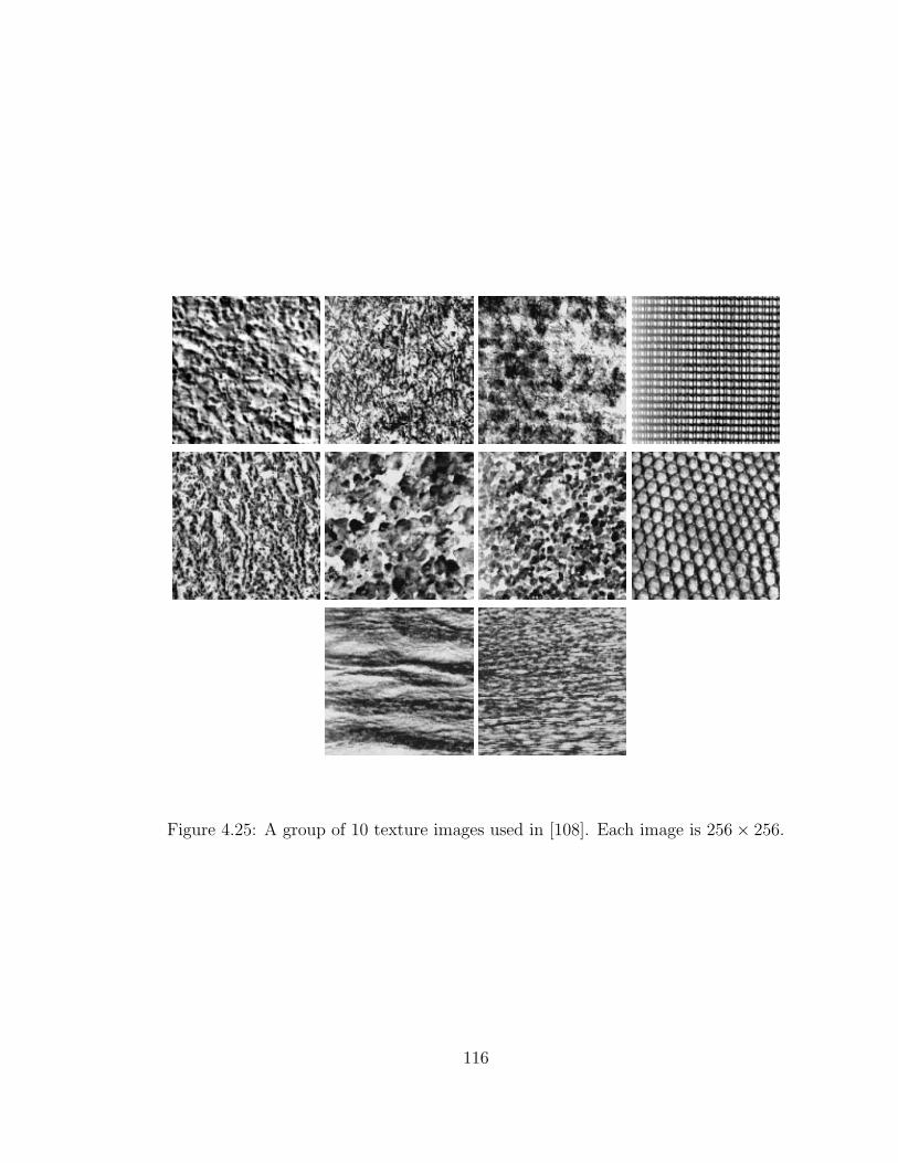
Figure 4.25: A group of 10 texture images used in [108]. Each image is 256× 256.
116
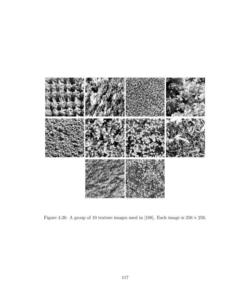
Figure 4.26: A group of 10 texture images used in [108]. Each image is 256× 256.
117

For content-based image retrieval, we use a database consisting of 100 texture
images each of which is composed of five texture regions from the texture image
database used in the classification example. For a given image patch, we extract
its spectral histogram as its footprint. As mentioned before, the same filters for
classification are used. Then we try to identify the best match in a texture image in
the database. To save some computation, we only compute spectral histogram on a
coarsely sampled grid.
Figure 4.27 shows an example. Figure 4.27(a) shows an input image patch with
size of 35× 35 in pixels. Figure 4.27(b) shows the minimum divergence between the
given patch and the images in the database. It shows clearly that there is a step edge.
The images that have a smaller matched error than the threshold given by the step
edge all actually contain the input match. Figure 4.27(c) shows the first nine image
with the matched error. The matched errors of the first eight images are much smaller
than the ninth image. This demonstrates that the spectral histogram characterizes
texture appearance very well for homogeneous textures.
Figure 4.28 shows another example. Here the texture is not very homogeneous
and consists of regular texture patterns. Figure 4.28(a) shows the input image patch
with size of 53 × 53 in pixels. Figure 4.28(b) shows the matched error of the 100
images in the database. While the edge is not a step edge, a ramp edge can be seen
clearly. As in Figure 4.27, this ramp edge defines a threshold for image that actually
contain patches that are perceptually similar to the given patch. Figure 4.28(c) shows
the first 12 images with the smallest match errors. All of them are correctly retrieved.
From these two examples, we can see a fixed threshold might be chosen. In both
cases, the threshold is around 0.25. Because χ2-statistic obeys a χ2 distribution, a
118

0
10
20
30
40
50
60
70
80
90
10
00 1 2 3 4 5 6 7
(a)
(b)
0.0
73306
0.0
88377
0.0
91331
0.0
92707
0.0
92707
0.1
16957
0.2
53079
0.2
57533
2.4
76219
Figu
re4.27:
Image
retrievalresu
ltfrom
a100-im
agedatab
aseusin
ga
givenim
agepatch
based
onsp
ectralhistogram
s.(a)
Input
image
patch
with
size35×
35.(b
)T
he
sortedm
atched
errorfor
the
100im
agesin
the
datab
ase.(c)
The
first
nin
eim
agew
ithsm
allesterrors.
119
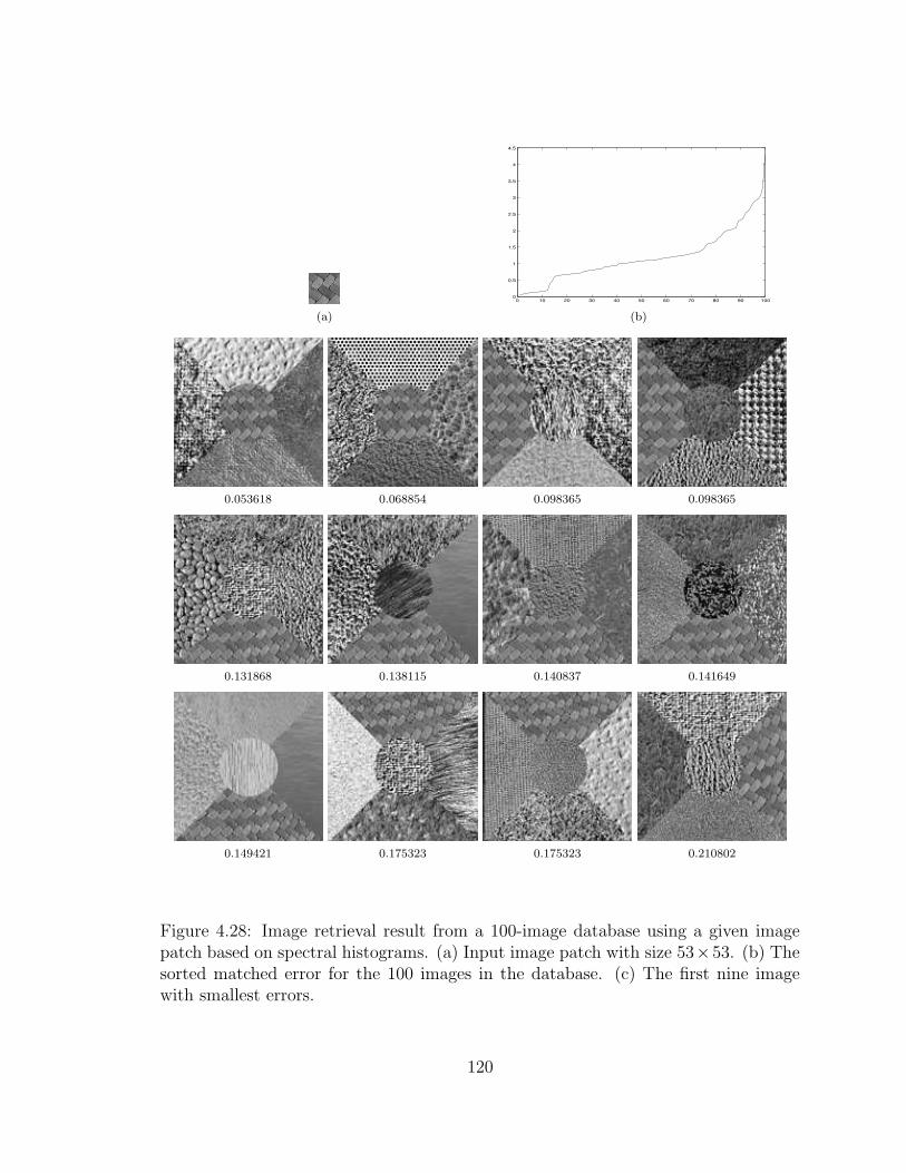
0 10 20 30 40 50 60 70 80 90 1000
0.5
1
1.5
2
2.5
3
3.5
4
4.5
(a) (b)
0.053618 0.068854 0.098365 0.098365
0.131868 0.138115 0.140837 0.141649
0.149421 0.175323 0.175323 0.210802
Figure 4.28: Image retrieval result from a 100-image database using a given imagepatch based on spectral histograms. (a) Input image patch with size 53×53. (b) Thesorted matched error for the 100 images in the database. (c) The first nine imagewith smallest errors.
120
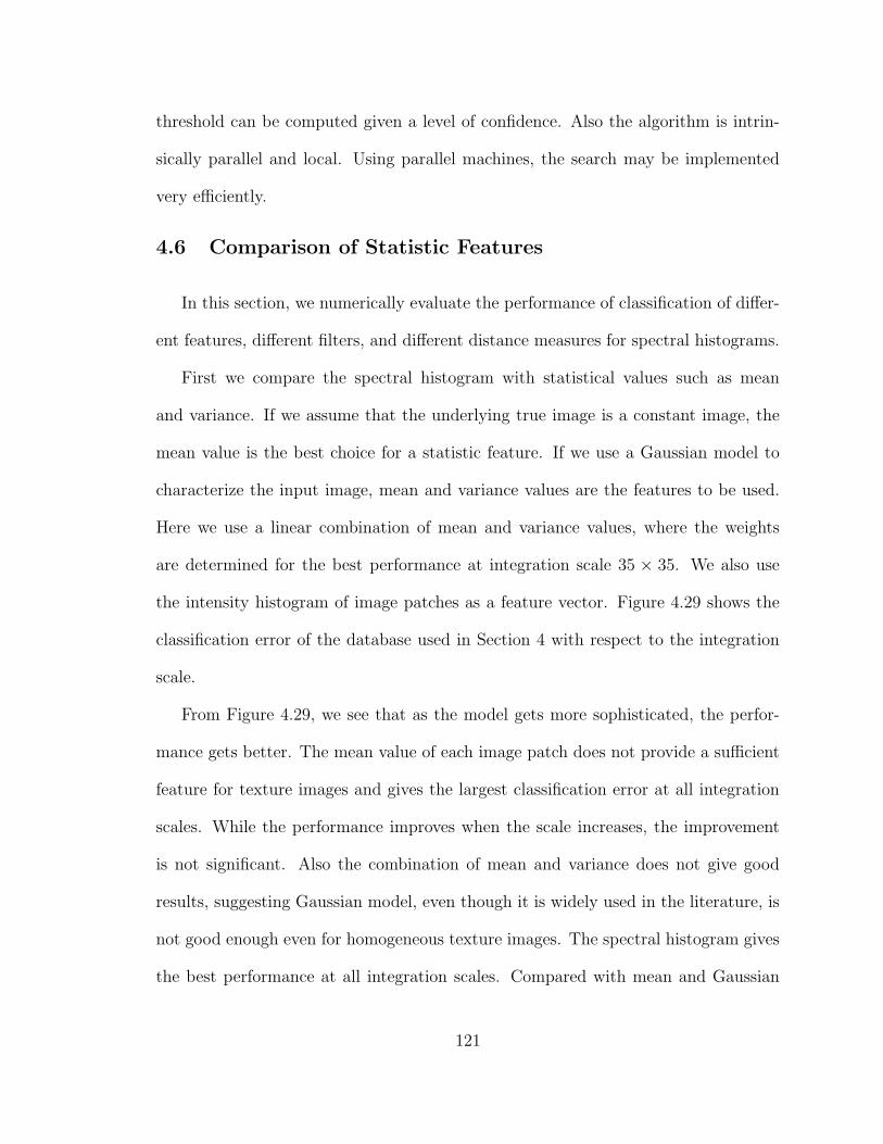
threshold can be computed given a level of confidence. Also the algorithm is intrin-
sically parallel and local. Using parallel machines, the search may be implemented
very efficiently.
4.6 Comparison of Statistic Features
In this section, we numerically evaluate the performance of classification of differ-
ent features, different filters, and different distance measures for spectral histograms.
First we compare the spectral histogram with statistical values such as mean
and variance. If we assume that the underlying true image is a constant image, the
mean value is the best choice for a statistic feature. If we use a Gaussian model to
characterize the input image, mean and variance values are the features to be used.
Here we use a linear combination of mean and variance values, where the weights
are determined for the best performance at integration scale 35 × 35. We also use
the intensity histogram of image patches as a feature vector. Figure 4.29 shows the
classification error of the database used in Section 4 with respect to the integration
scale.
From Figure 4.29, we see that as the model gets more sophisticated, the perfor-
mance gets better. The mean value of each image patch does not provide a sufficient
feature for texture images and gives the largest classification error at all integration
scales. While the performance improves when the scale increases, the improvement
is not significant. Also the combination of mean and variance does not give good
results, suggesting Gaussian model, even though it is widely used in the literature, is
not good enough even for homogeneous texture images. The spectral histogram gives
the best performance at all integration scales. Compared with mean and Gaussian
121
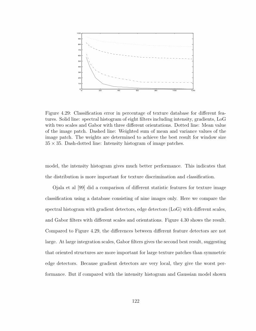
0 20 40 60 80 100 1200
10
20
30
40
50
60
70
80
90
100
Figure 4.29: Classification error in percentage of texture database for different fea-tures. Solid line: spectral histogram of eight filters including intensity, gradients, LoGwith two scales and Gabor with three different orientations. Dotted line: Mean valueof the image patch. Dashed line: Weighted sum of mean and variance values of theimage patch. The weights are determined to achieve the best result for window size35× 35. Dash-dotted line: Intensity histogram of image patches.
model, the intensity histogram gives much better performance. This indicates that
the distribution is more important for texture discrimination and classification.
Ojala et al [99] did a comparison of different statistic features for texture image
classification using a database consisting of nine images only. Here we compare the
spectral histogram with gradient detectors, edge detectors (LoG) with different scales,
and Gabor filters with different scales and orientations. Figure 4.30 shows the result.
Compared to Figure 4.29, the differences between different feature detectors are not
large. At large integration scales, Gabor filters gives the second best result, suggesting
that oriented structures are more important for large texture patches than symmetric
edge detectors. Because gradient detectors are very local, they give the worst per-
formance. But if compared with the intensity histogram and Gaussian model shown
122

0 20 40 60 80 100 1200
10
20
30
40
50
60
70
80
Figure 4.30: Classification error in percentage of the texture database for differentfilters. Solid line: spectral histogram of eight filters including intensity, gradients,LoG with two scales and Gabor with three different orientations. Dotted line: Gra-dient filters Dxx and Dyy; Dashed line: Laplacian of Gaussian filters LoG(
√2/2),
LoG(1), and LoG(2). Dash-dotted line: Six Cosine Gabor filters with T = 4 and sixorientations θ = 0, 30, 60, 90, 120, and 150.
in Figure 4.29, it still gives a very good performance. This again confirms that the
distribution of local features is important for texture classification and segmentation.
Finally, for spectral histograms, we compare different distance measures. As given
in equations (4.4) (4.5), and (4.6), here we use L1-norm, L2-norm, Kullback-Leibler
divergence, and χ2-statistic. As shown in Figure 4.31, the differences between different
distance measures are very small, suggesting that spectral histograms do not depend
on the particular form of distance measure. This observation is different from the
conclusion in [107], where the authors claim χ2-statistic consistently gives the best
performance. The reason for the differences is that spectral histograms in our case are
derived by integrating information from the same window at different scales, while
different windows are used in [107] at different scales.
123
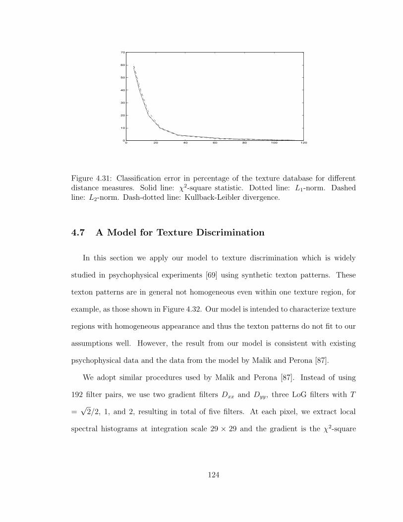
0 20 40 60 80 100 1200
10
20
30
40
50
60
70
Figure 4.31: Classification error in percentage of the texture database for differentdistance measures. Solid line: χ2-square statistic. Dotted line: L1-norm. Dashedline: L2-norm. Dash-dotted line: Kullback-Leibler divergence.
4.7 A Model for Texture Discrimination
In this section we apply our model to texture discrimination which is widely
studied in psychophysical experiments [69] using synthetic texton patterns. These
texton patterns are in general not homogeneous even within one texture region, for
example, as those shown in Figure 4.32. Our model is intended to characterize texture
regions with homogeneous appearance and thus the texton patterns do not fit to our
assumptions well. However, the result from our model is consistent with existing
psychophysical data and the data from the model by Malik and Perona [87].
We adopt similar procedures used by Malik and Perona [87]. Instead of using
192 filter pairs, we use two gradient filters Dxx and Dyy, three LoG filters with T
=√
2/2, 1, and 2, resulting in total of five filters. At each pixel, we extract local
spectral histograms at integration scale 29 × 29 and the gradient is the χ2-square
124
(+ O) (+ []) (L +) (L M)
(∆ →) (+ T) (+ X) (T L)
(LL ML) (R-mirror-R)
Figure 4.32: Ten synthetic texture pairs scanned from Malik and Perona [87]. Thesize is 136× 136.
distance between the spectral histograms of the two adjacent windows. Then the
gradient is averaged along each column.
The images used in our experiment are shown in Figure 4.32, which were scanned
from Malik and Perona [87]. The texture gradients for selected texture pairs (+ O)
and (R-mirror-R) from our method are shown in Figure 4.33 (b) and (d).
There are several observations that can be made from the gradient results shown
in Figure 4.33. First, the texture pattern does not give rise to a homogeneous texture
125

20 30 40 50 60 70 80 90 100 1100
20
40
60
80
100
120
(a) (b)
20 30 40 50 60 70 80 90 100 1100
5
10
15
(c) (d)
Figure 4.33: The averaged texture gradient for selected texture pairs. (a) The texturepair (+ O) as shown in Figure 4.32. (b) The texture gradient averaged along eachcolumn for (a). The horizontal axis is the column number and the vertical axis is thegradient. (c) The texture pair (R-mirror-R). (d) The averaged texture gradient for(c).
126

region, and variations within each texture region are clearly perceivable. For example,
in the texture pair (+ O), we do perceive columnar structures besides the major
texture boundary. Second, because of the inhomogeneity, the absolute value of texture
gradient should not be used directly as a measure for texture discrimination, which
was actually used by Malik and Perona [87]. As shown in Figure 4.33 (d), even though
the gradient is much weaker compared to Figure 4.33 (b), the filters still respond to
the texture variations, which is evident in Malik and Perona [87] also. However, the
texture boundary is not perceived.
Based on the above observations, we propose a texture discrimination measure as
the difference between the central peak and the maximum of adjacent side peaks. In
the (+ o) case, the central peak is 104.2320, and the left and right side peaks are
45.4100 and 34.6510 respectively, thus the discrimination measure is 58.8220. For the
(R-mirror-R) case, the central peak is 7.2310 and the left and right side peaks are
5.3580 and 11.4680 respectively, thus the measure is -4.2370, which indicates that the
two texture regions are not discriminable at all.
We calculate the proposed discrimination measure for the ten texture pairs. Table
4.3 shows the psychophysical data from [69], the data from Malik and Perona’s model
[87], and the proposed measure. Here the data from [69] was actually based on the
converted data shown in [87]. Figure 4.34 shows the data which are linearly scaled
so that the measures for (+ []) match. It is clear that our measure is consistent
with the other two except for the texture pair (L +). Our measure indicates that
that (+ O) is much easier to discriminate than the other pairs, the pair (LL, ML)
is barely discriminable with a measure of 0.2080, and the pair (R-mirror-R) is not
discriminable with a measure of -4.2370.
127
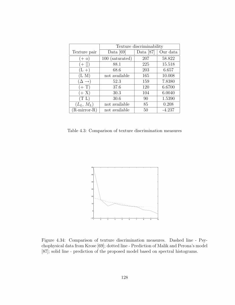
Texture discriminabilityTexture pair Data [69] Data [87] Our data
(+ o) 100 (saturated) 207 58.822(+ []) 88.1 225 15.518(L +) 68.6 203 6.657(L M) not available 165 10.008(∆ →) 52.3 159 7.8380(+ T) 37.6 120 6.6700(+ X) 30.3 104 6.0040(T L) 30.6 90 1.5390
(LL, ML) not available 85 0.208(R-mirror-R) not available 50 -4.237
Table 4.3: Comparison of texture discrimination measures
1 2 3 4 5 6 7 8 9 10−10
0
10
20
30
40
50
60
Figure 4.34: Comparison of texture discrimination measures. Dashed line - Psy-chophysical data from Krose [69]; dotted line - Prediction of Malik and Perona’s model[87]; solid line - prediction of the proposed model based on spectral histograms.
128
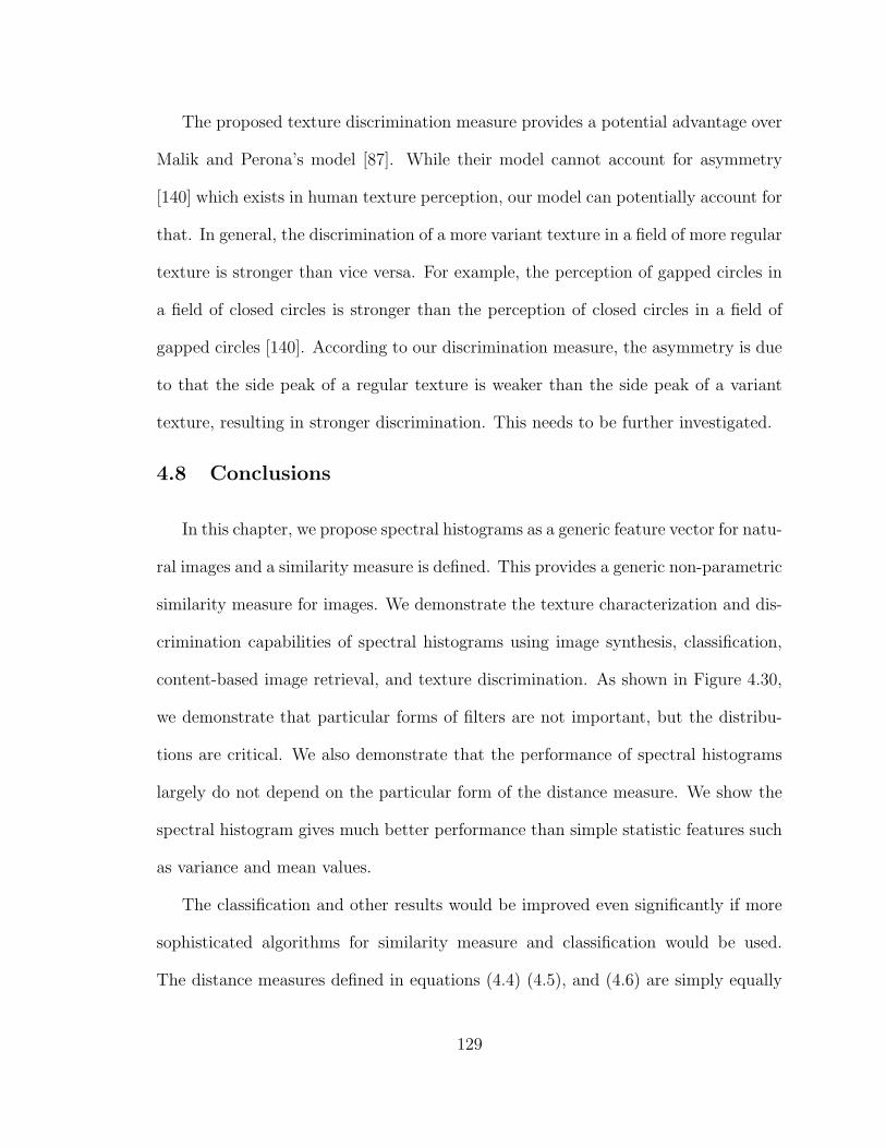
The proposed texture discrimination measure provides a potential advantage over
Malik and Perona’s model [87]. While their model cannot account for asymmetry
[140] which exists in human texture perception, our model can potentially account for
that. In general, the discrimination of a more variant texture in a field of more regular
texture is stronger than vice versa. For example, the perception of gapped circles in
a field of closed circles is stronger than the perception of closed circles in a field of
gapped circles [140]. According to our discrimination measure, the asymmetry is due
to that the side peak of a regular texture is weaker than the side peak of a variant
texture, resulting in stronger discrimination. This needs to be further investigated.
4.8 Conclusions
In this chapter, we propose spectral histograms as a generic feature vector for natu-
ral images and a similarity measure is defined. This provides a generic non-parametric
similarity measure for images. We demonstrate the texture characterization and dis-
crimination capabilities of spectral histograms using image synthesis, classification,
content-based image retrieval, and texture discrimination. As shown in Figure 4.30,
we demonstrate that particular forms of filters are not important, but the distribu-
tions are critical. We also demonstrate that the performance of spectral histograms
largely do not depend on the particular form of the distance measure. We show the
spectral histogram gives much better performance than simple statistic features such
as variance and mean values.
The classification and other results would be improved even significantly if more
sophisticated algorithms for similarity measure and classification would be used.
The distance measures defined in equations (4.4) (4.5), and (4.6) are simply equally
129

weighted summations from all the histogram bins. If many samples are available for
one texture type, homogeneity of the texture can be refined using different weights for
different filters and even bins. Those weights can be learned from training samples,
as demonstrated by Zhu et al [149].
While spectral histograms can capture inhomogeneity of texture images, as shown
in texture synthesis examples, they are not able to capture the geometric relationships
among texture elements if spatially the relationships are longer than the filters used.
Modeling the geometric relationships may even be more salient for certain textures
such as textures consisting of regular patterns of similar elements. A level beyond
this filtering needs to be incorporated or a different module might be needed. One
possible way is to allow short-range coupling instead of nearest-neighbor coupling to
overcome the inhomogeneity present in the image. Those issues need to be further
investigated.
130
CHAPTER 5
IMAGE SEGMENTATION USING SPECTRAL
HISTOGRAMS
Image segmentation is a most fundamental problem in computer vision and im-
age understanding. In this chapter, we propose an new energy functional for image
segmentation which requires explicitly a feature and a distance measure for each seg-
mented region. Using the spectral histogram proposed in the Chapter 4, we derive
an iterative and deterministic approximation algorithm for segmentation. We apply
the algorithm to segmenting images under different assumptions.
5.1 Introduction
Image segmentation is the central problem in computer vision, and the perfor-
mance of high-level modules such as recognition critically depend on segmentation
results. Roughly segmentation can be defined as a constrained partition problem.
Each partition, or region, should be as homogeneous as possible and neighboring par-
titions should be as different as possible. Two computational issues can be identified
from the definition. The first issue is to define features to be used and the associated
131

similarity/dissimilarity measure. Given the similarity/dissimilarity measure, the sec-
ond issue is to design a computational procedure to derive a solution for a given input
image.
To address the first issue, one needs to define a feature, which can be a scalar or
vector and a distance measure in the feature space. In the literature, this issue is
not well addressed. For intensity images, mean and variance values are most widely
used, which are closely related to the Gaussian assumption behind many algorithms
[152] [89] [88] [13] [94] [151]. For texture images, many textural features have been
proposed [44] [43] [61] [18] [65] [21] [127] [107]. Those features in general are only
justified through experiments on selected texture images. Comparing with existing
features, spectral histograms provide a well-justified feature vector. As demonstrated
in the previous chapter, the spectral histogram can effectively capture the texture
appearance and has been successfully applied to image modeling and classification.
The second issue has been studied extensively in the literature. Existing methods
can be classified roughly into local algorithms and optimization of a global criterion.
Local algorithms include edge detectors and region growing [152] [89] [88] [13]. While
good experimental results have been obtained, the major difficulty of local algorithms
is that the segmented regions are not guaranteed to be homogeneous. For example,
in region growing, two different regions may be grouped together due to noise and
variations in local areas. Optimization approaches can be further divided as local
and global based on the segmentation criterion. If the criterion only consists of local
terms, such as in pair-wise classification, those approaches may suffer the problem of
local algorithms. The results may critically depend on parameter values such as the
number of regions.
132

For the global optimization, the central problem is to derive an efficient algorithm
to achieve a good solution due to the high dimensionality of the potential solution
space. In this regard, Mumford-Shah energy functional for segmentation [94] given
in (4.1) is representative in that most existing segmentation algorithms are special
cases [92]. As pointed out earlier, the underlying assumption of the solution space is
piece-wise smooth images. However, to give a solution for segmentation, the solution
space f must be piece-wise constant by the definition of segmentation. In this case,
the energy function becomes [94]:
E(Γ) =∑
i
∫ ∫
Ri
(g(x, y)−meanRi(g))2dxdy + ν|Γ|, (5.1)
where
meanRi(g) =
1
|Ri|∫ ∫
Ri
g(x, y)dxdy.
Here |Ri| is the area of region Ri. There are several limitations of the energy functional
(5.1). The feature to be used is limited to the mean value of a region, which is not
sufficient for characterizing regions as demonstrated in the previous chapter and also
may give undesirable solutions when the mean values of two regions are very close.
Another problem is that a result obtained by minimizing the energy functional is
unpredictable in regions which cannot be described by their mean values. Some of
problems are resolved by using a Gaussian model in the Region Competition algorithm
by Zhu and Yuille [151].
In this chapter, we extend the model (5.1) using the spectral histogram and the
associated distance measure. We develop an algorithm which couples the feature de-
tection and segmentation steps together by extracting features based on the currently
133

available segmentation result. We also develop an algorithm which identifies regional
features in homogeneous texture regions automatically.
In Section 5.2 we give a formulation of our segmentation energy functional. Sec-
tion 5.3 describes our segmentation algorithm. Section 5.4 provides experimental
results when features for each region are given manually. Section 5.5 describes an
automated algorithm for detecting features of homogeneous texture regions. Section
5.6 proposes a method for precise texture boundary localization. Section 5.7 discusses
future research questions along this line. Section 5.8 summarizes the chapter.
5.2 Formulation of Energy Functional for Segmentation
Following the notations used in Mumford and Shah [94], let R be a grid defined
on a planar domain and Ri, i = 1, · · · , n be a disjoint subset of R, Γi be the piece-
wise smooth boundary of Ri, and Γ be the union of Γi, i = 1, · · · , n. A feature Fi
is associated with each region Ri, i = 1, · · · , n. We also define R0, which is called
background [135], as
R0 = R− (R1 ∪ · · ·Rn).
Based on the energy functional by Mumford and Shah [94], given an input image
I, we define an energy functional for segmentation as
E(Ri, n) = λR
n∑
i=1
∑
(x,y)∈Ri
D(FRi(x, y),Fi)+λF
n∑
i=1
n∑
j=1
D(Fi,Fj)+λΓ
n∑
i=1
|Γi|−n∑
i=1
|Ri|.
(5.2)
Here D is a distance measure between a feature at a pixel location and the feature
vector of the region, λR, λF , and λΓ are weights that control the relative contributions
of the corresponding terms.
134

The functional given in (5.2) is motivated by a special case of the functional
by Mumford and Shah [94], as shown in (5.1). In (5.2), the first term encodes the
homogeneity requirement in each region Ri and the second term requires that the
features of the regions should be as different as possible. Here we allow Ri to consist
of several connected regions and we drop the requirement of neighboring regions in
the second term. Alternatively, we can require that each region must be a connected
region and only include neighboring regions in the second term.
The third term requires that boundaries of regions should be as short as possible,
or as smooth as possible. The last term is motivated by the fact that some regions
may not be described well by the selected features. In that case, those regions should
not be labeled as segmented regions. Rather, those regions should be treated as
background, which can be viewed as grouping through inhomogeneity. To illustrate
the motivations, Figure 5.1 shows an intensity image where two regions have similar
mean values but different variances. If we use mean values as features, we argue that
the most reasonable output should be one homogeneous region and another region
which can not be described by the current model. We will discuss this issue later for
segmentation at different scales.
5.3 Algorithms for Segmentation
Given the energy functional defined in (5.2), now the question is to compute a good
solution for a given image. Obviously, due to high dimensionality of the problem, it
is computationally not possible to achieve a good solution by search in the potential
solution space.
135

Figure 5.1: Gray-level image with two regions with similar means but different vari-ances.
Based on different assumptions, we derive approximate solutions. A simple case
is that feature vectors Fi are given. In this case, the problem becomes supervised
classification/segmentation problem. For pixels within a homogeneous region, the
label should be determined based on the minimum distance classifier, which minimizes
the first term in (5.2). For pixels near boundaries between different regions, the
boundary term plays an additional role besides the distance from each feature vector.
Pixels that cannot be classified well by any given feature vector should be labeled as
the background.
Another case is that seed points are given. In this case, the minimization of the
energy functional essentially can be achieved through a procedure similar to region
growing, as demonstrated in [151]. An iterative algorithm can be used by alternating
feature estimation and region growing [151]. In the feature estimation phase, we fix
the segmentation results Ri and estimate Fi by minimizing the energy functional.
The region growing phase is same as the procedure for the case where feature vectors
Fi are given. This case is a generalization of region growing algorithms.
136
The most difficult case is to automatically identify suitable feature vectors for a
given input image and derive a solution. If we could solve this problem, we could
essentially solve the segmentation problem. In this chapter, we develop an algorithm
to automatically identify features from an input image based on the relationships
between different scales and neighboring regions.
Another problem is how to estimate the feature at a given pixel. A straightforward
way is to use a window centered at the pixel always. Another way is to utilize
the currently available results and use asymmetric windows. This helps to further
minimize the boundary uncertainty [151].
In this chapter, we use an iterative but deterministic algorithm. We assume that
the feature vectors for regions, which may be given manually or detected automati-
cally, are close to the true region vectors. In other words, we do not do the feature
re-estimation along the iterations. The first step prior to iterative segmentation is a
minimum distance classifier which generates initial segmentation results. For a given
pixel (x, y) to be updated, we first estimate the spectral histogram using asymmetric
windows around the pixel. Figure 5.2 gives two examples. For simplicity, we use
square windows throughout this chapter, which, in general, give good results but the
biases due the square shapes are visible in several cases. Circular windows provide
better approximation for arbitrary shaped boundaries and are more biologically plau-
sible. In addition, there are many possible choices for windows and the influence of
different choices will be studied in the future.
Because there are several windows to choose at pixel (x, y), for each Fi, we use
the window that has the most number of labels of Ri, and thus the feature at pixel
(x, y) for different labels can be different. We use spectral histograms as features
137

(a) (b)
Figure 5.2: Examples of asymmetric windows. The solid cross is the central pixel.(a) Square windows. (b) Circular windows.
vectors, i.e., FRi(x, y) = H
W(s)
(x,y)
, where W(s)(x,y) is a local neighborhood, the size and
shape of which are given by integration scale W (s) for segmentation. W (s) is a pre-
defined neighborhood. We use χ2-statistic as the distance measure. However, this
distance measure may not provide an accurate measure close to boundaries due to
the inhomogeneity. For example, in the image shown in Figure 5.1, the left region
is homogeneous and the variations allowed should be small. In the right region, the
variations allowed should be relatively large. To overcome this problem and provide
an accurate model, we estimate a probability model of the χ2-statistic for each given
feature vector Fi from the initial classification result. The implementation details
and an example are given in the next section. We approximate the boundary term
by a local term, which is given by the percentage of pixels belonging to the region in
a pre-defined neighborhood. Finally, the local updating rule at pixel (x, y) is given
πi(x, y) = (1−λΓ)P (χ2(HW
(s)
(x,y)
, Hi))+λΓ
∑
(x1,y1)∈N(x,y)
(L(x1, y1) == i)/|N(x, y|. (5.3)
Here L(x, y) is the current region label of pixel (x, y). N(x, y) is a user-defined
neighborhood, and the eight nearest neighbors are used, and λB is a parameter that
138
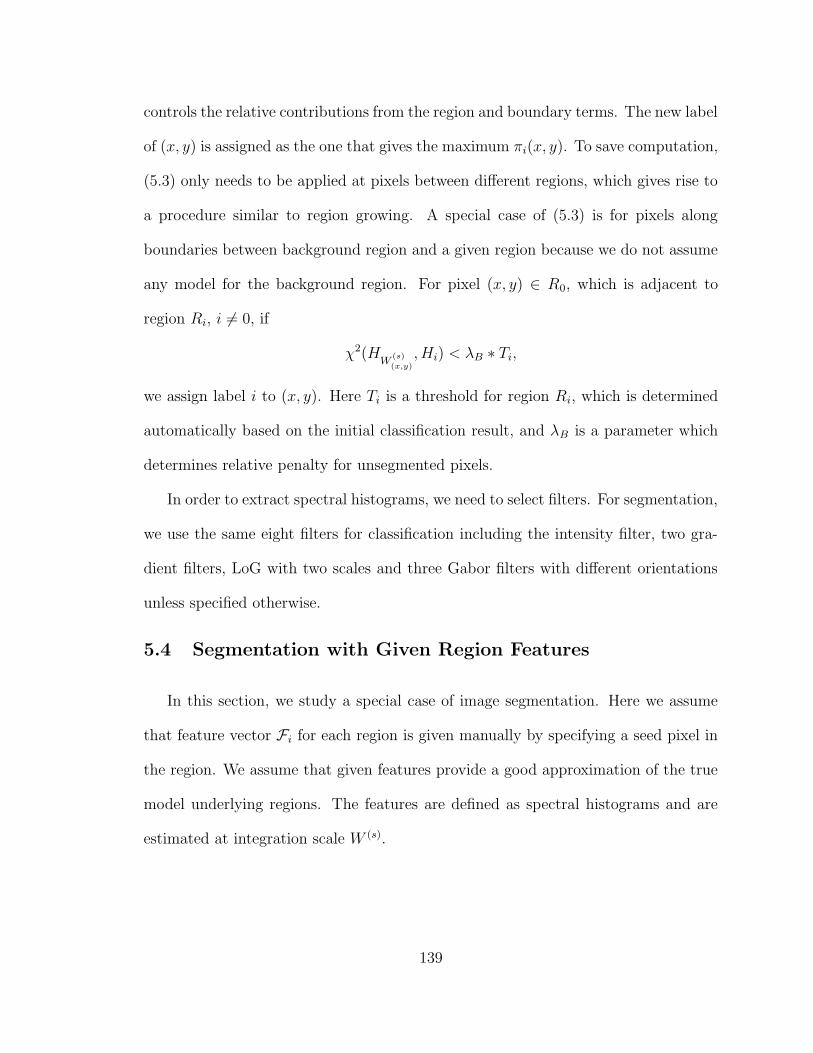
controls the relative contributions from the region and boundary terms. The new label
of (x, y) is assigned as the one that gives the maximum πi(x, y). To save computation,
(5.3) only needs to be applied at pixels between different regions, which gives rise to
a procedure similar to region growing. A special case of (5.3) is for pixels along
boundaries between background region and a given region because we do not assume
any model for the background region. For pixel (x, y) ∈ R0, which is adjacent to
region Ri, i 6= 0, if
χ2(HW
(s)
(x,y)
, Hi) < λB ∗ Ti,
we assign label i to (x, y). Here Ti is a threshold for region Ri, which is determined
automatically based on the initial classification result, and λB is a parameter which
determines relative penalty for unsegmented pixels.
In order to extract spectral histograms, we need to select filters. For segmentation,
we use the same eight filters for classification including the intensity filter, two gra-
dient filters, LoG with two scales and three Gabor filters with different orientations
unless specified otherwise.
5.4 Segmentation with Given Region Features
In this section, we study a special case of image segmentation. Here we assume
that feature vector Fi for each region is given manually by specifying a seed pixel in
the region. We assume that given features provide a good approximation of the true
model underlying regions. The features are defined as spectral histograms and are
estimated at integration scale W (s).
139

5.4.1 Segmentation at a Fixed Integration Scale
First feature vectors Fi are extracted from windows centered at given pixel lo-
cations, the size of which is specified by integration scale W (s). Then the image is
classified using feature vectors Fi, and the classification result is used as the initial
segmentation. To save computation, the initial result is generated by sub-sampling
the input image. To obtain parameters Ti and estimate a probability model, we
compute the histograms of the χ2-statistic between the computed and given spectral
histograms, which are shown in Figure 5.4(b) for the image shown in Figure 5.3(a).
Parameter Ti is determined by the first trough after the first peak from its histogram.
Based on the assumption that feature vectors Fi are close to the true feature vectors,
we derive a probability model by assigning zero probability for values larger than Ti.
The derived probability models are shown in Figure 5.4(b).
To illustrate the effectiveness of using the derived probability model and asym-
metric windows, Figure 5.5(a) shows a row from the image shown in Figure 5.3(a).
Figure 5.5(b) shows the probability of the two labels at each pixel using asymmetric
windows. Here we can see that the edge point is localized precisely at the true loca-
tion. Figure 5.5(c) show the probability using windows centered at pixels. There is an
interval where labels can not be decided because the spectral histogram computed in
the interval does not belong to either of the regions. This shows that the probability
model is sensitive. For comparison, Figure 5.6 shows the results using χ2-statistic
directly. In both asymmetric and central windows cases, the decision boundaries are
not sharp and edge points cannot be localized accurately.
Then the initial segmentation result is refined through an iterative procedure sim-
ilar to region growing but with fixed region features. Due to that spectral histograms
140

(a) (b) (c)
Figure 5.3: Gray-level image segmentation using spectral histograms. The integrationscale W (s) for spectral histograms is a 15× 15 square window, λΓ = 0.2, and λB = 3.Two features are given at (32, 64) and (96, 64). (a) A synthetic image with size128×128. The image is generated by adding zero-mean Gaussian noise with differentσ’s at left and right regions. (b) Initial classification result. (c) Final segmentationresult. The segmentation error is 0.00 % and all the pixels are segmented correctly.
characterize texture properties well, we obtain good experimental results even with
this simple algorithm. The integration scale for spectral histograms is 15 × 15. Fig-
ure 5.3(b) shows the initial classification result. The final result is shown in Figure
5.3(c), where all the pixels are segmented correctly. Due to that the image consists
of two images with similar mean values but different variances, if we apply nonlin-
ear smoothing algorithms, the segmentation result would be wrong because the only
feature is the mean value after smoothing.
Figure 5.7 shows another example of similar means but different variances. Here
the boundary is ’S’ shaped to test the algorithm for irregular boundaries. Here the
boundary is preserved well but artifacts due to the square windows are evident. Near
top and bottom image borders, the error is the most due to the boundary effects.
Figure 5.8 shows an example with two texture regions. Because the two textures
are relatively homogeneous, the segmentation result is very accurate.
141

0 0.2 0.4 0.6 0.8 1 1.2 1.4 1.6 1.8
0
20
40
60
80
100
120
(a)
0 0.1 0.2 0.3 0.4 0.5 0.6 0.7 0.8−0.05
0
0.05
0.1
0.15
0.2
0.25
0.3
0.35
0.4
0.45
(b)
Figure 5.4: The histogram and derived probability model of χ2-statistic for the givenregion features. Solid lines stand for left region and dashed lines stand for right region.(a) The histogram of the χ2-statistic between the given feature and the computed onesat a coarser grid. (b) The derived probability model for the left and right regions.
142
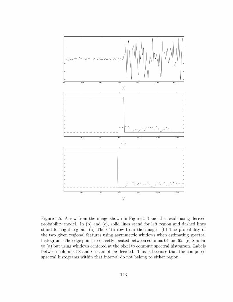
0 20 40 60 80 100 120
(a)
20 40 60 80 100 120
(b)
20 40 60 80 100 120
(c)
Figure 5.5: A row from the image shown in Figure 5.3 and the result using derivedprobability model. In (b) and (c), solid lines stand for left region and dashed linesstand for right region. (a) The 64th row from the image. (b) The probability ofthe two given regional features using asymmetric windows when estimating spectralhistogram. The edge point is correctly located between columns 64 and 65. (c) Similarto (a) but using windows centered at the pixel to compute spectral histogram. Labelsbetween columns 58 and 65 cannot be decided. This is because that the computedspectral histograms within that interval do not belong to either region.
143
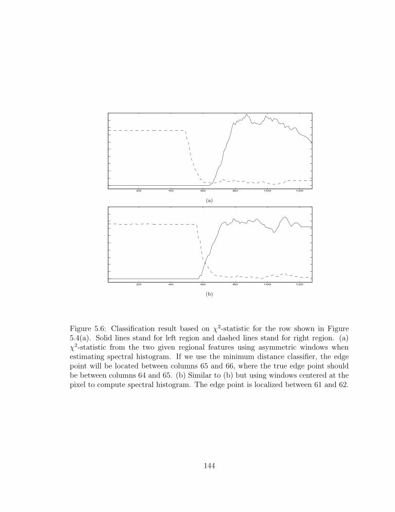
20 40 60 80 100 120
(a)
20 40 60 80 100 120
(b)
Figure 5.6: Classification result based on χ2-statistic for the row shown in Figure5.4(a). Solid lines stand for left region and dashed lines stand for right region. (a)χ2-statistic from the two given regional features using asymmetric windows whenestimating spectral histogram. If we use the minimum distance classifier, the edgepoint will be located between columns 65 and 66, where the true edge point shouldbe between columns 64 and 65. (b) Similar to (b) but using windows centered at thepixel to compute spectral histogram. The edge point is localized between 61 and 62.
144
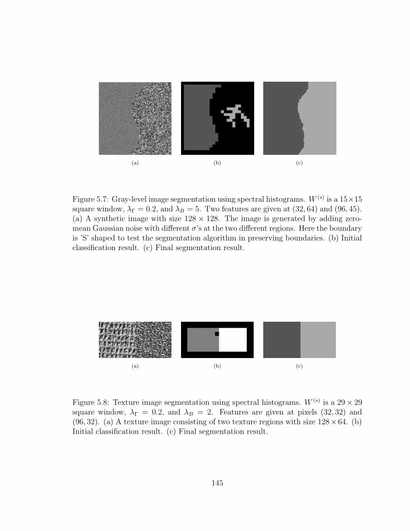
(a) (b) (c)
Figure 5.7: Gray-level image segmentation using spectral histograms. W (s) is a 15×15square window, λΓ = 0.2, and λB = 5. Two features are given at (32, 64) and (96, 45).(a) A synthetic image with size 128 × 128. The image is generated by adding zero-mean Gaussian noise with different σ’s at the two different regions. Here the boundaryis ’S’ shaped to test the segmentation algorithm in preserving boundaries. (b) Initialclassification result. (c) Final segmentation result.
(a) (b) (c)
Figure 5.8: Texture image segmentation using spectral histograms. W (s) is a 29× 29square window, λΓ = 0.2, and λB = 2. Features are given at pixels (32, 32) and(96, 32). (a) A texture image consisting of two texture regions with size 128× 64. (b)Initial classification result. (c) Final segmentation result.
145
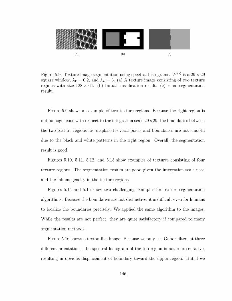
(a) (b) (c)
Figure 5.9: Texture image segmentation using spectral histograms. W (s) is a 29× 29square window, λΓ = 0.2, and λB = 3. (a) A texture image consisting of two textureregions with size 128 × 64. (b) Initial classification result. (c) Final segmentationresult.
Figure 5.9 shows an example of two texture regions. Because the right region is
not homogeneous with respect to the integration scale 29×29, the boundaries between
the two texture regions are displaced several pixels and boundaries are not smooth
due to the black and white patterns in the right region. Overall, the segmentation
result is good.
Figures 5.10, 5.11, 5.12, and 5.13 show examples of textures consisting of four
texture regions. The segmentation results are good given the integration scale used
and the inhomogeneity in the texture regions.
Figures 5.14 and 5.15 show two challenging examples for texture segmentation
algorithms. Because the boundaries are not distinctive, it is difficult even for humans
to localize the boundaries precisely. We applied the same algorithm to the images.
While the results are not perfect, they are quite satisfactory if compared to many
segmentation methods.
Figure 5.16 shows a texton-like image. Because we only use Gabor filters at three
different orientations, the spectral histogram of the top region is not representative,
resulting in obvious displacement of boundary toward the upper region. But if we
146

(a) (b) (c)
Figure 5.10: Texture image segmentation using spectral histograms. W (s) is a 35×35square window, λΓ = 0.4, and λB = 3. Four features are given at (32, 32), (32, 96),(96, 32), and (96, 96). (a) A texture image consisting of four texture regions with size128× 128. (b) Initial classification result. (c) Final segmentation result.
(a) (b) (c)
Figure 5.11: Texture image segmentation using spectral histograms. W (s) is a 35×35square window, λΓ = 0.4, and λB = 3. Four features are given at (32, 32), (32, 96),(96, 32), and (96, 96). (a) A texture image consisting of four texture regions with size128× 128. (b) Initial classification result. (c) Final segmentation result.
147
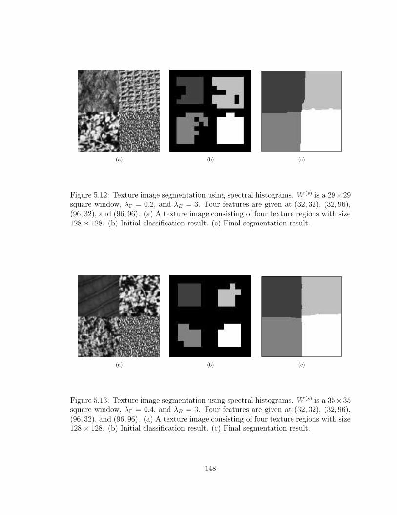
(a) (b) (c)
Figure 5.12: Texture image segmentation using spectral histograms. W (s) is a 29×29square window, λΓ = 0.2, and λB = 3. Four features are given at (32, 32), (32, 96),(96, 32), and (96, 96). (a) A texture image consisting of four texture regions with size128× 128. (b) Initial classification result. (c) Final segmentation result.
(a) (b) (c)
Figure 5.13: Texture image segmentation using spectral histograms. W (s) is a 35×35square window, λΓ = 0.4, and λB = 3. Four features are given at (32, 32), (32, 96),(96, 32), and (96, 96). (a) A texture image consisting of four texture regions with size128× 128. (b) Initial classification result. (c) Final segmentation result.
148

(a) (b) (c)
Figure 5.14: A challenging example for texture image segmentation. W (s) is a 35×35square window, λΓ = 0.4, and λB = 20. Two features are given at (160, 160) and(252, 250). (a) Input image consisting of two texture images, where the boundary cannot be localized clearly because of their similarity. The size of the image is 320× 320in pixels. (b) Initial classification result. (c) Final segmentation result.
(a) (b) (c)
Figure 5.15: Another challenging example for texture segmentation. W (s) is a 35×35square window, λΓ = 0.4, and λB = 20. Two features are given at (160, 160) and(252, 250). (a) Input image consisting of two texture images, where the boundary cannot be localized clearly because of their similarity. The size of the image is 320× 320in pixels. (b) Initial classification result. (c) Final segmentation result.
149
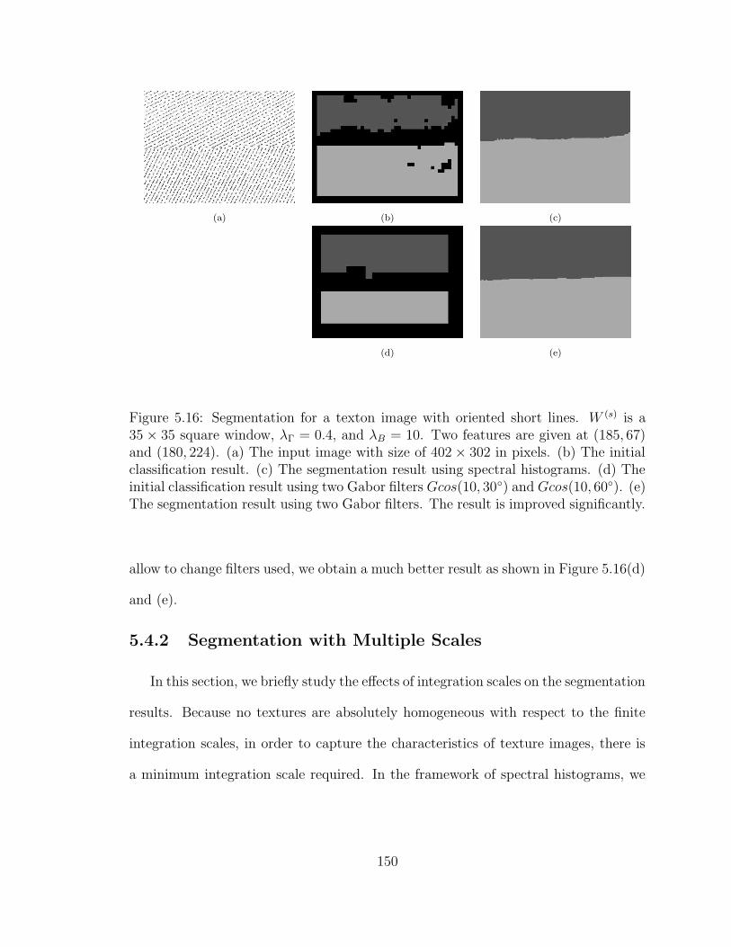
(a) (b) (c)
(d) (e)
Figure 5.16: Segmentation for a texton image with oriented short lines. W (s) is a35 × 35 square window, λΓ = 0.4, and λB = 10. Two features are given at (185, 67)and (180, 224). (a) The input image with size of 402× 302 in pixels. (b) The initialclassification result. (c) The segmentation result using spectral histograms. (d) Theinitial classification result using two Gabor filters Gcos(10, 30) and Gcos(10, 60). (e)The segmentation result using two Gabor filters. The result is improved significantly.
allow to change filters used, we obtain a much better result as shown in Figure 5.16(d)
and (e).
5.4.2 Segmentation with Multiple Scales
In this section, we briefly study the effects of integration scales on the segmentation
results. Because no textures are absolutely homogeneous with respect to the finite
integration scales, in order to capture the characteristics of texture images, there is
a minimum integration scale required. In the framework of spectral histograms, we
150
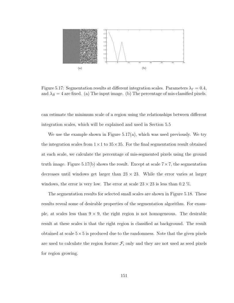
0 5 10 15 20 25 30 350
0.1
0.2
0.3
0.4
0.5
0.6
0.7
0.8
(a) (b)
Figure 5.17: Segmentation results at different integration scales. Parameters λΓ = 0.4,and λB = 4 are fixed. (a) The input image. (b) The percentage of mis-classified pixels.
can estimate the minimum scale of a region using the relationships between different
integration scales, which will be explained and used in Section 5.5
We use the example shown in Figure 5.17(a), which was used previously. We try
the integration scales from 1×1 to 35×35. For the final segmentation result obtained
at each scale, we calculate the percentage of mis-segmented pixels using the ground
truth image. Figure 5.17(b) shows the result. Except at scale 7×7, the segmentation
decreases until windows get larger than 23 × 23. While the error varies at larger
windows, the error is very low. The error at scale 23× 23 is less than 0.2 %.
The segmentation results for selected small scales are shown in Figure 5.18. These
results reveal some of desirable properties of the segmentation algorithm. For exam-
ple, at scales less than 9 × 9, the right region is not homogeneous. The desirable
result at these scales is that the right region is classified as background. The result
obtained at scale 5×5 is produced due to the randomness. Note that the given pixels
are used to calculate the region feature Fi only and they are not used as seed pixels
for region growing.
151

(a) (b)
(c) (d)
Figure 5.18: Segmentation results using different segmentation scales for the imageshown in Figure 5.17(a). In each sub-figure, the left shows the initial classificationresult and the right shows the segmentation result. Parameters λΓ = 0.4, and λB = 4are fixed. (a) W (s) is a 1× 1 square window. (b) W (s) is a 3× 3 square window. (c)W (s) is a 5× 5 square window. (d) W (s) is a 7× 7 square window.
152

5.4.3 Region-of-interest Extraction
Here we try to segment natural texture images. Because natural images consist
many regions that are not homogeneous texture regions, we segment regions that are
specified through region features. For each image, we only give one region feature
and the algorithm is essentially to segment region of interest. As mentioned before,
in our algorithm, no assumption is made regarding the distributions and properties
of the background regions.
We apply the same algorithm. Figure 5.19 shows the result for a cheetah image. If
we use the same filters, the initial result is shown in Figure 5.19(b) and the segmenta-
tion result is shown in Figure 5.19(c). Here the boundaries are not localized well due
to the similarity between the surrounding areas and the white part of cheetah skin.
The tail is not included because that area is relatively dark. If we do not use the
intensity filter and use gradient and LoG filters, the tail is then correctly segmented
as shown in Figure 5.19(e). If we have a database for recognition, the cheetah can
be easily recognized due to its distinctive skin pattern which is characterized by its
spectral histograms.
Figure 5.20 shows an indoor image which includes a sofa with texture surface.
Figure 5.20(c) shows the final result. The lower boundary of the sofa is localized well
due to that the floors are different from the sofa texture. However, the boundaries
of top and right part are not localized well due to that the intensity values at those
regions are similar to the white part of sofa texture. If we put another regional
feature in the white area, the top boundary can be localized more accurately through
competition as shown in Figure 5.20(d).
153
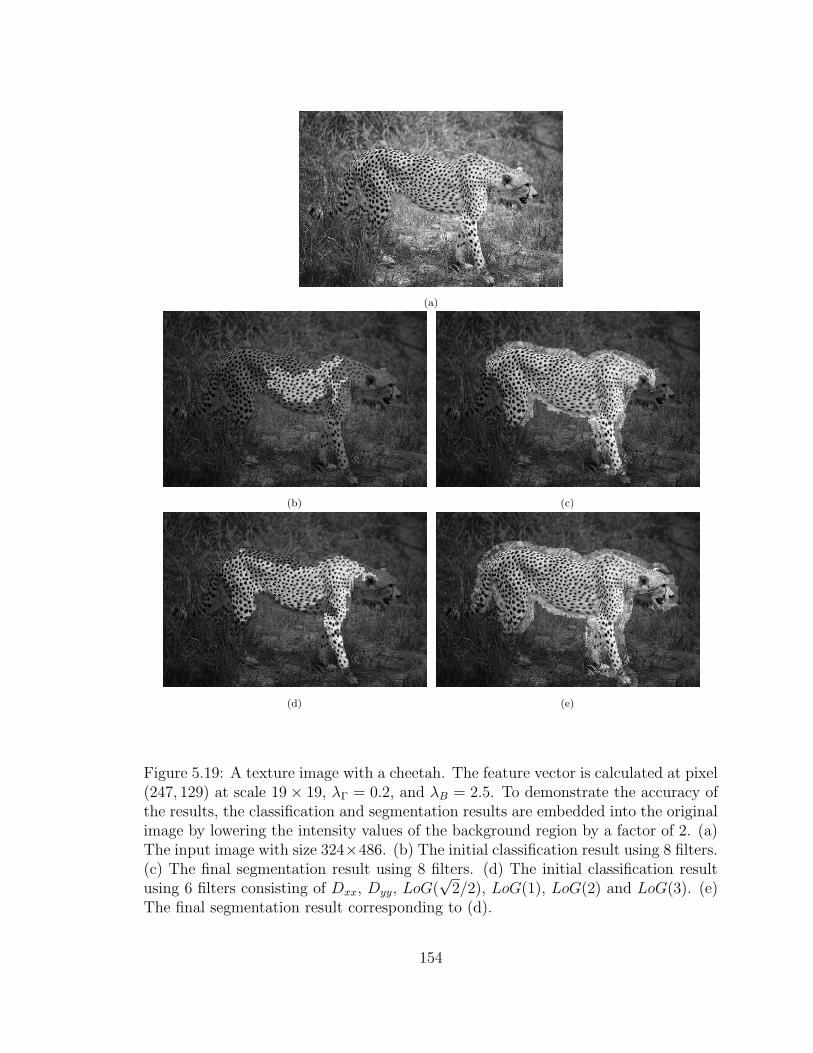
(a)
(b) (c)
(d) (e)
Figure 5.19: A texture image with a cheetah. The feature vector is calculated at pixel(247, 129) at scale 19× 19, λΓ = 0.2, and λB = 2.5. To demonstrate the accuracy ofthe results, the classification and segmentation results are embedded into the originalimage by lowering the intensity values of the background region by a factor of 2. (a)The input image with size 324×486. (b) The initial classification result using 8 filters.(c) The final segmentation result using 8 filters. (d) The initial classification resultusing 6 filters consisting of Dxx, Dyy, LoG(
√2/2), LoG(1), LoG(2) and LoG(3). (e)
The final segmentation result corresponding to (d).
154

(a) (b)
(c) (d)
Figure 5.20: An indoor image with a sofa. The feature vector is calculated at pixel(146, 169) at scale 35×35, λΓ = 0.2, and λB = 3. (a) Input image with size 512×512.(b) Initial classification result. (c) Final segmentation result. (d) Segmentation resultif we assume there is another region feature given at (223, 38).
155
5.5 Automated Seed Selection
In the segmentation experiments presented above, we assume that several rep-
resentative pixels are given. Those pixels are used to calculate feature vectors of
the corresponding regions. This assumption is obviously too restrictive for an au-
tonomous system. Also the human visual system does not need this assumption but
can deal with a wide range of texture images robustly and reliably. In this section,
we attempt to develop a solution for identifying seed points automatically in an input
image. The proposed method is based on the spectral histogram and is consistent
with the proposed computational framework.
The basic idea under the proposed method is to identify homogeneous texture
regions within a given image. As discussed in the previous chapter, the spectral his-
togram can be defined on image patches with different sizes and shapes and those
spectral histograms defined on different patches can still be compared using the sim-
ilarity/dissimilarity measure as spectral histograms are naturally normalized.
We try to identify homogeneous texture regions based on the divergence between
two integration scales. Let W (a) be an integration scale larger than W (s), the integra-
tion scale for segmentation, we define the distance between the two scales centered
at pixel (x, y)
ψ(s,a)(x, y) = D(HW (s)(x,y), HW (a)(x,y)). (5.4)
Within a homogeneously defined texture region, ψ(s,a) should be small because
HW (s)(x, y) and HW (a)
(x, y) should be similar. We also define a distance measure
156
between different windows at scale W (s) within the window given by W (a),
ψ(s,s)(x, y) = maxW (s)(x1, y1) ⊂ W (a)(x, y)W (s)(x2, y2) ⊂ W (a)(x, y)
D(HW (s)(x1,y1), HW (s)(x2,y2)). (5.5)
Equation (5.5) is approximated at implementation using central and four corner
windows within W (a). Finally, we want to choose features that are as different as
possible from those already chosen. Suppose we choose n features already, where,
Fi = HW (s)(x,y), for i = 1, . . . , n, we define
ψ(c)(x, y) = max1≤i≤n
D(HW (s)(x,y),Fi). (5.6)
We have the following saliency measure
ψ(x, y) = (1− λC)(λA×ψ(s,a)(x, y) + (1− λA)×ψ(s,s)(x, y))− λC ×ψ(c)(x, y). (5.7)
Here λA and λC are parameters to determine the relative contribution of each term.
To save computation, we compute ψ(x, y) on a coarser grid. Feature vectors are
chosen according to the value of ψ(x, y) until
λA × ψ(s,a)(x, y) + (1− λA)× ψ(s,s)(x, y) < TA,
where TA is a threshold.
Figures 5.21-5.25 show the segmentation results for texture images. Here the algo-
rithm identifies the feature vectors automatically instead of manually chosen features.
Due to the inhomogeneity, some of texture boundaries are not as good as the results
with the manually given feature points. This is due to that the windows for feature
selection are large compared to the texture regions.
157

(a) (b) (c)
Figure 5.21: Texture image segmentation with representative pixels identified au-tomatically. W (s) is a 29 × 29 square window, W (a) is a 35 × 35 square window,λC = 0.1, λA = 0.2, λB = 2.0, λΓ = 0.2, and TA = 0.08. (a) Input texture image,which is shown in Figure 5.8. (b) Initial classification result. Here the representativepixels are detected automatically. (c) Final segmentation result.
(a) (b) (c)
Figure 5.22: Texture image segmentation with representative pixels identified au-tomatically. W (s) is a 29 × 29 square window, W (a) is a 43 × 43 square window,λC = 0.4, λA = 0.4, λB = 5.0, λΓ = 0.4, and TA = 0.30. (a) Input texture image,which is shown in Figure 5.10. (b) Initial classification result. Here the representativepixels are detected automatically. (c) Final segmentation result.
158

(a) (b) (c)
Figure 5.23: Texture image segmentation with representative pixels identified au-tomatically. W (s) is a 29 × 29 square window, W (a) is a 43 × 43 square window,λC = 0.1, λA = 0.2, λB = 5.0, λΓ = 0.4, and TA = 0.20. (a) Input texture image,which is shown in Figure 5.11. (b) Initial classification result. Here the representativepixels are detected automatically. (c) Final segmentation result.
(a) (b) (c)
W (s) is a 29×29 square window, W (a) is a 43×43 square window, λC = 0.1, λA = 0.2,λB = 5.0, λΓ = 0.4, and TA = 0.20.
Figure 5.24: Texture image segmentation with representative pixels identified au-tomatically. (a) Input texture image, which is shown in Figure 5.12. (b) Initialclassification result. Here the representative pixels are detected automatically. (c)Final segmentation result.
159

(a) (b) (c)
Figure 5.25: Texture image segmentation with representative pixels identified auto-matically. W (s) is a 29×29 square window, W (a) is a 43×43 square window, λC = 0.1,λA = 0.2, λB = 5.0, λΓ = 0.4, and TA = 0.20. (a) Input texture image, which is shownin Figure 5.13. Here the representative pixels are detected automatically. (c) Finalsegmentation result.
5.6 Localization of Texture Boundaries
Because textures need to be characterized by spatial relationships among pix-
els, relatively large integration windows are needed in order to extract meaningful
features, which is evident from Figure 4.23(b), which shows that the classification
performance degrades dramatically when the integration scale gets too small. The
large integration scale we use results in large errors along texture boundaries due to
the uncertainty introduced by large windows [13]. By using asymmetric windows for
feature extraction, the uncertainty effect is reduced. However, for arbitrary texture
boundaries, the errors along boundaries can be large even when the overall segmen-
tation performance is good. For example, Figure 5.26(b) shows a segmentation result
using spectral histograms. While the segmentation error is only 6.55%, visually the
160
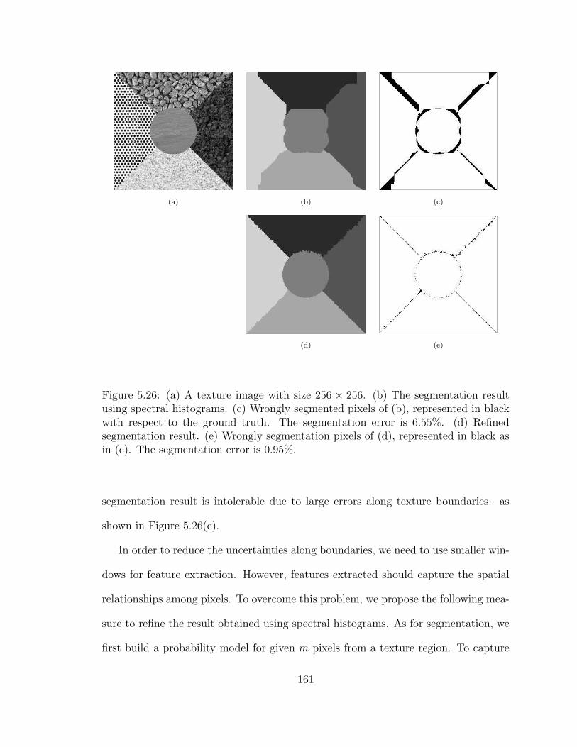
(a) (b) (c)
(d) (e)
Figure 5.26: (a) A texture image with size 256 × 256. (b) The segmentation resultusing spectral histograms. (c) Wrongly segmented pixels of (b), represented in blackwith respect to the ground truth. The segmentation error is 6.55%. (d) Refinedsegmentation result. (e) Wrongly segmentation pixels of (d), represented in black asin (c). The segmentation error is 0.95%.
segmentation result is intolerable due to large errors along texture boundaries. as
shown in Figure 5.26(c).
In order to reduce the uncertainties along boundaries, we need to use smaller win-
dows for feature extraction. However, features extracted should capture the spatial
relationships among pixels. To overcome this problem, we propose the following mea-
sure to refine the result obtained using spectral histograms. As for segmentation, we
first build a probability model for given m pixels from a texture region. To capture
161
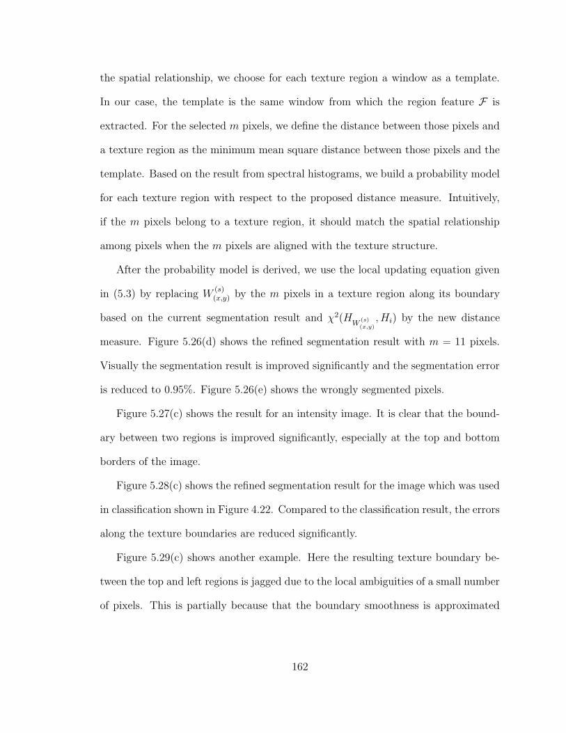
the spatial relationship, we choose for each texture region a window as a template.
In our case, the template is the same window from which the region feature F is
extracted. For the selected m pixels, we define the distance between those pixels and
a texture region as the minimum mean square distance between those pixels and the
template. Based on the result from spectral histograms, we build a probability model
for each texture region with respect to the proposed distance measure. Intuitively,
if the m pixels belong to a texture region, it should match the spatial relationship
among pixels when the m pixels are aligned with the texture structure.
After the probability model is derived, we use the local updating equation given
in (5.3) by replacing W(s)(x,y) by the m pixels in a texture region along its boundary
based on the current segmentation result and χ2(HW
(s)
(x,y)
, Hi) by the new distance
measure. Figure 5.26(d) shows the refined segmentation result with m = 11 pixels.
Visually the segmentation result is improved significantly and the segmentation error
is reduced to 0.95%. Figure 5.26(e) shows the wrongly segmented pixels.
Figure 5.27(c) shows the result for an intensity image. It is clear that the bound-
ary between two regions is improved significantly, especially at the top and bottom
borders of the image.
Figure 5.28(c) shows the refined segmentation result for the image which was used
in classification shown in Figure 4.22. Compared to the classification result, the errors
along the texture boundaries are reduced significantly.
Figure 5.29(c) shows another example. Here the resulting texture boundary be-
tween the top and left regions is jagged due to the local ambiguities of a small number
of pixels. This is partially because that the boundary smoothness is approximated
162

(a) (b) (c)
Figure 5.27: (a) A synthetic image with size 128 × 128, as shown in Figure 5.7(a).(b) The segmentation result using spectral histograms as shown in Figure 5.7(c). (c)Refined segmentation result.
Figure 5.28: (a) A texture image with size 256 × 256. (b) The segmentation resultusing spectral histograms. (c) Refined segmentation result.
163
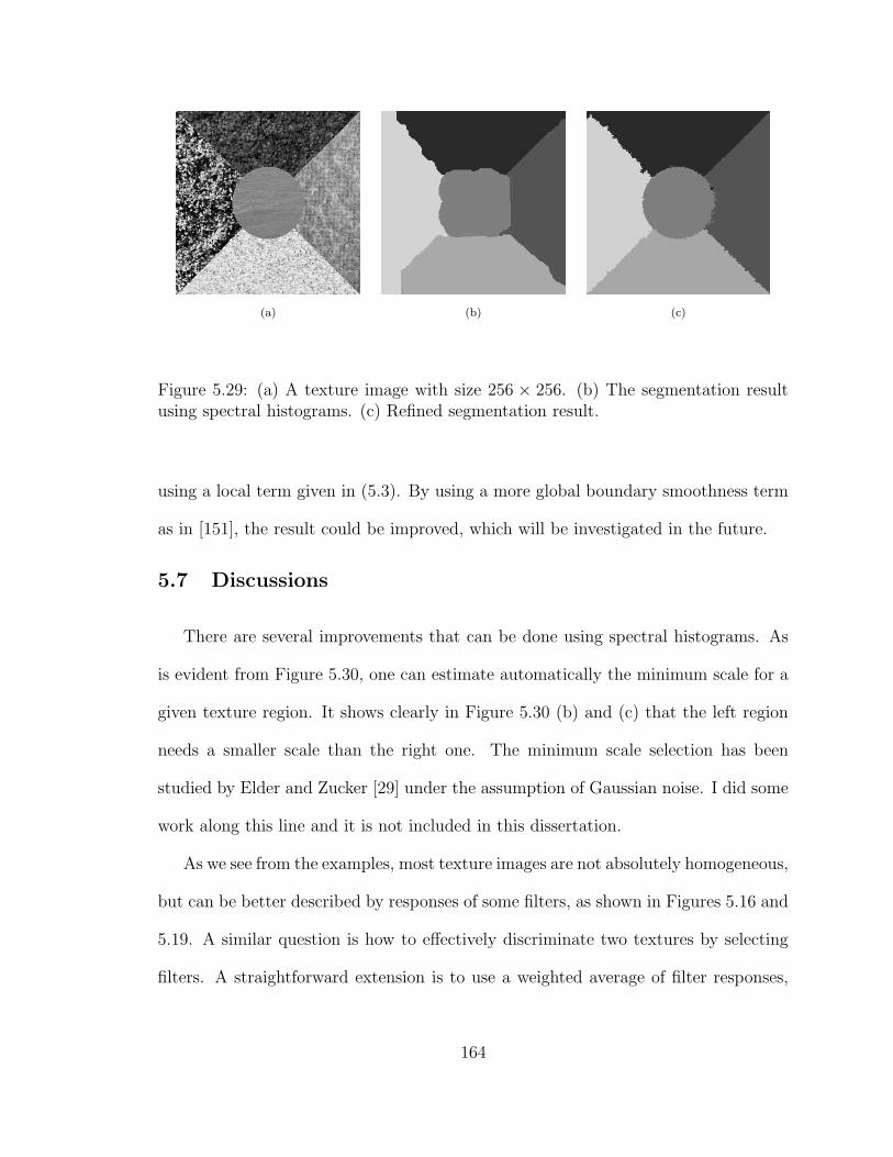
(a) (b) (c)
Figure 5.29: (a) A texture image with size 256 × 256. (b) The segmentation resultusing spectral histograms. (c) Refined segmentation result.
using a local term given in (5.3). By using a more global boundary smoothness term
as in [151], the result could be improved, which will be investigated in the future.
5.7 Discussions
There are several improvements that can be done using spectral histograms. As
is evident from Figure 5.30, one can estimate automatically the minimum scale for a
given texture region. It shows clearly in Figure 5.30 (b) and (c) that the left region
needs a smaller scale than the right one. The minimum scale selection has been
studied by Elder and Zucker [29] under the assumption of Gaussian noise. I did some
work along this line and it is not included in this dissertation.
As we see from the examples, most texture images are not absolutely homogeneous,
but can be better described by responses of some filters, as shown in Figures 5.16 and
5.19. A similar question is how to effectively discriminate two textures by selecting
filters. A straightforward extension is to use a weighted average of filter responses,
164
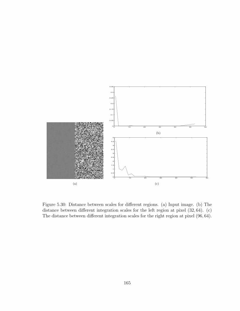
0 10 20 30 40 50 600
0.05
0.1
0.15
0.2
0.25
0.3
0.35
(b)
0 10 20 30 40 50 600
0.5
1
1.5
2
2.5
3
3.5
4
4.5
5
(a) (c)
Figure 5.30: Distance between scales for different regions. (a) Input image. (b) Thedistance between different integration scales for the left region at pixel (32, 64). (c)The distance between different integration scales for the right region at pixel (96, 64).
165
as in the FRAME model [149] [150]
χ2(HI1 , HI2) =K∑
α=1
∑
z
λ(α)z
(H(α)I1
(z)−H(α)I2
(z))2
H(α)I1
(z) +H(α)I2
(z). (5.8)
There are two issues here. If we have training samples available, we can use param-
eter estimation methods [149] [150]. We can also use a neural network to learn the
weights. For image segmentation, the main problem is how we can obtain training
samples along the segmentation procedure. One way is to use the initial segmenta-
tion result. The other way is to alternate between two phases. In the training phase,
we can re-estimate the parameters using the current segmentation result and in the
segmentation phase we can use the current parameters for segmentation.
Some of textures cannot be captured well using spectral histograms when the fil-
ter responses are not homogeneous. Rather, the spatial relationships among texture
elements are more prominent. For the example, the zebra stripes shown in Figure
5.31(a) cannot be captured well using spectral histograms, especially the boundaries
are not localized well. Given that the surrounding area is close to the white part of
zebra stripes and zebra stripes are not homogeneous, the result is what one would
expect using a homogeneous model. No matter what homogeneity measure is used,
it would not work well in cases like the zebra image because the zebra stripes are
simply not homogeneous. To overcome this problem, one needs to define a model
which can characterize the structural relationships in a generic way. Within the spa-
tial/frequency representational framework, short-range order coupling may provide a
solution. In other words, the filter responses capture the local shape information and
short-range order coupling overcomes the inhomogeneity in the region. This may lead
to a new computational model and needs to be further investigated and studied.
166
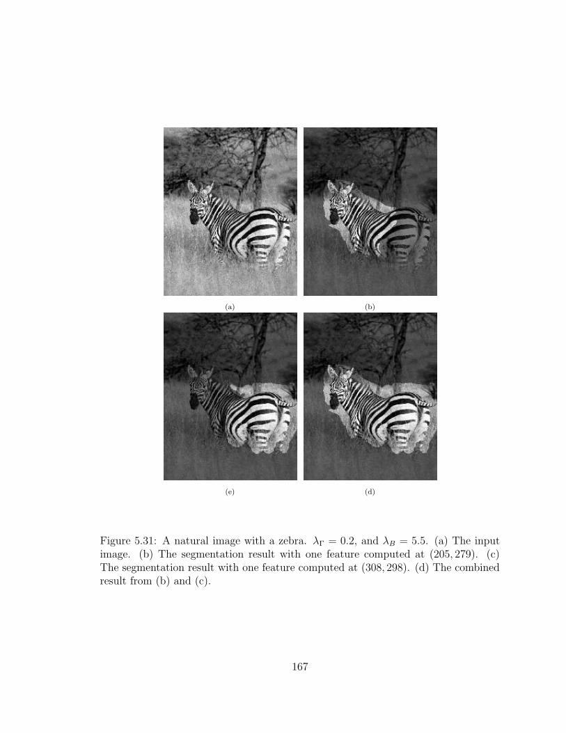
(a) (b)
(e) (d)
Figure 5.31: A natural image with a zebra. λΓ = 0.2, and λB = 5.5. (a) The inputimage. (b) The segmentation result with one feature computed at (205, 279). (c)The segmentation result with one feature computed at (308, 298). (d) The combinedresult from (b) and (c).
167

5.8 Conclusions
In this chapter, we formulate an energy functional for image segmentation by
making features and homogeneity measures explicit for segmented regions. We have
developed a segmentation algorithm using spectral histograms as a generic feature for
natural images and χ2-statistic as a similarity measure. We investigate the perfor-
mance of the algorithms under different assumptions. Satisfactory results have been
obtained using intensity, texture, and natural images. Future work along this line is
discussed.
168

CHAPTER 6
PERCEPTUAL ORGANIZATION BASED ON
TEMPORAL DYNAMICS
This chapter presents a computational model for perceptual organization. A
figure-ground segregation network is proposed based on a novel boundary pair rep-
resentation. Nodes in the network are boundary segments obtained through local
grouping. Each node is excitatorily coupled with the neighboring nodes that belong
to the same region, and inhibitorily coupled with the corresponding paired node. The
status of a node represents the probability of the node being figural and is updated
according to a differential equation. The system solves the figure-ground segregation
problem through temporal evolution. Gestalt-like grouping rules are incorporated
by modulating connections, which determines the temporal behavior and thus the
perception of the system. The results are then fed to a surface completion module
based on local diffusion. Different perceptual phenomena, such as modal and amodal
completion, virtual contours, grouping and shape decomposition are explained by the
model with a fixed set of parameters. Computationally, the system eliminates combi-
natorial optimization, which is common to many existing computational approaches.
It also accounts for more examples that are consistent with psychological experiments.
In addition, the boundary-pair representation is consistent with well-known on- and
169
off-center cell responses and thus biologically more plausible. The results appear in
[81] [82].
6.1 Introduction
Perceptual organization refers to the ability of grouping similar features in sen-
sory data. This, at a minimum, includes the operations of grouping and figure-ground
segregation. Here grouping includes both local grouping, generally known as segmen-
tation, and long-range grouping, referred to as perceptual grouping in this chapter.
Figure-ground segregation refers to the process of determining the relative depth of
adjacent regions in the input.
This problem setting has several computational implications. The central problem
in perceptual organization is figure-ground segregation. When the relative depth
between regions is determined, different types of surface completion phenomena, such
as modal and amodal completion, shape composition and perceptual grouping, can be
solved and explained using a single framework. Perceptual grouping can be inferred
from surface completion. Grouping rules, such as those summarized by Gestaltists,
can be incorporated for figure-ground segregation.
Many computational models have been proposed for perceptual organization.
Many of the existing approaches [86] [41] [98] [141] [34] start from detecting dis-
continuities i.e. edges in the input; one or several configurations are then selected
according to certain criteria, for example, non-accidentalness [86]. Those approaches
to a larger extend are influenced by Marr’s paradigm [88], which is supported by that
on- and off-center cells response to luminance differences, or edges [53], and that the
three-dimensional shapes of the parts can be inferred from a two-dimensional line
170
drawing [7]. While those approaches work well to derive meaningful two-dimensional
regions and their boundaries, there are several disadvantages for perceptual organi-
zation. Theoretically speaking, edges should be localized between regions and do
not belong to any region. By detecting and using edges from the input, an addi-
tional ambiguity, the ownership of a boundary segment, is introduced. Ownership
problem is equivalent to figure-ground segregation [97]. Due to that, regional attri-
butions cannot be associated with boundary segments. Further more, because each
boundary segment can belong to different regions, the potential search space is com-
binatorial; constraints among different segments such as topological constraints must
be incorporated explicitly [141]. Furthermore, obtaining the optimal configuration(s)
is computationally expensive.
To overcome some of the problems, we propose a laterally-coupled network based
on a boundary-pair representation. An occluding boundary is represented by a pair
of boundaries of the two involved regions, and initiates a competition between the
regions. Each node in the network represents a boundary segment. A closed region
boundary is represented as a ring structure with laterally coupled nodes. A region
consists of one or more rings. Regions compete to be figural through boundary-pair
competition and the figure-ground segregation is solved through temporal evolution.
Gestalt grouping rules are incorporated by modulating the coupling strength be-
tween different nodes within a region, which influences the temporal dynamics and
determines the perception of the system. Shape decomposition and grouping are im-
plemented through local diffusion using the results from figure-ground segregation.
This approach offers several advantages over edge-based approaches:
171
• Boundary-pair representation makes explicit the ownership of boundary seg-
ments and eliminates the combinatorial optimization necessary for many exist-
ing approaches.
• The model can explain more perceptual phenomena than existing approaches
using a fixed set of parameters.
• It can incorporate top-down influence naturally.
In Section 6.2 we introduce figure-ground segregation network and demonstrate
the temporal properties of the network. Section 6.3 shows how surface completion
and decomposition are achieved. Section 6.4 provides experimental results. Section
6.5 concludes the chapter with further discussions.
6.2 Figure-Ground Segregation Network
The central problem in perceptual organization is to determine the relative depth
among regions. As figural reversal occurs in certain circumstances, figure-ground
segregation cannot be resolved only based on local attributes. By using a boundary-
pair representation, the solution to figure-ground segregation is given by temporal
evolution.
6.2.1 Boundary-Pair Representation
The boundary-pair representation is motivated by on- and off-center cell responses.
Figure 6.1(a) shows an input image. Figure 6.1(b) and (c) show the on-center and
off-center responses. Without zero-crossing, we naturally obtain double responses for
each occluding boundary, as shown in Figure 6.1(d).
172
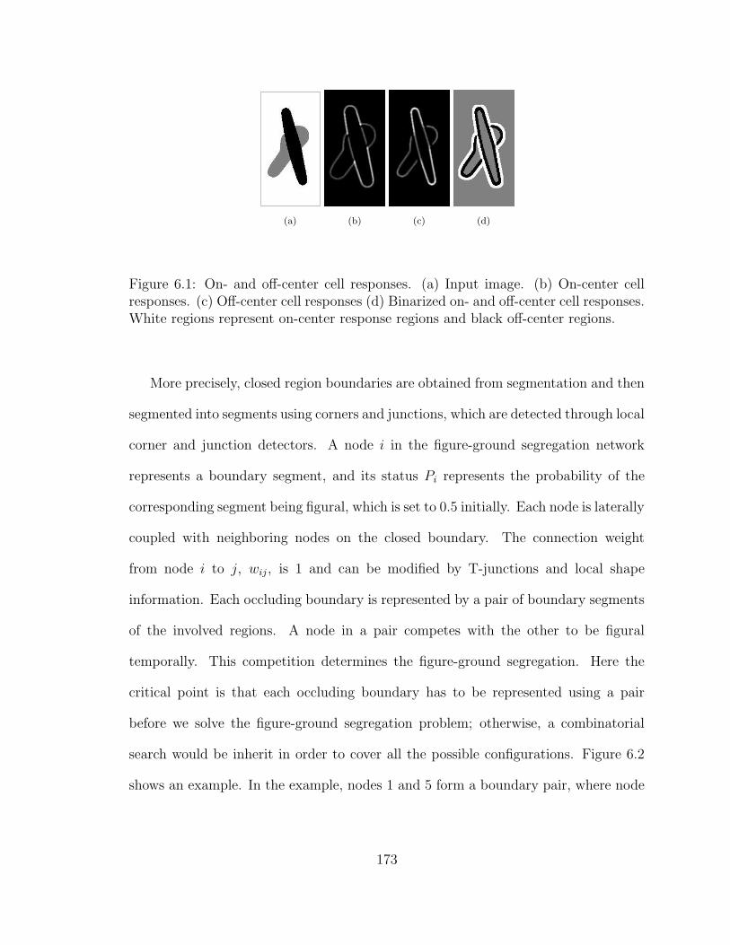
(a) (b) (c) (d)
Figure 6.1: On- and off-center cell responses. (a) Input image. (b) On-center cellresponses. (c) Off-center cell responses (d) Binarized on- and off-center cell responses.White regions represent on-center response regions and black off-center regions.
More precisely, closed region boundaries are obtained from segmentation and then
segmented into segments using corners and junctions, which are detected through local
corner and junction detectors. A node i in the figure-ground segregation network
represents a boundary segment, and its status Pi represents the probability of the
corresponding segment being figural, which is set to 0.5 initially. Each node is laterally
coupled with neighboring nodes on the closed boundary. The connection weight
from node i to j, wij, is 1 and can be modified by T-junctions and local shape
information. Each occluding boundary is represented by a pair of boundary segments
of the involved regions. A node in a pair competes with the other to be figural
temporally. This competition determines the figure-ground segregation. Here the
critical point is that each occluding boundary has to be represented using a pair
before we solve the figure-ground segregation problem; otherwise, a combinatorial
search would be inherit in order to cover all the possible configurations. Figure 6.2
shows an example. In the example, nodes 1 and 5 form a boundary pair, where node
173
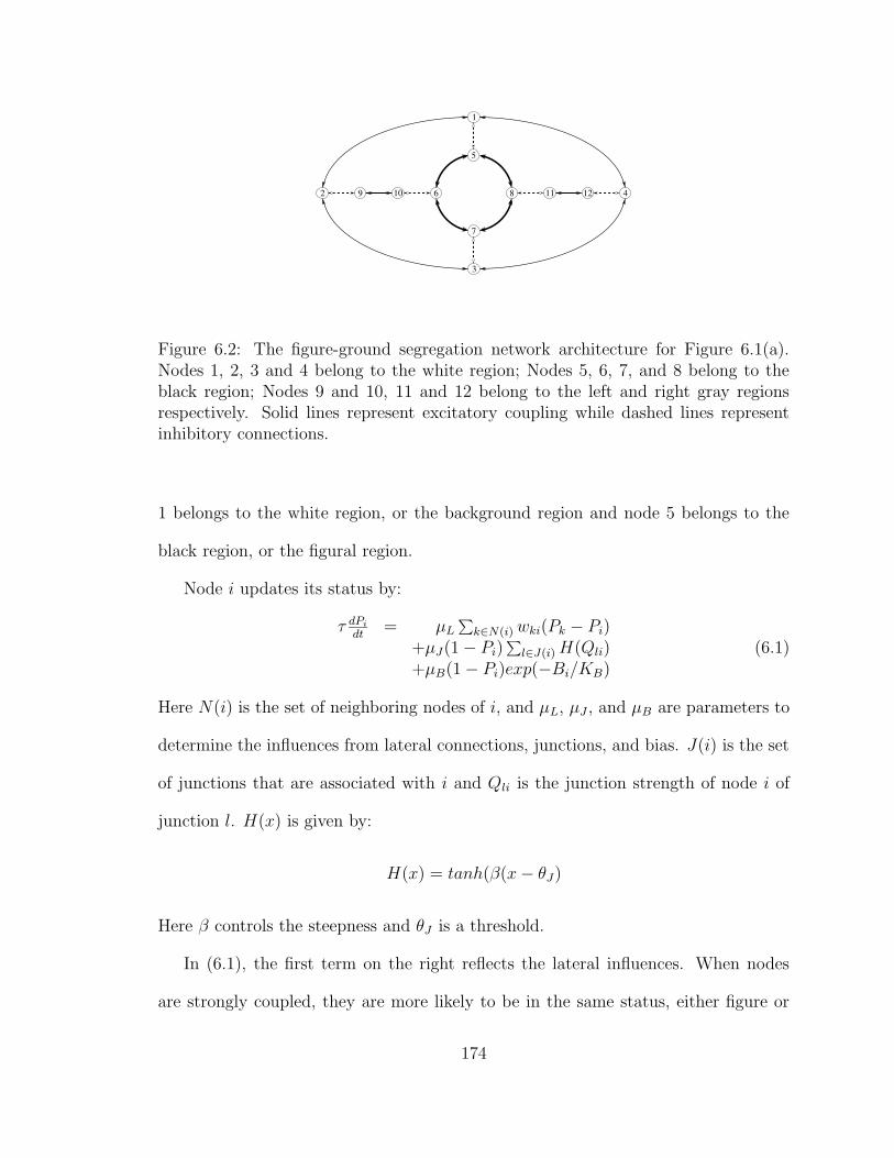
92 6
5
8
3
1
4
7
10 11 12
Figure 6.2: The figure-ground segregation network architecture for Figure 6.1(a).Nodes 1, 2, 3 and 4 belong to the white region; Nodes 5, 6, 7, and 8 belong to theblack region; Nodes 9 and 10, 11 and 12 belong to the left and right gray regionsrespectively. Solid lines represent excitatory coupling while dashed lines representinhibitory connections.
1 belongs to the white region, or the background region and node 5 belongs to the
black region, or the figural region.
Node i updates its status by:
τ dPi
dt= µL
∑
k∈N(i)wki(Pk − Pi)+µJ(1− Pi)
∑
l∈J(i)H(Qli)+µB(1− Pi)exp(−Bi/KB)
(6.1)
Here N(i) is the set of neighboring nodes of i, and µL, µJ , and µB are parameters to
determine the influences from lateral connections, junctions, and bias. J(i) is the set
of junctions that are associated with i and Qli is the junction strength of node i of
junction l. H(x) is given by:
H(x) = tanh(β(x− θJ)
Here β controls the steepness and θJ is a threshold.
In (6.1), the first term on the right reflects the lateral influences. When nodes
are strongly coupled, they are more likely to be in the same status, either figure or
174
background. Second term incorporates junction information. In other words, at a
T-junction, segments that are more smooth are more likely to be figural. The third
term is a bias term, where Bi is the bias introduced to simulate human perception.
After all the nodes are updates, the competition between paired nodes is through
normalization based on the assumption that only one of the paired nodes should be
figural at a given time. Suppose that j is the corresponding paired node of i, we have:
P(t+1)i = P t
i /(Pti + P t
j ) (6.2a)
P(t+1)j = P t
j /(Pti + P t
j ) (6.2b)
As a dynamic system, this shares some similarities with relaxation labeling tech-
niques [55]. Because the status of a node is only influenced by the nodes in a local
neighborhood in the network, as shown in Figure 6.2, the figure-ground segregation
network defines a Markov random field. This shares some similarities with the Markov
random fields proposed by Zhu [146] for perceptual organization. As will be demon-
strated later, our model can simulate many perceptual phenomena while the model
by Zhu [146] is a generic and theoretical model for shape modeling and perceptual
organization.
6.2.2 Incorporation of Gestalt Rules
Without introducing grouping cues such as T-junctions and preferences, the solu-
tion of the network is not well defined. To generate behavior that is consistent with
human perception, we incorporate grouping cues and some Gestalt grouping princi-
ples. As the network provides a generic model, many other rules can be incorporated
in a similar manner.
175
T-junctions T-junctions provide important cues for determining relative depth
[97] [141]. In Williams and Hanson’s model [141], T-junctions are imposed as topolog-
ical constraints. Given a T-junction l, the initial strength for node i that is associated
with l is:
Qli =exp(−α(i,c(i))/KT )
1/2∑
k∈NJ (l)exp(−α(k,c(k))/KT )
where KT is a parameter, NJ(l) is a set of all the nodes associated with junction l,
c(i) is the other node in NJ(l) that belongs to the same region as node i, and α(ij) is
the angle between segments i and j.
Non-accidentalness Non-accidentalness tries to capture the intrinsic relation-
ships among segments [86]. In our system, an additional connection is introduced to
node i if it is aligned well with a node j from the same region and j 6∈ N(i) initially.
The connection weight wij is a function of distance and angle between the involved
ending points. This can also be viewed as virtual junctions, resulting in virtual con-
tours and conversion of a corner into a T-junction if involving nodes become figural.
This corresponds to the organization criterion proposed by Geiger et al. [34].
Shape information Shape information plays a central role in Gestalt princi-
ples. For example, that virtual contours are vivid in Figure 6.8(a) but not in Figure
6.8(b) is due to the figural properties [64]. Shape information is incorporated through
enhancing lateral connections. In this chapter, we consider local symmetry. Let j
and k be the two neighboring nodes of i.
wij = 1 + C exp(−|αij − αki|/Kα)∗exp(−(Lj/Lk + Lk/Lj − 2)/KL))
(6.3)
176

Essentially (6.3) strengthens the lateral connections when the two neighboring seg-
ments of i are symmetric. Those nodes are then strongly grouped together according
to (6.1), resulting in different perceptions for Figure 6.8 (a) and (b).
Preferences Human perceptual systems often prefer some organizations over
the others. In this model, we incorporated a well-known figure-ground segregation
principle, called closedness. In other words, the system prefers regions over holes. In
current implementation, we set Bi = 1.0 if node i is part of a hole and otherwise
Bi = 0.
6.2.3 Temporal Properties of the Network
After we construct the figure-ground segregation network, there are two funda-
mental questions to be addressed. First we need to demonstrate that the equilibrium
state of the system gives a desired solution. Second, we need to show that the system
converges to the desired state. Here we demonstrate those using the example shown
in Figure 6.2. Figure 6.3 shows the temporal behavior of the network. First, the sys-
tem approaches to a stable solution. For figure-ground segregation, we can binarize
the status of each node using threshold 0.5. In this case, the system convergences
very quickly. In other words, the system outputs the solution in a few iterations.
Second, the system generates the correct perception. The black region is occluding
other regions while gray regions are occluding the white region. For example, P5 is
close to 1 and thus segment 5 is figural, and P1 is close to 0 and thus segment 1 is at
background.
177

1 5
2 6
3 7
4 8
9 11
10 12Time Time
Figure 6.3: Temporal behavior of each node in the network shown in Figure 6.2. Eachplot shows the status of the node with respect to the time. The dashed line is 0.5.
6.3 Surface Completion
After the figure-ground segregation is solved, surface completion and shape de-
composition can be implemented in a straightforward manner. Currently this stage is
implemented through diffusion. Because the ownership of each boundary segment is
known, fixed heat sources are generated along occluding boundaries, and the occlud-
ing boundaries naturally block diffusion. This method is similar to the one used by
Geiger et al. [34] for generating salient surfaces. However, in their approach, because
the hypotheses are defined only at junction points, fixed heat sources for diffusion
have to be given. On the other hand, in our model, fixed heat sources are generated
automatically along the occluding boundaries. In other words, the hypotheses in our
system are defined along boundaries, not at junction points.
178

To be more precise, regions from local segmentation are now grouped into diffusion
groups based on the average gray value and that if they are occluded by common
regions. Segments that belong to one diffusion group are diffused simultaneously. For
a figural segment, a buffer with a given radius is generated. Within the buffer, the
values are set to 1 for pixels belonging to the region and 0 otherwise. If there is no
figural segment in the diffusion group, it is the background, which is always the entire
image. Because the figure-ground segregation has been solved, with respect to the
diffusion group, only the parts that are being occluded need to be completed. Now
the problem becomes a well-defined mathematical problem. We need to solve the
heat equation with given boundary conditions. Currently, diffusion is implemented
though local diffusion. The results from diffusion are then binarized using threshold
0.5.
Figure 6.4 shows the results of Figure 6.1 after surface completion. Here the
two gray regions are grouped together through surface completion because occluded
boundaries allow diffusion. Figure 6.5(a) shows the result using a layered representa-
tion to show the relative depth between the surfaces. While the order in this example
is well defined, in general the system can handle surfaces that are overlapped with
each other, making the order ill-defined.
6.4 Experimental Results
For all the experiments shown in this chapter, we use a fixed set of parameters
for the figure-ground segregation network. Given an input image, the system auto-
matically constructs the network and establishes the connections based on the rules
discussed in Section 2.2.
179

(a) (b) (c)
Figure 6.4: Surface completion results for Figure 6.1(a). (a) White region. (b) Grayregion. (c) Black region.
Figure 6.5: Layered representation of surface completion for results shown in Figure6.4.
180
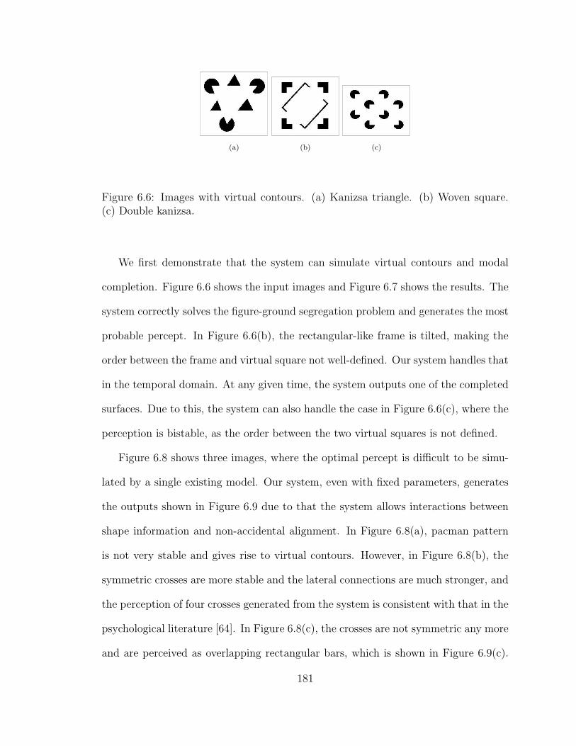
(a) (b) (c)
Figure 6.6: Images with virtual contours. (a) Kanizsa triangle. (b) Woven square.(c) Double kanizsa.
We first demonstrate that the system can simulate virtual contours and modal
completion. Figure 6.6 shows the input images and Figure 6.7 shows the results. The
system correctly solves the figure-ground segregation problem and generates the most
probable percept. In Figure 6.6(b), the rectangular-like frame is tilted, making the
order between the frame and virtual square not well-defined. Our system handles that
in the temporal domain. At any given time, the system outputs one of the completed
surfaces. Due to this, the system can also handle the case in Figure 6.6(c), where the
perception is bistable, as the order between the two virtual squares is not defined.
Figure 6.8 shows three images, where the optimal percept is difficult to be simu-
lated by a single existing model. Our system, even with fixed parameters, generates
the outputs shown in Figure 6.9 due to that the system allows interactions between
shape information and non-accidental alignment. In Figure 6.8(a), pacman pattern
is not very stable and gives rise to virtual contours. However, in Figure 6.8(b), the
symmetric crosses are more stable and the lateral connections are much stronger, and
the perception of four crosses generated from the system is consistent with that in the
psychological literature [64]. In Figure 6.8(c), the crosses are not symmetric any more
and are perceived as overlapping rectangular bars, which is shown in Figure 6.9(c).
181

(a) (b) (c)
Figure 6.7: Surface completion results for the corresponding image in Figure 6.6.
Both models by Williams and Hanson [141] and Geiger et al. [34] do not correctly
handle the case shown in Figure 6.8(b).
Figure 6.10 shows three variations of pacman images. The results from our system
are shown in Figure fig:pacman-statck. While our system can correctly handle all of
them in a similar way and generate correct results, edge-based approaches tend to have
problems, as pointed out in [141]. This is because the edges have different contrast
signs. Theses examples are strong evidence for boundary-pair representation.
Figure 6.12 (a) and (b) show well-known examples by Bregman [9]. While the
edge elements in both cases are similar, the perception is quite different. In Figure
6.12(a), there is no perceptual grouping and parts of B’s remain fragmented. However,
when occlusion is introduced as in Figure 6.12(b), perceptual grouping is evident and
fragments of B’s are grouped together. These perceptions are consistent with our
182
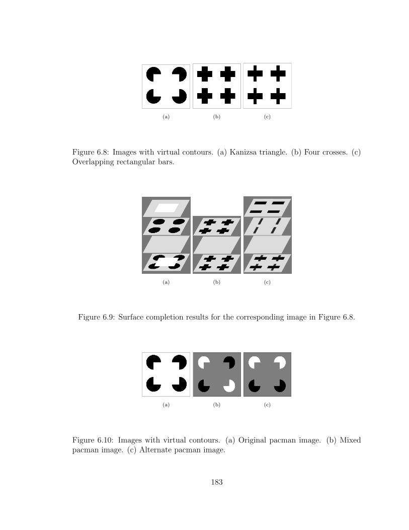
(a) (b) (c)
Figure 6.8: Images with virtual contours. (a) Kanizsa triangle. (b) Four crosses. (c)Overlapping rectangular bars.
(a) (b) (c)
Figure 6.9: Surface completion results for the corresponding image in Figure 6.8.
(a) (b) (c)
Figure 6.10: Images with virtual contours. (a) Original pacman image. (b) Mixedpacman image. (c) Alternate pacman image.
183
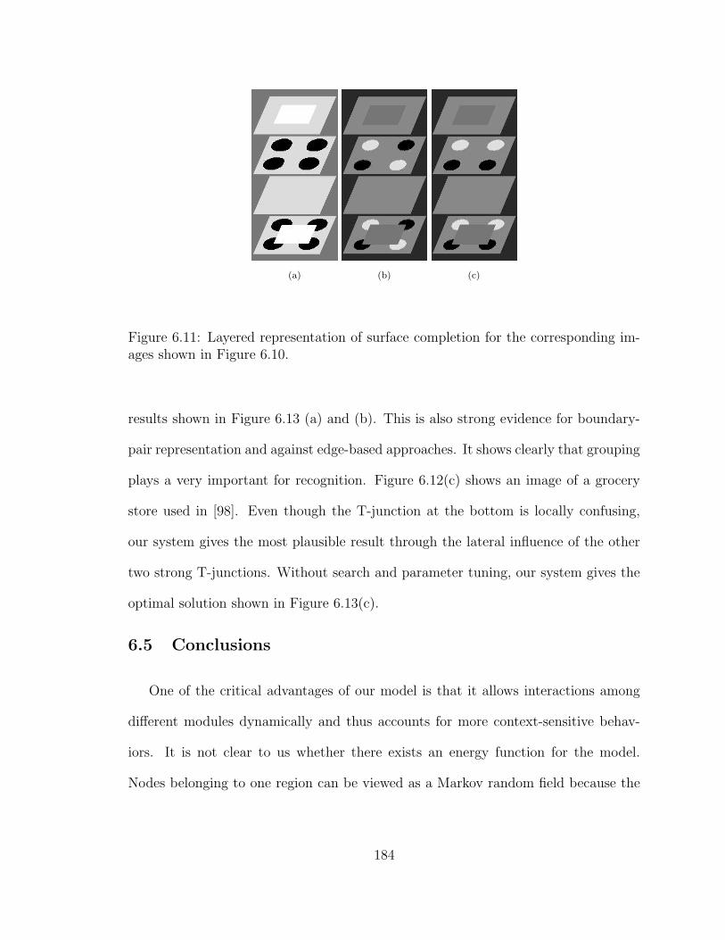
(a) (b) (c)
Figure 6.11: Layered representation of surface completion for the corresponding im-ages shown in Figure 6.10.
results shown in Figure 6.13 (a) and (b). This is also strong evidence for boundary-
pair representation and against edge-based approaches. It shows clearly that grouping
plays a very important for recognition. Figure 6.12(c) shows an image of a grocery
store used in [98]. Even though the T-junction at the bottom is locally confusing,
our system gives the most plausible result through the lateral influence of the other
two strong T-junctions. Without search and parameter tuning, our system gives the
optimal solution shown in Figure 6.13(c).
6.5 Conclusions
One of the critical advantages of our model is that it allows interactions among
different modules dynamically and thus accounts for more context-sensitive behav-
iors. It is not clear to us whether there exists an energy function for the model.
Nodes belonging to one region can be viewed as a Markov random field because the
184

(a) (b) (c)
Figure 6.12: Bregman and real images. (a) and (b) Examples by Bregman [9]. (c) Agrocery store image.
(a) (b) (c)
Figure 6.13: Surface completion results for images shown in Figure 6.12.
185

(a) (b) (c)
Figure 6.14: Bistable perception. (a) Face-vase input image. (b) Faces as figures. (c)Vase as figure.
influence is defined locally in the network. However, the inhibition between paired
nodes introduced in (6.2) complicates the system analysis.
Multiple solutions can also be generated by our models. A simple way is through
self-inhibition. Here we demonstrate that through habituation [132]. It is well known
that the strength of responses decreases when a stimulus is presented repeatedly.
Figure 6.14(a) shows an image, where either two faces or vase can be perceived, but
not both at the same time. Figure 6.14(b) and (c) show the two possible results
using layered representation. In Figure 6.14(b), two faces are perceived and and the
vase is suppressed into the background; Figure 6.14(c) shows the other case. Here
the differences can be seen from the middle layer. By introducing habituation, our
system offers a computational explanation. As shown in Figure 6.15, two faces and
vase alternate to be figural, resulting in bistable percept. This example demonstrates
that top-down influence from memory and recognition can be naturally incorporated
in the network.
186
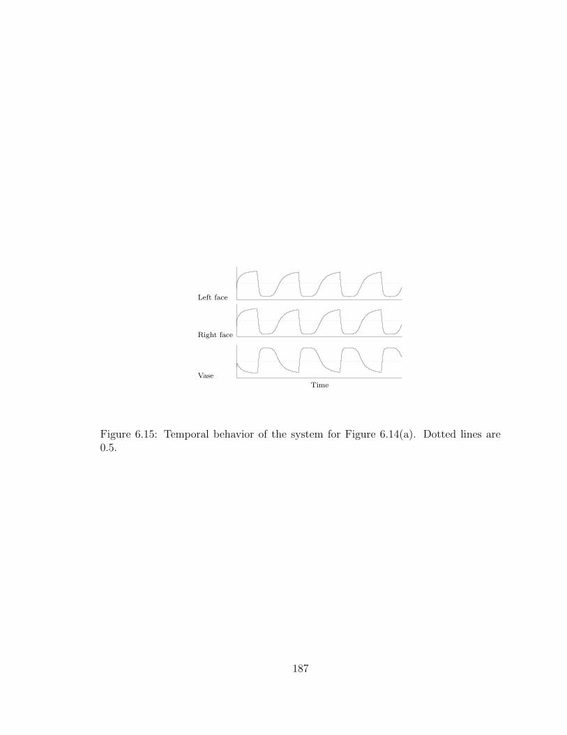
Left face
Right face
Vase
Time
Figure 6.15: Temporal behavior of the system for Figure 6.14(a). Dotted lines are0.5.
187
CHAPTER 7
EXTRACTION OF HYDROGRAPHIC REGIONS FROM
REMOTE SENSING IMAGES USING AN OSCILLATOR
NETWORK WITH WEIGHT ADAPTATION
We study the extraction of objects with accurate boundaries from remote sensing
images. We use a locally excitatory globally inhibitory oscillator network (LEGION)
as a representational framework to combine the advantages of classification-based
methods and locally coupled networks. A multi-layer perceptron is used to select
seed points within regions to be extracted. The boundaries of the extracted regions
are accurately located through a topology preserving LEGION network. A novel
weight-adaptation method, which preserves significant boundaries between regions
and smoothes details due to variations and noise, is employed to increase the robust-
ness of the system. Together, these provide a generic framework for feature extraction.
A functional system has been developed and applied to hydrographic region extrac-
tion from Digital Orthophoto Quarter-Quadrangle (DOQQ) images. Experimental
results show that the extracted regions are comparable with existing topographic
maps and can be used for map revision. Preliminary versions appear in [78] [85] [84]
[76] [77]. Weight adaptation is first proposed by Chen et al [17].
188
7.1 Introduction
With the availability of remotely sensed high-resolution imagery and advances
in computing technologies, cost-effective and efficient ways to generate accurate ge-
ographic information are possible. Because geographic information is implicitly en-
coded in images, the critical step is how to extract geographic information from im-
ages and make it explicit. While humans can efficiently and robustly extract desired
features from images, image understanding is regarded as one of the most difficult
problems in machine intelligence. For remote sensing applications, classification is
one of the most commonly used techniques to extract quantitative information from
images. Because multilayer perceptrons can potentially approximate complex deci-
sion functions, they have been widely used for solving many practical problems and
specifically in remote sensing applications [38] [126] [2] [121]. The major advantages
of neural network approaches are that no prior information is required and parameters
can be obtained automatically through training [115]. A major disadvantage is that
neural networks classify each pixel individually and do not incorporate contextual
information, i.e., the relationship among neighboring pixels, resulting in relatively
poor performance when the variations within a class are large. To illustrate the prob-
lem, Figure 7.1(a) shows a noisy synthetic image and Figure 7.1(b) shows the ground
truth image. A three-layer perceptron is trained using a standard back-propagation
algorithm [46] with 12 positive and 12 negative examples as shown in Figure 7.1(c).
Figure 7.1(d) shows the classification result. While the central regions are classified
correctly, the boundaries are not located accurately, resulting in a large classification
error as shown in Table 7.1.
189
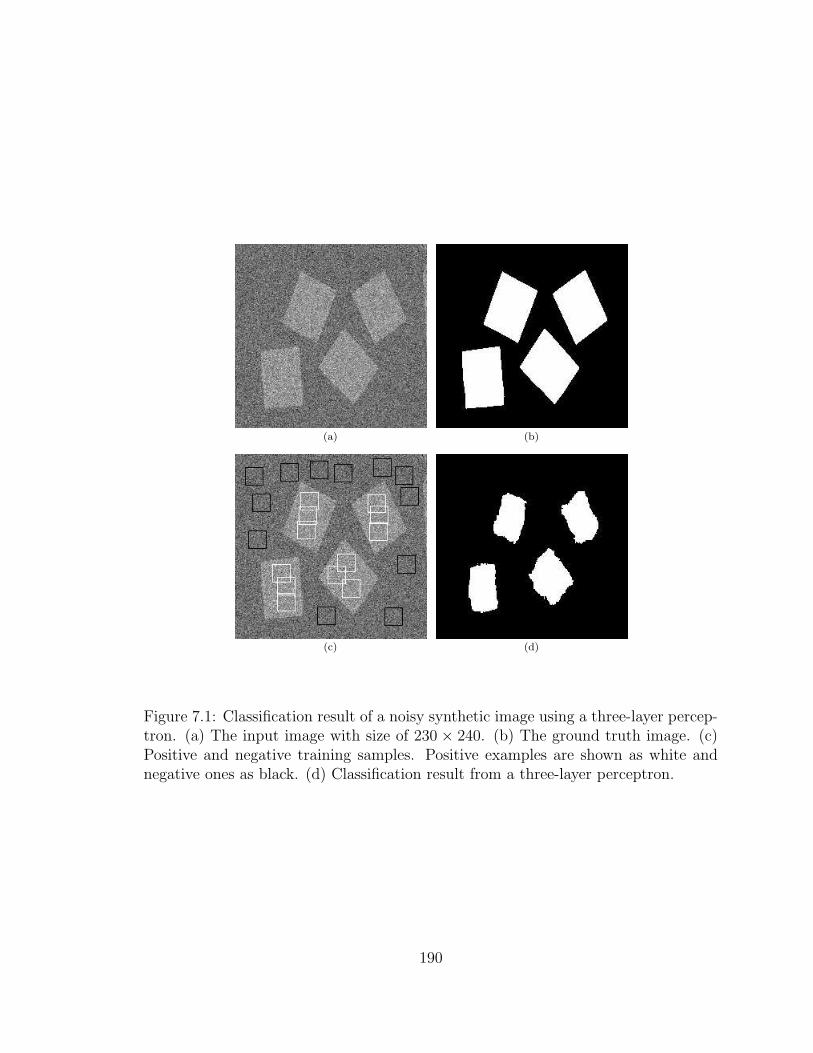
(a) (b)
(c) (d)
Figure 7.1: Classification result of a noisy synthetic image using a three-layer percep-tron. (a) The input image with size of 230 × 240. (b) The ground truth image. (c)Positive and negative training samples. Positive examples are shown as white andnegative ones as black. (d) Classification result from a three-layer perceptron.
190

Classification can be posed as a statistical mapping from observations to specified
classes. In general, the design of a statistical pattern classification algorithm requires
some prior statistical information. With assumptions of specific distribution and er-
ror functions, many statistical classifiers have been proposed [25] [109] and have been
widely used in remote sensing applications [3] [109] [39]. The statistical formulation
provides a unified way to incorporate prior knowledge and contextual information.
Contextual classifiers explicitly incorporate contextual information in classification
[32] [57], resulting in significant performance improvement. Markov Random Fields,
as a special case in specifying contextual information, have been successful in image
restoration, modeling, and segmentation [35]. Essentially by specifying joint distri-
butions through Gibbs’ distribution, the central computation task is an optimization
problem for non-convex energy functions with high dimensionality. Because ideal
optimization is computationally prohibitive, in practice only a local optimum can
be obtained. With approximate but more efficient optimization algorithms, Markov
Random Fields have been applied widely in remote sensing applications [110] [118].
As we can see from the development of classification algorithms, one of the criti-
cal issues in improving classification performance is how to incorporate contextual
information.
We attempt to develop a framework for automated feature extraction that can
derive accurate geographic information for map revision and be applied to very large
images, such as DOQQ images. In this chapter, we pose the automated feature ex-
traction problem as a binding problem. Pixels that belong to desired regions should
be bound together to form desired objects. We use a LEGION network [123] [134]
[135], which is a generic framework for binding and image segmentation. As shown
191
analytically, LEGION networks can achieve both synchronization within an oscillator
group representing a region and desynchronization among different oscillator groups
rapidly. This offers a theoretical advantage over pure local networks such as Markov
Random Fields [35], where efficient convergence has not been established in general.
To improve the performance, we incorporate contextual information through a weight
adaptation method proposed by Chen et al [17]. As multiple scales in edge detection
algorithms [74] can be viewed as a way of incorporating contextual information by
relating detected structures at different scales, weight adaptation can be viewed as a
concrete multiple scale approach with two scales. Instead of applying the same opera-
tors at different scales, in weight adaptation, statistical information from a larger scale
is derived and mainly used to govern a locally coupled adaptation process, resulting in
accurate boundary localization and robustness to noise. We assume that features to
be extracted are specified through examples and use a multilayer perceptron trained
through back-propagation [46] for seed selection. To reduce the number of necessary
training samples and increase the generalization of the classification method, instead
of classifying the entire image, we use a multilayer perceptron to identify seed points
only. LEGION is then used to provide a framework for integration. We have de-
veloped a functioning system using the proposed method for hydrographic feature
extraction from DOQQ images and have obtained satisfactory results.
This chapter is organized as follows. Section 7.2 introduces weight adaptation.
Section 7.3 describes a multilayer perceptron for automated seed selection. Section
7.4 provides experimental results using DOQQ images. Section 7.5 concludes the
chapter with further discussions.
192

7.2 Weight Adaptation
Given LEGION dynamics, as presented in Section 2.2, to extract desired features,
we need to form local connections based on the input image. To facilitate the following
notations for weight adaptation, we re-write the coupling term Sij in (2.1a) as [17]:
Sij =
∑
(k,l)∈N(i,j)H(xkl)/(1 + |Wij;kl|)log
(
∑
(k,l)∈N(i,j)H(xkl) + 1) −WzH(z − θz), (7.1)
As in (2.2), the first term here is the total excitatory coupling that oscillator (i, j)
receives from the oscillators in a local neighborhood N(i, j), and Wij;kl is the dynamic
connection from oscillator (k, l) to (i, j). Here Wij;kl encodes dissimilarity to simplify
the equations for weight adaptation, hence the reciprocal3. Note that, unlike in (2.2),
the first term implements a logarithmic grouping rule [17], which generates better
segmentation results in general.
As illustrated in Figure 2.3, effective couplings in a local neighborhood are used.
Without introducing assumptions about the desired features, Wij;kl in general can
be formed based on the intensity values at the corresponding pixels (i, j) and (k, l)
in the input image. However, due to variations and noise in real images, individual
pixel values are not reliable, and the resulting connections would be noisy and give
undesirable results. Figure 7.2(a) shows a one-dimensional signal which is a row from
the image shown in Figure 7.1(a). As shown in Figure 7.2(b), the connections formed
based on input intensity values are noisy, which lead to undesired region boundaries.
3This interpretation is different from a previous one used in (2.2) [123] [135]. After algebraicmanipulations, the equations can be re-written in terms of the previous, more conventional inter-pretation.
193

(a)
(b)
(c)
(d)
Figure 7.2: Lateral connection evolution through weight adaptation illustrated usingthe 170th row from the image shown in Figure 7.1(a). (a) The original signal. (b) Ini-tial connection weights. (c) Connection weights after 40 iterations. (d) Correspondingsmoothed signal.
194

To overcome this problem, we use a weight adaptation method for noise removal
and feature preservation [17]. For each oscillator in the network, two kinds of con-
nections, namely, fixed and dynamic connections, are introduced. For oscillator (i, j),
the fixed connectivity specifies a group of neighboring oscillators which affect the os-
cillator, and the associated neighborhood is called lateral neighborhood Nl(i, j). On
the other hand, the dynamic connectivity encodes the transient relationship between
two oscillators in a local neighborhood during weight adaption, and the associated
neighborhood is called local neighborhood N(i, j). To achieve accurate boundary
localization, in this chapter, N(i, j) is defined as the eight nearest neighborhood of
(i, j), as depicted in Figure 2.3. Fixed connection weights are established based on the
input image, while dynamic connection weights adapt themselves for noise removal
and feature preservation, resulting interactions between two scales. Intuitively, dy-
namic weights between two oscillators should be adapted so that the absolute dynamic
weight becomes small if the corresponding pixels are in a homogeneous region, while
the weight should remain relatively large if the corresponding pixels cross a boundary
between different homogeneous regions. Based on the observation that most of the
discontinuities in the lateral neighborhood Nl(i, j) correspond to significant features,
such discontinuities should remain unchanged and be used to control the speed of
weight adaptation for preserving features. Such discontinuities in the lateral neigh-
borhood are called lateral discontinuities [17]. Furthermore, because proximity is a
major grouping principle [111], we use another measure that reflects local discontinu-
ities sensitive to the changes of local attributes among local oscillators. The lateral
neighborhood provides a more reliable statistical context, by which the weight adap-
tation algorithm is governed. The local neighborhood utilizes the statistical context
195

and local geometrical constraints to adaptively change the local connections. These
two discontinuity measures are jointly incorporated in weight adaptation.
Mathematically, the weight adaption method is formulated as follows. For oscil-
lator (i, j), the weight of its fixed connection from oscillator (k, l) in Nl(i, j), Tij;kl, is
defined as the difference between the external stimuli received by (i, j) and (k, l), i.e.
Tij;kl = Ikl − Iij. (7.2)
Here Iij and Ikl are the intensities of pixels (i, j) and (k, l) respectively. For oscillator
(i, j), the fixed connections exist only in Nl(i, j) and Tij;kl = −Tkl;ij. On the other
hand, to achieve accurate boundary localization, a dynamic connection weight from
oscillator (k, l) to oscillator (i, j), Wij;kl, is defined only within a local neighborhood
N(i, j) and initialized to the corresponding fixed weight, i.e., W(0)ij;kl = Tij;kl. Dynamic
weight |W (t)ij;kl| encodes the dissimilarity between oscillators (i, j) and (k, l) at time t.
First, the variance of all the fixed weights associated with an oscillator is used to
measure its lateral discontinuities. For oscillator (i, j), the mean of its fixed weights
on Nl(i, j), µij, is calculated using
µij =
∑
(k,l)∈Nl(i,j) Tij;kl
|Nl(i, j)|. (7.3)
Accordingly, we compute the variance of its fixed weights, σ2ij, by
σ2ij =
∑
(k,l)∈Nl(i,j)
(
Tij;kl − µij
)2
|Nl(i, j)|
=
∑
(k,l)∈Nl(i,j) T2ij;kl
|Nl(i, j)|−(
∑
(k,l)∈Nl(i,j) Tij;kl
|Nl(i, j)|
)2
. (7.4)
The variance, σ2ij, is normalized through
σ2ij =
σ2ij − σ2
min
σ2max − σ2
min
. (7.5)
196
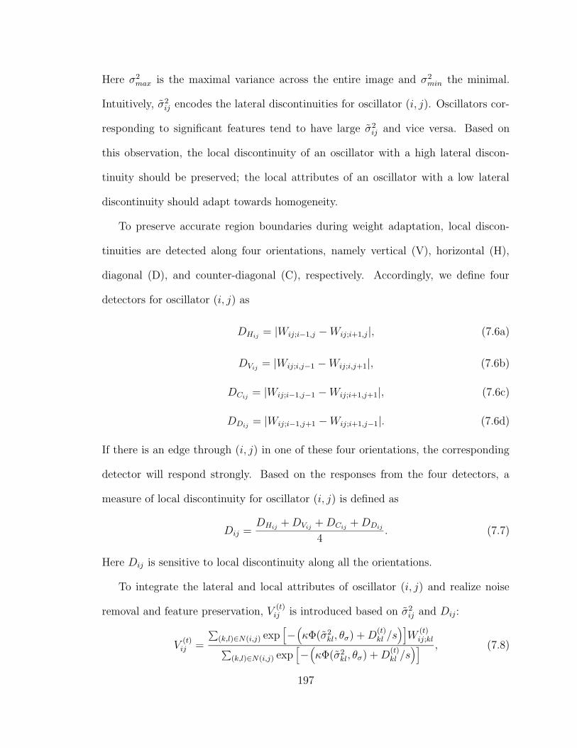
Here σ2max is the maximal variance across the entire image and σ2
min the minimal.
Intuitively, σ2ij encodes the lateral discontinuities for oscillator (i, j). Oscillators cor-
responding to significant features tend to have large σ2ij and vice versa. Based on
this observation, the local discontinuity of an oscillator with a high lateral discon-
tinuity should be preserved; the local attributes of an oscillator with a low lateral
discontinuity should adapt towards homogeneity.
To preserve accurate region boundaries during weight adaptation, local discon-
tinuities are detected along four orientations, namely vertical (V), horizontal (H),
diagonal (D), and counter-diagonal (C), respectively. Accordingly, we define four
detectors for oscillator (i, j) as
DHij= |Wij;i−1,j −Wij;i+1,j |, (7.6a)
DVij= |Wij;i,j−1 −Wij;i,j+1|, (7.6b)
DCij= |Wij;i−1,j−1 −Wij;i+1,j+1|, (7.6c)
DDij= |Wij;i−1,j+1 −Wij;i+1,j−1|. (7.6d)
If there is an edge through (i, j) in one of these four orientations, the corresponding
detector will respond strongly. Based on the responses from the four detectors, a
measure of local discontinuity for oscillator (i, j) is defined as
Dij =DHij
+DVij+DCij
+DDij
4. (7.7)
Here Dij is sensitive to local discontinuity along all the orientations.
To integrate the lateral and local attributes of oscillator (i, j) and realize noise
removal and feature preservation, V(t)ij is introduced based on σ2
ij and Dij:
V(t)ij =
∑
(k,l)∈N(i,j) exp[
−(
κΦ(σ2kl, θσ) +D
(t)kl /s
)]
W(t)ij;kl
∑
(k,l)∈N(i,j) exp[
−(
κΦ(σ2kl, θσ) +D
(t)kl /s
)] , (7.8)
197

where s (s > 0) is a parameter that determines to what extent local discontinuities
should be preserved, and κ (κ > 0) is to control to what extent features should be
preserved in terms of lateral discontinuities during weight adaptation. The function
Φ(ν, θ) is a rectification function, defined as Φ(ν, θ) = ν if ν ≥ θ and Φ(ν, θ) = 0 oth-
erwise. To deal with variations due to noisy details, θσ (0 ≤ θσ ≤ 1) is introduced to
alleviate the influence of noise in the estimation of lateral discontinuities. The degree
of lateral discontinuities in an image gives a measure of the significance of the corre-
sponding discontinuities. In (7.8), if the lateral discontinuities of all the oscillators in
N(i, j) are similar, their local discontinuities should play a dominant role in updat-
ing V(t)ij . In this case, the contribution of dynamic weight W
(t)ij;kl in updating V
(t)ij is
determined by the corresponding local discontinuity D(t)kl of oscillator (k, l) in N(i, j).
If D(t)kl is small, W
(t)ij;kl has a large contribution, and vice versa. The local attributes of
oscillator (i, j) are changed through updating V(t)ij so that the dissimilarity between
(i, j) and its neighboring oscillators is reduced with respect to s. Noise removal along
with feature preservation is achieved through the reduction of dissimilarity in terms
of local discontinuities. On the other hand, when neighboring oscillators of (i, j)
have different lateral discontinuities, both lateral and local discontinuities must be
employed in determining the contribution from W(t)ij;kl to V
(t)ij . In this case, when
the overall discontinuities associated with oscillator (k, l) are relatively small, W(t)ij;kl
makes a large contribution. Lateral and local discontinuities jointly provide a robust
way to realize feature preservation and noise removal for those oscillators associated
with large lateral discontinuities, i.e. σ2kl ≥ θσ. The local attributes of oscillator (i, j)
are adapted towards reduction of the dissimilarity between (i, j) and the neighbor-
ing oscillators with relatively small overall discontinuities. The dissimilarity between
198
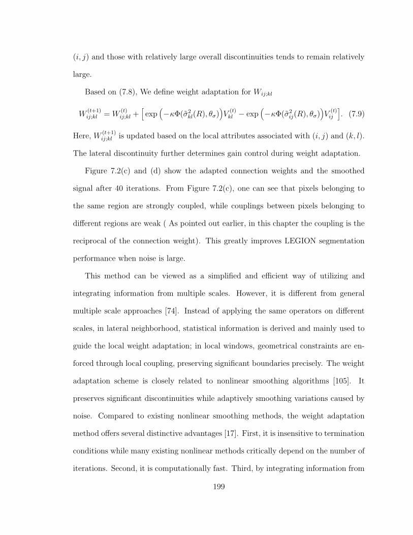
(i, j) and those with relatively large overall discontinuities tends to remain relatively
large.
Based on (7.8), We define weight adaptation for Wij;kl
W(t+1)ij;kl = W
(t)ij;kl +
[
exp(
−κΦ(σ2kl(R), θσ)
)
V(t)kl − exp
(
−κΦ(σ2ij(R), θσ)
)
V(t)ij
]
. (7.9)
Here, W(t+1)ij;kl is updated based on the local attributes associated with (i, j) and (k, l).
The lateral discontinuity further determines gain control during weight adaptation.
Figure 7.2(c) and (d) show the adapted connection weights and the smoothed
signal after 40 iterations. From Figure 7.2(c), one can see that pixels belonging to
the same region are strongly coupled, while couplings between pixels belonging to
different regions are weak ( As pointed out earlier, in this chapter the coupling is the
reciprocal of the connection weight). This greatly improves LEGION segmentation
performance when noise is large.
This method can be viewed as a simplified and efficient way of utilizing and
integrating information from multiple scales. However, it is different from general
multiple scale approaches [74]. Instead of applying the same operators on different
scales, in lateral neighborhood, statistical information is derived and mainly used to
guide the local weight adaptation; in local windows, geometrical constraints are en-
forced through local coupling, preserving significant boundaries precisely. The weight
adaptation scheme is closely related to nonlinear smoothing algorithms [105]. It
preserves significant discontinuities while adaptively smoothing variations caused by
noise. Compared to existing nonlinear smoothing methods, the weight adaptation
method offers several distinctive advantages [17]. First, it is insensitive to termination
conditions while many existing nonlinear methods critically depend on the number of
iterations. Second, it is computationally fast. Third, by integrating information from
199

different scales, this method can generate better results. Quantitative comparisons
with other methods, including various smoothing algorithms, are provided in [17].
7.3 Automated Seed Selection
Both LEGION networks and weight adaptation methods are generic approaches,
where no assumptions about the features being extracted are made. To extract de-
sired features from remote sensing images, we need to specify relevant features. One
way to do this is to use certain parametric forms based on assumptions about the
statistical properties of features and noise. However, for map revision and other re-
mote sensing applications, images may be acquired under different conditions and
even through different sources, such as DOQQ images. These make it very difficult
to model the features using parametric forms. A more feasible way is to specify the
desired features through positive and negative examples. There are essentially two
broad categories of approaches for solving the problem. Statistical based approaches
need knowledge of statistical distribution [3] [115], which may not be available or
may be difficult to obtain due to different data sources and acquisition conditions.
Artificial neural networks provide an alternate approach. Because they can approxi-
mate arbitrary complex functions, artificial neural networks are suitable for describing
features being extracted in remote sensing applications, where many factors are in-
volved in generating the features in input images. The major advantages of using
neural networks include that no prior knowledge of statistical distribution is needed
and parameters can be obtained automatically through training [3] [115]. Artificial
neural networks, especially multilayer perceptrons, have been widely used in remote
sensing applications [38] [126] [2] [121].
200

To apply a multilayer perceptron, a number of design choices must be made.
These choices may greatly affect the convergence of the network and learning results.
For our task, we use a three-layer perceptron, with four input units, three hidden
units, and one output unit, as shown in Figure 7.3. It is trained using a standard
back-propagation algorithm [46]. If we present the pixels in the training examples
directly to the network, we observe that many training examples are necessary to
achieve good results. Due to the potential conflicting conditions, the network often
does not converge. To achieve rotational invariance and reduce the necessary number
of training samples, instead of presenting the training windows directly to the network
we extract several local attributes from training windows as input to the network.
More specifically, we use the average value, minimum value, maximum value, and
variance from training samples. These values are normalized to improve training and
classification results.
To further reduce the number of necessary training samples and deal with varia-
tions within features being extracted, we use a three-layer perceptron for seed selection
only. In other words, instead of classifying all the pixels directly, we train the network
to find pixels that are within a large region to be extracted. The accurate boundaries
are derived using an oscillator network with weight adaptation. As demonstrated
in the next section, a small of training samples are sufficient for very large images
with significant variations. Our training methodology offers a distinctive advantage
in reducing necessary training examples. In contrast, many experiments often divide
the entire data into training and test sets with approximately the same size to achieve
good performance [118], ending up using many more training samples.
201
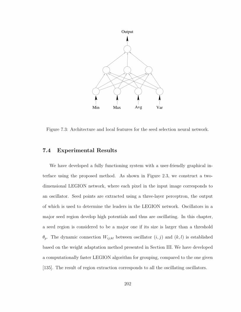
Min Max Avg Var
Output
Figure 7.3: Architecture and local features for the seed selection neural network.
7.4 Experimental Results
We have developed a fully functioning system with a user-friendly graphical in-
terface using the proposed method. As shown in Figure 2.3, we construct a two-
dimensional LEGION network, where each pixel in the input image corresponds to
an oscillator. Seed points are extracted using a three-layer perceptron, the output
of which is used to determine the leaders in the LEGION network. Oscillators in a
major seed region develop high potentials and thus are oscillating. In this chapter,
a seed region is considered to be a major one if its size is larger than a threshold
θp. The dynamic connection Wij;kl between oscillator (i, j) and (k, l) is established
based on the weight adaptation method presented in Section III. We have developed
a computationally faster LEGION algorithm for grouping, compared to the one given
[135]. The result of region extraction corresponds to all the oscillating oscillators.
202
7.4.1 Parameter Selection
Our method consists of three relatively independent systems. For LEGION net-
works, except Wz and θp, all other parameters are system parameters and application
independent. For weight adaptation, three parameters are involved. In order to
achieve optimal results, these parameters are application dependent and subject to
tuning. However, as demonstrated in [17], these parameters can be fixed for images
of a similar type. In this chapter, they are fixed for all the experiments: s = 10.0,
κ = 60.0, and θσ = 0.02. The lateral neighborhood Nl(i, j) consists of 7×7 oscillators.
Wij;kl is updated for 40 iterations using (7.9).
The three-layer perceptron for seed selection is trained using a standard back-
propagation with momentum. The learning rate is set to 0.025 and the momentum
parameter is set to 0.9. The activation function used is a sigmoid function, the
steepness parameter of which is 0.5. The training is terminated when the error from
all the samples is less than 0.05.
7.4.2 Synthetic Image
To demonstrate the capability of the proposed method, we have applied the sys-
tem to a noisy synthetic image shown in Figure 7.1(a). A three-layer perceptron is
trained using 12 positive and 12 negative samples, as shown in Figure 7.1(c). Each
sample is a window with 23× 23 pixels from the original image. Local attributes are
first calculated from the training samples and then fed to a three-layer perceptron as
input vectors. The classification result is shown in Figure 7.1(d). While the region
boundaries are not localized precisely, seed points within central regions are found
203
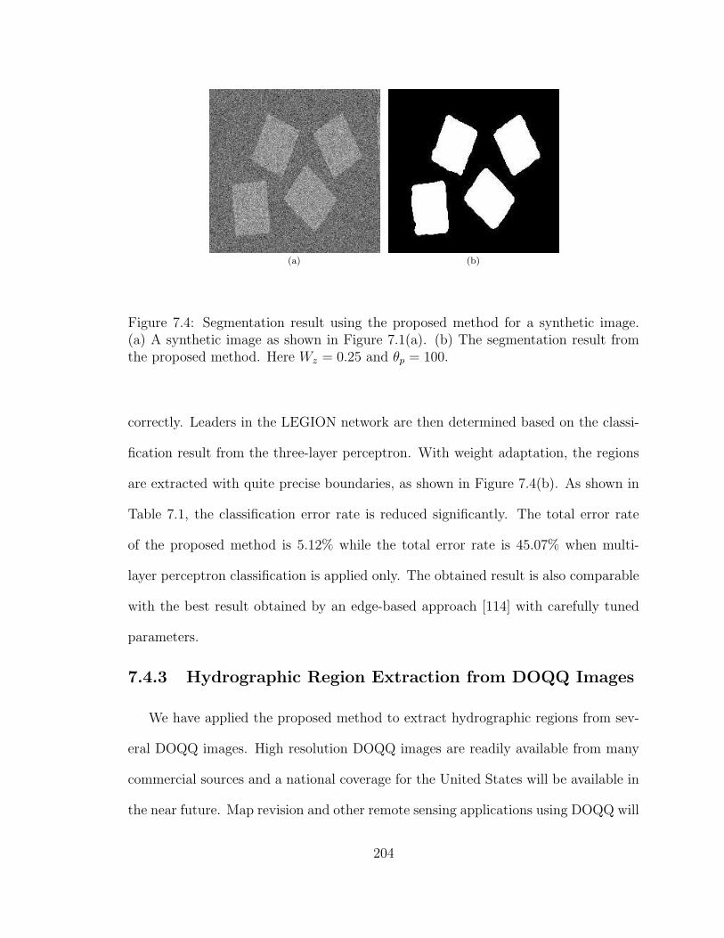
(a) (b)
Figure 7.4: Segmentation result using the proposed method for a synthetic image.(a) A synthetic image as shown in Figure 7.1(a). (b) The segmentation result fromthe proposed method. Here Wz = 0.25 and θp = 100.
correctly. Leaders in the LEGION network are then determined based on the classi-
fication result from the three-layer perceptron. With weight adaptation, the regions
are extracted with quite precise boundaries, as shown in Figure 7.4(b). As shown in
Table 7.1, the classification error rate is reduced significantly. The total error rate
of the proposed method is 5.12% while the total error rate is 45.07% when multi-
layer perceptron classification is applied only. The obtained result is also comparable
with the best result obtained by an edge-based approach [114] with carefully tuned
parameters.
7.4.3 Hydrographic Region Extraction from DOQQ Images
We have applied the proposed method to extract hydrographic regions from sev-
eral DOQQ images. High resolution DOQQ images are readily available from many
commercial sources and a national coverage for the United States will be available in
the near future. Map revision and other remote sensing applications using DOQQ will
204
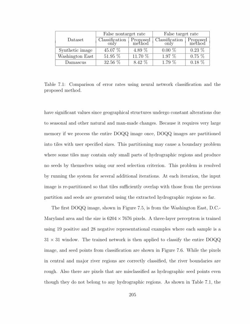
False nontarget rate False target rateDataset Classification Proposed Classification Proposed
only method only method
Synthetic image 45.07 % 4.89 % 0.00 % 0.23 %Washington East 51.95 % 11.70 % 1.97 % 0.75 %
Damascus 32.56 % 8.42 % 1.79 % 0.18 %
Table 7.1: Comparison of error rates using neural network classification and theproposed method.
have significant values since geographical structures undergo constant alterations due
to seasonal and other natural and man-made changes. Because it requires very large
memory if we process the entire DOQQ image once, DOQQ images are partitioned
into tiles with user specified sizes. This partitioning may cause a boundary problem
where some tiles may contain only small parts of hydrographic regions and produce
no seeds by themselves using our seed selection criterion. This problem is resolved
by running the system for several additional iterations. At each iteration, the input
image is re-partitioned so that tiles sufficiently overlap with those from the previous
partition and seeds are generated using the extracted hydrographic regions so far.
The first DOQQ image, shown in Figure 7.5, is from the Washington East, D.C.-
Maryland area and the size is 6204× 7676 pixels. A three-layer perceptron is trained
using 19 positive and 28 negative representational examples where each sample is a
31 × 31 window. The trained network is then applied to classify the entire DOQQ
image, and seed points from classification are shown in Figure 7.6. While the pixels
in central and major river regions are correctly classified, the river boundaries are
rough. Also there are pixels that are misclassified as hydrographic seed points even
though they do not belong to any hydrographic regions. As shown in Table 7.1, the
205

false target rate is 1.97%. Here the false target rate is the ratio of the number of non-
hydrographic pixels which are misclassified to the total number of true hydrographic
pixels. Similarly, the false nontarget rate is the ratio of the number of hydrographic
pixels that are misclassified to the total number of true hydrographic pixels. The
ground truth, as shown in Figure 7.8 is generated by manual seed selection based
on a 1:24,000 topographic map from the United States Geological Survey (see Figure
7.10(c) for example) and DOQQ image. Figure 7.9(b) is generated from Figure 7.9(a)
using the same procedure. Leaders in LEGION are determined with θp = 4000.
Because noisy seed points cannot develop high potentials, no hydrographic regions are
extracted around those pixels. We apply a LEGION network with weight adaptation
where there are leaders in the tile being processed. Figure 7.7 shows the result
from our system. As shown in Table 7.1, both the false target and false nontarget
rates are reduced dramatically. The false target rate is reduced to 0.75%. Also the
hydrographic region boundaries are localized much more accurately, and thus the
false nontarget rate is reduced. Mainly because the Kenil Worth Aquatic Gardens,
magnified in Figure 7.9(a), is not extracted, the false nontarget rate of the proposed
method still stands at 11.70%. Because the aquatic area is statistically very similar
to soil land, it is not possible to classify it correctly solely using the perceptron.
If we assume that seed points are correctly detected in the area, the proposed
method can correctly extract the aquatic region with high accuracy. The result,
shown in Figure 7.9(b), is generated by manually selecting seed points in the area.
This would reduce the error rate of the proposed method even further.
More importantly, major hydrographic regions are extracted with accurate bound-
aries and cartographic features, such as bridges and islands, are preserved well. These
206
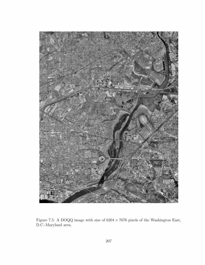
Figure 7.5: A DOQQ image with size of 6204× 7676 pixels of the Washington East,D.C.-Maryland area.
207

Figure 7.6: Seed pixels obtained by applying a trained three-layer perceptron to theDOQQ image shown in Figure 7.5. Seed pixels are marked as white and superimposedon the original image. The network is trained using 19 positive and 28 negativesamples, where each sample is a 31× 31 window.
208
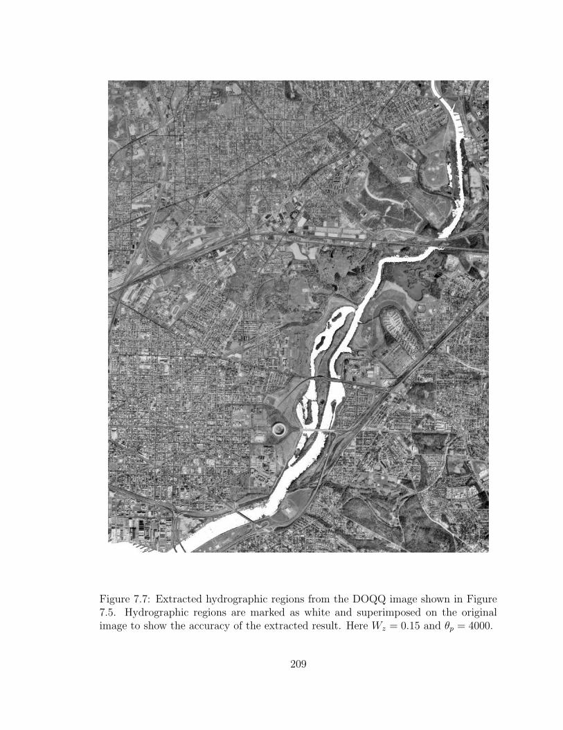
Figure 7.7: Extracted hydrographic regions from the DOQQ image shown in Figure7.5. Hydrographic regions are marked as white and superimposed on the originalimage to show the accuracy of the extracted result. Here Wz = 0.15 and θp = 4000.
209
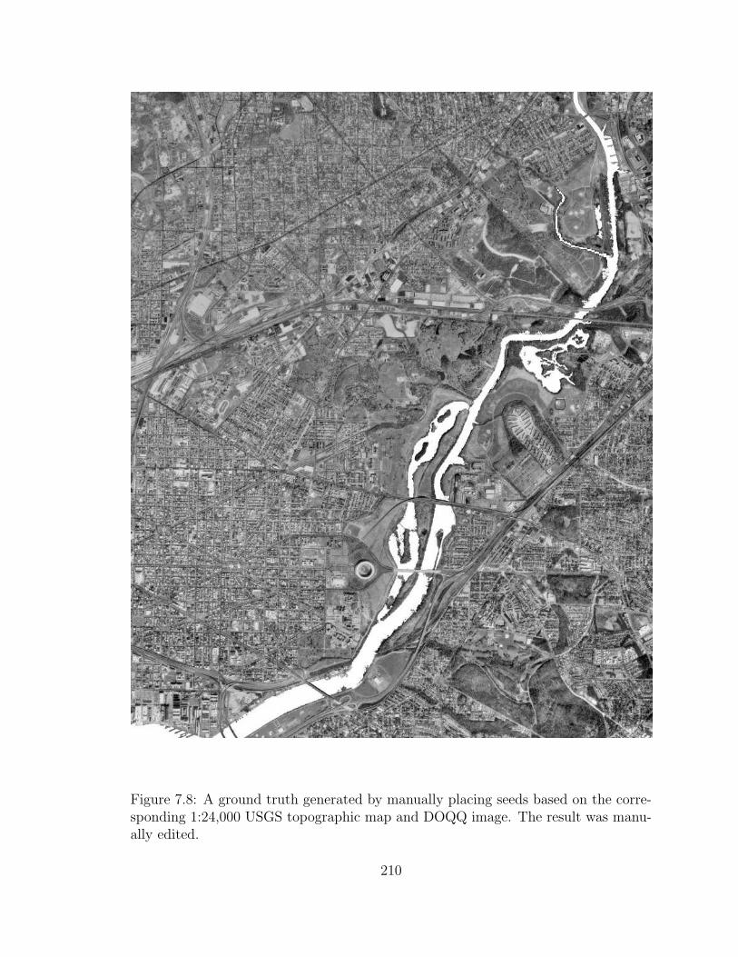
Figure 7.8: A ground truth generated by manually placing seeds based on the corre-sponding 1:24,000 USGS topographic map and DOQQ image. The result was manu-ally edited.
210
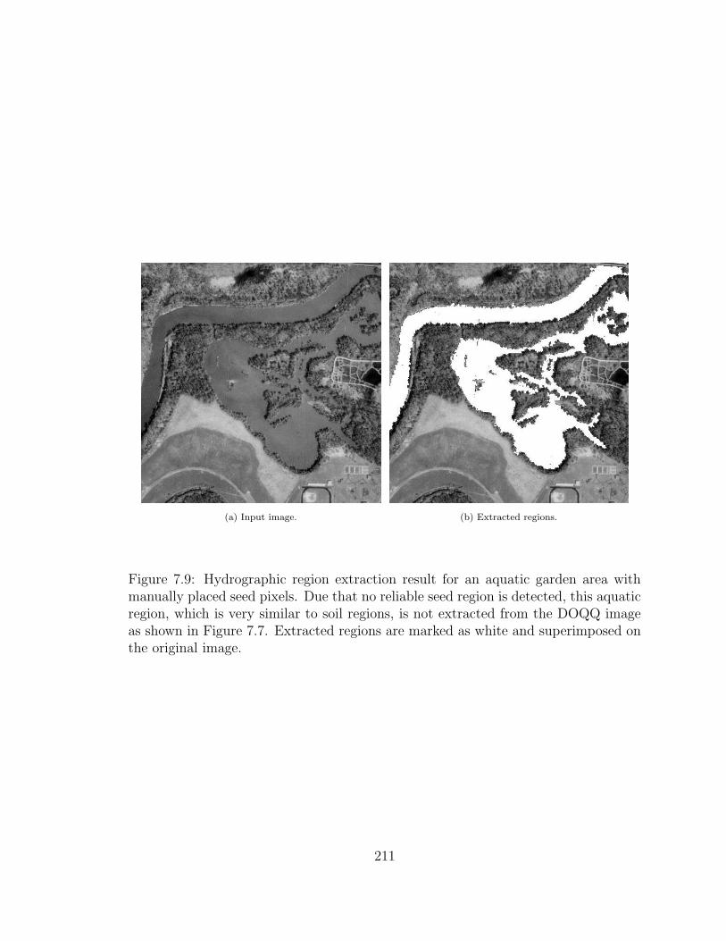
(a) Input image. (b) Extracted regions.
Figure 7.9: Hydrographic region extraction result for an aquatic garden area withmanually placed seed pixels. Due that no reliable seed region is detected, this aquaticregion, which is very similar to soil regions, is not extracted from the DOQQ imageas shown in Figure 7.7. Extracted regions are marked as white and superimposed onthe original image.
211
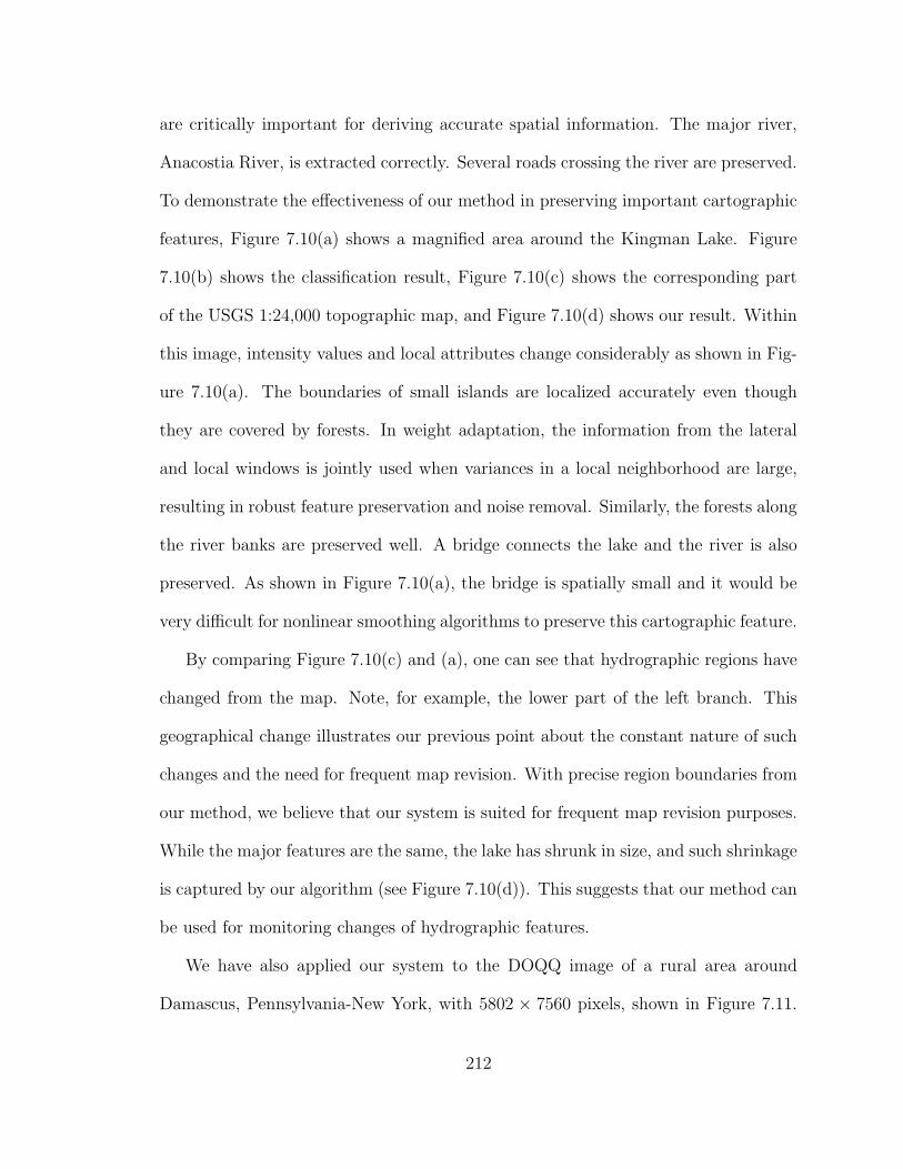
are critically important for deriving accurate spatial information. The major river,
Anacostia River, is extracted correctly. Several roads crossing the river are preserved.
To demonstrate the effectiveness of our method in preserving important cartographic
features, Figure 7.10(a) shows a magnified area around the Kingman Lake. Figure
7.10(b) shows the classification result, Figure 7.10(c) shows the corresponding part
of the USGS 1:24,000 topographic map, and Figure 7.10(d) shows our result. Within
this image, intensity values and local attributes change considerably as shown in Fig-
ure 7.10(a). The boundaries of small islands are localized accurately even though
they are covered by forests. In weight adaptation, the information from the lateral
and local windows is jointly used when variances in a local neighborhood are large,
resulting in robust feature preservation and noise removal. Similarly, the forests along
the river banks are preserved well. A bridge connects the lake and the river is also
preserved. As shown in Figure 7.10(a), the bridge is spatially small and it would be
very difficult for nonlinear smoothing algorithms to preserve this cartographic feature.
By comparing Figure 7.10(c) and (a), one can see that hydrographic regions have
changed from the map. Note, for example, the lower part of the left branch. This
geographical change illustrates our previous point about the constant nature of such
changes and the need for frequent map revision. With precise region boundaries from
our method, we believe that our system is suited for frequent map revision purposes.
While the major features are the same, the lake has shrunk in size, and such shrinkage
is captured by our algorithm (see Figure 7.10(d)). This suggests that our method can
be used for monitoring changes of hydrographic features.
We have also applied our system to the DOQQ image of a rural area around
Damascus, Pennsylvania-New York, with 5802 × 7560 pixels, shown in Figure 7.11.
212

(a) (b)
(c) (d)
Figure 7.10: Extraction result for an image patch from Figure 7.5. (a) The inputimage. (b) The seed points from the neural network. (c) A topographic map of thearea. Here the map is scanned from the chapter version and not wrapped with respectto the image. (d) Extracted result from the proposed method. Extracted regions arerepresented by white and superimposed on the original image.
213

Because this dataset is dramatically different from the Washington East dataset, the
multilayer perceptron is retrained using 25 positive and 17 negative training exam-
ples. Figure 7.12 shows the result from our method. Table 7.1 gives the quantitative
results from classification using the three-layer perceptron only and the proposed
method compared against a ground truth. Again, the ground truth, shown in Figure
7.13 is generated based on a 1:24,000 topographic map of the area. Generally speak-
ing, our extraction results for the Damascus image are comparable with those for the
Washington East image (In fact, a little better as revealed in Table 7.1). While the
major river, Delaware River, is extracted out with branches with great accuracy, and
small island features are preserved. However, a small river, the East Branch Calli-
coon Creek, located at upper right in the DOQQ image, is missing. When carefully
checking the DOQQ image, it is clear that the river is similar to its surrounding areas,
suggesting that the creek is not prominent.
To summarize, the results generated for both DOQQ images are comparable with
the hydrographic regions shown in the United States Geological Survey 1:24,000 to-
pographic maps. In certain cases, our results reflect better the current state of the
geographical areas.
By using a multilayer perceptron, characteristics of hydrographic regions are cap-
tured with only a small of number of training samples, even though there are consid-
erably variations within the regions. This greatly alleviates the problem of parameter
selection. For the DOQQ images shown here, only two parameters, namely Wz and θp,
need to be changed. This offers a distinctive advantage over many existing methods,
where extensive parameter tuning is needed.
214

Figure 7.11: A DOQQ image with size of 5802 × 7560 pixels of Damascus,Pennsylvania-New York area.
215
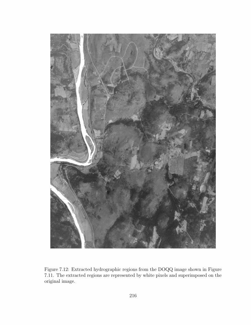
Figure 7.12: Extracted hydrographic regions from the DOQQ image shown in Figure7.11. The extracted regions are represented by white pixels and superimposed on theoriginal image.
216
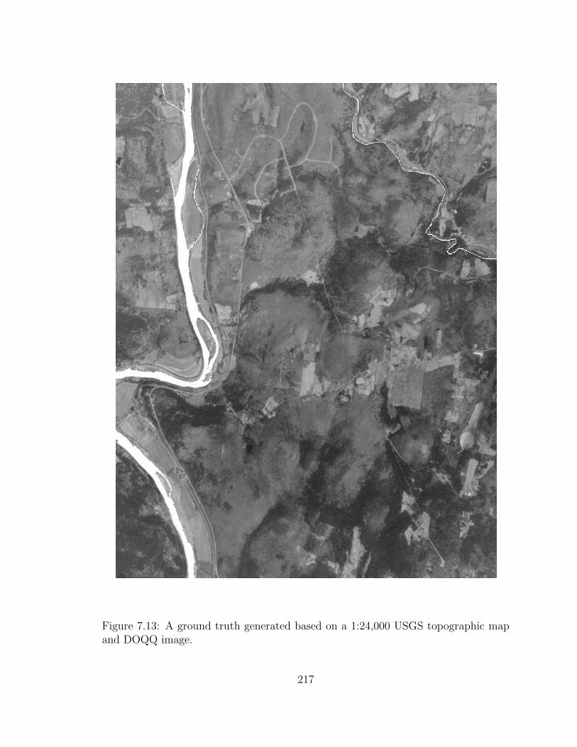
Figure 7.13: A ground truth generated based on a 1:24,000 USGS topographic mapand DOQQ image.
217
7.5 Discussions
In this chapter, we present a novel computational framework for extracting geo-
graphic features in general from remote sensing images. We demonstrate the feasibil-
ity of the method using hydrographic region extraction that is important for remote
sensing applications. By using LEGION as a segmentation framework, we combine
advantages of different methods. Using a multilayer perceptron, parameters can be
selected much more easily and the system can be adapted easily for other types of
features. Because multilayer perceptrons do not incorporate geometrical constraints
among neighboring pixels, we use a trained perceptron only for seed selection, which
determines the leaders in a LEGION network. We have used a weight adaptation
method to adaptively change local weights based on the statistical context provided
by a large window. This preserves major region boundaries while smoothing out
details due to variations and noise. It also preserves cartographic features such as
bridges and islands, which are important spatial information. Because geometric
constraints are incorporated in LEGION and weight adaptation, we achieve accurate
region boundaries. As shown by the numerical comparison, the proposed method
significantly improves the classification error from the multilayer perceptron.
Compared with existing classification approaches in remote sensing applications,
our method offers several advantages. By using the multilayer perceptron for seed se-
lection only, our method greatly improves generalization of the classification method
and reduces the number of necessary training samples. As shown in the experimental
results, the network is trained using only about 50 training samples and is successfully
applied to classify images with 6, 000× 8, 000 pixels. It would be very difficult, if not
218

impossible, to train a network to achieve results comparable to ours due to inconsis-
tency among different samples. Through weight adaptation, contextual information is
incorporated more efficiently and effectively. More importantly, our method extracts
boundaries that are comparable with features shown in topographic maps and thus
can be used for map revision purposes. To our knowledge, this is the only system
that is demonstrated for map revision using DOQQ images.
Practically, we demonstrate through a prototype system that hydrographic fea-
tures can be extracted highly automatically from DOQQ images. We have applied the
system to several DOQQ images and have obtained good results. With advances in
computing technology, very affordable systems can be built for map revision and other
feature extraction tasks. Compared with traditional map-making methods based on
aerial photogrammetry, our method is computationally efficient. We believe that this
kind of technology would be very useful for improving map revision and other remote
sensing applications. Further more, because remotely sensed images can be captured
more readily with high resolutions, efficient methods like the one proposed here are
necessary for generating up-to-date and accurate geographic information.
There are a number of improvements that can be made for our prototype system.
In the current version, features are extracted based on a single input image. While
good results have been obtained, they can be further improved by using data from
multiple sources. Feature extraction from multiple data sources has been studied
extensively [3] [118] [2]. Our method can potentially be applied to feature extraction
from multiple data sources. One possible way is to extend weight adaptation to vector
data by viewing the data from different sources in a vector form. A similar extension
has been done for nonlinear smoothing techniques [139]. Another constraint that is
219

not utilized is the relationships among different features; for example, when a road
crosses a river, there should be a bridge. In general, the knowledge concerning differ-
ent features can provide contextual information at a higher level than that currently
incorporated in our system. With these improvements, a complete feature extraction
system could be feasible.
220

CHAPTER 8
CONCLUSIONS AND FUTURE WORK
8.1 Contributions of Dissertation
This dissertation has investigated computational issues at different levels of image
organization and the major contributions are:
• We propose a new similarity for range images and implement a range image
segmentation system using a LEGION network.
• We propose a contextual nonlinear smoothing algorithm and show that several
widely used nonlinear smoothing algorithms are special cases. The proposed
algorithm generates quantitatively better results and exhibits nice properties
such as quick convergence.
• We propose the spectral histogram as a generic statistic feature for texture as
well as intensity images.
• We study image classification using the spectral histogram. We show that mean
and variance as statistical features are not sufficient and the distribution of
features is critically important for classification and segmentation.
221

• We propose a new energy function for image segmentation which expresses
explicitly the homogeneity criteria for segmentation. We implement an approx-
imate deterministic algorithm for image segmentation.
• We propose a method which can detect homogeneous texture regions in an input
image using the relationships between different scales.
• We propose a novel method for precise texture boundary localization utilizing
the structures of textures.
• We propose a boundary-pair representation and figure-ground segregation net-
work using temporal dynamics for perceptual organization.
• We propose a new computational framework for extracting features from re-
mote sensing images by combining the advantages of the learning-by-example
methods and locally coupled oscillator networks for better boundary accuracy.
8.2 Future Work
8.2.1 Correspondence Through Spectral Histograms
Two major areas in computer vision that are not addressed in this dissertation are
stereo matching and motion analysis. The central issue underlying both problems is
how to establish correspondence between input images, known as the correspondence
problem. We argue that the spectral histogram with the associated similarity measure
would potentially provide a solution to the correspondence problem. Because the
spectral histogram implicitly encodes the structures through marginal distributions,
it reduces matching ambiguities significantly compared to cross-correlation and other
feature-based matching techniques. For example, Figure 8.1 (a) and (b) show a stereo
222
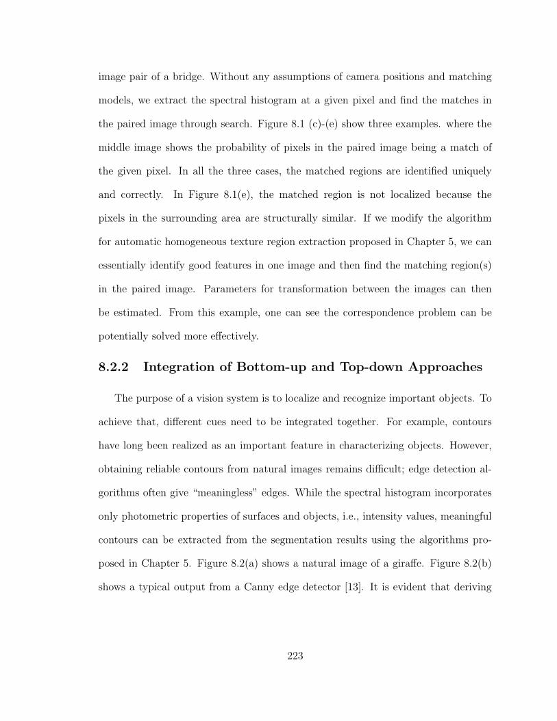
image pair of a bridge. Without any assumptions of camera positions and matching
models, we extract the spectral histogram at a given pixel and find the matches in
the paired image through search. Figure 8.1 (c)-(e) show three examples. where the
middle image shows the probability of pixels in the paired image being a match of
the given pixel. In all the three cases, the matched regions are identified uniquely
and correctly. In Figure 8.1(e), the matched region is not localized because the
pixels in the surrounding area are structurally similar. If we modify the algorithm
for automatic homogeneous texture region extraction proposed in Chapter 5, we can
essentially identify good features in one image and then find the matching region(s)
in the paired image. Parameters for transformation between the images can then
be estimated. From this example, one can see the correspondence problem can be
potentially solved more effectively.
8.2.2 Integration of Bottom-up and Top-down Approaches
The purpose of a vision system is to localize and recognize important objects. To
achieve that, different cues need to be integrated together. For example, contours
have long been realized as an important feature in characterizing objects. However,
obtaining reliable contours from natural images remains difficult; edge detection al-
gorithms often give “meaningless” edges. While the spectral histogram incorporates
only photometric properties of surfaces and objects, i.e., intensity values, meaningful
contours can be extracted from the segmentation results using the algorithms pro-
posed in Chapter 5. Figure 8.2(a) shows a natural image of a giraffe. Figure 8.2(b)
shows a typical output from a Canny edge detector [13]. It is evident that deriving
223
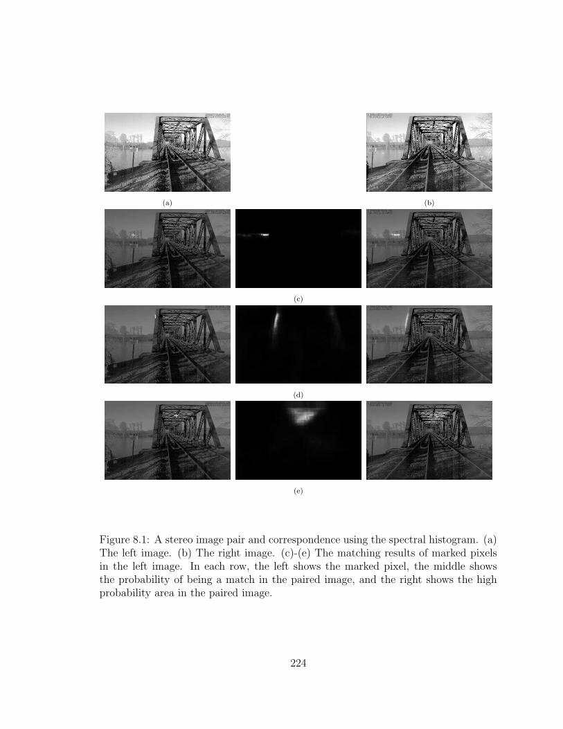
(a) (b)
(c)
(d)
(e)
Figure 8.1: A stereo image pair and correspondence using the spectral histogram. (a)The left image. (b) The right image. (c)-(e) The matching results of marked pixelsin the left image. In each row, the left shows the marked pixel, the middle showsthe probability of being a match in the paired image, and the right shows the highprobability area in the paired image.
224

a reliable contour from the generated edges is not feasible due to the local ambigu-
ities. Figure 8.2(c) shows an initial segmentation result using the method proposed
in Chapter 5. One can see that a contour of the giraffe can be obtained easily. This
demonstrates that features from bottom-up processes must be generic.
Of course, no one can expect a perfect segmentation and recognition result from
purely bottom-up algorithms. The top-down influence from recognition plays an
important role in achieving the purpose of a vision system. For example, an iterative
procedure can be initiated based on the result shown in Figure 8.2(c). In this case,
both the photometric properties and the contour may suggest a giraffe with high
probabilities. With the top-down knowledge, the segmentation result and contour
can be improved by recovering the missing parts of the giraffe.
There are important computational issues that need to be addressed in order to
model the interactions between bottom-up and top-down processes. In this regard,
temporal correlation with LEGION as a concrete implementation provides an elegant
representational framework. By utilizing temporal domain, LEGION provides dis-
tinctive advantages that are unique to dynamic systems and is biologically plausible.
The current model of LEGION [123] [134] [135] employs only very local couplings,
which significantly limits its potential. By incorporating longer-range and top-down
couplings, a complete vision system is conceivable. We have obtained very promising
results by integrating bottom-up and top-down processes [133], which is not included
in this dissertation.
225
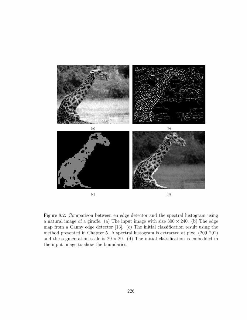
(a) (b)
(c) (d)
Figure 8.2: Comparison between en edge detector and the spectral histogram usinga natural image of a giraffe. (a) The input image with size 300× 240. (b) The edgemap from a Canny edge detector [13]. (c) The initial classification result using themethod presented in Chapter 5. A spectral histogram is extracted at pixel (209, 291)and the segmentation scale is 29 × 29. (d) The initial classification is embedded inthe input image to show the boundaries.
226
8.2.3 Psychophysical Experiments
While we claim that spectral histograms provide a generic feature for images and
have demonstrated that by synthesizing a wide range of texture images, including reg-
ular patterns, texton images, and many other natural images, rigorous psychophysical
experiments are needed to solidify the hypothesis. The result for texture discrimi-
nation discussed in Section 4.7 is very promising. However, the images used in the
experiment are synthetic and thus are not representative for natural images. One
straightforward experiment is to test on the correspondence between the observed
and synthesized images, as shown in Figure 4.16 and Figure 4.13. Another experi-
ment is to order a set of textures by humans as well as by an algorithm based on
spectral histograms. Other experiments can utilize the texture synthesis tool we have
to control the sharpness of texture boundaries and test on boundary accuracy and
asymmetry in texture perception.
Given all the results we have achieved using spectral histograms, some of which
match the human performance well, we would like to investigate if spectral histograms
are biologically plausible. It is well known that neurons encode information through
temporal spikes and spectral histograms can also be encoded very effectively that way
because spectral histograms can naturally be represented using temporal spikes. Also
the distance measure we used between two spectral histograms can be approximated
through cross correlations between them. As hypothesized by von der Malsburg [130],
temporal correlation provides a mechanism for solving fundamental problems in per-
ception such as feature binding. Spectral histograms would then extend significantly
the functionalities that can be achieved through temporal correlation.
227

8.3 Concluding Remarks
While developing a generic computational system for seeing remains the dream of
many vision researchers, significant progress can certainly be made by pursuing the
fundamental problems in a natural environment. Certainly there are many plausible
approaches for computer vision and the criterion to compare them is how efficient
vision tasks can be solved. Given the successful methods we have for relative inde-
pendent problems such as segmentation and pattern recognition, next steps would be
how to model the interactions among different modules and integrate them effectively
into a complete vision system. It is my sincere hope that this work would provide
some useful insights for solving the computer vision problems.
228

BIBLIOGRAPHY
[1] A. J. Bell and T. J. Sejnowski. “The “independent components” of naturalscenes are edge filters”. Vision Research, 37(23):3327–3338, 1997.
[2] J. A. Benediktsson and J. R. Sveinsson. “Feature extraction for multisourcedata classification with artificial neural networks”. International Journal onRemote Sensing, 18(4):727–740, March 1997.
[3] J. A. Benediktsson, P. H. Swain, and O. K. Ersoy. “Neural network approachesversus statistical methods in classification of multisource remote sensing data”.IEEE Transactions on Geoscience and Remote Sensing, 28(4):540–552, July1990.
[4] P. J. Besl and R. C. Jain. “Segmentation through variable-order surface fitting”.IEEE Transactions on Pattern Analysis and Machine Intelligence, 10(2):167–192, 1988.
[5] S. M. Bhandarkar, J. Koh, and M. Suk. “Multiscale image segmentation usinga hierarchical self-organizing map”. Neurocomputing, 14:241–272, 1997.
[6] B. Bhanu, S. Lee, C. C. Ho, and T. Henderson. “Range data processing: Rep-resentation of surfaces by edges”. In Proceedings of the IEEE InternationalPattern Recognition Conference, pages 236–238, 1986.
[7] I. Biederman. “Recognition-by-component: A theory of human image under-standing”. Psychological Review, 94(2):115–147, 1987.
[8] J. S. De Bonet and P. Viola. “A Non-parametric Multi-Scale Statistical Modelfor Natural Images”. In M. I. Jordan, M. J. Kearns, and S. A. Solla, editors,Advances in Neural Information Processing, volume 10, 1997.
[9] A. S. Bregman. Asking the ‘What for’ question in auditory perception. InM. Kubovy and J R. Pomerantz, editors, Perceptual Organization, pages 99–118. Lawrence Erlbaum Associates, Publishers, Hillsdale, New Jersey, 1981.
[10] P. Brodatz. Textures: A Photographic Album for Artists and Designers. DoverPublications, New York, 1966.
229
[11] T. Caelli, B. Julesz, and E. Gilbert. “On perceptual analyzers underlying visualtexture discrimination: Part II”. Biological Cybernetics, 29(4):201–214, 1978.
[12] F. W. Campbell and J. G. Robson. “Application of Fourier analysis to thevisibility of gratings”. Journal of Physiology (London), 197:551–566, 1968.
[13] J. Canny. “A computational approach to edge detection”. IEEE Transactionson Pattern Analysis and Machine Intelligence, 8(6):679–698, 1986.
[14] K. R. Castleman. Digital Image Processing. Prentice Hall, Englewood Cliffs,NJ, 1996.
[15] F. Catte, P.-L. Lions, J.-M. Morel, and T. Coll. “Image selective smoothing andedge detection by nonlinear diffusion”. SIAM Journal on Numerical Analysis,29:182–193, 1992.
[16] E. Cesmeli and D. L. Wang. “Texture segmentation using Gaussian Markovrandom fields and LEGION”. In Proceedings of the 1997 IEEE InternationalConference on Neural Networks, pages 1529–1534, 1997.
[17] K. Chen, D. L. Wang, and X. Liu. Weight adaptation and oscillatory cor-relation for image segmentation. Technical Report OSU-CISRC-8/98-TR37,Department of Computer and Information Science, The Ohio State University,1998.
[18] P. C. Chen and T. Pavlidis. “Segmentation by texture using correlation”. IEEETransactions on Pattern Recognition and Machine Intelligence, 5:64–69, 1983.
[19] M. A. Cohen and S. Grossberg. “Neural dynamics of brightness perception:features, boundaries, diffusion and resonance”. Perception and Psychophysics,36:428–456, 1984.
[20] T. H. Cormen, C. E. Leiserson, and R. L. Rivest. Introduction to Algorithms.MIT Press, Cambridge, MA, 1997.
[21] G. R. Cross and A. K. Jain. “Markov random field texture models”. IEEETransactions on Pattern Recognition and Machine Intelligence, 5:25–39, 1983.
[22] J. Daugman. “Uncertainty relation for resolution in space, spatial frequency,and orientation optimized by two-dimensional visual cortical filters”. Journalof the Optical Society of America A, 2(7):23–26, July 1985.
[23] R. L. De Valois and K. K. De Valois. Spatial Vision. Oxford University Press,New York, 1988.
230

[24] P. Diaconis and D. Freedman. “On the statistics of vision: the Julesz conjec-ture”. Journal of Mathematical Psychology, 24(2):112–138, 1981.
[25] R. O. Duda and P. E. Hart. Pattern Classification and Scene Analysis. JohnWiley and Sons, New York, 1973.
[26] R. Eckhorn, R. Bauer, W. Jordan, M. Brosch, W. Kruse, M. Munk, and H. J.Reitboeck. “Coherent oscillations: A mechanism of feature linking in the visualcortex?”. Biological Cybernetics, 60:121–130, 1988.
[27] R. Eckhorn, H. J. Reitboeck, M. Arndt, and P. Dicke. “Feature linking viasynchronization among distributed assemblies: Simulations of results from catvisual cortex”. Neural Computation, 2:293–307, 1990.
[28] T. F. El-Maraghi. An implementation of Heeger and Bergen’s textureanalysis/synthesis algorithm. Technical report, Department of ComputerScience, University of Toronto, Toronto, Ontario, 1998. (available athttp://www.cs.toronto.edu/∼tem/2522/texture.html).
[29] J. Elder and S. W. Zucker. Local scale control for edge detection and blurestimation. In Proceedings of the 4th European Conference on Computer Vision,volume II, pages 57–69. Springer Verlag, 1996.
[30] B. S. Everitt and D. J. Hand. Finite Mixture Distributions. Chapman and Hall,London, 1981.
[31] R. FitzHugh. “Impulses and physiological states in models of nerve membrane”.Biophysical Journal, 1:445–466, 1961.
[32] K. S. Fu and T. S. Yu. Statistical Pattern Classification using Contextual In-formation. Research Studies Press, Chichester, England, 1980.
[33] D. Gabor. “Theory of Communication”. Journal of IEE (London), 93:429–457,1946.
[34] D. Geiger, H. Pao, and N. Rubin. Salient and multiple illusory surfaces. InProceedings of IEEE Computer Society Conference on Computer Vision andPattern Recognition, pages 118–124, 1998.
[35] S. Geman and D. Geman. “Stochastic relaxation, Gibbs distributions and theBayesian restoration of images”. IEEE Transactions on Pattern Analysis andMachine Intelligence, 6(6):721–741, 1984.
[36] Z. Gigus and J. Malik. Detecting curvilinear structure in images. TechnicalReport Technical Report UCB/CSD 91/619, Computer Science Division, Uni-versity of California at Berkeley, 1991.
231
[37] C. D. Gillbert. “Horizontal integration and cortical dynamics”. Neuron, 9:1–13,1992.
[38] S. Gopal and C. Woodcock. “Remote sensing of forest change using artifi-cial neural networks”. IEEE Transactions on Geoscience and Remote Sensing,34(2):398–404, March 1996.
[39] B. Gorte and Alfred Stein. “Bayesian classification and class area estimationof satellite images using stratification”. IEEE Transactions on Geoscience andRemote Sensing, 36(3):803–812, May 1998.
[40] C. M. Gray, P. Konig, A. K. Engel, and W. Singer. “Oscillatory responses incat visual cortex exhibit inter-columnar synchronization which reflects globalstimulus properties”. Nature, 338:334–337, 1989.
[41] S. Grossberg and E. Mingolla. “Neural dynamics of perceptual grouping: Tex-tures, boundaries, and emergent segmentations”. Perception & Psychophysics,38(2):141–171, 1985.
[42] M. W. Hansen and W. E. Higgins. “Relaxation methods for supervised imagesegmentation”. IEEE Transactions on Pattern Analysis and Machine Intelli-gence, 19:949–962, 1997.
[43] R. M. Haralick. “Statistical and structural approach to texture”. Proceedingsof IEEE, 67:786–804, 1979.
[44] R. M. Haralick, K. Shanmugam, and I. Dinstein. “Texture features for im-age classification”. IEEE Transactions on Systems, Man, and Cybernetics,3(6):610–621, 1973.
[45] D. J. Heeger and J. R. Bergen. Pyramid-based texture analysis/synthesis. InProceedings of SIGGRAPHS, pages 229–238, 1995.
[46] J. Hertz, A. Krogh, and R. G. Palmer. Introduction to the Theory of NeuralComputation. Addison-Wesley, Reading, MA, 1991.
[47] W. E. Higgins and C. Hsu. “Edge detection using two-dimensional local struc-ture information”. Pattern Recognition, 27:277–294, 1994.
[48] A. L. Hodgkin and A. F. Huxley. “A quantitative description of membranecurrent and its application to conduction and excitation in nerve”. Journal ofPhysiology (London), 117:500–544, 1952.
[49] R. Hoffman and A. K. Jain. “Segmentation and classification of range images”.IEEE Transactions on Pattern Analysis and Machine Intelligence, 9(5):608–620, 1987.
232

[50] T. Hofmann, J. Puzicha, and J. M. Buhmann. “Unsupervised texture segmen-tation in a deterministic annealing framework.”. IEEE Transactions on PatternAnalysis and Machine Intelligence, 20(8):803–818, 1998.
[51] A. Hoover, G. Jean-Baptiste, X. Jiang, P. J. Flynn, H. Bunke, D. B. Goldgof,K. Bowyer, D. W. Eggert, A. Fitzgibbon, and R. B. Fisher. “An experimentalcomparison of range image segmentation algorithms”. IEEE Transactions onPattern Analysis and Machine Intelligence, 18(7):673–689, 1996.
[52] J. Y. Hsiao and A. A. Sawchuk. “Unsupervised textured image segmentationusing feature smoothing and probabilistic relaxation techniques”. ComputerVision, Graphics, and Image Processing, 48(1):1–21, 1989.
[53] D. H. Hubel. Eye, Brain, and Vision. W. H. Freeman and Company, New York,1988.
[54] D. H. Hubel and T. N. Wiesel. “Receptive fields, binocular interaction and func-tional architecture in the cat’s visual cortex”. Journal of Physiology (London),160:106–154, 1962.
[55] R. H. Hummel and S. W. Zucker. “On the foundations of relaxation labelingprocesses”. IEEE Transactions on Pattern Analysis and Machine Intelligence,5(3):267–286, 1983.
[56] D. J. Ittner and A. K. Jain. 3-D surface discrimination from local curvaturemeasures. In Proceedings of Computer Vision and Pattern Recognition Confer-ence, pages 119–123, 1985.
[57] Y. Jhung and P. H. Swain. “Bayesian contextual classification based on modifiedM-estimates and Markov Random Fields”. IEEE Transactions on Geoscienceand Remote Sensing, 34(1):67–75, January 1996.
[58] X. Y. Jiang and H. Bunke. “Fast segmentation of range images into planarregions by scan line grouping”. Machine Vision and Applications, 7(2):115–122, 1994.
[59] J. L. Johnson. “Pulse-coupled neural nets: translation, rotation, scale, distor-tion, and intensity signal invariance for images”. Applied Optics, 33(26):6239–6253, 1994.
[60] J. L. Johnson, M. L. Padgett, and W. A. Friday. Multiscale image factoriza-tion. In Proceedings of the IEEE International Conference on Neural Networks,volume 3, pages 1465–1468, 1997.
[61] B. Julesz. “A theory of preattentive texture discrimination based on first-orderstatistics of textons”. Biological Cybernetics, 41:131–138, 1962.
233

[62] B. Julesz. “Visual pattern discrimination”. IRE Transactions on InformationTheory, 8:84–92, 1962.
[63] B. Julesz. Dialogues on Perception. MIT Press, Cambridge, MA, 1995.
[64] G. Kanizsa. Quasi-perceptual margins in homogeneously stimulated fields. InS. Petry and G. E. Meyer, editors, The Perception of Illusory Contours, pages40–49. Springer-Verlag, New York, 1987.
[65] R. L. Kashyap, R. Chellappa, and A. Khotznzad. “Texture classification usingfeatures derived from random field models”. Pattern Recognition Letters, 1:43–50, 1982.
[66] J. Koenderink. “The structure of images”. Biological Cybernetics, 50:363–370,1984.
[67] J. Koh, M. Suk, and S. M. Bhandarkar. “A multilayer self-organizing featuremap for range image segmentation”. Neural Networks, 8(1):67–86, 1995.
[68] T. Kohonen. Self-Organizing Maps. Springer, Berlin, 1995.
[69] B. J. Krose. A description of visual structure. Ph.d. dissertation, Delft Univer-sity of Technology, Delft, The Netherlands, 1986.
[70] S. Kullback and R. A. Leibler. “On information and sufficiency”. Annals ofMathematical Statistics, 22:67–83, 1951.
[71] A. Leonardis, A. Gupta, and R. Bajcsy. Segmentation as the search for thebest description of the image in terms of primitives. In Proceedings of theInternational Conference on Computer Vision, pages 121–125, 1990.
[72] C. H. Li and C. K. Lee. “Image smoothing using parametric relaxation”. Graph-ical Models and Image Processing, 57:949–962, 1997.
[73] S. Z. Li. “Toward 3D vision from range images: An optimization framework andparallel networks”. Computer Vision, Graphics, and Image Processing: ImageUnderstanding, 55(3):231–260, 1992.
[74] T. Lindeberg and B. M. ter Haar Romeny. Linear scale-space. In B. M. terHaar Romeny, editor, Geometry-Driven Diffusion in Computer Vision, pages1–41. Kluwer Academic Publishers, Dordrecht, Netherlands, 19994.
[75] T. Linderberg. Scale-Space Theory in Computer Vision. Kluwer AcademicPublishers, Dordrecht, Netherlands, 1994.
234

[76] X. Liu. A prototype system for extracting hydrographic regions from DigitalOrthophoto Quadrangle images. In Proceedings of GIS/LIS’1998, pages 382–393, 1998.
[77] X. Liu, K. Chen, and D. L. Wang. “Extraction of hydrographic regions fromremote sensing images using an oscillator network with weight adaptation”.IEEE Transactions on Geoscience and Remote Sensing, under review.
[78] X. Liu and J. R. Ramirez. Automatic extraction of hydrographic features indigital orthophoto images. In GIS/LIS’1997, pages 365–373, 1997.
[79] X. Liu and D. Wang. Oriented Statistical Nonlinear Smoothing Filter. In Pro-ceedings of the 1998 International Conference on Image Processing, volume 2,pages 848–852, 1998.
[80] X. Liu, D. Wang, and J. R. Ramirez. “Boundary detection by contextual non-linear smoothing”. Pattern Recognition, in press.
[81] X. Liu and D. L. Wang. A boundary-pair representation for perception mod-eling. In Proceedings of the 1999 International Joint Conference on NeuralNetworks, 1999.
[82] X. Liu and D. L. Wang. Modeling perceptual organization using temporaldynamics. In Proceedings of the 1999 International Joint Conference on NeuralNetworks, 1999.
[83] X. Liu and D. L. Wang. “Range image segmentation using an oscillatory net-work”. IEEE Transactions on Neural Networks, 10(3):564–573, May 1999.
[84] X. Liu, D. L. Wang, and J. R. Ramirez. A two-layer neural network for ro-bust image segmentation and its application in revising hydrographic features.In International Archives of Photogrammetry and Remote Sensing, volume 32,pages 464–472, 1998.
[85] X. Liu, D. L. Wang, and J. R. Ramirez. Extracting hydrographic objects fromsatellite images using a two-layer neural network. In Proceedings of the 1998International Joint Conference on Neural Networks, volume 2, pages 897–902,1998.
[86] D. G. Lowe. Perceptual Organization and Visual Recognition. Academic Pub-lishers, Boston, 1985.
[87] J. Malik and P. Perona. “Preattentive texture discrimination with early visionmechanisms”. Journal of Optical Society of America A, 7(5):923–932, May1990.
235
[88] D. Marr. Vision: A computational investigation into the human representationand processing of visual information. W. H. Freeman and Company, New York,1982.
[89] D. Marr and E. Hildreth. “Theory of edge detection”. Proceedings of the RoyalSociety of London, Series B, 207:187–217, 1980.
[90] P. M. Milner. “A model for visual shape recognition”. Psychological Review,81(6):521–535, 1974.
[91] A. Mitiche and J. K. Aggarwal. “Detection of edges using range information”.IEEE Transactions on Pattern Analysis and Machine Intelligence, 5(2):174–178, 1983.
[92] J. M. Morel and S. Solimini. Variational Methods for Image Segmentation.Birkhauser, Boston, 1995.
[93] C. Morris and H. Lecar. “Voltage oscillations in the barnacle giant musclefiber”. Biophysical Journal, 35:193–213, 1981.
[94] D. Mumford and J. Shah. “Optimal approximations of piecewise smooth func-tions and associated variational problems”. Communications on Pure and Ap-plied Mathematics, XLII(4):577–685, 1989.
[95] M. Nagao and T. Matsuyama. “Edge preserving smoothing”. Computer Graph-ics and Image Processing, 9:394–407, 1979.
[96] J. Nagumo, S. Arimoto, and S. Yoshizawa. “An active pulse transmissionline simulating nerve axon”. Proceedings of the Institute of Radio Engineers,50:2061–2070, 1962.
[97] K. Nakayama, Z. J. He, and S. Shimojo. Visual surface representation: a criticallink between lower-level and higher-level vision. In S. M. Kosslyn and D. N.Osherson, editors, Visual Cognition, pages 1–70. The MIT Press, Cambridge,Massachusetts, 1995.
[98] M. Nitzberg, D. Mumford, and T. Shiota. Filtering, Segmentation and Depth.Springer-Verlag, 1994.
[99] T. Ojala, M. Pietikainen, and D. Harwood. “A comparative study of texturemeasures with classification based on feature distributions”. Pattern Recogni-tion, 29(1):51–59, 1996.
[100] B. A. Olshausen and D. J. Field. “Emergence of simple-cell receptive fieldproperties by learning a sparse code for natural images”. Nature, 381:607–609,1996.
236
[101] B. A. Olshausen and D. J. Field. “Natural image statitics and efficient coding”.Network, 7(2):333–340, 1996.
[102] B. A. Olshausen and D. J. Field. “Sparse coding with an overcomplete basisset: A strategy employed by V1?”. Vision Research, 37(23):3311–3325, 1997.
[103] M. L. Padgett and J. L. Johnson. Pulse coupled neural networks (PCNN)and wavelets: Biosensor applications. In Proceedings of the IEEE InternationalConference on Neural Networks, volume 4, pages 2507–2512, 1997.
[104] P. Perona. “Deformable kernels for early vision”. IEEE Transactions on PatternAnalysis and Machine Intelligence, 17:488–499, 1995.
[105] P. Perona and J. Malik. “Scale space and edge detection using anisotropicdiffusion”. IEEE Transactions on Pattern Analysis and Machine Intelligence,12:16–27, 1990.
[106] P. Perona, T. Shiota, and J. Malik. Anisotropic diffusion. In B. M. terHaar Romeny, editor, Geometry-Driven Diffusion in Computer Vision, pages73–92. Kluwer Academic Publishers, Dordrecht, Netherlands, 1994.
[107] J. Puzicha, T. Hofmann, and J. M. Buhmann. Non-parametric Similarity Mea-sures for Unsupervised Texture Segmentation and Image Retrieval. In Proceed-ings of the IEEE International Conference on Computer Vision and PatternRecognition, pages 267–272, 1997.
[108] T. Randen and J. H. Husoy. “Filtering for texture classification: A compara-tive study”. IEEE Transactions on Pattern Analysis and Machine Intelligence,21(4):291–310, April 1999.
[109] J. A. Richards. Remote Sensing Digital Image Analysis. Springer-Verlag, Berlin,1993.
[110] E. Rignot and R. Chellappa. “Segmentation of polarimetric synthetic apertureradar data”. IEEE Transactions on Image Processing, 1:281–300, July 1992.
[111] I. Rock and S. Palmer. “The legacy of Gestalt psychology”. Scientific American,263:84–90, 1990.
[112] A. Rosenfeld, R. A. Hummel, and S. W. Zucker. “Scene labeling by relaxationoperations”. IEEE Transactions on Systems, Man, and Cybernetics, 6(6):420–433, 1976.
[113] P. Saint-Marc, J.-S. Chen, and G. Medioni. “Adaptive smoothing: a generaltool for early vision”. IEEE Transactions on Pattern Analysis and MachineIntelligence, 13:514–529, 1991.
237
[114] S. Sarkar and K. L. Boyer. “On optimal infinite impulse response edge detec-tion filters”. IEEE Transactions on Pattern Analysis and Machine Intelligence,13:1154–1171, 1991.
[115] J. Schurmann. Pattern Classification: A Unified View of Statistical and NeuralApproaches. John Wiley and Sons, New York, 1996.
[116] W. Singer and C. M. Gray. “Visual feature integration and the temporal cor-relation hypothesis”. Annual Review of Neuroscience, 18:555–586, 1995.
[117] S. M. Smith and J. M. Brady. “SUSAN - a new approach to low level imageprocessing”. International Journal of Computer Vision, 23:45–78, 1997.
[118] A. H. S. Solberg, T. Taxt, and A. K. Jain. “A Markov Random Field modelfor classification of multisource satellite imagery”. IEEE Transactions on Geo-science and Remote Sensing, 34(1):100–113, January 1996.
[119] H. Stark and J. W. Woods. Probability, Random Processes and EstimationTheory for Engineers. Prentice-Hall, Englewood Cliffs, NJ, 1994.
[120] M. Stoecker, H. J. Reitboeck, and R. Eckhorn. “A neural network for scenesegmentation by temporal coding”. Neurocomputing, 11:123–134, 1996.
[121] C. Sun, C. M. U. Neale, J. J. McDonnell, and H. D. Cheng. “Monitoring land-surface snow conditions from SSM/I data using an artificial neural networkclassifier”. IEEE Transactions on Geoscience and Remote Sensing, 35(4):801–809, July 1997.
[122] M. Tabb and N. Ahuja. “Multiscale image segmentation by integrated edge andregion detection”. IEEE Transactions on Image Processing, 6:642–655, 1997.
[123] D. Terman and D. L. Wang. “Global competition and local cooperation in anetwork of neural oscillators”. Physica D, 81(1-2):148–176, 1995.
[124] A. N. Tikhonov and V. Y. Arsenin. Solutions of Ill-Posed Problems. Winston,Washington, D.C., 1977.
[125] F. Tomita and S. Tsuji. “Extraction of multiple regions by smoothing in selectedneighborhoods”. IEEE Transactions on Systems, Man, and Cybernetics, 7:107–109, 1977.
[126] D. Tsintikidis, J. L. Haferman, E. N. Anagnostou, W. F. Krajewski, and T. F.Smith. “A neural network approach to estimating rainfall from spacebornemicrowave data”. IEEE Transactions on Geoscience and Remote Sensing,35(5):1079–1093, September 1997.
238
[127] M. Unser. “Texture classification and segmentation using wavelet frames”.IEEE Transactions on Image Processing, 4(11):1549–1560, 1995.
[128] B. van der Pol. “On ‘relaxation oscillations’”. Philosophical Magazine,2(11):978–992, 1926.
[129] B. C. Vemuri, A. Mitiche, and J. K. Aggarwal. “Curvature-based representationof objects from range data”. Image and Vision Computing, 4(2):107–114, 1986.
[130] C. von der Malsburg. The Correlation Theory of Brain Function. InternalReport 81-2, Max-Planck-Institute for Biophysical Chemistry, 1981.
[131] D. C. C. Wang, A. H. Vagnucci, and C. C. Li. “Gradient inverse weightedsmoothing scheme and the evaluation of its performance”. Computer Graphicsand Image Processing, 15:167–181, 1981.
[132] D. L. Wang. Habituation. In M. A. Arbib, editor, The Handbook of BrainTheory and Neural Networks, pages 441–444. The MIT Press, Cambridge, Mas-sachusetts, 1995.
[133] D. L. Wang and X. Liu. “Scene analysis by integrating primitive segmentationand associate memory”. In preparation, 1999.
[134] D. L. Wang and D. Terman. “Locally excitatory globally inhibitory oscillatornetworks”. IEEE Transactions on Neural Networks, 6(1):283–286, 1995.
[135] D. L. Wang and D. Terman. “Image segmentation based on oscillatory correla-tion ”. Neural Computation, 9:805–836, 1997.
[136] M. A. Wani and B. G. Batchelor. “Edge-region-based segmentation of rangeimages”. IEEE Transactions on Pattern Analysis and Machine Intelligence,16(3):314–319, 1994.
[137] J. Weickert. Theoretical foundations of anisotropic diffusion in image process-ing. In W. Kropatsch, R. Klette, and F. Solina, editors, Theoretical Foundationsof Computer Vision, pages 231–236. Springer-Verlag, Wien, Austria, 1996.
[138] J. Weickert. A review of nonlinear diffusion filtering. In Proceedings of the FirstInternational Conference on Scale-Space, pages 3–28, 1997.
[139] R. Whitaker and G. Gerig. Vector-valued diffusion. In B. M. ter Haar Romeny,editor, Geometry-Driven Diffusion in Computer Vision, pages 93–134. KluwerAcademic Publishers, Dordrecht, Netherlands, 1994.
[140] D. Williams and B. Julesz. “Perceptual asymmetry in texture perception”.Proceedings of National Academy of Sciences, 89:6531–6534, July 1992.
239
[141] L. R. Williams and A. R. Hanson. “Perceptual completion of occluded surfaces”.Computer Vision and Image Understanding, 64:1–20, 1996.
[142] A. P. Witkin. Scale space filtering. In Proceedings of the Eighth InternationalConference on Artificial Intelligence, pages 1019–1021, 1983.
[143] Y. N. Wu and S. C. Zhu. “Equivalence of image ensembles and fundamentalbounds for texture discrimination”. Submitted to IEEE Transactions on PatternRecognition and Machine Intelligence, 1999.
[144] R. Yagel, D. Cohen, and A. Kaufman. Context sensitive normal estimationfor volume imaging. In N. M. Patrikalakis, editor, Scientific Visualization ofPhysical Phenomena, pages 211–234. Springer-Verlag, New York, 1991.
[145] Y. L. You, W. Xu, A. Tannenbaum, and M. Kaveh. “Behavioral analysis ofanisotropic diffusion in image processing”. IEEE Transactions on Image Pro-cessing, 5:1539–1553, 1996.
[146] S. C. Zhu. Embedding Gestalt laws in the Markov random fields. In IEEEComputer Society Workshop on Perceptual Organization in Computer Vision,1998.
[147] S. C. Zhu, X. Liu, and Y. N. Wu. “Statistics matching and model pursuitby efficient MCMC”. IEEE Transactions on Pattern Recognition and MachineIntelligence, in press, 1999.
[148] S. C. Zhu, Y. N. Wu, and D. Mumford. FRAME: Filters, random field andmaximum entropy. In Proceedings of the International Conference on ComputerVision and Pattern Recognition, pages 686–693, 1996.
[149] S. C. Zhu, Y. N. Wu, and D. Mumford. “Minimax entropy principles and its ap-plication to texture modeling”. Neural Computation, 9(8):1627–1660, November1997.
[150] S. C. Zhu, Y. N. Wu, and D. Mumford. “FRAME: Filters, random field andmaximum entropy - Towards a unified theory for texture modeling”. Interna-tional Journal of Computer Vision, 27(2):1–20, 1998.
[151] S. C. Zhu and A. Yuille. “Region competition: unifying snakes, region growing,and Bayes/MDL for multiband image segmentation”. IEEE Transactions onPattern Analysis and Machine Intelligence, 18:884–900, 1996.
[152] S. W. Zucker. “Region growing: Childhood and adolescence”. Computer Graph-ics and Image Processing, 5:382–399, 1976.
240


