J.1 Introduction J-2
J.2 Basic Techniques of Integer Arithmetic J-2
J.3 Floating Point J-13
J.4 Floating-Point Multiplication J-17
J.5 Floating-Point Addition J-21
J.6 Division and Remainder J-27
J.7 More on Floating-Point Arithmetic J-32
J.8 Speeding Up Integer Addition J-37
J.9 Speeding Up Integer Multiplication and Division J-44
J.10 Putting It All Together J-58
J.11 Fallacies and Pitfalls J-62
J.12 Historical Perspective and References J-62
Exercises J-68
JComputer Arithmetic 1
by David GoldbergXerox Palo Alto Research Center
The Fast drives out the Slow even if the Fast is wrong.
W. Kahan
J-2 ■ Appendix J Computer Arithmetic
Although computer arithmetic is sometimes viewed as a specialized part of CPUdesign, it is a very important part. This was brought home for Intel in 1994 whentheir Pentium chip was discovered to have a bug in the divide algorithm. Thisfloating-point flaw resulted in a flurry of bad publicity for Intel and also costthem a lot of money. Intel took a $300 million write-off to cover the cost ofreplacing the buggy chips.
In this appendix, we will study some basic floating-point algorithms, includ-ing the division algorithm used on the Pentium. Although a tremendous variety ofalgorithms have been proposed for use in floating-point accelerators, actualimplementations are usually based on refinements and variations of the few basicalgorithms presented here. In addition to choosing algorithms for addition, sub-traction, multiplication, and division, the computer architect must make otherchoices. What precisions should be implemented? How should exceptions behandled? This appendix will give you the background for making these and otherdecisions.
Our discussion of floating point will focus almost exclusively on the IEEEfloating-point standard (IEEE 754) because of its rapidly increasing acceptance.Although floating-point arithmetic involves manipulating exponents and shiftingfractions, the bulk of the time in floating-point operations is spent operating onfractions using integer algorithms (but not necessarily sharing the hardware thatimplements integer instructions). Thus, after our discussion of floating point, wewill take a more detailed look at integer algorithms.
Some good references on computer arithmetic, in order from least to mostdetailed, are Chapter 3 of Patterson and Hennessy [2009]; Chapter 7 of Ham-acher, Vranesic, and Zaky [1984]; Gosling [1980]; and Scott [1985].
Readers who have studied computer arithmetic before will find most of this sec-tion to be review.
Ripple-Carry Addition
Adders are usually implemented by combining multiple copies of simple com-ponents. The natural components for addition are half adders and full adders.The half adder takes two bits a and b as input and produces a sum bit s and acarry bit cout as output. Mathematically, s = (a + b) mod 2, and cout = ⎣(a + b)/2⎦, where ⎣ ⎦ is the floor function. As logic equations, s = ab + ab and cout = ab,where ab means a ∧ b and a + b means a ∨ b. The half adder is also called a(2,2) adder, since it takes two inputs and produces two outputs. The full adder
J.1 Introduction
J.2 Basic Techniques of Integer Arithmetic
J.2 Basic Techniques of Integer Arithmetic ■ J-3
is a (3,2) adder and is defined by s = (a + b + c) mod 2, cout = ⎣(a + b + c)/2⎦, orthe logic equations
J.2.1 s = ab c + abc + abc + abc
J.2.2 cout = ab + ac + bc
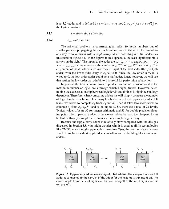
The principal problem in constructing an adder for n-bit numbers out ofsmaller pieces is propagating the carries from one piece to the next. The most obvi-ous way to solve this is with a ripple-carry adder, consisting of n full adders, asillustrated in Figure J.1. (In the figures in this appendix, the least-significant bit isalways on the right.) The inputs to the adder are an–1an–2 ⋅ ⋅ ⋅ a0 and bn–1bn–2 ⋅ ⋅ ⋅ b0,where an–1an–2 ⋅ ⋅ ⋅ a0 represents the number an–1 2n–1 + an–2 2n–2 + ⋅ ⋅ ⋅ + a0. Theci+1 output of the ith adder is fed into the ci+1 input of the next adder (the (i + 1)-thadder) with the lower-order carry-in c0 set to 0. Since the low-order carry-in iswired to 0, the low-order adder could be a half adder. Later, however, we will seethat setting the low-order carry-in bit to 1 is useful for performing subtraction.
In general, the time a circuit takes to produce an output is proportional to themaximum number of logic levels through which a signal travels. However, deter-mining the exact relationship between logic levels and timings is highly technologydependent. Therefore, when comparing adders we will simply compare the numberof logic levels in each one. How many levels are there for a ripple-carry adder? Ittakes two levels to compute c1 from a0 and b0. Then it takes two more levels tocompute c2 from c1, a1, b1, and so on, up to cn. So, there are a total of 2n levels.Typical values of n are 32 for integer arithmetic and 53 for double-precision float-ing point. The ripple-carry adder is the slowest adder, but also the cheapest. It canbe built with only n simple cells, connected in a simple, regular way.
Because the ripple-carry adder is relatively slow compared with the designsdiscussed in Section J.8, you might wonder why it is used at all. In technologieslike CMOS, even though ripple adders take time O(n), the constant factor is verysmall. In such cases short ripple adders are often used as building blocks in largeradders.
Figure J.1 Ripple-carry adder, consisting of n full adders. The carry-out of one fulladder is connected to the carry-in of the adder for the next most-significant bit. Thecarries ripple from the least-significant bit (on the right) to the most-significant bit(on the left).
bn–1
an–1
sn–1
Fulladder
cn–1
sn–2
cn
an–2
bn–2
Fulladder
b1
a1
s1
Fulladder
s0
a0
b0
Fulladder
c2 c
1
0
J-4 ■ Appendix J Computer Arithmetic
Radix-2 Multiplication and Division
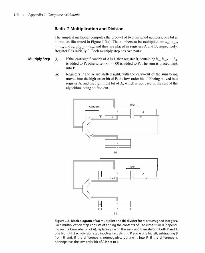
The simplest multiplier computes the product of two unsigned numbers, one bit ata time, as illustrated in Figure J.2(a). The numbers to be multiplied are an–1an–2⋅ ⋅ ⋅ a0 and bn–1bn–2 ⋅ ⋅ ⋅ b0, and they are placed in registers A and B, respectively.Register P is initially 0. Each multiply step has two parts:
Multiply Step (i) If the least-significant bit of A is 1, then register B, containing bn–1bn–2 ⋅ ⋅ ⋅ b0,is added to P; otherwise, 00 ⋅ ⋅ ⋅ 00 is added to P. The sum is placed backinto P.
(ii) Registers P and A are shifted right, with the carry-out of the sum beingmoved into the high-order bit of P, the low-order bit of P being moved intoregister A, and the rightmost bit of A, which is not used in the rest of thealgorithm, being shifted out.
Figure J.2 Block diagram of (a) multiplier and (b) divider for n-bit unsigned integers.Each multiplication step consists of adding the contents of P to either B or 0 (depend-ing on the low-order bit of A), replacing P with the sum, and then shifting both P and Aone bit right. Each division step involves first shifting P and A one bit left, subtracting Bfrom P, and, if the difference is nonnegative, putting it into P. If the difference isnonnegative, the low-order bit of A is set to 1.
Carry-out
P A
n
n
n
Shift
P
B0
A
n + 1
n1
n
Shift
(a)
(b)
1
B
J.2 Basic Techniques of Integer Arithmetic ■ J-5
After n steps, the product appears in registers P and A, with A holding thelower-order bits.
The simplest divider also operates on unsigned numbers and produces thequotient bits one at a time. A hardware divider is shown in Figure J.2(b). To com-pute a/b, put a in the A register, b in the B register, and 0 in the P register andthen perform n divide steps. Each divide step consists of four parts:
Divide Step (i) Shift the register pair (P,A) one bit left.
(ii) Subtract the content of register B (which is bn–1bn–2 ⋅ ⋅ ⋅ b0) from registerP, putting the result back into P.
(iii) If the result of step 2 is negative, set the low-order bit of A to 0, otherwiseto 1.
(iv) If the result of step 2 is negative, restore the old value of P by adding thecontents of register B back into P.
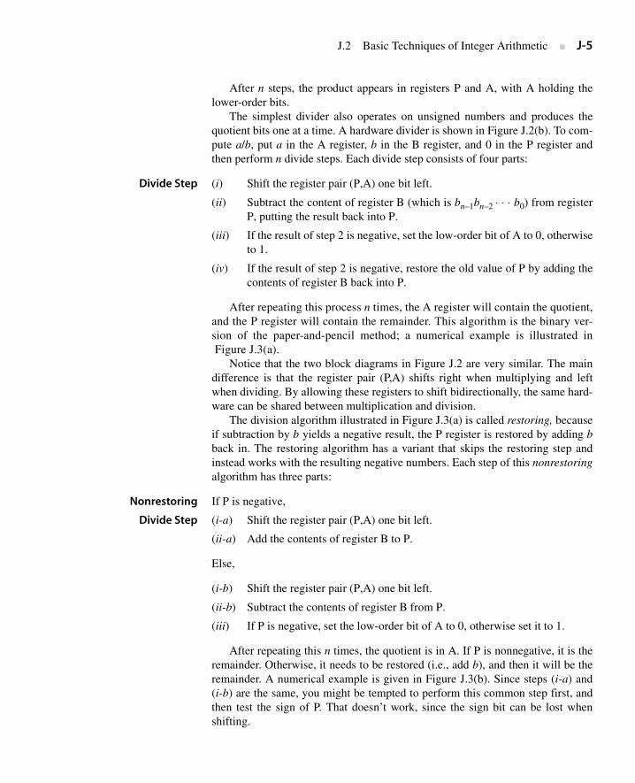
After repeating this process n times, the A register will contain the quotient,and the P register will contain the remainder. This algorithm is the binary ver-sion of the paper-and-pencil method; a numerical example is illustrated inFigure J.3(a).
Notice that the two block diagrams in Figure J.2 are very similar. The maindifference is that the register pair (P,A) shifts right when multiplying and leftwhen dividing. By allowing these registers to shift bidirectionally, the same hard-ware can be shared between multiplication and division.
The division algorithm illustrated in Figure J.3(a) is called restoring, becauseif subtraction by b yields a negative result, the P register is restored by adding bback in. The restoring algorithm has a variant that skips the restoring step andinstead works with the resulting negative numbers. Each step of this nonrestoringalgorithm has three parts:
Nonrestoring If P is negative,
Divide Step (i-a) Shift the register pair (P,A) one bit left.
(ii-a) Add the contents of register B to P.
Else,
(i-b) Shift the register pair (P,A) one bit left.
(ii-b) Subtract the contents of register B from P.
(iii) If P is negative, set the low-order bit of A to 0, otherwise set it to 1.
After repeating this n times, the quotient is in A. If P is nonnegative, it is theremainder. Otherwise, it needs to be restored (i.e., add b), and then it will be theremainder. A numerical example is given in Figure J.3(b). Since steps (i-a) and(i-b) are the same, you might be tempted to perform this common step first, andthen test the sign of P. That doesn’t work, since the sign bit can be lost whenshifting.
J-6 ■ Appendix J Computer Arithmetic
The explanation for why the nonrestoring algorithm works is this. Let rk bethe contents of the (P,A) register pair at step k, ignoring the quotient bits (whichare simply sharing the unused bits of register A). In Figure J.3(a), initially A con-tains 14, so r0 = 14. At the end of the first step, r1 = 28, and so on. In the restoring
Figure J.3 Numerical example of (a) restoring division and (b) nonrestoringdivision.
00000
00001
–00011
–00010
00001
00011
–00011
00000
00001
–00011
–00010
00001
00010
–00011
–00001
00010
1110
110
1100
1100
100
1001
001
0010
0010
010
0100
0100
Divide 14 = 11102 by 3 = 11
2. B always contains 0011
2.
step 1(i): shift.
step 1(ii): subtract.
step 1(iii): result is negative, set quotient bit to 0.
step 1(iv): restore.
step 2(i): shift.
step 2(ii): subtract.
P A
step 2(iii): result is nonnegative, set quotient bit to 1.
step 3(i): shift.
step 3(ii): subtract.
step 3(iii): result is negative, set quotient bit to 0.
step 3(iv): restore.
step 4(i): shift.
step 4(ii): subtract.
step 4(iii): result is negative, set quotient bit to 0.
step 4(iv): restore. The quotient is 01002 and the remainder is 00010
2.
00000
00001
+11101
11110
11101
+00011
00000
00001
+11101
11110
11100
+00011
11111
+00011
00010
1110
110
1100
100
1001
001
0010
010
0100
Divide 14 = 11102 by 3 = 11
2. B always contains 0011
2.
step 1(i-b): shift.
step 1(ii-b): subtract b (add two’s complement).
step 1(iii): P is negative, so set quotient bit to 0.
step 2(i-a): shift.
step 2(ii-a): add b.
step 2(iii): P is nonnegative, so set quotient bit to 1.
step 3(i-b): shift.
step 3(ii-b): subtract b.
step 3(iii): P is negative, so set quotient bit to 0.
step 4(i-a): shift.
step 4(ii-a): add b.
step 4(iii): P is negative, so set quotient bit to 0.
Remainder is negative, so do final restore step.
The quotient is 01002 and the remainder is 00010
2.
(b)
(a)
J.2 Basic Techniques of Integer Arithmetic ■ J-7
algorithm, part (i) computes 2rk and then part (ii) 2rk − 2nb (2nb since b is sub-tracted from the left half). If 2rk − 2nb ≥ 0, both algorithms end the step withidentical values in (P,A). If 2rk − 2nb < 0, then the restoring algorithm restoresthis to 2rk, and the next step begins by computing rres = 2(2rk) − 2nb. In the non-restoring algorithm, 2rk − 2nb is kept as a negative number, and in the next steprnonres = 2(2rk − 2nb) + 2nb = 4rk − 2nb = rres. Thus (P,A) has the same bits in bothalgorithms.
If a and b are unsigned n-bit numbers, hence in the range 0 ≤ a,b ≤ 2n − 1,then the multiplier in Figure J.2 will work if register P is n bits long. However, fordivision, P must be extended to n + 1 bits in order to detect the sign of P. Thus theadder must also have n + 1 bits.
Why would anyone implement restoring division, which uses the same hard-ware as nonrestoring division (the control is slightly different) but involves anextra addition? In fact, the usual implementation for restoring division doesn’tactually perform an add in step (iv). Rather, the sign resulting from the sub-traction is tested at the output of the adder, and only if the sum is nonnegative is itloaded back into the P register.
As a final point, before beginning to divide, the hardware must check to seewhether the divisor is 0.
Signed Numbers
There are four methods commonly used to represent signed n-bit numbers: signmagnitude, two’s complement, one’s complement, and biased. In the sign magni-tude system, the high-order bit is the sign bit, and the low-order n − 1 bits are themagnitude of the number. In the two’s complement system, a number and its neg-ative add up to 2n. In one’s complement, the negative of a number is obtained bycomplementing each bit (or, alternatively, the number and its negative add up to2n − 1). In each of these three systems, nonnegative numbers are represented inthe usual way. In a biased system, nonnegative numbers do not have their usualrepresentation. Instead, all numbers are represented by first adding them to thebias and then encoding this sum as an ordinary unsigned number. Thus, a nega-tive number k can be encoded as long as k + bias ≥ 0. A typical value for the biasis 2n–1.
Example Using 4-bit numbers (n = 4), if k = 3 (or in binary, k = 00112), how is −kexpressed in each of these formats?
Answer In signed magnitude, the leftmost bit in k = 00112 is the sign bit, so flip it to 1: −kis represented by 10112. In two’s complement, k + 11012 = 2n = 16. So −k is rep-resented by 11012. In one’s complement, the bits of k = 00112 are flipped, so −kis represented by 11002. For a biased system, assuming a bias of 2n−1 = 8, k isrepresented by k + bias = 10112, and −k by −k + bias = 01012.
J-8 ■ Appendix J Computer Arithmetic
The most widely used system for representing integers, two’s complement, isthe system we will use here. One reason for the popularity of two’s complementis that it makes signed addition easy: Simply discard the carry-out from the high-order bit. To add 5 + −2, for example, add 01012 and 11102 to obtain 00112,resulting in the correct value of 3. A useful formula for the value of a two’s com-plement number an–1an–2 ⋅ ⋅ ⋅ a1a0 is
J.2.3 −an–12n–1 + an–22n–2 + ⋅ ⋅ ⋅ + a121 + a0
As an illustration of this formula, the value of 11012 as a 4-bit two’s complementnumber is −1⋅23 + 1⋅22 + 0⋅21 + 1⋅20 = −8 + 4 + 1 = −3, confirming the result ofthe example above.
Overflow occurs when the result of the operation does not fit in the represen-tation being used. For example, if unsigned numbers are being represented using4 bits, then 6 = 01102 and 11 = 10112. Their sum (17) overflows because itsbinary equivalent (100012 ) doesn’t fit into 4 bits. For unsigned numbers, detect-ing overflow is easy; it occurs exactly when there is a carry-out of the most-significant bit. For two’s complement, things are trickier: Overflow occursexactly when the carry into the high-order bit is different from the (to be dis-carded) carry-out of the high-order bit. In the example of 5 + −2 above, a 1 is car-ried both into and out of the leftmost bit, avoiding overflow.
Negating a two’s complement number involves complementing each bit andthen adding 1. For instance, to negate 00112, complement it to get 11002 and thenadd 1 to get 11012. Thus, to implement a − b using an adder, simply feed a and b(where b is the number obtained by complementing each bit of b) into the adderand set the low-order, carry-in bit to 1. This explains why the rightmost adder inFigure J.1 is a full adder.
Multiplying two’s complement numbers is not quite as simple as addingthem. The obvious approach is to convert both operands to be nonnegative, do anunsigned multiplication, and then (if the original operands were of oppositesigns) negate the result. Although this is conceptually simple, it requires extratime and hardware. Here is a better approach: Suppose that we are multiplying atimes b using the hardware shown in Figure J.2(a). Register A is loaded with thenumber a; B is loaded with b. Since the content of register B is always b, we willuse B and b interchangeably. If B is potentially negative but A is nonnegative, theonly change needed to convert the unsigned multiplication algorithm into a two’scomplement one is to ensure that when P is shifted, it is shifted arithmetically;that is, the bit shifted into the high-order bit of P should be the sign bit of P(rather than the carry-out from the addition). Note that our n-bit-wide adder willnow be adding n-bit two’s complement numbers between −2n–1 and 2n–1 − 1.
Next, suppose a is negative. The method for handling this case is called Boothrecoding. Booth recoding is a very basic technique in computer arithmetic andwill play a key role in Section J.9. The algorithm on page J-4 computes a × b byexamining the bits of a from least significant to most significant. For example, ifa = 7 = 01112, then step (i) will successively add B, add B, add B, and add 0.Booth recoding “recodes” the number 7 as 8 − 1 = 10002 − 00012 = 1001, where
J.2 Basic Techniques of Integer Arithmetic ■ J-9
1 represents −1. This gives an alternative way to compute a × b, namely, succes-sively subtract B, add 0, add 0, and add B. This is more complicated than theunsigned algorithm on page J-4, since it uses both addition and subtraction. Theadvantage shows up for negative values of a. With the proper recoding, we cantreat a as though it were unsigned. For example, take a = −4 = 11002. Think of11002 as the unsigned number 12, and recode it as 12 = 16 − 4 = 100002 − 01002= 10100. If the multiplication algorithm is only iterated n times (n = 4 in thiscase), the high-order digit is ignored, and we end up subtracting 01002 = 4 timesthe multiplier—exactly the right answer. This suggests that multiplying using arecoded form of a will work equally well for both positive and negative numbers.And, indeed, to deal with negative values of a, all that is required is to sometimessubtract b from P, instead of adding either b or 0 to P. Here are the precise rules:If the initial content of A is an–1 ⋅ ⋅ ⋅ a0, then at the ith multiply step the low-orderbit of register A is ai , and step (i) in the multiplication algorithm becomes:
I. If ai = 0 and ai–1 = 0, then add 0 to P.
II. If ai = 0 and ai–1 = 1, then add B to P.
III. If ai = 1 and ai–1 = 0, then subtract B from P.
IV. If ai = 1 and ai–1 = 1, then add 0 to P.
For the first step, when i = 0, take ai–1 to be 0.
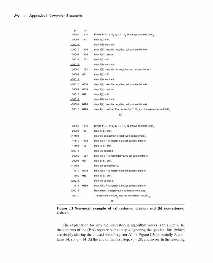
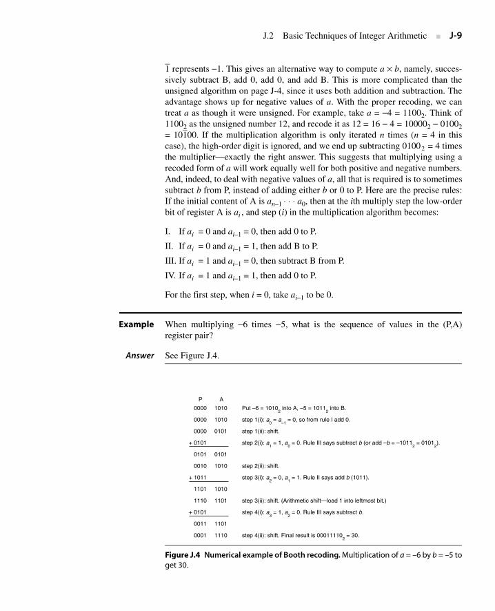
Example When multiplying −6 times −5, what is the sequence of values in the (P,A)register pair?
Answer See Figure J.4.
Figure J.4 Numerical example of Booth recoding. Multiplication of a = –6 by b = –5 toget 30.
0000
0000
0000
+ 0101
0101
0010
+ 1011
1101
1110
+ 0101
0011
0001
1010
1010
0101
0101
1010
1010
1101
1101
1110
Put –6 = 10102 into A, –5 = 1011
2 into B.
step 1(i): a0 = a
–1 = 0, so from rule I add 0.
step 1(ii): shift.
step 2(i): a1 = 1, a
0 = 0. Rule III says subtract b (or add –b = –1011
2 = 0101
2).
step 2(ii): shift.
step 3(i): a2 = 0, a
1 = 1. Rule II says add b (1011).
step 3(ii): shift. (Arithmetic shift—load 1 into leftmost bit.)
step 4(i): a3 = 1, a
2 = 0. Rule III says subtract b.
step 4(ii): shift. Final result is 000111102 = 30.
P A
J-10 ■ Appendix J Computer Arithmetic
The four prior cases can be restated as saying that in the ith step you shouldadd (ai–1 − ai )B to P. With this observation, it is easy to verify that these ruleswork, because the result of all the additions is
Using Equation J.2.3 (page J-8) together with a−1 = 0, the right-hand side is seento be the value of b × a as a two’s complement number.
The simplest way to implement the rules for Booth recoding is to extend the Aregister one bit to the right so that this new bit will contain ai–1. Unlike the naivemethod of inverting any negative operands, this technique doesn’t require extrasteps or any special casing for negative operands. It has only slightly more controllogic. If the multiplier is being shared with a divider, there will already be thecapability for subtracting b, rather than adding it. To summarize, a simple methodfor handling two’s complement multiplication is to pay attention to the sign of Pwhen shifting it right, and to save the most recently shifted-out bit of A to use indeciding whether to add or subtract b from P.
Booth recoding is usually the best method for designing multiplication hard-ware that operates on signed numbers. For hardware that doesn’t directly imple-ment it, however, performing Booth recoding in software or microcode is usuallytoo slow because of the conditional tests and branches. If the hardware supportsarithmetic shifts (so that negative b is handled correctly), then the followingmethod can be used. Treat the multiplier a as if it were an unsigned number, andperform the first n − 1 multiply steps using the algorithm on page J-4. If a < 0 (inwhich case there will be a 1 in the low-order bit of the A register at this point),then subtract b from P; otherwise (a ≥ 0), neither add nor subtract. In either case,do a final shift (for a total of n shifts). This works because it amounts to multiply-ing b by −an–1 2
n–1 + ⋅ ⋅ ⋅ + a12 + a0, which is the value of an–1 ⋅ ⋅ ⋅ a0 as a two’scomplement number by Equation J.2.3. If the hardware doesn’t support arithme-tic shift, then converting the operands to be nonnegative is probably the bestapproach.
Two final remarks: A good way to test a signed-multiply routine is to try−2n–1 × −2n–1, since this is the only case that produces a 2n − 1 bit result. Unlikemultiplication, division is usually performed in hardware by converting the oper-ands to be nonnegative and then doing an unsigned divide. Because division issubstantially slower (and less frequent) than multiplication, the extra time used tomanipulate the signs has less impact than it does on multiplication.
Systems Issues
When designing an instruction set, a number of issues related to integer arithme-tic need to be resolved. Several of them are discussed here.
First, what should be done about integer overflow? This situation is compli-cated by the fact that detecting overflow differs depending on whether the operands
b(ai 1– ai– )2i
i 0=
n 1–
∑ b an 1– 2n 1–
an 2– 2n 2–
. . . a12 a0+ + + +–( ) ba 1–+=
J.2 Basic Techniques of Integer Arithmetic ■ J-11
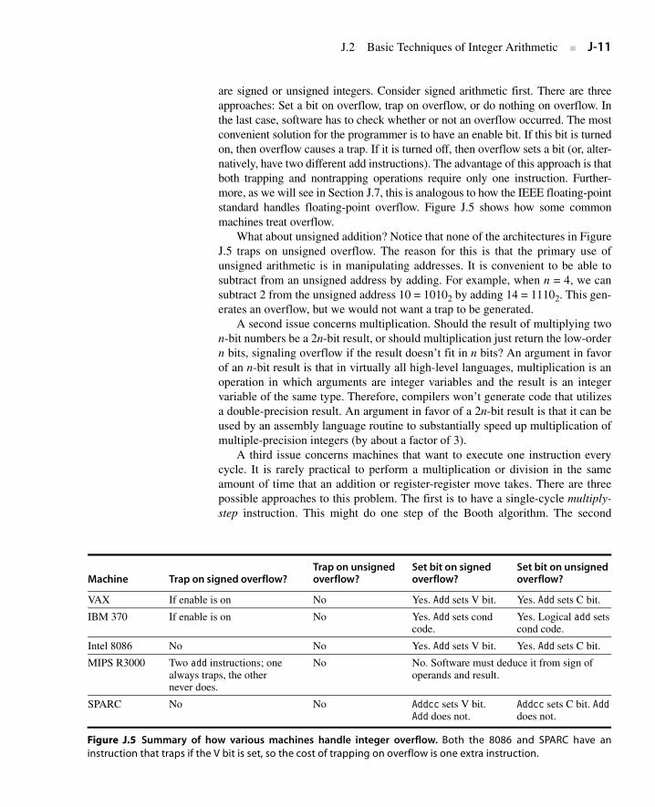
are signed or unsigned integers. Consider signed arithmetic first. There are threeapproaches: Set a bit on overflow, trap on overflow, or do nothing on overflow. Inthe last case, software has to check whether or not an overflow occurred. The mostconvenient solution for the programmer is to have an enable bit. If this bit is turnedon, then overflow causes a trap. If it is turned off, then overflow sets a bit (or, alter-natively, have two different add instructions). The advantage of this approach is thatboth trapping and nontrapping operations require only one instruction. Further-more, as we will see in Section J.7, this is analogous to how the IEEE floating-pointstandard handles floating-point overflow. Figure J.5 shows how some commonmachines treat overflow.
What about unsigned addition? Notice that none of the architectures in FigureJ.5 traps on unsigned overflow. The reason for this is that the primary use ofunsigned arithmetic is in manipulating addresses. It is convenient to be able tosubtract from an unsigned address by adding. For example, when n = 4, we cansubtract 2 from the unsigned address 10 = 10102 by adding 14 = 11102. This gen-erates an overflow, but we would not want a trap to be generated.
A second issue concerns multiplication. Should the result of multiplying twon-bit numbers be a 2n-bit result, or should multiplication just return the low-ordern bits, signaling overflow if the result doesn’t fit in n bits? An argument in favorof an n-bit result is that in virtually all high-level languages, multiplication is anoperation in which arguments are integer variables and the result is an integervariable of the same type. Therefore, compilers won’t generate code that utilizesa double-precision result. An argument in favor of a 2n-bit result is that it can beused by an assembly language routine to substantially speed up multiplication ofmultiple-precision integers (by about a factor of 3).
A third issue concerns machines that want to execute one instruction everycycle. It is rarely practical to perform a multiplication or division in the sameamount of time that an addition or register-register move takes. There are threepossible approaches to this problem. The first is to have a single-cycle multiply-step instruction. This might do one step of the Booth algorithm. The second
Machine Trap on signed overflow?Trap on unsigned overflow?
Set bit on signed overflow?
Set bit on unsigned overflow?
VAX If enable is on No Yes. Add sets V bit. Yes. Add sets C bit.
IBM 370 If enable is on No Yes. Add sets cond code.
Yes. Logical add setscond code.
Intel 8086 No No Yes. Add sets V bit. Yes. Add sets C bit.
MIPS R3000 Two add instructions; one always traps, the other never does.
No No. Software must deduce it from sign ofoperands and result.
SPARC No No Addcc sets V bit.Add does not.
Addcc sets C bit. Adddoes not.
Figure J.5 Summary of how various machines handle integer overflow. Both the 8086 and SPARC have aninstruction that traps if the V bit is set, so the cost of trapping on overflow is one extra instruction.
J-12 ■ Appendix J Computer Arithmetic
approach is to do integer multiplication in the floating-point unit and have it bepart of the floating-point instruction set. (This is what DLX does.) The thirdapproach is to have an autonomous unit in the CPU do the multiplication. In thiscase, the result either can be guaranteed to be delivered in a fixed number ofcycles—and the compiler charged with waiting the proper amount of time—orthere can be an interlock. The same comments apply to division as well. Asexamples, the original SPARC had a multiply-step instruction but no divide-stepinstruction, while the MIPS R3000 has an autonomous unit that does multiplica-tion and division (newer versions of the SPARC architecture added an integermultiply instruction). The designers of the HP Precision Architecture did anespecially thorough job of analyzing the frequency of the operands for multi-plication and division, and they based their multiply and divide steps accordingly.(See Magenheimer et al. [1988] for details.)
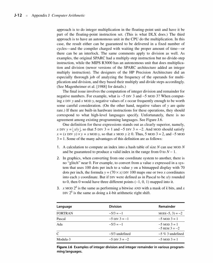
The final issue involves the computation of integer division and remainder fornegative numbers. For example, what is −5 DIV 3 and −5 MOD 3? When comput-ing x DIV y and x MOD y, negative values of x occur frequently enough to be worthsome careful consideration. (On the other hand, negative values of y are quiterare.) If there are built-in hardware instructions for these operations, they shouldcorrespond to what high-level languages specify. Unfortunately, there is noagreement among existing programming languages. See Figure J.6.
One definition for these expressions stands out as clearly superior, namely,x DIV y = ⎣x/y⎦, so that 5 DIV 3 = 1 and −5 DIV 3 = −2. And MOD should satisfyx = (x DIV y) × y + x MOD y, so that x MOD y ≥ 0. Thus, 5 MOD 3 = 2, and −5 MOD
3 = 1. Some of the many advantages of this definition are as follows:
1. A calculation to compute an index into a hash table of size N can use MOD Nand be guaranteed to produce a valid index in the range from 0 to N − 1.
2. In graphics, when converting from one coordinate system to another, there isno “glitch” near 0. For example, to convert from a value x expressed in a sys-tem that uses 100 dots per inch to a value y on a bitmapped display with 70dots per inch, the formula y = (70 × x) DIV 100 maps one or two x coordinatesinto each y coordinate. But if DIV were defined as in Pascal to be x/y roundedto 0, then 0 would have three different points (−1, 0, 1) mapped into it.
3. x MOD 2k is the same as performing a bitwise AND with a mask of k bits, and xDIV 2k is the same as doing a k-bit arithmetic right shift.
Language Division Remainder
FORTRAN −5/3 = −1 MOD(−5, 3) = −2
Pascal −5 DIV 3 = −1 −5 MOD 3 = 1
Ada −5/3 = −1 −5 MOD 3 = 1−5 REM 3 = −2
C −5/3 undefined −5 % 3 undefined
Modula-3 −5 DIV 3 = −2 −5 MOD 3 = 1
Figure J.6 Examples of integer division and integer remainder in various program-ming languages.
J.3 Floating Point ■ J-13
Finally, a potential pitfall worth mentioning concerns multiple-precisionaddition. Many instruction sets offer a variant of the add instruction that addsthree operands: two n-bit numbers together with a third single-bit number. Thisthird number is the carry from the previous addition. Since the multiple-precisionnumber will typically be stored in an array, it is important to be able to incrementthe array pointer without destroying the carry bit.
Many applications require numbers that aren’t integers. There are a number ofways that nonintegers can be represented. One is to use fixed point; that is, useinteger arithmetic and simply imagine the binary point somewhere other than justto the right of the least-significant digit. Adding two such numbers can be donewith an integer add, whereas multiplication requires some extra shifting. Otherrepresentations that have been proposed involve storing the logarithm of a num-ber and doing multiplication by adding the logarithms, or using a pair of integers(a,b) to represent the fraction a/b. However, only one noninteger representationhas gained widespread use, and that is floating point. In this system, a computerword is divided into two parts, an exponent and a significand. As an example, anexponent of −3 and a significand of 1.5 might represent the number 1.5 × 2–3
= 0.1875. The advantages of standardizing a particular representation are obvi-ous. Numerical analysts can build up high-quality software libraries, computerdesigners can develop techniques for implementing high-performance hardware,and hardware vendors can build standard accelerators. Given the predominanceof the floating-point representation, it appears unlikely that any other representa-tion will come into widespread use.
The semantics of floating-point instructions are not as clear-cut as the seman-tics of the rest of the instruction set, and in the past the behavior of floating-pointoperations varied considerably from one computer family to the next. The varia-tions involved such things as the number of bits allocated to the exponent and sig-nificand, the range of exponents, how rounding was carried out, and the actionstaken on exceptional conditions like underflow and overflow. Computer architec-ture books used to dispense advice on how to deal with all these details, but fortu-nately this is no longer necessary. That’s because the computer industry is rapidlyconverging on the format specified by IEEE standard 754-1985 (also an interna-tional standard, IEC 559). The advantages of using a standard variant of floatingpoint are similar to those for using floating point over other noninteger represen-tations.
IEEE arithmetic differs from many previous arithmetics in the followingmajor ways:
1. When rounding a “halfway” result to the nearest floating-point number, itpicks the one that is even.
2. It includes the special values NaN, ∞, and −∞.
J.3 Floating Point
J-14 ■ Appendix J Computer Arithmetic
3. It uses denormal numbers to represent the result of computations whose valueis less than 1.0 × 2Emin.
4. It rounds to nearest by default, but it also has three other rounding modes.
5. It has sophisticated facilities for handling exceptions.
To elaborate on (1), note that when operating on two floating-point numbers,the result is usually a number that cannot be exactly represented as another float-ing-point number. For example, in a floating-point system using base 10 and twosignificant digits, 6.1 × 0.5 = 3.05. This needs to be rounded to two digits. Shouldit be rounded to 3.0 or 3.1? In the IEEE standard, such halfway cases are roundedto the number whose low-order digit is even. That is, 3.05 rounds to 3.0, not 3.1.The standard actually has four rounding modes. The default is round to nearest,which rounds ties to an even number as just explained. The other modes areround toward 0, round toward +∞, and round toward –∞.
We will elaborate on the other differences in following sections. For furtherreading, see IEEE [1985], Cody et al. [1984], and Goldberg [1991].
Special Values and Denormals
Probably the most notable feature of the standard is that by default a computationcontinues in the face of exceptional conditions, such as dividing by 0 or takingthe square root of a negative number. For example, the result of taking the squareroot of a negative number is a NaN (Not a Number), a bit pattern that does notrepresent an ordinary number. As an example of how NaNs might be useful, con-sider the code for a zero finder that takes a function F as an argument and evalu-ates F at various points to determine a zero for it. If the zero finder accidentallyprobes outside the valid values for F, then F may well cause an exception. Writ-ing a zero finder that deals with this case is highly language and operating-systemdependent, because it relies on how the operating system reacts to exceptions andhow this reaction is mapped back into the programming language. In IEEE arith-metic it is easy to write a zero finder that handles this situation and runs on manydifferent systems. After each evaluation of F, it simply checks to see whether Fhas returned a NaN; if so, it knows it has probed outside the domain of F.
In IEEE arithmetic, if the input to an operation is a NaN, the output is NaN(e.g., 3 + NaN = NaN). Because of this rule, writing floating-point subroutinesthat can accept NaN as an argument rarely requires any special case checks. Forexample, suppose that arccos is computed in terms of arctan, using the formulaarccos x = 2 arctan( ). If arctan handles an argument of NaNproperly, arccos will automatically do so, too. That’s because if x is a NaN, 1 + x,1 − x, (1 + x)/(1 − x), and will also be NaNs. No checking forNaNs is required.
While the result of is a NaN, the result of 1/0 is not a NaN, but +∞, whichis another special value. The standard defines arithmetic on infinities (there are both
1 x–( ) 1 x+( )⁄
1 x–( ) 1 x+( )⁄
1–
J.3 Floating Point ■ J-15
+∞ and –∞) using rules such as 1/∞ = 0. The formula arccos x = 2 arc-tan( ) illustrates how infinity arithmetic can be used. Since arctanx asymptotically approaches π /2 as x approaches ∞, it is natural to define arctan(∞)= π/2, in which case arccos(−1) will automatically be computed correctly as 2 arc-tan(∞) = π.
The final kind of special values in the standard are denormal numbers. Inmany floating-point systems, if Emin is the smallest exponent, a number less than1.0 × 2Emin
cannot be represented, and a floating-point operation that results in anumber less than this is simply flushed to 0. In the IEEE standard, on the otherhand, numbers less than 1.0 × 2Emin are represented using significands less than 1.This is called gradual underflow. Thus, as numbers decrease in magnitude below2Emin, they gradually lose their significance and are only represented by 0 when alltheir significance has been shifted out. For example, in base 10 with foursignificant figures, let x = 1.234 × 10Emin. Then, x/10 will be rounded to 0.123 ×10Emin, having lost a digit of precision. Similarly x/100 rounds to 0.012 × 10Emin,and x/1000 to 0.001 × 10Emin, while x/10000 is finally small enough to be roundedto 0. Denormals make dealing with small numbers more predictable by maintain-ing familiar properties such as x = y ⇔ x − y = 0. For example, in a flush-to-zerosystem (again in base 10 with four significant digits), if x = 1.256 × 10Emin and y =1.234 × 10Emin, then x − y = 0.022 × 10Emin, which flushes to zero. So even thoughx ≠ y, the computed value of x − y = 0. This never happens with gradual underflow.In this example, x − y = 0.022 × 10Emin is a denormal number, and so the computa-tion of x − y is exact.
Representation of Floating-Point Numbers
Let us consider how to represent single-precision numbers in IEEE arithmetic.Single-precision numbers are stored in 32 bits: 1 for the sign, 8 for the exponent,and 23 for the fraction. The exponent is a signed number represented using thebias method (see the subsection “Signed Numbers,” page J-7) with a bias of 127.The term biased exponent refers to the unsigned number contained in bits 1through 8, and unbiased exponent (or just exponent) means the actual power towhich 2 is to be raised. The fraction represents a number less than 1, but the sig-nificand of the floating-point number is 1 plus the fraction part. In other words, ife is the biased exponent (value of the exponent field) and f is the value of the frac-tion field, the number being represented is 1. f × 2e–127.
Example What single-precision number does the following 32-bit word represent?
1 10000001 01000000000000000000000
Answer Considered as an unsigned number, the exponent field is 129, making the valueof the exponent 129 − 127 = 2. The fraction part is .012 = .25, making the signifi-cand 1.25. Thus, this bit pattern represents the number −1.25 × 22 = −5.
1 x–( ) 1 x+( )⁄
J-16 ■ Appendix J Computer Arithmetic
The fractional part of a floating-point number (.25 in the example above) mustnot be confused with the significand, which is 1 plus the fractional part. The lead-ing 1 in the significand 1. f does not appear in the representation; that is, the leadingbit is implicit. When performing arithmetic on IEEE format numbers, the fractionpart is usually unpacked, which is to say the implicit 1 is made explicit.
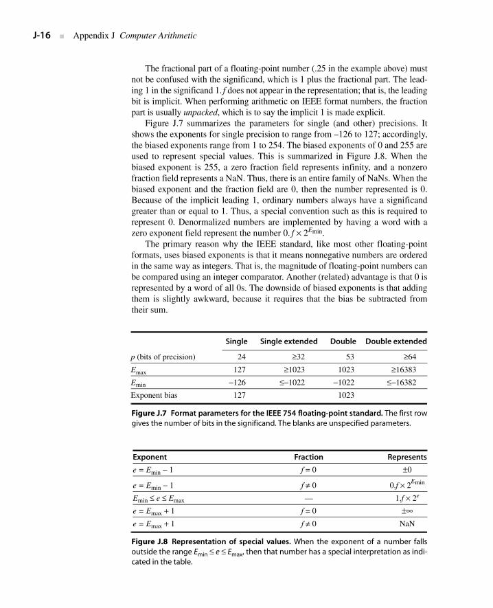
Figure J.7 summarizes the parameters for single (and other) precisions. Itshows the exponents for single precision to range from –126 to 127; accordingly,the biased exponents range from 1 to 254. The biased exponents of 0 and 255 areused to represent special values. This is summarized in Figure J.8. When thebiased exponent is 255, a zero fraction field represents infinity, and a nonzerofraction field represents a NaN. Thus, there is an entire family of NaNs. When thebiased exponent and the fraction field are 0, then the number represented is 0.Because of the implicit leading 1, ordinary numbers always have a significandgreater than or equal to 1. Thus, a special convention such as this is required torepresent 0. Denormalized numbers are implemented by having a word with azero exponent field represent the number 0. f × 2Emin.
The primary reason why the IEEE standard, like most other floating-pointformats, uses biased exponents is that it means nonnegative numbers are orderedin the same way as integers. That is, the magnitude of floating-point numbers canbe compared using an integer comparator. Another (related) advantage is that 0 isrepresented by a word of all 0s. The downside of biased exponents is that addingthem is slightly awkward, because it requires that the bias be subtracted fromtheir sum.
Single Single extended Double Double extended
p (bits of precision) 24 ≥32 53 ≥64
Emax 127 ≥1023 1023 ≥16383
Emin −126 ≤−1022 −1022 ≤−16382
Exponent bias 127 1023
Figure J.7 Format parameters for the IEEE 754 floating-point standard. The first rowgives the number of bits in the significand. The blanks are unspecified parameters.
Exponent Fraction Represents
e = Emin − 1 f = 0 ±0
e = Emin − 1 f ≠ 0 0.f × 2Emin
Emin ≤ e ≤ Emax — 1.f × 2e
e = Emax + 1 f = 0 ±∞e = Emax + 1 f ≠ 0 NaN
Figure J.8 Representation of special values. When the exponent of a number fallsoutside the range Emin ≤ e ≤ Emax, then that number has a special interpretation as indi-cated in the table.
J.4 Floating-Point Multiplication ■ J-17
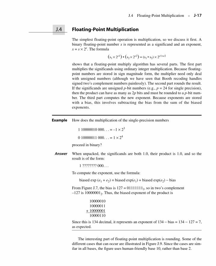
The simplest floating-point operation is multiplication, so we discuss it first. Abinary floating-point number x is represented as a significand and an exponent,x = s × 2e. The formula
(s1 × 2e1) • (s2 × 2e2) = (s1 • s2) × 2e1+e2
shows that a floating-point multiply algorithm has several parts. The first partmultiplies the significands using ordinary integer multiplication. Because floating-point numbers are stored in sign magnitude form, the multiplier need only dealwith unsigned numbers (although we have seen that Booth recoding handlessigned two’s complement numbers painlessly). The second part rounds the result.If the significands are unsigned p-bit numbers (e.g., p = 24 for single precision),then the product can have as many as 2p bits and must be rounded to a p-bit num-ber. The third part computes the new exponent. Because exponents are storedwith a bias, this involves subtracting the bias from the sum of the biasedexponents.
Example How does the multiplication of the single-precision numbers
1 10000010 000. . . = –1 × 23
0 10000011 000. . . = 1 × 24
proceed in binary?
Answer When unpacked, the significands are both 1.0, their product is 1.0, and so theresult is of the form:
1 ???????? 000. . .
To compute the exponent, use the formula:
biased exp (e1 + e2) = biased exp(e1) + biased exp(e2) − bias
From Figure J.7, the bias is 127 = 011111112, so in two’s complement –127 is 100000012. Thus, the biased exponent of the product is
10000010 10000011
+ 10000001 10000110
Since this is 134 decimal, it represents an exponent of 134 − bias = 134 − 127 = 7,as expected.
The interesting part of floating-point multiplication is rounding. Some of thedifferent cases that can occur are illustrated in Figure J.9. Since the cases are sim-ilar in all bases, the figure uses human-friendly base 10, rather than base 2.
J.4 Floating-Point Multiplication
J-18 ■ Appendix J Computer Arithmetic
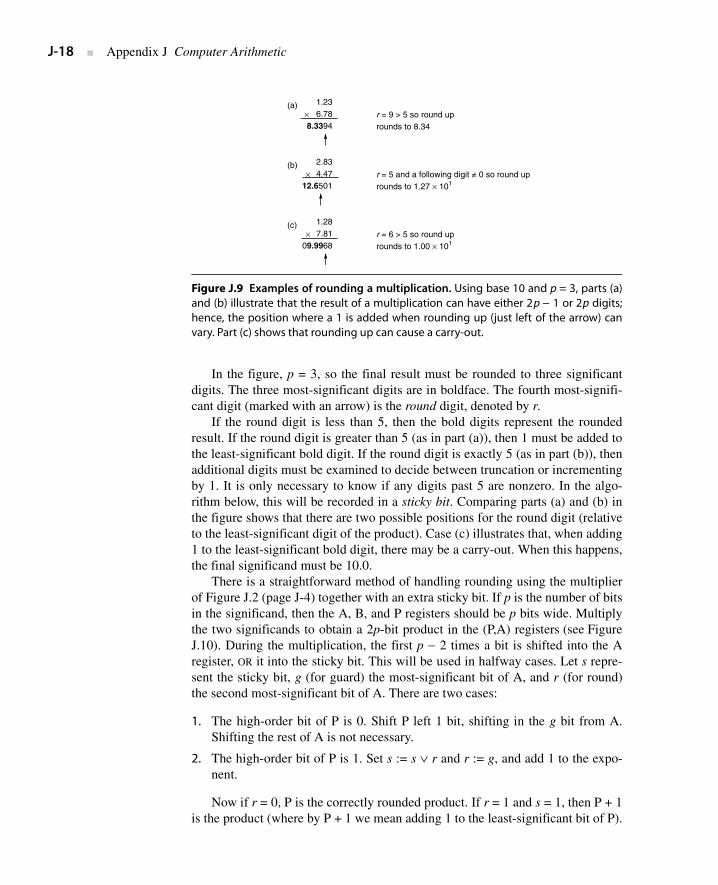
In the figure, p = 3, so the final result must be rounded to three significantdigits. The three most-significant digits are in boldface. The fourth most-signifi-cant digit (marked with an arrow) is the round digit, denoted by r.
If the round digit is less than 5, then the bold digits represent the roundedresult. If the round digit is greater than 5 (as in part (a)), then 1 must be added tothe least-significant bold digit. If the round digit is exactly 5 (as in part (b)), thenadditional digits must be examined to decide between truncation or incrementingby 1. It is only necessary to know if any digits past 5 are nonzero. In the algo-rithm below, this will be recorded in a sticky bit. Comparing parts (a) and (b) inthe figure shows that there are two possible positions for the round digit (relativeto the least-significant digit of the product). Case (c) illustrates that, when adding1 to the least-significant bold digit, there may be a carry-out. When this happens,the final significand must be 10.0.
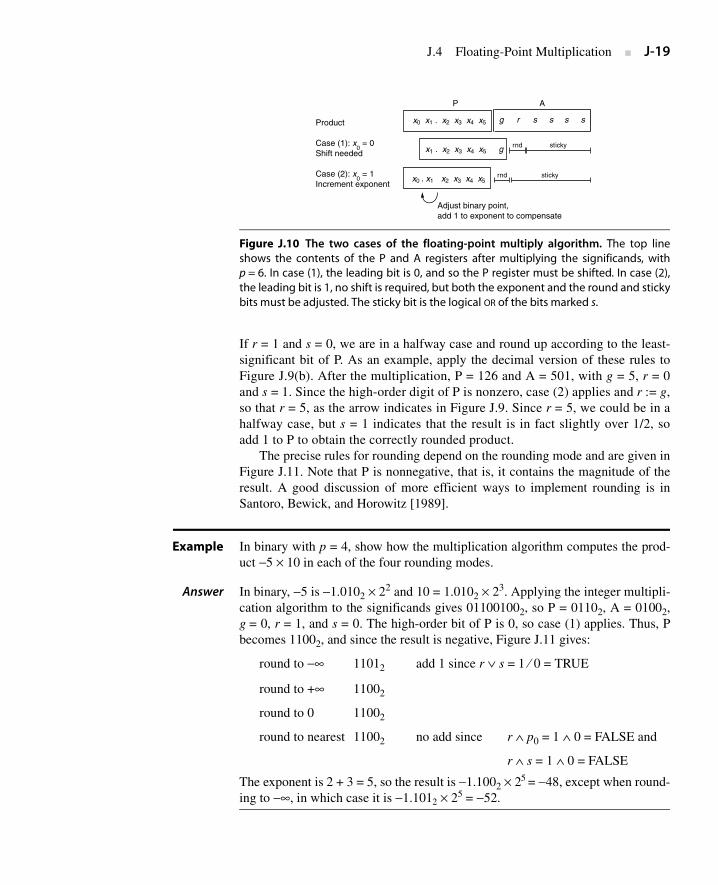
There is a straightforward method of handling rounding using the multiplierof Figure J.2 (page J-4) together with an extra sticky bit. If p is the number of bitsin the significand, then the A, B, and P registers should be p bits wide. Multiplythe two significands to obtain a 2p-bit product in the (P,A) registers (see FigureJ.10). During the multiplication, the first p − 2 times a bit is shifted into the Aregister, OR it into the sticky bit. This will be used in halfway cases. Let s repre-sent the sticky bit, g (for guard) the most-significant bit of A, and r (for round)the second most-significant bit of A. There are two cases:
1. The high-order bit of P is 0. Shift P left 1 bit, shifting in the g bit from A.Shifting the rest of A is not necessary.
2. The high-order bit of P is 1. Set s := s ∨ r and r := g, and add 1 to the expo-nent.
Now if r = 0, P is the correctly rounded product. If r = 1 and s = 1, then P + 1is the product (where by P + 1 we mean adding 1 to the least-significant bit of P).
Figure J.9 Examples of rounding a multiplication. Using base 10 and p = 3, parts (a)and (b) illustrate that the result of a multiplication can have either 2p − 1 or 2p digits;hence, the position where a 1 is added when rounding up (just left of the arrow) canvary. Part (c) shows that rounding up can cause a carry-out.
(a)
(b)
(c)
1.236.78
8.3394
2.834.47
12.6501
1.287.81
09.9968
r = 9 > 5 so round uprounds to 8.34
r = 5 and a following digit = 0 so round uprounds to 1.27 × 101
r = 6 > 5 so round uprounds to 1.00 × 101
×
×
×
J.4 Floating-Point Multiplication ■ J-19
If r = 1 and s = 0, we are in a halfway case and round up according to the least-significant bit of P. As an example, apply the decimal version of these rules toFigure J.9(b). After the multiplication, P = 126 and A = 501, with g = 5, r = 0and s = 1. Since the high-order digit of P is nonzero, case (2) applies and r := g,so that r = 5, as the arrow indicates in Figure J.9. Since r = 5, we could be in ahalfway case, but s = 1 indicates that the result is in fact slightly over 1/2, soadd 1 to P to obtain the correctly rounded product.
The precise rules for rounding depend on the rounding mode and are given inFigure J.11. Note that P is nonnegative, that is, it contains the magnitude of theresult. A good discussion of more efficient ways to implement rounding is inSantoro, Bewick, and Horowitz [1989].
Example In binary with p = 4, show how the multiplication algorithm computes the prod-uct −5 × 10 in each of the four rounding modes.
Answer In binary, −5 is −1.0102 × 22 and 10 = 1.0102 × 23. Applying the integer multipli-cation algorithm to the significands gives 011001002, so P = 01102, A = 01002,g = 0, r = 1, and s = 0. The high-order bit of P is 0, so case (1) applies. Thus, Pbecomes 11002, and since the result is negative, Figure J.11 gives:
round to −∞ 11012 add 1 since r ∨ s = 1 ⁄ 0 = TRUE
round to +∞ 11002
round to 0 11002
round to nearest 11002 no add since r ∧ p0 = 1 ∧ 0 = FALSE and
r ∧ s = 1 ∧ 0 = FALSE
The exponent is 2 + 3 = 5, so the result is −1.1002 × 25 = −48, except when round-
ing to −∞, in which case it is −1.1012 × 25 = −52.
Figure J.10 The two cases of the floating-point multiply algorithm. The top lineshows the contents of the P and A registers after multiplying the significands, withp = 6. In case (1), the leading bit is 0, and so the P register must be shifted. In case (2),the leading bit is 1, no shift is required, but both the exponent and the round and stickybits must be adjusted. The sticky bit is the logical OR of the bits marked s.
Product
Case (1): x0 = 0
Shift needed
Case (2): x0 = 1
Increment exponent
Adjust binary point,add 1 to exponent to compensate
rnd sticky
rnd sticky x2 x3 x4 x5x0 . x1
x1 . x2 x3 x4 x5 g
x0 x1 . x2 x3 x4 x5 g r ss s s
P A
J-20 ■ Appendix J Computer Arithmetic
Overflow occurs when the rounded result is too large to be represented. Insingle precision, this occurs when the result has an exponent of 128 or higher. Ife1 and e2 are the two biased exponents, then 1 ≤ ei ≤ 254, and the exponent calcu-lation e1 + e2 − 127 gives numbers between 1 + 1 − 127 and 254 + 254 − 127, orbetween −125 and 381. This range of numbers can be represented using 9 bits. Soone way to detect overflow is to perform the exponent calculations in a 9-bitadder (see Exercise J.12). Remember that you must check for overflow afterrounding—the example in Figure J.9(c) shows that this can make a difference.
Denormals
Checking for underflow is somewhat more complex because of denormals. In sin-gle precision, if the result has an exponent less than −126, that does not necessar-ily indicate underflow, because the result might be a denormal number. Forexample, the product of (1 × 2–64) with (1 × 2–65) is 1 × 2–129, and −129 is belowthe legal exponent limit. But this result is a valid denormal number, namely, 0.125× 2–126. In general, when the unbiased exponent of a product dips below −126, theresulting product must be shifted right and the exponent incremented until theexponent reaches −126. If this process causes the entire significand to be shiftedout, then underflow has occurred. The precise definition of underflow is some-what subtle—see Section J.7 for details.
When one of the operands of a multiplication is denormal, its significand willhave leading zeros, and so the product of the significands will also have leadingzeros. If the exponent of the product is less than –126, then the result is denormal,so right-shift and increment the exponent as before. If the exponent is greaterthan –126, the result may be a normalized number. In this case, left-shift theproduct (while decrementing the exponent) until either it becomes normalized orthe exponent drops to –126.
Denormal numbers present a major stumbling block to implementing floating-point multiplication, because they require performing a variable shift in themultiplier, which wouldn’t otherwise be needed. Thus, high-performance, float-ing-point multipliers often do not handle denormalized numbers, but instead trap,
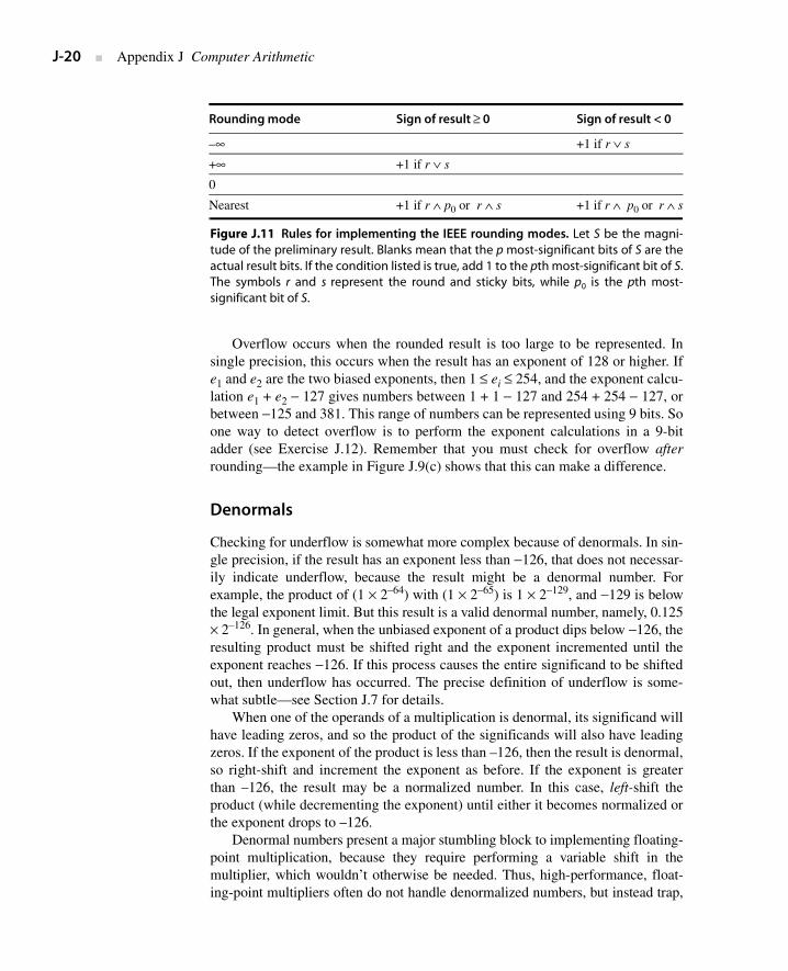
Rounding mode Sign of result ≥ 0 Sign of result < 0
–∞ +1 if r ∨ s
+∞ +1 if r ∨ s0
Nearest +1 if r ∧ p0 or r ∧ s +1 if r ∧ p0 or r ∧ s
Figure J.11 Rules for implementing the IEEE rounding modes. Let S be the magni-tude of the preliminary result. Blanks mean that the p most-significant bits of S are theactual result bits. If the condition listed is true, add 1 to the pth most-significant bit of S.The symbols r and s represent the round and sticky bits, while p0 is the pth most-significant bit of S.
J.5 Floating-Point Addition ■ J-21
letting software handle them. A few practical codes frequently underflow, evenwhen working properly, and these programs will run quite a bit slower on systemsthat require denormals to be processed by a trap handler.
So far we haven’t mentioned how to deal with operands of zero. This can behandled by either testing both operands before beginning the multiplication ortesting the product afterward. If you test afterward, be sure to handle the case0 × ∞ properly: This results in NaN, not 0. Once you detect that the result is 0, setthe biased exponent to 0. Don’t forget about the sign. The sign of a product is theXOR of the signs of the operands, even when the result is 0.
Precision of Multiplication
In the discussion of integer multiplication, we mentioned that designers mustdecide whether to deliver the low-order word of the product or the entire product.A similar issue arises in floating-point multiplication, where the exact productcan be rounded to the precision of the operands or to the next higher precision. Inthe case of integer multiplication, none of the standard high-level languages con-tains a construct that would generate a “single times single gets double” instruc-tion. The situation is different for floating point. Many languages allow assigningthe product of two single-precision variables to a double-precision one, and theconstruction can also be exploited by numerical algorithms. The best-known caseis using iterative refinement to solve linear systems of equations.
Typically, a floating-point operation takes two inputs with p bits of precision andreturns a p-bit result. The ideal algorithm would compute this by first performingthe operation exactly, and then rounding the result to p bits (using the currentrounding mode). The multiplication algorithm presented in the previous sectionfollows this strategy. Even though hardware implementing IEEE arithmetic mustreturn the same result as the ideal algorithm, it doesn’t need to actually performthe ideal algorithm. For addition, in fact, there are better ways to proceed. To seethis, consider some examples.
First, the sum of the binary 6-bit numbers 1.100112 and 1.100012 × 2–5:When the summands are shifted so they have the same exponent, this is
1.10011+ .0000110001
Using a 6-bit adder (and discarding the low-order bits of the second addend)gives
1.10011 + .00001
1.10100
J.5 Floating-Point Addition
J-22 ■ Appendix J Computer Arithmetic
The first discarded bit is 1. This isn’t enough to decide whether to round up. Therest of the discarded bits, 0001, need to be examined. Or, actually, we just need torecord whether any of these bits are nonzero, storing this fact in a sticky bit justas in the multiplication algorithm. So, for adding two p-bit numbers, a p-bit adderis sufficient, as long as the first discarded bit (round) and the OR of the rest of thebits (sticky) are kept. Then Figure J.11 can be used to determine if a roundup isnecessary, just as with multiplication. In the example above, sticky is 1, so aroundup is necessary. The final sum is 1.101012.
Here’s another example:
1.11011+ .0101001
A 6-bit adder gives:
1.11011+ .01010
10.00101
Because of the carry-out on the left, the round bit isn’t the first discarded bit;rather, it is the low-order bit of the sum (1). The discarded bits, 01, are OR’edtogether to make sticky. Because round and sticky are both 1, the high-order 6bits of the sum, 10.00102, must be rounded up for the final answer of 10.00112.
Next, consider subtraction and the following example:
1.00000– .00000101111
The simplest way of computing this is to convert −.000001011112 to its two’scomplement form, so the difference becomes a sum:
1.00000 + 1.11111010001
Computing this sum in a 6-bit adder gives:
1.00000 + 1.11111
0.11111
Because the top bits canceled, the first discarded bit (the guard bit) is needed tofill in the least-significant bit of the sum, which becomes 0.1111102, and the sec-ond discarded bit becomes the round bit. This is analogous to case (1) in the mul-tiplication algorithm (see page J-19). The round bit of 1 isn’t enough to decidewhether to round up. Instead, we need to OR all the remaining bits (0001) into asticky bit. In this case, sticky is 1, so the final result must be rounded up to0.111111. This example shows that if subtraction causes the most-significant bitto cancel, then one guard bit is needed. It is natural to ask whether two guard bits
J.5 Floating-Point Addition ■ J-23
are needed for the case when the two most-significant bits cancel. The answer isno, because if x and y are so close that the top two bits of x − y cancel, then x − ywill be exact, so guard bits aren’t needed at all.
To summarize, addition is more complex than multiplication because, depend-ing on the signs of the operands, it may actually be a subtraction. If it is an addition,there can be carry-out on the left, as in the second example. If it is subtraction, therecan be cancellation, as in the third example. In each case, the position of the roundbit is different. However, we don’t need to compute the exact sum and then round.We can infer it from the sum of the high-order p bits together with the round andsticky bits.
The rest of this section is devoted to a detailed discussion of the floating-point addition algorithm. Let a1 and a2 be the two numbers to be added. Thenotations ei and si are used for the exponent and significand of the addends ai.This means that the floating-point inputs have been unpacked and that si has anexplicit leading bit. To add a1 and a2, perform these eight steps:
1. If e1< e2, swap the operands. This ensures that the difference of the exponentssatisfies d = e1 − e2 ≥ 0. Tentatively set the exponent of the result to e1.
2. If the signs of a1 and a2 differ, replace s2 by its two’s complement.
3. Place s2 in a p-bit register and shift it d = e1 − e2 places to the right (shifting in1’s if s2 was complemented in the previous step). From the bits shifted out,set g to the most-significant bit, set r to the next most-significant bit, and setsticky to the OR of the rest.
4. Compute a preliminary significand S = s1 + s2 by adding s1 to the p-bit regis-ter containing s2. If the signs of a1 and a2 are different, the most-significantbit of S is 1, and there was no carry-out, then S is negative. Replace S with itstwo’s complement. This can only happen when d = 0.
5. Shift S as follows. If the signs of a1 and a2 are the same and there was a carry-out in step 4, shift S right by one, filling in the high-order position with 1 (thecarry-out). Otherwise, shift it left until it is normalized. When left-shifting, onthe first shift fill in the low-order position with the g bit. After that, shift inzeros. Adjust the exponent of the result accordingly.
6. Adjust r and s. If S was shifted right in step 5, set r := low-order bit of Sbefore shifting and s := g OR r OR s. If there was no shift, set r := g, s := r OR
s. If there was a single left shift, don’t change r and s. If there were two ormore left shifts, r := 0, s := 0. (In the last case, two or more shifts can onlyhappen when a1 and a2 have opposite signs and the same exponent, in whichcase the computation s1 + s2 in step 4 will be exact.)
7. Round S using Figure J.11; namely, if a table entry is nonempty, add 1 to thelow-order bit of S. If rounding causes carry-out, shift S right and adjust theexponent. This is the significand of the result.
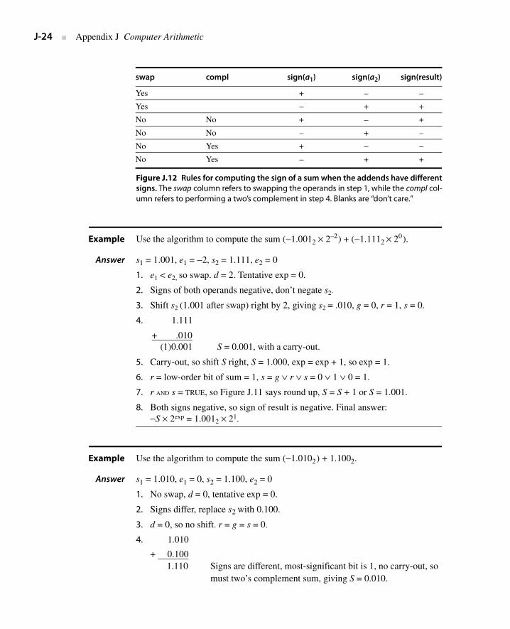
8. Compute the sign of the result. If a1 and a2 have the same sign, this is the signof the result. If a1 and a2 have different signs, then the sign of the result dependson which of a1 or a2 is negative, whether there was a swap in step 1, andwhether S was replaced by its two’s complement in step 4. See Figure J.12.
J-24 ■ Appendix J Computer Arithmetic
Example Use the algorithm to compute the sum (−1.0012 × 2–2) + (−1.1112 × 20).
Answer s1 = 1.001, e1 = −2, s2 = 1.111, e2 = 0
1. e1 < e2, so swap. d = 2. Tentative exp = 0.
2. Signs of both operands negative, don’t negate s2.
3. Shift s2 (1.001 after swap) right by 2, giving s2 = .010, g = 0, r = 1, s = 0.
4. 1.111
+ .010(1)0.001 S = 0.001, with a carry-out.
5. Carry-out, so shift S right, S = 1.000, exp = exp + 1, so exp = 1.
6. r = low-order bit of sum = 1, s = g ∨ r ∨ s = 0 ∨ 1 ∨ 0 = 1.
7. r AND s = TRUE, so Figure J.11 says round up, S = S + 1 or S = 1.001.
8. Both signs negative, so sign of result is negative. Final answer: −S × 2exp = 1.0012 × 21.
Example Use the algorithm to compute the sum (−1.0102) + 1.1002.
Answer s1 = 1.010, e1 = 0, s2 = 1.100, e2 = 0
1. No swap, d = 0, tentative exp = 0.
2. Signs differ, replace s2 with 0.100.
3. d = 0, so no shift. r = g = s = 0.
4. 1.010
+ 0.100 1.110 Signs are different, most-significant bit is 1, no carry-out, so
must two’s complement sum, giving S = 0.010.
swap compl sign(a1) sign(a2) sign(result)
Yes + – –
Yes – + +
No No + – +
No No – + –
No Yes + – –
No Yes – + +
Figure J.12 Rules for computing the sign of a sum when the addends have differentsigns. The swap column refers to swapping the operands in step 1, while the compl col-umn refers to performing a two’s complement in step 4. Blanks are “don’t care.”
J.5 Floating-Point Addition ■ J-25
5. Shift left twice, so S = 1.000, exp = exp − 2, or exp = −2.
6. Two left shifts, so r = g = s = 0.
7. No addition required for rounding.
8. Answer is sign × S × 2exp or sign × 1.000 × 2–2. Get sign from Figure J.12.Since complement but no swap and sign(a1) is −, the sign of the sum is +.Thus, the answer = 1.0002 × 2–2.
Speeding Up Addition
Let’s estimate how long it takes to perform the algorithm above. Step 2 mayrequire an addition, step 4 requires one or two additions, and step 7 may require anaddition. If it takes T time units to perform a p-bit add (where p = 24 for singleprecision, 53 for double), then it appears the algorithm will take at least 4T timeunits. But that is too pessimistic. If step 4 requires two adds, then a1 and a2have the same exponent and different signs, but in that case the difference is exact,so no roundup is required in step 7. Thus, only three additions will ever occur.Similarly, it appears that a variable shift may be required both in step 3 and step 5.But if |e1 − e2| ≤ 1, then step 3 requires a right shift of at most one place, so onlystep 5 needs a variable shift. And, if |e1 − e2| > 1, then step 3 needs a variable shift,but step 5 will require a left shift of at most one place. So only a single variableshift will be performed. Still, the algorithm requires three sequential adds, which,in the case of a 53-bit double-precision significand, can be rather time consuming.
A number of techniques can speed up addition. One is to use pipelining. The“Putting It All Together” section gives examples of how some commercial chipspipeline addition. Another method (used on the Intel 860 [Kohn and Fu 1989]) isto perform two additions in parallel. We now explain how this reduces the latencyfrom 3T to T.
There are three cases to consider. First, suppose that both operands have thesame sign. We want to combine the addition operations from steps 4 and 7.The position of the high-order bit of the sum is not known ahead of time, becausethe addition in step 4 may or may not cause a carry-out. Both possibilities areaccounted for by having two adders. The first adder assumes the add in step 4will not result in a carry-out. Thus, the values of r and s can be computed beforethe add is actually done. If r and s indicate that a roundup is necessary, the firstadder will compute S = s1 + s2 + 1, where the notation +1 means adding 1 at theposition of the least-significant bit of s1. This can be done with a regular adder bysetting the low-order carry-in bit to 1. If r and s indicate no roundup, the addercomputes S = s1 + s2 as usual. One extra detail: When r = 1, s = 0, you will alsoneed to know the low-order bit of the sum, which can also be computed inadvance very quickly. The second adder covers the possibility that there will becarry-out. The values of r and s and the position where the roundup 1 is added aredifferent from above, but again they can be quickly computed in advance. It is notknown whether there will be a carry-out until after the add is actually done, butthat doesn’t matter. By doing both adds in parallel, one adder is guaranteed toreduce the correct answer.
J-26 ■ Appendix J Computer Arithmetic
The next case is when a1 and a2 have opposite signs but the same exponent.The sum a1 + a2 is exact in this case (no roundup is necessary) but the sign isn’tknown until the add is completed. So don’t compute the two’s complement(which requires an add) in step 2, but instead compute s1 + s2 + 1 and s1 + s2 + 1in parallel. The first sum has the result of simultaneously complementing s1 andcomputing the sum, resulting in s2 − s1. The second sum computes s1 − s2. One ofthese will be nonnegative and hence the correct final answer. Once again, all theadditions are done in one step using two adders operating in parallel.
The last case, when a1 and a2 have opposite signs and different exponents, ismore complex. If |e1 − e2| > 1, the location of the leading bit of the difference is inone of two locations, so there are two cases just as in addition. When |e1 − e2| = 1,cancellation is possible and the leading bit could be almost anywhere. However,only if the leading bit of the difference is in the same position as the leading bit ofs1 could a roundup be necessary. So one adder assumes a roundup, and the otherassumes no roundup. Thus, the addition of step 4 and the rounding of step 7 canbe combined. However, there is still the problem of the addition in step 2!
To eliminate this addition, consider the following diagram of step 4:
|—— p ——|s1 1.xxxxxxxs2 – 1yyzzzzz
If the bits marked z are all 0, then the high-order p bits of S = s1 − s2 can be com-puted as s1 + s2 + 1. If at least one of the z bits is 1, use s1 + s2. So s1 − s2 can becomputed with one addition. However, we still don’t know g and r for the two’scomplement of s2, which are needed for rounding in step 7.
To compute s1 − s2 and get the proper g and r bits, combine steps 2 and 4 as fol-lows. Don’t complement s2 in step 2. Extend the adder used for computing S twobits to the right (call the extended sum S′). If the preliminary sticky bit (computedin step 3) is 1, compute S′ = s′1 + s ′2, where s′1 has two 0 bits tacked onto the right,and s′2 has preliminary g and r appended. If the sticky bit is 0, compute s′1 + s ′2 + 1.Now the two low-order bits of S′ have the correct values of g and r (the sticky bitwas already computed properly in step 3). Finally, this modification can be com-bined with the modification that combines the addition from steps 4 and 7 to pro-vide the final result in time T, the time for one addition.
A few more details need to be considered, as discussed in Santoro, Bewick,and Horowitz [1989] and Exercise J.17. Although the Santoro paper is aimed atmultiplication, much of the discussion applies to addition as well. Also relevantis Exercise J.19, which contains an alternative method for adding signed magni-tude numbers.
Denormalized Numbers
Unlike multiplication, for addition very little changes in the preceding descrip-tion if one of the inputs is a denormal number. There must be a test to see if theexponent field is 0. If it is, then when unpacking the significand there will not be
J.6 Division and Remainder ■ J-27
a leading 1. By setting the biased exponent to 1 when unpacking a denormal, thealgorithm works unchanged.
To deal with denormalized outputs, step 5 must be modified slightly. Shift Suntil it is normalized, or until the exponent becomes Emin (that is, the biasedexponent becomes 1). If the exponent is Emin and, after rounding, the high-orderbit of S is 1, then the result is a normalized number and should be packed in theusual way, by omitting the 1. If, on the other hand, the high-order bit is 0, theresult is denormal. When the result is unpacked, the exponent field must be set to0. Section J.7 discusses the exact rules for detecting underflow.
Incidentally, detecting overflow is very easy. It can only happen if step 5involves a shift right and the biased exponent at that point is bumped up to 255 insingle precision (or 2047 for double precision), or if this occurs after rounding.
In this section, we’ll discuss floating-point division and remainder.
Iterative Division
We earlier discussed an algorithm for integer division. Converting it into a float-ing-point division algorithm is similar to converting the integer multiplicationalgorithm into floating point. The formula
(s1 × 2e1) / (s2 × 2e2) = (s1 / s2) × 2e1–e2
shows that if the divider computes s1/s2, then the final answer will be this quo-tient multiplied by 2e1−e2. Referring to Figure J.2(b) (page J-4), the alignment ofoperands is slightly different from integer division. Load s2 into B and s1 into P.The A register is not needed to hold the operands. Then the integer algorithm fordivision (with the one small change of skipping the very first left shift) can beused, and the result will be of the form q0.q1
.... To round, simply compute twoadditional quotient bits (guard and round) and use the remainder as the sticky bit.The guard digit is necessary because the first quotient bit might be 0. However,since the numerator and denominator are both normalized, it is not possible forthe two most-significant quotient bits to be 0. This algorithm produces one quo-tient bit in each step.
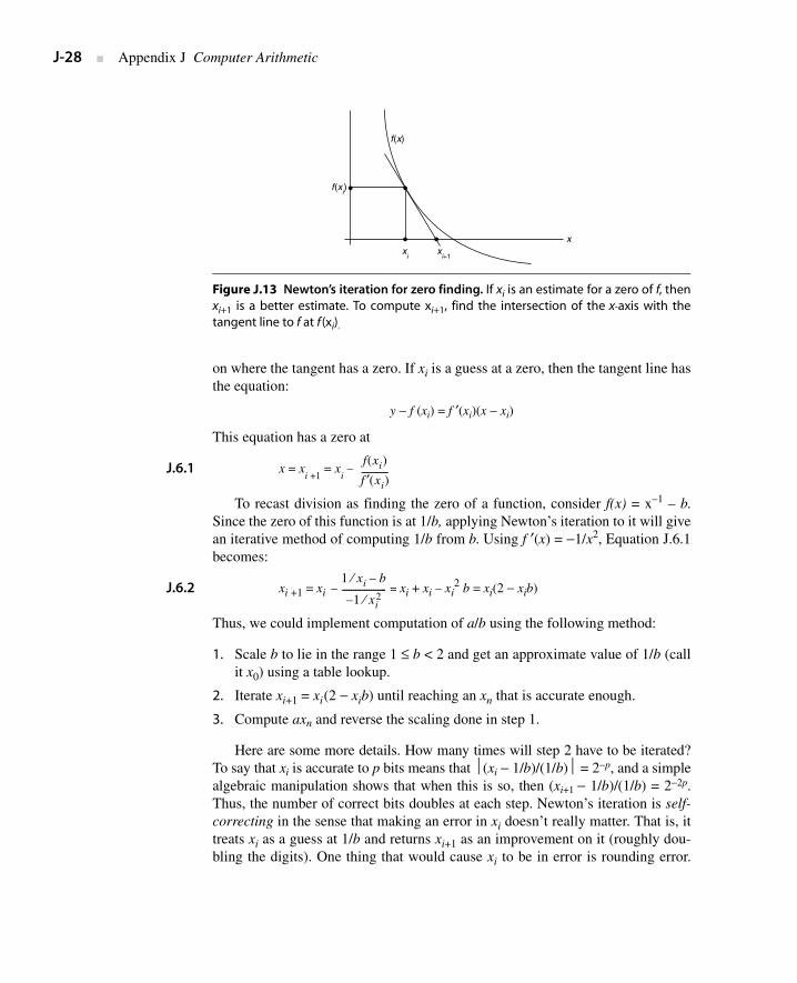
A different approach to division converges to the quotient at a quadraticrather than a linear rate. An actual machine that uses this algorithm will be dis-cussed in Section J.10. First, we will describe the two main iterative algorithms,and then we will discuss the pros and cons of iteration when compared with thedirect algorithms. A general technique for constructing iterative algorithms,called Newton’s iteration, is shown in Figure J.13. First, cast the problem in theform of finding the zero of a function. Then, starting from a guess for the zero,approximate the function by its tangent at that guess and form a new guess based
J.6 Division and Remainder
J-28 ■ Appendix J Computer Arithmetic
on where the tangent has a zero. If xi is a guess at a zero, then the tangent line hasthe equation:
y − f (xi) = f ′(xi)(x − xi)
This equation has a zero at
J.6.1 x = xi +1 = x
i −
To recast division as finding the zero of a function, consider f(x) = x–1 – b.Since the zero of this function is at 1/b, applying Newton’s iteration to it will givean iterative method of computing 1/b from b. Using f ′(x) = −1/x2, Equation J.6.1becomes:
J.6.2 xi +1 = xi − = xi + xi – xi
2 b = xi(2 − xib)
Thus, we could implement computation of a/b using the following method:
1. Scale b to lie in the range 1 ≤ b < 2 and get an approximate value of 1/b (callit x0) using a table lookup.
2. Iterate xi+1 = xi(2 − xib) until reaching an xn that is accurate enough.
3. Compute axn and reverse the scaling done in step 1.
Here are some more details. How many times will step 2 have to be iterated?To say that xi is accurate to p bits means that ⏐(xi − 1/b)/(1/b)⏐ = 2−p, and a simplealgebraic manipulation shows that when this is so, then (xi+1 − 1/b)/(1/b) = 2−2p.Thus, the number of correct bits doubles at each step. Newton’s iteration is self-correcting in the sense that making an error in xi doesn’t really matter. That is, ittreats xi as a guess at 1/b and returns xi+1 as an improvement on it (roughly dou-bling the digits). One thing that would cause xi to be in error is rounding error.
Figure J.13 Newton’s iteration for zero finding. If xi is an estimate for a zero of f, thenxi+1 is a better estimate. To compute xi+1, find the intersection of the x-axis with thetangent line to f at f (xi).
xx
i+1x
i
f(x)
f(xi)
f(xi)
f ′(xi)------------
1 xi⁄ b–
1 xi2⁄–
--------------------
J.6 Division and Remainder ■ J-29
More importantly, however, in the early iterations we can take advantage of thefact that we don’t expect many correct bits by performing the multiplication inreduced precision, thus gaining speed without sacrificing accuracy. Anotherapplication of Newton’s iteration is discussed in Exercise J.20.
The second iterative division method is sometimes called Goldschmidt’salgorithm. It is based on the idea that to compute a/b, you should multiply thenumerator and denominator by a number r with rb ≈ 1. In more detail, let x0 = aand y0þ= b. At each step compute xi+1 = rixi and yi+1 = riyi. Then the quotientxi+1/yi+1 = xi/yi = a/b is constant. If we pick ri so that yi → 1, then xi → a/b, sothe xi converge to the answer we want. This same idea can be used to computeother functions. For example, to compute the square root of a, let x0 = a and y0 =a, and at each step compute xi+1 = ri
2xi , yi+1 = riyi. Then xi+1/yi+12 = xi/yi
2 = 1/a,so if the ri are chosen to drive xi → 1, then yi → . This technique is used tocompute square roots on the TI 8847.
Returning to Goldschmidt’s division algorithm, set x0 = a and y0 = b, andwrite b = 1 − δ, where ⏐δ⏐ < 1. If we pick r0 = 1 + δ, then y1 = r0y0 = 1 − δ 2. Wenext pick r1 = 1 + δ2, so that y2 = r1y1 = 1 − δ 4, and so on. Since ⏐δ⏐ < 1, yi → 1.With this choice of ri, the xi will be computed as xi+1 = rixi = (1 + δ 2i)xi =(1 + (1 − b)2i)xi, or
J.6.3 xi+1
= a [1 + (1 − b)] [1 + (1 − b)2] [1 + (1 − b)4] ⋅⋅⋅ [1 + (1 − b)2 i ]
There appear to be two problems with this algorithm. First, convergence isslow when b is not near 1 (that is, δ is not near 0), and, second, the formula isn’tself-correcting—since the quotient is being computed as a product of independentterms, an error in one of them won’t get corrected. To deal with slow convergence,if you want to compute a/b, look up an approximate inverse to b (call it b′), andrun the algorithm on ab′/bb′. This will converge rapidly since bb′ ≈ 1.
To deal with the self-correction problem, the computation should be run witha few bits of extra precision to compensate for rounding errors. However, Gold-schmidt’s algorithm does have a weak form of self-correction, in that the precisevalue of the ri does not matter. Thus, in the first few iterations, when the fullprecision of 1 – δ 2i is not needed you can choose ri to be a truncation of 1 + δ 2i,which may make these iterations run faster without affecting the speed of conver-gence. If ri is truncated, then yi is no longer exactly 1 – δ 2i. Thus, Equation J.6.3can no longer be used, but it is easy to organize the computation so that it doesnot depend on the precise value of ri. With these changes, Goldschmidt’s algo-rithm is as follows (the notes in brackets show the connection with our earlierformulas).
1. Scale a and b so that 1 ≤ b < 2.
2. Look up an approximation to 1/b (call it b′) in a table.
3. Set x0 = ab′ and y0 = bb′.
a
J-30 ■ Appendix J Computer Arithmetic
4. Iterate until xi is close enough to a/b:
Loop
r ≈ 2 − y [if yi = 1 + δi, then r ≈ 1 − δi]
y = y × r [yi+1 = yi × r ≈ 1 − δi2]
xi+1 = xi × r [xi+1 = xi × r]
End loop
The two iteration methods are related. Suppose in Newton’s method that weunroll the iteration and compute each term xi+1 directly in terms of b, instead ofrecursively in terms of xi. By carrying out this calculation (see Exercise J.22), wediscover that
xi+1 = x0(2 − x0b) [(1 + (x0b − 1)2] [1 + (x0b − 1)4] … [1 + (x0b − 1)2i]
This formula is very similar to Equation J.6.3. In fact, they are identical if a and bin J.6.3 are replaced with ax0, bx0, and a = 1. Thus, if the iterations were done toinfinite precision, the two methods would yield exactly the same sequence xi.
The advantage of iteration is that it doesn’t require special divide hardware.Instead, it can use the multiplier (which, however, requires extra control). Fur-ther, on each step, it delivers twice as many digits as in the previous step—unlikeordinary division, which produces a fixed number of digits at every step.
There are two disadvantages with inverting by iteration. The first is that theIEEE standard requires division to be correctly rounded, but iteration only deliv-ers a result that is close to the correctly rounded answer. In the case of Newton’siteration, which computes 1/b instead of a/b directly, there is an additionalproblem. Even if 1/b were correctly rounded, there is no guarantee that a/b willbe. An example in decimal with p = 2 is a = 13, b = 51. Then a/b = .2549. . . ,which rounds to .25. But 1/b = .0196. . . , which rounds to .020, and then a × .020= .26, which is off by 1. The second disadvantage is that iteration does not give aremainder. This is especially troublesome if the floating-point divide hardware isbeing used to perform integer division, since a remainder operation is present inalmost every high-level language.
Traditional folklore has held that the way to get a correctly rounded resultfrom iteration is to compute 1/b to slightly more than 2p bits, compute a/b toslightly more than 2p bits, and then round to p bits. However, there is a faster way,which apparently was first implemented on the TI 8847. In this method, a/b iscomputed to about 6 extra bits of precision, giving a preliminary quotient q. Bycomparing qb with a (again with only 6 extra bits), it is possible to quickly decidewhether q is correctly rounded or whether it needs to be bumped up or down by 1in the least-significant place. This algorithm is explored further in Exercise J.21.
One factor to take into account when deciding on division algorithms is therelative speed of division and multiplication. Since division is more complexthan multiplication, it will run more slowly. A common rule of thumb is thatdivision algorithms should try to achieve a speed that is about one-third that of
J.6 Division and Remainder ■ J-31
multiplication. One argument in favor of this rule is that there are real pro-grams (such as some versions of spice) where the ratio of division to multi-plication is 1:3. Another place where a factor of 3 arises is in the standarditerative method for computing square root. This method involves one divisionper iteration, but it can be replaced by one using three multiplications. This isdiscussed in Exercise J.20.
Floating-Point Remainder
For nonnegative integers, integer division and remainder satisfy:
a = (a DIV b)b + a REM b, 0 ≤ a REM b < b
A floating-point remainder x REM y can be similarly defined as x = INT(x/y)y + xREM y. How should x/y be converted to an integer? The IEEE remainder functionuses the round-to-even rule. That is, pick n = INT (x/y) so that ⏐x/y − n⏐ ≤ 1/2.If two different n satisfy this relation, pick the even one. Then REM is definedto be x − yn. Unlike integers where 0 ≤ a REM b < b, for floating-point numbers
⏐x REM y⏐ ≤ y/2. Although this defines REM precisely, it is not a practical opera-tional definition, because n can be huge. In single precision, n could be as large as2127/2–126 = 2253 ≈ 1076.
There is a natural way to compute REM if a direct division algorithm is used.Proceed as if you were computing x/y. If x = s12e1 and y = s22e2 and the divider isas in Figure J.2(b) (page J-4), then load s1 into P and s2 into B. After e1 − e2division steps, the P register will hold a number r of the form x − yn satisfying0 ≤ r < y. Since the IEEE remainder satisfies ⏐REM⏐ ≤ y/2, REM is equal to eitherr or r − y. It is only necessary to keep track of the last quotient bit produced,which is needed to resolve halfway cases. Unfortunately, e1 − e2 can be a lot ofsteps, and floating-point units typically have a maximum amount of time they areallowed to spend on one instruction. Thus, it is usually not possible to implementREM directly. None of the chips discussed in Section J.10 implements REM, butthey could by providing a remainder-step instruction—this is what is done on theIntel 8087 family. A remainder step takes as arguments two numbers x and y, andperforms divide steps until either the remainder is in P or n steps have been per-formed, where n is a small number, such as the number of steps required for divi-sion in the highest-supported precision. Then REM can be implemented as asoftware routine that calls the REM step instruction ⎣(e1 − e2)/n⎦ times, initiallyusing x as the numerator but then replacing it with the remainder from the previ-ous REM step.
REM can be used for computing trigonometric functions. To simplify things,imagine that we are working in base 10 with five significant figures, and considercomputing sin x. Suppose that x = 7. Then we can reduce by π = 3.1416 and com-pute sin(7) = sin(7 − 2 × 3.1416) = sin(0.7168) instead. But, suppose we want tocompute sin(2.0 × 10⁵). Then 2 × 10⁵/3.1416 = 63661.8, which in our five-placesystem comes out to be 63662. Since multiplying 3.1416 times 63662 gives200000.5392, which rounds to 2.0000 × 10⁵, argument reduction reduces 2 × 10⁵
to 0, which is not even close to being correct. The problem is that our five-place
J-32 ■ Appendix J Computer Arithmetic
system does not have the precision to do correct argument reduction. Suppose wehad the REM operator. Then we could compute 2 × 10⁵ REM 3.1416 and get −.53920.However, this is still not correct because we used 3.1416, which is an approximationfor π. The value of 2 × 10⁵ REM π is −.071513.
Traditionally, there have been two approaches to computing periodic func-tions with large arguments. The first is to return an error for their value when x islarge. The second is to store π to a very large number of places and do exact argu-ment reduction. The REM operator is not much help in either of these situations.There is a third approach that has been used in some math libraries, such as theBerkeley UNIX 4.3bsd release. In these libraries, π is computed to the nearestfloating-point number. Let’s call this machine π, and denote it by π′. Then, whencomputing sin x, reduce x using x REM π′. As we saw in the above example, xREM π ′ is quite different from x REM π when x is large, so that computing sin x assin(x REM π ′) will not give the exact value of sin x. However, computing trigono-metric functions in this fashion has the property that all familiar identities (suchas sin2 x + cos2 x = 1) are true to within a few rounding errors. Thus, using REM
together with machine π provides a simple method of computing trigonometricfunctions that is accurate for small arguments and still may be useful for largearguments.
When REM is used for argument reduction, it is very handy if it also returnsthe low-order bits of n (where x REM y = x − ny). This is because a practicalimplementation of trigonometric functions will reduce by something smallerthan 2π. For example, it might use π/2, exploiting identities such as sin(x − π/2)= –cos x, sin(x − π) = −sin x. Then the low bits of n are needed to choose thecorrect identity.
Before leaving the subject of floating-point arithmetic, we present a few addi-tional topics.
Fused Multiply-Add
Probably the most common use of floating-point units is performing matrix oper-ations, and the most frequent matrix operation is multiplying a matrix times amatrix (or vector), which boils down to computing an inner product, x1⋅y1 + x2⋅y2+ . . . + xn⋅yn. Computing this requires a series of multiply-add combinations.
Motivated by this, the IBM RS/6000 introduced a single instruction that com-putes ab + c, the fused multiply-add. Although this requires being able to readthree operands in a single instruction, it has the potential for improving the per-formance of computing inner products.
The fused multiply-add computes ab + c exactly and then rounds. Althoughrounding only once increases the accuracy of inner products somewhat, that isnot its primary motivation. There are two main advantages of rounding once.
J.7 More on Floating-Point Arithmetic
J.7 More on Floating-Point Arithmetic ■ J-33
First, as we saw in the previous sections, rounding is expensive to implementbecause it may require an addition. By rounding only once, an addition operationhas been eliminated. Second, the extra accuracy of fused multiply-add can beused to compute correctly rounded division and square root when these are notavailable directly in hardware. Fused multiply-add can also be used to implementefficient floating-point multiple-precision packages.
The implementation of correctly rounded division using fused multiply-addhas many details, but the main idea is simple. Consider again the example fromSection J.6 (page J-30), which was computing a/b with a = 13, b = 51. Then 1/brounds to b′ = .020, and ab′ rounds to q′ = .26, which is not the correctly roundedquotient. Applying fused multiply-add twice will correctly adjust the result, viathe formulas
r = a − bq′
q′′ = q′ + rb′
Computing to two-digit accuracy, bq′ = 51 × .26 rounds to 13, and so r = a − bq′would be 0, giving no adjustment. But using fused multiply-add gives r = a − bq′= 13 − (51 × .26) = −.26, and then q′′ = q′ + rb′ = .26 − .0052 = .2548, whichrounds to the correct quotient, .25. More details can be found in the papers byMontoye, Hokenek, and Runyon [1990] and Markstein [1990].
Precisions
The standard specifies four precisions: single, single extended, double, and dou-ble extended. The properties of these precisions are summarized in Figure J.7(page J-16). Implementations are not required to have all four precisions, but areencouraged to support either the combination of single and single extended or allof single, double, and double extended. Because of the widespread use of doubleprecision in scientific computing, double precision is almost always imple-mented. Thus, the computer designer usually only has to decide whether to sup-port double extended and, if so, how many bits it should have.
The Motorola 68882 and Intel 387 coprocessors implement extended preci-sion using the smallest allowable size of 80 bits (64 bits of significand). However,many of the more recently designed, high-performance floating-point chips donot implement 80-bit extended precision. One reason is that the 80-bit width ofextended precision is awkward for 64-bit buses and registers. Some new architec-tures, such as SPARC V8 and PA-RISC, specify a 128-bit extended (or quad)precision. They have established a de facto convention for quad that has 15 bits ofexponent and 113 bits of significand.
Although most high-level languages do not provide access to extended pre-cision, it is very useful to writers of mathematical software. As an example,consider writing a library routine to compute the length of a vector (x,y) inthe plane, namely, . If x is larger than 2Emax/2, then computing this inthe obvious way will overflow. This means that either the allowable exponent
x2 y2+
J-34 ■ Appendix J Computer Arithmetic
range for this subroutine will be cut in half or a more complex algorithm usingscaling will have to be employed. But, if extended precision is available, thenthe simple algorithm will work. Computing the length of a vector is a simpletask, and it is not difficult to come up with an algorithm that doesn’t overflow.However, there are more complex problems for which extended precisionmeans the difference between a simple, fast algorithm and a much more com-plex one. One of the best examples of this is binary-to-decimal conversion. Anefficient algorithm for binary-to-decimal conversion that makes essential use ofextended precision is very readably presented in Coonen [1984]. This algo-rithm is also briefly sketched in Goldberg [1991]. Computing accurate valuesfor transcendental functions is another example of a problem that is made mucheasier if extended precision is present.
One very important fact about precision concerns double rounding. To illus-trate in decimals, suppose that we want to compute 1.9 × 0.66 and that single pre-cision is two digits, while extended precision is three digits. The exact result ofthe product is 1.254. Rounded to extended precision, the result is 1.25. When fur-ther rounded to single precision, we get 1.2. However, the result of 1.9 × 0.66 cor-rectly rounded to single precision is 1.3. Thus, rounding twice may not producethe same result as rounding once. Suppose you want to build hardware that onlydoes double-precision arithmetic. Can you simulate single precision by comput-ing first in double precision and then rounding to single? The above example sug-gests that you can’t. However, double rounding is not always dangerous. In fact,the following rule is true (this is not easy to prove, but see Exercise J.25).
If x and y have p-bit significands, and x + y is computed exactly and then roundedto q places, a second rounding to p places will not change the answer if q ≥ 2p + 2.This is true not only for addition, but also for multiplication, division, and squareroot.
In our example above, q = 3 and p = 2, so q Š 2p + 2 is not true. On the otherhand, for IEEE arithmetic, double precision has q = 53 and p = 24, so q = 53 Š 2p+ 2 = 50. Thus, single precision can be implemented by computing in double preci-sion—that is, computing the answer exactly and then rounding to double—andthen rounding to single precision.
Exceptions
The IEEE standard defines five exceptions: underflow, overflow, divide by zero,inexact, and invalid. By default, when these exceptions occur, they merely set aflag and the computation continues. The flags are sticky, meaning that once setthey remain set until explicitly cleared. The standard strongly encourages imple-mentations to provide a trap-enable bit for each exception. When an exceptionwith an enabled trap handler occurs, a user trap handler is called, and the value ofthe associated exception flag is undefined. In Section J.3 we mentioned that has the value NaN and 1/0 is ∞. These are examples of operations that raise anexception. By default, computing sets the invalid flag and returns the valueNaN. Similarly 1/0 sets the divide-by-zero flag and returns ∞.
3–
3–
J.7 More on Floating-Point Arithmetic ■ J-35
The underflow, overflow, and divide-by-zero exceptions are found in mostother systems. The invalid exception is for the result of operations such as ,0/0, or ∞ − ∞, which don’t have any natural value as a floating-point number oras ±∞. The inexact exception is peculiar to IEEE arithmetic and occurs eitherwhen the result of an operation must be rounded or when it overflows. In fact,since 1/0 and an operation that overflows both deliver ∞, the exception flags mustbe consulted to distinguish between them. The inexact exception is an unusual“exception,” in that it is not really an exceptional condition because it occurs sofrequently. Thus, enabling a trap handler for the inexact exception will mostlikely have a severe impact on performance. Enabling a trap handler doesn’taffect whether an operation is exceptional except in the case of underflow. This isdiscussed below.
The IEEE standard assumes that when a trap occurs, it is possible to identifythe operation that trapped and its operands. On machines with pipelining or mul-tiple arithmetic units, when an exception occurs, it may not be enough to simplyhave the trap handler examine the program counter. Hardware support may benecessary to identify exactly which operation trapped.
Another problem is illustrated by the following program fragment.
r1 = r2/r3r2 = r4 + r5
These two instructions might well be executed in parallel. If the divide traps, itsargument r2 could already have been overwritten by the addition, especiallysince addition is almost always faster than division. Computer systems that sup-port trapping in the IEEE standard must provide some way to save the value ofr2, either in hardware or by having the compiler avoid such a situation in the firstplace. This kind of problem is not peculiar to floating point. In the sequence
r1 = 0(r2)r2 = r3
it would be efficient to execute r2 = r3 while waiting for memory. But, if access-ing 0(r2) causes a page fault, r2 might no longer be available for restarting theinstruction r1 = 0(r2).
One approach to this problem, used in the MIPS R3010, is to identifyinstructions that may cause an exception early in the instruction cycle. For exam-ple, an addition can overflow only if one of the operands has an exponent ofEmax, and so on. This early check is conservative: It might flag an operation thatdoesn’t actually cause an exception. However, if such false positives are rare,then this technique will have excellent performance. When an instruction istagged as being possibly exceptional, special code in a trap handler can computeit without destroying any state. Remember that all these problems occur onlywhen trap handlers are enabled. Otherwise, setting the exception flags duringnormal processing is straightforward.
1–
J-36 ■ Appendix J Computer Arithmetic
Underflow
We have alluded several times to the fact that detection of underflow is morecomplex than for the other exceptions. The IEEE standard specifies that if anunderflow trap handler is enabled, the system must trap if the result is denormal.On the other hand, if trap handlers are disabled, then the underflow flag is setonly if there is a loss of accuracy—that is, if the result must be rounded. Therationale is, if no accuracy is lost on an underflow, there is no point in setting awarning flag. But if a trap handler is enabled, the user might be trying to simulateflush-to-zero and should therefore be notified whenever a result dips below 1.0 ×2Emin.
So if there is no trap handler, the underflow exception is signaled only whenthe result is denormal and inexact, but the definitions of denormal and inexact areboth subject to multiple interpretations. Normally, inexact means there was aresult that couldn’t be represented exactly and had to be rounded. Consider theexample (in a base 2 floating-point system with 3-bit significands) of (1.112 × 2−2)× (1.112 × 2Emin) = 0.1100012 × 2Emin, with round to nearest in effect. The deliv-ered result is 0.112 × 2Emin, which had to be rounded, causing inexact to be sig-naled. But is it correct to also signal underflow? Gradual underflow losessignificance because the exponent range is bounded. If the exponent range wereunbounded, the delivered result would be 1.102 × 2Emin–1, exactly the sameanswer obtained with gradual underflow. The fact that denormalized numbershave fewer bits in their significand than normalized numbers therefore doesn’tmake any difference in this case. The commentary to the standard [Cody et al.1984] encourages this as the criterion for setting the underflow flag. That is, itshould be set whenever the delivered result is different from what would be deliv-ered in a system with the same fraction size, but with a very large exponent range.However, owing to the difficulty of implementing this scheme, the standardallows setting the underflow flag whenever the result is denormal and differentfrom the infinitely precise result.
There are two possible definitions of what it means for a result to be denor-mal. Consider the example of 1.102 × 2–1 multiplied by 1.012 × 2Emin. The exactproduct is 0.1111 × 2Emin. The rounded result is the normal number 1.002 × 2Emin.Should underflow be signaled? Signaling underflow means that you are using thebefore rounding rule, because the result was denormal before rounding. Not sig-naling underflow means that you are using the after rounding rule, because theresult is normalized after rounding. The IEEE standard provides for choosingeither rule; however, the one chosen must be used consistently for all operations.
To illustrate these rules, consider floating-point addition. When the result ofan addition (or subtraction) is denormal, it is always exact. Thus, the underflowflag never needs to be set for addition. That’s because if traps are not enabledthen no exception is raised. And if traps are enabled, the value of the underflowflag is undefined, so again it doesn’t need to be set.
One final subtlety should be mentioned concerning underflow. When there isno underflow trap handler, the result of an operation on p-bit numbers that causes
J.8 Speeding Up Integer Addition ■ J-37
an underflow is a denormal number with p − 1 or fewer bits of precision. Whentraps are enabled, the trap handler is provided with the result of the operationrounded to p bits and with the exponent wrapped around. Now there is a potentialdouble-rounding problem. If the trap handler wants to return the denormal result,it can’t just round its argument, because that might lead to a double-roundingerror. Thus, the trap handler must be passed at least one extra bit of information ifit is to be able to deliver the correctly rounded result.
The previous section showed that many steps go into implementing floating-pointoperations; however, each floating-point operation eventually reduces to an inte-ger operation. Thus, increasing the speed of integer operations will also lead tofaster floating point.
Integer addition is the simplest operation and the most important. Even forprograms that don’t do explicit arithmetic, addition must be performed to incre-ment the program counter and to calculate addresses. Despite the simplicity ofaddition, there isn’t a single best way to perform high-speed addition. We willdiscuss three techniques that are in current use: carry-lookahead, carry-skip, andcarry-select.
Carry-Lookahead
An n-bit adder is just a combinational circuit. It can therefore be written by alogic formula whose form is a sum of products and can be computed by a circuitwith two levels of logic. How do you figure out what this circuit looks like? FromEquation J.2.1 (page J-3) the formula for the ith sum can be written as:
J.8.1 si = ai bi ci + ai bi ci + ai bi ci + ai bi ci
where ci is both the carry-in to the ith adder and the carry-out from the (i−1)-stadder.
The problem with this formula is that, although we know the values of ai andbi—they are inputs to the circuit—we don’t know ci. So our goal is to write ci interms of ai and bi. To accomplish this, we first rewrite Equation J.2.2 (page J-3)as:
J.8.2 ci = gi –1+ p i –1c i –1, g i –1 = a i –1b i –1, p i –1 = a i –1 + b i –1
Here is the reason for the symbols p and g: If gi–1 is true, then ci is certainlytrue, so a carry is generated. Thus, g is for generate. If pi–1 is true, then if ci–1 istrue, it is propagated to ci. Start with Equation J.8.1 and use Equation J.8.2 toreplace ci with gi–1 + pi–1ci–1. Then, use Equation J.8.2 with i− 1 in place of i toreplace ci–1 with ci–2, and so on. This gives the result:
J.8.3 ci = gi–1 + pi–1 gi–2 + pi–1 pi–2 gi–3 + ⋅ ⋅ ⋅ + pi–1 pi–2 ⋅ ⋅ ⋅ p1 g0 + pi–1 pi–2 ⋅ ⋅ ⋅ p1p0c0
J.8 Speeding Up Integer Addition
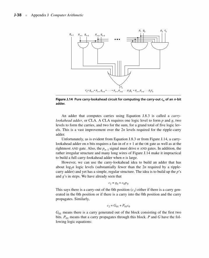
J-38 ■ Appendix J Computer Arithmetic
An adder that computes carries using Equation J.8.3 is called a carry-lookahead adder, or CLA. A CLA requires one logic level to form p and g, twolevels to form the carries, and two for the sum, for a grand total of five logic lev-els. This is a vast improvement over the 2n levels required for the ripple-carryadder.
Unfortunately, as is evident from Equation J.8.3 or from Figure J.14, a carry-lookahead adder on n bits requires a fan-in of n + 1 at the OR gate as well as at therightmost AND gate. Also, the pn–1 signal must drive n AND gates. In addition, therather irregular structure and many long wires of Figure J.14 make it impracticalto build a full carry-lookahead adder when n is large.
However, we can use the carry-lookahead idea to build an adder that hasabout log2n logic levels (substantially fewer than the 2n required by a ripple-carry adder) and yet has a simple, regular structure. The idea is to build up the p’sand g’s in steps. We have already seen that
c1 = g0 + c0p0
This says there is a carry-out of the 0th position (c1) either if there is a carry gen-erated in the 0th position or if there is a carry into the 0th position and the carrypropagates. Similarly,
c2 = G01 + P01c0
G01 means there is a carry generated out of the block consisting of the first twobits. P01 means that a carry propagates through this block. P and G have the fol-lowing logic equations:
Figure J.14 Pure carry-lookahead circuit for computing the carry-out cn of an n-bitadder.
gn–1 p
n–1
cn
gn–2
pn–2
gn–3
p1
g0
p0
c0
cn= g
n–1+ p
n–1 g
n–2 + . . . + p
n–1 p
n–2 . . . p
1g
0 + p
n–1 p
n–2 . . . p
0c
0
J.8 Speeding Up Integer Addition ■ J-39
G01 = g1 + p1g0
P01 = p1p0
More generally, for any j with i < j, j + 1 < k, we have the recursive relations:
J.8.4 ck+1 = Gik + Pikci
J.8.5 Gik = Gj+1,k + Pj+1,kGij
J.8.6 Pik = Pij Pj+1,k
Equation J.8.5 says that a carry is generated out of the block consisting of bits ithrough k inclusive if it is generated in the high-order part of the block (j + 1, k)or if it is generated in the low-order part of the block (i,j) and then propagatedthrough the high part. These equations will also hold for i ≤ j < k if we set Gii = giand Pii = pi.
Example Express P03 and G03 in terms of p’s and g’s.
Answer Using Equation J.8.6, P03 = P01P23 = P00P11P22P33. Since Pii = pi, P03 =p0p1p2p3. For G03, Equation J.8.5 says G03 = G23 + P23G01 = (G33 + P33G22) +(P22P33)(G11 + P11G00) = g3 + p3g2 + p3 p2 g1 + p3 p2 p1g0.
With these preliminaries out of the way, we can now show the design of apractical CLA. The adder consists of two parts. The first part computes variousvalues of P and G from pi and gi, using Equations J.8.5 and J.8.6; the second partuses these P and G values to compute all the carries via Equation J.8.4. The firstpart of the design is shown in Figure J.15. At the top of the diagram, input num-bers a7. . . a0 and b7. . . b0 are converted to p’s and g’s using cells of type 1. Thenvarious P’s and G’s are generated by combining cells of type 2 in a binary treestructure. The second part of the design is shown in Figure J.16. By feeding c0 inat the bottom of this tree, all the carry bits come out at the top. Each cell mustknow a pair of (P,G) values in order to do the conversion, and the value it needsis written inside the cells. Now compare Figures J.15 and J.16. There is a one-to-one correspondence between cells, and the value of (P,G) needed by thecarry-generating cells is exactly the value known by the corresponding (P,G)-generating cells. The combined cell is shown in Figure J.17. The numbers to beadded flow into the top and downward through the tree, combining with c0 at thebottom and flowing back up the tree to form the carries. Note that one thing ismissing from Figure J.17: a small piece of extra logic to compute c8 for thecarry-out of the adder.
The bits in a CLA must pass through about log2 n logic levels, compared with2n for a ripple-carry adder. This is a substantial speed improvement, especiallyfor a large n. Whereas the ripple-carry adder had n cells, however, the CLA has
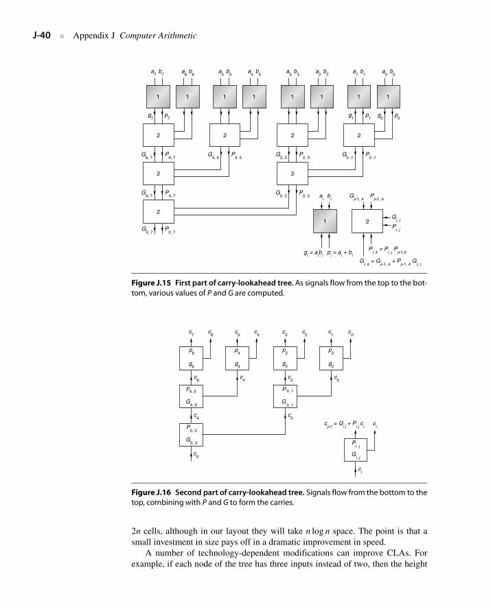
J-40 ■ Appendix J Computer Arithmetic
2n cells, although in our layout they will take n log n space. The point is that asmall investment in size pays off in a dramatic improvement in speed.
A number of technology-dependent modifications can improve CLAs. Forexample, if each node of the tree has three inputs instead of two, then the height
Figure J.15 First part of carry-lookahead tree. As signals flow from the top to the bot-tom, various values of P and G are computed.
Figure J.16 Second part of carry-lookahead tree. Signals flow from the bottom to thetop, combining with P and G to form the carries.
1 1 1 1 1 1
1
1 1
2
2
2
2
2
a7
b7
a6
b6
a5
b5
a4
b4
a3
b3
a2
b2
a1
b1
a0
b0
p0
g0
p1
g1
g7
p7
G6, 7
P6, 7
G4, 5
P4, 5
G2, 3
P2, 3
G0 ,1
P0 ,1
G4, 7
P4, 7
G0, 3
P0, 3
G0, 7
P0, 7
gi = a
ib
i p
i = a
i + b
i G
i, k = G
j+1, k + P
j+1, k G
i, j
Pi, k
= Pi, j
Pj+1,k
Pi, j
Gi, j
Gj+1, k
ai
bi
Pj+1, k
2 2
2
c7
c6
c5
c4
c3
c2
c1
c0
p0
g0
p2
g2
P 0, 1
G0, 1
p4
g4
p6
g6
c6
c4
c2
c0
c0
c4
c0
cj+1
= Gi j
+ Pi j
ci
ci
Pi, j
Gi, j
ci
p4, 5
G4, 5
P0, 3
G0, 3
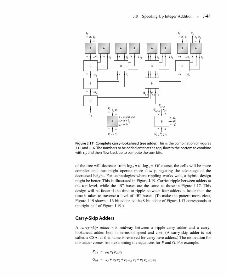
J.8 Speeding Up Integer Addition ■ J-41
of the tree will decrease from log2 n to log3 n. Of course, the cells will be morecomplex and thus might operate more slowly, negating the advantage of thedecreased height. For technologies where rippling works well, a hybrid designmight be better. This is illustrated in Figure J.19. Carries ripple between adders atthe top level, while the “B” boxes are the same as those in Figure J.17. Thisdesign will be faster if the time to ripple between four adders is faster than thetime it takes to traverse a level of “B” boxes. (To make the pattern more clear,Figure J.19 shows a 16-bit adder, so the 8-bit adder of Figure J.17 corresponds tothe right half of Figure J.19.)
Carry-Skip Adders
A carry-skip adder sits midway between a ripple-carry adder and a carry-lookahead adder, both in terms of speed and cost. (A carry-skip adder is notcalled a CSA, as that name is reserved for carry-save adders.) The motivation forthis adder comes from examining the equations for P and G. For example,
P03 = p0 p1 p2 p3
G03 = g3 + p3 g2 + p3 p2 g1 + p3 p2 p1 g0
Figure J.17 Complete carry-lookahead tree adder. This is the combination of FiguresJ.15 and J.16. The numbers to be added enter at the top, flow to the bottom to combinewith c0, and then flow back up to compute the sum bits.
A A
A
B
B
s7
a7
b7
c7
A A A A A A
B
B B B
+ +
B
s1
a1
b1
s0
a0
b0
c6 c
5c
4c
3c
2c
1c
0
c0
c0
P0, 3
G0, 3
c4
c0
si a
ib
i
si = a
i p
i = a
i + b
ig
i = a
i b
i
gi
pi
ci G
i, kP
i, kc
i
ci
Pi j
Gij
cj +1
Pj +1,k
Gj +1,k
bi
ci
c2
c4c
6
B
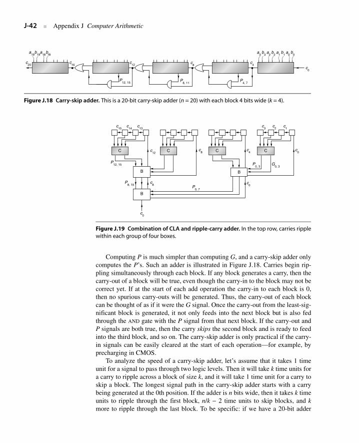
J-42 ■ Appendix J Computer Arithmetic
Computing P is much simpler than computing G, and a carry-skip adder onlycomputes the P’s. Such an adder is illustrated in Figure J.18. Carries begin rip-pling simultaneously through each block. If any block generates a carry, then thecarry-out of a block will be true, even though the carry-in to the block may not becorrect yet. If at the start of each add operation the carry-in to each block is 0,then no spurious carry-outs will be generated. Thus, the carry-out of each blockcan be thought of as if it were the G signal. Once the carry-out from the least-sig-nificant block is generated, it not only feeds into the next block but is also fedthrough the AND gate with the P signal from that next block. If the carry-out andP signals are both true, then the carry skips the second block and is ready to feedinto the third block, and so on. The carry-skip adder is only practical if the carry-in signals can be easily cleared at the start of each operation—for example, byprecharging in CMOS.
To analyze the speed of a carry-skip adder, let’s assume that it takes 1 timeunit for a signal to pass through two logic levels. Then it will take k time units fora carry to ripple across a block of size k, and it will take 1 time unit for a carry toskip a block. The longest signal path in the carry-skip adder starts with a carrybeing generated at the 0th position. If the adder is n bits wide, then it takes k timeunits to ripple through the first block, n/k − 2 time units to skip blocks, and kmore to ripple through the last block. To be specific: if we have a 20-bit adder
Figure J.18 Carry-skip adder. This is a 20-bit carry-skip adder (n = 20) with each block 4 bits wide (k = 4).
Figure J.19 Combination of CLA and ripple-carry adder. In the top row, carries ripplewithin each group of four boxes.
a3
b3
a2
b2
a1
b1
a0
b0
c4
c0
P4, 7
c8
c12
P12, 15 P
8, 11
a19
a18
b19
b18
c16
c20
c15
c14
c13
c12
P12, 15
P8, 15
c8
c0
P0, 7
c8
c4
c0
c0
G0, 3
P0, 3
c1
c2
c3
C
B
B
C C C
B
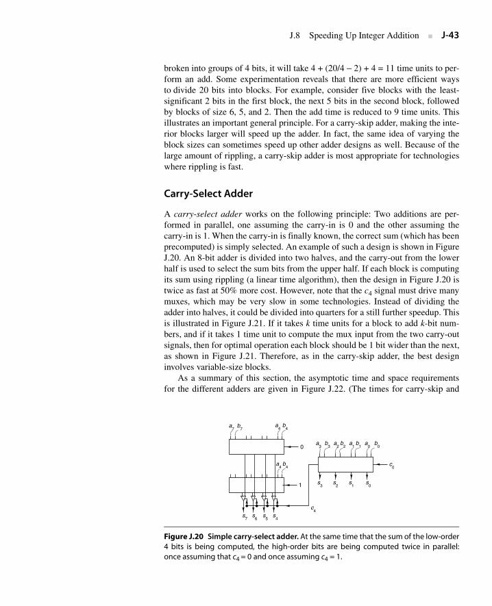
J.8 Speeding Up Integer Addition ■ J-43
broken into groups of 4 bits, it will take 4 + (20/4 − 2) + 4 = 11 time units to per-form an add. Some experimentation reveals that there are more efficient waysto divide 20 bits into blocks. For example, consider five blocks with the least-significant 2 bits in the first block, the next 5 bits in the second block, followedby blocks of size 6, 5, and 2. Then the add time is reduced to 9 time units. Thisillustrates an important general principle. For a carry-skip adder, making the inte-rior blocks larger will speed up the adder. In fact, the same idea of varying theblock sizes can sometimes speed up other adder designs as well. Because of thelarge amount of rippling, a carry-skip adder is most appropriate for technologieswhere rippling is fast.
Carry-Select Adder
A carry-select adder works on the following principle: Two additions are per-formed in parallel, one assuming the carry-in is 0 and the other assuming thecarry-in is 1. When the carry-in is finally known, the correct sum (which has beenprecomputed) is simply selected. An example of such a design is shown in FigureJ.20. An 8-bit adder is divided into two halves, and the carry-out from the lowerhalf is used to select the sum bits from the upper half. If each block is computingits sum using rippling (a linear time algorithm), then the design in Figure J.20 istwice as fast at 50% more cost. However, note that the c4 signal must drive manymuxes, which may be very slow in some technologies. Instead of dividing theadder into halves, it could be divided into quarters for a still further speedup. Thisis illustrated in Figure J.21. If it takes k time units for a block to add k-bit num-bers, and if it takes 1 time unit to compute the mux input from the two carry-outsignals, then for optimal operation each block should be 1 bit wider than the next,as shown in Figure J.21. Therefore, as in the carry-skip adder, the best designinvolves variable-size blocks.
As a summary of this section, the asymptotic time and space requirementsfor the different adders are given in Figure J.22. (The times for carry-skip and
Figure J.20 Simple carry-select adder. At the same time that the sum of the low-order4 bits is being computed, the high-order bits are being computed twice in parallel:once assuming that c4 = 0 and once assuming c4 = 1.
c0
s0
s1
s2
s3
c4
s4
a4
b4
s5
s6
s7
1
0a
3 b
3 a
2 b
2 a
1 b
1 a
0 b
0
a7 b
7a
4 b
4
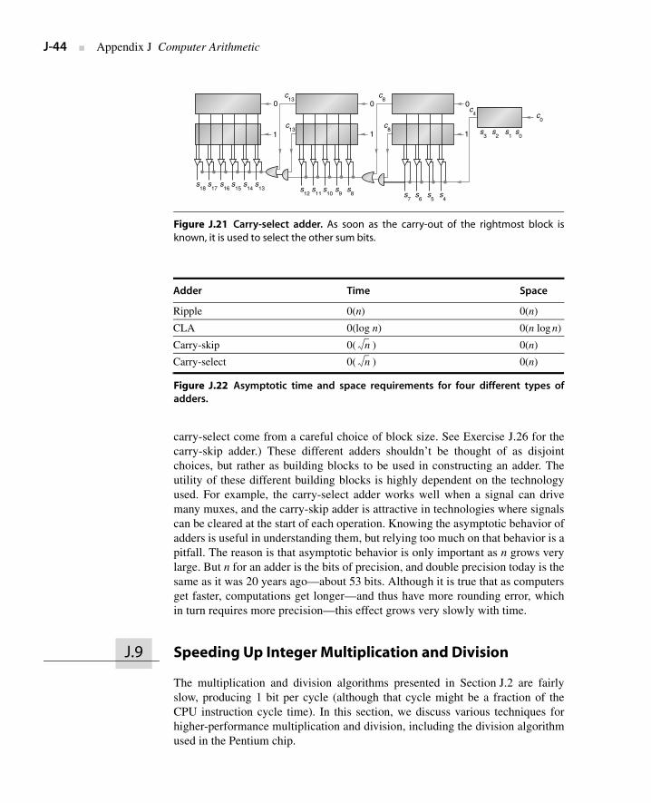
J-44 ■ Appendix J Computer Arithmetic
carry-select come from a careful choice of block size. See Exercise J.26 for thecarry-skip adder.) These different adders shouldn’t be thought of as disjointchoices, but rather as building blocks to be used in constructing an adder. Theutility of these different building blocks is highly dependent on the technologyused. For example, the carry-select adder works well when a signal can drivemany muxes, and the carry-skip adder is attractive in technologies where signalscan be cleared at the start of each operation. Knowing the asymptotic behavior ofadders is useful in understanding them, but relying too much on that behavior is apitfall. The reason is that asymptotic behavior is only important as n grows verylarge. But n for an adder is the bits of precision, and double precision today is thesame as it was 20 years ago—about 53 bits. Although it is true that as computersget faster, computations get longer—and thus have more rounding error, whichin turn requires more precision—this effect grows very slowly with time.
The multiplication and division algorithms presented in Section J.2 are fairlyslow, producing 1 bit per cycle (although that cycle might be a fraction of theCPU instruction cycle time). In this section, we discuss various techniques forhigher-performance multiplication and division, including the division algorithmused in the Pentium chip.
Figure J.21 Carry-select adder. As soon as the carry-out of the rightmost block isknown, it is used to select the other sum bits.
Adder Time Space
Ripple 0(n) 0(n)
CLA 0(log n) 0(n log n)
Carry-skip 0( ) 0(n)
Carry-select 0( ) 0(n)
Figure J.22 Asymptotic time and space requirements for four different types ofadders.
c13
c8
c4 c
0
s0
s1
s2
s3
s4
s5
s6
s7
s8
s9
1
00
1
s10
s11
s12
s13
c13
c8
1
s14
s15
s16
s17
s18
0
n
n
J.9 Speeding Up Integer Multiplication and Division
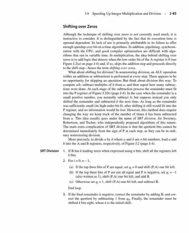
J.9 Speeding Up Integer Multiplication and Division ■ J-45
Shifting over Zeros
Although the technique of shifting over zeros is not currently used much, it isinstructive to consider. It is distinguished by the fact that its execution time isoperand dependent. Its lack of use is primarily attributable to its failure to offerenough speedup over bit-at-a-time algorithms. In addition, pipelining, synchroni-zation with the CPU, and good compiler optimization are difficult with algo-rithms that run in variable time. In multiplication, the idea behind shifting overzeros is to add logic that detects when the low-order bit of the A register is 0 (seeFigure J.2(a) on page J-4) and, if so, skips the addition step and proceeds directlyto the shift step—hence the term shifting over zeros.
What about shifting for division? In nonrestoring division, an ALU operation(either an addition or subtraction) is performed at every step. There appears to beno opportunity for skipping an operation. But think about division this way: Tocompute a/b, subtract multiples of b from a, and then report how many subtrac-tions were done. At each stage of the subtraction process the remainder must fitinto the P register of Figure J.2(b) (page J-4). In the case when the remainder is asmall positive number, you normally subtract b; but suppose instead you onlyshifted the remainder and subtracted b the next time. As long as the remainderwas sufficiently small (its high-order bit 0), after shifting it still would fit into theP register, and no information would be lost. However, this method does requirechanging the way we keep track of the number of times b has been subtractedfrom a. This idea usually goes under the name of SRT division, for Sweeney,Robertson, and Tocher, who independently proposed algorithms of this nature.The main extra complication of SRT division is that the quotient bits cannot bedetermined immediately from the sign of P at each step, as they can be in ordi-nary nonrestoring division.
More precisely, to divide a by b where a and b are n-bit numbers, load a andb into the A and B registers, respectively, of Figure J.2 (page J-4).
SRT Division 1. If B has k leading zeros when expressed using n bits, shift all the registers leftk bits.
2. For i = 0, n − 1,
(a) If the top three bits of P are equal, set qi = 0 and shift (P,A) one bit left.
(b) If the top three bits of P are not all equal and P is negative, set qi = −1(also written as 1), shift (P,A) one bit left, and add B.
(c) Otherwise set qi = 1, shift (P,A) one bit left, and subtract B.
End loop
3. If the final remainder is negative, correct the remainder by adding B, and cor-rect the quotient by subtracting 1 from q0. Finally, the remainder must beshifted k bits right, where k is the initial shift.
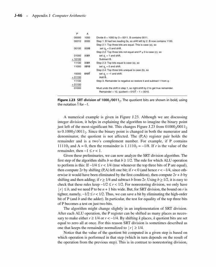
J-46 ■ Appendix J Computer Arithmetic
A numerical example is given in Figure J.23. Although we are discussinginteger division, it helps in explaining the algorithm to imagine the binary pointjust left of the most-significant bit. This changes Figure J.23 from 010002/00112to 0.10002/.00112. Since the binary point is changed in both the numerator anddenominator, the quotient is not affected. The (P,A) register pair holds theremainder and is a two’s complement number. For example, if P contains111102 and A = 0, then the remainder is 1.11102 = −1/8. If r is the value of theremainder, then −1 ≤ r < 1.
Given these preliminaries, we can now analyze the SRT division algorithm. Thefirst step of the algorithm shifts b so that b ≥ 1/2. The rule for which ALU operationto perform is this: If −1/4 ≤ r < 1/4 (true whenever the top three bits of P are equal),then compute 2r by shifting (P,A) left one bit; if r < 0 (and hence r < −1/4, since oth-erwise it would have been eliminated by the first condition), then compute 2r + b byshifting and then adding; if r ≥ 1/4 and subtract b from 2r. Using b ≥ 1/2, it is easy tocheck that these rules keep −1/2 ≤ r < 1/2. For nonrestoring division, we only have
⏐r⏐ ≤ b, and we need P to be n + 1 bits wide. But, for SRT division, the bound on r istighter, namely, −1/2 ≤ r < 1/2. Thus, we can save a bit by eliminating the high-orderbit of P (and b and the adder). In particular, the test for equality of the top three bitsof P becomes a test on just two bits.
The algorithm might change slightly in an implementation of SRT division.After each ALU operation, the P register can be shifted as many places as neces-sary to make either r ≥ 1/4 or r < −1/4. By shifting k places, k quotient bits are setequal to zero all at once. For this reason SRT division is sometimes described asone that keeps the remainder normalized to ⏐r⏐ ≥ 1/4.
Notice that the value of the quotient bit computed in a given step is based onwhich operation is performed in that step (which in turn depends on the result ofthe operation from the previous step). This is in contrast to nonrestoring division,
Figure J.23 SRT division of 10002/00112. The quotient bits are shown in bold, usingthe notation 1 for −1.
0000000010
00100
01000+ 10100
1110011000
10000+ 01100
11100+ 01100
01000
10000000
0000
0001
00010010
0101
Divide 8 = 1000 by 3 = 0011. B contains 0011.Step 1: B had two leading 0s, so shift left by 2. B now contains 1100.Step 2.1: Top three bits are equal. This is case (a), so set q
0 = 0 and shift.
Step 2.2: Top three bits not equal and P > 0 is case (c), so set q
1 = 1 and shift.
Subtract B.Step 2.3: Top bits equal is case (a), so set q
2 = 0 and shift.
Step 2.4: Top three bits unequal is case (b), so set q
3 = –1 and shift.
Add B.Step 3. Remainder is negative so restore it and subtract 1 from q.
Must undo the shift in step 1, so right-shift by 2 to get true remainder. Remainder = 10, quotient = 0101 – 1 = 0010.
P A
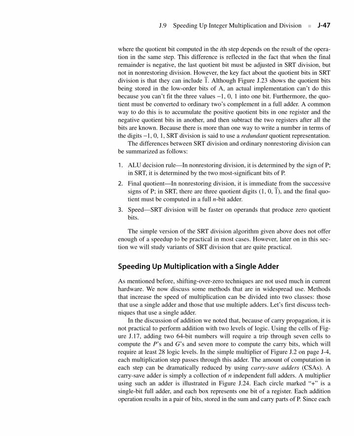
J.9 Speeding Up Integer Multiplication and Division ■ J-47
where the quotient bit computed in the ith step depends on the result of the opera-tion in the same step. This difference is reflected in the fact that when the finalremainder is negative, the last quotient bit must be adjusted in SRT division, butnot in nonrestoring division. However, the key fact about the quotient bits in SRTdivision is that they can include 1. Although Figure J.23 shows the quotient bitsbeing stored in the low-order bits of A, an actual implementation can’t do thisbecause you can’t fit the three values −1, 0, 1 into one bit. Furthermore, the quo-tient must be converted to ordinary two’s complement in a full adder. A commonway to do this is to accumulate the positive quotient bits in one register and thenegative quotient bits in another, and then subtract the two registers after all thebits are known. Because there is more than one way to write a number in terms ofthe digits −1, 0, 1, SRT division is said to use a redundant quotient representation.
The differences between SRT division and ordinary nonrestoring division canbe summarized as follows:
1. ALU decision rule—In nonrestoring division, it is determined by the sign of P;in SRT, it is determined by the two most-significant bits of P.
2. Final quotient—In nonrestoring division, it is immediate from the successivesigns of P; in SRT, there are three quotient digits (1, 0, 1), and the final quo-tient must be computed in a full n-bit adder.
3. Speed—SRT division will be faster on operands that produce zero quotientbits.
The simple version of the SRT division algorithm given above does not offerenough of a speedup to be practical in most cases. However, later on in this sec-tion we will study variants of SRT division that are quite practical.
Speeding Up Multiplication with a Single Adder
As mentioned before, shifting-over-zero techniques are not used much in currenthardware. We now discuss some methods that are in widespread use. Methodsthat increase the speed of multiplication can be divided into two classes: thosethat use a single adder and those that use multiple adders. Let’s first discuss tech-niques that use a single adder.
In the discussion of addition we noted that, because of carry propagation, it isnot practical to perform addition with two levels of logic. Using the cells of Fig-ure J.17, adding two 64-bit numbers will require a trip through seven cells tocompute the P’s and G’s and seven more to compute the carry bits, which willrequire at least 28 logic levels. In the simple multiplier of Figure J.2 on page J-4,each multiplication step passes through this adder. The amount of computation ineach step can be dramatically reduced by using carry-save adders (CSAs). Acarry-save adder is simply a collection of n independent full adders. A multiplierusing such an adder is illustrated in Figure J.24. Each circle marked “+” is asingle-bit full adder, and each box represents one bit of a register. Each additionoperation results in a pair of bits, stored in the sum and carry parts of P. Since each
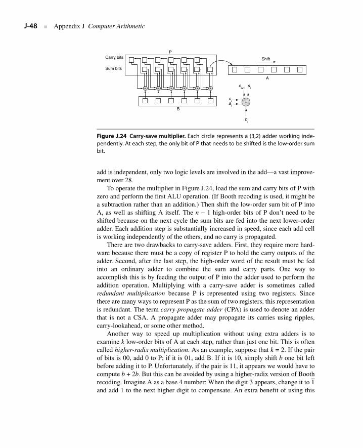
J-48 ■ Appendix J Computer Arithmetic
add is independent, only two logic levels are involved in the add—a vast improve-ment over 28.
To operate the multiplier in Figure J.24, load the sum and carry bits of P withzero and perform the first ALU operation. (If Booth recoding is used, it might bea subtraction rather than an addition.) Then shift the low-order sum bit of P intoA, as well as shifting A itself. The n − 1 high-order bits of P don’t need to beshifted because on the next cycle the sum bits are fed into the next lower-orderadder. Each addition step is substantially increased in speed, since each add cellis working independently of the others, and no carry is propagated.
There are two drawbacks to carry-save adders. First, they require more hard-ware because there must be a copy of register P to hold the carry outputs of theadder. Second, after the last step, the high-order word of the result must be fedinto an ordinary adder to combine the sum and carry parts. One way toaccomplish this is by feeding the output of P into the adder used to perform theaddition operation. Multiplying with a carry-save adder is sometimes calledredundant multiplication because P is represented using two registers. Sincethere are many ways to represent P as the sum of two registers, this representationis redundant. The term carry-propagate adder (CPA) is used to denote an adderthat is not a CSA. A propagate adder may propagate its carries using ripples,carry-lookahead, or some other method.
Another way to speed up multiplication without using extra adders is toexamine k low-order bits of A at each step, rather than just one bit. This is oftencalled higher-radix multiplication. As an example, suppose that k = 2. If the pairof bits is 00, add 0 to P; if it is 01, add B. If it is 10, simply shift b one bit leftbefore adding it to P. Unfortunately, if the pair is 11, it appears we would have tocompute b + 2b. But this can be avoided by using a higher-radix version of Boothrecoding. Imagine A as a base 4 number: When the digit 3 appears, change it to 1and add 1 to the next higher digit to compensate. An extra benefit of using this
Figure J.24 Carry-save multiplier. Each circle represents a (3,2) adder working inde-pendently. At each step, the only bit of P that needs to be shifted is the low-order sumbit.
B
A
P
Sum bits
Carry bits
ci
ai
ci+1
si
bi
Shift
+ + + + + +
+
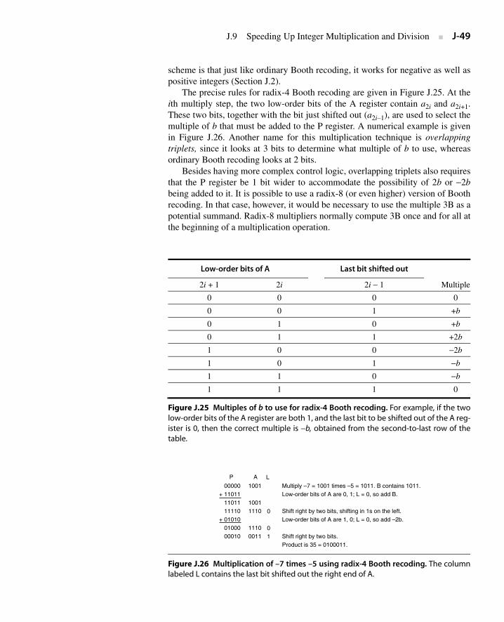
J.9 Speeding Up Integer Multiplication and Division ■ J-49
scheme is that just like ordinary Booth recoding, it works for negative as well aspositive integers (Section J.2).
The precise rules for radix-4 Booth recoding are given in Figure J.25. At theith multiply step, the two low-order bits of the A register contain a2i and a2i+1.These two bits, together with the bit just shifted out (a2i–1), are used to select themultiple of b that must be added to the P register. A numerical example is givenin Figure J.26. Another name for this multiplication technique is overlappingtriplets, since it looks at 3 bits to determine what multiple of b to use, whereasordinary Booth recoding looks at 2 bits.
Besides having more complex control logic, overlapping triplets also requiresthat the P register be 1 bit wider to accommodate the possibility of 2b or −2bbeing added to it. It is possible to use a radix-8 (or even higher) version of Boothrecoding. In that case, however, it would be necessary to use the multiple 3B as apotential summand. Radix-8 multipliers normally compute 3B once and for all atthe beginning of a multiplication operation.
Low-order bits of A Last bit shifted out
2i + 1 2i 2i − 1 Multiple
0 0 0 0
0 0 1 +b
0 1 0 +b
0 1 1 +2b
1 0 0 −2b
1 0 1 −b
1 1 0 −b
1 1 1 0
Figure J.25 Multiples of b to use for radix-4 Booth recoding. For example, if the twolow-order bits of the A register are both 1, and the last bit to be shifted out of the A reg-ister is 0, then the correct multiple is −b, obtained from the second-to-last row of thetable.
Figure J.26 Multiplication of –7 times –5 using radix-4 Booth recoding. The columnlabeled L contains the last bit shifted out the right end of A.
00000+ 11011
1101111110
+ 010100100000010
1001
10011110
11100011
Multiply –7 = 1001 times –5 = 1011. B contains 1011.Low-order bits of A are 0, 1; L = 0, so add B.
Shift right by two bits, shifting in 1s on the left.Low-order bits of A are 1, 0; L = 0, so add –2b.
Shift right by two bits.Product is 35 = 0100011.
P A
0
01
L
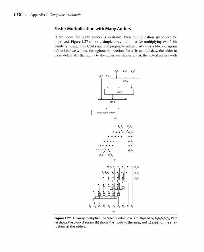
J-50 ■ Appendix J Computer Arithmetic
Faster Multiplication with Many Adders
If the space for many adders is available, then multiplication speed can beimproved. Figure J.27 shows a simple array multiplier for multiplying two 5-bitnumbers, using three CSAs and one propagate adder. Part (a) is a block diagramof the kind we will use throughout this section. Parts (b) and (c) show the adder inmore detail. All the inputs to the adder are shown in (b); the actual adders with
Figure J.27 An array multiplier. The 5-bit number in A is multiplied by b4b3b2b1b0. Part(a) shows the block diagram, (b) shows the inputs to the array, and (c) expands the arrayto show all the adders.
(b)
(c)
b0
a1
b0
a0
b0
A
b1
A
b2
A
b3
A
b4
A
b4
a1
b4
a0
b0
a4 b
0 A
b1
A
b2
A
b1
a4
p9
p8
p7
p6
p5
p4
p3
p2
p1
p0
(a)
b4A b
3A
b2A b
1A b
0A
CSA
CSA
CSA
Propagate adder
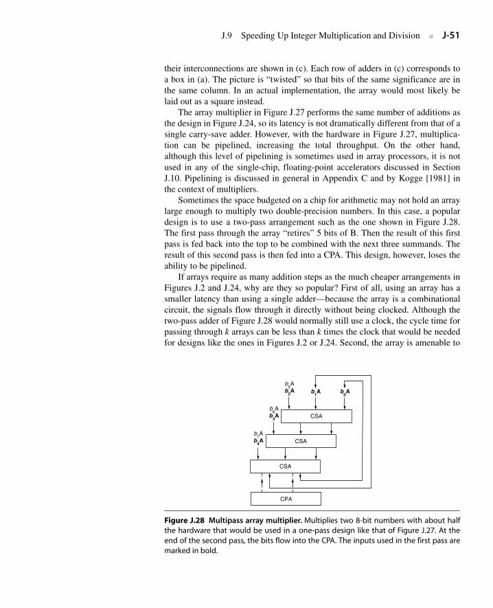
J.9 Speeding Up Integer Multiplication and Division ■ J-51
their interconnections are shown in (c). Each row of adders in (c) corresponds toa box in (a). The picture is “twisted” so that bits of the same significance are inthe same column. In an actual implementation, the array would most likely belaid out as a square instead.
The array multiplier in Figure J.27 performs the same number of additions asthe design in Figure J.24, so its latency is not dramatically different from that of asingle carry-save adder. However, with the hardware in Figure J.27, multiplica-tion can be pipelined, increasing the total throughput. On the other hand,although this level of pipelining is sometimes used in array processors, it is notused in any of the single-chip, floating-point accelerators discussed in SectionJ.10. Pipelining is discussed in general in Appendix C and by Kogge [1981] inthe context of multipliers.
Sometimes the space budgeted on a chip for arithmetic may not hold an arraylarge enough to multiply two double-precision numbers. In this case, a populardesign is to use a two-pass arrangement such as the one shown in Figure J.28.The first pass through the array “retires” 5 bits of B. Then the result of this firstpass is fed back into the top to be combined with the next three summands. Theresult of this second pass is then fed into a CPA. This design, however, loses theability to be pipelined.
If arrays require as many addition steps as the much cheaper arrangements inFigures J.2 and J.24, why are they so popular? First of all, using an array has asmaller latency than using a single adder—because the array is a combinationalcircuit, the signals flow through it directly without being clocked. Although thetwo-pass adder of Figure J.28 would normally still use a clock, the cycle time forpassing through k arrays can be less than k times the clock that would be neededfor designs like the ones in Figures J.2 or J.24. Second, the array is amenable to
Figure J.28 Multipass array multiplier. Multiplies two 8-bit numbers with about halfthe hardware that would be used in a one-pass design like that of Figure J.27. At theend of the second pass, the bits flow into the CPA. The inputs used in the first pass aremarked in bold.
CSA
CPA
b5A
b2A
b6A
b3A
b7A
b4A
b1A b
0A
CSA
CSA
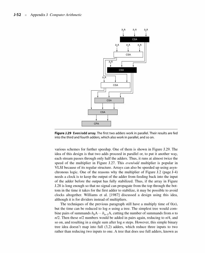
J-52 ■ Appendix J Computer Arithmetic
various schemes for further speedup. One of them is shown in Figure J.29. Theidea of this design is that two adds proceed in parallel or, to put it another way,each stream passes through only half the adders. Thus, it runs at almost twice thespeed of the multiplier in Figure J.27. This even/odd multiplier is popular inVLSI because of its regular structure. Arrays can also be speeded up using asyn-chronous logic. One of the reasons why the multiplier of Figure J.2 (page J-4)needs a clock is to keep the output of the adder from feeding back into the inputof the adder before the output has fully stabilized. Thus, if the array in FigureJ.28 is long enough so that no signal can propagate from the top through the bot-tom in the time it takes for the first adder to stabilize, it may be possible to avoidclocks altogether. Williams et al. [1987] discussed a design using this idea,although it is for dividers instead of multipliers.
The techniques of the previous paragraph still have a multiply time of 0(n),but the time can be reduced to log n using a tree. The simplest tree would com-bine pairs of summands b0A ⋅⋅⋅ bn–1A, cutting the number of summands from n ton/2. Then these n/2 numbers would be added in pairs again, reducing to n/4, andso on, and resulting in a single sum after log n steps. However, this simple binarytree idea doesn’t map into full (3,2) adders, which reduce three inputs to tworather than reducing two inputs to one. A tree that does use full adders, known as
Figure J.29 Even/odd array. The first two adders work in parallel. Their results are fedinto the third and fourth adders, which also work in parallel, and so on.
b2A
b4A b
3Ab
5A
b1A b
0A
CSA
CSA
b6A
b7A
CSA
CSA
CSA
CPA
CSA
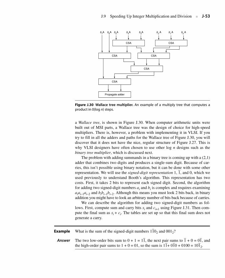
J.9 Speeding Up Integer Multiplication and Division ■ J-53
a Wallace tree, is shown in Figure J.30. When computer arithmetic units werebuilt out of MSI parts, a Wallace tree was the design of choice for high-speedmultipliers. There is, however, a problem with implementing it in VLSI. If youtry to fill in all the adders and paths for the Wallace tree of Figure J.30, you willdiscover that it does not have the nice, regular structure of Figure J.27. This iswhy VLSI designers have often chosen to use other log n designs such as thebinary tree multiplier, which is discussed next.
The problem with adding summands in a binary tree is coming up with a (2,1)adder that combines two digits and produces a single-sum digit. Because of car-ries, this isn’t possible using binary notation, but it can be done with some otherrepresentation. We will use the signed-digit representation 1, 1, and 0, which weused previously to understand Booth’s algorithm. This representation has twocosts. First, it takes 2 bits to represent each signed digit. Second, the algorithmfor adding two signed-digit numbers ai and bi is complex and requires examiningaiai–1ai–2 and bibi–1bi–2. Although this means you must look 2 bits back, in binaryaddition you might have to look an arbitrary number of bits back because of carries.
We can describe the algorithm for adding two signed-digit numbers as fol-lows. First, compute sum and carry bits si and ci+1 using Figure J.31. Then com-pute the final sum as si + ci. The tables are set up so that this final sum does notgenerate a carry.
Example What is the sum of the signed-digit numbers 1102 and 0012?
Answer The two low-order bits sum to 0 + 1 = 11, the next pair sums to 1 + 0 = 01, andthe high-order pair sums to 1 + 0 = 01, so the sum is 11+ 010 + 0100 = 1012.
Figure J.30 Wallace tree multiplier. An example of a multiply tree that computes aproduct in 0(log n) steps.
CSA
CSA
CSA
CSA
b7A b
6A b
5A b
4A b
3A b
2 A b
1 A b
0 A
CSA
CSA
Propagate adder
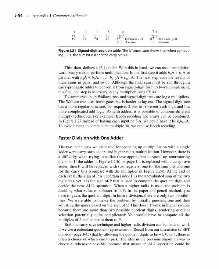
J-54 ■ Appendix J Computer Arithmetic
This, then, defines a (2,1) adder. With this in hand, we can use a straightfor-ward binary tree to perform multiplication. In the first step it adds b0A + b1A inparallel with b2A + b3A, . . . , bn–2A + bn–1A. The next step adds the results ofthese sums in pairs, and so on. Although the final sum must be run through acarry-propagate adder to convert it from signed-digit form to two’s complement,this final add step is necessary in any multiplier using CSAs.
To summarize, both Wallace trees and signed-digit trees are log n multipliers.The Wallace tree uses fewer gates but is harder to lay out. The signed-digit treehas a more regular structure, but requires 2 bits to represent each digit and hasmore complicated add logic. As with adders, it is possible to combine differentmultiply techniques. For example, Booth recoding and arrays can be combined.In Figure J.27 instead of having each input be biA, we could have it be bibi–1A.To avoid having to compute the multiple 3b, we can use Booth recoding.
Faster Division with One Adder
The two techniques we discussed for speeding up multiplication with a singleadder were carry-save adders and higher-radix multiplication. However, there isa difficulty when trying to utilize these approaches to speed up nonrestoringdivision. If the adder in Figure J.2(b) on page J-4 is replaced with a carry-saveadder, then P will be replaced with two registers, one for the sum bits and onefor the carry bits (compare with the multiplier in Figure J.24). At the end ofeach cycle, the sign of P is uncertain (since P is the unevaluated sum of the tworegisters), yet it is the sign of P that is used to compute the quotient digit anddecide the next ALU operation. When a higher radix is used, the problem isdeciding what value to subtract from P. In the paper-and-pencil method, youhave to guess the quotient digit. In binary division, there are only two possibil-ities. We were able to finesse the problem by initially guessing one and thenadjusting the guess based on the sign of P. This doesn’t work in higher radicesbecause there are more than two possible quotient digits, rendering quotientselection potentially quite complicated: You would have to compute all themultiples of b and compare them to P.
Both the carry-save technique and higher-radix division can be made to workif we use a redundant quotient representation. Recall from our discussion of SRTdivision (page J-45) that by allowing the quotient digits to be −1, 0, or 1, there isoften a choice of which one to pick. The idea in the previous algorithm was tochoose 0 whenever possible, because that meant an ALU operation could be
Figure J.31 Signed-digit addition table. The leftmost sum shows that when comput-ing 1 + 1, the sum bit is 0 and the carry bit is 1.
1+ 11 0
1+ 10 0
1+ 11 0
0+ 00 0
x
y1
+ 01 10 1
x
y1
+ 00 11 1
if 0 and 0otherwise
x ≥ y ≥ if 0 and 0otherwise
x ≥ y ≥
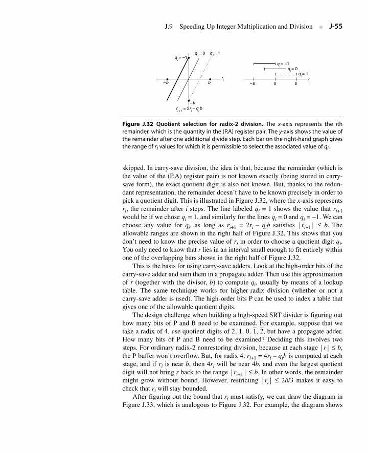
J.9 Speeding Up Integer Multiplication and Division ■ J-55
skipped. In carry-save division, the idea is that, because the remainder (which isthe value of the (P,A) register pair) is not known exactly (being stored in carry-save form), the exact quotient digit is also not known. But, thanks to the redun-dant representation, the remainder doesn’t have to be known precisely in order topick a quotient digit. This is illustrated in Figure J.32, where the x-axis representsri, the remainder after i steps. The line labeled qi = 1 shows the value that ri+1would be if we chose qi = 1, and similarly for the lines qi = 0 and qi = −1. We canchoose any value for qi, as long as ri+1 = 2ri – qib satisfies ⏐ri+1⏐ ≤ b. Theallowable ranges are shown in the right half of Figure J.32. This shows that youdon’t need to know the precise value of ri in order to choose a quotient digit qi.You only need to know that r lies in an interval small enough to fit entirely withinone of the overlapping bars shown in the right half of Figure J.32.
This is the basis for using carry-save adders. Look at the high-order bits of thecarry-save adder and sum them in a propagate adder. Then use this approximationof r (together with the divisor, b) to compute qi, usually by means of a lookuptable. The same technique works for higher-radix division (whether or not acarry-save adder is used). The high-order bits P can be used to index a table thatgives one of the allowable quotient digits.
The design challenge when building a high-speed SRT divider is figuring outhow many bits of P and B need to be examined. For example, suppose that wetake a radix of 4, use quotient digits of 2, 1, 0, 1, 2, but have a propagate adder.How many bits of P and B need to be examined? Deciding this involves twosteps. For ordinary radix-2 nonrestoring division, because at each stage ⏐r⏐ ≤ b,the P buffer won’t overflow. But, for radix 4, ri+1 = 4ri – qib is computed at eachstage, and if ri is near b, then 4ri will be near 4b, and even the largest quotientdigit will not bring r back to the range ⏐ri+1⏐ ≤ b. In other words, the remaindermight grow without bound. However, restricting ⏐ri⏐ ≤ 2b/3 makes it easy tocheck that ri will stay bounded.
After figuring out the bound that ri must satisfy, we can draw the diagram inFigure J.33, which is analogous to Figure J.32. For example, the diagram shows
Figure J.32 Quotient selection for radix-2 division. The x-axis represents the ithremainder, which is the quantity in the (P,A) register pair. The y-axis shows the value ofthe remainder after one additional divide step. Each bar on the right-hand graph givesthe range of ri values for which it is permissible to select the associated value of qi.
b–b
–b
b–b 0
qi = –1
qi = 0 q
i = 1
qi = –1
qi = 0
qi = 1
ri
ri
ri +1
= 2ri – q
ib
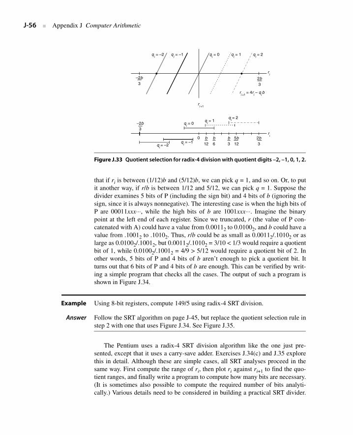
J-56 ■ Appendix J Computer Arithmetic
that if ri is between (1/12)b and (5/12)b, we can pick q = 1, and so on. Or, to putit another way, if r/b is between 1/12 and 5/12, we can pick q = 1. Suppose thedivider examines 5 bits of P (including the sign bit) and 4 bits of b (ignoring thesign, since it is always nonnegative). The interesting case is when the high bits ofP are 00011xxx⋅⋅⋅, while the high bits of b are 1001xxx⋅⋅⋅. Imagine the binarypoint at the left end of each register. Since we truncated, r (the value of P con-catenated with A) could have a value from 0.00112 to 0.01002, and b could have avalue from .10012 to .10102. Thus, r/b could be as small as 0.00112/.10102 or aslarge as 0.01002/.10012, but 0.00112/.10102 = 3/10 < 1/3 would require a quotientbit of 1, while 0.01002/.10012 = 4/9 > 5/12 would require a quotient bit of 2. Inother words, 5 bits of P and 4 bits of b aren’t enough to pick a quotient bit. Itturns out that 6 bits of P and 4 bits of b are enough. This can be verified by writ-ing a simple program that checks all the cases. The output of such a program isshown in Figure J.34.
Example Using 8-bit registers, compute 149/5 using radix-4 SRT division.
Answer Follow the SRT algorithm on page J-45, but replace the quotient selection rule instep 2 with one that uses Figure J.34. See Figure J.35.
The Pentium uses a radix-4 SRT division algorithm like the one just pre-sented, except that it uses a carry-save adder. Exercises J.34(c) and J.35 explorethis in detail. Although these are simple cases, all SRT analyses proceed in thesame way. First compute the range of ri, then plot ri against ri+1 to find the quo-tient ranges, and finally write a program to compute how many bits are necessary.(It is sometimes also possible to compute the required number of bits analyti-cally.) Various details need to be considered in building a practical SRT divider.
Figure J.33 Quotient selection for radix-4 division with quotient digits –2, –1, 0, 1, 2.
2b3
–2b3
2b3
5b12
b3
b6
b12
0
qi = –2 q
i = –1 q
i = 1q
i = 0 q
i = 2
ri
ri +1
= 4ri – q
ib
qi = 2
qi = 1
ri
qi = 0
qi = –2
qi = –1
–2b3
ri +1
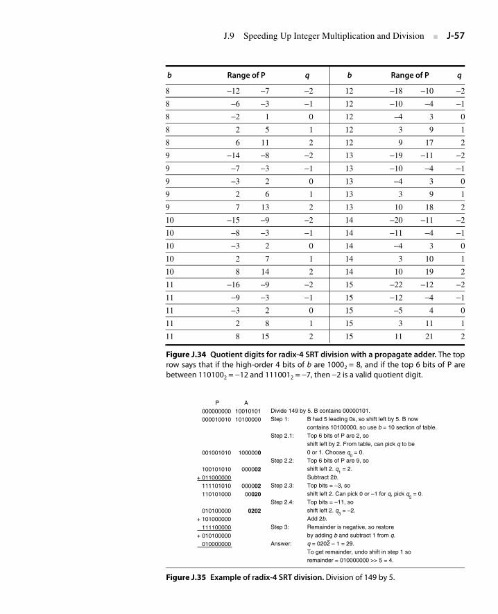
J.9 Speeding Up Integer Multiplication and Division ■ J-57
b Range of P q b Range of P q
8 −12 −7 −2 12 −18 −10 −2
8 −6 −3 −1 12 −10 −4 −1
8 −2 1 0 12 –4 3 0
8 2 5 1 12 3 9 1
8 6 11 2 12 9 17 2
9 −14 −8 −2 13 −19 −11 −2
9 −7 −3 −1 13 −10 −4 −1
9 −3 2 0 13 −4 3 0
9 2 6 1 13 3 9 1
9 7 13 2 13 10 18 2
10 −15 −9 −2 14 −20 −11 −2
10 −8 −3 −1 14 −11 −4 −1
10 −3 2 0 14 −4 3 0
10 2 7 1 14 3 10 1
10 8 14 2 14 10 19 2
11 −16 −9 −2 15 −22 −12 −2
11 −9 −3 −1 15 −12 −4 −1
11 −3 2 0 15 −5 4 0
11 2 8 1 15 3 11 1
11 8 15 2 15 11 21 2
Figure J.34 Quotient digits for radix-4 SRT division with a propagate adder. The toprow says that if the high-order 4 bits of b are 10002 = 8, and if the top 6 bits of P arebetween 1101002 = −12 and 1110012 = −7, then −2 is a valid quotient digit.
Figure J.35 Example of radix-4 SRT division. Division of 149 by 5.
000000000000010010
001001010
100101010+ 011000000
111101010110101000
010100000+ 101000000
111100000+ 010100000
010000000
A1001010110100000
1000000
000002
00000200020
0202
Divide 149 by 5. B contains 00000101.Step 1:
Step 2.1:
Step 2.2:
Step 2.3:
Step 2.4:
Step 3:
Answer:
B had 5 leading 0s, so shift left by 5. B nowcontains 10100000, so use b = 10 section of table.Top 6 bits of P are 2, soshift left by 2. From table, can pick q to be0 or 1. Choose q
0 = 0.
Top 6 bits of P are 9, soshift left 2. q
1 = 2.
Subtract 2b.Top bits = –3, soshift left 2. Can pick 0 or –1 for q, pick q
2 = 0.
Top bits = –11, soshift left 2. q
3 = –2.
Add 2b.Remainder is negative, so restoreby adding b and subtract 1 from q.q = 0202 – 1 = 29.To get remainder, undo shift in step 1 soremainder = 010000000 >> 5 = 4.
P
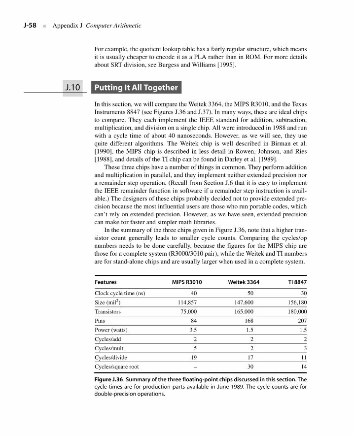
J-58 ■ Appendix J Computer Arithmetic
For example, the quotient lookup table has a fairly regular structure, which meansit is usually cheaper to encode it as a PLA rather than in ROM. For more detailsabout SRT division, see Burgess and Williams [1995].
In this section, we will compare the Weitek 3364, the MIPS R3010, and the TexasInstruments 8847 (see Figures J.36 and J.37). In many ways, these are ideal chipsto compare. They each implement the IEEE standard for addition, subtraction,multiplication, and division on a single chip. All were introduced in 1988 and runwith a cycle time of about 40 nanoseconds. However, as we will see, they usequite different algorithms. The Weitek chip is well described in Birman et al.[1990], the MIPS chip is described in less detail in Rowen, Johnson, and Ries[1988], and details of the TI chip can be found in Darley et al. [1989].
These three chips have a number of things in common. They perform additionand multiplication in parallel, and they implement neither extended precision nora remainder step operation. (Recall from Section J.6 that it is easy to implementthe IEEE remainder function in software if a remainder step instruction is avail-able.) The designers of these chips probably decided not to provide extended pre-cision because the most influential users are those who run portable codes, whichcan’t rely on extended precision. However, as we have seen, extended precisioncan make for faster and simpler math libraries.
In the summary of the three chips given in Figure J.36, note that a higher tran-sistor count generally leads to smaller cycle counts. Comparing the cycles/opnumbers needs to be done carefully, because the figures for the MIPS chip arethose for a complete system (R3000/3010 pair), while the Weitek and TI numbersare for stand-alone chips and are usually larger when used in a complete system.
Features MIPS R3010 Weitek 3364 TI 8847
Clock cycle time (ns) 40 50 30
Size (mil2) 114,857 147,600 156,180
Transistors 75,000 165,000 180,000
Pins 84 168 207
Power (watts) 3.5 1.5 1.5
Cycles/add 2 2 2
Cycles/mult 5 2 3
Cycles/divide 19 17 11
Cycles/square root – 30 14
Figure J.36 Summary of the three floating-point chips discussed in this section. Thecycle times are for production parts available in June 1989. The cycle counts are fordouble-precision operations.
J.10 Putting It All Together
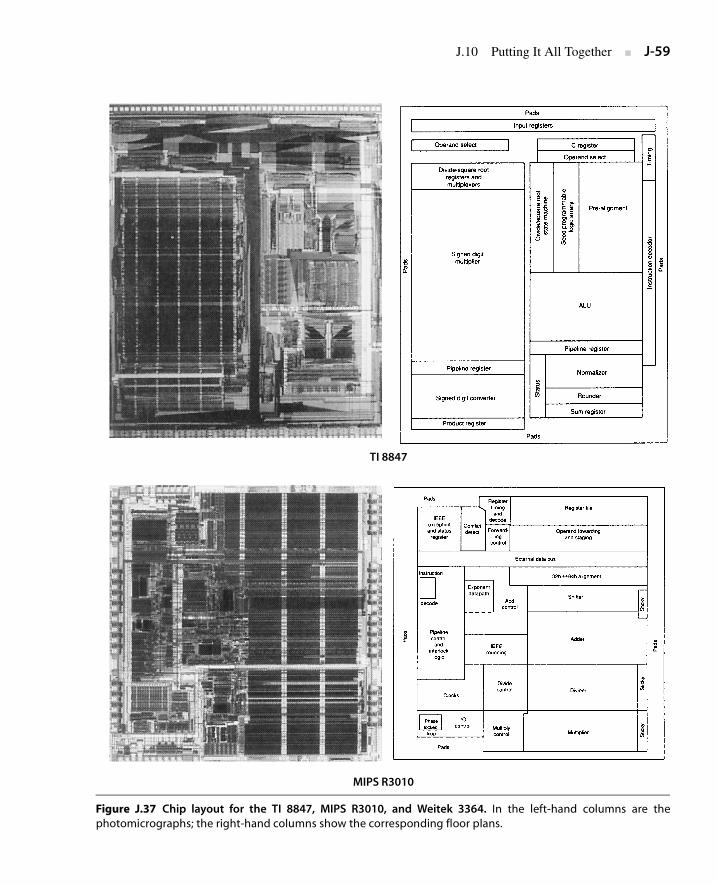
J.10 Putting It All Together ■ J-59
Figure J.37 Chip layout for the TI 8847, MIPS R3010, and Weitek 3364. In the left-hand columns are thephotomicrographs; the right-hand columns show the corresponding floor plans.
TI 8847
MIPS R3010
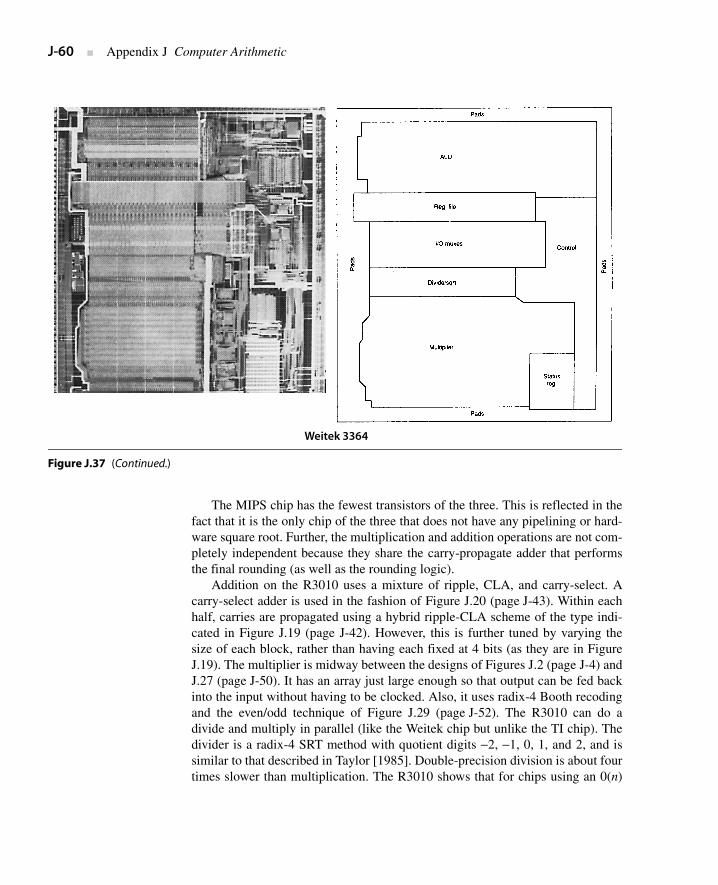
J-60 ■ Appendix J Computer Arithmetic
The MIPS chip has the fewest transistors of the three. This is reflected in thefact that it is the only chip of the three that does not have any pipelining or hard-ware square root. Further, the multiplication and addition operations are not com-pletely independent because they share the carry-propagate adder that performsthe final rounding (as well as the rounding logic).
Addition on the R3010 uses a mixture of ripple, CLA, and carry-select. Acarry-select adder is used in the fashion of Figure J.20 (page J-43). Within eachhalf, carries are propagated using a hybrid ripple-CLA scheme of the type indi-cated in Figure J.19 (page J-42). However, this is further tuned by varying thesize of each block, rather than having each fixed at 4 bits (as they are in FigureJ.19). The multiplier is midway between the designs of Figures J.2 (page J-4) andJ.27 (page J-50). It has an array just large enough so that output can be fed backinto the input without having to be clocked. Also, it uses radix-4 Booth recodingand the even/odd technique of Figure J.29 (page J-52). The R3010 can do adivide and multiply in parallel (like the Weitek chip but unlike the TI chip). Thedivider is a radix-4 SRT method with quotient digits −2, −1, 0, 1, and 2, and issimilar to that described in Taylor [1985]. Double-precision division is about fourtimes slower than multiplication. The R3010 shows that for chips using an 0(n)
Figure J.37 (Continued.)
Weitek 3364
J.10 Putting It All Together ■ J-61
multiplier, an SRT divider can operate fast enough to keep a reasonable ratiobetween multiply and divide.
The Weitek 3364 has independent add, multiply, and divide units. It also usesradix-4 SRT division. However, the add and multiply operations on the Weitekchip are pipelined. The three addition stages are (1) exponent compare, (2) addfollowed by shift (or vice versa), and (3) final rounding. Stages (1) and (3) takeonly a half-cycle, allowing the whole operation to be done in two cycles, eventhough there are three pipeline stages. The multiplier uses an array of the style ofFigure J.28 but uses radix-8 Booth recoding, which means it must compute 3times the multiplier. The three multiplier pipeline stages are (1) compute 3b, (2)pass through array, and (3) final carry-propagation add and round. Single preci-sion passes through the array once, double precision twice. Like addition, thelatency is two cycles.
The Weitek chip uses an interesting addition algorithm. It is a variant on thecarry-skip adder pictured in Figure J.18 (page J-42). However, Pij, which is thelogical AND of many terms, is computed by rippling, performing one AND perripple. Thus, while the carries propagate left within a block, the value of Pij ispropagating right within the next block, and the block sizes are chosen so thatboth waves complete at the same time. Unlike the MIPS chip, the 3364 hashardware square root, which shares the divide hardware. The ratio of double-precision multiply to divide is 2:17. The large disparity between multiply anddivide is due to the fact that multiplication uses radix-8 Booth recoding, whiledivision uses a radix-4 method. In the MIPS R3010, multiplication and divisionuse the same radix.
The notable feature of the TI 8847 is that it does division by iteration (usingthe Goldschmidt algorithm discussed in Section J.6). This improves the speed ofdivision (the ratio of multiply to divide is 3:11), but means that multiplication anddivision cannot be done in parallel as on the other two chips. Addition has a two-stage pipeline. Exponent compare, fraction shift, and fraction addition are donein the first stage, normalization and rounding in the second stage. Multiplicationuses a binary tree of signed-digit adders and has a three-stage pipeline. The firststage passes through the array, retiring half the bits; the second stage passesthrough the array a second time; and the third stage converts from signed-digitform to two’s complement. Since there is only one array, a new multiply opera-tion can only be initiated in every other cycle. However, by slowing down theclock, two passes through the array can be made in a single cycle. In this case, anew multiplication can be initiated in each cycle. The 8847 adder uses a carry-select algorithm rather than carry-lookahead. As mentioned in Section J.6, the TIcarries 60 bits of precision in order to do correctly rounded division.
These three chips illustrate the different trade-offs made by designers withsimilar constraints. One of the most interesting things about these chips is thediversity of their algorithms. Each uses a different add algorithm, as well as a dif-ferent multiply algorithm. In fact, Booth recoding is the only technique that isuniversally used by all the chips.
J-62 ■ Appendix J Computer Arithmetic
Fallacy Underflows rarely occur in actual floating-point application code.
Although most codes rarely underflow, there are actual codes that underflow fre-quently. SDRWAVE [Kahaner 1988], which solves a one-dimensional waveequation, is one such example. This program underflows quite frequently, evenwhen functioning properly. Measurements on one machine show that addinghardware support for gradual underflow would cause SDRWAVE to run about50% faster.
Fallacy Conversions between integer and floating point are rare.
In fact, in spice they are as frequent as divides. The assumption that conversionsare rare leads to a mistake in the SPARC version 8 instruction set, which does notprovide an instruction to move from integer registers to floating-point registers.
Pitfall Don’t increase the speed of a floating-point unit without increasing its memorybandwidth.
A typical use of a floating-point unit is to add two vectors to produce a third vec-tor. If these vectors consist of double-precision numbers, then each floating-pointadd will use three operands of 64 bits each, or 24 bytes of memory. The memorybandwidth requirements are even greater if the floating-point unit can performaddition and multiplication in parallel (as most do).
Pitfall −x is not the same as 0 − x.
This is a fine point in the IEEE standard that has tripped up some designers.Because floating-point numbers use the sign magnitude system, there are twozeros, +0 and −0. The standard says that 0 − 0 = +0, whereas −(0) = −0. Thus, −xis not the same as 0 − x when x = 0.
The earliest computers used fixed point rather than floating point. In “Prelimi-nary Discussion of the Logical Design of an Electronic Computing Instrument,”Burks, Goldstine, and von Neumann [1946] put it like this:
There appear to be two major purposes in a “floating” decimal point system bothof which arise from the fact that the number of digits in a word is a constant fixedby design considerations for each particular machine. The first of these purposesis to retain in a sum or product as many significant digits as possible and the sec-ond of these is to free the human operator from the burden of estimating andinserting into a problem “scale factors”—multiplicative constants which serve tokeep numbers within the limits of the machine.
J.11 Fallacies and Pitfalls
J.12 Historical Perspective and References
J.12 Historical Perspective and References ■ J-63
There is, of course, no denying the fact that human time is consumed inarranging for the introduction of suitable scale factors. We only argue that thetime so consumed is a very small percentage of the total time we will spend inpreparing an interesting problem for our machine. The first advantage of the float-ing point is, we feel, somewhat illusory. In order to have such a floating point, onemust waste memory capacity that could otherwise be used for carrying more dig-its per word. It would therefore seem to us not at all clear whether the modestadvantages of a floating binary point offset the loss of memory capacity and theincreased complexity of the arithmetic and control circuits.
This enables us to see things from the perspective of early computer design-ers, who believed that saving computer time and memory were more importantthan saving programmer time.
The original papers introducing the Wallace tree, Booth recoding, SRT divi-sion, overlapped triplets, and so on are reprinted in Swartzlander [1990]. A goodexplanation of an early machine (the IBM 360/91) that used a pipelined Wallacetree, Booth recoding, and iterative division is in Anderson et al. [1967]. A discus-sion of the average time for single-bit SRT division is in Freiman [1961]; this isone of the few interesting historical papers that does not appear in Swartzlander.
The standard book of Mead and Conway [1980] discouraged the use of CLAsas not being cost effective in VLSI. The important paper by Brent and Kung[1982] helped combat that view. An example of a detailed layout for CLAs canbe found in Ngai and Irwin [1985] or in Weste and Eshraghian [1993], and amore theoretical treatment is given by Leighton [1992]. Takagi, Yasuura, andYajima [1985] provide a detailed description of a signed-digit tree multiplier.
Before the ascendancy of IEEE arithmetic, many different floating-point for-mats were in use. Three important ones were used by the IBM 370, the DECVAX, and the Cray. Here is a brief summary of these older formats. The VAXformat is closest to the IEEE standard. Its single-precision format (F format) islike IEEE single precision in that it has a hidden bit, 8 bits of exponent, and 23bits of fraction. However, it does not have a sticky bit, which causes it to roundhalfway cases up instead of to even. The VAX has a slightly different exponentrange from IEEE single: Emin is −128 rather than −126 as in IEEE, and Emax is126 instead of 127. The main differences between VAX and IEEE are the lack ofspecial values and gradual underflow. The VAX has a reserved operand, but itworks like a signaling NaN: It traps whenever it is referenced. Originally, theVAX’s double precision (D format) also had 8 bits of exponent. However, as thisis too small for many applications, a G format was added; like the IEEE standard,this format has 11 bits of exponent. The VAX also has an H format, which is 128bits long.
The IBM 370 floating-point format uses base 16 rather than base 2. Thismeans it cannot use a hidden bit. In single precision, it has 7 bits of exponent and24 bits (6 hex digits) of fraction. Thus, the largest representable number is1627 = 24 × 27 = 229, compared with 228 for IEEE. However, a number that is nor-malized in the hexadecimal sense only needs to have a nonzero leading digit.When interpreted in binary, the three most-significant bits could be zero. Thus,there are potentially fewer than 24 bits of significance. The reason for using the
J-64 ■ Appendix J Computer Arithmetic
higher base was to minimize the amount of shifting required when addingfloating-point numbers. However, this is less significant in current machines,where the floating-point add time is usually fixed independently of the operands.Another difference between 370 arithmetic and IEEE arithmetic is that the 370has neither a round digit nor a sticky digit, which effectively means that it trun-cates rather than rounds. Thus, in many computations, the result will systemati-cally be too small. Unlike the VAX and IEEE arithmetic, every bit pattern is avalid number. Thus, library routines must establish conventions for what to returnin case of errors. In the IBM FORTRAN library, for example, returns 2!
Arithmetic on Cray computers is interesting because it is driven by a motiva-tion for the highest possible floating-point performance. It has a 15-bit exponentfield and a 48-bit fraction field. Addition on Cray computers does not have aguard digit, and multiplication is even less accurate than addition. Thinking ofmultiplication as a sum of p numbers, each 2p bits long, Cray computers drop thelow-order bits of each summand. Thus, analyzing the exact error characteristics ofthe multiply operation is not easy. Reciprocals are computed using iteration, anddivision of a by b is done by multiplying a times 1/b. The errors in multiplicationand reciprocation combine to make the last three bits of a divide operationunreliable. At least Cray computers serve to keep numerical analysts on their toes!
The IEEE standardization process began in 1977, inspired mainly byW. Kahan and based partly on Kahan’s work with the IBM 7094 at the Universityof Toronto [Kahan 1968]. The standardization process was a lengthy affair, withgradual underflow causing the most controversy. (According to Cleve Moler, vis-itors to the United States were advised that the sights not to be missed were LasVegas, the Grand Canyon, and the IEEE standards committee meeting.) The stan-dard was finally approved in 1985. The Intel 8087 was the first major commercialIEEE implementation and appeared in 1981, before the standard was finalized. Itcontains features that were eliminated in the final standard, such as projectivebits. According to Kahan, the length of double-extended precision was based onwhat could be implemented in the 8087. Although the IEEE standard was notbased on any existing floating-point system, most of its features were present insome other system. For example, the CDC 6600 reserved special bit patterns forINDEFINITE and INFINITY, while the idea of denormal numbers appears inGoldberg [1967] as well as in Kahan [1968]. Kahan was awarded the 1989 Tur-ing prize in recognition of his work on floating point.
Although floating point rarely attracts the interest of the general press, news-papers were filled with stories about floating-point division in November 1994. Abug in the division algorithm used on all of Intel’s Pentium chips had just come tolight. It was discovered by Thomas Nicely, a math professor at Lynchburg Col-lege in Virginia. Nicely found the bug when doing calculations involving recipro-cals of prime numbers. News of Nicely’s discovery first appeared in the press onthe front page of the November 7 issue of Electronic Engineering Times. Intel’simmediate response was to stonewall, asserting that the bug would only affecttheoretical mathematicians. Intel told the press, “This doesn’t even qualify as anerrata . . . even if you’re an engineer, you’re not going to see this.”
4–
J.12 Historical Perspective and References ■ J-65
Under more pressure, Intel issued a white paper, dated November 30, explain-ing why they didn’t think the bug was significant. One of their arguments wasbased on the fact that if you pick two floating-point numbers at random anddivide one into the other, the chance that the resulting quotient will be in error isabout 1 in 9 billion. However, Intel neglected to explain why they thought that thetypical customer accessed floating-point numbers randomly.
Pressure continued to mount on Intel. One sore point was that Intel hadknown about the bug before Nicely discovered it, but had decided not to make itpublic. Finally, on December 20, Intel announced that they would uncondition-ally replace any Pentium chip that used the faulty algorithm and that they wouldtake an unspecified charge against earnings, which turned out to be $300 million.
The Pentium uses a simple version of SRT division as discussed in SectionJ.9. The bug was introduced when they converted the quotient lookup table to aPLA. Evidently there were a few elements of the table containing the quotientdigit 2 that Intel thought would never be accessed, and they optimized the PLAdesign using this assumption. The resulting PLA returned 0 rather than 2 in thesesituations. However, those entries were really accessed, and this caused the divi-sion bug. Even though the effect of the faulty PLA was to cause 5 out of 2048table entries to be wrong, the Pentium only computes an incorrect quotient 1 outof 9 billion times on random inputs. This is explored in Exercise J.34.
References
Anderson, S. F., J. G. Earle, R. E. Goldschmidt, and D. M. Powers [1967]. “The IBMSystem/360 Model 91: Floating-point execution unit,” IBM J. Research and Develop-ment 11, 34–53. Reprinted in Swartzlander [1990].Good description of an early high-performance floating-point unit that used a pipe-lined Wallace tree multiplier and iterative division.
Bell, C. G., and A. Newell [1971]. Computer Structures: Readings and Examples,McGraw-Hill, New York.
Birman, M., A. Samuels, G. Chu, T. Chuk, L. Hu, J. McLeod, and J. Barnes [1990].“Developing the WRL3170/3171 SPARC floating-point coprocessors,” IEEE Micro10:1, 55–64.These chips have the same floating-point core as the Weitek 3364, and this paper hasa fairly detailed description of that floating-point design.
Brent, R. P., and H. T. Kung [1982]. “A regular layout for parallel adders,” IEEE Trans.on Computers C-31, 260–264.This is the paper that popularized CLAs in VLSI.
Burgess, N., and T. Williams [1995]. “Choices of operand truncation in the SRT divisionalgorithm,” IEEE Trans. on Computers 44:7.Analyzes how many bits of divisor and remainder need to be examined in SRTdivision.
Burks, A. W., H. H. Goldstine, and J. von Neumann [1946]. “Preliminary discussion ofthe logical design of an electronic computing instrument,” Report to the U.S. ArmyOrdnance Department, p. 1; also appears in Papers of John von Neumann, W. Asprayand A. Burks, eds., MIT Press, Cambridge, Mass., and Tomash Publishers, LosAngeles, 1987, 97–146.
J-66 ■ Appendix J Computer Arithmetic
Cody, W. J., J. T. Coonen, D. M. Gay, K. Hanson, D. Hough, W. Kahan, R. Karpinski,J. Palmer, F. N. Ris, and D. Stevenson [1984]. “A proposed radix- and word-length-independent standard for floating-point arithmetic,” IEEE Micro 4:4, 86–100.Contains a draft of the 854 standard, which is more general than 754. The signifi-cance of this article is that it contains commentary on the standard, most of which isequally relevant to 754. However, be aware that there are some differences betweenthis draft and the final standard.
Coonen, J. [1984]. “Contributions to a proposed standard for binary floating point arith-metic,” Ph.D. thesis, University of California–Berkeley.The only detailed discussion of how rounding modes can be used to implement effi-cient binary decimal conversion.
Darley, H. M. et al. [1989]. “Floating point/integer processor with divide and square rootfunctions,” U.S. Patent 4,878,190, October 31, 1989.Pretty readable as patents go. Gives a high-level view of the TI 8847 chip, but doesn’thave all the details of the division algorithm.
Demmel, J. W., and X. Li [1994]. “Faster numerical algorithms via exception handling,”IEEE Trans. on Computers 43:8, 983–992.A good discussion of how the features unique to IEEE floating point can improve theperformance of an important software library.
Freiman, C. V. [1961]. “Statistical analysis of certain binary division algorithms,” Proc.IRE 49:1, 91–103.Contains an analysis of the performance of shifting-over-zeros SRT division algo-rithm.
Goldberg, D. [1991]. “What every computer scientist should know about floating-pointarithmetic,” Computing Surveys 23:1, 5–48.Contains an in-depth tutorial on the IEEE standard from the software point of view.
Goldberg, I. B. [1967]. “27 bits are not enough for 8-digit accuracy,” Comm. ACM 10:2,105–106.This paper proposes using hidden bits and gradual underflow.
Gosling, J. B. [1980]. Design of Arithmetic Units for Digital Computers, Springer-Verlag,New York.A concise, well-written book, although it focuses on MSI designs.
Hamacher, V. C., Z. G. Vranesic, and S. G. Zaky [1984]. Computer Organization, 2nd ed.,McGraw-Hill, New York.Introductory computer architecture book with a good chapter on computer arithmetic.
Hwang, K. [1979]. Computer Arithmetic: Principles, Architecture, and Design, Wiley,New York.This book contains the widest range of topics of the computer arithmetic books.
IEEE [1985]. “IEEE standard for binary floating-point arithmetic,” SIGPLAN Notices22:2, 9–25.IEEE 754 is reprinted here.
Kahan, W. [1968]. “7094-II system support for numerical analysis,” SHARE SecretarialDistribution SSD-159.This system had many features that were incorporated into the IEEE floating-pointstandard.
Kahaner, D. K. [1988]. “Benchmarks for ‘real’ programs,” SIAM News (November).The benchmark presented in this article turns out to cause many underflows.
J.12 Historical Perspective and References ■ J-67
Knuth, D. [1981]. The Art of Computer Programming, Vol. II, 2nd ed., Addison-Wesley,Reading, Mass.Has a section on the distribution of floating-point numbers.
Kogge, P. [1981]. The Architecture of Pipelined Computers, McGraw-Hill, New York.Has a brief discussion of pipelined multipliers.
Kohn, L., and S.-W. Fu [1989]. “A 1,000,000 transistor microprocessor,” IEEE Int’l.Solid-State Circuits Conf. Digest of Technical Papers, 54–55.There are several articles about the i860, but this one contains the most details aboutits floating-point algorithms.
Koren, I. [1989]. Computer Arithmetic Algorithms, Prentice Hall, Englewood Cliffs, N.J.Leighton, F. T. [1992]. Introduction to Parallel Algorithms and Architectures: Arrays,
Trees, Hypercubes, Morgan Kaufmann, San Francisco.This is an excellent book, with emphasis on the complexity analysis of algorithms.Section 1.2.1 has a nice discussion of carry-lookahead addition on a tree.
Magenheimer, D. J., L. Peters, K. W. Pettis, and D. Zuras [1988]. “Integer multiplicationand division on the HP Precision architecture,” IEEE Trans. on Computers 37:8,980–990.Gives rationale for the integer- and divide-step instructions in the Precision architecture.
Markstein, P. W. [1990]. “Computation of elementary functions on the IBM RISCSystem/6000 processor,” IBM J. of Research and Development 34:1, 111–119.Explains how to use fused muliply-add to compute correctly rounded division andsquare root.
Mead, C., and L. Conway [1980]. Introduction to VLSI Systems, Addison-Wesley, Read-ing, Mass.
Montoye, R. K., E. Hokenek, and S. L. Runyon [1990]. “Design of the IBM RISC System/6000 floating-point execution,” IBM J. of Research and Development 34:1, 59–70.Describes one implementation of fused multiply-add.
Ngai, T.-F., and M. J. Irwin [1985]. “Regular, area-time efficient carry-lookahead adders,”Proc. Seventh IEEE Symposium on Computer Arithmetic, 9–15.Describes a CLA like that of Figure J.17, where the bits flow up and then come backdown.
Patterson, D. A., and J. L. Hennessy [2009]. Computer Organization and Design: TheHardware/Software Interface, 4th Edition, Morgan Kaufmann, San Francisco.Chapter 3 is a gentler introduction to the first third of this appendix.
Peng, V., S. Samudrala, and M. Gavrielov [1987]. “On the implementation of shifters,multipliers, and dividers in VLSI floating point units,” Proc. Eighth IEEE Symposiumon Computer Arithmetic, 95–102.Highly recommended survey of different techniques actually used in VLSI designs.
Rowen, C., M. Johnson, and P. Ries [1988]. “The MIPS R3010 floating-point coproces-sor,” IEEE Micro, 53–62 (June).
Santoro, M. R., G. Bewick, and M. A. Horowitz [1989]. “Rounding algorithms for IEEEmultipliers,” Proc. Ninth IEEE Symposium on Computer Arithmetic, 176–183.A very readable discussion of how to efficiently implement rounding for floating-pointmultiplication.
Scott, N. R. [1985]. Computer Number Systems and Arithmetic, Prentice Hall, EnglewoodCliffs, N.J.
J-68 ■ Appendix J Computer Arithmetic
Swartzlander, E., ed. [1990]. Computer Arithmetic, IEEE Computer Society Press, LosAlamitos, Calif.A collection of historical papers in two volumes.
Takagi, N., H. Yasuura, and S. Yajima [1985].“High-speed VLSI multiplication algorithmwith a redundant binary addition tree,” IEEE Trans. on Computers C-34:9, 789–796.A discussion of the binary tree signed multiplier that was the basis for the design usedin the TI 8847.
Taylor, G. S. [1981]. “Compatible hardware for division and square root,” Proc. Fifth IEEESymposium on Computer Arithmetic, May 18–19, 1981, Ann Arbor, Mich., 127–134.Good discussion of a radix-4 SRT division algorithm.
Taylor, G. S. [1985]. “Radix 16 SRT dividers with overlapped quotient selection stages,” Proc.Seventh IEEE Symposium on Computer Arithmetic, June 4–6, 1985, Urbana, Ill., 64–71.Describes a very sophisticated high-radix division algorithm.
Weste, N., and K. Eshraghian [1993]. Principles of CMOS VLSI Design: A Systems Per-spective, 2nd ed., Addison-Wesley, Reading, Mass.This textbook has a section on the layouts of various kinds of adders.
Williams, T. E., M. Horowitz, R. L. Alverson, and T. S. Yang [1987]. “A self-timed chipfor division,” Advanced Research in VLSI, Proc. 1987 Stanford Conf., MIT Press,Cambridge, Mass.Describes a divider that tries to get the speed of a combinational design without usingthe area that would be required by one.
J.1 [12] <J.2> Using n bits, what is the largest and smallest integer that can be repre-sented in the two’s complement system?
J.2 [20/25] <J.2> In the subsection “Signed Numbers” (page J-7), it was stated thattwo’s complement overflows when the carry into the high-order bit position isdifferent from the carry-out from that position.
a. [20] <J.2> Give examples of pairs of integers for all four combinations ofcarry-in and carry-out. Verify the rule stated above.
b. [25] <J.2> Explain why the rule is always true.
J.3 [12] <J.2> Using 4-bit binary numbers, multiply −8 × −8 using Booth recoding.
J.4 [15] <J.2> Equations J.2.1 and J.2.2 are for adding two n-bit numbers. Derivesimilar equations for subtraction, where there will be a borrow instead of a carry.
J.5 [25] <J.2> On a machine that doesn’t detect integer overflow in hardware, showhow you would detect overflow on a signed addition operation in software.
J.6 [15/15/20] <J.3> Represent the following numbers as single-precision anddouble-precision IEEE floating-point numbers:
a. [15] <J.3> 10.
b. [15] <J.3> 10.5.
c. [20] <J.3> 0.1.
Exercises
Exercises ■ J-69
J.7 [12/12/12/12/12] <J.3> Below is a list of floating-point numbers. In single preci-sion, write down each number in binary, in decimal, and give its representation inIEEE arithmetic.
a. [12] <J.3> The largest number less than 1.
b. [12] <J.3> The largest number.
c. [12] <J.3> The smallest positive normalized number.
d. [12] <J.3> The largest denormal number.
e. [12] <J.3> The smallest positive number.
J.8 [15] <J.3> Is the ordering of nonnegative floating-point numbers the same asintegers when denormalized numbers are also considered?
J.9 [20] <J.3> Write a program that prints out the bit patterns used to representfloating-point numbers on your favorite computer. What bit pattern is used forNaN?
J.10 [15] <J.4> Using p = 4, show how the binary floating-point multiply algorithmcomputes the product of 1.875 × 1.875.
J.11 [12/10] <J.4> Concerning the addition of exponents in floating-point multiply:
a. [12] <J.4> What would the hardware that implements the addition of expo-nents look like?
b. [10] <J.4> If the bias in single precision were 129 instead of 127, would addi-tion be harder or easier to implement?
J.12 [15/12] <J.4> In the discussion of overflow detection for floating-point multipli-cation, it was stated that (for single precision) you can detect an overflowedexponent by performing exponent addition in a 9-bit adder.
a. [15] <J.4> Give the exact rule for detecting overflow.
b. [12] <J.4> Would overflow detection be any easier if you used a 10-bit adderinstead?
J.13 [15/10] <J.4> Floating-point multiplication:
a. [15] <J.4> Construct two single-precision floating-point numbers whoseproduct doesn’t overflow until the final rounding step.
b. [10] <J.4> Is there any rounding mode where this phenomenon cannot occur?
J.14 [15] <J.4> Give an example of a product with a denormal operand but a normal-ized output. How large was the final shifting step? What is the maximum possibleshift that can occur when the inputs are double-precision numbers?
J.15 [15] <J.5> Use the floating-point addition algorithm on page J-23 to compute1.0102 − .10012 (in 4-bit precision).
J.16 [10/15/20/20/20] <J.5> In certain situations, you can be sure that a + b is exactlyrepresentable as a floating-point number, that is, no rounding is necessary.
J-70 ■ Appendix J Computer Arithmetic
a. [10] <J.5> If a, b have the same exponent and different signs, explain whya + b is exact. This was used in the subsection “Speeding Up Addition” onpage J-25.
b. [15] <J.5> Give an example where the exponents differ by 1, a and b havedifferent signs, and a + b is not exact.
c. [20] <J.5> If a ≥ b ≥ 0, and the top two bits of a cancel when computing a – b,explain why the result is exact (this fact is mentioned on page J-22).
d. [20] <J.5> If a ≥ b ≥ 0, and the exponents differ by 1, show that a − b is exactunless the high order bit of a − b is in the same position as that of a (men-tioned in “Speeding Up Addition,” page J-25).
e. [20] <J.5> If the result of a − b or a + b is denormal, show that the result isexact (mentioned in the subsection “Underflow,” on page J-36).
J.17 [15/20] <J.5> Fast floating-point addition (using parallel adders) for p = 5.
a. [15] <J.5> Step through the fast addition algorithm for a + b, where a =1.01112 and b = .110112.
b. [20] <J.5> Suppose the rounding mode is toward +∞. What complicationarises in the above example for the adder that assumes a carry-out? Suggest asolution.
J.18 [12] <J.4, J.5> How would you use two parallel adders to avoid the final round-up addition in floating-point multiplication?
J.19 [30/10] <J.5> This problem presents a way to reduce the number of additionsteps in floating-point addition from three to two using only a single adder.
a. [30] <J.5> Let A and B be integers of opposite signs, with a and b their mag-nitudes. Show that the following rules for manipulating the unsigned numbersa and b gives A + B.
1. Complement one of the operands.
2. Use end-around carry to add the complemented operand and the other(uncomplemented) one.
3. If there was a carry-out, the sign of the result is the sign associated with theuncomplemented operand.
4. Otherwise, if there was no carry-out, complement the result, and give it thesign of the complemented operand.
b. [10] <J.5> Use the above to show how steps 2 and 4 in the floating-point addi-tion algorithm on page J-23 can be performed using only a single addition.
J.20 [20/15/20/15/20/15] <J.6> Iterative square root.
a. [20] <J.6> Use Newton’s method to derive an iterative algorithm for squareroot. The formula will involve a division.
b. [15] <J.6> What is the fastest way you can think of to divide a floating-pointnumber by 2?
Exercises ■ J-71
c. [20] <J.6> If division is slow, then the iterative square root routine will alsobe slow. Use Newton’s method on f(x) = 1/x2 − a to derive a method thatdoesn’t use any divisions.
d. [15] <J.6> Assume that the ratio division by 2 : floating-point add : floating-point multiply is 1:2:4. What ratios of multiplication time to divide timemakes each iteration step in the method of part (c) faster than each iteration inthe method of part (a)?
e. [20] <J.6> When using the method of part (a), how many bits need to be inthe initial guess in order to get double-precision accuracy after three itera-tions? (You may ignore rounding error.)
f. [15] <J.6> Suppose that when spice runs on the TI 8847, it spends 16.7% ofits time in the square root routine (this percentage has been measured onother machines). Using the values in Figure J.36 and assuming three itera-tions, how much slower would spice run if square root were implemented insoftware using the method of part(a)?
J.21 [10/20/15/15/15] <J.6> Correctly rounded iterative division. Let a and b befloating-point numbers with p-bit significands (p = 53 in double precision). Let qbe the exact quotient q = a/b, 1 ≤ q < 2. Suppose that q is the result of an iterationprocess, that q has a few extra bits of precision, and that 0 < q − q < 2–p. For thefollowing, it is important that q < q, even when q can be exactly represented as afloating-point number.
a. [10] <J.6> If x is a floating-point number, and 1 ≤ x < 2, what is the next rep-resentable number after x?
b. [20] <J.6> Show how to compute q′ from q, where q′ has p + 1 bits of preci-sion and ⏐q − q′ ⏐ < 2–p.
c. [15] <J.6> Assuming round to nearest, show that the correctly rounded quo-tient is either q′, q′ − 2–p, or q′ + 2–p.
d. [15] <J.6> Give rules for computing the correctly rounded quotient from q′based on the low-order bit of q′ and the sign of a − bq′.
e. [15] <J.6> Solve part (c) for the other three rounding modes.
J.22 [15] <J.6> Verify the formula on page J-30. (Hint: If xn = x0(2 − x0b) × Πi=1, n [1 +(1 − x0b)2i], then 2 − xnb = 2 − x0b(2 − x0b) Π[1 + (1 − x0b)2i] = 2 − [1 − (1 − x0b)2]
Π[1 + (1 − x0b)2i].)
J.23 [15] <J.7> Our example that showed that double rounding can give a differentanswer from rounding once used the round-to-even rule. If halfway cases arealways rounded up, is double rounding still dangerous?
J.24 [10/10/20/20] <J.7> Some of the cases of the italicized statement in the “Preci-sions” subsection (page J-33) aren’t hard to demonstrate.
a. [10] <J.7> What form must a binary number have if rounding to q bits fol-lowed by rounding to p bits gives a different answer than rounding directly top bits?
J-72 ■ Appendix J Computer Arithmetic
b. [10] <J.7> Show that for multiplication of p-bit numbers, rounding to q bitsfollowed by rounding to p bits is the same as rounding immediately to p bitsif q ≥ 2p.
c. [20] <J.7> If a and b are p-bit numbers with the same sign, show that round-ing a + b to q bits followed by rounding to p bits is the same as roundingimmediately to p bits if q ≥ 2p + 1.
d. [20] <J.7> Do part (c) when a and b have opposite signs.
J.25 [Discussion] <J.7> In the MIPS approach to exception handling, you need a testfor determining whether two floating-point operands could cause an exception.This should be fast and also not have too many false positives. Can you come upwith a practical test? The performance cost of your design will depend on the dis-tribution of floating-point numbers. This is discussed in Knuth [1981] and theHamming paper in Swartzlander [1990].
J.26 [12/12/10] <J.8> Carry-skip adders.
a. [12] <J.8> Assuming that time is proportional to logic levels, how long doesit take an n-bit adder divided into (fixed) blocks of length k bits to perform anaddition?
b. [12] <J.8> What value of k gives the fastest adder?
c. [10] <J.8> Explain why the carry-skip adder takes time .
J.27 [10/15/20] <J.8> Complete the details of the block diagrams for the followingadders.
a. [10] <J.8> In Figure J.15, show how to implement the “1” and “2” boxes interms of AND and OR gates.
b. [15] <J.8> In Figure J.19, what signals need to flow from the adder cells inthe top row into the “C” cells? Write the logic equations for the “C” box.
c. [20] <J.8> Show how to extend the block diagram in J.17 so it will producethe carry-out bit c8.
J.28 [15] <J.9> For ordinary Booth recoding, the multiple of b used in the ith step issimply ai–1 − ai. Can you find a similar formula for radix-4 Booth recoding (over-lapped triplets)?
J.29 [20] <J.9> Expand Figure J.29 in the fashion of J.27, showing the individualadders.
J.30 [25] <J.9> Write out the analog of Figure J.25 for radix-8 Booth recoding.
J.31 [18] <J.9> Suppose that an–1 . . . a1a0 and bn–1 . . . b1b0 are being added in asigned-digit adder as illustrated in the example on page J-53. Write a formula forthe ith bit of the sum, si, in terms of ai, ai–1, ai–2, bi, bi–1, and bi–2.
J.32 [15] <J.9> The text discussed radix-4 SRT division with quotient digits of −2, −1,0, 1, 2. Suppose that 3 and −3 are also allowed as quotient digits. What relationreplaces⏐ri⏐ ≤ 2b/3?
0 n( )
Exercises ■ J-73
J.33 [25/20/30] <J.9> Concerning the SRT division table, Figure J.34:
a. [25] <J.9> Write a program to generate the results of Figure J.34.
b. [20] <J.9> Note that Figure J.34 has a certain symmetry with respect to posi-tive and negative values of P. Can you find a way to exploit the symmetry andonly store the values for positive P?
c. [30] <J.9> Suppose a carry-save adder is used instead of a propagate adder.The input to the quotient lookup table will be k bits of divisor and l bits ofremainder, where the remainder bits are computed by summing the top l bitsof the sum and carry registers. What are k and l? Write a program to generatethe analog of Figure J.34.
J.34 [12/12/12] <J.9, J.12> The first several million Pentium chips produced had aflaw that caused division to sometimes return the wrong result. The Pentium usesa radix-4 SRT algorithm similar to the one illustrated in the example on page J-56(but with the remainder stored in carry-save format; see Exercise J.33(c)).According to Intel, the bug was due to five incorrect entries in the quotientlookup table.
a. [12] <J.9, J.12> The bad entries should have had a quotient of plus or minus2, but instead had a quotient of 0. Because of redundancy, it’s conceivablethat the algorithm could “recover” from a bad quotient digit on later itera-tions. Show that this is not possible for the Pentium flaw.
b. [12] <J.9, J.12> Since the operation is a floating-point divide rather than aninteger divide, the SRT division algorithm on page J-45 must be modified intwo ways. First, step 1 is no longer needed, since the divisor is already nor-malized. Second, the very first remainder may not satisfy the proper bound(⏐r ⏐≤ 2b/3 for Pentium; see page J-55). Show that skipping the very first leftshift in step 2(a) of the SRT algorithm will solve this problem.
c. [12] <J.9, J.12> If the faulty table entries were indexed by a remainder thatcould occur at the very first divide step (when the remainder is the divisor),random testing would quickly reveal the bug. This didn’t happen. What doesthat tell you about the remainder values that index the faulty entries?
J.35 [12] <J.6, J.9> The discussion of the remainder-step instruction assumed thatdivision was done using a bit-at-a-time algorithm. What would have to change ifdivision were implemented using a higher-radix method?
J.36 [25] <J.9> In the array of Figure J.28, the fact that an array can be pipelined is notexploited. Can you come up with a design that feeds the output of the bottomCSA into the bottom CSAs instead of the top one, and that will run faster than thearrangement of Figure J.28?


