
General rights Copyright and moral rights for the publications made accessible in the public portal are retained by the authors and/or other copyright owners and it is a condition of accessing publications that users recognise and abide by the legal requirements associated with these rights.
• Users may download and print one copy of any publication from the public portal for the purpose of private study or research. • You may not further distribute the material or use it for any profit-making activity or commercial gain • You may freely distribute the URL identifying the publication in the public portal
If you believe that this document breaches copyright please contact us providing details, and we will remove access to the work immediately and investigate your claim.
Downloaded from orbit.dtu.dk on: Jul 08, 2018
Coolant Mixing in Multirod Fuel Bundles
Forskningscenter Risø, Roskilde
Publication date:1966
Document VersionPublisher's PDF, also known as Version of record
Link back to DTU Orbit
Citation (APA):Moyer, C. B. (1966). Coolant Mixing in Multirod Fuel Bundles. (Denmark. Forskningscenter Risoe. Risoe-R; No.125).

Riso Report No. 125
Danish Atomic Energy Commission
Research Establishment Riso
Coolant Mixing in Multirod Fuel Bundles
by Carl B. Moyer
July, 1964
Issued 1966
Sates distributors: Jul. Gjellerup, 87, SBIvgade, Copenhagen K, Denmark
Available on exchange from: Library, Danish Atomic Energy Commission, RisO, Roskilde,
O
O
«
(A

July, 1964
Issued 1966
RisO Report No. 125
COOLANT MIXING IN MULTIROD FUEL BUNDLES
by
Carl B. Moyer
Scanprocess A/S, Chemical and Mechanical Engineers, Copenhagen
DOR Design Study
Special Report
Connected with a
Study of a Proposed Heat Transfer Experiment
with a Multirod Element

A B S T R A C T
The report gathers together the available experi
mental data in the literature on mixing rates be
tween sub-channels for axial flow in multi-rod
fuel bundle assemblies both with and without mixing
promoters. The data are compared to mixing rates
predicted by various methods.
The data for mixing around bare rods, without
mixing promoters, is somewhat erratic and hard
to predict within a factor of 3. Mixing with fins
or wire wraps, however, seems more systematic and
easier to predict. In the range of data available,
predictions seem to be as good as ± 50Jf.
US SCANPROCESS A/S

- ii -
TABLE OP CONTENTS
Abstract i
List of Symbols iv
Index to the F igures vi
I. Introduction • • 1
II. Illustrations of Mixing Terns 2
II.A. Pressure Drop and Velocity Profile
Calculations - the Momentum Equation .... 2
II.B. Coolant Temperature Calculations - the
Energy Equation ......................... 3
II.C. Other Diffusion Problems 4
II.D. Some Concluding Remarks 4
III. Mixing Around Bare Rods 7
III .A. Data from the Literature 7
III.B. A Predicting Method 3
III.D. Conclusions 10
IV. Mixing Around Rods With Pins or Wire Wraps 11
IV.A. Data from the Literature 11
IV.B. Predicting Methods from the Literature .. 12
1. Method of Katchee and Reynolds ( 1) . 12 i I
2. Method of Collins and France ( 2) ... 12
3. Method of Shimazaki and Freede (13)
and Waters ( 5) 13
SCANPROCESS A/S

IV.C. A New Suggested Prediction 1'i
1. Predicted Mixing Rates 14
2. Correlation of Discrepancies
between Data and Predictions 17
a. "Slipping" Over the Fins .. 17
b. Other Geometrical Effects 10
IV.D. Comparison and Discussion 19
IV.E. Conclusions 20
V. Discussion and Overall Conclusions 21
Annotated Bibliography ?.4
Appendix 2?
Figures 30
Tables
SCANPROCESS A/S

General:
A
Af
b
c
c P CV
d
D
f
h. , h. i k
h
n
P
P
r
B '
Re
S
t
V
w
- iv -
List of Symbols
Cross section area.
Cross section area swept by fins.
Wetted perimeter.
Concentration of chemical species, energy,
or momentum.
Specific heat.
Correlating variable, equation (15).
Perimeter of interface in fluid.
Diameter of rod.
Friction factor, equation (l).
Convective heat transfer coefficient,
equation (3)*
Height of fins or wire wraps.
Number of fins or wraps on one rod.
Pitch of helical fin or wire wrap on a rod.
Pressure.
Radius coordinate, measured from center of
a rod.
Ratio of predicted mixing, equation (l4)
to measured mixing.
Reynolds Number.
Rod pitch in the bundle
Temperature.
Velocity.
Mass flow rate.
SCANPROCESS A/S

_ v -
Axial distance (in direction of rod axes).
Distance, equations (2) and (4).
Distance between centroids of adjacent
sub-channels.
Denotes difference.
Eddy diffusivity, defined by equation (l).
Angle subtended by a sub-channel, measured
from the center of an adjacent rod.
Dynamic viscosity.
Kinematic v i s c o s i t y = ll/O.
p i , 3 . Ik . . . .
Density of fluid.
Peripheral distance between adjacent fins
on one rod.
Summation sign.
"Rotational velocity" of fins, equation (A-3).
Subscripts:
i, k Denote sub-channels.
ik Denotes the interface, in the fluid, between
adjacent sub-channels, or the distance
between sub-channels, or "between i and k".
j Index for the various solid surfaces in a
given sub-channel.
Other Symbols:
a* Approximately equal to.
A * Equal to by definition, defined as
' denotes "per unit length of flow".
x
y
o
A
e
•J
v
»
0
<T
V
L CO
SCANPROCESS A/S

LSi-=..\ O :>AL. MGURF.S
i i
i • F igure 1 « Sub-c i i^nnei D e f i n i t i o n s 30 i
; F igure 2 . Schematic Diagram f o r Fin-Sweep
i Mixing Rate C a l c u l a t i o n 31
i t i
Figurs 3. Qualitative *>iot of Expected Trends i
• for Ratio of Predicted to Observed
Mixing as a Function of the Correlating
; Variable CV, with Fin or Wire Wrap
Geometry as Parameter 32 i { ! Figure k. Mixing Without Promoters; Ratio of
I Measured Mixing w' /w. to Predicted
: Mixing, Equation (12), Plotted vs.
I Predicted Mixing ,.« 33
Figure 5. Mixing with Promoters; Ratio of
Predicted Mixing "Ji,/*- • Equation
(l4)f to Measured Mixing, Plotted
vs. Correlating Variable
CV £ Re/(£) (£) 3*
Figure 6. Mixing with Promoters; Dimensionless
Mixing w! p/w.t Measured, Plotted va.
Correlating Variable
CV i Re/ip (|) 35
SCANPROCES5 AS

It INTRODUCTION;
This repdrt deals with an important special aspect
of the prediction of the velocity and temperature
distribution in reactor core passages of the rod
bundle type. The basic problem involves what is
variously called "mixing" or "turbulent interchange"
or "eddy diffusion". The purposes of this report
are to define and illustrate the problem, to gather
together the data on mixing available in the open
literature and to reduce the data to common term ,
to compare the data, and to seek out some pattern
for predicting the size of mixing in a given situa
tion.
The following section illustrates how the problem
arises. The illustrations employ the lumped
parameter or finite difference approach, considering
flow passages which are not arbitrarily small, in
contrast to the approach which is required to derive
the differential equations of momentum and energy
flow in the core-passages. This finite difference
approach follows both the methods commonly used in
core-passage flow and heat transfer computations,
and also the methods employed in most instances
to reduce the mixing data collected over the past
several years.
Sections III and IV of this report present the
data gathered from the literature, and describe
predicting methods suitable for clarifying the
trends in the data and, to a limited extent, for
predicting mixing in a given circumstance. The
presentation divides the mixing problems into two
general types: mixing in channels of "bare" rods,
and mixing around rods with fins, wire wraps, or
other mixing promoters.
SCANPROCESS AS
- 2 -
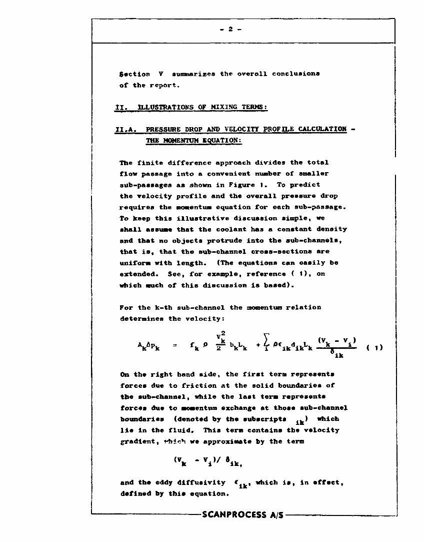
Section V summarizes the overall conclusions
of the report.
II. ILLUSTRATIONS OF MIXING TERMS;
II.A. PRESSURE DROP AND VELOCITY PROFILE CALCULATION
THE MOMENTUM EQUATION:
The finite difference approach divides the total
flow passage into a convenient number of smaller
sub-passages as shown in Figure 1. To predict
the velocity profile and the overall pressure drop
requires the momentum equation for each sub-passage.
To keep this illustrative discussion simple, we
shall assume that the coolant has a constant density
and that no objects protrude into the sub-channels,
that is, that the sub-channel cross-sections are
uniform with length. (The equations can easily be
extended. See, for example, reference ( 1), on
which much of this discussion is based).
For the k-th sub-channel the momentum relation
determines the velocity:
V.2
E b k L k + k ^ i k d i k L k ^ ik
V*k = f k p -r bkLk + 1 *cikdikLk ( \ V i > < i >
On the right hand side, the first term represents
forces due to friction at the solid boundaries of
the sub—channel, while the last term represents
forces due to momentum exchange at those sub-channel
boundaries (denoted by the subscripts ..) which
lie in the fluid. This term contains the velocity
gradient, f*hic*i we approximate by the term
(vk - v ' V and the eddy diffusivity € ., which is, in effect,
defined by this equation.
SCANPROCESS A/S

- 3 -
(The equivalent differential form of the momentum
exchange term is the familar expression
P€ (differential area) ~ , (21) dy
where y indicates the direction normal to the
differential area.)
The last term of equation ( 1) is called the "mixing"
or "interchange" term because it represents inter
actions between the fluid flows in adjacent sub
channels. The main body of this report is concerned
with estimating the size of this term.
Before we begin that subject, however, it will be
helpful to consider another equation in which there
is a mixing term: the energy equation.
II.B. COOLANT TEMPERATURE CALCULATIONS - THE ENERGY
EQUATION:
The total flow passage is imagined to be divided
into a convenient number of sub-channels, as was
the case for the momentum equation. This time,
however, the conservation of energy equation for
the k-th sub-channel pertains:
dt n r-1 /t.. — t. % W*CP * r - \ hkb
Kj (tj - V +1 W i n "8ik
The first term on the right hand side represents
convection of energy in from the solid walls of the
sub-channel. The last term is again a mixing term,
analogous to the mixing term in equation ( t).
(In differential form this term has the form
SCANPROCESS AS

««. (differential area) at ( kv
V * to Sy
where y indicates the direction normal to the
differential area . )
II.C. OTHER DIFFUSION PROBLEMS:
Equation { 1) describes the diffusion of momentum,
while equation ( 3) describes the diffusion of
thermal energy. Similar equations describe the
diffusion of chemical species.
Experiments made to dftermine the rate of mixing,
or the size of the mixing term, are usually made by
injecting SOD«: chemical into the coolant stream
and sampling the coolant stream at downstream sta
tions.
Equations analogous to equation ( 3) then transform
the chemical concentration data into mixing data,
the primary quantity desired being *J]J»
II.P. SOME CONCLUDING REMARKS:
It will be noted that the term (^<ijc occurs in
the mixing terms of both equations ( 1) and ( 3)«
It has the dimensions of a flow rate per unit of
length, kg/sec m. For that reason, it is sometimes
called an "interchannel flow rate" or a "mixing
flow rate" or by some similar designation. But
the term
"«rr • "ik < » > • ik
has the same units and so is also sometimes called
SCANPROCESS A/S

by the some names. Therefore, when data are presented
in terras of such flow rates, it is necessary to check
carefully how the data have been reduced and which
"flow rate" is actually meant.
Three additional considerations deserve passing
notice at this point. First, the difference equations
( l) and (3) characterize the momentum and
energy exchange at an interface by just two regions:
the sub-channel from whence the fluid immediately
comes, and the adjacent sub-channel to which it is
immediately going. Thus the equation claims that
the fluid remains long enough in a given sub
channel to take on the characteristics of that sub
channel completely, and to "forget" all the
characteristics of other channels through which
it has previously passed. In other words, the
formulation emphasizes the diffusiona! aspect of
the transport and neglects any gross convective
effects, for which cases the transport would not
be proportional to the velocity or temperature
gradient. Some of the mixing data available in the
literature show clearly that under some circuastances
this assumption is entirely unjustified. This aspect
will be discussed again in the following sections.
The second consideration concerns the difference
between the eddy diffusivity for momentum, to be
used in the momentum equation, and the eddy diffu
sivity for thermal energy, which is used in the
energy equation, and the eddy diffusivity for
chemical species, the quantity determined by most
experiments. Strictly speaking, although these
quantities are closely related, they are not equal.
Nevertheless, in most situations they do not differ
by very much. In any case, the inaccuracies in
volved in predicting mixing are so great that it is
SCANPROCESS A/S

not worthwhile to worry about any small differences
in this respect.
Third, equations ( f) and ( 3) imply no restric
tions on the mixing flow rates vjjc- F o r fully
developed flow, however, the condition of conserva
tion of mass requires for each sub-channel i that
total mixing _ total mixing flow out of i _ flow into i <
which is to say
y w! K
k ^ ki
for all sub-channels k bordering on i. For all
the data reported here, however, the various data
reduction schemes have all employed the stronger
general condition
'ik " Wk± • ( 7 )
that is, for each interface the mixing outflow
equals the mixing interflow. This assumption may
contribute errors in mixing data, particularly if
cross flows are present.
These three considerations (among others) imply
a certain amount of inaccuracy in the mixing data
presented in the literature. However, most
applications which require mixing data do not
require very accurate data. Frequently adequate
predictions of velocities and pressures in rod
bundles can be made with only crude estim ces of
the eddy diffuslvity. Sometimes only the right
order of magnitude is required.
For these reasons one neither requires nor expects
too much of the experimental data available.
SCANPROCESS A/S

- 7 -
III. MIXING AROUND BARE RODS:
III.A. DATA FROM THE LITERATURE:
References ( 2 - 6 ) present mixing data taken
from bundles of rods without mixing promoters. The
reports give the data in various forms according
to the various purposes for which the data was
taken. For comparison purposes Table 1 displays
all this data reduced to the same form. The table
presents the mixing data as
d, ik
w:, A ik5~7 xk A xk
— w. w.
( 8). i
Equations ( 1) and ( 3) indicate the origins
of this mixing term. The sub-channels denoted by
the index i are shown in figure 1. The symbol
w. denotes the flow rate (mass time ) in a x
sub»channe1. The factor w! is actually defined
by equation ( 8); it is intended to suggest the
rate of mixing flow exchanged between adjacent
sub-channels i and k through one common inter
face of width d. , per unit of length of flow.
Thus w' has the units (mass time" length ), X A
and the mixing variable w' /w has the units * X A X
(length" ). In some reports the authors have omitted some
information which is required to compute the
Reynolds number or to reduce the data to the form
w' /w.. In those cases the missing data have been
assumed. These assumptions are indicated by question
marks (?) in the table, and all computed data affected
by the assumption are similarly marked.
Data neither given nor required are indicated by a
horizontal dash in Table 1.
SCANPROCESS A/S

III.B. A PREDICTING METHOD:
A mere collection of mixing data from the literature
would be mildly interesting but not of great use
fulness. What is needed is some method for pre
dicting the mixing so that predictions can be
compared to the data and some insight gained into
the problem.
Kattchee and Reynolds ( 1) suggest a method for
predicting mixing around bare rods. The method
equates the turbulence eddy diffusivity in the
sub-channel, €. , to that in the center of a ' x
circular tube with a fluid flow at the same Reynolds
number as in the sub-channel:
R ei = Hb^ ( 9). x
where w. is the flow rate in the i-th sub-x
channel, and b. the wetted perimeter of the sub
channel. An empirical formula for the eddy
diffusivity at the centerline of a circular pipe,
given by ( 1) is i SS. \/£ (TO) V = 20 U ' K '
Therefore we estimate € in equations ( l),
( 3), and ( 8) with equation (10):
€ik € . Re . If. X X i l l
V ' 20 V 2 (11)
where we find f. using Re. and empirical data
for circular tubes.
Equations ( 8 ) , ( 9). and (11), when combined,
yield a prediction of the mixing M\^Jyt* °* t n e
form
SCAN PROCESS A/S

- 9 -
I k - 2 2 y dik (ir>) w. " 20 5,,_b, i ik i
which has hppn used to generate the predicted
mixing rates shown in Table 1. These rates are
thus the mixing rates expected from the general
normal turbulence level in the flow along the rod
bundle.
Kattchee and Reynolds ( 1) actually suggest the
use of an average €.. , based on an «. computed
for the i-th sub-channel and an € computed
for the k-th sub-chnnnel, in order to allow for
cases where the i-th and the k-th sub-channels
are not identical. And in fact for most of the
experiments reported here the adjacent sub-channels
are not identical. Ho'-rever, the differences are
small and in any case only a mean velocity over the
entire rod bundle is available for computing the
sub-channel flow rates. Therefore in the predic
tions made by equation (12) the rod lattice was
taken as infinite, with all sub-channels identical.
III.C. COMPARISONS:
Table 1 shows the data and the predictions for
mixing around bare rods. In particular, the last
column shows the ratio of the measured mixing rate
to the mixing rate predicted by equation (12) for
the same geometry end Reynolds number as pertained
to the test. The predictions range from a factor
of 16 too low to a factor of 2 too high.
Furthermore, it is difficult to find a pattern in
the discrepancies between data and predictions.
The situation for the data of references (3» » 5)i
whose experimental situations were roughly similar,
SCANPKOCESS A/5

- 10 -
is very bad, the predictions for these data being
wrong in a very unsystematic way, varying between
factors of 9 and 1.5 too low.
The best pattern seems to appear in a plot of the
ratio of observed to predicted mixing vs. the
predicted mixing, shown in Figure 4. Despite
the scatter in the certer of the plot, there is a
perceptible trend downward to the right. The
greater the mixing is expected to be, then the
greater should be the accuracy of the expectation.
III.D. CONCLUSIONS:
The agreement between data available in the lite
rature and predictions made by the method of Kattchee
and Reynolds ( l), equation ( 9)» is not very
satisfactory. It is not clear, however, whether the
discrepancies between data and predictions are due
to a poor predicting method, or unreliable data,
or both. Figure k indicates, however, that the
data available should not be regarded as very
accurate, a great amount of scatter being plainly
evident.
It is likely that the data in many instances are
unreliable, as many of the experimenters report
that only slight variations in experimental
conditions disturbed the mixing results appreciably.
The effects of rod misalignment and cross-flows
seemed to be especially large. In addition, one
can suggest as a sour •- of error extra turbulence
introduced by the tracer fluid injection and
pick-up system. In addition, it may have happened
that some experimenters located their injection
and pick-up apparatus far enough upstream in the
SCANPROCESS A/S

- TI -
rod bundle so that the velocity profile was still
developing, with bad effects on the data.
Finally, none of the references attempt to estimate
their overall experimental uncertainty. The
reported mixing rates are, after all, computed
quantities. The measured quantities in the mixing
experiments are some kind of chemical concentration
versus length. These are then converted into
mixing rates by a lumped parameter model of the
mixing process. It is quite possible that small
uncertainties in the measured concentrations yield
large uncertainties in the computed mixing rates.
It may also be that the predicting method is not
too satisfactory. It could perhaps be improved by
some attempt to take account of the lumping error, (c - c ) that is, the amount by which k i/6.v departs
from •¥•» , but there is some question whether
this would be desirable i the same is not done
in reducing the raw data to obtain the experimental
mixing rates.
There the matter must rest, without a clear result
other than that it seems likely that the data
available are not reliable.
IV. MIXING AROUND RODS WITH FINS OR WIRE WRAPS:
IV.A. DATA FROM THE LITERATURE;
References (2, 3, 5)« which presented data used
in the previous section, also give mixing data
taken from bundles of rods with fins and wire
wraps. In addition, references (13 - 16) provide
data only from bundles with wire wraps.
SCAMPROCESS A/S

These data, presented in the reports in various
forms, has been reorsanized in the manner described
in Section III for data from bare rods. Table 2
presents the reorganized nixing data, along with
the relevant geometry and flow specifications for
each experiment.
IV.B. PREDICTING METHODS FROM THE LITERATURE:
1. Method of Kattchee and Reynolds ( l).
As in the previous section, a simple tabula
tion of the available data is not very useful.
Again it is necessary to compare the data
to predictions in order to gain insight into
the problem.
One obvious choice of a predicting method is
the method proposed by Kattchee and Reynolds
(1) for bundles of bare rods, as used in
the previous section. It is true that the
method did not seem to work out so well in
that case, but the fault was probably due
more to the data than to the predicting method.
In any case, predictions by this method have
been made for each data point for mixing with
fins or wraps, and these predictions are also
tabulated in Table 2.
2. Method of Collins and France ( 2).
Collins and France ( 2) suggest that w!./w. IK X
should be equal to the ratio of the cross
sectional flow area swept by the fins to the
total cross flow area, divided by the flow
length:
i k w.
1
" •
1 L
A f i A.
i (13)
SCANPROCESS A/S

- 13 -
This suggestion is patently absurd since for
fully established flow the mixing w±\/"±
cannot be a function of the flow length. In
addition, the pitch of the fins, oaitted from
equation it J), obviously will have an important
effect or the magnitude of w' /w. .
Method of Shimagaki and Preede (7 3)
and Waters ( 5 ) .
Both Shimazaki and Preede (13) and Waters ( 5)
suggest that the product of the mixing wJJ(/wi
and the fin or wrap pitch p should be a
constant for a given rod geometry (rod diameter
and rod pitch). This is equivalent to saying
that each revolution of fin or wrap carries
a definite fraction of the total flow with it,
no matter what the pitch is.
Shimazaki and Freede (13) reported only one
data point, and so were unable to evaluate
their suggestion in detail, but the later work
of Waters (5) embraces a series of experiments
on one rod bundle but with various rod pitches.
Waters shows that for his bundle the quantity
w!.p/if. is indeed almost constant over a wide xkr i
range of wrap pitch.
The quantity "ivP/1*"- c a n hardly be a constant
for all mixing situations however. Firstly,
this mixing quantity depends upon the sub-channel
shape chosen for analysis. Secondly, as Waters
( 5) points out, the rod bundle geometry must
have some influence, especially the height
of the fins compared to the diameter of the
rods. Thirdly, we have no special reason to
expect that the same fraction of the total
flow will follow the fins for all Reynolds
SCANPROCESS A/S
Ik -
numbers. Very viscous fluids, for instance,
should show much different nixing characte
ristics than fluids of low viscosity.
These objections notwithstanding, the Shiiaazaki-
Freede-Vaters suggestion remains of interest,
and will be discussed again in a following
section.
IV.C. A NEW SUGGESTED PREDICTION:
1. Predicted mixing rates.
Oddly enough, none of the references discussed
above attempt to begin at the beginning and
predict mixing rates in the simplest way possible,
even though they all hint at such a prediction.
A simple prediction requires only a simple
•odel of the a&ixing process. The following
idealized mixing model will yield a useful
prediction of the mixing rate:
In the model, the mixing comprises two parts:
outward mixing away from the rods and fins
into the centers of the sub-channels, and
"lateral" or "peripheral" mixing around the
rods from sub—channel to sub—channel. In
harmony with the lumped parameter idea, the
first kind of mixing (due to general dis
orderly turbulence) is, in the model, in
finitely large and makes the velocity and tempe
rature in a given sub-channel uniform.
The lateral mixing in the model on the other
hand, derives entirely from the orderly action
of the fins, which sweep along all the fluid
SCANPROCESS A/S

- 15 -
in front of them from sub-channel to »ub-channel
as the main flow proceeds along in the direction
of the axis of the rod bundle.
Thus Figure 2 shows schematically the basic
computational picture. Consideration, for the
moment, of the action of only one wire or fin
will give a picture of the "basic mixing action",
so to speak. What flow rate from sub-channel
i to sub-channel k does this picture imply?
For this model, the mixing rate predicted is,
in words,
flow rate pushed by the wire from i to k per unit axial length
total flow rate in sub-channel i
fraction of the cross sectional area of i which is swept by the wire axial distance required for the helically wrapped wire to pass through the subchannel cross section,
or, in symbols,
w' ( w ^ )
i one wire
(Afi/Ai) ( »p/2ff>
(14).
As equation ilk) may not be self-evident,
the Appendix gives a derivation.
This result for the basic mixing action, although
it oust in some way be related to the actual
mixing, cannot really predict even the idealized
mixing.
In the first place, the model only shows fluid
SCANPROCESS A/S

leaving sub-channel i, whereas the true mixing
idea pictures an equal rate of inflow through
the interface from sub-channel i. Secondly,
in most geometries two wires, each on adjacent
rods, are attempting to sweep fluid through
the same interface. Each, therefore, cannot
be perfectly effective.
How then does the basic mixing calculated
for one wire, equation (l4), relate to
w.'./w. ? ik i
Presumably the mixing situation is too com
plicated to allow a simple pencil-and paper
answer to this question. Therefore, at this
point the "analysis'* ends, and the mixing study
starts the following program:
1. Assume that equation (1*1) gives
the mixing w'/w., and make mixing lk i
predictions on this basis for ex
perimental geometries reported in
the literature.
2. Compare these predictions to the
mixing data reported in the lite
rature.
3« Seek a pattern in the discrepancies
between prediction and experiment;
try to find parameters which correlate
the errors.
The antepenultimate column of Table 2 shows
the predicted mixing rates which result from
steps (1) and (2) above. A comparison,
summarized in the penultimate column, of this
column with the experimental mixing rates shown
SCANPROCESS A/S

- 17 -
in the first of the mixing rate columns, shows
the discrepancies between the simple mixing
predictions and the data.
Section 2. below describes the third and final
step in the program.
2. Correlation of discrepancies between data and
predictions.
a. "Slipping over the fins"
A correlation of the errors requires at
least a modest analysis of the sources of
error. Undoubtedly part of the error comes
from the "slipping" of some of the fluid
over the fins; contrary to the fin
sweeping assumption above, the fins cannot
sweep all the fluid in front of them.
Simple physical reasoning can reveal a
useful correlating variable for this source
of error. Briefly, "slipping" should in
crease with increases in
1. The "axial inertia" of the flow,
describing the tendency of the flow
to persist in the axial direction,
2. the "obliqueness" of the fins across
the axial direction of flow, equal
to D/p,
3. the peripheral spacing between fins
or wires on a "od;
and "slipping" should decrease with in
creases in:
SCANPROCESS A/S

- 18 -
1. the "viscous forces" in the flow,
2. the height of the fins.
A simple combination of these has the form
„ , . . „ ("axial inertia")(D/p)(q) "slippmg" oc (»viscous forces»)(h)
which gives directly the desired correlating
variable
Re " s l i p p i n g " oc (£) #h^ ( 1 5 ) . <S> <$>
Denote this proposed correlating variable
by CV. Then, if the error is evaluated
in terms of
predicted mixing observed mixing
then R should increase with CV. As CV
increases, the slipping over the fins in
creases and the simple prediction of mixing,
based on perfect fin sweeping, should more
and more exceed the actual mixing.
b. Other geometrical effects.
The situation at the interfaces should
contribute other important errors, especially
if two fins or wires try to push fluid
through the same space at the same time.
The errors should depend on whether the
wires or fins are turning in the same
direction through the interface ("confluent")
or in oposite directions ("opposing").
SCANPROCESS AS
- 19 -
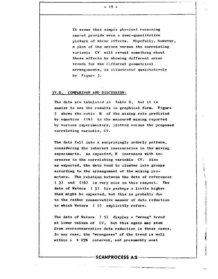
It seems that simple physical reasoning
cannot provide even a semi-quantitative
picture of these effects. Hopefully, however,
a plot of the errors versus the correlating
variable CV will reveal something about
these effects by showing different error
trends for the different geometrical
arrangements, as illustrated qualitatively
by Figure 3-
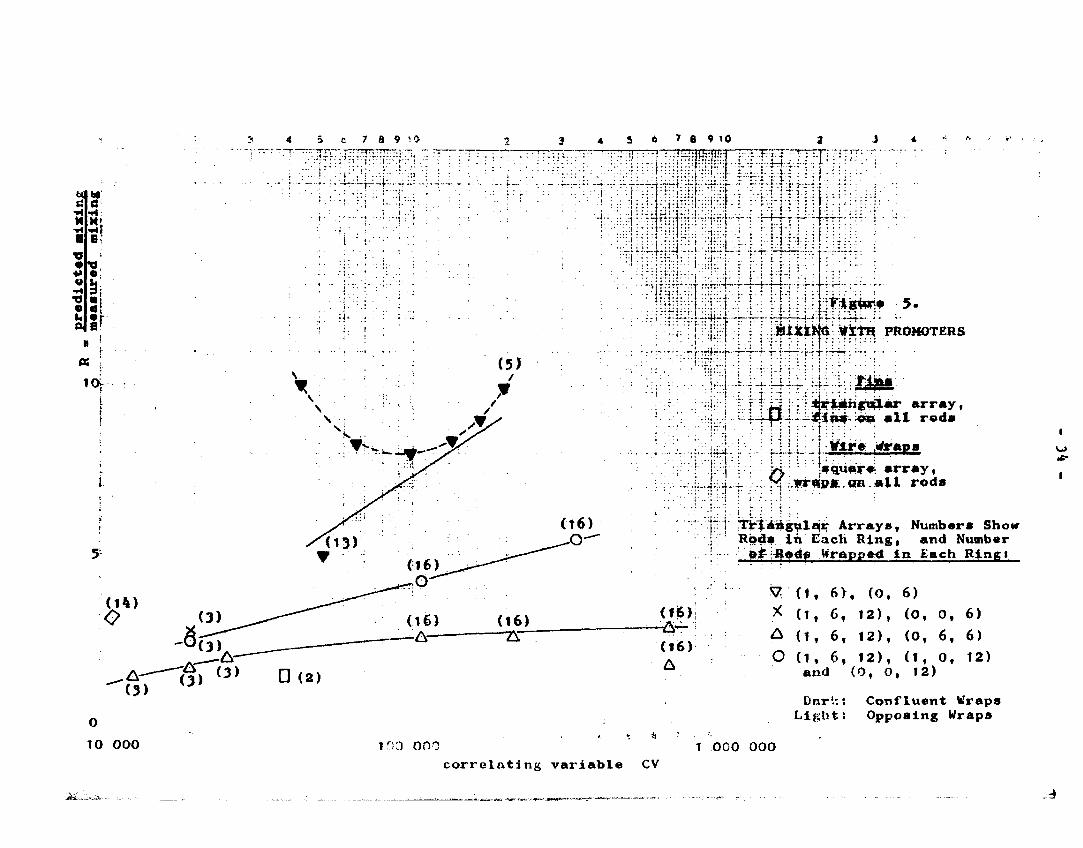
IV.D. COMPARISON AND DISCUSSION:
The data are tabulated in Table 2, but it is
easier to see the results in graphical form. Figure
5 shows the ratio R of the mixing rate predicted
by equation (14) to the measured mixing reported
by various experimenters, plotted versus the proposed
correlating variable, CV.
The data fall into a surprisingly orderly pattern,
considering the inherent inaccuracies in the mixing
experiments. As expected, R increases with in
creases in the correlating variable CV, Also
as expected, the data tend to cluster into groups
according to the arrangement of the mixing pro
moters. The relation between the data of references
( 3) and (l6) is very nice in this respect. The
data of Waters ( 5 ) lie perhaps a little higher
than might be expected, but this is probably due
to the rather conservative manner of data reduction
to which Waters ( 5) explicitly refers.
The data of Waters ( 5) display a "wrong" trend
at lower values of CV, but this again may stem
from overconservative data reduction in these cases.
In any case, the "wrongness" of the trend is well
within a ± 25% interval, and presumably most
SCANPROCESS A/S

- 20 -
mixing experiments ^hov this iruch uncertainty.
Reference il't) provides the only data for a
square lattice, and thus little may be concluded
here.
Reference ( 2) provides the only data for mixing
with fins rather than wire wraps. As might be
expected, the mixing seems greater in this case
than for wire wraps.
Figure 6 shows what is essentially the same nixing
data as is shown in Figure 5» hut this time
organized according to the suggestion of Waters
( 5) and Shimazaki and Freede (13) discussed
in Section IV.B.3 above. The ordinates are the
dimensionless mixing quantities w! p/w . The IK 1
abscissae are the proposed correlating variable
CV discussed in Section IV.C.2 and used in
Figure 5«
Thus Figure 6 is the same as Figure 5 except
that the geometry factor A /A. is missing from
the ordinates. One would therefore expect the
correlations to be worse than in Figure 5, but
in fact the patterns displayed are almost as
satisfactory because for the experiments reported
the range of A /A. was not so large, lying
between about 0.42 and 0.59.
IV.E. CONCLUSIONS:
All considered, the pattern that the data present
in Figure 5 is both orderly and plausible, and
the plot should provide a good basis for estimating
mixing rates for rod bundles with mixing promoters.
The uncertainty is perhaps ± 5094 even for the best
known cases, but it usually is not necessary to
know the mixing rate to a greater accuracy.
SCANPROCESS A;S

- 21 -
The patterns shown in Figure 6 are also good.
This plot offers a more restricted basis for data
correlation, however, as the ratio A„./A., expected
to be important, is not included.
I V. DISCUSSION AND OVERALL CONCLUSIONS: !
} It is evident that the simple diffusive picture
of mixing used by the various experimenters in
reducing their data, and also used in this report
as the basis of mixing predictions, may suffer from
errors from numerous sources. It is entirely
likely that some of these errors are truly major
ones that therefore one can expect neither much
consistency among the data nor good agreement between
data and predictions. j
A consideration of the possible sources of major
error should take into account that:
1 . The basic diffusion assumption that the mixing
rate of any quantity is proportional to the
gradient in concentration does not always
describe what happens in mixing. For mixing
with fins or wraps, the concentration versus
flow length plots of (5) and (13) show
that gross convection effects are considerable.
Even in mixing without fins, the size of the j
turbulent eddies may be so large that the |
mixing process is not primarily diffusive in I
nature. >
2. The mixing flow pattern may not obey the j
symmetry expression ( 7)t i*1 which case the
data reductions of the various experimenters I i
would have no real meaning. j
SCANPflOCESS A/3

- 22 -
3. Extra turbulence introduced by entrance effects,
or by the measuring apparatus, may exceed the
normal turbulene e.
4. Lumping errors may be large, especially for
S/D w 1 .
5. The mixing rate obtained by reduction of
concentration data is rather sensitive to
errors in the raw data.
Considering these sources of possible error, it is
hardly surprising that the data for mixing around
bare rods, summarized in Figure k, seem rather
inconsistent, the ratio of observed to predicted
mixing scattering over almost a whole decade.
Mixing in this case cannot be predicted to within
a factor of 3- This may, however, be good enough,
depending or. the specific application in question.
It is ironic that the data for mixing with fins
and wire wraps, which at first glance seem even
more difficult to measure accurately or to predict,
show a much neater and more understandable pattern
than the data for mixing without mixing promoters.
The available data make as good a pattern as could
be expected, given the uncertainties in the
experiments and the data reduction, and the pattern
is good enough to make some fairly accurate mixing
rate predictions possible. Over the range of the
correlating variable considered, predictions may
perhaps be as accurate as ± 50%.
As a final note, a recurring question concerns
how much the mixing around the rods of a bundle
is improved, over the bare rods case, when fins
or wraps are added. Kattchee and Reynolds ( 1)
SCANPROCESS A/5

- 23 -
suggest an increase by a factor from 2 to 5«
The data comparison in the final column of Table
2 for those cases where experimenters have re
ported data both with and without fins shows that
this suggestion is not far wrong for the systems
studied. The mixing rate without fins, however,
generally exceeds predictions made by the method
of Kattchee and Reynolds ( 1). Therefore it seems
better to predict mixing for wraps or fins in terras
of Figure 5i rather than by using the Kattchee-
Reynolds method to predict the mixing without fins
and then multiplying by a factor of from 2 to 5«
SCANPROCESS A/S

- 2k - ^
ANNOTATED BIBLIOGRAPHY
GENERAL
Kattchee and Reynolds ( 1) provide an overall
introduction to the computation of coolant velocity
and temperature distributions by a finite difference
technique and give discussions of many aspects of
the problem:
1. Kattchee, N., and Reynolds, W.C.: "Hectic
II - An IBM 7090 Fortran Computer Program
for Heat Transfer Analysis of Gas or Liquid
Cooled Reactor Passages,
Aerojet-General Nucleonics, San Ramon,
California, IDO - 28595, December, 1962.
MIXING WITHOUT PROMOTERS
The following references report the data for mixing
around bare rods which are analyzed in Section
III above:
2. Collins, R.D., and France, J.: "Mixing of
Coolant in Channels Between Close-Packed Fuel
Elements",
United Kingdom Atomic Energy Authority, Research
and Development Branch, Capenhurst, IGR - TN/CA
847, January, 1958.
3. Bishop, A.A., et al.; "Thermal and Hydraulic
Design of the CVTR Fuel Assemblies. Topical
Report",
Westinghouse Electric Corp., Atomic Power
Division, Pittsburgh, Pennsylvania, CVNA -
115, June, 1962.
SCANPStOCESS A/S

- 25 -
4. Nelson, P.A., et al.: "Mixing in Flow Parallel
to Rod Bundles Having a Square Lattice",
Westinghouse Electric Corp., Atomic Power
Dept., Pittsburgh, Pennsylvania,
WCAP - 1607, July, i960.
5. Waters, E.D.: "Fluid Mixing Experiments with
a Wire-Wrapped 7-Rod Bundle Fuel Assembly",
General Electric Co., Hanford Atomic Products
Operation, Richland, Washington, HW - 70178,
August 3, 1961.
6. Bell, W.H., and Le Tourneau, B.W.: "Experi
mental Measurements of Nixing in Parallel Flow
Rod Bundles",
Westinghouse Electric Corp., Bettis Plant,
Pittsburgh, Pennsylvania, WAPD - TH - 381,
1958.
There are various reports available which can serve
as supplements to the reports listed above. Bishop,
et al., ( 7 ) is an abstract of work reported in
more detail in ( 3 ) . Reference ( 7) omits im
portant information and has not been used as n c*ita
source. Waters (8) is a newer edition of ( 5),
but contains no new data.
7. Bishop, A.A., et al.: "Coolant Mixing in a
Nineteen-Rod Fuel Assembly",
Transactions of the American Nuclear Society,
Vol. 4, 1961, pp. ky - kk.
SCANPROCESS A/S

8. Waters, E.D.: "Fluid Mixing .Experiments with
a Wire-Wrapped 7-Rod Bundle Fuel Assembly",
General Electric Co., Har.ford Atomic Products
Operation, Richland, Washington, HW -
70178 REV, November, 19^3-
References ( 9) and (10) are predecessors to
reference ( 6). They contain no experimental data,
but only discuss the mixing problem in general
terms:
9. Bohl, H., tt al.: "Mixing Coefficients",
Westinghouse Electric Corp-, Atomic Power
Dept., Pittburgh, Pennsylvania, WAPD - PM - 41,
September, 1955-
10. Griable, R.E., and Bell, V.H. : "An Analysis
of Mixing in Parallel Flow Rod Bundles",
Westinghouse Electric Corp., Westinghouse
Atomic Power Division, WAPD - TH - 178, 1956.
Reference (11) provides a literature survey of
the mixing problem, made by Atomic Energy of Canada
Limited. References listed in that report and which
contain data and which have been released to the
public have been included in the present report.
11. Coates, D.F.: "1 n cer-Ch-.nrel Mixing and Cooling
Temperature Di. *: *.ributir>v \*< Seven and Nineteen
Eltir-nt Fuel Hund ler- - Literature Survey",
Canadian General F.ltctric Co., Ltd.,
Peterborough, Ontario, Canada, AECL - X07 -
10001 R, November, i960.
SCANPROCESS A/S

- 27 -
It is possible that an interesting predicting method
is reported by Zaloudek (12); however, this report
was classified for some time. It has now been
declassified but withdrawn from circulation while
the author is preparing the work for publication.
12. Zaloudek, F.R.: "An Analysis of the Magnitude
of Natural Mixing in the Seven Rod Cluster
Fuel Assembly without Mixing Promoters",
General Electric Co., Hanford Atomic Products
Operation, Richland, Washington, HW - 60376,
May 20, 1959. (Classified).
MIXING WITH PROMOTERS
Mixing data for rod bundles with fins and wire
wraps are given in references ( 2, 3i 5), previously
cited. Shimazaki and Freede (13) and McNown, et el.
(ik) provide additional data.
13. Shimazaki, T.T., and Freede, W.J.: "Heat
Transfer and Hydraulic Characteristics of the
SRE Fuel Element",
Reactor Heat Transfer Conference of 1956,
J.E. Viscardi, Comp., TID - 7529, Part 1,
Book 1, U.S. Atomic Energy Commission, 1957.
14. McNown, J.S., et al.: "Tests on Models of
Nuclear Reactor Elements. II. Studies on
Diffusion",
Engineering Research Institute, University
of Michigan, Ann Arbor, Michigan, AECU - 3757
(Pt. II), March, 1957.
SCANPROCESS A/S

- 28 -
Two reports (15, 16) stemming from Canadian work
provide valuable additional mixing information.
Unfortunately, neither is complete, reference (15)
being a brief journal survey article, and reference
(16) being a rather terse internal report. Between
the two, however, some useful data may be extracted.
15. Lane, A.D., et al.: "The Thermal and Hydraulic
Characteristics of Power Reactor Fuel Bundle
Designs",
The Canadian Journal of Chemical Engineering,
Vol. 41, No. 5, October, 1963, pp. 226 - 23^.
16. Howieson, J.t and McPherson, G.D.: "Coolant
Mixing in 19Element Fuel Bundles",
Atomic Energy of Canada Limited, Nuclear Power
Plant Division, Toronto, Ontario, Canada,
TDSI - 31, July, 1961.
Mensforth and Yonemitsu (1?) describe some interest
ing mixing experiments on wire wrapped bundles, but
the experiments yielded no quantitative results.
17. Mensforth, L.H., and Yonemitsu, I.D.: "Seven
Element Fuel Bundle Flow Studies",
Canadian General Electric Co., Ltd., Civilian
Atomic Power Department, Peterborough, Ontario,
Canada, R 60 CAP 25, June 15t 1960.
SCANPROCESS A/S

- 29 -
A P P E N D I X
DERIVATION OF FIN-SWEEP MIXING PREDICTION
Figure ( 2) shows the control volume for analysis,
seen along the axial direction. The axial flow
through this area is w., and the axial velocity
V is assumed constant over the cross section, even
in the area swept by the fins. (This should be a
reasonable assumption if the fin pitch to rod
diameter ratio is large, as it usually is.) Thus
we have
w å PA.V. (A-1) i i l
The fin sweeping flow per unit of axial length,
w' , upon the assumption that the fins smoothly
sweep forward all the fluid in front of them, is
r o w!, = pw J r dr <A-2) . lk ' r.
i
where OJ is the "rotational velocity" of the fins
through the cross section. We take
2W 21T (A-3). (time for a (p/V±)
full rotation)
Combining equations (A-1), (A-2) and (A-3), we
have r
2ff } r dr w' r .
l k r j 4
w. pA. i i
r ? f r dr
r . i
- U±V2ff) "
( A f i / A i > " (9p/2ff )
(A-4)
where A_. represents t.ie area in the i-th sub
channel which is swept by the fins.
SCANPROCESS AS

- 30
rod diameter D
subchannel i
subchannel i
sub-channel k
Triangular Lattice
subchannel k
Square Lattice
F i g i re 1 .
SUB-CIIANNiiL DLFINITIONS

- 31
sub—channel i (schematic)»
cross-sectioral area A.
F i g u r e 2 .
SCHEMATIC DIAGRAM FOR FIN-SVlii;P
MIXING RATE CALCULATION

V,
o '.: 5* W
«c r:
S > TJ
pr*
O
V -
H
• ^
> 01
5 5 > X n H w a
o o » a n r > H M
« O
< 5 23 r n
o < «
« M H
' . • *
14 X H as o > (0
> "*1
§ o H M O S!
O "»)
X m
o *w
a > H M O
O •n •o w D M
H F3 O
H O
O
R » <; P3 O
c > r M H > H M < r. *o r o s o
n X
O H p: D
H » P» Z O (A
•* H
c i t
*wJ
»
o o 1 1 (D
3 H
<
a o*
o
«>
* 1 1
\
predicted mixing observed mixing
jr lines for
/ different
* _y
wrap arrangements
.f^
etc.
«

•a -
2° a O &
t
O I
1 -'
• D>
S; IT-#,--+*• s s a M
il. • * • !
w •
..-.-*< -
..i .;
; t
• i * » : .10'. .»•!.
«*: *J H«
- i * * - " * " 1 *
O 0 »*
• ' » • • • «
H.
, . a. to --a
o •< 'W
1 measured mix ing 2 p r e d i c t e d mix ing
K •c
< c
«* s P » $ o a t* «•
- n a o. a >* a H- « o ft a »* . ~ . »t o
r - O • - » • • • » • • a > - H ) . **• W j f t .H—
• v . K* JS • • • * " £ • ' • > •
F < » *- o M :«* »
4. £ . : $ . . « . • . * . * c .«. ., . . .
A . ...
S H
H 2 O
* W 1J -S M.
a n rs 3 .*•
o SI »
o 0
I* a a 9 A •»}
a a o
i.
T ;: i . ' .••.
" j •
...j : i ;; 1 . i
i l 1
a
16
• * •
LiHil^-i..
a 9'-
T
o a
15
w
• 'CD -A-
' * 3
-ft' .:r-
IT c n... s * c
OS
o o o
1 * .
- CC -
7 8 9 10 7 8 9 10
bf«*
•bo
•s1
9
u
n
• •
10-
O 10 000 100 000
11 "fe
! »
lip r i - : - ! - .
- t f? '
i!;;:;-.-; :.:t::vj --:
s :
i":
:\Wmn-rkfrf-tttit :-r--r
: i).'
Jaiik^-fcitH PROMOTERS
f a t ,
::!.:.-: - : - f - j ^ * - - - - * $ W- W • array,
i l rod*
; jsquar«; a r r a y , wrajpft tro « H rod«
Tr^Attgular A r r a y s , Numbers Show Rod* i n Each R i n g , and Number ' é#i^t»df Wrapped t n Each Ring:
X
O
( t , 6>, (O, 6) ( 1 , G, 1 2 ) , (O, 0 , 6)
( 1 , 6 , 12 ) , ( 0 , 6, 6) ( 1 , 6 , 12 ) , ( 1 , 0 , 12) and (O, O, 12)
Dnr'.-.i Confluent Wraps Lights Opposing Wraps
1 000 000 correlating variable CV
b 7 8 * 10
3 ;
2 - ~
0.
7?m
fHtP
• ! : f : : ; ; ' •
:;^ •.i-i;;l:"J
m
O (14)
o 10 000
, " t r H',* .•-?[• t^rij
if-it
i?i?:::-T
;,i : : -;...: U-:.... '
j
: j ' .
mi :;;tU..:
4 * 6 7 8 9 .0 2 3 *
MlXtNG WITH PRO^tOTSRB ' . . . . . . . ; : ! .; :..; ij.:..i.i-.;.|4rj-;:.;_i lft«.T..,. . -
D i m e n s i o n i é s s Miking ***-*" p i
Measured, ifleitlt^d Vfi
C o r r e l a t i n g V a ^ i a i l fccV » R * J ;
f- /
9 10 100 000
ti
o
triangular array, Flna on all rods
Wire Wraps square array,
'wraps on all rods
7 e ' io 1 ooo ooo
'Triangular Arrays, Numbers 4hov Hods in Each King, and lftinif«i»r_of Rods Wrapped in , , j: Jiach Ring:
V 1%, 6 ) , (O, 6)
X tit*, 6 , 1 2 ) , ( 0 , 0 , 6)
A.-.^ik-B, 12), (0 , 6, 6) O ii'é 6 , 1 2 ) , ( I , 0 , 12)
a^a ( 0 , 0 , 12)
_. []j^ekth-:t C o n f l u e n t Wraps
• iLligl it: [Opposing Wraps
J i » -
VJI
correlating variable CV
« « * * -*¥-i*'**>5fSr."'"J!?

TABLE 1
DATA FOR MIXING AROUND BAiU. RODS
Reference
Collins and France (2)
Bishop, et al. (3)
Nelson (4)
Waters (3)
Bell and Le Tourneau
(6)
G E O M E T R Y
No.and Array
19 å
19 A
144 sq
7 A
64 sq
Rod Dia. D (in)
3.30
0.500
0.337
0.704
0.333
0.312
Pitch S (in)
3.875
0.600
0.422
0.842
0.375
0.375
u
1 .10
1 .20
1.25
1.196
1.13
1.20
F L O W
Fluid
Air at 1 at.
(?)
Water
Water
Water
Water
Water
Temp .
Room (?)
•*
Room ( ? )
«•
.
*.
Velocity (ft/sec)
» 100
^
11.6
a*
•*
—
He
58000 (?)
37000
30000 (?)
75000
10000 -
30000
10000 -
50000
MIXING HJiSULTS
Observed w' /w. ik 1
x 10 1
50 (in - 1)
(?)
359
113
41 .6
1 1 3
122
Predicted w', /w. J.K 1
4 x 10
3-04
(in"1)
38.6
26.6
27.6
117
187
Ratio:
Observed Predi c ted
16.4
9.30
4.25
1 .50
0.98
0.6",

TA»LI: i
DATA KOFI MIXING AHOUNI) BAJU. I«OUS
Reference
Collins and France (2)
Bishop, et al. (3)
Nelson (4)
Waters (J)
Bell and Le Tourneau
(6)
G t O M L T R Y
No.and A r m s
19 A
19 A
144 sq
7 A
64 sqj
Pod Dia. U (in)
3.30
0.500
0.337
0.704
0.333
0.312
Pitch S (in)
3.875
0.600
0.422
0.842
0.375
0.373
1 .10
1 .20
1.25
1.196
1.13
1.20
K L O «
Fluid
Air at 1 at.
(?)
Water
Water
Water
Water
Wa ter
Tcinp.
Room (?)
„
Room (?)
—
«»
M
V C 1. O C i t V
(ft/sec)
a* J no
_
11.0
—
.
_
I! O
'.ft 000 (V)
3 7000
30000 (7)
73000
1OOOO »
30000
10O00 -
50000
MIXING HbSL'LTS
Observed
Wik / Wi
x 10 *
30 (in-1)
(?)
3:9
1 1 3
'n .6
11"
122
Predicted
wlk / wi
4 x 10
3.o4
(in"1)
38.6
26.6
27.6
1 17
187
Ratio:
Observed Pr *' d i c t e d
16.4
9.30
4.25
1 .50
0.9«
0 . C r, J

TABU 2
DATA row Mixing KITH MIXING PROMOTIRS
I


