WP/06/198
Corruption and Technology-Induced Private Sector Development
Jean-François Ruhashyankiko and Etienne B. Yehoue

© 2006 International Monetary Fund WP/06/198
IMF Working Paper
IMF Institute
Corruption and Technology-Induced Private Sector Development
Prepared by Jean-François Ruhashyankiko and Etienne B. Yehoue1
Authorized for distribution by Roland Daumont
August 2006
Abstract
This Working Paper should not be reported as representing the views of the IMF. The views expressed in this Working Paper are those of the author(s) and do not necessarily represent those of the IMF or IMF policy. Working Papers describe research in progress by the author(s) and are published to elicit comments and to further debate.
This paper asks whether corruption might be the outcome of a lack of outside options for public officials or civil servants. We propose an occupational choice model embedded in an agency framework to address the issue. We show that technology-induced private sector expansion leads to a decline in publicly supplied corruption as it provides outside options to public officials who might otherwise engage in corruption. We provide empirical evidence that strongly shows that technology-induced private sector development is associated with a decline in aggregate corruption. This suggests that the decline in publicly supplied corruptionoutweighs the potential increase in privately supplied corruption that could result from private sector expansion. JEL Classification Numbers: D73, O3, J24 Keywords: Corruption, Occupational choice, Technology, Private Sector Development Author(s) E-Mail Address: [email protected] and [email protected]
1 Jean-Francois Ruhashyankiko is Senior Economic Advisor to the Minister of Finance and Economic Planning of Rwanda. Etienne Yehoue is Economist at the IMF. This paper was initiated while Jean-Francois Ruhashyankiko was Economist at the IMF. We thank Andrew Feltenstein, Senior Advisor at the IMF Institute and Shankha Chakraborty for Comments.
2
Contents Page
I. Introduction ............................................................................................................................3
II. A Simple Model ....................................................................................................................4
III. Empirical Evidence..............................................................................................................9 A. Data Sources and Definitions..................................................................................10 B. Basic Specifications and Preliminary Results.........................................................13 C. Endogeneity, Sensitivity, and Robustness...............................................................15 D. Summary and Discussion of Empirical Results......................................................18
IV. Concluding Remarks .........................................................................................................19
References................................................................................................................................29 Tables 1. Correlation Matrices for Alternative Measures of Private Sector Development, Technology, and Economic Development...............................................................................24 2. Basic Specifications and Preliminary Results......................................................................25 3. Specifications with Instrumental Variables: Tackling Endogeneity....................................26 4. Sub-Panel Sensitivity ...........................................................................................................27 5. Robustness with Dynamic Panel Estimations......................................................................28 Figures 1. Technology Threshold (see Proof of Lemma 2) ..................................................................21 2. Corruption vs. Private Sector Development (Full Panel) ....................................................22 3. Corruption vs. Private Sector Development (3-year Average Sub-Panel) ..........................22 4. Corruption vs. Private Sector Development (5-year Average Sub-Panel) ..........................23 5. Corruption vs. Private Sector Development (Average Cross-Country)...............................23
3
I. INTRODUCTION
Corruption exists in all societies, but is more pervasive in some societies and more common at some time in their evolution. Many scholars have studied why corruption is more widespread in some countries than others. This literature has identified a number of determinants ranging from political modernization (Huntington, 1968), historical and cultural traditions, levels of economic development, political institutions, government policies (Shleifer and Vishny, 1993; Treisman, 2000; and others), to duration in democracy and ethnicity (Ruhashyankiko and Yehoue, 2006).
In this paper, we approach the issue from a different angle. In spite of the lack of disaggregated data on corruption, we propose the first attempt at analyzing corruption at a more disaggregate level, which allows us to propose a new insight leading to new policy recommendations. We ask whether corruption might be the outcome of a lack of opportunities outside politics or the public sector for public officials. In a country with a weak and struggling private sector, it might be easier for an able and ambitious person to accumulate wealth through politics rather than business. Huntington (1968) observes that corruption, like violence, emerges when the lack of opportunities outside politics, and weak political institutions, channels energies into unaccepted norms and behaviors.
We contend that technology-induced private sector expansion is associated with a decline in corruption, as it provides outside options to public officials who might otherwise engage in corruption. Corruption is defined here as the abuse of publicly entrusted power for private ends. Thus, corruption always involves officials from the public sector, and there would be no corruption in the absence of the public sector.
We use aggregate data and combined it with a simple theoretical framework to propose an analysis of corruption at a more disaggregated level. Specifically, we make a crucial distinction between publicly supplied corruption and privately supplied corruption. For publicly supplied corruption, one might think of nepotism, rent seeking by political parties or customs officials, fraud by public accountants, favors to political kingmakers, mismanaged privatization, rigged procurement contracts, and extortions. Part of this type of corruption occurs within the public sector without any interaction with the private sector, while the other part results from the interaction between the public and the private sectors. Concerning privately supplied corruption, one might think of illegal campaign contributions, bribes or gifts. For example, a businessman may offer gifts to public officials in exchange for favorable enforcement of laws and regulations.
We recognize that corruption has a market governed by the law of supply and demand so that analyzing corruption in a framework of supply and demand is not novel. What is unusual, however, is to distinguish two market-segments for corruption—each with its respective supply and demand—and consider their interaction. The first market-segment takes place within the public sector where public officials are at both ends of corruption transactions. For example, a public official may display favoritism and patronage in appointing unqualified close friends or relatives in key positions in the administration. Public officials might also divert part of a public fund into personal accounts. The second market-segment takes place between the public and the private sectors, where each sector can both supply and demand
4
corruption. Thus, the larger the public sector, the greater the opportunities for publicly supplied corruption. Similarly, the larger the private sector, the greater the opportunities for privately-supplied corruption.
We propose an occupational choice model embedded in an agency framework. In the model there are two sectors: public and private. The principal owns the public sector and delegates powers to agents to manage it. Agents face the choice between working in the public sector or the private sector, and may move from the public to the private sector depending on the availability of opportunities. If an agent moves to the private sector, the public sector recruits a new agent in replacement. Agents can be of two types: Risk averse or risk neutral. Risk averse agents dislike any type of risk and as a result will never engage in corruption as corruption involves the risk of being caught. In that sense risk averse agents are considered as honest. Risk neutral agents behave opportunistically. They may or may not engage in corruption depending on the circumstances. In that sense risk neutral agents are considered as opportunistic. Within each group, agents are differentiated by their innate abilities. We show that when the private sector expands due to technology improvement, some agents who might have engaged in corruption will move from the public to the private sector, leading to a decline of the publicly supplied corruption.
Since the private sector expansion is likely to lead to an increase in the privately supplied corruption, investigating which effect dominates becomes an important empirical question. We provide empirical evidence that strongly supports the claim that technology-induced private sector development leads to a decline in aggregate corruption. This, combined with our theoretical analysis, suggests that the decline in publicly supplied corruption outweighs any potential increase in privately supplied corruption that could accompany the private sector expansion. In other words, our analysis—although based on aggregate corruption data—shows that publicly supplied corruption dominates privately supplied corruption.
Our finding calls for increased efforts to collect disaggregated data on corruption, breaking with current reliance on only aggregate corruption data. Although anticorruption strategies should be mindful of tackling both sources of corruption, one should not lose sight of the fact that publicly supplied corruption typically dominates privately supplied corruption. Thus, publicly supplied corruption deserves particular attention. Further, our analysis suggests that anticorruption policies should consider strategies for private sector development. In other words, private sector development appears as a key strategy for fighting corruption.
The paper is organized as follows. The next section lays out the model. Section III presents the empirical analysis. Section IV concludes.
II. A SIMPLE MODEL
In a democratic society power is exercised by the people and for the people. People elect officials who are entrusted with powers delegated to them. Even in a dictatorial society the ultimate owner of public goods are the people. In that sense, every government—regardless of type of political regime—reports, one way or another, to the people. The issue of corruption can then be addressed through an agency framework in which people represent the principal and public officials are the agents. Agents comprise all elected officials as well as
5
all appointees with a position that could allow them to engage in corruption. In other words, agents refer to public officials.
Thus, consider an economy in which people are the benevolent principal and agents are public officials.2 The economy has two sectors—public and private—and M agents. Agents can move from public to private sector if this makes them better off. In case some agents move to the private sector, new agents in the same proportion are recruited so that the number of agents remains constant. The principal entrusts agents with powers to run the country, and to make appropriate economic decisions to provide public goods and services. These decisions span from executive decisions at the highest level of the government down to day-to-day civil servant decisions in the administrative bureaucracy, the police, the healthcare and education systems, etc. In addition, these decisions may also involve agents in state-owned enterprises to encompass the whole public sector.
Agents can be of two types: risk averse with probabilityγ , or risk neutral with probability1 γ− . Risk averse agents dislike any type of risk and as a result will never engage in corruption as corruption involves the risk of being caught. In that sense we also refer to them as honest. In this model, risk averse agents also prefer the public to the private sector regardless of wage differential because the latter involves risk and offers less stability. Risk neutral agents behave opportunistically. They may or may not engage in corruption and may or may not move to the private sector depending on the circumstances. The principal has a probability 0q > of discovering any agent's abuse of entrusted power for personal gains: corruption.
The private sector offers a wage ( ),pw z a , which depends on a technology parameter z and
individual innate abilities a , with ( ), / 0pw z a z∂ ∂ > and ( ), / 0pw z a a∂ ∂ > . This wage is determined by the standard marginal product of labor resulting from profit maximization and such that:
(1) ( )( ) ( ), ( ),
, ,p
A z F K L a Sw z a
L∂
=∂
where ( )A z stands for technology and depends on a parameter z such that ( ) / 0A z z∂ ∂ > .
( ), ( ),F K L a S is a production function with ( )L a being the innate ability-augmented labor,
K a fixed level of capital stock, and S stands for the state of the nature. S can only be of two
2 See Aidt (2003) for an intuitive survey of the literature on corruption that distinguishes the case with a benevolent principal from that with a nonbenevolent principal. In the former case, corruption arises when the benevolent principal delegates decision-making power to a nonbenevolent agent. In the latter case, corruption arises because nonbenevolent government officials introduce inefficient policies in order to extract rents from the private sector. We consider the principal as being the people but distinguish benevolent from nonbenevolent agents. Hence, both these types of corruption can still arise.
6
types, good (G) with probability λ or bad (B) with probability (1 )λ− . If good state of the nature occurs, it yields a private sector wage ( ),G
pw z a . If a bad state of nature occurs , it
yields ( ),Bpw z a with ( ) ( ), ,G B
p pw z a w z a>> . In a simplistic way, one can think of a bad state of nature as being a recession in which economic agents lose their jobs.
Each agent in the public sector earns a wage ( )gw a (with ( ) ( ), ,Bp gw z a w z a<< ), which
depends on individual innate abilities a , with ( ) / 0gw a a∂ ∂ > . In other words, the salary scale in the public sector is driven by innate ability, which we use here in a broader sense to embed the level of education.
Both risk averse (honest) and risk neutral (opportunistic) agents are differentiated by their innate abilities assumed to be distributed in the interval[ ], a a . We assume that an individual with a low innate ability may not be able to work in a high technology environment. In other words, for each technology level zo, there exists an innate ability ao such that only individuals with abilities greater than or equal to ao will be able to work with zo. We refer to these abilities as compatible with technology level zo.
The wedge between public and private sector wages is primarily driven by technology improvement and not innate abilities. Technology improvement could also positively affect the wage rate in the public sector as government would get more fiscal revenue due to technology-induced private sector expansion. But our analysis holds as long as the wage rate increase in the private sector due to technology improvement is higher than that in the public sector.
Among the M public sector agents Mγ are risk averse and will neither engage in corruption nor move to the private sector, while ( )1 Mγ− are risk neutral and hence opportunistic. If an opportunistic agent engages in corruption, we assume that public resources diverted or used for private ends represent a fraction µ of the national incomeY . When corruption is detected—which happens with probability q —we assume that the principal punishes the agent with penalty or fine f . We derive the following result:
LEMMA 1: An opportunistic agent will engage in corruption if and only if:
(2) ( )
.g
Yq qw a Y f
µµ
< =+ +
PROOF:
An opportunistic agent will engage in corruption if and only if his expected payoff from corruption is higher than that from behaving honestly, which is the public sector wage. That is, if:
(3) ( ) ( )( ) ( )1 g gq w a Y qf w aµ− + − >
7
Notice that if corruption is discovered, the agent suffers both a wage loss and the penalty or fine f . The condition above is simply obtained by factoring and isolating q .
When q q> , none of the opportunistic agents chooses to engage in corruption and since honest agents never engage in corruption publicly supplied corruption is null. In addition, privately supplied corruption would also be null in equilibrium since none of the private sector corruptors would find a public counterpart. Hence, this describes a corruption-free economy.
In the remainder of the paper, we make the following assumptions:
ASSUMPTION A1:
,q q< so that all the opportunistic agents behave dishonestly, that is, engage in corruption.
ASSUMPTION A2:
( ) ( ), ,p gw z a w aa a
∂ ∂∂ ∂> that is, the elasticity of the wage rate with respect to innate ability a is
higher in the private sector than in the public sector.
Set [ ] ( ) ( )( )1 gE q w a Y qfµΩ = − + − , the expected payoff from engaging in corruption, and
( ) ( ) ( ) ( ), , 1 ,G Bp p pEw z a w z a w z aλ λ= + − the expected wage from working for the private
sector. Contrary to the wage in private sector, [ ]E Ω is independent of the technology parameter z .
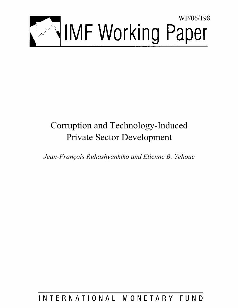
LEMMA 2:
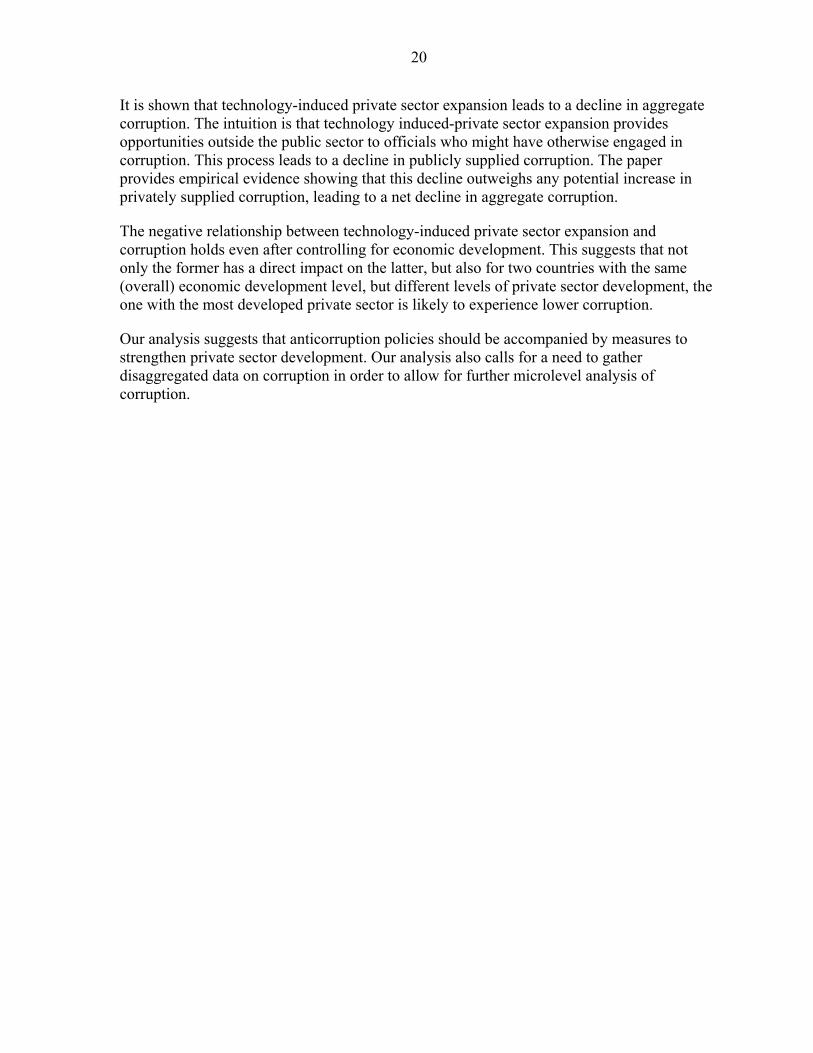
Under A1 and A2, assume [ ], z z z∈ and ( ) [ ]0 z, ,pEw a E< < Ω then, for any [ ], ,a a a∈
there exists a unique ( )z a∗ such that ( ) [ ],pEw z a E= Ω . In addition ( )z a∗ is decreasing in a .
PROOF:
It immediately follows from the monotonicity of ( ),pEw z a in z and assumption A2. In
particular the ( ),pEw z a schedule is upward sloping in z , while the [ ]E Ω schedule is a flat line (see Figure 1). For a given innate ability ( a ) the two curves have a unique crossing point z∗ , since ( )0 z, ( )pEw a E< < Ω . Now, an increase in ( a ) raises the slope of
the ( ),pw z a schedule and shifts the [ ]E Ω line up. However, since ( ) ( ),p gEw z a w aa a
∂ ∂∂ ∂>
and ( )1 1q− < , the move in the ( ),pEw z a schedule is greater in magnitude than the shift in
8
the [ ]E Ω line. As a result, the crossing point z∗ moves to the left leading to a lower technology threshold.
( )z a∗ is the crossing point at which the expected private sector wage ( ),pEw z a , which was
initially lower than the expected payoff of engaging in corruption [ ]E Ω , equalizes the latter and becomes greater as technology improves. It represents the minimum level of technology that would make the wage for an agent of innate ability (a) higher than the expected payoff of engaging in corruption. The monotonicity of ( )z a∗ implies that agents with high innate abilities have lower crossing points. We derive the following result:
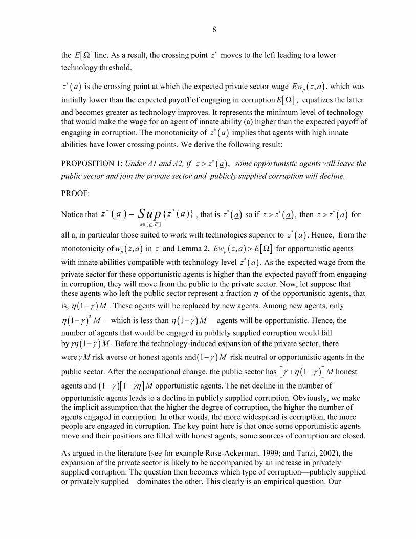
PROPOSITION 1: Under A1 and A2, if ( ) ,z z a∗> some opportunistic agents will leave the public sector and join the private sector and publicly supplied corruption will decline.
PROOF:
Notice that ( ) *
[ , ]
( )a a a
z a z aS u p∗
∈
= , that is ( )*z a so if ( ) ,z z a∗> then ( )z z a∗> for
all a, in particular those suited to work with technologies superior to ( )*z a . Hence, from the
monotonicity of ( ),pw z a in z and Lemma 2, ( ) [ ],pEw z a E> Ω for opportunistic agents
with innate abilities compatible with technology level ( )*z a . As the expected wage from the private sector for these opportunistic agents is higher than the expected payoff from engaging in corruption, they will move from the public to the private sector. Now, let suppose that these agents who left the public sector represent a fraction η of the opportunistic agents, that is, ( )1 Mη γ− . These agents will be replaced by new agents. Among new agents, only
( )21 Mη γ− —which is less than ( )1 Mη γ− —agents will be opportunistic. Hence, the number of agents that would be engaged in publicly supplied corruption would fall by ( )1 Mγη γ− . Before the technology-induced expansion of the private sector, there
were Mγ risk averse or honest agents and ( )1 Mγ− risk neutral or opportunistic agents in the
public sector. After the occupational change, the public sector has ( )1 Mγ η γ+ −⎡ ⎤⎣ ⎦ honest
agents and ( )[ ]1 1 Mγ γη− + opportunistic agents. The net decline in the number of opportunistic agents leads to a decline in publicly supplied corruption. Obviously, we make the implicit assumption that the higher the degree of corruption, the higher the number of agents engaged in corruption. In other words, the more widespread is corruption, the more people are engaged in corruption. The key point here is that once some opportunistic agents move and their positions are filled with honest agents, some sources of corruption are closed.
As argued in the literature (see for example Rose-Ackerman, 1999; and Tanzi, 2002), the expansion of the private sector is likely to be accompanied by an increase in privately supplied corruption. The question then becomes which type of corruption—publicly supplied or privately supplied—dominates the other. This clearly is an empirical question. Our
9
empirical analysis below shows that a technology-induced expansion of private sector leads to a decline in aggregate corruption, suggesting that publicly supplied corruption dominates privately supplied corruption.
Our model shows that corruption might be the outcome of lack of outside opportunities for some public officials or civil servants. The development of the private sector induced by technology improvement provides such outside options, which were previously not available, to public servants. Since there is always a positive probability that anyone engaged in corruption might be caught and fined, outside opportunities, if available, clearly become more attractive. This justifies the migration from the public sector to the private sector once the later offers opportunities.
Beyond the impact of technology-induced private sector development, the usual institutional factors matter as well. In particular, [ ] / 0,E q∂ Ω ∂ < suggesting that institutional improvements, which of course reinforce the probability of being caught, reduce the expected payoff of opportunistic behavior in the public sector. The novelty here is that institutional improvements lower the threshold level ( )z∗ of technology that is compatible with reduction in publicly supplied corruption. In other words, in countries with strong institutions, technology need not to be improved up to the threshold z∗ before the condition
( ) [ ],pw z a E> Ω is met and the countries are able to reduce corruption.
III. EMPIRICAL EVIDENCE
The basic empirical specification to explain aggregate corruption Cit across countries i and over time t can be written as:
(4) C ,it it it t i itZ β δ ν ε= + + + +X γ
where itZ is a variable that captures alternative measures of private sector development; itX is an1 k× vector of exogenous control variables from the existing literature, including economic development; and tδ captures fixed time dummies. i itν ε+ is the error component, where iν denotes the unobservable country specific effect, and itε denotes the remainder disturbance.3 All estimations assume the disturbance has zero mean, the unobservable country specific effect is independent and identically distributed, and both are uncorrelated with the variables itX . The panel covers a sample of up to 127 countries over 1984-2002.
3 Unobservable country specific effects are meant to capture random effects resulting from the use of country point estimates of corruption, drawn from surveys of corruption experiences or perceptions (see corruption data below). Hence, we intend to make inference on the prevalence of aggregate corruption in specific countries.
10
A. Data Sources and Definitions
Corruption Index
There are several sources of corruption data, varying in both country and time coverage. For example, Transparency International (TI) data are only available for the post-1996 period; World Bank (WB) corruption data are available for every other year since 1996. The only corruption data that cover a long time span are prepared by the Political Risk Services group published in the International Country Risk Guide (ICRG), and also available from the World Development Indicators (WDI).4 We use the latter as left-hand side variable.5 Studies that have compared the alternative existing measures of corruption conclude that there is a high correlation among them (Alesina and Weder, 2000; and Treisman, 2000).6 The main reason is that all these sources put together measures of corruption that are based on the same underlying surveys of corruption experiences or perceptions.
Another common feature is that these corruption measures only capture aggregate corruption. Hence, available data do not allow the distinguishing of publicly supplied corruption from privately supplied corruption. Nevertheless, because our model implies that both supplies or sources of corruption work in opposite directions when the private sector expands, the identification of the net effect is a matter for empirical investigation. A positive net effect of private sector development on aggregate corruption would be evidence of the dominance of privately supplied corruption. Instead, a negative net effect of private sector development on aggregate corruption would be evidence of the dominance of publicly supplied corruption.
Private Sector Development Measures
For the size of private sector, we use a number of commonly accepted measures of private sector development. The most widely used measure of private sector development is the domestic credit to the private sector; these data are taken from the WDI.7 Domestic credit to the private sector refers to financial resources provided to the private sector—such as loans, purchases of nonequity securities, trade credits, and other accounts receivables—that establish a claim for repayment. We use domestic credit to the private sector in percent of GDP as one of our measures of private sector development itZ .
4 Notice, the WDI version of ICRG is actually a composite risk measure that consists of subjective scores on five aspects of politics, policy and institutions relevant to the security of property rights in various countries and periods: (i) the political autonomy and expertise of the public bureaucracy; (ii) the degree to which the `rule of law' is institutionalized; (iii) the extent of government corruption; (iv) the risk of expropriation or nationalization of property; and (v) the risk of government repudiation of contracts. 5 The ICRG variable ranges from highest risk 0 to lowest risk 100. Therefore, we use 100 minus the ICRG variable from the WDI. 6 Treisman (2000) noted some inconsistencies with the initial ICRG data on corruption (see footnote 14 p. 409). These do not appear in the WDI version of ICRG that we use. Our sample produces a correlation of 0.73 between CICRG and TI, 0.76 between CICRG and WB, and 0.88 between TI and WB. 7 WDI uses banking surveys from the International Financial Statistics (IFS) and relies on the monetary survey when data are unavailable from the banking survey.
11
Another widely used measure of private sector development consists of some measure of foreign direct investment (FDI). FDI inflows capture the sum of equity capital, reinvested earnings, and other long-term capital from the balance of payments. These inflows, however, tend to capture the general attractiveness of the economy rather than the size of the domestic private sector per se. FDI outward stocks, instead, provide information on the cumulated outflows from the domestic private sector and its success in reaching out to foreign markets. These data come from the United Nation's World Investment Report (WIR). FDI outward stock in percent of GDP is therefore a good alternative measure of private sector development itZ .
Finally, private sector employment data would give a measure of private sector development that fits better the occupational choice framework in our model. Unfortunately, most cross-country sources of employment data do not distinguish between these sectors. Even though manufacturing or industry employment data could be found, it is not possible to disentangle whether the underlying companies are private or government-owned, as in many developing—and even some emerging or developed—countries. Hence, resorting to more aggregate data, we use economy wide labor share in private sector in percent of total labor. This measure is compiled from the International Labor Organization (ILO) and the Organization for Economic Co-operation and Development (OECD). This measure is used in the GMM analysis, which provides a rich set of instruments.
Instrumental Variables
Our investigation of the impact of private sector development on corruption can potentially run into endogeneity problems. Indeed, it is often found that corruption hinders growth and economic development, through its impact on human and physical capital accumulation, FDI, public or private investments (see, for example, Mauro, 1995; Ehrlich and Lui, 1999; Wei, 2000; Tanzi and Davoodi, 2002; and Paldam, 2002). As a result, private sector development might be thought of as the consequence of a decline in corruption. Thus, it is essential to use instrumental variable estimations to produce consistent estimators, and overcome the potential dependence between measures of private sector development and the error terms.
Guided by the insights from our model, technology comes as an obvious candidate for an instrument. Hence, this allows an investigation of technology-induced private sector development on corruption. Technology is captured by total factor productivity (TFP) constructed based on WDI data on real output, real investment, and total employment.8 In order to corroborate the validity of this constructed measure of technology, we also use the number of fixed line and mobile phone subscribers per 1,000 people as a proxy for 8 We make the usual assumptions to construct the panel of TFP variable. First, real investment (constant, 1995 U.S. dollar) is cumulated from 1970 to 1983 in order to determine an initial real capital stock. Second, from 1984 onward (our sample), this initial stock is depreciated at a constant annual rate of 5 percent and augmented by contemporaneous real investments. Finally, TFP is measured as the difference between the natural logarithm of real output per worker and one-third of the natural logarithm of real capital stock per worker, in a Cobb-Douglas fashion with a one-third capital share constant over time and equal across countries.
12
technology. This variable is available from WDI for a large number of countries over the relevant period. Other measures of technology used as instruments include research and development (R&D) expenditures in percent of GDP, and patent applications by residents and nonresidents in thousand. Both variables are taken from the WDI but are only available for a few years from 1995 to 2001. Hence, we use the average for these years as an approximation of the average level of technology over 1984–2002 for each country.
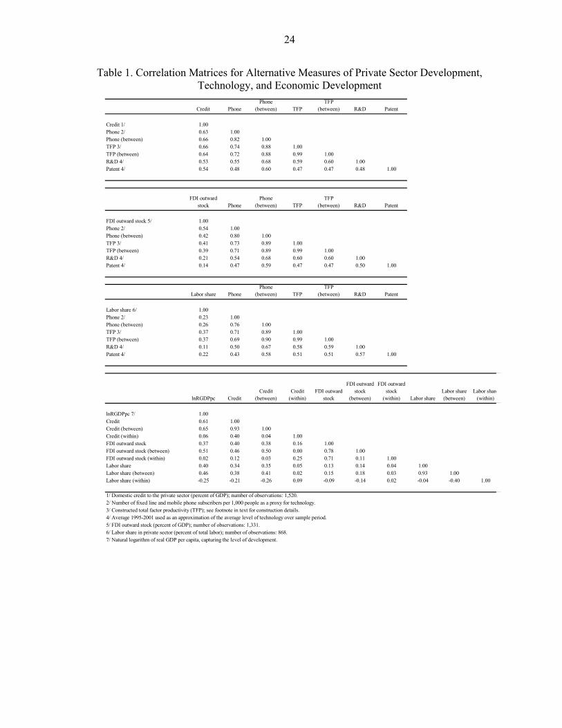
Table 1 presents correlation matrices for our three alternative measures of private sector development, the technology instruments, and the variable capturing economic development. Instruments must be uncorrelated with the error term, and highly correlated with the regressor for which they are to serve as instruments. Our measures of technology appear as reasonably good candidates to instrument domestic credit to the private sector and, to a lesser extent, FDI outward stocks. They appear less appropriate for the labor share in private sector; GMM specifications will allow further instruments for this measure of private sector development.
Control Variables
Treisman (2000) provides one of the most comprehensive cross-country studies of the causes of corruption and finds support for six arguments. Countries with Protestant traditions, histories of British rule, more developed economies, and (probably) higher imports were less corrupt. Federal states were more corrupt. While the current degree of democracy was not significant, long exposure to democracy predicted lower corruption. Ruhashyankiko and Yehoue (2006) provide evidence that, through ethnic fractionalization, early stage of democratization negatively affect corruption in a sample of sub-Saharan Africa. Therefore, these variables provide a useful list of control variables for the determination of the impact of private sector development on corruption.
Data on economic development, captured by the natural logarithm of real GDP per capita, and imports in percentage of GDP are taken from the WDI. Variables for Protestant traditions and ethnic fractionalization come from cross-country data by Alesina and others (2003).9 British rule is a dummy variable for former British colonies. Federal states are captured by a dummy variable. In addition, we introduce government final consumption expenditure in percent of GDP as a variable that controls for the size of government. Finally, time dummies control for time-specific events that are unrelated with these seven control variables.
We are interested in the impact of private sector development on corruption, controlling for all known determinants of corruption. Among these seven control variables, three are time-variant (i.e., real GDP per capita, imports, and government size), and four are time-invariant (i.e., British, Protestant, Federal, and Ethnic); and among the latter two are dummy variables
9 The variable Protestant includes ‘Protestants’ strictly speaking, non-Catholic ‘Christians’ in the Protestant tradition as well as ‘Anglicans’.
13
(i.e., British and Federal). The vector itX for the control variables is also decomposed into two components: the time-variant component 1itX , and the time-invariant component 2 ;iX that is [ ]1 2it it i=X X X .
B. Basic Specifications and Preliminary Results
Recent empirical studies on the determinants of corruption use ordinary, weighted, or generalized least squares (see Treisman, 2000; and Ruhashyankiko and Yehoue, 2006). It is therefore useful to start from such specifications by assuming, for the time being, that all right-hand side variables are exogenous and set 0iν = in our specification (4). These assumptions will definitely be relaxed to allow for other specifications with instrumentation, sensitivity and robustness checks, and more precise account of error components.
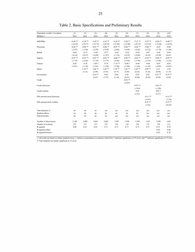
Preliminary results are presented in Table 2. All results are based on robust standard errors. As is common in the literature, economic development comes with a very significant negative sign indicating that developing countries have more corruption. As in Treisman (2000) countries with Protestant traditions have lower corruption. As in Ruhashyankiko and Yehoue (2006) countries with ethnically fractionalized population have more corruption. Consistently with our model, our investigation of the impact of private sector development on corruption needs to control for the size of the government, which we introduce in Column (3). Time dummies introduced in Column (4) capture yearly idiosyncratic shocks that are unrelated with the variables of interest. Column (5) starts removing multivariate outliers using Hadi procedure (see Hadi, 1992, 1994), which will be used systematically whenever possible.
Next, we introduce one measure of private sector development in Column (6). The coefficient on credit is strongly negatively significant giving preliminary indication that a greater private sector development induces less aggregate corruption. This result holds even after controlling for all known determinants of corruption, including economic development. Due to the high correlation of 0.61 between private sector development (e.g., credit) and economic development, our specifications—which always control for economic development—implicitly put a strong requirement on the data. Indeed, we are in presence of multicollinearity, which typically widens the confidence intervals of the regression coefficients and increases the likelihood of type II errors.10 If, notwithstanding the larger standard errors, we still find significant results for private sector development, then we would have identified that private sector development directly affects corruption, independently of its impact on corruption through the general economic development channel.
10 As is well known, a type II error (i.e., fail to reject the null when it is actually significant) is only an error in the sense that an opportunity to reject the null hypothesis correctly could be lost. It is not an error in the sense that an incorrect conclusion was drawn since no conclusion is drawn when the null hypothesis is not rejected.
14
Finding a direct impact of private sector development on corruption is of high importance because the literature so far has shown that economic development is associated with lower corruption. This means that for two countries with different economic development levels, the one with the greater economic development level will experience lower corruption. In other words, two countries with the same overall economic development level should experience the same level of corruption. The finding in this paper suggests otherwise. The significant and negative impact of private sector development on corruption after controlling for economic development suggests that for two countries with the same overall economic development level, but different levels of development (or sizes) for the private sector, the one with the most developed private sector is likely to experience lower corruption.
In order to further ascertain the way in which private sector development directly affects corruption, we complement the basic specification with a transformation of our variable of interest, the private sector development ( Zit ).11 Specifically, we consider whether changes in the average value of private sector development for a country (i.e., between transformation), 1
1.i
i
Tti itTZ Z== ∑ , has a different effect from the temporary departure from that
average (i.e., within transformation), .it iZ Z− , where iT is the total number of time-observations per country. Hence, the basic specification can also be written as:
(5) ( ). 1 . 2C ,it i it i it t i itZ Z Zβ β δ ν ε= + − + + + +X γ
where we still assume, for the time being, that itX is exogenous and 0iν = . Column (7) displays the results. It shows that aggregate corruption appears to be negatively related to the average level of private sector development but positively related to temporary departure from the average. Since the former effect is qualitatively and quantitatively stronger than the latter, the overall effect is negative, as found in the previous Column (6). This result is confirmed in Column (8), which uses FDI outward stock (rather than credit used so far) as an alternative measure of private sector development.
Therefore, the result appears to be driven by cross-sectional (or between) variations in private sector development, rather than time-series (or within) variations. Indeed, cross-sectional variance is much larger than time-series variance. The positive sign obtained for the within estimation might be justified by the fact that it takes time for aggregate corruption to fall in response to private sector development.
This important insight is confirmed in Columns (9) and (10) which replicate (7) and (8) respectively, by relaxing the 0iν = assumption and using random-effects GLS specifications; this assumes zero correlation between iν and itX . Besides few changes among control variables, the results are broadly similar and corroborate our preliminary results. Therefore,
11 For details for such a transformation, see, for example Baltagi (2001), p. 18.
15
country-specific unobservable characteristics—that are not already accounted for by the time-variant control variables 1itX , or time-invariant control variables 2iX —do not appear to have a significant influence on the impact on private sector development on corruption.
C. Endogeneity, Sensitivity, and Robustness
Obviously, our preliminary results are subject to endogeneity problems. We now use a number of methods to check whether our contention that technology-induced private sector development is consistently and robustly associated with a decline in aggregate corruption.
Tackling Endogeneity
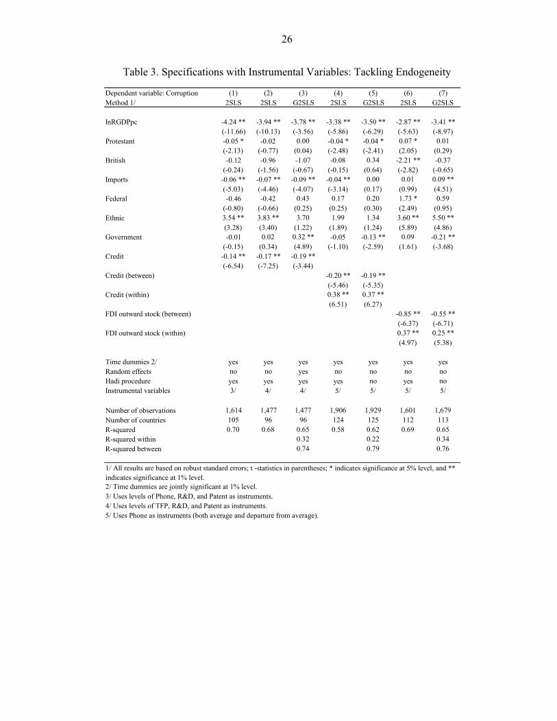
Table 3 reproduces preliminary results from Table 2, but uses instrumental variables. As before, all results are based on robust standard errors. Column (1) uses levels of phone, R&D, and patent as instruments for private sector development; and Column (2) uses levels of TFP, R&D, and patent. Column (3) reproduces Column (2) by using G2SLS—rather than 2SLS—in order to capture potentially unaccounted country-specific unobservable characteristics. On the whole, alternative specifications under these different sets of technology instruments produce consistent results. Aggregate corruption falls as the private sector develops under the impetus of technological improvements, consistently with the contention of our model.
As before, we analyze whether changes in the average value of private sector development for a country .iZ has a different effect from the temporary departure from that average .it iZ Z− . Columns (4) and (5), with credit as measure of private sector development, and Columns (6) and (7), with FDI outward stock as an alternative measure, confirm our basic insight. Not only does technology-induced private sector development reduce corruption, but the impact is not due to temporary departures from the average within countries. Actually, Columns (4) to (7) show that such temporary departures may actually increase corruption. The joint impact, however, is significant and negative (see columns (1), (2), and (3)).
Among the control variables, economic development systematically comes out with a significant negative sign. Thus, even after controlling for economic development, private sector development has a significant and negative impact on corruption. This shows that private sector development directly affects corruption, independently of its impact on corruption through the general level of development channel. This yields strong support to our main finding that technology-induced private sector development is directly associated with a significant decline in aggregate corruption.
16
Subpanels’ Sensitivity
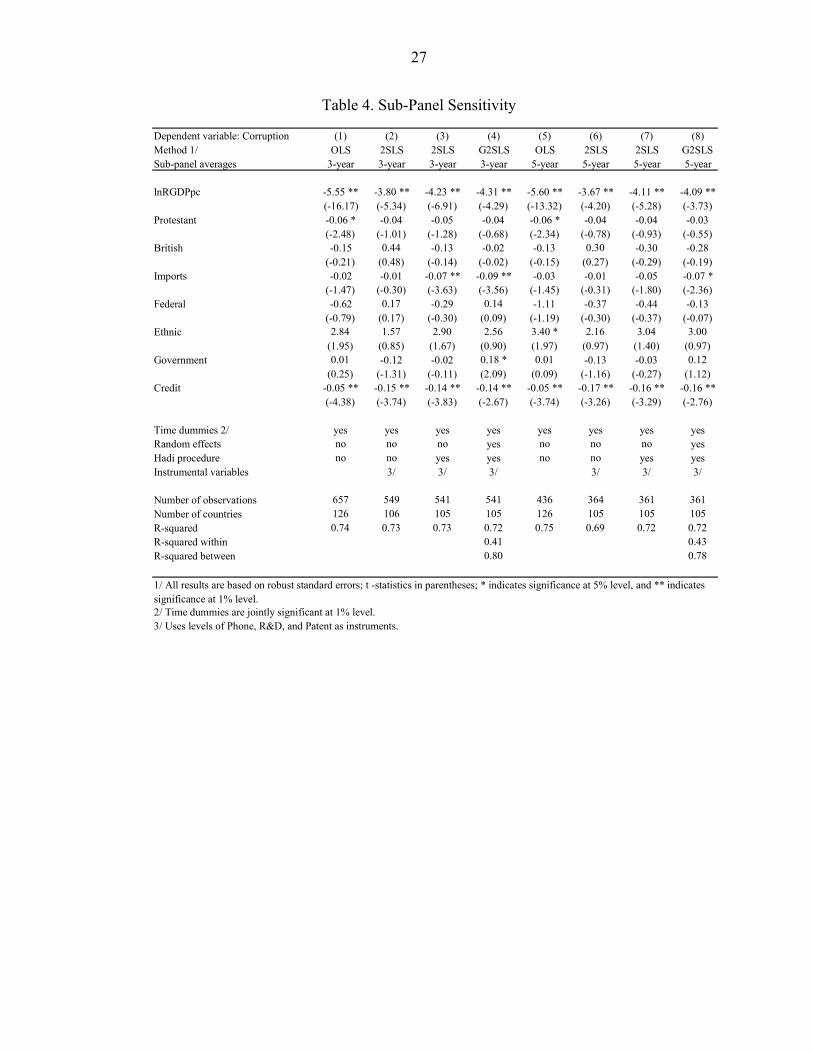
Table 4 reproduces key results from Tables 2 and 3 by collapsing our full panel database into 3-year averages and 5-year averages. We use credit as measure of private sector development, and levels of phone, R&D, and patent as instruments for private sector for the 2SLS and G2SLS regressions.12 Such time-averaging is often performed to remove noise that typically contaminate yearly data. Actually, similar concerns guided our introduction of time dummies in all specifications using our full panel database. Hence, time-averaged results allow evaluating whether our results are sensitive to temporary departures from a steady state, which are partially purged from time-averaged subpanels.
We have already established that our results primarily stem from between effects (i.e., average differences across countries) rather than within effects (i.e., temporary differences from the average within countries). The potential important changes could result from the use of the Hadi procedure to remove multivariate outliers. Because this procedure removes only a small proportion of observations in our full panel, it does not have any significant impact on the results. The use of time-averaged subpanels reduces our sample size and, therefore, outliers identified by the Hadi procedure and heteroskedasticity could, potentially, have a greater impact on our results. The evidence shows this concern is unjustified.
First, Columns (1)-(4) show that the result is not sensitive to 3-year averages whether Hadi outliers are included or not, and whether we use OLS, 2SLS, and G2SLS.13 This 3-year averages subsample covers 126 countries with an average of 5.2 periods, thus about 657 observations. When technology instruments are used, the estimated direct impact of private sector development on corruption quantitatively remains as strong. Thus, estimates from this subsample confirm that, holding economic development constant, technology-induced private sector development is directly associated with a significant decline in aggregate corruption.
Next, this sensitivity analysis is reproduced in Columns (5)-(8) using 5-year averages.14 This 5-year averages subsample also covers 126 countries with now an average of 3.5periods, thus about 436 observations. The same results emerge from this subsample: holding economic development constant, technology-induced private sector development is directly associated with a significant decline in aggregate corruption.
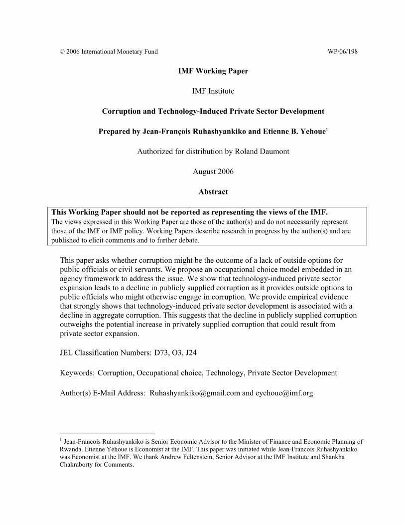
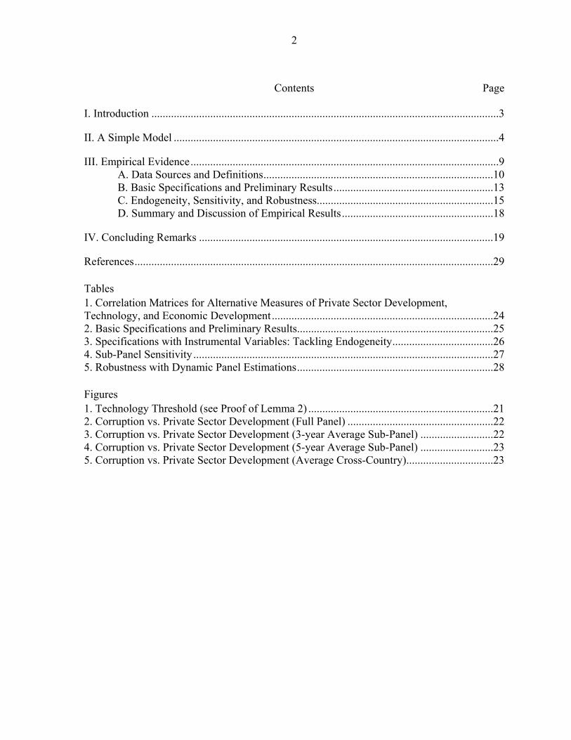
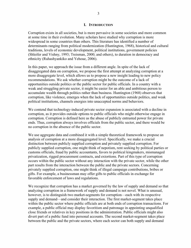
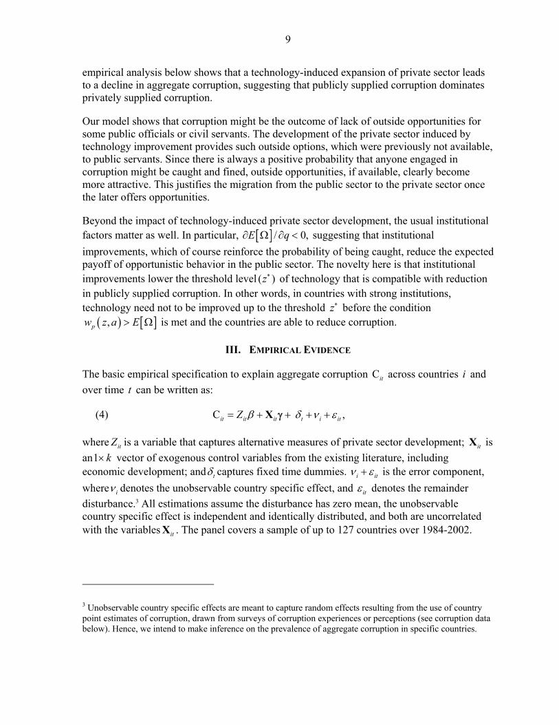
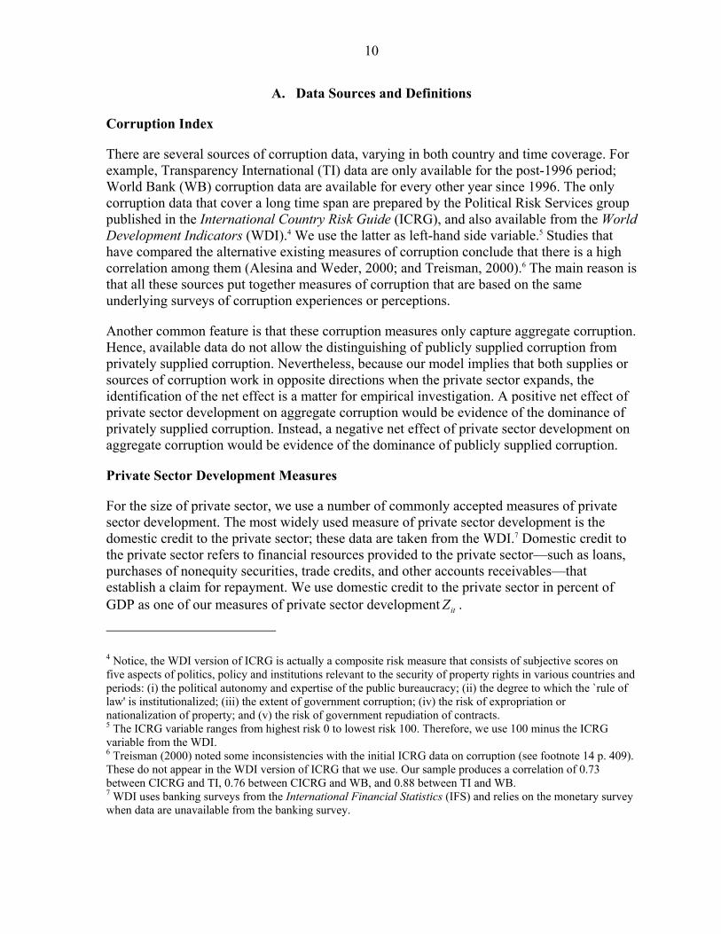
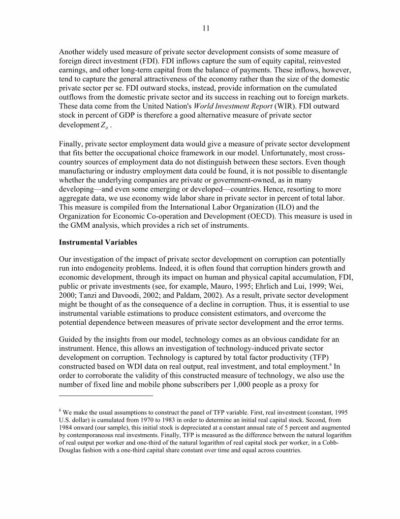
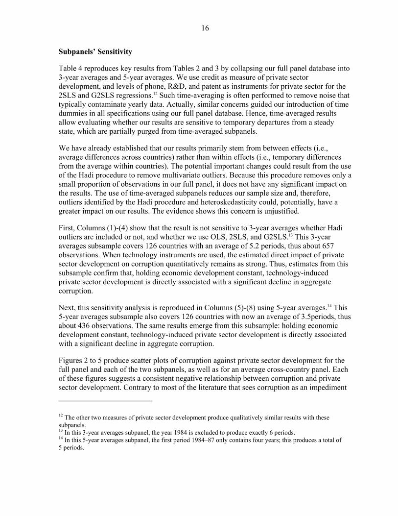
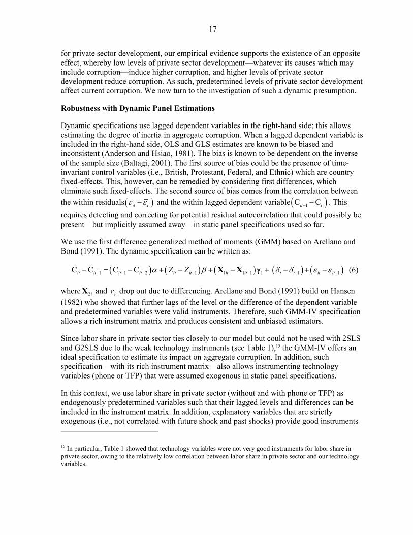
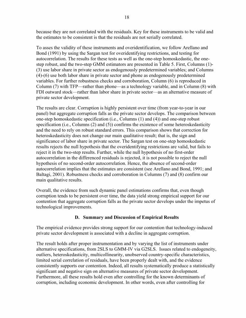
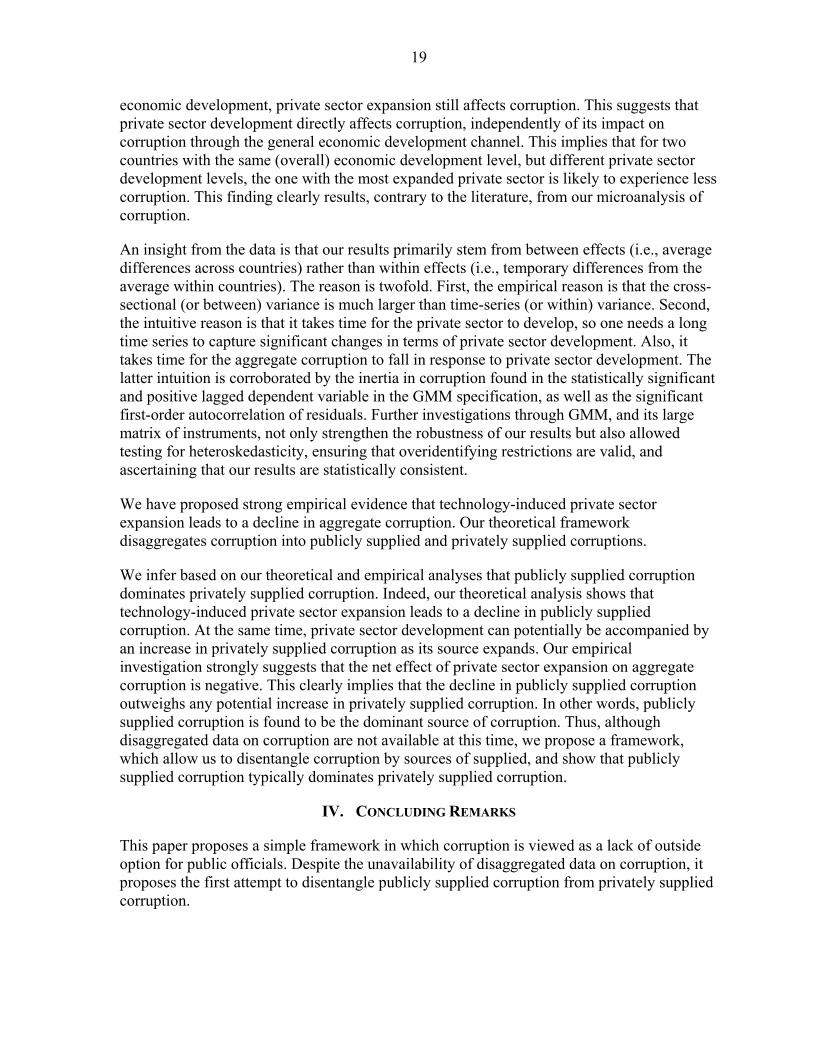
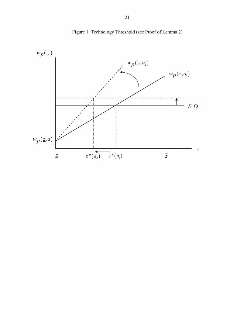
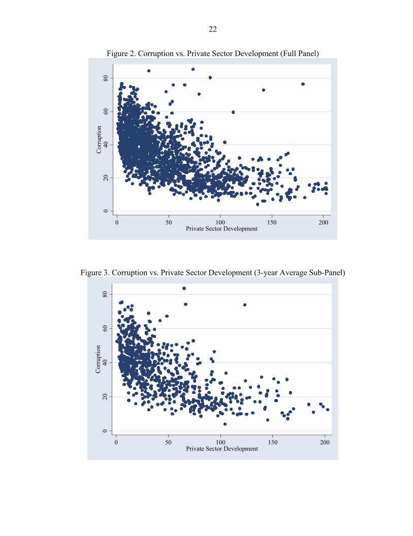
Figures 2 to 5 produce scatter plots of corruption against private sector development for the full panel and each of the two subpanels, as well as for an average cross-country panel. Each of these figures suggests a consistent negative relationship between corruption and private sector development. Contrary to most of the literature that sees corruption as an impediment
12 The other two measures of private sector development produce qualitatively similar results with these subpanels. 13 In this 3-year averages subpanel, the year 1984 is excluded to produce exactly 6 periods. 14 In this 5-year averages subpanel, the first period 1984–87 only contains four years; this produces a total of 5 periods.
17
for private sector development, our empirical evidence supports the existence of an opposite effect, whereby low levels of private sector development—whatever its causes which may include corruption—induce higher corruption, and higher levels of private sector development reduce corruption. As such, predetermined levels of private sector development affect current corruption. We now turn to the investigation of such a dynamic presumption.
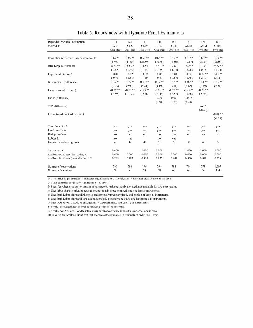
Robustness with Dynamic Panel Estimations
Dynamic specifications use lagged dependent variables in the right-hand side; this allows estimating the degree of inertia in aggregate corruption. When a lagged dependent variable is included in the right-hand side, OLS and GLS estimates are known to be biased and inconsistent (Anderson and Hsiao, 1981). The bias is known to be dependent on the inverse of the sample size (Baltagi, 2001). The first source of bias could be the presence of time-invariant control variables (i.e., British, Protestant, Federal, and Ethnic) which are country fixed-effects. This, however, can be remedied by considering first differences, which eliminate such fixed-effects. The second source of bias comes from the correlation between the within residuals ( ).it iε ε− and the within lagged dependent variable ( )1 .C Cit i− − . This requires detecting and correcting for potential residual autocorrelation that could possibly be present—but implicitly assumed away—in static panel specifications used so far.
We use the first difference generalized method of moments (GMM) based on Arellano and Bond (1991). The dynamic specification can be written as:
( ) ( ) ( ) ( ) ( )1 1 2 1 1 1 1 1 1 1C C C Cit it it it it it it it t t it itZ Zα β δ δ ε ε− − − − − − −− = − + − + − + − + −X X γ (6)
where 2iX and iν drop out due to differencing. Arellano and Bond (1991) build on Hansen (1982) who showed that further lags of the level or the difference of the dependent variable and predetermined variables were valid instruments. Therefore, such GMM-IV specification allows a rich instrument matrix and produces consistent and unbiased estimators.
Since labor share in private sector ties closely to our model but could not be used with 2SLS and G2SLS due to the weak technology instruments (see Table 1),15 the GMM-IV offers an ideal specification to estimate its impact on aggregate corruption. In addition, such specification—with its rich instrument matrix—also allows instrumenting technology variables (phone or TFP) that were assumed exogenous in static panel specifications.
In this context, we use labor share in private sector (without and with phone or TFP) as endogenously predetermined variables such that their lagged levels and differences can be included in the instrument matrix. In addition, explanatory variables that are strictly exogenous (i.e., not correlated with future shock and past shocks) provide good instruments 15 In particular, Table 1 showed that technology variables were not very good instruments for labor share in private sector, owing to the relatively low correlation between labor share in private sector and our technology variables.
18
because they are not correlated with the residuals. Key for these instruments to be valid and the estimates to be consistent is that the residuals are not serially correlated.
To asses the validity of these instruments and overidentification, we follow Arellano and Bond (1991) by using the Sargan test for overidentifying restrictions, and testing for autocorrelation. The results for these tests as well as the one-step homoskedastic, the one-step robust, and the two-step GMM estimators are presented in Table 5. First, Columns (1)-(3) use labor share in private sector as endogenously predetermined variables; and Columns (4)-(6) use both labor share in private sector and phone as endogenously predetermined variables. For further robustness checks and corroboration, Column (6) is reproduced in Column (7) with TFP—rather than phone—as a technology variable, and in Column (8) with FDI outward stock—rather than labor share in private sector—as an alternative measure of private sector development.
The results are clear. Corruption is highly persistent over time (from year-to-year in our panel) but aggregate corruption falls as the private sector develops. The comparison between one-step homoskedastic specification (i.e., Columns (1) and (4)) and one-step robust specification (i.e., Columns (2) and (5)) confirms the existence of some heteroskedasticity and the need to rely on robust standard errors. This comparison shows that correction for heteroskedasticity does not change our main qualitative result; that is, the sign and significance of labor share in private sector. The Sargan test on one-step homoskedastic results rejects the null hypothesis that the overidentifying restrictions are valid, but fails to reject it in the two-step results. Further, while the null hypothesis of no first-order autocorrelation in the differenced residuals is rejected, it is not possible to reject the null hypothesis of no second-order autocorrelation. Hence, the absence of second-order autocorrelation implies that the estimates are consistent (see Arellano and Bond, 1991; and Baltagi, 2001). Robustness checks and corroboration in Columns (7) and (8) confirm our main qualitative results.
Overall, the evidence from such dynamic panel estimations confirms that, even though corruption tends to be persistent over time, the data yield strong empirical support for our contention that aggregate corruption falls as the private sector develops under the impetus of technological improvements.
D. Summary and Discussion of Empirical Results
The empirical evidence provides strong support for our contention that technology-induced private sector development is associated with a decline in aggregate corruption.
The result holds after proper instrumentation and by varying the list of instruments under alternative specifications, from 2SLS to GMM-IV via G2SLS. Issues related to endogeneity, outliers, heteroskedasticity, multicollinearity, unobserved country-specific characteristics, limited serial correlation of residuals, have been properly dealt with, and the evidence consistently supports our contention. Indeed, all results systematically produce a statistically significant and negative sign on alternative measures of private sector development. Furthermore, all these results hold even after controlling for the known determinants of corruption, including economic development. In other words, even after controlling for
19
economic development, private sector expansion still affects corruption. This suggests that private sector development directly affects corruption, independently of its impact on corruption through the general economic development channel. This implies that for two countries with the same (overall) economic development level, but different private sector development levels, the one with the most expanded private sector is likely to experience less corruption. This finding clearly results, contrary to the literature, from our microanalysis of corruption.
An insight from the data is that our results primarily stem from between effects (i.e., average differences across countries) rather than within effects (i.e., temporary differences from the average within countries). The reason is twofold. First, the empirical reason is that the cross-sectional (or between) variance is much larger than time-series (or within) variance. Second, the intuitive reason is that it takes time for the private sector to develop, so one needs a long time series to capture significant changes in terms of private sector development. Also, it takes time for the aggregate corruption to fall in response to private sector development. The latter intuition is corroborated by the inertia in corruption found in the statistically significant and positive lagged dependent variable in the GMM specification, as well as the significant first-order autocorrelation of residuals. Further investigations through GMM, and its large matrix of instruments, not only strengthen the robustness of our results but also allowed testing for heteroskedasticity, ensuring that overidentifying restrictions are valid, and ascertaining that our results are statistically consistent.
We have proposed strong empirical evidence that technology-induced private sector expansion leads to a decline in aggregate corruption. Our theoretical framework disaggregates corruption into publicly supplied and privately supplied corruptions.
We infer based on our theoretical and empirical analyses that publicly supplied corruption dominates privately supplied corruption. Indeed, our theoretical analysis shows that technology-induced private sector expansion leads to a decline in publicly supplied corruption. At the same time, private sector development can potentially be accompanied by an increase in privately supplied corruption as its source expands. Our empirical investigation strongly suggests that the net effect of private sector expansion on aggregate corruption is negative. This clearly implies that the decline in publicly supplied corruption outweighs any potential increase in privately supplied corruption. In other words, publicly supplied corruption is found to be the dominant source of corruption. Thus, although disaggregated data on corruption are not available at this time, we propose a framework, which allow us to disentangle corruption by sources of supplied, and show that publicly supplied corruption typically dominates privately supplied corruption.
IV. CONCLUDING REMARKS
This paper proposes a simple framework in which corruption is viewed as a lack of outside option for public officials. Despite the unavailability of disaggregated data on corruption, it proposes the first attempt to disentangle publicly supplied corruption from privately supplied corruption.
20
It is shown that technology-induced private sector expansion leads to a decline in aggregate corruption. The intuition is that technology induced-private sector expansion provides opportunities outside the public sector to officials who might have otherwise engaged in corruption. This process leads to a decline in publicly supplied corruption. The paper provides empirical evidence showing that this decline outweighs any potential increase in privately supplied corruption, leading to a net decline in aggregate corruption.
The negative relationship between technology-induced private sector expansion and corruption holds even after controlling for economic development. This suggests that not only the former has a direct impact on the latter, but also for two countries with the same (overall) economic development level, but different levels of private sector development, the one with the most developed private sector is likely to experience lower corruption.
Our analysis suggests that anticorruption policies should be accompanied by measures to strengthen private sector development. Our analysis also calls for a need to gather disaggregated data on corruption in order to allow for further microlevel analysis of corruption.
21
Figure 1. Technology Threshold (see Proof of Lemma 2)
E ⎡ ⎤⎣ ⎦Ω
( )1,w z ap
z( )1* az z z( )2* az
( )2,w z ap
( ),w z ap
(.,.)wp
22
Figure 2. Corruption vs. Private Sector Development (Full Panel)
020
4060
80C
orru
ptio
n
0 50 100 150 200Private Sector Development
Figure 3. Corruption vs. Private Sector Development (3-year Average Sub-Panel)
020
4060
80C
orru
ptio
n
0 50 100 150 200Private Sector Development
Figure 4. Corruption vs. Private Sector Development (5-year Average Sub-Panel)
020
4060
80C
orru
ptio
n
0 50 100 150 200Private Sector Development
Figure 5. Corruption vs. Private Sector Development (Average Cross-Country)
020
4060
80C
orru
ptio
n
0 50 100 150 200Private Sector Development
23
24
Table 1. Correlation Matrices for Alternative Measures of Private Sector Development, Technology, and Economic Development
Credit PhonePhone
(between) TFPTFP
(between) R&D Patent
Credit 1/ 1.00Phone 2/ 0.63 1.00Phone (between) 0.66 0.82 1.00TFP 3/ 0.66 0.74 0.88 1.00TFP (between) 0.64 0.72 0.88 0.99 1.00R&D 4/ 0.53 0.55 0.68 0.59 0.60 1.00Patent 4/ 0.54 0.48 0.60 0.47 0.47 0.48 1.00
FDI outward stock Phone
Phone (between) TFP
TFP (between) R&D Patent
FDI outward stock 5/ 1.00Phone 2/ 0.54 1.00Phone (between) 0.42 0.80 1.00TFP 3/ 0.41 0.73 0.89 1.00TFP (between) 0.39 0.71 0.89 0.99 1.00R&D 4/ 0.21 0.54 0.68 0.60 0.60 1.00Patent 4/ 0.14 0.47 0.59 0.47 0.47 0.50 1.00
Labor share PhonePhone
(between) TFPTFP
(between) R&D Patent
Labor share 6/ 1.00Phone 2/ 0.23 1.00Phone (between) 0.26 0.76 1.00TFP 3/ 0.37 0.71 0.89 1.00TFP (between) 0.37 0.69 0.90 0.99 1.00R&D 4/ 0.11 0.50 0.67 0.58 0.59 1.00Patent 4/ 0.22 0.43 0.58 0.51 0.51 0.57 1.00
lnRGDPpc CreditCredit
(between)Credit
(within)FDI outward
stock
FDI outward stock
(between)
FDI outward stock
(within) Labor shareLabor share (between)
Labor share(within)
lnRGDPpc 7/ 1.00Credit 0.61 1.00Credit (between) 0.65 0.93 1.00Credit (within) 0.06 0.40 0.04 1.00FDI outward stock 0.37 0.40 0.38 0.16 1.00FDI outward stock (between) 0.51 0.46 0.50 0.00 0.78 1.00FDI outward stock (within) 0.02 0.12 0.03 0.25 0.71 0.11 1.00Labor share 0.40 0.34 0.35 0.05 0.13 0.14 0.04 1.00Labor share (between) 0.46 0.38 0.41 0.02 0.15 0.18 0.03 0.93 1.00Labor share (within) -0.25 -0.21 -0.26 0.09 -0.09 -0.14 0.02 -0.04 -0.40 1.00
1/ Domestic credit to the private sector (percent of GDP); number of observations: 1,520.2/ Number of fixed line and mobile phone subscribers per 1,000 people as a proxy for technology.3/ Constructed total factor productivity (TFP); see footnote in text for construction details.4/ Average 1995-2001 used as an approximation of the average level of technology over sample period.5/ FDI outward stock (percent of GDP); number of observations: 1,331.6/ Labor share in private sector (percent of total labor); number of observations: 868.7/ Natural logarithm of real GDP per capita, capturing the level of development.
25
Table 2. Basic Specifications and Preliminary Results
Dependent variable: Corruption (1) (2) (3) (4) (5) (6) (7) (8) (9) (10)Method 1/ OLS OLS OLS OLS OLS OLS OLS OLS GLS GLS
lnRGDPpc -6.48 ** -6.30 ** -6.45 ** -6.42 ** -6.26 ** -5.48 ** -5.21 ** -5.47 ** -6.04 ** -6.00 **(-56.22) (-39.77) (-35.72) (-39.10) (-37.08) (-27.08) (-25.53) (-27.63) (-13.64) (-14.93)
Protestant -0.04 ** -0.06 ** -0.07 ** -0.06 ** -0.07 ** -0.06 ** -0.06 ** -0.08 ** -0.07 -0.06(-2.87) (-3.96) (-4.29) (-4.34) (-4.96) (-4.49) (-4.42) (-6.12) (-1.74) (-1.49)
British -0.08 -0.17 -0.09 -0.77 -0.47 -0.22 -0.20 0.07 -0.42 0.68(-0.16) (-0.37) (-0.20) (-1.87) (-1.14) (-0.52) (-0.48) (0.18) (-0.38) (0.61)
Imports -0.07 ** -0.07 ** -0.07 ** -0.03 ** -0.06 ** -0.05 ** -0.05 ** -0.03 ** -0.08 ** -0.05 **(-7.19) (-6.96) (-7.24) (-3.75) (-6.44) (-5.96) (-5.70) (-3.35) (-4.98) (-3.23)
Federal -0.42 -0.76 -1.06 * -0.76 -1.37 ** -0.98 * -0.84 -0.66 -0.07 -0.02(-0.81) (-1.38) (-2.01) (-1.50) (-2.80) (-2.06) (-1.81) (-1.36) (-0.05) (-0.01)
Ethnic 3.14 ** 3.06 ** 3.49 ** 3.34 ** 3.85 ** 3.60 ** 4.99 ** 2.13 2.59(3.13) (2.99) (3.91) (4.77) (4.44) (4.23) (5.36) (0.95) (1.14)
Government 0.10 ** 0.05 0.04 0.02 0.02 0.01 0.21 ** 0.19 **(2.67) (1.37) (1.10) (0.63) (0.46) (0.38) (4.54) (3.82)
Credit -0.05 **(-8.03)
Credit (between) -0.07 ** -0.05 **(-10.0) (-2.86)
Credit (within) 0.02 0.02 *(1.91) (2.27)
FDI outward stock (between) -0.11 ** -0.13 **(-5.01) (-2.36)
FDI outward stock (within) 0.25 ** 0.25 **(7.92) (10.93)
Time dummies 2/ no no no yes yes yes yes yes yes yesRandom effects no no no no no no no no yes yesHadi procedure no no no no yes yes yes yes yes yes
Number of observations 2,108 2,089 2,065 2,065 1,930 1,930 1,930 1,621 1,930 1,621Number of countries 127 127 127 127 124 124 124 112 124 112R-squared 0.60 0.61 0.62 0.71 0.72 0.73 0.73 0.71 0.73 0.70R-squared within 0.45 0.46R-squared between 0.82 0.78
2/ Time dummies are jointly significant at 1% level. 1/ All results are based on robust standard errors; t -statistics in parentheses (z-statistics with GLS); * indicates significance at 5% level, and ** indicates significance at 1% leve
26
Table 3. Specifications with Instrumental Variables: Tackling Endogeneity
Dependent variable: Corruption (1) (2) (3) (4) (5) (6) (7) Method 1/ 2SLS 2SLS G2SLS 2SLS G2SLS 2SLS G2SLS
lnRGDPpc -4.24 ** -3.94 ** -3.78 ** -3.38 ** -3.50 ** -2.87 ** -3.41 **(-11.66) (-10.13) (-3.56) (-5.86) (-6.29) (-5.63) (-8.97)
Protestant -0.05 * -0.02 0.00 -0.04 * -0.04 * 0.07 * 0.01(-2.13) (-0.77) (0.04) (-2.48) (-2.41) (2.05) (0.29)
British -0.12 -0.96 -1.07 -0.08 0.34 -2.21 ** -0.37(-0.24) (-1.56) (-0.67) (-0.15) (0.64) (-2.82) (-0.65)
Imports -0.06 ** -0.07 ** -0.09 ** -0.04 ** 0.00 0.01 0.09 **(-5.03) (-4.46) (-4.07) (-3.14) (0.17) (0.99) (4.51)
Federal -0.46 -0.42 0.43 0.17 0.20 1.73 * 0.59(-0.80) (-0.66) (0.25) (0.25) (0.30) (2.49) (0.95)
Ethnic 3.54 ** 3.83 ** 3.70 1.99 1.34 3.60 ** 5.50 **(3.28) (3.40) (1.22) (1.89) (1.24) (5.89) (4.86)
Government -0.01 0.02 0.32 ** -0.05 -0.13 ** 0.09 -0.21 **(-0.15) (0.34) (4.89) (-1.10) (-2.59) (1.61) (-3.68)
Credit -0.14 ** -0.17 ** -0.19 **(-6.54) (-7.25) (-3.44)
Credit (between) -0.20 ** -0.19 **(-5.46) (-5.35)
Credit (within) 0.38 ** 0.37 **(6.51) (6.27)
FDI outward stock (between) -0.85 ** -0.55 **(-6.37) (-6.71)
FDI outward stock (within) 0.37 ** 0.25 **(4.97) (5.38)
Time dummies 2/ yes yes yes yes yes yes yes Random effects no no yes no no no no Hadi procedure yes yes yes yes no yes no Instrumental variables 3/ 4/ 4/ 5/ 5/ 5/ 5/
Number of observations 1,614 1,477 1,477 1,906 1,929 1,601 1,679Number of countries 105 96 96 124 125 112 113R-squared 0.70 0.68 0.65 0.58 0.62 0.69 0.65R-squared within 0.32 0.22 0.34R-squared between 0.74 0.79 0.76
2/ Time dummies are jointly significant at 1% level.3/ Uses levels of Phone, R&D, and Patent as instruments.4/ Uses levels of TFP, R&D, and Patent as instruments.5/ Uses Phone as instruments (both average and departure from average).
1/ All results are based on robust standard errors; t -statistics in parentheses; * indicates significance at 5% level, and ** indicates significance at 1% level.
27
Table 4. Sub-Panel Sensitivity
Dependent variable: Corruption (1) (2) (3) (4) (5) (6) (7) (8)Method 1/ OLS 2SLS 2SLS G2SLS OLS 2SLS 2SLS G2SLSSub-panel averages 3-year 3-year 3-year 3-year 5-year 5-year 5-year 5-year
lnRGDPpc -5.55 ** -3.80 ** -4.23 ** -4.31 ** -5.60 ** -3.67 ** -4.11 ** -4.09 **(-16.17) (-5.34) (-6.91) (-4.29) (-13.32) (-4.20) (-5.28) (-3.73)
Protestant -0.06 * -0.04 -0.05 -0.04 -0.06 * -0.04 -0.04 -0.03(-2.48) (-1.01) (-1.28) (-0.68) (-2.34) (-0.78) (-0.93) (-0.55)
British -0.15 0.44 -0.13 -0.02 -0.13 0.30 -0.30 -0.28(-0.21) (0.48) (-0.14) (-0.02) (-0.15) (0.27) (-0.29) (-0.19)
Imports -0.02 -0.01 -0.07 ** -0.09 ** -0.03 -0.01 -0.05 -0.07 *(-1.47) (-0.30) (-3.63) (-3.56) (-1.45) (-0.31) (-1.80) (-2.36)
Federal -0.62 0.17 -0.29 0.14 -1.11 -0.37 -0.44 -0.13(-0.79) (0.17) (-0.30) (0.09) (-1.19) (-0.30) (-0.37) (-0.07)
Ethnic 2.84 1.57 2.90 2.56 3.40 * 2.16 3.04 3.00(1.95) (0.85) (1.67) (0.90) (1.97) (0.97) (1.40) (0.97)
Government 0.01 -0.12 -0.02 0.18 * 0.01 -0.13 -0.03 0.12(0.25) (-1.31) (-0.11) (2.09) (0.09) (-1.16) (-0.27) (1.12)
Credit -0.05 ** -0.15 ** -0.14 ** -0.14 ** -0.05 ** -0.17 ** -0.16 ** -0.16 **(-4.38) (-3.74) (-3.83) (-2.67) (-3.74) (-3.26) (-3.29) (-2.76)
Time dummies 2/ yes yes yes yes yes yes yes yesRandom effects no no no yes no no no yesHadi procedure no no yes yes no no yes yesInstrumental variables 3/ 3/ 3/ 3/ 3/ 3/
Number of observations 657 549 541 541 436 364 361 361Number of countries 126 106 105 105 126 105 105 105R-squared 0.74 0.73 0.73 0.72 0.75 0.69 0.72 0.72R-squared within 0.41 0.43R-squared between 0.80 0.78
2/ Time dummies are jointly significant at 1% level.3/ Uses levels of Phone, R&D, and Patent as instruments.
1/ All results are based on robust standard errors; t -statistics in parentheses; * indicates significance at 5% level, and ** indicates significance at 1% level.
28
Table 5. Robustness with Dynamic Panel Estimations
Dependent variable: Corruption (1) (2) (3) (4) (5) (6) (7) (8)Method 1/ GLS GLS GMM GLS GLS GMM GMM GMM
One-step One-step Two-step One-step One-step Two-step Two-step Two-step
Corruption (difference lagged dependent) 0.65 ** 0.65 ** 0.62 ** 0.63 ** 0.63 ** 0.61 ** 0.60 ** 0.78 **(17.97) (11.63) (28.59) (16.66) (11.06) (19.07) (25.83) (78.04)
lnRGDPpc (difference) -8.80 ** -8.80 * -4.54 -7.81 ** -7.81 -7.99 * -1.83 -9.79 **(-3.55) (-1.90) (-1.74) (-3.25) (-1.72) (-2.26) (-0.15) (-1.74)
Imports (difference) -0.02 -0.02 -0.02 -0.03 -0.03 -0.02 -0.04 ** 0.03 **(-0.75) (-0.59) (-1.10) (-0.87) (-0.67) (-1.48) (-2.69) (3.11)
Government (difference) 0.35 ** 0.35 ** 0.40 ** 0.37 ** 0.37 ** 0.36 ** 0.41 ** 0.15 **(3.95) (2.99) (5.41) (4.19) (3.16) (6.62) (5.89) (7.94)
Labor share (difference) -0.26 ** -0.26 ** -0.23 ** -0.23 ** -0.23 ** -0.25 ** -0.23 **(-4.95) (-11.93) (-9.56) (-4.44) (-3.57) (-5.68) (-5.06)
Phone (difference) 0.00 0.00 0.00 * (1.28) (1.01) (2.48)
TFP (difference) -6.16(-0.40)
FDI outward stock (difference) -0.01 **(-2.59)
Time dummies 2/ yes yes yes yes yes yes yes yesRandom effects yes yes yes yes yes yes yes yesHadi procedure no no no no no no no noRobust 3/ no yes no yesPredetermined endogenous 4/ 4/ 4/ 5/ 5/ 5/ 6/ 7/
Sargan test 8/ 0.000 1.000 0.000 1.000 1.000 1.000Arellano-Bond test (first order) 9/ 0.000 0.000 0.000 0.000 0.000 0.000 0.000 0.000Arellano-Bond test (second order) 10/ 0.765 0.782 0.859 0.827 0.841 0.830 0.998 0.228
Number of observations 796 796 796 794 794 794 773 1,507Number of countries 68 68 68 68 68 68 64 114
2/ Time dummies are jointly significant at 1% level.3/ Specifies whether robust estimator of variance-covariance matrix are used; not available for two-step results.4/ Uses labor share in private sector as endogenously predetermined, and one lag as instruments.5/ Uses both Labor share and Phone as endogenously predetermined, and one lag of each as instruments.6/ Uses both Labor share and TFP as endogenously predetermined, and one lag of each as instruments.7/ Uses FDI outward stock as endogenously predetermined, and one lag as instruments.8/ p-value for Sargan test of over-identifying restrictions are valid.9/ p-value for Arellano-Bond test that average autocovariance in residuals of order one is zero.10/ p-value for Arellano-Bond test that average autocovariance in residuals of order two is zero.
1/ t -statistics in parentheses; * indicates significance at 5% level, and ** indicates significance at 1% level.
29
REFERENCES
Aidt, Toke S., 2003, “Economic Analysis of Corruption: A Survey,” Economic Journal, November, 113, pp. 632–52.
Alesina, Alberto, Arnaud Devleeschauwer, William Easterly, Sergio Kurlat, and Romain Wacziarg, 2003, “Fractionalization,” Journal of Economic Growth, 8, pp. 155–94.
Alesina, Alberto, and Beatrice Weder,2000, “Do Corrupt Governments Receive Less Foreign Aid?” American Economic Review, 92(4), pp. 1126–37.
Anderson, T.W., and Hsiao Cheng, 1981,“Estimation of Dynamic Models with Error Components,” Journal of the American Statistical Association, 106(6), pp. 589–606.
Arellano, Manuel, and Stephen Bond, 1991, “Some Tests of Specification for Panel Data,” Review of Economic Studies, 58, pp. 277–97.
Baltagi, Badi H., 2001, Econometric Analysis of Panel Data (New York: John Wiley & Sons, Ltd).
Ehrlich, Isaac, and Francis T. Lui, 1999, “Bureaucratic Corruption and Endogenous Economic Growth,” Journal of Political Economy, 18(2), pp. 270–93.
Hadi, Ali S., 1992, “Identifying Multiple Outliers in Multivariate Data,” Journal of the Royal Statistical Society, 54(B), pp. 761–71.
________,1994, “A Modification of a Method for the Detection of Outliers in Multivariate Samples,” Journal of the Royal Statistical Society, 56 (B), pp. 393–6.
Hansen, Lars Peter, 19982, “Large Sample Properties of Generalized Method of Moments Estimators.” Econometrica, 50(4), pp. 1029–54.
Huntington, Samuel P., 1968, Political Order in Changing Societies (New Haven: Yale University Press).
Mauro, Paolo, 1995, “Corruption and Growth,” Quarterly Journal of Economics, August, 110, pp. 681–712.
Paldam, Martin, 2002, “The Cross-Country Pattern of Corruption: Economics, Culture and the Seesaw Dynamics,” European Journal of Political Economy, 18(2), pp. 215–20.
Rose-Ackerman, Susan, 1999, Corruption and Government: Causes, Consequences and Reform (Cambridge: Cambridge University Press).
Ruhashyankiko, Jean-Francois and Etienne B. Yehoue, “Ethnic Diversity, Democracy, and Corruption in Sub-Saharan Africa,” (unpublished).
30
Shleifer, Andrei, and Robert W. Vishny, 1993, “Corruption,” Quarterly Journal of Economics, August, 108, pp. 599–617.
Tanzi, Vito, 2002, “Corruption Around the World: Causes, Consequences, Scope, and Cures,” in Governance, Corruption, and Economic Performance, ed. by George T. Abed and Sanjeev Gupta (Washington: International Monetary Fund).
________, and Hamid R. Davoodi, 2002, “Corruption, Growth, and Public Finances,” in Governance, Corruption, and Economic Performance, ed. by George T. Abed and Sanjeev Gupta (Washington: International Monetary Fund).
Treisman, Danie, 2000, “The Causes of Corruption: A Cross-National Study,” Journal of Public Economics, 76, pp. 399–457.
Wei, Shang-Jin, 2000, “How Taxing is Corruption on International Investors?” Review of Economics and Statistics, 82(1), pp. 1–11.


