
CS221 Project Final ReportDeep Reinforcement Learning in Portfolio Management
Ruohan Zhan Tianchang He Yunpo [email protected] [email protected] [email protected]
Abstract
Portfolio management is a financial problem where an agent constantly redistributes some resourcein a set of assets in order to maximize the return. In this project, we wish to apply the methodologyof deep reinforcement learning to the problem with the help of Deterministic Policy Gradient (PDG).We designed and developed models using Convolutional Neural Network (CNN) and Recurrent NeuralNetwork (RNN). The performances are evaluated and compared with several benchmarks and baselines.
1. IntroductionPortfolio management is a multi-armed bandit problem where an agent makes decision on continu-
ously reallocating some resources into a number of different financial investment assets to maximizethe return [1]. Traditional portfolio management algorithms are usually prior-constructed with little ma-chine learning elements [3][2]. The recent advance of deep learning has seen many attempts to solve theportfolio management problem with deep learning techniques. Some try to predict price movements forthe next period based on history prices [4][5]. The performances of these algorithms depends highly onthe degree of prediction accuracy given that the market is difficult to predict.
Previous attempts are model-free and regression-based, but we can also try to pose the problem as aReinforcement Learning (RL) one where the agent allocates the resources and collects reward at the nextstep. There has been previous works to utilize deep RL to solve the problem [6][7]. They used novelarchitectures such as Convolutional Neural Network (CNN) and Recurrent Neural Network (RNN) withLong Short Term Memory (LSTM) cell to predict action (a distribution denoting the allocation) insteadof price trends. [7] in particular achieved 8-fold return in a period of about 50 days with a step size of30 minutes with cryptocurrency market data. However, some failed to replicate their results [8].
In this project, we wish to tackle this problem with data from a number of S&P 500 companies. Wedesigned and implemented CNN and RNN models with different hyperparameters and compared theperformances with an oracle, a baseline algorithm (Eigen-portfolio) and other benchmarks includingBest Stock and Uniform Buy And Hold (UBAH).
2. Problem Statement2.1. Assumptions
Throughout the project we are making two basic assumptions on the behavior of the stock market:

i. Negligible Market Impact: our action has minimum impact on the stock market. In other words, thestock prices are given as input data and should not be affected by the agent’s actions.
ii. Continuity of Stock Unit: instead of discrete stock number, we assume that the agent can tradecontinuous amount of stocks (e.g., 3.5 stocks). This is just a simplification of the more complicatedinteger-based model.
2.2. State-based Model for the Portfolio Management Problem
In this project, we frame the portfolio management problem as a state-based model in order to usereinforcement learning. Here, we give the definition of our states, actions, rewards and policy:
2.2.1 States
A state contains historical stock prices and the previous time step’s portfolio. Consider a stock marketwith L different stocks, we limit the portfolio management action only happens at discrete time steps{0, T, 2T, 3T, 4T, . . . }. At each time step kT , the total assets are Mk, and we assume the agent use Mk
plus this time step’s return as the new assets at the next time step. The stock prices are:
Sk = (Sk1 , . . . , SkL). (1)
The portfolio is
P k = (P k0 , P
k1 , . . . , P
kL) (2)
where∑L
i=0 Pki = 1, P k
0 is the percentage of reserved capital, P kj ≥ 0, j = 1, . . . , L is the percentage
of capital allocated into each stock. We can express the states as:
Statek = (Sk−N , Sk−N+1, . . . , Sk−1, Sk, P k−1) (3)
where N can be a fixed finite number, which means we use the windowed prices in states. We can alsolet N → +∞, then recurrent neural network could be applied to this problem.
2.2.2 Actions
Actions are defined as the portfolio P k we choose at each time step. According to formula (2), we aresetting each percentage P k
j in continuous space, while the summation of all percentages should be one.
2.2.3 Rewards
We define the reward for each ((Sk−N , Sk−N+1, . . . , Sk−1, Sk, P k−1), P k) pair to be the return of invest-ment following portfolio P k. The return is determined by profit and transaction cost together. If wefollow P k at time step kT , the corresponding profit is:
rk =L∑i=1
MkP kiSki
(Sk+1i − Ski ) (4)
2
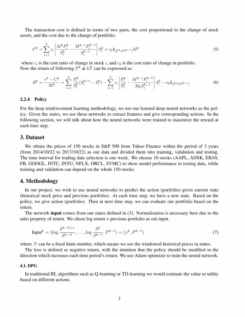
The transaction cost is defined in terms of two parts, the cost proportional to the change of stockassets, and the cost due to the change of portfolio:
Ck =L∑i=1
ci
∣∣∣∣∣MkP kiSki
−Mk−1P k−1i
Sk−1i
∣∣∣∣∣Ski + c01[Pk 6=Pk−1]Mk (5)
where ci is the cost ratio of change in stock i, and c0 is the cost ratio of change in portfolio.Now the return of following P k at kT can be expressed as:
Rk =rk − Ck
Mk=
L∑i=1
P kiSki
(Sk+1i − Ski )−
L∑i=1
ci
∣∣∣∣∣P kiSki − Mk−1P k−1i
MkSk−1i
∣∣∣∣∣Ski − c01[Pk 6=Pk−1] (6)
2.2.4 Policy
For the deep reinforcement learning methodology, we use our learned deep neural networks as the pol-icy. Given the states, we use these networks to extract features and give corresponding actions. In thefollowing section, we will talk about how the neural networks were trained to maximize the reward ateach time step.
3. DatasetWe obtain the prices of 150 stocks in S&P 500 from Yahoo Finance within the period of 3 years
(from 2014/10/22 to 2017/10/22) as our data and divided them into training, validation and testing.The time interval for trading date selection is one week. We choose 10 stocks (AAPL, ADSK, EBAY,FB, GOOGL, INTC, INTU, NFLX, ORCL, SYMC) to show model performance in testing data, whiletraining and validation can depend on the whole 150 stocks.
4. MethodologyIn our project, we wish to use neural networks to predict the action (portfolio) given current state
(historical stock price and previous portfolio). At each time step, we have a new state. Based on thepolicy, we give action (portfolio). Then at next time step, we can evaluate our portfolio based on thereturn.
The network input comes from our states defined in (3). Normalization is necessary here due to theratio property of return. We chose log return + previous portfolio as out input.
Inputk = (logSk−N+1
Sk−N, . . . , log
Sk
Sk−1, P k−1) = (xk, P k−1) (7)
where N can be a fixed finite number, which means we use the windowed historical prices in states.The loss is defined as negative return, with the intuition that the policy should be modified in the
direction which increases each time period’s return. We use Adam optimizer to train the neural network.
4.1. DPG
In traditional RL algorithms such as Q-learning or TD-learning we would estimate the value or utilitybased on different actions.
3

Suppose we have policy π. The reward we are going to collect at the next state s′ is r(s, π(s), s′). Theexpected reward from a stochastic policy is
r(s, π(s), s′) =∑a
pπ(s, a, s′)r(s, a, s′) (8)
However when action is in continuous space the curse of dimensionality dominates - the total number ofactions increases exponentially as the discretization precision increases. It was proposed by [9][10] tothrow away the stochasticity and produce an deterministic action for continuous space action and thenevaluate and update parameters accordingly. Hence at each time step we can just produce one actionbased on policy π and make further updates based on it.
In our case, we use neural networks to produce the action of the next time step based on currentstate. The gradients will be calculated by first backpropagating through 6 to the action and then back-propagating in the neural nets (which is automatically taken care of by deep learning libraries such asTensorFlow).
4.2. CNN
For finite historical time dependency, which assumes current optimal portfolio only depends on finiteN historical stock prices, CNN can be a good choice. In this way, the state inputs we defined share manyitems sequentially. Specifically, this is a stride of LogReturn in time domain, which is very similar tothe image patch in image processing, thus motivates us to use CNN for this scenario.
Each input is a N × L log return matrix plus a vector of previous portfolio with length L. Firstly,for each stock we output a score based only on this stock’s historical return and its previous portfoliopercentage using CNN and then the scores are combined using a softmax to produce a distribution whichbecomes our action (portfolio). The architecture of the neural network is shown in Figure 1.
Figure 1. Architecture diagram of CNN model.
4.3. RNN
Compared to feed-forward neural nets, RNN has the advantage of being able to take input sequenceof arbitrary length. For basic RNN cell, the relation can be expressed as
ht = f(Wh ∗ ht−1 +Wx ∗ xt) (9)
4
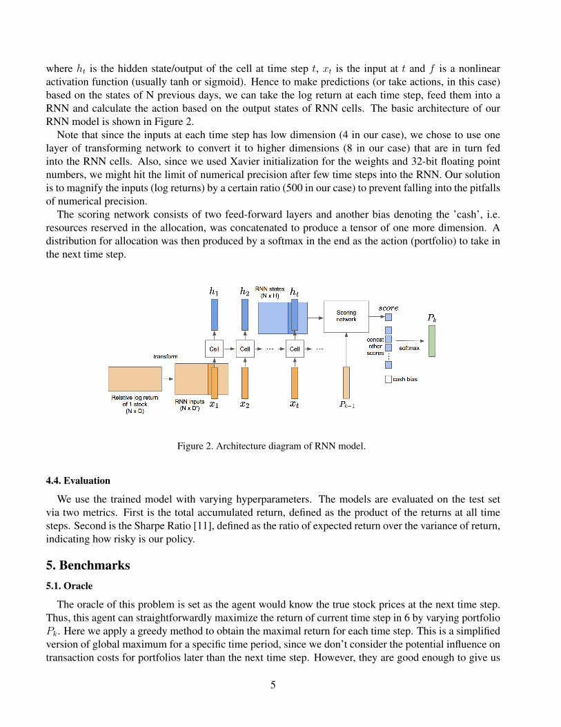
where ht is the hidden state/output of the cell at time step t, xt is the input at t and f is a nonlinearactivation function (usually tanh or sigmoid). Hence to make predictions (or take actions, in this case)based on the states of N previous days, we can take the log return at each time step, feed them into aRNN and calculate the action based on the output states of RNN cells. The basic architecture of ourRNN model is shown in Figure 2.
Note that since the inputs at each time step has low dimension (4 in our case), we chose to use onelayer of transforming network to convert it to higher dimensions (8 in our case) that are in turn fedinto the RNN cells. Also, since we used Xavier initialization for the weights and 32-bit floating pointnumbers, we might hit the limit of numerical precision after few time steps into the RNN. Our solutionis to magnify the inputs (log returns) by a certain ratio (500 in our case) to prevent falling into the pitfallsof numerical precision.
The scoring network consists of two feed-forward layers and another bias denoting the ’cash’, i.e.resources reserved in the allocation, was concatenated to produce a tensor of one more dimension. Adistribution for allocation was then produced by a softmax in the end as the action (portfolio) to take inthe next time step.
Figure 2. Architecture diagram of RNN model.
4.4. Evaluation
We use the trained model with varying hyperparameters. The models are evaluated on the test setvia two metrics. First is the total accumulated return, defined as the product of the returns at all timesteps. Second is the Sharpe Ratio [11], defined as the ratio of expected return over the variance of return,indicating how risky is our policy.
5. Benchmarks5.1. Oracle
The oracle of this problem is set as the agent would know the true stock prices at the next time step.Thus, this agent can straightforwardly maximize the return of current time step in 6 by varying portfolioPk. Here we apply a greedy method to obtain the maximal return for each time step. This is a simplifiedversion of global maximum for a specific time period, since we don’t consider the potential influence ontransaction costs for portfolios later than the next time step. However, they are good enough to give us
5

an idea of how well the agent can possibly perform. Specifically, we use cvxpy package to obtain theoracle.
5.2. Baseline
The baseline of this problem is chosen to be the well-known Eigen-portfolio used in tons of financialliterature. For time period [kT, (k + 1)T ], denote expected return for different stocks are E[rk] =(E[rk1 ], . . . , E[r
kL]). The eigen-portfolio idea is as follows: given a portfolio P k, we hope to maximize
E[P k · rk]. Denote cov(rk) is the covariance of Return for L stocks, then the normalized eigenvectorwith largest eigenvalue of cov(rk) is called eigen-portfolio, which has been empirically verified to havethe largest correlation with the market.
In order to estimate covariance matrix cov(rk), we use the weighted average based on the historicaldata. Here we choose the exponential weights, that is, for data from [(k− p)T, (k− p+1)T ], the weightis exp(−(pµ))/C, where µ is a model parameter and C is the denominator for normalization.
E(rk) =
P∑p=1
exp(−(pµ))C
rk−p
ˆcov(rk) =P∑p=1
exp(−(pµ))C
× (rk−p − E((rk−p))(rk−p − E((rk−p))T
(10)
µ is selected by using the precedent time step as validation data. After getting eigen-porfolio, we use(6) to calculate return with transaction costs.
5.3. Best Stock
Best Stock is a benchmark method where the agent knows each stock’s growth rate between day oneand the last day of consideration, which is (Sfinali − S1
i )/S1i . The agent just invests all its assets on one
stock with the highest such growth rate, and hold it during the whole time period. In this case, each timestep’s return equals to the growth rate of one best stock.
5.4. Uniform Buy And Hold
We use another benchmark, Uniform Buy And Hold (UBAH), to show how well the agent can performwithout any non-trivial strategies. In UBAH, the agent distributes its assets uniformly among all studiedstocks. We hope this method can provide us a bottom line for the agent’s performance.
6. ExperimentsWe conducted extensive analysis of the models based on various hyperparameters such as the number
of days to look back, the size of CNN kernels and RNN cell hidden size. As stated above, we evaluatethe performances based on the total return (TR) and Sharpe Ratio (SR).
The training, validation and testing data date are [11/05/2014, 02/08/2017], [02/15/2017, 05/24/2017],[05/31/2017, 10/18/2017] separately. We did model sensitivity analysis on validation data and com-pared different model performances on testing data.
6

6.1. Sensitivity Analysis
6.1.1 CNN
The weekly return and accumulated return of CNN model under different kernelsize k with N = 10 anddifferent N with k = 3 is shown in Figures 3 and 4. We can find that varying kernel size k and N doesnot influence much on total return, while sharpe ratio could be different with different k and N . The besthyperparameters we choose here is N = 10, k = 3, which achieves best sharpe ratio on validation data.
Figure 3. The effect of k (convolutional kernel size) on CNN performance.
Figure 4. The effect of N (number of days looking back) on CNN performance.
6.1.2 RNN
The weekly return and accumulated return of our RNN model under different kernel sizes are shownin Figures 5 and 6. Based on the total return and sharper ratio, we find that HS and N’s influences arenot smooth. In this way, we choose our best hyperparameters only by selecting ones with highest totalreturn and sharpe ratio (HS = 7, N = 7).
7

Figure 5. The effect of HS (hidden size of RNN cell) on RNN performance.
Figure 6. The effect of N (number of days looking back) on RNN performance.
6.2. Model Comparison and Analysis
Figure 7 shows the performances of all our models along with the established benchmarks. Thesemodels can be divided into two categories: category one using future data—Oracle and Best Stock—and category two only using historical data: Baseline, CNN, RNN and Uniform Buy and Hold.
For category One, portfolio management is trivial because we have known the tendency of the stockprices. There is no surprise that Oracle is powerful and outperforms all other models.
For category Two, we can see that CNN outperforms all others in the end, showing the effectivenessof our reinforcement learning policy and the potential that useful information can be extracted fromhistorical stock prices to predict the future. Note that CNN has poorer performance than baseline at thebeginning, and later becomes better, which is coherent with online learning update while our policy getsbetter during the reinforcement learning as time continues.
However, the stock data is noisy and many outside factors other than historical prices can influencethe price trend, which limits the ability of our model. Another noticeable thing is that RNN does notoutperform CNN and Uniform Buy and Hold, which is against our previous expectation, because RNNcan be asymptotically considered as depending on infinite history while CNN only depends on finitehistory and Uniform Buy and Hold does not pay attention to price tendency. This could be due to thatthe RNN cell we used is not complex enough and the price data is highly noisy which impacts RNNlearning.
8

Figure 7. Comparison of all models and benchmarks.
7. ConclusionIn this project, we have formulated the portfolio management problem into a deep RL problem with
DPG. We successfully implemented the models in TensorFlow and trained on historical data from S&P500.
At the end the test results of our models only surpassed the baseline by a slight margin. It is possiblethat the results are caused by the following reasons: 1. Deep learning models tend to have high variance,which makes them hard to train on financial data with high noise. 2. Our data might be insufficient.Some work [6] train their models on crytocurrency data taken every 30 min. Our model was trained onstock prices every week. 3. The network structures require more refinement, e.g. the softmax operationat the end might be problematic because it changes a possibly linear scale in the scores to a exponentialscale, or the cash bias should be a parameter to be learned instead of setting to 0 for cash. 4. More usefuloutside information other than historical stock prices can be integrated into networks such as news andfiscal policies.
To improve this project, one way is to train on a larger dataset (preferably with cryptocurrency data)and also take into account the interactions between assets. Another way is to integrate other inputssuch as news sentiment into the network to help make better decisions. Also, the network structure issomething we can work on. We could change how we calculated action based on scores as discussedabove. We could also try to use other innovative architectures such as actor-critic [10] to help learning.To reduce the variance of the models, mechanisms such as attention [12] and dropout [13][14] can beapplied as well. Deep learning in finance is very promising since it might be able to capture someinformation is an extremely complicated environment.
References[1] Modern Invest Theory, Robert A. Haugen, Prentice Hall, 1986
[2] Online portfolio selection: A survey, Bin Li and Steven CH Hoi, ACM Computing Serveys (CSUR), 46(3):35,2014
9

[3] Nonparametric Kernel-based Sequential Investment Strategies, Laszlo Gyorfi, Gabor Lugosi, and FredericUdina, Mathematical Finance, 16(2):337357, 2006
[4] Deep learning for finance: deep portfolios, J. B. Heaton, N. G. Polson, and Jan Hendrik Witte, AppliedStochastic Models in Business and Industry, 2016, ISSN 1526-4025. doi: 10.1002/ASMB.2209
[5] Forecasting S&P 500 index using artificial neural networks and design of experiments, Seyed Taghi AkhavanNiaki and Saeid Hoseinzade, Journal of Industrial Engineering International, 9(1):1, 2013. ISSN 2251-712X.doi: 10.1186/2251-712X-9-1
[6] Deep direct rein- forcement learning for financial signal representation and trading, Yue Deng, Feng Bao,Youyong Kong, Zhiquan Ren, and Qionghai Dai, IEEE transactions on neural networks and learning systems,28(3):653664, 2017
[7] A Deep Reinforcement Learning Framework for the Financial Portfolio Management Problem, ZhengyaoJiang, Dixing Xu, Jinjun Liang, arXiv:1706.10059v2
[8] https://github.com/wassname/rl-portfolio-management
[9] Deterministic Policy Gradient Algorithms, Silver et al, arXiv:1509.02971
[10] Deep Deterministic Policy Gradients, Lillicrap et al, arXiv:1509.02971
[11] The sharpe ratio, Sharpe, W. F. (1994), The Journal of Portfolio Management, 21(1), 49-58.
[12] Effective Approaches to Attention-based Neural Machine Translation, Luong et al, arXiv:1508.04025
[13] Improving deep neural networks for lvcsr using rectified linear units and dropout, Dahl et al, IEEE 2013,DOI: 10.1109/ICASSP.2013.6639346
[14] Understanding the dropout strategy and analyzing its effectiveness on LVCSR, Li et al, IEEE 2013, DOI:10.1109/ICASSP.2013.6639144
10


