Download - Deformation of Minimal Polynomials and Approximation of Several Intervals by an Inverse Polynomial Mapping

Journal of Approximation Theory 111, 180�195 (2001)

Deformation of Minimal Polynomials and Approximationof Several Intervals by an Inverse Polynomial Mapping

Franz Peherstorfer1

Johannes Kepler Universita� t Linz, Institut fu� r Analysis und Numerik,Linz-Auhof A-4040, Austria

Communicated by Vilmos Totik

Received March 15, 1999; accepted in revised form February 20, 2001;published online June 20, 2001

In this paper we show that for a given set of l real disjoint intervalsEl=� l

j=1 [a2 j&1 , a2 j] and given =>0 there exists a real polynomial T and a setof l disjoint intervals E� l=� l

j=1 [a~ 2 j&1 , a~ 2j] with E� l $El and &(a~ 1 , ..., a~ 2l)&(a1 , ..., a2l)&max<=, such that T&1([&1, 1])=E� l . The statement follows by showinghow to get in a constructive way by a continuous deformation procedure from aminimal polynomial on El with respect to the maximum norm a polynomial map-ping of E� l . � 2001 Academic Press

1. SOME BASIC FACTS ON T- AND MINIMAL POLYNOMIALSAND INVERSE POLYNOMIAL MAPPINGS

Let l # N, a1 , a2 , ..., a2l # R, a1<a2< } } } <a2l , and let

El := .l

j=1

[a2 j&1 , a2 j] and H(x) := `2l

j=1

(x&aj). (1.1)

Note that H(x)�0 for x # El . As usual, let Pn , n # N0 , denote the set ofreal polynomials of degree less or equal n. If pn(x)=dnxn+ } } } # Pn "Pn&1

then p̂n(x)= pn(x)�dn denotes the monic polynomial of degree n. A pointy # El is called extremal point (abbreviated e-point) of p # Pn on El if| p( y)|=&p&El

, where &p&El:=maxx # El

| p(x)|. e-points from Int(El)and from �El are called interior and boundary e-points, respectively. Thepoints x1 , x2 , ..., xm # El , x1<x2< } } } <xm , are called alternation points

doi:10.1006�jath.2001.3571, available online at http:��www.idealibrary.com on

1800021-9045�01 �35.00Copyright � 2001 by Academic PressAll rights of reproduction in any form reserved.

1 This work was supported by the Austrian Science Fund FWF, project-number P12985-TEC.

(abbreviated a-points) of p on El if they are e-points of p and p(xj)=& p(xj+1) for j=1, 2, ..., m&1. Finally, a monic polynomial Mn(x)=xn+ } } } is called minimal polynomial on El if

mincj # R

&xn+cn&1 xn&1+ } } } +c1x+c0&El=&Mn(x)&El

.

Let us recall that by the Alternation-Theorem Mn is a minimal polynomialon El if and only if it has n+1 alternation points on El .

In this paper Chebyshev-polynomials (abbreviated T-polynomials) onEl , which we define in the following way, will play an important role.

Definition 1.1. A polynomial Tn(x)=cn xn+ } } } # Pn , n # N, cn # R"

[0], is called T-polynomial on El if it has n+l e-points on El . A T-polyno-mial of degree n on El is denoted by Tn(x, El) where El is omitted if thereis no danger of confusion. The polynomial T� n(x, El)=Tn(x, El)�&Tn(x, El)&El

is called normed T-polynomial on El .

Naturally, the classical T-polynomial of the first kind Tn(x)=cos n arccos x, x # [&1, 1], is a normed T-polynomial on [&1, 1] for which theinterior e-points are given by the zeros of Un&1(x)=sin n arc cos x�sin arc cos x. T-polynomials on two intervals have been studied by Achieser[1, 3], see also [18], with the help of elliptic functions and by the authorin [14, 15] with the help of orthogonal polynomials. The case of severalintervals has been investigated by the author in [16, Section 2], [17], seealso [25]. The reason why we called these polynomials T-polynomials isthat they share many properties with the classical T-polynomials, as thenext proposition shows.

Proposition 1.1 ([16, Section 2], [17]).

(i) Let Tn be a T-polynomial on El , then Tn has the following properties:

(i1) Tn has exactly n&l interior e-points z1 , z2 , ..., zn&l # Int(El)and the 2l boundary e-points a1 , a2 , ..., a2l # �El . Moreover, Tn has n+1a-points on El , thus the monic T-polynomial T� n(x)=xn+ } } } is also theminimal polynomial on El .

(i2) T$n has, besides the n&l simple zeros z1 , z2 , ..., zn&l # Int(El),exactly one zero dj in each gap (a2 j , a2 j+1), j=1, 2, ..., l&1. Furthermore,Tn has n simple zeros in Int(El) and El=T� &1

n ([&1, 1]).

(i3) If Tn is a T-polynomial on El , then Tk(T� n), k # N, areT-polynomials of degree kn on El . Furthermore, if there exists no otherT-polynomial on El of degree less than n, then the polynomials Tk(T� n), k # N,are the only T-polynomials on El .

181INVERSE POLYNOMIAL MAPPING

(ii) Tn is a T-polynomial on El if and only if there exists a polynomialUn&l # Pn&l with n&l simple zeros in Int(El), such that

T2n(x)=H(x)U2

n&l (x)+L2, (1.2)

where H is defined in (1.1) and L # R"[0].

(iii) If Tn(x)=xn+ } } } # Pn is a T-polynomial on El , then

T$n(x)=nUn&l (x) rl&1(x), where rl&1(x) := `l&1

j=1

(x&dj), (1.3)

where Un&l is given by (1.2) and the dj 's are defined in (i2). Furthermore, by(1.2), U� n&l is the minimal polynomial of degree n&l on El with respect tothe weight function - &H(x).

(iv) Let pn(x)=cn xn+ } } } # Pn , cn {0, be a polynomial with n simplereal zeros and K :=min[ | pn(x)|: p$n(x)=0], then, for every + # (0, K],Tn, +(x) := 1

+ pn(x) is a T-polynomial on the set of intervals T� &1n, +([&1, 1]).

(v) There exists a T-polynomial Tn on E l with mj+1 e-points on[a2 j&1 , a2 j], j=1, 2, ..., l, if and only if there are l integers mj # [1, ..., n&l]with � l

j=1 mj=n, such that

1

? |a2 j

a2 j&1

|rl&1(x)|

- |H(x)|dx=

mj

n, j=1, 2, ..., l, (1.4)

where rl&1(x)=xl&1+ } } } is the unique polynomial that satisfies

|a2 j+1

a2 j

rl&1(x)

- |H(x)|dx=0, j=1, 2, ..., l&1. (1.5)

Furthermore, if there exists a T-polynomial Tn on El , then T� n is given by

T� n(z)=cosh \n |z

a1

rl&1(x)

- H(x)dx+ , (1.6)

where the polynomial rl&1 which satisfies (1.5) is identical to the polynomialrl&1 from (1.3).

In [16], T-polynomials have been defined by relation (1.2). Let us alsomention that in the single interval case E1=[&1, 1], relation (1.2) becomesthe well known relation for classical T-polynomials of the first and secondkind

T 2n(x)+(x2&1)U 2

n&1(x)=1.

182 FRANZ PEHERSTORFER

As already mentioned a monic T-polynomial Tn on El is a minimal poly-nomial on El which has the additional property that |Tn |>1 on R"E l . Theprecise connection between T- and minimal polynomials is given in part (ii)of the following proposition.

Proposition 1.2. (i) Let (nk) be a subsequence of the natural numbersand let for k # N Mnk

be the minimal polynomial on the compact set K(nk)�[a, b], a<b. Then within K(nk) the distance of two consecutive alternationpoints is at most O(1�nk).

(ii) If Mn is a minimal polynomial on E l then Mn is a T-polynomial onl*=l+l $, 0�l $�l&1, intervals E*l*, n

E*l*, n= .l

j=1

[a2 j&1, n , a2 j, n] _ .l $

&=1

[c2 j&&1, n , c2 j& , n],

j& # [1, ..., l&1] for &=1, ..., l $, where a1, n=a1 , a2l, n=a2l ,

a2 j�a2 j, n<a2 j+1, n�a2 j+1 and a2 j, n=a2n or a2 j+1, n=a2 j+1

for j=1, ..., l&1 and

a2 j& , n=a2 j&<c2 j&&1, n<c2 j& , n<a2 j&+1, n=a2 j&+1 for &=1, ..., l $.

Furthermore, on each ``c-interval '' [c2 j&&1, n , c2 j& , n], &=1, ..., l $, Mn has nointerior e-point and Mn is a minimal polynomial on every subset of E*l*, n

which contains El . Finally, if we write E*l*, n=El, n _ Cl $, n then

El, n ww�n � �

El and limn � �

*(Cl $, n)=0,

where * denotes the Lebesgue-measure.

Proof. Part (i) follows by slightly modifying the proof of Theorem 1 in[10]. Indeed, in the first part of the proof replace [a, b] by K(nk) and let: and ; be two consecutive alternation points of Mnk

within K(nk). Notethat in the case under consideration r=kn=sn=0. Then it follows that theminimum deviation of f, f defined in [10], with respect to Pnk

on K(nk) is�1. Hence, f extended to [a, b] by f#0 on [a, b]"K(nk) has also mini-mum deviation �1 on [a, b] with respect to Pnk

. Now proceeding wordby word as in the last lines of the proof of Theorem 1 the assertion follows.

Up to the limit relations part (ii) follows immediately with the help ofthe Alternation-Theorem and by a careful counting of the zeros of thederivative of Mn as already mentioned in [16]. Both limit relations followimmediately from part (i). K


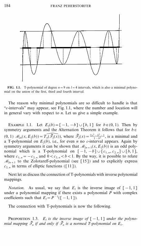
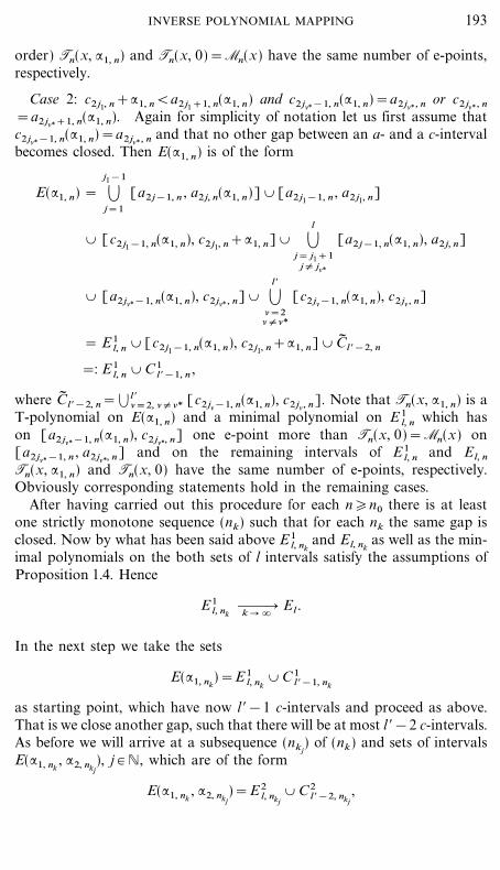
FIG. 1.1. T-polynomial of degree n=9 on l=4 intervals, which is also a minimal polyno-mial on the union of the first, third and fourth interval.

The reason why minimal polynomials are so difficult to handle is that``c-intervals'' may appear, see Fig. 1.1, where the number and location willin general vary with respect to n. Let us give a simple example.

Example 1.1. Let E2(b)=[&1, &b] _ [b, 1] for b # (0, 1). Then bysymmetry arguments and the Alternation Theorem it follows that for b #

(0, 1) M2n(x, E2(b))=Tn(T� 2(x))@ , where T� 2(x)= 2x2&b2&11&b2 , is a minimal and

a T-polynomial on E2(b), i.e., for even n no c-interval appears. Again bysymmetry arguments it can be shown that M2n+1(x, E2(b)) is an odd poly-nomial which is a T-polynomial on [&1, &b] _ [c1, n , c2, n] _ [b, 1],where c1, n=&c2, n and 0<c2, n<b<1. By the way, it is possible to relateM2n+1 to the Zolotareff-polynomial (see [15]) and to explicitly expressc2, n in terms of elliptic functions ([11]).

Next let us discuss the connection of T-polynomials with inverse polynomialmappings.

Notation. As usual, we say that El is the inverse image of [&1, 1]under a polynomial mapping if there exists a polynomial P with complexcoefficients such that El=P&1([&1, 1]).

The connection with T-polynomials is now the following.

Proposition 1.3. El is the inverse image of [&1, 1] under the polyno-mial mapping T� n if and only if T� n is a normed T-polynomial on El .


Proof. The sufficiency part of the proof follows immediately from point(i2) of Proposition 1.1. For the necessity part see [20, Proposition 2]. K

Inverse polynomial images of arbitrary compact sets K of the complexplane, in particular of the interval [&1, 1], have been studied in [6�8, 19,20, 22]. One of the main reasons why these sets are of foremost interest isthat frequently properties on K are inherited in a suitable way to theinverse image T&1

n (K). So certain extremal problems are easy to handle onan inverse polynomial image of [&1, 1] (for instance if pj is an Lq(+)-mini-mal polynomial on [&1, 1], q # [1, �], then pj b Tn is an Lq(+Tn)-minimalpolynomial on T&1

n ([&1, 1]), see [22] for details), but not on anarbitrary set of intervals. Therefore the question arises whether a given setof intervals can be approximated arbitrarily well by polynomial inverseimages. In order to be able to treat this question we need some facts frompotential theory (see e.g. [9, 27]).

Let G(z, �)= g(z, �)+ig~ (z, �) be the complex Green function ofG=C _ [�]"El with pole at �, i.e., g( } , �) is harmonic in G"[�] witha behaviour at � given by

g(z, �)=ln |z|+harmonic function

and

limG % z � x

g(z, �)=0 for x # El ,

where g~ (z, �) is a harmonic conjugate of g. It is well known that g(z, �)can be represented in the form

g(z, �)=|El

ln |z&x| d&El (x)&ln cap(El),

where &El is the so-called equilibrium (Frostman) measure of El andcap(El) is the capacity of El . Recall (see e.g. [24, Section III]) that

limn � �

&Mn(x, El)&1�nEl

=cap(El), (1.7)

where Mn(x, El) is the monic minimal polynomial on El , and that (1.7)implies that the zero counting measure of Mn(x, El)=>n

j=1 (x&xj, n)converges in the weak star sense to the equilibrium measure of El , i.e.,

1n

:n

j=1

$xj , n ww�V

n � �&El , (1.8)


where $xj , n denotes, as usual, the Dirac-Delta measure at the point xj, n .Furthermore it is known (see [28, Section 14]) that the complex Greenfunction of El is of the form

G(z, �)=|z

a1

rl&1(!)

- >2lj=1 (!&aj)

d!, (1.9)

where the integration is performed along a path in the complex plane cutalong El and where rl&1(!)=! l&1+ } } } # Pl&1 is that unique polynomialwhich satisfies

|a2 j+1

a2 j

rl&1(x)

- >2lj=1 (x&aj)

dx=0 for j=1, ..., l&1. (1.10)

Hence

|El

d&(x)z&x

=G$(z, �)=rl&1(z)

- H(z),

which gives with the help of the Sochozki�Plemelj formula that theequilibrium measure & for El is given by (see [13, Lemma 1])

&$(x)={ |rl&1(x)|�? - &H(x)0

for x # E l

elsewhere.(1.11)

Let us note that condition (1.10) implies that rl&1 has exactly one zero ineach gap (a2 j , a2 j+1), j=1, ..., l&1. We also would like to point out thatthe polynomial rl&1 satisfying condition (1.10) is known if there is aT-polynomial Tn on El . Indeed, by Proposition 1.1(v) it is the polynomialrl&1 from (1.3).

Now let us recall that the following relation holds between theequilibrium measure and the harmonic measure for C� "El (see e.g.[23, Thm. 4.3.14]):

&(B)=|(�, B, C� "El) for any Borel subset B of El . (1.12)

As usual, |(z, B, C� "El), z # C� "El , denotes the harmonic measure for C� "El

of B�El which is that harmonic and bounded function on C� "El whichsatisfies for ` # El that limz � ` |(z, B, C� "El)=iB(`), where iB denotes, asusual, the characteristic function of B.


Thus (v) in Proposition 1.1 can be expressed in the following way. Thereexists a T-polynomial Tn on El with m j+1 e-points on [a2 j&1 , a2 j], j=1, ..., l, if and only if there are l natural numbers mj # [1, 2, ..., n&l] with�l

j=1 mj=n such that the harmonic measure satisfies

|(�, [a2 j&1 , a2 j], C� "El)=mj

nfor j=1, ..., l.

This form of the Proposition has been proved in [4] with the help of deepresults of Widom [28] on the asymptotics of orthogonal polynomials.

Lemma 1.1. Let El�E� l and let us assume that [a2 j*&1 , a2 j*] is a com-ponent of both El and E� l and that E� l"El $[c, d], c<d. Then &El ([a2 j*&1 ,a2 j*])&&E� l ([a2 j*&1 , a2 j*])>0.

Proof. Let us consider the two harmonic measures |(z, [a2 j*&1 , a2 j*],C� "El) and |(z, [a2 j*&1 , a2 j*], C� "E� l). Since E� l"El $[c, d], we have by theCarleman extension principle (see e.g. [12, IV, Section 2])

|(z, [a2 j*&1 , a2 j*], C� "El)&|(z, [a2 j*&1 , a2 j*], C� "E� l)>0 (1.13)

on each compact subset of C� "E� l . Considering (1.13) at the point z=� andrecalling relation (1.12) the lemma is proved. K

In the following let *E(Mn , B), B�El , denote the number of e-pointsof Mn( } , El) on B. With the help of Lemma 1.1 we obtain

Proposition 1.4. Let (nk) be a strictly monotone subsequence of thenatural numbers. Suppose that for each k # N El �El, nk=� l

j=1 [a2 j&1, nk ,a2 j, nk]�E� l, nk=� l

j=1[a~ 2 j&1, nk , a~ 2 j, nk] with a1=a1, nk=a~ 1, nk<a2�a2, nk�a~ 2, nk<a~ 3, nk�a3, nk�a3<a4�a4, nk�a~ 4, nk< } } } <a~ 2l&1, nk�a2l&1, nk�a2l&1

<a2l=a2l, nk=a~ 2l, nk , that E� l, nk and El, nk have a common component[a2 j*&1, nk , a2 j*, nk]=[a~ 2 j*&1, nk , a~ 2 j*, nk] and that El, nk ww�

k � �El . Further-

more let us assume that for all k # N0 the minimal polynomials Mnk and M� nk

on El, nk and E� l, nk , respectively, have the property that

*E(M� nk , [a~ 2 j&1, nk , a~ 2 j, nk])&*E(Mnk , [a2 j&1, nk , a2 j, nk])

�const for j=1, ..., l.

Then the following statement holds:

E� l, nk ww�k � �

El . (1.14)


Proof. Let us suppose that there is a subsequence of (nk) denoted by(nk) again such that E� l, nk ww3 �

k � �El , that is, if necessary by taking another

subsequence of (nk), that

E� l, nk � E� l= .l

j=1

[a~ 2 j&1 , a~ 2 j] where E� l"El $[c, d], c<d.

Then E� l and El have the common component [a2 j*&1 , a2 j*] and thus byLemma 1.1

0<&El ([a2 j*&1 , a2 j*])&&E� l ([a2 j*&1 , a2 j*]). (1.15)

On the other hand it is known (see [24, Section III]) that

limk � �

&Mk &1�nkEl, nk

=cap(El) and limk � �

&M� nk &1�nkE� l, nk

=cap(E� l) (1.16)

and that (1.16) implies that the zero counting measure of Mnk and M� nk

converges in the weak star sense to the equilibrium measure of El and E� l ,respectively. More precisely, if Mnk(x)=>nk

j=1 (x&x j, nk) and M� nk(x)=>nk

j=1 (x&x~ j, nk), then

1nk

:nk

j=1

$xj , nkww�

Vk � �

&El and1

nk:nk

j=1

$x~ j , nkww�

Vk � �

&E� l , (1.17)

where $xj is the Dirac-Delta measure at the point xj . Since the zerodistribution is the same as that of the e-points it follows from (1.17) andthe assumption on the e-points that

&El ([a2 j&1 , a2 j])=&E� l ([a~ 2 j&1 , a~ 2 j]) for j=1, ..., l.

But this is a contradiction to (1.15). K

By the suggestions of the referee the proof of Proposition 1.4 becameessentially nicer and shorter.

Let us point out that it is essential that E� l, nk and El, nk have a commoncomponent as the Example 1.1 shows. Put El, 2n=El=E2(b) and E� l, 2n=E2(b$) with 0<b<b$ there and observe that the even minimal polynomialsM2n and M� 2n have exactly n+1 e-points in [b, 1] and [b$, 1], respectively.

2. MAIN RESULT

Now we are ready to treat the question whether the set of l intervals onwhich there exists a T-polynomial is dense in the set of l intervals.


For l=2 the denseness has been proved by Achieser [2] with the helpof elliptic functions and later by Atlestam [5] by showing that for given a3

h(a2)=|a2

&1

|r1(x)|

- (1&x2)(x&a2)(x&a3)dx

is a bijective mapping on (&1, a3). Both methods turned out to be unsuitablefor the proof of the general case of l intervals.

We shall give a constructive proof by showing how to get by a continuousdeformation procedure from a minimal polynomial on El a T-polynomialon E� l , i.e., the desired polynomial mapping. The procedure is based on thefollowing proposition.

Proposition 2.1. Let Tn be a T-polynomial on � lj=1 [a2 j&1 , a2 j] and

let j* # [2, 3, ..., l&1]. Then there exists an :*>0 such that there arestrictly monotone increasing functions a2 j (:): [0, :*] � [a2 j , a2 j+1] forj=1, 2, ..., j*&1, and a2 j*&1(:): [0, :*] � [a2 j*&1 , a2 j*+1), as well asstrictly monotone decreasing functions a2 j&1(:): [0, :*] � [a2 j&2 , a2 j&1]for j= j*+1, ..., l such that the following statements hold:

(i) For each : # [0, :*] there exists a T-polynomial Tn(x, :) on

El (:)= .j*&2

j=1

[a2 j&1 , a2 j (:)] _ [a2 j*&3 , a2 j*&2]

_ [a2 j*&1(:), a2 j*+:] _ .l

j= j*+1

[a2 j&1(:), a2 j].

Furthermore, for : # [0, :*) El (:) consists of l disjoint intervals and Tn(x, :)has on the first, second, third, ... interval of El (:) the same number of e-pointsas Tn(x) on the first, second, third, ... interval of El and all interior e-pointswhich are smaller resp. larger than a2 j* increase resp. decrease with respectto :.

(ii) For :=:* there exists a + # [1, 2, ..., j*&2] or a + # [ j*+1, ..., l] such that a2+(:*)=a2++1 , + # [1, 2, ..., j*&2], or a2+&1(:*)=a2+&2 , + # [ j*+2, ..., l], or a2 j*+1(:*)=a2 j*+:*, i.e., for :=:* at leastone gap is closed. Furthermore, no interior e-points coalesce.

Proof. The proof runs in a similar way as the proof of Theorem 2.9 in[21]. Let us prove the assertion for small :>0 first. Let d0=(d 0

1 , ..., d 0n&1),

where [d 0j ]n&1

j=1 consists of all interior e-points of Tn and the l&1 boundarypoints a2 , a4 , ..., a2( j*&2) , a2 j*&1 , a2 j*+1 , ..., a2l&1 . Furthermore let

c=(a1 , a3 , ..., a2 j*&5 , a2 j*&3 , a2 j*&2 , a2 j*+:, a2 j*+2 , a2 j*+4 , ..., a2l) # Rl+1


and for :=0 let us denote this vector by c0. Then it follows by Theorem 2.7of [21] that for sufficiently small :>0 there is a vector

d(c)=(d1(c), ..., dn&1(c))

with d(c0)=d0 such that E(b)=�nj=1 [b2 j&1 , b2 j], where [bj]2n

j=1=[c&] l+1&=1

_ [d}(c)]n&1}=1 , b1<b2� } } } �b2n&1<b2n , consists of l disjoint intervals

and on E(b)=: El (:) there exists a T-polynomial Tn(x, b)=: Tn(x, :) whichhas the same number of e-points on each of the l disjoint intervals of El (:)as Tn on the corresponding intervals of El .

Concerning the monotonicity let us first note that besides the n&l interiore-points of Tn(x, :) all l&1 nonfixed boundary points a2(:), a4(:), ...,a2( j*&2)(:), a2 j*&1(:), a2 j*+1(:), ..., a2l&1(:) are contained in [dj (c)]n&1

j=1 .Now we claim that for each d}(c) from [dj (c)]n&1

j=1 we have

sgn Tn(d}(c), :)=&sgn `n&1

j=1j{}

(d}(c)&d j (c)). (2.1)

Indeed, if d}(c)�a2 j*&1(:) then (2.1) follows from the observation that

sgn Tn(d}(c), :)=(&1)1+n}+

,

where n+} denotes the number of dj (c)$s which lie at the right hand side of

d}(c). If d}(c)<a2 j*&2 then

sgn Tn(d}(c), :)=(&1)n&(1+n}&),

where n&} denotes the number of dj (c)$s which lie at the left side of d}(c).

This proves (2.1).Next let

cj*+1=a2 j*+:

be the ( j*+1)th component of c. Then we have by the relations (2.19) and(2.20) of [21] and (2.1) that

�d}

�cj*+1

(c)=&sgn \Tn(a2 j*+:, :)Tn(d}(:), :)

} `n&1

j=1j{}

a2 j*+:&dj (c)d}(c)&dj (c) +

=sgn(a2 j+:&d}(c)), (2.2)

where in the last equality we have used the fact that

sgn Tn(a2 j*+:, :)= `n&1

j=1

(a2 j*+:&d j (c)),


which proves the monotonicity property. Thus the theorem is proved forsmall :>0.

The remaining part of the proof runs now in almost the same way as theproof of Theorem 2.9 in [21], more precisely as the part beginning threelines before relation (2.27). Indeed, since by [21, Corollary 2.5] theexistence of the T-polynomial Tn(x, :) is equivalent to

|Et (:)

xk sgn[ p (:)n&1(x)] dx=0, k=0, ..., n&2, (2.3)

where

p (:)n&1(x)= `

n&1

j=1

(x&dj (c)),

it follows as in [21] that no interior e-point can coincide with anothere-point as : � $ because then we could chose a q # Pn&2 such that

|El ($)

q(x) sgn[ p ($)n&1(x)] dx>0

which contradicts (2.3) for :=$. Thus Theorem 2.7 of [21] can be appliedsuccessively as long as no boundary points coalesce, which gives theassertion. K

Now let us state and prove the announced denseness theorem.

Theorem 2.1. Let El=� lj=1 [a2 j&1 , a2 j], a1<a2< } } } <a2l , be given.

Then for every =>0 there exists a real polynomial Tn such that T&1n ([&1,

+1])=� lj=1 [a~ 2 j&1 , a~ 2 j] and &(a~ 1 , ..., a~ 2l)&(a1 , ..., a2l)&max<=.

Proof. By Proposition 1.2(ii) we may assume w.l.o.g. (if necessary wetake a subsequence) that for all n�n0 Mn is a minimal polynomial on El

and a T-polynomial on

El, n _ Cl $, n = .l

j=1

[a2 j&1, n , a2 j, n] _ .l $

j=1

[c2 j&&1, n , c2 j& , n]

=[a1 , a2, n] _ } } } _ [a2 j1&1, n , a2 j1, n] _ [c2 j1&1, n , c2 j1, n]

_ [a2 j1+1, n , a2 j1+2, n] _ } } } _ [a2 j&&1, n , a2 j& , n]

_ [c2 j&&1, n , c2 j& , n] _ [a2 j&+1, n , a2 j&+2, n] _ } } } ,


where El, n $El with El, n ww�n � � El and Mn is a minimal polynomial onEl, n . In view of Proposition 2.1 there exists for each n�n0 an :1, n>0 suchthat for each : # [0, :1, n) there is a T-polynomial Tn(x, :) on

E(:)=[a1 , a2, n(:)] _ } } } _ [a2 j1&3, n , a2 j1&2, n(:)] _ [a2 j1&1, n , a2 j1, n]

_ [c2 j1&1, n(:), c2 j1, n+:] _ [a2 j1+1, n(:), a2 j1+2, n] _ } } }

_ [a2 j&&1, n(:), a2 j& , n] _ [c2 j&&1, n(:), c2 j& , n]

_ [a2 j&+1, n(:), a2 j&+2, n] _ } } } _ [a2l&1, n(:), a2l],

which has the same number of e-points on each a- and c-interval. Note thatwe have fixed both endpoints of the a-interval preceding the first c-interval[c2 j1&1, n , c2 j1, n], the left boundary point of each interval lying to the lefthand side of [a2 j1&1, n , a2 j1, n] and the right boundary point of each intervallying to the right hand side of [c2 j1&1, n , c2 j1, n] (and study what happensfor increasing :). By Proposition 2.1 the not fixed boundary points a2 j, n(:),j=1, ..., j1&1, at the left hand side of a2 j1&1, n are increasing and the notfixed boundary points at the right hand side of c2 j1, n are decreasing withrespect to :. Hence, the following cases may occur for :=:1, n .

Case 1: c2 j1, n+:1, n=a2 j1+1, n(:1, n). In this case the gap between[c2 j1&1, n(:), c2 j1, n+:] and [a2 j1+1, n(:), a2 j1+2, n] becomes closed for :=:1, n . For simplicity of notation let us first assume that no other gaps close,i.e., c2 j& , n<a2 j&+1, n(:1, n) and c2 j&&1, n(:1, n)>a2 j& , n for &=2, ..., l $. Hence,E(:1, n) is the form

E(:1, n) = .j1&1

j=1

[a2 j&1, n , a2 j, n(:1, n)] _ [a2 j1&1, n , a2 j1, n]

_ [c2 j1&1, n(:1, n), a2 j1+2, n] _ .l

j= j1+2

[a2 j&1, n(:1, n), a2 j, n]

_ .l $

&=2

[c2 j&&1, n(:1, n), c2 j& , n]

=: E 1l, n _ C 1

l $&1, n , (2.4)

where C 1l $&1, n=� l $

&=2 [c2 j&&1, n(:1, n), c2 j& , n]. Note that E 1l, n $El, n and that

E 1l, n and El, n have the common component [a2 j1&1, n , a2 j1, n]. Furthermore,

by Proposition 2.1 again, Tn(x, :1, n) is a T-polynomial on E(:1, n) and aminimal polynomial on E 1

l, n which has on the interval [c2 j1&1, n(:1, n),a2 j1+2, n] one e-point more than Tn(x, 0)=Mn(x) on [a2 j1+1, n , a2 j1+2, n]and on the remaining intervals of E 1

l, n and El, n (arranged in increasing


order) Tn(x, :1, n) and Tn(x, 0)=Mn(x) have the same number of e-points,respectively.

Case 2: c2 j1, n+:1, n<a2 j1+1, n(:1, n) and c2 j&*&1, n(:1, n)=a2 j&* , n or c2 j&* , n

=a2 j&*+1, n(:1, n). Again for simplicity of notation let us first assume thatc2 j&*&1, n(:1, n)=a2 j&* , n and that no other gap between an a- and a c-intervalbecomes closed. Then E(:1, n) is of the form

E(:1, n) = .

j1&1

j=1

[a2 j&1, n , a2 j, n(:1, n)] _ [a2 j1&1, n , a2 j1, n]

_ [c2 j1&1, n(:1, n), c2 j1, n+:1, n] _ .l

j= j1+1j{ j&*

[a2 j&1, n(:1, n), a2 j, n]

_ [a2 j&*&1, n(:1, n), c2 j&* , n] _ .l $

&=2&{&*

[c2 j&&1, n(:1, n), c2 j& , n]

= E 1l, n _ [c2 j1&1, n(:1, n), c2 j1, n+:1, n] _ C� l $&2, n

=: E 1l, n _ C 1

l $&1, n ,

where C� l $&2, n=� l $&=2, &{&* [c2 j&&1, n(:1, n), c2 j& , n]. Note that Tn(x, :1, n) is a

T-polynomial on E(:1, n) and a minimal polynomial on E 1l, n which has

on [a2 j&*&1, n(:1, n), c2 j&*, n] one e-point more than Tn(x, 0)=Mn(x) on[a2 j&*&1, n , a2 j&*, n] and on the remaining intervals of E 1

l, n and El, n

Tn(x, :1, n) and Tn(x, 0) have the same number of e-points, respectively.Obviously corresponding statements hold in the remaining cases.

After having carried out this procedure for each n�n0 there is at leastone strictly monotone sequence (nk) such that for each nk the same gap isclosed. Now by what has been said above E 1

l, nkand El, nk

as well as the min-imal polynomials on the both sets of l intervals satisfy the assumptions ofProposition 1.4. Hence

E 1l, nk

ww�k � �

El .

In the next step we take the sets

E(:1, nk)=E 1

l, nk_ C 1

l $&1, nk

as starting point, which have now l $&1 c-intervals and proceed as above.That is we close another gap, such that there will be at most l $&2 c-intervals.As before we will arrive at a subsequence (nkj

) of (nk) and sets of intervalsE(:1, nk

, :2, nkj), j # N, which are of the form

E(:1, nk, :2, nkj

)=E 2l, nkj

_ C 2l $&2, nkj

,


where E 2l, nkj

and E 1l, nkj

as well as the minimal polynomials on these both sets

of l intervals satisfy the assumption of Proposition 1.4 and thus

E 2l, nkj

ww�j � �

El .

After at most l $�l&1 steps we arrive at a sequence of sets of l disjointintervals, say E l $

l, n&, & # N, with E l $

l, n&ww�& � � El and such that for each & # N

the minimal polynomial of degree n& on E l $l, n&

is a T-polynomial on E l $l, n&

(i.e., there appears no c-interval) which proves the theorem. K

Let us mention that the method used in the proof is reversible, that is,it could also be used to generate from a T-polynomial a minimal polyno-mial with ``c-intervals''.

As I have been informed by V. Totik ([26]), to whom I mentioned theproblem of denseness, he has also proved Theorem 2.1 but by a completelydifferent method, more precisely with the help of the so-called balayage.Further he mentioned that he obtained under the usage of the densenessproperty inequalities of Markov type for several intervals.

Note added in proof. As we have learned, Theorem 2.1 has also been proved in anothercompletely different way with the help of the so-called comb�map by A. B. Bogatyrev inSection 2.2 of Effective computation of Chebyshev polynomials for several intervals, Math.USSR Sb. 190 (1999), 1571�1605.

REFERENCES

1. N. I. Achieser, U� ber einige Funktionen, die in gegebenen Intervallen am wenigsten vonNull abweichen, Bull. Phys. Math. 3 (1929), 1�69.

2. N. I. Achieser, Sur les polynomes de Tschebyscheff pour deux segments, C. R. Acad. Sci.Paris 191 (1930), 908�910.

3. N. I. Achieser, U� ber einige Funktionen, welche in zwei gegebenen Intervallen amwenigsten von Null abweichen, Bull. Acad. Sci. URSS 7 (1932), 1163�1202.

4. A. I. Aptekarev, Asymptotic properties of polynomials orthogonal on a system of contoursand periodic motions of Toda Lattices, Math. USSR Sb. 53 (1986), 233�260.

5. B. Atlestam, ``Tschebyscheff-Polynomials for Sets Consisting of Two Disjoint Intervalswith Application to Convergence Estimates for the Conjugate Gradient Method,''Research Report 77.06R, Dept. Comput. Sci., Chalmers Univ. Technology�Univ. Go� teborg,1977.

6. D. Bessis and P. Moussa, Orthogonality properties of iterated polynomial mappings,Comm. Math. Phys. 88 (1983), 503�529.

7. B. Fischer and F. Peherstorfer, Chebyshev approximation via polynomial mappings andthe convergence behavior of Krylov subspace methods, ETNA, in press.

8. J. S. Geronimo and W. Van Assche, Orthogonal polynomials on several intervals via apolynomial mapping, Trans. Amer. Math. Soc. (2) 308 (1988), 559�581.

9. G. M. Golusin, ``Geometrische Funtionentheorie,'' Deutscher Verlag der Wissenschaften,Berlin, 1957.


10. A. Kroo and F. Peherstorfer, On the distribution of extremal points of general Chebyshevpolynomials, Trans. Amer. Math. Soc. 329 (1992), 117�131.

11. E. I. Krupickii, On a class of polynomials deviating least from zero on two intervals,Soviet Math. Dokl. 2 (1961), 657�660.

12. R. Nevanlinna, ``Analytic Functions,'' Grundlehren der math. Wissenschaften, Vol. 162,Springer-Verlag, Berlin, 1970.

13. F. Peherstorfer, On Gauss quadrature formulas with equal weights, Numer. Math. 52(1988), 317�327.

14. F. Peherstorfer, On Tchebycheff polynomials on disjoint intervals, in ``Coloq. Math. Soc.Bolai, Haar Mem. Conf., Budapest, 1985'' (J. Szabados and K. Tandori, Eds.), Vol. 99,pp. 737�751, North Holland, Amsterdam, 1987.

15. F. Peherstorfer, Orthogonal and Chebychev polynomials on two intervals, Acta Math.Hungar. 55 (1990), 245�278.

16. F. Peherstorfer, On Bernstein-Szego� orthogonal polynomials on several intervals II:Orthogonal polynomials with periodic recurrence coefficients, J. Approx. Theory 64(1991), 123�161.

17. F. Peherstorfer, On orthogonal and extremal polynomials on several intervals, J. Comp.Appl. Math. 48 (1993), 187�205.

18. F. Peherstorfer, Elliptic orthogonal and extremal polynomials, Proc. London Math. Soc.70 (1995), 605�624.

19. F. Peherstorfer, Minimal polynomials for compact sets of the complex plane, Constr.Approx. 12 (1996), 481�488.

20. F. Peherstorfer, Polynomial mappings and orthogonal polynomials with symmetricallyblock-periodic recurrence coefficients, manuscript.

21. F. Peherstorfer and K. Schiefermayr, Theoretical and numerical description of extremalpolynomials on several intervals I, Acta Math. Hung. 83 (1999), 71�102.

22. F. Peherstorfer and R. Steinbauer, Orthogonal and Lq -extremal polynomials on inverseimages of polynomial mappings, J. Comp. Appl. Math. 127 (2001), 297�315.

23. T. Ransford, ``Potential Theory in the Complex Plane,'' Cambridge University Press,Cambridge, UK, 1995.

24. E. B. Saff and V. Totik, ``Logarithmic Potentials with External Fields,'' Grundlehren dermathematischen Wissenschaften, Vol. 316, Springer-Verlag, Berlin�Heidelberg, 1997.

25. M. L. Sodin and M. Yiditski@$ , Functions deviating least from zero on closed subsets of thereal axis, St. Petersburg Math. J. 4 (1993), 201�249.

26. V. Totik, Polynomial inverse images of intervals, manuscript.27. M. Tsuji, ``Potential Theory,'' Chelsea, New York, 1975.28. H. Widom, Extremal polynomials associated with a system of curves in the complex

plane, Adv. Math. 3 (1969), 127�232.


Download - Deformation of Minimal Polynomials and Approximation of Several Intervals by an Inverse Polynomial Mapping

Top Related