PNNL‐15884
Desorption Behavior of Trichloroethene and Tetrachloroethene in U.S. Department of Energy Savannah River Site Unconfined Aquifer Sediments R. G. Riley J. E. Szecsody A. V. Mitroshkov C. F. Brown June 2006 Prepared for the U.S. Department of Energy under Contract DE‐AC05‐76RL01830
DISCLAIMER
This report was prepared as an account of work sponsored by an agency of the United States Government. Neither the United States Government nor any agency thereof, nor Battelle Memorial Institute, nor any of their employees, makes any warranty, express or implied, or assumes any legal liability or responsibility for the accuracy, completeness, or usefulness of any information, apparatus, product, or process disclosed, or represents that its use would not infringe privately owned rights. Reference herein to any specific commercial product, process, or service by trade name, trademark, manufacturer, or otherwise does not necessarily constitute or imply its endorsement, recommendation, or favoring by the United States Government or any agency thereof, or Battelle Memorial Institute. The views and opinions of authors expressed herein do not necessarily state or reflect those of the United States Government or any agency thereof.
PACIFIC NORTHWEST NATIONAL LABORATORY operated by BATTELLE
for the UNITED STATES DEPARTMENT OF ENERGY
under Contract DE-AC05-76RL01830
Printed in the United States of America
Available to DOE and DOE contractors from the Office of Scientific and Technical Information,
P.O. Box 62, Oak Ridge, TN 37831-0062; ph: (865) 576-8401 fax: (865) 576-5728
email: [email protected]
Available to the public from the National Technical Information Service, U.S. Department of Commerce, 5285 Port Royal Rd., Springfield, VA 22161
ph: (800) 553-6847 fax: (703) 605-6900
email: [email protected] online ordering: http://www.ntis.gov/ordering.htm
This document was printed on recycled paper. (9/2003)
PNNL-15884
Desorption Behavior of Trichloroethene and Tetrachloroethene in U.S. Department of Energy Savannah River Site Unconfined Aquifer Sediments R. G. Riley J. E. Szecsody A. V. Mitroshkov C. F. Brown June 2006 Prepared for the U.S. Department of Energy under Contract DE-AC05-76RL01830 Pacific Northwest National Laboratory Richland, Washington 99352
iii
Acknowledgments
We thank Karen Vangelas and Margaret Millings of Savannah River National Laboratory (SRNL) for directing the successful collection of sediment samples used in this study. We thank Brian Looney of SRNL for helpful technical guidance during the writing of the report. We wish to acknowledge the efforts of Prosonic Drilling, New Ellenton, South Carolina, who led the drilling operation and successful collection of sediment core samples for this study.
This document is a product of the Monitored Natural Attenuation/Enhanced Attenuation for Chlorinated Solvents Technology Alternative Project. The document was sponsored by the U.S. Department of Energy (DOE) Office of Cleanup Technologies and administered by the U.S. Department of Energy Savannah River (SR) Operations Office (Contract No. DE-AC09-96SR18500). We appreciate the guidance and support of Claire H. Sink of DOE Headquarters and Karen M. Adams of DOE SR. The Savannah River National Laboratory provided technical direction for this project, as well as daily operations and management. We acknowledge the participation and collaboration of other federal agencies, notably, the U.S. Geological Survey (USGS) and the U.S. Environmental Protection Agency (EPA).
v
Summary
U.S. Department of Energy’s (DOE) Savannah River Site (SRS) is evaluating the potential applicability of monitored natural attenuation (MNA) to the restoration of the unconfined groundwater aquifer known to be contaminated with the chlorinated hydrocarbon compounds trichloroethene (TCE) and tetrachloroethene (PCE). This report discusses the results from aqueous desorption experiments on SRS aquifer sediments from two different locations at the SRS (A/M Area; P-Area) with the objective of providing technically defensible TCE/PCE distribution coefficient (Kd) data and data on TCE/PCE reversible and irreversible sorption behavior needed for further MNA evaluation.
This study produced the first values of TCE and PCE desorption Kds based on measurements of TCE and PCE retardation factors in field-contaminated SRS aquifer sediments. TCE and PCE had been in contact with these sediments for decades. Such contact times are impractical to reproduce in laboratory experiments. Kd values of TCE and PCE were 1.95 ± 0.01 L/kg (n=2) and 5.24 ± 0.13 L/kg (n=2), respectively, for sediments from the A/M Area site. A Kd value of 0.12 ± 0.07 L/kg (n=2) was calculated for PCE in sediments from the P-Area site. PCE Kd values differed significantly between the two sites; the PCE Kd value at the A/M area was more than a factor of fifteen higher than that calculated at the P-Area site. The reason for these differences is unknown at this time but the data, while limited, suggest the need to consider that sorption capacity may play an important role in mass balance at this site and as a result, the A/M Area may take longer to remediate. Estimated porewater concentrations of TCE and PCE in A/M Area intact core sediments, based on the high values of Kd, compared reasonably well with concentrations of TCE and PCE measured in samples of groundwater from a well proximate to the site of sediment collection. This helps to validate the higher than expected values of Kd determined for TCE and PCE from the desorption experiments.
TCE and PCE Kd values estimated from sediment organic carbon content and organic carbon distribution coefficients (Koc) or surface area and octanol-water distribution coefficients (Kow) tended to underestimate those that were derived from experimental measurements of retardation factors from this study. This suggests (1) the importance of site-specific experimentally derived data (as opposed to data derived from estimation methods) as a basis for assessing site recovery potential and (2) the need for site-specific data for application in software tools and numerical models addressing natural attenuation-enhanced attenuation issues at sites of groundwater contamination.
Essentially all of the TCE and PCE mass (98 to 100%) was found to be present in the effluent from the desorption experiments, providing evidence for the absence of significant irreversible sorption of TCE or PCE in the form of migration resistant fractions (MRF) in the sediments studied. Numerical modeling of TCE and PCE desorption profiles affirmed this behavior for sediments from the A/M Area site. Break-through curve tailing was observed in desorption profiles for PCE in P-Area sediments, suggesting that a portion of the PCE mass was exhibiting slow release behavior (irreversible sorption). However, the amount of PCE that exhibited migration-resistant behavior was relatively insignificant.
vii
Contents
Acknowledgments..................................................................................................................................... iii
Summary ................................................................................................................................................... v
1.0 Introduction .................................................................................................................................... 1 2.0 Sampling Methods.......................................................................................................................... 1 3.0 Sample Preparation and Analysis Methodology............................................................................. 3
3.1 Sediment Bulk Fraction Distribution Analysis...................................................................... 3 3.2 Carbon Analysis .................................................................................................................... 3 3.3 Surface Area Analysis ........................................................................................................... 4 3.4 Experimental Desorption System and Solute Elution ........................................................... 4 3.5 Analysis of Water Samples ................................................................................................... 6 3.6 Extraction of Sediments ........................................................................................................ 6 3.7 Analysis of Sediment Extracts by Gas Chromatography and Gas Chromatography/
Mass Spectrometry ................................................................................................................ 6 4.0 Data Analysis and Modeling Methods ........................................................................................... 7
4.1 Determination of Solute Sorption Parameters from 1-D Column Experiments .................... 7 4.2 Model Fitting of Breakthrough Curve Data .......................................................................... 8
5.0 Results ............................................................................................................................................ 10 5.1 Physical and Chemical Characteristics of Sediments............................................................ 10 5.2 Desorption Experiment Design ............................................................................................. 11 5.3 TCE and PCE Distribution Coefficients................................................................................ 16 5.4 Comparison of SRS TCE and PCE Kd Values to those of Other Contaminated Sites .......... 17 5.5 TCE and PCE Retention on Sediments ................................................................................. 18 5.6 Sediment DNAPL and Porewater Concentration Assessments............................................. 19 5.7 Breakthrough Curve Analysis ............................................................................................... 19
5.7.1 Experiment T30 Simulations.................................................................................... 22 5.7.2 Experiment T31 Simulations.................................................................................... 22 5.7.3 Experiment T38 Simulations.................................................................................... 22 5.7.4 Experiment 39 Simulations ...................................................................................... 26
6.0 Discussion ...................................................................................................................................... 28 7.0 Recommendations .......................................................................................................................... 30 8.0 References ...................................................................................................................................... 30
viii
Figures
1 Location of Boreholes on the Savannah River Site where Intact Sediment Cores were Collected for Laboratory Study ............................................................................................. 2
2 Location of Borehole in the P-Area Where intact Sediment Cores were Collected for Laboratory Study ...................................................................................................................... 2
3 Location of Borehole in the A/M Area where Intact Sediment Cores were Collected for Laboratory Study ...................................................................................................................... 3
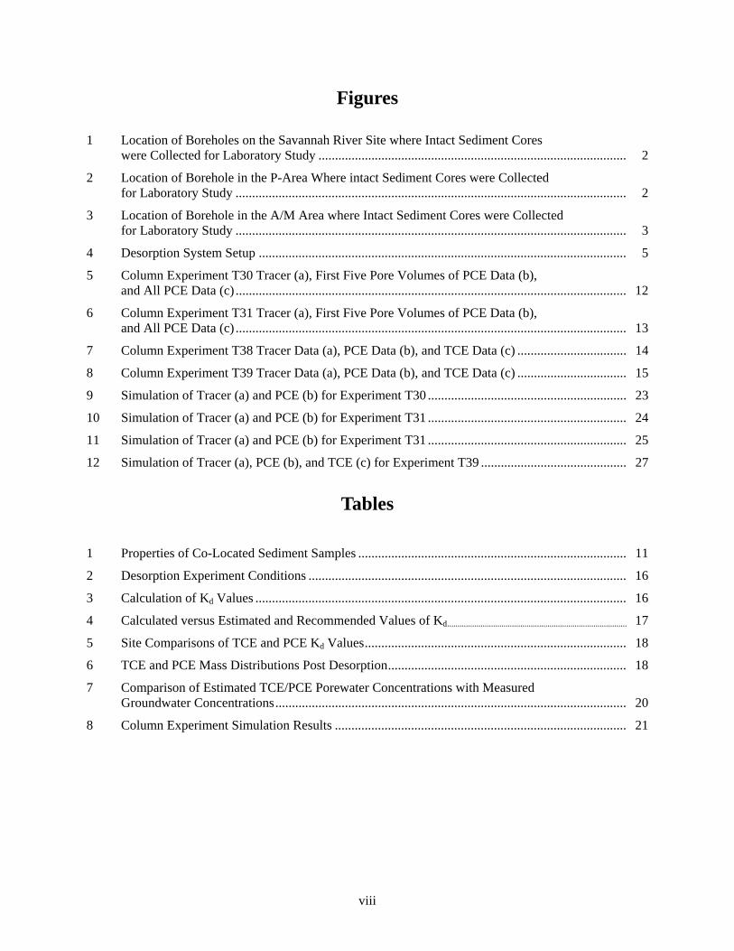
4 Desorption System Setup ............................................................................................................... 5
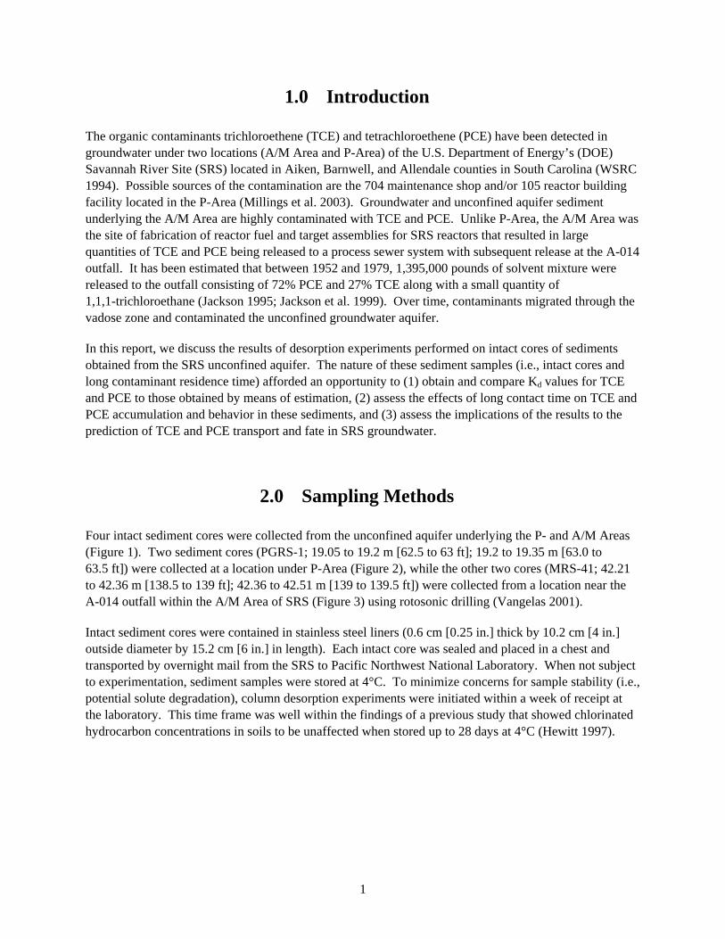
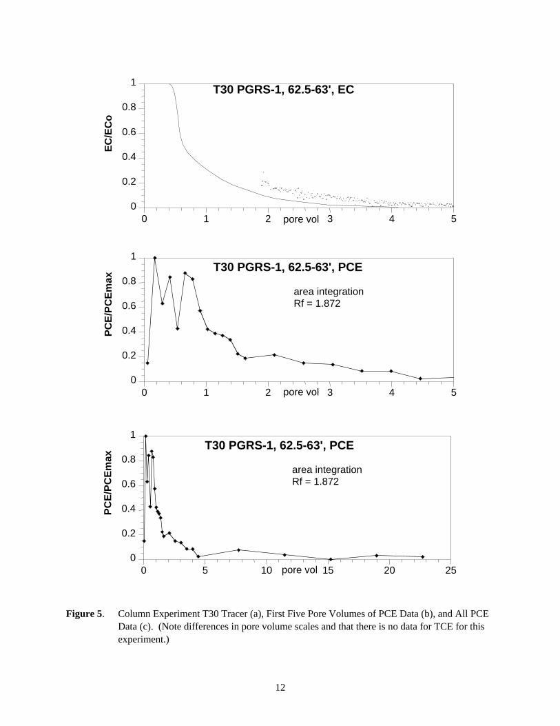
5 Column Experiment T30 Tracer (a), First Five Pore Volumes of PCE Data (b), and All PCE Data (c) ...................................................................................................................... 12
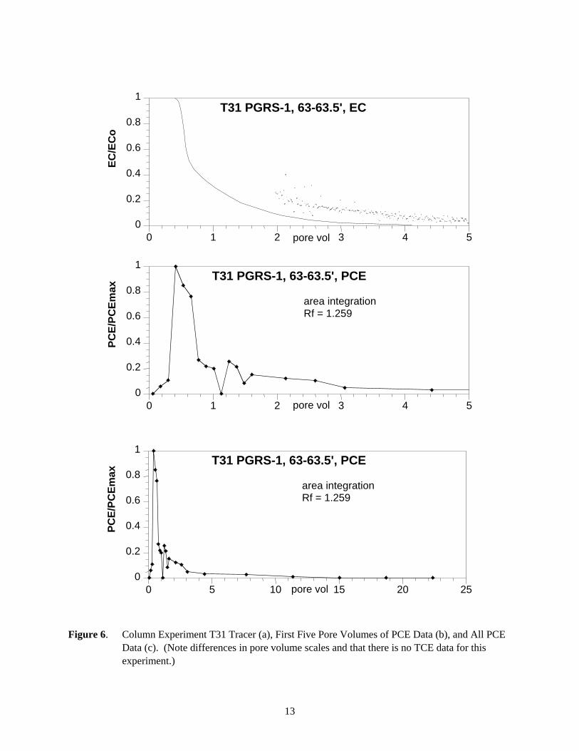
6 Column Experiment T31 Tracer (a), First Five Pore Volumes of PCE Data (b), and All PCE Data (c) ...................................................................................................................... 13
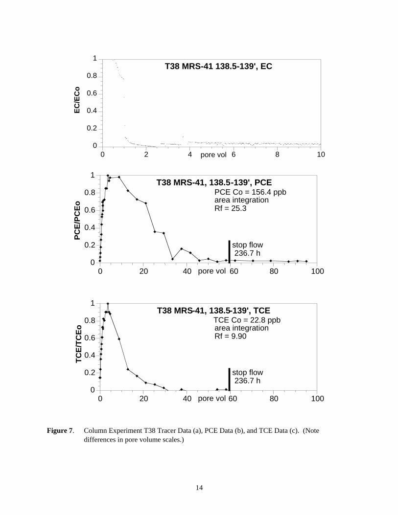
7 Column Experiment T38 Tracer Data (a), PCE Data (b), and TCE Data (c) ................................. 14
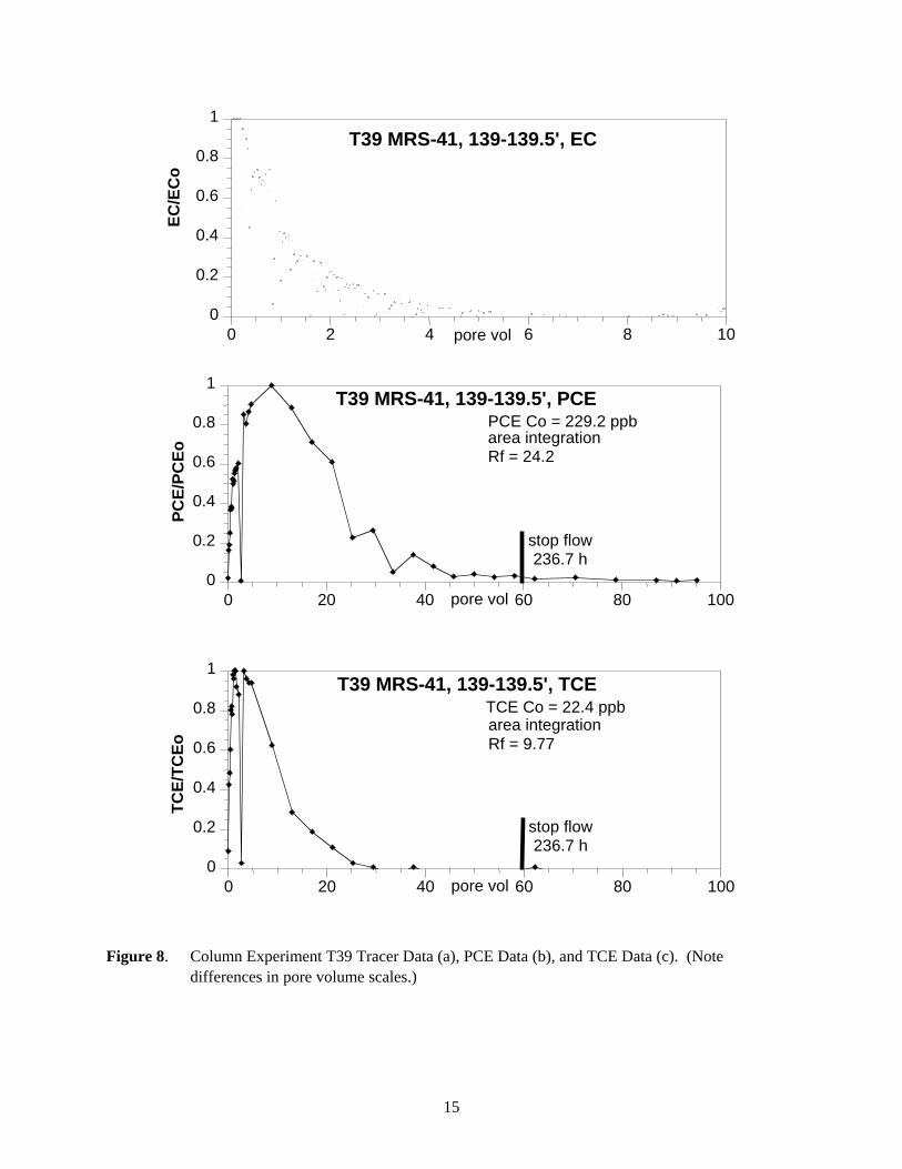
8 Column Experiment T39 Tracer Data (a), PCE Data (b), and TCE Data (c) ................................. 15
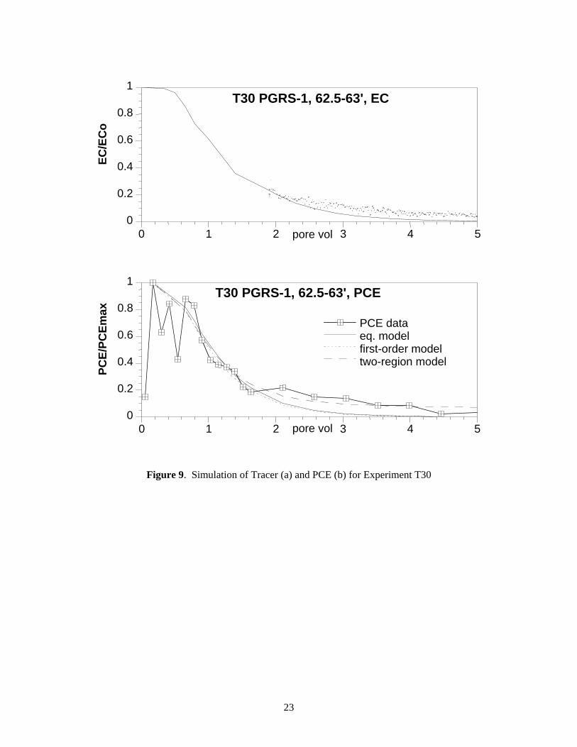
9 Simulation of Tracer (a) and PCE (b) for Experiment T30 ............................................................ 23
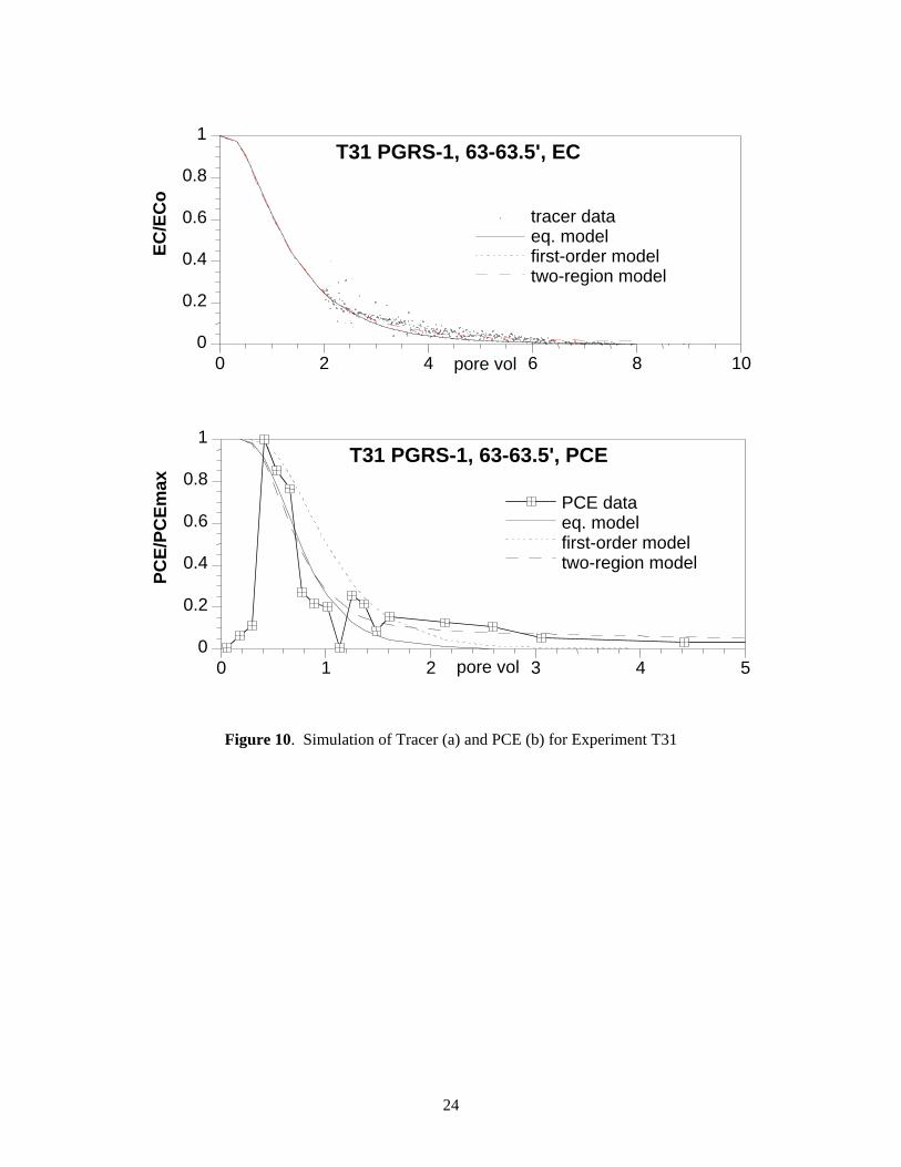
10 Simulation of Tracer (a) and PCE (b) for Experiment T31 ............................................................ 24
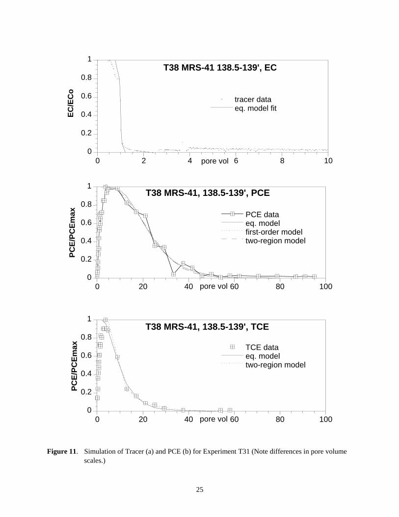
11 Simulation of Tracer (a) and PCE (b) for Experiment T31 ............................................................ 25
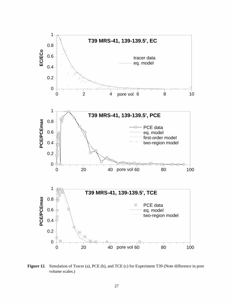
12 Simulation of Tracer (a), PCE (b), and TCE (c) for Experiment T39 ............................................ 27
Tables
1 Properties of Co-Located Sediment Samples ................................................................................. 11
2 Desorption Experiment Conditions ................................................................................................ 16
3 Calculation of Kd Values ................................................................................................................ 16
4 Calculated versus Estimated and Recommended Values of Kd...................................................................................... 17
5 Site Comparisons of TCE and PCE Kd Values............................................................................... 18
6 TCE and PCE Mass Distributions Post Desorption........................................................................ 18
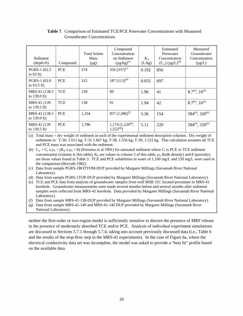
7 Comparison of Estimated TCE/PCE Porewater Concentrations with Measured Groundwater Concentrations.......................................................................................................... 20
8 Column Experiment Simulation Results ........................................................................................ 21
1
1.0 Introduction
The organic contaminants trichloroethene (TCE) and tetrachloroethene (PCE) have been detected in groundwater under two locations (A/M Area and P-Area) of the U.S. Department of Energy’s (DOE) Savannah River Site (SRS) located in Aiken, Barnwell, and Allendale counties in South Carolina (WSRC 1994). Possible sources of the contamination are the 704 maintenance shop and/or 105 reactor building facility located in the P-Area (Millings et al. 2003). Groundwater and unconfined aquifer sediment underlying the A/M Area are highly contaminated with TCE and PCE. Unlike P-Area, the A/M Area was the site of fabrication of reactor fuel and target assemblies for SRS reactors that resulted in large quantities of TCE and PCE being released to a process sewer system with subsequent release at the A-014 outfall. It has been estimated that between 1952 and 1979, 1,395,000 pounds of solvent mixture were released to the outfall consisting of 72% PCE and 27% TCE along with a small quantity of 1,1,1-trichloroethane (Jackson 1995; Jackson et al. 1999). Over time, contaminants migrated through the vadose zone and contaminated the unconfined groundwater aquifer.
In this report, we discuss the results of desorption experiments performed on intact cores of sediments obtained from the SRS unconfined aquifer. The nature of these sediment samples (i.e., intact cores and long contaminant residence time) afforded an opportunity to (1) obtain and compare Kd values for TCE and PCE to those obtained by means of estimation, (2) assess the effects of long contact time on TCE and PCE accumulation and behavior in these sediments, and (3) assess the implications of the results to the prediction of TCE and PCE transport and fate in SRS groundwater.
2.0 Sampling Methods
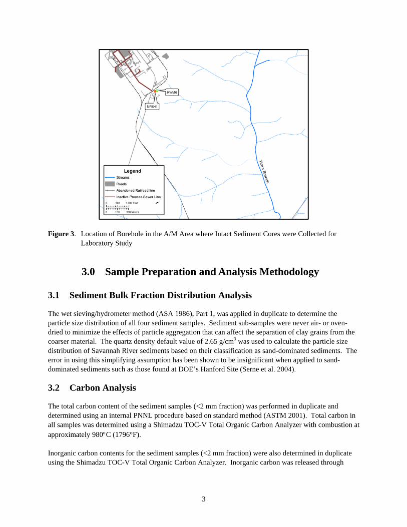
Four intact sediment cores were collected from the unconfined aquifer underlying the P- and A/M Areas (Figure 1). Two sediment cores (PGRS-1; 19.05 to 19.2 m [62.5 to 63 ft]; 19.2 to 19.35 m [63.0 to 63.5 ft]) were collected at a location under P-Area (Figure 2), while the other two cores (MRS-41; 42.21 to 42.36 m [138.5 to 139 ft]; 42.36 to 42.51 m [139 to 139.5 ft]) were collected from a location near the A-014 outfall within the A/M Area of SRS (Figure 3) using rotosonic drilling (Vangelas 2001).
Intact sediment cores were contained in stainless steel liners (0.6 cm [0.25 in.] thick by 10.2 cm [4 in.] outside diameter by 15.2 cm [6 in.] in length). Each intact core was sealed and placed in a chest and transported by overnight mail from the SRS to Pacific Northwest National Laboratory. When not subject to experimentation, sediment samples were stored at 4°C. To minimize concerns for sample stability (i.e., potential solute degradation), column desorption experiments were initiated within a week of receipt at the laboratory. This time frame was well within the findings of a previous study that showed chlorinated hydrocarbon concentrations in soils to be unaffected when stored up to 28 days at 4°C (Hewitt 1997).

2
Figure 1. Location of Boreholes on the Savannah River Site where Intact Sediment Cores were
Collected for Laboratory Study
Figure 2. Location of Borehole in the P-Area Where intact Sediment Cores were Collected for Laboratory Study
3
Figure 3. Location of Borehole in the A/M Area where Intact Sediment Cores were Collected for Laboratory Study
3.0 Sample Preparation and Analysis Methodology
3.1 Sediment Bulk Fraction Distribution Analysis
The wet sieving/hydrometer method (ASA 1986), Part 1, was applied in duplicate to determine the particle size distribution of all four sediment samples. Sediment sub-samples were never air- or oven-dried to minimize the effects of particle aggregation that can affect the separation of clay grains from the coarser material. The quartz density default value of 2.65 g/cm3 was used to calculate the particle size distribution of Savannah River sediments based on their classification as sand-dominated sediments. The error in using this simplifying assumption has been shown to be insignificant when applied to sand-dominated sediments such as those found at DOE’s Hanford Site (Serne et al. 2004).
3.2 Carbon Analysis
The total carbon content of the sediment samples (<2 mm fraction) was performed in duplicate and determined using an internal PNNL procedure based on standard method (ASTM 2001). Total carbon in all samples was determined using a Shimadzu TOC-V Total Organic Carbon Analyzer with combustion at approximately 980°C (1796°F). Inorganic carbon contents for the sediment samples (<2 mm fraction) were also determined in duplicate using the Shimadzu TOC-V Total Organic Carbon Analyzer. Inorganic carbon was released through
4
acid-assisted evolution (50% hydrochloric acid) with heating to 200°C. Organic carbon was calculated as the difference between the measured total and organic carbon.
3.3 Surface Area Analysis
The surface areas of bulk sediments were determined using a combination of nitrogen adsorption BET (Brunauer et al. 1938) and calculation using geometric formulas for the surface area and volume of a sphere. Due to sample size restrictions on the instrumentation (Quantachrome Autosorb-6B; Quantachrome Instruments, Boynton Beach, Florida), only particles less than 2 mm in diameter were measured via BET. The remaining material was sieved into five fractions representing discrete particle diameters: 2.00 to 4.75 mm, 4.75 to 9.5 mm, 9.50 to 19.0 mm, 19.0 to 25.0 mm, and >25.0 mm.
3.4 Experimental Desorption System and Solute Elution
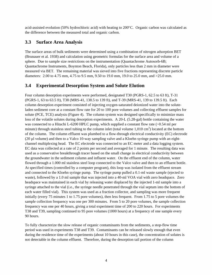
Four column desorption experiments were performed, designated T30 (PGRS-1, 62.5 to 63 ft), T-31 (PGRS-1, 63 to 63.5 ft), T38 (MRS-41, 138.5 to 139 ft), and T-39 (MRS-41, 139 to 139.5 ft). Each column desorption experiment consisted of injecting oxygen-saturated deionized water into the solute-laden sediment core at a constant flow rate for 20 to 100 pore volumes and collecting effluent samples for solute (PCE, TCE) analysis (Figure 4). The column system was designed specifically to minimize mass loss of the volatile solutes during desorption experiments. A 20-L (5.28-gal) bottle containing the water was connected to a Hitachi L-6200 HPLC pump, which supplied a constant flow rate (~0.54 ml per minute) through stainless steel tubing to the column inlet (total volume 1,010 cm3) located at the bottom of the column. The column effluent was plumbed to a flow-through electrical conductivity (EC) electrode (20 µl volume) and then to a Valco 10-way sampling valve and a Kloehn syringe pump with an eight-channel multiplexing head. The EC electrode was connected to an EC meter and a data logging system. EC data was collected at a rate of 2 points per second and averaged for 1 minute. The resulting data was used as a conservative breakthrough tracer based on the small change in electrical conductivity between the groundwater in the sediment column and influent water. On the effluent end of the column, water flowed through a 1.000 ml stainless steel loop connected to the Valco valve and then to an effluent bottle. At specified times (controlled by a computer program), this loop was isolated from the effluent stream and connected to the Kloehn syringe pump. The syringe pump pulled a 0.1-ml waste sample (ejected to waste), followed by a 1.0 ml sample that was injected into a 40-ml VOA vial with zero headspace. Zero headspace was maintained in each vial by releasing water displaced by the injected 1-ml sample into a syringe attached to the vial (i.e., the syringe needle penetrated through the vial septum into the bottom of each water filled vial). This system was used as a fraction collector, and sampling was more frequent initially (every 75 minutes 1 to 1.75 pore volumes), then less frequent. From 1.75 to 5 pore volumes the sample collection frequency was one per 300 minutes. From 5 to 20 pore volumes, the sample collection frequency was one per 40 hours, giving a total experiment time of 200 to 220 hours. For experiments T38 and T39, sampling continued to 95 pore volumes (1000 hours) at a frequency of one sample every 90 hours.
To fully characterize the slow release of organic contaminants from the sediments, a stop-flow time period was used in experiments T38 and T39. Contaminants can be released slowly enough that even during the residence time of the experiments (about 10 hours in this case), the concentration of solutes is not detectable in the column effluent. Therefore, during the desorption tail portion of the column
5
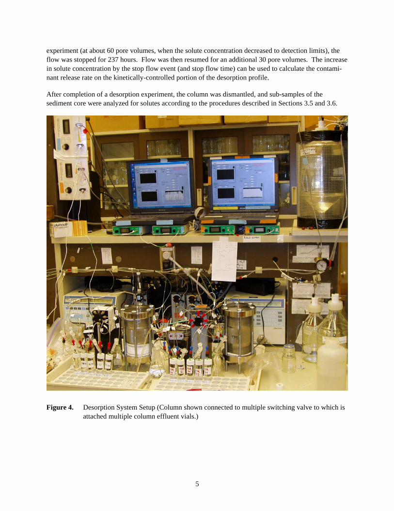
experiment (at about 60 pore volumes, when the solute concentration decreased to detection limits), the flow was stopped for 237 hours. Flow was then resumed for an additional 30 pore volumes. The increase in solute concentration by the stop flow event (and stop flow time) can be used to calculate the contami-nant release rate on the kinetically-controlled portion of the desorption profile.
After completion of a desorption experiment, the column was dismantled, and sub-samples of the sediment core were analyzed for solutes according to the procedures described in Sections 3.5 and 3.6.
Figure 4. Desorption System Setup (Column shown connected to multiple switching valve to which is attached multiple column effluent vials.)
6
3.5 Analysis of Water Samples
Effluent samples from desorption experiments were collected in 40-ml VOA vials. An aliquot of the headspace from the VOA vials was analyzed for TCE and PCE using a Hewlett Packard 5890 gas chromatograph equipped with a HP 5989A mass spectrometer and an OI Analytical 4560 purge and trap system. A capillary column J&W Scientific, DB-624, 75 m, inner diameter (ID) 0.45 mm was used to separate solute compounds. In order to provide optimum sensitivity and selectivity, the selected ion monitoring mode of the mass spectrometer was used. The detection limit for TCE and PCE in water samples was 0.01 µg/L.
3.6 Extraction of Sediments
A DIONEX accelerated solvent extraction system (ASE-200) was used to extract residual TCE and PCE from the post-column desorption experiment sediments using methanol as the extraction solvent. Recovery of aqueous solutions of CCl4 spiked into sediments from previous studies was between 82% and 101% at an optimal temperature of 40°C, depending on the type of soil (Riley et al. 2005). Recovery of TCE and PCE was assumed to be similar to CCl4 (i.e., 82% to 101%) given that TCE and PCE are less volatile than CCl4 (Mackay et al. 1993).
3.7 Analysis of Sediment Extracts by Gas Chromatography and Gas Chromatography/Mass Spectrometry
Methanol extracts of sediments were diluted 50 to 200 times in boiled Milli-Q water and analyzed using a Hewlett Packard 5890 gas chromatograph fitted with a purge and trap system and photoionization and electron capture detectors. TCE and PCE were separated on a 105 m x 0.53 mm megabore capillary column (Restek Corporation) and quantified using a commercial standard (SUPELCO EPA 8260A Calibration Mix) and four-level calibration. The detection limit for TCE and PCE was 0.02 µg/L.
Purge and trap GC/MS was used to analyze samples containing low concentrations of TCE and PCE. Methanol extracts of sediments were diluted 50 times in boiled Milli-Q water and analyzed using a Hewlett Packard 5890 gas chromatograph equipped with a HP 5989A mass spectrometer and an OI Analytical 4560 purge and trap system. A capillary column J&W Scientific, DB-624, 75 m, ID 0.45 mm was used to separate solute compounds. In order to provide optimum sensitivity and selectivity, the selected ion monitoring mode of the mass spectrometer was used.

7
4.0 Data Analysis and Modeling Methods
4.1 Determination of Solute Sorption Parameters from 1-D Column Experiments
Chemical parameters defining the mass of solutes (PCE, TCE) on the sediment surface and the rate of desorption were determined from the one-dimensional (1-D) column breakthrough curves (profiles) by area integration and with an inverse parameter estimation code (CXTFIT, Toride et al. 1993, 1999), as described below. This approach was used to characterize the physical and chemical processes that were occurring in the sediments and yielded solute partition coefficients (Kd values) and kinetic parameters describing slow solute release from sediments. Both physical and chemical processes control the shape of the tracer and solute desorption curve. Idealized 1-D flow of a nonsorbing (conservative) tracer through a homogeneous sediment column defines both a “pore volume” (volume of liquid in the 100% mobile pore space) and the physical breakthrough curve spreading caused by flow through porous media, as defined by the longitudinal hydrodynamic dispersion (DL), as defined by:
DL = Do + αL v (1)
where Do is molecular diffusion, αL is the longitudinal dispersivity, and v is the interstitial velocity. Idealized transport of a sorbing solute in the same homogeneous sediment column will be subject to the same longitudinal dispersion (producing breakthrough curve spreading) but will lag relative to the tracer due to the reversible sorption/desorption (i.e., the overall solute velocity is slower because the solute is sorbed on the surface a portion of the time). The “retardation factor” (Rf) is defined by the ratio of velocities of the tracer/solute so that a value of 1.0 indicates no sorption (solute travels at the same velocity as the tracer) and a value >1.0 indicates sorption. With no additional assumption as to the sorption mechanism or rate, the solute retardation factor can be determined by integrating the area in front of the solute breakthrough curve. The sorption mass parameter Kd is defined by the mass of solute on the sediment surface (per gram of sediment) to the mass of solute in aqueous solution (per mL of solution), and can be calculated from Rf by:
Rf = 1 + ρbKd/θ (2)
where ρb is the dry bulk density (g/cm3) and θ is the total porosity. The dry bulk density was calculated from sediment dry weight and total column volume for each experiment. Column porosity was calculated from values of sediment wet weight and dry weight for each column experiment. In this study, the Kd values were determined by area integration, as described above, which accounts for all of the solute lag in retardation relative to a tracer in both homogeneous and heterogeneous sediments. Model fits to break-through data (equilibrium, first-order, and two-region models) also yielded Kd values, but these were not considered as accurate as area integration, because in some cases the model fit was poor. In general, a poor model fit meant that mathematical description of the physical and chemical processes was insufficient to describe the actual data.
8
4.2 Model Fitting of Breakthrough Curve Data
Reactive transport modeling was used to determine the solute desorption rate from the breakthrough data using the CXTFIT code (Toride et al. 1993, 1999). The CXTFIT code contains analytical solutions to an equilibrium model, a first-order model, and a two-region model. This equilibrium model is defined by the differential Equation (3):
zC v-
zC D
tS b
2
2
L ∂∂
∂∂
=∂∂
θρ (3)
The model includes three parameters; velocity (v), retardation factor, (Rf), and longitudinal dispersion (DL) to describe the rate of change in the solute or tracer aqueous concentration (C) or surface concentration (S), as first described by Gleuckauf (1947). An analytical solution to this model with a nonlinear least squares parameter estimation routine was first described by van Genuchten and others (1974, 1979).
The first-order model, by incorporation of the kinetic reaction (4),
S k
k C
b
f (4)
accounts for reversible slow adsorption and slow desorption where kf is the forward rate coefficient and kb is the backward rate coefficient. An advective-dispersive transport with this single, reversible, linear adsorption/desorption reaction is defined by the solution to the differential Equations (5) and (6):
zC v-
zCD
tS b
tC
2
2
∂∂
∂∂
=∂∂
θρ
+∂∂ (5)
S k - Ck tS bf
b =∂∂
θρ (6)
with previously defined parameters. This first-order model contains four parameters; velocity, longitudinal dispersion, and the two reaction rate parameters (kf, kb). The equilibrium distribution coefficient is by definition kf/kb. The first-order kinetic model was first fit to 1-D solute transport data in sediments by Leenheer and Ahlrichs (1971).
The two-region model describes solute advective/dispersive transport through a porous media with both mobile (subscript “e”) and immobile (subscript “i”) pore regions and equilibrium sorption in both regions (van Genuchten et al. 1974), as defined by the differential Equations (7) and (8):
zC v-
zC D
tS f) - (1
tS f
tC
tC
e2e
2
Li
be
bi
ie
e ∂∂
θ∂
∂=
∂∂
ρ+∂
∂ρ+
∂∂
θ+∂
∂θ (7)
)C - (C t
S f) - (1 t
C ieei
bi
i α=∂
∂ρ+
∂∂
θ (8)
9
where f is the fraction of sorbent in the mobile region, Ce and Ci are solute concentrations in the mobile and immobile regions, respectively; Se and Si are the respective sorbed concentrations, and θe and θi are the volume fractions of the mobile and immobile liquid regions. Mobile pore regions are those regions in where advective transport of pore fluid occurs. Immobile pore regions are those regions in a porous media where pore fluid is trapped (e.g., in media microfactures). This two-region model has five parameters: velocity (v), longitudinal dispersion (DL), equilibrium sorption (Kd = S/C), diffusional mass transfer between mobile and immobile pore fluid (αe), and the fraction of solute mass in the mobile region (f). The two-region model is mathematically equivalent to a fast and slow reaction in parallel or in series.
Model fits to breakthrough data (equilibrium, first-order, and two-region models) were evaluated in the context of three general scenarios:
(i) equilibrium model shows a good fit to both tracer and solute breakthrough data. This indicates an equilibrium adsorption/desorption reaction (Kd = S/C) could explain the observed desorption behavior.
(ii) equilibrium model fit to tracer data, but solute data has a poor fit with the equilibrium model and a good fit with the first-order model. This indicates equilibrium sorption was not the only process occurring, and that reversible first-order kinetics was required to represent observed desorption behavior.
(iii) equilibrium model fit to tracer data, but solute data has a poor fit with the equilibrium and first-order model but a good fit with the two-region model. This indicates that a complex set of either two physical or two chemical processes (i.e., one kinetic and one at equilibrium) are required to represent observed desorption behavior).
Because both hydrodynamic dispersion and slow sorption/desorption will define the solute breakthrough curve shape, a systematic modeling method was used to accurately define these separate processes. In step 1, the equilibrium model was used to fit the tracer data in order to define the hydrodynamic dispersion (longitudinal) with a defined velocity and defined retardation factor (1.0; i.e., the velocity and retardation factor were not allowed to vary in the simulation, only the dispersion). In step 2, the solute data was fit with this equilibrium model with the velocity fixed and longitudinal dispersion fixed at the tracer value (i.e., allowing Rf to vary). If a good fit of the solute data was observed with equilibrium model simulation, then it was concluded that no significant slow release of the solute from the sediment was occurring in the desorption process. For those desorption profiles where additional breakthrough curve spreading was observed (i.e., greater than that defined by longitudinal dispersion), indicating the presence of slow desorption of the solute from the sediment surface, first-order and two-region models were used to fit the solute data to evaluate the nature of the slow desorption process. In these simulations, the longitudinal dispersion was fixed at the value determined by the equilibrium model fit to the tracer data. “Goodness of fit” was described by comparing breakthrough data to model fit (sum of the squares difference between data and model fit at each point) and comparison of the breakthrough area of the actual data to the simulation.
10
5.0 Results
5.1 Physical and Chemical Characteristics of Sediments
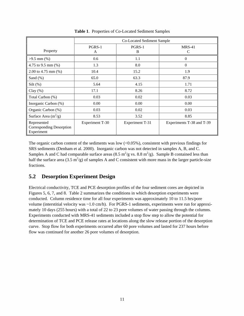
Table 1 summarizes the physical-chemical characteristics of three sediment samples taken adjacent to the sediment cores (i.e., within 15.24 cm [6 in.]) used in the desorption experiments. Properties of these sediments were assumed to be the same as those used in the desorption experiments based on visual comparison of the sediments’ bulk-fraction features. Samples A and B, representing sediments co-located with PGRS-1 intact cores, had similar distributions with approximately 77 to 88% of the mass associated with the gravel and sand fractions. This is in contrast to sediment sample C, representing MRS-41 intact cores which contained a high sand content (87.9%) and virtually no gravel. Silt contents varied between 1.7% and 5.6%, and clay contents varied between 8.3% and 17.1%. The highest silt/clay content was found in sample A.
11
Table 1. Properties of Co-Located Sediment Samples
Co-Located Sediment Sample
Property PGRS-1
A PGRS-1
B MRS-41
C
>9.5 mm (%) 0.6 1.1 0 4.75 to 9.5 mm (%) 1.3 8.0 0 2.00 to 4.75 mm (%) 10.4 15.2 1.9 Sand (%) 65.0 63.3 87.9 Silt (%) 5.64 4.15 1.71 Clay (%) 17.1 8.26 8.72 Total Carbon (%) 0.03 0.02 0.03 Inorganic Carbon (%) 0.00 0.00 0.00 Organic Carbon (%) 0.03 0.02 0.03 Surface Area (m2/g) 8.53 3.52 8.85 Represented Corresponding Desorption Experiment
Experiment T-30 Experiment T-31 Experiments T-38 and T-39
The organic carbon content of the sediments was low (<0.05%), consistent with previous findings for SRS sediments (Denham et al. 2000). Inorganic carbon was not detected in samples A, B, and C. Samples A and C had comparable surface areas (8.5 m2/g vs. 8.8 m2/g). Sample B contained less than half the surface area (3.5 m2/g) of samples A and C consistent with more mass in the larger particle-size fractions.
5.2 Desorption Experiment Design
Electrical conductivity, TCE and PCE desorption profiles of the four sediment cores are depicted in Figures 5, 6, 7, and 8. Table 2 summarizes the conditions in which desorption experiments were conducted. Column residence time for all four experiments was approximately 10 to 11.5 hrs/pore volume (interstitial velocity was ~1.0 cm/h). For PGRS-1 sediments, experiments were run for approxi-mately 10 days (255 hours) with a total of 22 to 23 pore volumes of water passing through the columns. Experiments conducted with MRS-41 sediments included a stop flow step to allow the potential for determination of TCE and PCE release rates at locations along the slow release portion of the desorption curve. Stop flow for both experiments occurred after 60 pore volumes and lasted for 237 hours before flow was continued for another 26 pore volumes of desorption.
12
Figure 5. Column Experiment T30 Tracer (a), First Five Pore Volumes of PCE Data (b), and All PCE Data (c). (Note differences in pore volume scales and that there is no data for TCE for this experiment.)
0
0.2
0.4
0.6
0.8
1
0 1 2 3 4 5
EC/E
Co
pore vol
T30 PGRS-1, 62.5-63', EC
0
0.2
0.4
0.6
0.8
1
0 1 2 3 4 5
PCE/
PCEm
ax
pore vol
T30 PGRS-1, 62.5-63', PCE
area integrationRf = 1.872
0
0.2
0.4
0.6
0.8
1
0 5 10 15 20 25
PCE/
PCEm
ax
pore vol
T30 PGRS-1, 62.5-63', PCE
area integrationRf = 1.872
13
Figure 6. Column Experiment T31 Tracer (a), First Five Pore Volumes of PCE Data (b), and All PCE Data (c). (Note differences in pore volume scales and that there is no TCE data for this experiment.)
0
0.2
0.4
0.6
0.8
1
0 1 2 3 4 5
EC/E
Co
pore vol
T31 PGRS-1, 63-63.5', EC
0
0.2
0.4
0.6
0.8
1
0 1 2 3 4 5
PCE/
PCEm
ax
pore vol
T31 PGRS-1, 63-63.5', PCE
area integrationRf = 1.259
0
0.2
0.4
0.6
0.8
1
0 5 10 15 20 25
PCE/
PCEm
ax
pore vol
T31 PGRS-1, 63-63.5', PCE
area integrationRf = 1.259
14
0
0.2
0.4
0.6
0.8
1
0 2 4 6 8 10
EC/E
Co
pore vol
T38 MRS-41 138.5-139', EC
Figure 7. Column Experiment T38 Tracer Data (a), PCE Data (b), and TCE Data (c). (Note differences in pore volume scales.)
0
0.2
0.4
0.6
0.8
1
0 20 40 60 80 100
TCE/
TCEo
pore vol
T38 MRS-41, 138.5-139', TCE
stop flow236.7 h
TCE Co = 22.8 ppb area integrationRf = 9.90
0
0.2
0.4
0.6
0.8
1
0 20 40 60 80 100
PCE/
PCEo
pore vol
T38 MRS-41, 138.5-139', PCE
stop flow236.7 h
PCE Co = 156.4 ppb area integrationRf = 25.3
15
Figure 8. Column Experiment T39 Tracer Data (a), PCE Data (b), and TCE Data (c). (Note differences in pore volume scales.)
0
0.2
0.4
0.6
0.8
1
0 20 40 60 80 100
PCE/
PCEo
pore vol
stop flow236.7 h
PCE Co = 229.2 ppbarea integrationRf = 24.2
T39 MRS-41, 139-139.5', PCE
0
0.2
0.4
0.6
0.8
1
0 20 40 60 80 100
TCE/
TCEo
pore vol
stop flow236.7 h
TCE Co = 22.4 ppbarea integrationRf = 9.77
T39 MRS-41, 139-139.5', TCE
0
0.2
0.4
0.6
0.8
1
0 2 4 6 8 10
EC/E
Co
pore vol
T39 MRS-41, 139-139.5', EC
16
Table 2. Desorption Experiment Conditions
Sediment/Experiment Flow Rate
(hrs/pore volume) Pore Volumes Length of Desorption (hrs)
PGRS-1 (T-30) 11.24 23 255 PGRS-1 (T-31) 11.47 22 255 MRS-41 (T-38) 10.23 60
36 614(a)
368 MRS-41 (T-39) 10.25 60
36 615(a)
368 (a) After the first 60 pore volumes, flow was stopped for 237 hrs. Flow was then initiated for another 36 pore
volumes.
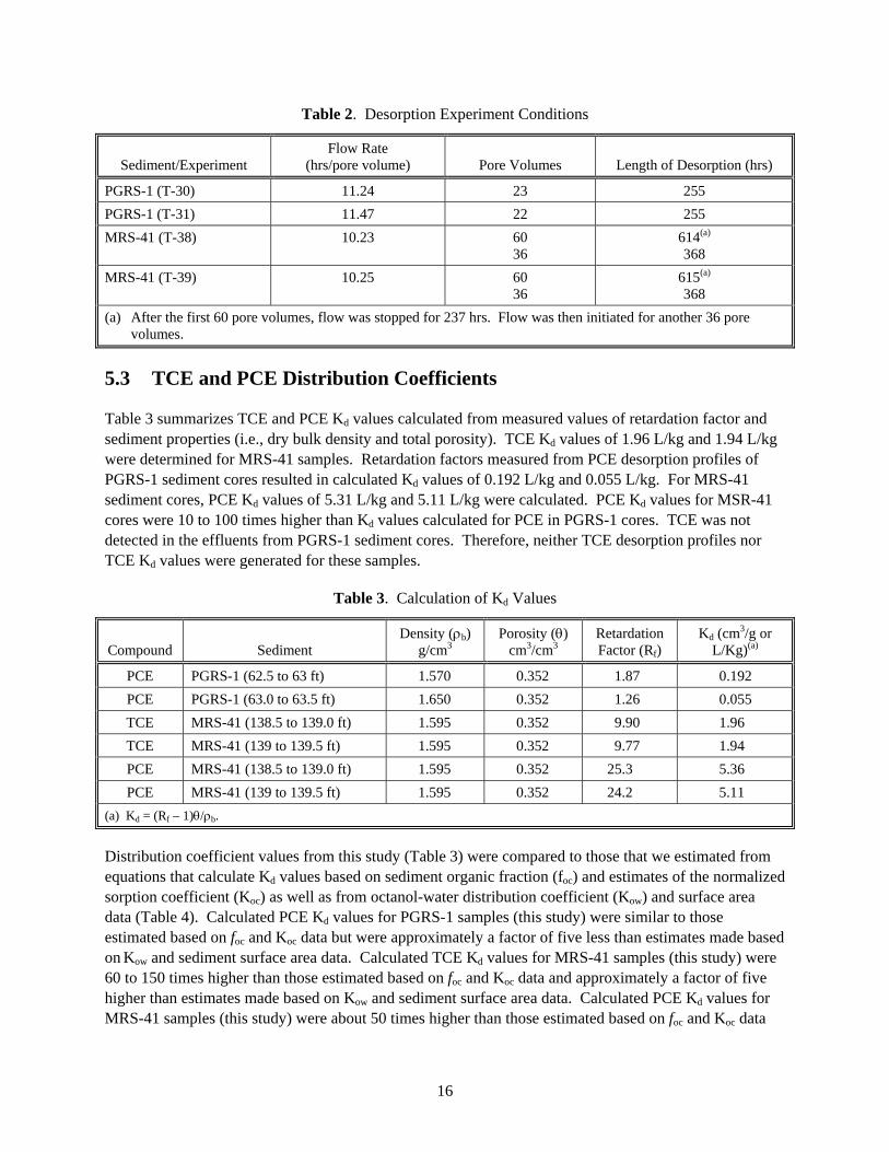
5.3 TCE and PCE Distribution Coefficients
Table 3 summarizes TCE and PCE Kd values calculated from measured values of retardation factor and sediment properties (i.e., dry bulk density and total porosity). TCE Kd values of 1.96 L/kg and 1.94 L/kg were determined for MRS-41 samples. Retardation factors measured from PCE desorption profiles of PGRS-1 sediment cores resulted in calculated Kd values of 0.192 L/kg and 0.055 L/kg. For MRS-41 sediment cores, PCE Kd values of 5.31 L/kg and 5.11 L/kg were calculated. PCE Kd values for MSR-41 cores were 10 to 100 times higher than Kd values calculated for PCE in PGRS-1 cores. TCE was not detected in the effluents from PGRS-1 sediment cores. Therefore, neither TCE desorption profiles nor TCE Kd values were generated for these samples.
Table 3. Calculation of Kd Values
Compound Sediment Density (ρb)
g/cm3 Porosity (θ)
cm3/cm3 Retardation Factor (Rf)
Kd (cm3/g or L/Kg)(a)
PCE PGRS-1 (62.5 to 63 ft) 1.570 0.352 1.87 0.192 PCE PGRS-1 (63.0 to 63.5 ft) 1.650 0.352 1.26 0.055 TCE MRS-41 (138.5 to 139.0 ft) 1.595 0.352 9.90 1.96 TCE MRS-41 (139 to 139.5 ft) 1.595 0.352 9.77 1.94 PCE MRS-41 (138.5 to 139.0 ft) 1.595 0.352 25.3 5.36 PCE MRS-41 (139 to 139.5 ft) 1.595 0.352 24.2 5.11
(a) Kd = (Rf – 1)θ/ρb.
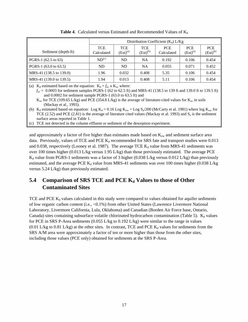
Distribution coefficient values from this study (Table 3) were compared to those that we estimated from equations that calculate Kd values based on sediment organic fraction (foc) and estimates of the normalized sorption coefficient (Koc) as well as from octanol-water distribution coefficient (Kow) and surface area data (Table 4). Calculated PCE Kd values for PGRS-1 samples (this study) were similar to those estimated based on foc and Koc data but were approximately a factor of five less than estimates made based on Kow and sediment surface area data. Calculated TCE Kd values for MRS-41 samples (this study) were 60 to 150 times higher than those estimated based on foc and Koc data and approximately a factor of five higher than estimates made based on Kow and sediment surface area data. Calculated PCE Kd values for MRS-41 samples (this study) were about 50 times higher than those estimated based on foc and Koc data
17
Table 4. Calculated versus Estimated and Recommended Values of Kd
Distribution Coefficient (Kd) L/Kg
Sediment (depth-ft) TCE
Calculated TCE
(Est)(a) TCE
(Est)(b) PCE
Calculated PCE
(Est)(a) PCE
(Est)(b)
PGRS-1 (62.5 to 63) ND(c) ND NA 0.192 0.106 0.454 PGRS-1 (63.0 to 63.5) ND ND NA 0.055 0.071 0.452 MRS-41 (138.5 to 139.0) 1.96 0.032 0.408 5.35 0.106 0.454 MRS-41 (139.0 to 139.5) 1.94 0.013 0.408 5.11 0.106 0.454 (a) Kd estimated based on the equation: Kd = foc x Koc where:
foc = 0.0003 for sediment samples PGRS-1 (62 to 62.5 ft) and MRS-41 (138.5 to 139 ft and 139.0 ft to 139.5 ft) and 0.0002 for sediment sample PGRS-1 (63.0 to 63.5 ft) and
Koc for TCE (109.65 L/kg) and PCE (354.8 L/kg) is the average of literature-cited values for Koc in soils (Mackay et al., 1993).
(b) Kd estimated based on equation: Log Kd = 0.16 Log Kow + Log Sa/200 (McCarty et al. 1981) where log Kow for TCE (2.52) and PCE (2.81) is the average of literature cited values (Mackay et al. 1993) and Sa is the sediment surface areas reported in Table 1.
(c) TCE not detected in the column effluent or sediment of the desorption experiment.
and approximately a factor of five higher than estimates made based on Kow and sediment surface area data. Previously, values of TCE and PCE Kd recommended for SRS fate and transport studies were 0.013 and 0.038, respectively (Looney et al. 1987). The average TCE Kd value from MRS-41 sediments was over 100 times higher (0.013 L/kg versus 1.95 L/kg) than those previously estimated. The average PCE Kd value from PGRS-1 sediments was a factor of 3 higher (0.038 L/kg versus 0.012 L/kg) than previously estimated, and the average PCE Kd value from MRS-41 sediments was over 100 times higher (0.038 L/kg versus 5.24 L/kg) than previously estimated.
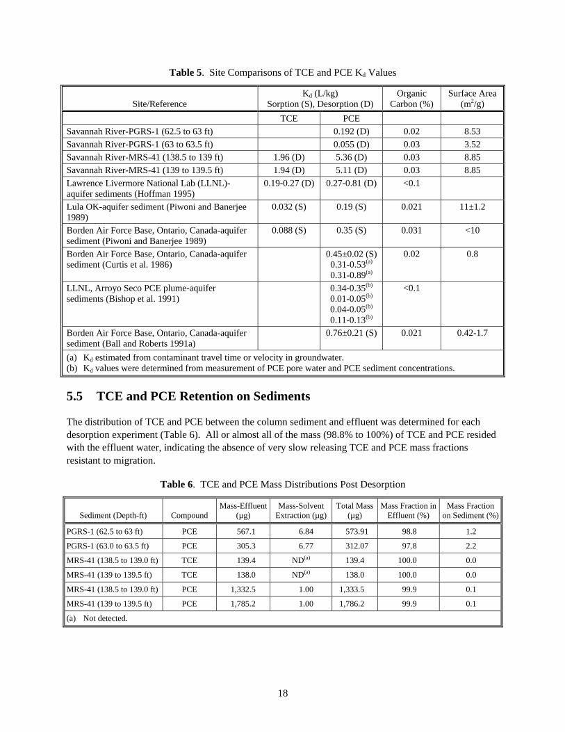
5.4 Comparison of SRS TCE and PCE Kd Values to those of Other Contaminated Sites
TCE and PCE Kd values calculated in this study were compared to values obtained for aquifer sediments of low organic carbon content (i.e., <0.1%) from other United States (Lawrence Livermore National Laboratory, Livermore California, Lula, Oklahoma) and Canadian (Borden Air Force base, Ontario, Canada) sites containing subsurface volatile chlorinated hydrocarbon contamination (Table 5). Kd values for PCE in SRS P-Area sediments (0.055 L/kg to 0.192 L/kg) were similar to the range in values (0.01 L/kg to 0.81 L/kg) at the other sites. In contrast, TCE and PCE Kd values for sediments from the SRS A/M area were approximately a factor of ten or more higher than those from the other sites, including those values (PCE only) obtained for sediments at the SRS P-Area.
18
Table 5. Site Comparisons of TCE and PCE Kd Values
Site/Reference Kd (L/kg)
Sorption (S), Desorption (D) Organic
Carbon (%) Surface Area
(m2/g) TCE PCE Savannah River-PGRS-1 (62.5 to 63 ft) 0.192 (D) 0.02 8.53 Savannah River-PGRS-1 (63 to 63.5 ft) 0.055 (D) 0.03 3.52 Savannah River-MRS-41 (138.5 to 139 ft) 1.96 (D) 5.36 (D) 0.03 8.85 Savannah River-MRS-41 (139 to 139.5 ft) 1.94 (D) 5.11 (D) 0.03 8.85 Lawrence Livermore National Lab (LLNL)-aquifer sediments (Hoffman 1995)
0.19-0.27 (D) 0.27-0.81 (D) <0.1
Lula OK-aquifer sediment (Piwoni and Banerjee 1989)
0.032 (S) 0.19 (S) 0.021 11±1.2
Borden Air Force Base, Ontario, Canada-aquifer sediment (Piwoni and Banerjee 1989)
0.088 (S) 0.35 (S) 0.031 <10
Borden Air Force Base, Ontario, Canada-aquifer sediment (Curtis et al. 1986)
0.45±0.02 (S)0.31-0.53(a) 0.31-0.89(a)
0.02 0.8
LLNL, Arroyo Seco PCE plume-aquifer sediments (Bishop et al. 1991)
0.34-0.35(b) 0.01-0.05(b) 0.04-0.05(b) 0.11-0.13(b)
<0.1
Borden Air Force Base, Ontario, Canada-aquifer sediment (Ball and Roberts 1991a)
0.76±0.21 (S) 0.021 0.42-1.7
(a) Kd estimated from contaminant travel time or velocity in groundwater. (b) Kd values were determined from measurement of PCE pore water and PCE sediment concentrations.
5.5 TCE and PCE Retention on Sediments
The distribution of TCE and PCE between the column sediment and effluent was determined for each desorption experiment (Table 6). All or almost all of the mass (98.8% to 100%) of TCE and PCE resided with the effluent water, indicating the absence of very slow releasing TCE and PCE mass fractions resistant to migration.
Table 6. TCE and PCE Mass Distributions Post Desorption
Sediment (Depth-ft) Compound Mass-Effluent
(µg) Mass-Solvent
Extraction (µg) Total Mass
(µg) Mass Fraction in
Effluent (%) Mass Fraction
on Sediment (%)
PGRS-1 (62.5 to 63 ft) PCE 567.1 6.84 573.91 98.8 1.2
PGRS-1 (63.0 to 63.5 ft) PCE 305.3 6.77 312.07 97.8 2.2
MRS-41 (138.5 to 139.0 ft) TCE 139.4 ND(a) 139.4 100.0 0.0
MRS-41 (139 to 139.5 ft) TCE 138.0 ND(a) 138.0 100.0 0.0
MRS-41 (138.5 to 139.0 ft) PCE 1,332.5 1.00 1,333.5 99.9 0.1
MRS-41 (139 to 139.5 ft) PCE 1,785.2 1.00 1,786.2 99.9 0.1
(a) Not detected.
19
5.6 Sediment DNAPL and Porewater Concentration Assessments
Total TCE and PCE masses in the column desorption experiments (Table 6, column 5) were used to calculate maximum TCE and PCE sediment concentrations present in each sediment core prior to conducting the desorption experiments. Calculated concentrations showed good agreement with PCE concentration in co-located samples collected and analyzed independently by staff at the Savannah River National Laboratory (Table 7). Sediment concentrations were used to calculate sediment porewater concentrations as a basis for assessing whether a TCE or PCE DNAPL phase may have been present in the sediment cores prior to conduct of the sediment desorption experiments (Feenstra et al. 1991). The presence of DNAPL would confound the interpretation of the desorption Kd results if dissolution from a DNAPL phase was occurring during aqueous desorption. In all cases, porewater concentrations were significantly below TCE and PCE concentrations necessary to exceed TCE and PCE solubility in water, indicating the absence of TCE and/or PCE DNAPL in the sediments (Table 7). Estimated porewater concentration of TCE and PCE in MRS-41 sediments was compared to the concentration of TCE and PCE measured in groundwater from well MSB 31C located proximate to sediment sample collection. Groundwater data were from samples collected at about the same time of sediment sample collection (i.e., groundwater samples were collected in September 2005 and March 2006 and the sediment samples were collected in January 2006). There was good agreement between estimated porewater concentration and groundwater concentration for both TCE and PCE (i.e., concentrations were within a factor of approxi-mately 2 to 3 of each other). Note that the high values of Kd for TCE and PCE are necessary for reasonable comparability with measured groundwater concentrations.
5.7 Breakthrough Curve Analysis
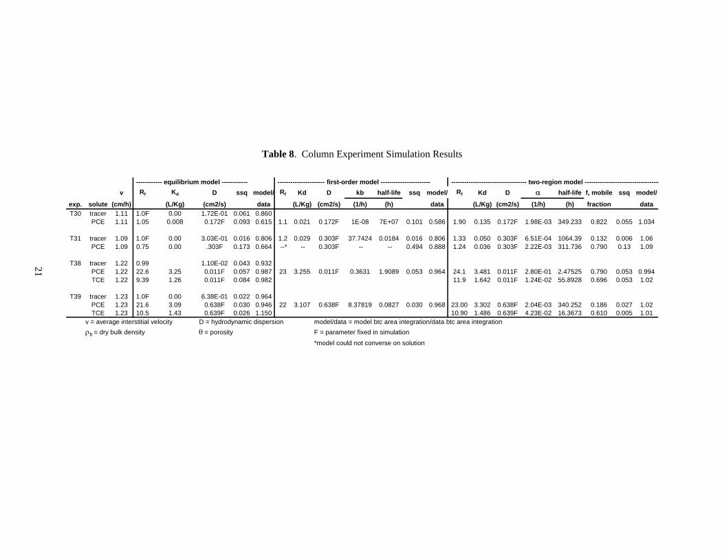
Table 8 summarizes parameter data for equilibrium, first-order, and two-region model simulations of the TCE and PCE desorption profiles from the four sediments from the two SRS sampling sites. Simulated profiles from application of equilibrium, first-order, and two- region models to tracer, TCE, and PCE data were used to assess TCE and PCE desorption behavior in PGRS-1 and MRS-41 sediments. One possibility is that TCE and PCE desorption from sediments can be explained with only the mechanisms of advective-dispersive transport (i.e., the application of a simple equilibrium model), indicating reversible sorption as the process governing their migration in SRS sediment. Another possibility is that desorption is kinetically-controlled. The simplest kinetic reaction is first-order reversible sorption (sorption to a single site), and its application in a transport model uses the sorption and desorption rate. A model that incorporates equilibrium sorption parallel to first-order kinetic sorption (two-region model) was also used to describe breakthrough curve shape. An improved fit with the first-order or second-order models over the equilibrium model suggests (but does not prove) that TCE and PCE migration is a function of some combination of reversible and irreversible sorption processes.
For the purposes of our analyses, irreversible processes are of two types. In type 1, TCE and PCE absorption into the sediment has been moderate in which case desorption behavior may be explained with a first-order model or two-region model with reversible sorption remaining the dominant process. In type 2, a significant source of TCE and/or PCE mass as a migration resistant fraction (MRF) is found remaining in the sediment after desorption. This MRF releases TCE or PCE very slowly into the migrating pore water. We assume the release rate of TCE or PCE from MRF is orders of magnitude slower than the release rate for moderately absorbed TCE and/or PCE. In this case, we assume that
20
Table 7. Comparison of Estimated TCE/PCE Porewater Concentrations with Measured Groundwater Concentrations
Sediment (depth-ft) Compound
Total Solute Mass (µg)
Compound Concentration on Sediment
(µg/kg)(a) Kd
(L/kg)
Estimated Porewater
Concentration (Cw) (µg/L)(b)
Measured Groundwater Concentration
(µg/L)
PGRS-1 (62.5 to 63 ft)
PCE 574 356 (337)(c) 0.192 856
PGRS-1 (63.0 to 63.5 ft)
PCE 312 187 (113)(d) 0.055 697
MRS-41 (138.5 to 139.0 ft)
TCE 139 89 1.96 41 8.7(e), 16(e)
MRS-41 (139 to 139.5 ft)
TCE 138 91 1.94 42 8.7(e), 16(e)
MRS-41 (138.5 to 139.0 ft)
PCE 1,334 857 (1,086)(f) 5.36 154 584(e), 320(e)
MRS-41 (139 to 139.5 ft)
PCE 1,786 1,174 (1,220(g), 1,553(g))
5.11 220 584(e), 320(e)
(a) Total mass ÷ dry weight of sediment in each of the experimental sediment desorption columns. Dry weight of sediments is: T-30, 1.611 kg; T-31 1.667 kg; T-38, 1.556 kg; T-39, 1.522 kg. This calculation assumes all TCE and PCE mass was associated with the sediment.
(b) Cw = Ct x ρb ÷ (Kd x ρb + θ) (Feenstra et al 1991) for saturated sediment where Ct is PCE or TCE sediment concentration (column 4, this table), Kd are values in column 5 of this table, ρb (bulk density) and θ (porosity) are those values found in Table 3. TCE and PCE solubilities in water of 1,100 mg/L and 150 mg/L were used in the comparison (Horvath 1982).
(c) Data from sample PGRS-1BOTTOM-DUP provided by Margaret Millings (Savannah River National Laboratory).
(d) Data from sample PGRS-1TOP-DUP provided by Margaret Millings (Savannah River National Laboratory). (e) TCE and PCE data from analysis of groundwater samples from well MSB 31C located proximate to MRS-41
borehole. Groundwater measurements were made several months before and several months after sediment samples were collected from MRS-41 borehole. Data provided by Margaret Millings (Savannah River National Laboratory).
(f) Data from sample MRS-41-138-DUP provided by Margaret Millings (Savannah River National Laboratory). (g) Data from sample MRS-41-140 and MRS-41-140 DUP provided by Margaret Millings (Savannah River
National Laboratory).
neither the first-order or two-region model is sufficiently sensitive to discern the presence of MRF release in the presence of moderately absorbed TCE and/or PCE. Analysis of individual experiment simulations are discussed in Sections 5.7.1 through 5.7.4, taking into account previously discussed data (i.e., Table 6 and the results of the stop-flow step in the MRS-41 experiments). In the case of Figure 6a, where the electrical conductivity data set was incomplete, the model was asked to provide a “best fit” profile based on the available data.
21
Table 8. Column Experiment Simulation Results
------------ equilibrium model ------------ ---------------------- first-order model ----------------------- ----------------------------------- two-region model -----------------------------------v Rf Kd D ssq model/ Rf Kd D kb half-life ssq model/ Rf Kd D α half-life f, mobile ssq model/
exp. solute (cm/h) (L/Kg) (cm2/s) data (L/Kg) (cm2/s) (1/h) (h) data (L/Kg) (cm2/s) (1/h) (h) fraction dataT30 tracer 1.11 1.0F 0.00 1.72E-01 0.061 0.860
PCE 1.11 1.05 0.008 0.172F 0.093 0.615 1.1 0.021 0.172F 1E-08 7E+07 0.101 0.586 1.90 0.135 0.172F 1.98E-03 349.233 0.822 0.055 1.034
T31 tracer 1.09 1.0F 0.00 3.03E-01 0.016 0.806 1.2 0.029 0.303F 37.7424 0.0184 0.016 0.806 1.33 0.050 0.303F 6.51E-04 1064.39 0.132 0.006 1.06PCE 1.09 0.75 0.00 .303F 0.173 0.664 --* -- 0.303F -- -- 0.494 0.888 1.24 0.036 0.303F 2.22E-03 311.736 0.790 0.13 1.09
T38 tracer 1.22 0.99 1.10E-02 0.043 0.932
PCE 1.22 22.6 3.25 0.011F 0.057 0.987 23 3.255 0.011F 0.3631 1.9089 0.053 0.964 24.1 3.481 0.011F 2.80E-01 2.47525 0.790 0.053 0.994TCE 1.22 9.39 1.26 0.011F 0.084 0.982 11.9 1.642 0.011F 1.24E-02 55.8928 0.696 0.053 1.02
T39 tracer 1.23 1.0F 0.00 6.38E-01 0.022 0.964
PCE 1.23 21.6 3.09 0.638F 0.030 0.946 22 3.107 0.638F 8.37819 0.0827 0.030 0.968 23.00 3.302 0.638F 2.04E-03 340.252 0.186 0.027 1.02TCE 1.23 10.5 1.43 0.639F 0.026 1.150 10.90 1.486 0.639F 4.23E-02 16.3673 0.610 0.005 1.01
v = average interstitial velocity D = hydrodynamic dispersion model/data = model btc area integration/data btc area integrationρb = dry bulk density θ = porosity F = parameter fixed in simulation *model could not converse on solution
22
5.7.1 Experiment T30 (PGRS-1, 62.5 ft to 63 ft) Simulations
PCE elution in column experiment T30 (Figure 5c) showed a considerable amount of tailing (to 12 pore volumes) beyond the average PCE breakthrough of 1.87 pore volumes. Some of this tailing is accounted for in hydrodynamic dispersion as indicated by the breakthrough curve tailing to 5+ pore volumes (Figure 9a). An equilibrium model was able to account for most of the tailing observed in the tracer data (line in Figure 9a). The tracer dispersivity was adopted as the PCE dispersivity (i.e., the dispersivity value was fixed for PCE simulations so that the PCE desorption processes contribution within the total tailing in the PCE breakthrough curve could be identified). The equilibrium model when applied to the PCE data (solid line, Figure 9b) accounted for only 65% of PCE breakthrough mass (missing the 35% in the tailing), indicating that the simplified process of equilibrium adsorption with dispersion does not account for all of the observed data. The additional tailing could be matched with the two-region model with a small fraction (18%) of PCE slow release sites (desorption half life 350 hours, Table 8). This type of simulation does not prove the existence of a slow release process – the modeling only indicates the breakthrough data can be matched with most solute being transported with reversible adsorption with a small PCE fraction migrating according to a slow release process.
5.7.2 Experiment T31 (PGRS-1, 63 ft to 63.5 ft) Simulations
The PCE elution profile in column experiment T31 (Figure 6c) showed some tailing (up to 8 pore volumes) relative to the average tracer breakthrough of 1.26 pore volumes. Again, the equilibrium model could only account for 66% of the PCE breakthrough mass. Similar to experiment T30 results, the two-region model was best able to fit the PCE data (i.e., it could account for the PCE breakthrough curve tailing) with a small fraction of (21%) of slow PCE release sites (Figure 10a, 10b) (desorption half life 311 hours, Table 8).
5.7.3 Experiment T38 (MRS-41, 138.5 ft to 139 ft) Simulations
PCE and TCE breakthrough data in experiment T38 showed significantly different release behavior as compared to observed desorption behavior in PGRS-1 sediment cores. The tracer data (Figure 11a) showed very little tailing and was well simulated with the equilibrium model. The PCE (Figure 11b) and TCE (Figure 11c) data also were well described by the equilibrium model, in which TCE and PCE concentrations decreased within another 20 pore volumes of the average breakthrough. Application of the first-order and two-region models did not significantly improve the fit. The 237 hours stop flow (Figure 7b, 7c) event at 60 pore volumes yielded no increase in PCE or TCE concentration in the effluent, indicating the absence of measurable TCE and PCE slow release from any TCE and PCE remaining on the sediment. This was affirmed from the fact that no residual TCE or PCE mass was detected on the sediment after desorption. These results indicate that the irreversible sorption process was not significant in this sediment.
23
Figure 9. Simulation of Tracer (a) and PCE (b) for Experiment T30
0
0.2
0.4
0.6
0.8
1
0 1 2 3 4 5
EC/E
Co
pore vol
T30 PGRS-1, 62.5-63', EC
0
0.2
0.4
0.6
0.8
1
0 1 2 3 4 5
PCEneqfotr
PCE/
PCEm
ax
pore vol
T30 PGRS-1, 62.5-63', PCE
PCE data eq. modelfirst-order model two-region model
24
Figure 10. Simulation of Tracer (a) and PCE (b) for Experiment T31
0
0.2
0.4
0.6
0.8
1
0 2 4 6 8 10
T31ecneq mfo mtr
EC/E
Co
pore vol
T31 PGRS-1, 63-63.5', EC
tracer dataeq. modelfirst-order model two-region model
0
0.2
0.4
0.6
0.8
1
0 1 2 3 4 5
PCEneqfotr
PCE/
PCEm
ax
pore vol
PCE data eq. modelfirst-order model two-region model
T31 PGRS-1, 63-63.5', PCE
25
0
0.2
0.4
0.6
0.8
1
0 2 4 6 8 10
ECnH
EC/E
Co
pore vol
T38 MRS-41 138.5-139', EC
tracer dataeq. model fit
Figure 11. Simulation of Tracer (a) and PCE (b) for Experiment T31 (Note differences in pore volume scales.)
0
0.2
0.4
0.6
0.8
1
0 20 40 60 80 100
PCEneqfotr
pore vol
PCE dataeq. modelfirst-order model two-region model
T38 MRS-41, 138.5-139', PCE
PCE/
PCEm
ax
0
0.2
0.4
0.6
0.8
1
0 20 40 60 80 100
TCEneqtr
PCE/
PCEm
ax
pore vol
TCE dataeq. modeltwo-region model
T38 MRS-41, 138.5-139', TCE
26
5.7.4 Experiment 39 (MRS-41, 139 ft to 139.5 ft) Simulations
PCE and TCE breakthrough data in experiment T39 showed essentially the same behavior as the MRS-41 sediment core from experiment T-38. The tracer data (Figure 12a) showed very little tailing and was well simulated with the equilibrium model. The PCE (Figure 12b) and TCE (Figure 12c) data also were well described by the equilibrium model, in which TCE and PCE concentrations decreased within another 20 pore volumes of the average breakthrough. Application of the first-order and two-region models did not significantly improve the fit. The 267 hours stop flow (Figure 8b, 8c) event at 60 pore volumes yielded no increase in PCE or TCE concentration in the effluent, indicating the absence of measurable TCE and PCE slow release from any TCE and PCE remaining on the sediment. This was affirmed from the fact that only trace levels TCE or PCE mass (e.g., PCE mass on sediment was 1 mg on the sediment versus 1,785.2 mg released in the effluent) was detected on the sediment after desorption. These results suggest that the irreversible sorption process was not significant in this sediment.
27
Figure 12. Simulation of Tracer (a), PCE (b), and TCE (c) for Experiment T39 (Note difference in pore volume scales.)
0
0.2
0.4
0.6
0.8
1
0 2 4 6 8 10
ECneqEC
/EC
o
pore vol
T39 MRS-41, 139-139.5', EC
tracer dataeq. model
0
0.2
0.4
0.6
0.8
1
0 20 40 60 80 100
PCEneqfotr
PCE/
PCEm
ax
pore vol
PCE dataeq. modelfirst-order model two-region model
T39 MRS-41, 139-139.5', PCE
0
0.2
0.4
0.6
0.8
1
0 20 40 60 80 100
TCEneqtr
PCE/
PCEm
ax
pore vol
PCE dataeq. modeltwo-region model
T39 MRS-41, 139-139.5', TCE

28
6.0 Discussion
This study produced the first values of TCE and PCE desorption Kds based on measurements of TCE and PCE retardation factors in SRS contaminated aquifer sediments. TCE and PCE had been in contact with these sediments for decades. Such contact times are impractible to reproduce in laboratory experiments. Values of TCE and PCE Kd calculated from measured retardation factors were 1.95 ± 0.01 L/kg (n=2) and 5.24 ± 0.13 L/kg (n=2), respectively for sediments from the A/M Area site. A Kd value of 0.12 ± 0.07 L/kg (n=2) was calculated for PCE in sediments from the P-Area site. Qualitatively, there was a positive correlation between the magnitude of Kd and clay content (i.e., the sediment with higher clay content showed the higher value of Kd). Concentrations of PCE and TCE in the sediments were well below the concentration that would indicate the potential presence of DNAPL, eliminating the presence of DNAPL dissolution as a process that could confound the Kd results. PCE Kd values differed significantly between the two sites, with the PCE Kd value at the A/M Area more than a factor of ten higher then that calculated at the P-Area site. Likewise, values of PCE and TCE Kd at the A/M site were significantly higher than have been reported for other low organic carbon and low surface area aquifer sediments at other contaminated sites in the United States and Canada. An explanation for these differences is unknown at this time (i.e., the lack of significant differences in organic carbon content and clay content of A/M versus P-Area sediments cannot account for these differences in Kd values). However, the results while limited, suggest the need to consider that sorption capacity may play a more important role in mass balance at SRS and that, the A/M Area may take longer to remediate. Estimated porewater concentrations of TCE and PCE in MRS-41 intact core sediments based on the high values of Kd compared reasonably well with concentrations of TCE and PCE measured in samples of groundwater from a well proximate to the site of sediment collection. This helps validate the higher than expected values of Kd determined for TCE and PCE from the desorption experiments.
Kd values of TCE and PCE estimated from sediment organic carbon content and organic carbon distribution coefficients (Koc) or surface area and octanol-water distribution coefficients (Kow) tended to underestimate those that were derived from experimental measurements of retardation factors from this study. Values of TCE and PCE Kd’s were also underestimated when a foc value of 0.01 and literature values of Koc was used in calculating TCE (0.013 L/kg) and PCE (0.038 L/kg) Kds (Looney et al. 1987). This suggests the need to consider, where possible, the acquisition and use of site-specific experimentally-derived data as opposed to data derived from estimation methods as a source of data for tools used in site assessments. Caution should be exercised in applying Kds derived from estimation methods in software tools addressing questions in the context of natural attenuation (e.g., time to remediate) (Chapelle et al. 2003), monitored natural attenuation assessment (e.g., MNAtoolbox- Brady et al. 1999) or numerical models (e.g., RT3D) that incorporate key monitored natural attenuation/enhanced attenuation processes (Clement 1997; Clement et al. 1998).
Values of TCE and PCE Kd in aquifer sediments from previously reported studies have been shown to be greater than those estimated from key parameters (i.e., foc, Koc), consistent with the findings of this study (Ball and Roberts 1991; Curtis et al. 1986; Piwoni and Banerjee 1989). Most significantly, the high TCE and PCE Kd values calculated based on experimental measurement of retardation factors for A/M Area sediments suggests a need to be aware of the possibility of underestimation of the time required for remediation of these sediments based on use of estimated values of Kd or values that have been historically recommended (Looney et al. 1987). For example, previous work has shown that cleanup time (i.e., using pump-and-treat) is approximately 10 times longer for Kd = 1 than the non-reactive case (i.e.,
29
where Kd = 0), and has additional impact for Kd increases up to a value of 5 (Berglund and Cvetkovic 1995). A/M sediments may become a secondary source of TCE and PCE release to groundwater in adjacent sediments of higher permeability (Bear et al. 1994).
All of the TCE and PCE mass (100%) from desorption of sediments from the A/M Area site (MRS-41) was found to be present in the effluent, providing evidence for the absence of TCE or PCE migration resistant fractions in these sediments. Simulation of the experimental tracer and PCE breakthrough curve data showed a good fit with an equilibrium model, consistent with reversible sorption influencing TCE and PCE transport in these sediments. Coupled with the mass distribution data, this suggests the absence of influence of a significant irreversible sorption process. Subsequent to the stop flow component of the MRS-41 experiments, neither TCE or PCE was detected in effluent following resumption of desorption providing further evidence for the absence of migration resistant fractions in these sediments.
In contrast, solute desorption from the two PGRS-1 sediment cores showed some profile tailing in both experiments, indicative of slow release of PCE. Simulation of PCE breakthrough curve data with an equilibrium model could not match the profile tailing observed, and accounted for only 66% of PCE breakthrough mass. Also, a first-order model could not match the tailing behavior observed in the profile. The two region model was able to fit the observed breakthrough data, consistent with the hypothesis that some PCE mass was being released at a moderately slow rate from sediments to solution (irreversible sorption) but not from a significant source of mass remaining in the sediment as a migration resistant fraction. One interpretation of the two-region model results is that most PCE (80%) is being rapidly released from the sediment and a small fraction of PCE (20%) is being slowly released (desorption half-life 320 h). This two sorption site representation could account for the fast desorption of the bulk of PCE mass (66%) and also the slow desorption of the remaining (34%) PCE mass in the tailing portion of the profile. Slow desorption could be chemical in nature (i.e., rate controlled by an actual solute-surface phase chemical reaction) or physical (i.e., slow diffusion out of sediment microfractures, for example).
Sediment samples from the SRS P-Area contained significantly higher percentages of particles in the greater than 2-mm-size range as compared to SRS sediment from the A/M area (12.3% and 24.3% versus 1.9%). Previous work has shown the coarse grain fractions of low organic carbon aquifer sediments sorb PCE (Ball and Roberts 1991) and other chlorinated hydrocarbon compounds (Zhao et al. 2005) to an extent that was disproportionate to its mass fraction in direct contrast to the commonly held preconception that sorption capacity is inversely related to particle size (Bishop et al. 1989). The coarse grain fractions contained a higher percentage of the organic carbon content of the sediments and showed higher values of Kd than the finer grained fractions of the same sediments. Assuming organic carbon and PCE of P-Area sediment samples may be disproportionately concentrated in the larger particle fraction of these sediments may explain the observed irreversible sorption behavior in P-Area sediments but not in the A/M-Area sediments.
The observed behavior of TCE and PCE in SRS sediments is in contrast to mass fractions of chloroform (CHCl3) and to a limited extent carbon tetrachloride (CCl4) found resistant to migration (MRF) in a U.S., DOE Hanford Site aquifer sediment (Riley et al. 2005). The experimental environment was the same for both CCl4 and CHCl3 in the Hanford study. Therefore, differences in the observed retention behavior of CCl4 and CHCl3 (i.e., MRF observed more often and in higher amounts than CCl4 MRF) have to reside in the structural (one chlorine atom replaced by a hydrogen atom) and chemical (non-polar CCl4 versus relatively polar CHCl3) differences in these molecules and the way they interact with sediments of low organic carbon content. Single solute isotherm studies have shown a number of soils to adsorb
30
appreciable quantities of CHCl3 in comparison to CCl4 suggesting that inorganic (mineral) constituents of the soil are more selective to polar compounds, providing support to the findings of the Hanford study (Peng and Dural 1998).
The physical/chemical properties of Hanford and Savannah River site sediments are similar (i.e., low organic carbon content, low surface areas, particle size distributions). The absence of mass fractions of TCE and PCE resistant to migration in SRS sediments suggest that we need to look at the differences in the structural and chemical properties of these compounds (i.e., CHCl3 versus CCl4, TCE, and PCE) in explaining why CHCl3 and to a small extent CCl4 can exist as an irreversible mass fraction in sediment but TCE and PCE do not.
7.0 Recommendations
We recommend the conduct of additional intact core desorption experiments incorporating a stop-flow step that is implemented earlier in the experiments to obtain kinetics data on irreversible sorption behavior. Such experimentation could also be extended to key TCE/PCE degradation products. Such data would be important in populating the expanded parameter capability of numerical models (e.g., RT3D). To improve the understanding of Kd variability among SRS sites and associated uncertainty, we recommend determination of TCE and PCE Kds on additional sediments. A cost-effective approach might be short contact time batch experiments as opposed to intact core desorption experiments.
8.0 References
American Society of Agronomy (ASA). 1986. “Hydrometer Method” Chapter 15-5 in Methods of Soil Analysis-Part 1, 2nd Edition of Physical and Mineralogical Methods, SSSA Book Series No. 5, ed. A Klute, pp. 404-408. Soil Science Society of America, Madison, Wisconsin.
American Society for Testing and Materials (ASTM) E1915-01. 2001. “Standard Test Methods for Analysis of Metal Bearing Ores and Related Materials by Combustion Infrared Absorption Spectrometry.” In: Annual Book of ASTM Standard. American Society for Testing of Material, Philadelphia, Pennsylvania.
Ball WP and PV Roberts. 1991. “Long-Term Sorption of Halogenated Organic Compounds by Aquifer Material: Equilibrium.” Environ. Sci. Technol. 25:1223-1236.
Bear J, E Nichols, J Ziagos, and A Kulshrestha. 1994. Effect of Contaminant Diffusion into and out of Low-Permeability Zones. UCRL-ID-115626, Lawrence Livermore National Laboratory, Livermore, California.
Berglund S and V Cvetkovic. 1995. “Pump-and-Treat Remediation of Heterogeneous Aquifers: Effects of Rate-Limited Mass Transfer.” Ground Water 33:675-685.
Bishop DJ, JP Knezovich, and DW Rice, Jr. 1989. Sorption Studies of VOCs Related to Soil/Ground Water Contamination at LLNL. UCRL-ID-21651, Lawrence Livermore National Laboratory, Livermore, California.
31
Bishop DJ, DW Rice, Jr., LL Rogers, and Webster-Scholten. 1991. Comparison of Field-Based Distribution Coefficients (Kds) and Retardation Factors (Rs) to Laboratory and Other Determinations of Kds: Field-Based Retardation Factor Demonstration Master Milestone 2. UCRL-AR-105002, Lawrence Livermore National Laboratory, Livermore, California.
Brady PV, BP Spalding, KM Krupka, RD Waters, P Zhang, DJ Borns, and WD Brady. 1999. Site Screening and Technical Guidance for Monitored Natural Attenuation at DOE Sites. SAND99-0464, Sandia National Laboratories, Albuquerque, New Mexico and Livermore, California.
Brunauer S, PH Emmett and E Teller. 1938. “Adsorption of Gases in Multimolecular Layers.” J. Am. Chem. Soc. 60:309-319.
Chapelle FH, MA Widdowdon, JS Brauner, E Mendez III, and CC Casey. 2003. Methodology for Estimating Times of Remediation Associated with Monitored Natural Attenuation. Report 03-4057, U.S. Geological Survey, Columbia, South Carolina.
Clement TP. 1997. RT3D- A Modular Computer Code for Simulating Reactive Multispecies Transport in 3-Dimensional Groundwater Aquifers. PNNL-11720, Pacific Northwest National Laboratory, Richland, Washington.
Clement TP, Y Sun, BS Hooker, and JN Petersen. 1998. “Modeling Multispecies Reactive Transport in Groundwater.” 18:79-92.
Curtis GP, PV Roberts, and M Reinhard. 1986. “A Natural Gradient Experiment on Solute Transport in a Sand Aquifer 4. Sorption of Organic Solutes and its Influence on Mobility.” Water Resour. Res. 22:2059-2067.
Denham M, JR, Kastner, KM Jerome, J Santo Domingo, BB Looney, MM Franck, and JV Noonkester. 2000. Effects of Fenton’s Reagent on Aquifer Geochemistry and Microbiology at the A/M Area, Savannah River Site. WSRC-TR-99-00428, Westinghouse Savannah River Company, Aiken, South Carolina.
Feenstra S, DM Mackay, and JA Cherry. 1991. “A Method for Assessing Residual NAPL Based on Organic Chemical Concentrations in Soil Samples” Groundwater Remediation Review 11:128-136.
Gleuckauf E. 1947. “Theory of Chromatography, Part II-V.” J. Chemistry Society, 36, 1302-1329.
Hewitt AD. 1997. “Chemical Preservation of Volatile Organic Compounds in Soil.” Environ. Sci. Technol. 31:67-70.
Hoffman F. 1995. Retardation of Volatile Organic Compounds in Groundwater in Low Organic Carbon Sediments. UCRL-ID-120471, Lawrence Livermore National Laboratory, Livermore, California.
Horvath AL. 1982. Halogenated Hydrocarbons: Solubility-Miscibility with Water. Marcel-Dekker, Inc., New York.
Jackson DG. 1995. Three Dimensional Zone of Capture Analysis for the A/M-Area. WSRC-RP-95-0843, Westinghouse Savannah River Company, Aiken, South Carolina.
Jackson DG, WK Hyde, J Rossabi, and BD Riha. 1999. Characterization Activities to Determine the Extent of DNAPL in the Vadose Zone at the A-014 Outfall of A/M Area (U). WSRC-RP-99-00569, Westinghouse Savannah River Company, Aiken South Carolina.
32
Leenheer J and J Ahlrichs. 1971. “A Kinetic Equilibrium Study of the Adsorption of Carbaryl and Parathion Upon Soil Organic Matter.” Soil Science Society of America Proceedings, 35, 700-705.
Looney BB, MW Grant, and CM King. 1987. Estimation of Geochemical Parameters for Assessing Subsurface Transport at the Savannah River Plant. DPST-86-710, Savannah River Laboratory, E.I. duPont deNemours and Company, Aiken, South Carolina.
Mackay D, WY Shiu, and KC Ma. 1993. Illustrated Handbook of Physical-Chemical Properties and Environmental Fate for Organic Chemicals, Volume 3: Volatile Organic Compounds. Lewis Publishers, Ann Arbor, Michigan.
McCarty PL, M Reinhard, and BE Rittman. 1981. “Trace Organics in Groundwater.” Environ. Sci. Technol. 15, 40-51.
Millings MR, KM Vangelas, and MK Harris. 2004. Source Term Determination of P-Area Reactor Groundwater Operable Unit. WSRC-TR-2003-00142, Rev. 1, Westinghouse Savannah River Company, Aiken, South Carolina.
Peng D and NH Dural. 1998. “Multicomponent Adsorption of Chloroform, Carbon tetrachloride, and 1,1,1-Trichloroethane on Soils.” J. Chem. Eng. Data, 43, 283-288.
Piwoni MD and P Banerjee. 1989. “Sorption of Volatile Organic Solvents from Aqueous Solution onto Subsurface Solids.” J. Contam. Hydrol. 4:163-179.
Riley RG, JE Szecsody, DS Sklarew, AV Mitroshkov, CF Brown, CJ Thompson, and PM Gent. 2005. Carbon Tetrachloride and Chloroform Partition Coefficients Derived from Aqueous Desorption of Contaminated Hanford Sediments. PNNL-15239, Pacific Northwest National Laboratory, Richland, Washington.
Roberts PV, MN Goltz, and DM Mackay. 1986. “A Natural Gradient Experiment on Solute Transport in a Sand Aquifer 3. Retardation Estimates and Mass Balances for Organic Solutes. Water Resour. Res. 22:2047-2058.
Serne RJ, BN Bjornstad, DG Horton, DC Lanigan, CW Lindenmeier, MJ Lindberg, RE Clayton, VL LeGore, KN Geisler, SR Baum, MM Valenta, IV Kutnyakov, TS Vickerman, RD Orr, and CF Brown. 2004. Characterization of Vadose Zone Sediments Below the T Tank farm: Boreholes C$104, C4105, 299-W10-196, and RCRA Borehole 299-W11-39. PNNL-14849, Pacific Northwest National Laboratory, Richland, Washington.
Toride N, FJ Leij, and MTh van Genuchten. 1993. “A Comprehensive Set of Analytical Solutions for Nonequilibrium Solute Transport with First-Order Decay and Zero-Order Production” Water Resources Research, 29, 2167-2182.
Toride N, FJ Leij, and MTh van Genuchten. 1999. The CXTFIT Code for Estimating Transport Parameters from Laboratory or Field Tracer Experiments. Research report No. 137, Version 2.1, U.S. Salinity Laboratory, Agricultural Research Service, U.S. Department of Agriculture, Riverside, California.
Vangelas KM. 2001. Use of Sonic Technology for Drilling through and Installing Wells Below “Competent” Confining Units (U). WSRC-RP-2001-00614, Rev. 0, Westinghouse Savannah River Company, Aiken, South Carolina.

33
Van Genuchten M, J Davidson, and P Wierenga. 1974. “An Evaluation of Kinetic and Equilibrium Equations for the Prediction of Pesticide Movement through Porous Media.” Soil Science Society of America Proceedings 38:29-35.
Van Genuchten M and R Cleary. 1979. “ Movement of Solutes in Soil; Computer Simulated and Laboratory Results in Soil Chemistry.” In Physico-Chemical Models, pp. 349-386, Elsevier Science, New York.
WSRC. 1994. P-Area Reactor 1993 Annual Groundwater Monitoring Report. WSRC-TR-94-0355, Westinghouse Savannah River Company, Aiken, South Carolina.
Zhao X, RB Wallace, DW Hyndman, MJ Dybas, and TC Voice. 2005. “Heterogeneity of Chlorinated Hydrocarbon Sorption Properties in a Sandy Aquifer.” J. Contam. Hydrol. 78:327-342.
PNNL-15884
Distr.1
Distribution No. of Copies OFFSITE K. M. Adams Savannah River Operations Office U.S. Department of Energy P.O. Box A, Bldg. 730-B Aiken, SC 29802 B. B. Looney Savannah River National Laboratory Bldg. 773-42A Aiken, SC 29808
No. of Copies C. H. Sink EM-21/Germantown Building U.S. Department of Energy 1000 Independence Avenue, SW Washington, DC 20585-1290 K. M. Vangelas Savannah River National Laboratory Bldg. 773-42A Aiken, SC 29808


