Clemson UniversityTigerPrints
All Theses Theses
8-2017
Detection and Classification of EpileptiformTransients in EEG Signals Using ConvolutionNeural NetworkAshish GantaClemson University
Follow this and additional works at: https://tigerprints.clemson.edu/all_theses
This Thesis is brought to you for free and open access by the Theses at TigerPrints. It has been accepted for inclusion in All Theses by an authorizedadministrator of TigerPrints. For more information, please contact [email protected].
Recommended CitationGanta, Ashish, "Detection and Classification of Epileptiform Transients in EEG Signals Using Convolution Neural Network" (2017).All Theses. 2759.https://tigerprints.clemson.edu/all_theses/2759

Detection and Classification of Epileptiform Transientsin EEG signals using Convolution Neural Networks
A Thesis
Presented to
the Graduate School of
Clemson University
In Partial Fulfillment
of the Requirements for the Degree
Master of Science
Electrical Engineering
by
Ashish Ganta
August 2017
Accepted by:
Dr. Robert J Schalkoff, Committee Chair
Dr. Carl Baum
Dr. Brian C Dean

Abstract
EEG is the most common test done by neurologists to study a patient’s brainwaves for
pre-epileptic conditions. This thesis explains an end-to-end deep learning approach for detect-
ing segments of EEG which display abnormal brain activity (Yellow-Boxes) and further classifying
them to AEP (Abnormal Epileptiform Paroxysmals) and Non-AEP. It is treated as a binary and a
multi-class problem. 1-D Convolution Neural Networks are used to carry out the identification and
classification.
Detection of Yellow-Boxes and subsequent analysis is a tedious process which can be fre-
quently misinterpreted by neurologists without neurophysiology fellowship training. Hence, an au-
tomated machine learning system to detect and classify will greatly enhance the quality of diagnosis.
Two convolution neural network architectures are trained for the detection of Yellow-Boxes
as well as their classification. The first step is detecting the Yellow-Boxes. This is done by training
convolution neural networks on a training set containing both Yellow-Boxed and Non-Yellow Boxed
segments treated as a 2 class problem, and is also treated as a class extension to the classification
of the Yellow-Boxes problem. The second step is the classification of the Yellow-Boxes, where 2
different architectures are trained to classify the Yellow-Boxed data to 2 and 4 classes.
The over-all system is validated with the entire 30s EEG segments of multiple patients,
which the system classifies as Yellow-Boxes or Non-Yellow Boxes and subsequent classification to
AEP or Non-AEP, and is compared with the annotated data by neurologists.
ii

Acknowledgments
I am thankful to my advisor, Dr. Robert J Schalkoff for his expert advice and support
in this thesis process. It has greatly helped me in understanding and implementing new concepts
for this undertaking. I would also like to thank Dr. Baum and Dr. Dean for being a part of my
committee. Finally, I am grateful to my research group members for their wonderful collaboration.
You supported me greatly and were always willing to help.
iii

Table of Contents
Title Page . . . . . . . . . . . . . . . . . . . . . . . . . . . . . . . . . . . . . . . . . . . . i
Abstract . . . . . . . . . . . . . . . . . . . . . . . . . . . . . . . . . . . . . . . . . . . . . ii
Acknowledgments . . . . . . . . . . . . . . . . . . . . . . . . . . . . . . . . . . . . . . . iii
List of Tables . . . . . . . . . . . . . . . . . . . . . . . . . . . . . . . . . . . . . . . . . . vi
List of Figures . . . . . . . . . . . . . . . . . . . . . . . . . . . . . . . . . . . . . . . . . . viii
1 Introduction . . . . . . . . . . . . . . . . . . . . . . . . . . . . . . . . . . . . . . . . . 11.1 Characteristics of Epilepsy . . . . . . . . . . . . . . . . . . . . . . . . . . . . . . . . . 11.2 Previous Work . . . . . . . . . . . . . . . . . . . . . . . . . . . . . . . . . . . . . . . 21.3 Deep Learning Approach . . . . . . . . . . . . . . . . . . . . . . . . . . . . . . . . . . 21.4 Objective . . . . . . . . . . . . . . . . . . . . . . . . . . . . . . . . . . . . . . . . . . 3
2 Data Acquisition and Pre-processing . . . . . . . . . . . . . . . . . . . . . . . . . . 42.1 The Electroencephalogram (EEG) . . . . . . . . . . . . . . . . . . . . . . . . . . . . 42.2 Data Acquisition . . . . . . . . . . . . . . . . . . . . . . . . . . . . . . . . . . . . . . 6
3 Convolutional Neural Network Basics . . . . . . . . . . . . . . . . . . . . . . . . . . 123.1 Fully Connected Networks . . . . . . . . . . . . . . . . . . . . . . . . . . . . . . . . . 123.2 Activation Functions . . . . . . . . . . . . . . . . . . . . . . . . . . . . . . . . . . . . 143.3 Gradient Descent Optimization . . . . . . . . . . . . . . . . . . . . . . . . . . . . . . 163.4 Convolution Layer Forward Pass . . . . . . . . . . . . . . . . . . . . . . . . . . . . . 183.5 Convolution Layer Back-Propagation . . . . . . . . . . . . . . . . . . . . . . . . . . . 213.6 Convolution Neural Network Architectures . . . . . . . . . . . . . . . . . . . . . . . . 22
4 Detection of Yellow-Boxes . . . . . . . . . . . . . . . . . . . . . . . . . . . . . . . . . 264.1 Approach . . . . . . . . . . . . . . . . . . . . . . . . . . . . . . . . . . . . . . . . . . 264.2 Performance Metrics . . . . . . . . . . . . . . . . . . . . . . . . . . . . . . . . . . . . 284.3 Data - DYB2 Problem . . . . . . . . . . . . . . . . . . . . . . . . . . . . . . . . . . . 294.4 Data - DYB3 Problem . . . . . . . . . . . . . . . . . . . . . . . . . . . . . . . . . . . 394.5 Data - DYB5 Problem . . . . . . . . . . . . . . . . . . . . . . . . . . . . . . . . . . . 444.6 Conclusion . . . . . . . . . . . . . . . . . . . . . . . . . . . . . . . . . . . . . . . . . 48
5 Classification of Yellow-Boxes . . . . . . . . . . . . . . . . . . . . . . . . . . . . . . 495.1 Approach . . . . . . . . . . . . . . . . . . . . . . . . . . . . . . . . . . . . . . . . . . 495.2 CYB2 Problem . . . . . . . . . . . . . . . . . . . . . . . . . . . . . . . . . . . . . . . 505.3 CYB4 Problem . . . . . . . . . . . . . . . . . . . . . . . . . . . . . . . . . . . . . . . 615.4 Conclusion . . . . . . . . . . . . . . . . . . . . . . . . . . . . . . . . . . . . . . . . . 65
iv
6 Overall System Validation . . . . . . . . . . . . . . . . . . . . . . . . . . . . . . . . . 666.1 Data . . . . . . . . . . . . . . . . . . . . . . . . . . . . . . . . . . . . . . . . . . . . . 666.2 Performance Measures . . . . . . . . . . . . . . . . . . . . . . . . . . . . . . . . . . . 676.3 System Validation Results . . . . . . . . . . . . . . . . . . . . . . . . . . . . . . . . . 686.4 Conclusion . . . . . . . . . . . . . . . . . . . . . . . . . . . . . . . . . . . . . . . . . 73
7 Conclusion and Future Research . . . . . . . . . . . . . . . . . . . . . . . . . . . . . 767.1 Casewise Summary . . . . . . . . . . . . . . . . . . . . . . . . . . . . . . . . . . . . . 777.2 Future Work . . . . . . . . . . . . . . . . . . . . . . . . . . . . . . . . . . . . . . . . 77
Appendices . . . . . . . . . . . . . . . . . . . . . . . . . . . . . . . . . . . . . . . . . . . 78A Results of Detection of Yellow-Boxes treated as Multi-Class . . . . . . . . . . . . . . 79B Results of Classification of Yellow-Boxes treated as Multi-Class . . . . . . . . . . . . 93
Bibliography . . . . . . . . . . . . . . . . . . . . . . . . . . . . . . . . . . . . . . . . . . . 99
v

List of Tables
2.1 Confidence levels for classifying Yellow-Boxes . . . . . . . . . . . . . . . . . . . . . . 72.2 Distribution of Confidence levels . . . . . . . . . . . . . . . . . . . . . . . . . . . . . 82.3 Statistics of Annotated data . . . . . . . . . . . . . . . . . . . . . . . . . . . . . . . . 8
3.1 One-hot encoding of AEP and Non-AEP . . . . . . . . . . . . . . . . . . . . . . . . . 163.2 One-hot encoding for 4 Confidence levels . . . . . . . . . . . . . . . . . . . . . . . . . 16
4.1 Distribution of Data for DYB2 of Yellow-Boxes . . . . . . . . . . . . . . . . . . . . . 314.2 Performance Metrics for DYB2 of Yellow-Boxes for CNN1 Architecture . . . . . . . . 344.3 Mean of Performance Statistics for DYB2 of Yellow-Boxes for CNN1 . . . . . . . . . 354.4 Performance Metrics for DYB2 of Yellow-Boxes for CNN2 Architecture . . . . . . . . 384.5 Mean of Performance Statistics for DYB2 of Yellow-Boxes for CNN2 . . . . . . . . . 394.6 DYB3 Accuracy across K-Folds CNN1 . . . . . . . . . . . . . . . . . . . . . . . . . . 414.7 DYB3 Accuracy across K-Folds CNN2 . . . . . . . . . . . . . . . . . . . . . . . . . . 434.8 DYB5 Accuracy across K-Folds CNN1 . . . . . . . . . . . . . . . . . . . . . . . . . . 454.9 DYB5 Accuracy across K-Folds CNN2 . . . . . . . . . . . . . . . . . . . . . . . . . . 47
5.1 Distribution of Data for CYB2 of Yellow-Boxes . . . . . . . . . . . . . . . . . . . . . 525.2 Performance Metrics for CYB2 of Yellow-Boxes for CNN1 Architecture . . . . . . . . 555.3 Mean of Performance Statistics for CYB2 of Yellow-Boxes CNN1 . . . . . . . . . . . 565.4 Performance Metrics for CYB2 of Yellow-Boxes for CNN2 Architecture . . . . . . . . 595.5 Mean of Performance Statistics for CYB2 of Yellow-Boxes CNN2 . . . . . . . . . . . 605.6 CYB4 Accuracy across K-Folds CNN1 . . . . . . . . . . . . . . . . . . . . . . . . . . 625.7 CYB4 Accuracy across K-Folds CNN2 . . . . . . . . . . . . . . . . . . . . . . . . . . 64
6.1 Table showing the Validation Set . . . . . . . . . . . . . . . . . . . . . . . . . . . . . 676.2 Performance of System Validation . . . . . . . . . . . . . . . . . . . . . . . . . . . . 686.3 Re-Evaluated MH Ratio . . . . . . . . . . . . . . . . . . . . . . . . . . . . . . . . . . 73
7.1 Casewise Summary of Results . . . . . . . . . . . . . . . . . . . . . . . . . . . . . . . 77A.1 DYB3 Confusion Matrix of K = 4 Fold CNN1 . . . . . . . . . . . . . . . . . . . . . . 80A.2 DYB3 Confusion Matrix of K = 5 Fold CNN1 . . . . . . . . . . . . . . . . . . . . . . 80A.3 DYB3 Confusion Matrix of K = 6 Fold CNN1 . . . . . . . . . . . . . . . . . . . . . . 80A.4 DYB3 Confusion Matrix of K = 7 Fold CNN1 . . . . . . . . . . . . . . . . . . . . . . 80A.5 DYB3 Confusion Matrix of K = 8 Fold CNN1 . . . . . . . . . . . . . . . . . . . . . . 80A.6 DYB3 Confusion Matrix of K = 9 Fold CNN1 . . . . . . . . . . . . . . . . . . . . . . 80A.7 DYB3 Confusion Matrix of K = 10 Fold CNN1 . . . . . . . . . . . . . . . . . . . . . 80A.8 DYB3 Confusion Matrix of K = 4 Fold CNN2 . . . . . . . . . . . . . . . . . . . . . . 83A.9 DYB3 Confusion Matrix of K = 5 Fold CNN2 . . . . . . . . . . . . . . . . . . . . . . 83A.10 DYB3 Confusion Matrix of K = 6 Fold CNN2 . . . . . . . . . . . . . . . . . . . . . . 83A.11 DYB3 Confusion Matrix of K = 7 Fold CNN2 . . . . . . . . . . . . . . . . . . . . . . 83A.12 DYB3 Confusion Matrix of K = 8 Fold CNN2 . . . . . . . . . . . . . . . . . . . . . . 83
vi

A.13 DYB3 Confusion Matrix of K = 9 Fold CNN2 . . . . . . . . . . . . . . . . . . . . . . 83A.14 DYB3 Confusion Matrix of K = 10 Fold CNN2 . . . . . . . . . . . . . . . . . . . . . 83A.15 DYB5 Confusion Matrix of K = 4 Fold CNN1 . . . . . . . . . . . . . . . . . . . . . . 87A.16 DYB5 Confusion Matrix of K = 5 Fold CNN1 . . . . . . . . . . . . . . . . . . . . . . 87A.17 DYB5 Confusion Matrix of K = 6 Fold CNN1 . . . . . . . . . . . . . . . . . . . . . . 87A.18 DYB5 Confusion Matrix of K = 7 Fold CNN1 . . . . . . . . . . . . . . . . . . . . . . 87A.19 DYB5 Confusion Matrix of K = 8 Fold CNN1 . . . . . . . . . . . . . . . . . . . . . . 87A.20 DYB5 Confusion Matrix of K = 9 Fold CNN1 . . . . . . . . . . . . . . . . . . . . . . 87A.21 DYB5 Confusion Matrix of K = 10 Fold CNN1 . . . . . . . . . . . . . . . . . . . . . 87A.22 DYB5 Confusion Matrix of K = 4 Fold CNN2 . . . . . . . . . . . . . . . . . . . . . . 90A.23 DYB5 Confusion Matrix of K = 5 Fold CNN2 . . . . . . . . . . . . . . . . . . . . . . 90A.24 DYB5 Confusion Matrix of K = 6 Fold CNN2 . . . . . . . . . . . . . . . . . . . . . . 90A.25 DYB5 Confusion Matrix of K = 7 Fold CNN2 . . . . . . . . . . . . . . . . . . . . . . 90A.26 DYB5 Confusion Matrix of K = 8 Fold CNN2 . . . . . . . . . . . . . . . . . . . . . . 90A.27 DYB5 Confusion Matrix of K = 9 Fold CNN2 . . . . . . . . . . . . . . . . . . . . . . 90A.28 DYB5 Confusion Matrix of K = 10 Fold CNN2 . . . . . . . . . . . . . . . . . . . . . 90B.1 CYB4 Confusion Matrix of K = 4 Fold CNN1 . . . . . . . . . . . . . . . . . . . . . . 93B.2 CYB4 Confusion Matrix of K = 5 Fold CNN1 . . . . . . . . . . . . . . . . . . . . . . 93B.3 CYB4 Confusion Matrix of K = 6 Fold CNN1 . . . . . . . . . . . . . . . . . . . . . . 93B.4 CYB4 Confusion Matrix of K = 7 Fold CNN1 . . . . . . . . . . . . . . . . . . . . . . 93B.5 CYB4 Confusion Matrix of K = 8 Fold CNN1 . . . . . . . . . . . . . . . . . . . . . . 93B.6 CYB4 Confusion Matrix of K = 9 Fold CNN1 . . . . . . . . . . . . . . . . . . . . . . 93B.7 CYB4 Confusion Matrix of K = 10 Fold CNN1 . . . . . . . . . . . . . . . . . . . . . 93B.8 CYB4 Confusion Matrix of K = 4 Fold CNN2 . . . . . . . . . . . . . . . . . . . . . . 96B.9 CYB4 Confusion Matrix of K = 5 Fold CNN2 . . . . . . . . . . . . . . . . . . . . . . 96B.10 CYB4 Confusion Matrix of K = 6 Fold CNN2 . . . . . . . . . . . . . . . . . . . . . . 96B.11 CYB4 Confusion Matrix of K = 7 Fold CNN2 . . . . . . . . . . . . . . . . . . . . . . 96B.12 CYB4 Confusion Matrix of K = 8 Fold CNN2 . . . . . . . . . . . . . . . . . . . . . . 96B.13 CYB4 Confusion Matrix of K = 9 Fold CNN2 . . . . . . . . . . . . . . . . . . . . . . 96B.14 CYB4 Confusion Matrix of K = 10 Fold CNN2 . . . . . . . . . . . . . . . . . . . . . 96
vii

List of Figures
2.1 The International 10-20 electrode placement system . . . . . . . . . . . . . . . . . . 62.2 Distribution of Lengths of Yellow-Boxes. . . . . . . . . . . . . . . . . . . . . . . . . 92.3 Samples of EEG annotated as 201 Confidence level. . . . . . . . . . . . . . . . . . . 102.4 Samples of EEG annotated as 202 Confidence level. . . . . . . . . . . . . . . . . . . 102.5 Samples of EEG annotated as 204 Confidence level. . . . . . . . . . . . . . . . . . . 112.6 Samples of EEG annotated as 205 Confidence level. . . . . . . . . . . . . . . . . . . 11
3.1 A sample MLFF with one hidden layer . . . . . . . . . . . . . . . . . . . . . . . . . . 133.2 Behaviour of Sigmoid, Hyperbolic Tangent and Rectilinear activation functions with
input [-3,3] . . . . . . . . . . . . . . . . . . . . . . . . . . . . . . . . . . . . . . . . . 153.3 Block Diagram for a typical Convolution Layer . . . . . . . . . . . . . . . . . . . . . 193.4 Left: Standard Neural net with 2 hidden layers. Right: An example of thinned net
produced by dropout.[31] . . . . . . . . . . . . . . . . . . . . . . . . . . . . . . . . . 203.5 Convolution Neural Network Architecture 1 - CNN1 . . . . . . . . . . . . . . . . . . 233.6 Convolution Neural Network Architecture 2 - CNN2 . . . . . . . . . . . . . . . . . . 25
4.1 Block Diagram for Detection of Yellow-Boxes and classification of Detected Yellow-Boxes 274.2 Block Diagram for Detection Network as Class Extension (3 Class) DYB3 . . . . . . 274.3 Block Diagram for Detection Network as Class Extension (5 Class) DYB5 . . . . . . 274.4 Confusion Matrix for a 2 Class Problem . . . . . . . . . . . . . . . . . . . . . . . . . 284.5 DYB2 K = 4 Validation. Loss vs Iterations for CNN1 Architecture . . . . . . . . . . 324.6 DYB2 K = 5 Validation. Loss vs Iterations for CNN1 Architecture . . . . . . . . . . 324.7 DYB2 K = 6 Validation. Loss vs Iterations for CNN1 . . . . . . . . . . . . . . . . . 324.8 DYB2 K = 7 Validation. Loss vs Iterations for CNN1 Architecture . . . . . . . . . . 324.9 DYB2 K = 8 Validation. Loss vs Iterations for CNN1 Architecture . . . . . . . . . . 334.10 DYB2 K = 9 Validation. Loss vs Iterations for CNN1 Architecture . . . . . . . . . . 334.11 DYB2 K = 10 Validation. Loss vs Iterations for CNN1 Architecture . . . . . . . . . 334.12 DYB2 K = 4 Validation. Loss vs Iterations for CNN2 Architecture . . . . . . . . . . 364.13 DYB2 K = 5 Validation. Loss vs Iterations for CNN2 Architecture . . . . . . . . . . 364.14 DYB2 K = 6 Validation. Loss vs Iterations for CNN2 Architecture . . . . . . . . . . 364.15 DYB2 K = 7 Validation. Loss vs Iterations for CNN2 Architecture . . . . . . . . . . 364.16 DYB2 K = 8 Validation. Loss vs Iterations for CNN2 Architecture . . . . . . . . . . 374.17 DYB2 K = 9 Validation. Loss vs Iterations for CNN2 Architecture . . . . . . . . . . 374.18 DYB2 K = 10 Validation. Loss vs Iterations for CNN2 Architecture . . . . . . . . . 37
5.1 Block Diagram for CYB2 of Yellow-Box Network . . . . . . . . . . . . . . . . . . . . 505.2 Block Diagram for 4 Class Classification of Yellow-Box Network . . . . . . . . . . . . 505.3 CYB2 K = 4 Validation. Loss vs Iterations for CNN1 Architecture . . . . . . . . . . 535.4 CYB2 K = 5 Validation. Loss vs Iterations for CNN1 Architecture . . . . . . . . . . 535.5 CYB2 K = 6 Validation. Loss vs Iterations for CNN1 Architecture . . . . . . . . . . 535.6 CYB2 K = 7 Validation. Loss vs Iterations for CNN1 Architecture . . . . . . . . . . 53
viii

5.7 CYB2 K = 8 Validation. Loss vs Iterations for CNN1 Architecture . . . . . . . . . . 545.8 CYB2 K = 9 Validation. Loss vs Iterations for CNN1 Architecture . . . . . . . . . . 545.9 CYB2 K = 10 Validation. Loss vs Iterations for CNN1 Architecture . . . . . . . . . 545.10 CYB2 K = 4 Validation. Loss vs Iterations for CNN2 Architecture . . . . . . . . . . 575.11 CYB2 K = 5 Validation. Loss vs Iterations for CNN2 Architecture . . . . . . . . . . 575.12 CYB2 K = 6 Validation. Loss vs Iterations for CNN2 Architecture . . . . . . . . . . 575.13 CYB2 K = 7 Validation. Loss vs Iterations for CNN2 Architecture . . . . . . . . . . 575.14 CYB2 K = 8 Validation. Loss vs Iterations for CNN2 Architecture . . . . . . . . . . 585.15 CYB2 K = 9 Validation. Loss vs Iterations for CNN2 Architecture . . . . . . . . . . 585.16 CYB2 K = 10 Validation. Loss vs Iterations for CNN2 Architecture . . . . . . . . . 58
6.1 File No. 12 Montage ID 11 showing numerous false negatives for S1 . . . . . . . . . 696.2 File No. 12 Montage ID 11 showing correct classification of Non-AEP with contextual
information and false negatives for S1 . . . . . . . . . . . . . . . . . . . . . . . . . . 696.3 File No. 65 Montage ID 10 showing correct classification of AEP with contextual
information for S1 . . . . . . . . . . . . . . . . . . . . . . . . . . . . . . . . . . . . . 696.4 File No. 65 Montage ID 10 showing total classification results for S1 . . . . . . . . . 706.5 File No. 89 Montange ID 10 showing correct AEP classification and incorrect Non-
AEP prediction for S1 . . . . . . . . . . . . . . . . . . . . . . . . . . . . . . . . . . . 706.6 File No. 65 Montage ID 10 showing total classification results for S2 . . . . . . . . . 706.7 File No. 194 Montage ID 10 showing misclassified true negatives for S2 . . . . . . . 716.8 File No. 95 Montange ID 9 showing correct Non-AEP classification and incorrect
Non-AEP prediction for S2 . . . . . . . . . . . . . . . . . . . . . . . . . . . . . . . . 716.9 File No. 36 Montage ID 10 showing total classification results for S3, with 0 detections 716.10 File No. 93 Montage ID 10 showing perfect classification for S3 . . . . . . . . . . . . 726.11 File No. 65 Montange ID 9 showing correct AEP Classification with contextual in-
formation for S3 . . . . . . . . . . . . . . . . . . . . . . . . . . . . . . . . . . . . . . 726.12 File No. 65 Montage ID 10 showing total classification results for S3 . . . . . . . . . 726.13 File No. 160 Montange ID 12 showing correct Non-AEP Classification with False
Negatives for S1 . . . . . . . . . . . . . . . . . . . . . . . . . . . . . . . . . . . . . . 746.14 File No. 160 Montange ID 11 showing correct Non-AEP Classification for S1 . . . . 746.15 File No. 160 Montange ID 10 showing correct Non-AEP Classification with False
Negatives for S1 . . . . . . . . . . . . . . . . . . . . . . . . . . . . . . . . . . . . . . 746.16 File No. 95 Montange ID 9 showing correct Non-AEP Classification with False Neg-
atives for S1 . . . . . . . . . . . . . . . . . . . . . . . . . . . . . . . . . . . . . . . . . 746.17 File No. 95 Montange ID 10 showing correct AEP for S1 . . . . . . . . . . . . . . . . 746.18 File No. 36 Montange ID 16 showing correct AEP Classification with False Negatives
for S1 . . . . . . . . . . . . . . . . . . . . . . . . . . . . . . . . . . . . . . . . . . . . 746.19 File No. 12 Montage ID 10 showing incorrect Classification for S2 . . . . . . . . . . 746.20 File No. 65 Montange ID 10 showing correct AEP for S2 . . . . . . . . . . . . . . . . 746.21 File No. 89 Montange ID 10 showing correct AEP Classification with False Negatives
for S2 . . . . . . . . . . . . . . . . . . . . . . . . . . . . . . . . . . . . . . . . . . . . 746.22 File No. 65 Montage ID 10 showing Correct 204 and 205 Classification for S3 . . . . 756.23 File No. 89 Montange ID 10 showing correct 204 classification and incorrect 205
detection for S3 . . . . . . . . . . . . . . . . . . . . . . . . . . . . . . . . . . . . . . . 756.24 File No. 160 Montange ID 9 showing correct 201 and 202 classification for S3 . . . . 75
A.1 Confusion Matrix for 3 class classification . . . . . . . . . . . . . . . . . . . . . . . . 79A.2 DYB3 K = 4 Validation. Loss vs Iterations for CNN1 Architecture . . . . . . . . . 80A.3 DYB3 K = 5 Validation. Loss vs Iterations for CNN1 Architecture . . . . . . . . . 80A.4 DYB3 K = 6 Validation. Loss vs Iterations for CNN1 Architecture . . . . . . . . . 81
ix
A.5 DYB3 K = 7 Validation. Loss vs Iterations for CNN1 Architecture . . . . . . . . . 81A.6 DYB3 K = 8 Validation. Loss vs Iterations for CNN1 Architecture . . . . . . . . . . 81A.7 DYB3 K = 9 Validation. Loss vs Iterations for CNN1 Architecture . . . . . . . . . 81A.8 DYB3 K = 10 Validation. Loss vs Iterations for CNN1 Architecture . . . . . . . . . 82A.9 DYB3 K = 4 Validation. Loss vs Iterations for CNN2 Architecture . . . . . . . . . 84A.10 DYB3 K = 5 Validation. Loss vs Iterations for CNN2 Architecture . . . . . . . . . 84A.11 DYB3 K = 6 Validation. Loss vs Iterations for CNN2 Architecture . . . . . . . . . 84A.12 DYB3 K = 7 Validation. Loss vs Iterations for CNN2 Architecture . . . . . . . . . 84A.13 DYB3 K = 8 Validation. Loss vs Iterations for CNN2 Architecture . . . . . . . . . . 85A.14 DYB3 K = 9 Validation. Loss vs Iterations for CNN2 Architecture . . . . . . . . . 85A.15 DYB3 K = 10 Validation. Loss vs Iterations for CNN2 Architecture . . . . . . . . . 85A.16 DYB5 K = 4 Validation. Loss vs Iterations for CNN1 Architecture . . . . . . . . . 88A.17 DYB5 K = 5 Validation. Loss vs Iterations for CNN1 Architecture . . . . . . . . . 88A.18 DYB5 K = 6 Validation. Loss vs Iterations for CNN1 Architecture . . . . . . . . . 88A.19 DYB5 K = 7 Validation. Loss vs Iterations for CNN1 Architecture . . . . . . . . . 88A.20 DYB5 K = 8 Validation. Loss vs Iterations for CNN1 Architecture . . . . . . . . . . 89A.21 DYB5 K = 9 Validation. Loss vs Iterations for CNN1 Architecture . . . . . . . . . 89A.22 DYB5 K = 10 Validation. Loss vs Iterations for CNN1 Architecture . . . . . . . . . 89A.23 DYB5 K = 4 Validation. Loss vs Iterations for CNN2 Architecture . . . . . . . . . 91A.24 DYB5 K = 5 Validation. Loss vs Iterations for CNN2 Architecture . . . . . . . . . 91A.25 DYB5 K = 6 Validation. Loss vs Iterations for CNN2 Architecture . . . . . . . . . 91A.26 DYB5 K = 7 Validation. Loss vs Iterations for CNN2 Architecture . . . . . . . . . 91A.27 DYB5 K = 8 Validation. Loss vs Iterations for CNN2 Architecture . . . . . . . . . . 92A.28 DYB5 K = 9 Validation. Loss vs Iterations for CNN2 Architecture . . . . . . . . . 92A.29 DYB5 K = 10 Validation. Loss vs Iterations for CNN2 Architecture . . . . . . . . . 92B.1 CYB4 K = 4 Validation. Loss vs Iterations for CNN1 Architecture . . . . . . . . . 94B.2 CYB4 K = 5 Validation. Loss vs Iterations for CNN1 Architecture . . . . . . . . . 94B.3 CYB4 K = 6 Validation. Loss vs Iterations for CNN1 Architecture . . . . . . . . . 94B.4 CYB4 K = 7 Validation. Loss vs Iterations for CNN1 Architecture . . . . . . . . . 94B.5 CYB4 K = 8 Validation. Loss vs Iterations for CNN1 Architecture . . . . . . . . . . 95B.6 CYB4 K = 9 Validation. Loss vs Iterations for CNN1 Architecture . . . . . . . . . 95B.7 CYB4 K = 10 Validation. Loss vs Iterations for CNN1 Architecture . . . . . . . . . 95B.8 CYB4 K = 4 Validation. Loss vs Iterations for CNN2 Architecture . . . . . . . . . 97B.9 CYB4 K = 5 Validation. Loss vs Iterations for CNN2 Architecture . . . . . . . . . 97B.10 CYB4 K = 6 Validation. Loss vs Iterations for CNN2 Architecture . . . . . . . . . 97B.11 CYB4 K = 7 Validation. Loss vs Iterations for CNN2 Architecture . . . . . . . . . 97B.12 CYB4 K = 8 Validation. Loss vs Iterations for CNN2 Architecture . . . . . . . . . . 98B.13 CYB4 K = 9 Validation. Loss vs Iterations for CNN2 Architecture . . . . . . . . . 98B.14 CYB4 K = 10 Validation. Loss vs Iterations for CNN2 Architecture . . . . . . . . . 98
x
Chapter 1
Introduction
1.1 Characteristics of Epilepsy
Epilepsy is a neurological disorder marked by sudden recurrent episodes of sensory distur-
bance, loss of consciousness, or convolutions, associated with abnormal electrical activity in the
brain. The International League Against Epilepsy (ILAE) proposed that epilepsy be considered to
be a disease of the brain defined by any of the following conditions:
1. At least two unprovoked (or reflex) seizures occurring more than 24 hours apart.
2. One unprovoked (or reflex) seizure and a probability of further seizures similar to the gen-
eral recurrence risk (at least 60%) after two unprovoked seizures, occurring over the next 10
years [7].
The routine scalp electroencephalogram (rsEEG) is the most common clinical neurophysi-
ology procedure to detect the evidence of epilepsy, in the form of epileptiform transients(ETs), also
known as spikes or sharp wave discharges. They are usually accompanied by slow wave complexes.
The epileptiform transients (ETs) are spikes usually spanning over 20-70ms and sharp waves of 70-
200ms in duration, while some are accompanied by a slow wave lasting for 150-350ms. This is called
a spike-and-slow-wave-complex or widely known as Generalized 3Hz Spike and Wave complex [13].
However, due to the wide variety of morphologies of ETs and their similarity to waves that are part
of the normal backgroud activity,the detection of ETs is not straightforward [9]. Among the men-
tioned ET forms, the spike detection is considered the most important and is also the most difficult
1

to detect. Around 20-30% cases are misdiagnosed as epilepsy due to human error [29]. It is well-
known that rsEEGs are frequently misinterpreted by neurologists leading to the inappropriate usage
of anti-epileptic medications for many years or decades. Hence, it is essential to have an automated
mechanism to detect epileptic transients with higher accuracy than conventional methods.
1.2 Previous Work
Epileptiform transient detection and classification is widely studied by signal processing
and machine learning practitioners. Previous work included techniques like template matching,
parametric methods, mimetic analysis, power spectral analysis, hidden-markov models, radial basis
function networks, naive bayes approaches, wavelet decomposition, morphology based wavelet anal-
ysis, multi-layer feed forward networks . . . etc [34][30][24].
Most work to date uses hand-crafted features characteristic of seizure manifestations in EEG and use
the feature vector sets as input to these ML models. Appropriate feature selection is very important
to the type of approach one takes. For wavelets, statistical features from Daubechies wavelet of
order-2 (DB2), DB4, DB5, DB20, bior1.3 and bior1.5 are suggested [38]. Power spectral analysis
uses spectral entropy of the signal and the sub-bands, spectral flatness and spectral skewness [25].
Linear predictive coding(LPC) features along with Hidden-markov based classifier with comparison
of likelihood score estimation was used in classifying epileptiform transients [2]. Cascaded Radial
Basis Function neural networks with Hilbert Huang Transform and statistics from Empirical mode
decomposition of the EEG signals were also used to detect and classify ETs [12].
1.3 Deep Learning Approach
Deep Machine Learning focuses on computational models for information representation
that exhibit similar characteristics to that of the human brain. Deep Learning, hence, takes a step
further towards one of the original aims of machine learning i.e. artificial intelligence.
This thesis focuses on an end-to-end deep learning approach by by-passing the selection of
features to classify EEG data. Feature selection for a machine learning problem is approach sensitive.
It is very difficult to select the exact features required for a ML problem to yield the best results
since it requires data visualization and understanding. The success of machine learning algorithms
2

generally depends on data representation, and different representations can combine to hide or reveal
certain characteristics of the data which can be very crucial. Specific domain knowledge is very
important to understand the subtleties and can be employed in hand-crafting features. While this
seems intuitive with low dimensionality data, the main difficulty that arises in pattern classification
applications, is that it becomes exponentially harder to understand and visualize data of higher
dimensionality and hence it becomes harder to hand-craft perfect features for the same.
A variety of research has been done on EEG data using deep learning techniques including
classifying brain’s motor activity of people who suffer from mobility or dexterity impairments [21],
brain-computer interfacing with hardware [22],BCI using motor imagery [32]. Although, ET detec-
tion in EEG is studied extensively, little research has been done to implement end-to-end detection
and classification networks. In this thesis, Convolutional Neural Networks (CNNs) are used to de-
tect and classify the EEG data for possible ET detection and their further classification into 2 and
4 classes. CNNs are multi-layer neural networks particularly efficient for use on two-dimensional
data like images and videos. CNNs are influenced by time-delay neural networks (TDNNs) which
offer reduction in computational complexity by sharing weights in a temporal dimension, TDNNs
are intended for speech and time-series data processing [1]. A 1-D CNN library has been created in
MATLAB for the classification and detection of ETs from EEG data, which explores the efficiency
of CNNs with 1-D data.
1.4 Objective
The objective of this research is to create an end-to-end deep learning model to automate the
annotation of Epileptic transients that contain the Abnormal Epileptiform Paroxysmal (AEP). This
requires detection of potential AEP segments i.e. detection of Yellow-Boxes, followed by classification
of the detected Yellow-Boxes. The over-all system is validated by reading the 30s EEG signal of
select cases and compared with the annotations specified by the neurologists. The models in this
thesis do not require feature extraction steps and take the raw EEG signals as inputs.
3
Chapter 2
Data Acquisition and
Pre-processing
2.1 The Electroencephalogram (EEG)
Electroencephalogram (EEG) is a recording of electrical activity of the brain. The EEG is
used to primarily study and evaluate various types of brain disorders. The most important role of
rsEEG is to detect the evidence of epileptic transients. Besides ET detection and analysis, EEGs are
helpful in understanding sleep disorders, narcolepsy, dementia, mental health problems, monitoring
the depth of clinical anesthesia during brain surgery, . . . etc.
EEG measures the voltage fluctuations from the ionic current flow in the neurons of the
brain. A clinical routine scalp EEG is usually a recording of the brain’s electrical activity over short
period of time, 20-40 minutes, recorded from multiple electrodes placed in a specific layout over the
scalp.
EEG signals are generated by many different functions of the brain. Cortical potentials are
generated due to the excitatory and inhibitory postsynaptic potentials developed by cell bodies and
dendrites of pyramidal neurons [15]. The EEG recordings at the scalp using surface electrodes can
capture a wide range of information pertinent to physiological control processes, thought processes,
and external stimuli. This can be discerned by the location of generation of the signals. Since, a lot
of activities happen in the brain simultaneously, the rsEEG is essentially an average of multifarious
4

activities of many small zones of cortical surface under the electrode.
2.1.1 Recording of EEG
The ten twenty electrode system of the international federation describes the placement of
electrodes at specific intervals along the scalp in the context of an EEG test or an experiment. It was
developed to ensure standardized reproducibility so a subject’s studies could be compared over time
as well as subjects could be compared to each other. The “10” and “20” refer to the actual distances
between the adjacent electrodes,i.e. they are either 10% or 20% of the total front-back or right-left
distance of the skull [10]. Each electrode has a lobe to which it is the nearest with a letter, along
with a number to identify the hemispheric location. Even number refers to the electrode position
on the right hemisphere while odd number refers to the electrode position on the left hemisphere.
The letters used are:
F - Frontal lobe
T - Temporal lobe
C - Central lobe
P - Parietal lobe
O - Occipital lobe
Z - Electrodes placed on the mid-line.
The rsEEG is a non-invasive method of measuring the brain activity. There is a total of 19
electrodes placed near lobes of the brain and a ground and a common system reference electrode is
also used. Each electrode is placed on the scalp with a conductive gel or paste. The electrical activity
in the brain is quite small and is usually in tens of micro volts. EEG machines use a differential
amplifier to enhance the activity of each channel. Each amplifier has two inputs, an electrode is
connected to each of the inputs. The differential amplifier amplifies the voltage difference between
the two input electrodes. They typically give an amplification of 60-100dB. The manner in which
the electrodes are connected is called a montage. There are many different types of montages, but
neurologists use 3 types of montages predominantly which are:
• Common reference: A reference electrode, either of A1 or A2, is chosen as common reference
input to each differential amplifier with the other input being a recording electrode.
• Average reference: All the outputs of recording electrodes are averaged and then the average
5

Figure 2.1: The International 10-20 electrode placement system
is used as a common reference for each channel.
• Bipolar: A channel is the output of the differential amplifier with any two recording amplifiers
as it’s input. Usually, the adjacent electrodes are linked along logitudinal or transverse lines.
This is particularly useful for localizing abnormal behavior.
The selection of a montage is subject to the neurologist. ET activity is not particularly
visible in a single montage. Hence, different neurologists use different montages and channels to
narrow down to abnormal brain activity.
2.2 Data Acquisition
The data provided for this research undertaking is a result of the study “Standardized
database development for EEG epileptiform transient detection: EEGnet scoring system and ma-
chine learning analysis” [9]. The results of the EEG scoring are from a group of 11 board-certified
academic clinical neurophysiologists who annotated 30s excerpts from the rsEEG recordings of 200
different patients. They were asked to mark the probable abnormal segments in the EEG recordings
with yellow-boxes. The team further assigned confidence levels to each yellow-boxed segment as
shown in the Table 2.1.
6

Confidence Level Definition Class201 Definitely not a AEP Non-
AEP202 Unlikely to be an AEP203 Not sure if either AEP or Non-AEP Neither204 Likely to be an AEP
AEP205 Definitely an AEP
Table 2.1: Confidence levels for classifying Yellow-Boxes
It was found statistically that the scorers had moderate to low inter-scorer reliability. The
study arbitrarily chose to reduce the number of scorers from eleven to seven and the seven scorers
were chosen to maximize the inter-scorer correlation. The consistent result among the seven is
chosen to be the ground truth of the classification of each annotated segment.
The EEGnet scoring system collected the data in the .edf(European Data Format). The
30s segments of each patient is concatenated to form a 100 min long EEG recording. The board of
neurologists marked the yellow boxes in this file. There is a total of 235 yellow-box events marked
by the neurologists. The scoring results were output to a file for this research as annotations. The
annotations contained the following information:
• Annotation ID: Unique ID for each annotation
• Dataset ID: Number corresponding to each patient (1-200)
• Start Second: Start time of each annotation in the 100 minute recording.
• End Second: End time of each annotation in the 100 minute recording.
• Montage ID: Montage ID used by the neurologists.
• Channel ID: Channel used to mark the event.
• User ID: Filename corresponding to Dataset ID.
• Confidence Levels: Scores assigned to each event by each neurologist.
2.2.1 Data Pre-Processing for MATLAB struct
A MATLAB struct was created to facilitate ease of usage of the data. Different annotations
were sampled at different frequencies (200hz, 256hz and 512hz). All the annotations were frequency
normalized to 256hz. The MATLAB struct contains the following fields:
7
• Fields 1-13 : A copy of the annotations specified in the previous section.
• Field 14 : Complete 30s montage of each event.
• Field 15-17: Yellow-boxed event with 50 points of Pre and Post event data.
• Field 18: Sample rate of each event.
• Field 19: Inferred ground truth of the scores given by the best 7 neurologists.
• Fields 20-24: Frequency normalized Fields 14-17 to 256hz.
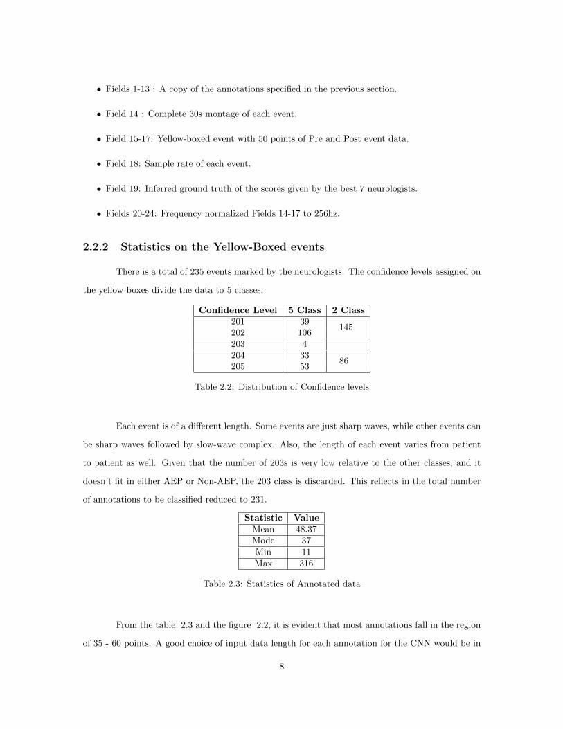
2.2.2 Statistics on the Yellow-Boxed events
There is a total of 235 events marked by the neurologists. The confidence levels assigned on
the yellow-boxes divide the data to 5 classes.
Confidence Level 5 Class 2 Class201 39
145202 106203 4204 33
86205 53
Table 2.2: Distribution of Confidence levels
Each event is of a different length. Some events are just sharp waves, while other events can
be sharp waves followed by slow-wave complex. Also, the length of each event varies from patient
to patient as well. Given that the number of 203s is very low relative to the other classes, and it
doesn’t fit in either AEP or Non-AEP, the 203 class is discarded. This reflects in the total number
of annotations to be classified reduced to 231.
Statistic ValueMean 48.37Mode 37Min 11Max 316
Table 2.3: Statistics of Annotated data
From the table 2.3 and the figure 2.2, it is evident that most annotations fall in the region
of 35 - 60 points. A good choice of input data length for each annotation for the CNN would be in
8
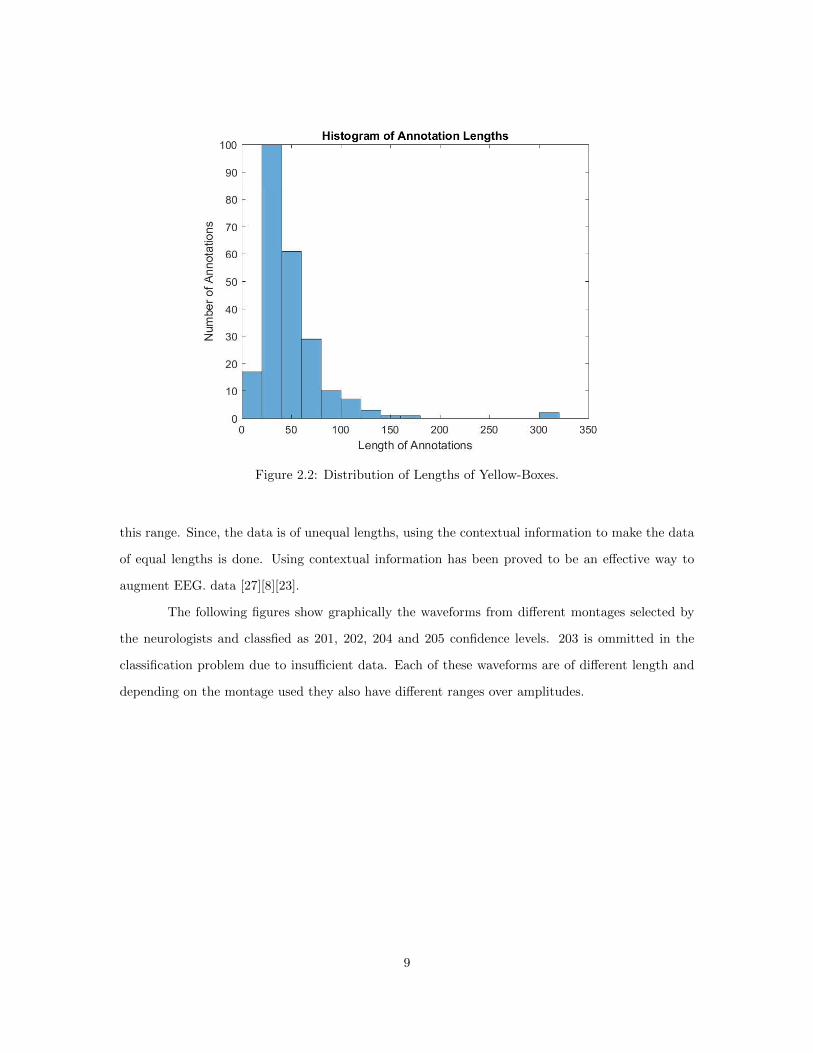
Figure 2.2: Distribution of Lengths of Yellow-Boxes.
this range. Since, the data is of unequal lengths, using the contextual information to make the data
of equal lengths is done. Using contextual information has been proved to be an effective way to
augment EEG. data [27][8][23].
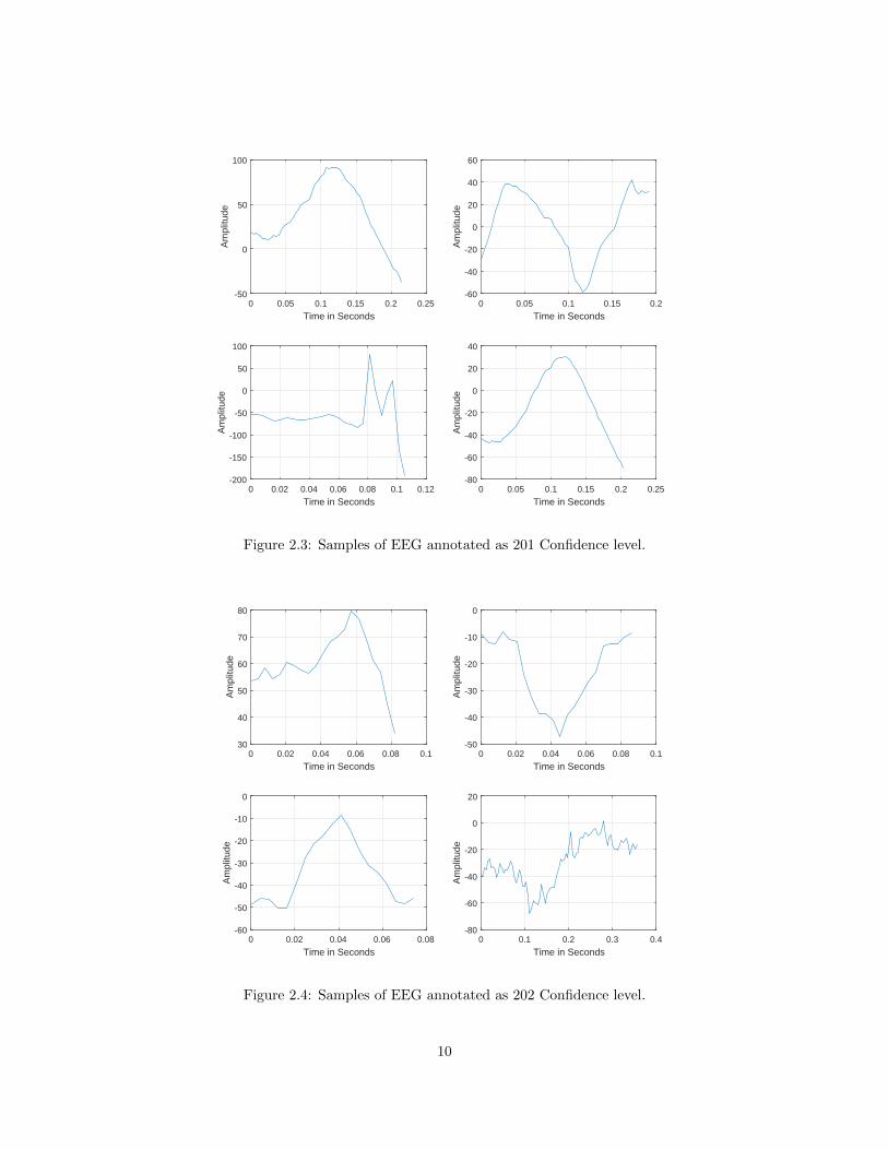
The following figures show graphically the waveforms from different montages selected by
the neurologists and classfied as 201, 202, 204 and 205 confidence levels. 203 is ommitted in the
classification problem due to insufficient data. Each of these waveforms are of different length and
depending on the montage used they also have different ranges over amplitudes.
9
0 0.05 0.1 0.15 0.2 0.25
Time in Seconds
-50
0
50
100
Am
plitu
de
0 0.05 0.1 0.15 0.2
Time in Seconds
-60
-40
-20
0
20
40
60
Am
plitu
de
0 0.02 0.04 0.06 0.08 0.1 0.12
Time in Seconds
-200
-150
-100
-50
0
50
100
Am
plitu
de
0 0.05 0.1 0.15 0.2 0.25
Time in Seconds
-80
-60
-40
-20
0
20
40
Am
plitu
de
Figure 2.3: Samples of EEG annotated as 201 Confidence level.
0 0.02 0.04 0.06 0.08 0.1
Time in Seconds
30
40
50
60
70
80
Am
plitu
de
0 0.02 0.04 0.06 0.08 0.1
Time in Seconds
-50
-40
-30
-20
-10
0
Am
plitu
de
0 0.02 0.04 0.06 0.08
Time in Seconds
-60
-50
-40
-30
-20
-10
0
Am
plitu
de
0 0.1 0.2 0.3 0.4
Time in Seconds
-80
-60
-40
-20
0
20
Am
plitu
de
Figure 2.4: Samples of EEG annotated as 202 Confidence level.
10

0 0.02 0.04 0.06 0.08 0.1
Time in Seconds
-60
-40
-20
0
20
40
Am
plitu
de
0 0.02 0.04 0.06 0.08 0.1 0.12
Time in Seconds
-70
-60
-50
-40
-30
-20
-10
Am
plitu
de
0 0.02 0.04 0.06 0.08 0.1
Time in Seconds
-100
-50
0
50
100
Am
plitu
de
0 0.05 0.1 0.15 0.2 0.25
Time in Seconds
-150
-100
-50
0
50
100
Am
plitu
de
Figure 2.5: Samples of EEG annotated as 204 Confidence level.
0 0.02 0.04 0.06 0.08 0.1
Time in Seconds
-20
0
20
40
60
Am
plitu
de
0 0.02 0.04 0.06 0.08 0.1
Time in Seconds
-40
-30
-20
-10
0
Am
plitu
de
0 0.05 0.1 0.15
Time in Seconds
-20
0
20
40
60
80
Am
plitu
de
0 0.02 0.04 0.06 0.08
Time in Seconds
-50
0
50
100
150
200
Am
plitu
de
Figure 2.6: Samples of EEG annotated as 205 Confidence level.
11

Chapter 3
Convolutional Neural Network
Basics
Deep Learning refers to a branch of machine learning that is based on learning levels of
representations. Convolutional neural networks are one kind of deep neural networks which are
powerful models that yield hierarchies of features, helps in understanding data such as images, time-
series data, text . . . etc. ConvNets/CNNs have been employed in character recognition tasks as early
as the nineties [4][17], ConvNets rose to widespread application when a deep CNN was used to beat
state-of-the-art in the ImageNet image classification challenge in 2012 [16]. This chapter intends to
give the background necessary in convolutional neural networks used in this research undertaking.
The explanations presented lean heavily on the following resources [6] [33] [18] [28] [36] [19] [26].
Most literature available on CNNs is for the 2-D counterpart. This thesis explains the architecture
in 1-D by condensing the equations from 2-D structures explained in the above references to 1-D.
3.1 Fully Connected Networks
A basic feed-forward neural network is a fully connected neural network in which each neuron
is connected to every neuron in the previous layer. There is a directionality in these connections,
where these linear combinations are input to a, usually non-linear, activation function to form the
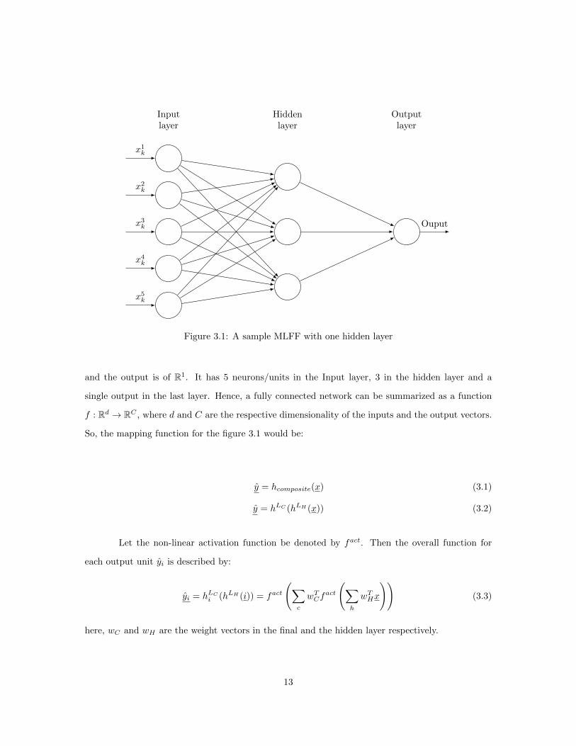
input of the next layer or the output if it’s the last layer. In the figure 3.1, the input is of R5
12
Inputlayer
Hiddenlayer
Outputlayer
x1k
x2k
x3k
x4k
x5k
Ouput
Figure 3.1: A sample MLFF with one hidden layer
and the output is of R1. It has 5 neurons/units in the Input layer, 3 in the hidden layer and a
single output in the last layer. Hence, a fully connected network can be summarized as a function
f : Rd → RC , where d and C are the respective dimensionality of the inputs and the output vectors.
So, the mapping function for the figure 3.1 would be:
y = hcomposite(x) (3.1)
y = hLC (hLH (x)) (3.2)
Let the non-linear activation function be denoted by fact. Then the overall function for
each output unit yi is described by:
yi = hLCi (hLH (i)) = fact
(∑c
wTCf
act
(∑h
wTHx
))(3.3)
here, wC and wH are the weight vectors in the final and the hidden layer respectively.
13
3.2 Activation Functions
Activation functions are a major decision point while designing neural network architectures.
They determine how the inputs from a previous layer are transformed and input to the next layer.
While, activation functions can be linear, linear activation implies the unit is a linear combination
of the previous layer which, sometimes, inhibits the network to learn depending the complexity of
the problem. Also, there is the problem of the activation to be non-saturating leading to large error
corrections during back-propogation with small changes to the input, which is undesirable. Hence,
non-linear activations are usually preferred.
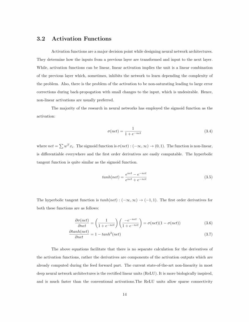
The majority of the research in neural networks has employed the sigmoid function as the
activation:
σ(net) =1
1 + e−net(3.4)
where net =∑wTxi. The sigmoid function is σ(net) : (−∞,∞)→ (0, 1). The function is non-linear,
is differentiable everywhere and the first order derivatives are easily computable. The hyperbolic
tangent function is quite similar as the sigmoid function.
tanh(net) =enet − e−net
enet + e−net(3.5)
The hyperbolic tangent function is tanh(net) : (−∞,∞) → (−1, 1). The first order derivatives for
both these functions are as follows:
∂σ(net)
∂net=
(1
1 + e−net
)(−e−net
1 + e−net
)= σ(net)(1− σ(net)) (3.6)
∂tanh(net)
∂net= 1− tanh2(net) (3.7)
The above equations facilitate that there is no separate calculation for the derivatives of
the activation functions, rather the derivatives are components of the activation outputs which are
already computed during the feed forward part. The current state-of-the-art non-linearity in most
deep neural network architectures is the rectified linear units (ReLU). It is more biologically inspired,
and is much faster than the conventional activations.The ReLU units allow sparse connectivity
14
-3 -2 -1 0 1 2 3-3
-2
-1
0
1
2
3
SigmoidTanhReLU
Figure 3.2: Behaviour of Sigmoid, Hyperbolic Tangent and Rectilinear activation functions withinput [-3,3]
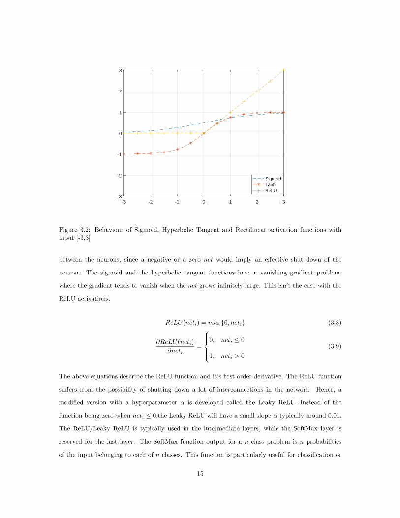
between the neurons, since a negative or a zero net would imply an effective shut down of the
neuron. The sigmoid and the hyperbolic tangent functions have a vanishing gradient problem,
where the gradient tends to vanish when the net grows infinitely large. This isn’t the case with the
ReLU activations.
ReLU(neti) = max{0, neti} (3.8)
∂ReLU(neti)
∂neti=
0, neti ≤ 0
1, neti > 0
(3.9)
The above equations describe the ReLU function and it’s first order derivative. The ReLU function
suffers from the possibility of shutting down a lot of interconnections in the network. Hence, a
modified version with a hyperparameter α is developed called the Leaky ReLU. Instead of the
function being zero when neti ≤ 0,the Leaky ReLU will have a small slope α typically around 0.01.
The ReLU/Leaky ReLU is typically used in the intermediate layers, while the SoftMax layer is
reserved for the last layer. The SoftMax function output for a n class problem is n probabilities
of the input belonging to each of n classes. This function is particularly useful for classification or
15

prediction layers:
P (Class(i) = j|net) =enetj∑nk=1 e
netk. (3.10)
3.2.1 One-hot encoding
A categorical variable describes the class of an input. One-hot encoding is typically used
in CNNs. It transforms the categorical variable into a format which works better with classification
and regression algorithms. For example, for a C class problem and a categorical variable or the
ground truth y, one-hot encoding transforms it to a C dimensional vector y. Both y and output
from SoftMax y are probability mass functions. The one-hot encoding used in this thesis is shown
below:
Category Class Encoding201 Non-
AEP1 0
202204
AEP 0 1205
Table 3.1: One-hot encoding of AEP and Non-AEP
Category Class Encoding201 Definitely not AEP 1 0 0 0202 Unlikely to be AEP 0 1 0 0204 Likely to be AEP 0 0 1 0205 Definitely an AEP 0 0 0 1
Table 3.2: One-hot encoding for 4 Confidence levels
3.3 Gradient Descent Optimization
A neural network for classification or regression learns through minimizing it’s loss function
in the prediction layer. There are many different types of loss functions. For example, where L(w)
is the total loss, a simple loss function could be
L(w) =∑ 1
2||y − y||2 (3.11)
16
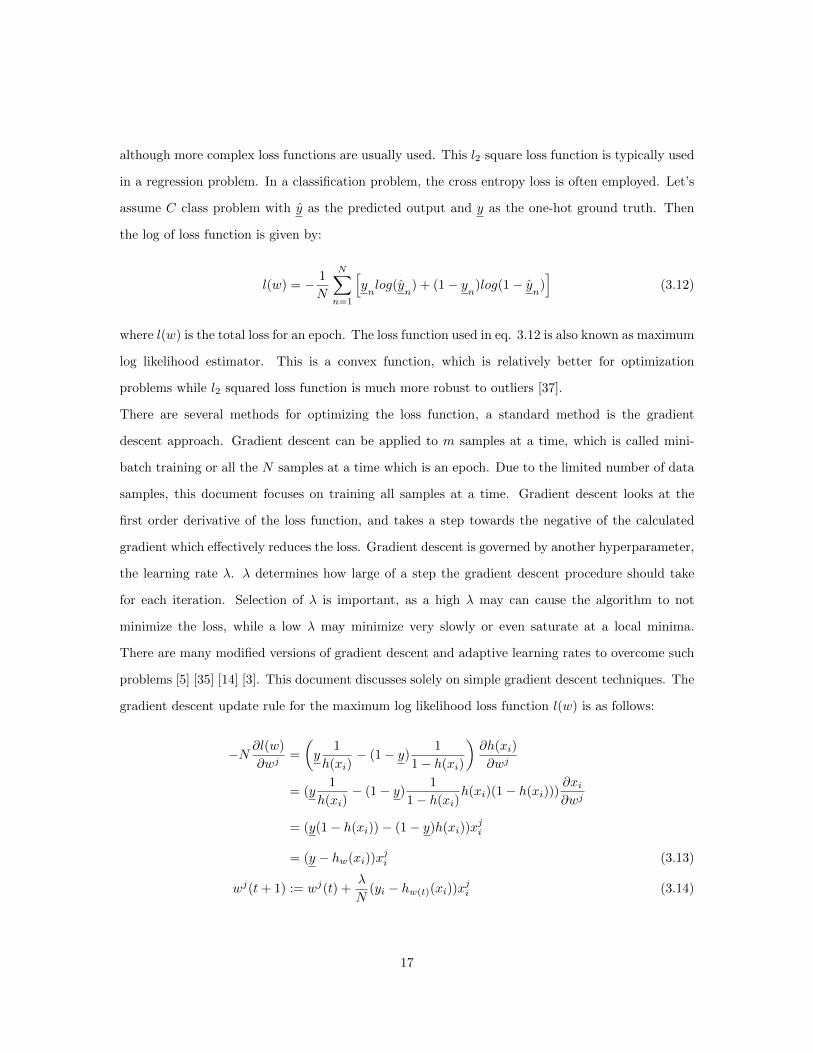
although more complex loss functions are usually used. This l2 square loss function is typically used
in a regression problem. In a classification problem, the cross entropy loss is often employed. Let’s
assume C class problem with y as the predicted output and y as the one-hot ground truth. Then
the log of loss function is given by:
l(w) = − 1
N
N∑n=1
[ynlog(y
n) + (1− y
n)log(1− y
n)]
(3.12)
where l(w) is the total loss for an epoch. The loss function used in eq. 3.12 is also known as maximum
log likelihood estimator. This is a convex function, which is relatively better for optimization
problems while l2 squared loss function is much more robust to outliers [37].
There are several methods for optimizing the loss function, a standard method is the gradient
descent approach. Gradient descent can be applied to m samples at a time, which is called mini-
batch training or all the N samples at a time which is an epoch. Due to the limited number of data
samples, this document focuses on training all samples at a time. Gradient descent looks at the
first order derivative of the loss function, and takes a step towards the negative of the calculated
gradient which effectively reduces the loss. Gradient descent is governed by another hyperparameter,
the learning rate λ. λ determines how large of a step the gradient descent procedure should take
for each iteration. Selection of λ is important, as a high λ may can cause the algorithm to not
minimize the loss, while a low λ may minimize very slowly or even saturate at a local minima.
There are many modified versions of gradient descent and adaptive learning rates to overcome such
problems [5] [35] [14] [3]. This document discusses solely on simple gradient descent techniques. The
gradient descent update rule for the maximum log likelihood loss function l(w) is as follows:
−N ∂l(w)
∂wj=
(y
1
h(xi)− (1− y)
1
1− h(xi)
)∂h(xi)
∂wj
= (y1
h(xi)− (1− y)
1
1− h(xi)h(xi)(1− h(xi)))
∂xi∂wj
= (y(1− h(xi))− (1− y)h(xi))xji
= (y − hw(xi))xji (3.13)
wj(t+ 1) := wj(t) +λ
N(yi − hw(t)(xi))x
ji (3.14)
17

where y = h(x) and x is the input from the previous layer, the weights for (t+ 1)th iteration would
be as described in eq. 3.14. Let δlj be the output deviation of ylj , i.e. unit j in layer l. Then from the
generalized delta rule, the weight adjustment strategy for every subsequent previous layer is defined
as follows:
δlj = (yj − yj)f ′j(netlj) (3.15)
δl−1j = δljwl−1T f ′j(net
l−1j ) (3.16)
This process is repeated till l − 1 = 1 i.e. till it reaches the input layer.
Instead of using a constant learning rate, a decay parameter is introduced. Optimization
problems usually converge faster in the early iterations and saturate. Decay in the learning rate as
a function of iteration helps in reducing the learning rate to fine tune the loss optimization. The
learning rate used is as follows:
λ = λmin + (λmax − λmin)e−iα (3.17)
here i is the iteration number, λmin and λmax are the minimum and maximum constraints on the
learning rate and the parameter α regulates the rate of decay of learning rate from λmax to λmin
3.4 Convolution Layer Forward Pass
The convolution layer has an input and kernels associated with it. Kernels/Filters is the
commonly used terms for groups of weights in convolution layers. The Convolution layer shares
weights, in the sense that the weights are slid across the input and convolved to give a feature map
for that particular weight vector. The convolutions can be strided, where stride is the increment in
the number of positions where the next convolution takes place. Zero padding can be done for the
input of the convolution layer. For an input size of i, stride s, and padding p, the size of the feature
map thus generated is:
o =
⌊(i+ 2p− k)
s
⌋+ 1 (3.18)
18

The input size is chosen such that it conforms to the stride division in each convolution layers. This
thesis uses half padding with unit stride, where the input size equals output size after convolution
for CNN1 architecture. The k chosen is always odd, hence from the equation 3.18, o = i can be
derived for unit stride. There are multiple weight vectors/filters in each convolution layer giving rise
to corresponding feature maps. Each of these feature maps are Batch-Normalized [11]. For large
training sets, the training is done in batches. During back-propagation, the layers continually adapt
to reduce the output error, this change in the distributions of internal nodes of a deep network is
referred to as Internal Covariance Shift. This phenomenon usually results in saturation and vanishing
gradient problems. Hence, all the convolution output feature maps are normalized as follows:
xk =xk − E[xk]√V ar[xk] + ε
(3.19)
yk = γxk + β (3.20)
Here, E[ ] is the expectation operation, V ar[ ] is the variance operation, ε is a small positive constant.
This ensures the feature maps transform to unit Gaussian activations. The output is then shifted
by learned parameters β and scaled by γ. These parameters are learned through back-propagation,
which determine the best characteristics of shift and scale for the data to go through activation.
γ = 1.0 and β = 0 are the typical initializations of these parameters.
Figure 3.3: Block Diagram for a typical Convolution Layer
Normalizing helps in faster training and regularizes the network. Using normalization,
learning rate can be increased with no-ill side effects. The normalized feature maps are activated
with a suitable activation function, typically the ReLU. A dropout mechanism is introduced in the
19
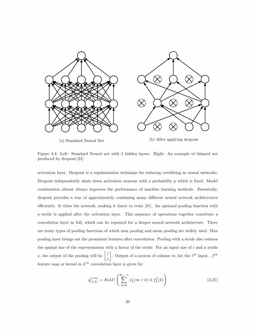
(a) Standard Neural Net (b) After applying dropout
Figure 3.4: Left: Standard Neural net with 2 hidden layers. Right: An example of thinned netproduced by dropout.[31]
activation layer. Dropout is a regularization technique for reducing overfitting in neural networks.
Dropout independently shuts down activation neurons with a probability p which is fixed. Model
combination almost always improves the performance of machine learning methods. Essentially,
dropout provides a way of approximately combining many different neural network architectures
efficiently. It thins the network, making it faster to train [31]. An optional pooling function with
a stride is applied after the activation layer. This sequence of operations together constitute a
convolution layer in full, which can be repeated for a deeper neural network architecture. There
are many types of pooling functions of which max pooling and mean pooling are widely used. Max
pooling layer brings out the prominent features after convolution. Pooling with a stride also reduces
the spatial size of the representation with a factor of the stride. For an input size of i and a stride
s, the output of the pooling will be
⌊i
s
⌋. Output of a neuron of column m, for the ith input , f th
feature map or kernel in Lth convolution layer is given by:
y(i,m)(f,L) = ReLU
(KL−1∑k=0
xiL(m+ k) ~ ffL(k)
)(3.21)
20
where KL is the total number of kernels in the Lth layer. The further max pooling operation follows
accordingly for input x and output y:
y(i,m)(f,L) = max(xil(m− (s− 1)), xiL(m(s− 2)), . . . , xiL(m)) (3.22)
where, the pooling operation usually starts at the stride index s and increments to m+s for the next
max-pooling operation. At the end of the convolution layers, the number of feature maps generated
will be FF = K1×K2 · · ·×KL. The last convolution layer is typically connected to a fully connected
network. Therefore, for a training set H ∈ RN×d, the input to the fully connected network is of
RN×FF×o. Each feature map is now stacked row-wise to form an input of RN×(FF×o). The fully
connected layer can consist of many hidden layers and then a final SoftMax output layer. This
functions as described in the previous sections. The output error is calculated at the output layer
and is back-propagated as per the equations 3.15 and 3.16 till the beginning of the last convolution
layer.
3.5 Convolution Layer Back-Propagation
The calculated δlj ∈ RN×(FF×o). This is re-stacked to RN×FF×o, to match the dimension-
ality of the feature maps at the last convolution layer. As there is no gradient for the non-maximum
parts that do not come through the max pooling layer, the δlj ∈ RN×FF×(KL×o) with
δlp =
0 if p = nonmax unit.
otherwise, gradient from re-stacked δ (δlj)
(3.23)
The δl−1p for the previous convolution layer is calculated by convolving δlp with filters of that layer
fKl−1
L−1 .
δl−1p = δlp ~ fKl
l (3.24)
21

The kernel adjustment strategy is as follows:
ffL = ffL −λ
KL
KL∑f=1
δfL ~ xiL (3.25)
The convolution follows the dimensionality specified in the eq.3.18.
3.6 Convolution Neural Network Architectures
3.6.1 Architecture 1- CNN1
Figure 3.5 represents the CNN1 architecture used in this thesis. The input size of each
input vector is fixed at 40. In the first convolution layer, 6 filters of each size 7 are initialized. Since,
the pre-epileptic spike is of 20-70ms duration, an appropriate filter size length should be in this
range to capture the characteristics that differentiate each segment from the other. Hence, 7 in the
first convolution layer and 5 in the next layer are chosen. The filters are convolved with unit stride
with the input to give 6 feature maps each from the corresponding filter. These feature maps are
activated with the ReLU activation without dropout and input to max-pooling layer with stride =
2. This reduces the dimensionality of the feature maps by a factor of 2. Further, output feature
maps are convolved with another set of 6 filters of size 5, to give 6×6 feature maps. The sequence of
operations is repeated to give 36 feature maps of length 10 each. The convolution network furthers
into a fully connected network. Fully connected networks are densely connected while Convolution
Layers have sparse connectivity, using dropout in the convolution layers greatly effects the outputs,
which is undesirable. Dropout is used in the fully connected layers with probability of keeping a
neuron P (keep) = 0.75. There are 2 hidden layers in the fully connected network. The first network
has a 360× 200 weight network to give an output of length 200. The last fully connected layer has
a 200× C weight network with the activation as the SoftMax activation, where C is the number of
classes the network classifies to. The SoftMax layer calculates the probability of each input belonging
to any of the classes. The class with the highest probability is chosen as the classification output.
22

Figure 3.5: Convolution Neural Network Architecture 1 - CNN1
3.6.2 Architecture 2 - CNN2
Figure 3.6 represents the CNN2 architecture used in this thesis. The input size of each input
vector is fixed at 40. In the first convolution layer, 6 filters of each size 7 are initialized. The filter
sizes in each subsequent convolution layer are 7, 5, and 3. The filters are convolved with unit stride
with the input to give 6 feature maps each from the corresponding filter. The feature maps are
normalized and are activated with the ReLU activation without dropout. This does not reduce the
dimensionality of the feature maps. Further, output feature maps are convolved with stride = 2 with
another set of 6 filters of size 5, to give 6× 6 feature maps. The sequence of operations is repeated
to give 36 feature maps of length 20 each. The sequence of operations is repeated to give 144 feature
23

maps of length 10 each. The convolution network furthers into a fully connected network. Dropout
is used in the fully connected layers with probability of keeping a neuron P (keep) = 0.75. There are
2 hidden layers in the fully connected network. The first network has a 1440× 400 weight network
to give an output of length 200. The last fully connected layer has a 400× C weight network with
the activation as the SoftMax activation. The SoftMax layer calculates the probability of each input
belonging to any of the classes. The class with the highest probability is chosen as the classification
output.
Figure 3.6: Convolution Neural Network Architecture 2 - CNN2
24

Chapter 4
Detection of Yellow-Boxes
To detect the Yellow-Boxes in the EEG, first the convolution neural network architectures
are trained to discriminate between Yellow-Boxes and Non-Yellow Boxes. The EEG data of over
200 patients together contribute to 235 Yellow-Boxes. All other EEG segments are not annotated
by the neurologists and hence, can be considered as Non-Yellow Boxed segments. For the CNN1,
the input data is scaled to fit in the range (0, 1). For CNN2, normalization is used. Different EEG
segments occur in different amplitude regions and ranges. Hence, standardizing these input vectors
is needed to weight each input vector’s characteristic equally.
4.1 Approach
Detection of yellow-boxes can be approached in two ways:
• Using a cascade network architecture to bifurcate the EEG data into yellow-boxes or otherwise
and then the classification of Yellow-Boxes.
• Using the non-annotated data as a class extension to the regular 2 or 4 class Yellow-Box
classification problem to make it a 3 or 5 class problem where one class represents non-yellow-
boxed data while others include classified yellow-boxed data.
DBY2, DYB3 and DYB5 stand for Detection of Yellow-Boxes treated as 2 class problem, treated as
a class extion to 2 class and 4 class Yellow-Box Classification respectively. The block diagram for
these approaches is shown in the following figures:
25

Figure 4.1: Block Diagram for Detection of Yellow-Boxes and classification of Detected Yellow-Boxes
Figure 4.2: Block Diagram for Detection Network as Class Extension (3 Class) DYB3
Figure 4.3: Block Diagram for Detection Network as Class Extension (5 Class) DYB5
26

FN TN
TP FPC1
C2
C1 C2
Pre
dic
ted
Cla
ss
True Class
Figure 4.4: Confusion Matrix for a 2 Class Problem
4.2 Performance Metrics
A confusion matrix best represents the outputs of predictive analysis algorithms. It is
typically a matrix of C × C, a case where C = 2 is shown here.
• A True Positive (TP) is when the classifier output and the ground truth are both positive.
• A True Negative (TN) is when the classifier output and the ground truth are both negative.
• A False Positive (FP) is when the classifier output is positive while the ground truth is negative.
• A False Negative (FN) is when the classifier output is negative while the ground truth is
positive.
The performance of a classifier is evaluated using certain performance parameters shown below:
• Sensitivity: It is called the True Positive Rate, the proportion of positives correctly identified
from total number of positives.
Sensitivity =TruePositives
Total No. of Positives(4.1)
27

• Specificity: It is called the True Negative Rate, the proportion of negatives correctly identified
from total number of negatives.
Specificity =TrueNegatives
Total No. of Negatives(4.2)
• Selectivity/Precision: It is called the Positive Predictive Value, the proportion of positives
correctly identified.
Selectivity =TruePositives
PositiveOutputs(4.3)
4.3 Data - DYB2 Problem
The Non-Yellow Box data is selected randomly from all the 200 patient records which are
not annotated as Yellow-Box. As the Yellow-Boxes are 235 in number, equal number of Non-Yellow
Box data is generated. This data is used with both CNN1 and CNN2 architectures for detection of
Yellow-Boxes.
4.3.1 Training Hyperparameters
• All weights are initialized as random numbers between [-ε, ε], where ε = 0.01.
• The learning rate λ has λmax = 0.003 and λmin = 0.0001 with a decay α = 100.
• Input vector size is 40.
• Number of iterations is 500 for CNN1 and 200 for CNN2.
• CNN1 Filter size is 7 in the first Convolution layer, and a size of 5 on the second Convolution
layer.
• CNN2 Filter size is 7 in the first Convolution layer, a size of 5 on the second Convolution layer,
and a size of 3 on the third Convolution layer.
These parameters give good convergence in the Loss vs Iteration plots i.e. the loss function doesn’t
change much after the number of iterations specified for each architecture.
28
4.3.2 Cross Validation
Cross-Validation is a technique to evaluate classification models by partitioning the original
dataset into training and testing sets. In K-fold cross validation, the dataset is split into K-1:1 ratio
of training and testing respectively. This technique assesses how well the model will generalize to
an independent dataset. K-fold cross validation is performed with K from 4 to 10.
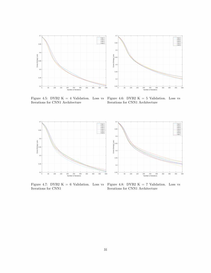
4.3.3 DYB2 Results - CNN1
Both the CNN architectures are used to detect the Yellow-Boxes. This section includes the
data split of Non-Yellow Boxes and Yellow-Boxes, plots of Loss vs Iterations for each fold of K-fold
validation, performance metrics of the CNN1 architecture, average performance over all the folds
for each K in 4 to 10.
29

No. of Folds Fold No. No. of Non-YB No. of YB Ratio Non-YB/YB Total
4
1 85 60 1.41 1452 67 69 0.97 1363 66 79 0.83 1454 72 73 0.98 145
5
1 59 57 1.03 1162 66 44 1.50 1103 57 59 0.96 1164 51 65 0.78 1165 57 59 0.96 116
6
1 46 51 0.90 972 53 36 1.47 893 42 55 0.76 974 51 46 1.10 975 50 47 1.06 976 48 49 0.97 97
7
1 42 41 1.02 832 40 46 0.86 863 33 50 0.66 834 41 42 0.97 835 38 45 0.84 836 50 33 1.52 837 47 36 1.30 83
8
1 35 38 0.92 732 41 40 1.02 813 35 38 0.92 734 36 37 0.97 735 44 29 1.51 736 37 36 1.02 737 30 43 0.69 738 34 39 0.87 73
9
1 33 32 1.03 652 30 35 0.85 653 39 26 1.50 654 32 33 0.96 655 37 28 1.32 656 26 39 0.66 657 30 35 0.85 658 37 28 1.32 659 27 38 0.71 65
10
1 24 34 0.70 582 30 25 1.20 553 32 26 1.23 584 23 35 0.65 585 31 27 1.14 586 25 33 0.75 587 30 28 1.07 588 36 22 1.63 589 31 27 1.14 5810 28 30 0.93 58
Table 4.1: Distribution of Data for DYB2 of Yellow-Boxes
30
0 50 100 150 200 250 300 350 400 450 500
Number of Iterations
0.4
0.45
0.5
0.55
0.6
0.65
0.7C
ross
Ent
ropy
Los
sFold 1Fold 2Fold 3Fold 4
Figure 4.5: DYB2 K = 4 Validation. Loss vsIterations for CNN1 Architecture
0 50 100 150 200 250 300 350 400 450 500
Number of Iterations
0.35
0.4
0.45
0.5
0.55
0.6
0.65
0.7
Cro
ss E
ntro
py L
oss
Fold 1Fold 2Fold 3Fold 4Fold 5
Figure 4.6: DYB2 K = 5 Validation. Loss vsIterations for CNN1 Architecture
0 50 100 150 200 250 300 350 400 450 500
Number of Iterations
0.4
0.45
0.5
0.55
0.6
0.65
0.7
Cro
ss E
ntro
py L
oss
Fold 1Fold 2Fold 3Fold 4Fold 5Fold 6
Figure 4.7: DYB2 K = 6 Validation. Loss vsIterations for CNN1
0 50 100 150 200 250 300 350 400 450 500
Number of Iterations
0.35
0.4
0.45
0.5
0.55
0.6
0.65
0.7
Cro
ss E
ntro
py L
oss
Fold 1Fold 2Fold 3Fold 4Fold 5Fold 6Fold 7
Figure 4.8: DYB2 K = 7 Validation. Loss vsIterations for CNN1 Architecture
31
0 50 100 150 200 250 300 350 400 450 500
Number of Iterations
0.35
0.4
0.45
0.5
0.55
0.6
0.65
0.7C
ross
Ent
ropy
Los
sFold 1Fold 2Fold 3Fold 4Fold 5Fold 6Fold 7Fold 8
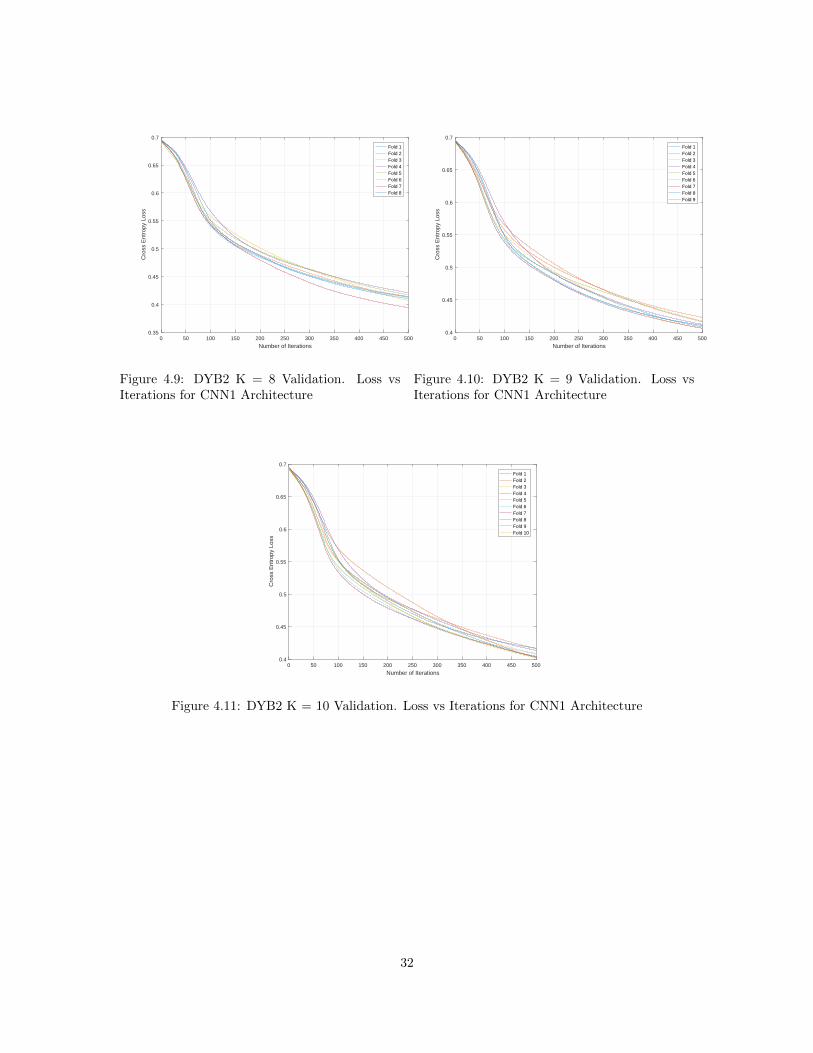
Figure 4.9: DYB2 K = 8 Validation. Loss vsIterations for CNN1 Architecture
0 50 100 150 200 250 300 350 400 450 500
Number of Iterations
0.4
0.45
0.5
0.55
0.6
0.65
0.7
Cro
ss E
ntro
py L
oss
Fold 1Fold 2Fold 3Fold 4Fold 5Fold 6Fold 7Fold 8Fold 9
Figure 4.10: DYB2 K = 9 Validation. Loss vsIterations for CNN1 Architecture
0 50 100 150 200 250 300 350 400 450 500
Number of Iterations
0.4
0.45
0.5
0.55
0.6
0.65
0.7
Cro
ss E
ntro
py L
oss
Fold 1Fold 2Fold 3Fold 4Fold 5Fold 6Fold 7Fold 8Fold 9Fold 10
Figure 4.11: DYB2 K = 10 Validation. Loss vs Iterations for CNN1 Architecture
32

No. of Folds Fold No. Specificity Sensitivity Selectivity Accuracy
4
1 0.91304 0.71053 0.9 0.80692 0.88889 0.76829 0.91304 0.816183 0.6875 0.7284 0.74684 0.710344 0.77333 0.8 0.76712 0.78621
5
1 0.84615 0.76563 0.85965 0.801722 0.86207 0.69231 0.81818 0.781823 0.75 0.82692 0.72881 0.784484 0.73913 0.75714 0.81538 0.755 0.82 0.75758 0.84746 0.78448
6
1 0.87805 0.82143 0.90196 0.845362 0.87805 0.64583 0.86111 0.752813 0.775 0.80702 0.83636 0.793814 0.82609 0.7451 0.82609 0.783515 0.88636 0.79245 0.89362 0.835056 0.77273 0.73585 0.79592 0.75258
7
1 0.77778 0.81579 0.7561 0.795182 0.7619 0.81818 0.78261 0.79073 0.6875 0.78431 0.8 0.746994 0.70732 0.71429 0.71429 0.710845 0.88462 0.73684 0.93333 0.783136 0.82609 0.67568 0.75758 0.759047 0.86486 0.67391 0.86111 0.75904
8
1 0.66667 0.73529 0.65789 0.698632 0.65789 0.62791 0.675 0.641983 0.85714 0.86842 0.86842 0.863014 0.78378 0.80556 0.78378 0.794525 0.80435 0.74074 0.68966 0.780826 0.78378 0.77778 0.77778 0.780827 0.83333 0.79592 0.90698 0.808228 0.8125 0.80488 0.84615 0.80822
9
1 0.80645 0.76471 0.8125 0.784622 0.8 0.82857 0.82857 0.815383 0.83333 0.68966 0.76923 0.769234 0.82353 0.87097 0.81818 0.846155 0.84211 0.81481 0.78571 0.830776 0.7037 0.81579 0.79487 0.769237 0.78571 0.78378 0.82857 0.784628 0.8 0.62857 0.78571 0.707699 0.75 0.78049 0.84211 0.76923
10
1 0.80769 0.90625 0.85294 0.862072 0.82143 0.74074 0.8 0.781823 0.74194 0.66667 0.69231 0.70694 0.75862 0.96552 0.8 0.862075 0.81481 0.70968 0.81481 0.758626 0.69231 0.78125 0.75758 0.741387 0.84615 0.75 0.85714 0.79318 0.96296 0.67742 0.95455 0.810349 0.93103 0.86207 0.92593 0.8965510 0.70968 0.77778 0.7 0.74138
Table 4.2: Performance Metrics for DYB2 of Yellow-Boxes for CNN1 Architecture
33
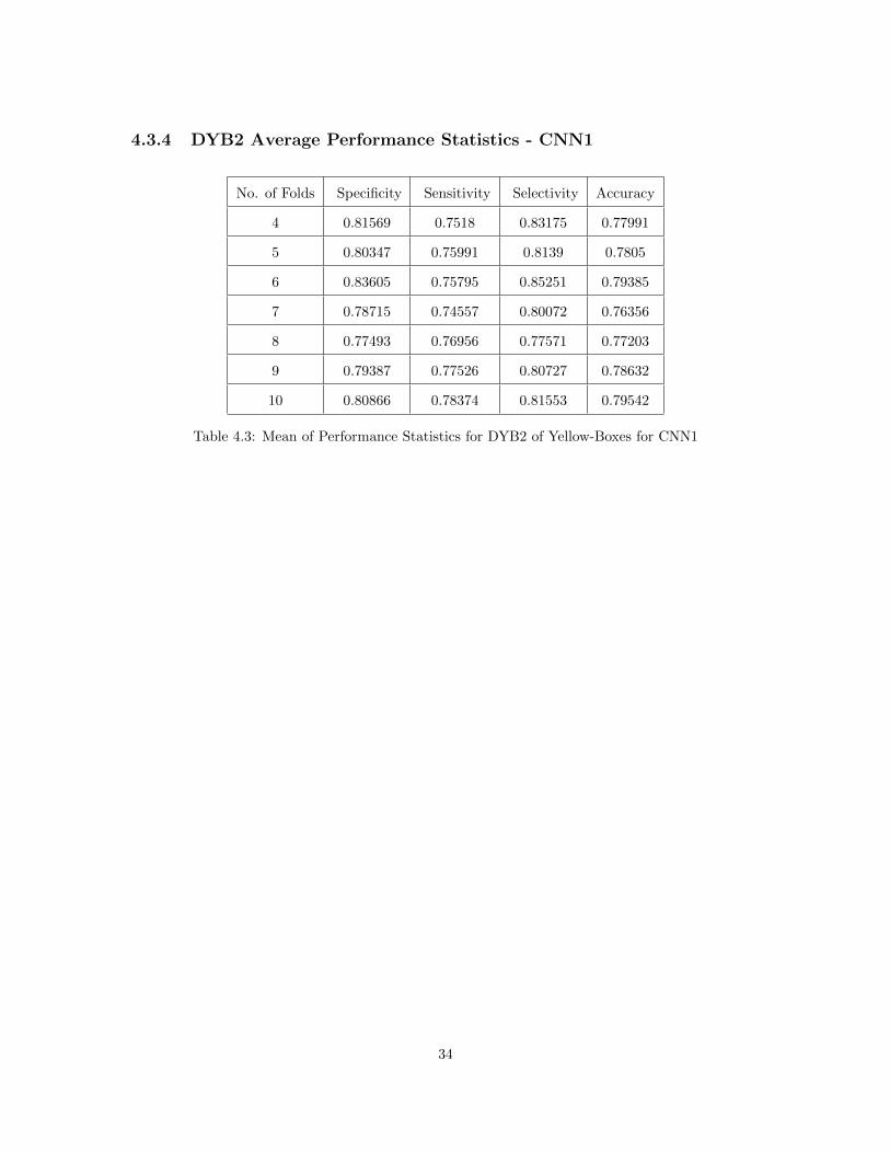
4.3.4 DYB2 Average Performance Statistics - CNN1
No. of Folds Specificity Sensitivity Selectivity Accuracy
4 0.81569 0.7518 0.83175 0.77991
5 0.80347 0.75991 0.8139 0.7805
6 0.83605 0.75795 0.85251 0.79385
7 0.78715 0.74557 0.80072 0.76356
8 0.77493 0.76956 0.77571 0.77203
9 0.79387 0.77526 0.80727 0.78632
10 0.80866 0.78374 0.81553 0.79542
Table 4.3: Mean of Performance Statistics for DYB2 of Yellow-Boxes for CNN1
34
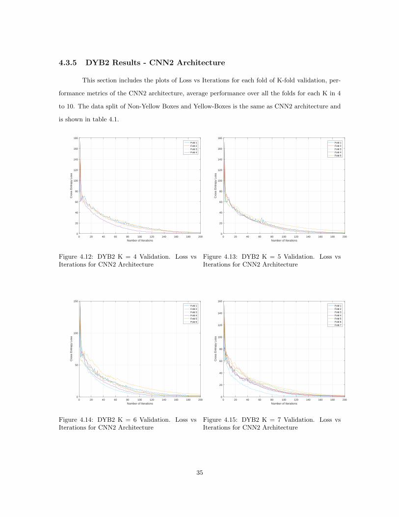
4.3.5 DYB2 Results - CNN2 Architecture
This section includes the plots of Loss vs Iterations for each fold of K-fold validation, per-
formance metrics of the CNN2 architecture, average performance over all the folds for each K in 4
to 10. The data split of Non-Yellow Boxes and Yellow-Boxes is the same as CNN2 architecture and
is shown in table 4.1.
0 20 40 60 80 100 120 140 160 180 200
Number of Iterations
0
20
40
60
80
100
120
140
160
180
Cro
ss E
ntro
py L
oss
Fold 1Fold 2Fold 3Fold 4
Figure 4.12: DYB2 K = 4 Validation. Loss vsIterations for CNN2 Architecture
0 20 40 60 80 100 120 140 160 180 200
Number of Iterations
0
20
40
60
80
100
120
140
160
180
Cro
ss E
ntro
py L
oss
Fold 1Fold 2Fold 3Fold 4Fold 5
Figure 4.13: DYB2 K = 5 Validation. Loss vsIterations for CNN2 Architecture
0 20 40 60 80 100 120 140 160 180 200
Number of Iterations
0
50
100
150
Cro
ss E
ntro
py L
oss
Fold 1Fold 2Fold 3Fold 4Fold 5Fold 6
Figure 4.14: DYB2 K = 6 Validation. Loss vsIterations for CNN2 Architecture
0 20 40 60 80 100 120 140 160 180 200
Number of Iterations
0
20
40
60
80
100
120
140
160
Cro
ss E
ntro
py L
oss
Fold 1Fold 2Fold 3Fold 4Fold 5Fold 6Fold 7
Figure 4.15: DYB2 K = 7 Validation. Loss vsIterations for CNN2 Architecture
35
0 20 40 60 80 100 120 140 160 180 200
Number of Iterations
0
20
40
60
80
100
120
140
160
180C
ross
Ent
ropy
Los
sFold 1Fold 2Fold 3Fold 4Fold 5Fold 6Fold 7Fold 8
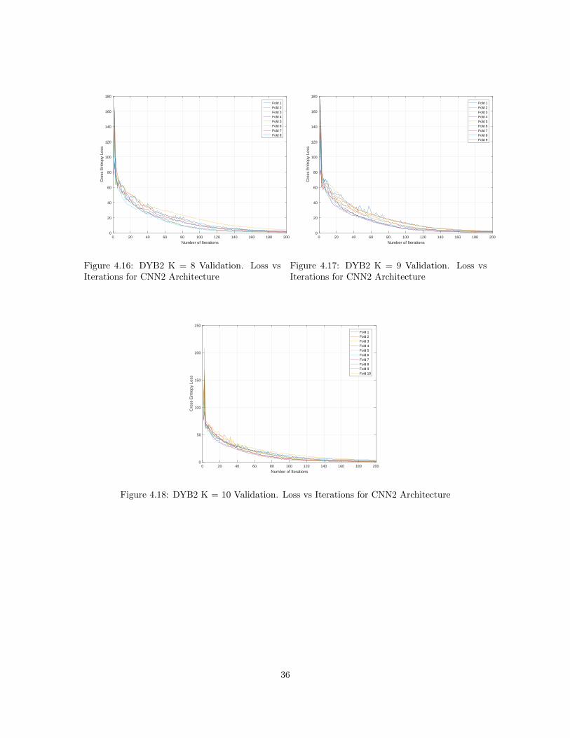
Figure 4.16: DYB2 K = 8 Validation. Loss vsIterations for CNN2 Architecture
0 20 40 60 80 100 120 140 160 180 200
Number of Iterations
0
20
40
60
80
100
120
140
160
180
Cro
ss E
ntro
py L
oss
Fold 1Fold 2Fold 3Fold 4Fold 5Fold 6Fold 7Fold 8Fold 9
Figure 4.17: DYB2 K = 9 Validation. Loss vsIterations for CNN2 Architecture
0 20 40 60 80 100 120 140 160 180 200
Number of Iterations
0
50
100
150
200
250
Cro
ss E
ntro
py L
oss
Fold 1Fold 2Fold 3Fold 4Fold 5Fold 6Fold 7Fold 8Fold 9Fold 10
Figure 4.18: DYB2 K = 10 Validation. Loss vs Iterations for CNN2 Architecture
36

No. of Folds Fold No. Specificity Sensitivity Selectivity Accuracy
4
1 0.87013 0.86765 0.85507 0.868972 0.82759 0.73256 0.86301 0.770833 0.84286 0.82667 0.84932 0.834484 0.86486 0.90141 0.86486 0.88276
5
1 0.875 0.84615 0.84615 0.862072 0.87302 0.80392 0.83673 0.842113 0.78333 0.85714 0.78689 0.818974 0.90385 0.84375 0.91525 0.870695 0.76667 0.94643 0.79104 0.85345
6
1 0.89796 0.91667 0.89796 0.907222 0.88372 0.89362 0.89362 0.888893 0.95652 0.84314 0.95556 0.896914 0.87234 0.8 0.86957 0.835055 0.74074 0.86047 0.72549 0.793816 0.84906 0.88636 0.82979 0.86598
7
1 0.90909 0.79487 0.88571 0.855422 0.87097 0.82609 0.90476 0.844163 0.86047 0.9 0.85714 0.879524 0.90244 0.85714 0.9 0.879525 0.90244 0.95238 0.90909 0.927716 0.83673 0.85294 0.78378 0.843377 0.77273 0.89744 0.77778 0.83133
8
1 0.80435 0.88889 0.72727 0.835622 0.76316 0.89744 0.79545 0.831173 0.91176 0.87179 0.91892 0.890414 0.85366 0.96875 0.83784 0.904115 0.8 0.78788 0.76471 0.794526 0.875 0.90244 0.90244 0.890417 0.79412 0.84615 0.825 0.821928 0.91304 0.88889 0.85714 0.90411
9
1 0.80645 0.88235 0.83333 0.846152 0.8 0.86486 0.84211 0.835823 0.8125 0.93939 0.83784 0.876924 0.88235 0.90323 0.875 0.892315 0.85 0.8 0.76923 0.830776 0.96774 0.79412 0.96429 0.876927 0.85714 0.81081 0.88235 0.830778 0.875 0.87879 0.87879 0.876929 0.91429 0.96667 0.90625 0.93846
10
1 0.86667 0.89286 0.86207 0.879312 0.83333 0.81818 0.87097 0.824563 0.82857 0.78261 0.75 0.810344 0.875 0.80769 0.84 0.844835 0.88462 0.84375 0.9 0.862076 0.87097 0.92593 0.86207 0.896557 0.88889 0.80645 0.89286 0.844838 0.875 0.92308 0.85714 0.896559 0.75 0.86667 0.78788 0.8103410 0.78125 0.96154 0.78125 0.86207
Table 4.4: Performance Metrics for DYB2 of Yellow-Boxes for CNN2 Architecture
37
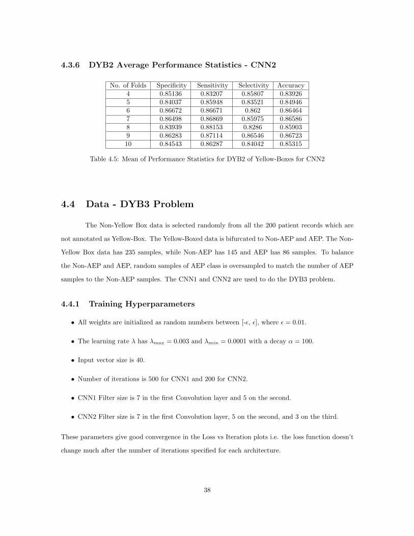
4.3.6 DYB2 Average Performance Statistics - CNN2
No. of Folds Specificity Sensitivity Selectivity Accuracy4 0.85136 0.83207 0.85807 0.839265 0.84037 0.85948 0.83521 0.849466 0.86672 0.86671 0.862 0.864647 0.86498 0.86869 0.85975 0.865868 0.83939 0.88153 0.8286 0.859039 0.86283 0.87114 0.86546 0.8672310 0.84543 0.86287 0.84042 0.85315
Table 4.5: Mean of Performance Statistics for DYB2 of Yellow-Boxes for CNN2
4.4 Data - DYB3 Problem
The Non-Yellow Box data is selected randomly from all the 200 patient records which are
not annotated as Yellow-Box. The Yellow-Boxed data is bifurcated to Non-AEP and AEP. The Non-
Yellow Box data has 235 samples, while Non-AEP has 145 and AEP has 86 samples. To balance
the Non-AEP and AEP, random samples of AEP class is oversampled to match the number of AEP
samples to the Non-AEP samples. The CNN1 and CNN2 are used to do the DYB3 problem.
4.4.1 Training Hyperparameters
• All weights are initialized as random numbers between [-ε, ε], where ε = 0.01.
• The learning rate λ has λmax = 0.003 and λmin = 0.0001 with a decay α = 100.
• Input vector size is 40.
• Number of iterations is 500 for CNN1 and 200 for CNN2.
• CNN1 Filter size is 7 in the first Convolution layer and 5 on the second.
• CNN2 Filter size is 7 in the first Convolution layer, 5 on the second, and 3 on the third.
These parameters give good convergence in the Loss vs Iteration plots i.e. the loss function doesn’t
change much after the number of iterations specified for each architecture.
38

4.4.2 DYB3 Results CNN1
This section includes only the average performance statistics on each fold. The plots of Loss
vs Iterations, and the confusion matrices pertaining to this section are included in the appendix
A.1.1
39
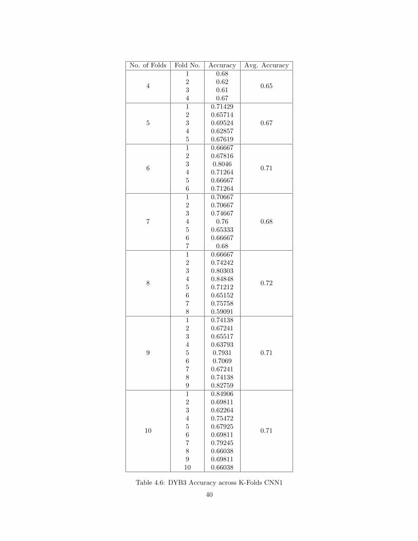
No. of Folds Fold No. Accuracy Avg. Accuracy
4
1 0.68
0.652 0.623 0.614 0.67
5
1 0.71429
0.672 0.657143 0.695244 0.628575 0.67619
6
1 0.66667
0.71
2 0.678163 0.80464 0.712645 0.666676 0.71264
7
1 0.70667
0.68
2 0.706673 0.746674 0.765 0.653336 0.666677 0.68
8
1 0.66667
0.72
2 0.742423 0.803034 0.848485 0.712126 0.651527 0.757588 0.59091
9
1 0.74138
0.71
2 0.672413 0.655174 0.637935 0.79316 0.70697 0.672418 0.741389 0.82759
10
1 0.84906
0.71
2 0.698113 0.622644 0.754725 0.679256 0.698117 0.792458 0.660389 0.6981110 0.66038
Table 4.6: DYB3 Accuracy across K-Folds CNN1
40

4.4.3 DYB3 Results CNN2
This section includes only the average performance statistics on each fold. The plots of Loss
vs Iterations, and the confusion matrices pertaining to this section are included in the appendix
A.1.2
41

No. of Folds Fold No. Accuracy Avg. Accuracy
4
1 0.76336
0.742 0.778633 0.770994 0.70229
5
1 0.71429
0.742 0.733333 0.742864 0.771435 0.74286
6
1 0.75862
0.75
2 0.724143 0.79314 0.747135 0.816096 0.67816
7
1 0.8
0.77
2 0.773333 0.786674 0.786675 0.706676 0.826677 0.76
8
1 0.87879
0.75
2 0.863643 0.696974 0.696975 0.742426 0.727277 0.772738 0.65152
9
1 0.77586
0.76
2 0.724143 0.775864 0.724145 0.79316 0.70697 0.810348 0.79319 0.77586
10
1 0.77358
0.76
2 0.849063 0.735854 0.754725 0.867926 0.716987 0.773588 0.754729 0.7358510 0.71698
Table 4.7: DYB3 Accuracy across K-Folds CNN2
42

4.5 Data - DYB5 Problem
From the table 2.2, it is observed that there is imbalance in the data amongst 201, 202,
204, 205 cases. Hence, the data is balanced by replication. Here, since the 201 and 204 cases have
samples much lesser than 202, all the cases are balanced by oversampling to match a mean length of
60 samples. 202 is kept at 106 samples. 60 samples of Non-Yellow boxes is also taken. The models
in this section classify the above data to Non-YB, 201, 202, 204, and 205 classes. CNN1 and CNN2
are used for this problem.
4.5.1 Training Hyperparameters
• All weights are initialized as random numbers between [-ε, ε], where ε = 0.01.
• The learning rate λ has λmax = 0.001 and λmin = 0.0001 with a decay α = 400.
• Input vector size is 40.
• Number of iterations is 1000 for CNN1 and 200 for CNN2.
• CNN1 Filter size is 7 in the first Convolution layer and 5 on the second.
• CNN2 Filter size is 7 in the first Convolution layer, 5 on the second, and 3 on the third.
These parameters give good convergence in the Loss vs Iteration plots i.e. the loss function doesn’t
change much after the number of iterations specified for each architecture.
4.5.2 DYB5 Results CNN1
This section includes only the average performance statistics on each fold. The plots of Loss
vs Iterations, and the confusion matrices pertaining to this section are included in the appendix
A.2.1
43
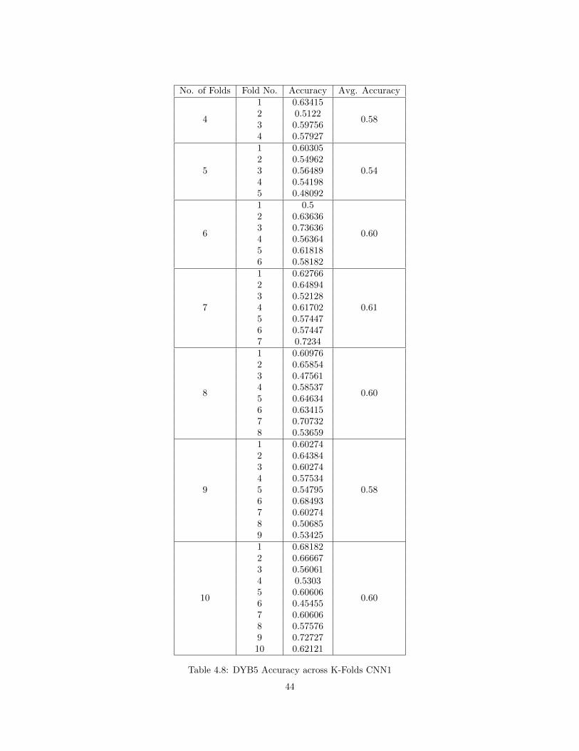
No. of Folds Fold No. Accuracy Avg. Accuracy
4
1 0.63415
0.582 0.51223 0.597564 0.57927
5
1 0.60305
0.542 0.549623 0.564894 0.541985 0.48092
6
1 0.5
0.60
2 0.636363 0.736364 0.563645 0.618186 0.58182
7
1 0.62766
0.61
2 0.648943 0.521284 0.617025 0.574476 0.574477 0.7234
8
1 0.60976
0.60
2 0.658543 0.475614 0.585375 0.646346 0.634157 0.707328 0.53659
9
1 0.60274
0.58
2 0.643843 0.602744 0.575345 0.547956 0.684937 0.602748 0.506859 0.53425
10
1 0.68182
0.60
2 0.666673 0.560614 0.53035 0.606066 0.454557 0.606068 0.575769 0.7272710 0.62121
Table 4.8: DYB5 Accuracy across K-Folds CNN1
44

4.5.3 DYB5 Results CNN2
This section includes only the average performance statistics on each fold. The plots of Loss
vs Iterations, and the confusion matrices pertaining to this section are included in the appendix
A.2.2
45

No. of Folds Fold No. Accuracy Avg. Accuracy
4
1 0.81098
0.792 0.823173 0.719514 0.81707
5
1 0.78626
0.822 0.816793 0.832064 0.847335 0.83969
6
1 0.84545
0.80
2 0.818183 0.818184 0.781825 0.763646 0.82727
7
1 0.73404
0.80
2 0.808513 0.744684 0.829795 0.819156 0.851067 0.82979
8
1 0.84146
0.82
2 0.792683 0.731714 0.817075 0.878056 0.853667 0.817078 0.85366
9
1 0.83562
0.82
2 0.753423 0.917814 0.849325 0.821926 0.821927 0.753428 0.808229 0.87671
10
1 0.83333
0.82
2 0.818183 0.757584 0.878795 0.924246 0.787887 0.727278 0.787889 0.9090910 0.84848
Table 4.9: DYB5 Accuracy across K-Folds CNN2
46

4.6 Conclusion
4.6.1 Conclusion for DYB2 Results
Both the CNN1 and CNN2 architectures return good results. The performance parameters
are fairly consistent with deviation less than 0.05 in Specificity, Sensitivity, and Selectivity across
the different K-fold validations. The CNN2 architecture has higher average accuracy as compared
to the CNN1. Although K = 9 shows the highest accuracy amongst the different K-folds in both the
tables 4.3 and 4.5, K = 6 shows similar characteristics in terms of accuracy and other performance
metrics. Also, K = 6 gives a good split of the available data into training and testing sets, which
has sufficient data for both training and testing and sufficient folds to consider averaging statistics
as a measure of performance analysis.
4.6.2 Conclusion for DYB3 Results
The average accuracy for CNN1 decreases by 10% as compared with the 2 class detection
results. The average accuracy for CNN2 decreases by 2% as compared with the 2 class detection
results. While CNN1 performs poorly in the DYB3, CNN2 performs consistently well detecting the
Non-Yellow-Boxes as well as classifying the Yellow-Boxes to Non-AEP and AEP.
4.6.3 Conclusion for DYB5 Results
The average accuracy for CNN1 and CNN2 both remain the same for DYB3 and DYB5
cases. CNN2 is very consistent across the K-folds as well and hence, it is better suited for multi-
class classification problems in this phase.
47
Chapter 5
Classification of Yellow-Boxes
CNN1 and CNN2 are trained to classify the annotated Yellow-Boxes. The Yellow-Boxed
data is classified separately into a 2 class and a 4 class problem. For the 2 class problem, the data is
classified into either a AEP or a Non-AEP. For a 4 class problem, the data is classified as per Table
2.1, discarding the 203 confidence level due to very low observations of that class. Also, the data is
not equally distributed among the classes, so it is balanced by random replication of cases to match
the cases observed for the highest annotated class for the 2 class case. For the 4 class case, the class
data is replicated to 60 values each, since replication to highest annotated class i.e. 106 is very high.
5.1 Approach
Both the CNN1 and CNN2 models are trained for this classification. The filter size is chosen
to be around 5-9 points, since the epileptic transient spikes are of length 20-70ms and with a 256Hz
sampling, it is appropriate to choose filters that encompass the transient spike activity length. The
input length is chosen to be around 40-80 points in length since most annotated events are of the
same length. A parameter search operation is done to estimate the best hyperparameters for the
convolution network architecture. It is found that the filter size of 7 with reductions of 2 in filtersize
per each convolution layer, and an input size of 40 points yield the highest accuracy in terms of
classification. Classification of Yellow-Boxes into Non-AEP and AEP is referred to as CYB2, and
classification into 201, 202, 204, and 205 is referred to as CYB4.
48

Figure 5.1: Block Diagram for CYB2 of Yellow-Box Network
Figure 5.2: Block Diagram for 4 Class Classification of Yellow-Box Network
5.2 CYB2 Problem
K-fold cross validation with K from 4 to 10 is performed on this data. Performance metrics
like Sensitivity, Specificity, Selectivity and Accuracy are calculated.
5.2.1 Training Hyperparameters
• All weights are initialized as random numbers between [-ε, ε], where ε = 0.01.
• The learning rate λ has λmax = 0.003 and λmin = 0.0003 with a decay α = 200.
• Input vector size is 40.
49
• Number of iterations is 500 for CNN1 and 200 for CNN2.
• CNN1 Filter size is 7 in the first Convolution layer and 5 on the second.
• CNN2 Filter size is 7 in the first Convolution layer, 5 on the second, and 3 on the third.
These parameters give good convergence in the Loss vs Iteration plots i.e. the loss function doesn’t
change much after the number of iterations specified for each architecture.
5.2.2 CYB2 Results - CNN1
This section includes the data split of Non-AEP and AEP samples, plots of Loss vs Iter-
ations for each fold of K-fold validation, performance metrics of the CNN1 architecture, average
performance over all the folds for each K in 4 to 10.
50

No. of Folds Fold No. No. of Non-AEP No. of AEP Ratio Non-AEP/AEP Total
4
1 38 35 1.0857 732 34 44 0.77273 783 39 34 1.1471 734 39 34 1.1471 73
5
1 23 35 0.65714 582 24 23 1.0435 473 24 34 0.70588 584 31 27 1.1481 585 27 31 0.87097 59
6
1 27 22 1.2273 492 22 27 0.81481 493 28 21 1.3333 494 24 25 0.96 495 23 26 0.88462 496 24 25 0.96 49
7
1 21 21 1 422 25 21 1.1905 463 18 24 0.75 424 23 19 1.2105 425 19 23 0.82609 426 17 25 0.68 427 12 30 0.4 42
8
1 23 14 1.6429 372 18 20 0.9 363 17 20 0.85 374 11 26 0.42308 375 18 19 0.94737 376 19 18 1.0556 377 18 19 0.94737 378 21 16 1.3125 37
9
1 12 21 0.57143 332 20 12 1.6667 323 14 19 0.73684 334 13 20 0.65 335 23 10 2.3 336 13 20 0.65 337 17 16 1.0625 318 15 18 0.83333 339 11 22 0.5 33
10
1 13 16 0.8125 292 9 15 0.6 243 12 17 0.70588 294 13 16 0.8125 295 7 22 0.31818 296 13 16 0.8125 297 11 18 0.61111 298 14 15 0.93333 299 18 11 1.6364 2910 18 11 1.6364 29
Table 5.1: Distribution of Data for CYB2 of Yellow-Boxes
51

0 50 100 150 200 250 300 350 400 450 500
Number of Iterations
0.6
0.7
0.8
0.9
1
1.1
1.2
Cro
ss E
ntro
py L
oss
Fold 1Fold 2Fold 3Fold 4
Figure 5.3: CYB2 K = 4 Validation. Loss vsIterations for CNN1 Architecture
0 50 100 150 200 250 300 350 400 450 500
Number of Iterations
0.6
0.7
0.8
0.9
1
1.1
1.2
Cro
ss E
ntro
py L
oss
Fold 1Fold 2Fold 3Fold 4Fold 5
Figure 5.4: CYB2 K = 5 Validation. Loss vsIterations for CNN1 Architecture
0 50 100 150 200 250 300 350 400 450 500
Number of Iterations
0.6
0.7
0.8
0.9
1
1.1
1.2
Cro
ss E
ntro
py L
oss
Fold 1Fold 2Fold 3Fold 4Fold 5Fold 6
Figure 5.5: CYB2 K = 6 Validation. Loss vsIterations for CNN1 Architecture
0 50 100 150 200 250 300 350 400 450 500
Number of Iterations
0.6
0.7
0.8
0.9
1
1.1
1.2
Cro
ss E
ntro
py L
oss
Fold 1Fold 2Fold 3Fold 4Fold 5Fold 6Fold 7
Figure 5.6: CYB2 K = 7 Validation. Loss vsIterations for CNN1 Architecture
52

0 50 100 150 200 250 300 350 400 450 500
Number of Iterations
0.6
0.7
0.8
0.9
1
1.1
1.2
Cro
ss E
ntro
py L
oss
Fold 1Fold 2Fold 3Fold 4Fold 5Fold 6Fold 7Fold 8
Figure 5.7: CYB2 K = 8 Validation. Loss vsIterations for CNN1 Architecture
0 50 100 150 200 250 300 350 400 450 500
Number of Iterations
0.5
0.6
0.7
0.8
0.9
1
1.1
1.2
Cro
ss E
ntro
py L
oss
Fold 1Fold 2Fold 3Fold 4Fold 5Fold 6Fold 7Fold 8Fold 9
Figure 5.8: CYB2 K = 9 Validation. Loss vsIterations for CNN1 Architecture
0 50 100 150 200 250 300 350 400 450 500
Number of Iterations
0.6
0.7
0.8
0.9
1
1.1
1.2
Cro
ss E
ntro
py L
oss
Fold 1Fold 2Fold 3Fold 4Fold 5Fold 6Fold 7Fold 8Fold 9Fold 10
Figure 5.9: CYB2 K = 10 Validation. Loss vs Iterations for CNN1 Architecture
53
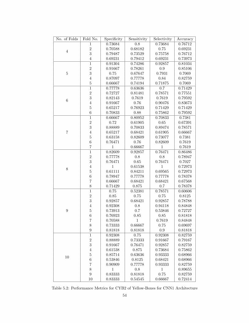
No. of Folds Fold No. Specificity Sensitivity Selectivity Accuracy
4
1 0.73684 0.8 0.73684 0.767122 0.70588 0.68182 0.75 0.692313 0.79487 0.73529 0.75758 0.767124 0.69231 0.79412 0.69231 0.73973
5
1 0.91304 0.74286 0.92857 0.810342 0.91667 0.78261 0.9 0.851063 0.75 0.67647 0.7931 0.70694 0.87097 0.77778 0.84 0.827595 0.66667 0.74194 0.71875 0.7069
6
1 0.77778 0.63636 0.7 0.714292 0.72727 0.81481 0.78571 0.775513 0.82143 0.7619 0.7619 0.795924 0.91667 0.76 0.90476 0.836735 0.65217 0.76923 0.71429 0.714296 0.70833 0.88 0.75862 0.79592
7
1 0.66667 0.80952 0.70833 0.73812 0.72 0.61905 0.65 0.673913 0.88889 0.70833 0.89474 0.785714 0.65217 0.68421 0.61905 0.666675 0.63158 0.82609 0.73077 0.73816 0.76471 0.76 0.82609 0.76197 1 0.66667 1 0.7619
8
1 0.82609 0.92857 0.76471 0.864862 0.77778 0.8 0.8 0.789473 0.76471 0.65 0.76471 0.70274 1 0.61538 1 0.729735 0.61111 0.84211 0.69565 0.729736 0.78947 0.77778 0.77778 0.783787 0.66667 0.68421 0.68421 0.675688 0.71429 0.875 0.7 0.78378
9
1 0.75 0.52381 0.78571 0.606062 0.85 0.75 0.75 0.81253 0.92857 0.68421 0.92857 0.787884 0.92308 0.8 0.94118 0.848485 0.73913 0.7 0.53846 0.727276 0.76923 0.85 0.85 0.818187 0.70588 1 0.7619 0.848488 0.73333 0.66667 0.75 0.696979 0.81818 0.81818 0.9 0.81818
10
1 0.92308 0.75 0.92308 0.827592 0.88889 0.73333 0.91667 0.791673 0.91667 0.76471 0.92857 0.827594 0.61538 0.875 0.73684 0.758625 0.85714 0.63636 0.93333 0.689666 0.53846 0.8125 0.68421 0.689667 0.90909 0.77778 0.93333 0.827598 1 0.8 1 0.896559 0.83333 0.81818 0.75 0.8275910 0.83333 0.54545 0.66667 0.72414
Table 5.2: Performance Metrics for CYB2 of Yellow-Boxes for CNN1 Architecture
54

5.2.3 CYB2 Average Performance Statistics - CNN1
No. of Folds Specificity Sensitivity Selectivity Accuracy
4 0.73248 0.75281 0.73418 0.74157
5 0.82347 0.74433 0.83608 0.78056
6 0.76728 0.77039 0.77088 0.77211
7 0.76057 0.72484 0.77557 0.73233
8 0.76876 0.77163 0.77338 0.75747
9 0.80193 0.75476 0.80065 0.77378
10 0.83154 0.75133 0.84727 0.78606
Table 5.3: Mean of Performance Statistics for CYB2 of Yellow-Boxes CNN1
55

5.2.4 CYB2 Results - CNN2
This section includes the plots of Loss vs Iterations for each fold of K-fold validation, per-
formance metrics of the CNN1 architecture, average performance over all the folds for each K in 4
to 10.
0 20 40 60 80 100 120 140 160 180 200
Number of Iterations
0
20
40
60
80
100
120
140
160
Cro
ss E
ntro
py L
oss
Fold 1Fold 2Fold 3Fold 4
Figure 5.10: CYB2 K = 4 Validation. Loss vsIterations for CNN2 Architecture
0 20 40 60 80 100 120 140 160 180 200
Number of Iterations
0
20
40
60
80
100
120
140
160
180
200
Cro
ss E
ntro
py L
oss
Fold 1Fold 2Fold 3Fold 4Fold 5
Figure 5.11: CYB2 K = 5 Validation. Loss vsIterations for CNN2 Architecture
0 20 40 60 80 100 120 140 160 180 200
Number of Iterations
0
20
40
60
80
100
120
Cro
ss E
ntro
py L
oss
Fold 1Fold 2Fold 3Fold 4Fold 5Fold 6
Figure 5.12: CYB2 K = 6 Validation. Loss vsIterations for CNN2 Architecture
0 20 40 60 80 100 120 140 160 180 200
Number of Iterations
0
20
40
60
80
100
120
140
Cro
ss E
ntro
py L
oss
Fold 1Fold 2Fold 3Fold 4Fold 5Fold 6Fold 7
Figure 5.13: CYB2 K = 7 Validation. Loss vsIterations for CNN2 Architecture
56
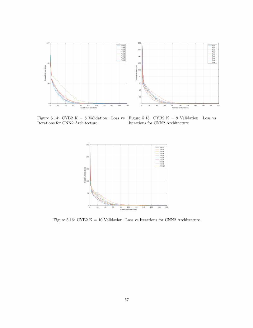
0 20 40 60 80 100 120 140 160 180 200
Number of Iterations
0
50
100
150C
ross
Ent
ropy
Los
sFold 1Fold 2Fold 3Fold 4Fold 5Fold 6Fold 7Fold 8
Figure 5.14: CYB2 K = 8 Validation. Loss vsIterations for CNN2 Architecture
0 20 40 60 80 100 120 140 160 180 200
Number of Iterations
0
20
40
60
80
100
120
140
160
180
Cro
ss E
ntro
py L
oss
Fold 1Fold 2Fold 3Fold 4Fold 5Fold 6Fold 7Fold 8Fold 9
Figure 5.15: CYB2 K = 9 Validation. Loss vsIterations for CNN2 Architecture
0 20 40 60 80 100 120 140 160 180 200
Number of Iterations
0
50
100
150
200
250
Cro
ss E
ntro
py L
oss
Fold 1Fold 2Fold 3Fold 4Fold 5Fold 6Fold 7Fold 8Fold 9Fold 10
Figure 5.16: CYB2 K = 10 Validation. Loss vs Iterations for CNN2 Architecture
57

No. of Folds Fold No. Specificity Sensitivity Selectivity Accuracy
4
1 0.86486 0.86111 0.86111 0.863012 0.84375 0.75 0.85714 0.791673 0.85294 0.76923 0.85714 0.808224 0.88235 0.92308 0.9 0.90411
5
1 0.92593 0.87097 0.93103 0.896552 0.9 0.81818 0.93103 0.849063 0.87879 0.92 0.85185 0.896554 0.96154 0.84375 0.96429 0.896555 0.80769 0.6875 0.81481 0.74138
6
1 0.88889 0.74194 0.92 0.795922 0.90909 0.82609 0.90476 0.866673 0.90909 0.85185 0.92 0.877554 0.91667 0.88 0.91667 0.897965 1 0.85185 1 0.918376 0.91667 0.88 0.91667 0.89796
7
1 0.9 0.86364 0.90476 0.880952 0.88889 0.68 0.89474 0.767443 1 0.90476 1 0.952384 0.95238 0.85714 0.94737 0.904765 0.83333 0.875 0.875 0.857146 0.875 0.84615 0.91667 0.857147 0.94118 0.84 0.95455 0.88095
8
1 1 0.91304 1 0.945952 1 0.85 1 0.918923 0.76471 0.7 0.77778 0.729734 0.9375 0.71429 0.9375 0.810815 0.8 0.90909 0.86957 0.864866 0.84211 0.72222 0.8125 0.783787 1 0.9375 1 0.972978 0.83333 0.84 0.91304 0.83784
9
1 1 0.94737 1 0.96972 1 0.82353 1 0.909093 0.92308 0.9 0.94737 0.909094 1 0.68182 1 0.787885 1 0.77778 1 0.878796 0.8 0.83333 0.83333 0.818187 1 0.85 1 0.909098 0.73333 0.77778 0.77778 0.757589 1 0.88889 1 0.93939
10
1 0.81818 0.88889 0.88889 0.862072 0.88235 0.83333 0.83333 0.862073 0.875 0.92308 0.85714 0.896554 0.92308 0.75 0.92308 0.827595 0.94444 0.81818 0.9 0.896556 0.75 0.76471 0.8125 0.758627 0.85714 0.93333 0.875 0.896558 0.66667 0.70588 0.75 0.689669 1 0.7 1 0.793110 0.85714 0.93333 0.875 0.89655
Table 5.4: Performance Metrics for CYB2 of Yellow-Boxes for CNN2 Architecture
58
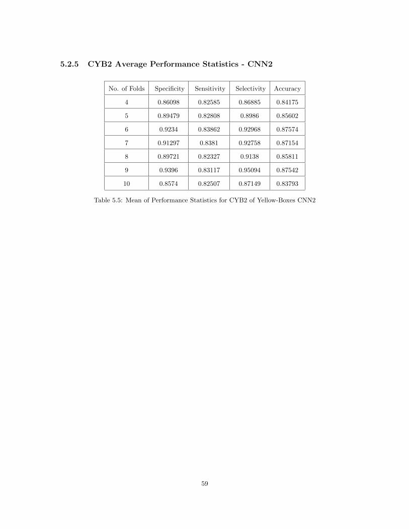
5.2.5 CYB2 Average Performance Statistics - CNN2
No. of Folds Specificity Sensitivity Selectivity Accuracy
4 0.86098 0.82585 0.86885 0.84175
5 0.89479 0.82808 0.8986 0.85602
6 0.9234 0.83862 0.92968 0.87574
7 0.91297 0.8381 0.92758 0.87154
8 0.89721 0.82327 0.9138 0.85811
9 0.9396 0.83117 0.95094 0.87542
10 0.8574 0.82507 0.87149 0.83793
Table 5.5: Mean of Performance Statistics for CYB2 of Yellow-Boxes CNN2
59

5.3 CYB4 Problem
From Table 2.2, it is observed that there is imbalance in the data amongst 201, 202, 204, 205
cases. Hence, the data is balanced by replication. Here, since the 201 and 204 cases have samples
much lesser than 202, all the cases are balanced by replication to match a mean length of 60 samples.
202 is reduced to 60 samples. The models in this section classify the above data 201, 202, 204, and
205 classes. CNN1 and CNN2 are used for this classification problem.
5.3.1 Training Hyperparameters
• All weights are initialized as random numbers between [-ε, ε], where ε = 0.01.
• The learning rate λ has λmax = 0.003 and λmin = 0.0001 with a decay α = 200.
• Input vector size is 40.
• Number of iterations is 1000 for CNN1 and 200 for CNN2.
• CNN1 Filter size is 7 in the first Convolution layer and 5 on the second.
• CNN2 Filter size is 7 in the first Convolution layer, 5 on the second, and 3 on the third.
5.3.2 CYB4 Results CNN1
This section includes only the average performance statistics on each fold. The plots of Loss
vs Iterations, and the confusion matrices pertaining to this section are included in the appendix B.1
60
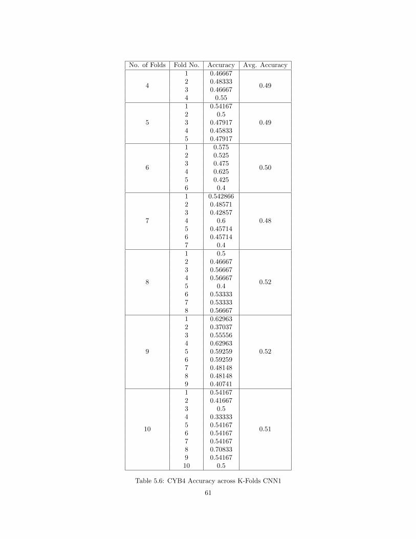
No. of Folds Fold No. Accuracy Avg. Accuracy
4
1 0.46667
0.492 0.483333 0.466674 0.55
5
1 0.54167
0.492 0.53 0.479174 0.458335 0.47917
6
1 0.575
0.50
2 0.5253 0.4754 0.6255 0.4256 0.4
7
1 0.542866
0.48
2 0.485713 0.428574 0.65 0.457146 0.457147 0.4
8
1 0.5
0.52
2 0.466673 0.566674 0.566675 0.46 0.533337 0.533338 0.56667
9
1 0.62963
0.52
2 0.370373 0.555564 0.629635 0.592596 0.592597 0.481488 0.481489 0.40741
10
1 0.54167
0.51
2 0.416673 0.54 0.333335 0.541676 0.541677 0.541678 0.708339 0.5416710 0.5
Table 5.6: CYB4 Accuracy across K-Folds CNN1
61

5.3.3 CYB4 Results CNN2
This section includes only the average performance statistics on each fold. The plots of Loss
vs Iterations, and the confusion matrices pertaining to this section are included in the appendix
B.1.1
62
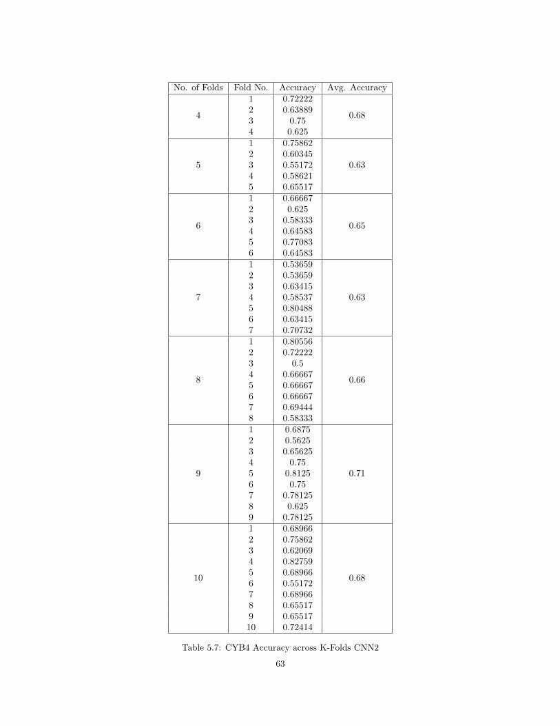
No. of Folds Fold No. Accuracy Avg. Accuracy
4
1 0.72222
0.682 0.638893 0.754 0.625
5
1 0.75862
0.632 0.603453 0.551724 0.586215 0.65517
6
1 0.66667
0.65
2 0.6253 0.583334 0.645835 0.770836 0.64583
7
1 0.53659
0.63
2 0.536593 0.634154 0.585375 0.804886 0.634157 0.70732
8
1 0.80556
0.66
2 0.722223 0.54 0.666675 0.666676 0.666677 0.694448 0.58333
9
1 0.6875
0.71
2 0.56253 0.656254 0.755 0.81256 0.757 0.781258 0.6259 0.78125
10
1 0.68966
0.68
2 0.758623 0.620694 0.827595 0.689666 0.551727 0.689668 0.655179 0.6551710 0.72414
Table 5.7: CYB4 Accuracy across K-Folds CNN2
63
5.4 Conclusion
5.4.1 Conclusion for CYB2 Results
Tables 5.3 and 5.5 show the convolution neural network models perform well. CNN1 has an
76% classification accuracy with consistent specificity, selectivity, sensitivity. The CNN2 averages
at 85% accuracy and is also very consistent with the performance metrics. CNN2 records a 10%
positive shift in all the performance metrics as compared to CNN1. K = 5 for CNN1 and K = 6 for
CNN2 give the highest percent accuracy in classification.
5.4.2 Conclusion for CYB4 Results
The CNN1 accuracy decreases by more than 25% as compared to the CYB2 Results. This
fall in accuracy is only 10% for the DYB3 results. Similarly, the accuracy for CNN2 also falls down
by 25% as compared to the CYB2 Results. This fall in accuracy characterizes that the intra-class
classification amongst the Yellow-Boxed results is more intricate as compared to classifying Non-
Yellow and Yellow-Boxes. K = 8 for CNN1 and K = 9 for CNN2 show the highest accuracy in terms
of classification.
64

Chapter 6
Overall System Validation
The objective of this thesis is to have an end-to-end deep learning ET detector and classifier.
This is achieved individually in the previous sections. The overall system can be done in 3 different
ways. Figures 4.1, 4.2, and 4.3 show the models for overall system validation. Only CNN2 is used
for system validation as it has higher classification accuracy in both the detection and classification
phases.
6.1 Data
For the model shown in fig. 4.1, two separate CNN2s are trained, one for detection of
Yellow-Boxes and the other for Classification of detected boxes. For the models shown in the figures
4.2, and 4.3, only one CNN2 is trained. A selection of 7 EEG signals is chosen with high number of
annotations by the neurologists followed by 3 signals chosen randomly from the set of Non-ET signals
is put together as the validation set for these models. Unlike in the detection and the classification
phase, the validation set signals are entire EEG signals that are input to the models. The data
selected has the following characteristics: The data from each of these signals is fed to the models as
segments of 40 points each. There is an overlap of 25% for each successive input segment of 40 points.
Each of the signals in the table 6.1 is extracted from a specific montage, some of the annotations
made are from different montages. Hence, the highest number of annotations for a single montage
is selected and the EEG of that montage is extracted for a particular signal in the validation set.
To visualize the results, the ground truth is marked with yellow and green boxes for Non-
65

Signal No. Montage ID No. YB No. of 201 No. of 202 No. of 204 No. of 20512 11 7 1 2 4 030 10 6 3 3 0 036 17 8 0 0 0 865 10 12 0 0 0 1289 10 10 0 0 0 1095 10 7 0 4 0 3160 11 7 0 4 3 034 10 0 No Epileptiform Transients93 10 0 No Epileptiform Transients194 10 0 No Epileptiform Transients
Table 6.1: Table showing the Validation Set
AEP and AEP respectively, while the classifier predicted output is marked with black and red boxes
for Non-AEP and AEP.
6.2 Performance Measures
Each EEG segment in the validation set is 30s in length, sampled at 256Hz. This implies the
length of each segment is 7680 points, while the input size is only 40 points each. Hence, the usual
performance metrics like sensitivity, selectivity and specificity are not the ideal metrics to evaluate
the system. For classification strategies marking segments in a time series data, a good performance
metric would be measuring ratio of the length of segments marked to groundtruth lengths. The two
performance metrics defined below use this statistic:
• Marking Ratio (M): The Marking ratio is the length of the signals marked to the length of the
total signal. An EEG signal with no ETs should have a marking ratio 0.
M =
∑Total Length of PredictedMarkedSignal
Total Length of theEEGSignal(6.1)
• Marking Hit Ratio(MH): The Marking hit ratio is the length of correctly marked signals to
the length of the marked signal from groundtruth. For a good detection system, MH Ratio is
1.
MH =
∑Total Length of Correctly PredictedMarkedSignals∑
Total Length of theGroundtruthMarking(6.2)
66
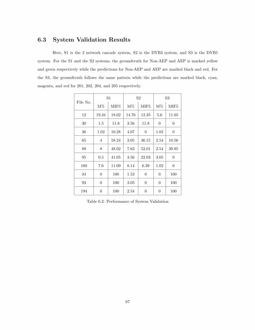
6.3 System Validation Results
Here, S1 is the 2 network cascade system, S2 is the DYB3 system, and S3 is the DYB5
system. For the S1 and the S2 systems, the groundtruth for Non-AEP and AEP is marked yellow
and green respectively while the predictions for Non-AEP and AEP are marked black and red. For
the S3, the groundtruth follows the same pattern while the predictions are marked black, cyan,
magenta, and red for 201, 202, 204, and 205 respectively.
File No.S1 S2 S3
M% MH% M% MH% M% MH%
12 19.34 18.02 14.76 12.35 5.6 11.05
30 1.5 11.8 3.56 11.8 0 0
36 1.02 10.28 4.07 0 1.02 0
65 4 58.24 3.05 36.15 2.54 10.56
89 8 48.02 7.63 52.01 2.54 39.95
95 0.5 41.05 3.56 22.03 3.05 0
160 7.6 11.09 8.14 6.39 1.02 0
34 0 100 1.53 0 0 100
93 0 100 3.05 0 0 100
194 0 100 2.54 0 0 100
Table 6.2: Performance of System Validation
67
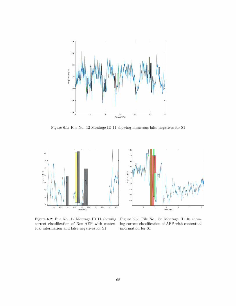
Figure 6.1: File No. 12 Montage ID 11 showing numerous false negatives for S1
Figure 6.2: File No. 12 Montage ID 11 showingcorrect classification of Non-AEP with contex-tual information and false negatives for S1
Figure 6.3: File No. 65 Montage ID 10 show-ing correct classification of AEP with contextualinformation for S1
68
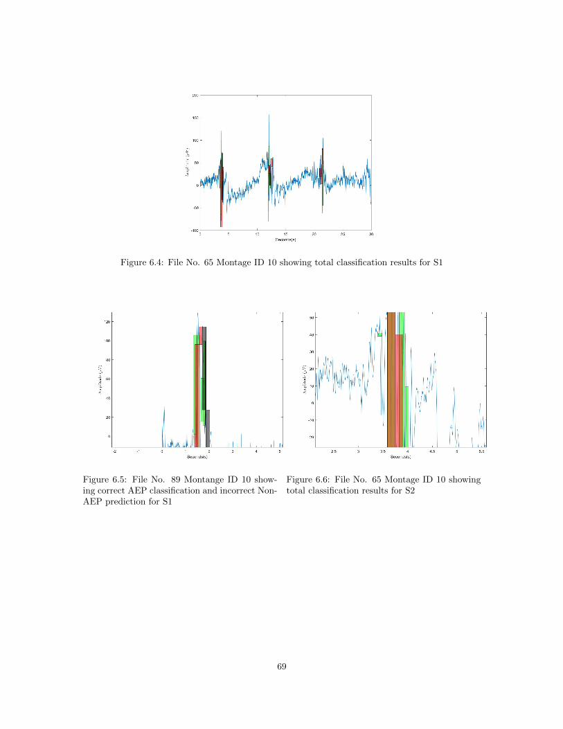
Figure 6.4: File No. 65 Montage ID 10 showing total classification results for S1
Figure 6.5: File No. 89 Montange ID 10 show-ing correct AEP classification and incorrect Non-AEP prediction for S1
Figure 6.6: File No. 65 Montage ID 10 showingtotal classification results for S2
69
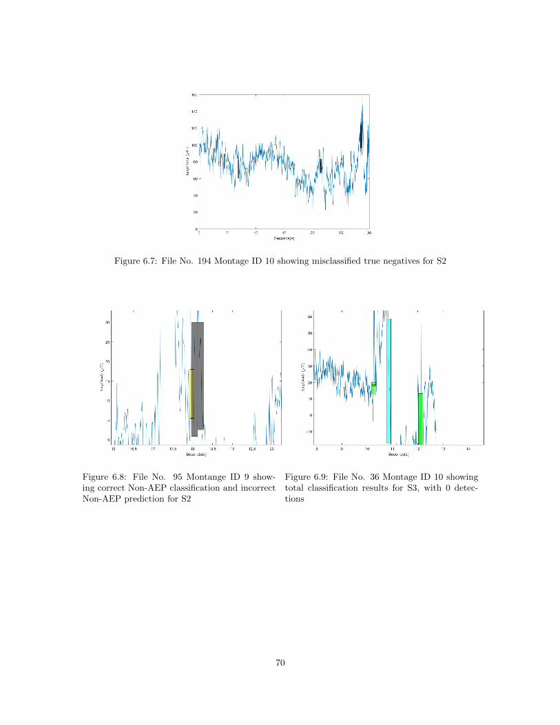
Figure 6.7: File No. 194 Montage ID 10 showing misclassified true negatives for S2
Figure 6.8: File No. 95 Montange ID 9 show-ing correct Non-AEP classification and incorrectNon-AEP prediction for S2
Figure 6.9: File No. 36 Montage ID 10 showingtotal classification results for S3, with 0 detec-tions
70

0 5 10 15 20 25 30
Seconds(s)
-150
-100
-50
0
50
100
Figure 6.10: File No. 93 Montage ID 10 showing perfect classification for S3
Figure 6.11: File No. 65 Montange ID 9 showingcorrect AEP Classification with contextual infor-mation for S3
Figure 6.12: File No. 65 Montage ID 10 showingtotal classification results for S3
71
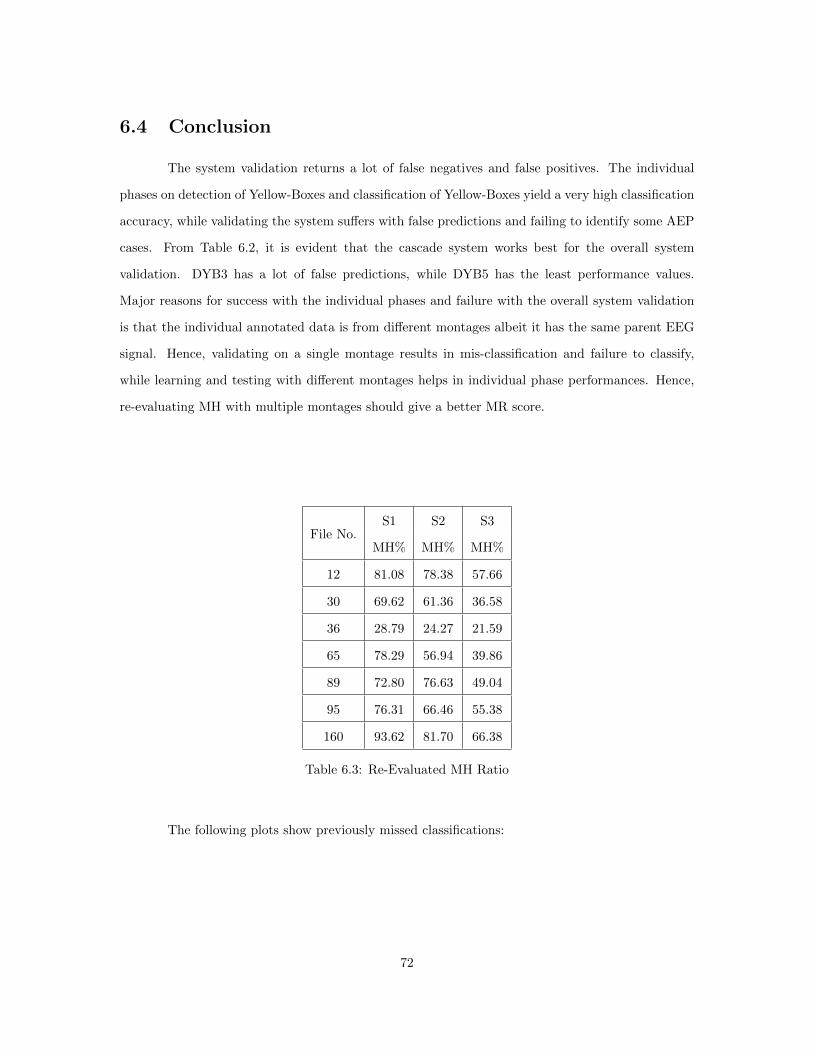
6.4 Conclusion
The system validation returns a lot of false negatives and false positives. The individual
phases on detection of Yellow-Boxes and classification of Yellow-Boxes yield a very high classification
accuracy, while validating the system suffers with false predictions and failing to identify some AEP
cases. From Table 6.2, it is evident that the cascade system works best for the overall system
validation. DYB3 has a lot of false predictions, while DYB5 has the least performance values.
Major reasons for success with the individual phases and failure with the overall system validation
is that the individual annotated data is from different montages albeit it has the same parent EEG
signal. Hence, validating on a single montage results in mis-classification and failure to classify,
while learning and testing with different montages helps in individual phase performances. Hence,
re-evaluating MH with multiple montages should give a better MR score.
File No.S1 S2 S3
MH% MH% MH%
12 81.08 78.38 57.66
30 69.62 61.36 36.58
36 28.79 24.27 21.59
65 78.29 56.94 39.86
89 72.80 76.63 49.04
95 76.31 66.46 55.38
160 93.62 81.70 66.38
Table 6.3: Re-Evaluated MH Ratio
The following plots show previously missed classifications:
72
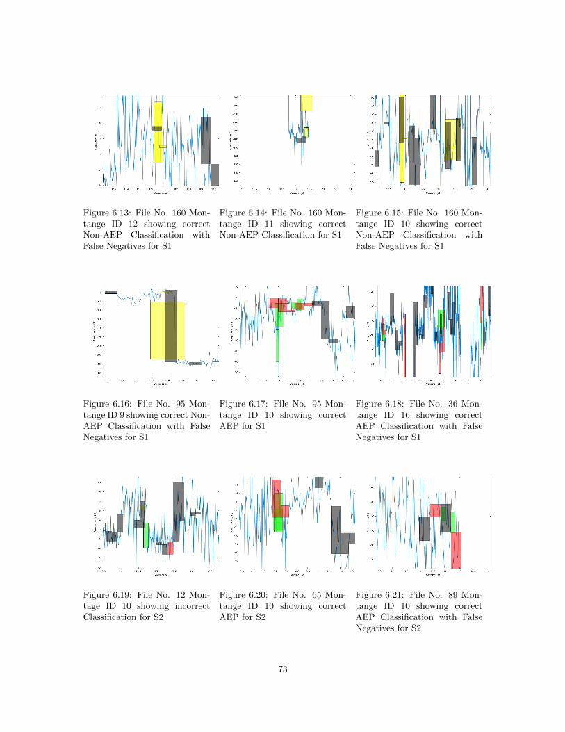
Figure 6.13: File No. 160 Mon-tange ID 12 showing correctNon-AEP Classification withFalse Negatives for S1
Figure 6.14: File No. 160 Mon-tange ID 11 showing correctNon-AEP Classification for S1
Figure 6.15: File No. 160 Mon-tange ID 10 showing correctNon-AEP Classification withFalse Negatives for S1
Figure 6.16: File No. 95 Mon-tange ID 9 showing correct Non-AEP Classification with FalseNegatives for S1
Figure 6.17: File No. 95 Mon-tange ID 10 showing correctAEP for S1
Figure 6.18: File No. 36 Mon-tange ID 16 showing correctAEP Classification with FalseNegatives for S1
Figure 6.19: File No. 12 Mon-tage ID 10 showing incorrectClassification for S2
Figure 6.20: File No. 65 Mon-tange ID 10 showing correctAEP for S2
Figure 6.21: File No. 89 Mon-tange ID 10 showing correctAEP Classification with FalseNegatives for S2
73

Figure 6.22: File No. 65 Mon-tage ID 10 showing Correct 204and 205 Classification for S3
Figure 6.23: File No. 89 Mon-tange ID 10 showing correct 204classification and incorrect 205detection for S3
Figure 6.24: File No. 160 Mon-tange ID 9 showing correct 201and 202 classification for S3
Since, the training accuracy for CNN2 is always near 100% for all cases, models based on
CNN2 should have a high MH score. The re-evaluation strategy accounts for all the montages that a
signal is annotated in, giving the models higher accuracy in determining all the Yellow-Boxed events
and classifying them. Even after re-evaluation the cascade system works best followed by DYB3 and
DYB5.
74
Chapter 7
Conclusion and Future Research
This thesis proposes 1-D Convolution Neural Network models to detect and classify Epileptic
Transients in EEG data. This is an end-to-end model, which by-passes the conventional feature
extraction step. The highest accuracy in terms of detection of yellow boxes is 93.84% for the CNN2
architecture with K = 9 (Table 4.4), and for classification of yellow boxes, it is 95.23% for K = 7
(Table 5.4). The over-all system performance is largely effected by false positives and false negatives,
while the system does a very good job in detecting true positives and negatives. The evaluation of
system performance with multiple montages boosts the true positive and negative detection. Table
7.1 summarizes all the cases considered in detection of Yellow-Boxes, Classification of Yellow-Boxes
and the over-all system validation.
While the results are promising, CNN1 and CNN2 architectures are quite shallow models.
Typical deep learning CNNs have 5-10 convolution layers at a minimum. Deep learning algorithms
take advantage of massive datasets, creating a layered, hierarchal architecture of learning and rep-
resenting data. The reason for CNN1 and CNN2 to be only 2 or 3 layers deep, is the limited
data available for this undertaking. A deeper neural network with limited data is prone to memo-
rize/overfitt the input data, and it may not be possible to train a deep network which generalizes
well. A shallower network architecture with normalization and dropout works quite well with limited
data.
75
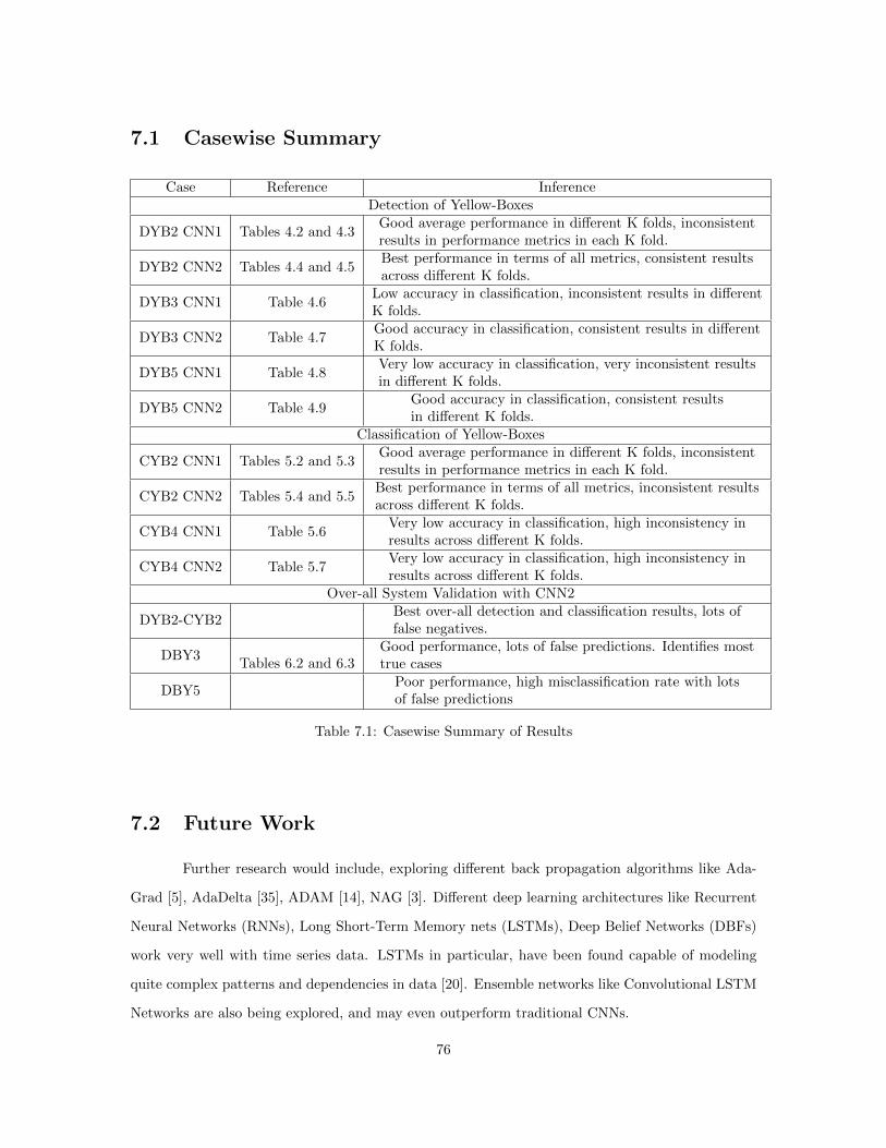
7.1 Casewise Summary
Case Reference InferenceDetection of Yellow-Boxes
DYB2 CNN1 Tables 4.2 and 4.3Good average performance in different K folds, inconsistentresults in performance metrics in each K fold.
DYB2 CNN2 Tables 4.4 and 4.5Best performance in terms of all metrics, consistent resultsacross different K folds.
DYB3 CNN1 Table 4.6Low accuracy in classification, inconsistent results in differentK folds.
DYB3 CNN2 Table 4.7Good accuracy in classification, consistent results in differentK folds.
DYB5 CNN1 Table 4.8Very low accuracy in classification, very inconsistent resultsin different K folds.
DYB5 CNN2 Table 4.9Good accuracy in classification, consistent resultsin different K folds.
Classification of Yellow-Boxes
CYB2 CNN1 Tables 5.2 and 5.3Good average performance in different K folds, inconsistentresults in performance metrics in each K fold.
CYB2 CNN2 Tables 5.4 and 5.5Best performance in terms of all metrics, inconsistent resultsacross different K folds.
CYB4 CNN1 Table 5.6Very low accuracy in classification, high inconsistency inresults across different K folds.
CYB4 CNN2 Table 5.7Very low accuracy in classification, high inconsistency inresults across different K folds.
Over-all System Validation with CNN2
DYB2-CYB2
Tables 6.2 and 6.3
Best over-all detection and classification results, lots offalse negatives.
DBY3Good performance, lots of false predictions. Identifies mosttrue cases
DBY5Poor performance, high misclassification rate with lotsof false predictions
Table 7.1: Casewise Summary of Results
7.2 Future Work
Further research would include, exploring different back propagation algorithms like Ada-
Grad [5], AdaDelta [35], ADAM [14], NAG [3]. Different deep learning architectures like Recurrent
Neural Networks (RNNs), Long Short-Term Memory nets (LSTMs), Deep Belief Networks (DBFs)
work very well with time series data. LSTMs in particular, have been found capable of modeling
quite complex patterns and dependencies in data [20]. Ensemble networks like Convolutional LSTM
Networks are also being explored, and may even outperform traditional CNNs.
76
Appendices
77
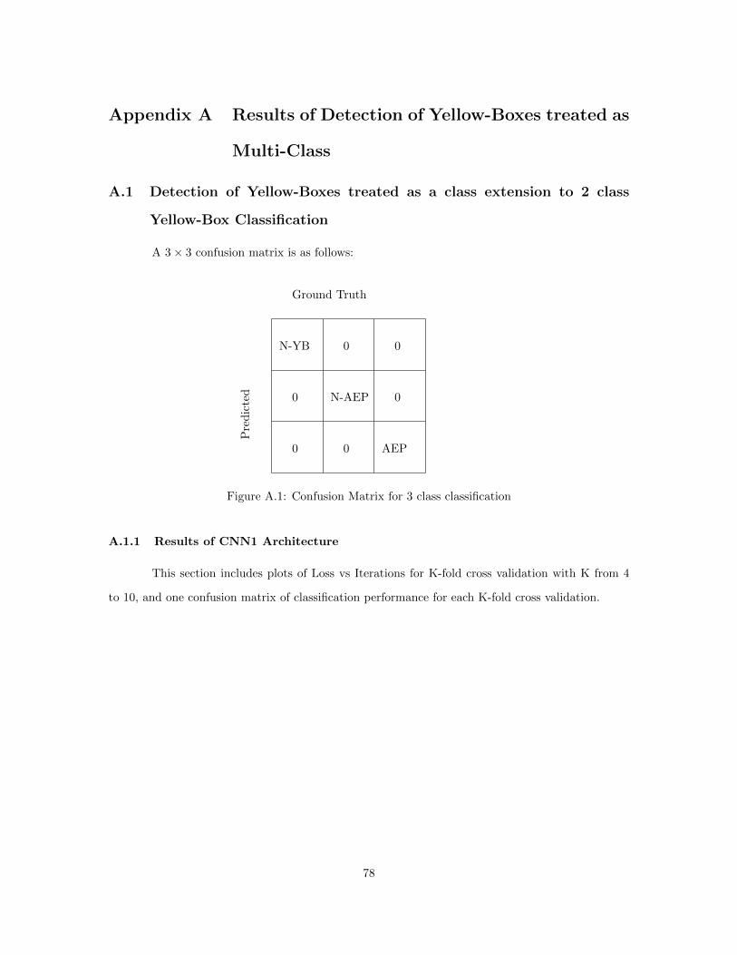
Appendix A Results of Detection of Yellow-Boxes treated as
Multi-Class
A.1 Detection of Yellow-Boxes treated as a class extension to 2 class
Yellow-Box Classification
A 3× 3 confusion matrix is as follows:
0 0 AEP
0 N-AEP 0
N-YB 0 0
Pre
dic
ted
Ground Truth
Figure A.1: Confusion Matrix for 3 class classification
A.1.1 Results of CNN1 Architecture
This section includes plots of Loss vs Iterations for K-fold cross validation with K from 4
to 10, and one confusion matrix of classification performance for each K-fold cross validation.
78
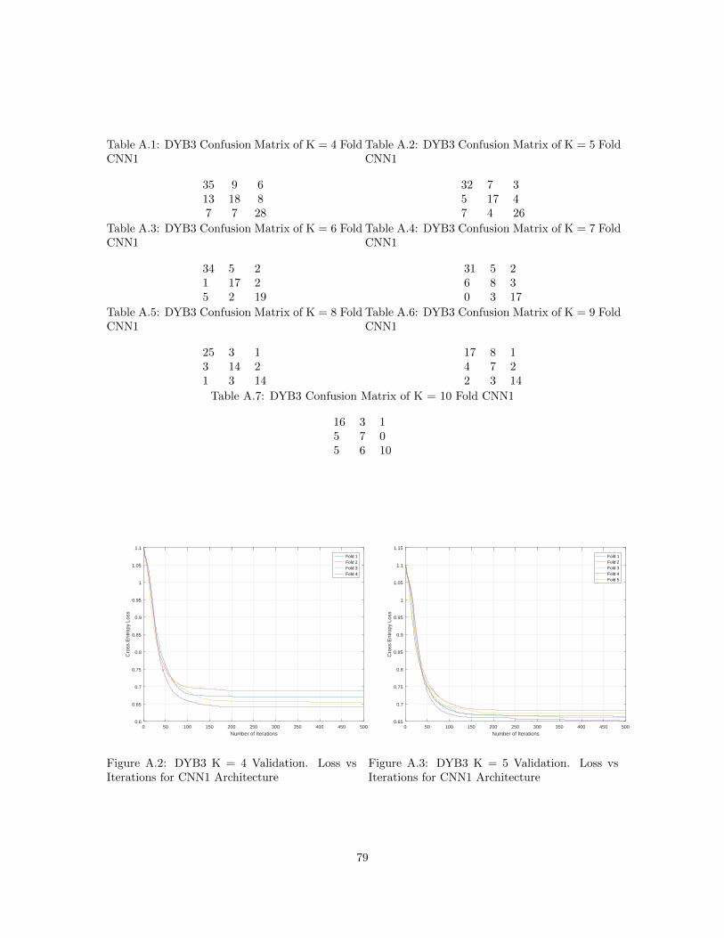
Table A.1: DYB3 Confusion Matrix of K = 4 FoldCNN1
35 9 613 18 87 7 28
Table A.2: DYB3 Confusion Matrix of K = 5 FoldCNN1
32 7 35 17 47 4 26
Table A.3: DYB3 Confusion Matrix of K = 6 FoldCNN1
34 5 21 17 25 2 19
Table A.4: DYB3 Confusion Matrix of K = 7 FoldCNN1
31 5 26 8 30 3 17
Table A.5: DYB3 Confusion Matrix of K = 8 FoldCNN1
25 3 13 14 21 3 14
Table A.6: DYB3 Confusion Matrix of K = 9 FoldCNN1
17 8 14 7 22 3 14
Table A.7: DYB3 Confusion Matrix of K = 10 Fold CNN1
16 3 15 7 05 6 10
0 50 100 150 200 250 300 350 400 450 500
Number of Iterations
0.6
0.65
0.7
0.75
0.8
0.85
0.9
0.95
1
1.05
1.1
Cro
ss E
ntro
py L
oss
Fold 1Fold 2Fold 3Fold 4
Figure A.2: DYB3 K = 4 Validation. Loss vsIterations for CNN1 Architecture
0 50 100 150 200 250 300 350 400 450 500
Number of Iterations
0.65
0.7
0.75
0.8
0.85
0.9
0.95
1
1.05
1.1
1.15
Cro
ss E
ntro
py L
oss
Fold 1Fold 2Fold 3Fold 4Fold 5
Figure A.3: DYB3 K = 5 Validation. Loss vsIterations for CNN1 Architecture
79

0 50 100 150 200 250 300 350 400 450 500
Number of Iterations
0.6
0.7
0.8
0.9
1
1.1
1.2
Cro
ss E
ntro
py L
oss
Fold 1Fold 2Fold 3Fold 4Fold 5Fold 6
Figure A.4: DYB3 K = 6 Validation. Loss vsIterations for CNN1 Architecture
0 50 100 150 200 250 300 350 400 450 500
Number of Iterations
0.65
0.7
0.75
0.8
0.85
0.9
0.95
1
1.05
1.1
1.15
Cro
ss E
ntro
py L
oss
Fold 1Fold 2Fold 3Fold 4Fold 5Fold 6Fold 7
Figure A.5: DYB3 K = 7 Validation. Loss vsIterations for CNN1 Architecture
0 50 100 150 200 250 300 350 400 450 500
Number of Iterations
0.6
0.7
0.8
0.9
1
1.1
1.2
Cro
ss E
ntro
py L
oss
Fold 1Fold 2Fold 3Fold 4Fold 5Fold 6Fold 7Fold 8
Figure A.6: DYB3 K = 8 Validation. Loss vsIterations for CNN1 Architecture
0 50 100 150 200 250 300 350 400 450 500
Number of Iterations
0.6
0.7
0.8
0.9
1
1.1
1.2
Cro
ss E
ntro
py L
oss
Fold 1Fold 2Fold 3Fold 4Fold 5Fold 6Fold 7Fold 8Fold 9
Figure A.7: DYB3 K = 9 Validation. Loss vsIterations for CNN1 Architecture
80
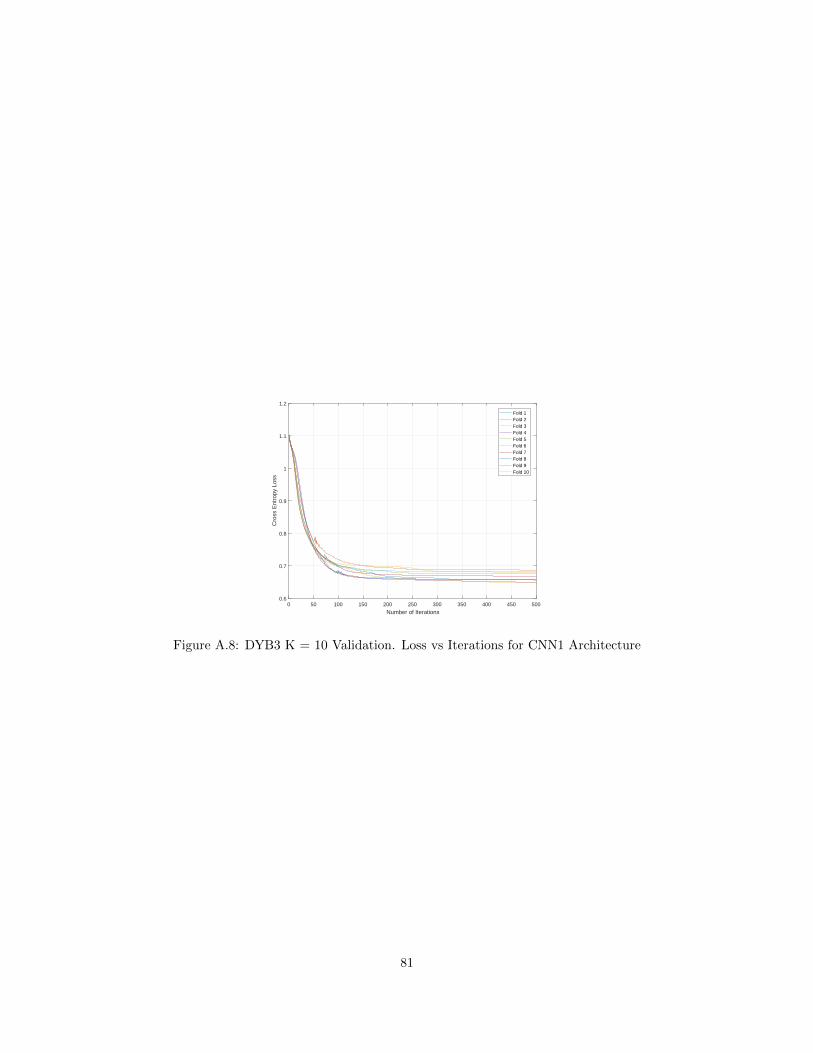
0 50 100 150 200 250 300 350 400 450 500
Number of Iterations
0.6
0.7
0.8
0.9
1
1.1
1.2
Cro
ss E
ntro
py L
oss
Fold 1Fold 2Fold 3Fold 4Fold 5Fold 6Fold 7Fold 8Fold 9Fold 10
Figure A.8: DYB3 K = 10 Validation. Loss vs Iterations for CNN1 Architecture
81

A.1.2 Results of CNN2 Architecture
This section includes plots of Loss vs Iterations for K-fold cross validation with K from 4
to 10, and one confusion matrix of classification performance for each K-fold cross validation.
Table A.8: DYB3 Confusion Matrix of K = 4 FoldCNN2
61 10 4
7 19 4
2 3 21
Table A.9: DYB3 Confusion Matrix of K = 5 FoldCNN2
46 11 0
5 15 1
0 7 20
Table A.10: DYB3 Confusion Matrix of K = 6Fold CNN2
37 6 1
1 13 4
1 3 21
Table A.11: DYB3 Confusion Matrix of K = 7Fold CNN2
28 6 0
4 14 0
1 2 20
Table A.12: DYB3 Confusion Matrix of K = 8Fold CNN2
27 3 1
3 9 0
0 1 22
Table A.13: DYB3 Confusion Matrix of K = 9Fold CNN2
23 2 0
6 9 2
0 1 15
Table A.14: DYB3 Confusion Matrix of K = 10 Fold CNN2
18 4 1
1 10 0
0 1 18
82
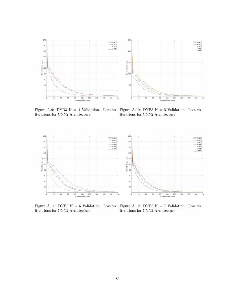
0 20 40 60 80 100 120 140 160 180 200
Number of Iterations
0
20
40
60
80
100
120
140
160
180
200C
ross
Ent
ropy
Los
sFold 1Fold 2Fold 3Fold 4
Figure A.9: DYB3 K = 4 Validation. Loss vsIterations for CNN2 Architecture
0 20 40 60 80 100 120 140 160 180 200
Number of Iterations
0
50
100
150
200
250
Cro
ss E
ntro
py L
oss
Fold 1Fold 2Fold 3Fold 4Fold 5
Figure A.10: DYB3 K = 5 Validation. Loss vsIterations for CNN2 Architecture
0 20 40 60 80 100 120 140 160 180 200
Number of Iterations
0
20
40
60
80
100
120
140
160
180
200
Cro
ss E
ntro
py L
oss
Fold 1Fold 2Fold 3Fold 4Fold 5Fold 6
Figure A.11: DYB3 K = 6 Validation. Loss vsIterations for CNN2 Architecture
0 20 40 60 80 100 120 140 160 180 200
Number of Iterations
0
20
40
60
80
100
120
140
160
180
200
Cro
ss E
ntro
py L
oss
Fold 1Fold 2Fold 3Fold 4Fold 5Fold 6Fold 7
Figure A.12: DYB3 K = 7 Validation. Loss vsIterations for CNN2 Architecture
83
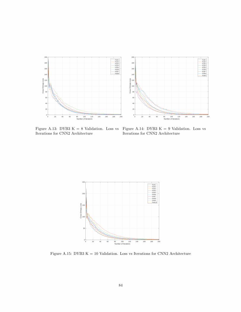
0 20 40 60 80 100 120 140 160 180 200
Number of Iterations
0
20
40
60
80
100
120
140
160
180
200
Cro
ss E
ntro
py L
oss
Fold 1Fold 2Fold 3Fold 4Fold 5Fold 6Fold 7Fold 8
Figure A.13: DYB3 K = 8 Validation. Loss vsIterations for CNN2 Architecture
0 20 40 60 80 100 120 140 160 180 200
Number of Iterations
0
20
40
60
80
100
120
140
160
180
200
Cro
ss E
ntro
py L
oss
Fold 1Fold 2Fold 3Fold 4Fold 5Fold 6Fold 7Fold 8Fold 9
Figure A.14: DYB3 K = 9 Validation. Loss vsIterations for CNN2 Architecture
0 20 40 60 80 100 120 140 160 180 200
Number of Iterations
0
50
100
150
200
250
Cro
ss E
ntro
py L
oss
Fold 1Fold 2Fold 3Fold 4Fold 5Fold 6Fold 7Fold 8Fold 9Fold 10
Figure A.15: DYB3 K = 10 Validation. Loss vs Iterations for CNN2 Architecture
84

A.2 Detection of Yellow-Boxes treated as a class extension to 4 class
Yellow-Box Classification
A.2.1 Results of CNN1 Architecture
This section includes plots of Loss vs Iterations for K-fold cross validation with K from 4
to 10, and one confusion matrix of classification performance for each K-fold cross validation.
85

Table A.15: DYB5 Confusion Matrix of K = 4Fold CNN1
51 5 7 2 10
5 10 5 3 2
2 3 11 5 2
0 2 1 16 0
2 1 1 2 16
Table A.16: DYB5 Confusion Matrix of K = 5Fold CNN1
38 8 9 2 9
0 12 1 1 0
2 2 8 1 2
1 1 1 11 5
5 1 1 0 10
Table A.17: DYB5 Confusion Matrix of K = 6Fold CNN1
30 1 4 0 1
0 14 6 1 0
1 0 3 1 2
4 1 4 14 0
3 0 0 0 20
Table A.18: DYB5 Confusion Matrix of K = 7Fold CNN1
32 2 5 1 1
2 5 0 1 0
4 3 6 1 0
0 0 0 11 0
4 0 0 2 14
Table A.19: DYB5 Confusion Matrix of K = 8Fold CNN1
23 3 2 1 5
2 13 0 0 0
1 3 4 0 4
1 1 0 8 0
1 0 0 0 10
Table A.20: DYB5 Confusion Matrix of K = 9Fold CNN1
20 2 5 1 2
2 5 2 0 0
1 1 4 0 0
2 0 1 10 0
2 0 1 1 11
Table A.21: DYB5 Confusion Matrix of K = 10 Fold CNN1
17 4 3 1 0
4 8 0 0 0
0 1 5 1 0
0 1 0 8 1
2 0 0 0 10
86
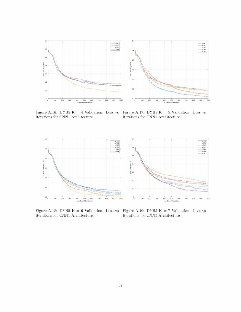
0 100 200 300 400 500 600 700 800 900 1000
Number of Iterations
1
1.1
1.2
1.3
1.4
1.5
1.6
1.7
Cro
ss E
ntro
py L
oss
Fold 1Fold 2Fold 3Fold 4
Figure A.16: DYB5 K = 4 Validation. Loss vsIterations for CNN1 Architecture
0 100 200 300 400 500 600 700 800 900 1000
Number of Iterations
1.1
1.2
1.3
1.4
1.5
1.6
1.7
Cro
ss E
ntro
py L
oss
Fold 1Fold 2Fold 3Fold 4Fold 5
Figure A.17: DYB5 K = 5 Validation. Loss vsIterations for CNN1 Architecture
0 100 200 300 400 500 600 700 800 900 1000
Number of Iterations
1.1
1.2
1.3
1.4
1.5
1.6
1.7
Cro
ss E
ntro
py L
oss
Fold 1Fold 2Fold 3Fold 4Fold 5Fold 6
Figure A.18: DYB5 K = 6 Validation. Loss vsIterations for CNN1 Architecture
0 100 200 300 400 500 600 700 800 900 1000
Number of Iterations
1
1.1
1.2
1.3
1.4
1.5
1.6
1.7
Cro
ss E
ntro
py L
oss
Fold 1Fold 2Fold 3Fold 4Fold 5Fold 6Fold 7
Figure A.19: DYB5 K = 7 Validation. Loss vsIterations for CNN1 Architecture
87
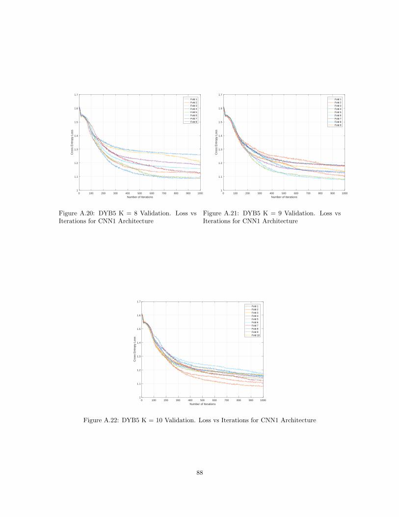
0 100 200 300 400 500 600 700 800 900 1000
Number of Iterations
1
1.1
1.2
1.3
1.4
1.5
1.6
1.7
Cro
ss E
ntro
py L
oss
Fold 1Fold 2Fold 3Fold 4Fold 5Fold 6Fold 7Fold 8
Figure A.20: DYB5 K = 8 Validation. Loss vsIterations for CNN1 Architecture
0 100 200 300 400 500 600 700 800 900 1000
Number of Iterations
1
1.1
1.2
1.3
1.4
1.5
1.6
1.7
Cro
ss E
ntro
py L
oss
Fold 1Fold 2Fold 3Fold 4Fold 5Fold 6Fold 7Fold 8Fold 9
Figure A.21: DYB5 K = 9 Validation. Loss vsIterations for CNN1 Architecture
0 100 200 300 400 500 600 700 800 900 1000
Number of Iterations
1
1.1
1.2
1.3
1.4
1.5
1.6
1.7
Cro
ss E
ntro
py L
oss
Fold 1Fold 2Fold 3Fold 4Fold 5Fold 6Fold 7Fold 8Fold 9Fold 10
Figure A.22: DYB5 K = 10 Validation. Loss vs Iterations for CNN1 Architecture
88

A.2.2 Results of CNN2 Architecture
This section includes plots of Loss vs Iterations for K-fold cross validation with K from 4
to 10, and one confusion matrix of classification performance for each K-fold cross validation.
Table A.22: DYB5 Confusion Matrix of K = 4Fold CNN2
57 0 8 0 1
3 23 3 0 0
5 2 9 0 0
1 0 2 26 1
2 1 2 0 18
Table A.23: DYB5 Confusion Matrix of K = 5Fold CNN2
42 0 5 0 0
2 23 1 1 0
5 1 10 0 3
0 0 0 20 2
0 0 0 0 16
Table A.24: DYB5 Confusion Matrix of K = 6Fold CNN2
40 0 3 0 1
4 13 2 0 0
1 0 12 0 0
0 0 1 18 0
3 1 1 0 10
Table A.25: DYB5 Confusion Matrix of K = 7Fold CNN2
25 0 5 0 0
1 19 2 0 0
0 1 7 0 0
0 0 2 16 0
2 1 0 0 13
Table A.26: DYB5 Confusion Matrix of K = 8Fold CNN2
28 0 4 0 0
1 10 3 0 0
2 1 6 0 1
1 0 1 15 1
0 0 0 0 8
Table A.27: DYB5 Confusion Matrix of K = 9Fold CNN2
17 0 2 0 0
1 12 4 0 0
3 1 6 0 1
0 0 0 12 1
0 0 0 0 13
Table A.28: DYB5 Confusion Matrix of K = 10 Fold CNN2
22 0 2 0 0
1 8 0 0 0
0 0 3 0 1
0 0 0 13 0
0 2 0 0 14
89

0 20 40 60 80 100 120 140 160 180 200
Number of Iterations
0
50
100
150
200
250C
ross
Ent
ropy
Los
sFold 1Fold 2Fold 3Fold 4
Figure A.23: DYB5 K = 4 Validation. Loss vsIterations for CNN2 Architecture
0 20 40 60 80 100 120 140 160 180 200
Number of Iterations
0
50
100
150
200
250
Cro
ss E
ntro
py L
oss
Fold 1Fold 2Fold 3Fold 4Fold 5
Figure A.24: DYB5 K = 5 Validation. Loss vsIterations for CNN2 Architecture
0 20 40 60 80 100 120 140 160 180 200
Number of Iterations
0
50
100
150
200
250
300
Cro
ss E
ntro
py L
oss
Fold 1Fold 2Fold 3Fold 4Fold 5Fold 6
Figure A.25: DYB5 K = 6 Validation. Loss vsIterations for CNN2 Architecture
0 20 40 60 80 100 120 140 160 180 200
Number of Iterations
0
50
100
150
200
250
Cro
ss E
ntro
py L
oss
Fold 1Fold 2Fold 3Fold 4Fold 5Fold 6Fold 7
Figure A.26: DYB5 K = 7 Validation. Loss vsIterations for CNN2 Architecture
90

0 20 40 60 80 100 120 140 160 180 200
Number of Iterations
0
50
100
150
200
250
Cro
ss E
ntro
py L
oss
Fold 1Fold 2Fold 3Fold 4Fold 5Fold 6Fold 7Fold 8
Figure A.27: DYB5 K = 8 Validation. Loss vsIterations for CNN2 Architecture
0 20 40 60 80 100 120 140 160 180 200
Number of Iterations
0
50
100
150
200
250
300
Cro
ss E
ntro
py L
oss
Fold 1Fold 2Fold 3Fold 4Fold 5Fold 6Fold 7Fold 8Fold 9
Figure A.28: DYB5 K = 9 Validation. Loss vsIterations for CNN2 Architecture
0 20 40 60 80 100 120 140 160 180 200
Number of Iterations
0
50
100
150
200
250
Cro
ss E
ntro
py L
oss
Fold 1Fold 2Fold 3Fold 4Fold 5Fold 6Fold 7Fold 8Fold 9Fold 10
Figure A.29: DYB5 K = 10 Validation. Loss vs Iterations for CNN2 Architecture
91
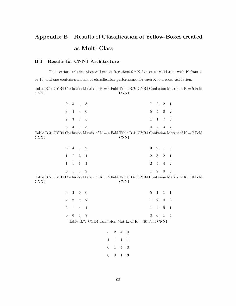
Appendix B Results of Classification of Yellow-Boxes treated
as Multi-Class
B.1 Results for CNN1 Architecture
This section includes plots of Loss vs Iterations for K-fold cross validation with K from 4
to 10, and one confusion matrix of classification performance for each K-fold cross validation.
Table B.1: CYB4 Confusion Matrix of K = 4 FoldCNN1
9 3 1 3
3 4 4 0
2 3 7 5
3 4 1 8
Table B.2: CYB4 Confusion Matrix of K = 5 FoldCNN1
7 2 2 1
5 5 0 2
1 1 7 3
0 2 3 7
Table B.3: CYB4 Confusion Matrix of K = 6 FoldCNN1
8 4 1 2
1 7 3 1
1 1 6 1
0 1 1 2
Table B.4: CYB4 Confusion Matrix of K = 7 FoldCNN1
3 2 1 0
2 3 2 1
2 4 4 2
1 2 0 6
Table B.5: CYB4 Confusion Matrix of K = 8 FoldCNN1
3 3 0 0
2 2 2 2
2 1 4 1
0 0 1 7
Table B.6: CYB4 Confusion Matrix of K = 9 FoldCNN1
5 1 1 1
1 2 0 0
1 4 5 1
0 0 1 4
Table B.7: CYB4 Confusion Matrix of K = 10 Fold CNN1
5 2 4 0
1 1 1 1
0 1 4 0
0 0 1 3
92

0 50 100 150 200 250 300 350 400 450 500
Number of Iterations
0.8
0.9
1
1.1
1.2
1.3
1.4
Cro
ss E
ntro
py L
oss
Fold 1Fold 2Fold 3Fold 4
Figure B.1: CYB4 K = 4 Validation. Loss vsIterations for CNN1 Architecture
0 50 100 150 200 250 300 350 400 450 500
Number of Iterations
0.8
0.9
1
1.1
1.2
1.3
1.4
Cro
ss E
ntro
py L
oss
Fold 1Fold 2Fold 3Fold 4Fold 5
Figure B.2: CYB4 K = 5 Validation. Loss vsIterations for CNN1 Architecture
0 50 100 150 200 250 300 350 400 450 500
Number of Iterations
0.8
0.9
1
1.1
1.2
1.3
1.4
Cro
ss E
ntro
py L
oss
Fold 1Fold 2Fold 3Fold 4Fold 5Fold 6
Figure B.3: CYB4 K = 6 Validation. Loss vsIterations for CNN1 Architecture
0 50 100 150 200 250 300 350 400 450 500
Number of Iterations
0.8
0.9
1
1.1
1.2
1.3
1.4
Cro
ss E
ntro
py L
oss
Fold 1Fold 2Fold 3Fold 4Fold 5Fold 6Fold 7
Figure B.4: CYB4 K = 7 Validation. Loss vsIterations for CNN1 Architecture
93

0 50 100 150 200 250 300 350 400 450 500
Number of Iterations
0.8
0.9
1
1.1
1.2
1.3
1.4
Cro
ss E
ntro
py L
oss
Fold 1Fold 2Fold 3Fold 4Fold 5Fold 6Fold 7Fold 8
Figure B.5: CYB4 K = 8 Validation. Loss vsIterations for CNN1 Architecture
0 50 100 150 200 250 300 350 400 450 500
Number of Iterations
0.8
0.9
1
1.1
1.2
1.3
1.4
Cro
ss E
ntro
py L
oss
Fold 1Fold 2Fold 3Fold 4Fold 5Fold 6Fold 7Fold 8Fold 9
Figure B.6: CYB4 K = 9 Validation. Loss vsIterations for CNN1 Architecture
0 50 100 150 200 250 300 350 400 450 500
Number of Iterations
0.8
0.9
1
1.1
1.2
1.3
1.4
Cro
ss E
ntro
py L
oss
Fold 1Fold 2Fold 3Fold 4Fold 5Fold 6Fold 7Fold 8Fold 9Fold 10
Figure B.7: CYB4 K = 10 Validation. Loss vs Iterations for CNN1 Architecture
94

B.1.1 Results of CNN2 Architecture
This section includes plots of Loss vs Iterations for K-fold cross validation with K from 4
to 10, and one confusion matrix of classification performance for each K-fold cross validation.
Table B.8: CYB4 Confusion Matrix of K = 4 FoldCNN2
13 3 1 1
3 18 3 3
0 1 12 3
0 2 0 9
Table B.9: CYB4 Confusion Matrix of K = 5 FoldCNN2
8 5 0 0
2 15 0 1
0 5 9 1
0 0 0 12
Table B.10: CYB4 Confusion Matrix of K = 6Fold CNN2
6 3 0 0
6 13 0 2
0 0 8 1
0 0 4 5
Table B.11: CYB4 Confusion Matrix of K = 7Fold CNN2
5 5 0 4
1 9 1 1
1 0 7 0
0 0 2 5
Table B.12: CYB4 Confusion Matrix of K = 8Fold CNN2
8 2 0 0
1 9 2 0
0 2 6 2
0 1 1 2
Table B.13: CYB4 Confusion Matrix of K = 9Fold CNN2
4 3 0 0
1 9 0 0
0 2 7 0
0 1 1 4
Table B.14: CYB4 Confusion Matrix of K = 10 Fold CNN2
4 1 1 0
1 1 0 2
0 1 7 2
0 0 0 4
95

0 20 40 60 80 100 120 140 160 180 200
Number of Iterations
0
50
100
150
200
250C
ross
Ent
ropy
Los
sFold 1Fold 2Fold 3Fold 4
Figure B.8: CYB4 K = 4 Validation. Loss vsIterations for CNN2 Architecture
0 20 40 60 80 100 120 140 160 180 200
Number of Iterations
0
50
100
150
200
250
Cro
ss E
ntro
py L
oss
Fold 1Fold 2Fold 3Fold 4Fold 5
Figure B.9: CYB4 K = 5 Validation. Loss vsIterations for CNN2 Architecture
0 20 40 60 80 100 120 140 160 180 200
Number of Iterations
0
50
100
150
200
250
300
Cro
ss E
ntro
py L
oss
Fold 1Fold 2Fold 3Fold 4Fold 5Fold 6
Figure B.10: CYB4 K = 6 Validation. Loss vsIterations for CNN2 Architecture
0 20 40 60 80 100 120 140 160 180 200
Number of Iterations
0
50
100
150
200
250
Cro
ss E
ntro
py L
oss
Fold 1Fold 2Fold 3Fold 4Fold 5Fold 6Fold 7
Figure B.11: CYB4 K = 7 Validation. Loss vsIterations for CNN2 Architecture
96
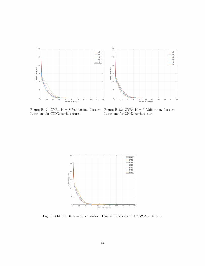
0 20 40 60 80 100 120 140 160 180 200
Number of Iterations
0
50
100
150
200
250
300
Cro
ss E
ntro
py L
oss
Fold 1Fold 2Fold 3Fold 4Fold 5Fold 6Fold 7Fold 8
Figure B.12: CYB4 K = 8 Validation. Loss vsIterations for CNN2 Architecture
0 20 40 60 80 100 120 140 160 180 200
Number of Iterations
0
50
100
150
200
250
300
Cro
ss E
ntro
py L
oss
Fold 1Fold 2Fold 3Fold 4Fold 5Fold 6Fold 7Fold 8Fold 9
Figure B.13: CYB4 K = 9 Validation. Loss vsIterations for CNN2 Architecture
0 20 40 60 80 100 120 140 160 180 200
Number of Iterations
0
50
100
150
200
250
300
Cro
ss E
ntro
py L
oss
Fold 1Fold 2Fold 3Fold 4Fold 5Fold 6Fold 7Fold 8Fold 9Fold 10
Figure B.14: CYB4 K = 10 Validation. Loss vs Iterations for CNN2 Architecture
97

Bibliography
[1] I Arel, D C Rose, and T P Karnowski. Deep machine learning - a new frontier in artificialintelligence research [research frontier]. IEEE Computational Intelligence Magazine, 5(4):13–18, 2010.
[2] K. S. Bagalore. Studying the use of hidden markov models in the detection and classificationof eeg epileptiform tranients using lpc features. Clemson University, All Theses. 2569., 2016.
[3] A. Botev, G. Lever, and D. Barber. Nesterov’s Accelerated Gradient and Momentum as ap-proximations to Regularised Update Descent. ArXiv e-prints, July 2016.
[4] Yann Le Cun, Leon Bottou, and Yoshua Bengio. Reading checks with multilayer graph trans-former networks. Speech and Image Processing Services Research Lab, AT&T Labs, 1998.
[5] John Duchi, Elad Hazan, and Yoram Singer. Adaptive subgradient methods for online learningand stochastic optimization. Journal of Machine Learning Research, 12(Jul):2121–2159, 2011.
[6] V. Dumoulin and F. Visin. A guide to convolution arithmetic for deep learning. ArXiv e-prints,2016.
[7] Robert S. Fisher, Carlos Acevedo, Alexis Arzimanoglou, Alicia Bogacz, J. Helen Cross, Chris-tian E. Elger, Jerome Engel, Lars Forsgren, Jacqueline A. French, and Mike et al. Glynn. Ilaeofficial report: A practical clinical definition of epilepsy. Epilepsia, 55(4):475–482, 2014.
[8] J.R. Glover, N. Raghaven, P.Y. Ktonas, and J.D. Frost. Context-based automated detection ofepileptogenic sharp transients in the eeg: elimination of false positives. IEEE Transactions onBiomedical Engineering, 36(5):519–527, 1989.
[9] Jonathan J. Halford, Robert J. Schalkoff, Jing Zhou, Selim R. Benbadis, William O. Tatum,Robert P. Turner, Saurabh R. Sinha, Nathan B. Fountain, Amir Arain, and Paul B. et al.Pritchard. Standardized database development for eeg epileptiform transient detection: Eegnetscoring system and machine learning analysis. Journal of Neuroscience Methods, 212(2):308–316, 2013.
[10] Jasper Herbert H. Report of the committee on methods of clinical examination in electroenchep-alography. Electroencephalography and Clinical Neurophysiology, 10(2):370–375, 1958.
[11] Sergey Ioffe and Christian Szegedy. Batch normalization: Accelerating deep network trainingby reducing internal covariate shift. CoRR, abs/1502.03167, 2015.
[12] R. Jagadeesha. Detection and classification of eeg epileptiform transients with rbf networksusing hilbert huang transform-derived features. Clemson University, All Theses., 2016.
[13] Yosuke Kakisaka, Andreas V. Alexopoulos, Ajay Gupta, Zhong I. Wang, John C. Mosher,Masaki Iwasaki, and Richard C. Burgess. Generalized 3-hz spike-and-wave complexes emanatingfrom focal epileptic activity in pediatric patients. Epilepsy and Behavior, 20(1):103–106, 2011.
98

[14] D. P. Kingma and J. Ba. Adam: A Method for Stochastic Optimization. ArXiv e-prints,December 2014.
[15] Timo Kirschstein and Rdiger Khling. What is the source of the eeg? Clinical EEG andNeuroscience, 40(3):146–149, 2009.
[16] Alex Krizhevsky, Ilya Sutskever, and Geoffrey E Hinton. Imagenet classification with deepconvolutional neural networks. Advances in Neural Information Processing Systems 25, pages1097–1105, 2012.
[17] Y. Lecun, L. Bottou, Y. Bengio, and P. Haffner. Gradient-based learning applied to documentrecognition. Proceedings of the IEEE, 86(11):2278–2324, 1998.
[18] Tianyi Liu, Shuangsang Fang, Yuehui Zhao, Peng Wang, and Jun Zhang. Implementationof training convolutinal neural networks. University of Chinese Academy of Sciences. BeijingChina.
[19] Jonathan Long, Evan Shelhamer, and Trevor Darrell. Fully convolutional networks for se-mantic segmentation. Proceedings of the IEEE Conference on Computer Vision and PatternRecognition, pages 3431–3440, 2015.
[20] Pankaj Malhotra, Lovekesh Vig, Gautam Shroff, and Puneet Agarwal. Long short term memorynetworks for anomaly detection in time series. In Proceedings, page 89. Presses universitairesde Louvain, 2015.
[21] Tania Morimoto and Sean Sketch. Classifying brain’s motor activity via deep learning. StanfordUniversity, CS 229 Machine Learning., 2014.
[22] Ewan Nurse, Benjamin S. Mashford, Antonio Jimeno Yepes, Isabell Kiral-Kornek, Stefan Har-rer, and Dean R. Freestone. Decoding eeg and lfp signals using deep learning. CF ’16 Proceedingsof the ACM International Conference on Computing Frontiers, pages 259–266, 2016.
[23] U Orhan, D Erdogmus, KE Hild, B Roark, B Oken, and M Fried-Oken. Context informationsignificantly improves brain computer interface performance - a case study on text entry using alanguage model assisted bci. Asilomar Conference on Signals, Systems and Computers AsilomarConference on Signals, Systems and Computers, 45:132–136, 2011.
[24] E. Parvinnia, M. Sabeti, M. Zolghadri Jahromi, and R. Boostani. Classification of eeg signalsusing adaptive weighted distance nearest neighbor algorithm. Journal of King Saud University- Computer and Information Sciences, 26(1):1–6, 2014.
[25] S. Rajendran. Identification and use of psd-derived features for the contextual detection andclassification of eeg epileptiform transients. Clemson University, All Theses. 2442., 2016.
[26] Robert J Schalkoff. Artificial neural networks. McGraw-Hill, 1 edition, 1997.
[27] L. Senhadji, J. L. Dillenseger, F. Wendling, C. Rocha, and A. Kinie. Wavelet analysis of eeg forthree-dimensional mapping of epileptic events. Annals of Biomedical Engineering, 23(5):543–552, 1995.
[28] Wenzhe Shi, Jose Caballero, Lucas Theis, Ferenc Huszar, Andrew P. Aitken, Christian Ledig,and Zehan Wang. Is the deconvolution layer the same as a convolutional layer? CoRR,abs/1609.07009, 2016.
[29] Benbadis SR. Errors in eegs and the misdiagnosis of epilepsy: importance, causes, consequences,and proposed remedies. Epilepsy Behav, 11:257–62, 2007.
99
[30] Vairavan Srinivasan, Chikkannan Eswaran, and Natarajan Sriraam. Approximate entropy-basedepileptic eeg detection using artificial neural networks. IEEE Transactions on InformationTechnology in Biomedicine, 11(3):288–295, 2007.
[31] Nitish Srivastava, Geoffrey E Hinton, Alex Krizhevsky, Ilya Sutskever, and Ruslan Salakhutdi-nov. Dropout: a simple way to prevent neural networks from overfitting. Journal of MachineLearning Research, 15(1):1929–1958, 2014.
[32] Ian Walker. Deep convolutional neural networks for brain computer interface using motorimagery. Thesis, Department of Computing, Imperial College London., 2015.
[33] Jianxin Wu. Introduction to convolutional neural networks. National Key Lab for Novel Soft-ware Technology. Nanjing University. China, 2017.
[34] D F Wulsin, J R Gupta, R Mani, J A Blanco, and B Litt. Modeling electroencephalographywaveforms with semi-supervised deep belief nets: fast classification and anomaly measurement.Journal of Neural Engineering, 8(3):036015, 2011.
[35] M. D. Zeiler. ADADELTA: An Adaptive Learning Rate Method. ArXiv e-prints, December2012.
[36] Matthew D Zeiler and Rob Fergus. Visualizing and understanding convolutional networks.European conference on computer vision, pages 818–833, 2014.
[37] Tong Zhang. Statistical behavior and consistency of classification methods based on convex riskminimization. Annals of Statistics, pages 56–85, 2004.
[38] Jing Zhou, R. J. Schalkoff, B. C. Dean, and J. J. Halford. Morphology-based wavelet fea-tures and multiple mother wavelet strategy for spike classification in eeg signals. 2012 AnnualInternational Conference of the IEEE Engineering in Medicine and Biology Society, 2012.
100


