Download - Differential Geometry A Short Summary - polito.it · Diﬀerential Geometry A Short Summary Basilio Bona ... Diﬀerential geometry is closely related with ... bracket as the operator

Differential Geometry

A Short Summary

Basilio Bona

DAUIN – Politecnico di Torino

July 2009

Geometric and Probabilistic Fundamentals in Robotics

B. Bona (DAUIN) Differential geometry July 2009 1 / 24

Introduction

Differential geometry is a mathematical discipline that uses the methods ofdifferential and integral calculus to study problems in geometry.

The theory of plane and space curves and of surfaces in thethree-dimensional Euclidean space formed the basis for its initialdevelopment in the eighteenth and nineteenth century.

Since the late nineteenth century, differential geometry has grown into afield concerned more generally with geometric structures on differentiablemanifolds.

Differential geometry is closely related with differential topology and withthe geometric aspects of the theory of differential equations.

Basic concepts of differential geometry are required to study the behaviourof mechanical systems subject to nonholonomic constraints, such aswheeled mobile robots and free flying bodies subject to angular momentconservation.


Differentiable manifolds

A differentiable manifold is a space that is locally diffeomorphic to Rn.

Figure: A differential manifold.


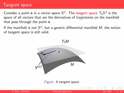
Tangent space

Consider a point x in a vector space Rn. The tangent space TxR

n is thespace of all vectors that are the derivatives of trajectories on the manifoldthat pass through the point x.

If the manifold is not Rn, but a generic differential manifold M, the notion

of tangent space is still valid.

Figure: A tangent space.


Vector fields

A vector field f : Rn 7→ TxR

n is a smooth mapping that assigns to eachpoint x a tangent vector f(x) in the tangent space

x → f(x)

Smooth means that the mapping is differentiable up to what is necessary.

Figure: A vector field.


In other words, a vector field assigns a tangent vector to each point x inthe manifold, in an appropriately smooth way (notice the differencebetween point and vector).

Vector fields can be studied as differential operators and can be used todifferentiate functions and other vector fields.

There is one-to-one correspondence between ordinary differential equationsand vector fields.

Vector fields are to be thought as right-hand sides of differential equations

x = f(x)

Of great importance is the Lie bracket operator between vector fields: it isdefined as an appropriate composition of differential operators, and itfrequently arises in the composition of flows of differential equations.


Flows

A flow of f is defined when a vector field f(x) is used to specify adifferential equation

x(t) = f(x(t))

The flow φft(x) is then the mapping that associates to each point x the

value at time t of the solution of the above differential equation, evolvingfrom x(t) at t = 0, or

d

dtφf

t(x) = f(φft(x))

For time-invariant linear systems, the differential equation takes the form

x(t) = Ax(t)

and the flow becomes the well know linear operator

φft(x) = eAtx hence φf

t = eAt


Lie bracket

Given two vector fields g and h the composition of their flow is in generalnon commutative

φgt φh

t 6= φht φ

gt

A Lie bracket [g,h] can be defined using the vector fields as

[g,h] =∂h

∂xg −

∂g

∂xh = Jhg − Jgh

Properties:

[f,g] = −[g, f]

[f, [g,h]] + [g, [h, f]] + [h, [f,g]] = 0

if [f,g] = 0, the two vector fields commute.

f always commute with itself: [f, f] = 0


Lie algebra

A vector space V over R is a Lie algebra, if there exists a binary operationV × V → V, denoted [·, ·], that a) is skew-symmetric, and b) satisfy theJacobi identity.

The vector space of smooth vector fields on Rn, equipped with the Lie

bracket as the operator between space elements, is a Lie algebra, denotedby X(Rn).


Lie derivative

A Lie derivative Lfg evaluates the change of one vector field g along theflow of another vector field f.

The Lie derivatives are represented by vector fields, as infinitesimalgenerators of flows (active diffeomorphisms) on a manifold M. Looking atit the other way around, the diffeomorphism group of M has theassociated Lie algebra structure, of Lie derivatives, in a way directlyanalogous to the Lie group theory.

In our case the manifold M is the (flat) Euclidean space Rn.


Given two vector fields f,g : D 7→ Rn the Lie derivative is

Lfg(x) =∂g

∂xf

hence[f,g] = Lfg(x) − Lgf(x)

When the vector field f is a real valued function f (x) : Rn 7→ R, the Lie

derivative is

Lgf (x) =∂f

∂xg(x)

A Lie product is a nested set of Lie brackets, as, for example, in

[[f,g], [f , [f,g]]]


Given two real valued functions f1(x) and f2(x), the following holds

Lg(f1f2) = (Lgf1)f2 + (Lgf2)f1

Given two real valued functions f1(x) and f2(x) and two vector fields g,h,the following holds

[f1g, f2h] = f1f2[g,h] + f1(Lgf2)h − f2(Lhf1)g

Another characterization of Lie brackets

L[g,h]f = LgLhf − LhLgf


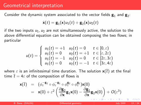
Geometrical interpretation

Consider the dynamic system associated to the vector fields g1 and g2:

x(t) = g1(x)u1(t) + g2(x)u2(t)

if the two inputs u1, u2 are not simultaneously active, the solution to theabove differential equation can be obtained composing the two flows; inparticular

u(t) =

u1(t) = +1 u2(t) = 0 t ∈ [0, ε)u1(t) = 0 u2(t) = +1 t ∈ [ε, 2ε)u1(t) = −1 u2(t) = 0 t ∈ [2ε, 3ε)u1(t) = 0 u2(t) = −1 t ∈ [3ε, 4ε)

where ε is an infinitesimal time duration. The solution x(t) at the finaltime t = 4ε of the composition of flows is

x(t) = (φ−g2ε φ

−g1ε φ

g2ε φ

g1ε )x(0)

= x(0) + ε2

(∂g2

∂xg1x(0) −

∂g1

∂xg2x(0)

)

+ O(ε3)


Hence, neglecting the higher order infinitesimal,

x(t) − x(0) = [g1,g2]x(0)

Figure: A Lie bracket motion.


An important conclusion derived from the previous analysis is that thesystem can achieve infinitesimal motions not only along the two field f,g,but also along the infinitesimal direction specified by the Lie bracket [f,g].

More complicated motions are possible along higher order Lie brackets,such as [f, [f,g]].

Usually the following notations are used

ad0f g = g

adfg = [f,g]

adk

f g = [f, adk−1f g], k ≥ 1


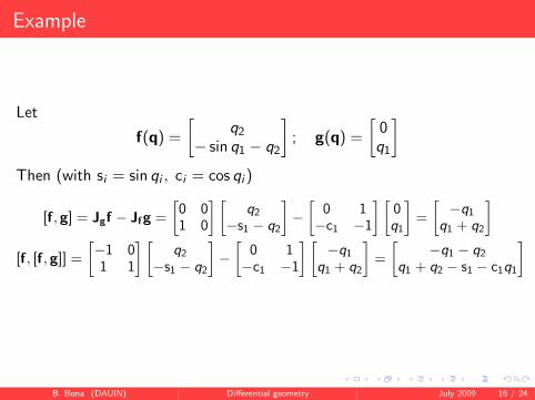
Example

Let

f(q) =

[q2

− sin q1 − q2

]

; g(q) =

[0q1

]

Then (with si = sin qi , ci = cos qi )

[f, g] = Jgf − Jfg =

[0 01 0

] [q2

−s1 − q2

]

−

[0 1

−c1 −1

] [0q1

]

=

[−q1

q1 + q2

]

[f, [f, g]] =

[−1 01 1

] [q2

−s1 − q2

]

−

[0 1

−c1 −1

] [−q1

q1 + q2

]

=

[−q1 − q2

q1 + q2 − s1 − c1q1

]


Dynamic systems

The dynamic system

x(t) = g1(x)u1(t) + g2(x)u2(t)

is said to be a driftless system, since, as long as the control inputs remainzero, the state does not vary.

A system described by a drift vector field is, for example, the following

x(t) = f(x) + g1(x)u1(t) + g2(x)u2(t)


Example

Assuming the SISO linear time-invariant dynamical system, given by thefollowing matrix differential equation

x(t) = Ax(t) + bu(t)

where f(x) = Ax is the drift vector field, and g(x) = b is the input vectorfield, we can compute the various Lie brackets

[f,g] =∂g

∂xf −

∂f

∂xg =

∂b

∂xAx

︸︷︷︸

0

−∂Ax

∂xb

︸︷︷︸

Ab

= −Ab = −[g, f]

[f, [f,g]] = [Ax,−Ab] =∂(−Ab)

∂xAx

︸︷︷︸

0

+∂Ax

∂xAb

︸︷︷︸

A2b

= A2b

[f, [f, [f,g]]] = −A3b etc.

that corresponds to the columns of the controllability matrix, i.e., thedirections along which it is possible to move the system.


Distributions

It is convenient to think about a vector field f as a vector in Rn

f(x) =[f1(x) · · · fn(x)

]T

If α(x) is a smooth function Rn 7→ R, then α(x)f(x) is also a vector field

and the sum of two vectors field is also a vector field. Thus the vector fieldis a module over the ring of smooth functions defined on U ∈ R

n, denotedby C∞(U).

A module is a linear space for which the “scalars” are elements of a ring.Also, the space of vector fields is a vector space over the field of reals.

Now we have this definition: given a set of smooth vector fieldsf1(x), . . . , fm(x), we define the distribution ∆(x) to be

∆(x) = span f1(x), · · · , fm(x)

i.e., the elements of ∆ at the point x are of the form

α1(x)f1(x) + α2(x)f2(x) + · · · + αm(x)fm(x)


Distributions and rank

Some remarks:

1 A distribution is a smooth assignment of a subspace of Rn to each

point x

2 If F ∈ Rm×n is the matrix obtained by stacking the f i (x) next to each

other, then∆(x) = Image F

We may now define the rank of the distribution at x as the rank of F(x);this rank, denoted by ρF(x) is not, in general, a constant function of x.

If the rank is locally (i.e., in a neighborhood of x) constant, the x is saidto be a regular point of the distribution.

If every point is regular, the distribution is said to be regular, i.e.,nonsingular.


Involutive distributions

A distribution ∆(x) is called involutive if for any two vector fields in thedistribution f1, f2 ∈ ∆(x), their Lie bracket [f1, f2] ∈ ∆(x) is also in thedistribution.

Any one-dimensional distribution f (x) (associated with a singlevector field) is involutive, since if ∆ = spanf (x), then

[α1(x)f (x), α2(x)f (x)] ∈ spanf (x)

for any α1(x), α2(x) ∈ C∞.

A basis set is said to commute if [f1, f2] = 0. A distribution with acommutative basis set is involutive.

The involutive closure ∆ of a distribution ∆ is its closure under the Liebracket operation.

Hence, ∆ is involutive iff it coincides with its closure ∆ = ∆.

The distribution of a single vector field f is always involutive.


Example

Assuming the two vector fields

g1 =[c3 s3 0

]T, g2 =

[0 0 1

]T

The associated distribution

∆ = spang1(x),g2(x)

is nonsingular and has dimension 2. Now, if we compute the Lie bracket

[g1,g2] =[s3 −c3 0

]T

we notice that ∆ is not involutive, since the Lie bracket is alwaysindependent of g1,g2..

The involutive closure ∆ is therefore

∆ = spang1,g2, [g1,g2]


The dual of a distribution is a codistribution (remember the definition ofdual spaces; moreover,elements of codistributions are row vectors).

A distribution Ω is said to annihilate or be perpendicular to a distribution∆ if for every ω ∈ Ω, f ∈ ∆

ω · f = 0

In the previous example, the distribution

Ω = span[g1,g2]

was perpendicular to ∆.


References

[01] F. Bullo, A.D. Lewis, Geometric Control of Mechanical Systems,Springer, 2005.

[02] H.K. Khalil, Nonlinear Systems, III Ed. Springer, 2002.

[03] Z. Qu, Cooperative Control of Dynamical Systems: Applications to

Autonomous Vehicles, Springe, 2009

[04] S. Sastry, Nonlinear Systems: Analysis, Stability, and Control,Springer, 1999.

[05] B. Siciliano, L. Sciavicco, L. Villani, G. Oriolo, Robotics: Modelling,

Planning and Control, Springer, 2009.


Download - Differential Geometry A Short Summary - polito.it · Diﬀerential Geometry A Short Summary Basilio Bona ... Diﬀerential geometry is closely related with ... bracket as the operator

Top Related