Download - Digital Twin Workshop Harry Millwater University of Texas at San Antonio Sept. 10-11, 2012 1

Digital Twin Digital Twin WorkshopWorkshop
Harry MillwaterHarry Millwater
University of Texas at San AntonioUniversity of Texas at San Antonio
Sept. 10-11, 2012Sept. 10-11, 2012
1
TopicsTopics
FAA Probabilistic Damage FAA Probabilistic Damage Tolerance AnalysisTolerance Analysis
System Reliability AnalysisSystem Reliability Analysis Sensitivity MethodsSensitivity Methods
2

Damage Tolerance Damage Tolerance MethodologyMethodology
Geometry
…54
321
n
Sensitivities
Insp 1
Insp 2
Time
RS
EIFS
Insp 1
Insp 2
Time
Crack Size
Loading EVD POD
SFPOF & CTPOF
Material Prop.

POF CalculationsPOF Calculations
4
€
SFPOF(T) = FEVD
KC
β(ao, t) πa(ao, t)
⎛
⎝ ⎜ ⎜
⎞
⎠ ⎟ ⎟
t =1
T −1
∏ ⎡
⎣ ⎢ ⎢
⎤
⎦ ⎥ ⎥1 − FEVD
KC
β(ao,T) πa(ao,T)
⎛
⎝ ⎜ ⎜
⎞
⎠ ⎟ ⎟
⎡
⎣ ⎢ ⎢
⎤
⎦ ⎥ ⎥fa0
(a0) fKc(Kc )da0dKc
0
∞
∫−∞
∞
∫
Survival t-1 POF Flight t
€
CTPOF(t) =1
N1 − (1 − SFPOF(t))
t =1
T
∏ ⎡
⎣ ⎢
⎤
⎦ ⎥
i=1
N
∑
R(t) =1 − CTPOF(t)
hz(t) =1
R(t)SFPOF(t)

EVD ResultsEVD Results
5
Flight 1 Flight 2
...Flight n
FrechetGumbelWeibull

EVD ResultsEVD Results
6
Usage Location Scale Shape DistributionSingle Engine Unpress. Basic
Inst.14.49 1.75 0.01 Frechet
Single Engine Unpress. Personal
12.03 1.15 0.00 Gumbel
Single Engine Unpress. Executive
11.68 0.90 -0.04 Weibull
Twin Engine Unpress. Basic Inst.
13.93 1.42 0.00 Gumbel
Twin Engine Unpress. General
12.05 1.16 0.02 Frechet
Pressurized 13.41 1.26 0.02 FrechetAgric/Special 12.07 0.94 -0.12 Weibull
Special Usage Survey 14.56 1.32 -0.05 Weibull

7
POF contours
Probabilistic Probabilistic Modeling of SystemsModeling of Systems
L. Domyancic, D. Sparkman, and H.R. Millwater, L. Smith and D. Wieland, “A Fast First-Order Method for Filtering Limit States,” 50 th AIAA AIAA Nondeterministic Approaches Conference, May 4-7, 2009, Palm Springs, CA, AIAA 2009-2260

Pair-wise Filtering Pair-wise Filtering CriteriaCriteria
Pair-wise filtering – neglect limit states Pair-wise filtering – neglect limit states that don’t contribute significantly to the that don’t contribute significantly to the system POF system POF relative to relative to the dominant limit the dominant limit statesstates
8
€
γi =P g1 giU[ ] − P g1[ ]
P g1[ ]i = 2,n
g1 – dominant limit state, serves as a benchmark
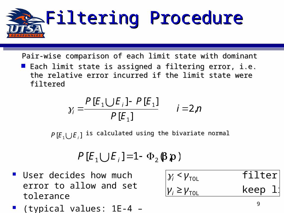
Filtering ProcedureFiltering Procedure
Pair-wise comparison of each limit state with dominantPair-wise comparison of each limit state with dominant Each limit state is assigned a filtering error, i.e. the Each limit state is assigned a filtering error, i.e. the
relative error incurred if the limit state were filteredrelative error incurred if the limit state were filtered
γi P[E1 E i ] P[E1]
P[E1] i 2,n
9
is calculated using the bivariate normalis calculated using the bivariate normal
P[E1 E i ]1 2(;)
P[E1 E i ]
User decides how much error to allow and set tolerance
(typical values: 1E-4 – 1E-6)
€
γi < γ TOL filter limit state
γ i ≥ γ TOL keep limit state

Second Order BoundsSecond Order Bounds
Examine the cumulative effect of the filtered Examine the cumulative effect of the filtered limit states using 2limit states using 2ndnd order bounds order bounds
Compare bounds from a) all limit states vs. b) only Compare bounds from a) all limit states vs. b) only unfiltered limit statesunfiltered limit states
10
P1 max Pi Pij ;0j1
i 1
i2
m
Pfs Pi
i1
m
maxji
Piji2
m

Aircraft ModelAircraft Model
Lower wing skin analyzed, ~900 limit statesLower wing skin analyzed, ~900 limit states
Root radius Element 292 and 277 left unfiltered (Root radius Element 292 and 277 left unfiltered (γγTOLTOL =1E- =1E-6)6)
Bounds on entire system vs. only critical locations widen Bounds on entire system vs. only critical locations widen by 1E-5by 1E-5
11
g1
LS # Beta Corr. Filt. Error292 0.297 1 0277 0.65 0.99 2.50E-04256 0.949 0.98 2.20E-09

Sensitivity MethodsSensitivity Methods
Numerical Differentiation (*)Numerical Differentiation (*) VisualVisual Linear RegressionLinear Regression Score Function partial derivativesScore Function partial derivatives Local probabilistic partial derivatives Local probabilistic partial derivatives
(*)(*) Global Sensitivity AnalysisGlobal Sensitivity Analysis

Local Prob. Sensitivity
Original CDFModified CDF

ZFEM Complex ZFEM Complex Variable FE MethodVariable FE Method
€
P
0
⎧ ⎨ ⎩
⎫ ⎬ ⎭=
EI
L3
12 6L
6L 4L2
⎡
⎣ ⎢
⎤
⎦ ⎥δ
φ
⎧ ⎨ ⎩
⎫ ⎬ ⎭
€
P
0
⎧ ⎨ ⎩
⎫ ⎬ ⎭=
EI
(L + ih)3
12 6(L + ih)
6(L + ih) 4(L + ih)2
⎡
⎣ ⎢
⎤
⎦ ⎥δ
φ
⎧ ⎨ ⎩
⎫ ⎬ ⎭
€
δ =PL3
3EI−
PLh2
EI
⎧ ⎨ ⎩
⎫ ⎬ ⎭+ i
PL2h
EI−
Ph3
3EI
⎧ ⎨ ⎩
⎫ ⎬ ⎭
€
∂δ∂L
= Im[δ ]/h

Abaqus 2D Verification
Analytical Abaqus
€
∂σθ
∂ri

Strain Energy Release Rate
Double Cantilever Beam (DBC)
Exact = 0.800
Exact = 0.8
€
G = −∂U
∂a
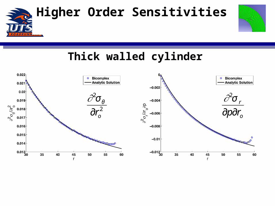
Higher Order Sensitivities
€
∂2σ θ
∂ro2
€
∂2σ r
∂p∂ro
Thick walled cylinder


