
div grad an
informal text
and on vector calculus
that
fourth edition
h. m. schev

DIVERGENCE THEOREM
F • n dS = • F dV
STOKES’ THEOREM
F • t ds V X F dS
IDENTITIES INVOLVING THE OPERATOR V*
V(/g)=/Vg + gV/
V(F • G) = (G • V)F + (F • V)G + FX(VxG) + Gx(VxF)
V • (/F) =/V • + F • V/
V • (F X G) = G • (V X F) - F • (V X G)
V* V X F = 0
V X (/F) =/V x F + (V/) X F
V x (F x G) = (G • V)F - (F • V)G + F(V • G) - G(V • F) V X (V x F) = V(V • F) - V2F
V X V/ = 0
/and g are scalar functions of position, and F and G are vector functions of position.

div, grad, curl, and all that
fourth edition
BUSINESS/SC lE NC E/TECHNOLOGY DIVISION
CHICAGO PUBLIC LIBRARY
400 SOUTH STATE STREET
CHICAGO, IL 60605

div, grad,
an informal text

h. m. schey
curl, and all that
on vector calculus
fourth edition
W • W • NORTON & COMPANY
New York • London

W.W. Norton & Company has been independent since its founding in 1923, when William Warder
Norton and Mary D. Herter Norton first published lectures delivered at the People’s Institute, the
adult education division of New York City’s Cooper Union. The Nortons soon expanded their
program beyond the Institute, publishing books by celebrated academics from America and
abroad. By mid-century, the two major pillars of Norton’s publishing program—trade books and
college texts—were firmly established. In the 1950s, the Norton family transferred control of the
company to its employees, and today—with a staff of four hundred and a comparable number of
trade, college, and professional titles published each year—W.W. Norton & Company stands as
the largest and oldest publishing house owned wholly by its employees.
Copyright © 2005, 1997, 1992, 1973 by W.W. Norton &
Company, Inc.
All rights reserved
Printed in the United States of America
Composition by GGS Book Services, Atlantic Highlands
Library of Congress Cataloging-in-Publication Data
Schey, H. M. (Harry Moritz), 1930-
Div, grad, curl, and all that: an informal text on vector
calculus / H.M. Schey.—4th ed.
p. cm.
Includes index.
1. Vector analysis. I. Title.
QA433.S28 2004
515'.63—dc22
2004053199
ISBN 0-393-92516-1 (pbk.)
W. W. Norton & Company, Inc., 500 Fifth Avenue, New York, N.Y. 10110
www.wwnorton.com
W. W. Norton & Company Ltd., Castle House, 75/76 Wells Street, London WIT 3QT
34567890

Rosom mma3a
SUSiNESS/SClENCE/TECHfif •
CHICAGO PUBLIC iifiMAhr 4m SOUTH STATE STREET
©WCAQQ, SL SOSOS
Zusammengestohlen aus Verschiedenem diesem und jenem.
v-.c.UM
Ludwig van Beethoven

Contents
Preface to the Fourth Edition ix
Chapter I Introduction, Vector Functions, and Electrostatics 1
Introduction 1
Vector Functions 2
Electrostatics 5
Problems 8
Chapter II Surface Integrals and the Divergence 11
Gauss’ Law 11
The Unit Normal Vector 12
Definition of Surface Integrals 17
Evaluating Surface Integrals 21
Flux 31
Using Gauss’ Law to Find the Field 33
The Divergence 37
The Divergence in Cylindrical and Spherical
Coordinates 42
The Del Notation 44
The Divergence Theorem 45
Two Simple Applications of the Divergence
Theorem 49
Problems 52

Contents Chapter III Line Integrals and the Curl 63
Work and Line Integrals 63
Line Integrals Involving Vector Functions 66
Path Independence 71
The Curl 75
The Curl in Cylindrical and Spherical Coordinates 82
The Meaning of the Curl 86
Differential Form of the Circulation Law 91
Stokes’ Theorem * 93
An Application of Stokes’ Theorem 99
Stokes’ Theorem and Simply Connected Regions 101
Path Independence and the Curl 103
Problems 104
Chapter IV The Gradient 115
Line Integrals and the Gradient 115
Finding the Electrostatic Field 121
Using Laplace’s Equation 124
Directional Derivatives and the Gradient 131
Geometric Significance of the Gradient 137
The Gradient in Cylindrical and Spherical
Coordinates 141
Problems 144
Solutions to Problems 156
Index 161
viii
Preface to the Fourth Edition
Can we ever have too much of a good thing?
Miguel de Cervantes
This new edition differs from the Third in two major respects.
First, a number of new worked examples have been added. This
has been done in response to the comments of many students that
such examples would be an aid in understanding the material and
useful in preparing them to do the problem sets. My task was to
add enough examples to be helpful, without at the same time
lengthening the text significantly. (Two reviewers urged me not to
lengthen the book at all, inadvertently providing an answer to
Sr. de Cervantes’ question.)
The second major difference between this edition and its prede¬
cessor involves switching the roles of the two spherical angles 0
and c|>. Years ago, when the book was written it was common to
use 0 as the polar angle and <j> as the azimuthal. Nowadays, the
more common convention reverses this, making 0 the azimuthal
angle and 4> the polar, the convention we adopt in this edition.
I wish to thank the many readers who, over the years, have
written me with suggestions for improvements in the text. These
suggestions have often been adopted and have been an important
reason for the book’s very long lifetime.

Chapter I
Introduction, Vector Functions, and Electrostatics
One lesson, Nature, let me learn of thee.
Matthew Arnold
Introduction
In this text the subject of vector calculus is presented in the con¬
text of simple electrostatics. We follow this procedure for two
reasons. First, much of vector calculus was invented for use in
electromagnetic theory and is ideally suited to it. This presenta¬
tion will therefore show what vector calculus is and at the same
time give you an idea of what it’s for. Second, we have a deep-
seated conviction that mathematics—-in any case some mathe¬
matics—is best discussed in a context that is not exclusively
mathematical. Thus, we will soft-pedal mathematical rigor. 1

Introduction, which we think is an obstacle to learning this subject on a first
Vector Functions, exposure to it, and appeal as much as possible to physical and
and Electrostatics geometric intuition.
Now, if you want to learn vector calculus but know little or
nothing about electrostatics, you needn’t be put off by our ap¬
proach; no very great knowledge of physics is required to read
and understand this text. Only the simplest features of electrostat¬
ics are involved, and these are presented in a few pages near the
beginning. It should not be an impediment to anyone. In fact, the
entire discussion is based on a search for a convenient method of
finding the electrostatic field given the distribution of electric
charges which produce it. This is the thread that runs through, and
unifies, our presentation, so that as a bare minimum all you really
need do is take our word for the fact that the electric field is an
important enough quantity to warrant spending some time and ef¬
fort in setting up a general method for calculating it. In the
process, we hope you will learn the elements of vector calculus.
Having said what you do not need to know, we must now say
what you do need to know. To begin with, you should, of course,
be fluent in elementary calculus. Beyond that you should know
how to work with functions of several variables, partial deriva¬
tives, and multiple (double and triple) integrals.1 Finally, you
must know something about vectors. This, however, is a subject
of which too many writers and teachers have made heavy
weather. What you should know about it can be listed quickly:
definition of vector, addition and subtraction of vectors, multipli¬
cation of vectors by scalars, dot and cross products, and finally,
resolution of vectors into components. An hour’s time with any
reasonable text on the subject should provide you with all you
need to know of it to follow this text.
Vector Functions
One of the most important quantities we deal with in the study of
electricity is the electric field, and much of our presentation will
make use of this quantity. Since the electric field is an example of
what we call a vector function, we begin our discussion with a
brief resume of the function concept.
A function of one variable, generally written y = f(x), is a rule
2 1 Differential equations are used in one section of this text. The section is not es¬
sential and may be omitted if the mathematics is too frightening.

Vector Functions which tells us how to associate two numbers x and y; given x, the
function tells us how to determine the associated value of y. Thus,
for example, if y = f(x) = x2 — 2, then we calculate y by squaring
x and then subtracting 2. So, if x = 3,
y = 32 - 2 = 7.
Functions of more than one variable are also rules for associat¬
ing sets of numbers. For example, a function of three variables
designated w = F(x, y, z) tells how to assign a value to w given x,
y, and z. It is helpful to view this concept geometrically; taking (x,
y, z) to be the Cartesian coordinates of a point in space, the func¬
tion F(x, y, z) tells us how to associate a number with each point.
As an illustration, a function T(x, y, z) might give the temperature
at any point (x, y, z) in a room.
The functions so far discussed are scalar functions; the result
of “plugging” x in/(x) is the scalar y = /(x). The result of “plug¬
ging” the three numbers x, y, and z in T(x, y, z) is the temperature,
a scalar. The generalization to vector functions is straightforward.
A vector function (in three dimensions) is a rule which tells us
how to associate a vector with each point (x, y, z). An example is
the velocity of a fluid. Designating this function v(x, y, z), it spec¬
ifies the speed of the fluid as well as the direction of flow at the
point (x, y, z). In general, a vector function F(x, y, z) specifies a
magnitude and a direction at every point (x, y, z) in some region
of space. We can picture a vector function as a collection of ar¬
rows (Figure 1-1), one for each point (x, y, z). The direction of the
arrow at any point is the direction specified by the vector func¬
tion, and its length is proportional to the magnitude of the
function.
Figure 1-1
3 A vector function, like any vector, can be resolved into compo-

Introduction,
Vector Functions,
and Electrostatics
Figure 1-2
nents, as in Figure 1-2. Letting i, j, and k be unit vectors along the
x-, y-, and z-axes, respectively, we write
F(-r, y, z) = iFx(x, y, z) + j Fy(x, y, z) + kF.(x, y, z).
The three quantities Fx, Fy, and F,, which are themselves scalar
functions of x, y, and z, are the three Cartesian components of the
vector function F(x, y, z) in some coordinate system.2
An example of a vector function (in two dimensions for sim¬
plicity) is provided by
F(x, y) = ix + jy,
which is illustrated in Figure 1-3. You probably recognize this
Figure 1-3
2 Some writers use subscripts to indicate the partial derivative; for example, Fx =
dF/dx. We shall not adopt such notation here; our subscripts will always denote
the vector component.

Electrostatics function as the position vector r. Each arrow in the figure is in the
radial direction (that is, directed along a line emanating from the
origin) and has a length equal to its distance from the origin.3 A
second example.
G(x, y) = -iy + j*
vTT
is shown in Figure 1-4. You should verify for yourself that for
this vector function all the arrows are in the tangential direction
Figure 1-4
(that is, each is tangent to a circle centered at the origin) and all
have the same length.
Electrostatics
We shall base our discussion of electrostatics on three experimen¬
tal facts. The first of these facts is the existence of electric charge
itself. There are two kinds of charge, positive and negative, and
every material body contains electric charge,4 although often the
positive and negative charges are present in equal amounts so that
there is zero net charge.
The second fact is called Coulomb’s law, after the French
physicist who discovered it. This law states that the electrostatic
3 Note that by convention an arrow is drawn with its tail, not its head, at the point
where the vector function is evaluated.
4 Purists will point out that neutrons, neutral pi mesons, neutrinos, and the like, do
not contain charge.
5

Introduction,
Vector Functions,
and Electrostatics
9
9o<
Figure 1-5
force between two charged particles (a) is proportional to the
product of their charges, (b) is inversely proportional to the
square of the distance between them, and (c) acts along the line
joining them. Thus, if q0 and q are the charges of two particles a
distance r apart (Figure 1-5), then the force on q0 due to q is
r
where u is a unit vector (that is, a vector of length 1) pointing from
q to q0, and AT is a constant of proportionality. In this text we’ll
use rationalized MKS units. In that system length, mass, and time
are measured in meters, kilograms, and seconds, respectively, and
electric charge in coulombs. With this choice of units K =
l/(4rre0), where the constant e0, called the permittivity of free
space, has the value 8.854 X 10⁻¹² coulombs2 per newton-
meters2, and Coulomb’s law reads
F = i qqo ^
4Tte0 r2 U (I-D
You should convince yourself that the familiar rule “like charges
repel, unlike charges attract” is built into this formula.
The third and last fact is called the principle of superposition. If
Fj is the force exerted on q0 by <y, when there are no other charges
nearby, and F2 is the force exerted on q0 by q2 when there are no
other charges nearby, then the principle of superposition says that
the net force exerted on q0 by qt and q2 when they are both pres¬
ent is the vector sum F, + F2. This is a deeper statement than it
appears at first glance. It says not merely that electrostatic forces
add vectorially (all forces add vectorially), but that the force be¬
tween two charged particles is not modified by the presence of
other charged particles.
We now introduce a vector function of position, which will
play a leading role in our discussion. It is the electrostatic field, 6

Electrostatics denoted E(r) and defined by the equation E(r) = FCr )/<y0, or
F(r) = ^0E(r). That is, the electrostatic field is the force per unit
charge. From Equation (I—1) we have
E(r) = F(r)
<7o i g /s
4tt€0 r1 U (1-2)
This is the electrostatic field at r due to the charge q.
A natural extension of these ideas is the following. Suppose we
have a group of N charges with qx situated at r,, q2 at r2,..., qN
at rN. Then the electrostatic force these charges exert on a charge
q0 situated at r is
F(r) = <7o “7/
4-TTe,, ft oh r-r. (1-3)
where u; is the unit vector pointing from r, to r. From Equation
(1-3) we have
7
E(r) = 4tt€0 ifl
(1-4)
This is the electrostatic field at r = ix + jy + kz produced by the
charges q, at r, (/ = 1,2,..., N). Equation (1^1) says that the
field due to a group of charges is the vector sum of the fields each
produces alone. That is, superposition holds for fields as well as
forces. You may think of the region of space in the vicinity of a
charge or group of charges as “pervaded” by an electrostatic field;
the net electrostatic force exerted by those charges on a charge q
at a point r is then q'E(r).
You may be a bit mystified about our bothering to introduce a
new vector function, the electrostatic field, which differs in an ap¬
parently trivial way from the electrostatic force. There are two
major reasons for doing this. First, in electrostatics we are inter¬
ested in the effect that a given set of charges produces on another
set. This problem can be conveniently divided into two parts by
introducing the electrostatic field, for then we can (a) calculate the
field due to a given distribution of charges without worrying
about the effect these charges have on other charges in the vicin¬
ity and (b) calculate the effect a given field has on charges placed
in it without worrying about the distribution of charges that pro¬
duced the field. In this book we will be concerned with the first of
these.

Introduction,
Vector Functions,
and Electrostatics
PROBLEMS
The second reason for introducing the electrostatic field is
more basic. It turns out that all classical electromagnetic theory
can be codified in terms of four equations, called Maxwell’s equa¬
tions, which relate fields (electric and magnetic) to each other and
to the charges and currents which produce them. Thus, electro¬
magnetism is a field theory and the electric field ultimately plays a
role and assumes an importance which far transcends its simple
elementary definition as “force per unit charge.”
Very often it is convenient to treat a distribution of electric
charge as if it were continuous. To do this, we proceed as follows.
Suppose in some region of space of volume AV the total electric
charge is A Q. We define the average charge density in AV as
~ =AQ n Pav-av-- d-5)
Using this, we can define the charge density at the point (x, y, z.),
denoted p(x, y, z), by taking the limit of piv as AV shrinks down
about the point (x, y, z):
P(*> y, z) lim AV->0
AQ AV
lim pAv. AV—>0
about (x,y,z) about (*,>»,z)
d-6)
The electric charge in some region of volume V can then be ex¬
pressed as the triple integral of p(x, y, z) over the volume V; that is.
p(x, y, z) dV.
In much the same way it follows that for a continuous distribution
of charges. Equation (1-4) is replaced by
m.^(f (1-7) 4Tre0 J J Jv r - r 2
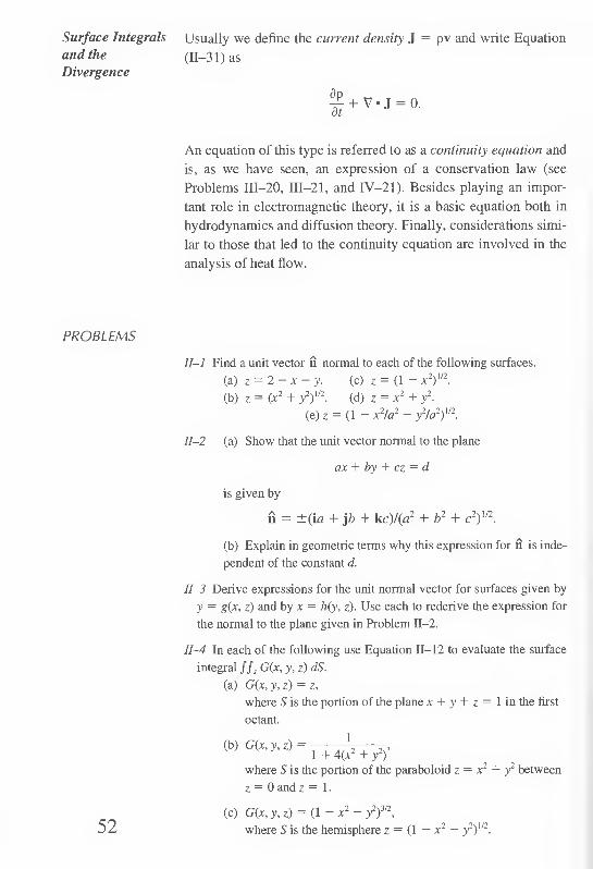
1-1 Using arrows of the proper magnitude and direction, sketch each of
the following vector functions:
(a) iy + jx (e) jx
(b) (i + j)/V2. (f) (iy + jxyVx2 + y2, (x y) + (0, 0).
(c) ix - jy. (g) iy + jxy.
(d) iy. (h) i + jy. 8

Problems 1-2 Using arrows, sketch the electric field of a unit positive charge situ¬
ated at the origin. [Note: You may simplify the problem by confining
your sketch to one of the coordinate planes. Does it matter which plane
you choose?]
1-3 (a) Write a formula for a vector function in two dimensions
which is in the positive radial direction and whose magnitude
is 1.
(b) Write a formula for a vector function in two dimensions
whose direction makes an angle of 45° with the .(-axis and whose
magnitude at any point (x, y) is (x + y)2.
(c) Write a formula for a vector function in two dimensions
whose direction is tangential (in the sense of the example on page
5) and whose magnitude at any point (x, y) is equal to its distance
from the origin.
(d) Write a formula for a vector function in three dimensions
which is in the positive radial direction and whose magnitude
is 1.
1-4 An object moves in the xy-plane in such a way that its position vec¬
tor r is given as a function of time t by
r = ia cos iat + jb sin oot,
where a, b, and to are constants.
(a) How far is the object from the origin at any time f?
(b) Find the object’s velocity and acceleration as functions of
time.
(c) Show that the object moves on the elliptical path
1-5 A charge + 1 is situated at the point (1, 0, 0) and a charge —1 is sit¬
uated at the point (—1, 0, 0). Find the electric field of these two
charges at an arbitrary point (0, y, 0) on the y-axis.
1-6 Instead of using arrows to represent vector functions (as in Prob¬
lems 1-1 and 1-2), we sometimes use families of curves called field
lines. A curve y = y(x) is a field line of the vector function F(x, y) if
at each point (jc0, y0) on the curve, F(x0, y0) is tangent to the curve (see
the figure).
9 (*o. y0)
X

Introduction,
Vector Functions,
and Electrostatics
(a) Show that the field lines y = y(x) of a vector function
F(Jt, y) = iFr(x, y) + jFy(x, y)
are solutions of the differential equation
dy _ F?(x, y)
dx Fx(x, y)'
(b) Determine the field lines of each of the functions of Problem
1-1. Draw the field lines and compare with the arrow diagrams of
Problem 1-1.
10

Chapter II
Surface Integrals and the Divergence
Oh, could I flow tike thee, and make
thy stream
My great example....
Sir John Denham
Gauss' Law
Since the electrostatic field is so important a quantity in electro¬
statics, it follows that we need some convenient way to find it,
given a set of charges. At first glance it might appear that we
solved this problem before we even stated it, for, after all, do not
Equations (1-4) and (1-7) provide us with a means of finding E?
The answer is, in general, no. Unless there are very few charges
in the system and/or they are arranged simply or very symmetri¬
cally, the sum in Equation (1-4) and the integral in Equation
(1-7) are usually prohibitively difficult—and frequently impos¬
sible—to perform. Thus, these two equations provide what is 11

Surface Integrals
and the
Divergence
usually only a “formal” solution1 to the problem, not a practical
one, and we must cast about for some other way to calculate the
field E.
In the course of this casting about, we come inevitably to that
remarkable relation known as Gauss’ law. We say “inevitably”
because it is hard to think of any other expression in elementary
electricity and magnetism containing the electric field [apart, of
course, from Equations (I^f) and (1-7), which we have already
rejected]. Gauss’ law is
jjE-*ds = f <n-D
If you don’t understand this equation, don’t panic. The left-hand
side of this equation is an example of what is called a surface
integral, an important concept in vector calculus and one that is
probably new to you. The integrand of this integral is the dot
product of the electric field and the quantity n, which is called a
“unit normal vector” and is probably also unfamiliar. We are
about to discuss both surface integrals and unit normal vectors
in excruciating detail, and one of our main reasons for quoting
Gauss’ law at this point in our narrative is to motivate this
discussion.
We won’t stop here to derive Gauss’ law, since the derivation
wouldn’t mean much to you until you have read the next few sec¬
tions. Then you can consult almost any text on electricity and
magnetism for the gory details. And if you can contain yourself,
wait until we’ve discussed the divergence theorem (pages 45-52),
after which you will be able to derive Gauss’ law easily (see
Problem 11-27).
The Unit Normal Vector
One of the factors in the integrand in Gauss’ law [Equation
(II—1)] is a quantity designated n and called the unit normal vec¬
tor. This quantity is part of the integrand in most if not all of the
surface integrals we’ll encounter; furthermore, as we’ll see, it
plays an important role in the evaluation of surface integrals even
12 The word “formal” in this context is a euphemism for “useless.”

The Unit Normal
Vector
when it does not appear explicitly. Thus, before discussing sur¬
face integrals themselves, we’ll dispose of the questions of how
this vector function is defined and calculated.
The word “normal” in the present context means, loosely
speaking, “perpendicular.” Thus, a vector N normal to the xy-
plane is clearly one parallel to the z-axis (Figure II—1), while a
Figure II-1
vector normal to a spherical surface must be in the radial direction
(Figure II—2). To give a precise definition of a vector normal to a
Figure II—2
surface, consider an arbitrary surface S, as shown in Figure II—3.
Construct two noncollinear vectors u and v tangent to S at some
point P. A vector N which is perpendicular to both u and v at P is,
by definition, normal to S at P. Now, as we know, the vector 13

Surface Integrals
and the
Divergence
N A
Figure II—3
product of u and v has precisely this property; it is perpendicular
to both u and v. Thus, we may write N = u X v. To make this a
unit vector (that is, one whose length is 1) is simple: we just di¬
vide N by its magnitude N. Thus,
/s N u X v n = = i-r
N | u X v |
is a unit vector normal to S at P.
To find an expression for n, we consider some surface S given
by the equation z = f(x, y); see Figure II-4. Following the proce-
Figure II-4
dure suggested by the preceding discussion, we’ll find two vec¬
tors u and v whose cross product will yield the required normal
vector n. For this purpose let’s construct a plane through a point
P on S and parallel to the xz-plane, as shown in Figure II-4. This
plane intersects the surface S in a curve C. We construct the vec- 14

The Unit Normal
Vector
tor u tangent to C at P and having an x-component of arbitrary
length ux. The z-component of u is (df/dx)ux; in this expression
we use the fact that the slope of u is, by construction, the same as
X
Figure II—5
that of the surface S in the x-direction (see Figure II-5). Thus,
, df U = 1M' + kl to
u. - + k (H-2)
To find v, the second of our two vectors, we pass another plane
through the point P on S, but in this case parallel to the yz-plane
(Figure II—6). It intersects S in a curve C', and the vector v can
Figure H-6
now be constructed tangent to C' at P with a y-component of arbi¬
trary length vy. Arguing as above, we have
v=jyr + k U;b = J + k^ 15 (H-3)

Surface Integrals and the Divergence
Using the two vectors u and v as given in Equations (II—2) and
(II—3), we now construct their cross product. The result.
U X V = + k UYV
is a vector, which as we stated above, is normal to S at P. To
make a unit vector of this, we divide it by its magnitude to get
n(x, y, z) u X v
u X v (II—4)
This, then, is the unit vector normal to the surface z = f(x, y) at
the point (x, y, z) on the surface.2 Note that it is independent of the
two arbitrary quantities ux and vy.
A couple of examples may be in order here. First a trivial one:
What is the unit vector normal to the xy-plane? The answer, of
course, is k (see Figure II—1). Let’s see how Equation (II-4) pro¬
vides us with this answer. The equation of the xy-plane is
z =f(*,y) = 0,
whence we have the profound observations
dfldx = 0 and d//dy = 0.
Substituting these in Equation (II-4), we get n = k/VT = k, as
advertised.
As a second example, consider the sphere of radius 1 centered
at the origin (Figure II—2). Its upper hemisphere is given by
z =f(x,y) = (1 - x2 - y2)m,
2 The uniqueness of our result [Equation (II-4)] may be questioned on two counts.
The first of these is a sign ambiguity: If n is a unit normal vector, so is — n. The
matter of which sign to use is discussed below. The second question arises from
the fact that the two tangent vectors u and v used in determining n are rather spe¬
cial, since each is parallel to one of the coordinate planes. Would we get the same
result using two arbitrary tangent vectors? This issue is considered in Problem
IV-26, where it is shown that n as given by Equation (II-4) is, apart from sign,
indeed unique.

Definition of
Surface Integrals
whence
V dx
x z and
d/ dy
y z■
Using these in Equation (II-4) leads to
n =
ix z k ix + jy + kz
Vx2 + y2 + z2 ix + jy + kz.
where we have used the equation of the unit sphere x2 + y2 +
z2 = 1. This is, as expected, a vector in the radial direction (see
Figure II—2). To show that its length is 1, we observe that n •
n = x2 + y2 + z2 = 1 •
With the matter of the unit normal vector now disposed of, we
turn to our next task, a discussion of surface integrals.
Definition of Surface Integrals
We now define the surface integral of the normal component of a
vector function F(x, y, z). This quantity is denoted by
F • n dS, (II—5)
and as you can see, Gauss’ law [Equation (II—1)] is expressed in
terms of just such an integral. Let z = f(x, y) be the equation of
some surface. We’ll consider a limited portion of this surface,
which we designate S (see Figure II—7). Our first step in formulat-
17 Figure II—7

Surface Integrals
and the
Divergence
ing the definition of the surface integral (II—5) is to approximate S
by a polyhedron consisting of N plane faces each of which is tan¬
gent to S at some point. Figure II—8 shows how this approximat-
Figure II—8
ing polyhedron might look for an octant of a spherical shell. We
concentrate our attention on one of these plane faces, say the Zth
one (Figure II—9). Let its area be denoted AS, and let (xh yh zi) be
Figure II—9
the coordinates of the point at which the face is tangent to the sur¬
face S. We evaluate the function F at this point and then form its
dot product with n,, the unit vector normal to the Zth face. The re¬
sulting quantity, F(x,, yh zi) • n,, is then multiplied by the area A.S',
of the face to give
Flx,, y„ zi) • n, AS,.
We carry out this same process for each of the N faces of the ap¬
proximating polyhedron and then form the sum over all N faces:
^ F(x;, yh zi) • n, AS,. 1=1 18

Definition of
Surface Integrals
The surface integral (II—5) is defined as the limit of this sum as
the number of faces, N, approaches infinity and the area of each
face approaches zero.3 Thus,
F*n dS N
lim 2 F(*/> yi< Zi) * »/ A5;. (V—1= J
each AS,—»0
(II—6)
If we want to cross all the f s and dot all the V s, this integral,
strictly speaking, should be written
y, z) • n(x, y, z) dS
since both F and n are, in general, functions of position. We pre¬
fer, and where possible will use, the less cluttered notation
F-n dS
with the arguments of the functions understood.
The surface S over which we integrate a surface integral can be
one of two kinds: closed or open. A closed surface, such as a
spherical shell, divides space into two parts, an inside and an out¬
side, and to get from inside to outside, you must go through the
surface. An open surface, such as a flat piece of paper, does not
have this property; it is possible to get from one side of the sheet
to the other without going through it. The definition of surface in¬
tegrals given in Equation (II—6) applies equally well to both
closed and open surfaces. However, the surface integral is not
well defined until we specify which of the two possible directions
of the normal we are to use (see Figure II—10). In the case of an
Figure II-10
3 The statement “each AS/ 0” is not quite precise. The area of a rectangular
patch, for example, might tend to zero because its width decreases while its length
remains fixed. This would not be acceptable. Here and elsewhere we must inter¬
pret “each AS, —* 0” to mean that all linear dimensions of the /th patch tend to
19 zero.

Surface Integrals
and the
Divergence
open surface, the direction must be given as part of the statement
of the problem. In the case of a closed surface, there is a gentle¬
men’s agreement which specifies the direction once and for all:
the normal is chosen so that it points outward from the volume
enclosed by the surface.
The integral in Gauss’ law [Equation (II—1)] is taken over a
closed surface. Gauss’ law, in fact, says that the surface integral
of the normal component of the electric field over a closed surface
is equal to the total (net) charge enclosed by the surface, divided
by e0. Below (pages 33-37 and Problems II—11,11-12, and 11-13)
we’ll see how, when the charges are arranged neatly and symmet¬
rically, Gauss’ law can be used to determine the electric field. But
the thrust of our whole discussion will be to subject Gauss’ law to
a series of harrowing adventures which eventually transform it
into an expression useful for finding E even when we don’t have
symmetry to help us.
Sometimes we encounter surface integrals which are a little
simpler than the kind we’ve just defined, although basically they
are almost the same. These are surface integrals of the form
y, z) dS, (H-7)
where the integrand G(x, y, z) is a given scalar function rather
than the dot product of two vector functions as in (II—5) and
(II—6). We go about defining this kind of surface integral much
as we did above: we approximate S by a polyhedron, form the
product G(xh yh Zi) ASh sum over all faces, and then take the
limit:
, y, z) dS N
lim 2 G(*/> 37- */) ASh /= 1
each AS,—>0
(ii—8)
As an example of this kind of surface integral, suppose we have a
surface of negligible thickness with surface density (that is, mass
per unit area) a(x, y, z), and we wish to determine its total mass.
Approximating this surface by a polyhedron as above, we recog¬
nize that a(xh yh zi) AS, is approximately the mass of the /th face
of the polyhedron and that
N
S ct(.x„ yh zi) AS, 1= 1 20

Evaluating is approximately the mass of the entire surface. Taking the limit
Surface Integrals
lim 2 a(xb yi> Z;) AS, = [l a(x’ z) ^S, /=1 J
each AS,—>0
we get the total mass of the surface.
An example of an even simpler surface integral of this kind is
//,* This integral is taken as the definition of the surface area of S.
Evaluating Surface Integrals
Now that we have defined surface integrals, we must develop
methods to evaluate them, and that will be our task here. For sim¬
plicity we’ll deal with surface integrals of the form (II—7), where
the integrand is a given scalar function, rather than the slightly
more complicated form (II—5). There will be no loss of generality
in doing this for all our results can be made to apply to integrals
of the form (II—5) just by replacing G(x, y, z) everywhere by
F(x, y, z) • n.
To evaluate the integral
J J G(x, y, z) dS
over a portion S of the surface z = /(x, y) (see Figure II—11), we
go back to the definition of the surface integral [Equation (II—8)].
21 Figure II-11

Surface Integrals
and the
Divergence
Figure 11-12
Our strategy will be to relate AS) to the area AR, of its projection
on the xy-plane, as shown in Figure 11-12. Doing so, as we’ll see,
will enable us to express the surface integral over S in terms of an
ordinary double integral over R, which is the projection of S on
the xy-plane, as shown in Figure II—11.
Relating AS, to AR: is not difficult if we recall that AS, (like the
area of any plane surface) can be approximated to any desired de¬
gree of accuracy by a set of rectangles as shown in Figure 11-13.
Figure 11-13
For this reason we need only find the relation between the area of
a rectangle and its projection on the xy-plane. Thus, consider a
rectangle so oriented that one pair of its sides is parallel to the
xy-plane (Figure 11-14). If we call the lengths of these sides a, it’s
clear that their projections on the xy-plane also have length a. But
the other pair of sides, of length b, have projections of length b',
and in general, b and b' are not equal. Thus, to relate the area of
the rectangle ab to the area of its projection ab', we must express 22

Evaluating
Surface Integrals
Figure 11-14
b in terms of b'. This is easy to do, for if 0 is the angle shown in
Figure 11-14, we have b = b'!cos 0, and so
cos 0 '
If we let n denote the unit vector normal to our rectangle, then we
can readily convince ourselves that cos 0 = n • k where k, as al¬
ways, is the unit vector in the positive z-direction. Thus,
Since the area AS, can be approximated with arbitrary accuracy
by such rectangles, it follows that
A S,= A R,
n,
where, of course, n, is the unit vector normal to the /th plane
surface.
We can now rewrite the definition of the surface integral
[Equation (II—8)] as
n AR
lim (II—9) w->co /=1 ii/*k
each AR,—*0
where the statement “each AS, —» 0” has been replaced by the
equivalent but now more appropriate “each AR, —» 0.” We are 23

Surface Integrals
and the
Divergence
now obviously well on the road to rewriting the surface integral
over S as a double integral over R. In fact,
N
lim N-* co l= i
each A/?,—>0
G(x„ yh zj)
n, • k AR,= G(x, y, z)
n(*, y, z) • k dx dy. (11-10)
where n(x, y, z) is the unit vector normal to the surface S at the
point (x, y, z). This is a double integral over R even though it
does not quite look like one. What appears to spoil it is that
nasty z in G and n; a double integral over a region in the
Ay-plane clearly has no business containing any z’s. But the
z-dependence is spurious because (x, y, z) are the coordinates of
a point on 5, and so z = /(x, y). Hence, at the expense of making
the integral look even fiercer than it already does in Equation
(II—10), we can eliminate the apparent z-dependence of the inte¬
grand and write
G[x,y,f(x,y)] J J -r-dx dy n[x,y,/(x,y)]-k
(H-ll)
The faint of heart can take courage; in most cases this integrand
reduces quickly to something much simpler and pleasanter look¬
ing—a fact we will demonstrate by example below. At this point
we introduce the expression for the unit normal vector [Equation
(II—4)]. We find
Vl + (df/dx)2 + (df/dy f ’
and so Equation (II-11) becomes
G[x, y,f(x, y)]
(H-12)
Thus, the surface integral of G(x, y, z) over the surface S has been
expressed as a double integral of a messy-looking function over
the region R, the projection of S in the xy-plane. As we remarked
above, in practice the integral is usually much less ghastly than it 24

Evaluating
Surface Integrals
appears written out in Equations (II—11) or (11-12). You will see
this in the examples we now give.
Let’s first compute the surface integral
+ z) dS
where S is the portion of the plane x + y + z — 1 in the first oc¬
tant shown in Figure II-15(a). The projection of S on the ry-plane
Figure II—15(a)
is the triangle R shown in the figure. The equation of S can be
written
z — fix, y) = 1 - x-y
from which we get
dx dy
so that
= V3.
Hence
ff (x + z)dS = V3 //, (x + z) dx dy =
(x + 1 — x — y) dx (1 - y) dx dy. 25

Surface Integrals
and the
Divergence
where we have used z = \ — x — y. This is a simple double inte¬
gral with value 1/V3, as you should be able to verify.
As a second example let’s compute the surface integral
where S is the octant of the sphere of radius 1 centered at the ori¬
gin as shown in Figure II—15(b). The projection of S on the
Figure II—15(b)
xy-plane (that is, R) is the area enclosed by the quarter circle. The
equation of S is x1 + y2 + z2 = 1, or
Z =f(x,y) = +Vl - x2 - y2.
It follows then that
V dx -f and ¥ = _y
dy Z'
so that
|Vx2 + y2 + z2 = 1 z ’
where we have used x2 + y2 + z2 = 1. Hence,
z dx dy. 26

Evaluating
Surface Integrals
Substituting for z in terms of x and y, we get
J J z2 dS = J J V1 — x1 — y1 dx dy.
This is an ordinary double integral, and you should verify that its
value is ir/6. [Suggestion: Convert to polar coordinates: x = r cos
0, and y = r sin 0. The integration is then trivial.]
It should be emphasized that the foregoing discussion was
based on the assumption that the surface S is described by an
equation of the form z = fix, y); in such a situation a surface inte¬
gral is converted into a double integral over a region in the
jcy-plane. But it may happen that a given surface is more conve¬
niently described by an equation of the form y = g(x, z) as in Fig¬
ure II—16(a). If this is so, then
Figure U-16(a)
where R is a region in the vz-plane. Similarly, if we have a surface
described by x = h(y, z), as in Figure II—16(b), then we use
G[h(y, z), y, z] dydz, 27

Surface Integrals
and the
Divergence
Figure H-16(b)
where R in this case is a region in the yz-plane. Finally, a surface
may have several parts, and it may then be convenient to project
different parts on different coordinate planes.
To evaluate surface integrals of the form (II—5), that is.
F • n dS,
we merely replace G by F • n in Equation (11-12) to get
F • n dS =
If we now use Equation (II-4) to write this out in detail, we find
that the square root factor cancels and we get
ffsF'SdS = fl{-Fx[x,y,f(x,y)]^ - Fv[x, y,f(x, y)] + F.[x, y,f(x, y)]| dx dy. (11-13)
We leave it to the reader to write down the analogous formulas
when the surface S is given by y = g(x, z) or x = h(y, z), which must
be projected onto regions in the xz- and yz-planes, respectively.
This last equation [Equation (11-13)] is enough to make strong
men weep, but, as before, in most calculations it quickly reduces
to something quite tame. For example, suppose we wish to calcu¬
late ffs F • n dS, where F(x, y, z) = iz ~ jy + kx and S is the por¬
tion of the plane
28 x + 2y + 2z = 2

Evaluating
Surface Integrals
Figure II-17(a)
bounded by the coordinate planes, that is, the triangle reclining
gracefully in Figure II-17(a). The normal vector n is chosen so
that it points away from the origin as shown in Figure II—17(a),
and we’ll project S onto the xy-plane. We have
z =f(x,y) = 1 - | ~y.
and so
Of _ _i =
dx 2' dy
We also have
Fx = z = 1 - 2 - y> Fy= -y, Fz = x.
Hence
Jfr.n dS
1 x
l~i~y -ill- '//if-T-'-iW
(-|)+y(-l)+x dxdy
29
The region R over which the integral must be taken is shown in
Figure U-17(b). The problem has thus been reduced to the compu-

Surface Integrals
and the
Divergence
Figure II-17(b)
tation of a rather simple double integral, and you should carry out
the integration yourself (the answer is |).
As a second example, suppose
F(x, y, z) -ixz + kz2
For S let’s take the octant of the spherical surface shown in Figure
11-15. Then z - f(x,y) = Vl — x2 — y2; and we have already
shown (see page 25) that
dl dx
-f and tf_= _y_ dy z
Thus
fl*A dS
-xz\ -'jl + zr Z2j dx dy = J J (x2 + 1 — x2 — y2)dx dy
~ J J (1 — y2)dx dy = J J dxdy — J J y2 dx dy
where R, we recall, is the quarter-circle shown in Figure 11-15.
The first integral in the last equality above is just the area of the
quarter-circle of radius 1, and is therefore equal to tt/4. The sec¬
ond integral can be done by introducing polar coordinates. We get
f f y2 dxdy = [ f r2 sin2 0r dr J Jr Jo Jo
r ti/2 r l
= I sin2 0 d6 r3 dr J o J o
dd
30

Flux Both the r and 0 integrals here are elementary, and you should
have no trouble showing that this expression is equal to tt/16.
Thus ffs F • n dS — tt/4 — tt/16 = 3tt/16.
Flux
An integral of the type
(11-14)
is sometimes called the “flux of F.” Thus Gauss’ law [Equation
(II—1)] states that the flux of the electrostatic field over some
closed surface is the enclosed charge divided by e0.
It is useful in obtaining a geometrical feeling for some aspects
of vector calculus to understand the significance of the word flux
(Latin for “flow”) used in this context. For this purpose let us con¬
sider a fluid of density p moving with velocity v. We ask for the
total mass of fluid that crosses an area AS perpendicular to the di¬
rection of flow in a time At. Clearly, all the fluid in the cylinder of
length v At with the patch AS as base will cross AS in the interval
At (Figure 11-18). The volume of this cylinder is v At AS, and it
Figure 11-18
contains a total mass pv At AS. Dividing out the At will give the
rate of flow. Thus,
Rate of flow) . „
through AS j'p045-
Now let us consider a somewhat more complicated case in
which the area AS is not perpendicular to the direction of flow
(Figure 11-19). The volume containing the material that will flow 31

Surface Integrals
and the
Divergence C <■ vAt ■>
Figure 11-19
through AS in time At is now just the volume of the little skewed
cylinder shown in the diagram. The volume is v At AS cos 0, where
0 is the angle between the velocity vector v and n, the unit vector
normal to AS and pointing outward from the skewed cylinder. But
v cos 0 = v • n. So, multiplying by p and dividing by At, we get
/ Rate of flow
\ through AS = pv • n AS.
Finally, consider a surface S in some region of space containing
flowing matter (Figure 11-20). Approximate the surface by a poly¬
s' ^ y
Figure 11-20
hedron. By the above argument, the rate at which matter flows
through the Zth face of this polyhedron is approximately
PC*/, yi, z,)v(x„ y„ z,) • n, AS,.
Here, of course, (xh yh z,) are the coordinates of the point on the Zth
face at which it is tangent to S, and n, is the unit vector normal to
the Zth face. Summing over all the faces and taking the limit, we get
[ Rate of flow
\ through S , y, z)\(x, y,z)'n dS.
32 If S happens to be a closed surface and there is a net rate of flow
out of the volume it encloses, then you can convince yourself that

Using Gauss’
Law to Find
the Field
Using Gauss
this integral will be positive, and if there is a net rate of flow in,
the integral will be negative.
If in this last equation we put
F(x, y, z) = pU, y, z)v(x, y, z),
the integral is seen to be formally identical with that in Equation
(11-14). For this reason any integral of the form (11-14) is called
“the flux of F over the surface S,” even when the function F is not
the product of a density and a velocity! The reason for stressing
this point about flux is that, misnomer though it may be, it
nonetheless gives a good geometric or physical picture of Gauss’
law: The electric field “flows” out of a surface enclosing charge,
and the “amount” of this “flow” is proportional to the net charge
enclosed. Warning: This is not to be taken literally; the electric
field is not flowing in the sense in which fluid flows. It is merely
picturesque language intended to aid us in understanding the
physics in Gauss’ law.
Law to Find the Field
Having rejected the two expressions for E [Equations (1-4) and
(1-7)], we find that the only candidate left for providing us with a
good general method for calculating the field is Gauss’ law. At
first glance it does not appear to be a very likely candidate be¬
cause, unlike Equations (1-4) and (1-7), it is not an explicit ex¬
pression for E. That is, it does not say “E equals something.”
Rather, it says “The flux of E (the surface integral of the normal
component of E) equals something.” Thus, to use Gauss’ law, we
must “disentangle” E from its surroundings. Despite this, there
are situations in which Gauss’ law can be used to find the field, as
an example will now show.
Consider a point charge q placed at the origin of a coordinate
system. Symmetry considerations tell us two things about its elec¬
tric field: (1) It must be in the radial direction (that is, it must
point directly toward, or directly away from, the origin), and (2) it
must have the same magnitude at all points on the surface of a
sphere centered at the origin. Stating this in symbols, we have
E = erE(r), where er = rIr is a unit vector in the radial direction.
Thus, Gauss’ law becomes
n dS = q/e0. 33

Surface Integrals If, for the surface S, we now choose a spherical shell of radius
and the r centered at the origin, a little thought will convince you that
Divergence n = gr, so that n • er = 1 and we get
E(r) dS = q/e0.
This integral is trivial to perform if we recognize that r is a con¬
stant over the spherical surface S. This means that E(r) is also a
constant on S and we get4
dS = 4tt r2E(r) = q/e0,
whence
E(r) = l q
4-Tre0 r2
and
E(r) = erE(r) = q
4rre0 r2 ’
in agreement with Equation (1-2).
We can see from this example how heavily we depend on sym¬
metry when using Gauss’ law to obtain the field. In fact, to use
Gauss’ law in the form given in Equation (II—1) requires even
more symmetry and simplicity than Equations (1-4) and (1-7).
The blunt truth is that this form of the law yields the electric field
in a grand total of three situations (and combinations thereof):
(1) a spherically symmetric distribution of charge (of which the
point charge considered above is a special case), (2) an infinitely
long cylindrically symmetric distribution (including the case of an
infinitely long uniformly distributed line of charge), and (3) an in¬
finite slab of charge (including as a special case an infinite uni¬
formly charged plane).5 The real value of Equation (II—1) is that it
can be twisted and beaten into a more useful form.
4 Shortcuts like this often make it possible to evaluate surface integrals without
using all the paraphernalia we discussed above. Further examples are given in
Problem II—10.
5 Examples of these are given in Problems H-l 1,11-12, and 11-13.

Using Gauss’
Law to Find
the Field
What is it about Equation (II—1) that makes it difficult to find
E? To answer this question, suppose we are doing a numerical
calculation on a computer and wish to evaluate //5 E • n dS. The
standard procedure for dealing with integrals numerically is to ap¬
proximate them as sums, a rather obvious thing to do since an in¬
tegral, after all, is the limit of a sum. Thus, suppose we divide the
surface S into, say, 10 patches. We then have as an approximation
to Equation (II—1)
10
2 E, • n, AS, — q/e0, i= 1
where E, is the value of E, and n, is the unit normal, somewhere
on the /th patch. There is little or no hope of finding E from this:
it is one equation in the 10 unknowns E1; E2,. . ., E10. Further¬
more, it is probably not very accurate. To improve the accuracy,
we might make 100 subdivisions rather than just 10 to get
100
2 E, • n, AS, = q/e0. i=i
Much more accurate! And much more hopeless too, because this
is one equation in 100 unknowns. Even more accurate (and more
hopeless) is
II E • n dS = q/e0,
which is one equation in infinitely many unknowns. These un¬
knowns are, of course, the values of E • n at every one of the infi¬
nitely many points of the surface S.6
We have now isolated the trouble with Equation (II—1): it in¬
volves an entire surface and therefore the value of E • n at infi¬
nitely many points. If, somehow, we could deal with the “flux at a
single point” (whatever that may mean!) rather than the flux
through a surface, perhaps then Gauss’ law might yield something
tractable. How might we arrange this? For simplicity let us sur¬
round some point P by a set of concentric spherical shells 5,, S2,
S3, and so on (Figure 11-21), and calculate the flux <&,, $2, *£3.
35
6 The reason Gauss’ law yields the expression for the field of a point charge exam¬
ined above is that symmetry in that case shows that the infinitely many unknowns
are all equal. This turns Gauss’ law into one equation in one unknown.

Surface Integrals
and the
Divergence
Figure 11-21
and so on, through each shell. We might then attempt to define the
“flux at the point P” as the limiting value approached by the se¬
quence of fluxes calculated this way over smaller and smaller
shells centered at P.
This sounds good; it has a heartening “mathematical” ring to it.
Unfortunately, it does not work because (assuming the charge
density is finite everywhere) the sequence of fluxes, calculated as
described above, approaches zero for any point P. This is fairly
obvious since it is merely the statement that the flux through a
surface tends to zero as the surface shrinks to a point. Since our
objective was to find a way to determine the flux at a point, and
thereby learn something about the field at that point, and since we
get zero at any point no matter what the field there may be, we
have obviously not obtained what we want.
It is useful to give a physicist’s rough-and-ready proof of the
fact that the flux goes to zero as the surface shrinks down to a
point, for even though this fact may be obvious, the proof will
suggest how to pull this chestnut out of the fire. For this purpose
we note that if pAV, denotes the average density of electric charge
[Equation 1-5] in some region of volume AV, then the total
charge in AV is pAl, AV. Thus Gauss’ law [Equation (II-l)] may
be written
36
E • n dS = pAV, AV/e0, (H-15)
where, as indicated in Figure 11-22, the surface integral is taken
over the surface S that encloses the volume AV. From this expres¬
sion [Equation (11-15)] we can see the validity of our assertion;
As S —* 0, the enclosed volume A V must, of course, also approach

The Divergence AV
S
Figure 11-22
zero. Thus, the flux also tends to zero and the assertion is proved.7
Not only have we given a proof, but (and this is the point) we can
now isolate a quantity that does not vanish as S —» 0. Dividing
Equation (11-15) by AV, we get
^ J J^E • n dS = Pav/€q.
This expression, awkward and unappealing though it may be, is
nonetheless close to what we are after, even though it still involves
an integral of E over an entire surface. For if we now take the limit
as S shrinks to zero about some point in AV whose coordinates are
(x, y, z), then, as we see from Equation (1-6), the average density
Pav approaches p(x, y, z), the density at (x, y, z), and we get
lim a!7 [ f E * n dS = p(*, y, z)/e0. (11-16) AV—>0 /XV J J5
about (x,yj)
This expression is admittedly downright hideous, and whether it
will be of any practical use whatever depends on our being able to
pound the left-hand side into a form that looks and acts at least
half-civilized. We turn to this task now.
The Divergence
Let us consider the surface integral of some arbitrary vector func¬
tion F(x, y, z):
F • n dS.
37 7 This line of reasoning and the conclusion must be altered if the system contains
point charges.

Surface Integrals
and the
Divergence
We shall be interested in the ratio of this integral to the volume
enclosed by the surface S as the volume shrinks to zero about
some point, for that is exactly the type of quantity that appears in
Equation (11-16). This limit is important enough to warrant a spe¬
cial name and notation. It is called the divergence of F and is des¬
ignated div F. Thus,
div F = lim f [ F • n dS. (11-17) av->o A V J Js
about (x,y,z)
This quantity is clearly a scalar. Furthermore, it will, in general,
have different values at different points (x, y, z). Thus the diver¬
gence of a vector function is a scalar function of position.
Equation (11-16) can now be written
div E = p/e0. (11-18)
At this stage, however, our fancy new notation has only a cos¬
metic value, helping to beautify an ugly equation. Whether it has
any practical value as well is the matter taken up in the following
discussion in which we actually calculate the limit of the ratio of
flux to enclosed volume and find that it can be expressed reason¬
ably simply in terms of certain partial derivatives. Before turning
to this calculation, however, it’s worth mentioning that if we take
our new terminology literally, we can interpret Equation (11-18)
to mean that the field “diverges” from a point, and how much it
diverges, so to speak, depends on how much charge there is at
that point as represented by the density there.
Our next order of business is to find the reasonably simple ex¬
pression for the divergence of a vector function promised above.
Thus, consider a small rectangular parallelepiped8 with edges of
length Ax, Ay, and Az parallel to the coordinate axes (Figure
11-23). Let the point at the center of the little cuboid have coordi¬
nates (x, y,z)- We calculate the surface integral of F over the sur¬
face of the cuboid by regarding the integral as a sum of six terms,
one for each cuboid face. We begin by considering the face
marked 5] in the figure. We want
38 8 Henceforth we’ll refer to this as a “cuboid,” a made-up term that takes less time
and space than the sesquipedalian “rectangular parallelepiped.”
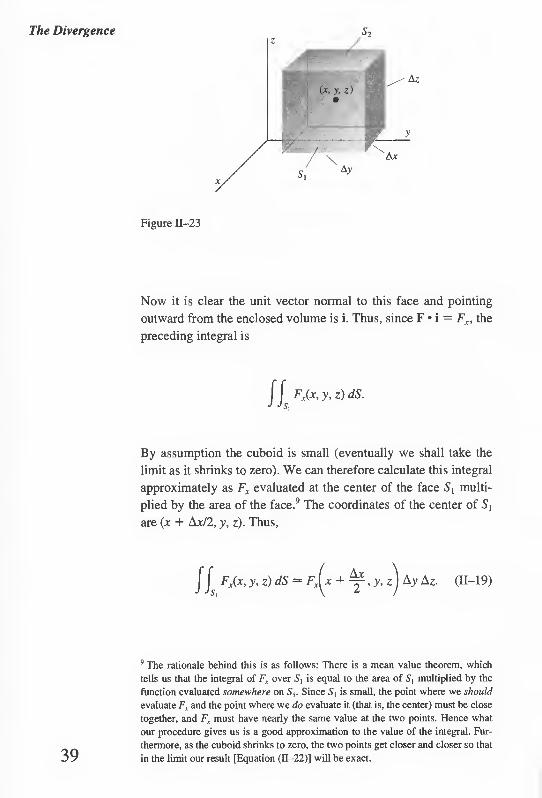
Figure 11-23
Now it is clear the unit vector normal to this face and pointing
outward from the enclosed volume is i. Thus, since F • i = Fx, the
preceding integral is
y, z) dS.
By assumption the cuboid is small (eventually we shall take the
limit as it shrinks to zero). We can therefore calculate this integral
approximately as Fx evaluated at the center of the face S, multi¬
plied by the area of the face.9 The coordinates of the center of 5,
are (x 4- Ax/2, y, z). Thus,
II, Fx(x, y, z) dS — Fx , Ax
* + T,y,z Ay Az. (11-19)
9 The rationale behind this is as follows: There is a mean value theorem, which
tells us that the integral of Fx over S, is equal to the area of S, multiplied by the
function evaluated somewhere on S,. Since 5, is small, the point where we should
evaluate Fx and the point where we do evaluate it (that is, the center) must be close
together, and Fx must have nearly the same value at the two points. Hence what
our procedure gives us is a good approximation to the value of the integral. Fur¬
thermore, as the cuboid shrinks to zero, the two points get closer and closer so that
in the limit our result [Equation (11-22)] will be exact. 39

Surface Integrals The same kind of reasoning applied to the opposite face S2
and the [whose outward normal is — i and whose center is at (x - Ax/2, y.
Divergence z)] leads to
F'hdS FxdS
Ax 2 '
y,z) Ay Az. (11-20)
Adding together the contributions of these two faces [Equations
(11-19) and (11-20)], we get
Ax
2 Ay A z
, Ax x + ~Y,y,z - FA x-=- Ax
2 y.z
Ax Ax Ay Az.
Recognizing that Ax Ay Az = AV, the volume of the cuboid, we have
AVJJSi+S2 F*n dS
Fx (x + ^ > y> z J ~ Fx ^x — ^, y, z
Ax (11-21)
We now must take the limit of this as AV approaches zero.10 But,
of course, as AV goes to zero, so do each of the sides of the
cuboid. Thus, on the right-hand side of Equation (11-21) we can
write lim4,._0 in place of limiv_^0, and we find
lim At/ av—*o AV Lff tV J Js,+s2
F*n dS
= lim ■ Ax-*0
FAx + Ax
>y,z x — Ax 2 :
Ax
dF\ dx
40 10 Note that we have postponed calculating the contributions from the other four
faces of the cuboid.

The Divergence evaluated at (x, y, z). This last equality follows from the definition
of the partial derivative. It should come as no surprise that the
other two pairs of faces of the cuboid contribute dFy/dy and
dFJdz. Thus,
lim — av-^o AV II F • n dS =
dFx dF SF. —- q-- h--
dx dy dz '
The limit on the left-hand side of this last equation, as we have al¬
ready remarked, is the divergence of F [Equation (11-17)]. Thus
we have just demonstrated that
div F = dF, BF, dF,
dx + dy dz' (11-22)
It can be shown that this result is independent of the shape of the
volume used to obtain it (see Problem 11-17).
Using Equation (11-22) to find the divergence of a vector func¬
tion is a straightforward matter, but we’ll give an example just for
the record. Consider the function
F(jc, y, z) = ix2 + jxy + kvz.
We have
dF- and —t — = y.
dz
Thus,
div F = 2x + x + y = 3x + y.
Returning now to the electrostatic field, we combine Equations
(11-18) and (11-22) to get
BE. dE dE- —- q-- -I-5 dx dy dz
p/e0. (11-23)
This equation, which is much more general than our derivation of
it suggests, is one of Maxwell’s equations and is completely
equivalent to Gauss’ law [Equation (II—1)]. It is sometimes called
the “differential form” of Gauss’ law.
We have now arrived at our goal (almost!), for we have related a
property of the electrostatic field at a point (that is, its divergence) to
a known quantity (the charge density) at that point. In all fairness it 41
Surface Integrals should be said that Equation (11-23) can in a sense be regarded as a
and the single (differential) equation in three unknowns (Ex, Ey, E7) and for
Divergence this reason is not often used in this form to find the field. It turns out,
however, that the three components of E can be related to each other
very elegantly; when we develop that relationship, we shall return to
this question of finding a convenient means of calculating E.
The Divergence in Cylindrical and Spherical Coordinates
One often sees Equation (11-22) given as the definition of the di¬
vergence of the vector function F. While this is certainly accept¬
able, we much prefer to define the divergence as the limit of flux
to volume as stated in Equation (11-16). Equation (11-22) is then
merely the form the divergence takes in Cartesian coordinates. In
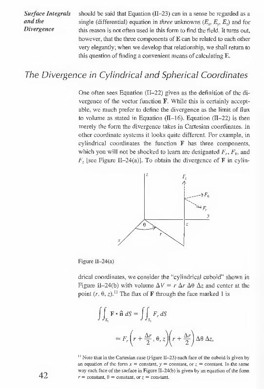
other coordinate systems it looks quite different. For example, in
cylindrical coordinates the function F has three components,
which you will not be shocked to learn are designated Fr, Fe, and
Fz [see Figure II-24(a)]. To obtain the divergence of F in cylin-
42
Figure II-24(a)
drical coordinates, we consider the “cylindrical cuboid” shown in
Figure II-24(b) with volume AV = r Ar A9 Az and center at the
point (r, 0, z).n The flux of F through the face marked 1 is
Jlr'tdS-fl,F'dS (r + ^,e,z)(r + A0 Az,
11 Note that in the Cartesian case (Figure 11-23) each face of the cuboid is given by
an equation of the form x = constant, y = constant, or z = constant. In the same
way each face of the surface in Figure II-24(b) is given by an equation of the form
r = constant, 0 = constant, or z = constant.

The Divergence
in Cylindrical
and Spherical
Coordinates
Figure II-24(b)
while through the face marked 2 it is
dS
Adding these two results and dividing by the volume AV of the
cuboid, we find
Ivl
1
rAr
, Ar r , Ar „ r + ^r Fr r + — ,0, z
2 \ 2
— I r - ^ j F'r (r - , 0, z
which in the limit as Ar (and therefore A V) approaches zero becomes
1 3 , r, jyr(rFr)-
Arguing in an analogous way for the other four faces (see Prob¬
lem 11-18), we arrive finally at the expression for the divergence
in cylindrical coordinates:
div F = Ii_ r dr
1 dFn dF
<rF-)+hi+ii- 43 (11-24)

Surface Integrals
and the
Divergence
Figure 11-25
In spherical coordinates where the components of F are Fr, Fe,
and F,k (see Figure 11-25), similar reasoning (see Problem 11-21)
leads to the expression
div F = \ f (r2Fr) + —r (sin c^F*) + r2 dr r sin <p d<p v
1 dFe r sin <j> 90 '
(11-25)
The Del Notation
There is a special notation in terms of which the divergence may
be written. There would be little or no reason for introducing it if
it served only to provide another way of writing “div,” but as we
shall soon see, it has considerable usefulness in vector calculus.
Let us define a quantity designated V (read “del”) by the fol¬
lowing rather peculiar-looking equation:
V = i_ + jA + dx J dy
k d_
dz '
If we take the dot product of V and some vector function F =
iFx + jFv + kF„ we get
V • F ‘I:+4 + klk(lf‘+jF' + kfJ
= —F dx x
+ A p + A p dy dz Pr
44
Now we interpret the “product” of d/dx and Fx as a partial deriva¬
tive; that is.

The Divergence There are similar equations for the two other “products” (d/dy)Fy
Theorem and (d/dz)Fz. With this convention we recognize V • F (“del dot
F”) as the same as div F, and henceforth, to conform with modem
notational practice, we shall always use V • F to indicate the di¬
vergence. Thus, Equations (11-18) and (11-23) will be written
V • E = p/e0.
Mathematicians call a symbol like V an operator. When we
“operate” with V by dotting it into a vector function, we get the
divergence of that function, as we have just seen. In subsequent
discussions we shall introduce three other quantities (gradient,
curl, and Laplacian), all of which are operators and all of which
can be written in terms of V.
The Divergence Theorem
For the remainder of this chapter we digress from the mainstream
of our narrative to discuss a famous theorem that asserts a re¬
markable connection between surface integrals and volume inte¬
grals. Although this relation may be suggested by the work we
have done in electrostatics, the theorem is a mathematical state¬
ment holding under quite general circumstances. It is independent
of any physics and is applicable in many different places. It is
called the divergence theorem and sometimes Gauss’ theorem
(not to be confused with Gauss’ law).
We shall not give a mathematically rigorous proof of the diver¬
gence theorem; such a proof is given in many texts in advanced
calculus. Instead we present here another physicist’s rough-and-
ready proof. Thus, consider a closed surface S. Subdivide the vol¬
ume V enclosed by S arbitrarily into N subvolumes, one of which
is shown in Figure 11-26 (drawn as a cube for convenience). We
45 Figure 11-26
Surface Integrals
and the
Divergence
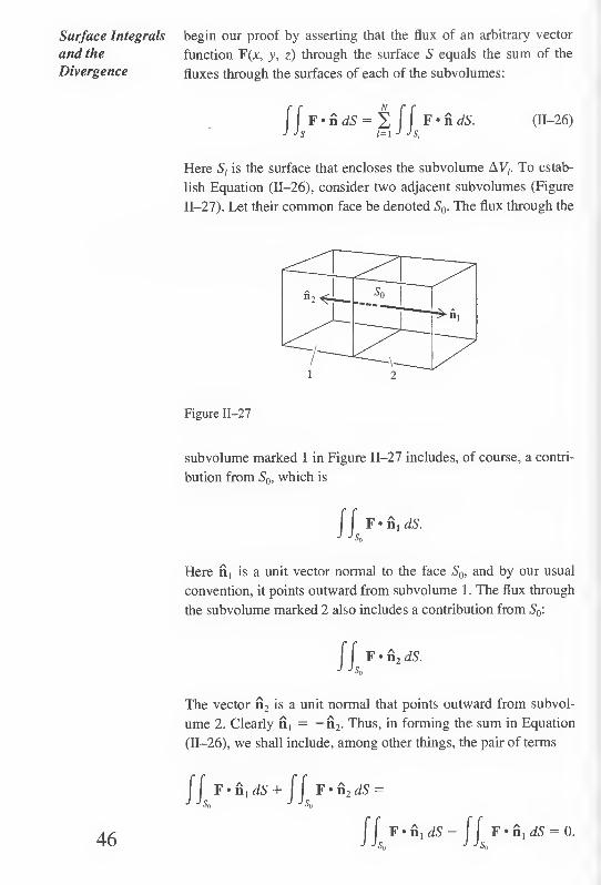
begin our proof by asserting that the flux of an arbitrary vector
function F(x, y, z) through the surface S equals the sum of the
fluxes through the surfaces of each of the sub volumes:
F*n dS £ f f F • n dS. i= 1 J Js,
(11-26)
Here 5, is the surface that encloses the subvolume AV,. To estab¬
lish Equation (11-26), consider two adjacent sub volumes (Figure
11-27). Let their common face be denoted S0. The flux through the
Figure 11-27
subvolume marked 1 in Figure 11-27 includes, of course, a contri¬
bution from S0, which is
F*n {dS.
Here n, is a unit vector normal to the face S0, and by our usual
convention, it points outward from subvolume 1. The flux through
the subvolume marked 2 also includes a contribution from S0:
F • n2 dS.
The vector n2 is a unit normal that points outward from subvol¬
ume 2. Clearly n, = — n2. Thus, in forming the sum in Equation
(11-26), we shall include, among other things, the pair of terms
JJ F*n, dS+ JJ F*n2dS
F • n, dS - F • n, dS = 0. 46

The Divergence
Theorem
We see that these terms cancel each other and there is no net con¬
tribution to the sum in Equation (11-26) due to the face S0. In fact,
this sort of cancellation will obviously occur for any subvolume
surface that is common to two adjacent sub volumes. But all sub¬
volume surfaces are common to two adjacent sub volumes except
those that are part of the original (“outer”) surface S. Hence the
only terms in the sum in Equation (11-26) that survive come from
those subvolume surfaces that, taken together, constitute the sur¬
face S. This establishes the validity of Equation (11-26).
We now rewrite Equation (11-26) in the following curious
fashion:
F*n dS AV, (11-27)
This clearly alters nothing since we have just multiplied and di¬
vided each term of the sum by AV), the subvolume enclosed by the
surface S, We can now imagine partitioning the original volume V
into an ever larger number of smaller and smaller subvolumes. In
other words, we take the limit of the sum in Equation (11-27) as
the number of subdivisions tends to infinity and each AV, tends to
zero. We recognize that the limit of the quantity in square brackets
in Equation (11-27) is, by definition, (V • F);, that is, the divergence
of F evaluated at the point about which A V, is shrinking. Thus, for
each AV, very small. Equation (11-27) becomes
N
F • n dS - 2 (v *F),AV,. /=i
(11-28)
Further, in the limit, this sum is, again by definition, the triple in¬
tegral of V • F over the volume enclosed by S:
lim 2 (V * F), AV, - f f [ V • F dV. (11-29) N-*oo /= i J J Jy
each AV,—>0
Putting together Equations (11-26) through (11-29), we arrive at
our result:
F • n dS = V • F dV. (11-30)
47 This is the divergence theorem. In words, it says that the flux of a
vector function through some closed surface equals the triple inte-

Surface Integrals
and the
Divergence
X s(x„ yi, zi) AV;, i
where the function g is well defined. In Equation (11-27), how¬
ever, the quantity multiplying the volume element AV) in each
term of the sum is not a well-defined function in this sense. That
is, as AV, tends to zero the quantity in the square brackets
changes; it can be identified as the divergence of F only in the
limit. A careful, rigorous treatment would show that Equation
(11-30) is valid if F (that is, F„ Fy, and Fz) is continuous and dif¬
ferentiable, and its first derivatives are continuous in V and on S.
Now let’s illustrate the divergence theorem. Since endless
pages of hideous integrals will not serve our purpose, we’ll use a
simple example. Let
gral of the divergence of that function over the volume enclosed
by the surface.
The major reason the proof given above is not rigorous is that a
triple integral is defined as the limit of a sum of the form
F(x, y, z) = \x + jy + kz
and choose for S the surface shown in Figure 11-28, consisting
of the hemispherical shell of radius 1 and the region R of the
Figure 11-28
xy-plane enclosed by the unit circle. On the hemisphere we have
n = ix + jy + kz, so that n • F = x2+y2 + z2 = 1. Thus, on the
hemisphere,
48 J J F • n dS = J J dS=2Tr,

Two Simple
Applications of
the Divergence
Theorem
where the last equality follows from the fact that the integral is
merely the surface area of the unit hemisphere. On the region R
we have n = —k so that n • F = — z. Hence, on R,
J J F*n dS= -JJ zdxdy = 0
because z = 0 everywhere on R. Thus, there is no contribution to
the surface integral from the circular region R and
F • n dS = 2ir.
Next we find by a trivial calculation that V • F = 3. It follows
then that
where we use the fact that the volume of the unit hemisphere is
2tt/3. Since the surface and volume integrals are equal, this illus¬
trates Equation (11-30).
Two Simple Applications of the Divergence Theorem
As one example of the use of the divergence theorem we give an
alternative derivation of Equation (11-18), the analysis of which
led us to the divergence theorem itself. In other words, this is how
easy it would have been if we had known the divergence theorem
to begin with!
We start with Gauss’ law in the form
jjE-AdS-ljiPdV. (11-31)
Next we apply the divergence theorem to the surface integral in
the above equation to get
ju-ijs-jj'/v- E dV. (11-32)
Thus, combining Equations (11-31) and (11-32), we find
!iirv'EdV=iiilvpdV' 49

Surface Integrals
and the
Divergence
In general, if two volume integrals are equal, it is not necessarily
true that their integrands are equal. It might be that the integrals
are equal only over the particular volume of integration V, and by
integrating over a different volume, we would wreck the equality.
In the present case, however, this is not true because Gauss’ law
holds for any arbitrary volume V, and we cannot upset the equal¬
ity by changing the volume. But this can be so only if the inte¬
grands are equal. Hence,
V • E = p/e0,
which should look familiar!
Another example of the use of the divergence theorem is the
following. Suppose that in some region of space “stuff’ (matter,
electric charge, anything) is moving (Figure 11-29). Let the den-
Figure 11-29
sity of this stuff at any point (x, y, z) and any time t be p(x, y, z, t)
and let its velocity be v(x, y, z, t). Further, suppose this stuff is
conserved; that is, it is neither created nor destroyed. Concentrat¬
ing on some arbitrary volume V in space, we ask: What is the rate
at which the amount of stuff in this volume is changing? At any
time t the amount of stuff in V is
, y, z, t) dV
and the rate at which it is changing is
d_
dt t) dV = dV.
50

Two Simple
Applications of
the Divergence
Theorem
(To be able to move the derivative under the integral sign this
way requires that dp/dr be continuous.)
Next we recall from an earlier discussion that the rate at which
stuff flows through a surface S is
We then assert that the rate at which the amount of stuff in V is
changing is equal to the rate at which it is flowing through the en¬
closing surface 5; in equation form this statement reads
SSSItdv--SSs9"Ads-
There are two features about this equation that require discussion:
1. The negative sign must be included because the surface inte¬
gral as defined is positive for a net flow out of the volume, but
a net flow out means the amount of stuff in the volume is de¬
creasing.
2. This equation states that the amount of stuff in V can change
only as a result of stuff flowing across the boundary S. If stuff
were being created or destroyed in V, terms would have to be
included in the equation to reflect that fact. The absence of any
such terms is thus an expression of the conservation of the
stuff.
Now, finally, let us apply the divergence theorem. We find
• (pv) dV.
Hence,
SiSvtdv’SSIf^>dv- Arguing as we did above that V is an arbitrary volume, we can
then say
51 dp _ = _v . (pv). (11-33)
Surface Integrals
and the
Divergence
Usually we define the current density J = pv and write Equation
(11-31) as
3p
dt + V • J = 0.
An equation of this type is referred to as a continuity equation and
is, as we have seen, an expression of a conservation law (see
Problems III—20, III—21, and IV-21). Besides playing an impor¬
tant role in electromagnetic theory, it is a basic equation both in
hydrodynamics and diffusion theory. Finally, considerations simi¬
lar to those that led to the continuity equation are involved in the
analysis of heat flow.
PROBLEMS
52
II-l Find a unit vector n normal to each of the following surfaces.
(a) z = 2 - x - y. (c) z = (1 - x2)m.
(b) z = (x2 + y2)m. (d) z = x2 + y2.
(e) z = (1 - x2/a2 - y2/a2)wl.
11-2 (a) Show that the unit vector normal to the plane
ax + by + cz = d
is given by
n = ±(i a + j b + k c)/(a2 + b2 + c2)m.
(b) Explain in geometric terms why this expression for n is inde¬
pendent of the constant d.
11-3 Derive expressions for the unit normal vector for surfaces given by
y = g(x, z) and by x = h(y, z). Use each to rederive the expression for
the normal to the plane given in Problem II—2.
IIM In each of the following use Equation 11-12 to evaluate the surface
integral ffs G(x, y, z) dS.
(a) G(x, y, z) = z,
where S is the portion of the plane x + y + z = 1 in the first
octant.
1 + 4(rf + yf where S is the portion of the paraboloid ;
z = 0 and z = 1.
- x2 + y2 betwei
(c) G(x, y, z) = (1 — x2 - y2)312,
where S is the hemisphere z = (1 — x2 — y2)'12.

Problems 11-5 In each of the following use Equation 11-13 to evaluate the surface
integral ffs F • n dS.
(a) F(x, y, z) = ix — kz,
where S is the portion of the plane x + y + 2z = 2 in the first
octant.
(b) F(x, y, z) = ix + jy + kz,
where S is the hemisphere z = Va2 — x2 — y2.
(c) F(x, y, z) = jy + k,
where S is the portion of the paraboloid z — 1 — x2 — y2
above the xy-plane.
11-6 The distribution of mass on the hemispherical shell
z = (fl2 - x2 - y2)1'2
is given by
cr(x, y, z) = (ct0/R2)(x2 + y2)
where cr0 is a constant. Find an expression in terms of <x0 and R for the
total mass of the shell.
II-7 Find the moment of inertia about the z-axis of the hemispherical
shell of Problem II—6.
11-8 An electrostatic field is given by
E = X(iyz + j*z + kxy),
where X is a constant. Use Gauss’ law to find the total charge enclosed
by the surface shown in the figure consisting of Su the hemisphere
z = (R2 — x2 — y2)'12,
and S2, its circular base in the xy-plane.
11-9 An electrostatic field is given by E = X(ix + jy), where X is a con¬
stant. Use Gauss’ law to find the total charge enclosed by the surface
shown in the figure consisting of Slt the curved portion of the half¬
cylinder z = (r2 — y2)l/2 of length h\ S2 and S3, the two semicircular
plane end pieces; and S4, the rectangular portion of the xy-plane. Ex¬
press your results in terms of X, r, and h. 53

Surface Integrals
and the
Divergence
11-10 It sometimes happens that surface integrals can be evaluated with¬
out using the long-winded procedures outlined in the text. Try evaluat¬
ing ffs F • n dS for each of the following; think a bit and avoid a lot
of work!
(a) F = ix + jy + kz.
S, the three squares each of side b as shown in the figure.
(b) F = (ix + jy) ln(x2 + y2).
S, the cylinder (including the top and bottom) of radius R and
height h shown in the figure.
z
54 x
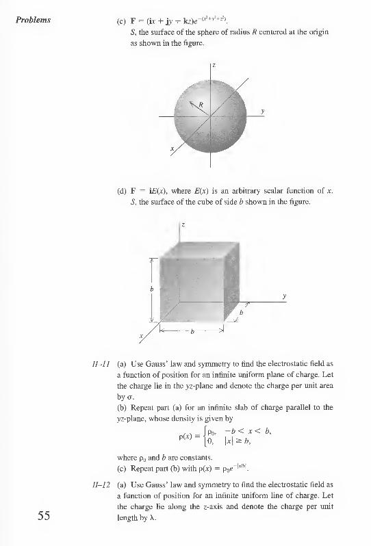
Problems (c) F = (ix + jy + kz)e^+y!+^).
S, the surface of the sphere of radius R centered at the origin
as shown in the figure.
z
y
(d) F = \E(x), where E(x) is an arbitrary scalar function of x.
S, the surface of the cube of side b shown in the figure.
11-11 (a) Use Gauss’ law and symmetry to find the electrostatic field as
a function of position for an infinite uniform plane of charge. Let
the charge lie in the yz-plane and denote the charge per unit area
by cr.
(b) Repeat part (a) for an infinite slab of charge parallel to the
yz-plane, whose density is given by
—b < x < b, \x\ > b.
where p0 and b are constants.
(c) Repeat part (b) with p(x) = p0e
11-12 (a) Use Gauss’ law and symmetry to find the electrostatic field as
a function of position for an infinite uniform line of charge. Let
the charge lie along the z-axis and denote the charge per unit
length by \. 55

(b) Repeat part (a) for an infinite cylinder of charge whose axis
coincides with the z-axis and whose density is given in cylindrical
coordinates by
p(r) = K r<b’ ’ jO, r > b,
where p0 and b are constants.
(c) Repeat part (b) with p(r) = p„e rlh.
11-13 (a) Use Gauss’ law and symmetry to find the electrostatic field as
a function of position for the spherically symmetric charge distri¬
bution whose density is given in spherical coordinates by
P (r) = jpo>
IV
A
?3-
where p0 and b are constants.
(b) Repeat part (a) for p(r) = Po« —rib
(c) Repeat part (a) for
[po. r < b.
P (r) = ■ Pi. b<r<2b.
0, r s 2b.
How must p0 and p, be related so that the field will be zero for
r > 2b? What is the total charge of this distribution under these
circumstances?
11-14 Calculate the divergence of each of the following functions using
Equation (11-22):
(a) ix2 + jy2 + kz2.
(b) iyz + jxz + kxy.
(c) \e~x + \e~y + ke z.
(d) i - 3j + kz2.
(e) (~ixy + j.r)/(x2 + y2), (x, y) * (0, 0).
(f) kVx2 + y2 .
(g) ix + jy + kz._
(h) (-iy + jxl/Vx2 + y2, (x, y) * (0, 0).
11-15 (a) Calculate //5 F • n dS for the function in Problem II-14(a)
over the surface of a cube of side s whose center is at (x0, y0, Zg)
and whose faces are parallel to the coordinate planes.
(b) Divide the above result by the volume of the cube and calcu¬
late the limit of the quotient as s —> 0. Compare your result with
the divergence found in Problem II—14(a).
(c) Repeat parts (a) and (b) for the function of Problem II—14(b)
and (c).
11-16 (a) Calculate the divergence of the function
F(x, y, z) = if(x) + j/(y) + k/(-2z)
56 and show that it is zero at the point (c, c, —cl2).
Surface Integrals
and the
Divergence

Problems (b) Calculate the divergence of
G(r, y, z) = i/Cy, z) + jg(x, z) + kh(x, y).
11-1 7 In the text we obtained the result
V • F = dFx dFy
dx ay dJl dz
by integrating over the surface of a small rectangular parallelepiped.
As an example of the fact that this result is independent of the surface,
rederive it using the wedge-shaped surface shown in the figure.
11-18 (a) Let i, j, and k be unit vectors in Cartesian coordinates and er,
e0, and e, be unit vectors in cylindrical coordinates. Show that
i - er cos 0 — e0 sin 0,
j = er sin 0 + ee cos 0 ,
k = e,.
(b) Rewrite the function in Problem II-14(e) in cylindrical coor¬
dinates and compute its divergence, using Equation (11-24). Con¬
vert your result back to Cartesian coordinates and compare with
the answer obtained in Problem II—14(e).
(c) Repeat part (b) for the function of Problem II-14(f).
11-19 (a) Let i, j, and k be unit vectors in Cartesian coordinates and er,
e0, and e* be unit vectors in spherical coordinates. Show that
i = er sin 4> cos 0 + e4 cos 4> cos 0 — ee sin 0
j = er sin <j> sin 0 + cos 4> sin 0 + e0 cos 0
k = er cos <(> - sin 4>
[Hint: It’s easier to express er, e0, and e* in terms of i, j, and k
and then solve algebraically for i, j, and k. To do this, first use the
fact that er = rlr = (vc + jy + kz)/r. Next, reasoning geometri¬
cally, show that e0 = — i sin 0 + j cos 0. Finally, calculate e4, =
e0 X er.]
(b) Rewrite the function of Problem II—14(g) in spherical coordi¬
nates and compute its divergence using Equation (11-25). Convert 57

Surface Integrals
and the
Divergence
your result back to Cartesian coordinates and compare with the
answer obtained in Problem II—14(g).
(c) Repeat part (b) for the function of Problem II—14(h).
11-20 In cylindrical coordinates the divergence of F is given by
. F = - — (rF ) + - — r dr y r> r 30
dF, dz
In the text (pages 42-43) we derived the first term of this expression.
Proceeding the same way, obtain the other two terms.
11-21 Repeat Problem 11-20 to obtain the divergence in spherical coordi¬
nates by carrying out the surface integral over the surface of the vol¬
ume shown in the figure and thereby obtaining the expression
V • F = -y (r2Fr) + —(sin (J> FA + r2 dr r sin 4> d<t> ^
1 dFfi
r sin 4> 50
11-22 Consider a vector function of the form
F(r) = er/(r),
where er = (ix + jy + kz)/r is the unit vector in the radial direction,
r = (x2 + y2 + z2)u2, and f(r) is a differentiable scalar function. Using
the results of Problem 11-21, determine/(r) so that V • F = 0. A vector
function whose divergence is zero is said to be solenoidal.
11-23 Verify the divergence theorem
/£F-fias = //J V-FdV
in each of the following cases:
(a) F = ix + jy + kz.
S, the surface of the cube of side b shown in the figure. 58

Problems
(b) F = V + ezz,
r = ix + jy. S, the surface of the quarter cylinder (radius R, height h)
shown in the figure.
(c) F = er r2,
r = ix + jy + kz.
S, the surface of the sphere of radius R centered at the origin
as shown in the figure.
59

Surface Integrals
and the
Divergence
for any closed surface S.
(b) Determine the flux of a uniform magnetic field B through the
curved surface of a right circular cone (radius R, height h) ori¬
ented so that B is normal to the base of the cone as shown in the
figure. (A uniform field is one that has the same magnitude and
direction everywhere.)
11-24 (a) One of Maxwell’s equations states that V • B = 0, where B is
any magnetic field. Show that
II, B • n dS = 0
11-25 Use the divergence theorem to show that
JJ ndS = 0,
where S is a closed surface and n is the unit vector normal to the
surface S.
11-26 (a) Use the divergence theorem to show that
Ws^rds=v’
where S' is a closed surface enclosing a region of volume V, n is a
unit vector normal to the surface S, and r = ix + jy + kz.
(b) Use the expression given in (a) to find the volume of
(i) a rectangular parallelepiped with sides a, b, c.
(ii) a right circular cone with height h and base radius R.
[Hint: The calculation is very simple with the cone ori¬
ented as shown in the figure.]
(iii) a sphere of radius R. 60

Problems
11-27 (a) Consider a vector function with the property V • F = 0
everywhere on two closed surfaces S, and S2 and in the volume V
enclosed by them (see the figure). Show that the flux of F
through S, equals the flux of F through S2- In calculating the
fluxes, choose the direction of the normals as indicated by the ar¬
rows in the figure.
(b) Given the electrostatic field of a point charge q situated at
r = 0,
where r2 = x2 + y2 + z2, show by direct calculation that
V • E = 0, for all r + 0.
(c) Prove Gauss’ law for the field of a single point charge given
in (b). [Hint: It is easy to calculate the flux of E over a sphere
centered at r = 0.]
(d) How would you extend this proof to cover the case of an ar¬
bitrary charge distribution? 61

Surface Integrals
and the
Divergence
11-28 (a) Show by direct calculation that the divergence theorem does
not hold for /\.
F(r,e. 4>) = -^, rl
with S the surface of a sphere of radius R centered at the origin,
and V the enclosed volume. Why does the theorem fail?
(b) Verify by direct calculation that the divergence theorem does
hold for the function F of part (a) when S is the surface S, of a
sphere of radius Rt plus the surface ,S'2 of a sphere of radius R2,
both centered at the origin, and V is the volume enclosed by S{
and S2.
(c) In general, what restriction must be placed on a surface S' so
that the divergence theorem will hold for the function of part (a)?
62

Chapter III
Line Integrals and the Curl
To err from the right path is common to Mankind.
Sophocles
Work and Line Integrals
We remarked above that the differential form of Gauss’ law,
Equations (11-18) and (11-23), although it fulfills our goal of relat¬
ing a property of the electric field (its divergence) at a point to a
known quantity (the charge density) at the same point, nonethe¬
less falls short of providing a convenient way to find E. The rea¬
son is that V • E = p/e0 is (or seems to be) a single differential
equation in three unknowns (E„ Ey, £..). But there is another fea¬
ture of electrostatic fields that has not yet played an explicit role
in our discussion and that will yield a relationship among the
components of E. It will thus provide us with the crucial last step
in obtaining a useful way to calculate fields. In the process of ex- 63

Line Integrals
and the Curl
amining this question, we shall encounter some of the most im¬
portant topics in vector calculus.
The property of electrostatic fields that we shall now begin to
discuss is intimately bound up with the question of work and en¬
ergy. You no doubt recall the elementary definition of work as
force times distance. Thus, in one dimension, if a force F(x) acts
from x = a to x = b, the work done is, by definition,
[ F(x) dx.
To be able to handle more general situations, we must now intro¬
duce the concept of the line integral.
Figure III—1
Suppose we have a curve C in three dimensions (Figure III—1)
and suppose the curve is directed. By this we mean that we put an
arrow on the curve and say “This is the positive direction.” Let s
be the arc length measured along the curve from some arbitrary
point on it with s = s, at a point P] and s = .5, at P2. Suppose fur¬
ther that we have a function f(x, y, z) defined everywhere on C.
Now let us subdivide the portion of C between P, and P2 arbitrar¬
ily into N sections. Figure III—1 shows an example of such a sub¬
division for N = 4. Next, join successive subdivision points by
chords, a typical one of which, say the Zth, has length As,. Now
evaluate/(x, y, z) at (xh yb z.t), which is any point on the Zth subdi¬
vision of the curve, and form the product/(jc,, y,, z,) As,. Doing
this for each of the N segments of C, we form the sum
N
E /(*/> ybZi)As,. 1= 1
64

Work and Line
Integrals
By definition, the line integral of fix, y, z) along the curve C is the
limit of this sum as the number of subdivisions N approaches in¬
finity and the length of each chord approaches zero:
L fix, y, z) ds = lim % fix,, y„ z,) A s,. N—> 00 /= 1
each As —*0
To evaluate the line integral, we need to know the path C. Usu¬
ally the most convenient way to specify this path is parametrically
in terms of the arc length parameter s. Thus, we write x = x(s),
y — y(s), and z = z(s). In such a situation the line integral can be
reduced to an ordinary definite integral:
J f(x, y, z)ds = J f[x(s), y(s), z(s)] ds.
An example of a line integral will be helpful here. For simplic¬
ity let us work in two dimensions and evaluate
J (x + y) ds,
where C is the straight line from the origin to the point whose co¬
ordinates are (1, 1) (Figure III—2). If (x, y) are the coordinates of
Figure III—2
any point P on C and if s is the arc length measured from the ori¬
gin, then x = 5/V2 and y = .s/V2. Hence, x + y = 2s/V2 =
V2s. Thus,
65 s ds = V2.

Line Integrals
and the Curl (l, l)
A c2
c, x
Figure III—3
Let us integrate this same function (x + y) from (0, 0) to (1, 1)
along another path as shown in Figure III—3. Here we break the
integration into two parts, one along C, and the second along C2.
On C] we have x = s and y = 0. Thus, on C1( x + y = s, and so
J (x + y) ds — J sds = 5.
Along C2, x = 1 and y = s [note that the arc length on this seg¬
ment of the path is measured from the point (1, 0)]. It follows
then that
Adding the results for the two segments, we find
[ (x + y)ds = [ (x + y)ds + f (x + y) ds = { + | = 2. Jc Jcl Jc2
The lesson to be learned is this: the value of a line integral can
(indeed, usually does) depend on the path of integration.
Line Integrals Involving Vector Functions
Although the preceding discussion tells us what a line integral is,
the kind of line integral we must deal with here has a feature not
yet mentioned. You will recall that we introduced our discussion
of line integrals with the concept of work. Work, in the most ele-
66

Line Integrals
Involving Vector
Functions
mentary sense, is force times displacement. That this needs elabo¬
ration becomes clear when we recognize that both force and dis¬
placement are vectors.
Thus, consider some path C in three dimensions (Figure III—4).
Let us suppose that under the action of a force an object moves on
this path from 5, to s2. At any point P on the curve let the force
Figure III—4
acting be designated f(x, y, z). The component of f that does work
is, by definition, only that one which acts along the curve, that is,
the tangential component. Let t denote a unit vector that is tan¬
gent to the curve at P} Then the work done by the force in mov¬
ing the object from s, to s2 along the curve C is
where it is understood, of course, that the integration begins at
s = 5, and ends at s = s2. The new feature of this integral is that
the integrand is the dot product of two vector functions. To be A
able to handle such a line integral, we must know how to find t,
and it is to this problem that we now turn.
Consider an arbitrary curve C (Figure III—5) parametrized by
its arc length. At some point s on the curve we have x = x(s), y =
y(s), and z = z(s). At another point s' + As we have x + Ax =
x(s + As), y + Ay = y(s + As), and z + Az = z(s + As). Thus,
1 t is a function of x, y, and z and should really be written t (x, y, z). We write sim¬
ply t to avoid complicating the notation.
67

Line Integrals
and the Curl
Figure III—5
the chord joining the two points on the curve directed from the
first to the second is the vector Ar = iAx + jAy + kAz, where
Ax = x(s + As) — x(s),
Ay = y(s + As) - y(s),
A z = z(s + As) — z(s).
If we now divide this vector by As, we get
Ar
As + k
Az
As'
Taking the limit of this as As approaches zero yields
idx , .dy dz
ds J ds ds’
/v
and we assert that this is t. To begin with, it’s clear that as As —» 0,
the vector Ar becomes tangent to the curve at s. Further, in the limit
As —» 0, we see that |Ar| —> As. Hence, in the limit the magnitude of
this quantity is 1. It follows then that we can make the identification
/>, . . dx , .dy dz t(s) = i— + i — + k —.
ds J ds ds
If we return now to the expression for work W and use this for- A
mula for t, we find
W . dx , -^y + kdz
1 ds ^ ds ds = [ f(x, y, z)
J c
= J (fxdx +fydy +fzdz).
ds
68

Line Integrals
Involving Vector
Functions
This is a formal expression; often, to carry out the integration, it
is useful to restore the ds as the following example illustrates.
Consider
f(x, y, z) = iy - jx
and the path shown in Figure III-6(a). To calculate fc(f • t) ds in
Figure III—6(a)
this case, we break the path C into three parts, Ch C2, and C3 as
shown. Since fz = 0, we have
j" f • *ds = Ic ^dx+^>dy
— I y dx — xdy. J c
Now, on C,, y — 0 and dy = 0, so there is no contribution to the
integral. Similarly, on C3 we have x = 0 and dx = 0, and again
the result is zero. Thus, the only contribution to the integral over
C can come from C2. Restoring the ds, we have
69

Line Integrals
and the Curl
Figure III-6(b)
But (1 — x)/s = cos 45° = 1/V2 and y/s = sin 45° = 1/V2
[Figure III—6(b)]. Thus,
_ , _ s dx 1_
X V2 ds V2
5 dy _ 1
y V2 ds y/2
0 < s < V2.
Hence, the integral is
1
V2 ds — — 1.
As a second example of a line integral involving a vector func¬
tion, let
f(x, y, z) = ix2 - jxy,
and take C to be the quarter circle of radius R oriented as shown
in Figure III-6(c). We then have
f'tds= x2 dx — xy dy. J c J c
70

Path
Independence
Figure III-6(c)
Letting x = R cos 0, y = R sin 0, we find this integral becomes
r-ir/2
j 0
[/?2 cos2 Q(-R sin 0) - R2 sin 0 cos 0(7? cos 0)] <70
= -2R? rn/2
j 0 cos2 0 sin 0 dO = — 2f?3/3.
Path Independence
In a line integral the path of integration is one of the ingredients
which determines the very function we integrate. It isn’t remark¬
able, then, that the value of the integral can depend on the path of
integration. What is remarkable is that, under some conditions,
the value of the integral does not depend on the path!
We show how this path independence comes about in the case
of the Coulomb force. Let a charge q0 be fixed at the origin and
let another charge q be situated at (x, y, z) (Figure III—7). The
Coulomb force on q is
F = l qqo
4tt€0 r2
/V
U, (in—i)
71
where r = (x2 + y2 + z2)172 is the distance between the two
charges and u is a unit vector pointing from q0 to q. With this
arrangement u is clearly in the radial direction. Even more

Line Integrals
and the Curl
Figure III—7
clearly, the radial vector r is in the radial direction. Thus, we have
u = r/r = (ix + jy + kz)/r, and so
F _ Wo i^ + jy + kz
4-ireo r3
Thus,
F• t ds = Fx dx + Fy dy + Fz dz = qq0 xdx + y dy + zdz
4'rre0 r3
The trick now is to use the relationship
r2 = jc2 + y2 + z2.
Taking differentials in this equation and dividing by a factor of 2
yields
xdx + y dy + zdz = r dr.
so that
c, £ j _ Wo r dr Wo dr b • t ds = --r— = ---.
4tt€0 r3 4-ireo r2
Suppose now that the charge q moves from a point P, at a dis¬
tance r, from the origin to a point P2 at a distance r2, over some
path C connecting the two points (Figure III—8). Then
/, F A
t ds = Wo fr* dr
4Tre0Jr| r2 Wo /1
4lTe0 \ri 72

Path
Independence
Figure III—8
Notice that to get this result, we haven’t had to specify C in any
way whatever; we’d get the same answer for any path connecting
P, and P2. This, of course, proves that the line integral
f F*t ds J c
with F given by Equation (III—1) is path-independent, but the re¬
sult, so far, has been established only for the Coulomb force on q
due to a single charge q{) [Equation (III—1)]. If there are many
charges qu q2,, qN, then the total force on is F, + F2 +
■ ■ • + ¥n, where F; is the Coulomb force on q due to the /th
charge q,. Hence,
J F • t ds = J F, • t ds 4-K J Fn • t ds.
Now the discussion given above shows that each term of this sum
is path independent; hence, so is the sum itself. (All this, of
course, is merely an application of the superposition principle.)
To phrase this result in terms of the field requires one last trivial
step: Since F = qE, it follows that q Jc E • t ds is path indepen¬
dent, whence /CE • t ds is also. Strange to say, it is this fact that
will enable us eventually to convert V • E = p/e0 into a more use¬
ful equation.
If you examine the foregoing discussion carefully, you’ll see
that the fact that the Coulomb force varies inversely as the square
of r has nothing whatever to do with the path independence of the
line integral. The path independence rests solely on two proper¬
ties of the Coulomb force: (1) It depends only on the distance be¬
tween the two particles, and (2) it acts along the line joining them. 73

Line Integrals
and the Curl
Any force F with these two properties is called a central force,
and fc F • t ds is independent of path for any central force.2
One further step pertaining to path independence can be taken
here. If
L F • t ds
is independent of path, then
I F • t ds= F • t ds, Jc, Jc1
where, as indicated in Figure III—9, C, and C2 are two different ar¬
bitrary paths connecting the two points P, and P2 and directed as
shown in the figure. Now if instead of integrating along from
P, to P2, we go the other way, we simply change the sign of the
line integral; that is,
F • t ds F • t ds.
Figure HI-9
where -C, merely indicates that the integration is to be carried
out along C, from P2 to P,. Thus,
F • t ds = F • t ds
2 Our having illustrated path independence with a central force may give the erro¬
neous impression that only central forces have path-independent line integrals.
That is certainly not true; many functions which are not central forces have path-
independent line integrals. Later we’ll develop a simple criterion for identifying
such functions. 74
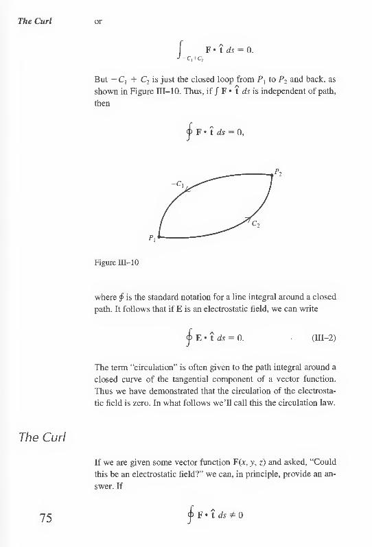
The Curl or
t ds = 0.
But — C, + C2 is just the closed loop from P] to P2 and back, as
shown in Figure III—10. Thus, if / F • t ds is independent of path,
then
F • t ds = 0,
Figure III-10
where $ is the standard notation for a line integral around a closed
path. It follows that if E is an electrostatic field, we can write
f E • t ds = 0. (Ill—2)
The term “circulation” is often given to the path integral around a
closed curve of the tangential component of a vector function.
Thus we have demonstrated that the circulation of the electrosta¬
tic field is zero. In what follows we’ll call this the circulation law.
The Curl
75
If we are given some vector function F(x, y, z) and asked, “Could
this be an electrostatic field?” we can, in principle, provide an an¬
swer. If

Line Integrals
and the Curl
over even one path, then F cannot be an electrostatic field. If
F • t ds = 0
over every closed path, then F can (but does not have to) be an
electrostatic field.
Clearly, this criterion is not easy to apply since we must be sure
the circulation of F is zero over all possible paths. To develop a
more useful criterion, we proceed much as we did in dealing with
Gauss’ law, which, like the circulation law, is an expression involv¬
ing an integral over the electric field. Gauss’ law is more useful in
the differential form [Equations (11-18) and (11-23)] obtained by
considering the ratio of flux to volume for ever-decreasing sur¬
faces. We now treat the circulation law in the same spirit and at¬
tempt to find the differential form of Equation (III—2). To stress
the generality of our analysis and results, we deal with an arbi¬
trary function F(x, y, z) and specialize to E(x, y, z) at a later stage
in the development.
Let us consider the circulation of F over a small rectangle par¬
allel to the xy-plane, with sides Ax and Ay and with the point
(x, y, z) at the center [Figure III-11(a)]. As shown in Figure
III-11(b), we carry out the path integration in a counterclockwise
direction looking down at the xy-plane. The line integral is broken
up into four parts: CB (bottom), CK (right), CT (top), and CL (left).
Since the rectangle is small (eventually we shall take the limit as
it shrinks down to zero), we’ll approximate the integral over each A
segment by F • t evaluated at the center of the segment, multi¬
plied by the length of the segment.3
Figure H[-l 1(a)
76 3 Reread footnote 9 of Chapter n and then give an argument in support of this
approximation.
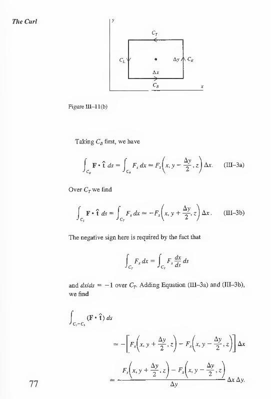
The Curl y
cT
cB
Figure m-l 1(b)
Taking CB first, we have
J F • t ds = J Fxdx — Fx(^c,y —^, z j Ax. (III-3a)
Over CT we find
J F-t ds = J Fxdx — ~Fx^x, y + zj Ax. (Ill—3b)
The negative sign here is required by the fact that
and dx/ds = -1 over CT. Adding Equation (III—3a) and (III—3b),
we find

Line Integrals
and the Curl
The factor Ax Ay is clearly the area AS of the rectangle. Thus,
X A S
(F • t) ds (HI—4)
— Fr Ay
2
Ay
Exactly the same sort of analysis applied to the left and right sides
of the rectangle (CL and CR) results in
x AS
(F • t) ds
Fv x + Ax
,y,z Fv * ~ - y. z Ay 2
Ax (HI—5)
Adding Equations (III^l) and (III—5) and taking the limit as AS
shrinks down about a point (x, y, z) (in which case Ax and Ay —» 0
as well), we get
lim -L [£ AS—>0 J
about (x,_y,2)
/v dF F • t ds =
uX
dFx dy ’
(HI—6)
where $ is our semicomical notation meaning the circulation
around the little rectangle.
You may wonder about the generality and uniqueness of this
result since it is obtained using a path of integration that is spe¬
cial in two ways: first, it is a rectangle, and second, it is parallel
to the xy-plane. If the path were not a rectangle, but a plane
curve of arbitrary shape, it would not affect our result (see
Problems III—2 and III—30). But our result definitely does de¬
pend on the special orientation of the path of integration. The
choice of orientation made above clearly suggests two others,
and they are shown in Figure III-12(a) and (b) along with the
result of calculating
lim ~ [D F • t ds AS-^O A S T
about (x,y,z)
78 for each.

The Curl
Figure III-12(a)
Figure III-12(b)
Each of these three paths is named in honor of the vector nor¬
mal to the enclosed area. The convention we use is this: Trace the
curve C so that the enclosed area is always to the left [Figure
III—13(a)]. Then choose the normal so that it points “up” in the di-
79 Figure III—13(a)

Line Integrals
and the Curl
n
Figure III—13(b)
rection shown in the picture. This convention is sometimes called
the right-hand rule, for if the right hand is oriented so that the fin¬
gers curl in the direction in which the curve is traced, the thumb,
extended, points in the direction of the normal [Figure III—13(b)].
Using the right-hand rule, we have the following:
Calculating limM^0 § F • t ds/AS
for a path whose normal is i, we get
for a path whose normal is j, we get
for a path whose normal is k, we get
dIi dy
dF*
dz
dFy
dx
dFy '
dz ’
dh ■ dx ’
dl± dy '.
(Ill—7 a)
It turns out that these three quantities are the Cartesian compo¬
nents of a vector. To this vector we give the name “curl of F,”
which we write curl F. Thus, we have
curl F = i dz J J\dz dx)
+ k (III—7b)
80
This expression is often (indeed, usually) given as the definition
of the curl, but we prefer to regard it as merely the form of the
curl in Cartesian coordinates. We shall define the curl as the limit

The Curl z
Figure III-14
of circulation to area as the area tends to zero. To be precise, let
<fcF • t ds be the circulation of F about some path whose normal
is n as shown in Figure III—14. Then by definition
n • curl F = lim F • t ds. (III-8) AS—»o Ao J cn
about (x,y,z)
By taking n successively equal to i, j, and k, we get back the results
given in Equation (III—7b). Since this limit will, in general, have dif¬
ferent values for different points (x, y, z), the curl of F is a vector
function of position.4 Note incidentally that although in our work we
always assumed that the area enclosed by the path of integration was
a plane, this need not be the case. Since the curl is defined in terms
of a limit in which the enclosed surface shrinks to zero about some
point, in the final stages of this limiting process the enclosed surface
is infinitesimally close to a plane, and all our considerations apply.
Since it is undoubtedly beyond the powers of a mere mortal to
remember the expression given above for curl F in Cartesian coor¬
dinates [Equation (III—7b)], it is fortunate that there is a mnemonic
device to fall back on. If the three-by-three determinant
i j k
d/dx d/dy d/dz
Fx Fy F-
is expanded (most conveniently in minors of the first row) and if
certain “products” are interpreted as partial derivatives [for example,
81
4 The word rotation (abbreviated “rot,” amusingly enough) was once used for
what we now call the curl. Though the term has long since dropped out of use, a
related one survives: If curl F = 0, the function F is said to be irrotational.

Line Integrals
and the Curl (d/dx)Fy = dFy/dx], the result will be identical with the one given in
Equation (III—7b).5 Thus, the anguish of remembering the form of
curl F in Cartesian coordinates can be replaced by the pain of re¬
membering how to expand a three-by-three determinant. Chacun a
son gout.
As an example of calculating the curl, consider the vector
function
F(x, y, z) = ixz + jyz ~ ky2.
We have
curl F =
i J k
d/dx d/dy d/dz
xz yz ~y
= i(—2y -y)+ j(x - 0) + k(0 - 0)
= -3iy + jx.
You may have noticed that the curl operator can be written in
terms of the del notation we introduced earlier. You can verify for
yourself that
curl F = V X F,
which is read “del cross F.” Henceforth, we shall always use
V X F to indicate the curl.
The Curl in Cylindrical and Spherical Coordinates
To obtain the form of V X F in other coordinate systems, we pro¬
ceed as we did above in finding the Cartesian form, merely modi¬
fying the paths of integration appropriately. As an example, using
the path shown in Figure III—15(a) will yield the ^-component of
V X F in cylindrical coordinates.6 Note that we trace the curve in
82
5 A mathematician would object to this since, strictly speaking, a determinant can¬
not contain either vectors or operators. We aren’t doing any serious damage, how¬
ever, because our “determinant” is merely a memory aid.
6 In deriving the Cartesian form of V X F, each segment of each path of integra¬
tion (see Figures HI-11 and IH-12) was of the form x = constant, y = constant, or
Z = constant. Similarly, in deriving the cylindrical form, each segment of each
path is of the form r = constant, 0 = constant, or z = constant.

z The Curl in
Cylindrical and
Spherical
Coordinates
Figure III-15 (a)
x
Figure III-15(b)
accordance with the right-hand rule given in the previous section.
Viewing the path from above [as we do in Figure III—15(b)], the
line integral of F(r, 0, z) • t along the segment of path marked 1 is
J F* t ds^Fr(r,Q — ^r>z) Ar,
while along segment 3 it is
f F • t ds = -Fr ^r, 6 + y-, zj Ar.
The area enclosed by the path is r Ar A0, so

Line Integrals
and the Curl In the limit as Ar and A0 tend to zero, this becomes
_\dFr
r 50
evaluated at the point (r, 0, z).
Along segment 2 we find
F.(r + f,e,z)(r + f)48.
and along segment 4
Thus,
_L AS I J C,+C4
F• t ds — A0
r Ar A0
In the limit this becomes (l/r)(5/5r)(rFe) evaluated at (r, 0, z).
Hence,
(V X F), lim — as—>o AS
F • t ds = ~ ~ (rFe) - r 50 '
Paths for finding the r- and 0-components of V X F are shown in
Figures III—15(c) and (d), respectively. You are asked to obtain
these two components yourself in Problem III—8. For com¬
pleteness we give all three components of V X F in cylindrical
coordinates:
„ 1 5F. (VXF) = - —- ( ,r r ae
(VXF),»f-
5Fe
5z ’
BF.
dr ’
(VxF); = ^frFfl)- 1 9Fr
r 50 ‘ 84

z The Curl in
Cylindrical and
Spherical
Coordinates
Figure III-15(c)
Figure III-15(d)
As an example of calculating the curl in cylindrical coordinates
consider the function
F(r, 0, z) = err2z + eerz2 cos 0 + ezr3
Then
(VXF)r=p^ (r3) - (rz2 cos 0) = -2rz cos 0
(VXF)s = ^(r2z)-|(r3)= -2r2
(VXF); = }|; (r2z2 cos 0) - j ^ (r2z) = 2z2 cos 0
Hence
85 V X F = -2errz cos 0 - 2ee r2 + 2ez z2 cos 0

Line Integrals The three components of curl F in spherical coordinates (see
and the Curl Problem III—9) are as follows:
(V X F)r 1
r sin <}> 3<j> d (sin <f> Fe) - 1
3F*
r sin 4> 30
(VxF)* = 7^^-i£(rFe) r sin <J) 30 r dr
As an example of calculating the curl in spherical coordinates,
consider the function
TJY A i \ _ ^ r j F(r, 0, 4>) ~ + ~T +
r 0 r r cos cj>
Then
(V X F)r = sin 4> sec2 <|>
r sin 4> 34> \ r cos 4>/ r sin <j) r2 sin 4>
(V X F)* = 1 3/1 1 3
-77=(C0S <!>) = 1
r sin <)) 30 \r0/ r dr
(V X F)e = ~ ~~ (1) “ 9 1 1 3<() \r 0
r202 sin 4>
= 0
Hence
V X F = sec2 <j> ^ —r-e r sin ()>
1
r202 sin c()
A
The Meaning of the Curl
The preceding discussion may leave you with the feeling that
knowing how to define and calculate the curl of some vector func¬
tion is a far cry from knowing what it is. The fact that the curl has
something to do with a line integral around a closed path (indeed,
the word “curl” itself) may suggest to you that it somehow has to
do with things rotating, swirling, or curling around. By means of
a few examples taken from fluid motion, we’ll try to make these
vague impressions a little clearer. 86

The Meaning of
the Curl
87
Figure III-16
Suppose water is flowing in circular paths, something like the
water draining from a bathtub. A small volume of the water at a
point (x, y) at time t has coordinates x = r cos lot, y = r sin cot,
where co is the constant angular velocity of the water (Figure
III-16).7 Thus, its velocity at (x, y) is
v = i(dx/dt) + j(dy/dt) = rco[—i sin cot + j cos cot]
= co(-iy + j*).
This expression gives what is called the velocity field of the
water; it tells us the velocity of the water at any point (x, y). Your
intuition probably tells you that, because the motion is circular,
this velocity must have a nonzero curl. In fact, as you can show
very easily.
V X v = 2kco.
This result should seem quite reasonable because it says that curl of
the velocity is proportional to the angular velocity of the swirling
water. We see that V X v is a vector perpendicular to the plane of
motion and in the positive z-direction [Figure III—17(a)]. If the
water were rotating around in the other direction, the curl of v
would then be in the negative z-direction [Figure ni-17(b)]. Note
that this is consistent with the right-hand rule (see page 79-80). If
7 This is not a realistic description of water draining from a tub since rotating
water shears tangentially and its angular velocity will therefore vary with r. The
crude description we use here is adequate for our purposes and has the virtue of
being simple.

Line Integrals
and the Curl
Figure III—17(a)
Figure III-17(b)
we were to put a small paddle wheel in the water, it would com¬
mence spinning because the impinging water would exert a net
torque on the paddles (Figure III—18). Furthermore, the paddle
wheel would rotate with its axis pointing in the direction of the curl.
Figure III-18
Now consider a different velocity field, namely,
v = jv0e~y2/^, 88

The Meaning of
the Curl
Figure III-19
where v0 and X are constants. Water with such a velocity field
would have a flow pattern as indicated in Figure III—19. The ve¬
locity at all points is in the positive y-direction, and its magnitude
(indicated by the length of the arrows) varies with y. Since you
see only straight line flow here without any rotational motion, you
would probably guess that V X v = 0 in this case, and you would
be right, as a simple calculation shows. There would be no net
torque on a paddle wheel placed anywhere in this flow pattern,
and as a consequence, it would not spin.8
Our last example is trickier than the two given previously and
shows that intuition can lead you astray if you’re not careful. Let
a velocity field be given by
v = jv0e x,k\
As in the previous example, the velocity in this case is every¬
where in the y-direction, but now it varies with x, not y (Figure
III—20). Here, as in the preceding example, you see no evidence
of rotational motion and you might guess that V X v = 0 once
again. But as you should show for yourself,
V X v = -ku0 H e~xW. X2
A small paddle wheel placed in this flow pattern would spin, even
though the water is everywhere moving in the same direction. The
89 If V X v = 0, the flow is said to be irrotational. Compare with footnote 4.

Line Integrals
and the Curl
Figure III—20
reason this happens is that the velocity of the water varies with x,
so that it strikes one of the paddles (P in Figure III—21) with
greater velocity than the other (P'). Thus, there will be a net
torque. In more mathematical terms, the line integral of v • t
around a small rectangle (Figure III—22) will be different from
zero, for while
vtds = v • t ds = 0, ^ bottom J top
the contributions from the other two sides are
/ ■ J right
v • t ds — vy(x + Ax) Ay
90 Figure III-21

Differential Form of the Circulation Law
y
Figure III—22
and
v • t ds — —vy (x) Ay.
These do not cancel because vy(x) # vy(x + Ax). Incidentally,
you should try to explain to your own satisfaction why in this ex¬
ample V X v is in the negative (positive) z-direction when x is
positive (negative) and why VXv = 0atJC = 0.
Differential Form of the Circulation Law
The curl is defined to be the limit of circulation to area. Thus,
n • V X E = lim <f> E • t ds, as-*o AS J c
where n is a unit vector normal to the surface enclosed by C at the
point about which the curve shrinks to zero. But if E is an electro¬
static field, then
E • t ds 0
for any path C. It follows that
91 n • V X E = 0.

Line Integrals
and the Curl Since the curve C is arbitrary, we can arrange matters so that n is
a unit vector pointing in any direction we choose. Thus,
taking n = i, we have (V X E)* = 0;
taking n = j, we have (V X E)y = 0;
taking n = k, we have (V X E)z = 0.
Thus, all three Cartesian components of V X E vanish, and we
can conclude that for an electrostatic field,
V X E = 0.
This is the long-sought-after differential form of the circulation
law. We are now in a position to give an alternative and much
more tractable answer to the question “Can a given vector func¬
tion F(x, y, z) be an electrostatic field?” The answer is
IfV X F = 0, then F can be an electrostatic field, and
if V X F # 0, then F cannot be an electrostatic field.
This is clearly a much more convenient criterion to apply than our
earlier one (page 77), which required us to determine the line in¬
tegral of F over all closed paths! To see how it works, let us do
several examples.
Example 1. Could F = K(iy + jx) be an electrostatic field? (K
is a constant.) Here we have
±VXF
9y\ dyj
= 0=>VXF = 0.
Answer: Yes.
Example 2. Could F = K(iy — jx) be an electrostatic field? In
this case
ivxF = dy\
By) —2k => V X F = -2kK.
92 Answer: No.

Stokes’ Theorem From these examples we can see how easy this criterion is to
apply.
Stokes' Theorem
For the remainder of this chapter we digress from our presenta¬
tion to discuss another famous theorem, one strongly reminiscent
of the divergence theorem and yet, as we’ll see, quite different
from it. This theorem, named for the mathematician Stokes, re¬
lates a line integral around a closed path to a surface integral over
what is called a capping surface of the path, so the first item on
our agenda is to define this term. Suppose we have a closed curve
C, as shown in Figure III—23(a), and imagine that it is made of
Figure III—23(a)
wire. Now let us suppose we attach an elastic membrane to the
wire as indicated in Figure III—23(b). This membrane is a capping
Figure III-23(b)
surface of the curve C. Any other surface which can be formed by
stretching the membrane is also a capping surface; an example is
shown in Figure III—23(c). Figure III—24 shows four different
capping surfaces of a plane circular path: (a) the region of the
93 Figure III—23(c)

Line Integrals
and the Curl
Figure HI-24
plane enclosed by the circle, (b) a hemisphere with the circle as
its rim, (c) the curved surface of a dunce cap (a right circular
cone), and (d) the upper and lateral surfaces of a tuna fish can.
With these preliminary remarks in mind, you won’t be sur¬
prised to see us begin this discussion of Stokes’ theorem by con¬
sidering some closed curve C and a capping surface S [Figure
III-25(a)]. As we have done before, we approximate this capping
Figure III-25(a)
surface by a polyhedron of N faces, each of which is tangent to S
at some point [Figure III—25(b)]. Note that this will automatically
create a polygon [marked P in Figure III—25(b)] that is an approx-
94 Figure III-25(b)

Stokes’ Theorem iraation to the curve C. Let F(jc, y, z) be a well-behaved vector
function defined throughout the region of space occupied by the
curve C and its capping surface S. Let us form the circulation of F
around Ch the boundary of the Zth face of the polyhedron:
<p F • t ds. Jc,
If we do this for each of the faces of the polyhedron and then add
together all the circulations, we assert that this sum will be equal
to the circulation of F around the polygon P:
2 <£ F • t ds = (f F • t ds. (Ill—9) ;=i ■> c, J p
This is easy to prove. Consider two adjacent faces as shown in Fig¬
ure III-26. The circulation about the face on the left [Figure
III-26(a)] includes a term from the segment AB, which is F • t ds.
But the segment AB is common to both faces, and its contribution to
the circulation around the right-hand face [Figure m—26(b)] is
r - rB * F • t ds = — I F • t ds.
J B -M
Figure HI-26(a)
95 Figure III—26(b)

Line Integrals
and the Curl
We see that we traverse the common segment AB one way as part
of the boundary of the left-hand face, and the other way as part of
the boundary of the right-hand face. Thus, when we add the circu¬
lations of F over the two faces, the segment AB contributes
rs A ca A F • t ds + F • t ds = 0.
J a J B
It is clear that any segment common to two adjacent faces con¬
tributes nothing to the sum in Equation (IH—9) because such seg¬
ments always give rise to pairs of canceling terms. But all segments
are common to pairs of adjacent faces except those that, taken to¬
gether, constitute the polygon P. This establishes Equation (ILL—9).
Now we go through an analysis very similar to that which
yielded the divergence theorem. We write
F’t ds = ^(f F • t ds Jp t=i J c,
N
-2 -V <p F • t ds AS, JCl
AS,, (III-10)
where AS, is the area of the /th face. The quantity in the square
brackets is, approximately, equal to n, • (V X F), where n, is the unit
positive normal on the /th face and (V X F), is the curl of the vector
function F evaluated at the point on the /th face at which it is tangent
to S. We say “approximately” because it is actually the limit as AS,
tends to zero of the bracketed quantity in Equation (III—10), which is
to be identified as n, • (V X F),. Ignoring this lack of rigor, we write
lim 2 A/-»oo /- j
each AS/—>0
AS,
= lim 2“/*(VXF),A S, N-+ 00 /= 1
each AS;—>0
=ii« V X F dS. (III-ll)
Since the curve C is the limiting shape of the polygon P, we also
have
F • t ds = 9 F • t ds.
96 lim
N—>oo each AS,—»0
P (III—12)

Stokes’ Theorem Combining Equations (III—10), (III—11), and (III—12), we arrive,
finally, at Stokes’ theorem:
<j> F • t ds = JJ n • V X F dS, (ffl-13)
where S is any surface capping the curve C. Thus, in words,
Stokes’ theorem says that the line integral of the tangential com¬
ponent of a vector function over some closed path equals the sur¬
face integral of the normal component of the curl of that function
integrated over any capping surface of the path. Stokes’ theorem
holds for any vector function F that is continuous and differen¬
tiable and has continuous derivatives on C and S.
Let’s work an example. Take F(x, y, z) — iz + jx — kx, with
C the circle of radius 1 centered at the origin and lying in the
xy-plane, and S the part of the xy-plane enclosed by the circle [see
Figure III—27(a)]. Now
A
F • t ds = zdx + xdy — xdz.
Figure III—27(a)
Thus, §c F • t ds = $ x dy. Heretofore we have always parame¬
trized curves with the arc length 5. In this situation, however, the
path C is most easily parametrized in terms of the angle 0 shown
in Figure III—27(b). Thus, we write
o xdy = cos2 0 dQ = TT, (m-14)
97 where we use x = cos 0 and y = sin 0.

Line Integrals
and the Curl
Figure III-27(b)
Next we calculate
V X F =
i
d/dx
j
d/dy
k
d/dz = 2j + k
z x — x
The capping surface here is a portion of the xy-plane, so that the
unit normal in the positive direction is n = k. Thus,
n • V X F = k • (2j + k) = 1
and
• V X F dS = (III—15)
where this last equality follows from the fact that the surface inte¬
gral in this case is merely the area of the unit circle. Since this re¬
sult [Equation (III—15)] is identical with the one obtained above
[Equation (III—14)], we have illustrated Stokes’ theorem [Equa¬
tion (HI-13)].
Let’s redo this calculation, this time choosing the hemisphere
shown in Figure III-27(c) as our capping surface S. Using Equa¬
tion (11-13) with F replaced by V X F, we get
JJ> • V X F dS dx dy -JiH- = 2 J J jdxdy + j J dxdy 98

An Application of
Stokes’ Theorem
Figure III—27 (c)
where R is the unit circle in the xy-plane shown in Figure
III-27(a). The second integral in the right-most equality above is
just the area of that circle, and so its value is tt. The first integral
can be handled by introducing polar coordinates. We find
y dx dy
Vl-x2-/
C2lT f1 r sin 8 r dr dQ
Jo Jo Vl — r2 sin 0 <70 f
Jo
r2 dr
Vl - r2'
It’s easy to show that the integral over 0 is zero. Hence
//sn*VXFd5 = ir, consistent with our earlier result.
An Application of Stokes' Theorem
An important application of Stokes’ theorem is provided by Am¬
pere’s circuital law. Consider any closed loop C enclosing a cur¬
rent I as in Figure III—28. Note that the direction of C and that of I
correspond to the same right-hand rule that relates the directions
of C and the positive normal to a surface capping C. Ampere’s
99 Figure III—28

Line Integrals
and the Curl
circuital law says that the line integral of the magnetic field B is
related to the current thus:
B • t ds = (Xq/
where the constant |x0, called the permeability of free space, has
the value 1.257 X 10 6 newtons per ampere2. This law, like
Gauss’ law and the circulation law, says something about the inte¬
gral of a field (the magnetic field in this case), and just as in the
two previous cases, it is convenient to re-express it so that it will
tell us something about the field at a point. To this end, we first
introduce the current density J (see page 52). Thus, if current is
flowing through an area AS with normal n (Figure III—29), the
current density J is such that
A/ = J • n AS,
Figure III—29
where A/ is the total current. That is, current density is a vector
function whose magnitude is the current per unit area and whose
direction is that of the current flow. If ,J(x, y, z) is the current den¬
sity, then the total current flowing through a surface S is
J • n dS.
Thus, Ampere’s law can be written
B • t ds = p,0 J • n dS. II
100
S can be any surface capping the curve C. If, as is usually the
case, the current flows through a wire the cross section of which

s Stokes’ Theorem
and Simply
Connected
Regions
Figure III—30
does not include the entire capping surface, it does not matter; we
can integrate over more than the wire cross section if we remem¬
ber that J ^ 0 for that part of the surface S cut by the wire and
J = 0 for the rest (Figure III—30). Thus,
IJ J • n dS = J J J • n dS.
cross section entire capping of wire surface S
Now using Stokes’ theorem [Equation (III—13)], we have
B* t dS= Jf n • V X BdS= |x0 JJ n>J dS.
Since C and S are arbitrary, we conclude that
V X B = (jl0J.
This is the differential form of Ampere’s law. It is also a special
case of one of Maxwell’s equations, valid when the fields do not
vary with time.
Stokes' Theorem and Simply Connected Regions
For many purposes, including some important applications, we
must be able to assert that Stokes’ theorem holds throughout
some region D in three-dimensional space. By this we mean that
we want the theorem to hold for any closed curve C lying entirely
in D and any capping surface of C also lying entirely in D. This,
of course, means the function F must be continuous and differen¬
tiable and have continuous first derivatives in D. But in addition
we must impose a restriction on the region D itself. To understand
101

Line Integrals
and the Curl
how this comes about, suppose first that D is the interior of a
sphere. If F is smooth9 everywhere in D, then Stokes’ theorem
holds for any closed curve C lying entirely in D, and any capping
surface of C also lying entirely in D. In other words, Stokes’ theo¬
rem holds everywhere in D. A little thought should convince you
that the same line of reasoning applies to the region between two
concentric spheres, provided F is smooth in that region. But for
certain kinds of regions, troubles can arise. As an example, sup¬
pose D is the interior of a torus (roughly like a bagel or an inflated
inner tube; see Figure III—31). The problem in this case is that it’s
Figure III—31
possible to construct a closed curve in D like the one shown in the
figure with the property that none of its capping surfaces lies en¬
tirely in D. Although we insist that F be smooth in D, no condi¬
tions are imposed upon it elsewhere, so that outside the region it
may not fulfill the requirements of smoothness that ensure the va¬
lidity of Stokes’ theorem. The relation between the line integral
over C and the surface integral over S asserted by the theorem
can, and in many cases does, break down if F is not smooth on S.
Mathematicians refer to regions such as the interior of a
sphere or the space between two concentric spheres as simply
connected, whereas the interior of a torus is not simply con¬
nected. By definition, a region D is simply connected if any
closed curve lying entirely in D can shrink down to a point with¬
out leaving D. Using this definition, you should be able to verify
that the interior of a sphere and the region between two concen¬
tric spheres are both simply connected, but that the interior of a
torus is not. With the concept of simple connectedness available
to us, we can easily specify the conditions under which Stokes’
theorem holds throughout a region; The vector function F must
102 9 Hereafter when we say that a function is “smooth,” we’ll mean that it is continu¬
ous, differentiable, and has continuous first derivatives.

Path be smooth everywhere in a simply connected region D. Then
Independence Stokes’ theorem [Equation (III—13)] is valid for any closed
and the Curl curve C and any capping surface S of C, both of which lie en¬
tirely in D.
Most of the time we’ll assume that the functions we work with
are smooth and that the regions of interest are simply connected.
There are situations, however, like the one discussed in the next
section, where simple connectedness plays an essential role, and
we’ll point them out as we come to them.
Path Independence and the Curl
In our discussion of the differential form of the circulation law,
we showed that because the line integral of an electrostatic field E
is zero over any closed path, the curl of E is zero. The same is
true of any vector function F; that is, if
F • t ds 0
for all closed paths C, then
V X F = 0.
The proof of this fact is precisely the same as the one given on
pages 91-92 with E replaced everywhere by F.
Is the converse of this statement also true? That is, if V X F =
0, does this imply that the circulation of F is zero over all closed
paths? At first glance it might appear that the answer to this ques¬
tion is yes. All we have to do is use Stokes’ theorem and observe
that since by assumption V X F = 0,
£ F• t ds = J J n • V X F dS = 0.
However, there is a flaw in this line of reasoning. Recall that the
validity of Stokes’ theorem requires that F be smooth in a simply
connected region. If the region is not simply connected, Stokes’
theorem may not hold, at least for some closed paths lying in the
region, and the fact that V X F = 0 does not guarantee that the
circulation of F is zero over all closed paths. The closest we can
come to a converse is to say that if V X F = 0 everywhere in a 103

Line Integrals
and the Curl
PROBLEMS
simply connected region, then the circulation of F is zero for all
closed paths in that region. The two statements “circulation
equals zero” and “curl equals zero” are equivalent only in a sim¬
ply connected region.
There is a slightly different, but often useful, way to state this
connection between circulation and curl; namely, if fc F • t ds is
independent of path, then V X F = 0, and if V X F = 0 in a sim-
ply connected region, then Jc F • t ds is independent of path. You
should have no difficulty in establishing this for yourself.
7/7-7 Use an argument like the one given in the text for the Coulomb
force (pages 71-73) to show that fc F • t ds is independent of path for
any central force F.
777-2 In the text we obtained the result
(V x F)z = dFy
dx
dF, dy
by integrating over a small rectangular path. As an example of the fact
that this result is independent of the path, rederive it, using the triangu¬
lar path shown in the figure.
x
III-3 Calculate the curl of each of the following functions using Equa¬
tion (III—7b):
(a) iz2 + jx2 - ky2.
(b) 3ixz - kx2.
(c) ie~y + j<Tz + ke x.
(d) iyz + jxz + kry.
(e) —iyz + jxz.
(f) ix + jy + k(x2 + y2).
(g) ixy + jy2 + kyz.
(h) (ix + jy 4- kz)/(x2 + y2 + z2)372, (x, y, z) + (0, 0, 0). 104

Problems 111-4 (a) Calculate </> F • t ds for the function in Problem III—3(a)
over a square path of side s centered at (x0, y0, 0), lying in the
xy-plane. and oriented so that each side is parallel to the x- or y-axis.
(b) Divide the result of part (a) by the area of the square and take
the limit of the quotient as s —» 0. Compare your result with the
z-component of the curl found in Problem III-3(a).
(c) Repeat parts (a) and (b) for the functions in Problem III—3(b),
(c), and (d). (You may find it interesting to try paths of different
orientations and/or shapes.)
7/7-5 (a) Calculate $ F • t ds where
F = k(y + y2)
over the perimeter of the triangle shown in the figure (integrate in
the direction indicated by the arrows).
(b) Divide the result of part (a) by the area of the triangle and
take the limit as a —* 0.
(c) Show that the result of part (b) is n • V X F evaluated at
(0, 0, 0) where n is the unit vector normal to the triangle and
directed away from the origin.
111-6 Show that
V X = A,
where r = ix + jy + kz and A is a constant vector.
777-7 Show that V • (V x F) = 0. (Assume that mixed second partial de¬
rivatives are independent of the order of differentiation. For example,
d2F.ldx 9z = d2F./dz dx.)
III-8 In the text (pages 82-86) we obtained the z-component of V X F in
cylindrical coordinates. Proceeding the same way, obtain the 0- and
r-components given on page 86.
111-9 Following the procedure suggested in the text (pages 82-86), ob¬
tain the expression for V X F in spherical coordinates given on page
86. The figures given on page 106 will be helpful. 105

Line Integrals
and the Curl
111-10 (a) Rewrite the function in Problem HI-3(e) in cylindrical coordi¬
nates and compute its curl using the expression given on page 86.
Convert your result back to Cartesian coordinates and compare
with the answer obtained in Problem IH-3(e) (see Problem 11-16).
(b) Repeat the above calculation for the function of Problem
m-3(f).
III-ll (a) Rewrite the function in Problem III—3(g) in spherical coordi¬
nates and compute its curl using the expression given on page 86.
Convert your result back to Cartesian coordinates and compare
with the answer obtained in Problem ID-3(g) (see Problem 11-17).
(b) Repeat the above calculation for the function of Problem
III—3(h).
I 11-12 Any central force can be written in the form
F(r) - %rf(f),
where er is a unit vector in the radial direction and/is a scalar func¬
tion. Show by direct calculation of the curl that this function is irrota-
tional (that is, V X F = 0).
106

Problems 111-13 Which of the functions in Problem III—3 could be electrostatic
fields?
111-14 Use Stokes’ theorem to show that
t ds = 0,
where C is a closed curve and t is a unit vector tangent to the curve C.
111-15 Verify Stokes’ theorem
cf F• t ds= [fn-VxFdS Jr J Js
in each of the following cases:
(a) F = iz2-jy2.
C, the square of side 1 lying in the xz-plane and directed as
shown.
S, the five squares Su S2, S3, S4, and S5 as shown in the figure.
(b) F = iy + jz + k.t. C, the three quarter circle arcs C1; C2, and C3 directed as
shown in the figure.
S, the octant of the sphere x2 + y2 + z2 = 1 enclosed by the
three arcs.
z
107 x

Line Integrals
and the Curl (c) F = \y - jx + kz.
C, the circle of radius R lying in the xy-plane, centered at
(0, 0, 0) and directed as shown in the figure.
iz
mi
S, the curved and upper surfaces of the cylinder of radius R
and height h.
Ill-16 (a) Consider a vector function with the property V X F = 0
everywhere on two closed curves C, and C2 and on any capping
surface S of the region enclosed by them (see the figure). Show
that the circulation of F around C, equals the circulation of F
around C2. In calculating the circulations direct the curves as indi¬
cated by the arrows in the figure.
(b) The magnetic field due to an infinitely long straight wire car¬
rying a uniform current I is B = (p.(//2'rr/')e„. Show that V X B =
0 everywhere except at r — 0.
(c) Prove Ampere’s circuital law for the field of the wire given in
part (b). [Hint: Use the result of (b) to find the circulation of B

Problems around a circle with the wire passing through its center and normal
to its plane. Then use the result of part (a) to relate this circulation
to the circulation around an arbitrary curve enclosing the current.]
7/7-77 (a) Consider the function given in cylindrical coordinates by
A ee
F(r, 0, z) = -y.
Show that Stokes’ theorem does not hold for this function if C is
the circle of radius R in the xy-plane centered at the origin, and S
is the portion of the xy-plane enclosed by C. Why does the theo¬
rem fail in this case?
(b) Consider the region D that consists of all of three-dimensional
space with the z-axis removed. Is the function F defined in
(a) smooth in 7)? Does Stokes’ theorem hold in D? Is D a simply
connected region?
111-18 The electromotive force % in a circuit C is equal to the circulation
of the electric field E around the circuit:
% = E • t ds.
Faraday discovered that in a stationary circuit an electromotive force is
induced by a changing magnetic flux. That is,
where
$ = B • n dS,
t is time (don’t confuse it with the tangent vector t), and S is any cap¬
ping surface of C. Use this information and Stokes’ theorem to derive
the equation
V X E = 0B dt ’
which is one of Maxwell’s equations.
777-79 Determine the value of the line integral Jc F • t ds, where
F = (e~y - ze x)\ + {e~z - xe v)j + (e~x - ye_z)k
and C is the path
X = ^ln(1+/»,
0<p< 1
109 from (0, 0, 0) to (1, 1, 1). [Suggestion: Think before you write!]

Line Integrals
and the Curl V • B = 0,
111-20 Maxwell’s equations are
V • E = p/e0,
V x E = ~~, and V X B = e0p.0 ^ + p<J.
where E is the electric field, B the magnetic field, p the charge density,
and J the current density. Use Maxwell’s equations to derive the conti¬
nuity equation
V = 0.
Interpret this equation.
111-21 The electromagnetic field stores energy, and it is possible to show
that in a volume V the amount of electromagnetic energy is
JJJ>« where the energy density
Pr: = l(e„E • E + B • B/p,0) = 5(e0£2 + B2/p,0).
Use Maxwell’s equations (see Problem III—20) to show that
^EXfi' dp E — T + v' M-o
= — J • E.
Interpret this equation.
111-22 (a) Apply the divergence theorem to the function
G(x, y) = iGv(x, y) + jGv(x, y),
using for V and S the volume and surface shown in the diagram;
its bottom is a region R of the .ry-plane, its top has the same shape
as, and is parallel to, the bottom, and its side is parallel to the
z-axis. In this way obtain the relation
<j> G, dy - G, dx - dxdy,
which is the divergence theorem in two dimensions.
110 C

Problems (b) Apply Stokes’ theorem to the function
111
F(x, y) = iFx(x, y) + jFy(x, y)
using for C a closed curve lying entirely in the xy-plane and for S
the region R of the xy-plane enclosed by C. In this way obtain the
relation
fcF*dx + Fydy = {J* - ^)dxdy,
which is Stokes’ theorem in two dimensions.
(c) Show that in two dimensions the divergence theorem and
Stokes’ theorem are identical.
111-23 (a) Let C be a closed curve lying in the xy-plane. What condition
must the function F satisfy in order that
F • t ds = A,
where A is the area enclosed by C? [Hint: See Problem III—22.]
(b) Give some examples of functions F having the property de¬
scribed in (a).
(c) Use line integrals to find formulas for the area of
(i) a rectangle.
(ii) a right triangle.
(iii) a circle.
(d) Show that the area enclosed by the plane curve C is the mag¬
nitude of
i£rX Xds'
where r = ix + jy.
III-24 (a) There is an important theorem in vector calculus that says V • G = 0 (where G is some differentiable vector function) implies and is
implied by G = V X H (where H is another differentiable func¬
tion). To prove this we note first of all that G = V X H implies that
V • G = 0 (see Problem HI-7). To show that V • G = 0 implies that
we can write G = V X H, the simplest procedure is to give H:
Hx = 0,
Hy = f G.(x', y, z) dx ,
H: — — f Gy(x\ y, z) dx' + f Gx(x0, y', z) dy', J *0 -'.Vo
where x0 and y0 are arbitrary constants. Show by direct calcula¬
tion that if V • G = 0, then G = V X H.

Line Integrals
and the Curl
(b) Is the vector function H specified in (a) unique? That is, can we
alter it in any way without invalidating the relation G = V X H?
112
111-25 Determine in which of the following cases it is possible to write
G = V X H. In the cases where it is possible, find H (see Problem
m-24).
(a) G = iy + jz + k*.
(b) G = B,k, B0 a constant.
(c) G = Lc2 — ky2.
(d) G = 2\x - jy - kz.
(e) G = 2\x - jy + kz.
111-26 Since the divergence of any magnetic field B is zero, we can write
B = V X A (see Problem III-24). Prove that the circulation of A
around an arbitrary closed path C is equal to the flux of B through any
surface 5 capping C.
III-27 Prove the statement made in Problem III-24(a) by applying Stokes’
theorem and the divergence theorem. [Hint: See the diagram below.]
S
C
C'
111-28 (a) What is the integral form of the equation G = V X H? [Hint:
Compare the differential and integral forms of Ampere’s circuital
law.]
(b) Verify your result in part (a) using for G and H functions se¬
lected from Problem III-25, and paths and surfaces of integration
of your own choice.
111-29 In the text we defined the curl as the limit of a certain ratio. An al¬
ternative definition is provided by the equation
V X F = lim 4- [ [ n X F dS, AV—M) AV J Js
where F is a vector function of position, the integration is carried out
over a closed surface S which encloses the volume AV, and n is the unit
vector normal to S pointing outward from the enclosed volume. (This
definition does not display the geometric significance of the curl as well
as the one given in the text. Nonetheless, in one respect at least it may be
preferable: it gives the V X F rather than just a component of it.)
(a) Following a procedure similar to the one used in the text in
treating the divergence, integrate over a “cuboid” and show that
the definition given above yields Equation (III-7b).

Problems (b) Arguing as we did in the text in establishing the divergence
theorem, use the above expression for the curl to derive the
equation
IftxTdS-fjlvx F.V,
where V is the volume enclosed by S.
(c) Derive the equation of part (b) directly from the divergence
theorem. [Hint: In the divergence theorem [Equation (11-30)] re¬
place F by e x F, where e is an arbitrary constant vector.]
(d) Verify the equation of part (b) for F = iy — jz + kx and V the
unit cube shown in the figure.
111-30 The result
dFy (VXF): = -
dPx
dy
has been established by calculating the circulation of F around a rec¬
tangle (see the text, pages 75 ff.) and around a right triangle (see Prob¬
lem HI-2). In this problem you will show that the result holds when
the circulation is calculated around any closed curve lying in the
xy-plane.
(a) Approximate an arbitrary closed curve C in the xy-plane by a
polygon P as shown in the figure. Subdivide the area enclosed by
P into N patches of which the /th has area AS,. Convince yourself
by means of a sketch that this subdivision can be made with only
two kinds of patches: rectangles and right triangles.

Line Integrals
and the Curl (b) Letting C(x, y) = dFy/dx — dFJdy, use Taylor series to show
that for N large and each AS, small,
F’t ds=]?<f F • t ds Jp /=i Jc,
= C(xo, y0) AA + (g) 2 (x, - x0) AS, \ / xtFyo i
+ (f) i(y,-yo)A s, + -, \ OX /xa.y, 1=1
where C, is the perimeter of the /th patch, (x(), y0) is some point in
the region enclosed by P, and AA is the area enclosed by P.
(c) Show that
lim <P F‘ t ds = f F• t ds N~> * J p J Q
each AS,—>0
C(xo, y0) + (* ~ x0)
+ (y- y0)' 3c\
dy/xo.* AS,
where AS is the area of the region R enclosed by C and (x, y) are
the coordinates of the centroid of the region R; that is,
*=isJLxdxdy and ~y=i~sSLydxdy-
(d) Finally, calculate
(V X F). = lim F • t ds. AS-.0 AS J c
about XQ,y0
114

Chapter IV
The Gradient
For mostly they goes up and down . . .
P. R. Chalmers
Line Integrals and the Gradient
We have now investigated the relationship between the following
two statements:
A
1. $-F • t ds = 0 for any closed curve C.
2. V X F = 0.
We saw in the last chapter that the first of these statements im¬
plies the second and is equivalent to the assertion that the line
integral of F • t is independent of the path. We also saw that
the second statement implies the first if F is smooth in a simply
connected region. You might think that two ways of saying
something would be enough, but there is a third way, as we
shall now see.
115
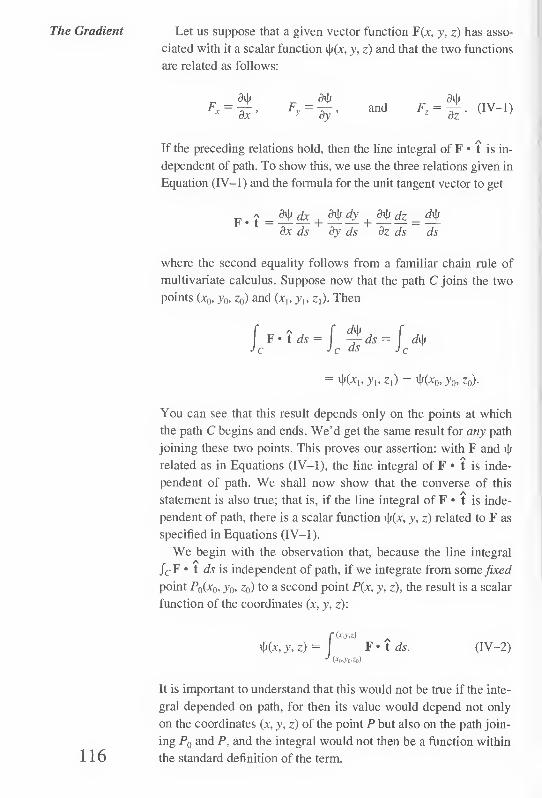
The Gradient Let us suppose that a given vector function F(x, y, z) has asso¬
ciated with it a scalar function i\j(x, y, z) and that the two functions
are related as follows:
Fr = 3»Jj
dx ' F
y dy ’ and (IV-1)
If the preceding relations hold, then the line integral of F • t is in¬
dependent of path. To show this, we use the three relations given in
Equation (IV-1) and the formula for the unit tangent vector to get
= = # dx ds dy ds dz ds ds
where the second equality follows from a familiar chain rule of
multivariate calculus. Suppose now that the path C joins the two
points (xQ, y0, z0) and (x,, yu z,). Then
= »K^i,3;i.zi) - »K*o. zo)-
You can see that this result depends only on the points at which
the path C begins and ends. We’d get the same result for any path
joining these two points. This proves our assertion: with F and v|i
related as in Equations (IV-1), the line integral of F • t is inde¬
pendent of path. We shall now show that the converse of this
statement is also true; that is, if the line integral of F • t is inde¬
pendent of path, there is a scalar function v|/(zc, y, z) related to F as
specified in Equations (IV-1).
We begin with the observation that, because the line integral
JCF • t ds is independent of path, if we integrate from some fixed
point P0(x0, Fo» Zo) to a second point P(x, y, z), the result is a scalar
function of the coordinates (x, y, z):
f(w)
i)j(x, y, z) = I F • t ds. (IV-2) ^ (■roJo.Za)
It is important to understand that this would not be true if the inte¬
gral depended on path, for then its value would depend not only
on the coordinates (x, y, z) of the point P but also on the path join¬
ing PQ and P, and the integral would not then be a function within
the standard definition of the term. 116

Line Integrals
and the Gradient
Since the integral we’re examining is path independent, we are
free to select any curve as the path of integration. We choose the
one shown in Figure IV-1. It consists of two parts. The first, C0,
Figure IV-1
connects P0 to an intermediate point P, whose coordinates are
(a, y, z), where a is some constant. Beyond fixing its two end points
and requiring it to be reasonably smooth, we do not need to specify
anything more about C0. The second part of the curve, Cj, is the
straight-line segment from Px to P. Thus, Equation (IV-2) becomes
v|)(x,y,z)=[ F'tds+f Fx(x', y, z) dx'. Jp0 Jp,
The first term on the right-hand side of this equation is indepen¬
dent of the variable x. The second term is, effectively, nothing
more than an ordinary one-dimensional integral, since y and z are
constant on C, and just come along for the ride. That is,
[ Fx(x', y, z) dx' = f Fx(x', y = const., z = const.) dx', J p, -'a
and so
3i|/
dx = const., z = const.) dx'
= FJx, y, z).
117 where we use the fact that the derivative of an integral with re¬
spect to its upper limit is merely the integrand evaluated at that
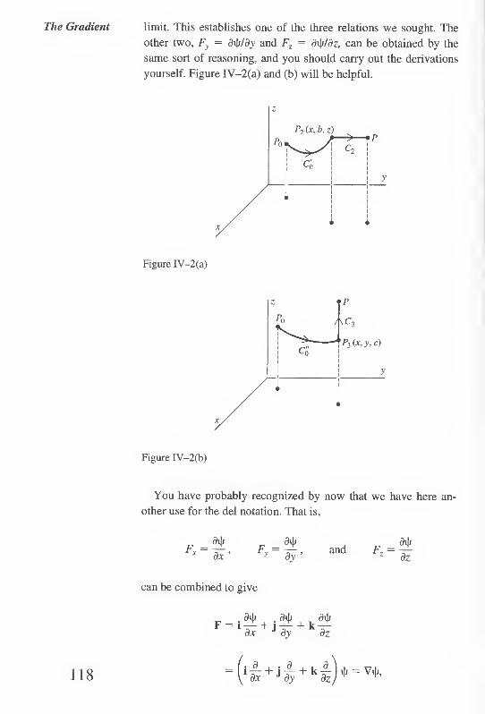
The Gradient limit. This establishes one of the three relations we sought. The
other two, Fy = di|i/dy and Fz = di|i/dz, can be obtained by the
same sort of reasoning, and you should carry out the derivations
yourself. Figure IV-2(a) and (b) will be helpful.
Figure IV-2(a)
Figure IV-2(b)

Line Integrals
and the Gradient
which is read “del psi.” This operator is called the gradient and is
sometimes written gradvj/. However, we shall always write Vili in,
keeping with modem usage. The gradient of i|i is a vector function of
position. Its geometric significance will be discussed in detail later.
We have now established the relationship between path inde¬
pendence and the existence of a scalar function r|r(jc, y, z) such that
F = Vv|r. Since there is also a relationship between path indepen¬
dence and the fact that V X F = 0, you may suspect that V X F = 0
and F = Vvjr are also related. Indeed, if F = Vvfi, then under suit¬
able conditions, V X F = 0. This is easily established. Consider,
for example, the x-component of V X F:
(V X F)v = dl±- dFy _ Q (dty
dy dz dy \dz
32v)/ d2i)f 0.
dy dz dz dy
dz\dy j
This last equality follows if vji and its first and second derivatives
are continuous, for then d2i|>/dy dz = 32i\i/dz dy. Obviously, the
other two components of V X F can be shown to vanish in ex¬
actly the same way. Thus,
3ilf Fq = 'dq Cq=x,y,Z) => V X F = 0.
The converse of what we have just shown would assert that if
V X F = 0, then there exists a scalar function vjr such that F = Vd),
a statement that is true, provided the region of interest is simply
connected. To understand this, we can consult Figure IV-3,
which shows how path independence of the line integral of F • t,
V X F = 0, and F = VvJ/ are related. The solid arrows in the dia¬
gram represent implications that hold in general, provided F is
smooth. The dashed arrows represent implications requiring not
only that F be smooth, but that the region of interest be simply
connected. We have already shown that (1) implies both (2) and
(3) and that (3) implies (1) in a simply connected region. Combin¬
ing these two statements, we see that (3) implies (2) in a simply
connected region.
In practice, just as the functions we deal with usually have con¬
tinuous first derivatives (and are therefore smooth), the regions
we work with are simply connected. In such circumstances we
can relax a bit and regard the three statements summarized in Fig- 119

The Gradient l. 2.
Figure IV-3
ure IV-3 as equivalent: each implies and is implied by each of the
others. However, you should be aware of simple connectedness
and its implications for the relations among the three statements.
To give a simple example of the ideas we have been dis¬
cussing, consider the vector function
F(x, y, z) = iy + jx.
This function is smooth everywhere, and we have already noted
that its curl is zero (page 92). According to what we have just
said, this means there must be a scalar function i|j(x, y, z) such that
F is its gradient. Thus, i|i must satisfy
= 0 =
dijj
dz '
Clearly, i|i(x, y, z) = xy + C, where C is an arbitrary constant, sat¬
isfies these relations. This should be contrasted with the case of
the function F = iy — jx, the curl of which does not vanish (page
92). If this function were the gradient of a scalar function i|j, we
should have
120

Finding the
Electrostatic
Field
but, as you should be able to convince yourself, there is no func¬
tion vji that satisfies these three equations.
The expression we have written for the gradient of a scalar
function i|j(x, y, z), namely,
. dil/ . di[< 54* V'J’ = 1^ + J^+k^'
is really just the form of this operator in Cartesian coordinates. To
find the form of the gradient in other coordinate systems, if you
go about it straightforwardly, is a tedious job. For example, to
find the gradient in cylindrical coordinates, we would first have to
express the Cartesian unit vectors i, j, and k in terms of the analo¬
gous quantities e,., e9, and e. in cylindrical coordinates. Then,
using x = r cos 0, y = r sin 0, and the chain rule for differentia¬
tion, we would have to express derivatives with respect to x, y,
and z in terms of those with respect to r, 0, and z. We shall not
pursue this matter here because later (see pages 141 ff.) an easier
and faster method will be available to us. For the present we
merely quote the form of the gradient in cylindrical and in spheri¬
cal coordinates.
Cylindrical:
rj i J#, J 1 dl|t » dtjl V^=e,.-^+ee7^+e;^.
Spherical:
„ , A 4 , A 1 # , A l # V 4* = e,.-r-+ e67—-+ e„—:—r —
or ^ ' dq> r sin cp 50
(IV-3)
(IV-4)
A coordinate-free definition of the gradient analogous to the ones
given for the divergence [Equation (11-17)] and the curl [Equa¬
tion (III—8)] is discussed in Problem IV-25.
Finding the Electrostatic Field
We began our discussion of vector calculus with a search for
some convenient method for finding the electrostatic field. Our in¬
vestigations led us to the differential form of Gauss’ law,
121 V • E = p/e0.

The Gradient Even this expression is not often useful for finding E because it is
one equation in three unknowns (Ex, Ey, and E, in Cartesian coor¬
dinates). Now, at last, we are able to complete our discussion and
write down the equations that are often the most useful of all
known methods for finding the field.
This final step rests on the observation that since
E • t ds = 0
for any closed path C, the field E can be written as the gradient of
a scalar function. Conventionally, this function, called the electro¬
static potential, is designated d>(x, y, z), and we write1
E = -vo>.
Combining this equation with the differential form of Gauss’ law
[Equation (11-17)], we get
V • (-Vd>) = p/e0,
or
V*(Vd>) = — p/e0.
When we write out the left-hand side of this equation in detail, we
find
V • (Vd>) Jl dx
a<t> . a<t>
dx J dy
d23> d2d> d2<£
dx2 dy2 dz2
and so
a2d> , d2<t> , a2d> , TT + TT + TJ = ~P/eo- dx dy dz
(IV-5)
Equation (IV-5) can be written more compactly by introducing
a new operator, called the Laplacian, which is denoted, for
122 1 The negative sign in this equation is not put there just to make life more difficult;
there is a good reason for it. See the discussion on page 139.

Finding the
Electrostatic
Field
fairly obvious reasons, by the symbol V2 (read “del squared”).
That is.
V2 = V • V d_
dx + j
_ V | U | u
dx2 dy2 dz2
In this new notation Equation (IV-5) becomes
V25> = — p/e0.
(IV-6)
(IV-7)
Equation (IV-fi) provides the form of the Laplacian in Carte¬
sian coordinates; its forms in cylindrical and spherical coordinates
will be given in the next section. The best definition of the Lapla¬
cian is probably
v2/= V.(V/),
where / is some suitably continuous scalar function of position.
This definition has the important advantage of being independent
of the coordinate system.
Equation (IV-7) is called Poisson’s equation. It is a linear,
second-order partial differential equation in one unknown, the
scalar function <fi(x, y, z), and is the culmination of our long
search for a method of determining the electrostatic field. A great
body of work exists describing the many elegant mathematical
schemes that have been devised to solve it, and a few simple ex¬
amples are given in the next section. In any problem, once we
have <£, the field is trivial to find using E = — Vfi).
At any point in space where there is no electric charge, the den¬
sity p is zero and Poisson’s equation reduces to
V23> = 0.
This is called Laplace’s equation and is more often used than
Poisson’s equation. The reason for this is that usually charges are
distributed over various objects; this gives rise to a field, and we
are interested in finding the potential (and from it, the field) in the
charge-free space between the objects. In the simplest of situa¬
tions it is possible to specify “boundary conditions,” that is, the
123 value of the potential on the surfaces of these objects (Figure

The Gradient
Figure IV-4
IV—4). We then find that solution of Laplace’s equation which
takes on the given values on the surfaces. This is illustrated in the
next section.
Using Laplace's Equation2
Whether solving Laplace’s equation is or is not a topic in vector
calculus is a moot point, but the basis of our entire discussion has
been a search for a method to calculate electric fields. Since
Laplace’s equation is the end product of that search, we can
scarcely omit a few examples to show how it works.
We begin with an especially simple problem. Imagine we have
two very large (“infinite”) parallel plates separated by a distance s
(Figure IV-5). Choosing a coordinate system as shown in the fig¬
ure, let the plate at x = 0 be held at zero potential and that at x = s
at V0. Our object is to find the potential and the electric field in the
space between the two plates. Because the plates are infinitely
large, there is nothing to distinguish a point (x, y, z) from any
other point (x, >■', z’) having the same x-coordinate. It follows that
the potential $ depends on x but not on y or z. Thus, V2<b reduces
in this case simply to d2(l>/dx2, and so Laplace’s equation and the
associated boundary conditions are
124 2 This section is not essential to what follows and may be omitted.
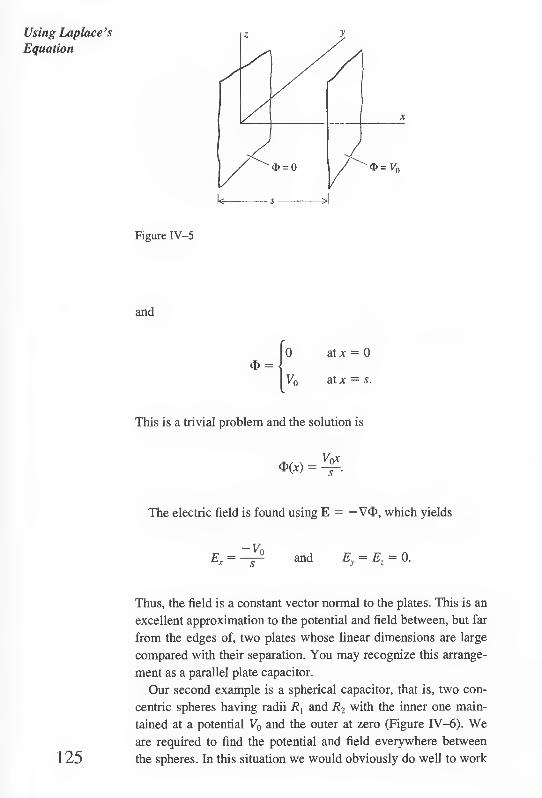
Using Laplace’s
Equation
Figure IV-5
and
<t> =
0 at x = 0
V0 at x = s.
This is a trivial problem and the solution is
^ Vox = —
The electric field is found using E = — V<I>, which yields
Ex = —^ and Ey = Ez = 0.
Thus, the field is a constant vector normal to the plates. This is an
excellent approximation to the potential and field between, but far
from the edges of, two plates whose linear dimensions are large
compared with their separation. You may recognize this arrange¬
ment as a parallel plate capacitor.
Our second example is a spherical capacitor, that is, two con¬
centric spheres having radii /?, and R2 with the inner one main¬
tained at a potential V0 and the outer at zero (Figure IV-6). We
are required to find the potential and field everywhere between
the spheres. In this situation we would obviously do well to work 125

The Gradient
Figure IV-6
in spherical coordinates r, 0, and 4>, in which Laplace’s equation
between the spheres has the imposing form
V2<f> = 1A r2dr
, i a / .
r2 sin (() 3<t> \ in d4>
(See Problem IV-23.) Fortunately, we need not work with this equa¬
tion as it stands; a little thought will convince you that can only be
a function of r, since there is no way to distinguish a point (r, 0, 4>)
from another (r, 0', 4>') with the same r but different 0 and 4>- Thus,
1 323>
r2 sin2 cf> 30‘ = 0.
3$ _ 3d> = n
30 3c() '
and Laplace’s equation reduces to
<iv-8)
We are interested in the solution of this equation that is valid for
f?, < r < R2 and satisfies the boundary conditions
D(r) = Vo at r — R,
126 o at r = R2.

Using Laplace’s
Equation Multiplying Equation (IV-8) by r2 and putting i|i = (IQ/dr, we get
d_
dr (r2i|/) = 0,
and so
r2v|i = c,,
where ct is a constant. Hence,
C\
r 2 ’
and it follows that
Q = ~ + c* (IV-9)
where c2 is another constant. Imposing the boundary conditions,
we find
R r + c2=Vo and
~i+c2=0’
whence
VoRlR 2
Rt- R
VqRi
Cl Ri-Ri'
Substituting these in the expression for the potential [Equation
(IV-9)], we get
To get the electric field, we must take the gradient of Q, and this
is clearly most conveniently done in spherical coordinates [see
Equation (IV-4)]. However, since in this case T* depends only on
r, we get only a radial component:
P _ _dQ _ Vq/?i/?2 1 r dr - R2 ’
127 £„ = £,!, = 0, (/?, < r < R2).

The Gradient
Figure IV-7
Our third and last example is more complicated (and more in¬
teresting) than the foregoing. If a potential difference is main¬
tained between two “infinite” parallel plates P and P' (Figure
IV-7), then we know from our first example that the field be¬
tween them is a constant vector normal to the plates. Choosing a
coordinate system as shown in the figure (with the z-axis out of
the plane of the paper), we have E = E0i, where E0 is a constant.
Let an “infinitely” long cylinder held at zero potential be situated
between the plates with its axis along the z-axis. Let its radius
R be small compared with the plate separation. What are the
potential and the electric field outside the cylinder and between
the plates? Here, clearly, we should use cylindrical coordinates
(r, 0, z), in which case Laplace’s equation reads
V2<D = IA r dr 2002 0Z2
(See Problem IV-21.) You should convince yourself that <I> in
this case must be independent of z, so this equation simplifies
somewhat to
li. r dr
d2<l>
■2 002 (IV-10)
There are two boundary conditions, of which the first is
d>(r, 0) = 0 at r = R.
128
The second condition has to do with the fact that at large values
of r, the influence of the cylinder is negligible and the field must

Using Laplace’s
Equation
be, to a good approximation, what it would be if the cylinder were
not present at all, that is, jE'0i. To put this in terms of the potential,
we note that
= -Enx
will provide just such a field. Since x = r cos 0, we can write the
second boundary condition
<l>(r, 0) = — E0r cos 0, r»R. (IV—11)
Let’s try to solve Laplace’s equation for this problem [Equa¬
tion (IV-10)] by assuming we can write
<t>(r, 0)=/(r)cos0, (IV-12)
where/(r) is an as yet unknown function. What prompts us to do
this is the fact that the second boundary condition [Equation
(IV—11)] has precisely this form—a function of r multiplied by
cos 0. If we substitute Equation (IV-12) into Equation (IV-10),
the result is a differential equation for the function/(r):
dj. \ V dr2 r dr
1 /= o.
Putting/(r) = rk where \ is a constant leads to
MX. - 1)^“2 + \rx~2 - rx~2 = 0,
or
k2= 1,
and X. = ±1. Hence we get
/(r)=Ar + |,
where A and B are constants. Thus, our solution is
129
$(r, 0) = ( Ar + j: j cos 0.

The Gradient The first boundary condition requires that
AR + | = 0,
or
B = —AR2.
Hence,
* AR2 0) = Ar cos 0-— cos 0.
To impose the second condition, we note that for r large, the second
term in this last equation is negligible compared with the first. Thus,
<I>(r, 0) — Ar cos 0, r large.
We satisfy the second boundary condition by choosing A = — E0.
The complete solution is thus
<J>(r, 0) = -E0r cos 0.
To find the electric field, we proceed as usual with E = —V<f>.
Using Equation (IV-3), we get
E0 1 + cos 0,
sin 0,
E. =
You should verify that for large r, this field reduces to E0i as
required.
You may find this last example disquieting, since a certain
amount of clever guesswork is used in finding the potential. Actu¬
ally, there are standard procedures that, in problems of this kind, lead
more or less straightforwardly to the solution. A discussion of these 130

Directional procedures, however, would be veiy lengthy and (in the well-worn
Derivatives and phrase) beyond the scope of this text. Before moving on, however,
the Gradient one further point is worth making: A solution of Laplace’s equation
that satisfies appropriate boundary conditions is unique. That is to
say, there is one and only one such solution, so that if we solve a
problem by guesswork and skullduggery, and someone else solves it
with refined and elegant mathematical techniques, the two solutions,
in spite of their disparate pedigrees, must be the same. In Problem
IV-24 you will be led through a proof of this remarkable fact.
Directional Derivatives and the Gradient
We have introduced the gradient as a sort of mathematical artifice
useful in discussing path-independent line integrals. We now turn
to a more detailed examination of the gradient in order to describe
its geometrical significance.
Before beginning our discussion, we make a few comments on
Taylor series, since these are needed in what follows. For a scalar
function of one variable that is suitably continuous and differen¬
tiable, we have
f(x + Ax) = f(x) + Axf'{x) + |(Ax)2/"(x) + ■ ■ •.
This says that the value of the function at some point x + Ax can be
written as the sum of (usually) infinitely many terms that involve the
function and its derivatives at some other point x. Among other
things, this Taylor series is useful for calculation, for if the two
points are close together (that is, if Ax is small), then we can truncate
the series after a certain number of terms (which we hope is small),
since the neglected terms, each proportional to some large power of
the small number Ax, will sum to a value that is negligible.
Taylor series can also be formed for functions of several vari¬
ables. Thus, for a function of two variables we have
fix + Ax, y + Ay)
= /(x,y) + AxJ£+ Ay^ + ---. (IV-13)
This says that the value of the function at some point (x + Ax,
y + Ay) can be written as a sum of (usually) infinitely many terms
131 that involve the function and its derivatives at some other point

The Gradient (.x, y). We shall never need the explicit form of the remaining
terms of this series [represented by the dots in Equation (IV—13)].
We should know, however, that these terms involve higher pow¬
ers of the “small” numbers Ax and Ay (for example, Ax2, Ay2,
AxAy, Ax3, Ay3, Ax2 Ay, and so on). With these simple ideas in
mind we turn now to our main task.
Consider some function z = f(x, y). Geometrically, this repre¬
sents a surface as shown in Figure IV-8(a). Let (x, y) be the coor¬
dinates of a point P in the xy-plane. The height of the surface
above this point is represented by the length of the dotted line PQ\
that is, PQ = z = fix, y). Suppose now we take a short step in the
xy-plane to a new point P' with coordinates (x -I- Ax, y + Ay).
The height of the surface above this point is P'Q' = /(x + Ax,
y + Ay). Let As be the length of the step (Ax = PP').
Figure IV-8(a)
We next ask how much the function/has changed as a result of
taking this step. Clearly, this change is the difference in the two
heights PQ and P'Q', and
P'Q' ~ PQ - A/ = /(x + Ax, y + Ay) -fix, y).
Applying the Taylor series formula stated above [Equation
(IV-13)], we get
A/ = /(x, y) + Ax ^ + Ay ^ + • • • - fix, y)
-zufGi, 132

Directional
Derivatives and
the Gradient
We now recast this expression by what at first may seem an un¬
necessary elaboration of the notation. Let As be a vector that has
magnitude As and points from P to P'. Clearly,
As = i Ax + j Ay.
But the gradient of/is
V/ = .df
1 dx
(an obvious specialization of the gradient notation to a function of
two, rather than three, variables). It follows at once that
A/ = (As) • (V/) + • • •.
Complicating matters slightly more, let u be a unit vector in the
direction of As. Then
As = u As
and
so that
A/= (u • V/) As + • ■ ■,
A/ — = u • V/ + As
We now take the limit of this equation to get
4f_ .. Af „ ~r = lim -r— = u • vf. ds 4s->o As
(IV—14)
There is no longer any need for “+ • • since the dots repre¬
sented terms that go to zero as As goes to zero.
This new expression [Equation (IV-14)] has a simple interpreta¬
tion: it is the rate of change of the function/(x, y) in the direction of
As (that is, of u). Redrawing Figure IV-8(a) and passing a plane
through P and P' parallel to the z-axis [Figure IV-8(b)], we see that
it cuts the surface z = fix, y) in a curve C. The quantity df/ds de¬
fined in Equation (IV-14) is the slope of this curve at the point O. 133

The Gradient z
Figure IV-8(b)
The quantity df/ds is called the directional derivative of /. Al¬
though the analysis given earlier that led to this derivative was for
functions of two variables, the results all apply to functions of
three (or more) variables. Thus,
Jr F(x, y, z) = u • VF
is the rate of change of the function F(x, y, z) in the direction
specified by the unit vector u. An example of the directional derivative may be amusing here.
We’ll work with a function of two variables so that we can draw
pictures. Thus, let’s consider
z =f(x,y) = (x2 + y2),/2.
which is an inverted right circular cone whose axis coincides with
the z-axis [see Figure IV-9(a)]. We ask for the directional deriva¬
tive of this function at some point x = a and y = h and in the di¬
rection specified by u = i cos 0 + j sin 0 [see Figure IV-9(b)].
First we need the gradient of f(x, y). But
dl dx
x z and
= y dy Z’
as you can easily verify. Thus,
V/ = ix + jy
134 z

Directional
Derivatives and
the Gradient
Figure IV-9(a)
Figure IV-9(b)
and
df A _ x cos 0 + y sin 0 a cos 0 + b sin 0 — = u • Vr —->- --. ds 2 Va2 + b2
Suppose 0 is chosen so that u is in the radial direction as indi¬
cated in Figure IV-9(c). This means
cos 0 = a
{a2 + b2)112'
sin 0 h
{a2 + b2)112'
and so
df_ _ a _ a_b . b
ds Va2 + b2 Va2 + b2 Va2 + b2 Va2 + b2
135 The significance of this result is brought out in Figure IV-9(d).

The Gradient
Figure IV-9(c)
Figure IV-9(d)
A second interesting case is that in which u is chosen perpen¬
dicular to the direction of the previous example [see Figure
IV-9(e)]. We then have
cos 0 = —b
(a2 + bY2’
sin 0 a
0a2 + b2)m’
and so
df_ a ( b \
ds Va2 + b2 V Va2 + b2)
+ -- b f—g- Va2 + b2 Wa2 + b1
136 The meaning of this result is illustrated in Figure IV-9(f).

Geometric
Significance of
the Gradient
Figure IV-9(e)
Figure IV-9(f)
Geometric Significance of the Gradient
With the concept of the directional derivative at our disposal, we
are now in a position to give a geometric interpretation of the gra¬
dient. At some point P0 with coordinates (x0, y0, z0) we have
where the subscript 0 means the quantity is to be evaluated at the
point (x0, y0, z0). Now (VF)0, the gradient of F evaluated at P0,
may be represented by an arrow emanating from that point as
shown in Figure IV-lO(a). If we ask in what direction we must
move to make (dF/ds)0 as large as possible, it is clear that u
should be in the same direction as (VF)0. This is because if we let
a be the angle between u and (VF)0, then (dF/ds)0 = |VF|0 cos a,
and this is as large as it can be when a = 0. Thus, the gradient of 137

The Gradient
Figure IV-lO(a)
a scalar function F(x, y, z) is a vector that is in the direction in
which F undergoes the greatest rate of increase and that has
magnitude equal to the rate of increase in that direction.
To illustrate this interpretation of the gradient, let us go back to
the inverted cone z = f(x, y) = (x2 + y2)m we discussed earlier.
We learned that
V/ = >-* + j y
z
and
£ ds
a cos 0 + sin 0 0(6).
To find the direction in which /(x, y) undergoes the greatest rate
of change, we set
dD _ —a sin 8 + b cos 8
M VcfHf
This gives tan 0 = b/a, whence cos 0 = al{a2 + b2)1'2 and sin 0 =
b/(a2 + b2)m. So (df!ds)mm = 1. On the other hand.
|V/| = ^+y2
= 1,
since z2 = x2 + y2. Furthermore, tan 0 = b/a corresponds to the
direction a\ + bj, while at the point (a, b),
V/ = ai + bj
(a2 + b2)m’
138

Geometric which is a vector in the same direction. Thus both properties of
Significance of the gradient are illustrated; it’s in the direction of maximum rate
the Gradient of increase, and its magnitude is equal to the rate of increase in
that direction.
As a second example of the interpretation of the gradient, we con¬
sider the plane z = f(x, y) = \ — x — y shown in Figure IV-10(b).
It’s easy to see that V/= —i — j. Using u = i cos 0 + j sin 0 as be¬
fore, we find df/ds = u • V/ = -cos 0 - sin 0 = Z)(0). Thus
dD
d% sin 0 — cos 0 = 0,
Figure IV-10(b)
which yields 0 = tt/4 or 5tt/4. The second derivative test shows
that tt/4 corresponds to a minimum and 5tt/4, to a maximum. It
can be seen from Figure IV-10(b) that the greatest rate of in¬
crease is indeed at an angle of 5n/4. Moreover, the greatest rate of
increase is
139
= D(5ir/4) = V2,
whereas |V/| = |—i — j| = V2. Again, both properties of the gra¬
dient are illustrated by this example.
With this geometric interpretation of the gradient at our disposal,
we can now see the reason for the negative sign in the equation
E = — V<F: Since V<F is a vector in the direction of increasing <f>, the
force on a positive charge q is F = qE = —<?V<F, which is in the di¬
rection of decreasing <J>. Thus, the negative sign ensures that a pos¬
itive charge moves “downhill” from a higher to a lower potential.
There is another property of the gradient useful in understand¬
ing its geometric significance. To make this discussion concrete,
let T(x, y, z) be a scalar function that gives the temperature at

The Gradient
Figure IV-11
any point (x, y, z). The locus of all points having the same temper¬
ature T0 is (in the simplest case) a surface whose equation is
T(x, y, z) = T0 (Figure IV-11). This is called an isothermal sur¬
face. We now show that VT is a vector normal to the isothermal
surface. Let C be any curve lying in the isothermal surface and let
P be any point on C. Let u be the unit vector tangent to C at P (it
doesn’t matter which direction along C we take). The directional
derivative in the direction u is
because T does not change as we move along the isothermal sur¬
face. If the scalar product of two vectors, neither of them zero,
vanishes, the two vectors are perpendicular. Thus VT is perpen¬
dicular to C at P. By the same argument it is perpendicular to any
curve on the surface through P (such as C' in Figure IV-11). But
this can be true only if VT is normal to the isothermal surface at
P. In general then, V/(;c, y, z), where f(x, y, z) is a scalar function,
is normal to the surface f(x, y, z) = constant?
A simple example of this property of the gradient is provided
by the function F(x, y, z) = x2 + y1 + z2. The surface F{x,y,z) =
constant is, of course, a sphere (assuming the constant is posi¬
tive). As you should verify for yourself, VF = 2(ix + jy + kz) =
2r. Thus, we have a familiar result: A vector normal to a spherical
surface is in the radial direction. We’ll leave it to you to ponder
the geometric relation between the electrostatic field E and its
equipotential surfaces <I>(x, y, z) = constant.
3 The connection between this property of the gradient and our earlier expression
for the unit vector normal to a surface [Equation (II-4)] is the subject of Problem
140 rv-2o.

The Gradient in Cylindrical and Spherical Coordinates
We can make a simple connection between the property of the
gradient just discussed and the fact that it is in the direction of
the greatest rate of increase. Any displacement from the surface
f{x, y, z) = constant, regarded as a vector s, can be resolved into a
component along the surface (s||) and one normal to it (sj, as
shown in Figure IV-12. That part of the displacement along the
surface is “wasted motion” if our aim in moving is to cause a
change in the value of f{x, y, z). Only the normal component car¬
ries us away from the surface and causes a change in/. From this
it is clear that the greatest increase possible for a given magnitude
of displacement should occur when we move away from the sur¬
face in the normal direction. But we have already established that
the greatest rate of increase occurs in the direction of the gradient.
Thus the gradient is normal to the surface.
A
Figure IV-12
The Gradient in Cylindrical and Spherical Coordinates
A by-product of our discussion of the directional derivative is the
“easier and faster” method for calculating the gradient in spherical
and cylindrical coordinates mentioned earlier (see page 120). To de¬
termine this method, we begin by outlining our derivation of dflds:4
1. Our first step is to consider a scalar function of three Carte¬
sian coordinates/(x, y, z) and use Taylor series to determine
the change in / caused by a displacement from the point
(x, y, z) to a second point (x + Ax, y + Ay, z + Az). We find
for this change
A/= y Ax + y Ay + y Az + • • • - J dx dy dz
4 The calculation outlined here pertains to a function of three variables and is a
simple generalization of the calculation on pages 130-133, which deals with a
141 function of two variables.

The Gradient 2. We next write A/in terms of As, the vector displacement from
(x, y, z) to (x + Ax, y + by, z + A z). Clearly (see Figure
IV—13),
so that
As = i Ax + j Ay + k Az.
Af = • As H-.
Figure IV-13
3. Finally, we write As = u As, divide by As, and take the limit:
Af_df . df df df\ A limT- = T=1r + J3“ + ,!F'u-
a.v—>o As ds \dx ay dz /
The quantity that is dotted into u in this last expression is
then recognized as the gradient of/in Cartesian coordinates.
To obtain the gradient of a scalar function in cylindrical coordi¬
nates we proceed in much the same way:
1. We consider a scalar function of three cylindrical coordi¬
nates,/(r, 0, z). Using Taylor series, we find the change in/
due to a displacement from the point (r, 0, z) to a second
point (r + Ar, 0 + A0, z + Az):
Af=yAr + ^Ad + ^Az + dr 50 dz
2. Next, we write A/in terms of As. This is the heart of the cal¬
culation. From Figure IV-14 we have
142 As = e,. Ar + e„r A0 + e, Az.

z The Gradient
in Cylindrical
and Spherical
Coordinates
Figure IV-14
Two features of this expression require some discussion. First,
the displacement in the direction of increasing 0 (of magnitude
r A0) is an arc of a circle rather than a straight line segment.
However, since we will eventually pass to the limit as A.v —» 0,
we may regard A0 (as well as Ar and A") as arbitrarily small,
in which case the arc is arbitrarily close to its subtending
chord. Thus, as indicated in Figure IV-15, Ar, r A0, and Az
Figure IV-15
approximate to any desired degree of accuracy three mutually
perpendicular displacements, the analogs of the three Carte¬
sian displacements Ax, Ay, and Az (see Figure IV-13).
The second feature of our expression for As that requires
comment also has to do with the displacement in the direction
of increasing 0. It is this: Since the arc is part of a circle of ra¬
dius r + Ar, we should, strictly speaking, write the displace¬
ment as (r + Ar) A0, not r A0. But the additional term Ar A0
is “second order”; that is, it is the product of two small quan¬
tities and therefore negligible compared with r A0.
If we now write our expression for A/in terms of As, we get

The Gradient Note the factor 1/r in the second term to compensate for the
factor r in eer A0 in As.
3. Finally, putting As = u As, we find
r Af_df lim T- = -T-
As—»o As ds
A
• u.
The quantity in the preceding expression dotted into u is the
gradient of/in cylindrical coordinates.
An analogous procedure can be used to find the gradient in
spherical coordinates; this has been left as an exercise (see Prob¬
lem IV-22).
PROBLEMS
IV-1 (a) Calculate F = V/for each of the following scalar functions:
(i) /= xyz.
(ii) /= x2 + y2 + z2.
(iii) f=xy + yz + xz.
(iv) /= 3a2 - 4Z2.
(v) /= e~x sin y.
(b) Verify that
F • t ds = 0
for one or more of the functions F determined in part (a) choosing
for the curve C:
(i) the square in the Ay-plane with vertices at (0, 0), (1, 0),
(1, 1), and (0, 1).
(ii) the triangle in the yz-plane with vertices at (0, 0), (1, 0),
and (0, 1).
(iii) the circle of unit radius centered at the origin and lying
in the xz-plane.
(c) Verify by direct calculation that V X F = 0 for one or more
of the functions F determined in part (a).
lV-2 Verify the following identities in which/and g are arbitrary differ¬
entiable scalar functions of position, and F and G are arbitrary differ¬
entiable vector functions of position.
(a) V(/g) =/Vg + gVf
(b) V(F • G) = (G • V)F + (F • V)G + F X (V X G) + G X
(V X F).
(c) V • (/F) = / V • F + F • V/.
(d) V • (F X G) = G • (V X F) - F • (V X G).
(e) V x (fF) =/V x F + (V/) x F.
(f) V X (F X G) = (G • V)F - (F • V)G + F(V • G) -G(V • F).
(g) V X (V X F) = V(V • F) - V2F.
144

Problems IV-3 Show that V X V/ = 0 where f(x, y, z) is an arbitrary differentiable
scalar function. Assume that mixed second-order partial derivatives
are independent of the order of differentiation. For example, d2f/dx dz,
= d2f/dz dx.
TV-4 (a) Each of the following functions is smooth in a simply con¬
nected region. Determine which of them may be written as the
gradient of a scalar function, and for those that can, use Equation
(IV-2) to find that scalar function.
(i) F = iy.
(ii) F = Ck, C a constant.
(iii) F = iyz + jxz + kxy.
(iv) F = ix + jy -1- kz.
(v) F = ie~z sin y + je ' sin z + ke~r sin y.
(b) Neither of the following functions is smooth everywhere.
Nonetheless each can be written as the gradient of a scalar func¬
tion. Use Equation (IV-2) to find that scalar function.
(i) F = r/r2, r = u + jy.
(ii) F = r/r112, r = ix + jy + kz.
IV-5 The function F(r, 0, z) defined in Problem III—17 is smooth and has
zero curl in a nonsimply connected region consisting of all of three-
dimensional space with the z-axis removed. Show that there is no
scalar function vjr such that F = Vi|j by evaluating the line integral of
F • t from the point P,(0, —1, 0) to the point P2(0, 1, 0) over two dif¬
ferent paths: CR, the right-hand side of the circle of radius 1 lying in
the xy-plane and centered at the origin (see figure), and CL, the left-
hand side of the same circle. Orient the paths as shown. Why does the
fact that the two paths give different results imply that there is no
scalar function i|< such that F = Viji?
1V-6 (a) An electric dipole of strength p situated at the origin and ori¬
ented in the positive z-direction gives rise to an electrostatic field
—^ (2er cos 4> + e* sin <)>) 4ire0 r
145 E(r, 0, 4») =

The Gradient
Use Equation (IV-2) to show that the dipole potential is given by
1 p cos d> <h(r, 0, 4>) = ---—
4tt€0 r2
Useful information: In spherical coordinates,
* /v dr . * d§ ^ . , d6
t = e^+e*r^+e“''Sln<l>^
(b) Calculate the flux of the dipole field through a sphere of ra¬
dius R centered at the origin.
(c) What is the flux of the dipole field over any closed surface
that does not pass through the origin?
lV-7 Here is a “proof” that there is no such thing as magnetism. One of
Maxwell’s equations tells us that
V • B = 0,
where B is any magnetic field. Then using the divergence theorem, we
find
JJ B’fidS = J j J v • B dV = 0.
Because B has zero divergence, we know (see Problem III—24) there
exists a vector function, call it A, such that
B = V X A.
Combining these last two equations, we get
JJ n • VX At/S = 0.
Next we apply Stokes’ theorem and the preceding result to find
A’t ds = J J n • V X A dS = 0.
146 Thus we have shown that the circulation of A is path independent. It
follows that we can write A = Vi|), where i|) is some scalar function.

Problems Since the curl of the gradient of a function is zero, we arrive at the re¬
markable fact that
B = V X V4» = 0;
that is, all magnetic fields are zero! Where did we go wrong? [Taken
from G. Arfken, Amer. J. Phys., 27, 526 (1959).]
IV-8 Fick’s law states that in certain diffusion processes the current den¬
sity J is proportional to the negative of the gradient of the density p;
that is, J = —kVp, where A: is a positive constant. If a substance of
density p(jc, y, z, t) and velocity v(x, y, z, t) diffuses according to Fick’s
law, show that the flow is irrotational (that is, V X v = 0).
TV-9 (a) A substance diffuses according to Fick’s law (see Problem
IV-8). Assuming the diffusing matter is conserved, derive the
diffusion equation
(b) Bacteria of density p diffuse in a medium according to Fick’s
law and reproduce at a rate Xp per unit volume (X is a positive
constant). Show that
^ = k V2p + Xp.
1V-10 (a) A fluid is said to be incompressible if its density p is a con¬
stant (that is, is independent of x, y, z, and t). Use the continuity
equation to show that the velocity v of an incompressible fluid
satisfies the equation V • v = 0.
(b) If V X v = 0, the fluid flow is said to be irrotational. Show
that for an incompressible fluid undergoing irrotational flow,
v24> = o,
where <J>, a scalar function called the velocity potential, is so de¬
fined that v = V<t>-
IV-11 The heat Q in a body of volume V is given by
e-'lffw where c is a constant called the specific heat of the body, and T(x, y, z, t)
and p(x, y, z) are, respectively, the temperature and density of the
body. (Note that we are assuming the density to be independent of
time.) The rate at which heat flows through S, the bounding surface of
the body, is given by
dQ
dt n • VTdS, 147

The Gradient where k (assumed constant) is the thermal conductivity of the body,
and the integral is taken over the surface S bounding the body. Use
these facts to derive the heat flow equation
where a = cp/k.
IV-12 In nonrelativistic quantum mechanics a particle of mass m mov¬
ing in a potential V(x, y, z) is described by the Schrodinger equation
—V2»|; + WJr = ih^~, 2m T v dt
where h is Planck’s constant divided by 2tt and \\i(x, y, z, t), which is
complex, is called the wave function. The quantity p = is inter¬
preted as the probability density.
(a) Use the Schrodinger equation to derive an equation of the form
and obtain thereby an expression for J in terms of 4<> 4**’ m-
and h.
(b) Give an interpretation of J and of the equation derived in (a).
IV-13 (a) Find the charge density p(x, y, z) that produces the electric
field
E = g(ix + jy + kz),
where g is a constant.
(b) Find an electrostatic potential <J> such that — Vd> is the field E
given in (a).
(c) Verify that V2d> = — p/e0.
IV-14 (a) Starting with the divergence theorem, derive the equation
(u Vv) dS = V2v + (Vu) • (Vu)] dV,
where u and v are scalar functions of position and S is a closed
surface enclosing the volume V. This is sometimes called the first
form of Green’s theorem.
(b) If V2u = 0 use the first form of Green’s theorem to show that
J J n • (u Vu) dS = J J | Vu p dV,
where |V«p = (Vu) • (Vu).
(c) Use the first form of Green’s theorem to show that
JJL* (u Vv — v Vu) dS = III ^~ V 148 This is the second form of Green’s theorem.

Problems IV-15 An equation of the form
where / is a twice-differentiable function of position and time, is
called a wave equation. It describes a wave propagating in space
with velocity v. Use Maxwell’s equations (Problem III—20) to show
that in the absence of charges and currents (that is, p and J both
zero), all three Cartesian components of both E and B satisfy a wave
equation with v = c, where c = 1/Ve0p,0 is the velocity of light. For
example.
V2£, 1 d% c2 di2 '
Thus, the existence of electromagnetic waves traveling in empty space
with the velocity of light is a consequence of Maxwell’s equations.
TV-16 (a) In the text we found the potential and field for the case of an
infinite cylinder between parallel plates with the cylinder held at
zero potential. How must the solution be modified if the cylinder
is held at a potential V0 + 0?
(b) Show that there is no net charge on the cylinder.
1V-17 (a) A sphere of radius R is situated between two very large paral¬
lel plates that are separated by a distance s. A potential difference
is maintained between the plates and the sphere is held at zero po¬
tential. Find the potential and field everywhere outside the sphere
and between the plates. Assume that R « s.
(b) Show that there is no net charge on the sphere.
(c) Repeat part (a) assuming the sphere is held at a potential
v0*o.
IV-18 Let f(x, y) be a differentiable scalar function of x and y, and let
u = i cos 0 + j sin 0. Transform to a rotated coordinate system x', y'
such that x' is parallel to u (see the figure). Show that the directional
derivative in the direction of u is given by.
ds fi -V/ =
df_
dx''
149 0 x

The Gradient TV-19 You are at a point (a, b, c) on the surface
Z = (r2 ~ x2 - y2)m (z > 0).
Assuming both a and b are positive, in what direction must you move
(a) so that the rate of change of z will be zero?
(b) so that the rate of increase of z will be greatest?
(c) so that the rate of decrease of z will be greatest?
Draw a sketch to show the geometric significance of your answers.
TV-20 The unit vector normal to the surface z = f(x, y) is given by
[see Equation (II—4)]. We have also established that VF is a vector
normal to the surface F(x, y, z) = const, (page 140) so that VF/|VF| is
a unit vector normal to the surface F(x, y, z) = const. Show that these
two expressions for the unit normal vector are identical if F(x,y,z) =
const, and z = f(x, y) describe the same surface.
TV-21 Use the results of Problem 11-18 and the expression for the gradi¬
ent in cylindrical coordinates (see page 144) to obtain the form of the
Laplacian in cylindrical coordinates given on page 129.
IV-22 Using the procedure outlined in the text (pages 141-144) obtain
the expression for the gradient of t|i in spherical coordinates:
di|r 1 # r-r , 1 t . /v V4< = e,.—+ e*77X+ e 4> r dc|)
i #
1 r sin 4> 50
IV-23 Use the results of Problem 11-19 and the expression for the gradi¬
ent in spherical coordinates derived in Problem IV-22 to obtain the
form of the Laplacian in spherical coordinates given on page 126.
IV-24 Suppose you find a solution of Laplace’s equation that satisfies
certain boundary conditions. Is this solution unique or are there oth¬
ers? This problem will answer that question in certain simple cases.
Consider the region of space completely enclosed by a surface S0 and
containing in its interior objects 1, 2, 3,. .. (two of which are pictured
in the diagram). Suppose that S0 is maintained at a constant potential
<I>0, object no. 1 at <t>h object no. 2 at <J>2, and so on. Then in the
charge-free region R enclosed by S0 and between the objects, the po¬
tential must satisfy Laplace’s equation
V2<E> = 0
and the boundary conditions
<J> =
$0 on so 4), on S,
dL on S2
150

Problems
The following steps will guide you through a proof that <t> is unique.
(a) Assume that there are two potentials u and v, both of which
satisfy Laplace’s equation and the boundary conditions listed ear¬
lier. Form their difference w = u — v. Show that V2w = 0 in R.
(b) What are the boundary conditions satisfied by w?
(c) Apply the divergence theorem to
(l n • (w Vw) dS,
where the integration is carried out over the surface S0 + 5, + S2
H-, and show thereby that
/// lVw,l2dV=0,
where V is the volume of the region R.
(d) From the result of (c) argue that Vw = 0 and that this, in turn,
means w is a constant.
(e) If w is a constant, what is its value? (Use the boundary condi¬
tions on w to answer this.) What does this say about u and u?
(f) The uniqueness proof outlined in (a) to (e) involves specify¬
ing the value of the potential on various surfaces. Might we have
specified a different kind of boundary condition and still proved
uniqueness? If so, in what way or ways would the proof and the
result differ from those given above?
IV-25 In the text we defined the gradient in terms of certain partial de¬
rivatives. It is possible to give an alternative definition similar in form
to our definitions of the divergence and the curl. Thus,
1 //,"fis- V/= lim
av-.o AV j js
Here/is a scalar function of position, S a closed surface, and AV the
volume it encloses. As usual, n is a unit vector normal to S and point¬
ing out from the enclosed volume.
(a) Following a procedure similar to the one used in the text in
treating the divergence, integrate over a “cuboid” and show that
the preceding definition yields the expression
df df 3/ v/= i/ + jr- + k^-. dx dy dz 151

The Gradient (b) Use the alternative definition of the gradient given above to
show that the directional derivative of/in the direction specified
by the unit vector u is given by
ds = u • V/.
[Hint: Evaluate
S-fl nfds = J J u • nfdS
over a small cylinder (length As, cross-sectional area A4; see fig¬
ure) whose axis is in the direction of the constant unit vector u.
Then divide by the volume of the cylinder (As AA) and take the
limit as the volume approaches zero.]
(c) Arguing as we did in the text in establishing the divergence
theorem, use the alternative definition of the gradient to show that
If,**-Iff w where S is a closed surface enclosing the volume V.
(d) Obtain the relation stated in (c) directly from the divergence
theorem. [Hint: In ffsF• n dS = fffvV'FdVputF = ef where
e is a constant unit vector.]
152 x
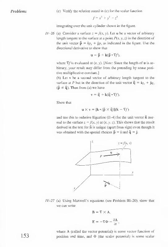
Problems (e) Verify the relation stated in (c) for the scalar function
/=*2 + y2 + z2
integrating over the unit cylinder shown in the figure.
IV-26 (a) Consider a surface z = fix, y). Let u be a vector of arbitrary
length tangent to the surface at a point P(x, y, z) in the direction of
the unit vector p = ipx + jpy as indicated in the figure. Use the
directional derivative to show that
u = p + k(p • V/),
where V/ is evaluated at (x, y). [Note: Since the length of u is ar¬
bitrary, your result may differ from the preceding by some posi¬
tive multiplicative constant.]
(b) Let v be a second vector of arbitrary length tangent to the
surface at P but in the direction of the unit vector q = iqx + ky
(p + q). Then from (a) we have
v = q + k(q • V/).
Show that
u X v = [k • (p X q)](k - V/)
and use this to rederive Equation (II—4) for the unit vector n nor¬
mal to the surface z — fix, y) at (x, y, z). This shows that the result
derived in the text for n is unique (apart from sign) even though it
was obtained with the special choices p = i and q = j.
TV-27 (a) Using Maxwell’s equations (see Problem III—20), show that
we can write
B = V X A,
E = -V<t> ot
153 where A (called the vector potential) is some vector function of
position and time, and (the scalar potential) is some scalar

The Gradient function of position and time, provided A and d> satisfy the
equations
+ -.)t (V • A) = — p/e0,
n 2 a
V2A - p.0eQ ~ = -|XoJ + V V • A + p,0e0 dt
(b) Show that if we define two new potentials
A' = A + Vx,
cp' = <p - ^ at’
where x is an arbitrary scalar function of position and time, then
B = V X A',
E = -V4>' - dt
That is, the fields E and B are not modified by the change in the
potentials A and d>. The change from (A, d>) to (A', fl>') is called
a gauge transformation.
(c) Show that if we require \ to satisfy the equation
V’ d2X V X - eoM-o = V • A + e0p,0
dt
then
V ' A +e0p,0—= 0.
(d) If x satisfies the equation given in (c), show that A' and <t>'
satisfy the equations
V2<D' a2<!>' _
eo(Xo ^ - e0
and
V2A' a2A' _ _ T 60P-0 n ~ M-oJ-
oV
The point to all of this is that we can make a gauge transformation [as
in (b)], impose the condition given in (c), and thereby obtain a scalar
and a vector potential that satisfy the equations in part (d), which are
wave equations with source terms proportional to p and J.
IV-28 The equation of motion of an ideal fluid can be written
§ + (v-V)v dV
154 where V is the volume of the fluid and 5 is its surface. Here fext(x, y, z)
is the external force per unit mass acting on the fluid, p(x, y, z) is the

Problems pressure of the fluid, and p(x, y, z) is its density, all at a point (x, y, z) in
the fluid, and v(x, y, z, t) is the velocity of the fluid at the point (x, y, z)
and at time t.
(a) Use the form of the divergence theorem given in Problem
IV-25(c) to rewrite the equation of motion of an ideal fluid in the
form
fext “ £ VP = + (v * V>v-
(b) Show that in the static case (v = 0), the equation of motion
becomes
fext = (1/p) Vp.
(c) Consider a column of incompressible fluid oriented vertically
parallel to the z-axis as shown in the figure. Assuming that the
only external force acting on the fluid is the downward uniform
gravitational attraction of the earth, apply the equation for the
static case given in (b) to show that
P=Pn~ P8Z
where g is the acceleration due to gravity and p0 is a constant.
155

Solutions to Problems
One must learn by doing the thing; for
though you think you know it, you have no
certainty until you try.
Sophocles
Chapter I
3. (a) (k + jyyVx2 + y2.
(b) (i + JXx + y)W2.
(c) -iy+jx.
(d) (k + jy + kz)/Vx2 + y2 + z2. 4. (a) (a2 cos2 wt + b2 sin2 ml)'11.
(b) —icoa sin mt + jo>b cos wt (velocity).
—ico2a cos wt — jofb sin to? (acceleration).
i 1
2tT60 (y2 + 1)3/2 '
156

Solutions to
Problems
Chapter II
6. In the following, c is an arbitrary constant.
y2 = c. (a) x2
(b) y = x + c.
(c) xy = c.
(d) v = c.
/ =
(e) x = c.
(f) x2
(g) y = W +
(h) y = ce?.
c.
c.
1. (a) (i+j + k)/V3.
(b) -(ix + jy - kz)/V2z.
(c) ix + kz.
(d) (—2ix — 2jy + k)Vl + 4z.
(e) (ix + jy + ka2z)/aV 1 + (a2 — l)z2.
3. [-i(dg/dx) - k(dg/dz) + j]/Vl + (dg/dx)2 + (dg/dz)2
fory = g(x, z).
[-j (dh/dy)
4. (a) V3/6.
k(dh/dz) + i]/V 1 + (dh/dy)2 + (dh/dz)2
for x = h(y, z).
(b) |(V5- 1).
(c) ir/2.
5. (a) 0.
(b) 2ira3.
(c) 3Tt/2.
6. 4h/?2(t0/3.
7.
8. 0.
9. ttr2X./ie0.
10. (a) 0. (c) 4’nR7'e~R\
(b) 4-rrR2h In /?. (d) [E(b) - E(0)]b2.
11. (a) E = cri/2e0, x > 0, and ~CTi/2e0, x < 0.
(b) E = p0fei/en, x> b\ poxi/e0, —b SiSi;
and — p0hi/e0, x < —b.
(c) E = ± (p0h/e0)(l — e 1''|/4)i (+ forx > 0, — forx < 0)
12. (a) E = (X/ltieQ)er/r
(b) E = (poh2/2e0)er/r, r>i>, and (p0r/2e0)er,r<b.
(c) E = (pnh2e0)(l/r)[l - (1 + rlb)e~rlh]%r.
13. (a) E = (Z?3p0/3€0)er/r2, r> b,
(po/3e0)i-er, r < b.
(b) E = i3p0/e0)(l/r2)[2 - (r2/*2 + 2rib + 2)e"r,6]er.
(P</3€0)r®i-. f < fc, (c) E = (l/3e0)(l/r2)[fc3p0 + (r3 - fe3)Pi]er, b<r<2b,
(f>3/3e0)(l/r2)(p0 + 7p,)er r > 2b.
The field is zero for r > 2b if p, = — p0/7. The total charge is then zero.
157

Solutions to
Problems 14. (a) 2(x + y + z).
(b) 0.
(c) ~(e~x + e~y + e-*).
(d) 2z.
(e) -y/tf+y2).
(f) 0. (g) 3.
(h) 0.
15. Surface integral equals 2s’’(x0 + y0 + z0) for the function of Problem
II-14a.
Surface integral equals 0 for function of Problem II-14b.
Surface integral equals s2(e~s/2 — es'2)(e~x" + e~y° + e~z,:) for func¬
tion of (II—14c).
16. (b) V • G = 0.
22. /(r) = constant/r2.
23. (a) 3b\
(b) 3ixR2h/4.
(c) 4'tr/?4.
24. (b) irR2B.
Chapter III
3. (a) 2(—iy + jz + kx).
(b) 5jx.
(c) ie~z + je~x + ke-v.
(d) 0.
(e) —ix — jy +
(f) 2(iy — jx).
(g) iz - kx.
(h) 0.
2kz.
(b)
(c) n
158
4. Line integral equals 2x0.v2 for function of Problem III-3a.
Line integral equals 0 for function of Problem III—3b.
Line integral equals s(e!l2 — e~sl2)e~y° for function of Problem III-3c.
Line integral equals 0 for function of Problem III—3d.
5. (a) a112 + a213
2 /l , cA 1 „ V5 \2 + 3/ ^ as a ^ °
■ V x F = (1 + 2>>) = aty = 0 V3 V3
13. (d) and (h).
15. (a) Line integral and surface integral equal 1.
(b) Line integral and surface integral equal — 3ir/4.
(c) Line integral and surface integral equal — 2-nR2.
19. 3/e.
25. If V • G = 0, then G = V X H
(a) H = Ijx2 +k [\y2 - (x - x0)z].
(b) H = jBqX.
(c) V • G * 0.
(d) H = -j(x - x0)z 4- k(x -I- x0)y.
(e) V • G + 0.
[Note: Your results may differ from these by additive constants/

Solutions to
Problems
a A
28. (a) 4>CH • t ds = ffsG • n dS where 5 is a capping surface of the
closed curve C.
29. (d) Surface and volume integral each equal i - j — k.
Chapter IV
1. (a) (i) F = tyz + jxz + kxy.
(ii) F = 2(k + j>’ + kz).
(iii) F = i(jy + z) + jU + z) + k(x + y).
(iv) F = 6ix — 8kz.
(v) F = — ie~x sin y + je~* cos y.
4. (a) (i) Not path independent.
(ii) i|; = cz + const.
(iii) i|/ = xyz + const.
(iv) v|» = {(x2 + y2 + z2) + const.
(v) Not path independent.
(b) (i) i|» = In r + const.
(ii) vjr = \rm + const.
13. (a) p = 3ge0.
(b) <I> = ~{gC + y2 + z2).
16. (a) Add V0 to the result obtained in the text.
17. (a) 4>(r, 4>) = ~Ear(l — R:Vr3) cos cj> where the sphere is centered
at the origin and the two plates are parallel to the xy-plane and
situated at z = ±sl2.
(c) Add Vo to the result given in part (a).
19. (a) Move in the direction ±(ib — ja)/Va2 + b2.
(b) Move in the direction of the gradient:
—(ia + jbyVr2 — a2 — b2.
(c) Move in the direction opposite to the gradient:
(ia + jb)/Vr2 — a2 - b2.
25. (e) Surface integral and volume integral each equal irk.
159

Index
161
Ampere’s circuital law, 99-101
differential form of, 101
Arfken, G., 147
Arnold, Matthew, 1
Azimuthal angle, ix
Beethoven, Ludwig van, v
Capping surface, 93-94
and Stokes’ theorem, 97-98
Central force, 74
and irrotational function, 106
Cervantes, Miguel de, quoted, ix
Chalmers, P. R., 115
Charge density, 8
Circulation, 75
and curl, 104
Circulation law, differential
form of, 91-93
Conservation, 50-51
Continuity equation, 52
Coulomb force, 71, 73
Coulomb’s law, 5-6
and path independence, 71-74
“Cuboid,” 38n
cylindrical, 42-43
Curl, 75-82, 91
alternative definition of,
112-113
in Cartesian coordinates, 80
and circulation, 104
in cylindrical and spherical
coordinates, 82-86
meaning of, 86-91
as operator, 45
and path independence,
103-104
Current density, 52
Cylindrical cuboid, 42—43
Del notation. 44-45, 118-120
curl operator in, 82
divergence operation in, 44
gradient operation in, 118
and Laplacian, 122-123
Denham, Sir John, quoted, 11
Density, charge, 8
current, 52
Differential equations, 2n
Diffusion equation, 147
Directed curve, 64
Directional derivative, 131-137
Divergence, 37-42
in Cartesian coordinates,
38-41,57
in cylindrical and spherical
coordinates, 42—44, 58
and operator, 45
Divergence theorem, 45-52,
110, 155
applications of, 49-52
derivation, 45—49
illustration of, 48—49
statement of, 48
Stones’ theorem, reaction to,
109-110
in two dimensions, 109-110
validity of, 48—49
Electric charge, 5-6, 8
Electric field, as vector
function, 2
Electromagnetic theory, and
Maxwell’s equations, 8

Index
162
Electromotive force, 109
Electrostatic field, 7-8
determination of, 121-124
and Gauss’s law, 11-12
and line integral, 63-64
and vector function, 92
Electrostatic potential, 122
Electrostatics, 5-8
and vector calculus, 1-2
Equation of motion, of ideal
fluid, 154-155
Faraday, Michael, 109
Fick’s law, 147
Field, electrostatic, 7-8 Field lines, 9
Field theory, electromagnetism
as, 8
Fluid, ideal, 154-155
incompressible, 147
Fluid ideal, equation of
154-155
Flux, 31-33, 35-36
“Formal,” 12n
Function
of more than one variable, 3
of one variable, 2-3
Gauge transformation, 154
Gauss’ law, 11-12, 17
and closed surface, 20
differential form of, 41, 63,
76, 121-122
and divergence theorem, 50
use in finding the field, 33-37
and flux, 31-33
Gauss’ theorem. See divergence
theorem
Geometric significance of
gradient, 137-141
Gradient, 119-121
alternative definition of, 151
in Cartesian coordinates, 118
in cylindrical and spherical
coordinates, 141-144
and directional derivative,
131-137
in finding electrostatic field,
121-124
geometric significance of, 137-141
and Laplace’s equation,
123-131
as operator, 45
Green’s theorem, 148-149
Heat, 147
Heat flow, analysis of, 52
equation, 147-148
Ideal fluid, equation of motion of,
154-155
Irrotational flow, 8In, 147
Isothermal surface, 140
Laplace’s equation, 123-131
in Cartesian coordinates, 122
in cylindrical coordinates,
128
solutions of, 123-131
in spherical coordinates, 126
uniqueness of solutions of,
130, 150-151
Laplacian, 122-124
as operator, 45
Line integrals, 64—66
definition of, 64—65
evaluation of, 65-66, 69-71
involving vector function,
63-72
and path independence,
71-75, 116-119
Magnetic field
and Ampere’s circuital law,
99-100
proof of absence of, 146-147
Mathematics, and non-
mathematical contexts, 1
Maxwell’s equations, 8
and electromagnetic waves,
149
and Gauss’ law, 41
and Stokes’ theorem, 101
MKS units, 6
Motion of ideal fluid, 154-155
Normal vector, 12-17
alternative form of, 140, 150
uniqueness of, 153, 164
unit normal, 16
Open surface, 19
Operator, 45
Parallel plate capacitor, 124-125
Path independence, 71-75
and central forces, 73-74
and curl, 103-104
and line integral, 71-75,
116-119

Index Permittivity of free space, 6
Planck’s constant, 148
Poisson’s equation, 123
Polar angle, ix
Principle of superposition, 6, 7
Radial vector, 5
Rationalized MKS units, 6
Right-hand rule, 79-80
“Rotation,” 81n
Scalar function, 3
Scalar potential, 153-154
Schrodinger equation, 148
Simply connected regions, and
Stokes’ theorem, 101-103,
103-104
Smooth function. 102n, 103
Solenoidal vector function, 58
Sophocles, quoted, 63, 156
Spherical capacitor, 125-127
Stokes’ theorem, 93-99
applications of, 99-101
derivation of, 93-97
divergence theorem, relation
to, 110-111
illustration of, 97-99
and simply connected
regions, 101-3, 103-4
in two dimensions, 111
validity of, 97
Subscripts, 4n
Subvolume surfaces, 47
Superposition, principle of,
6,7
Surface integral, 12
definition of, 17-21
evaluation of, 21-33, 54
Tangent vector, 67-68
Taylor series, 131-132
Torus, 102
Unit normal vector. See normal
vector
Vector calculus, and
electrostatics, 1
Vector functions, 2-5
and electrostatic field, 92
gradients as, 119
line integrals involving,
66-71
of position, 81
solenoidal, 58
Vector potential, 153
Velocity field, 87-91
Velocity potential, 147
Wave equation, 149
Wave function, 148
Work, 64, 66-67
163

CARTESIAN CYLINDRICAL
DIVERGENCE div F dF, dFy dF7 i a i SFa dF7
V • F dx dy dz r dr r> r dQ ^ dz
GRADIENT grad / v/ <vr>- = I (V/),
II
§ (V/),
(V/) = — (YA
V
dr
1|
r dd
V
dz
CURL curl F V X F
(V X F)x
(V X F)y
(V X F)z
dy
dj\ dz
dFy
dx
dFy (V
1 dF, dFc,
dz X F )r = = r dd dz
dFz (V
dFr dF. dx
X F)e = dz dr
dFy dy
(V X F); = 1 d , jp >.
~-TYr(rF^~
ldF\.
r dd
LAPLACIAN
V2/ dx1 dy2 dz2
ia_( r dr\r dr) r2002 dz2

SPHERICAL
ii
r2 dr (r2Fr) +
l a
r sin cj) 34> (sin 4> F^) +
1 dF0
r sin 4> 30
(V/)r = ¥
dr
r a<j,
(V/)9 1 3/
r sin 4> 30
(V X F)r =
(V X F)* =
(V X F)0 =
_LJL (r2^- r2 dr y dr
r sin 4> 3cj)
1
(sin 4> Fe) 1 dF,u
r sin 4> 30
dFr I 3 , p -
r sin 4> 30 r dr e
1 3 , r \ rTr^
1 dFr
>' 34)
+ r2 sin 4) 34>
sin 4> 'df \ + 1 d2f
34>/ r2 sin2 4> 302

div grad curl and
all that
P HWLC 4th FLOOR
^ curt ana ait tnut iu ncip ■
and engineering students gain a
thorough understanding of those
ubiquitous vector operators: divergence, gradient,
curl, and Laplacian. Since the publication of
the First Edition over thirty years ago, several
generations of students have learned vector
calculus from this little book. Div, grad, curl
and all that has been a successful supplement
in a variety of physics and engineering courses,
from electromagnetic theory' to fluid dynamics.
The Fourth Edition preserves Schey’s clear,
informal style and moderately paced exposition
as well as avoids unnecessary' mathematical rigor.
New for the Fourth Edition:
• A dozen new example exercises.
• Updated notation to bring the text in line
with modern usage, switching Lhe roles of the
two spherical angles, such that the polar angle
is now <|) and the azimuthal angle is now 0.
• The Instructor’s Solutions Manual, with
step-by-step solutions to all the problems,
now available online for faculty to download.
ISBN 0-393-92516-1
W. W. NORTON
NEW YORK • LONDON
9 780393 925166
90000
www. wwnor ton. co m


