© ABB Group May 20, 2013 | Slide 1
Energy Efficiency Cost of Losses
Douglas Getson PE, Global Product Manager, ZA Transformer Day, May 2013
Agenda
Network Impact Transformer losses
Total Ownership Cost
Definition
Net Present Value
Loss Capitalization
A & B factors
Payback method
Case Study
Renewable energy
© ABB Group May 20, 2013 | Slide 2
© ABB Group May 20, 2013 | Slide 3
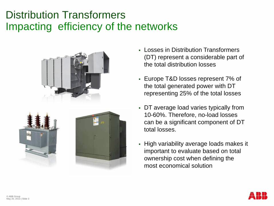
Distribution Transformers Impacting efficiency of the networks
Losses in Distribution Transformers (DT) represent a considerable part of the total distribution losses
Europe T&D losses represent 7% of the total generated power with DT representing 25% of the total losses
DT average load varies typically from 10-60%. Therefore, no-load losses can be a significant component of DT total losses.
High variability average loads makes it important to evaluate based on total ownership cost when defining the most economical solution
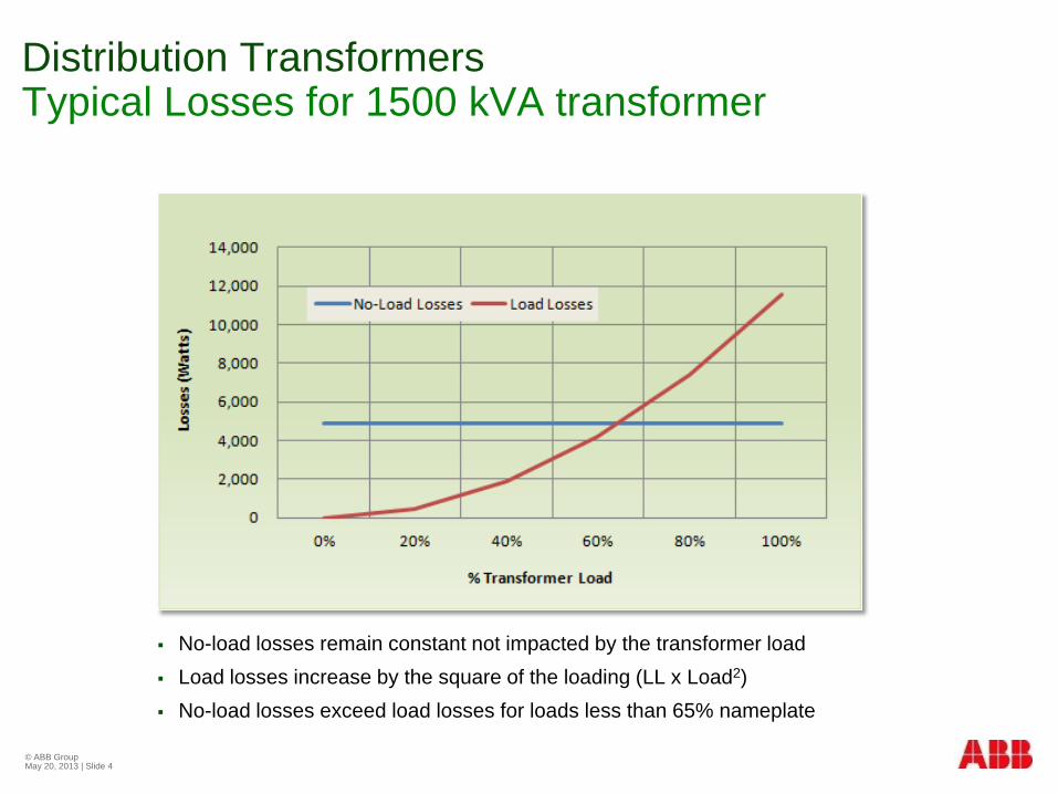
Distribution Transformers Typical Losses for 1500 kVA transformer
No-load losses remain constant not impacted by the transformer load Load losses increase by the square of the loading (LL x Load2) No-load losses exceed load losses for loads less than 65% nameplate
© ABB Group May 20, 2013 | Slide 4
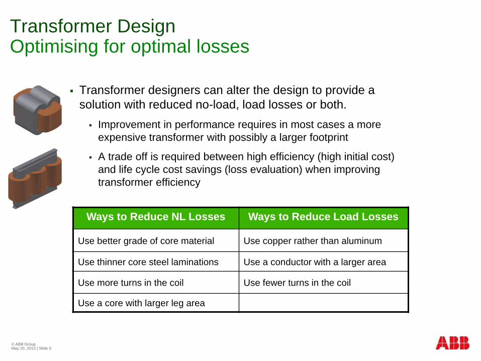
Transformer Design Optimising for optimal losses
Ways to Reduce NL Losses Ways to Reduce Load Losses
Use better grade of core material Use copper rather than aluminum
Use thinner core steel laminations Use a conductor with a larger area
Use more turns in the coil Use fewer turns in the coil
Use a core with larger leg area
© ABB Group May 20, 2013 | Slide 5
Transformer designers can alter the design to provide a solution with reduced no-load, load losses or both. Improvement in performance requires in most cases a more
expensive transformer with possibly a larger footprint
A trade off is required between high efficiency (high initial cost) and life cycle cost savings (loss evaluation) when improving transformer efficiency
© ABB Group May 20, 2013 | Slide 6
Total Ownership Cost Definition
© ABB 22/07/2009 | Slide 7
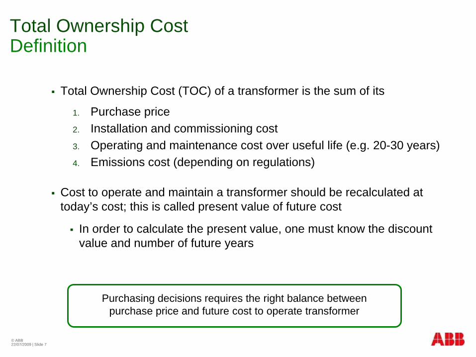
Total Ownership Cost Definition Total Ownership Cost (TOC) of a transformer is the sum of its
1. Purchase price 2. Installation and commissioning cost 3. Operating and maintenance cost over useful life (e.g. 20-30 years) 4. Emissions cost (depending on regulations)
Cost to operate and maintain a transformer should be recalculated at today’s cost; this is called present value of future cost
In order to calculate the present value, one must know the discount value and number of future years
Purchasing decisions requires the right balance between purchase price and future cost to operate transformer
© ABB 22/07/2009 | Slide 8
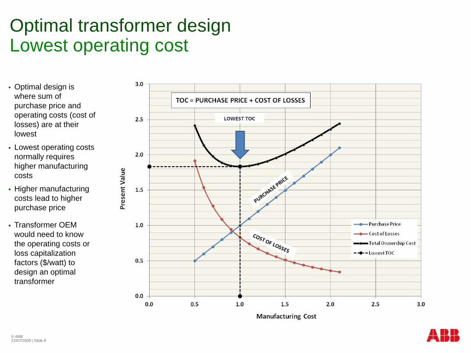
Optimal transformer design Lowest operating cost
Optimal design is where sum of purchase price and operating costs (cost of losses) are at their lowest
Lowest operating costs normally requires higher manufacturing costs
Higher manufacturing costs lead to higher purchase price
Transformer OEM would need to know the operating costs or loss capitalization factors ($/watt) to design an optimal transformer
© ABB Group May 20, 2013 | Slide 9
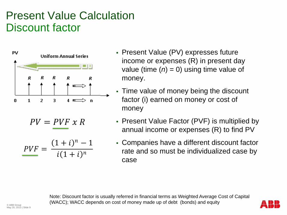
Present Value Calculation Discount factor
Present Value (PV) expresses future income or expenses (R) in present day value (time (n) = 0) using time value of money.
Time value of money being the discount factor (i) earned on money or cost of money
Present Value Factor (PVF) is multiplied by annual income or expenses (R) to find PV
Companies have a different discount factor rate and so must be individualized case by case
𝑃𝑃𝑃𝑃 = 𝑃𝑃𝑃𝑃𝑃𝑃 𝑥𝑥 𝑅𝑅
𝑃𝑃𝑃𝑃𝑃𝑃 = (1 + 𝑖𝑖)𝑛𝑛 − 1𝑖𝑖(1 + 𝑖𝑖)𝑛𝑛
Note: Discount factor is usually referred in financial terms as Weighted Average Cost of Capital (WACC); WACC depends on cost of money made up of debt (bonds) and equity

Present Value Calculation Time value of money
Your money is worth more today than in the future
Inflation reduces the purchasing power of future money relative to current ones
Overall uncertainty increases as one looks out further into the future.
The promise to pay 100 USD in 30 days is worth more than 100 USD in 90 days
Waiting to receive your money carries an opportunity cost associated with it as one is foregoing an opportunity to invest in the next best alternative
© ABB Group May 20, 2013 | Slide 10
Large discount rates reflect higher cost of capital and increased opportunity cost which results in lower present value factor

Present Value Calculation Time value of money
Discount factor (%) and project life (yrs) have an opposite impact on the present value factor
As discount factor increases it decreases the PVF
And as project life decreases it decreases the PVF
© ABB Group May 20, 2013 | Slide 11
Cost to operate transformers from a present value perspective becomes more expensive as useful life increases and as cost of money (% discount factor) becomes less
30 25 20 15 105.0% 15.37 14.09 12.46 10.38 7.726.0% 13.76 12.78 11.47 9.71 7.368.0% 11.26 10.67 9.82 8.56 6.7112.5% 7.77 7.58 7.24 6.63 5.5415.0% 6.57 6.46 6.26 5.85 5.0217.5% 5.67 5.61 5.49 5.21 4.5820.0% 4.98 4.95 4.87 4.68 4.19
PV FACTORS - Discount Factor (%) vs Project Life (yrs)
𝑃𝑃𝑃𝑃𝑃𝑃 = (1 + 𝑖𝑖)𝑛𝑛 − 1𝑖𝑖(1 + 𝑖𝑖)𝑛𝑛

© ABB Group May 20, 2013 | Slide 12
Net Present Value Example
𝑃𝑃𝑃𝑃 =(1 + 9%)8 − 19%(1 + 9%)8 𝑥𝑥 100 𝑈𝑈𝑈𝑈𝑈𝑈
NPV= -180 USD (570-750)
+30% Cost
CASE #1
CASE #2
2x Savings NPV Case #2 > Case #1
NPV= +121 USD (1096-975)
© ABB Group May 20, 2013 | Slide 13
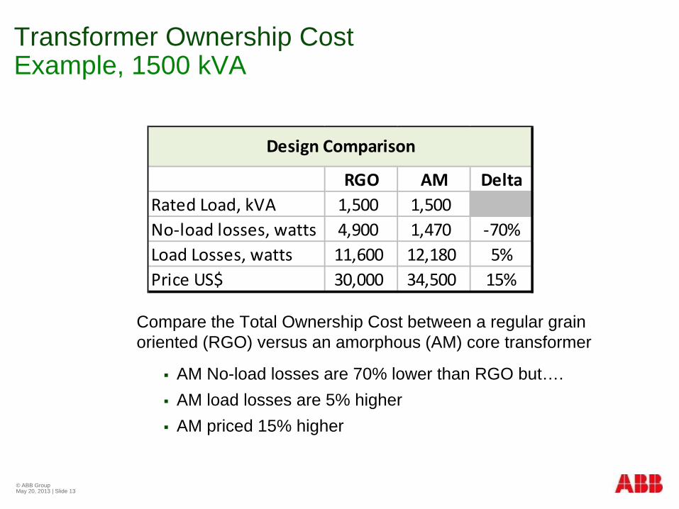
Transformer Ownership Cost Example, 1500 kVA
Compare the Total Ownership Cost between a regular grain oriented (RGO) versus an amorphous (AM) core transformer
AM No-load losses are 70% lower than RGO but…. AM load losses are 5% higher AM priced 15% higher
RGO AM DeltaRated Load, kVA 1,500 1,500No-load losses, watts 4,900 1,470 -70%Load Losses, watts 11,600 12,180 5%Price US$ 30,000 34,500 15%
Design Comparison
© ABB Group May 20, 2013 | Slide 14
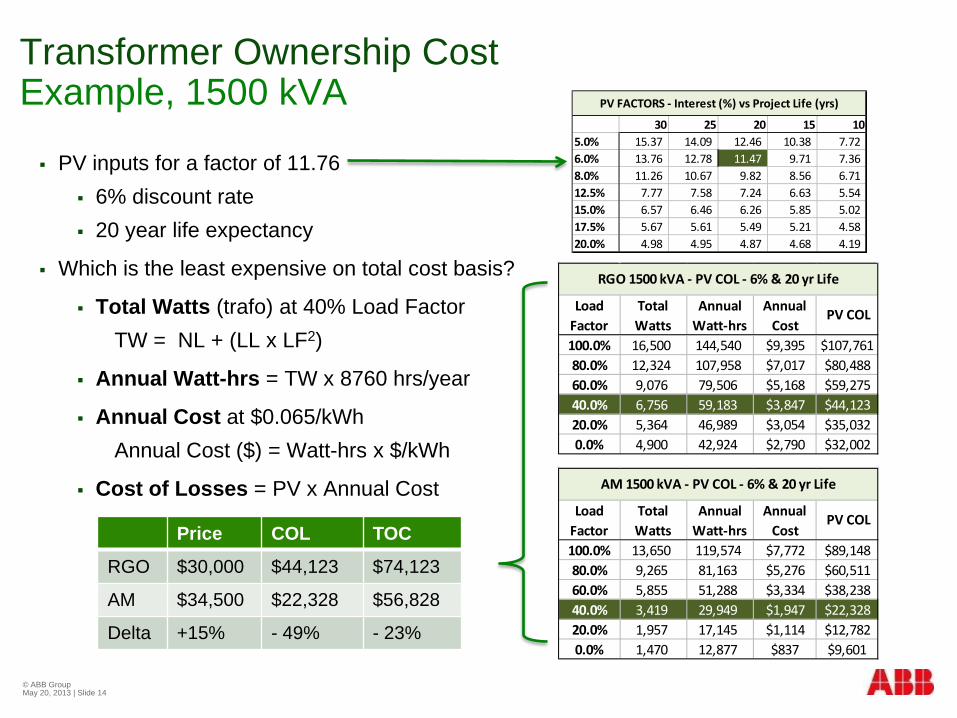
Transformer Ownership Cost Example, 1500 kVA
PV inputs for a factor of 11.76 6% discount rate 20 year life expectancy
Which is the least expensive on total cost basis?
Total Watts (trafo) at 40% Load Factor TW = NL + (LL x LF2)
Annual Watt-hrs = TW x 8760 hrs/year
Annual Cost at $0.065/kWh Annual Cost ($) = Watt-hrs x $/kWh
Cost of Losses = PV x Annual Cost
100.0% 16,500 144,540 $9,395 $107,76180.0% 12,324 107,958 $7,017 $80,48860.0% 9,076 79,506 $5,168 $59,27540.0% 6,756 59,183 $3,847 $44,12320.0% 5,364 46,989 $3,054 $35,0320.0% 4,900 42,924 $2,790 $32,002
RGO 1500 kVA - PV COL - 6% & 20 yr Life
Load Factor
Total Watts
Annual Watt-hrs
Annual Cost
PV COL
100.0% 13,650 119,574 $7,772 $89,14880.0% 9,265 81,163 $5,276 $60,51160.0% 5,855 51,288 $3,334 $38,23840.0% 3,419 29,949 $1,947 $22,32820.0% 1,957 17,145 $1,114 $12,7820.0% 1,470 12,877 $837 $9,601
Load Factor
Total Watts
Annual Watt-hrs
Annual Cost
PV COL
AM 1500 kVA - PV COL - 6% & 20 yr Life
Price COL TOC
RGO $30,000 $44,123 $74,123
AM $34,500 $22,328 $56,828
Delta +15% - 49% - 23%
30 25 20 15 105.0% 15.37 14.09 12.46 10.38 7.726.0% 13.76 12.78 11.47 9.71 7.368.0% 11.26 10.67 9.82 8.56 6.7112.5% 7.77 7.58 7.24 6.63 5.5415.0% 6.57 6.46 6.26 5.85 5.0217.5% 5.67 5.61 5.49 5.21 4.5820.0% 4.98 4.95 4.87 4.68 4.19
PV FACTORS - Interest (%) vs Project Life (yrs)
© ABB Group May 20, 2013 | Slide 15
Loss capitalization A & B factors
© ABB Group May 20, 2013 | Slide 16
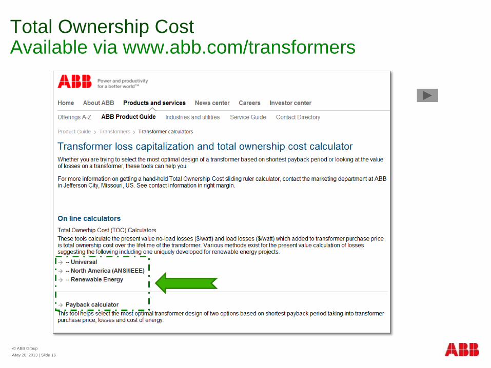
Total Ownership Cost Available via www.abb.com/transformers

Transformers Ownership Cost Universal calculator
© ABB Group May 20, 2013 | Slide 17
© ABB Group May 20, 2013 | Slide 18
Transformer Ownership Cost Cost of losses (COL)
Transformer future operating expenses are called Cost of Losses (COL)
COL is a function of no-load losses and load losses
Transformer designer seeks an optimal design between production cost and losses
For a utility customer, lower losses results in lower operating cost and deferral of generation, transmission and distribution capacity investments.
Cost of Losses ($) = (A x NLL) + (B x LL)
A ($/W) = present value (capitalization factor) cost of no-load losses
B ($/W) = present value (capitalization factor) cost of load losses
NLL (W) = transformer no-load losses
LL (W) = transformer load losses A & B Factors are unique to each purchaser of the transformer even to their
respective industry being residential, commercial, industrial and generation.
© ABB Group May 20, 2013 | Slide 19
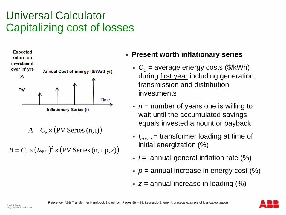
Universal Calculator Capitalizing cost of losses
Reference: ABB Transformer Handbook 3rd edition. Pages 88 – 98: Leonardo-Energy A practical example of loss capitalization
Present worth inflationary series
Ce = average energy costs ($/kWh) during first year including generation, transmission and distribution investments
n = number of years one is willing to wait until the accumulated savings equals invested amount or payback
Iequiv = transformer loading at time of initial energization (%)
i = annual general inflation rate (%)
p = annual increase in energy cost (%)
z = annual increase in loading (%)
PV
( )i)(n, Series PV×= eCA
( ) ( )z)p,i,(n, Series PV2 ××= equive ICB
© ABB Group May 20, 2013 | Slide 20
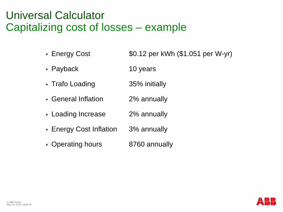
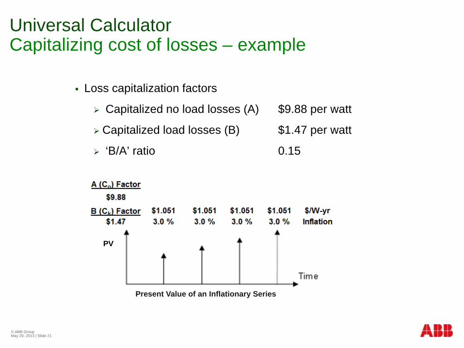
Universal Calculator Capitalizing cost of losses – example
Energy Cost $0.12 per kWh ($1.051 per W-yr)
Payback 10 years
Trafo Loading 35% initially
General Inflation 2% annually
Loading Increase 2% annually
Energy Cost Inflation 3% annually
Operating hours 8760 annually
© ABB Group May 20, 2013 | Slide 21
Loss capitalization factors
Capitalized no load losses (A) $9.88 per watt
Capitalized load losses (B) $1.47 per watt
‘B/A’ ratio 0.15
Universal Calculator Capitalizing cost of losses – example
PV
Present Value of an Inflationary Series
© ABB Group May 20, 2013 | Slide 22
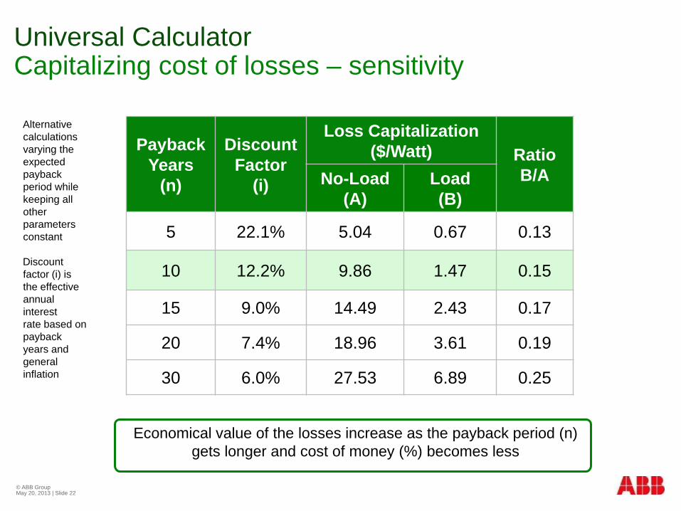
Universal Calculator Capitalizing cost of losses – sensitivity
Economical value of the losses increase as the payback period (n) gets longer and cost of money (%) becomes less
Alternative calculations varying the expected payback period while keeping all other parameters constant Discount factor (i) is the effective annual interest rate based on payback years and general inflation
Payback Years
(n)
Discount Factor
(i)
Loss Capitalization ($/Watt) Ratio
B/A No-Load (A)
Load (B)
5 22.1% 5.04 0.67 0.13
10 12.2% 9.86 1.47 0.15
15 9.0% 14.49 2.43 0.17
20 7.4% 18.96 3.61 0.19
30 6.0% 27.53 6.89 0.25

Cost of Emissions Included within the cost of energy (Ce)
Emissions are also a cost to be considered not only on environmental but also economic impact
Several nations have agreed on a market value for certain pollutants (USD/ton) in a ‘Cap and Trade’ arrangement
One can consider such economic costs within the TOC calculation by adding emissions costs (Cem) to the cost of energy (Ce) for a total cost of energy (CE) which would take the place of Ce in the previous equations.
Emissions cost (Cem) would be calculated by multiplying the emissions per electricity generated Ep (tons/Wh) by the market value of the pollutant Ec (USD/ton)
© ABB Group May 20, 2013 | Slide 23
emeE CCC +=
cpem EEC ×=
© ABB Group May 20, 2013 | Slide 24
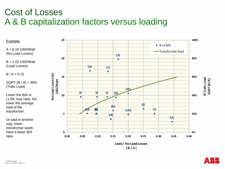
Cost of Losses A & B capitalization factors versus loading
Example: A = 8.10 USD/Watt (No Load Losses) B = 1.22 USD/Watt (Load Losses) B / A = 0.15 SQRT (B / A) = 39% (Trafo Load) Lower the B/A or LL/NL loss ratio, the lower the average load of the transformer. Or said in another way, lower transformer loads have a lower B/A ratio.
© ABB Group May 20, 2013 | Slide 25
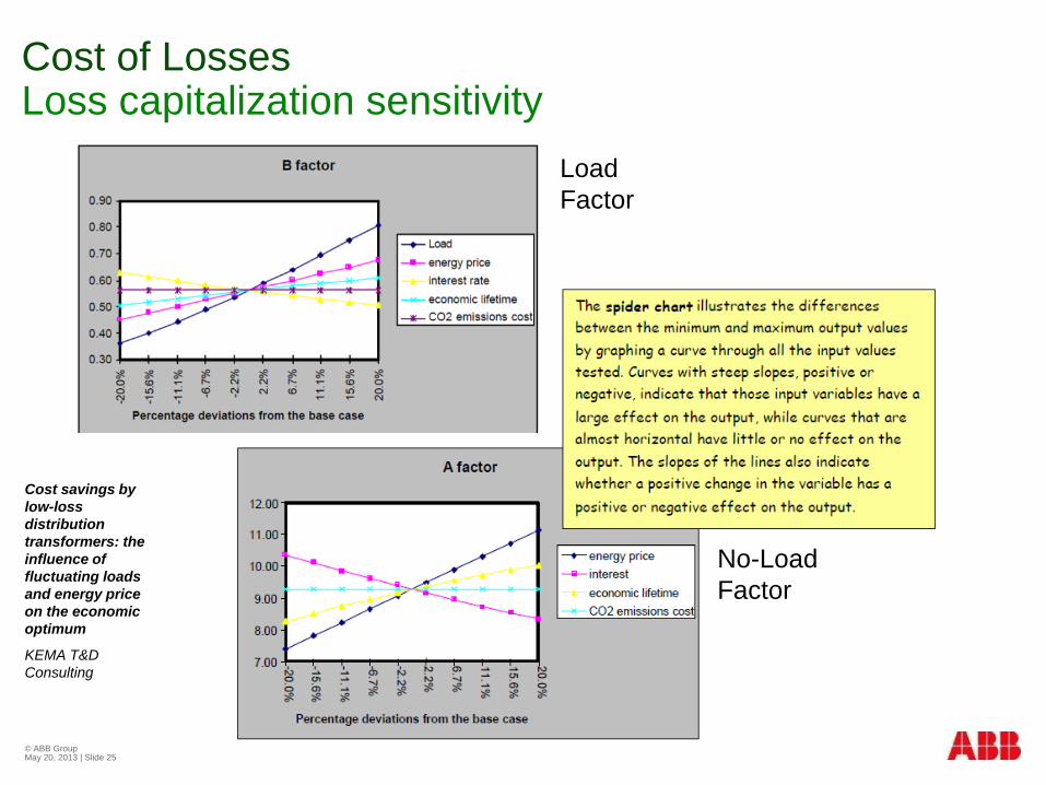
Cost of Losses Loss capitalization sensitivity
Cost savings by low-loss distribution transformers: the influence of fluctuating loads and energy price on the economic optimum
KEMA T&D Consulting
Load Factor
No-Load Factor

© ABB Group May 20, 2013 | Slide 26
Total Ownership Cost Payback period
© ABB Group May 20, 2013 | Slide 27
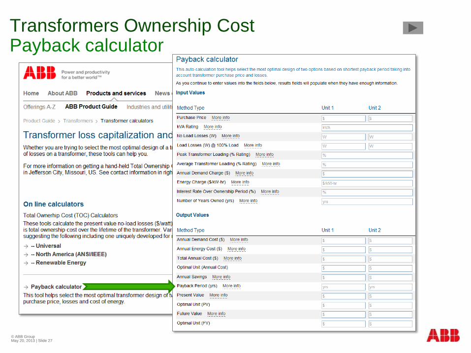
Transformers Ownership Cost Payback calculator
© ABB 22/07/2009 | Slide 28
Payback Period Definition
Payback period refers to the number of years a customers
would need to recover the additional investment (e.g. the
higher purchase price for a more efficient transformer) thanks
to the annual savings generated by having lower transformer
operating cost.
Purchasing decisions requires the right balance between
purchase price and future cost of losses.
© ABB Group May 20, 2013 | Slide 29
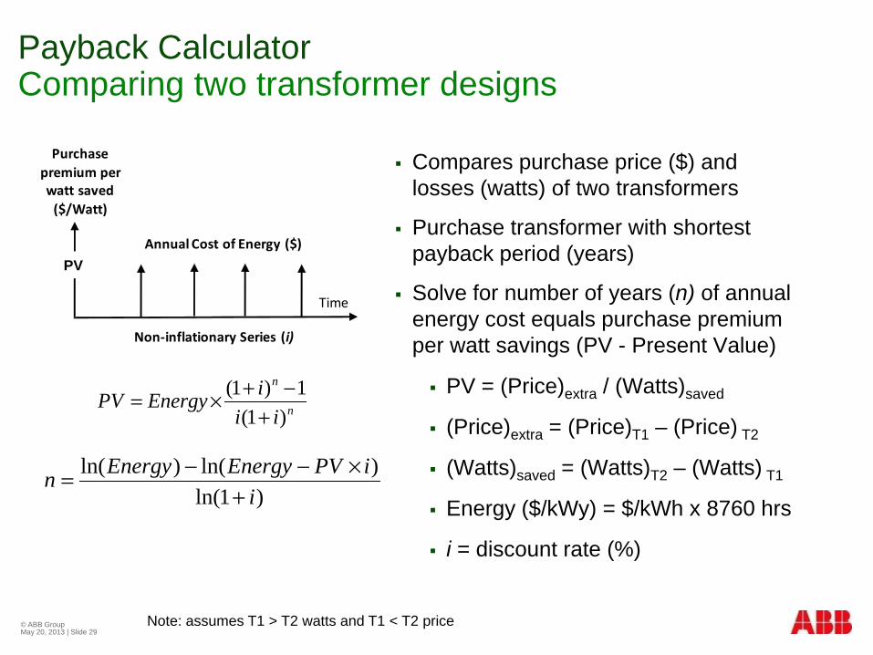
Payback Calculator Comparing two transformer designs
Compares purchase price ($) and losses (watts) of two transformers
Purchase transformer with shortest payback period (years)
Solve for number of years (n) of annual energy cost equals purchase premium per watt savings (PV - Present Value)
PV = (Price)extra / (Watts)saved
(Price)extra = (Price)T1 – (Price) T2
(Watts)saved = (Watts)T2 – (Watts) T1
Energy ($/kWy) = $/kWh x 8760 hrs
i = discount rate (%)
Time
Purchase premium per watt saved
($/Watt)
Annual Cost of Energy ($)
Non-inflationary Series (i)
PW
Note: assumes T1 > T2 watts and T1 < T2 price
n
n
iiiEnergyPV
)1(1)1(
+−+×=
)1ln()ln()ln(
iiPVEnergyEnergyn
+×−−=
PV
© ABB Group May 20, 2013 | Slide 30
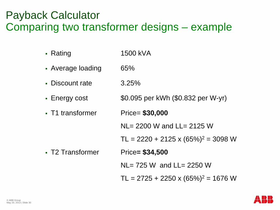
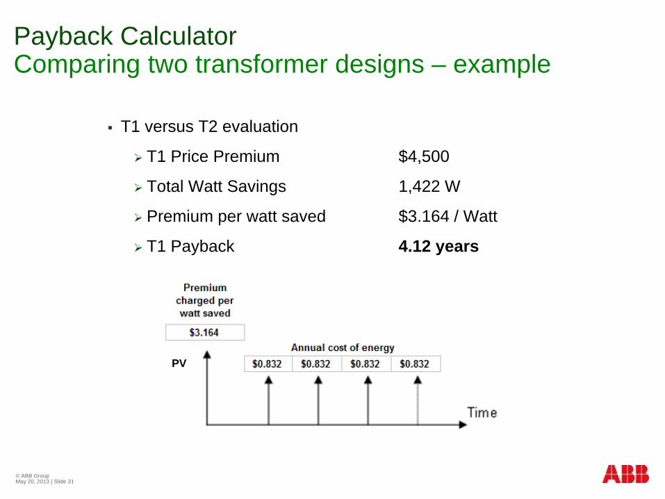
Payback Calculator Comparing two transformer designs – example
Rating 1500 kVA
Average loading 65%
Discount rate 3.25%
Energy cost $0.095 per kWh ($0.832 per W-yr)
T1 transformer Price= $30,000
NL= 2200 W and LL= 2125 W
TL = 2220 + 2125 x (65%)2 = 3098 W
T2 Transformer Price= $34,500
NL= 725 W and LL= 2250 W
TL = 2725 + 2250 x (65%)2 = 1676 W
© ABB Group May 20, 2013 | Slide 31
T1 versus T2 evaluation
T1 Price Premium $4,500
Total Watt Savings 1,422 W
Premium per watt saved $3.164 / Watt
T1 Payback 4.12 years
Payback Calculator Comparing two transformer designs – example
PV

© ABB Group May 20, 2013 | Slide 32
Case Study Renewable energy
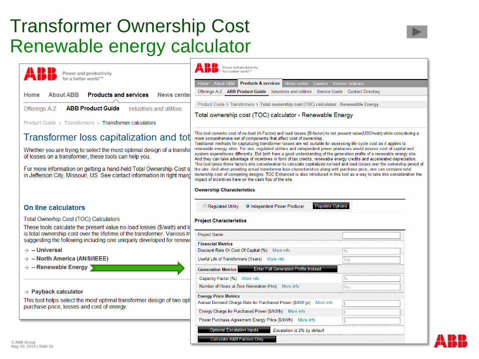
Transformer Ownership Cost Renewable energy calculator
© ABB Group May 20, 2013 | Slide 33
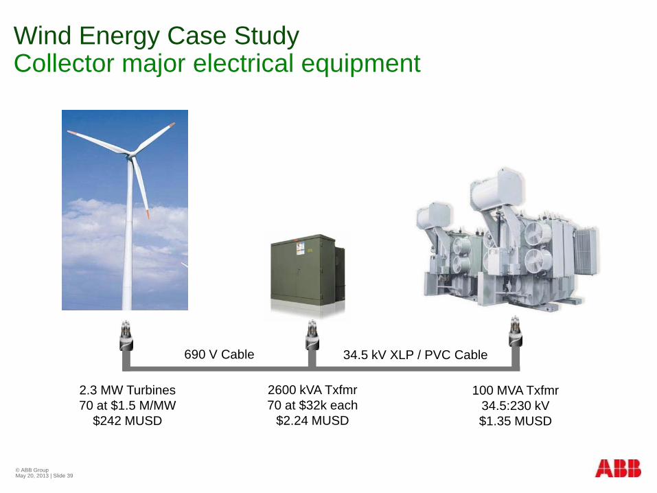
Wind Energy Case Study Collector major electrical equipment
© ABB Group May 20, 2013 | Slide 39
2.3 MW Turbines 70 at $1.5 M/MW
$242 MUSD
2600 kVA Txfmr 70 at $32k each
$2.24 MUSD
690 V Cable 34.5 kV XLP / PVC Cable
100 MVA Txfmr 34.5:230 kV $1.35 MUSD
© ABB Group May 20, 2013 | Slide 40
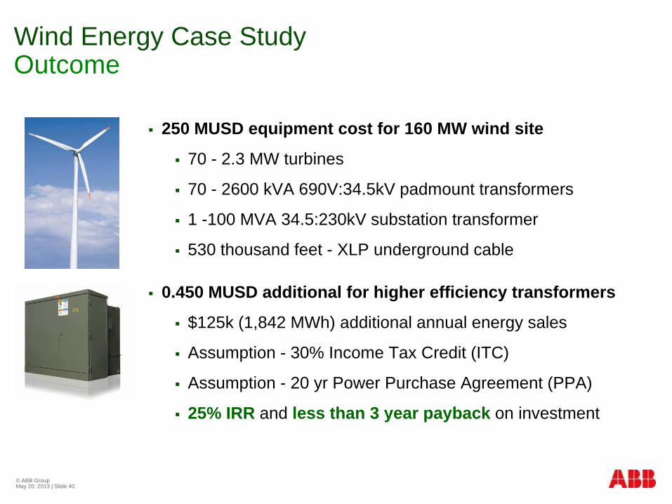
Wind Energy Case Study Outcome
250 MUSD equipment cost for 160 MW wind site
70 - 2.3 MW turbines
70 - 2600 kVA 690V:34.5kV padmount transformers
1 -100 MVA 34.5:230kV substation transformer
530 thousand feet - XLP underground cable
0.450 MUSD additional for higher efficiency transformers
$125k (1,842 MWh) additional annual energy sales
Assumption - 30% Income Tax Credit (ITC)
Assumption - 20 yr Power Purchase Agreement (PPA)
25% IRR and less than 3 year payback on investment
© ABB Group May 20, 2013 | Slide 41
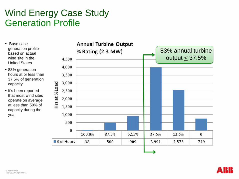
Wind Energy Case Study Generation Profile
Base case generation profile based on actual wind site in the United States
83% generation hours at or less than 37.5% of generation capacity
It’s been reported that most wind sites operate on average at less than 50% of capacity during the year
83% annual turbine output < 37.5%
© ABB Group May 20, 2013 | Slide 42
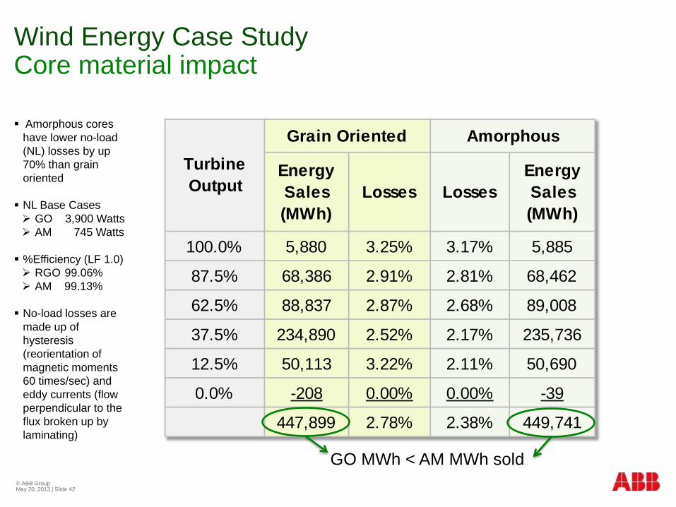
Wind Energy Case Study Core material impact
Amorphous cores have lower no-load (NL) losses by up 70% than grain oriented NL Base Cases GO 3,900 Watts AM 745 Watts %Efficiency (LF 1.0) RGO 99.06% AM 99.13% No-load losses are
made up of hysteresis (reorientation of magnetic moments 60 times/sec) and eddy currents (flow perpendicular to the flux broken up by laminating)
Energy Sales (MWh)
Losses LossesEnergy Sales (MWh)
100.0% 5,880 3.25% 3.17% 5,885
87.5% 68,386 2.91% 2.81% 68,462
62.5% 88,837 2.87% 2.68% 89,008
37.5% 234,890 2.52% 2.17% 235,736
12.5% 50,113 3.22% 2.11% 50,690
0.0% -208 0.00% 0.00% -39
447,899 2.78% 2.38% 449,741
Grain Oriented AmorphousTurbine Output
GO MWh < AM MWh sold
© ABB Group May 20, 2013 | Slide 43
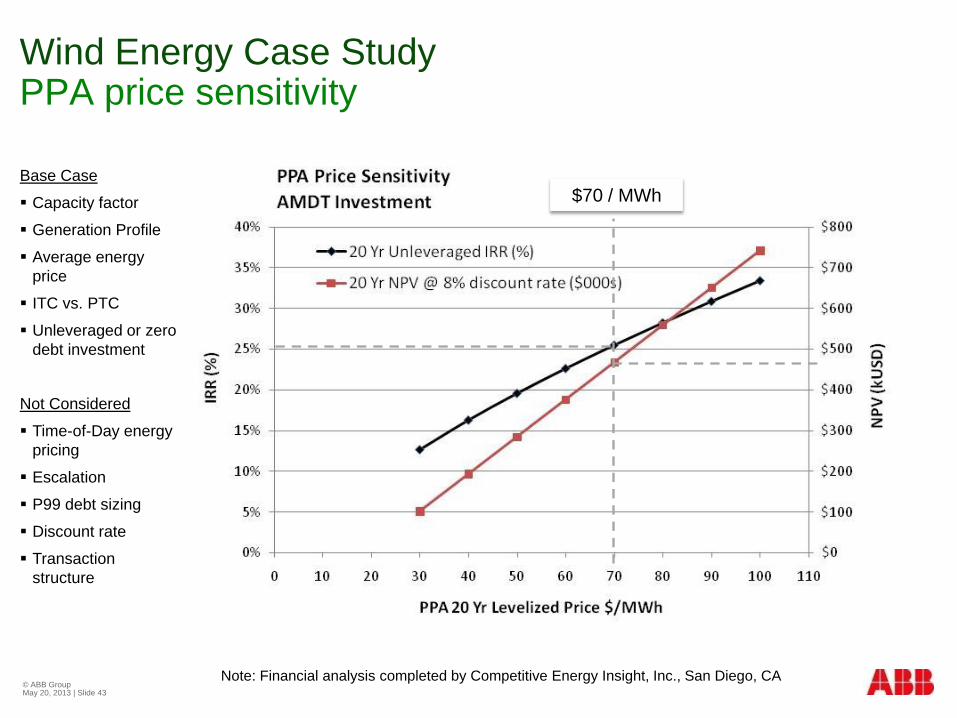
Wind Energy Case Study PPA price sensitivity
Base Case
Capacity factor
Generation Profile
Average energy price
ITC vs. PTC
Unleveraged or zero debt investment
Not Considered
Time-of-Day energy pricing
Escalation
P99 debt sizing
Discount rate
Transaction structure
$70 / MWh
Note: Financial analysis completed by Competitive Energy Insight, Inc., San Diego, CA

© ABB Group May 20, 2013 | Slide 44


