Downside Risk Portfolio DiversiÞcation Effects
Namwon Hyung and Casper G. de Vries∗
University of Seoul, Tinbergen Institute, and
Erasmus Universiteit Rotterdam
Febuary 2004
Abstract
Risk managers use portfolios to diversify away the unpriced risk of
individual securities. In this paper we compare the beneÞts of portfolio
diversiÞcation for downside risk with the variance. The risk of a secu-
rity is decomposed into a part which is attributable to the market risk
and an orthogonal risk factor. The orthogonal part consists of an id-
iosyncratic part and a part which is attributable to dependency between
assets, but which cannot be explained by the market risk. We Þnd that
the idiosyncratic downside risk evaporates more rapidly than the idiosyn-
cratic variance risk. For this we offer a theoretical explanation on basis
of the heavy tail properties of the asset return distributions. We also Þnd
that the non-diversiÞable non-market factors are more important for the
downside risk than for the global risk measure.
∗The Þrst author beneÞtted from a research grant of the Tinbergen Institute.
1

1 Introduction
Risk managers use portfolios to diversify away the unpriced risk of individual
securities. This topic has been well studied for global risk measures like the
variance, see e.g. the textbook by Elton and Gruber (1995, ch.4). In this
paper we study the beneÞts of portfolio diversiÞcation with respect to extreme
downside risk known as the zero-th lower partial moment (i.e. the inverse of the
VaR -Value at Risk- risk measure). The risk of a security is decomposed into a
part which is attributable to the market risk and an orthogonal risk factor. The
orthogonal part consists of an idiosyncratic part and a part which is attributable
to dependency between assets but which cannot be explained by the market risk,
i.e. there are other factors. Let the "diversiÞcation speed" denote the inverse
of the number of assets that have to be included into the portfolio in order to
eliminate the idiosyncratic parts of the orthogonal risk factors. We compare the
diversiÞcation speed of the downside risk measure with the diversiÞcation speed
regarding the variance. We Þnd that the idiosyncratic downside risk evaporates
at double the speed by which the idiosyncratic variance part disappears. For
this we offer a theoretical explanation on basis of the heavy tail properties of the
asset return distributions. We also Þnd that the non-diversiÞable non-market
factors are more important for the downside risk than for the global risk measure.
Furthermore, we provide predictions for the downside risk diversiÞcation beneÞts
beyond the range of the empirical distribution function.
The diversiÞcation speed of the variance risk measure for the idiosyncratic
risk part is equal to 1/n, where n is the number of securities (assuming the
2

idiosyncratic parts of the different securities have comparable variances). With
independent risks, the variance of the sum is just the sum of the variances,
regardless the distribution of the risks (provided the variance exists). The in-
tuition for the higher diversiÞcation speed of the downside risk measure is as
follows. For downside risk measures like the lower partial moments the tail
shape of the distribution is important, since the tail shape governs the upper
boundary of the integral. It is a well known fact that security returns are heavy
tail distributed, see e.g. Jansen and De Vries (1991). Thus the diversiÞcation
speed is dictated by the heavy tail property of the sum (by comparison, this
would be an exponential rate in case of the normal distribution). For a global
risk measure like the variance, the tail properties only play a role in the deter-
mination of the size of the variance of the individual random variable. But for
partial moments the sum operator enters the boundary of the integral. A sine
qua non for the existence of the variance is that the tail of the distribution must
go down at least at a quadratic speed. Thus the tail shape, even of the heavy
tail distributions, must be such that it beats the quadratic rate and hence the
higher diversiÞcation speed of the downside risk measure. For example, in case
of independent Student-t distributions with ν > 2 degrees of freedom, ensuring
the existence of the variance, the diversiÞcation speed of the downside risk mea-
sure equals 1/n1/(ν−1) (and hence exceeds the speed of the variance in all cases
for which the variance exists, i.e. if ν > 2). This intuition is made rigorous
below by means of the celebrated Feller convolution theorem for heavy tailed
(i.e. regularly varying) distributions.
3
For the empirical counterpart of this analysis, we brießy review the semi-
parametric approach to estimating the (extreme) downside risk. The heavy
tail feature is captured by a Pareto distribution like term, of which one needs to
estimate the tail index and scale coefficient. We consider estimation by means of
a pooled data set on basis of the assumption that the tail indices of the different
securities and risk components are equal. We do allow for heterogeneity of the
scale coefficients, though. Most securities� distributions display equal hyperbolic
tail coefficients, but do differ considerably in terms of their scale coefficients, see
Hyung and De Vries (2002). Within this framework it is possible to calculate
the diversiÞcation effects beyond the sample range and for hypothetically larger
portfolios, if we make some assumptions regarding the market model betas and
scale coefficients of the orthogonal risk factors.
We start our essay by reviewing the Feller�s convolution theorem for distri-
butions with heavy tails. Subsequently, we study the diversiÞcation problem
in more detail by adding the market factor. The relevance of the theoretical
results for the downside risk portfolio diversiÞcation question is demonstrated
by an application to S&P stock returns.
2 DiversiÞcation Effects and the Feller Convo-
lution Theorem
In this section we only consider securities which are independent and identically
distributed. In the next section this counterfactual assumption, as least as far as
4

equities are concerned, is relaxed by allowing for common factors. Let Ri denote
the logarithmic return of the i−th security. Suppose the {Ri} are generated by
a distribution with heavy tails in the sense of regular variation at inÞnity. Thus
far from the origin the Pareto term dominates:
Pr {Ri ≤ −x} = Aix−α[1 + o(1)], α > 0, Ai > 0, (1)
as x → ∞. The Pareto term implies that only moments up to α are bounded
and hence the informal terminology of heavy tails. Per contrast the normal
distribution has all moments bounded thanks to the exponential tail shape.
Distributions like the Student-t, Pareto, non-normal sum-stable distributions
all have regularly varying tails. Downside risk measures like the VaR directly
pick up differences in tail behavior. In this paper we focus on the loss probability
Pr {Ri ≤ −x} at high loss levels x as our measure of downside risk, rather than
at the loss level x as in case of the VaR measure.
An implication of the regular variation property is the simplicity of the tail
probabilities for convoluted data. Suppose the {Ri} are generated by a heavy-
tailed distribution which satisÞes (1). From the Feller�s Theorem (1971, VIII.8),
the distribution of the k−sum satisÞes
Pr
(kXi=1
Ri ≤ −x)
= kAx−α[1 + o(1)], as x→∞.
From this one can derive the diversiÞcation effect for the equally weighted port-
folio R = 1k
Pki=1Ri, see Dacorogna et al. (2001). The following Þrst order
5

approximation for the diversiÞcation effect regarding the downside risk obtains
Pr
(1
k
kXi=1
Ri ≤ −x)≈ k1−αAx−α. (2)
By comparison, if the variance would be used as the risk measure (assuming
α > 2), the portfolio has a variance which declines at a rate k only.
Under the heterogeneity of the scale coefficients Ai, the equivalent of equa-
tion (2) reads
Pr
(1
k
kXi=1
Ri ≤ −x)≈ k−α
ÃkXi=1
Ai
!x−α. (3)
At a constant VaR level x, increasing the number k of included securities
decreases the probability of loss by k1−α. If α > 2, then downside diversiÞca-
tion goes at a higher speed than if the returns would be normally distributed.
Hyung and De Vries (2002) investigate these diversiÞcation effects by means of
a simulation study and an application to portfolios with equities. This study
did not distinguish between different risk components and their contribution to
the downside risk. The following section extends the results to the case where
there are common and idiosyncratic risk factors.
3 DiversiÞcation Effects in Factor Models
We relax the assumption of independence between security returns and allow
for non-diversiÞable market risk. The market risk reduces the beneÞts from
6

diversiÞcation to the elimination of the idiosyncratic component of the risk.
First consider the single index model in which all risk which is orthogonal to
the market risk R is security speciÞc
Ri = βiR+Qi, (4)
where R, is the return on the market portfolio, βi is the amount of market
risk and Qi is the idiosyncratic risk of the return on asset i. The idiosyncratic
risk may be diversiÞed away fully in arbitrarily large portfolios and hence is
not priced. But the cross-sectional dependence induced by common market risk
factor has to be held in any portfolio.
We now apply Feller�s theorem again for deriving the beneÞts from cross-
sectional portfolio diversiÞcation in the single index model. Consider an equally
weighted portfolio of k assets. Let β = 1k
Pki=1 βi. The case of unequally
weighted portfolios is but a minor extension left to the reader for consideration
of space. In the single index model the Qi are cross-sectionally independent and
are independent from the market risk factor R. Suppose in addition that the
Qi satisfy Pr {Qi ≤ −x} ≈ Aix−α for all i, and that Pr {R ≤ −x} ≈ Arx
−α.
The diversiÞcation beneÞts from the equally weighted portfolio regarding the
downside risk measure for the case of homogenous scale coefficients Ai = A
then follow as
Pr
(1
k
kXi=1
Ri ≤ −x)≈ k1−αAx−α[1 + o(1)] + β
αArx
−α[1 + o(1)], (5)
7

as x→∞. If the scale coefficients are heterogenous, the equivalent of equation
(5) reads
Pr
(1
k
kXi=1
Ri ≤ −x)≈ k−α
ÃkXi=1
Ai
!x−α + β
αArx
−α . (6)
In arbitrarily large portfolios one should see that all downside risk is driven by
the market factor, if α > 1
Pr
(1
k
kXi=1
Ri ≤ −x)≈ βαArx−α
for large k.
In general one Þnds the single index model does not hold exactly due to the
fact that Cov[Qi, Qj ] is typically non-zero for off diagonal elements as well. Thus
though the Qi are uncorrelated with the market risk factor R by construction,
they are not cross sectionally independent from each other; moreover, one can
imagine they may not even be independent from R. This case is usually referred
to as the market model. For example, let there be one other common factor F .
This factor is uncorrelated with R, but the Cov[Qi, F ]/Cov[F,F ] = τi say. Let
τ = 1k
Pki=1 τi, and assume Pr {F ≤ −x} ≈ Afx−α. Then, by analogy with the
foregoing results
Pr
(1
k
kXi=1
Ri ≤ −x)≈ k−α
ÃkXi=1
Ai
!x−α + β
αArx
−α + ταAfx−α. (7)
8

4 Estimation by Pooling
To investigate the relevance of the above downside risk diversiÞcation theory, we
need to estimate the various downside risk components. To explain the details
of the estimation procedure, consider again the simple setup in (3). To be able
to calculate the downside risk measure, one needs estimates of the tail index
α and the scale coefficients Ai. A popular estimator for the inverse of the tail
index is Hill�s (1975) estimator. If the only source of heterogeneity are the scale
coefficients, one can pool all return series. Let {R11, ..., R1n, ..., Rk1, ..., Rkn} be
the sample of returns. Denote by Z(i) the i-th descending order statistic from
{R11, ..., R1n, ..., Rk1, ..., Rkn}. If we estimate the left tail of the distribution, it
is understood that we take the losses (reverse signs). The Hill estimator reads
d1/α =1
m
mXi=1
ln¡Z(i)
¢− ln¡Z(m+1)
¢. (8)
This estimator requires a choice of the number of the highest order statistics m
to be included, i.e. one needs to locate the start of the tail area. We imple-
mented the subsample bootstrap method proposed by Danielsson et al. (2000)
to determine m. The estimator for the scale A when A = Ai for all i is
bA =m
kn(Z(m+1))
bα.
Note that m/nk is the empirical probability associated with Z(m+1), and the
estimator bA follows intuitively from (1). Under the heterogeneity of Ai one
9

takes
bAi =mi
n(Z(m+1))
bα
where mi is such that
Ri(1) ≥ ... ≥ Ri(mi) ≥ Z(m+1) ≥ Ri(mi+1) ≥ ... ≥ Rin.
Note thatPki=1mi = m. This implies that by the pooling method we obtain
exactly the same portfolio probabilities whether or not one assumes (counter-
factually incorrect) identical or heterogenous scale coefficients, since
k−bα ÃkXi=1
bAi!x−bα = k−bα ÃkXi=1
mi
n(Z(m+1))
bα!x−bα
= k−bα³Pk
i=1mi
´n
(Z(m+1))bαx−bα
= k1−bα bAx−bα.
We can adapt this pooling method to the market model with little modiÞca-
tion. Pooling the series {R} , {Q1} , ... {Qk}, one can use the same procedure as
in the case of cross-independence.1 For the estimation of the tail index one uses
again (8), where in this case {Z} = {Rr1, ..., Rrn, Q11, ..., Q1n, ..., Qk1, ..., Qkn}.
1The determination of the parameters βi and the residuals Qi entering in the deÞnition ofthe market model is done by regressing the stock returns on the market return. The coefficientβi is thus given by the ordinary least squares estimator, which is consistent as long as theresiduals are white noise and have zero mean and Þnite variance. The idiosyncratic noise Qiis obtained by subtracting βi times the market return to the stock return.
10

Estimators for the scales are
bAi =mi
n(Z(m+1))
bα, i = 1, ..., k and r,
where mi is such that
Xi(1) ≥ ... ≥ Xi(mi) ≥ Z(m+1) ≥ Xi(mi+1) ≥ ... ≥ Xin,
where Xi can be R or Qi.
In case the tail indices differ across securities and risk factors, the above
can be easily adapted to estimation on individual series. There is however
considerable evidence that the tail indices are comparable for equities from the
S&P 500 index, see e.g. Jansen and De Vries (1991) and Hyung and De Vries
(2002). Therefore we decided to proceed on basis of the assumption that the
tail indices are equal.
5 Empirical Analysis of the DiversiÞcation Speed
We now apply our theoretical results to the daily returns of a set of stocks. In
order to estimate the parameters of the market model we choose the Standard
and Poor�s 500 index as a representation of the market factor. This is certainly
not the market portfolio as in the CAPM; nevertheless, the S&P 500 index
represents about 80% of the total market capitalization. To see the effects of
portfolio diversiÞcation, we choose arbitrarily 15 stocks from the S&P 100 index
11
in March of 2001. We use the daily returns (close-to-close data), including cash
dividends. The data were obtained from the Datastream. The data span runs
from January 2, 1980, through March 6, 2001, giving a sample size of n = 5,526.
Thus more than 20 years of daily data are considered, including the 1987 Crash.
All results are in terms of the excess returns above the risk free interest rate
(three month US Treasury bills).
The summary statistics for each stock return series and the market factor
are given in Table 1. On an annual basis the excess returns hover around
7.5% and have comparable second moments. The excess returns all exhibit
considerably higher than normal kurtosis. This latter feature is also captured
by the estimates of the tail index α in Table 2. In this table we report tail index
and scale estimates using the individual series, counter to the pooling method
outlined above. This is done in order to show that the tail indices are indeed
rather similar, while there is considerable variation in the scales. This motivates
the single tail index, heterogenous scale model implemented in the other tables.
Table 2 also gives the beta estimates for the market model.
In Table 3 computations proceed by using the pooling method, assuming
identical tail indices for all risk components. We report the estimates of the
scale parameter A, and the optimal number of order statistics m. Both are
calculated for the series of excess returns and for the (constructed) orthogonal
residuals from the market model (using the betas from Table 2). The tail index
estimate using all excess returns is 3.163, while when we use all the residuals the
tail index is 3.246. The scale parameter estimates, however, differ considerably
12

since these range between 14.4 and 46.4 for the excess returns, and are between
4.3 and 42.2 for the market returns and residuals respectively. We note that
the scale estimates for the excess returns using the pooling method are more
homogeneous than when using the individual series approach from Table 2.
The effects of portfolio diversiÞcation are reported in Table 4. The downside
risk measure is the probability of a loss in excess of the VaR level s; we report
at four different loss levels (respectively s =7.10, 11.69, 13.33 and 15.97). Four
different levels of portfolio aggregation are considered: one stock, 5 stocks, 10
stocks and 15 stocks. The numbers in row EMP are the probabilities from the
empirical distribution function of the total return series. The normal law is
often used as the workhorse distribution model in Þnance, even though it does
not capture the characteristic tail feature of the data. Therefore in the rows
labelled NOR we give the probabilities from the normal model based formula,
using the mean and variance estimates from the averaged series. The estimated
values in rows FAT were obtained by the heavy tail model using the averaged
total excess returnsPk
i=1Ri/k. The rows CDp give the probability estimates
from the pooled series on the basis of (6) assuming the heterogenous scale model.
One notes that the normal model does well in the center, but performs miserable
as one moves into the tail part. Per contrast, the averaged series in rows FAT
is always quite close to the empirical distribution function in the tail area. This
shows that the heavy tail model much better captures the tail properties. If we
turn to the last rows , one notes that the model in (6) does capture a considerable
part of the tail risk of the portfolio, but that there is a gap between the tail risk
13

0.00
0.01
0.02
0.03
0.04
0.05
1 2 3 4 5 6 7 8 9 10 11 12 13 14 15
prob
abili
ty
Market component Idiosyncratic component Total risk
Figure 1: Downside Risk Decomposition at s=-7.10
which is explained by the model and which is left unexplained. This is further
interpreted below.
To judge these results a graphical exposition is insightful. In Figures 1 and
2 we graph the downside risk (VaR probability levels) against the number of
securities which are included in the portfolio. Figure 1 is for the 7.10 VaR level,
and Figure 2 concerns the 15.97 VaR level. The top line gives the total amount
of tail risk by means of the empirical distribution function. The grey area consti-
tutes the market risk component, while the black area contains the idiosyncratic
risk part of the residual risk from model (6). Note that the idiosyncratic risk is
basically eliminated once the portfolio includes about seven stocks. To put this
result into perspective, we also provide a graph for the speed of diversiÞcation
concerning the variance, see Figure 3. As can be seen from this latter Þgure, it
14

0.0000
0.0005
0.0010
0.0015
0.0020
0.0025
0.0030
0.0035
0.0040
1 2 3 4 5 6 7 8 9 10 11 12 13 14 15
prob
abili
ty
Market component Idiosyncratic component Total risk
Figure 2: Downside Risk Decomposition at s=-15.97
0.0
5.0
10.0
15.0
20.0
25.0
1 2 3 4 5 6 7 8 9 10 11 12 13 14 15
Varia
nce
Variance of Market component Variance Idiosyncratic component Variance of Portfolio
Figure 3: Variance Decomposition
15

takes approximately double the number of securities to eliminate the variance
part contributed by the idiosyncratic risk part (which is consistent with the
value of the tail index), cf. Elton and Grubel (1995). Hence, the diversiÞcation
speed is higher for the downside risk measure. This corroborates the theoretical
predictions above. Interestingly as noted at the end of the previous paragraph,
another remarkable difference between the last Þgure and the Þrst two Þgures
is the size of the residual risk driven by the factors other than the market fac-
tor. While this component is relatively minor for the variance risk measure, it
is even larger than the market risk component for the downside risk measure.
This points to the presence of another factor F uncorrelated with R as in (7).
This other factor induces correlation between the residuals, see Figure 3. This
correlation is small but not negligible. But it the importance of this other factor
is really with respect to the downside risk. In future research we hope to relate
this factor to economic variables.
6 Out-of-sample, Out-of-portfolio
The semi-parametric approach we followed to construct the downside risk mea-
sure can also be used to go beyond the sample. We consider two possible
applications of this technique which might be of use to risk managers. The Þrst
application asks the question how much extra diversiÞcation beneÞts could be
derived from adding more securities, without having observations on these secu-
rities. By making an assumption regarding the value of the average beta and the
16

average scale of the residual risk factors in the enlarged portfolio, one can use
(6) to extrapolate to larger than sample size portfolios. A second application is
to increase the loss levels at which one wants to evaluate the downside risk level
beyond the worst case in sample. Moreover, even at the border of the sample
our approach has real beneÞts. By its very nature the empirical distribution is
bounded by the worst case and hence has its limitations, since the worst case
is a bad estimator of the quantile at the 1/n probability level (and vice versa).
Thus increasing the loss level x in (6) beyond the worst case gives an idea about
the risk of observing even higher losses.
In Table 5 the block denoted as Case I just summarizes some information
from the previous Table 4. The Case III block addresses the Þrst application
by increasing the number of securities k beyond the sample value of 15. We
assumed the following average beta values: β = 0.7, 0.83 and 0.9. The Case II
block increases the loss return level. In Table 4 we used 15.97 as the highest
loss level. Above this level many securities have no observations. There is one
equity with much higher loss returns and we used this one to provide the �out
of sample� loss levels of 22.03, 25.21, 33.69 and 40.45 respectively. To interpret
Case III, note that the inclusion of more stocks that have a close correlation
with the market component increases the loss probability for a given VaR level.
For example consider a portfolio of k = 30 stocks, at the -15.97 quantile when
β = 0.7 the probability is 0.0169 but when β = 0.9 the probability increases to
0.0381.
17

7 Conclusion
Risk managers use portfolios to diversify away the unpriced risk of individual
securities. In this paper we study the beneÞts of portfolio diversiÞcation with
respect to extreme downside risk, or the VaR (Value at Risk) risk measure.
The risk of a security is decomposed into a part which is attributable to the
market risk and an orthogonal risk factor. The orthogonal part consists of
an idiosyncratic part and a part which is attributable to dependency between
assets but which cannot be explained by the market risk, i.e there are other
factors. We compare the diversiÞcation speed of the downside risk measure with
the diversiÞcation speed regarding the variance and Þnd that the idiosyncratic
downside risk evaporates at a higher speed. For this we offer a theoretical
explanation on basis of the heavy tail properties of the asset return distributions.
We also Þnd that the non-diversiÞable non-market factors are more important
for the downside risk than for the global risk measure. Furthermore, we provide
predictions for the downside risk diversiÞcation beneÞts beyond the range of the
empirical distribution function.
This research can be extended in several directions. For theoretical reasons
as well for empirical reasons it is of interest to extend the analysis to portfolios
which include securities with heterogenous tail indices. Given the large gaps in
Figures 1 and 2 between the total downside risk and the market factor downside
risk contribution, it is of interest to see whether one can identify the remaining
risk factors F as in (7). Moreover, one would like to explain why these remaining
risk factors are relatively unimportant for the global risk measure.
18

References
[1] Dacorogna, M.M, U.A. Müller, O.V. Pictet and C.G. de Vries, 2001. Ex-
tremal forex returns in extremely large data sets, Extremes 4, 105-127.
[2] Danielsson, J., L. de Haan, L. Peng, and C.G. de Vries, 2000. Using a boot-
strap method to choose the sample fraction in tail index estimation, Journal
of Multivariate Analysis 76, 226-248.
[3] Elton, E.J. and M.J. Gruber,1995. Modern Portfolio Theory and Investment
Analysis, 5th ed., Wiley, NewYork.
[4] Feller, W., 1971. An Introduction to Probability Theory and Its Applications,
Vol. II, Wiley, New York.
[5] Hill, B.M., 1975. A simple general approach to inference about the tail of a
distribution, Annals of Statistics, 3(5), 1163-1173.
[6] Jansen, D. and C.G. De Vries 1991. On the frequency of large stock re-
turns: Putting booms and busts into perspective. Review of Economics and
Statistics, 73, 18-24.
[7] Hyung, N. and C.G. de Vries, 2002. Portfolio DiversiÞcation Effects and Reg-
ular Variation in Financial Data, Allgemeines Statistisches Archiv/Journal
of the German Statistical Society 86, 69-82.
19

Table 1. Selected Stocks and Summary Statistics of Excess returns
Series Name µ1 µ2 µ3 µ4
m S&P 500 Index .0747 2.52 -2.31 55.491 ALCOA .0707 4.84 -0.26 13.392 AT & T .0392 4.33 -0.35 16.413 BLACK & DECKER -.0168 5.61 -0.32 10.574 CAMPBELL SOUP .0897 4.37 0.28 9.065 DISNEY (WALT) .0981 4.86 -1.30 29.826 ENTERGY .0454 4.06 -0.97 23.667 GEN.DYNAMICS .0764 4.53 0.26 10.248 HEINZ HJ .0968 3.99 0.11 6.359 JOHNSON & JOHNSON .1053 4.08 -0.32 9.4510 MERCK .1212 3.96 -0.03 6.3111 PEPSICO .1170 4.43 -0.04 7.8212 RALSTON PURINA .1077 4.08 0.70 15.4113 SEARS ROEBUCK .0542 4.91 -0.24 16.8314 UNITED TECHNOLOGIES .0851 4.19 -0.10 6.8315 XEROX -.0423 5.48 -1.78 33.74
Note: Observations cover 01/01/1980 - 03/06/2001, giving 5526 daily observa-tions. The µ1, µ2, µ3 and µ4 denote the sample mean, standard error, skew-ness and kurtosis of annualized excess returns, respectively. The estimates arereported in terms of the excess returns above the risk free interest rate (USTreasury bill 3 months).
20

Table 2. Left Tail Parameter Estimates and Beta
Series α A m βRm 2.963 2.522 298 11 3.789 110.117 113 0.8772 2.785 7.953 289 0.9293 3.220 58.601 136 0.9384 3.505 48.766 68 0.7195 2.549 6.211 496 1.0126 1.981 1.339 682 0.4757 3.218 27.687 140 0.7108 3.404 25.811 197 0.6409 3.377 23.663 292 0.92710 4.035 104.724 62 0.85411 3.789 103.171 71 0.86712 3.136 14.106 190 0.66913 3.166 28.244 256 1.07414 4.335 288.036 66 0.89515 2.098 2.999 537 0.949
Note: The values in α,A,m, and β are respectively the tail index, the scaleparameter, the estimated optimal number of order statistics and market modelbeta.
21

Table 3. Left Tail Parameter Estimates
Excess returns ResidualsSeries A m A mT 23.0 16.3 19.6 1021Rm - - 4.3 151 26.2 122 24.7 862 19.5 91 15.2 533 46.4 216 42.2 1474 22.7 106 19.5 685 24.0 112 22.1 776 14.4 67 14.9 527 25.3 118 25.0 878 16.3 76 14.9 529 13.9 65 10.6 3710 15.7 73 11.5 4011 24.2 113 18.7 6512 15.0 70 16.4 5713 29.0 135 17.5 6114 20.2 94 13.2 4615 32.4 151 26.7 93
Note: The values in row T give estimates from the pooled series imposingscale homogeneity. The values in rows Rm, 1, 2, ..., 15 give estimates for themarket returns and the individual stock series for the total excess returns andthe residual parts. The values in columns A and m are the scale parameter andthe estimated optimal number of order statistics imposing identical tail indices.
22

Table 4. Lower Tail Probabilities in Percentages
s -7.10 -11.69k 1 5 10 15 1 5 10 15
EMP 4.995 1.195 0.633 0.579 0.995 0.253 0.145 0.145NOR 7.325 0.934 0.225 0.198 0.817 0.005 0.000 0.000FAT 6.551 1.181 0.741 0.706 0.988 0.265 0.185 0.171CDp - 0.633 0.392 0.423 - 0.125 0.078 0.084
s -13.33 -15.97k 1 5 10 15 1 5 10 15
EMP 0.489 0.163 0.109 0.127 0.235 0.109 0.090 0.090NOR 0.309 0.000 0.000 0.000 0.051 0.000 0.000 0.000FAT 0.603 0.179 0.129 0.118 0.304 0.104 0.078 0.071CDp - 0.082 0.051 0.055 - 0.046 0.028 0.030
Note: The entries in rows EMP are the probabilities from the empirical distri-bution. The rows NOR and FAT report the probabilities calculated directlyfrom the parameters of the averaged series itself, where in the former case oneuses the presumption of normality and in the latter case regular variation isimposed. The numbers in rows CDp are the probabilities estimated using thepooled series. The k denotes the number of individual stocks included in theaveraged series, and s is the loss quantile. Note probabilities are written inpercentage format.
23
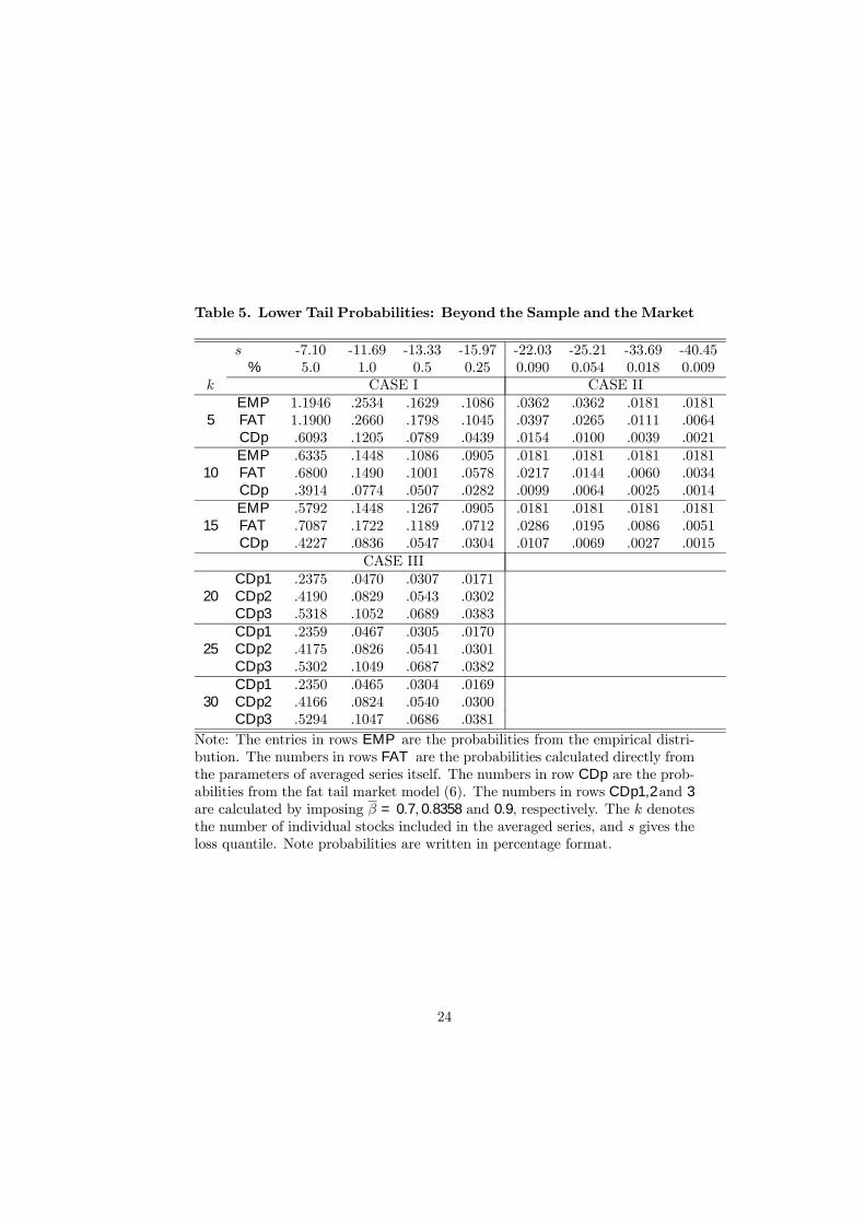
Table 5. Lower Tail Probabilities: Beyond the Sample and the Market
s -7.10 -11.69 -13.33 -15.97 -22.03 -25.21 -33.69 -40.45% 5.0 1.0 0.5 0.25 0.090 0.054 0.018 0.009
k CASE I CASE IIEMP 1.1946 .2534 .1629 .1086 .0362 .0362 .0181 .0181
5 FAT 1.1900 .2660 .1798 .1045 .0397 .0265 .0111 .0064CDp .6093 .1205 .0789 .0439 .0154 .0100 .0039 .0021EMP .6335 .1448 .1086 .0905 .0181 .0181 .0181 .0181
10 FAT .6800 .1490 .1001 .0578 .0217 .0144 .0060 .0034CDp .3914 .0774 .0507 .0282 .0099 .0064 .0025 .0014EMP .5792 .1448 .1267 .0905 .0181 .0181 .0181 .0181
15 FAT .7087 .1722 .1189 .0712 .0286 .0195 .0086 .0051CDp .4227 .0836 .0547 .0304 .0107 .0069 .0027 .0015
CASE IIICDp1 .2375 .0470 .0307 .0171
20 CDp2 .4190 .0829 .0543 .0302CDp3 .5318 .1052 .0689 .0383CDp1 .2359 .0467 .0305 .0170
25 CDp2 .4175 .0826 .0541 .0301CDp3 .5302 .1049 .0687 .0382CDp1 .2350 .0465 .0304 .0169
30 CDp2 .4166 .0824 .0540 .0300CDp3 .5294 .1047 .0686 .0381
Note: The entries in rows EMP are the probabilities from the empirical distri-bution. The numbers in rows FAT are the probabilities calculated directly fromthe parameters of averaged series itself. The numbers in row CDp are the prob-abilities from the fat tail market model (6). The numbers in rows CDp1,2and 3are calculated by imposing β = 0.7, 0.8358 and 0.9, respectively. The k denotesthe number of individual stocks included in the averaged series, and s gives theloss quantile. Note probabilities are written in percentage format.
24


