
. . . . . .
1
Dynamic Pricing and Inventory Managementunder Fluctuating Procurement Costs
Philip (Renyu) Zhang
(Joint work with Guang Xiao and Nan Yang)
Olin Business SchoolWashington University in St. Louis
June 20, 2014

. . . . . .
2
Motivation
Inventory management: To mitigate the demand uncertainty risk.
Current global market: Prices of many commodities are now fluctuatingas much in a single day as they did in a year in the early 1990s (Wigginsand Blas 2008).
. . . . . .
2
Motivation
Inventory management: To mitigate the demand uncertainty risk.
Current global market: Prices of many commodities are now fluctuatingas much in a single day as they did in a year in the early 1990s (Wigginsand Blas 2008).

. . . . . .
2
Motivation
Inventory management: To mitigate the demand uncertainty risk.
Current global market: Prices of many commodities are now fluctuatingas much in a single day as they did in a year in the early 1990s (Wigginsand Blas 2008).

. . . . . .
3
Motivation (Cont’d)
I Dynamic Pricing: Dynamically adjust the sales price in each period.
1. Demand control effect.
2. Risk-pooling effect.
I Dual-Sourcing: spot purchasing + forward-buying.
1. Cost-responsiveness tradeoff: differentiated costs and leadtimes.
2. Portfolio effect among different sourcing channels.
I Goal of our paper: To understand how to coordinate the dynamicpricing and dual-sourcing strategies to hedge against demanduncertainty and procurement cost fluctuation risks.

. . . . . .
4
Research Questions
1. What is the impact of procurement cost volatility?
2. How to optimally respond to the cost fluctuation?
3. How does the dual-sourcing flexibility affect the optimal policy?
4. What is the relationship between dynamic pricing and dual-sourcing?
. . . . . .
4
Research Questions
1. What is the impact of procurement cost volatility?
2. How to optimally respond to the cost fluctuation?
3. How does the dual-sourcing flexibility affect the optimal policy?
4. What is the relationship between dynamic pricing and dual-sourcing?

. . . . . .
4
Research Questions
1. What is the impact of procurement cost volatility?
2. How to optimally respond to the cost fluctuation?
3. How does the dual-sourcing flexibility affect the optimal policy?
4. What is the relationship between dynamic pricing and dual-sourcing?

. . . . . .
4
Research Questions
1. What is the impact of procurement cost volatility?
2. How to optimally respond to the cost fluctuation?
3. How does the dual-sourcing flexibility affect the optimal policy?
4. What is the relationship between dynamic pricing and dual-sourcing?

. . . . . .
5
Outline
I Related Literature
I Model
I Impact of Cost Volatility
I Impact of Dual-Sourcing
I Conclusion: Takeaway Insights

. . . . . .
6
Literature Review
I Inventory management under fluctuating costs:I Kalymon (1971),I Berling and Martınez-de-Albeniz (2011),I Chen et al. (2013).
I Joint price&inventory control:I Federgruen and Heching (1999),I Zhou and Chao (2014).
I Our paper: Joint pricing & inventory management under demanduncertainty, cost fluctuation, and dual-sourcing.

. . . . . .
7
Model Formulation: Basics
I A risk-neutral firm modeled as a T−period stochastic inventorysystem, labeled backwards, with discount factor α ∈ (0, 1).
I Maximize the total expected profit over the planning horizon.
I Endogenous pricing.
I Dual-sourcing:I Spot market: immediate delivery, fluctuating cost ct .
I Forward-buying contract: postponed delivery, with unit cost Ft(ct).

. . . . . .
8
Sequence of Events
I The firm reviews inventory It and spot market price ct .
I The firm makes the following decisions:I xt − It ≥ 0: spot-purchasing, delivered immediately;
I qt ≥ 0: forward-buying, delivered at the beginning of the next period;
I pt ∈ [p, p]: sales price in the customer market.
I Demand Dt(pt) realized, revenue collected.
I Net inventory fully carried over to the next period:I Excess inventory fully carried over with unit cost h;
I Unsatisfied demand fully backlogged with unit cost b.
. . . . . .
9
Demand Model
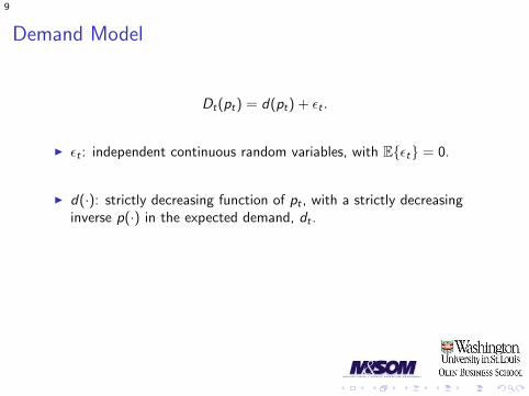
Dt(pt) = d(pt) + ϵt .
I ϵt : independent continuous random variables, with E{ϵt} = 0.
I d(·): strictly decreasing function of pt , with a strictly decreasinginverse p(·) in the expected demand, dt .
I We use dt = d(pt) ∈ [d , d ] as the decision variable.
Assumption 1
R(dt) := p(dt)dt is continuously differentiable and strictly concave.

. . . . . .
9
Demand Model
Dt(pt) = d(pt) + ϵt .
I ϵt : independent continuous random variables, with E{ϵt} = 0.
I d(·): strictly decreasing function of pt , with a strictly decreasinginverse p(·) in the expected demand, dt .
I We use dt = d(pt) ∈ [d , d ] as the decision variable.
Assumption 1
R(dt) := p(dt)dt is continuously differentiable and strictly concave.
. . . . . .
10
Spot-Market Price Fluctuation
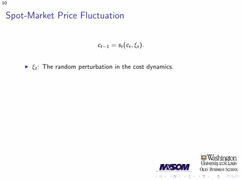
ct−1 = st(ct , ξt).
I ξt : The random perturbation in the cost dynamics.
I st(·, ·) > 0 a.s., and st(ct , ξt) ≥s.d. st(ct , ξt) for any ct > ct .
I µt(ct) := E{st(ct , ξt)} < +∞ is increasing in ct .I Perfect market: µt(ct) = ct/α.
I Examples: GBMs, mean-reverting processes.
I Inventory resale is not allowed: no room for arbitrage.

. . . . . .
10
Spot-Market Price Fluctuation
ct−1 = st(ct , ξt).
I ξt : The random perturbation in the cost dynamics.
I st(·, ·) > 0 a.s., and st(ct , ξt) ≥s.d. st(ct , ξt) for any ct > ct .
I µt(ct) := E{st(ct , ξt)} < +∞ is increasing in ct .I Perfect market: µt(ct) = ct/α.
I Examples: GBMs, mean-reverting processes.
I Inventory resale is not allowed: no room for arbitrage.

. . . . . .
11
Forward-Buying Contract
I To mitigate cost volatility at the expense of responsiveness.
I Forward-buying contract: (ft , qt):I The firm pays ftqt to the supplier in period te ;I The supplier delivers qt to the firm in period te ;I For technical tractability, te = t − 1.
I ft = γct/α.I Effective unit cost: γct .I Perfect market: γ = 1.I In general, ft is determined through bilateral negotiations.I Most results hold for general ft = Ft(ct).
I Focus on the operational effect of forward-buying.I The contract cannot be traded in the derivatives market.

. . . . . .
12
Bellman Equation
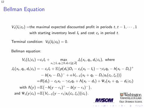
Vt(It |ct) =the maximal expected discounted profit in periods t, t − 1, · · · , 1with starting inventory level It and cost ct in period t.
Terminal condition: V0(I0|c0) = 0.
Bellman equation:
Vt(It |ct) =ct It + maxxt≥It ,qt≥0,dt∈[d,d ]
Jt(xt , qt , dt |ct), where
Jt(xt , qt , dt |ct) =− ct It + E{p(dt)Dt − ct(xt − It)− γctqt − h(xt − Dt)+
− b(xt − Dt)− + αVt−1(xt + qt − Dt |st(ct , ξt))}
=R(dt)− ctxt − γctqt + Λ(xt − dt) + Ψt(xt + qt − dt |ct)with Λ(y) =E{−h(y − ϵt)
+ − b(y − ϵt)−},
and Ψt(y |ct) =E{Vt−1(y − ϵt |st(ct , ξt))|ct}.
. . . . . .
12
Bellman Equation
Vt(It |ct) =the maximal expected discounted profit in periods t, t − 1, · · · , 1with starting inventory level It and cost ct in period t.
Terminal condition: V0(I0|c0) = 0.
Bellman equation:
Vt(It |ct) =ct It + maxxt≥It ,qt≥0,dt∈[d,d ]
Jt(xt , qt , dt |ct), where
Jt(xt , qt , dt |ct) =− ct It + E{p(dt)Dt − ct(xt − It)− γctqt − h(xt − Dt)+
− b(xt − Dt)− + αVt−1(xt + qt − Dt |st(ct , ξt))}
=R(dt)− ctxt − γctqt + Λ(xt − dt) + Ψt(xt + qt − dt |ct)with Λ(y) =E{−h(y − ϵt)
+ − b(y − ϵt)−},
and Ψt(y |ct) =E{Vt−1(y − ϵt |st(ct , ξt))|ct}.

. . . . . .
13
Optimal Policy
I (x∗t (It , ct), q∗t (It , ct), d
∗t (It , ct)): the optimal decisions in period t.
I ∆∗t (It , ct) := x∗
t (It , ct)− d∗t (It , ct): the optimal safety stock.
I The cost-dependent order-up-to/pre-order-up-to list-price policy.
I If It ≤ xt(ct), order from both channels and charge a list price.
I If It ∈ [xt(ct), I∗t (ct)], order via the forward-buying contract only and
charge a discounted price.
I If It ≥ I ∗t (ct), order nothing and charge a discounted price.

. . . . . .
14
Impact of Cost Volatility
I Higher demand variability −→ lower profit.
I Surprisingly, the prediction is reversed for cost volatility.
Theorem 1
For two procurement cost processes {ct}1t=T and {ct}1t=T , assume thatfor every t = T ,T − 1, · · · , 1, st(ct , ξt) and st(ct , ξt) are concavelyincreasing in ct for any realization of ξt . The following statements hold:
(a) Vt(It |ct) is convexly decreasing in ct , for any It .(b) If {ct}1t=T and {ct}1t=T are identical except that
sτ (cτ , ξτ ) ≥cx sτ (cτ , ξτ ) for some cτ and τ , Vt(It |ct) ≥ Vt(It |ct) foreach (It , ct) and t, where ≥cx refers to larger in convex order, and{Vt(It |ct)}1t=T are the value functions associated with {ct}1t=T .

. . . . . .
15
Impact of Cost Volatility (Cont’d)
I Higher cost volatility −→ higher profit.
I The fundamental difference between demand and cost risks:I Demand risk: decisions made prior to demand realization.
I Betting on demand uncertainty.
I Cost risk: decisions made posterior to cost realization.
I Responding to cost volatility.
I The impact of decision timing with respect to uncertainty realizationin capacity management and newsvendor network models withresponsive/postponed pricing: Van Mieghem and Dada (1999),Chod and Rudi (2005) and Bish et al. (2012).

. . . . . .
16
Impact of Cost Volatility: Assumptions
I Risk neutrality is necessary for Theorem 1 to hold.
I The concavity of st(ct , ξt) generally can be satisfied (e.g., GBMs,mean-reverting processes).
I When st(ct , ξt) is not concave in ct , the result holds for the majorityof numerical cases (except when the initial cost is low), in particularwhen the initial cost follows the stationary distribution.
. . . . . .
17
Optimal Response to Cost Volatility
I Optimal sales price: d∗t (It , ct) ↓ ct , i.e., p
∗t (It , ct) ↑ ct . The firm
passes (part of) the cost risk to customers.
Jt(xt , qt , dt |ct) =[R(dt)− ctdt ] + [Λ(∆t)− (1− γ)ct∆t ]
+ [Ψt(∆t + qt |ct)− γct(∆t + qt)].
I Three objectives: (a) generating revenue, (b) hedging againstdemand uncertainty, and (c) speculating on future costs.
I Optimal safety-stock and spot-purchasing: ∆t(ct), xt(ct) ↓ ct , ifγ ≤ 1; ∆t(ct) ↑ ct , if γ > 1.
I Optimal forward-buying quantity: generally not monotone in ct .
I Higher future cost trend −→ d∗t (It , ct) ↓, x∗t (It , ct) ↑, ∆∗
t (It , ct) ↑,and q∗t (It , ct) ↑.

. . . . . .
18
Impact of Dual-Sourcing Flexibility
I γ: the cost ratio between forward-buying and spot-purchasing.Lower γ implies higher dual-sourcing flexibility.
I Intuition suggests q∗t (It , ct) ↓ γ.Due to procurement costfluctuation, this may not be true in general:
I γ ↓ −→ d∗t (It , ct) ↑, x∗
t (It , ct) ↓, ∆∗t (It , ct) ↓.
I q∗t (It , ct) may not be monotone in γ, because lower γ also decreases
the marginal value of inventory in future periods.
I When γ is big enough (γ ≥ sup{αµt(ct)ct
}), the model is reduced toone with sole-sourcing from spot market alone.
I Dual-sourcing −→ d∗t (It , ct) ↑, x∗
t (It , ct) ↓, ∆∗t (It , ct) ↓ (Zhou and
Chao, 2014).

. . . . . .
18
Impact of Dual-Sourcing Flexibility
I γ: the cost ratio between forward-buying and spot-purchasing.Lower γ implies higher dual-sourcing flexibility.
I Intuition suggests q∗t (It , ct) ↓ γ.
Due to procurement costfluctuation, this may not be true in general:
I γ ↓ −→ d∗t (It , ct) ↑, x∗
t (It , ct) ↓, ∆∗t (It , ct) ↓.
I q∗t (It , ct) may not be monotone in γ, because lower γ also decreases
the marginal value of inventory in future periods.
I When γ is big enough (γ ≥ sup{αµt(ct)ct
}), the model is reduced toone with sole-sourcing from spot market alone.
I Dual-sourcing −→ d∗t (It , ct) ↑, x∗
t (It , ct) ↓, ∆∗t (It , ct) ↓ (Zhou and
Chao, 2014).

. . . . . .
18
Impact of Dual-Sourcing Flexibility
I γ: the cost ratio between forward-buying and spot-purchasing.Lower γ implies higher dual-sourcing flexibility.
I Intuition suggests q∗t (It , ct) ↓ γ.Due to procurement costfluctuation, this may not be true in general:
I γ ↓ −→ d∗t (It , ct) ↑, x∗
t (It , ct) ↓, ∆∗t (It , ct) ↓.
I q∗t (It , ct) may not be monotone in γ, because lower γ also decreases
the marginal value of inventory in future periods.
I When γ is big enough (γ ≥ sup{αµt(ct)ct
}), the model is reduced toone with sole-sourcing from spot market alone.
I Dual-sourcing −→ d∗t (It , ct) ↑, x∗
t (It , ct) ↓, ∆∗t (It , ct) ↓ (Zhou and
Chao, 2014).

. . . . . .
18
Impact of Dual-Sourcing Flexibility
I γ: the cost ratio between forward-buying and spot-purchasing.Lower γ implies higher dual-sourcing flexibility.
I Intuition suggests q∗t (It , ct) ↓ γ.Due to procurement costfluctuation, this may not be true in general:
I γ ↓ −→ d∗t (It , ct) ↑, x∗
t (It , ct) ↓, ∆∗t (It , ct) ↓.
I q∗t (It , ct) may not be monotone in γ, because lower γ also decreases
the marginal value of inventory in future periods.
I When γ is big enough (γ ≥ sup{αµt(ct)ct
}), the model is reduced toone with sole-sourcing from spot market alone.
I Dual-sourcing −→ d∗t (It , ct) ↑, x∗
t (It , ct) ↓, ∆∗t (It , ct) ↓ (Zhou and
Chao, 2014).

. . . . . .
19
Value of Dynamic Pricing and Dual-sourcing
I Dynamic pricing and dual-sourcing are strategic complements, i.e.,the application of one strategy increases the value of the other.
I When sourcing from the less responsive forward-buying channel, theflexibility to control demand via pricing becomes more valuable.
I In Zhou and Chao (2014), they are strategic substitutes.
I Compared with Zhou and Chao (2014), cost volatility renders thevalue of dynamic pricing and dual-sourcing significantly higher.

. . . . . .
20
Conclusion: Takeaway Insights
I A risk-neutral firm benefits from the procurement cost volatility.I Timing of decision making and uncertainty realization.
I Dynamic pricing and dual-sourcing are strategic complements.I Dynamic pricing dampens both demand and cost risks, while
dual-sourcing mitigates the cost risk but intensifies the demand risk.
. . . . . .
20
Conclusion: Takeaway Insights
I A risk-neutral firm benefits from the procurement cost volatility.
I Timing of decision making and uncertainty realization.
I Dynamic pricing and dual-sourcing are strategic complements.I Dynamic pricing dampens both demand and cost risks, while
dual-sourcing mitigates the cost risk but intensifies the demand risk.

. . . . . .
20
Conclusion: Takeaway Insights
I A risk-neutral firm benefits from the procurement cost volatility.I Timing of decision making and uncertainty realization.
I Dynamic pricing and dual-sourcing are strategic complements.I Dynamic pricing dampens both demand and cost risks, while
dual-sourcing mitigates the cost risk but intensifies the demand risk.

. . . . . .
20
Conclusion: Takeaway Insights
I A risk-neutral firm benefits from the procurement cost volatility.I Timing of decision making and uncertainty realization.
I Dynamic pricing and dual-sourcing are strategic complements.
I Dynamic pricing dampens both demand and cost risks, whiledual-sourcing mitigates the cost risk but intensifies the demand risk.

. . . . . .
20
Conclusion: Takeaway Insights
I A risk-neutral firm benefits from the procurement cost volatility.I Timing of decision making and uncertainty realization.
I Dynamic pricing and dual-sourcing are strategic complements.I Dynamic pricing dampens both demand and cost risks, while
dual-sourcing mitigates the cost risk but intensifies the demand risk.

. . . . . .
21
Q&A
Thank you!
Questions?


