Download - Economic Catastrophe Bonds: Ine cient Market or Inadequate ... Catastrophe... · Economic Catastrophe Bonds: Ine cient Market or Inadequate Model? ABSTRACT In an in uential paper,

Economic Catastrophe Bonds: Ine�cient Market or InadequateModel?

Haitao Lia and Feng Zhaob

ABSTRACT

In an in uential paper, Coval, Jurek and Sta�ord (2009, CJS hereafter) argue that senior CDX

tranches resemble economic catastrophe bonds|\bonds that default only under severe economic

conditions." Using a Merton structural model within a CAPM framework, CJS argue that senior

CDX tranches are overpriced relative to S&P 500 index options and therefore do not su�ciently

compensate investors for their inherent economic catastrophe risks. In this paper, we argue

that the conclusion of CJS that senior CDX tranches are overpriced is premature. We provide

compelling evidence that the CJS model is not exible enough to capture CDX tranches prices.

On the other hand, we develop a simple model that can simultaneously price CDX tranches and

index options. Our results show that the CDX tranches market is actually e�cient.

JEL Classi�cation: C11, E43, G11

Keywords: CDX index and tranches, copula model, economic catastrophe risk, fat tail.

aStephen M. Ross School of Business, University of Michigan, Ann Arbor, MI 48109, email: [email protected].

bSchool of Management, University of Texas at Dallas, Richardson, TX 75080, email: [email protected]. We

thank Ren-raw Chen, Pierre Collin-Dufresne, Robert Goldstein, and Robert Jarrow for helpful comments. We are

responsible for any remaining errors.

Economic Catastrophe Bonds: Ine�cient Market or Inadequate

Model?

ABSTRACT

In an in uential paper, Coval, Jurek and Sta�ord (2009, CJS hereafter) argue that senior CDX


conditions." Using a Merton structural model within a CAPM framework, CJS argue that senior

CDX tranches are overpriced relative to S&P 500 index options and therefore do not su�ciently

compensate investors for their inherent economic catastrophe risks. In this paper, we argue

that the conclusion of CJS that senior CDX tranches are overpriced is premature. We provide

compelling evidence that the CJS model is not exible enough to capture CDX tranches prices.

On the other hand, we develop a simple model that can simultaneously price CDX tranches and

index options. Our results show that the CDX tranches market is actually e�cient.

JEL Classi�cation: C11, E43, G11

Keywords: CDX index and tranches, copula model, economic catastrophe risk, fat tail.

1 Introduction

The fast growing credit derivatives markets have made it much easier to invest in the credit risk

of portfolios of companies. One of the most widely traded multi-name credit derivatives is the

standardized North American Investment Grade Credit Default Swap Index (CDX.NA.IG), an

equally-weighted portfolio of 125 liquid credit default swap (CDS) contracts on U.S. companies

with corporate debts above investment grade. Investors frequently use the CDX index to hedge

a portfolio of bonds or to take positions on a basket of credit entities to speculate on changes

in credit quality. CDX tranches, derivative securities with payo�s based on the losses on the

underlying CDX index, are also widely used by investors who desire di�erent risk and return

properties than the CDX index.1 For example, even though the underlying collaterals might have

low credit ratings, senior CDX tranches can have AAA rating due to the seniority of their cash

ow rights.

One of the key challenges in both �nancial industry and academics is the pricing of CDX

tranches, which depends crucially on the correlation of defaults of the underlying collaterals. The

�nancial industry has relied heavily on the copula model of Li (2002) in setting the price of CDX

tranches and other collateralized debt obligations (CDOs). The widespread adoption of the copula

model is partly due to its ease of implementation. For example, in the Gaussian copula model of

Li (2002), given the marginal probability of default of each individual �rm, one can easily obtain

the joint default probability distribution through the Gaussian copula and the prices of CDX

tranches in closed-form.

The copula model, however, has several well recognized limitations. First, the parameters

of the copula model do not have clear economic meanings. For example, it is rather di�cult

1CDX tranches are de�ned in terms of their loss attachment points. The 0-3, 3-7, 7-10, 10-15, and 15-30 tranches

are the most popular ones in the market.

1

to relate the parameters of the copula model to standard measures of credit risk, such as asset

beta, market volatility, and leverage ratio. Second, the standard Gaussian copula model cannot

satisfactorily capture CDX tranches prices, as evidenced by the so-called \correlation skew," the

fact that di�erent copula correlation parameters are needed to �t di�erent tranches. This is a

clear sign of model misspeci�cation because if the copula model is correctly speci�ed, then the

copula correlation should be the same for all CDO tranches. Finally, though various extensions

to the Gaussian copula model have been proposed to capture the \correlation skew," without a

clear economic underpinning these extensions appear to be ad hoc and might over�t the data.

In an in uential paper, Coval, Jurek and Sta�ord (2009) develop a structural model for pricing

CDX tranches. They explicitly model the capital structure of a �rm and assume that default

happens if the �rm asset value hits some exogenous default boundaries as in Merton (1974). While

standard structural models do not explicitly distinguish between systematic and idiosyncratic

risks, the CJS model assumes that the �rm asset return follows the CAPM and that defaults

of di�erent �rms are correlated due to their exposures to the same systematic factor. Though

structural models have clear economic meaning, their implementations are much more complicated

than that of the copula model. They tend to have a large number of parameters, require data from

other markets, and lack the analytical tractability of the copula model. CJS argue that senior CDX


conditions." CJS show that while their model can jointly price S&P 500 index options and CDX

index, it cannot capture the prices of CDX tranches. They conclude that senior CDX tranches are

overpriced and do not su�ciently compensate investors for the economic catastrophe risks they

bear.

While CJS interpret their results as evidence of mispricing of economic catastrophe risks

embedded in CDX tranches, it could also be evidence that either the CJS model is misspeci�ed

2

or the markets of equity, index option, CDX index and tranches are not well integrated. In this

paper, we re-examine the pricing of CDX tranches using the same data under the same modeling

framework of CJS. We believe this is a very important issue in both economics and �nance for

several reasons.

First, the CDX index is one of the most liquid credit derivatives, even more liquid than

most single-name CDS contracts. Many investors reply on CDX tranches to extract market

expectations on default correlation for hedging or speculation purpose. Mispriced CDX tranches

could easily lead to biased expectations and sub-optimal investment decisions. Second, as pointed

by Collin-Dufresne, Goldstein, and Yang (2010, CGY hereafter), \traders in the CDX market

are typically thought of as being rather sophisticated. Thus, it would be surprising to �nd them

accepting so much risk without fair compensation." Finally, recent papers by Longsta� and Rajan

(2008), Azizpour and Giesecke (2008), and Eckner (2008) �nd that CDX index and tranches are

consistently priced under reduced-form models, and conclude that these securities are reasonably

e�ciently priced. If CDX tranches are mis-priced, then it would imply some of these reduced-form

models, especially models based on the top-down approach, would be invalid, because they reply

on accurate CDX tranches prices to calibrate model parameters.

We �rst show that the structural approach has a simpli�ed representation as the standard

copula model. In particular, we show that the copula correlation measures the fraction of the total

variance of �rm asset return due to the systematic factor under the structural approach. We refer

to this fraction as the variance ratio for the rest of the paper. Our observation greatly simpli�es

the implementations of structural models: If we interpret the copula correlation as the variance

ratio, then the structural approach can be implemented in similar ways as the copula model.

Since the copula correlation measures the variance ratio, it should depend on the same factors

that drive the beta and the systematic and idiosyncratic volatilities. Moreover, since the betas of

3

most companies tend to increase and the relative importance of the systematic and idiosyncratic

volatilities tend to change during crisis, our approach suggests that the copula correlation should

be time varying to capture reality. Therefore, in our paper we implement structural models in the

same way as the copula model with time varying correlation. Our method shares the advantages

of both approaches and at the same time avoids their shortcomings.

We then provide a detailed analysis on the limitations of both the implementations and the

structure of the CJS model. The CJS model has several important ingredients. First, they cali-

brate the beta and volatility of the idiosyncratic factor by matching the average beta and pairwise

correlation of observed equity returns of 125 �rms underlying the CDX index. Second, they as-

sume the idiosyncratic factor follows a Gaussian distribution. Third, they allow the systematic

factor to follow a skewed distribution and back it out from prices of S&P 500 index options.

We show empirically that each of the three ingredients could lead to signi�cant pricing errors of

CDX tranches. We �rst show that the way CJS calibrate the beta and volatility of the idiosyncratic

factor introduces signi�cant biases in CDX tranche prices. Following the same procedure as CJS

and using their model parameters, we obtain huge pricing errors of the CDX tranches: The

RMSE of percentage pricing errors for �ve year CDX tranches is 1,584.%! On the other hand, if

we implement the CJS model as a copula model and estimate the copula correlation from prices

of CDX tranches, we obtain much smaller pricing errors of the CDX tranches: The RMSE of

percentage pricing errors is 50%. For the purpose of pricing CDX tranches, all we need is the

variance ratio but not the individual components of the systematic and idiosyncratic volatility.

Therefore, the copula approach is more e�cient than the structural approach, which has to

estimate the individual components of the total variance. Moreover, the pricing of CDX tranches

requires the variance ratio under the risk-neutral measure, whereas the estimates in the CJS paper

are under the physical measure. Finally, the CJS approach relies on the extra assumption that

4

the equity market is integrated with the credit market.

We then show that the Gaussian distribution of the idiosyncratic factor under the CJS model

could also introduce signi�cant biases in CDX tranches prices. CJS argue that it is reasonable

to assume that the idiosyncratic factor follows a Gaussian distribution because it describes the

conditional return given the systematic factor. However, we show that an idiosyncratic factor that

follows fat-tailed distribution leads to signi�cantly smaller pricing errors for CDX tranches. In

our copula implementation of the CJS model with a Gaussian idiosyncratic factor, the RMSE of

percentage pricing error is 50%. However, if we allow the idiosyncratic factor to follow a Student-

t distribution with degree of freedom of 3, the RMSE is reduced to about 33%. This result is

consistent with that of CGY (2010) who show under a structural model with stochastic volatility

and jumps, it is important to introduce jumps in the dynamics of idiosyncratic factor to price

CDX tranches.

Finally, we show that the functional form CJS use to back out the distribution of the systematic

factor from index options is not exible enough to capture CDX tranches prices. CJS obtain (i)

the distribution of the systematic factor from index option prices and (ii) the idiosyncratic factor

and debt equity ratio from individual equity prices and CDX index spreads. Then they price

CDX tranches based on these calibrated parameters. In some sense, they are doing an out-of-

sample analysis, using a model calibrated from index option and CDX index markets to price

CDX tranches. Since their model can price index options and CDX index jointly but not CDX

tranches, they argue that the CDX tranches are mis-priced. We show, however, that the CJS

model is so in exible that it cannot even capture the CDX tranches prices in sample! Speci�cally,

we retain the functional form of the systematic factor in the CJS model, but instead of calibrating

the parameters from index option prices, we obtain the parameters by directly �tting the CDX

tranches prices. We also calibrate the copula correlation from CDX tranches prices and maintain

5

a Gaussian idiosyncratic factor. Even though the model is �tted using in sample data, the RMSE

of percentage pricing errors is still as high as 45%.

Collectively, our analysis demonstrates from three di�erent aspects the limitations of the CJS

model. Therefore, the conclusion of CJS that the CDX tranches are overpriced seems to be

premature. Since market e�ciency tests are always a joint test of e�cient market and good

model, it is really di�cult to draw any inference on market e�ciency based on a model that

cannot even capture the CDX tranches prices in sample. A more reasonable conclusion seems to

be that the CJS model is probably misspeci�ed. To determine whether CDX tranches are fairly

priced, we still need to answer the question whether any model can simultaneously price index

options and CDX tranches. Despite the fact that the CJS model is misspeci�ed, if we cannot �nd

a model that can jointly price index options and CDX tranches, then there is still the possibility

that either the two markets are not well integrated or one of them is not e�cient.

We develop a simple copula model that can jointly price index options and CDX tranches very

well. We obtain our model by simply modifying the distributional assumptions of the systematic

and idiosyncratic factors of the CJS model. CJS back out the systematic factor from index option

prices based on a speci�c functional form and assume the idiosyncratic factor follows Gaussian

distribution. In contrast, we allow both the systematic and idiosyncratic factors to follow Student-

t distribution in one version of our model. It has been widely recognized that fat tails in both the

systematic and idiosyncratic factors are needed to capture CDX tranches prices. The �rst version

of the model is simply the double-t model of Hull and White (2004). Due to the volatility skew for

index options, we also consider a skewed-t model, in which the systematic factor follows a skewed-t

distribution of Hansen (1994) and the idiosyncratic factor follows the Student-t distribution.

We implement our model following the copula approach. Instead of separately modelling the

systematic and idiosyncratic volatilities as in CJS, we focus on the variance ratio, or the copula

6

correlation, which is crucial for pricing CDX tranches. Following the approach of CJS, we assume

that all the underlying �rms of CDX index are homogeneous with the same default probability.

We back out the marginal probability of default from the CDX index. As a result our model

perfectly �ts the CDX index by design. Taking the marginal probability of default as an input,

we price the CDX tranches based on our model. Following the daily calibration approach of CJS,

we choose the copula correlation and the degree of freedom of the Student-t distribution of both

factors to minimize the daily percentage pricing errors of index options and CDX tranches at �ve

year maturity, thus allowing all three important parameters to be time varying.2

Our empirical results show that our model can capture the daily prices of the index options

and CDX tranches very well. The estimated parameters show that the copula correlation and the

degrees of freedom need to vary dramatically over time to capture CDX tranches prices. When we

�t the double-t model to prices of CDX tranches, we obtain average RMSE of about 7.5% for �ve

year CDX tranches. When we �t the double-t model to prices of both CDX tranches and index

options, we obtain average RMSE of about 7.7% for CDX tranches and 7.8% for index options.

The double-t model cannot fully capture the volatility skew of index options. Finally, we �t the

skewed-t model to prices of both CDX tranches and index options. We obtain average RMSE of

about 7.85% for CDX tranches and 0.96% for index options. Hence, the skewed-t distribution is

needed mainly for pricing index options.

We emphasize that the structure of our model is almost exactly the same as that of CJS. The

only di�erences are the distributional assumptions of the systematic and idiosyncratic factors

and the way we calibrate the copula correlation. Though the CJS model has huge pricing errors

2Intuitively, time-varying systematic tail risk can change the value of a portfolio even there is no change in the

loss distribution. For portfolios with zero exposures to the systematic factor, time-varying idiosyncratic tail risk

can a�ect their values without changing the loss distribution.

7

for CDX tranches, our model can price both CDX tranches and index options very well. We

model both factors using Student-t distribution for convenience. There are many other fat-tailed

distributions we can use, which could lead to potentially even smaller pricing errors. Therefore,

the fact that the simple changes we make to the CJS model can lead to such dramatic di�erences

in pricing performance is a strong indication that the conclusion of CJS that CDX tranches are

mispriced is not a robust result.

Our analysis complements the important paper of CGY (2010), who also study the relative

pricing of index options and CDX tranches. They develop a structural model with stochastic

volatility, stochastic dividend yield, and correlated jumps in market return, volatility and dividend

yield, and show that the model can price index options and CDX tranches reasonably well. Our

model di�ers from the CGY model in several important ways. First, since our model stays strictly

within the framework of the CJS model, it is easier to compare the two models and to understand

the limitations of the CJS model. Second, the implementation of our model based on the copula

approach is analytically very tractable. In contrast, CGY have to rely on large scale simulation

to obtain prices of CDX tranches. Finally, while CGY need information of the term structure of

CDX index spreads to �t their model, we �t our model using data at only �ve year maturity.

The rest of the paper is organized as below. In Section 2, we establish the equivalence between

the structural and copula approach to CDO pricing and demonstrate how to implement structural

models using the copula approach. Section 3 introduces the data used in our analysis. Section 4

provides detailed analysis on the limitations of the CJS model. Section 5 shows that a double-t

or a skewed-t model can jointly price index options and CDX tranches well. Section 6 concludes.

8

2 Structural vs. Copula Approach: A Synthesis

In this section, we �rst describe the basic setup of a structural model for credit risk and relate

it to the standard copula model. Then we discuss the pricing of CDX index and tranches under

our model. Finally, we compare the implementations of our model with that of other structural

models in the literature.

2.1 A Structural Model and Relation to the Copula Model

One of the key issues for CDO pricing is how to model default correlation among �rms that

make up the underlying collateral. In this paper, we take a structural approach to model default

correlation by assuming �rm asset return satis�es a continuous-time CAPM relation with a sys-

tematic and an idiosyncratic factor. Default correlation is due to each �rm's exposure to the same

systematic factor.

Speci�cally, we assume that the log returns of the asset of �rm i and the market factor over

time interval [t; t+ � ]; satisfy the following CAPM speci�cation under the risk-neutral measure Q

ln

Ai;t+�Ai;t

!= �i;� (t) + �i

p��M (t)F (t) +

p��Zi(t)Zi(t);

ln

�Mt+�

Mt

�= �M;� (t) +

p��M (t)F (t);

where �M;� (t) is the expected return of the market and �i;� (t) is the expected asset return of �rm

i during the time interval [t; t+ � ]. Under the Q measure, both expected returns equal to the risk

free rate minus the corresponding dividend rate and the convexity adjustment. F (t) represents the

systematic factor, while Zi(t) represents the idiosyncratic factor. The standardized innovations

of the systematic factor F have a cumulative distribution function PF , while the standardized

innovations of the idiosyncratic shocks Zi have a distribution function PZi ; both with zero mean

and unit variance. By de�nition, F is independent of Zi for all i; and Zi is independent of Zk for

9

all k 6= i.

Unlike standard CAPM with normally distributed systematic and idiosyncratic factors, we

allow PF and PZi to follow fat-tailed distributions with shape parameters �F (t) and �Zi(t); re-

spectively. These shape parameters capture deviations from normality and could measure the

skewness, kurtosis, or fatness of the tail for each distribution. For example, if both factors follow

the standardized Student-t distribution, then each factor has one shape parameter, the degree of

freedom of the Student-t distribution. By allowing fat-tailed distributions in both factors, our

model can capture extreme events and improve the modelling of correlated default risk.

Consider a string of time-to-maturity dates f�1; �2; :::; �j ; :::; �Jg : If the current time is t; for

simplicity, we assume that the �rm can default only at t + �j ; for j = 1; 2; :::; J: We assume

default happens for �rm i when the asset value Ai;�j is below some exogenously speci�ed default

boundary Di;�j at �j : Denote the default time of �rm i by ��i ; then Di;�j is de�ned such that

Pr (��i � �j) = Pr�Ai;�j � Di;�j

�: Therefore, the default boundary Di;�j is de�ned such that

Pr�Ai;�j � Di;�j

�� Pr

�Ai;�j+1 � Di;�j+1

�: The number of defaults in the portfolio of N �rms by

date �j isNPi=11�Ai;�j�Di;�j

:3Next we relate our structural model to the standard copula model widely used in industry.

For brevity, we use � to represent a generic time-to-maturity date. The total volatility of the

asset return of �rm i between t and t + � is �Ai;� (t) =q�2i �

2M (t) + �

2Zi(t): We de�ne �i(t) as

the fraction of the total variance of the asset return between t and � explained by the systematic

factor (i.e., the variance ratio):

�i(t) =�2i �

2M (t)

�2i �2M (t) + �

2Zi(t);

3We emphasize that we cannot interpretDi;�j as the default boundary in standard structural models, in which de-

fault probability is typically calculated as the �rst passage time to some pre-speci�ed boundary. Instead Di;�j is cho-

sen such that the cumulative default probability of the �rst passage time equals the probability Pr�Ai;�j � Di;�j

�:

10

where we note the variance ratio does not depend on the time to maturity.

We further de�ne the standardized asset value of �rm i (or the Sharpe ratio) as

Xi;� (t) =ln�Ai;t+�Ai;t

�� i;� (t)

�Ai;� (t)p�

;

whose cumulative distribution function is PXi;� :

Based on the above de�nitions, we have the following alternative representation for Xi;� :

Xi;� =p�iF +

p1� �iZi:

It is clear that this is a standard copula representation andXi;� is independent of time to maturity.

We therefore remove the subscript � . Moreover, �i is the copula correlation, since the correlation

between Xi and Xj isp�i�j :

Our structural model provides an interesting economic interpretation of the copula model. We

show that the copula correlation corresponds to variance ratio, which measures the fraction of the

total variance of �rm asset return explained by the systematic factor. With this interpretation,

our structural model has a simpli�ed representation as the standard copula model. We can draw

several important insights from this interpretation. First, the dynamics of the copula correlation

are driven by the same factors for the beta of the asset return as well as the systematic and idio-

syncratic volatilities. Second, the copula correlation should not vary across tranches as commonly

calibrated in copula models. This practice gives rise to the so-called \correlation skew," referring

to the fact the di�erent correlation parameters are needed to �t all the tranches.

The above observation not only provides an economic interpretation to the copula model but

also greatly simpli�es the implementation of our structural model. While standard implementa-

tions of structural models typically reply on data of equity prices of individual �rms and market

returns to estimate f�i; �M ; �Zig, our model is implemented using the spreads of CDX index and

tranches only, similar to how copula models are implemented.

11

2.2 Marginal Probability of Default and CDX Index Pricing

In this section, we discuss the pricing of CDX index under our structural model. We �rst compute

the marginal default probability at �; Qi;� ; for �rm i: Let ��i be the default time and the default

boundary at � be Di;� : Then the probability that �rm i is in default by time � is

Qi;� (t) = Pr (��i � �) = Pr (Ai;t+� � Di;� )

= Pr

0@Xi(t) � ln�Di;�Ai;t

�� i;� (t)

�Ai;� (t)p�

1A= PXi

0@ ln�Di;�Ai;t

�� i;� (t)

�Ai;� (t)p�

1A :The marginal default probability Qi;� can be computed from CDX spreads and therefore taken

as inputs for pricing the CDX tranches. This step simpli�es the calibration because we do not

need to calibrate the default boundaries and the �rm's total variance, which require additional

information from equity data.

Speci�cally, we can relate the CDX spreads with the marginal default probability. Let R be the

recovery rate and d� = EQt [exp (�

R �0 rsds)] be the time-0 default-free discount factor with time-

to-maturity � . The processes of risk-free rate and default time are assumed to be independent in

this paper.

We make the assumption that default occurs only on f�1; �2; :::; �j ; :::; �Jg, and if default hap-

pens between �j�1 and �j ; the recovery value is paid at�j�1+�j

2 :

The present value of the protection leg of the CDX index at t = 0 is

CDXprotection = (1�R)EQ0

24 JXj=1

exp

0@� Z �j�1+�j2

0rsds

1A 1[��2(�j�1;�j)]35

= (1�R)JXj=1

(Q�j �Q�j�1)d(�j+�j�1)=2;

where the last inequality is based on the assumption of independence between interest rate and

12

default risk and the fact that EQ0

h1[��2(�j�1;�j)]

i= Q�j �Q�j�1 :

To calculate the present value of the premium leg, we assume that the CDX spread is paid

at the end of each protection period if default has not happened by then. The actual payment

equals to the CDS spread times the length of the protection period. In case default happens

between �j�1 and �j ; we assume that half of the regular payment is made at�j�1+�j

2 : Based on

these assumptions, the present value of the premium leg for a unit spread is

CDXpremium = EQ0

24 JXj=1

exp

��Z �j

0rsds

�(�j � �j�1) 1[��>�j ]

35+EQ0

24 JXj=1

exp

0@� Z �j�1+�j2

0rsds

1A 12(�j � �j�1) 1[��2(�j�1;�j)]

35=

JXj=1

(�j � �j�1) (1�Q�j )d�j +1

2

JXj=1

(�j � �j�1) (Q�j �Q�j�1)d(�j+�j�1)=2:

Therefore, the CDX spread is simply CDXprotection=CDXpremium: We back out the marginal

default probability from CDX spreads and use that as an input for pricing CDX tranches. We

emphasize that the above computation is independent of the common factor F .

2.3 Conditional Probability of Default and CDO Tranche Pricing

Taking the implied marginal probability of default from the spreads of CDX index as inputs, we

turn to the pricing of CDX tranches. The basic challenge is to model default correlation among

di�erent �rms and to estimate the expected loss from the portfolio of bonds.

Conditional on the systematic factor F� ; the default probability of �rm i by time � is

Qi;� (F ) = Pr (�� jF ) = Pr (Ai;� � Di;� jF )

= Pr

Zi �

P�1Xi (Qi;� )�p�iFp

1� �i

!:

The marginal distribution can be obtained from the conditional distribution from the following

13

convolution

Qi;� = Pr�p�iF +

p1� �iZi � x�

�=

Z 1

�1Qi;� (F )PF (dy) :

For simplicity we assume that all �rms underlying the CDX index are homogeneous in that �i = �

and Qi;� = Q� : The computation can be extended to the heterogeneous case as shown in Hull

and White (2006).

We �rst denote Pk;� (F ) as the probability that there are exactly k out of N �rms in default by

time � conditional on the systematic factor F: Using conditional independence, we can compute

Pk;� (F ) via the binomial formula:

Pk;� (F ) =N !

(N � k)!k!Q� (F )k(1�Q� (F ))N�k:

Assuming each �rm shares the same constant recovery R; the expected loss at time �; L� ; is

therefore

E[L� jF ] =NXk=0

(1�R) kN� Pk;� (F ):

The unconditional expected loss can be computed by integrating out F:

For a tranche [a; b), where a is the attachment point and b is the detachment point, the tranche

principle given k defaults is

1

b� a

�max

�b� k(1�R)

N; 0

��max

�a� k(1�R)

N; 0

��;

and the expected tranche principle at time � is

E� (F ) =X

k< a�N1�R

Pk;� (F ) +1

b� aX

a�N1�R�k<

b�N1�R

�b� k(1�R)

N

�Pk;� (F ):

The unconditional expectation of the tranche principle, E� =RE(F )dF; can be computed

by integrating over the common factor F: Numerical integration is needed to compute E� =RE(F )dF: The distribution of the systematic factor for each � follows the Student-t distribution

14

with degree of freedom between 2 and in�nity (Gaussian). We use Gaussian-Hermite quadrature

with 100 grids in our numerical integration calculation. The loss between �j�1 and �j is E�j�1�E�j :

The constraint is that E�j�1 � E�j � 0 for all j:

When pricing CDX tranches, we make similar assumptions as that for pricing CDX index.

Speci�cally, we assume that between �j�1 and �j , the protection seller will pay to cover the losses

in the principle of a given tranche, i.e., E�j�1(F )� E�j (F ); and the payment is made at�j�1+�j

2 :

Given the expected tranche principle at each point of time, we can compute the expected loss

for any time interval and the expected premium, the spread times the remaining principle. The

present value of the protection leg is

Trancheprot = EQ0

24 JXj=1

exp

0@� Z �j�1+�j2

0rsds

1A�E�j�1(F )� E�j (F )�35

=JXj=1

hE�j�1 � E�j

id(�j+�j�1)=2;

where the last inequality is based on the assumption of independence between interest rate and

default risk and the fact that EQ0

hE�j�1(F )� E�j (F )

i= E�j�1 � E�j :

To calculate the present value of the premium leg, we assume that the premium paid is

proportional to the outstanding principle before default. For losses between �j�1 and �j ; we

assume that the premium is proportional to the average principle outstanding and is paid at

�j�1+�j2 : Based on these assumptions, the present value of the premium leg for a unit spread is

Tranchepremium = EQ0

24 JXj=1

exp

��Z �j

0rsds

�E�j (F )

35+EQ0

24 JXj=1

exp

0@� Z �j�1+�j2

0rsds

1A 12

�E�j�1(F )� E�j (F )

�35=

JXj=1

E�jd�j +1

2

JXj=1

hE�j�1 � E�j

id(�j+�j�1)=2:

Let s be the tranche running spread and O be the up-front payment. We can determine the

15

spread and up front payment for the tranche from the following formula:

O + s � Trancheprem = Trancheprot:

The term Trancheprem is also called the \e�ective duration." The equity tranche has the shortest

duration and the market convention is to pay an up-front payment at the beginning of the contract

to compensate for early losses.

3 Data

To have a direct comparison of our model with the CJS model, we use exactly the same data as

that used in CJS (2009) and download the data from the website of American Economic Review.

The sample period of CJS is between September 22, 2004 and September 19, 2007.

The credit derivatives data used in our analysis are obtained from Markit, which aggregates

quotes from di�erent dealers on various credit derivatives and structured products. Our analysis

focuses on the data of two types of credit derivatives. The �rst is the spreads of the DJ CDX

North American Investment Grade Index. This index consists of an equally-weighted portfolio of

125 liquid CDS contracts on U.S. companies with corporate debts above investment grade. The

running spread on the CDX index can be thought of as the cost of insuring a pre-speci�ed notional

amount of an equally-weighted portfolio of risky bonds. Following previous studies, we focus on

the CDX index with �ve year maturity.

The second data we use contain daily spreads on the 0-3, 3-7, 7-10, 10-15, and 15-30 CDX

tranches. The CDX tranches are derivative securities with payo� based on the losses on the

underlying CDX, and are de�ned in terms of their loss attachment points. For example, a $1

investment in the 3-7 tranche receives a payo� of $1 if the total losses on the CDX are less than

3%, $0 if total CDX losses exceed 7%, and a payo� that is linearly adjusted for CDX losses

16

between 3% and 7%. As with CDS, the tranche prices are quoted in terms of the running spreads

that a buyer of protection would have to pay in order to insure the tranche payo�. In the case of

tranches, the protection buyer pays the running spread only on the surviving tranche notional on

each date. Consequently, if the portfolio losses exceed the tranche's upper attachment point, the

protection buyer ceases to make payments to the protection seller.

In practice, the composition of the CDX index is refreshed every March and September to

re ect changes in the composition of the liquid investment grade bond universe. In turn, each

new version of the CDX, referenced by a series number, remains on-the-run for six months after

the roll date. Since the majority of market activity is concentrated in the on-the-run series,

we follow the practice of Longsta� and Rajan (2007) and others to chain the di�erent series to

obtain a continuous series of on-the-run spreads during our entire sample period. We also obtain

Libor/Swap rates to construct the default-free discount factors.

The index option data of CJS (2009) is obtained from Citigroup, which represent daily over-

the-counter quotes on �ve-year S&P 500 options. These quotes correspond to 13 securities with

standardized moneyess levels ranging from 0.70 (30% out-of-the-money) to 1.30 (30% in-the-

money) at increments of 5%. Based on these quotes, CJS calibrate the systematic factor of their

structural model.

As preliminary analysis, we �rst back out the implied unconditional default probability each

day from the spreads of CDX index assuming a constant 40% recovery rate. In Panel A of Figure

1, we plot the spreads of the CDX index and the implied unconditional default probabilities.

The implied default probabilities increase dramatically in May 2005, when GM and Ford were

downgraded, and August 2007, when the global �nancial crisis just began to unfold. Panel B

of Figure 1 contains time series plots of the spreads of the �ve CDX tranches. There is a big

discrepancy of the spreads across all the tranches, with the 0-3 equity tranche having the highest

17

spread and the 15-30 senior tranche the lowest spread. All the spreads increase dramatically with

the CDX index in May 2005 and August 2007. All the spreads reach their lowest level in 2006

and early 2007 during the height of the housing bubble.

Panel A of Figure 2 provides time series plots of the Black-Scholes implied volatilities of 30%

OTM, ATM, and 30% ITM 5-year index options. The ATM implied volatility uctuates between

14% and 23% during the sample period. Consistent with the volatility skew in the index option

market, OTM implied volatility is higher than ATM implied volatility, which in turn is higher

than ITM implied volatility. Panel B of Figure 2 provides time series plots of the ratio between

OTM and ATM implied volatility and the ratio between ATM and ITM implied volatility. The

ratios measure the steepness of the volatility skew. It is interesting to see that the volatility skew

is relatively at during most part of 2006 and early 2007 and starts to steepen in the third quarter

of 2007 when investors start to worry about crash risk.

4 Limitations of the CJS (2009) Model

In this section, we �rst discuss the CJS model and compares it implementation with that of our

model. Then we demonstrate the limitations of the CJS model from three di�erent perspectives.

We conclude that the CJS model is not exible enough to capture the prices of CDX tranches.

As a result, the conclusion of CJS (2009) that senior CDX tranches are overpriced is premature.

4.1 The CJS Model

In the CJS model, the return dynamics under the physical measure are given below,

ln

Ai;�Ai;0

!= �Ai;� � + �i�M�

p� eF + �Zi;�p�Zi;

ln

�M�

M0

�= �M� � + �M�

p� eF :

18

Compared to our model, the distribution of the systematic factor changes from F (under the Q

measure) to eF (under the P measure), and the distribution of Zi is unchanged since idiosyncraticrisk is not priced. The expected market return �M� = r� � �� + ��

�2M�2 ; where �� is the equity

market risk premium, and �rms i's expected asset return �Ai;� = r+ �Ai;� ��2Ai;�2 ; where �Ai;� is

�rm i's risk premium. The CAPM restriction is �Ai;� ��2Ai;�2 = �i(��

�2M�2 ):

CJS de�ne the systematic factor as

m� = ln

�M�

M0

�� (r � �) �

=

��

�2M�

2

!� + �M�

p� eF

= �M�

p�F:

They compute eQi;� (m� ) under the physical measure

eQi;� (m� ) = Pr (Ai;� < Di;� jm� )

= Pr

0@Zi � ln�Di;�Ai;0

�� (r� + �im� )q�2Zi;� �

1A :And the risk-neutral probability Qi;� is computed by integration over m� using the risk-neutral

distribution of m� together with estimates ofnln�Di;�Ai;0

�; �i; �Zi;�

o: The CDX index spread can

be computed using Qi;� as shown above. The tranche spreads can be computed similarly.

There are several important di�erences between our approach and the CJS model. First, while

we obtain the estimates ofQi;� directly from CDX spreads, CJS need to estimatenln�Di;�Ai;0

�; �i; �Zi;�

ousing CDX spreads and equity market data. Speci�cally, on each day, CJS pin down the three

parameters by matching the CDX index spreads and the average beta and pairwise equity re-

turn correlation of the 125 �rms. Therefore, the CJS model assumes not only the integration

between the index option market and the credit derivatives market, but also the equity and credit

derivatives markets.

19

Second, while CJS assume that the distribution of Zi is normal, we allow it to follow Student-t

distribution. As shown later in our empirical analysis, it is very important for the distribution of

Zi to be fat tailed to accurately capture tranche spreads. This result is also con�rmed by CGY

(2010).

Finally, while CJS estimate the distribution ofm� from prices of long-term index options based

on a speci�c functional form of the volatility skew, we allow F� to follow Student-t distribution

and estimate the degree of freedom from tranche spreads. The approach of CJS implicitly requires

the markets of index options and CDX tranches to be well integrated.

4.2 Limitation 1: Calibration of Beta and Idiosyncratic Volatility

In this section, we show that the way CJS calibrate the beta and volatility of the idiosyncratic

factor introduces signi�cant biases in CDX tranche prices. CJS implement their model following

the structural approach, which requires information on debt/equity ratio, beta and volatilities of

the systematic and idiosyncratic factors. While CJS estimate the distribution of the systematic

factor from index option prices, they estimatenln�Di;�Ai;0

�; �i; �Zi;�

oon each day by matching the

CDX index spreads and the average beta and pairwise equity return correlation of the 125 �rms.

In Figure 3, we use the parameters of CJS (2009) to price CDX tranches. Speci�cally, we use

daily parameters of the implied volatility function calibrated from index options in CJS (2009) to

obtain the distribution of the systematic factor Zm and the volatility parameter �m: Combining

these parameters with daily estimates ofnln�Di;�Ai;0

�; �i; �Zi;�

oof CJS (2009), we compute the

spreads of CDX tranches. Panel A of Figure 3 provides time series plots of the model implied

copula correlation, the shape and volatility of the systematic factor. Panel B plots actual spreads

and model spreads of all �ve CDX tranches as well as the RMSE of percentage pricing errors,

de�ned as the di�erence between market and model price divided by model price. Consistent

20

with the results of CJS (2009), we �nd huge pricing errors for all the tranches: The RMSE of

percentage pricing errors for �ve year CDX tranches is 1584.%! This is one of the main reasons

that CJS conclude that senior CDO tranches are overpriced.

In Figure 4, using the same parameters of the systematic factor of CJS, we price CDX tranches

based on the copula approach. That is, instead of calibratingnln�Di;�Ai;0

�; �i; �Zi;�

oas CJS, we

back out the leverage ratio from CDX index spreads and obtain the copula correlation by �tting

the spreads of CDX tranches on a daily basis. The copula correlation in Panel A of Figure 4 looks

very di�erent from that in Panel A of Figure 3. More important, we obtain much smaller pricing

errors of the CDX tranches: The RMSE of percentage pricing errors is 50%.

For the purpose of pricing CDX tranches, all we need is the variance ratio but not the individual

systematic and idiosyncratic volatility. Therefore, the copula approach is more e�cient than

the structural approach, which has to estimate the individual components of the total variance.

Moreover, the pricing of CDX tranches requires the variance ratio under the risk-neutral measure,

whereas the estimates in the CJS paper are under the physical measure. Finally, the CJS approach

relies on the extra assumption that the equity market is integrated with the credit market.

Therefore, our analysis in this section shows that how to calibrate beta and idiosyncratic

volatility can have big impacts on the pricing of CDX tranches. While the CJS approach leads to

huge pricing errors for CDX tranches, a simple change of the implementation procedure signi�-

cantly improves the pricing performance.

4.3 Limitation 2: Idiosyncratic Factor Speci�cation

CJS assume that the idiosyncratic factor follows a Gaussian distribution because it represents the

conditional asset return given the systematic factor, which follows a skewed distribution. In this

section, we show that the Gaussian distribution of the idiosyncratic factor could also introduce

21

signi�cant biases in CDX tranches prices.

We consider a simple modi�cation of the CJS model by assuming that the idiosyncratic factor

follows the Student-t distribution with a degree of freedom of 3. In Figure 5, using the same

parameters of the systematic factor of CJS, we price CDX tranches under this new model based

on the copula approach. We obtain the copula correlation by �tting the spreads of CDX tranches

on a daily basis. The copula correlation in Panel A of Figure 5 looks very similar to that in Panel

A of Figure 4. More important, we obtain much smaller pricing errors for the CDX tranches: The

RMSE of percentage pricing errors declines from 50% in Figure 4 to about 33%.

Our result is consistent with that of CGY (2010), who show under a structural model with

stochastic volatility and jumps, it is important to introduce jumps in the dynamics of the idiosyn-

cratic factor to price CDX tranches. Therefore, we show that a simple modi�cation of the CJS

model by allowing the idiosyncratic factor to follow fat-tailed distribution leads to signi�cantly

smaller pricing errors for CDX tranches.

4.4 Limitation 3: Systematic Factor Speci�cation

CJS obtain the distribution of the systematic factor under the risk-neutral measure based on the

approach of Breeden and Litzenberger (1978). To account for the presence of volatility smile in

index options, CJS consider the following hyperbolic tangent function for the implied volatility

� (x; �) = a+ b tanh (�c lnx) (a > b > 0) ;

where x denotes moneyness and � is time to maturity. The probability density of the systematic

factor is given by the second derivative of the Black-Scholes option pricing formula with respect

to the strike price, where the implied volatility follows the above functional form. CJS argue that

\within this class of implied volatility functions, we are unable to �nd a set of option prices that

22

can jointly price the CDX and CDX tranches...Based on this, we conclude that our model permits

only two interpretations of the data: either CDO tranches are mispriced or both index options

and corporate bonds are mispriced."

In Figure 6, we show that the functional form CJS use to back out the distribution of the

systematic factor from index options is not exible enough to capture CDX tranches prices.

Speci�cally, we retain the functional form of the systematic factor in the CJS model, but instead

of calibrating the parameters from index option prices, we obtain the parameters by directly

�tting the CDX tranches prices. We also calibrate the copula correlation from CDX tranches

prices and maintain a Gaussian idiosyncratic factor. Panel A of Figure 6 shows that while the

copula correlation resembles that in Figure 5, the shape parameter of the systematic factor looks

very di�erent from that of CJS in Figures 3-5. Most important, even though the model is �tted

using in sample data, the RMSE of percentage pricing errors is still as high as 45%.

The way CJS price CDX tranches is like an out-of-sample exercise, because they calibrate

their model from other markets and use it to price tranches. On the other hand, we price CDX

tranches in sample by choosing model parameters to directly �t CDX tranches prices. However, a

RMSE of 45% shows that the model is so in exible that it cannot even �t the tranches in sample.

As a result, it is di�cult to conclude that based on the poor performance of this model that CDX

tranches are mispriced.

Collectively, the above analysis demonstrates from several di�erent perspectives the limitations

of the CJS model. It shows that the conclusion of CJS that the CDX tranches are overpriced

seems to be premature. Given that the CJS model cannot even capture the CDX tranches prices in

sample, we believe it is more reasonable to conclude that the CJS model is misspeci�ed. However,

before we can �nd a model that can jointly price index options and CDX tranches, then there

is still the possibility that either the two markets are not well integrated or one of them is not

23

e�cient.

5 Joint Pricing of Index Options and CDX Tranches

In this section, we develop a new model by simply modifying the distributional assumptions of

the systematic and idiosyncratic factors of the CJS model. We show that the model can jointly

price index options and CDX tranches very well. One most important feature of our model is

that we allow both the systematic and idiosyncratic factors to follow Student-t distribution in

one version of our model. It has been widely recognized that fat tails in both the systematic and

idiosyncratic factors are needed to capture CDX tranches prices. This version of the model is

simply the double-t model of Hull and White (2004). Due to the volatility skew for index options,

we also consider a skewed-tmodel, in which the systematic factor follows a skewed-t distribution of

Hansen (1994) and the idiosyncratic factor follows the Student-t distribution. While both models

have similar pricing errors for CDX tranches, the skewed-t model has much smaller pricing errors

for index options.

5.1 Double-t Model for CDX Tranches

In this section, we consider the pricing performance of the double-t model for CDX tranches. The

model has three parameters in total: the copula correlation � 2 [0; 1] and the inverse of the degree

of freedom of Student-t distribution � 2�0; 12

�for the systematic and idiosyncratic factors. We

apply the following logistic transform to deal with the constraints on parameter values:

� =1

1 + exp (��);

�F =1

2 [1 + exp (�F )];

�Z =1

2 [1 + exp (�Z)]:

24

Each day we choose model parameters � = (��; �F ; �Z) to minimize the mean squared percentage

pricing errors, de�ned as the di�erence between market and model spread divided by model spread,

of all CDX tranches at �ve year maturity.4

Panel A of Figure 7 shows that the three estimated parameters��̂; �̂F ; �̂Z

�exhibit great

variations over time. During the last quarter of 2004 and the �rst quarter of 2005, the copula

correlation is stable within the range of 0.15 and 0.25. During the last quarter of 2006 and the

second quarter of 2007, the copula correlation is also very stable around 0.15. During other times,

however, the copula correlation tends to change dramatically from a low level of 0.05 to a high level

of 0.4. This shows that market perceptions of the correlation in defaults change dramatically over

time. The tail parameter ranges from close to zero (which represents a Gaussian distribution)

to near 0.5 (which translates to a degree of freedom of 2 for the Student-t distribution, a fat-

tailed distribution). The tail parameter of the systematic factor increases steadily from close to

zero in the fourth quarter of 2004 to close to 0.5 in the second quarter of 2005. Since then it

shows great variation but generally stays above 0.2. This suggests that the level of fat-tailness of

the systematic factor has increased overtime and remains volatile. On the other hand, there is a

steady decline of the tail parameter of the idiosyncratic factor during the early part of the sample,

which then becomes quite volatile during the rest of the sample. The idiosyncratic factor often

changes from being to close to Gaussian to very fat-tailed distribution. These results suggests

that the Hull and White (2004) model, which sets the degrees of freedom of both the systematic

4We use the inverse of the degree of freedom parameters for several reasons. First it transforms an in�nite

interval to a �nite one. Second, it makes the tail distribution somewhat equally sensative to the entire range of

parameter values. For instance, the tail distribution changes little when the degree of freedom goes from 20 to 30,

in contrast to the large change in tail from 2 to 3. Using the inverse of the degree of freedom better illustrates the

magnitude of the change in the tail distribution. This is especially the case in graphical presentations. Finally, the

inverse is positively related to the tail heaviness.

25

and idiosyncratic factors to 4, will have serious di�culties in capturing CDX tranches prices.

Panel B of Figure 7 provides time series plots of model implied tranche spreads (up-front for

equity tranche) and the actual tranche spreads at the �ve year maturity, as well as the RMSE of

all �ve year tranches. We see clearly that our model can price all the �ve year tranches very well.

The �t for the senior tranche is especially good. The average RMSE of percentage pricing errors

of all the tranches is about 7.53%. This is a dramatic improvement from the CJS model, which

has an average RMSE of 1584%!

The double-t model we consider follows almost exactly the same structure as the CJS model.

The only changes are the distributions of the systematic and idiosyncratic factors and the way

we calibrate the copula correlation. Such simple changes can reduce the pricing errors of CDX

tranches from 1584% to 7.53% show that the conclusion of CJS that senior CDX tranches are

over priced is really not a robust result.

5.2 Double-t model for CDX Tranches and Index Options

While the double-t model can price CDX tranches pretty well, in this section, we test whether this

model can simultaneously price both CDX tranches and index options. We repeat the analysis

in the previous section. The only di�erence is each day, we estimate model parameters � =

(��; �F ; �Z) by minimizing the mean squared percentage pricing errors of all CDX tranches and

index options at �ve year maturity.

Panel A of Figure 8 reports the three estimated parameters��̂; �̂F ; �̂Z

�as well as the volatility

of the systematic factor �̂M : While the parameters exhibit similar patterns as that in Panel A

of Figure 7, all of them become less volatile and exhibit less extreme uctuations. It could be

that the options prices provide additional information to better identify these parameters. The

systematic volatility is quite stable during the entire sample except for a couple of episodes during

26

the second and third quarters of 2005 and the third quarter of 2007.


equity tranche) and the actual tranche spreads at the �ve year maturity, as well as the RMSE of

all �ve year tranches. Despite the di�erences in model parameters shown in Panel A of Figure 8,

our model can still price all the �ve year tranches very well. The �t for the senior tranche is again

quite good. The average RMSE of percentage pricing errors of all the tranches increases slightly

to 7.67%.

Panel C of Figure 8 shows that our model can price index options pretty well too. The average

RMSE of percentage pricing errors is about 7.81%. However, the double-t model cannot perfectly

capture the implied volatility skew. For example, the model tends to overprice ATM options,

while underprice deep OTM options. This implies that the implied volatility skew predicted by

the model is atter than that is observed in the data. One main reason is that the Student-t

distribution is symmetric. To capture the volatility skew, a skewed distribution is needed.

5.3 Skewed-t model for CDX Tranches and Index Options

To better capture the price of index options, in this section, we introduce a skewed-tmodel in which

the systematic factor follows the skewed-t distribution of Hansen (1994) and the idiosyncratic

factor still follows the standard Student-t distribution.

The skewed-t distribution of Hansen (1994) with parameters (�; �) for degree of freedom and

skewness, respectively, has the following density function

g(zj�; �) =

8>>><>>>:bc

�1 + 1

��2

�bz+a1��

�2��(�+1)=2; z < �a=b

bc

�1 + 1

��2

�bz+a1��

�2��(�+1)=2; z � �a=b

where 2 < � < 1; �1 < � < 1; a = 4�c��2��1

�; b2 = 1 + 3�2 � a2; and c = �( �+12 )p

�(��2)�( �2 ):

We choose � = �0:5 to obtain a negatively skewed systematic factor and estimate the degree of

27

freedom from the prices of both CDX tranches and index options.

Panel A of Figure 9 reports the three estimated parameters��̂; �̂F ; �̂Z

�as well as the volatility

of the systematic factor �̂M : One big di�erence from the results in Figure 8 is that the copula

correlation becomes much more stable. It could be that the negatively skewed systematic factor

generates higher correlated default risk. As a result, the copula correlation does not have to

change dramatically to price CDX tranches.


equity tranche) and the actual tranche spreads at the �ve year maturity, as well as the RMSE

of all �ve year tranches. The skewed-t model has almost the same performance as the double-t

model in pricing all �ve year CDX tranches. The average RMSE of percentage pricing errors all

the tranches increases slightly to 7.85%.

Panel C of Figure 9 shows that the skewed-tmodel can price index options extremely well. The

average RMSE of percentage pricing errors decreases dramatically from 7.81% for the double-t

model to about 0.96% for the skewed-t model. The model does not exhibit obvious pricing biases

for ATM and OTM options and therefore can capture the volatility skew very well.

We emphasize that we have not searched hard for some exotic models that are able to price

both CDX tranches and index options. In fact, the skewed-t distribution is one of many probability

distributions that have fat tails and negative skewness. Other models can probably have equal or

better pricing performance than the skewed-t model. The larger point we want to make is that

if simple modi�cations to the CJS model can lead to such dramatic improvements and excellent

results in pricing CDX tranches and index options, it is really di�cult to conclude with any

con�dence that these contracts are not e�ciently priced.

28

6 Conclusion

In this paper, we revisit an important issue raised by the in uential study of Coval, Jurek and

Sta�ord (2009). Using a Merton structural model within a CAPM framework, CJS argue that

senior CDX tranches are overpriced relative to S&P 500 index options because their model cannot

reconcile the prices of these two markets. We carefully examine the limitations of the CJS model

and its implementations from several di�erent perspectives and provide compelling evidence that

the CJS model is not exible enough to capture CDX tranches prices. On the other hand, we

develop a simple model that can simultaneously price CDX tranches and index options. Our

results show that the conclusion of CJS that CDX tranches are overpriced is premature and that

the tranches market is actually e�cient.

29

REFERENCES

L. Andersen and J. Sidenius. Extensions to the gaussian copula: random recovery and random

factor loadings. Journal of Credit Risk, 1 (1), 2004.

Bekaert, Geert and Engstrom, Eric C., Asset Return Dynamics Under Bad Environment Good

Environment Fundamentals (August 2009). NBER Working Paper.

F. Black and J. J. Cox. Valuing corporate securities: some e�ects of bond indentures provisions.

Journal of Finance, 31:351-367, 1976.

F. Black and M. Scholes. The pricing of options and corporate liabilities. Journal of Political

Economy, 81:637-654, 1973.

C. Bluhm and O. Ludger, 2007, Structured Credit, Portfolio Analysis, Baskets & CDOs, Chap-

man and Hall.

D. T. Breeden and Litzenberger. Prices of stochastic contingent claims implicit in option prices.

Journal of Business, 51:621-651, 1978.

P. Collin-Dufresne, R. Goldstein, and F. Yang, 2010, On the relative pricing of long maturity

S&P 500 index options and CDX tranches, Working paper, Columbia University.

J. D. Coval, J. W. Jurek, and E. Sta�ord. Economic catastrophe bonds. American Economic

Review, 99(3):628-666, 2009.

D. Du�e and N. Garleanu. Risk and valuation of collateralized debt obligations. Financial

Analysts Journal, 57n1:41-59, 2001.

D. Du�e, L. Saita, and K.Wang. Multi-period corporate default prediction with stochastic

covariates. Journal of Financial Economics, 83:635-665, 2007.

30

K. Giesecke and L. R. Goldberg. A top down approach to multi-name credit. working paper,

2005.

B. Hansen. Autoregressive conditional density estimation, International Economic Review 35,

705-730.

J. Hull and A. White. Valuation of a cdo and an nth to default cds without monte carlo

simulation. Journal of Derivatives, 12n4:8-23, 2004.

D. X. Li. On default correlation: A copula function approach. Journal of Fixed Income, v9n4:43-

54, 2000.

F. A. Longsta� and A. Rajan. An empirical analysis of the pricing of collateralized debt oblig-

ations. Journal of Finance, 63, 509-563, 2008.

R. C. Merton. On the pricing of corporate debt: The risk structure of interest rates. Journal of

Finance, 29:449-470, 1974.

A. Mortensen. Semi-analytical valuation of basket credit derivatives in intensity-based models.

Journal of Derivatives, v13n4:8f26, 2006.

O. Vasicek. Probability of loss on a loan portfolio. Moody's-KMV Research document, 1987.

C. Zhou. An analysis of default correlation and multiple defaults. The Review of Financial

Studies, v14(2):555-576, 2001.

31

Figure 1: Spreads and Implied Hazard Rates of CDX Index and Prices of CDX Tranches.

This figure plots the running spread and implied hazard rate of the CDX NA IG index at five

year maturity. It also plots the prices of the 0-3, 3-7, 7-10, 10-15, and 15-30 CDX tranches at

five year maturity. The sample period is between September 22, 2004 and September 19,

2007.

Panel A: CDX

Panel B: Tranches

Figure 2: Five-Year SPX Options.

This figure plots the level and slope of Black-Scholes implied volatility of the five-year SPX

options. The sample period is between September 22, 2004 and September 19, 2007.

Panel A: BS Implied Vol.

Panel B: Slope of BS Implied Vol.

OTM: Strike/spot = 0.7; ITM: Strike/spot = 1.3.

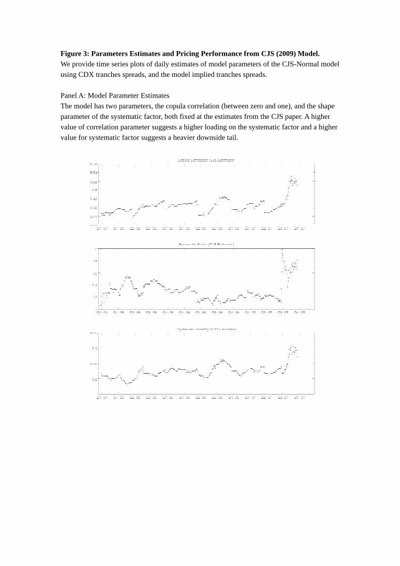
Figure 3: Parameters Estimates and Pricing Performance from CJS (2009) Model.

We provide time series plots of daily estimates of model parameters of the CJS-Normal model

using CDX tranches spreads, and the model implied tranches spreads.

Panel A: Model Parameter Estimates

The model has two parameters, the copula correlation (between zero and one), and the shape

parameter of the systematic factor, both fixed at the estimates from the CJS paper. A higher

value of correlation parameter suggests a higher loading on the systematic factor and a higher

value for systematic factor suggests a heavier downside tail.

Panel B: Pricing Performance

This figure plots the implied tranches spreads (up-front for the equity tranche) from the model

and the actual tranche spreads for all the standardized CDX tranches during our sample, as

well as the daily RMSE (pricing errors defined as (data-model)/model) of the five tranches.

Over the sample period, the average RMSE for five year CDX tranches is 1584.1%.

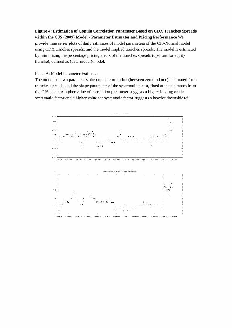
Figure 4: Estimation of Copula Correlation Parameter Based on CDX Tranches Spreads

within the CJS (2009) Model - Parameter Estimates and Pricing Performance We

provide time series plots of daily estimates of model parameters of the CJS-Normal model

using CDX tranches spreads, and the model implied tranches spreads. The model is estimated

by minimizing the percentage pricing errors of the tranches spreads (up-front for equity

tranche), defined as (data-model)/model.


The model has two parameters, the copula correlation (between zero and one), estimated from

tranches spreads, and the shape parameter of the systematic factor, fixed at the estimates from

the CJS paper. A higher value of correlation parameter suggests a higher loading on the

systematic factor and a higher value for systematic factor suggests a heavier downside tail.

Figure 5: Alternative Distribution Assumption for the Idiosyncratic Factor within the

the CJS (2009) Model - Parameter Estimates and Pricing Performance of the CJS-T(3)

Copula Model.

We change the distribution assumption for the idiosyncratic factor in the CJS model from

normal to student's t with degree of freedom 3, which has a heavy tail distribution. We

provide time series plots of daily estimates of model parameters of the CJS-T(3) model using

CDX tranches spreads, and the model implied tranches spreads. The model is estimated by

minimizing the percentage pricing errors of the tranches spreads (up-front for equity tranche),

defined as (data-model)/model.






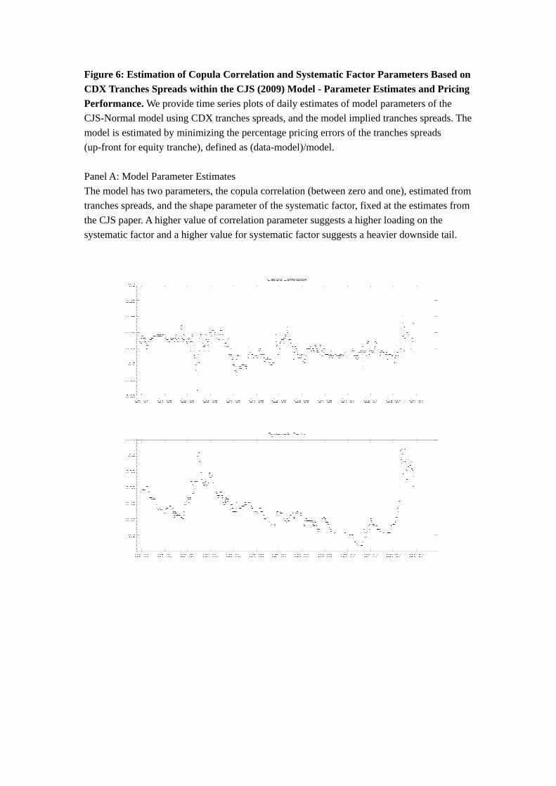
Figure 6: Estimation of Copula Correlation and Systematic Factor Parameters Based on

CDX Tranches Spreads within the CJS (2009) Model - Parameter Estimates and Pricing

Performance. We provide time series plots of daily estimates of model parameters of the

CJS-Normal model using CDX tranches spreads, and the model implied tranches spreads. The

model is estimated by minimizing the percentage pricing errors of the tranches spreads

(up-front for equity tranche), defined as (data-model)/model.






Figure 7: Parameter Estimates and Pricing Performance of the Double-t Copula Model

Based on CDX Tranches Spreads.

We change the distribution assumptions for the systematic and idiosyncratic factor in the CJS

model student's t distributions with the degree of freedom parameters estimated from the data.

We provide time series plots of daily estimates of model parameters of the Double-t model

using CDX tranches spreads, and the model implied tranches spreads. The model is estimated

by minimizing the percentage pricing errors of the tranches spreads (up-front for equity

tranche), defined as (data-model)/model.


The model has three parameters, the copula correlation (between zero and one) and the

inverse of the degrees of freedom of the systematic and idiosyncratic factors (between zero

and 0.5). A higher value of correlation parameter suggests a higher loading on the systematic

factor and a higher value for systematic/idiosyncratic factor suggests a heavier downside tail.

Figure 8: Joint Pricing of CDX Tranches Spreads and OTM Index Put Options -

Parameter Estimates and Pricing Performance of the Double-t Copula Model.

We change the distribution assumptions for the systematic and idiosyncratic factor in the CJS

model student's t distributions with the degree of freedom parameters estimated from the data.

We provide time series plots of daily estimates of model parameters of the Double-t model

using CDX tranches spreads and Index options prices, and the model implied tranches spreads

and options prices. The model is estimated by minimizing the percentage pricing errors of the

tranches spreads (up-front for equity tranche) and options prices, defined as

(data-model)/model.


The model has three parameters, the copula correlation (between zero and one) and the

inverse of the degrees of freedom of the systematic and idiosyncratic factors (between zero

and 0.5). A higher value of correlation parameter suggests a higher loading on the systematic

factor and a higher value for systematic/idiosyncratic factor suggests a heavier downside tail.

Panel B: Pricing Performance of CDX tranches





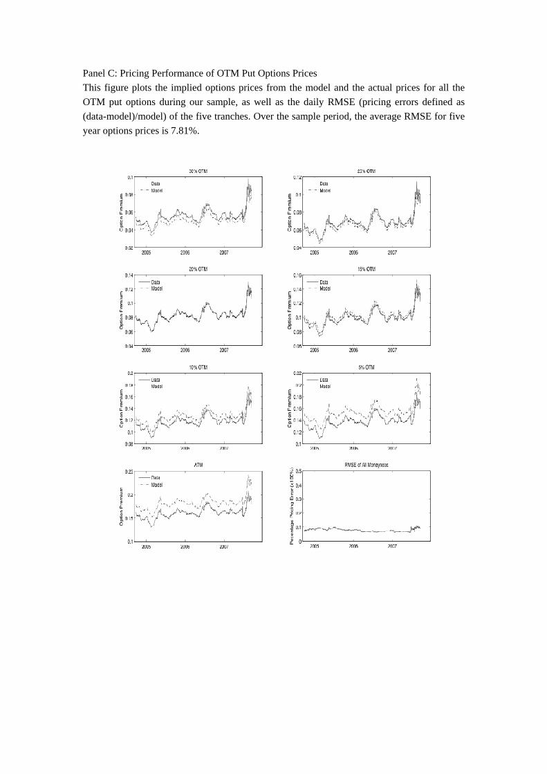
Panel C: Pricing Performance of OTM Put Options Prices

This figure plots the implied options prices from the model and the actual prices for all the

OTM put options during our sample, as well as the daily RMSE (pricing errors defined as

(data-model)/model) of the five tranches. Over the sample period, the average RMSE for five

year options prices is 7.81%.

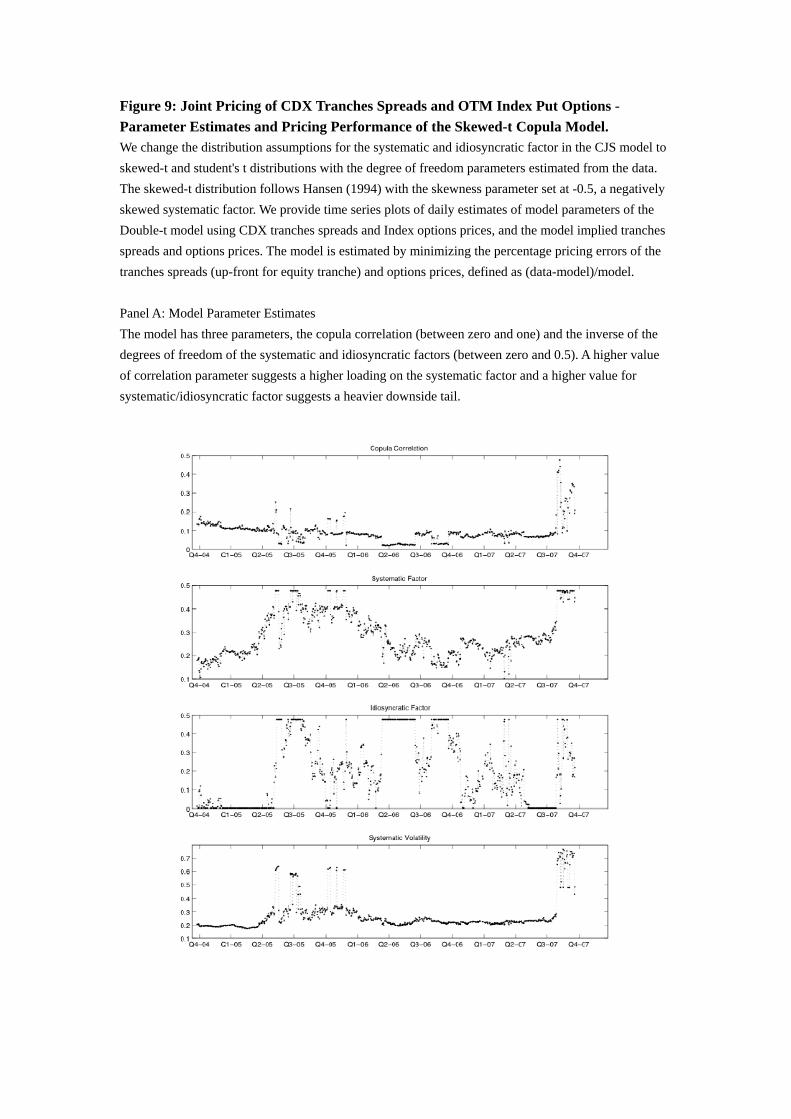
Figure 9: Joint Pricing of CDX Tranches Spreads and OTM Index Put Options -

Parameter Estimates and Pricing Performance of the Skewed-t Copula Model. We change the distribution assumptions for the systematic and idiosyncratic factor in the CJS model to

skewed-t and student's t distributions with the degree of freedom parameters estimated from the data.

The skewed-t distribution follows Hansen (1994) with the skewness parameter set at -0.5, a negatively

skewed systematic factor. We provide time series plots of daily estimates of model parameters of the

Double-t model using CDX tranches spreads and Index options prices, and the model implied tranches

spreads and options prices. The model is estimated by minimizing the percentage pricing errors of the

tranches spreads (up-front for equity tranche) and options prices, defined as (data-model)/model.


The model has three parameters, the copula correlation (between zero and one) and the inverse of the

degrees of freedom of the systematic and idiosyncratic factors (between zero and 0.5). A higher value

of correlation parameter suggests a higher loading on the systematic factor and a higher value for

systematic/idiosyncratic factor suggests a heavier downside tail.

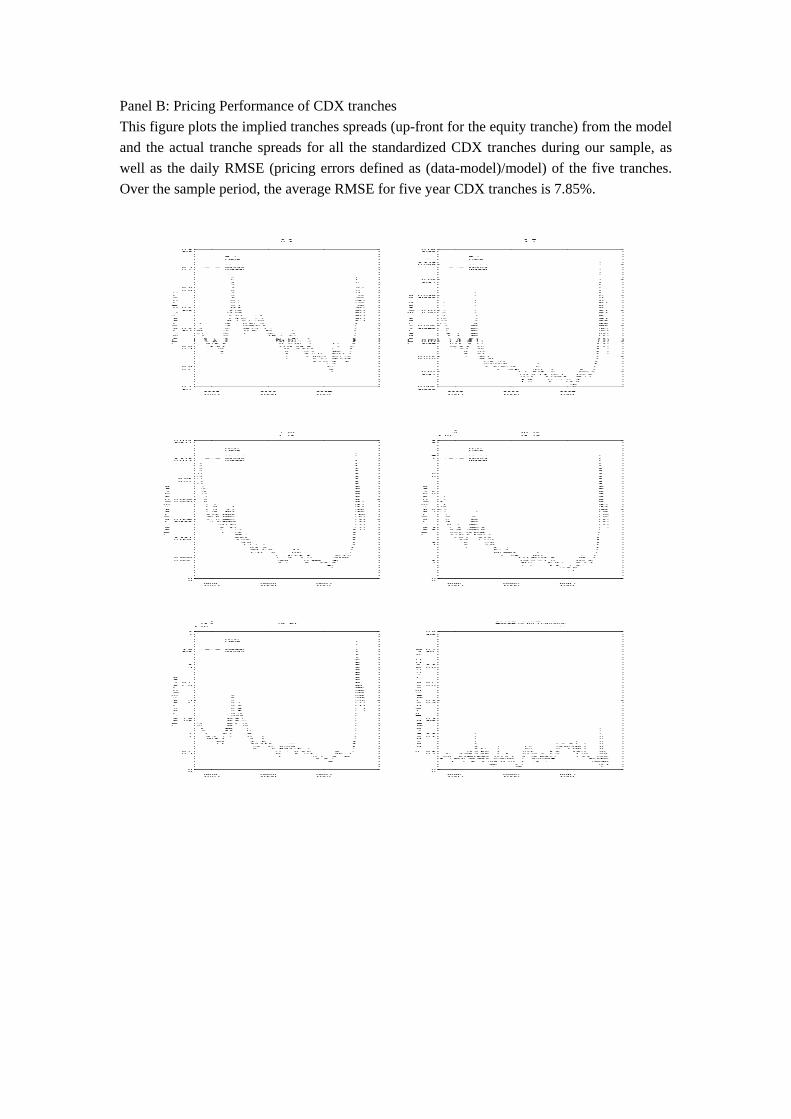
Panel B: Pricing Performance of CDX tranches





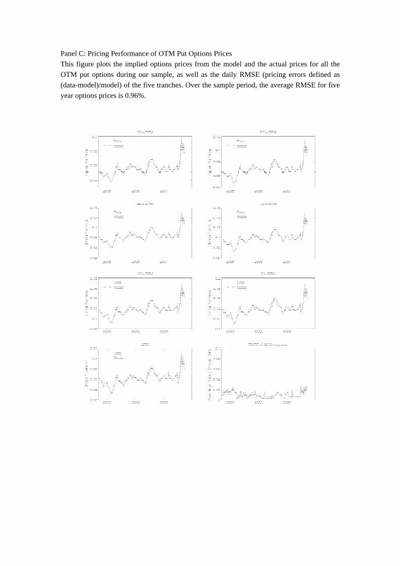
Panel C: Pricing Performance of OTM Put Options Prices

This figure plots the implied options prices from the model and the actual prices for all the

OTM put options during our sample, as well as the daily RMSE (pricing errors defined as

(data-model)/model) of the five tranches. Over the sample period, the average RMSE for five

year options prices is 0.96%.

Download - Economic Catastrophe Bonds: Ine cient Market or Inadequate ... Catastrophe... · Economic Catastrophe Bonds: Ine cient Market or Inadequate Model? ABSTRACT In an in uential paper,

Top Related