arX
iv:2
101.
1205
1v4
[cs
.IT
] 1
1 N
ov 2
021
1
Edge Federated Learning Via Unit-Modulus
Over-The-Air Computation
Shuai Wang, Yuncong Hong, Rui Wang, Qi Hao, Yik-Chung Wu, and Derrick Wing Kwan Ng
Abstract
Edge federated learning (FL) is an emerging paradigm that trains a global parametric model
from distributed datasets based on wireless communications. This paper proposes a unit-modulus over-
the-air computation (UMAirComp) framework to facilitate efficient edge federated learning, which
simultaneously uploads local model parameters and updates global model parameters via analog beam-
forming. The proposed framework avoids sophisticated baseband signal processing, leading to low
communication delays and implementation costs. Training loss bounds of UMAirComp FL systems
are derived and two low-complexity large-scale optimization algorithms, termed penalty alternating
minimization (PAM) and accelerated gradient projection (AGP), are proposed to minimize the nonconvex
nonsmooth loss bound. Simulation results show that the proposed UMAirComp framework with PAM
algorithm achieves a smaller mean square error of model parameters’ estimation, training loss, and
test error compared with other benchmark schemes. Moreover, the proposed UMAirComp framework
with AGP algorithm achieves satisfactory performance while reduces the computational complexity
by orders of magnitude compared with existing optimization algorithms. Finally, we demonstrate the
implementation of UMAirComp in a vehicle-to-everything autonomous driving simulation platform. It
is found that autonomous driving tasks are more sensitive to model parameter errors than other tasks
since the neural networks for autonomous driving contain sparser model parameters.
Index Terms
Analog beamforming, autonomous driving, federated learning, large-scale optimization.
Part of this paper has been presented at the IEEE Global Communications Conference (GLOBECOM), Madrid, Spain, Dec. 2021 [46].
Shuai Wang is with the Department of Electrical and Electronic Engineering, the Department of Computer Science and Engineering, and
the Sifakis Research Institute of Trustworthy Autonomous Systems, Southern University of Science and Technology (SUSTech), Shenzhen
518055, China (e-mail: [email protected]). Yuncong Hong and Rui Wang are with the Department of Electrical and Electronic
Engineering, Southern University of Science and Technology (SUSTech), Shenzhen 518055, China (e-mail: [email protected];
[email protected]). Qi Hao is with the Department of Computer Science and Engineering and the Sifakis Research Institute of Trustworthy
Autonomous Systems, Southern University of Science and Technology (SUSTech), Shenzhen 518055, China (e-mail: [email protected]).
Yik-Chung Wu is with the Department of Electrical and Electronic Engineering, The University of Hong Kong, Hong Kong (e-mail:
[email protected]). Derrick Wing Kwan Ng is with the School of Electrical Engineering and Telecommunications, the University of New
South Wales, Australia (email: [email protected]). Corresponding Author: Rui Wang and Qi Hao.
2
I. INTRODUCTION
Deep learning has achieved unprecedented breakthrough in image classification, speech recog-
nition, and object detection due to its ability to efficiently extract intricate nonlinear features from
high-dimensional data [1]. Typically, a cloud center collects data from distributed users and trains
a centralized model via gradient-based back propagation [2]–[5]. However, since the users need
to share their local data to the cloud, this paradigm could lead to some potential privacy issues,
hindering the development of deep learning in extensive applications such as smart cities and
financial systems.
To address the privacy issue, federated learning (FL), which trains individual deep learning
models at user terminals, has been proposed by Google Research [6]. In the framework of FL,
the locally generated data is locally adopted and not shared to any third party. To leverage the
knowledge from other users, local model parameters are uploaded periodically to a server for
model aggregation and the aggregated global parameters are broadcast to the users for further
local updates. Therefore, FL achieves distributed training while ensuring data privacy [7].
A. Edge Federated Learning and Related Work
FL was originally developed for wire-line connected systems [8]. To achieve ubiquitous
intelligence, a promising solution is edge FL, e.g., [7]–[17], where users are connected to an
edge server via wireless links. However, the convergence of edge FL may take a long time due
to limited capacity of wireless channels during the uplink model aggregation step. To reduce
the transmission delay, various edge FL designs have been proposed (summarized in Table I1),
which are mainly categorized into digital modulation [8]–[13] and analog modulation [14]–[17]
methods.
For digital modulation and single-antenna systems, data from different users are multiplexed
either in the time or the frequency domain. Current works on delay reduction focus on reducing
1) the number of model aggregation iterations [9], 2) the number of users [10], or 3) the number
of bits for representing the gradient of back propagation in each iteration [12]. However, since
these strategies involve approximation or simplification of the FL procedure, the performance of
learning would be degraded inevitably. Another way to reduce the transmission delay is to adopt
1For more related work on digital and analog federated learning, please refer to [7].
3
TABLE I: A Comparison of Existing and Proposed Schemes.
Modulation Work MIMORF
Chain
Alg.
Complex.
Commun.
Delay
Objective
FunctionAirComp
FL
Task
Digital
[8] % + + +++ N/A % Classification
[9], [10] % + + ++ Loss Bound % Classification
[12] % + + ++ Loss Bound % Classification
[13] Digital +++ +++ ++ MSE % %
Analog
[14], [15] % + + + Heuristic ! Classification
[16] Digital +++ +++ + MSE ! Classification
[17] Digital +++ ++ + Noise Variance ! Classification
Ours Analog + + + Loss Bound ! Object Detection
The symbol “+” means low, “++” means moderate, “+++” means high.
The symbol “X” means functionality supported, “%” means functionality not supported.
multiple-input multiple-output (MIMO) technology for transmission so that data from multiple
users are multiplexed concurrently in the spatial domain [13].
On the other hand, the key advantage of analog modulation [14]–[17] over digital modulation
arises from the ground-breaking idea of over-the-air computation (AirComp). Specifically, if mul-
tiple users upload their local parameters simultaneously, a superimposed signal, which represents
a weighted sum of individual model parameters, is observed at the edge server. By performing
minimum mean square error (MMSE) detection on the superimposed signal, an estimate of the
global parameter vector can be obtained. This significantly saves the transmission time since
AirComp in fact exploits inter-user interference in the simultaneous user transmission [18]–[20],
in oppose to interference suppression as in digital modulation. However, due to channel fading
and noise in wireless systems, AirComp employed in single-antenna systems [14], [15] could
result in a large error in the estimation of global model parameters at the edge server, leading to
slow convergence of FL. As a remedy, adopting MIMO beamforming [16], [17] could reduce the
parameter transmission error by aligning the beams carrying the local parameters’ information
to the same spatial direction. However, the current transmit and receive beamforming designs in
MIMO AirComp systems involve exceedingly high radio frequency (RF) chain costs and high
computational complexities [16], [17], preventing their practical implementation.
In practice, both digital and analog modulation methods share the same goal, i.e., minimizing
the training loss function. However, due to the lack of an explicit form of the training loss

4
function with respect to wireless designs, most works focus on other related objective functions
such as mean square error (MSE) [16] and noise variance [17]. Recently, the relationship between
the training loss function and the wireless designs is derived in [9]–[11], [21], [22]. Nonetheless,
the bounds in [9]–[11], [21], [22] are only applicable if the global model parameters are perfectly
broadcast to users. For practical cases involving errors in the model broadcast phase, new training
loss bounds are required to capture the training performance, which remains an open problem.
B. Summary of Challenges and Contributions
In summary, despite recent exciting development of edge FL techniques, e.g., [8]–[17], a
number of technical challenges remain to be overcome, including
1) Analog beamforming design under federated learning settings. Analog beamforming
with a proper phase shift network design [23], [24] can help reduce implementation costs
compared with digital beamfroming in [16], [17], which has not been studied in edge FL
systems, yet. Since the analog beamformer is unit-modulus, it introduces a large number
of intractable nonconvex and nonsmooth constraints. Furthermore, the analog beamformer
in FL systems aims to minimize the FL training loss bound, which is a non-differentiable
function of the beamforming design. This is different from the conventional analog beam-
forming designs in massive MIMO systems that aim to decode individual information from
each user [23], [24].
2) Reduction of beamforming design complexities. Most beamforming algorithms [13],
[16], [17], [24] rely on the execution of the interior point method (IPM). Yet, since IPM
involves the inversion of Hessian matrices, these algorithms are with high computational
complexities requiring exceedingly long signal processing delay, especially when massive
MIMO technique is applied. On the other hand, first-order methods [38]–[40] (i.e., no
inversion of Hessian matrices) could lead to significantly lower computational complexities
than that of the IPM. However, they cannot directly handle the analog beamforming design
problem due to the non-differentiable training loss bound and unit-modulus constraints.
3) Verification of robustness in more complex learning tasks. Existing algorithms in [8]–
[17] are mainly tested on simple image classification tasks (e.g., recognition of handwritten
digits). Experiments on more complex and closer-to-reality tasks, such as 3D object detection
[25], [26] in vehicle-to-everything (V2X) autonomous driving systems, are needed to verify
the robustness of edge FL. However, the associated implementation involves scenario gener-
5
ation, multi-modal data generation, multi-sensor calibration, multi-vehicle synchronization
and coordinate transformation, label generation, and object detection.
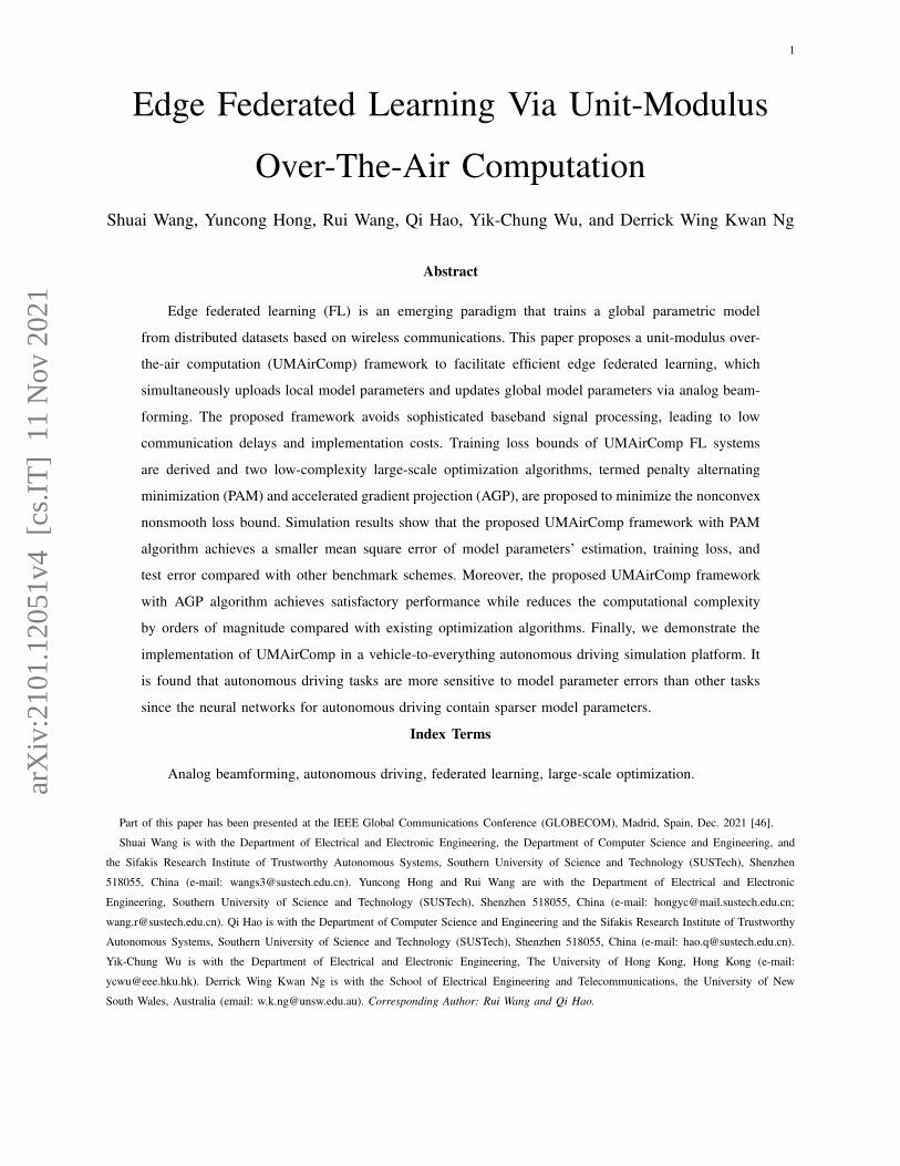
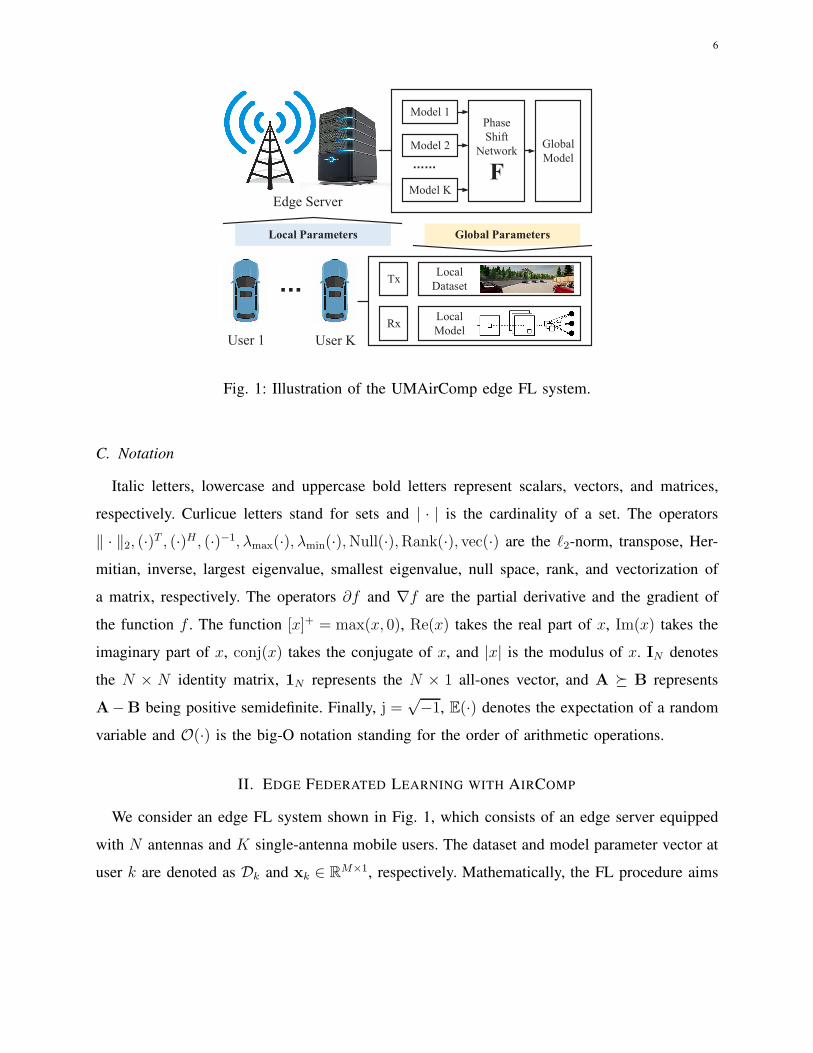
To fill the research gap, this paper proposes the unit-modulus AirComp (UMAirComp) frame-
work for edge FL in MIMO communication systems, as shown in Fig. 1. The UMAirComp
framework consists of multiple edge users with local sensing data (e.g., autonomous driving
cars generate camera images and light detection and ranging (LiDAR) point clouds of the
environment), an edge server for performing model aggregation, and communication interfaces
for exchanging model parameters. Specifically, the edge users update their local models using
the local training datasets separately. Then, the trained model parameters are transformed into
signals via analog modulation and uploaded to the server. To reduce the implementation cost of
RF chains, the edge server does not process the received signals at the baseband. Instead, it applies
a phase shift network (either a fully-connected structure or a partially-connected structure) in the
RF domain for global model aggregation and broadcasting. All users decode model parameters
from the received broadcast signals via analog demodulation. The advantages of UMAirComp
and contributions of this paper are summarized below:
1) The UMAirComp at the server significantly reduces the required implementation cost of RF
chains in MIMO FL systems, thereby reducing the hardware and energy costs. To understand
how UMAirComp works, the training loss of UMAirComp framework is proved to be upper
bounded by a monotonic increasing function of the maximum MSE of the model parameters’
estimation.
2) Despite the UMAirComp problem being highly nonconvex, two large-scale optimization
algorithms, termed penalty alternating minimization (PAM) and accelerated gradient pro-
jection (AGP), are developed for fully-connected UMAirComp and partially-connected
UMAirComp, respectively. The learning performance of the proposed PAM and AGP is
shown to outperform other benchmark schemes. In particular, the AGP algorithm is 100x
faster than that of the state-of-the-art optimization algorithms.
3) We implement the UMAirComp edge FL scheme for 3D object detection with multi-vehicle
point-cloud datasets in CARLA simulation platform [27]. To the best of our knowledge,
this is the first attempt that edge FL is demonstrated in a V2X auto-driving simulator with
a close-to-reality task.
6
Edge Server
User 1
Tx
User K
Phase
Shift
Network
F
Model 2
Model K
Model 1
Global
Model
Rx
Local Parameters Global Parameters
Local
Dataset
Local
Model
Fig. 1: Illustration of the UMAirComp edge FL system.
C. Notation
Italic letters, lowercase and uppercase bold letters represent scalars, vectors, and matrices,
respectively. Curlicue letters stand for sets and | · | is the cardinality of a set. The operators
‖ · ‖2, (·)T , (·)H, (·)−1, λmax(·), λmin(·),Null(·),Rank(·), vec(·) are the ℓ2-norm, transpose, Her-
mitian, inverse, largest eigenvalue, smallest eigenvalue, null space, rank, and vectorization of
a matrix, respectively. The operators ∂f and ∇f are the partial derivative and the gradient of
the function f . The function [x]+ = max(x, 0), Re(x) takes the real part of x, Im(x) takes the
imaginary part of x, conj(x) takes the conjugate of x, and |x| is the modulus of x. IN denotes
the N × N identity matrix, 1N represents the N × 1 all-ones vector, and A � B represents
A−B being positive semidefinite. Finally, j =√−1, E(·) denotes the expectation of a random
variable and O(·) is the big-O notation standing for the order of arithmetic operations.
II. EDGE FEDERATED LEARNING WITH AIRCOMP
We consider an edge FL system shown in Fig. 1, which consists of an edge server equipped
with N antennas and K single-antenna mobile users. The dataset and model parameter vector at
user k are denoted as Dk and xk ∈ RM×1, respectively. Mathematically, the FL procedure aims

7
to solve the following optimization problem:
min{xk},θ
1∑K
k=1 |Dk|
K∑
k=1
∑
dk,l∈Dk
Θ(dk,l, θ)
︸ ︷︷ ︸:=Λ(θ)
s.t. x1 = · · · = xK = θ, (1)
where Θ(dk,l, θ) is the loss function corresponding to a single sample dk,l (1 ≤ l ≤ |Dk|) in Dk
given parameter vector θ, while Λ(θ) denotes the global loss function to be minimized.
The objective function can be rewritten into a separable form Λ(θ) =∑K
k=1 αkλk(xk), where
λk(xk) = 1|Dk|
∑dk,l∈Dk
Θ(dk,l,xk) is the loss function at the k-th user and αk = |Dk|∑Kl=1 |Dl|
.
Therefore, the training of FL model parameters (i.e., solving (1)) in the considered edge system
is naturally a distributed and iterative procedure, where each iteration involves four steps:
1) updating the local parameter vectors (x1, · · · ,xK) for minimizing (λ1, · · · , λK) with re-
spect to {D1, · · · ,DK} at users (1, · · · , K), respectively; 2) transforming the local parameters
(x1, · · · ,xK) into symbols (s1, · · · , sK) for uploading; 3) aggregating (s1, · · · , sK) in an analog
manner at the edge server and broadcasting the results to the users. 4) receiving the signals
(y1, · · · ,yK) at the users and transforming (y1, · · · ,yK) into parameters (x1, · · · ,xK) for next-
round updates. The above four steps are elaborated below.
1) Step 1: Let x[i]k (0) ∈ RM×1 be the local parameter vector at user k at the beginning of
the i-th iteration (i ≥ 0 and x[0]k (0) = θ[0]). To update x
[i]k (0), user k minimizes the loss
function λk(xk) via gradient descent2 as
x[i]k (τ + 1) = x
[i]k (τ)−
ε
|Dk|∑
dk,l∈Dk
∇xΘ (dk,l,x)∣∣x=x
[i]k(τ), k = 1, · · · , K, (2)
where ε is the step-size and τ is from 0 to E−1 with E being the number of local updates.
2) Step 2: All users upload {x[i]k (E)|∀k} to the edge server. Specifically, user k modulates its
local parameter vector x[i]k (E) into a complex vector s
[i]k ∈ CS×1 in an analog manner as in
[14], [15], where
s[i]k =
√p[i]k exp(jϕ
[i]k )√
2η[i]
[x[i]k,1(E) + j x
[i]k,2(E), · · · , x[i]
k,M−1(E) + j x[i]k,M(E)
]T. (3)
In (3), S = M/2 is the vector dimension and x[i]k,m(E) is the m-th element of x
[i]k (E).
The scaling factor η[i] is η[i] = 1K
∑Kk=1
1M‖x[i]
k (E)‖22 such that the average power of s[i]k
2If |Dk| is large, stochastic gradient descent can be adopted to accelerate the training speed.

8
is 1SE
[‖s[i]k ‖22
]= p
[i]k .3 The transmit power is p
[i]k ≤ P0 with P0 being the maximum
transmit power at each user and the phase shift is ϕ[i]k ∈ [0, 2π]. To facilitate the subsequent
derivations, we define the transmitter design t[i]k =
√p[i]k exp(jϕ
[i]k ) for all (i, k) and {p[i]k , ϕ
[i]k }
can be recovered from {t[i]k }.3) Step 3: The received signal R[i] ∈ CN×S at the server is
R[i] =K∑
k=1
h[i]k (s
[i]k )
T + Z[i], (4)
where h[i]k ∈ C
N×1 is the uplink channel vector from user k to the server and Z[i] ∈ CN×S is
the matrix of the additive white Gaussian noise with covariance matrix E[vec(Z[i])vec(Z[i])H
]=
σ2b INS (σ2
b is the noise power at the server). Upon receiving the superimposed signal, the
server processes R[i] using a function Ψ[i](·) and broadcasts Ψ[i](R[i]) ∈ CN×S to all the
users.
4) Step 4: The received signal at user k is
(y[i]k
)T=(g[i]k
)HΨ[i]
(R[i])+(n[i]k
)T, (5)
where g[i]k ∈ CN×1 is the downlink channel vector4 from the server to user k and n
[i]k ∈ CS×1
is the vector of the additive white Gaussian noise with covariance matrix σ2kIS (σ2
k is the
noise power at user k). User k applies demodulates y[i]k and sets the local parameter vector
for the (i+ 1)-th iteration as
x[i+1]k (0) =
√2η[i]
[Re(r
[i]k y
[i]k,1), Im(r
[i]k y
[i]k,1), · · · ,Re(r
[i]k y
[i]k,L), Im(r
[i]k y
[i]k,L)]T
, (6)
where r[i]k ∈ C is a receive coefficient applied to y
[i]k and y
[i]k,l is the lth element of y
[i]k . This
completes one federated learning round and we set i← i+ 1.
The entire procedure stops when i = R with R being the number of federated learning rounds.
III. PROPOSED UMAIRCOMP EDGE FL FRAMEWORK
In existing AirComp schemes, e.g., [14]–[17], Ψ[i] is implemented using baseband signal
processing techniques. Thus, the superimposed signals of all receive antennas at the edge server
are first combined via a vector in the digital baseband and then broadcast to users via another
3In practice, the users would adopt η[i−1] sent from the server in the last iteration, which is a good approximation for the
actual η[i] in the current iteration.
4It is assumed that {h[i]k ,g
[i]k } are quasi-static flat-fading channels during the model exchange procedure of each FL iteration.
9
vector in the baseband. Therefore, the associated implementation cost could be high if massive
number of antennas are deployed. In the following, the UMAirComp scheme, where the functions
{Ψ[i]} are implemented in analog domain, is proposed. This helps to reduce both the required
implementation costs and power consumptions while achieving excellent system performance.
A. UMAirComp Framework
The proposed UMAirComp scheme employs multiple phase shifters to generate the updated
global model parameters from the local ones. Specifically, we propose to aggregate and forward
the signal via
Ψ[i](R[i]) =√γ F[i]R[i], (7)
where γ > 0 is the power scaling factor at the edge server and F[i] ∈ CN×N is the phase
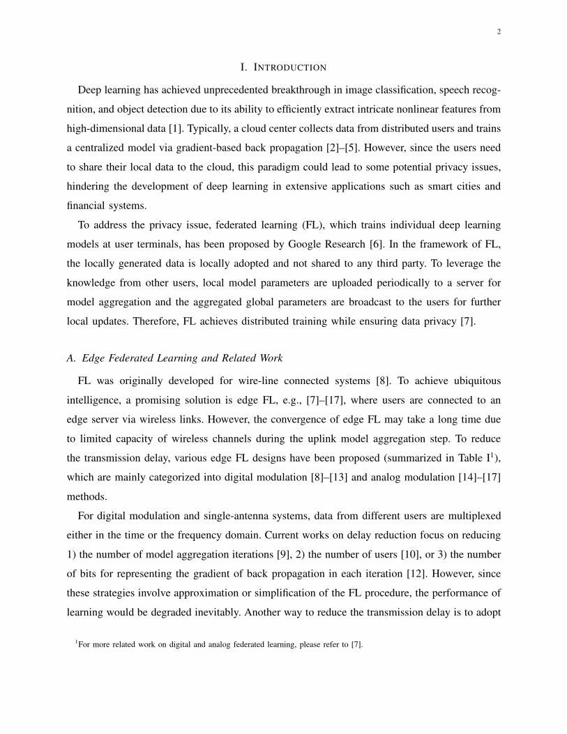
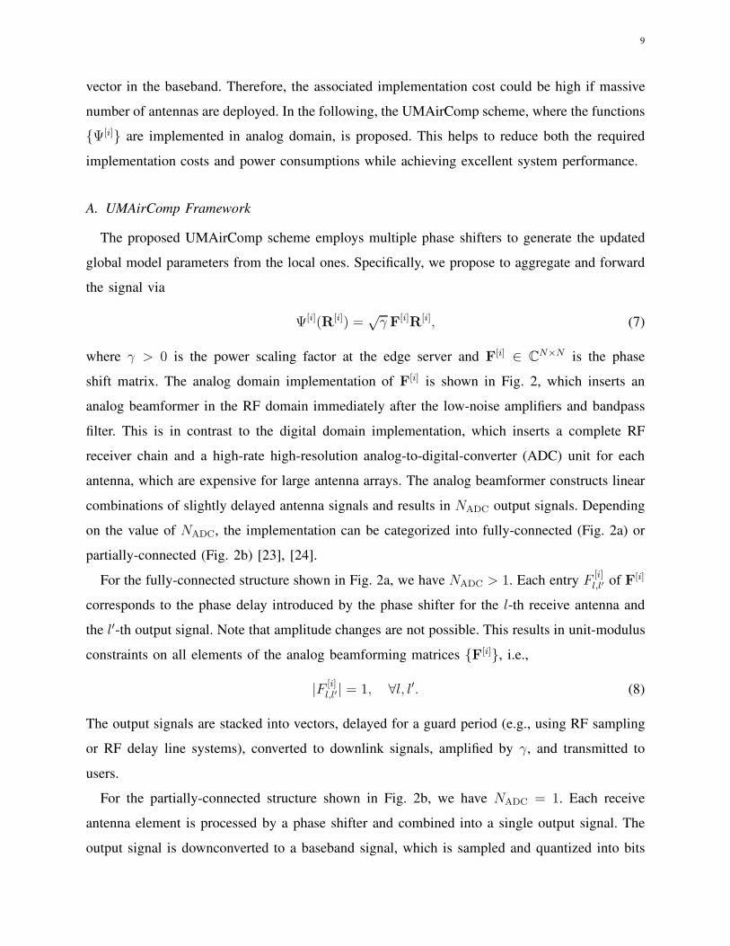
shift matrix. The analog domain implementation of F[i] is shown in Fig. 2, which inserts an
analog beamformer in the RF domain immediately after the low-noise amplifiers and bandpass
filter. This is in contrast to the digital domain implementation, which inserts a complete RF
receiver chain and a high-rate high-resolution analog-to-digital-converter (ADC) unit for each
antenna, which are expensive for large antenna arrays. The analog beamformer constructs linear
combinations of slightly delayed antenna signals and results in NADC output signals. Depending
on the value of NADC, the implementation can be categorized into fully-connected (Fig. 2a) or
partially-connected (Fig. 2b) [23], [24].
For the fully-connected structure shown in Fig. 2a, we have NADC > 1. Each entry F[i]l,l′ of F[i]
corresponds to the phase delay introduced by the phase shifter for the l-th receive antenna and
the l′-th output signal. Note that amplitude changes are not possible. This results in unit-modulus
constraints on all elements of the analog beamforming matrices {F[i]}, i.e.,
|F [i]l,l′| = 1, ∀l, l′. (8)
The output signals are stacked into vectors, delayed for a guard period (e.g., using RF sampling
or RF delay line systems), converted to downlink signals, amplified by γ, and transmitted to
users.
For the partially-connected structure shown in Fig. 2b, we have NADC = 1. Each receive
antenna element is processed by a phase shifter and combined into a single output signal. The
output signal is downconverted to a baseband signal, which is sampled and quantized into bits
10
+
+
UL
-DL
Guard
Perio
d
Do
wn
link
Tran
smissio
n
Low Noise
AmplifierPhase
ShifterCombinerSplitter
High Power
Amplifier
F1,1
FN,1
F1,1
(a)
+ RF-BB ADC
UL
-DL
Gu
ard P
eriod
Do
wn
link
Tran
smissio
nHigh Power
Amplifier
Low Noise
Amplifier
Phase
Shifter
Combiner
Splitter
(b)
Fig. 2: Illustration of the phase shift network at the server: a) fully-connected structure; b)
partially-connected strucutre.
via an ADC unit. After delaying for a guard period, the signal is upconverted to a passband
signal and filtered via another phase shift vector before transmission. Hence, apart from the unit-
modulus constraint (8), F[i] should also satisfy Rank(F[i])= 1. Note that the required number
of total phase shifters is only 2N for the partially-connected structure.
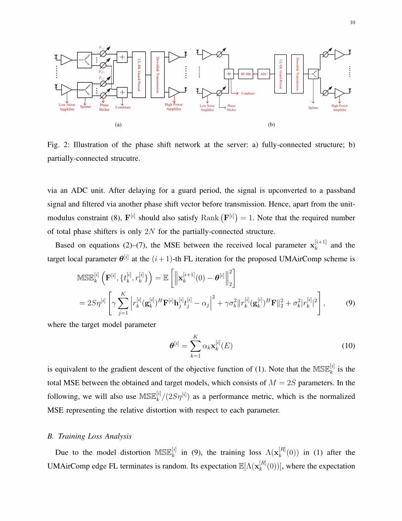
Based on equations (2)–(7), the MSE between the received local parameter x[i+1]k and the
target local parameter θ[i] at the (i+1)-th FL iteration for the proposed UMAirComp scheme is
MSE[i]k
(F[i], {t[i]k , r
[i]k })= E
[∥∥∥x[i+1]k (0)− θ[i]
∥∥∥2
2
]
= 2Sη[i]
[γ
K∑
j=1
∣∣∣r[i]k (g[i]k )
HF[i]h[i]j t
[i]j − αj
∣∣∣2
+ γσ2b‖r[i]k (g
[i]k )
HF‖22 + σ2k|r[i]k |2
], (9)
where the target model parameter
θ[i] =K∑
k=1
αkx[i]k (E) (10)
is equivalent to the gradient descent of the objective function of (1). Note that the MSE[i]k is the
total MSE between the obtained and target models, which consists of M = 2S parameters. In the
following, we will also use MSE[i]k /(2Sη
[i]) as a performance metric, which is the normalized
MSE representing the relative distortion with respect to each parameter.
B. Training Loss Analysis
Due to the model distortion MSE[i]k in (9), the training loss Λ(x
[R]k (0)) in (1) after the
UMAirComp edge FL terminates is random. Its expectation E[Λ(x[R]k (0))], where the expectation
11
is taken over channel noises and model parameters, would be greater than Λ(θ∗) in wired FL
systems, where θ∗ denotes the optimal solution of θ to (1). Hence, we can use their difference,
namely E[Λ(x[R]k (0))] − Λ(θ∗), as a metric to capture the degradation on training loss. Before
establishing the main results, we first introduce the assumption imposed on the loss function.
Assumption 1. (i) The function Λ(x) is µ-strongly convex. (ii) The function 1|Dk|
∑dk,l∈Dk
Θ(dk,l,x)
is twice differentiable and satisfies 1|Dk|
∑dk,l∈Dk
∇2xΘ(dk,l,x) � LI.
Under Assumption 1, the relationship between Λ(x[R]k (0)) and Λ(θ∗) is summarized in the
following theorem.
Theorem 1. With E = 1 and ε = 1L
, the UMAirComp scheme satisfies
E
[Λ(x
[R]k (0))
]− Λ(θ∗) ≤
R−1∑
i=0
A[i] maxk=1,··· ,K
MSE[i]k , (11)
as R→ +∞, where A[i] = L2
(3 + 2
∑Kj=1 α
2j
) (1− µ
L
)R−1−i.
Proof. Please refer to Appendix A.
Theorem 1 shows a diminishing A[i] → 0 for a large R − 1 − i, meaning that the impact
from earlier FL iterations vanishes as the edge FL continues. On the other hand, if MSE[i]k → 0
for all k, then Λ(x[R]k ) is an unbiased estimate of Λ(θ∗). This demonstrates the effectiveness of
UMAirComp in the asymptotic region. The convexity and smoothness in Assumption 1 have
been adopted in most loss bound analysis of FL (e.g., [21], [22], [28], [40]). Although it seems
to be restrictive for realistic applications, analysis under Assumption 1 could provide important
insights of the behavior of UMAirComp in nonconvex cases.
The analysis can be generalized to the case with multiple local epochs (i.e., E > 1). Specifi-
cally, in addition to Assumption 1, we further impose the following assumption.
Assumption 2. The gradient ‖ 1|Dk|
∑dk,l∈Dk
∇xΘ(dk,l,x)‖22 ≤ G2 for some G > 0 and all k.
In practice, the above assumption can always be satisfied with a sufficiently large G, which
represents the maximum gradient norm in the back propagation procedure. Otherwise, the explod-
ing gradients will lead to the unstable training of deep networks. Let Λ∗ denotes the minimum
training loss in (1) over all users’ datasets and λ∗k denotes the minimum training loss over
the k-th user’s dataset. Then, the degree of heterogeneity of the edge FL system is defined as

12
Γ = Λ∗ −∑Kk=1 αkλ
∗k. It can be seen that Γ = 0 if all users have the same dataset. Then the
following convergence result can be established.
Theorem 2. With ε = 2µ(ν+iE+τ)
and ν = max(8Lµ, E), the UM-AirComp scheme satisfies
E
[Λ(x
[R]k (0))
]− Λ(θ∗) ≤ 2Lmax(4C, µ2ν‖θ[0] − θ∗‖22)
µ2(RE + ν), (E1)
where
C = 8E2G2 + 6LΓ +µ2(ν +RE)2
4max∀i,k
MSE[i]k . (E2)
Proof. Please refer to Appendix B.
It can be seen from Theorem 2 that if we increase the number of local epochs E or the degree
of heterogeneity Γ, the term C would increase and the gap between E
[Λ(x
[R]k (0))
]and Λ(θ∗)
becomes larger. This implies that more local training epochs or more diverse datasets would
make it more difficult for the proposed UM-AirComp federated learning to converge.
C. Problem Formulation
Ideally, the optimization of {F[i], r[i]k , t
[i]k } should be performed to minimize the expectation
of training error, i.e., E[Λ(x[R]k (0))]. However, the analytical expression of E[Λ(x
[i+1]k (0))] is
usually challenging to derive. As a compromise, we resort to the minimization of the up-
per bound obtained from Theorem 1 or Theorem 2, which at least guarantees the worst-case
training loss performance. Minimizing the training loss bound is equivalent to minimizing∑R
i=0A[i]maxkMSE
[i]k for the case of E = 1 and max∀i,k MSE
[i]k for the case of E > 1. But
no matter E = 1 or E > 1, the objective function can be decoupled for each iteration and the
minimization at the i-th FL iteration, ∀i, is given by
P : minF, {rk,tk}
maxk=1,··· ,K
[γ
K∑
j=1
∣∣∣rkgHk Fhjtj − αj
∣∣∣2
+ γσ2b‖rk(gk)
HF‖22 + σ2k|rk|2
]
︸ ︷︷ ︸MSEk/(2ηS)
(12a)
s.t. F ∈ F , (12b)
|tk|2 ≤ P0, k = 1, · · · , K, (12c)
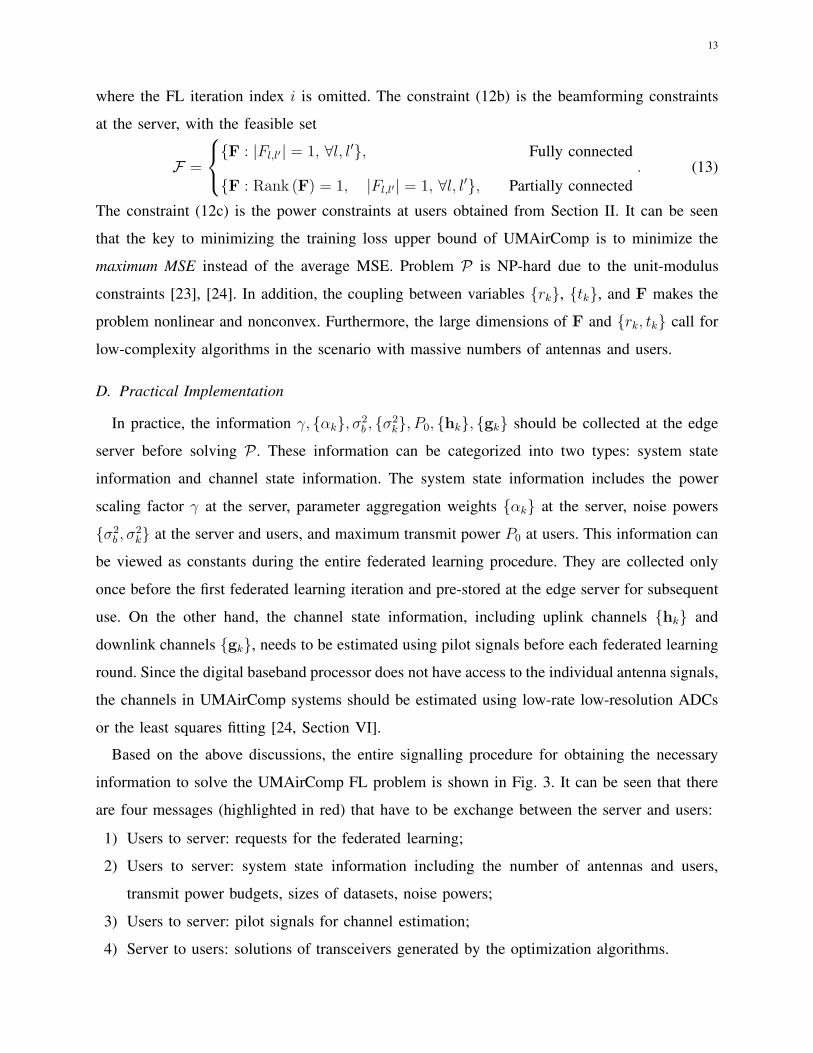
13
where the FL iteration index i is omitted. The constraint (12b) is the beamforming constraints
at the server, with the feasible set
F =
{F : |Fl,l′| = 1, ∀l, l′}, Fully connected
{F : Rank (F) = 1, |Fl,l′| = 1, ∀l, l′}, Partially connected
. (13)
The constraint (12c) is the power constraints at users obtained from Section II. It can be seen
that the key to minimizing the training loss upper bound of UMAirComp is to minimize the
maximum MSE instead of the average MSE. Problem P is NP-hard due to the unit-modulus
constraints [23], [24]. In addition, the coupling between variables {rk}, {tk}, and F makes the
problem nonlinear and nonconvex. Furthermore, the large dimensions of F and {rk, tk} call for
low-complexity algorithms in the scenario with massive numbers of antennas and users.
D. Practical Implementation
In practice, the information γ, {αk}, σ2b , {σ2
k}, P0, {hk}, {gk} should be collected at the edge
server before solving P . These information can be categorized into two types: system state
information and channel state information. The system state information includes the power
scaling factor γ at the server, parameter aggregation weights {αk} at the server, noise powers
{σ2b , σ
2k} at the server and users, and maximum transmit power P0 at users. This information can
be viewed as constants during the entire federated learning procedure. They are collected only
once before the first federated learning iteration and pre-stored at the edge server for subsequent
use. On the other hand, the channel state information, including uplink channels {hk} and
downlink channels {gk}, needs to be estimated using pilot signals before each federated learning
round. Since the digital baseband processor does not have access to the individual antenna signals,
the channels in UMAirComp systems should be estimated using low-rate low-resolution ADCs
or the least squares fitting [24, Section VI].
Based on the above discussions, the entire signalling procedure for obtaining the necessary
information to solve the UMAirComp FL problem is shown in Fig. 3. It can be seen that there
are four messages (highlighted in red) that have to be exchange between the server and users:
1) Users to server: requests for the federated learning;
2) Users to server: system state information including the number of antennas and users,
transmit power budgets, sizes of datasets, noise powers;
3) Users to server: pilot signals for channel estimation;
4) Server to users: solutions of transceivers generated by the optimization algorithms.
14
Send
requests
for
federated
learning
Establish
connections
& collect
system state
information
Channel
estimation
via direct
or indirect
method
(1)
Users
(2)
Server
(3)
Users
Update
local
models
with local
datasets
Aggregate
local models
via optimized
phase shifts
Local model
uploading
via optimized
transmitters
Global model
decoding
via optimized
receiversNo
Yes
Federated
Model
Execute
PAM or AGP
algorithms to
minimize the
loss bound
Broadcast
results of
transceiver
designs to
all users
(4)
Server
(5)
Server
(6)
Server
(7)
Users
(8)
Server
(9)
Users
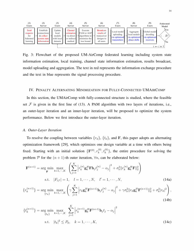
Fig. 3: Flowchart of the proposed UM-AirComp federated learning including system state
information estimation, local training, channel state information estimation, results broadcast,
model uploading and aggregation. The text in red represents the information exchange procedure
and the text in blue represents the signal processing procedure.
IV. PENALTY ALTERNATING MINIMIZATION FOR FULLY-CONNECTED UMAIRCOMP
In this section, the UMAirComp with fully-connected structure is studied, where the feasible
set F is given in the first line of (13). A PAM algorithm with two layers of iterations, i.e.,
an outer-layer iteration and an inner-layer iteration, will be proposed to optimize the system
performance. Below we first introduce the outer-layer iteration.
A. Outer-Layer Iteration
To resolve the coupling between variables {rk}, {tk}, and F, this paper adopts an alternating
optimization framework [29], which optimizes one design variable at a time with others being
fixed. Starting with an initial solution {F(0), r(0)k , t
(0)k }, the entire procedure for solving the
problem P for the (n+ 1)-th outer iteration, ∀n, can be elaborated below:
F(n+1) = arg minF
maxk=1,··· ,K
(K∑
j=1
∣∣∣r(n)k gHk Fhjt
(n)j − αj
∣∣∣2
+ σ2b‖r(n)k gH
k F‖22
)
s.t. |Fl,l′| = 1, l = 1, · · · , N, l′ = 1, · · · , N, (14a)
{r(n+1)k } = arg min
{rk}max
k=1,··· ,K
(γ
K∑
j=1
∣∣∣rkgHk F
(n+1)hjt(n)j − αj
∣∣∣2
+ γσ2b‖rkgH
k F(n+1)‖22 + σ2
k|rk|2),
(14b)
{t(n+1)k } = arg min
{tk}max
k=1,··· ,K
K∑
j=1
∣∣∣r(n+1)k gH
k F(n+1)hjtj − αj
∣∣∣2
s.t. |tk|2 ≤ P0, k = 1, · · · , K, (14c)

15
where {F(n), t(n)k , r
(n)k } is the solution at the n-th outer iteration. The iterative procedure stops
until n reaches the maximum iteration number n = Nmax.
Problem (14a) can be transferred to a convex problem via semidefinite relaxation (SDR) while
problems (14b) and (14c) are convex. Hence, problems (14a)–(14c) can all be solved via CVX
[32], a Matlab software package for solving convex problems based on interior point method
(IPM). According to [32], the computational complexity is at least O (N7) for solving (14a)
(the vectorization of F involves N2 variables) and O (K3.5) for solving (14b)–(14c). For large
N and K, this method is not desirable. In the following, a new algorithm termed PAM, which
decomposes (14a)–(14c) into smaller subproblems that are either solved by gradient updates
or closed-form updates, is proposed for achieving both excellent performance and significantly
lower computational complexities.
B. Inner-Layer Iteration
1) Optimization of F: Since F is a matrix, its vectorization is given as f = vec (F) ∈ CN2×1.
Applying Tr(AXBXT
)= vec(X)T
(BT ⊗A
)vec(X) [30], we have
r(n)k gH
k Fhjt(n)j = r
(n)k t
(n)j
(hTj ⊗ gH
k
)vec (F) = (a
(n)k,j )
Hf , (15)
σ2b‖r(n)k gH
k F‖22 = |r(n)k |2Tr(gkg
Hk FINF
H)= fHG
(n)k f , (16)
where G(n)k = σ2
b |r(n)k |2IN ⊗(gkg
Hk
)and a
(n)k,j =
[r(n)k t
(n)j
(hTj ⊗ gH
k
)]H. Problem (14a) is thus
re-formulated as
PF : minf
maxk=1,··· ,K
(K∑
j=1
∣∣∣(a(n)k,j )
Hf − αj
∣∣∣2
+ fHG(n)k f
)
s.t. |fl| = 1, l = 1, · · · , N2. (17)
To handle the nonseparable objective function, variable splitting of f is proposed such that
f = u1 = · · · = uK , where {uk} are auxilliary variables. Moreover, to handle the unit-modulus
constraints, another auxilliary variable z = f is introduced. For all the newly introduced equality
constraints, they can be transformed into quadratic penalties in the objective function [31]. As
a result, PF is approximately transformed into
minf ,z,{uk}
maxk=1,··· ,K
(K∑
j=1
∣∣∣(a(n)k,j )
Huk − αj
∣∣∣2
+ uHk G
(n)k uk
)+ ρ
(1
K
K∑
j=1
‖uj − f‖22 + ‖z− f‖22
)
s.t. |zl| = 1, l = 1, · · · , N2, (18)
16
where ρ is a tuning parameter. It can be proved that PF and (18) are equivalent problems as
ρ → +∞ [31]. However, this case also leads to the gradient norm of the objective function
of (18) being infinite, making (18) difficult to solve. Therefore, ρ controls the tradeoff between
approximation error and difficulty in solving (18).
We address (18) using alternating minimization, in which the cost function is iteratively
minimized with respect to one variable whereas the others are fixed. Starting with an initial
f (0) = z(0) = u(0)k,j = vec
(F(n)
), the whole process consists of iteratively solving
u(m+1)k = arg min
uk
K∑
j=1
∣∣∣(a(n)k,j )
Huk − αj
∣∣∣2
+ uHk G
(n)k uk +
ρ
K‖uk − f (m)‖22, ∀k, (19a)
f (m+1) = arg minf
ρ
(1
K
K∑
j=1
‖u(m+1)j − f‖22 + ‖z(m) − f‖22
), (19b)
z(m+1) = arg min|zl|=1,∀l
ρ‖z− f (m+1)‖22, (19c)
where m is the inner iteration index. It can be verified that the objective function of (18)
is strongly convex. Therefore, despite the non-differentiability of the objective, the alternating
minimization (19a)–(19c) is guaranteed to converge to a stationary point of (18) [29]. The iterative
procedure stops until m reaches the maximum iteration number m = Mmax.
The remaining question is how to solve (19a)–(19c) optimally. We notice that problems (19a)
and (19b) are standard least squares problems, thus their solutions are given by the following
closed-form expressions
u(m+1)k =
(K∑
j=1
a(n)k,j (a
(n)k,j )
H +G(n)k + ρI
)−1( K∑
j=1
αja(n)k,j +
ρ
Kf (m)
), (20)
f (m+1) =1
2
(1
K
K∑
j=1
u(m+1)j + z(m)
), (21)
respectively. On the other hand, problem (19c) is the projection of f (m+1) onto unit-modulus
constraint and the optimal solution is simply
z(m+1) = exp(j∠f (m+1)
). (22)
2) Optimization of {rk}: The problem of optimizing {rk} in (14b) is also a least squares
problem. The optimal solution is found by setting the derivative ∂MSEk/∂conj(rk) to zero:
∂MSEk
∂conj(rk)= γ
K∑
j=1
(rkg
Hk F
(n+1)hjt(n)j − αj
)conj
(gHk F
(n+1)hjt(n)j
)
17
+ γσ2b‖gH
k F(n+1)‖22rk + σ2
krk = 0 (23)
which yields
r(n+1)k =
∑Kj=1 αjconj
(gHk F
(n+1)hjt(n)j
)
∑Kj=1 |gH
k F(n+1)hjt
(n)j |2 + σ2
b‖gHk F
(n+1)‖22 + σ2k/γ
. (24)
3) Optimization of {tk}: The objective function of problem (14c) is not separable. Following
similar variable splitting procedure as in (18), we introduce auxiliary variables {ξk,j = tk, ∀k, j}and add quadratic penalty ρ
∑Kk=1
∑Kj=1 |ξk,j− tk|2 to the objective function. The problem (14c)
is approximately transformed into
Pt : min{tk ,ξk,j}
ρK∑
k=1
K∑
j=1
|ξk,j − tj|2 + maxk=1,··· ,K
K∑
j=1
∣∣∣r(n+1)k gH
k F(n+1)hjξk,j − αj
∣∣∣2
s.t. |tk|2 ≤ P0, k = 1, · · · , K, (25)
and variables tk and ξk,j can be optimized iteratively. In particular, starting from t(0)k = ξ
(0)k,j = t
(n)k ,
the solutions of ξk,j and tk at the q-th iteration are given by
ξ(q+1)k,j =arg min
ξk,j
∣∣∣r(n+1)k gH
k F(n+1)hjξk,j − αj
∣∣∣2
+ ρ|ξk,j − t(q)j |2, ∀k, j, (26)
t(q+1)j =arg min
|tj |2≤P0
ρK∑
k=1
|ξ(q+1)k,j − tj |2, ∀j. (27)
Problem (26) is a least squares problem and (27) is a quadratic problem with only one constraint.
They can be solved optimally based on Karush-Kuhn-Tucker (KKT) conditions and the solutions
are given by
ξ(q+1)k,j =
conj(r(n+1)k gH
k Fhj)αj + ρt(q)j
|r(n+1)k gH
k F(n+1)hj |2 + ρ
, ∀k, j, (28)
t(q+1)j =
√min (P0, 1)
1K
∑Kk=1 ξ
(q+1)k,j∣∣∣ 1K
∑Kj=1 ξ
(q+1)k,j
∣∣∣, ∀j. (29)
The iterative procedure stops until q reaches the maximum iteration number q = Mmax.
C. Summary and Complexity Analysis of PAM
In summary, the complete PAM algorithm for solving problem P with a fully-connected
structure consists of two layers of iterations. Let Nmax and Mmax denote the maximum number
of iterations for outer and inner layers, respectively. In the outer layer, the PAM optimizes F,

18
{rk} and {tk} alternatively in each of the Nmax iterations. In the inner layer, F is obtained
via computing (20)–(22) for Mmax iterations, {rk} is obtained via computing (24), and {tk} is
obtained via computing (28)–(29) for Mmax iterations. The computational complexities for these
equations are O(KN2), O(KN2), O(N2), O(KN2), O(K2), O(K2) for (20), (21), (22), (24),
(28), (29), respectively. Since the computation is dominant by O(KN2), the total computational
complexity of PAM is O(NmaxMmaxKN2).
V. ACCELERATED GRADIENT PROJECTION FOR PARTIALLY-CONNECTED UMAIRCOMP
In practice, it is possible that there are a large number of antennas at the edge server. In such a
case, a smaller number of phase shifters than N2 at the edge server is desirable. To this end, this
section proposes an accelerated gradient projection method for partially-connected UMAirComp,
which only needs 2N phase shifters.
With a partially-connected structure as illustrated in Fig. 2b, the feasible set F equals the
second line of (13). Since the rank of F is 1, we can apply rank-one decomposition on F which
yields F = vwH . Then, we adopt the following approximations to P: 1) Set rk = 1/(gHk v) and
tk = 1/(hHk w); 2) Relax {|Fl,l′| = 1|∀l, l′} into ‖F‖22 ≤ N2. After the above steps, problem P
is simplified into a bilevel form:
Q : minv
γσ2b‖w‖22 + max
k=1,··· ,K
σ2k
|gHk v|2
(30a)
s.t.N2
‖v‖22≥ min
w
{‖w‖22 : |wHhk|2 ≥
α2k
P0
, ∀k}. (30b)
Note that the adopted approximations above Q would lead to performance loss. However,
the solution obtained by solving Q is asymptotically optimal to P as σ2k, σ
2b → 0. This is
because γ∑K
j=1 |rkgHk Fhjtj − αj |2 = 0 with F = vwH , rk = 1/(gH
k v), and tk = αk/(hHk w).
Consequently, as noise powers σ2b , σ
2k → 0, the objective function of P with {F = vwH , rk =
1/(gHk v), tk = αk/(h
Hk w)} becomes zero, meaning that this solution is optimal to P in the
asymptotic case.
Since the right hand side of the constraint in (30b) is a quadratic optimization problem,
it can be solved by the accelerated random coordinate descent method with a complexity of
O(KN) [33]. Denoting the solution of w using accelerated random coordinate descent method
as w = w⋄, problem Q is reduced to
Q1 : minv
maxk=1,··· ,K
σ2k
|gHk v|2
s.t. ‖v‖22 ≤ β, (31)
19
where β = N2
‖w⋄‖22and we have removed the term γσ2
b‖w⋄‖22 in the objective function (as it is a
constant). In the following, we propose an efficient fixed point method for solving problem Q1.
A. Fixed-Point Iteration
The major challenge in solving problem Q1 is the large dimension of variables and the large
number of elements inside the maximum operator. To this end, we first re-write Q1 as a bilevel
problem
min‖v‖22≤β
maxk=1,··· ,K
σ2k
|gHk v|2
⇐⇒ min‖v‖22≤β
maxk=1,··· ,K
−|gHk v|2σ2k
⇐⇒ min‖v‖22≤β
maxb∈∆
−K∑
k=1
bk|gHk v|2σ2k︸ ︷︷ ︸
:=h(v,b)
, (32)
where ∆ = {b|b � 0, 1Tb = 1} and the last step is used to smooth the objective function
via introducing one more auxiliary optimization variable b [36]. Then, we have the following
conclusion on the Karush-Kuhn-Tucker solution to (32), which also holds for Q1.
Lemma 1. Let
U(v′) =
√βC(v′) arg min
b∈∆ Φ (v′,b)∣∣∣∣C(v′) arg minb∈∆ Φ (v′,b)
∣∣∣∣2
, (33)
where
Φ (v′,b) = 2√β∣∣∣∣C(v′)b
∣∣∣∣2− [q(v′)]
Tb, (34)
C(v′) =
[g1g
H1 v
′
σ21
, · · · , gKgHKv
′
σ2K
]∈ C
N×K , (35)
q(v′) =
[ |gH1 v
′|2σ21
, · · · , |gHKv
′|2σ2K
]T∈ C
K×1. (36)
Then with any feasible v(0) and fixed point iteration v(n+1) ← U(v(n)), every limit point v⋄ of
the sequence {v(0),v(1), ...} is a Karush-Kuhn-Tucker solution to problem (32).
Proof. Please refer to Appendix C.
Although Lemma 1 reveals the solution structure of (32), computation of U(v′) is not straight-
forward as it involves another optimization problem of b, which should also be solved with low
computation costs. In the following, we will solve the optimization problem of b via the methods
of smoothing and acceleration.

20
B. Optimization of b via Smoothing and Acceleration
In order to compute U(v′), a necessary step is to find the optimal vector
b∗ = arg minb∈∆
Φ (b) , (37)
where we have omitted the symbol v′ in (34) since v′ is a known and fixed vector in each
iteration. Notice that the gradient of the objective
∇bΦ(b) =2√β Re
(CHCb
)
‖Cb‖2− q (38)
is unbounded when ‖Cb‖2 → 0, which happens if b ∈ Null(C). Therefore, it is nontrivial
to apply first-order method to problem (37). To avoid the unbounded gradients, we adopt the
smoothing technique [37] to replace Φ(b) in (37) with
Ξ(b) =2√
β ×√φ2 +
∣∣∣∣Cb∣∣∣∣2
2− qTb, (39)
where the tuning parameter φ ≥ 0 such that Ξ(b) = Φ(b) for φ = 0. Then problem (37) can be
approximated by
Q2 : minb∈∆
Ξ (b) . (40)
In the following, we first elaborate the optimal solution of problem Q2, and then establish the
relation between the solutions of problems Q2 and (37). First of all, we have the following
lemma on the objective of problem Q2.
Lemma 2. Ξ(b) is Lipschitz smooth for b ∈ ∆, with the Lipschitz constant of gradient
LΞ(φ) =2√β λmax
[Re(CHC
)]√
φ2 + λmin (CHC) /K. (41)
Proof. Please refer to Appendix D.
Lemma 2 shows that Q2 is a Lipschitz smooth problem. As a result, the acceleration method
[38], [39] can be adopted to optimally solve Q2 iteratively. The algorithm is summarized in
Theorem 3.
Theorem 3. Let b(0) ∈ ∆ and
b(m+ 1) = Π∆
[ρ(m)− 1
LΞ(φ)∇bΞ(b)
∣∣∣b=ρ(m)
], (42)

21
where m is the iteration index, Π∆ is the projection onto set ∆, LΞ(φ) is defined in (41), and
∇bΞ(b) =q− 2√β × Re
(CHCb
)√φ2 + ‖Cb‖22
, (43)
ρ(m) =b(m) +c(m− 1)− 1
c(m)(b(m)− b(m− 1)) , (44)
c(m) =1
2
(1 +
√1 + 4 (c(m− 1))2
), c(0) = 1. (45)
Then the sequence computed from (42)–(45) converges to the optimal solution of Q2 with an
iteration complexity O(√
LΞ(φ)/ǫ)
, where ǫ is the target accuracy.
Proof. It can be proved by following a similar approach in [39, Theorem 4.4].
Notice that the iteration complexity touches the lower bound derived in [40, Theorem 2.1.6].
The computation of the projection Π∆(u) given the input vector u is summarized in Lemma 3.
Lemma 3. Let u′ = sort(u), where the function sort permutes the elements of u in a descent
order such that u′1 ≥ · · · ≥ u′
K and δ = maxx∈{1,··· ,K}
{x :
∑xl=1 u
′
l−1
x< u′
x
}. Then
Π∆(u) =
(u−
∑δl=1 u
′l − 1
δ
)+
. (46)
Proof. Please refer to [41, Proposition 2.2] and is omitted for brevity.
Finally, we have the following conclusion on the relation between the solutions to problems
Q2 and (37).
Theorem 4. (i) If Rank ([g1, · · · , gK ]) = K (thus LΞ(0) < +∞), the optimal solution to
problem Q2 is optimal to problem (37) by setting φ = 0. (ii) If Rank ([g1, · · · , gK ]) 6= K, then
LΞ(0) = +∞, and LΞ(φ) < +∞ if φ > 0. (iii) For all b′ ∈ ∆ with Ξ(b′)− Ξ(b⋄) ≤ ǫ,
Φ(b′)− Φ(b∗) ≤ 2√
β φ+ ǫ, (47)
where b⋄ and b∗ denote the optimal solutions to Q2 and (37), respectively.
Proof. Please refer to Appendix E.
Part (i) of Theorem 4 indicates that we can always set φ = 0 if the user channels are
independent. In this case, Φ(b) = Ξ(b), which means that the optimal solution to problem
Q2 is the same as that of (37). On the other hand, part (ii) of Theorem 4 indicates that if the
user channels are correlated, we must choose φ > 0, and the conversion from (37) to Q2 would
22
lead to approximation error. However, this error is controllable by choosing a small 2√β φ
according to part (iii) of Theorem 4 (e.g., with φ = 0.1/(2√β), the approximation error is at
most 2√β φ = 0.1).
C. Summary and Complexity Analysis of AGP
For the proposed AGP algorithm, the accelerated random coordinate descent is first used to
compute w⋄ for problem on the right hand side of the constraint in (30b), which requires a
complexity of O (KN). To optimize v⋄, in each fixed-point iteration, the terms C in (35) and
q in (36) are computed with a complexity of O(KN), followed by the iterative calculation of
variable b in (37) with equations (42)–(45), which involves a complexity of O(KN) for gradient
computation. Therefore, the overall complexity of AGP for solving Q is O (KN). Notice that
with the obtained w⋄ and v⋄, we need to recover {F⋆, r⋆k, t⋆k}. To satisfy the unit-modulus
constraints, w⋄ and v⋄ are projected onto the unit-modulus constraints as w⋆ = exp(j∠w⋄) and
v⋆ = exp(j∠v⋄). The final solution is given by F⋆ = (w⋆)Hv⋆. With F⋆, t⋆k = 1/(K(w⋆)Hhk)
and r⋆k is computed using (24).
VI. SIMULATION RESULTS AND DISCUSSIONS
This section presents simulation results to verify the performance of the proposed scheme.
The pathloss of the user k is set to k = −60 dB, and hk and gk are generated according
to CN (0, kIN). It is assumed that the channels during the model uploading and aggregation
procedure are static in each federated learning iteration. On the other hand, different iterations
adopt independent channels and noise realizations. The power scaling factor γ = 1 at the server.
All problems are solved by Matlab R2019a on a desktop with an Intel Core i7-7700 CPU at
3.6 GHz and 16 GB RAM. The Interior point method is implemented using CVX Mosek [32].
Under the above setting, we consider the following benchmark schemes for comparison.
1) The optimized user transceiver scheme, which can be viewed as the extension of [14], [15]
to the multi-antenna scenarios. This scheme optimizes transceiver designs {tk, rk} but adopts
unoptimized beamformer F = IN . The transmitters {tk} and receivers {rk} are optimized
iteratively by solving (14c) using CVX and (14b) using (24), respectively.
2) The digital beamforming scheme in [16], which ignores the unit-modulus constraints on F.
As such, the obtained MSE (training loss, test error) of the digital beamfomring scheme
serves as a lower bound on that of the proposed scheme.
23
3) The digital beamformer projection scheme, which sets F as the projection of the digital
beamforming design in [17] onto the unit-modulus constraints.
4) The UMAirComp scheme with SDR and CVX [32]. The analog beamformer F, the trans-
mitters {tk}, and the receivers {rk} are optimized iteratively by solving (14a) using SDR,
(14c) using CVX, and (14b) using (24), respectively.5
A. Performance Evaluation of PAM-based and AGP-based UMAirComp
First, to verify the learning performance of PAM-based UMAirComp, we consider the image
classification task based on a convolutional neural network (CNN). The mixed national institute
of standards and technology (MNIST) dataset [42] is used, where dink,l ∈ R784×1 is a gray-scale
vector of images and doutk,l ∈ R10×1 is a label vector containing only one non-zero element.
The CNN consists of two convolution layers, two max pooling layers, and a fully-connected
layer. The loss function Θ(dk,l,xk) =[fcnn
(xk,d
ink,l
)− dout
k,l
]2/2, where fcnn
(xk,d
ink,l|
)is the
softmax output of CNN. The training step-size is ε = 1, the number of local epochs is 4, and
the total number of FL iterations is set to 400. For each iteration, the maximum transmit powers
at users are P0 = 10 mW (i.e., 10 dBm). The noise powers at the server and users are set as
−80 dBm, which capture the effects of thermal noise, receiver noise, and interference. We set
Mmax = 200 and Nmax = 20 for the inner and outer layer iterations for the PAM algorithm.
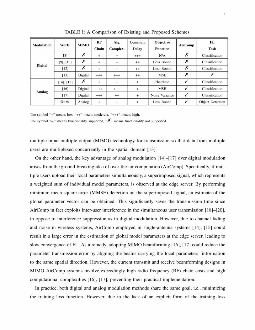
Comparison among four benchmark schemes and the proposed scheme is shown in Fig. 4.
Specifically, the axis of the radar map in Fig. 4a ranges from 0 to 0.3 for MSE (i.e., the objective
function of P), training loss, and test error. The MSE is obtained by averaging over the 400 FL
iterations and the training loss (test error) is obtained when the entire FL procedure terminates.
Since our goal is to minimize all these metrics concurrently, a smaller area indicates better
performance. Firstly, the optimized user transceiver scheme has the largest area, which can be
treated as a worst-case performance bound. This is because the phase shift network at the server
does not align with the users’ channels with the optimized user transceiver scheme. Secondly,
the proposed PAM-based UMAirComp scheme achieves a similar size of triangle as that of the
digital beamforming scheme. This is because for federated learning systems, there is no need
to decode all the local model parameters and more beam directions can be exploited for model
5If the matrix solution to the SDR problem of (14a) is not rank-one, we use the principal component of the obtained matrix
as the phase shift design.
24
0
0.05
0.1
0.15
0.2
0.25
0.3MSE
Training LossTest Error
Optimized User Transceiver [15]
Digital Beamformer Projection [17]
Proposed PAM-based UMAirComp
SDR+CVX [32]
Lower Bound [16]
(a)
0 50 100 150 200 250 300 350 400Number of FL Iterations
0.05
0.1
0.15
0.2
0.25
0.3
0.35
0.4
0.45
0.5
Tra
inin
g Lo
ss
Optimized user transceiver [15]Digital beamformer projection [17]Proposed PAM-based UMAirCompSDR+CVX [32]Lower bound (digital beamformer [16])
(b)
0 50 100 150 200 250 300 350 400Number of FL Iterations
0
0.2
0.4
0.6
0.8
1
Tes
t Err
or
Optimized user transceiver [15]Digital beamformer projection [17]Proposed PAM-baased UMAirCompSDR+CVX [32]Lower bound (digital beamforming [16])
(c)
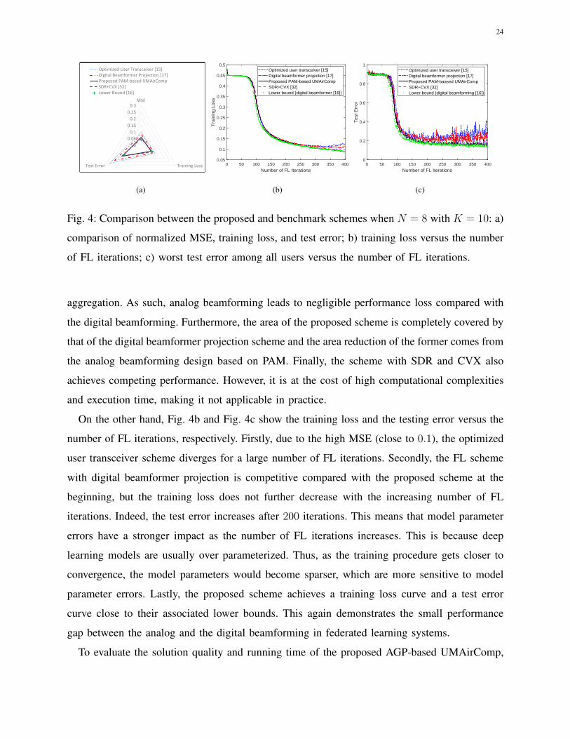
Fig. 4: Comparison between the proposed and benchmark schemes when N = 8 with K = 10: a)
comparison of normalized MSE, training loss, and test error; b) training loss versus the number
of FL iterations; c) worst test error among all users versus the number of FL iterations.
aggregation. As such, analog beamforming leads to negligible performance loss compared with
the digital beamforming. Furthermore, the area of the proposed scheme is completely covered by
that of the digital beamformer projection scheme and the area reduction of the former comes from
the analog beamforming design based on PAM. Finally, the scheme with SDR and CVX also
achieves competing performance. However, it is at the cost of high computational complexities
and execution time, making it not applicable in practice.
On the other hand, Fig. 4b and Fig. 4c show the training loss and the testing error versus the
number of FL iterations, respectively. Firstly, due to the high MSE (close to 0.1), the optimized
user transceiver scheme diverges for a large number of FL iterations. Secondly, the FL scheme
with digital beamformer projection is competitive compared with the proposed scheme at the
beginning, but the training loss does not further decrease with the increasing number of FL
iterations. Indeed, the test error increases after 200 iterations. This means that model parameter
errors have a stronger impact as the number of FL iterations increases. This is because deep
learning models are usually over parameterized. Thus, as the training procedure gets closer to
convergence, the model parameters would become sparser, which are more sensitive to model
parameter errors. Lastly, the proposed scheme achieves a training loss curve and a test error
curve close to their associated lower bounds. This again demonstrates the small performance
gap between the analog and the digital beamforming in federated learning systems.
To evaluate the solution quality and running time of the proposed AGP-based UMAirComp,
25
101 102
Number of Antennas
10-3
10-2
10-1
100
101
102
103
Ave
rage
Run
ning
Tim
e (s
)
SDR+CVXProposed PAM-based UMAirCompLower bound (digital beamforming)Proposed AGP-based UMAirComp
(a)
101 102
Number of Antennas
10-6
10-5
10-4
10-3
10-2
10-1
100
MS
E
Proposed AGP-based UMAirCompProposed PAM-based UMAirCompSDR+CVXLower bound (digital beamforming)
(b)
Dependency
Data Processing
Communication
Module
Scene Generation
Multi-Modal
Sensing Data
Recording
Multi-Sensor
Calibration
Multi-Object
Label
Generation
Multi-Vehicle
Synchronization
& Coordinate
Transformation
Learning
Module
Ubuntu
Algorithm
Module
Object Detection
Local
ParametersState
DesignGlobal
Parameters
CARLA SUMO ROS Pytorch
Dependency
Sparse
Convolution
Region
Proposal
Input
Feature
Extraction
…
Output
(c)
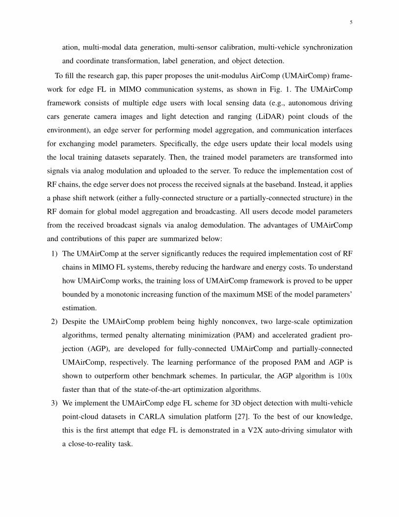
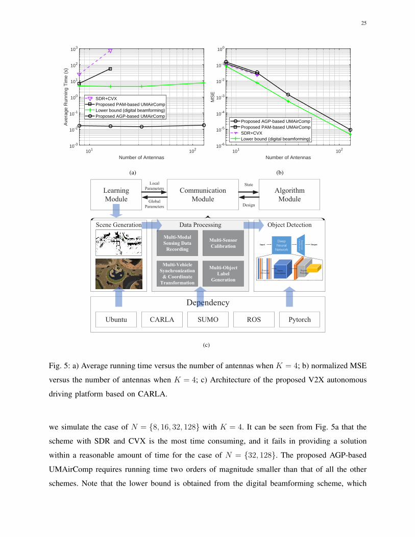
Fig. 5: a) Average running time versus the number of antennas when K = 4; b) normalized MSE
versus the number of antennas when K = 4; c) Architecture of the proposed V2X autonomous
driving platform based on CARLA.
we simulate the case of N = {8, 16, 32, 128} with K = 4. It can be seen from Fig. 5a that the
scheme with SDR and CVX is the most time consuming, and it fails in providing a solution
within a reasonable amount of time for the case of N = {32, 128}. The proposed AGP-based
UMAirComp requires running time two orders of magnitude smaller than that of all the other
schemes. Note that the lower bound is obtained from the digital beamforming scheme, which
26
tackles a less challenging problem without unit-modulus constraints. The AGP algorithm achieves
MSE performance close to that of the proposed PAM algorithm and the lower bound as shown
in Fig. 5b. This indicates that the adopted approximations in the AGP algorithm lead to small
performance loss in practice.
B. UMAirComp for V2X Autonomous Driving
Next, to verify the robustness of the proposed UMAirComp framework in complex learning
tasks, we consider the object detection task for V2X autonomous driving [43]. In particular, we
propose a V2X autonomous driving simulation platform shown in Fig. 5c, which is a virtual-
reality system with close-to-reality environments, interactions, and interfaces. The platform is
developed based on Car Learning to Act (CARLA) [27], Simulation of Urban MObility (SUMO),
Robot Operating System (ROS), and Pytorch in Ubuntu 18.04 with a GeForce GTX 1080 GPU.
The platform consists of learning, communication, and algorithm modules, where the learning
and communication modules interact with each other by exchanging model parameters while
the algorithm module controls the communication module by exchanging system/channel state
information and optimized designs.
For the learning module, it includes scenario generation, data processing, and object detection.
We use CARLA, which is a client-server platform based on Unreal Engine, to construct a high-
fidelity scenario. The “Town02” map is generated with 28 vehicles, including 4 autonomous
vehicles. The entire scenario lasts for 90 seconds and contains 700 frames at each autonomous
vehicle. The first 200 frames are used for training at each vehicle. The latter 500 frames are
used for inference and testing. On the other hand, data processing involves the following steps.
1) Multi-modal sensory data recording. Recording sensory data is implemented based on
Python application programming interfaces (APIs) at the CARLA client [27]. Each au-
tonomous vehicle (Tesla Model 3) is equipped with a GPS, a camera, and a 64-line LiDAR
at 10 Hz. The default LiDAR range is set to 100 m, and its FoV is 90◦ in the front. Each
frame of point cloud is considered as an input data sample dink,l. All the above information
is stored in a sensor file.
2) Multi-sensor calibration. Since each vehicle has three coordinate systems (i.e., LiDAR
coordinate, camera coordinate, and GPS coordinate), we need to compute the rotation
and transition matrices among these coordinate systems [44]. Furthermore, since we have
multiple cameras, we need to compute the ration matrices from the reference camera to
27
other cameras. Lastly, projection matrices are required to associate a point in the 3D space
with a point in the camera image. All the above information is stored in a calibration file.
3) Multi-vehicle synchronization and coordinate transformation. All vehicles should be
synchronized [45]. We adopt the synchronization framework provided by CARLA-SUMO
integration to synchronize the sensors on each vehicle. We exploit the time stamps of the 3D
laser scanner as a reference and consider each spin as a frame. On the other hand, different
vehicles have different local coordinate systems. As such, we use the APIs provided by the
CARLA worlds, maps, and actors to transform these local coordinates to global coordinates.
All the above information is stored in a global coordinate file.
4) Multi-object label generation. The ground truth labels {doutk,l } for object detection should
satisfy the KITTI format. Each label doutk,l consists of 16 elements [44]: 1) category; 2)
boundary or not; 3) occlusion or not; 4) observation angle; 5–6) left top pixel coordinates
in the camera image; 7–8) right bottom pixel coordinates in the camera image; 9) height
of object; 10) width of object; 11) length of object; 12-14) 3D object location in the
camera coordinate system; 15) rotation of object; 16) detection confidence. All the above
information is stored in a label file.6
Finally, the sparsely embedded convolutional detection (SECOND) neural network [25] is
used for object detection on the processed dataset. The local model structure can be found in
[25]. The loss function Θ(dk,l,xk) = fclass (xk,dk,l) + fbox (xk,dk,l) + fsoft (xk,dk,l), where
dk,l =(dink,l,d
outk,l
), fclass is the classification loss, fbox is the box regression loss, and fsoft is
the softmax orientation estimation loss. The SECOND network is trained with a diminishing
learning rate, where the initial learning rate is set to 10−4 and the number of local updates is
E = 1. The average precision at IoU= 0.5 is used for performance evaluation.
For the communication module, the case of N = 500 and K = 4 is simulated. It is assumed
that the sensing datasets are generated and pre-stored at the vehicles before the FL procedure.
The total number of FL iterations is 8, with independently generated channel in each FL iteration.
6In practice, to obtain the training labels of objects, each vehicle broadcasts its ego position and waits for messages from the
nearby infrastructures. Since the infrastructures are fixed at utility poles and connected to servers via wirelines, they have broader
fields of views (FoVs) and deeper neural networks than those of vehicles. Thus, their outputs are more accurate, which can be
transmitted to vehicles via the vehicle-to-infrastructure (V2I) communication and adopted as pseudo labels (i.e., ground-truth
labels with noises).
28
(a) (b) (c) (d)
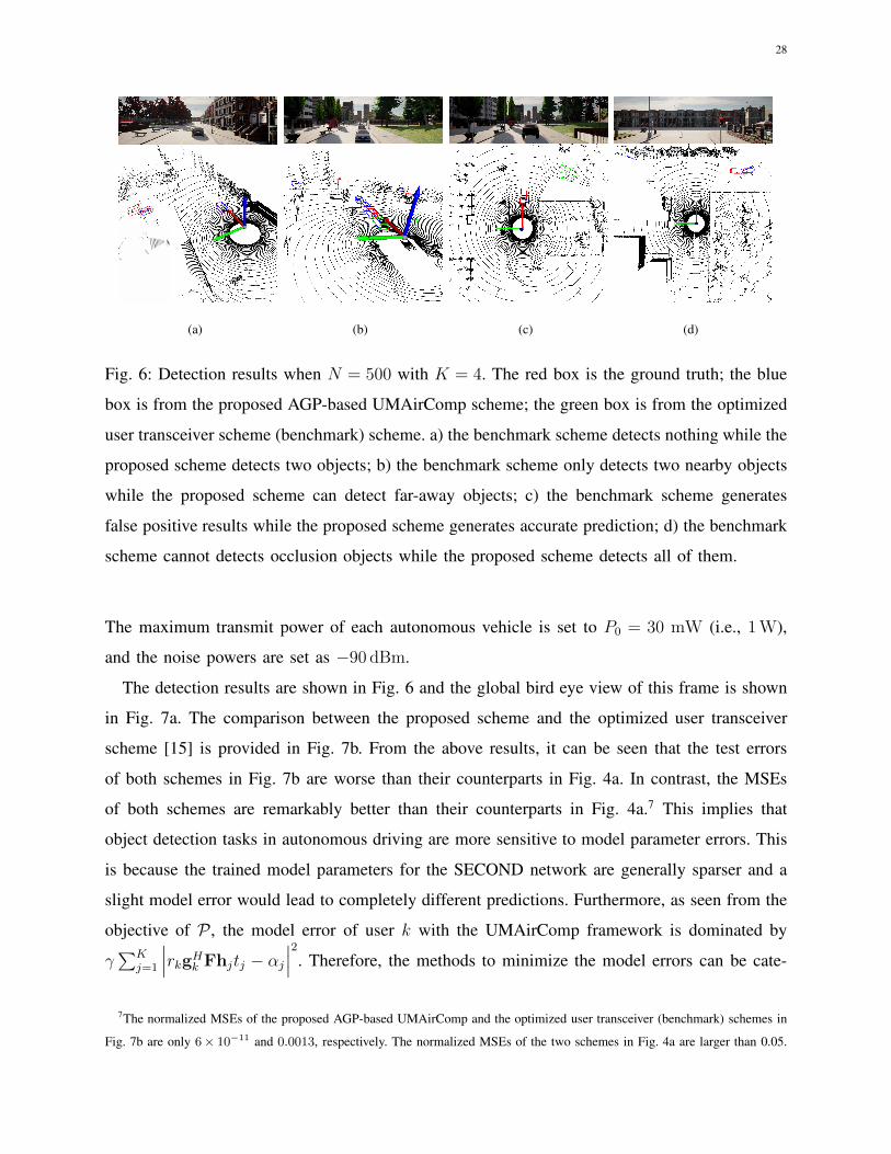
Fig. 6: Detection results when N = 500 with K = 4. The red box is the ground truth; the blue
box is from the proposed AGP-based UMAirComp scheme; the green box is from the optimized
user transceiver scheme (benchmark) scheme. a) the benchmark scheme detects nothing while the
proposed scheme detects two objects; b) the benchmark scheme only detects two nearby objects
while the proposed scheme can detect far-away objects; c) the benchmark scheme generates
false positive results while the proposed scheme generates accurate prediction; d) the benchmark
scheme cannot detects occlusion objects while the proposed scheme detects all of them.
The maximum transmit power of each autonomous vehicle is set to P0 = 30 mW (i.e., 1W),
and the noise powers are set as −90 dBm.
The detection results are shown in Fig. 6 and the global bird eye view of this frame is shown
in Fig. 7a. The comparison between the proposed scheme and the optimized user transceiver
scheme [15] is provided in Fig. 7b. From the above results, it can be seen that the test errors
of both schemes in Fig. 7b are worse than their counterparts in Fig. 4a. In contrast, the MSEs
of both schemes are remarkably better than their counterparts in Fig. 4a.7 This implies that
object detection tasks in autonomous driving are more sensitive to model parameter errors. This
is because the trained model parameters for the SECOND network are generally sparser and a
slight model error would lead to completely different predictions. Furthermore, as seen from the
objective of P , the model error of user k with the UMAirComp framework is dominated by
γ∑K
j=1
∣∣∣rkgHk Fhjtj − αj
∣∣∣2
. Therefore, the methods to minimize the model errors can be cate-
7The normalized MSEs of the proposed AGP-based UMAirComp and the optimized user transceiver (benchmark) schemes in
Fig. 7b are only 6× 10⁻¹¹ and 0.0013, respectively. The normalized MSEs of the two schemes in Fig. 4a are larger than 0.05.
29
Sensing region of
vehicle 1 (Fig. 6a)
Sensing region of
vehicle 4 (Fig. 6d)
Sensing region of
vehicle 3 (Fig. 6c)
Sensing region of
vehicle 2 (Fig. 6b)
Vehicle 1 (Fig. 6a)
Vehicle 4 (Fig. 6d)
Vehicle 3 (Fig. 6c)
Vehicle 2 (Fig. 6b)
Objects
Objects
(a)
(b)
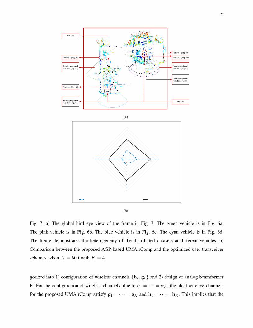
Fig. 7: a) The global bird eye view of the frame in Fig. 7. The green vehicle is in Fig. 6a.
The pink vehicle is in Fig. 6b. The blue vehicle is in Fig. 6c. The cyan vehicle is in Fig. 6d.
The figure demonstrates the heterogeneity of the distributed datasets at different vehicles. b)
Comparison between the proposed AGP-based UMAirComp and the optimized user transceiver
schemes when N = 500 with K = 4.
gorized into 1) configuration of wireless channels {hk, gk} and 2) design of analog beamformer
F. For the configuration of wireless channels, due to α1 = · · · = αK , the ideal wireless channels
for the proposed UMAirComp satisfy g1 = · · · = gK and h1 = · · · = hK . This implies that the
30
UMAirComp should be executed when vehicles are geographically close to each other such that
the magnitudes of {hk, gk} are close. This is the case in vehicle platooning and vehicle parking
scenarios [45]; otherwise, some emerging techniques (e.g., reconfigurable intelligence surfaces
(RIS) [5]) should be adopted to smartly alter the wireless environment. On the other hand, for
the design of beamformers, the key is to align the various channels {hk, gk} to a same direction
and power for decoding superposed signals. This is the case of Fig. 6b, where the proposed
method achieves much larger average precisions than the optimized user transceiver scheme for
all vehicles. Note that the running time of AGP-based UMAirComp is only 0.06 s, which can
be further accelerated via dedicated GPU.
VII. CONCLUSION
This paper proposed the UMAirComp scheme to support simultaneous transmission of local
model parameters in edge federated learning systems. Training loss upper bounds of UMAirComp
were derived, which reveal that the key to minimize FL training loss is to minimize the maximum
MSE among all users. Two low-complexity large-scale optimization algorithms were proposed
to tackle the nonconvex nonsmooth loss bound minimization problem. The performance and
runtime of the UMAirComp framework with the proposed optimization algorithms were verified
using the image classification task. The performance of the proposed framework and algorithms
were also verified in a V2X autonomous driving simulation platform and experimental results
have shown that the object detection precision with the proposed algorithm is significantly higher
than that achieved by benchmark schemes.
APPENDIX A
PROOF OF THEOREM 1
First, let ∆x[i] = x[i+1]k (0)−
[x[i]k (0)− ε∇xΛ
(x[i]k (0)
)]and ‖∆x[i]‖22 can be upper bounded
by
‖∆x[i]‖22 =∥∥∥x[i+1]
k (0)− x[i]k (0) + ε∇xΛ
(x[i]k (0)
)∥∥∥2
2
=∥∥∥x[i+1]
k (0)− θ[i] +K∑
j=1
αjx[i]j (0)− ε
K∑
j=1
αj
|Dj|∑
dj,l∈Dj
∇xΘ(dj,l,x
[i]j (0)
)
− x[i]k (0) + ε∇xΛ(x
[i]k (0))
∥∥∥2
2

31
≤∥∥∥x[i+1]
k (0)− θ[i]∥∥∥2
2+
K∑
j=1
αj
∥∥∥x[i]j (0)− x
[i]k (0)
∥∥∥2
2
+ ε2K∑
j=1
∥∥∥∥∥αj
|Dj|
∑
dj,l∈Dj
∇xΘ(dj,l,x
[i]j (0)
)−∑
dj,l∈Dj
∇xΘ(dj,l,x
[i]k (0)
)
∥∥∥∥∥
2
2
, (48)
where the second equality is obtained from (2) with E = 1 and (10), and the inequality is
obtained due to ‖a1 + a2‖22 ≤ ‖a1‖22 + ‖a2‖22.On the other hand, according to (9), we have
E
[∥∥∥x[i+1]k (0)− θ[i]
∥∥∥2
2
]= MSE
[i]k ,
E
[∥∥∥x[i]k (0)− x
[i]j (0)
∥∥∥2
2
]= E
[∥∥∥x[i]k (0)− θ[i−1] + θ[i−1] − x
[i]j (0)
∥∥∥2
2
]≤ 2MSE
[i]k . (49)
Moreover, according to Assumption 1, we have
E
∥∥∥∥∥
1
|Dj|
∑
dj,l∈Dj
∇xΘ(dj,l,x
[i]j (0)
)−∑
dj,l∈Dj
∇xΘ(dj,l,x
[i]k (0)
)∥∥∥∥∥
2
2
≤ E
[L2‖x[i]
k (0)− x[i]j (0)‖22
]≤ 2L2
MSE[i]k . (50)
Putting (49) and (50) into (48), and according to the expression of ε yields
E[‖∆x[i]‖22
]≤(3 + 2
K∑
j=1
α2j
)max
k=1,··· ,KMSE
[i]k . (51)
Due to 1|Dk|
∑dk,l∈Dk
∇2xΘ(dk,l,x) � LI, we have∇2
xΛ(x) � 1/LI. Based on µI � ∇2
xΛ(x) �
1/LI, the following equations hold [40]:
Λ(x′) ≤ Λ(x) + (x′ − x)T∇Λ(x) + L
2‖x′ − x‖22, (52a)
Λ(x′) ≥ Λ(x) + (x′ − x)T∇Λ(x) + µ
2‖x′ − x‖22. (52b)
Putting x′ = x[i+1]k (0) = x
[i]k (0)− ε∇xΛ
(x[i]k (0)
)+∆x[i] and x = x
[i]k (0) into (52a), we have
Λ(x[i+1]k (0)
)≤ Λ
(x[i]k (0)
)− 1
2L
∥∥∥∇xΛ(x[i]k (0)
)∥∥∥2
2+
L
2‖∆x[i]‖22. (53)
On the other hand, the right hand side of (52b) is minimized at x′ = x − µ−1∇xΛ(x). Putting
this expression and x = x[i]k (0) into (52b) gives
‖∇xΛ(x[i]k (0))‖22 ≥ 2µ
[Λ(x
[i]k (0))− Λ(θ∗)
]. (54)

32
Combining (53) and (54) gives
Λ(x[i+1]k (0))− Λ(x
[i]k (0)) ≤
(1− µ
L
) [Λ(x
[i]k (0))− Λ(θ∗)
]+
L
2‖∆x[i]‖22. (55)
Applying this recursively leads to
Λ(x[i+1]k (0))− Λ(θ∗) ≤
(1− µ
L
)i+1 [Λ(x
[0]k (0))− Λ(θ∗)
]
+
i∑
i′=0
L
2
(1− µ
L
)i−i′
‖∆x[i′]‖22. (56)
Taking expectation on both sides and applying (51), (56) becomes
E
[Λ(x
[i+1]k (0))− Λ(θ∗)
]≤(1− µ
L
)i+1 [Λ(x
[0]k (0))− Λ(θ∗)
]+
i∑
i′=0
A[i′]maxkMSE[i′]k . (57)
Finally, setting, i = R − 1, taking the limit R→ +∞ and using (1− µ/L)R → 0, the proof is
completed.
APPENDIX B
PROOF OF THEOREM 2
Let a[t]k with t = 0, · · · , RE − 1 be the parameter vector at user k such that a
[t]k = x
[i]k (τ) for
t = iE + τ . Define the following virtual sequences {a[t]} as
a[t] =
K∑
k=1
αka[t]k +
K∑
k=1
αkσ[t]k ItmodE=0, (58)
where σ[t]k denotes the model distortion at the k-th user and the t-th iteration, which is upper
bounded by E[‖σ[t]k ‖22] ≤ max∀i,k MSE
[i]k . Based on (58) and equations (2) and (10) in Section
II of the revised manuscript, we have
a[t+1] = a[t] − ε∑K
k=1 |Dk|
K∑
k=1
∑
dk,l∈Dk
∇xkΘ(dk,l,xk)|xk=a
[t]k
+K∑
k=1
αk
(σ
[t+1]k It+1modE=0 − σ
[t]k ItmodE=0
). (59)
Since ε = 2µ(ν+iE+τ)
≤ 14L
and according to [21, Lemma 1], we have
E[‖a[t+1] − θ∗‖22] ≤ (1− µε)E[‖a[t] − θ∗‖22] +K∑
j=1
αjE[‖σ[t+1]j It+1modE=0 − σ
[t]j ItmodE=0‖22]
+2
K
K∑
k=1
E[‖a[t] − a[t]k ‖22] + 6LΓε2. (60)

33
To further bound the right hand side of (60), we notice that for any (k, t),
E[‖σ[t+1]k It+1modE=0 − σ
[t]k ItmodE=0‖22] ≤ E[‖σ[t]
k ‖2] ≤ max∀i,k
MSE[i]k . (E6)
Moreover, based on [22, Lemma A.3], the term E[‖a[t] − a[t]k ‖22] is upper bounded as
E[‖a[t] − a[t]k ‖22] ≤ 4ε2G2E2. (61)
Consequently, the following recursive error bound is obtained
E[‖a[t+1] − θ∗‖22] ≤ (1− µε)E[‖a[t]k − θ∗‖22] + ε2C. (62)
where C is defined in Theorem 2. It can be seen that the above inequality is the same as
equation (B.1) in [22, Lemma A.3]. Following the induction procedure in Appendix B of [22],
the non-recursive error bound is obtained
E[‖a[t] − θ∗‖22] ≤max(4C/µ2, ν‖θ[0] − θ∗‖22)
t+ ν. (E9)
Multiplying 2L on both sides of and using the Lipschitz condition of Λ yield
E[Λ(a[t])
]− Λ(θ∗) ≤ 2LE[‖a[t] − θ∗‖22] ≤
2Lmax(4C, µ2ν‖θ[0] − θ∗‖22)µ2(t+ ν)
, (63)
Substituting a[t]k = x
[R]k (0) and t = ER into (63), the proof is completed.
APPENDIX C
PROOF OF LEMMA 1
Define a surrogate function of h(v) as
g(v,v′) = −K∑
k=1
bk|gHk v|2σ2k
+K∑
k=1
bk (v − v′)H gkgHk (v − v′)
σ2k
. (64)
Since g(v,v′) ≥ h(v), g(v′,v′) = h(v′), and ∇g(v′,v′) ≥ ∇h(v′), with any feasible v(0), every
limit point of the sequence (v(0),v(1), · · · ) generated by the following iteration
v(n+1) = arg min‖v‖22≤β
maxb∈∆
g(v,v(n)) (65)
is the KKT solution to (32). Therefore, to prove the Lemma, it remains to show that U(v′) is
the optimal solution to (65). Specifically, applying the quasi-concave-convex property of (65)
and the general minimax theorem [36], we have
min‖v‖22≤β
maxb∈∆
g(v,v′) = maxb∈∆
min‖v‖22≤β
g(v,v′). (66)

34
Via the Lagrange multiplier method, it can be derived that
arg min||v||22≤β
g(v,v′) =
√βC(v′)b∥∥C(v′)b
∥∥2
. (67)
Putting the above result into g(v,v′), we have
g
( √βC(v′)b∣∣∣∣C(v′)b
∣∣∣∣2
,v′
)= −Φ (v′,b) . (68)
Therefore, the optimal solution of v to (66) (thus (65)) is U(v′) and the proof is completed.
APPENDIX D
PROOF OF LEMMA 2
To prove this theorem, we first introduce the following lemma.
Lemma 4. ( [40, Lemma 1.2.2]) If h(x) is convex and twice differentiable, then h(x) is Lipschitz
smooth with constant L if and only if ∇2h(x) � L I.
Based on Lemma 4 and since Ξ(b) is convex and twice differentiable, it suffices to show
∇2Ξ(b) � LΞ(φ) 1K . In particular, according to (39), the Hessian matrix of Ξ(b) is
∇2Ξ(b) =2√βRe
(CHC
)√
φ2 + ||Cb||22− 2
√β
(√
φ2 + ||Cb||22)3× Re
(CHCb
)[Re
(CHCb
)]H .
Due to Re(CHCb
)[Re
(CHCb
)]H � 0, we can drop the last term to bound ∇2Ξ(b) from
above, which leads to
∇2Ξ(b) � 2√β√
φ2 + ||Cb||22× Re
(CHCb
)� 2√β · λmax
[Re(CHC
)]√
φ2 + ||Cb||22IK , (69)
where the second inequality follows from Re(CHC
)� λmax
[Re(CHC
)]IK .
Now, the only quantity in (69) that is dependent on b is ||Cb||22. To get rid of such dependence,
||Cb||22 is lower bounded by
||Cb||22 = bTCHCb ≥ λmin
(CHC
)× ||b||22. (70)
Finally, using ||b||22 ≥ 1/K due to b ∈ ∆ and Cauchy-Schwarz inequality further leads to
||Cb||22 ≥ λmin
(CHC
)/K. (71)
Replacing ||Cb||22 in (69) with the right hand side of (71), we immediately obtain ∇2Ξ(b) �LΞ(φ) IK .

35
APPENDIX E
PROOF OF THEOREM 4
To prove part (i) of this theorem, notice that Rank (C) = Rank ([g1, · · · , gK ]) due to the
definition of C in (35). As Rank(CHC
)= Rank (C), Rank
(CHC
)= K and λmin
(CHC
)> 0.
Putting λmin
(CHC
)> 0 and φ = 0 into (41), we obtain
LΞ(0) =2√β∣∣∣∣Re
(CHC
) ∣∣∣∣2√
λmin (CHC) /K< +∞. (72)
Next, to prove part (ii), it can be seen that λmin
(CHC
)= 0 if Rank ([g1, · · · , gK ]) 6= K.
Putting this result and φ = 0 into (41), we obtain LΞ(0) = +∞. On the other hand, if φ > 0,
we must have√
φ2 + ||Cb||22 > 0 due to ||Cb||22 ≥ 0. Putting this result into (41), we obtain
LΞ(φ) < +∞ if φ > 0.
Finally, to prove part (iii) of this theorem, we need the following lemma.
Lemma 5. Ξ(b) is bounded as Φ(b) ≤ Ξ(b) ≤ Φ(b) + 2√β φ.
Proof. To prove the left inequality, notice that ||Cb||2 ≤√φ2 + ||Cb||22. Putting this result
into Ξ(b) in (39), we immediately obtain Φ(b) ≤ Ξ(b). On the other hand, to prove the right
inequality, we first compute
Ξ(b)− Φ(b) = 2√
β(√
φ2 + ||Cb||22 −√||Cb||22
). (73)
Then applying the identity√
φ2 + x−√x = φ2√φ2+x+
√x≤ φ, where the inequality is due to the
monotonic decreasing feature of φ2/(√
φ2 + x+√x) with respect to x, the right hand side of
(73) is upper bounded as
2√β(√
φ2 + ||Cb||22 −√||Cb||22
)≤ 2√β φ. (74)
Putting this result into (73), we have Ξ(b)− Φ(b) ≤ 2√β φ.
Now, if an ǫ-optimal solution b′ ∈ ∆ to Q2 is obtained with Ξ(b′) − Ξ(b⋄) ≤ ǫ, then we
must have
Φ(b′) ≤ Ξ(b⋄) + ǫ, (75)
due to Φ(b) ≤ Ξ(b) from the first inequality of Lemma 5. On the other hand, taking the
minimum on both sides of the second inequality of Lemma 5, we have
minb∈∆
Ξ(b) ≤ minb∈∆
Φ(b) + 2√β φ. (76)
36
Putting minb∈∆ Ξ(b) = Ξ(b⋄) and minb∈∆ Φ(b) = Φ(b∗) into (76), (76) becomes Ξ(b⋄) ≤Φ(b∗) + 2
√β φ. Combining this result with (75) leads to Φ(b′) ≤ Φ(b∗) + 2
√β φ+ ǫ, and part
(iii) of this theorem is proved.
REFERENCES
[1] Y. LeCun, Y. Bengio, and G. Hinton, “Deep learning,” Nature, vol. 521, pp. 436–444, May 2015.
[2] W. Saad, M. Bennis, and M. Chen, “A vision of 6G wireless systems: Applications, trends, technologies, and open research
problems,” IEEE Netw., vol. 34, no. 3, pp. 134–142, May–Jun. 2020.
[3] S. Yu, X. Chen, L. Yang, D. Wu, M. Bennis, and J. Zhang, “Intelligent edge: Leveraging deep imitation learning for
mobile edge computation offloading,” IEEE Wireless Commun. vol. 27, no. 1, pp. 92–99, Feb. 2020.
[4] S. Wang, Y.-C. Wu, M. Xia, R. Wang, and H. V. Poor, “Machine intelligence at the edge with learning centric power
allocation,” IEEE Trans. Wireless Commun., vol. 19, no. 11, pp. 7293–7308, Nov. 2020.
[5] S. Huang, S. Wang, R. Wang, M. Wen, and K. Huang, “Reconfigurable intelligent surface assisted mobile edge computing
with heterogeneous learning tasks,” IEEE Trans. Cognitive Commun. Networking, vol. 7, no. 2, pp. 369–382, Jun. 2021.
[6] Google Research, [Online]. Available: https://ai.googleblog.com/2017/04/federated-learning-collaborative.html.
[7] Y. Shi, K. Yang, T. Jiang, J. Zhang, and K. B. Letaief, “Communication-efficient edge AI: Algorithms and systems,” IEEE
Commun. Surveys Tuts., vol. 22, no. 4, pp. 2167–2191, Fourthquarter 2020.
[8] H. B. McMahan, E. Moore, D. Ramage, S. Hampson, and B. Arcas, “Communication-efficient learning of deep networks
from decentralized data,” in Proc. AISTATS, Fort Lauderdale, Florida, Apr. 2017.
[9] S. Wang, T. Tuor, T. Salonidis, K. K. Leung, C. Makaya, T. He, and K. Chan, “Adaptive federated learning in resource
constrained edge computing systems,” IEEE J. Sel. Areas Commun., vol. 37, no. 6, pp. 1205–1221, Jun. 2019.
[10] M. Chen, Z. Yang, W. Saad, C. Yin, H. V. Poor, and S. Cui, “A joint learning and communications framework for federated
learning over wireless networks,” IEEE Trans. Wireless Commun., vol. 20, no. 1, pp. 269–283, Jan. 2021.
[11] T. Zen, O. Semiari, M. Mozaffari, M. Chen, W. Saad, and M. Bennis, “Federated learning in the sky: Joint power allocation
and scheduling with UAV swarms,” in Proc. IEEE ICC, Dublin, Ireland, Jun. 2020.
[12] Y. Du, S. Yang, and K. Huang, “High-dimensional stochastic gradient quantization for communication-efficient edge
learning,” IEEE Trans. Signal Process., vol. 68, pp. 2128–2142, Mar. 2020.
[13] T. T. Vu, D. T. Ngo, N. H. Tran, H. Q. Ngo, M. N. Dao, and R. H. Middleton, “Cell-free massive MIMO for wireless
federated learning,” IEEE Trans. Wireless Commun., vol. 19, no. 10, pp. 6377–6392, Oct. 2020.
[14] M. M. Amiri and D. Gunduz, “Machine learning at the wireless edge: Distributed stochastic gradient descent over-the-air,”
IEEE Trans. Signal Process., vol. 68, pp. 2155–2169, Mar. 2020.
[15] G. Zhu, Y. Wang, and K. Huang, “Broadband analog aggregation for low-latency federated edge learning,” IEEE Trans.
Wireless Commun., vol. 19, no. 1, pp. 491–506, Jan. 2020.
[16] K. Yang, T. Jiang, Y. Shi, and Z. Ding, “Federated learning via over-the-air computation,” IEEE Trans. Wireless Commun.
vol. 19, no. 3, pp. 2022–2035, Mar. 2020.
[17] H. Guo, A. Liu, and V. K. N. Lau, “Analog gradient aggregation for federated learning over wireless networks: Customized
design and convergence analysis,” IEEE Internet of Things J., vol. 8, no. 1, pp. 197–210, Jan. 2021.
[18] L. Chen, N. Zhao, Y. Chen, F. R. Yu, and G. Wei, “Toward optimal rate-delay tradeoff for computation over multiple
access channel,” IEEE Trans. Commun., vol. 69, no. 7, pp. 4335–4346, Jul. 2021.
[19] L. Chen, N. Zhao, Y. Chen, X. Qin, and F. R. Yu, “Computation over MAC: Achievable function rate maximization in
wireless networks,” IEEE Trans. Commun., vol. 68, no. 9, pp. 5446–5459, Sep. 2020.

37
[20] H. Hellstrom, J. Mairton, B. da Silva Jr, V. Fodor, and C. Fischione, “Wireless for machine learning,” [Online]. Available:
https://arxiv.org/abs/2008.13492, 2020.
[21] X. Li, K. Huang, W. Yang, S. Wang, and Z. Zhang, “On the convergence of fedavg on non-iid data,” in Proc. ICLR, Addis
Ababa, Ethiopia, Apr. 2020.
[22] T. Sery, N. Shlezinger, K. Cohen, and Y. C. Eldar, “Over-the-air federated learning from heterogeneous data,” IEEE Trans.
Signal Process., vol. 69, pp. 3796–3811, Jun. 2021.
[23] F. Sohrabi and W. Yu, “Hybrid digital and analog beamforming design for large-scale antenna arrays,” IEEE J. Sel. Topics
Signal Process., vol. 10, no. 3, pp. 501–513, Apr. 2016.
[24] V. Venkateswaran and A. J. van der Veen, “Analog beamforming in MIMO communications with phase shift networks and
online channel estimation,” IEEE Trans. Signal Process., vol. 58, no. 8, pp. 4131–4143, Aug. 2010.
[25] Y. Yan, Y. Mao, and B. Li, “SECOND: Sparsely embedded convolutional detection,” Sensors, vol. 18, no. 10, pp. 3337,
Oct. 2018.
[26] S. Shi, Z. Wang, J. Shi, X. Wang, and H. Li, “From points to parts: 3D object detection from point cloud with part-aware
and part-aggregation network,” IEEE Trans. Pattern Anal. Mach. Intell., vol. 43, no. 8, pp. 2647–2664, Aug. 2021.
[27] A. Dosovitskiy, G. Ros, F. Codevilla, A. Lopez, and V. Koltun, “CARLA: An open urban driving simulator,” in Proc. The
1st Annual Conference on Robot Learning, 2017, pp. 1–16.
[28] M. P. Friedlander and M. Schmidt, “Hybrid deterministic-stochastic methods for data fitting,” SIAM J. Sci. Comput., vol. 34,
no. 3, pp. 1380–1405, May 2012.
[29] A. Beck, “On the convergence of alternating minimization for convex programming with applications to iteratively
reweighted least squares and decomposition schemes,” SIAM J. Optimiz., vol. 25, no. 1, pp. 185–209, 2015.
[30] X. Zhang, Matrix Analysis and Applications. Beijing, China: Tsinghua Univ. Press, 2004.
[31] Y. Wang, J. Yang, W. Yin, and Y. Zhang, “A new alternating minimization algorithm for total variation image
reconstruction,” SIAM J. Imaging Sciences, vol. 1, no. 3, pp. 248–272, 2008.
[32] S. Boyd and L. Vandenberghe, Convex Optimization. Cambridge, U.K.: Cambridge Univ. Press, 2004.
[33] S. Wang, L. Cheng, M. Xia, and Y.-C. Wu, “Massive MIMO multicast beamforming via accelerated random coordinate
descent,” in Proc. IEEE ICASSP’19, Brighton, UK, May 2019, pp. 4494–4498.
[34] N. Parikh and S. Boyd, “Proximal algorithms,” Foundations and Trends in Optimization, vol. 1, no. 3, pp. 127–239, 2014.
[35] Y. Sun, P. Babu, and D. P. Palomar, “Majorization-minimization algorithms in signal processing, communications, and
machine learning,” IEEE Trans. Signal Process., vol. 65, no. 3, pp. 794–816, Feb. 2017.
[36] M. Sion, “On general minimax theorems,” Pacific J. Math., vol. 8, no. 1, pp. 171–176, 1958.
[37] Y. Nesterov, “Smooth minimization of non-smooth functions,” Math. Program., vol. 103, no. 1, pp. 127–152, May 2005.
[38] W. Su, S. Boyd, and E. J. Candes, “A differential equation for modeling Nesterov’s accelerated gradient method: Theory
and insights”, J. Mach. Learn. Res., vol. 17, no. 153, pp. 1–43, Sep. 2016.
[39] A. Beck and M. Teboulle, “A fast iterative shrinkage-thresholding algorithm for linear inverse problems,” SIAM J. Imaging
Sci., vol. 2, no. 1, pp. 183–202, Mar. 2009.
[40] Y. Nesterov, Introductory Lectures on Convex Optimization: A Basic Course. Applied Optimization. Springer, 2004.
[41] L. Condat, “Fast projection onto the simplex and the l1 ball,” Math. Program., vol. 158, no. 1, pp. 575–585, Jul. 2016.
[42] L. Deng, “The MNIST database of handwritten digit images for machine learning research,” IEEE Signal Process. Mag.,
vol. 29, no. 6, pp. 141–142, Nov. 2012.
[43] Z. Zhang, S. Wang, Y. Hong, L. Zhou, and Q. Hao, “Distributed dynamic map fusion via federated learning for intelligent
networked vehicles,” in Proc. IEEE ICRA, Xi’an, China, May–Jun. 2021, pp. 953 959.

38
[44] A. Geiger, P. Lenz, C. Stiller, and R. Urtasun , “Vision meets robotics: The KITTI dataset,” Int. J. Rob. Res., vol. 32,
no. 11, pp. 1231–1237, 2013.
[45] A. Eskandarian, C. Wu, and C. Sun, “Research advances and challenges of autonomous and connected ground vehicles,”
IEEE Trans. Intell. Transp. Syst., vol. 22, no. 2, pp. 683 –711, Feb. 2021.
[46] S. Wang, D. Li, R. Wang, Q. Hao, Y.-C. Wu, and D. W. K. Ng, “Unit-modulus wireless federated learning
via penalty alternating minimization,” in Proc. IEEE GLOBECOM, Madrid, Spain, Dec. 2021. [Online]. Available:
https://arxiv.org/abs/2108.13669.pdf.


![Differentially Private Asynchronous Federated Learning for Mobile Edge Computing …folk.uio.no/yanzhang/IEEETIILYL1.pdf · 2020-01-13 · Federated Learning [12], [13] can introduce](https://cdn.vdocuments.net/doc/165x107/5f020db37e708231d4025841/differentially-private-asynchronous-federated-learning-for-mobile-edge-computing.jpg)


