EGR 106 – Week 2 – Arrays & Scripts
Brief review of last week Arrays:
– Concept– Construction– Addressing
Scripts and the editor Audio arrays Textbook 2.1-2.6, chapter 4.1-4.3

Review of Last Week
Variables: placeholders for numerical data– equal sign is an assignment operator – naming restrictions (not pi, etc. ) – can be complex valued ( x = 3 + 7 i )
Basic math on numbers and variables:
+ – * / ^

Array Concept
The fundamental data unit in Matlab– Rectangular collection of data– All variables are considered to be arrays
Data values organized into rows and columns
4 5 3 91 0 4 6 6 2 01 8 -3 2 0
y ie ld =
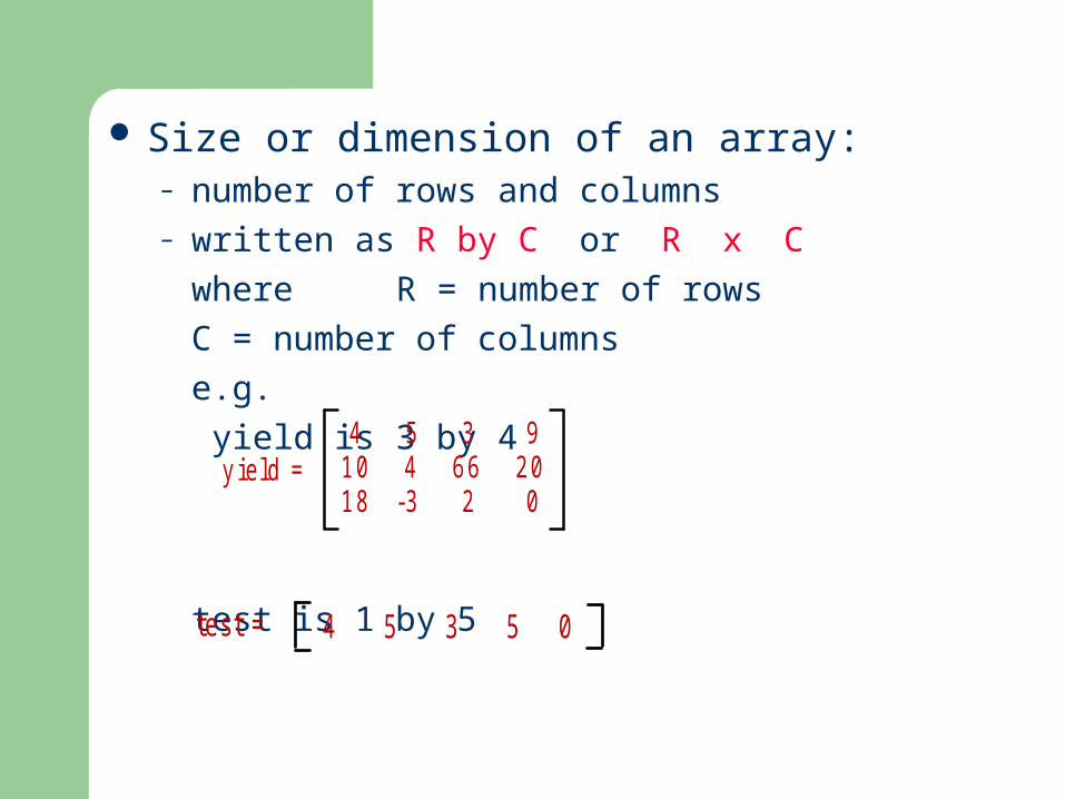
Size or dimension of an array:– number of rows and columns– written as R by C or R x C
where R = number of rows
C = number of columns
e.g.
yield is 3 by 4
test is 1 by 5
4 5 3 91 0 4 6 6 2 01 8 -3 2 0
y ie ld =
4 5 3 5 0 te s t =
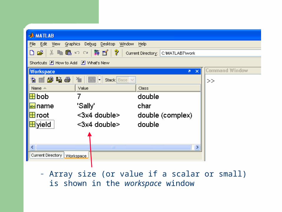
– Array size (or value if a scalar or small) is shown in the workspace window
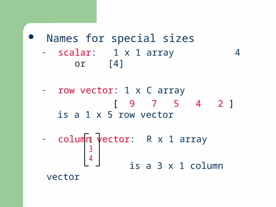
Names for special sizes– scalar: 1 x 1 array 4 or [4]
– row vector: 1 x C array
[ 9 7 5 4 2 ] is a 1 x 5 row vector
– column vector: R x 1 array
is a 3 x 1 column vector
134

– matrix: R x C array with R > 1, C > 1
If R = C square matrix– each row must have the same number of entries
If R = C = 0 null matrix [ ] (a pair of empty brackets)
4 5 31 0 4 6 61 8 -3 2

Array Construction
Direct specification:– Name followed by an equal sign ( = ),
just like variables– List values within a pair of brackets ( [ ] )– Enter data one row at a time
left to right, top to bottom order space or comma between the values rows separated by semicolons or the enter key
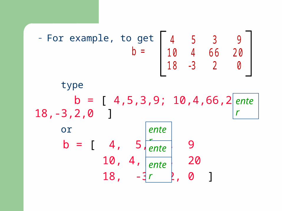
– For example, to get
type
b = [ 4,5,3,9; 10,4,66,20; 18,-3,2,0 ]
or
b = [ 4, 5, 3, 9
10, 4, 66, 20
18, -3, 2, 0 ]
4 5 3 91 0 4 6 6 2 01 8 -3 2 0
b =
enter
enter
enter
enter

– Can use simple math operations as well as numerics as the entries:
– Note the common format of all entries in the response (exp(1) = e = 2.71828, log10(100) = 2, 2-12 = 0.00024414)
– MATLAB scales the exponent to the largest entry !!

– This scaling is sometimes deceptive:
Not really zero
Really zero

Concatenation – gluing arrays together
if a = [ 1 2 3 ] b = [ 4 5 6 ]
– Attaching left to right – use a comma
[ a, b ]
– Attaching top to bottom – use a semicolon
[ a; b ] 1 2 3 4 5 6
1 2 3 4 5 6
semicolon
comma

– Note that sizes must match for this to work:
if a = [ 1 2 3 ] then
[ a, b ] = ?? [ a; b ] = ??
– Size needs for concatenation:# of rows the same for side by side (comma)# of columns the same for top to bottom
(semicolon)
4 51 0 4
b =

Evenly spaced vectors – the colon operator
first : increment : maximum
yields a row vector of equally spaced values– examples:
0 : 2 : 10 [ 0 2 4 6 8 10 ]
1 : 5 [ 1 2 3 4 5 ]
7 : -2 : -3 [ 7 5 3 1 -1 -3 ]
1 : 2 : 8 [ 1 3 5 7 ] – default for increment is 1
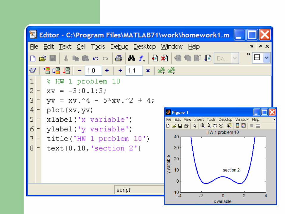
Note – does not hit 8!!Recall Assignment 1, #10
xv = –3:0.1:3;

Addressing
We indicate a particular element within an array by it’s row/column position:
– use parentheses after the array name– e.g. yield(2,4)
4 5 3 91 0 4 6 6 2 01 8 -3 2 0
y ie ld =

Used to read a value from an array (right hand side of = )
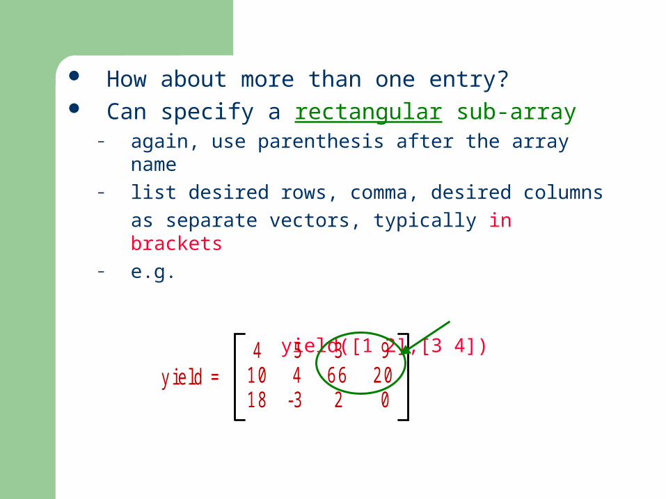
How about more than one entry? Can specify a rectangular sub-array
– again, use parenthesis after the array name– list desired rows, comma, desired columns
as separate vectors, typically in brackets – e.g.
yield([1 2],[3 4])
4 5 3 91 0 4 6 6 2 01 8 -3 2 0
y ie ld =
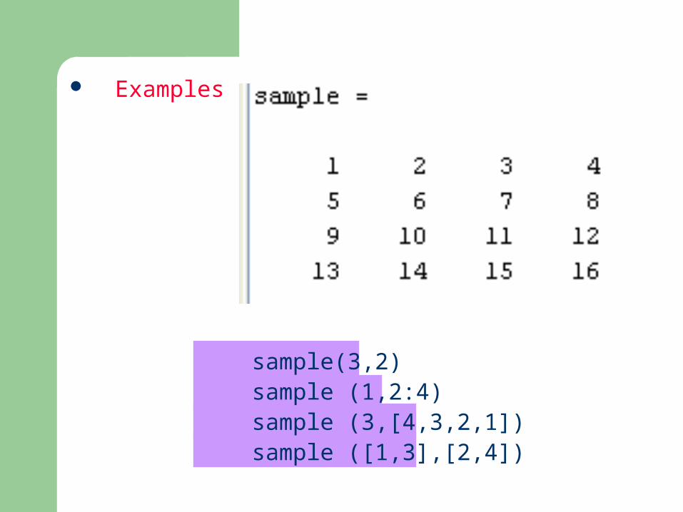
Examples
sample(3,2) sample (1,2:4)sample (3,[4,3,2,1])sample ([1,3],[2,4])

Used to read a sub-array ( rhs of =)
Note – scalar row choice does not need brackets!

Avoid some common addressing errors:
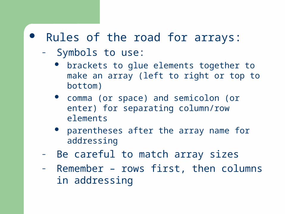
Rules of the road for arrays:– Symbols to use:
brackets to glue elements together to make an array (left to right or top to bottom)
comma (or space) and semicolon (or enter) for separating column/row elements
parentheses after the array name for addressing
– Be careful to match array sizes– Remember – rows first, then columns in
addressing
Scripts – Simple Programs
So far, commands have been typed in the command window: – Executed by pressing “enter”– Edited using the arrow keys or
the history window

Script (m-file) Concept
A file containing Matlab commands – Can be re-executed – Is easily changed/modified or e-mailed to someone
Commands are executed one by one, sequentially– File is executed by typing its name (without .m)– Results appear in the command window (or use ; )
Can be created using any text editor – .m extension– Listed in Current Directory window


Matlab’s Built-in, Color Editor: – Can create a new file
or open an existing
M file (icons or click
on file name)– Color used to aid in
file creation
(command types,
typos, etc.)

– typical Windows menu– line numbers – “run” button or F5 – debug capability
– comment lines – note use of semicolons– note use of colors
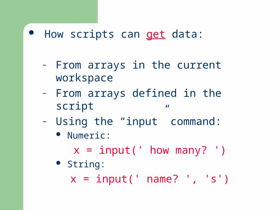
How scripts can get data:
– From arrays in the current workspace– From arrays defined in the script– Using the “input” command:
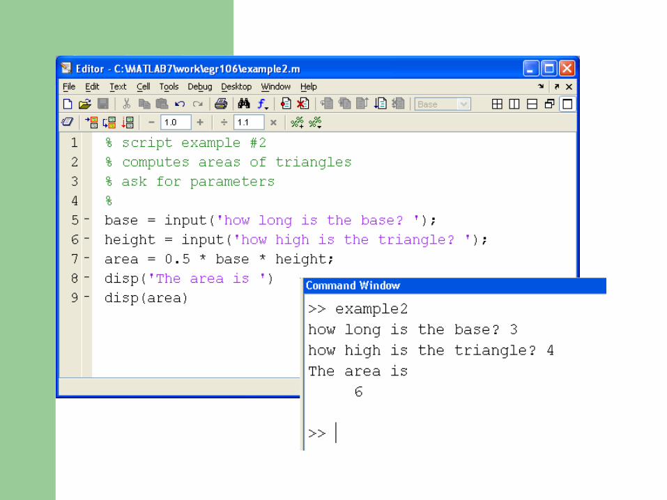
Numeric:
x = input(' how many? ') String:
x = input(' name? ', 's')

How scripts can show data:
– Command of the array name– Using the display command:
Existing array (a single array only – if necessary, use [ ] !!)
disp(x) or disp([x y]) Text
disp(' The task is done ')

Example:
Note that disp shortens the resulting output by dropping the array name and removing blank lines
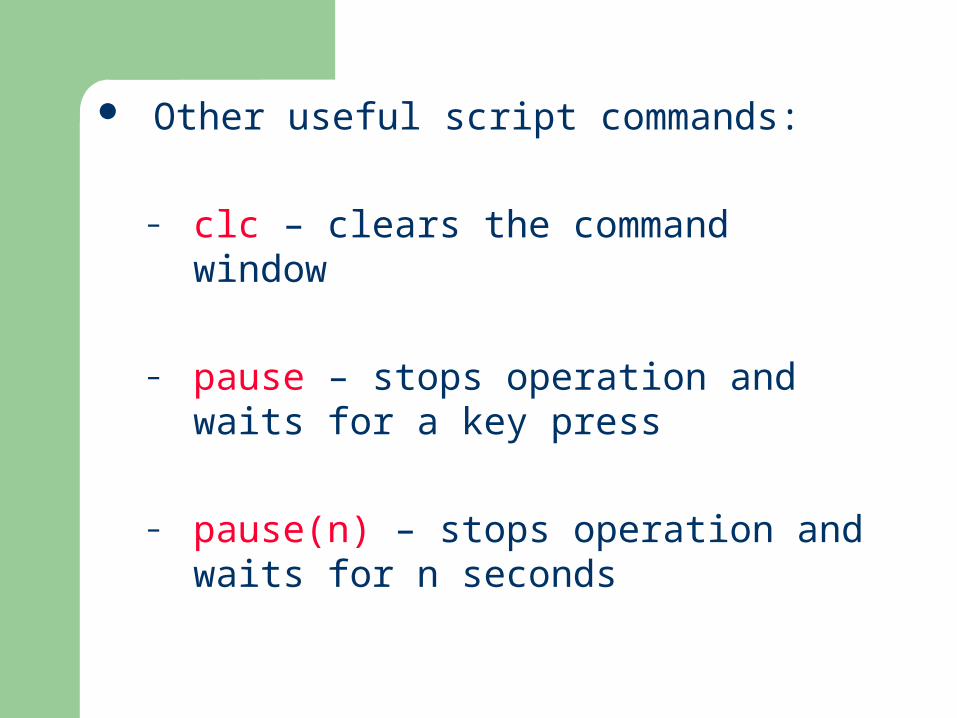
Other useful script commands:
– clc – clears the command window
– pause – stops operation and waits for a key press
– pause(n) – stops operation and waits for n seconds
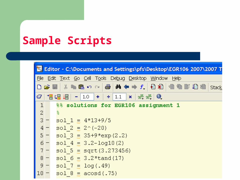
Sample Scripts

Audio Arrays (not in the book!)
MatLab can interface to microphones and speakers through the computer’s sound card (sampled and digitized) ….e.g. “maple”
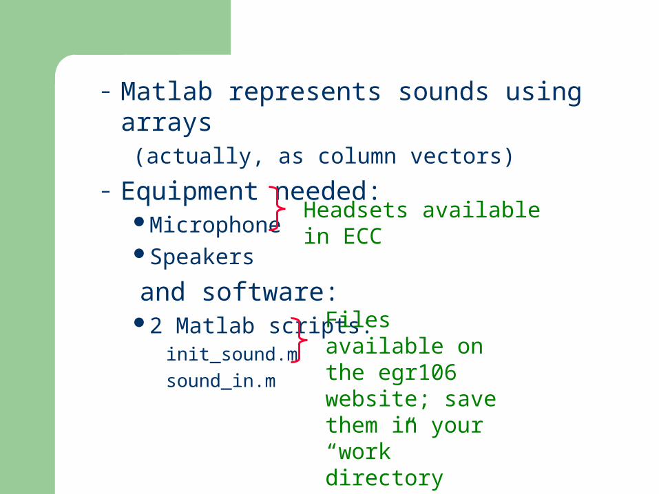
– Matlab represents sounds using arrays (actually, as column vectors)
– Equipment needed:MicrophoneSpeakers
and software:2 Matlab scripts:
init_sound.m
sound_in.m
Headsets available in ECC
Files available on the egr106 website; save them in your “work” directory

– How to use them: Connect headset (is it muted?)Type init_sound at the command prompt (only
needed once per session)Type sound_in at the command prompt to
record 1 second of sound (waits for your input)
generates array named “data”Type sound(data,10000) at the prompt to
play array “data” – Can plot “data”, manipulate “data” before replaying,
etc.
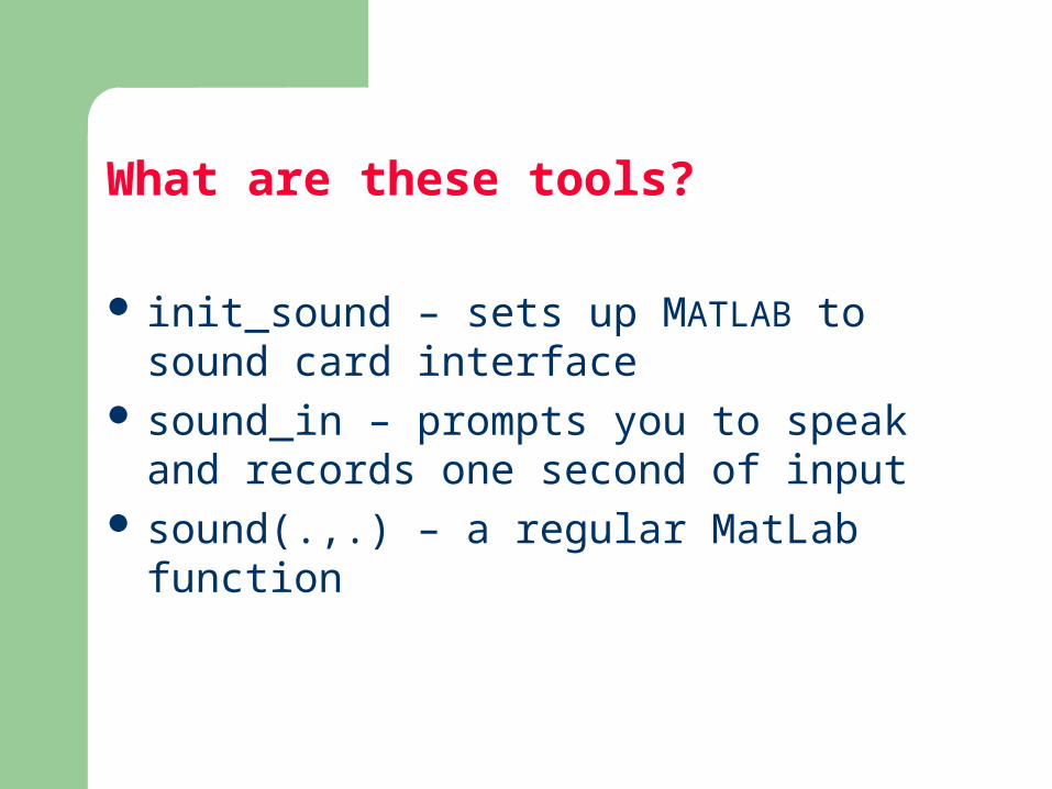
init_sound – sets up MATLAB to sound card interface
sound_in – prompts you to speak and records one second of input
sound(.,.) – a regular MatLab function
What are these tools?


•Time Sampling – Speech

•Whistling a Scale

•Normal versus too loud an input


