This is page iPrinter: Opaque this
Elementary Number Theory
William Stein
October 2005

ii
To my students and my wife, Clarita Lefthand.
This is page iiiPrinter: Opaque this
Contents
Preface 3
1 Prime Numbers 51.1 Prime Factorization . . . . . . . . . . . . . . . . . . . . . . 51.2 The Sequence of Prime Numbers . . . . . . . . . . . . . . . 131.3 Exercises . . . . . . . . . . . . . . . . . . . . . . . . . . . . 19
2 The Ring of Integers Modulo n 212.1 Congruences Modulo n . . . . . . . . . . . . . . . . . . . . . 212.2 The Chinese Remainder Theorem . . . . . . . . . . . . . . . 272.3 Quickly Computing Inverses and Huge Powers . . . . . . . . 292.4 Finding Primes . . . . . . . . . . . . . . . . . . . . . . . . . 332.5 The Structure of (Z/pZ)∗ . . . . . . . . . . . . . . . . . . . 342.6 Exercises . . . . . . . . . . . . . . . . . . . . . . . . . . . . 38
3 Public-Key Cryptography 433.1 The Diffie-Hellman Key Exchange . . . . . . . . . . . . . . 463.2 The RSA Cryptosystem . . . . . . . . . . . . . . . . . . . . 513.3 Attacking RSA . . . . . . . . . . . . . . . . . . . . . . . . . 543.4 Exercises . . . . . . . . . . . . . . . . . . . . . . . . . . . . 58
4 Quadratic Reciprocity 594.1 Statement of the Quadratic Reciprocity Law . . . . . . . . 604.2 Euler’s Criterion . . . . . . . . . . . . . . . . . . . . . . . . 62
Contents 1
4.3 First Proof of Quadratic Reciprocity . . . . . . . . . . . . . 634.4 A Proof of Quadratic Reciprocity Using Gauss Sums . . . . 684.5 Finding Square Roots . . . . . . . . . . . . . . . . . . . . . 724.6 Exercises . . . . . . . . . . . . . . . . . . . . . . . . . . . . 74
5 Continued Fractions 775.1 Finite Continued Fractions . . . . . . . . . . . . . . . . . . 785.2 Infinite Continued Fractions . . . . . . . . . . . . . . . . . . 835.3 The Continued Fraction of e . . . . . . . . . . . . . . . . . . 885.4 Quadratic Irrationals . . . . . . . . . . . . . . . . . . . . . . 915.5 Recognizing Rational Numbers . . . . . . . . . . . . . . . . 965.6 Sums of Two Squares . . . . . . . . . . . . . . . . . . . . . 975.7 Exercises . . . . . . . . . . . . . . . . . . . . . . . . . . . . 100
6 Elliptic Curves 1036.1 The Definition . . . . . . . . . . . . . . . . . . . . . . . . . 1036.2 The Group Structure on an Elliptic Curve . . . . . . . . . . 1046.3 Integer Factorization Using Elliptic Curves . . . . . . . . . 1076.4 Elliptic Curve Cryptography . . . . . . . . . . . . . . . . . 1136.5 Elliptic Curves Over the Rational Numbers . . . . . . . . . 1176.6 Exercises . . . . . . . . . . . . . . . . . . . . . . . . . . . . 121
7 Computational Number Theory 1257.1 Prime Numbers . . . . . . . . . . . . . . . . . . . . . . . . . 1277.2 The Ring of Integers Modulo n . . . . . . . . . . . . . . . . 1337.3 Public-Key Cryptography . . . . . . . . . . . . . . . . . . . 1417.4 Quadratic Reciprocity . . . . . . . . . . . . . . . . . . . . . 1477.5 Continued Fractions . . . . . . . . . . . . . . . . . . . . . . 1507.6 Elliptic Curves . . . . . . . . . . . . . . . . . . . . . . . . . 1547.7 Exercises . . . . . . . . . . . . . . . . . . . . . . . . . . . . 162
Answers and Hints 165
References 173

2 Contents
This is page 3Printer: Opaque this
Preface
This is a textbook about prime numbers, congruences, basic public-keycryptography, quadratic reciprocity, continued fractions, elliptic curves, andnumber theory algorithms. We assume the reader has some familiarity withgroups, rings, and fields, and for Chapter 7 some programming experience.This book grew out of an undergraduate course that the author taught atHarvard University in 2001 and 2002.
Notation and Conventions. We let N = {1, 2, 3, . . .} denote the naturalnumbers, and use the standard notation Z, Q, R, and C for the rings ofinteger, rational, real, and complex numbers, respectively. In this book wewill use the words proposition, theorem, lemma, and corollary as follows.Usually a proposition is a less important or less fundamental assertion, atheorem a deeper culmination of ideas, a lemma something that we willuse later in this book to prove a proposition or theorem, and a corollaryan easy consequence of a proposition, theorem, or lemma.
Acknowledgements. Brian Conrad and Ken Ribet made a large numberof clarifying comments and suggestions throughout the book. BaurzhanBektemirov, Lawrence Cabusora, and Keith Conrad read drafts of this bookand made many comments. Frank Calegari used the course when teachingMath 124 at Harvard, and he and his students provided much feedback.Noam Elkies made comments and suggested Exercise 4.5. Seth Kleinermanwrote a version of Section 5.3 as a class project. Samit Dasgupta, GeorgeStephanides, Kevin Stern, and Heidi Williams all suggested corrections. I
4 Contents
also benefited from conversations with Henry Cohn and David Savitt. Iused Emacs, LATEX, and Python in the preparation of this book.
This is page 5Printer: Opaque this
1Prime Numbers
In Section 1.1 we describe how the integers are built out of the primenumbers 2, 3, 5, 7, 11, . . .. In Section 1.2 we discuss theorems about the setof primes numbers, starting with Euclid’s proof that this set is infinite,then explore the distribution of primes via the prime number theorem andthe Riemann Hypothesis (without proofs).
1.1 Prime Factorization
1.1.1 Primes
The set of natural numbers is
N = {1, 2, 3, 4, . . .},
and the set of integers is
Z = {. . . ,−2,−1, 0, 1, 2, . . .}.
Definition 1.1.1 (Divides). If a, b ∈ Z we say that a divides b, writtena | b, if ac = b for some c ∈ Z. In this case we say a is a divisor of b. We saythat a does not divide b, written a ∤ b, if there is no c ∈ Z such that ac = b.
For example, we have 2 | 6 and −3 | 15. Also, all integers divide 0, and 0divides only 0. However, 3 does not divide 7 in Z.
Remark 1.1.2. The notation b.: a for “b is divisible by a” is common in
Russian literature on number theory.
6 1. Prime Numbers
Definition 1.1.3 (Prime and Composite). An integer n > 1 is primeif it the only positive divisors of n are 1 and n. We call n composite if n isnot prime.
The number 1 is neither prime nor composite. The first few primes of Nare
2, 3, 5, 7, 11, 13, 17, 19, 23, 29, 31, 37, 41, 43, 47, 53, 59, 61, 67, 71, 73, 79, . . . ,
and the first few composites are
4, 6, 8, 9, 10, 12, 14, 15, 16, 18, 20, 21, 22, 24, 25, 26, 27, 28, 30, 32, 33, 34, . . . .
Remark 1.1.4. J. H. Conway argues in [Con97, viii] that −1 should beconsidered a prime, and in the 1914 table [Leh14], Lehmer considers 1 tobe a prime. In this book we consider neither −1 nor 1 to be prime.
Every natural number is built, in a unique way, out of prime numbers:
Theorem 1.1.5 (Fundamental Theorem of Arithmetic). Every nat-ural number can be written as a product of primes uniquely up to order.
Note that primes are the products with only one factor and 1 is theempty product.
Remark 1.1.6. Theorem 1.1.5, which we will prove in Section 1.1.4, is trick-ier to prove than you might first think. For example, unique factorizationfails in the ring
Z[√−5] = {a + b
√−5 : a, b ∈ Z} ⊂ C,
where 6 factors into irreducible elements in two different ways:
2 · 3 = 6 = (1 +√−5) · (1 −
√−5).
1.1.2 The Greatest Common Divisor
We will use the notion of greatest common divisor of two integers to provethat if p is a prime and p | ab, then p | a or p | b. Proving this is the keystep in our proof of Theorem 1.1.5.
Definition 1.1.7 (Greatest Common Divisor). Let
gcd(a, b) = max {d ∈ Z : d | a and d | b} ,
unless both a and b are 0 in which case gcd(0, 0) = 0.
For example, gcd(1, 2) = 1, gcd(6, 27) = 3, and for any a, gcd(0, a) =gcd(a, 0) = a.
If a 6= 0, the greatest common divisor exists because if d | a then d ≤ a,and there are only a positive integers ≤ a. Similarly, the gcd exists whenb 6= 0.
1.1 Prime Factorization 7
Lemma 1.1.8. For any integers a and b we have
gcd(a, b) = gcd(b, a) = gcd(±a,±b) = gcd(a, b − a) = gcd(a, b + a).
Proof. We only prove that gcd(a, b) = gcd(a, b − a), since the other casesare proved in a similar way. Suppose d | a and d | b, so there exist integersc1 and c2 such that dc1 = a and dc2 = b. Then b−a = dc2−dc1 = d(c2−c1),so d | b − a. Thus gcd(a, b) ≤ gcd(a, b − a), since the set over which we aretaking the max for gcd(a, b) is a subset of the set for gcd(a, b − a). Thesame argument with a replaced by −a and b replaced by b− a, shows thatgcd(a, b − a) = gcd(−a, b − a) ≤ gcd(−a, b) = gcd(a, b), which proves thatgcd(a, b) = gcd(a, b − a).
Lemma 1.1.9. Suppose a, b, n ∈ Z. Then gcd(a, b) = gcd(a, b − an).
Proof. By repeated application of Lemma 1.1.8, we have
gcd(a, b) = gcd(a, b − a) = gcd(a, b − 2a) = · · · = gcd(a, b − 2n).
Assume for the moment that we have already proved Theorem 1.1.5.A natural (and naive!) way to compute gcd(a, b) is to factor a and b asa product of primes using Theorem 1.1.5; then the prime factorization ofgcd(a, b) can read off from that of a and b. For example, if a = 2261 andb = 1275, then a = 7 · 17 · 19 and b = 3 · 52 · 17, so gcd(a, b) = 17. It turnsout that the greatest common divisor of two integers, even huge numbers(millions of digits), is surprisingly easy to compute using Algorithm 1.1.12below, which computes gcd(a, b) without factoring a or b.
To motivate Algorithm 1.1.12, we compute gcd(2261, 1275) in a differentway. First, we recall a helpful fact.
Proposition 1.1.10. Suppose that a and b are integers with b 6= 0. Thenthere exists unique integers q and r such that 0 ≤ r < |b| and a = bq + r.
Proof. For simplicity, assume that both a and b are positive (we leave thegeneral case to the reader). Let Q be the set of all nonnegative integers nsuch that a− bn is nonnegative. Then Q is nonempty because 0 ∈ Q and Qis bounded because a− bn < 0 for all n > a/b. Let q be the largest elementof Q. Then r = a − bq < b, otherwise q + 1 would also be in Q. Thus qand r satisfy the existence conclusion.
To prove uniqueness, suppose for the sake of contradiction that q′ andr′ = a − bq′ also satisfy the conclusion but that q′ 6= q. Then q′ ∈ Q sincer′ = a − bq′ ≥ 0, so q′ < q and we can write q′ = q − m for some m > 0.But then r′ = a − bq′ = a − b(q − m) = a − bq + bm = r + bm > b sincer ≥ 0, a contradiction.
8 1. Prime Numbers
For us an algorithm is a finite sequence of instructions that can be fol-lowed to perform a specific task, such as a sequence of instructions in acomputer program, which must terminate on any valid input. The word “al-gorithm” is sometimes used more loosely (and sometimes more precisely)than defined here, but this definition will suffice for us.
Algorithm 1.1.11 (Division Algorithm). Suppose a and b are integerswith b 6= 0. This algorithm computes integers q and r such that 0 ≤ r < |b|and a = bq + r. We will not describe the actual steps of this algorithm, sinceit is just the familiar long division algorithm.
We use the division algorithm repeatedly to compute gcd(2261, 1275).Dividing 2261 by 1275 we find that
2261 = 1 · 1275 + 986,
so q = 1 and r = 986. Notice that if a natural number d divides both 2261and 1275, then d divides their difference 986 and d still divides 1275. Onthe other hand, if d divides both 1275 and 986, then it has to divide theirsum 2261 as well! We have made progress:
gcd(2261, 1275) = gcd(1275, 986).
This equality also follows by repeated application of Lemma 1.1.8. Repeat-ing, we have
1275 = 1 · 986 + 289,
so gcd(1275, 986) = gcd(986, 289). Keep going:
986 = 3 · 289 + 119
289 = 2 · 119 + 51
119 = 2 · 51 + 17.
Thus gcd(2261, 1275) = · · · = gcd(51, 17), which is 17 because 17 | 51. Thus
gcd(2261, 1275) = 17.
Aside from some tedious arithmetic, that computation was systematic, andit was not necessary to factor any integers (which is something we do notknow how to do quickly if the numbers involved have hundreds of digits).
Algorithm 1.1.12 (Greatest Common Division). Given integers a, b,this algorithm computes gcd(a, b).
1. [Assume a > b ≥ 0] We have gcd(a, b) = gcd(|a|, |b|) = gcd(|b|, |a|),so we may replace a and b by their absolute value and hence assumea, b ≥ 0. If a = b output a and terminate. Swapping if necessary weassume a > b.
1.1 Prime Factorization 9
2. [Quotient and Remainder] Using Algorithm 1.1.11, write a = bq+r, with0 ≤ r < b and q ∈ Z.
3. [Finished?] If r = 0 then b | a, so we output b and terminate.
4. [Shift and Repeat] Set a ← b and b ← r, then go to step 2.
Proof. Lemmas 1.1.8–1.1.9 imply that gcd(a, b) = gcd(b, r) so the gcd doesnot change in step 4. Since the remainders form a decreasing sequence ofnonnegative integers, the algorithm terminates.
See Section 7.1.1 for an implementation of Algorithm 1.1.12.
Example 1.1.13. Set a = 15 and b = 6.
15 = 6 · 2 + 3 gcd(15, 6) = gcd(6, 3)
6 = 3 · 2 + 0 gcd(6, 3) = gcd(3, 0) = 3
Note that we can just as easily do an example that is ten times as big, anobservation that will be important in the proof of Theorem 1.1.17 below.
Example 1.1.14. Set a = 150 and b = 60.
150 = 60 · 2 + 30 gcd(150, 60) = gcd(60, 30)
60 = 30 · 2 + 0 gcd(60, 30) = gcd(30, 0) = 30
Lemma 1.1.15. For any integers a, b, n, we have
gcd(an, bn) = gcd(a, b) · n.
Proof. The idea is to follow Example 1.1.14; we step through Euclid’s al-gorithm for gcd(an, bn) and note that at every step the equation is theequation from Euclid’s algorithm for gcd(a, b) but multiplied through by n.For simplicity, assume that both a and b are positive. We will prove thelemma by induction on a + b. The statement is true in the base case whena + b = 2, since then a = b = 1. Now assume a, b are arbitrary with a ≤ b.Let q and r be such that a = bq + r and 0 ≤ r < b. Then by Lemmas 1.1.8–1.1.9, we have gcd(a, b) = gcd(b, r). Multiplying a = bq + r by n we seethat an = bnq + rn, so gcd(an, bn) = gcd(bn, rn). Then
b + r = b + (a − bq) = a − b(q − 1) ≤ a < a + b,
so by induction gcd(bn, rn) = gcd(b, r) · n. Since gcd(a, b) = gcd(b, r), thisproves the lemma.
Lemma 1.1.16. Suppose a, b, n ∈ Z are such that n | a and n | b. Thenn | gcd(a, b).
Proof. Since n | a and n | b, there are integers c1 and c2, such that a = nc1
and b = nc2. By Lemma 1.1.15, gcd(a, b) = gcd(nc1, nc2) = n gcd(c1, c2),so n divides gcd(a, b).
10 1. Prime Numbers
At this point it would be natural to formally analyze the complexity ofAlgorithm 1.1.12. We will not do this, because the main reason we intro-duced Algorithm 1.1.12 is that it will allow us to prove Theorem 1.1.5,and we have not chosen to formally analyze the complexity of the otheralgorithms in this book. For an extensive analysis of the complexity ofAlgorithm 1.1.12, see [Knu98, §4.5.3].
With Algorithm 1.1.12, we can prove that if a prime divides the productof two numbers, then it has got to divide one of them. This result is thekey to proving that prime factorization is unique.
Theorem 1.1.17 (Euclid). Let p be a prime and a, b ∈ N. If p | ab thenp | a or p | b.
You might think this theorem is “intuitively obvious”, but that might bebecause the fundamental theorem of arithmetic (Theorem 1.1.5) is deeplyingrained in your intuition. Yet Theorem 1.1.17 will be needed in our proofof the fundamental theorem of arithmetic.
Proof of Theorem 1.1.17. If p | a we are done. If p ∤ a then gcd(p, a) = 1,since only 1 and p divide p. By Lemma 1.1.15, gcd(pb, ab) = b. Since p | pband, by hypothesis, p | ab, it follows from Lemma 1.1.15 that
p | gcd(pb, ab) = b.
1.1.3 Numbers Factor as Products of Primes
In this section, we prove that every natural number factors as a productof primes. Then we discuss the difficulty of finding such a decompositionin practice. We will wait until Section 1.1.4 to prove that factorization isunique.
As a first example, let n = 1275. The sum of the digits of n is divisibleby 3, so n is divisible by 3 (see Proposition 2.1.3), and we have n = 3 · 425.The number 425 is divisible by 5, since its last digit is 5, and we have1275 = 3 · 5 · 85. Again, dividing 85 by 5, we have 1275 = 3 · 52 · 17,which is the prime factorization of 1275. Generalizing this process provesthe following proposition:
Proposition 1.1.18. Every natural number is a product of primes.
Proof. Let n be a natural number. If n = 1, then n is the empty productof primes. If n is prime, we are done. If n is composite, then n = ab witha, b < n. By induction, a and b are products of primes, so n is also a productof primes.
Two questions immediately arise: (1) is this factorization unique, and(2) how quickly can we find such a factorization? Addressing (1), what if
1.1 Prime Factorization 11
we had done something differently when breaking apart 1275 as a productof primes? Could the primes that show up be different? Let’s try: we have1275 = 5 ·255. Now 255 = 5 ·51 and 51 = 17 ·3, and again the factorizationis the same, as asserted by Theorem 1.1.5 above. We will prove uniquenessof the prime factorization of any integer in Section 1.1.4.
Regarding (2), there are algorithms for integer factorization; e.g., in Sec-tions 6.3 and 7.1.3 we will study and implement some of them. It is a majoropen problem to decide how fast integer factorization algorithms can be.
Open Problem 1.1.19. Is there an algorithm which can factor any inte-ger n in polynomial time? (See below for the meaning of polynomial time.)
By polynomial time we mean that there is a polynomial f(x) such thatfor any n the number of steps needed by the algorithm to factor n is lessthan f(log10(n)). Note that log10(n) is an approximation for the numberof digits of the input n to the algorithm.
Peter Shor [Sho97] devised a polynomial time algorithm for factoringintegers on quantum computers. We will not discuss his algorithm further,except to note that in 2001 IBM researchers built a quantum computerthat used Shor’s algorithm to factor 15 (see [LMG+01, IBM01]).
You can earn money by factoring certain large integers. Many cryptosys-tems would be easily broken if factoring certain large integers were easy.Since nobody has proven that factoring integers is difficult, one way to in-crease confidence that factoring is difficult is to offer cash prizes for factor-ing certain integers. For example, until recently there was a $10000 bountyon factoring the following 174-digit integer (see [RSA]):
188198812920607963838697239461650439807163563379417382700763356422988859715234665485319060606504743045317388011303396716199692321205734031879550656996221305168759307650257059
This number is known as RSA-576 since it has 576 digits when written inbinary (see Section 2.3.2 for more on binary numbers). It was factored at theGerman Federal Agency for Information Technology Security in December2003 (see [Wei03]):
398075086424064937397125500550386491199064362342526708406385189575946388957261768583317×472772146107435302536223071973048224632914695302097116459852171130520711256363590397527
The previous RSA challenge was the 155-digit number
10941738641570527421809707322040357612003732945449205990913842131476349984288934784717997257891267332497625752899781833797076537244027146743531593354333897.
12 1. Prime Numbers
It was factored on 22 August 1999 by a group of sixteen researchers in fourmonths on a cluster of 292 computers (see [ACD+99]). They found thatRSA-155 is the product of the following two 78-digit primes:
p = 10263959282974110577205419657399167590071656780803806
6803341933521790711307779
q = 10660348838016845482092722036001287867920795857598929
1522270608237193062808643.
The next RSA challenge is RSA-640:
3107418240490043721350750035888567930037346022842727545720161948823206440518081504556346829671723286782437916272838033415471073108501919548529007337724822783525742386454014691736602477652346609,
and its factorization is worth $20000.These RSA numbers were factored using an algorithm called the number
field sieve (see [LL93]), which is the best-known general purpose factoriza-tion algorithm. A description of how the number field sieve works is beyondthe scope of this book. However, the number field sieve makes extensive useof the elliptic curve factorization method, which we will describe in Sec-tion 6.3.
1.1.4 The Fundamental Theorem of Arithmetic
We are ready to prove Theorem 1.1.5 using the following idea. Supposewe have two factorizations of n. Using Theorem 1.1.17 we cancel commonprimes from each factorization, one prime at a time. At the end, we dis-cover that the factorizations must consist of exactly the same primes. Thetechnical details are given below.
Proof. If n = 1, then the only factorization is the empty product of primes,so suppose n > 1.
By Proposition 1.1.18, there exist primes p1, . . . , pd such that
n = p1p2 · · · pd.
Suppose thatn = q1q2 · · · qm
is another expression of n as a product of primes. Since
p1 | n = q1(q2 · · · qm),
Euclid’s theorem implies that p1 = q1 or p1 | q2 · · · qm. By induction, wesee that p1 = qi for some i.
Now cancel p1 and qi, and repeat the above argument. Eventually, wefind that, up to order, the two factorizations are the same.
1.2 The Sequence of Prime Numbers 13
1.2 The Sequence of Prime Numbers
This section is concerned with three questions:
1. Are there infinitely many primes?
2. Given a, b ∈ Z, are there infinitely many primes of the form ax + b?
3. How are the primes spaced along the number line?
We first show that there are infinitely many primes, then state Dirichlet’stheorem that if gcd(a, b) = 1, then ax + b is a prime for infinitely manyvalues of x. Finally, we discuss the Prime Number Theorem which assertsthat there are asymptotically x/ log(x) primes less than x, and we make aconnection between this asymptotic formula and the Riemann Hypothesis.
1.2.1 There Are Infinitely Many Primes
Each number on the left in the following table is prime. We will see soonthat this pattern does not continue indefinitely, but something similarworks.
3 = 2 + 1
7 = 2 · 3 + 1
31 = 2 · 3 · 5 + 1
211 = 2 · 3 · 5 · 7 + 1
2311 = 2 · 3 · 5 · 7 · 11 + 1
Theorem 1.2.1 (Euclid). There are infinitely many primes.
Proof. Suppose that p1, p2, . . . , pn are n distinct primes. We construct aprime pn+1 not equal to any of p1, . . . , pn as follows. If
N = p1p2p3 · · · pn + 1, (1.2.1)
then by Proposition 1.1.18 there is a factorization
N = q1q2 · · · qm
with each qi prime and m ≥ 1. If q1 = pi for some i, then pi | N . Becauseof (1.2.1), we also have pi | N − 1, so pi | 1 = N − (N − 1), which is acontradiction. Thus the prime pn+1 = q1 is not in the list p1, . . . , pn, andwe have constructed our new prime.
For example,
2 · 3 · 5 · 7 · 11 · 13 + 1 = 30031 = 59 · 509.
Multiplying together the first 6 primes and adding 1 doesn’t produce aprime, but it produces an integer that is merely divisible by a new prime.
14 1. Prime Numbers
Joke 1.2.2 (Hendrik Lenstra). There are infinitely many compositenumbers. Proof. To obtain a new composite number, multiply together thefirst n composite numbers and don’t add 1.
1.2.2 Enumerating Primes
The Sieve of Eratosthenes is an efficient way to enumerate all primes upto n. The sieve works by first writing down all numbers up to n, notingthat 2 is prime, and crossing off all multiples of 2. Next, note that the firstnumber not crossed off is 3, which is prime, and cross off all multiples of 3,etc. Repeating this process, we obtain a list of the primes up to n. Formally,the algorithm is as follows:
Algorithm 1.2.3 (Sieve of Eratosthenes). Given a positive integer n,this algorithm computes a list of the primes up to n.
1. [Initialize] Let X = [3, 5, . . .] be the list of all odd integers between 3and n. Let P = [2] be the list of primes found so far.
2. [Finished?] Let p to be the first element of X. If p ≥ √n, append each
element of X to P and terminate. Otherwise append p to P .
3. [Cross Off] Set X equal to the sublist of elements in X that are notdivisible by p. Go to step 2.
For example, to list the primes ≤ 40 using the sieve, we proceed asfollows. First P = [2] and
X = [3, 5, 7, 11, 13, 15, 17, 19, 21, 23, 25, 27, 29, 31, 33, 35, 37, 39].
We append 3 to P and cross off all multiples of 3 to obtain the new list
X = [5, 7, 11, 13, 17, 19, 23, 25, 29, 31, 35, 37].
Next we append 5 to P , obtaining P = [2, 3, 5], and cross off the multiplesof 5, to obtain X = [7, 11, 13, 17, 19, 23, 29, 31, 37]. Because 72 ≥ 40, weappend X to P and find that the primes less than 40 are
2, 3, 5, 7, 11, 13, 17, 19, 23, 29, 31, 37.
Proof of Algorithm 1.2.3. The part of the algorithm that is not clear isthat when the first element a of X satisfies a ≥ √
n, then each element ofX is prime. To see this, suppose m is in X, so
√n ≤ m ≤ n and that m is
divisible by no prime that is ≤ √n. Write m =
∏
pei
i with the pi distinctprimes and p1 < p2 < . . .. If pi >
√n for each i and there is more than
one pi, then m > n, a contradiction. Thus some pi is less than√
n, whichalso contradicts out assumptions on m.
See Section 7.1.2 for an implementation of Algorithm 1.2.3.
1.2 The Sequence of Prime Numbers 15
1.2.3 The Largest Known Prime
Though Theorem 1.2.1 implies that there are infinitely many primes, it stillmakes sense to ask the question “What is the largest known prime?”
A Mersenne prime is a prime of the form 2q − 1. According to [Cal] thelargest known prime as of July 2004 is the Mersenne prime
p = 224036583 − 1,
which has 7235733 decimal digits, so writing it out would fill over 10 booksthe size if this book. Euclid’s theorem implies that there definitely is a primebigger than this 7.2 million digit p. Deciding whether or not a number isprime is interesting, both as a motivating problem and for applications tocryptography, as we will see in Section 2.4 and Chapter 3.
1.2.4 Primes of the Form ax + b
Next we turn to primes of the form ax+ b, where a and b are fixed integerswith a > 1 and x varies over the natural numbers N. We assume thatgcd(a, b) = 1, because otherwise there is no hope that ax + b is primeinfinitely often. For example, 2x + 2 = 2(x + 1) is only prime if x = 0, andis not prime for any other x ∈ N.
Proposition 1.2.4. There are infinitely many primes of the form 4x− 1.
Why might this be true? We list numbers of the form 4x−1 and underlinethose that are prime:
3, 7, 11, 15, 19, 23, 27, 31, 35, 39, 43, 47, . . .
It is plausible that underlined numbers would continue to appear indefi-nitely.
Proof. Suppose p1, p2, . . . , pn are distinct primes of the form 4x − 1. Con-sider the number
N = 4p1p2 · · · pn − 1.
Then pi ∤ N for any i. Moreover, not every prime p | N is of the form4x + 1; if they all were, then N would be of the form 4x + 1. Thus there isa p | N that is of the form 4x − 1. Since p 6= pi for any i, we have found anew prime of the form 4x − 1. We can repeat this process indefinitely, sothe set of primes of the form 4x − 1 cannot be finite.
Note that this proof does not work if 4x − 1 is replaced by 4x + 1, sincea product of primes of the form 4x − 1 can be of the form 4x + 1.
Example 1.2.5. Set p1 = 3, p2 = 7. Then
N = 4 · 3 · 7 − 1 = 83
16 1. Prime Numbers
is a prime of the form 4x − 1. Next
N = 4 · 3 · 7 · 83 − 1 = 6971,
which is again a prime of the form 4x − 1. Again:
N = 4 · 3 · 7 · 83 · 6971 − 1 = 48601811 = 61 · 796751.
This time 61 is a prime, but it is of the form 4x + 1 = 4 · 15 + 1. However,796751 is prime and 796751 = 4 · 199188 − 1. We are unstoppable:
N = 4 · 3 · 7 · 83 · 6971 · 796751 − 1 = 5591 · 6926049421.
This time the small prime, 5591, is of the form 4x− 1 and the large one isof the form 4x + 1.
Theorem 1.2.6 (Dirichlet). Let a and b be integers with gcd(a, b) = 1.Then there are infinitely many primes of the form ax + b.
Proofs of this theorem typically use tools from advanced number theory,and are beyond the scope of this book (see e.g., [FT93, §VIII.4]).
1.2.5 How Many Primes are There?
We saw in Section 1.2.1 that there are infinitely many primes. In order toget a sense for just how many primes there are, we consider a few warm-upquestions. Then we consider some numerical evidence and state the primenumber theorem, which gives an asymptotic answer to our question, andconnect this theorem with a form of the Riemann Hypothesis. Our discus-sion of counting primes in this section is very cursory; for more details,read Crandall and Pomerance’s excellent book [CP01, §1.1.5].
The following vague discussion is meant to motivate a precise way to mea-sure the number of primes. How many natural numbers are even? Answer:Half of them. How many natural numbers are of the form 4x− 1? Answer:One fourth of them. How many natural numbers are perfect squares? An-swer: Zero percent of all natural numbers, in the sense that the limit of theproportion of perfect squares to all natural numbers converges to 0. Moreprecisely,
limx→∞
#{n ∈ N : n ≤ x and n is a perfect square}x
= 0,
since the numerator is roughly√
x and limx→∞√
xx = 0. Likewise, it is an
easy consequence of Theorem 1.2.8 below that zero percent of all naturalnumbers are prime (see Exercise 1.4).
We are thus led to ask another question: How many positive integers ≤ xare perfect squares? Answer: roughly
√x. In the context of primes, we ask,
1.2 The Sequence of Prime Numbers 17
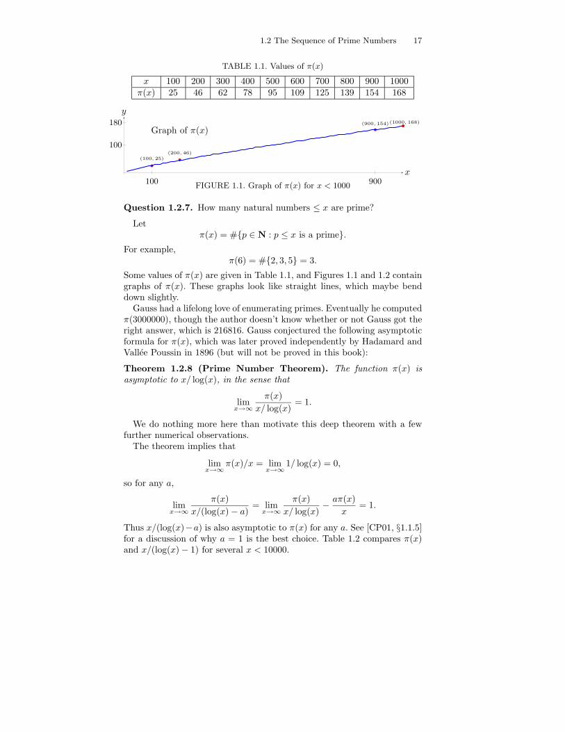
TABLE 1.1. Values of π(x)
x 100 200 300 400 500 600 700 800 900 1000π(x) 25 46 62 78 95 109 125 139 154 168
x
y
(100, 25)(200, 46)
(900, 154)(1000, 168)180
100
900100
Graph of π(x)
FIGURE 1.1. Graph of π(x) for x < 1000
Question 1.2.7. How many natural numbers ≤ x are prime?
Letπ(x) = #{p ∈ N : p ≤ x is a prime}.
For example,π(6) = #{2, 3, 5} = 3.
Some values of π(x) are given in Table 1.1, and Figures 1.1 and 1.2 containgraphs of π(x). These graphs look like straight lines, which maybe benddown slightly.
Gauss had a lifelong love of enumerating primes. Eventually he computedπ(3000000), though the author doesn’t know whether or not Gauss got theright answer, which is 216816. Gauss conjectured the following asymptoticformula for π(x), which was later proved independently by Hadamard andVallee Poussin in 1896 (but will not be proved in this book):
Theorem 1.2.8 (Prime Number Theorem). The function π(x) isasymptotic to x/ log(x), in the sense that
limx→∞
π(x)
x/ log(x)= 1.
We do nothing more here than motivate this deep theorem with a fewfurther numerical observations.
The theorem implies that
limx→∞
π(x)/x = limx→∞
1/ log(x) = 0,
so for any a,
limx→∞
π(x)
x/(log(x) − a)= lim
x→∞
π(x)
x/ log(x)− aπ(x)
x= 1.
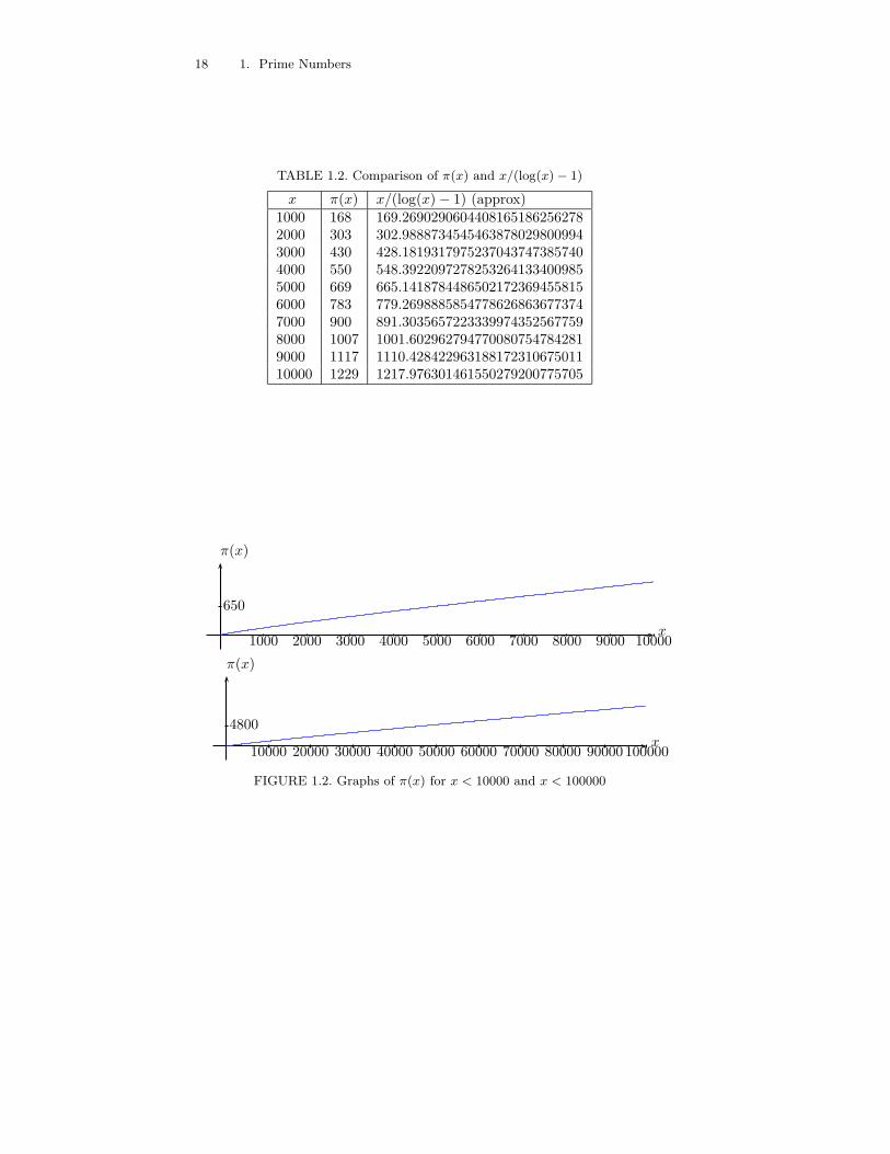
Thus x/(log(x)−a) is also asymptotic to π(x) for any a. See [CP01, §1.1.5]for a discussion of why a = 1 is the best choice. Table 1.2 compares π(x)and x/(log(x) − 1) for several x < 10000.
18 1. Prime Numbers
TABLE 1.2. Comparison of π(x) and x/(log(x)− 1)
x π(x) x/(log(x) − 1) (approx)
1000 168 169.26902906044081651862562782000 303 302.98887345454638780298009943000 430 428.18193179752370437473857404000 550 548.39220972782532641334009855000 669 665.14187844865021723694558156000 783 779.26988858547786268636773747000 900 891.30356572233399743525677598000 1007 1001.6029627947700807547842819000 1117 1110.42842296318817231067501110000 1229 1217.976301461550279200775705
x
π(x)
1000 2000 3000 4000 5000 6000 7000 8000 9000 10000
650
x
π(x)
10000 20000 30000 40000 50000 60000 70000 80000 90000100000
4800
FIGURE 1.2. Graphs of π(x) for x < 10000 and x < 100000
1.3 Exercises 19
As of 2004, the record for counting primes appears to be
π(4 · 1022) = 783964159847056303858.
The computation of π(4 · 1022) reportedly took ten months on a 350 MhzPentium II (see [GS02] for more details).
For the reader familiar with complex analysis, we mention a connectionbetween π(x) and the Riemann Hypothesis. The Riemann zeta functionζ(s) is a complex analytic function on C \ {1} that extends the functiondefined on a right half plane by
∑∞n=1 n−s. The Riemann Hypothesis is
the conjecture that the zeros in C of ζ(s) with positive real part lie on theline Re(s) = 1/2. This conjecture is one of the Clay Math Institute milliondollar millennium prize problems [Cla].
According to [CP01, §1.4.1], the Riemann Hypothesis is equivalent to theconjecture that
Li(x) =
∫ x
2
1
log(t)dt
is a “good” approximation to π(x), in the following precise sense:
Conjecture 1.2.9 (Equivalent to the Riemann Hypothesis).For all x ≥ 2.01,
|π(x) − Li(x)| ≤√
x log(x).
If x = 2, then π(2) = 1 and Li(2) = 0, but√
2 log(2) = 0.9802 . . ., so theinequality is not true for x ≥ 2, but 2.01 is big enough. We will do nothingmore to explain this conjecture, and settle for one numerical example.
Example 1.2.10. Let x = 4 · 1022. Then
π(x) = 783964159847056303858,
Li(x) = 783964159852157952242.7155276025801473 . . . ,
|π(x) − Li(x)| = 5101648384.71552760258014 . . . ,√
x log(x) = 10408633281397.77913344605 . . . ,
x/(log(x) − 1) = 783650443647303761503.5237113087392967 . . . .
One of the best popular article on the prime number theorem and theRiemann hypothesis is [Zag75].
1.3 Exercises
1.1 Compute the greatest common divisor gcd(455, 1235) by hand.
1.2 Use the Sieve of Eratosthenes to make a list of all primes up to 100.
1.3 Prove that there are infinitely many primes of the form 6x − 1.
1.4 Use Theorem 1.2.8 to deduce that limx→∞
π(x)
x= 0.

20 1. Prime Numbers
This is page 21Printer: Opaque this
2The Ring of Integers Modulo n
This chapter is about the ring Z/nZ of integers modulo n. First we discusswhen linear equations modulo n have a solution, then introduce the Euler ϕfunction and prove Fermat’s Little Theorem and Wilson’s theorem. Nextwe prove the Chinese Remainer Theorem, which addresses simultaneoussolubility of several linear equations modulo coprime moduli. With thesetheoretical foundations in place, in Section 2.3 we introduce algorithmsfor doing interesting computations modulo n, including computing largepowers quickly, and solving linear equations. We finish with a very briefdiscussion of finding prime numbers using arithmetic modulo n.
2.1 Congruences Modulo n
In this section we define the ring Z/nZ of integers modulo n, introducethe Euler ϕ-function, and relate it to the multiplicative order of certainelements of Z/nZ.
If a, b ∈ Z and n ∈ N, we say that a is congruent to b modulo n if n | a−b,and write a ≡ b (mod n). Let nZ = (n) be the ideal of Z generated by n.
Definition 2.1.1 (Integers Modulo n). The ring of integers modulo nis the quotient ring Z/nZ of equivalence classes of integers modulo n. It isequipped with its natural ring structure:
(a + nZ) + (b + nZ) = (a + b) + nZ
(a + nZ) · (b + nZ) = (a · b) + nZ.
22 2. The Ring of Integers Modulo n
Example 2.1.2. For example,
Z/3Z = {{. . . ,−3, 0, 3, . . .}, {. . . ,−2, 1, 4, . . .}, {. . . ,−1, 2, 5, . . .}}
We use the notation Z/nZ because Z/nZ is the quotient of the ring Zby the ideal nZ of multiples of n. Because Z/nZ is the quotient of a ringby an ideal, the ring structure on Z induces a ring structure on Z/nZ. Weoften let a or a (mod n) denote the equivalence class a + nZ of a. If p is aprime, then Z/pZ is a field (see Exercise 2.11).
We call the natural reduction map Z → Z/nZ, which sends a to a + nZ,reduction modulo n. We also say that a is a lift of a + nZ. Thus, e.g., 7 isa lift of 1 mod 3, since 7 + 3Z = 1 + 3Z.
We can use that arithmetic in Z/nZ is well defined is to derive tests fordivisibility by n (see Exercise 2.7).
Proposition 2.1.3. A number n ∈ Z is divisible by 3 if and only if thesum of the digits of n is divisible by 3.
Proof. Writen = a + 10b + 100c + · · · ,
where the digits of n are a, b, c, etc. Since 10 ≡ 1 (mod 3),
n = a + 10b + 100c + · · · ≡ a + b + c + · · · (mod 3),
from which the proposition follows.
2.1.1 Linear Equations Modulo n
In this section, we are concerned with how to decide whether or not a linearequation of the form ax ≡ b (mod n) has a solution modulo n. Algorithmsfor computing solutions to ax ≡ b (mod n) are the topic of Section 2.3.
First we prove a proposition that gives a criterion under which one cancancel a quantity from both sides of a congruence.
Proposition 2.1.4 (Cancellation). If gcd(c, n) = 1 and
ac ≡ bc (mod n),
then a ≡ b (mod n).
Proof. By definitionn | ac − bc = (a − b)c.
Since gcd(n, c) = 1, it follows from Theorem 1.1.5 that n | a − b, so
a ≡ b (mod n),
as claimed.
2.1 Congruences Modulo n 23
When a has a multiplicative inverse a′ in Z/nZ (i.e., aa′ ≡ 1 (mod n))then the equation ax ≡ b (mod n) has a unique solution x ≡ a′b (mod n)modulo n. Thus, it is of interest to determine the units in Z/nZ, i.e., theelements which have a multiplicative inverse.
We will use complete sets of residues to prove that the units in Z/nZare exactly the a ∈ Z/nZ such that gcd(a, n) = 1 for any lift a of a to Z(it doesn’t matter which lift).
Definition 2.1.5 (Complete Set of Residues). We call a subset R ⊂ Zof size n whose reductions modulo n are pairwise distinct a complete set ofresidues modulo n. In other words, a complete set of residues is a choice ofrepresentative for each equivalence class in Z/nZ.
For example,R = {0, 1, 2, . . . , n − 1}
is a complete set of residues modulo n. When n = 5, R = {0, 1,−1, 2,−2}is a complete set of residues.
Lemma 2.1.6. If R is a complete set of residues modulo n and a ∈ Z withgcd(a, n) = 1, then aR = {ax : x ∈ R} is also a complete set of residuesmodulo n.
Proof. If ax ≡ ax′ (mod n) with x, x′ ∈ R, then Proposition 2.1.4 impliesthat x ≡ x′ (mod n). Because R is a complete set of residues, this impliesthat x = x′. Thus the elements of aR have distinct reductions modulo n. Itfollows, since #aR = n, that aR is a complete set of residues modulo n.
Proposition 2.1.7 (Units). If gcd(a, n) = 1, then the equation ax ≡ b(mod n) has a solution, and that solution is unique modulo n.
Proof. Let R be a complete set of residues modulo n, so there is a uniqueelement of R that is congruent to b modulo n. By Lemma 2.1.6, aR is alsoa complete set of residues modulo n, so there is a unique element ax ∈ aRthat is congruent to b modulo n, and we have ax ≡ b (mod n).
Algebraically, this proposition asserts that if gcd(a, n) = 1, then the mapZ/nZ → Z/nZ given by left multiplication by a is a bijection.
Example 2.1.8. Consider the equation 2x ≡ 3 (mod 7), and the completeset R = {0, 1, 2, 3, 4, 5, 6} of coset representatives. We have
2R = {0, 2, 4, 6, 8 ≡ 1, 10 ≡ 3, 12 ≡ 5},
so 2 · 5 ≡ 3 (mod 7).
When gcd(a, n) 6= 1, then the equation ax ≡ b (mod n) may or maynot have a solution. For example, 2x ≡ 1 (mod 4) has no solution, but2x ≡ 2 (mod 4) does, and in fact it has more than one mod 4 (x = 1and x = 3). Generalizing Proposition 2.1.7, we obtain the following moregeneral criterion for solvability.

24 2. The Ring of Integers Modulo n
Proposition 2.1.9 (Solvability). The equation ax ≡ b (mod n) has asolution if and only if gcd(a, n) divides b.
Proof. Let g = gcd(a, n). If there is a solution x to the equation ax ≡ b(mod n), then n | (ax − b). Since g | n and g | a, it follows that g | b.
Conversely, suppose that g | b. Then n | (ax − b) if and only if
n
g|(
a
gx − b
g
)
.
Thus ax ≡ b (mod n) has a solution if and only if ag x ≡ b
g (mod ng ) has
a solution. Since gcd(a/g, n/g) = 1, Proposition 2.1.7 implies this latterequation does have a solution.
In Chapter 4 we will study quadratic reciprocity, which gives a nicecriterion for whether or not a quadratic equation modulo n has a solution.
2.1.2 Fermat’s Little Theorem
The group of units (Z/nZ)∗ of the ring Z/nZ will be of great interestto us. Each element of this group has an order, and Lagrange’s theoremfrom group theory implies that each element of (Z/nZ)∗ has order thatdivides the order of (Z/nZ)∗. In elementary number theory this fact goesby the monicker “Fermat’s Little Theorem”, and we reprove it from basicprinciples in this section.
Definition 2.1.10 (Order of an Element). Let n ∈ N and x ∈ Z andsuppose that gcd(x, n) = 1. The order of x modulo n is the smallest m ∈ Nsuch that
xm ≡ 1 (mod n).
To show that the definition makes sense, we verify that such an m exists.Consider x, x2, x3, . . . modulo n. There are only finitely many residue classesmodulo n, so we must eventually find two integers i, j with i < j such that
xj ≡ xi (mod n).
Since gcd(x, n) = 1, Proposition 2.1.4 implies that we can cancel x’s andconclude that
xj−i ≡ 1 (mod n).
Definition 2.1.11 (Euler’s phi-function). For n ∈ N, let
ϕ(n) = #{a ∈ N : a ≤ n and gcd(a, n) = 1}.
2.1 Congruences Modulo n 25
For example,
ϕ(1) = #{1} = 1,
ϕ(2) = #{1} = 1,
ϕ(5) = #{1, 2, 3, 4} = 4,
ϕ(12) = #{1, 5, 7, 11} = 4.
Also, if p is any prime number then
ϕ(p) = #{1, 2, . . . , p − 1} = p − 1.
In Section 2.2.1, we will prove that ϕ is a multiplicative function. This willyield an easy way to compute ϕ(n) in terms of the prime factorization of n.
Theorem 2.1.12 (Fermat’s Little Theorem). If gcd(x, n) = 1, then
xϕ(n) ≡ 1 (mod n).
Proof. As mentioned above, Fermat’s Little Theorem has the followinggroup-theoretic interpretation. The set of units in Z/nZ is a group
(Z/nZ)∗ = {a ∈ Z/nZ : gcd(a, n) = 1}.
which has order ϕ(n). The theorem then asserts that the order of an elementof (Z/nZ)∗ divides the order ϕ(n) of (Z/nZ)∗. This is a special case of themore general fact (Lagrange’s theorem) that if G is a finite group andg ∈ G, then the order of g divides the cardinality of G.
We now give an elementary proof of the theorem. Let
P = {a : 1 ≤ a ≤ n and gcd(a, n) = 1}.
In the same way that we proved Lemma 2.1.6, we see that the reductionsmodulo n of the elements of xP are the same as the reductions of theelements of P . Thus
∏
a∈P
(xa) ≡∏
a∈P
a (mod n),
since the products are over the same numbers modulo n. Now cancel thea’s on both sides to get
x#P ≡ 1 (mod n),
as claimed.
26 2. The Ring of Integers Modulo n
2.1.3 Wilson’s Theorem
The following characterization of prime numbers, from the 1770s, is called“Wilson’s Theorem”, though it was first proved by Lagrange.
Proposition 2.1.13 (Wilson’s Theorem). An integer p > 1 is prime ifand only if (p − 1)! ≡ −1 (mod p).
For example, if p = 3, then (p − 1)! = 2 ≡ −1 (mod 3). If p = 17, then
(p − 1)! = 20922789888000 ≡ −1 (mod 17).
But if p = 15, then
(p − 1)! = 87178291200 ≡ 0 (mod 15),
so 15 is composite. Thus Wilson’s theorem could be viewed as a primalitytest, though, from a computational point of view, it is probably the leastefficient primality test since computing (n − 1)! takes so many steps.
Proof. The statement is clear when p = 2, so henceforth we assume thatp > 2. We first assume that p is prime and prove that (p − 1)! ≡ −1(mod p). If a ∈ {1, 2, . . . , p − 1} then the equation
ax ≡ 1 (mod p)
has a unique solution a′ ∈ {1, 2, . . . , p− 1}. If a = a′, then a2 ≡ 1 (mod p),so p | a2−1 = (a−1)(a+1), so p | (a−1) or p | (a+1), so a ∈ {1, p−1}. Wecan thus pair off the elements of {2, 3, . . . , p − 2}, each with their inverse.Thus
2 · 3 · · · · · (p − 2) ≡ 1 (mod p).
Multiplying both sides by p − 1 proves that (p − 1)! ≡ −1 (mod p).Next we assume that (p − 1)! ≡ −1 (mod p) and prove that p must be
prime. Suppose not, so that p ≥ 4 is a composite number. Let ℓ be a primedivisor of p. Then ℓ < p, so ℓ | (p − 1)!. Also, by assumption,
ℓ | p | ((p − 1)! + 1).
This is a contradiction, because a prime can not divide a number a andalso divide a + 1, since it would then have to divide (a + 1) − a = 1.
Example 2.1.14. We illustrate the key step in the above proof in the casep = 17. We have
2·3 · · · 15 = (2·9)·(3·6)·(4·13)·(5·7)·(8·15)·(10·12)·(14·11) ≡ 1 (mod 17),
where we have paired up the numbers a, b for which ab ≡ 1 (mod 17).
2.2 The Chinese Remainder Theorem 27
2.2 The Chinese Remainder Theorem
In this section we prove the Chinese Remainder Theorem, which gives con-ditions under which a system of linear equations is guaranteed to have asolution. In the 4th century a Chinese mathematician asked the following:
Question 2.2.1. There is a quantity whose number is unknown. Repeat-edly divided by 3, the remainder is 2; by 5 the remainder is 3; and by 7 theremainder is 2. What is the quantity?
In modern notation, Question 2.2.1 asks us to find a positive integersolution to the following system of three equations:
x ≡ 2 (mod 3)
x ≡ 3 (mod 5)
x ≡ 2 (mod 7)
The Chinese Remainder Theorem asserts that a solution exists, and theproof gives a method to find one. (See Section 2.3 for the necessary algo-rithms.)
Theorem 2.2.2 (Chinese Remainder Theorem). Let a, b ∈ Z andn,m ∈ N such that gcd(n,m) = 1. Then there exists x ∈ Z such that
x ≡ a (mod m),
x ≡ b (mod n).
Moreover x is unique modulo mn.
Proof. If we can solve for t in the equation
a + tm ≡ b (mod n),
then x = a + tm will satisfy both congruences. To see that we can solve,subtract a from both sides and use Proposition 2.1.7 together with ourassumption that gcd(n,m) = 1 to see that there is a solution.
For uniqueness, suppose that x and y solve both congruences. Then z =x−y satisfies z ≡ 0 (mod m) and z ≡ 0 (mod n), so m | z and n | z. Sincegcd(n,m) = 1, it follows that nm | z, so x ≡ y (mod nm).
Algorithm 2.2.3 (Chinese Remainder Theorem). Given coprime in-tegers m and n and integers a and b, this algorithm find an integer x suchthat x ≡ a (mod m) and x ≡ b (mod n).
1. [Extended GCD] Use Algorithm 2.3.3 below to find integers c, d suchthat cm + dn = 1.
2. [Answer] Output x = a + (b − a)cm and terminate.
28 2. The Ring of Integers Modulo n
Proof. Since c ∈ Z, we have x ≡ a (mod m), and using that cm + dn = 1,we have a + (b − a)cm ≡ a + (b − a) ≡ b (mod n).
Now we can answer Question 2.2.1. First, we use Theorem 2.2.2 to finda solution to the pair of equations
x ≡ 2 (mod 3),
x ≡ 3 (mod 5).
Set a = 2, b = 3, m = 3, n = 5. Step 1 is to find a solution to t · 3 ≡ 3 − 2(mod 5). A solution is t = 2. Then x = a + tm = 2 + 2 · 3 = 8. Since any x′
with x′ ≡ x (mod 15) is also a solution to those two equations, we cansolve all three equations by finding a solution to the pair of equations
x ≡ 8 (mod 15)
x ≡ 2 (mod 7).
Again, we find a solution to t · 15 ≡ 2 − 8 (mod 7). A solution is t = 1, so
x = a + tm = 8 + 15 = 23.
Note that there are other solutions. Any x′ ≡ x (mod 3 · 5 · 7) is also asolution; e.g., 23 + 3 · 5 · 7 = 128.
2.2.1 Multiplicative Functions
Definition 2.2.4 (Multiplicative Function). A function f : N → Z ismultiplicative if, whenever m,n ∈ N and gcd(m,n) = 1, we have
f(mn) = f(m) · f(n).
Recall from Definition 2.1.11 that the Euler ϕ-function is
ϕ(n) = #{a : 1 ≤ a ≤ n and gcd(a, n) = 1}.Lemma 2.2.5. Suppose that m,n ∈ N and gcd(m,n) = 1. Then the map
ψ : (Z/mnZ)∗ → (Z/mZ)∗ × (Z/nZ)∗. (2.2.1)
defined byψ(c) = (c mod m, c mod n)
is a bijection.
Proof. We first show that ψ is injective. If ψ(c) = ψ(c′), then m | c−c′ andn | c − c′, so nm | c − c′ because gcd(n,m) = 1. Thus c = c′ as elements of(Z/mnZ)∗.
Next we show that ψ is surjective. Given a and b with gcd(a,m) = 1and gcd(b, n) = 1, Theorem 2.2.2 implies that there exists c with c ≡ a(mod m) and c ≡ b (mod n). We may assume that 1 ≤ c ≤ nm, andsince gcd(a,m) = 1 and gcd(b, n) = 1, we must have gcd(c, nm) = 1. Thusψ(c) = (a, b).
2.3 Quickly Computing Inverses and Huge Powers 29
Proposition 2.2.6 (Multiplicativity of ϕ). The function ϕ is multi-plicative.
Proof. The map ψ of Lemma 2.2.5 is a bijection, so the set on the left in(2.2.1) has the same size as the product set on the right in (2.2.1). Thus
ϕ(mn) = ϕ(m) · ϕ(n).
The proposition is helpful in computing ϕ(n), at least if we assume we cancompute the factorization of n (see Section 3.3.1 for a connection betweenfactoring n and computing ϕ(n)). For example,
ϕ(12) = ϕ(22) · ϕ(3) = 2 · 2 = 4.
Also, for n ≥ 1, we have
ϕ(pn) = pn − pn
p= pn − pn−1 = pn−1(p − 1), (2.2.2)
since ϕ(pn) is the number of numbers less than pn minus the number ofthose that are divisible by p. Thus, e.g.,
ϕ(389 · 112) = 388 · (112 − 11) = 388 · 110 = 42680.
2.3 Quickly Computing Inverses and Huge Powers
This section is about how to solve the equation ax ≡ 1 (mod n) whenwe know it has a solution, and how to efficiently compute am (mod n).We also discuss a simple probabilistic primality test that relies on ourability to compute am (mod n) quickly. All three of these algorithms areof fundamental importance to the cryptography algorithms of Chapter 3.
2.3.1 How to Solve ax ≡ 1 (mod n)
Suppose a, n ∈ N with gcd(a, n) = 1. Then by Proposition 2.1.7 the equa-tion ax ≡ 1 (mod n) has a unique solution. How can we find it?
Proposition 2.3.1 (Extended Euclidean representation). Supposea, b ∈ Z and let g = gcd(a, b). Then there exists x, y ∈ Z such that
ax + by = g.
Remark 2.3.2. If e = cg is a multiple of g, then cax + cby = cg = e, soe = (cx)a + (cy)b can also be written in terms of a and b.
30 2. The Ring of Integers Modulo n
Proof of Proposition 2.3.1. Let g = gcd(a, b). Then gcd(a/d, b/d) = 1, soby Proposition 2.1.9 the equation
a
g· x ≡ 1
(
modb
g
)
(2.3.1)
has a solution x ∈ Z. Multiplying (2.3.1) through by g yields ax ≡ g(mod b), so there exists y such that b · (−y) = ax − g. Then ax + by = g,as required.
Given a, b and g = gcd(a, b), our proof of Proposition 2.3.1 gives a way toexplicitly find x, y such that ax+by = g, assuming one knows an algorithmto solve linear equations modulo n. Since we do not know such an algorithm,we now discuss a way to explicitly find x and y. This algorithm will in factenable us to solve linear equations modulo n—to solve ax ≡ 1 (mod n)when gcd(a, n) = 1, use the algorithm below to find x and y such thatax + ny = 1. Then ax ≡ 1 (mod n).
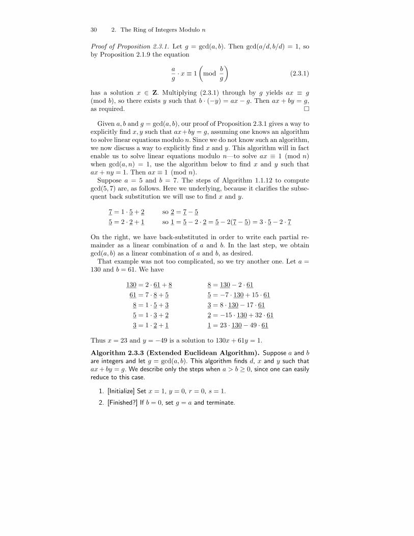
Suppose a = 5 and b = 7. The steps of Algorithm 1.1.12 to computegcd(5, 7) are, as follows. Here we underlying, because it clarifies the subse-quent back substitution we will use to find x and y.
7 = 1 · 5 + 2 so 2 = 7 − 5
5 = 2 · 2 + 1 so 1 = 5 − 2 · 2 = 5 − 2(7 − 5) = 3 · 5 − 2 · 7
On the right, we have back-substituted in order to write each partial re-mainder as a linear combination of a and b. In the last step, we obtaingcd(a, b) as a linear combination of a and b, as desired.
That example was not too complicated, so we try another one. Let a =130 and b = 61. We have
130 = 2 · 61 + 8 8 = 130 − 2 · 61
61 = 7 · 8 + 5 5 = −7 · 130 + 15 · 61
8 = 1 · 5 + 3 3 = 8 · 130 − 17 · 61
5 = 1 · 3 + 2 2 = −15 · 130 + 32 · 61
3 = 1 · 2 + 1 1 = 23 · 130 − 49 · 61
Thus x = 23 and y = −49 is a solution to 130x + 61y = 1.
Algorithm 2.3.3 (Extended Euclidean Algorithm). Suppose a and bare integers and let g = gcd(a, b). This algorithm finds d, x and y such thatax + by = g. We describe only the steps when a > b ≥ 0, since one can easilyreduce to this case.
1. [Initialize] Set x = 1, y = 0, r = 0, s = 1.
2. [Finished?] If b = 0, set g = a and terminate.
2.3 Quickly Computing Inverses and Huge Powers 31
3. [Quotient and Remainder] Use Algorithm 1.1.11 to write a = qb+c with0 ≤ c < b.
4. [Shift] Set (a, b, r, s, x, y) = (b, c, x − qr, y − qs, r, s) and go to step 2.
Proof. This algorithm is the same as Algorithm 1.1.12, except that we keeptrack of extra variables x, y, r, s, so it terminates and when it terminatesd = gcd(a, b). We omit the rest of the inductive proof that the algorithmis correct, and instead refer the reader to [Knu97, §1.2.1] which contains adetailed proof in the context of a discussion of how one writes mathematicalproofs.
Algorithm 2.3.4 (Inverse Modulo n). Suppose a and n are integers andgcd(a, n) = 1. This algorithm finds an x such that ax ≡ 1 (mod n).
1. [Compute Extended GCD] Use Algorithm 2.3.3 to compute integers x, ysuch that ax + ny = gcd(a, n) = 1.
2. [Finished] Output x.
Proof. Reduce ax+ny = 1 modulo n to see that x satisfies ax ≡ 1 (mod n).
See Section 7.2.1 for implementations of Algorithms 2.3.3 and 2.3.4.
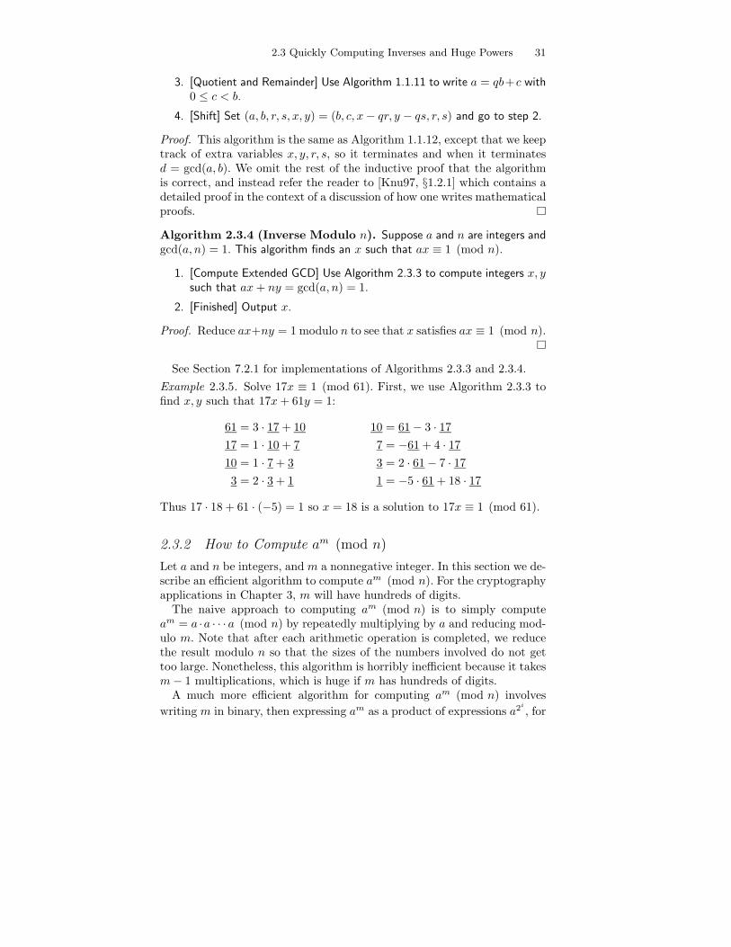
Example 2.3.5. Solve 17x ≡ 1 (mod 61). First, we use Algorithm 2.3.3 tofind x, y such that 17x + 61y = 1:
61 = 3 · 17 + 10 10 = 61 − 3 · 17
17 = 1 · 10 + 7 7 = −61 + 4 · 17
10 = 1 · 7 + 3 3 = 2 · 61 − 7 · 17
3 = 2 · 3 + 1 1 = −5 · 61 + 18 · 17
Thus 17 · 18 + 61 · (−5) = 1 so x = 18 is a solution to 17x ≡ 1 (mod 61).
2.3.2 How to Compute am (mod n)
Let a and n be integers, and m a nonnegative integer. In this section we de-scribe an efficient algorithm to compute am (mod n). For the cryptographyapplications in Chapter 3, m will have hundreds of digits.
The naive approach to computing am (mod n) is to simply computeam = a ·a · · · a (mod n) by repeatedly multiplying by a and reducing mod-ulo m. Note that after each arithmetic operation is completed, we reducethe result modulo n so that the sizes of the numbers involved do not gettoo large. Nonetheless, this algorithm is horribly inefficient because it takesm − 1 multiplications, which is huge if m has hundreds of digits.
A much more efficient algorithm for computing am (mod n) involves
writing m in binary, then expressing am as a product of expressions a2i
, for
32 2. The Ring of Integers Modulo n
various i. These latter expressions can be computed by repeatedly squaringa2i
. This more clever algorithm is not “simpler”, but it is vastly moreefficient since the number of operations needed grows with the number ofbinary digits of m, whereas with the naive algorithm above the number ofoperations is m − 1.
Algorithm 2.3.6 (Write a number in binary). Let m be a nonnegativeinteger. This algorithm writes m in binary, so it finds εi ∈ {0, 1} such thatm =
∑ri=0 εi2
i with each εi ∈ {0, 1}.1. [Initialize] Set i = 0.
2. [Finished?] If m = 0, terminate.
3. [Digit] If m is odd, set εi = 1, otherwise εi = 0. Increment i.
4. [Divide by 2] Set m =⌊
m2
⌋
, the greatest integer ≤ m/2. Goto step 2.
Algorithm 2.3.7 (Compute Power). Let a and n be integers and m anonnegative integer. This algorithm computes am modulo n.
1. [Write in Binary] Write m in binary using Algorithm 2.3.6, so am =∏
εi=1 a2i
(mod n).
2. [Compute Powers] Compute a, a2, a22
= (a2)2, a23
= (a22
)2, etc., upto a2r
, where r + 1 is the number of binary digits of m.
3. [Multiply Powers] Multiply together the a2i
such that εi = 1, alwaysworking modulo n.
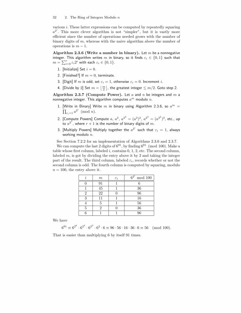
See Section 7.2.2 for an implementation of Algorithms 2.3.6 and 2.3.7.We can compute the last 2 digits of 691, by finding 691 (mod 100). Make a
table whose first column, labeled i, contains 0, 1, 2, etc. The second column,labeled m, is got by dividing the entry above it by 2 and taking the integerpart of the result. The third column, labeled εi, records whether or not thesecond column is odd. The fourth column is computed by squaring, modulon = 100, the entry above it.
i m εi 62i
mod 100
0 91 1 6
1 45 1 36
2 22 0 963 11 1 16
4 5 1 56
5 2 0 366 1 1 96
We have
691 ≡ 626 · 624 · 623 · 62 · 6 ≡ 96 · 56 · 16 · 36 · 6 ≡ 56 (mod 100).
That is easier than multiplying 6 by itself 91 times.
2.4 Finding Primes 33
Remark 2.3.8. Alternatively, we could simplify the computation using The-orem 2.1.12. By that theorem, 6ϕ(100) ≡ 1 (mod 100), so since ϕ(100) =ϕ(22 · 52) = (22 − 2) · (52 − 5) = 40, we have 691 ≡ 611 (mod 100).
2.4 Finding Primes
Theorem 2.4.1 (Pseudoprimality). An integer p > 1 is prime if andonly if for every a 6≡ 0 (mod p),
ap−1 ≡ 1 (mod p).
Proof. If p is prime, then the statement follows from Proposition 2.1.13.If p is composite, then there is a divisor a of p with a 6= 1, p. If ap−1 ≡ 1(mod p), then p | ap−1 − 1. Since a | p, we have a | ap−1 − 1 hence a | 1, acontradiction.
Suppose n ∈ N. Using this theorem and Algorithm 2.3.7, we can eitherquickly prove that n is not prime, or convince ourselves that n is likelyprime (but not quickly prove that n is prime). For example, if 2n−1 6≡ 1(mod n), then we have proved that n is not prime. On the other hand,if an−1 ≡ 1 (mod n) for a few a, it “seems likely” that n is prime, andwe loosely refer to such a number that seems prime for several bases as apseudoprime.
There are composite numbers n (called Carmichael numbers) with theamazing property that an−1 ≡ 1 (mod n) for all a with gcd(a, n) = 1. Thefirst Carmichael number is 561, and it is a theorem that there are infinitelymany such numbers ([AGP94]).
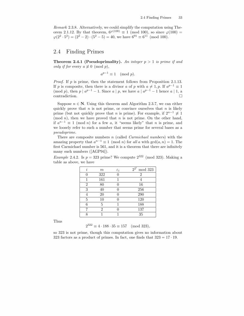
Example 2.4.2. Is p = 323 prime? We compute 2322 (mod 323). Making atable as above, we have
i m εi 22i
mod 323
0 322 0 2
1 161 1 42 80 0 16
3 40 0 256
4 20 0 2905 10 0 120
6 5 1 188
7 2 0 137
8 1 1 35
Thus2322 ≡ 4 · 188 · 35 ≡ 157 (mod 323),
so 323 is not prime, though this computation gives no information about323 factors as a product of primes. In fact, one finds that 323 = 17 · 19.
34 2. The Ring of Integers Modulo n
It’s possible to easily prove that a large number is composite, but theproof does not easily yield a factorization. For example if
n = 95468093486093450983409583409850934850938459083,
then 2n−1 6≡ 1 (mod n), so n is composite.Another practical primality test is the Miller-Rabin test, which has the
property that each time it is run on a number n it either correctly assertsthat the number is definitely not prime, or that it is probably prime, andthe probability of correctness goes up with each successive call. For a pre-cise statement and implementation of Miller-Rabin, along with proof ofcorrectness, see Section 7.2.4. If Miller-Rabin is called m times on n andin each case claims that n is probably prime, then one can in a precisesense bound the probability that n is composite in terms of m. For animplementation of Miller-Rabin, see Listing 7.2.9 in Chapter 7.
Until recently it was an open problem to give an algorithm (with proof)that decides whether or not any integer is prime in time bounded by a poly-nomial in the number of digits of the integer. Agrawal, Kayal, and Saxenarecently found the first polynomial-time primality test (see [AKS02]). Wewill not discuss their algorithm further, because for our applications tocryptography Miller-Rabin or pseudoprimality tests will be sufficient.
2.5 The Structure of (Z/pZ)∗
This section is about the structure of the group (Z/pZ)∗ of units moduloa prime number p. The main result is that this group is always cyclic. Wewill use this result later in Chapter 4 in our proof of quadratic reciprocity.
Definition 2.5.1 (Primitive root). A primitive root modulo an integer nis an element of (Z/nZ)∗ of order ϕ(n).
We will prove that there is a primitive root modulo every prime p. Sincethe unit group (Z/pZ)∗ has order p−1, this implies that (Z/pZ)∗ is a cyclicgroup, a fact this will be extremely useful, since it completely determinesthe structure of (Z/pZ)∗ as an abelian group.
If n is an odd prime power, then there is a primitive root modulo n (seeExercise 2.25), but there is no primitive root modulo the prime power 23,and hence none mod 2n for n ≥ 3 (see Exercise 2.24).
Section 2.5.1 is the key input to our proof that (Z/pZ)∗ is cyclic; herewe show that for every divisor d of p − 1 there are exactly d elements of(Z/pZ)∗ whose order divides d. We then use this result in Section 2.5.2 toproduce an element of (Z/pZ)∗ of order qr when qr is a prime power thatexactly divides p− 1 (i.e., qr divides p− 1, but qr+1 does not divide p− 1),and multiply together these elements to obtain an element of (Z/pZ)∗ oforder p − 1.
2.5 The Structure of (Z/pZ)∗ 35
2.5.1 Polynomials over Z/pZ
The polynomials x2 − 1 has four roots in Z/8Z, namely 1, 3, 5, and 7.In contrast, the following proposition shows that a polynomial of degree dover a field, such as Z/pZ, can have at most d roots.
Proposition 2.5.2 (Root Bound). Let f ∈ k[x] be a nonzero polynomialover a field k. Then there are at most deg(f) elements α ∈ k such thatf(α) = 0.
Proof. We prove the proposition by induction on deg(f). The cases in whichdeg(f) ≤ 1 are clear. Write f = anxn + · · · a1x + a0. If f(α) = 0 then
f(x) = f(x) − f(α)
= an(xn − αn) + · · · a1(x − α) + a0(1 − 1)
= (x − α)(an(xn−1 + · · · + αn−1) + · · · + a2(x + α) + a1)
= (x − α)g(x),
for some polynomial g(x) ∈ k[x]. Next suppose that f(β) = 0 with β 6= α.Then (β − α)g(β) = 0, so, since β − α 6= 0, we have g(β) = 0. By ourinductive hypothesis, g has at most n− 1 roots, so there are at most n− 1possibilities for β. It follows that f has at most n roots.
Proposition 2.5.3. Let p be a prime number and let d be a divisor ofp − 1. Then f = xd − 1 ∈ (Z/pZ)[x] has exactly d roots in Z/pZ.
Proof. Let e = (p − 1)/d. We have
xp−1 − 1 = (xd)e − 1
= (xd − 1)((xd)e−1 + (xd)e−2 + · · · + 1)
= (xd − 1)g(x),
where g ∈ (Z/pZ)[x] and deg(g) = de − d = p − 1 − d. Theorem 2.1.12implies that xp−1 − 1 has exactly p− 1 roots in Z/pZ, since every nonzeroelement of Z/pZ is a root! By Proposition 2.5.2, g has at most p − 1 − droots and xd − 1 has at most d roots. Since a root of (xd − 1)g(x) is a rootof either xd − 1 or g(x) and xp−1 − 1 has p − 1 roots, g must have exactlyp − 1 − d roots and xd − 1 must have exactly d roots, as claimed.
We pause to reemphasize that the analogue of Proposition 2.5.3 is falsewhen p is replaced by a composite integer n, since a root mod n of aproduct of two polynomials need not be a root of either factor. For example,f = x2 − 1 ∈ Z/15Z[x] has the four roots 1, 4, 11, and 14.
36 2. The Ring of Integers Modulo n
2.5.2 Existence of Primitive Roots
Recall from Section 2.1.2 that the order of an element x in a finite groupis the smallest m ≥ 1 such that xm = 1. In this section, we prove that(Z/pZ)∗ is cyclic by using the results of Section 2.5.1 to produce an elementof (Z/pZ)∗ of order d for each prime power divisor d of p− 1, and then wemultiply these together to obtain an element of order p − 1.
We will use the following lemma to assemble elements of each orderdividing p − 1 to produce an element of order p − 1.
Lemma 2.5.4. Suppose a, b ∈ (Z/nZ)∗ have orders r and s, respectively,and that gcd(r, s) = 1. Then ab has order rs.
Proof. This is a general fact about commuting elements of any group; ourproof only uses that ab = ba and nothing special about (Z/nZ)∗. Since
(ab)rs = arsbrs = 1,
the order of ab is a divisor of rs. Write this divisor as r1s1 where r1 | r ands1 | s. Raise both sides of the equation
ar1s1br1s1 = (ab)r1s1 = 1.
to the power r2 = r/r1 to obtain
ar1r2s1br1r2s1 = 1.
Since ar1r2s1 = (ar1r2)s1 = 1, we have
br1r2s1 = 1,
so s | r1r2s1. Since gcd(s, r1r2) = gcd(s, r) = 1, it follows that s = s1.Similarly r = r1, so the order of ab is rs.
Theorem 2.5.5 (Primitive Roots). There is a primitive root moduloany prime p. In particular, the group (Z/pZ)∗ is cyclic.
Proof. The theorem is true if p = 2, since 1 is a primitive root, so we mayassume p > 2. Write p − 1 as a product of distinct prime powers qni
i :
p − 1 = qn11 qn2
2 · · · qnr
r .
By Proposition 2.5.3, the polynomial xqnii − 1 has exactly qni
i roots, and
the polynomial xqni−1
i − 1 has exactly qni−1i roots. There are qni
i − qni−1i =
qni−1i (qi − 1) elements a ∈ Z/pZ such that aq
nii = 1 but aq
ni−1
i 6= 1; eachof these elements has order qni
i . Thus for each i = 1, . . . , r, we can choosean ai of order qni
i . Then, using Lemma 2.5.4 repeatedly, we see that
a = a1a2 · · · ar
has order qn11 · · · qnr
r = p − 1, so a is a primitive root modulo p.
2.5 The Structure of (Z/pZ)∗ 37
Example 2.5.6. We illustrate the proof of Theorem 2.5.5 when p = 13. Wehave
p − 1 = 12 = 22 · 3.
The polynomial x4 − 1 has roots {1, 5, 8, 12} and x2 − 1 has roots {1, 12},so we may take a1 = 5. The polynomial x3 − 1 has roots {1, 3, 9}, and weset a2 = 3. Then a = 5 · 3 = 15 ≡ 2 is a primitive root. To verify this, notethat the successive powers of 2 (mod 13) are
2, 4, 8, 3, 6, 12, 11, 9, 5, 10, 7, 1.
Example 2.5.7. Theorem 2.5.5 is false if, e.g., p is replaced by a power of 2bigger than 4. For example, the four elements of (Z/8Z)∗ each have orderdividing 2, but ϕ(8) = 4.
Theorem 2.5.8 (Primitive Roots mod pn). Let pn be a power of anodd prime. Then there is a primitive root modulo pn.
The proof is left as Exercise 2.25.
Proposition 2.5.9 (Number of primitive roots). If there is a primitiveroot modulo n, then there are exactly ϕ(ϕ(n)) primitive roots modulo n.
Proof. The primitive roots modulo n are the generators of (Z/nZ)∗, whichby assumption is cyclic of order ϕ(n). Thus they are in bijection with thegenerators of any cyclic group of order ϕ(n). In particular, the number ofprimitive roots modulo n is the same as the number of elements of Z/ϕ(n)Zwith additive order ϕ(n). An element of Z/ϕ(n)Z has additive order ϕ(n)if and only if it is coprime to ϕ(n). There are ϕ(ϕ(n)) such elements, asclaimed.
Example 2.5.10. For example, there are ϕ(ϕ(17)) = ϕ(16) = 24 − 23 =8 primitive roots mod 17, namely 3, 5, 6, 7, 10, 11, 12, 14. The ϕ(ϕ(9)) =ϕ(6) = 2 primitive roots modulo 9 are 2 and 5. There are no primitiveroots modulo 8, even though ϕ(ϕ(8)) = ϕ(4) = 2 > 0.
2.5.3 Artin’s Conjecture
Conjecture 2.5.11 (Emil Artin). Suppose a ∈ Z is not −1 or a perfectsquare. Then there are infinitely many primes p such that a is a primitiveroot modulo p.
There is no single integer a such that Artin’s conjecture is known tobe true. For any given a, Pieter [Mor93] proved that there are infinitelymany p such that the order of a is divisible by the largest prime factorof p − 1. Hooley [Hoo67] proved that something called the GeneralizedRiemann Hypothesis implies Conjecture 2.5.11.
38 2. The Ring of Integers Modulo n
Remark 2.5.12. Artin conjectured more precisely that if N(x, a) is thenumber of primes p ≤ x such that a is a primitive root modulo p, thenN(x, a) is asymptotic to C(a)π(x), where C(a) is a positive constant thatdepends only on a and π(x) is the number of primes up to x.
2.5.4 Computing Primitive Roots
Theorem 2.5.5 does not suggest an efficient algorithm for finding primitiveroots. To actually find a primitive root mod p in practice, we try a = 2,then a = 3, etc., until we find an a that has order p − 1. Computing theorder of an element of (Z/pZ)∗ requires factoring p − 1, which we do notknow how to do quickly in general, so finding a primitive root modulo pfor large p seems to be a difficult problem.
See Section 7.2.3 for an implementation of this algorithm for finding aprimitive root.
Algorithm 2.5.13 (Primitive Root). Given a prime p this algorithmcomputes the smallest positive integer a that generates (Z/pZ)∗.
1. [p = 2?] If p = 2 output 1 and terminate. Otherwise set a = 2.
2. [Prime Divisors] Compute the prime divisors p1, . . . , pr of p − 1 (seeSection 7.1.3).
3. [Generator?] If for every pi, we have a(p−1)/pi 6≡ 1 (mod p), then a is agenerator of (Z/pZ)∗, so output a and terminate.
4. [Try next] Set a = a + 1 and go to step 3.
Proof. Let a ∈ (Z/pZ)∗. The order of a is a divisor d of the order p − 1 ofthe group (Z/pZ)∗. Write d = (p− 1)/n, for some divisor n of p− 1. If a isnot a generator of (Z/pZ)∗, then since n | (p − 1), there is a prime divisorpi of p − 1 such that pi | n. Then
a(p−1)/pi = (a(p−1)/n)n/pi ≡ 1 (mod p).
Conversely, if a is a generator, then a(p−1)/pi 6≡ 1 (mod p) for any pi. Thusthe algorithm terminates with step 3 if and only if the a under considerationis a primitive root. By Theorem 2.5.5 there is at least one primitive root,so the algorithm terminates.
We implement Algorithm 2.5.13 in Section 7.2.3.
2.6 Exercises
2.1 Compute the following gcd’s using Algorithm 1.1.12:
gcd(15, 35), gcd(247, 299), gcd(51, 897), gcd(136, 304)
2.6 Exercises 39
2.2 Use Algorithm 2.3.3 to find x, y ∈ Z such that 2261x + 1275y = 17.
2.3 Prove that if a and b are integers and p is a prime, then (a + b)p ≡ap + bp (mod p). You may assume that the binomial coefficient
p!
r!(p − r)!
is an integer.
2.4 (a) Prove that if x, y is a solution to ax+ by = d, then for all c ∈ Z,
x′ = x + c · b
d, y′ = y − c · a
d(2.6.1)
is also a solution to ax + by = d.
(b) Find two distinct solutions to 2261x + 1275y = 17.
(c) Prove that all solutions are of the form (2.6.1) for some c.
2.5 Let f(x) = x2 + ax + b ∈ Z[x] be a quadratic polynomial with inte-ger coefficients and positive leading coefficients, e.g., f(x) = x2 +x + 6. Formulate a conjecture about when the set {f(n) : n ∈Z and f(n) is prime} is infinite. Give numerical evidence that sup-ports your conjecture.
2.6 Find four complete sets of residues modulo 7, where the ith set sat-isfies the ith condition: (1) nonnegative, (2) odd, (3) even, (4) prime.
2.7 Find rules in the spirit of Proposition 2.1.3 for divisibility of an integerby 5, 9, and 11, and prove each of these rules using arithmetic moduloa suitable n.
2.8 (*) The following problem is from the 1998 Putnam Competition.Define a sequence of decimal integers an as follows: a1 = 0, a2 =1, and an+2 is obtained by writing the digits of an+1 immediatelyfollowed by those of an. For example, a3 = 10, a4 = 101, and a5 =10110. Determine the n such that an a multiple of 11, as follows:
(a) Find the smallest integer n > 1 such that an is divisible by 11.
(b) Prove that an is divisible by 11 if and only if n ≡ 1 (mod 6).
2.9 Find an integer x such that 37x ≡ 1 (mod 101).
2.10 What is the order of 2 modulo 17?
2.11 Let p be a prime. Prove that Z/pZ is a field.
2.12 Find an x ∈ Z such that x ≡ −4 (mod 17) and x ≡ 3 (mod 23).
40 2. The Ring of Integers Modulo n
2.13 Prove that if n > 4 is composite then
(n − 1)! ≡ 0 (mod n).
2.14 For what values of n is ϕ(n) odd?
2.15 (a) Prove that ϕ is multiplicative as follows. Suppose m,n are pos-itive integers and gcd(m,n) = 1. Show that the natural mapψ : Z/mnZ → Z/mZ × Z/nZ is an injective homomorphism ofrings, hence bijective by counting, then look at unit groups.
(b) Prove conversely that if gcd(m,n) > 1 then the natural mapψ : Z/mnZ → Z/mZ × Z/nZ is not an isomorphism.
2.16 Seven competitive math students try to share a huge hoard of stolenmath books equally between themselves. Unfortunately, six books areleft over, and in the fight over them, one math student is expelled.The remaining six math students, still unable to share the math booksequally since two are left over, again fight, and another is expelled.When the remaining five share the books, one book is left over, andit is only after yet another math student is expelled that an equalsharing is possible. What is the minimum number of books whichallow this to happen?
2.17 Show that if p is a positive integer such that both p and p2 + 2 areprime, then p = 3.
2.18 Let ϕ : N → N be the Euler ϕ function.
(a) Find all natural numbers n such that ϕ(n) = 1.
(b) Do there exist natural numbers m and n such that ϕ(mn) 6=ϕ(m) · ϕ(n)?
2.19 Find a formula for ϕ(n) directly in terms of the prime factorizationof n.
2.20 Find all four solutions to the equation
x2 − 1 ≡ 0 (mod 35).
2.21 Prove that for any positive integer n the fraction (12n+1)/(30n+2)is in reduced form.
2.22 Suppose a and b are positive integers.
(a) Prove that gcd(2a − 1, 2b − 1) = 2gcd(a,b) − 1.
(b) Does it matter if 2 is replaced by an arbitrary prime p?
(c) What if 2 is replaced by an arbitrary positive integer n?
2.6 Exercises 41
2.23 For every positive integer b, show that there exists a positive integern such that the polynomial x2 − 1 ∈ (Z/nZ)[x] has at least b roots.
2.24 (a) Prove that there is no primitive root modulo 2n for any n ≥ 3.
(b) (*) Prove that (Z/2nZ)∗ is generated by −1 and 5.
2.25 Let p be an odd prime.
(a) (*) Prove that there is a primitive root modulo p2. (Hint: Usethat if a, b have orders n,m, with gcd(n,m) = 1, then ab hasorder nm.)
(b) Prove that for any n, there is a primitive root modulo pn.
(c) Explicitly find a primitive root modulo 125.
2.26 (*) In terms of the prime factorization of n, characterize the integers nsuch that there is a primitive root modulo n.

42 2. The Ring of Integers Modulo n
This is page 43Printer: Opaque this
3Public-Key Cryptography
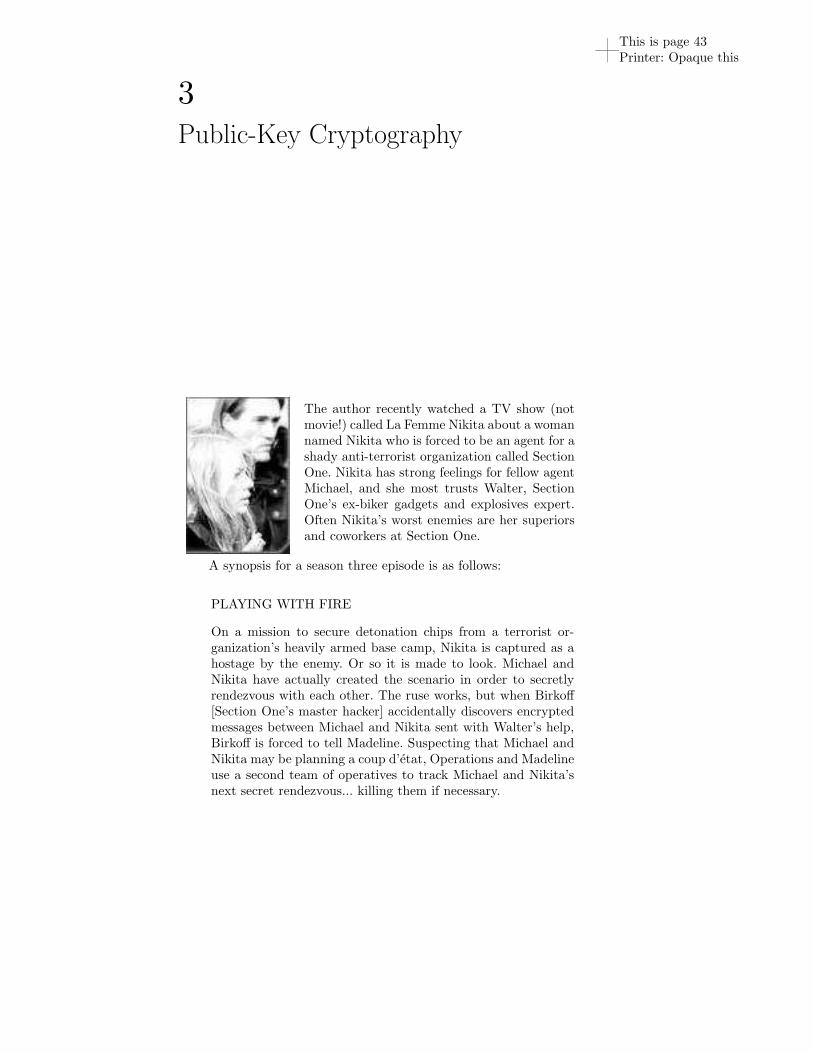
The author recently watched a TV show (notmovie!) called La Femme Nikita about a womannamed Nikita who is forced to be an agent for ashady anti-terrorist organization called SectionOne. Nikita has strong feelings for fellow agentMichael, and she most trusts Walter, SectionOne’s ex-biker gadgets and explosives expert.Often Nikita’s worst enemies are her superiorsand coworkers at Section One.
A synopsis for a season three episode is as follows:
PLAYING WITH FIRE
On a mission to secure detonation chips from a terrorist or-ganization’s heavily armed base camp, Nikita is captured as ahostage by the enemy. Or so it is made to look. Michael andNikita have actually created the scenario in order to secretlyrendezvous with each other. The ruse works, but when Birkoff[Section One’s master hacker] accidentally discovers encryptedmessages between Michael and Nikita sent with Walter’s help,Birkoff is forced to tell Madeline. Suspecting that Michael andNikita may be planning a coup d’etat, Operations and Madelineuse a second team of operatives to track Michael and Nikita’snext secret rendezvous... killing them if necessary.
44 3. Public-Key Cryptography
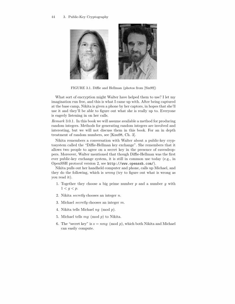
FIGURE 3.1. Diffie and Hellman (photos from [Sin99])
What sort of encryption might Walter have helped them to use? I let myimagination run free, and this is what I came up with. After being capturedat the base camp, Nikita is given a phone by her captors, in hopes that she’lluse it and they’ll be able to figure out what she is really up to. Everyoneis eagerly listening in on her calls.
Remark 3.0.1. In this book we will assume available a method for producingrandom integers. Methods for generating random integers are involved andinteresting, but we will not discuss them in this book. For an in depthtreatment of random numbers, see [Knu98, Ch. 3].
Nikita remembers a conversation with Walter about a public-key cryp-tosystem called the “Diffie-Hellman key exchange”. She remembers that itallows two people to agree on a secret key in the presence of eavesdrop-pers. Moreover, Walter mentioned that though Diffie-Hellman was the firstever public-key exchange system, it is still in common use today (e.g., inOpenSSH protocol version 2, see http://www.openssh.com/).
Nikita pulls out her handheld computer and phone, calls up Michael, andthey do the following, which is wrong (try to figure out what is wrong asyou read it).
1. Together they choose a big prime number p and a number g with1 < g < p.
2. Nikita secretly chooses an integer n.
3. Michael secretly chooses an integer m.
4. Nikita tells Michael ng (mod p).
5. Michael tells mg (mod p) to Nikita.
6. The “secret key” is s = nmg (mod p), which both Nikita and Michaelcan easily compute.
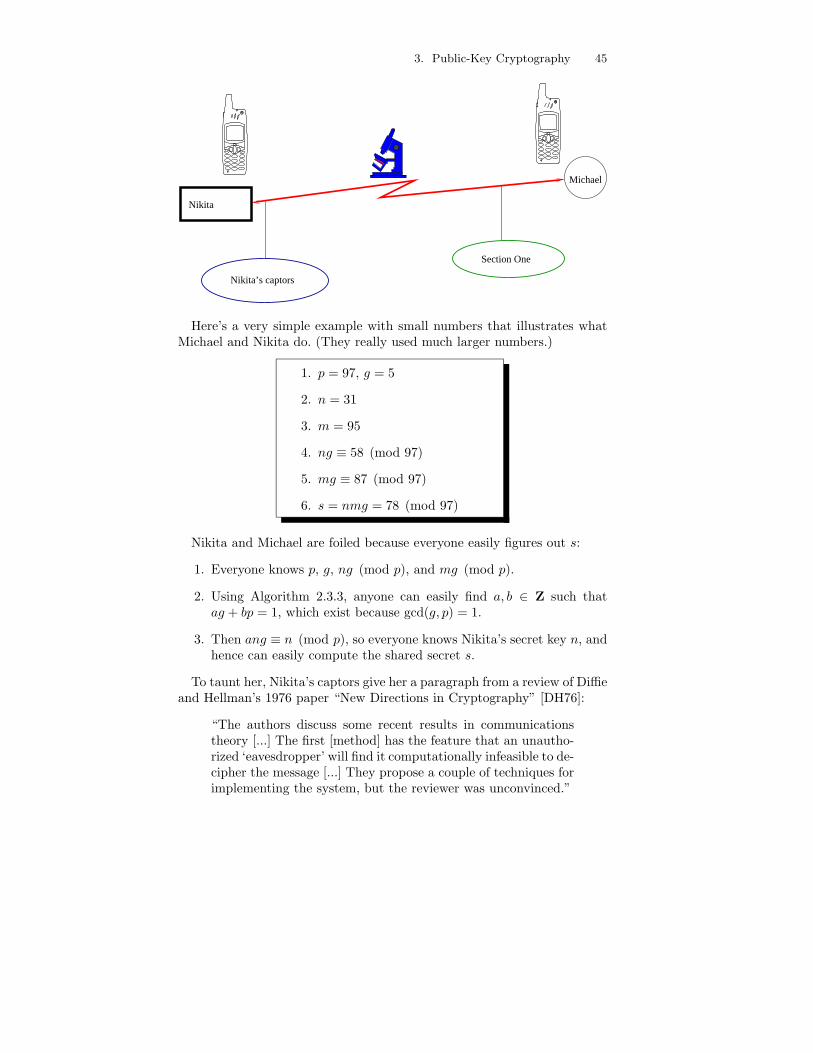
3. Public-Key Cryptography 45
Nikita
Michael
Nikita’s captors
Section One
Here’s a very simple example with small numbers that illustrates whatMichael and Nikita do. (They really used much larger numbers.)
1. p = 97, g = 5
2. n = 31
3. m = 95
4. ng ≡ 58 (mod 97)
5. mg ≡ 87 (mod 97)
6. s = nmg = 78 (mod 97)
Nikita and Michael are foiled because everyone easily figures out s:
1. Everyone knows p, g, ng (mod p), and mg (mod p).
2. Using Algorithm 2.3.3, anyone can easily find a, b ∈ Z such thatag + bp = 1, which exist because gcd(g, p) = 1.
3. Then ang ≡ n (mod p), so everyone knows Nikita’s secret key n, andhence can easily compute the shared secret s.
To taunt her, Nikita’s captors give her a paragraph from a review of Diffieand Hellman’s 1976 paper “New Directions in Cryptography” [DH76]:
“The authors discuss some recent results in communicationstheory [...] The first [method] has the feature that an unautho-rized ‘eavesdropper’ will find it computationally infeasible to de-cipher the message [...] They propose a couple of techniques forimplementing the system, but the reviewer was unconvinced.”
46 3. Public-Key Cryptography
3.1 The Diffie-Hellman Key Exchange
As night darkens Nikita’s cell, she reflects on what has happened. Upon re-alizing that she mis-remembered how the system works, she phones Michaeland they do the following:
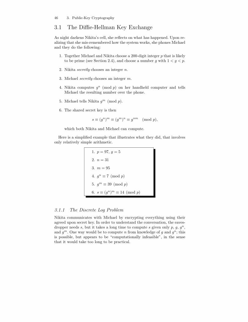
1. Together Michael and Nikita choose a 200-digit integer p that is likelyto be prime (see Section 2.4), and choose a number g with 1 < g < p.
2. Nikita secretly chooses an integer n.
3. Michael secretly chooses an integer m.
4. Nikita computes gn (mod p) on her handheld computer and tellsMichael the resulting number over the phone.
5. Michael tells Nikita gm (mod p).
6. The shared secret key is then
s ≡ (gn)m ≡ (gm)n ≡ gnm (mod p),
which both Nikita and Michael can compute.
Here is a simplified example that illustrates what they did, that involvesonly relatively simple arithmetic.
1. p = 97, g = 5
2. n = 31
3. m = 95
4. gn ≡ 7 (mod p)
5. gm ≡ 39 (mod p)
6. s ≡ (gn)m ≡ 14 (mod p)
3.1.1 The Discrete Log Problem
Nikita communicates with Michael by encrypting everything using theiragreed upon secret key. In order to understand the conversation, the eaves-dropper needs s, but it takes a long time to compute s given only p, g, gn,and gm. One way would be to compute n from knowledge of g and gn; thisis possible, but appears to be “computationally infeasible”, in the sensethat it would take too long to be practical.
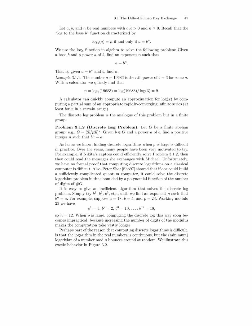
3.1 The Diffie-Hellman Key Exchange 47
Let a, b, and n be real numbers with a, b > 0 and n ≥ 0. Recall that the“log to the base b” function characterized by
logb(a) = n if and only if a = bn.
We use the logb function in algebra to solve the following problem: Givena base b and a power a of b, find an exponent n such that
a = bn.
That is, given a = bn and b, find n.
Example 3.1.1. The number a = 19683 is the nth power of b = 3 for some n.With a calculator we quickly find that
n = log3(19683) = log(19683)/ log(3) = 9.
A calculator can quickly compute an approximation for log(x) by com-puting a partial sum of an appropriate rapidly-converging infinite series (atleast for x in a certain range).
The discrete log problem is the analogue of this problem but in a finitegroup:
Problem 3.1.2 (Discrete Log Problem). Let G be a finite abeliangroup, e.g., G = (Z/pZ)∗. Given b ∈ G and a power a of b, find a positiveinteger n such that bn = a.
As far as we know, finding discrete logarithms when p is large is difficultin practice. Over the years, many people have been very motivated to try.For example, if Nikita’s captors could efficiently solve Problem 3.1.2, thenthey could read the messages she exchanges with Michael. Unfortunately,we have no formal proof that computing discrete logarithms on a classicalcomputer is difficult. Also, Peter Shor [Sho97] showed that if one could builda sufficiently complicated quantum computer, it could solve the discretelogarithm problem in time bounded by a polynomial function of the numberof digits of #G.
It is easy to give an inefficient algorithm that solves the discrete logproblem. Simply try b1, b2, b3, etc., until we find an exponent n such thatbn = a. For example, suppose a = 18, b = 5, and p = 23. Working modulo23 we have
b1 = 5, b2 = 2, b3 = 10, . . . , b12 = 18,
so n = 12. When p is large, computing the discrete log this way soon be-comes impractical, because increasing the number of digits of the modulusmakes the computation take vastly longer.
Perhaps part of the reason that computing discrete logarithms is difficult,is that the logarithm in the real numbers is continuous, but the (minimum)logarithm of a number mod n bounces around at random. We illustrate thisexotic behavior in Figure 3.2.
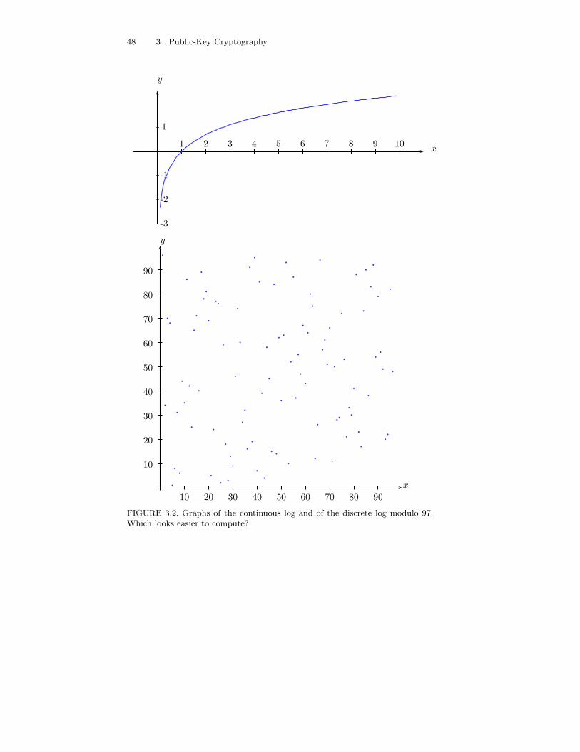
48 3. Public-Key Cryptography
x
y
1 2 3 4 5 6 7 8 9 10
-3
-2
-1
1
x
y
10 20 30 40 50 60 70 80 90
10
20
30
40
50
60
70
80
90
FIGURE 3.2. Graphs of the continuous log and of the discrete log modulo 97.Which looks easier to compute?
3.1 The Diffie-Hellman Key Exchange 49
3.1.2 Realistic Diffie-Hellman Example
In this section we present an example that uses bigger numbers. First weprove a proposition that we can use to choose a prime p in such a way thatit is easy to find a g ∈ (Z/pZ)∗ with order p − 1. We have already seen inSection 2.5 that for every prime p there exists an element g of order p− 1,and we gave Algorithm 2.5.13 for finding a primitive root for any prime.The significance of the proposition below is that it suggests an algorithmfor finding a primitive root that is easier to use in practice when p is large,because it does not require factoring p−1. Of course, one could also just usea random g for Diffie-Hellman; it is not essential that g generates (Z/pZ)∗.
Proposition 3.1.3. Suppose p is a prime such that (p−1)/2 is also prime.Then the elements of (Z/pZ)∗ have order either 1, 2, (p − 1)/2, or p − 1.
Proof. Since p is prime, the group (Z/pZ)∗ has order p−1. By assumption,the prime factorization of p − 1 is 2 · ((p − 1)/2). Let a ∈ (Z/pZ)∗. Thenby Theorem 2.1.12, ap−1 = 1, so the order of a is a divisor of p − 1, whichproves the proposition.
Given a prime p with (p − 1)/2 prime, find an element of order p − 1 asfollows. If 2 has order p− 1 we are done. If not, 2 has order (p− 1)/2 since2 doesn’t have order either 1 or 2. Then −2 has order p − 1.
Let p = 93450983094850938450983409611. Then p is prime, but (p −1)/2 is not. So we keep adding 2 to p and testing pseudoprimality usingSection 2.4 until we find that the next pseudoprime after p is
q = 93450983094850938450983409623.
It turns out that q pseudoprime and (q − 1)/2 is also pseudoprime. Wefind that 2 has order (q − 1)/2, so g = −2 has order q − 1 and is hence agenerator of (Z/qZ)∗, at least assuming that q is really prime.
The secret random numbers generated by Nikita and Michael are
n = 18319922375531859171613379181
andm = 82335836243866695680141440300.
Nikita sends
gn = 45416776270485369791375944998 ∈ (Z/pZ)∗
to Michael, and Michael sends
gm = 15048074151770884271824225393 ∈ (Z/pZ)∗
to Nikita. They agree on the secret key
gnm = 85771409470770521212346739540 ∈ (Z/pZ)∗.
Remark 3.1.4. See Section 7.3.1 for a computer implementation of theDiffie-Hellman key exchange.
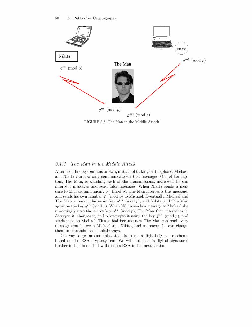
50 3. Public-Key Cryptography
Michael
Nikita
The Mangnt (mod p)
gnt (mod p)
gmt (mod p)
gmt (mod p)
FIGURE 3.3. The Man in the Middle Attack
3.1.3 The Man in the Middle Attack
After their first system was broken, instead of talking on the phone, Michaeland Nikita can now only communicate via text messages. One of her cap-tors, The Man, is watching each of the transmissions; moreover, he canintercept messages and send false messages. When Nikita sends a mes-sage to Michael announcing gn (mod p), The Man intercepts this message,and sends his own number gt (mod p) to Michael. Eventually, Michael andThe Man agree on the secret key gtm (mod p), and Nikita and The Managree on the key gtn (mod p). When Nikita sends a message to Michael sheunwittingly uses the secret key gtn (mod p); The Man then intercepts it,decrypts it, changes it, and re-encrypts it using the key gtm (mod p), andsends it on to Michael. This is bad because now The Man can read everymessage sent between Michael and Nikita, and moreover, he can changethem in transmission in subtle ways.
One way to get around this attack is to use a digital signature schemebased on the RSA cryptosystem. We will not discuss digital signaturesfurther in this book, but will discuss RSA in the next section.
3.2 The RSA Cryptosystem 51
3.2 The RSA Cryptosystem
The Diffie-Hellman key exchange has drawbacks. As discussed in Section3.1.3, it is susceptible to the man in the middle attack. This section isabout the RSA public-key cryptosystem of Rivest, Shamir, and Adleman[RSA78], which is an alternative to Diffie-Hellman that is more flexible insome ways.
We first describe the RSA cryptosystem, then discuss several ways toattack it. It is important to be aware of such weaknesses, in order to avoidfoolish mistakes when implementing RSA. We barely scratched the surfacehere of the many possible attacks on specific implementations of RSA orother cryptosystems.
3.2.1 How RSA works
The fundamental idea behind RSA is to try to construct a trap-door orone-way function on a set X, that is, an invertible function
E : X → X
such that it is easy for Nikita to compute E−1, but extremely difficult foranybody else to do so.
Here is how Nikita makes a one-way function E on the set of integersmodulo n.
1. Using a method hinted at in Section 2.4, Nikita picks two largeprimes p and q, and lets n = pq.
2. It is then easy for Nikita to compute
ϕ(n) = ϕ(p) · ϕ(q) = (p − 1) · (q − 1).
3. Nikita next chooses a random integer e with
1 < e < ϕ(n) and gcd(e, ϕ(n)) = 1.
4. Nikita uses the algorithm from Section 2.3.2 to find a solution x = dto the equation
ex ≡ 1 (mod ϕ(n)).
5. Finally, Nikita defines a function E : Z/nZ → Z/nZ by
E(x) = xe ∈ Z/nZ.
Anybody can compute E fairly quickly using the repeated-squaringalgorithm from Section 2.3.2.
52 3. Public-Key Cryptography
Nikita’s public key is the pair of integers (n, e), which is just enoughinformation for people to easily compute E. Nikita knows a number d suchthat ed ≡ 1 (mod ϕ(n)), so, as we will see, she can quickly compute E−1.
To send Nikita a message, proceed as follows. Encode your message, insome way, as a sequence of numbers modulo n (see Section 3.2.2)
m1, . . . ,mr ∈ Z/nZ,
then sendE(m1), . . . , E(mr)
to Nikita. (Recall that E(m) = me for m ∈ Z/nZ.)When Nikita receives E(mi), she finds each mi by using that E−1(m) =
md, a fact that follows from the following proposition.
Proposition 3.2.1 (Decryption key). Let n be an integer that is aproduct of distinct primes and let d, e ∈ N be such that p − 1 | de − 1 foreach prime p | n. Then ade ≡ a (mod n) for all a ∈ Z.
Proof. Since n | ade − a if and only if p | ade − a for each prime divisor pof n, it suffices to prove that ade ≡ a (mod p) for each prime divisor p of n.If gcd(a, p) 6= 0, then a ≡ 0 (mod p), so ade ≡ a (mod p). If gcd(a, p) = 1,then Theorem 2.1.12 asserts that ap−1 ≡ 1 (mod p). Since p − 1 | de − 1,we have ade−1 ≡ 1 (mod p) as well. Multiplying both sides by a shows thatade ≡ a (mod p).
Thus to decrypt E(mi) Nikita computes
E(mi)d = (me
i )d = mi.
For an implementation of RSA see Section 7.3.3.
3.2.2 Encoding a Phrase in a Number
In order to use the RSA cryptosystem to encrypt messages, it is necessaryto encode them as a sequence of numbers of size less than n = pq. We nowdescribe a simple way to do this. For an implementation of a slightly moregeneral encoding that includes extra randomness so that plain text encodesdifferently each time, see Section 7.3.2.
Suppose s is a sequence of capital letters and spaces, and that s does notbegin with a space. We encode s as a number in base 27 as follows: a singlespace corresponds to 0, the letter A to 1, B to 2, . . ., Z to 26. Thus “RUNNIKITA” is a number written in base 27:
RUN NIKITA ↔ 279 · 18 + 278 · 21 + 277 · 14 + 276 · 0 + 275 · 14
+ 274 · 9 + 273 · 11 + 272 · 9 + 27 · 20 + 1
= 143338425831991 (in decimal).
3.2 The RSA Cryptosystem 53
To recover the letters from the decimal number, repeatedly divide by 27and read off the letter corresponding to each remainder:
143338425831991 = 5308830586370 · 27 + 1 “A”5308830586370 = 196623355050 · 27 + 20 “T”196623355050 = 7282346483 · 27 + 9 “I”
7282346483 = 269716536 · 27 + 11 “K”269716536 = 9989501 · 27 + 9 “I”
9989501 = 369981 · 27 + 14 “N”369981 = 13703 · 27 + 0 “ ”13703 = 507 · 27 + 14 “N”
507 = 18 · 27 + 21 “U”18 = 0 · 27 + 18 “R”
If 27k ≤ n, then any sequence of k letters can be encoded as above usinga positive integer ≤ n. Thus if we use can encrypt integers of size at most n,then we must break our message up into blocks of size at most log27(n).
3.2.3 Examples
So the arithmetic is easy to follow, we use small primes p and q and encryptthe single letter “X” using the RSA cryptosystem.
1. Choose p and q: Let p = 17, q = 19, so n = pq = 323.
2. Compute ϕ(n):
ϕ(n) = ϕ(p · q) = ϕ(p) · ϕ(q) = (p − 1)(q − 1)
= pq − p − q + 1 = 323 − 17 − 19 + 1 = 288.
3. Randomly choose an e < 288: We choose e = 95.
4. Solve
95x ≡ 1 (mod 288).
Using the GCD algorithm, we find that d = 191 solves the equation.
The public key is (323, 95), so the encryption function is
E(x) = x95,
and the decryption function is D(x) = x191.Next, we encrypt the letter “X”. It is encoded as the number 24, since X
is the 24th letter of the alphabet. We have
E(24) = 2495 = 294 ∈ Z/323Z.
54 3. Public-Key Cryptography
To decrypt, we compute E−1:
E−1(294) = 294191 = 24 ∈ Z/323Z.
This next example illustrates RSA but with bigger numbers. Let
p = 738873402423833494183027176953, q = 3787776806865662882378273.
Then
n = p · q = 2798687536910915970127263606347911460948554197853542169
and
ϕ(n) = (p − 1)(q − 1)
= 2798687536910915970127262867470721260308194351943986944.
Using a pseudo-random number generator on a computer, the author ran-domly chose the integer
e = 1483959194866204179348536010284716655442139024915720699.
Then
d = 2113367928496305469541348387088632973457802358781610803
Since log27(n) ≈ 38.04, we can encode then encrypt single blocks ofup to 38 letters. Let’s encrypt “RUN NIKITA”, which encodes as m =143338425831991. We have
E(m) = me
= 1504554432996568133393088878600948101773726800878873990.
Remark 3.2.2. In practice one usually choses e to be small, since that doesnot seem to reduce the security of RSA, and makes the key size smaller. Forexample, in the OpenSSL documentation (see http://www.openssl.org/)about their implementation of RSA it states that “The exponent is an oddnumber, typically 3, 17 or 65537.”
3.3 Attacking RSA
Suppose Nikita’s public key is (n, e) and her decryption key is d, so ed ≡ 1(mod ϕ(n)). If somehow we compute the factorization n = pq, then we cancompute ϕ(n) = (p−1)(q−1) and hence compute d. Thus if we can factor nthen we can break the corresponding RSA public-key cryptosystem.
3.3 Attacking RSA 55
3.3.1 Factoring n Given ϕ(n)
Suppose n = pq. Given ϕ(n), it is very easy to compute p and q. We have
ϕ(n) = (p − 1)(q − 1) = pq − (p + q) + 1,
so we know both pq = n and p + q = n + 1 − ϕ(n). Thus we know thepolynomial
x2 − (p + q)x + pq = (x − p)(x − q)
whose roots are p and q. These roots can be found using the quadraticformula.
Example 3.3.1. The number n = pq = 31615577110997599711 is a productof two primes, and ϕ(n) = 31615577098574867424. We have
f = x2 − (n + 1 − ϕ(n))x + n
= x2 − 12422732288x + 31615577110997599711
= (x − 3572144239)(x − 8850588049),
where the factorization step is easily accomplished using the quadraticformula:
−b +√
b2 − 4ac
2a
=12422732288 +
√124227322882 − 4 · 31615577110997599711
2= 8850588049.
We conclude that n = 3572144239 · 8850588049.
3.3.2 When p and q are Close
Suppose that p and q are “close” to each other. Then it is easy to factor nusing a factorization method of Fermat.
Suppose n = pq with p > q, say. Then
n =
(
p + q
2
)2
−(
p − q
2
)2
.
Since p and q are “close”,
s =p − q
2is small,
t =p + q
2
is only slightly larger than√
n, and t2 − n = s2 is a perfect square. So wejust try
t = ⌈√
n⌉, t = ⌈√
n⌉ + 1, t = ⌈√
n⌉ + 2, . . .
56 3. Public-Key Cryptography
until t2−n is a perfect square s2. (Here ⌈x⌉ denotes the least integer n ≥ x.)Then
p = t + s, q = t − s.
Example 3.3.2. Suppose n = 23360947609. Then
√n = 152842.88 . . . .
If t = 152843, then√
t2 − n = 187.18 . . ..If t = 152844, then
√t2 − n = 583.71 . . ..
If t = 152845, then√
t2 − n = 804 ∈ Z.Thus s = 804. We find that p = t + s = 153649 and q = t − s = 152041.
3.3.3 Factoring n Given d
In this section, we show that finding the decryption key d for an RSAcryptosystem is, in practice, at least as difficult as factoring n. We give aprobabilistic algorithm that given a decryption key determines the factor-ization of n.
Consider an RSA cryptosystem with modulus n and encryption key e.Suppose we somehow finding an integer d such that
aed ≡ a (mod n)
for all a. Then m = ed − 1 satisfies am ≡ 1 (mod n) for all a that arecoprime to n. As we saw in Section 3.3.1, knowing ϕ(n) leads directly to afactorization of n. Unfortunately, knowing d does not seem to lead easily toa factorization of n. However, there is a probabilistic procedure that, givenan m such that am ≡ 1 (mod n), will find a factorization of n with “highprobability” (we will not analyze the probability here).
Algorithm 3.3.3 (Probabilistic Algorithm to Factor n). Let n = pqbe the product of two distinct odd primes, and suppose m is an integer suchthat am ≡ 1 (mod n) for all a coprime to n. This probabilistic algorithmfactors n with “high probability”. In the steps below, a always denotes aninteger coprime to n = pq.
1. [Divide out powers of 2] If am/2 ≡ 1 (mod n) for several randomlychosen a, set m = m/2, and go to step 1, otherwise let a be such thatam/2 6≡ 1 (mod n).
2. [Compute GCD’s] Compute g = gcd(am/2 − 1, n).
3. [Terminate?] If g is a proper divisor of n, output g and terminate. Oth-erwise go to step 1 and choose a different a.
In step 1, note that m is even since (−1)m ≡ 1 (mod n), so it makes senseto consider m/2. It is not practical to determine whether or not am/2 ≡ 1(mod n) for all a, because it would require doing a computation for too
3.3 Attacking RSA 57
many a. Instead, we try a few random a; if am/2 ≡ 1 (mod n) for the awe check, we divide m by 2. Also note that if there exists even a single asuch that am/2 6≡ 1 (mod n), then half the a have this property, since thena 7→ am/2 is a surjective homomorphism (Z/nZ)∗ → {±1} and the kernelhas index 2.
Proposition 2.5.2 implies that if x2 ≡ 1 (mod p) then x = ±1 (mod p).In step 2, since (am/2)2 ≡ 1 (mod n), we also have (am/2)2 ≡ 1 (mod p)and (am/2)2 ≡ 1 (mod q), so am/2 ≡ ±1 (mod p) and am/2 ≡ ±1 (mod q).Since am/2 6≡ 1 (mod n), there are three possibilities for these signs, so withprobability 2/3, one of the following two possibilities occurs:
1. am/2 ≡ +1 (mod p) and am/2 ≡ −1 (mod q)
2. am/2 ≡ −1 (mod p) and am/2 ≡ +1 (mod q).
The only other possibility is that both signs are −1. In the first case,
p | am/2 − 1 but q ∤ am/2 − 1,
so gcd(am/2 − 1, pq) = p, and we have factored n. Similarly, in the secondcase, gcd(am/2 − 1, pq) = q, and we again factor n.
Example 3.3.4. Somehow we discover that the RSA cryptosystem with
n = 32295194023343 and e = 29468811804857
has decryption key d = 11127763319273. We use this information and Al-gorithm 3.3.3 to factor n. If
m = ed − 1 = 327921963064646896263108960,
then ϕ(pq) | m, so am ≡ 1 (mod n) for all a coprime to n. For each a ≤ 20we find that am/2 ≡ 1 (mod n), so we replace m by
m
2= 163960981532323448131554480.
Again, we find with this new m that for each a ≤ 20, am/2 ≡ 1 (mod n), sowe replace m by 81980490766161724065777240. Yet again, for each a ≤ 20,am/2 ≡ 1 (mod n), so we replace m by 40990245383080862032888620. Thisis enough, since 2m/2 ≡ 4015382800099 (mod n). Then
gcd(2m/2 − 1, n) = gcd(4015382800098, 32295194023343) = 737531,
and we have found a factor of n. Dividing, we find that
n = 737531 · 43788253.
58 3. Public-Key Cryptography
3.3.4 Further Remarks
If one were to implement an actual RSA cryptosystem, there are many ad-ditional tricks and ideas to keep in mind. For example, one can add someextra random letters to each block of text, so that a given string will en-crypt differently each time it is encrypted. This makes it more difficult foran attacker who knows the encrypted and plaintext versions of one messageto gain information about subsequent encrypted messages. For an exampleimplementation that incorporates this randomness, see Listing 7.3.4. In anyparticular implementation, there might be attacks that would be devastat-ing in practice, but which wouldn’t require factoring the RSA modulus.
RSA is in common use, e.g., it is used in OpenSSH protocol version 1(see http://www.openssh.com/).
We will consider the ElGamal cryptosystem in Sections 6.4.2. It has asimilar flavor to RSA, but is more flexible in some ways.
3.4 Exercises
3.1 This problem concerns encoding phrases using numbers using theencoding of Section 3.2.2. What is the longest that an arbitrary se-quence of letters (no spaces) can be if it must fit in a number that isless than 1020?
3.2 Suppose Michael creates an RSA cryptosystem with a very large mod-ulus n for which the factorization of n cannot be found in a reasonableamount of time. Suppose that Nikita sends messages to Michael byrepresenting each alphabetic character as an integer between 0 and 26(A corresponds to 1, B to 2, etc., and a space à to 0), then encryptseach number separately using Michael’s RSA cryptosystem. Is thismethod secure? Explain your answer.
3.3 For any n ∈ N, let σ(n) be the sum of the divisors of n; for example,σ(6) = 1 + 2 + 3 + 6 = 12 and σ(10) = 1 + 2 + 5 + 10 = 18. Supposethat n = pqr with p, q, and r distinct primes. Devise an “efficient”algorithm that given n, ϕ(n) and σ(n), computes the factorizationof n. For example, if n = 105, then p = 3, q = 5, and r = 7, so theinput to the algorithm would be
n = 105, ϕ(n) = 48, and σ(n) = 192,
and the output would be 3, 5, and 7.
For computational exercises about cryptosystems, see the exercises forChapter 7.
This is page 59Printer: Opaque this
4Quadratic Reciprocity
The linear equationax ≡ b (mod n)
has a solution if and only if gcd(a, n) divides b (see Proposition 2.1.9). Thischapter is about some amazing mathematics motivated by the search for acriterion for whether or not a quadratic equation
ax2 + bx + c ≡ 0 (mod n)
has a solution. In many cases, the Chinese Remainder Theorem and thequadratic formula reduce this question to the key question of whether agiven integer a is a perfect square modulo a prime p.
The quadratic reciprocity law of Gauss provides a precise answer to thefollowing question: For which primes p is the image of a in (Z/pZ)∗ aperfect square? Amazingly, the answer depends only on the reduction of pmodulo 4a.
There are over a hundred proofs of the quadratic reciprocity law (see[Lem] for a long list). We give two proofs. The first, which we give in Sec-tion 4.3, is completely elementary and involves keeping track of integerpoints in intervals. It is satisfying because one can understand every detailwithout much abstraction, but it is unsatisfying because it is difficult toconceptualize what is going on. In sharp contrast, our second proof, whichwe we give in Section 4.4, in more abstract and uses a conceptual develop-ment of properties of Gauss sums. You should read Sections 4.1 and 4.2,then at least one of Section 4.3 or Section 4.4, depending on your taste andhow much abstract algebra you know.
60 4. Quadratic Reciprocity
In Section 4.5, we return to the computational question of actually find-ing square roots and solving quadratic equations in practice.
4.1 Statement of the Quadratic Reciprocity Law
In this section we state the quadratic reciprocity law.
Definition 4.1.1 (Quadratic Residue). Fix a prime p. An integer anot divisible by p is quadratic residue modulo p if a is a square modulo p;otherwise, a is a quadratic nonresidue.
The quadratic reciprocity theorem connects the question of whether ornot a is a quadratic residue modulo p to the question of whether p is aquadratic residue modulo each of the prime divisors of a. To express itprecisely, we introduce some new notation.
Definition 4.1.2 (Legendre Symbol). Let p be an odd prime and let abe an integer coprime to p. Set
(
a
p
)
=
{
+1 if a is a quadratic residue, and
−1 otherwise.
We call this symbol the Legendre Symbol.
This notation is well entrenched in the literature, even though it is alsothe notation for “a divided by p”; be careful not to confuse the two.
Since(
ap
)
only depends on a (mod p), it makes sense to define(
ap
)
for
a ∈ Z/pZ to be(
ap
)
for any lift a of a to Z.
Lemma 4.1.3. The map ψ : (Z/pZ)∗ → {±1} given by ψ(a) =(
ap
)
is a
surjective group homomorphism.
Proof. By Theorem 2.5.5, G = (Z/pZ)∗ is a cyclic group of order p −1. Because p is odd, G has even order, so the subgroup H of squares of
elements of G has index 2 in G. Since(
ap
)
= 1 if and only if a ∈ H, we
see that ψ is the composition G → G/H ∼= {±1}, where we identify thenontrivial element of G/H with −1.
Remark 4.1.4. We could also prove that ψ is surjective without using that(Z/pZ)∗ is cyclic, as follows. If a ∈ (Z/pZ)∗ is a square, say a ≡ b2 (mod p),then a(p−1)/2 = bp−1 ≡ 1 (mod p), so a is a root of f = x(p−1)/2 − 1. ByProposition 2.5.2, the polynomial f has at most (p−1)/2 roots. Thus theremust be an a ∈ (Z/pZ)∗ that is not a root of f , and for that a, we have
ψ(a) =(
ap
)
= −1, and trivially ψ(1) = 1, so the map ψ is surjective. Note
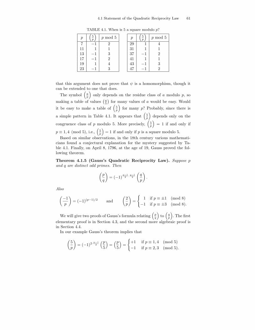
4.1 Statement of the Quadratic Reciprocity Law 61
TABLE 4.1. When is 5 a square modulo p?
p(
5p
)
p mod 5
7 −1 211 1 113 −1 317 −1 219 1 423 −1 3
p(
5p
)
p mod 5
29 1 431 1 137 −1 241 1 143 −1 347 −1 2
that this argument does not prove that ψ is a homomorphism, though itcan be extended to one that does.
The symbol(
ap
)
only depends on the residue class of a modulo p, so
making a table of values(
a5
)
for many values of a would be easy. Would
it be easy to make a table of(
5p
)
for many p? Probably, since there is
a simple pattern in Table 4.1. It appears that(
5p
)
depends only on the
congruence class of p modulo 5. More precisely,(
5p
)
= 1 if and only if
p ≡ 1, 4 (mod 5), i.e.,(
5p
)
= 1 if and only if p is a square modulo 5.
Based on similar observations, in the 18th century various mathemati-cians found a conjectural explanation for the mystery suggested by Ta-ble 4.1. Finally, on April 8, 1796, at the age of 19, Gauss proved the fol-lowing theorem.
Theorem 4.1.5 (Gauss’s Quadratic Reciprocity Law). Suppose pand q are distinct odd primes. Then
(
p
q
)
= (−1)p−12 · q−1
2
(
q
p
)
.
Also
(−1
p
)
= (−1)(p−1)/2 and
(
2
p
)
=
{
1 if p ≡ ±1 (mod 8)
−1 if p ≡ ±3 (mod 8).
We will give two proofs of Gauss’s formula relating(
pq
)
to(
qp
)
. The first
elementary proof is in Section 4.3, and the second more algebraic proof isin Section 4.4.
In our example Gauss’s theorem implies that
(
5
p
)
= (−1)2·p−12
(p
5
)
=(p
5
)
=
{
+1 if p ≡ 1, 4 (mod 5)
−1 if p ≡ 2, 3 (mod 5).
62 4. Quadratic Reciprocity
As an application, the following example illustrates how to answer ques-tions like “is a a square modulo b” using Theorem 4.1.5.
Example 4.1.6. Is 69 a square modulo the prime 389? We have(
69
389
)
=
(
3 · 23
389
)
=
(
3
389
)
·(
23
389
)
= (−1) · (−1) = 1.
Here(
3
389
)
=
(
389
3
)
=
(
2
3
)
= −1,
and(
23
389
)
=
(
389
23
)
=
(
21
23
)
=
(−2
23
)
=
(−1
23
)(
2
23
)
= (−1)23−1
2 · 1 = −1.
Thus 69 is a square modulo 389.Though we know that 69 is a square modulo 389, we don’t know an
explicit x such that x2 ≡ 69 (mod 389)! This is reminiscent of how we couldprove using Theorem 2.1.12 that certain numbers are composite withoutknowing a factorization.
Remark 4.1.7. The Jacobi symbol is an extension of the Legendre symbolto composite moduli. For more details, see Exercise 4.8.
4.2 Euler’s Criterion
Let p be an odd prime and a an integer not divisible by p. Euler used
the existence of primitive roots to show that(
ap
)
is congruent to a(p−1)/2
modulo p. We will use this fact repeatedly below in both proofs of Theo-rem 4.1.5.
Proposition 4.2.1 (Euler’s Criterion). We have(
ap
)
= 1 if and only
ifa(p−1)/2 ≡ 1 (mod p).
Proof. The map ϕ : (Z/pZ)∗ → (Z/pZ)∗ given by ϕ(a) = a(p−1)/2 isa group homomorphism, since powering is a group homomorphism of any
abelian group. Let ψ : (Z/pZ)∗ → {±1} be the homomorphism ψ(a) =(
ap
)
of Lemma 4.1.3. If a ∈ ker(ψ), then a = b2 for some b ∈ Z/pZ, so
ϕ(a) = a(p−1)/2 = (b2)(p−1)/2 = bp−1 = 1.
Thus ker(ψ) ⊂ ker(ϕ). By Lemma 4.1.3, ker(ψ) has index 2 in (Z/pZ)∗,so either ker(ϕ) = ker(ψ) or ϕ = 1. If ϕ = 1, the polynomial x(p−1)/2 − 1
4.3 First Proof of Quadratic Reciprocity 63
has p − 1 roots in the field Z/pZ, which contradicts Proposition 2.5.2, soker(ϕ) = ker(ψ), which proves the proposition.
From a computational point of view, Corollary 4.2.2 provides a conve-
nient way to compute(
ap
)
. See Section 7.4.1 for an implementation.
Corollary 4.2.2. The equation x2 ≡ a (mod p) has no solution if and
only if a(p−1)/2 ≡ −1 (mod p). Thus(
ap
)
≡ a(p−1)/2 (mod p).
Proof. This follows from Proposition 4.2.1 and the fact that the polyno-mial x2 − 1 has no roots besides +1 and −1 (which follows from Proposi-tion 2.5.3).
As additional computational motivation for the value of Corollary 4.2.2,
note that to evaluate(
ap
)
using Theorem 4.1.5 would not be practical
if a and p both very large, because it would require factoring a. However,
Corollary 4.2.2 provides a method for evaluating(
ap
)
without factoring a.
Example 4.2.3. Suppose p = 11. By squaring each element of (Z/11Z)∗, wesee that the squares modulo 11 are {1, 3, 4, 5, 9}. We compute a(p−1)/2 = a5
for each a ∈ (Z/11Z)∗ and get
15 = 1, 25 = −1, 35 = 1, 45 = 1, 55 = 1,
65 = −1, 75 = −1, 85 = −1, 95 = 1, 105 = −1.
Thus the a with a5 = 1 are {1, 3, 4, 5, 9}, just as Proposition 4.2.1 predicts.
Example 4.2.4. We determine whether or not 3 is a square modulo theprime p = 726377359. Using a computer we find that
3(p−1)/2 ≡ −1 (mod 726377359).
Thus 3 is not a square modulo p. This computation wasn’t difficult, but itwould have been tedious by hand. The law of quadratic reciprocity providesa way to answer this question, which could easily be carried out by hand:
(
3
726377359
)
= (−1)(3−1)/2·(726377359−1)/2
(
726377359
3
)
= (−1) ·(
1
3
)
= −1.
4.3 First Proof of Quadratic Reciprocity
Our first proof of quadratic reciprocity is elementary. The proof involveskeeping track of integer points in intervals. Proving Gauss’s lemma is the
64 4. Quadratic Reciprocity
first step; this lemma computes(
ap
)
in terms of the number of integers of
a certain type that lie in a certain interval. Next we prove Lemma 4.3.2,which controls how the parity of the number of integer points in an intervalchanges when an endpoint of the interval is changed. Then we prove that(
ap
)
depends only on p modulo 4a by applying Gauss’s lemma and keep-
ing careful track of intervals as they are rescaled and their endpoints arechanged. Finally, in Section 4.3.2 we use some basic algebra to deduce thequadratic reciprocity law using the tools we’ve just developed. Our prooffollows the one given in [Dav99] closely.
Lemma 4.3.1 (Gauss’s Lemma). Let p be an odd prime and let a be aninteger 6≡ 0 (mod p). Form the numbers
a, 2a, 3a, . . . ,p − 1
2a
and reduce them modulo p to lie in the interval (−p2 , p
2 ). Let ν be thenumber of negative numbers in the resulting set. Then
(
a
p
)
= (−1)ν .
Proof. In defining ν, we expressed each number in
S =
{
a, 2a, . . . ,p − 1
2a
}
as congruent to a number in the set{
1,−1, 2,−2, . . . ,p − 1
2,−p − 1
2
}
.
No number 1, 2, . . . , p−12 appears more than once, with either choice of sign,
because if it did then either two elements of S are congruent modulo p or0 is the sum of two elements of S, and both events are impossible. Thusthe resulting set must be of the form
T =
{
ε1 · 1, ε2 · 2, . . . , ε(p−1)/2 ·p − 1
2
}
,
where each εi is either +1 or −1. Multiplying together the elements of Sand of T , we see that
(1a) · (2a) · (3a) · · ·(
p − 1
2a
)
≡
(ε1 · 1) · (ε2 · 2) · · ·(
ε(p−1)/2 ·p − 1
2
)
(mod p),
soa(p−1)/2 ≡ ε1 · ε2 · · · ε(p−1)/2 (mod p).
The lemma then follows from Proposition 4.2.1, since(
ap
)
= a(p−1)/2.
4.3 First Proof of Quadratic Reciprocity 65
4.3.1 Euler’s Proposition
For rational numbers a, b ∈ Q, let
(a, b) ∩ Z = {x ∈ Z : a ≤ x ≤ b}
be the set of integers between a and b. The following lemma will help us tokeep track of how many integers lie in certain intervals.
Lemma 4.3.2. Let a, b ∈ Q. Then for any integer n,
#((a, b) ∩ Z) ≡ #((a, b + 2n) ∩ Z) (mod 2)
and#((a, b) ∩ Z) ≡ #((a − 2n, b) ∩ Z) (mod 2),
provided that each interval involved in the congruence is nonempty.
Note that if one of the intervals is empty, then the statement may befalse; e.g., if (a, b) = (−1/2, 1/2) and n = −1 then #((a, b) ∩ Z) = 1 but#(a, b − 2) ∩ Z = 0.
Proof. Let ⌈x⌉ denotes the least integer ≥ x. Since n > 0,
(a, b + 2n) = (a, b) ∪ [b, b + 2n),
where the union is disjoint. There are 2n integers,
⌈b⌉, ⌈b⌉ + 1, . . . , ⌈b⌉ + 2n − 1,
in the interval [b, b + 2n), so the first congruence of the lemma is true inthis case. We also have
(a, b − 2n) = (a, b) minus [b − 2n, b)
and [b−2n, b) contains exactly 2n integers, so the lemma is also true when nis negative. The statement about # ((a − 2n, b) ∩ Z) is proved in a similarmanner.
Once we have proved the following proposition, it will be easy to deducethe quadratic reciprocity law.
Proposition 4.3.3 (Euler). Let p be an odd prime and let a be a positive
integer with p ∤ a. If q is a prime with q ≡ ±p (mod 4a), then(
ap
)
=(
aq
)
.
Proof. We will apply Lemma 4.3.1 to compute(
ap
)
. Let
S =
{
a, 2a, 3a, . . . ,p − 1
2a
}
66 4. Quadratic Reciprocity
and
I =
(
1
2p, p
)
∪(
3
2p, 2p
)
∪ · · · ∪((
b − 1
2
)
p, bp
)
,
where b = 12a or 1
2 (a − 1), whichever is an integer. We check that everyelement of S that reduces to something in the interval (−p
2 , 0) lies in I.
This is clear if b = 12a < p−1
2 a. If b = 12 (a − 1), then bp + p
2 > p−12 a, so
((b − 12 )p, bp) is the last interval that could contain an element of S that
reduces to (−p2 , 0). Note that the integer endpoints of I are not in S, since
those endpoints are divisible by p, but no element of S is divisible by p.Thus, by Lemma 4.3.1,
(
a
p
)
= (−1)#(S∩I).
To compute #(S ∩ I), first rescale by a to see that
#(S ∩ I) = #
(
Z ∩ 1
aI
)
,
where
1
aI =
(
( p
2a,p
a
)
∪(
3p
2a,2p
a
)
∪ · · · ∪(
(2b − 1)p
2a,bp
a
))
.
Write p = 4ac + r, and let
J =
(
( r
2a,r
a
)
∪(
3r
2a,2r
a
)
∪ · · · ∪(
(2b − 1)r
2a,br
a
))
.
The only difference between I and J is that the endpoints of intervals arechanged by addition of an even integer. By Lemma 4.3.2,
ν = #
(
Z ∩ 1
aI
)
≡ #(Z ∩ J) (mod 2).
Thus(
ap
)
= (−1)ν depends only on r, i.e., only on p modulo 4a. Thus if
q ≡ p (mod 4a), then(
ap
)
=(
aq
)
.
If q ≡ −p (mod 4a), then the only change in the above computation isthat r is replaced by 4a − r. This changes 1
aI into
K =(
2 − r
2a, 4 − r
a
)
∪(
6 − 3r
2a, 8 − 2r
a
)
∪ · · ·
∪(
4b − 2 − (2b − 1)r
2a, 4b − br
a
)
.
4.3 First Proof of Quadratic Reciprocity 67
Thus K is the same as − 1aI, except even integers have been added to the
endpoints. By Lemma 4.3.2,
#(K ∩ Z) ≡ #
((
1
aI
)
∩ Z
)
(mod 2),
so(
ap
)
=(
aq
)
, which completes the proof.
The following more careful analysis in the special case when a = 2 helpsillustrate the proof of the above lemma, and the result is frequently useful incomputations. For an alternative proof of the proposition, see Exercise 4.5.
Proposition 4.3.4 (Legendre symbol of 2). Let p be an odd prime.Then
(
2
p
)
=
{
1 if p ≡ ±1 (mod 8)
−1 if p ≡ ±3 (mod 8).
Proof. When a = 2, the set S = {a, 2a, . . . , 2 · p−12 } is
{2, 4, 6, . . . , p − 1}.
We must count the parity of the number of elements of S that lie in theinterval I = (p
2 , p). Writing p = 8c + r, we have
# (I ∩ S) = #
(
1
2I ∩ Z
)
= #((p
4,p
2
)
∩ Z)
= #((
2c +r
4, 4c +
r
2
)
∩ Z)
≡ #((r
4,r
2
)
∩ Z)
(mod 2),
where the last equality comes from Lemma 4.3.2. The possibilities for r are1, 3, 5, 7. When r = 1, the cardinality is 0, when r = 3, 5 it is 1, and whenr = 7 it is 2.
4.3.2 Proof of Quadratic Reciprocity
It is now straightforward to deduce the quadratic reciprocity law.
First Proof of Theorem 4.1.5. First suppose that p ≡ q (mod 4). By swap-ping p and q if necessary, we may assume that p > q, and write p− q = 4a.Since p = 4a + q,
(
p
q
)
=
(
4a + q
q
)
=
(
4a
q
)
=
(
4
q
) (
a
q
)
=
(
a
q
)
,
and(
q
p
)
=
(
p − 4a
p
)
=
(−4a
p
)
=
(−1
p
)
·(
a
p
)
.
68 4. Quadratic Reciprocity
Proposition 4.3.3 implies that(
aq
)
=(
ap
)
, since p ≡ q (mod 4a). Thus
(
p
q
)
·(
q
p
)
=
(−1
p
)
= (−1)p−12 = (−1)
p−12 · q−1
2 ,
where the last equality is because p−12 is even if and only if q−1
2 is even.Next suppose that p 6≡ q (mod 4), so p ≡ −q (mod 4). Write p+ q = 4a.
We have(
p
q
)
=
(
4a − q
q
)
=
(
a
q
)
, and
(
q
p
)
=
(
4a − p
p
)
=
(
a
p
)
.
Since p ≡ −q (mod 4a), Proposition 4.3.3 implies that(
pq
)
=(
qp
)
. Since
(−1)p−12 · q−1
2 = 1, the proof is complete.
4.4 A Proof of Quadratic Reciprocity Using GaussSums
In this section we present a beautiful proof of Theorem 4.1.5 using algebraicidentities satisfied by sums of “roots of unity”. The objects we introducein the proof are of independent interest, and provide a powerful tool toprove higher-degree analogues of quadratic reciprocity. (For more on higherreciprocity see [IR90]. See also Section 6 of [IR90] on which the proof belowis modeled.)
Definition 4.4.1 (Root of Unity). An nth root of unity is a complexnumber ζ such that ζn = 1. A root of unity ζ is a primitive nth root ofunity if n is the smallest positive integer such that ζn = 1.
For example, −1 is a primitive second root of unity, and ζ =√−3−12 is
a primitive cube root of unity. More generally, for any n ∈ N the complexnumber
ζn = cos(2π/n) + i sin(2π/n)
is a primitive nth root of unity (this follows from the identity eiθ = cos(θ)+i sin(θ)). For the rest of this section, we fix an odd prime p and the primitivepth root ζ = ζp of unity.
Definition 4.4.2 (Gauss Sum). Fix an odd prime p. The Gauss sumassociated to an integer a is
ga =
p−1∑
n=0
(
n
p
)
ζan,
where ζ = ζp = cos(2π/p) + i sin(2π/p).
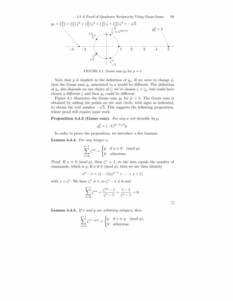
4.4 A Proof of Quadratic Reciprocity Using Gauss Sums 69
−1
+1
+1
−1
ζ = e2πi/5
ζ2
ζ3
ζ4
g2 =(
05
)
+(
15
)
ζ2 +(
25
)
ζ4 +(
35
)
ζ +(
45
)
ζ3 = −√
5
g22 = 5
1 2 3 4 5−3 −2
FIGURE 4.1. Gauss sum g2 for p = 5
Note that p is implicit in the definition of ga. If we were to change p,then the Gauss sum ga associated to a would be different. The definitionof ga also depends on our choice of ζ; we’ve chosen ζ = ζp, but could havechosen a different ζ and then ga could be different.
Figure 4.1 illustrates the Gauss sum g2 for p = 5. The Gauss sum isobtained by adding the points on the unit circle, with signs as indicated,to obtain the real number −
√5. This suggests the following proposition,
whose proof will require some work.
Proposition 4.4.3 (Gauss sum). For any a not divisible by p,
g2a = (−1)(p−1)/2p.
In order to prove the proposition, we introduce a few lemmas.
Lemma 4.4.4. For any integer a,
p−1∑
n=0
ζan =
{
p if a ≡ 0 (mod p),
0 otherwise.
Proof. If a ≡ 0 (mod p), then ζa = 1, so the sum equals the number ofsummands, which is p. If a 6≡ 0 (mod p), then we use then identity
xp − 1 = (x − 1)(xp−1 + · · · + x + 1)
with x = ζa. We have ζa 6= 1, so ζa − 1 6= 0 and
p−1∑
n=0
ζan =ζap − 1
ζa − 1=
1 − 1
ζa − 1= 0.
Lemma 4.4.5. If x and y are arbitrary integers, then
p−1∑
n=0
ζ(x−y)n =
{
p if x ≡ y (mod p),
0 otherwise.
70 4. Quadratic Reciprocity
Proof. This follows from Lemma 4.4.4 by setting a = x − y.
Lemma 4.4.6. We have g0 = 0.
Proof. By definition
g0 =
p−1∑
n=0
(
n
p
)
. (4.4.1)
By Lemma 4.1.3, the map
( ·p
)
: (Z/pZ)∗ → {±1}
is a surjective homomorphism of groups. Thus half the elements of (Z/pZ)∗
map to +1 and half map to −1 (the subgroup that maps to +1 has index
2). Since(
0p
)
= 0, the sum (4.4.1) is 0.
Lemma 4.4.7. For any integer a,
ga =
(
a
p
)
g1.
Proof. When a ≡ 0 (mod p) the lemma follows from Lemma 4.4.6, so sup-pose that a 6≡ 0 (mod p). Then
(
a
p
)
ga =
(
a
p
) p−1∑
n=0
(
n
p
)
ζan =
p−1∑
n=0
(
an
p
)
ζan =
p−1∑
m=0
(
m
p
)
ζm = g1.
Here we use that multiplication by a is an automorphism of Z/pZ. Finally,
multiply both sides by(
ap
)
and use that(
ap
)2
= 1.
We have enough lemmas to prove Proposition 4.4.3.
Proof of Proposition 4.4.3. We evaluate the sum∑p−1
a=0 gag−a in two dif-ferent ways. By Lemma 4.4.7, since a 6≡ 0 (mod p) we have
gag−a =
(
a
p
)
g1
(−a
p
)
g1 =
(−1
p
)(
a
p
)2
g21 = (−1)(p−1)/2g2
1 ,
where the last step follows from Proposition 4.2.1 and that(
ap
)
∈ {±1}.Thus
p−1∑
a=0
gag−a = (p − 1)(−1)(p−1)/2g21 . (4.4.2)
4.4 A Proof of Quadratic Reciprocity Using Gauss Sums 71
On the other hand, by definition
gag−a =
p−1∑
n=0
(
n
p
)
ζan ·p−1∑
m=0
(
m
p
)
ζ−am
=
p−1∑
n=0
p−1∑
m=0
(
n
p
) (
m
p
)
ζanζ−am
=
p−1∑
n=0
p−1∑
m=0
(
n
p
) (
m
p
)
ζan−am.
Let δ(n,m) = 1 if n ≡ m (mod p) and 0 otherwise. By Lemma 4.4.5,
p−1∑
a=0
gag−a =
p−1∑
a=0
p−1∑
n=0
p−1∑
m=0
(
n
p
) (
m
p
)
ζan−am
=
p−1∑
n=0
p−1∑
m=0
(
n
p
)(
m
p
) p−1∑
a=0
ζan−am
=
p−1∑
n=0
p−1∑
m=0
(
n
p
)(
m
p
)
pδ(n,m)
=
p−1∑
n=0
(
n
p
)2
p
= p(p − 1).
Equate (4.4.2) and the above equality, then cancel (p − 1) to see that
g21 = (−1)(p−1)/2p.
Since a 6≡ 0 (mod p), we have(
ap
)2
= 1, so by Lemma 4.4.7,
g2a =
(
a
p
)2
g21 = g2
1 ,
and the proposition is proved.
4.4.1 Proof of Quadratic Reciprocity
We are now ready to prove Theorem 4.1.5 using Gauss sums.
Proof. Let q be an odd prime with q 6= p. Set p∗ = (−1)(p−1)/2p and recall
that Proposition 4.4.3 asserts that p∗ = g2, where g = g1 =∑p−1
n=0
(
np
)
ζn.
72 4. Quadratic Reciprocity
Proposition 4.2.1 implies that
(p∗)(q−1)/2 ≡(
p∗
q
)
(mod q).
We have gq−1 = (g2)(q−1)/2 = (p∗)(q−1)/2, so multiplying both sides of thedisplayed equation by g yields a congruence
gq ≡ g
(
p∗
q
)
(mod q). (4.4.3)
But wait, what does this congruence mean, given that gq is not an in-
teger? It means that the difference gq − g(
p∗
q
)
lies in the ideal (q) in the
ring Z[ζ] of all polynomials in ζ with coefficients in Z.The ring Z[ζ]/(q) has characteristic q, so if x, y ∈ Z[ζ], then (x + y)q ≡
xq + yq (mod q). Applying this to (4.4.3), we see that
gq =
(
p−1∑
n=0
(
n
p
)
ζn
)q
≡p−1∑
n=0
(
n
p
)q
ζnq ≡p−1∑
n=0
(
n
p
)
ζnq ≡ gq (mod q).
By Lemma 4.4.7,
gq ≡ gq ≡(
q
p
)
g (mod q).
Combining this with (4.4.3) yields
(
q
p
)
g ≡(
p∗
q
)
g (mod q).
Since g2 = p∗ and p 6= q, we can cancel g from both sides to find that(
qp
)
≡(
p∗
q
)
(mod q). Since both residue symbols are ±1 and q is odd, it
follows that(
qp
)
=(
p∗
q
)
. Finally, we note using Proposition 4.2.1 that
(
p∗
q
)
=
(
(−1)(p−1)/2p
q
)
=
(−1
q
)(p−1)/2 (
p
q
)
= (−1)q−12 · p−1
2 ·(
p
q
)
.
4.5 Finding Square Roots
[[something about schoof polynomial time algo!!!]] We return in thissection to the question of computing square roots. If K is a field in which
4.5 Finding Square Roots 73
2 6= 0, and a, b, c ∈ K, with a 6= 0, then the solutions to the quadraticequation ax2 + bx + c = 0 are
x =−b ±
√b2 − 4ac
2a.
Now assume K = Z/pZ, with p an odd prime. Using Theorem 4.1.5, wecan decide whether or not b2 − 4ac is a perfect square in Z/pZ, and hencewhether or not ax2 + bx + c = 0 has a solution in Z/pZ. However Theo-rem 4.1.5 says nothing about how to actually find a solution when there isone. Also, note that for this problem we do not need the full quadratic reci-procity law; in practice to decide whether an element of Z/pZ is a perfectsquare Proposition 4.2.1 is quite fast, in view of Section 2.3.
Suppose a ∈ Z/pZ is a nonzero quadratic residue. If p ≡ 3 (mod 4) then
b = ap+14 is a square root of a because
b2 = ap+12 = a
p−12 +1 = a
p−12 · a =
(
a
p
)
· a = a.
We can compute b in time polynomial in the number of digits of p usingthe powering algorithm of Section 2.3.
We do not know a deterministic polynomial-time algorithm to computea square root of a when p ≡ 1 (mod 4). The following is a standard prob-abilistic algorithm to compute a square root of a, which works well inpractice. Consider the quotient ring
R = (Z/pZ)[x]/(x2 − a),
by which we mean the following. We have
R = {u + vα : u, v ∈ Z/pZ}
with multiplication defined by
(u + vα)(z + wα) = (uz + awv) + (uw + vz)α.
Here α corresponds to the class of x in the quotient ring. Let b and c bethe square roots of a in Z/pZ (though we cannot easily compute b and cyet, we can consider them in order to deduce an algorithm to find them).We have ring homomorphisms f : R → Z/pZ and g : R → Z/pZ given byf(u + vα) = u + vb and g(u + vα) = u + vc. Together these define a ringisomorphism
ϕ : R −→ Z/pZ × Z/pZ
given by ϕ(u + vα) = (u + vb, u + vc). Choose in some way a randomelement z of (Z/pZ)∗, and define u, v ∈ Z/pZ by
u + vα = (1 + zα)p−12 ,
74 4. Quadratic Reciprocity
where we compute (1 + zα)p−12 quickly using an analogue of the binary
powering algorithm of Section 2.3.2. If v = 0 we try again with anotherrandom z. If v 6= 0 we can quickly find the desired square roots b and cas follows. The quantity u + vb is a (p − 1)/2 power in Z/pZ, so it equalseither 0, 1, or −1, so b = −u/v, (1−u)/v, or (−1−u)/v, respectively. Sincewe know u and v we can try each of −u/v, (1− u)/v, and (−1− u)/v andsee which is a square root of a.
We implement this algorithm in Section 7.4.2.
Example 4.5.1. Continuing Example 4.1.6, we find a square root of 69modulo 389. We apply the algorithm described above in the case p ≡ 1(mod 4). We first choose the random z = 24 and find that (1 + 24α)194 =−1. The coefficient of α in the power is 0, and we try again with z = 51.This time we have (1 + 51α)194 = 239α = u + vα. The inverse of 239 inZ/389Z is 153, so we consider the following three possibilities for a squareroot of 69:
−u
v= 0
1 − u
v= 153 − 1 − u
v= −153.
Thus 153 and −153 are the square roots of 69 in Z/389Z.
4.6 Exercises
4.1 Calculate the following by hand:(
397
)
,(
3389
)
,(
2211
)
, and(
5!7
)
.
4.2 Use Theorem 4.1.5 to show that for p ≥ 5 prime,
(
3
p
)
=
{
1 if p ≡ 1, 11 (mod 12),
−1 if p ≡ 5, 7 (mod 12).
4.3 (*) Use that (Z/pZ)∗ is cyclic to give a direct proof that(
−3p
)
= 1
when p ≡ 1 (mod 3). (Hint: There is an c ∈ (Z/pZ)∗ of order 3. Showthat (2c + 1)2 = −3.)
4.4 (*) If p ≡ 1 (mod 5), show directly that(
5p
)
= 1 by the method of
Exercise 4.3. (Hint: Let c ∈ (Z/pZ)∗ be an element of order 5. Showthat (c + c4)2 + (c + c4) − 1 = 0, etc.)
4.5 (*) Let p be an odd prime. In this exercise you will prove that(
2p
)
= 1
if and only if p ≡ ±1 (mod 8).
(a) Prove that
x =1 − t2
1 + t2, y =
2t
1 + t2

4.6 Exercises 75
is a parameterization of the set of solutions to x2 + y2 ≡ 1(mod p), in the sense that the solutions (x, y) ∈ Z/pZ are inbijection with the t ∈ Z/pZ∪{∞} such that 1+t2 6≡ 0 (mod p).Here t = ∞ corresponds to the point (−1, 0). (Hint: if (x1, y1)is a solution, consider the line y = t(x + 1) through (x1, y1) and(−1, 0), and solve for x1, y1 in terms of t.)
(b) Prove that the number of solutions to x2 + y2 ≡ 1 (mod p) isp + 1 if p ≡ 3 (mod 4) and p − 1 if p ≡ 1 (mod 4).
(c) Consider the set S of pairs (a, b) ∈ (Z/pZ)∗×(Z/pZ)∗ such that
a + b = 1 and(
ap
)
=(
bp
)
= 1. Prove that #S = (p + 1 − 4)/4
if p ≡ 3 (mod 4) and #S = (p − 1 − 4)/4 if p ≡ 1 (mod 4).Conclude that #S is odd if and only if p ≡ ±1 (mod 8)
(d) The map σ(a, b) = (b, a) that swaps coordinates is a bijection ofthe set S. It has exactly one fixed point if and only if there is
an a ∈ Z/pZ such that 2a = 1 and(
ap
)
= 1. Also, prove that
2a = 1 has a solution a ∈ Z/pZ with(
ap
)
= 1 if and only if(
2p
)
= 1.
(e) Finish by showing that σ has exactly one fixed point if and onlyif #S is odd, i.e., if and only if p ≡ ±1 (mod 8).
Remark: The method of proof of this exercise can be generalized togive a proof of the full quadratic reciprocity law.
4.6 How many natural numbers x < 213 satisfy the equation
x2 ≡ 5 (mod 213 − 1)?
You may assume that 213 − 1 is prime.
4.7 Find the natural number x < 97 such that x ≡ 448 (mod 97). Notethat 97 is prime.
4.8 In this problem we will formulate an analogue of quadratic reciprocity
for a symbol like(
aq
)
, but without the restriction that q be a prime.
Suppose n is a positive integer, which we factor as∏k
i=1 pei
i . We definethe Jacobi symbol
(
an
)
as follows:
(a
n
)
=
k∏
i=1
(
a
pi
)ei
.
(a) Give an example to show that(
an
)
= 1 need not imply that a isa perfect square modulo n.
76 4. Quadratic Reciprocity
(b) (*) Let n be odd and a and b be integers. Prove that the followingholds:
i.(
an
) (
bn
)
=(
abn
)
. (Thus a 7→(
an
)
induces a homomorphismfrom (Z/nZ)∗ to {±1}.)
ii.(−1
n
)
≡ n (mod 4).
iii.(
2n
)
= 1 if n ≡ ±1 (mod 8) and −1 otherwise.
iv.(
an
)
= (−1)a−12 ·n−1
2
(
na
)
4.9 (*) Prove that for any n ∈ Z the integer n2 +n+1 does not have anydivisors of the form 6k − 1.
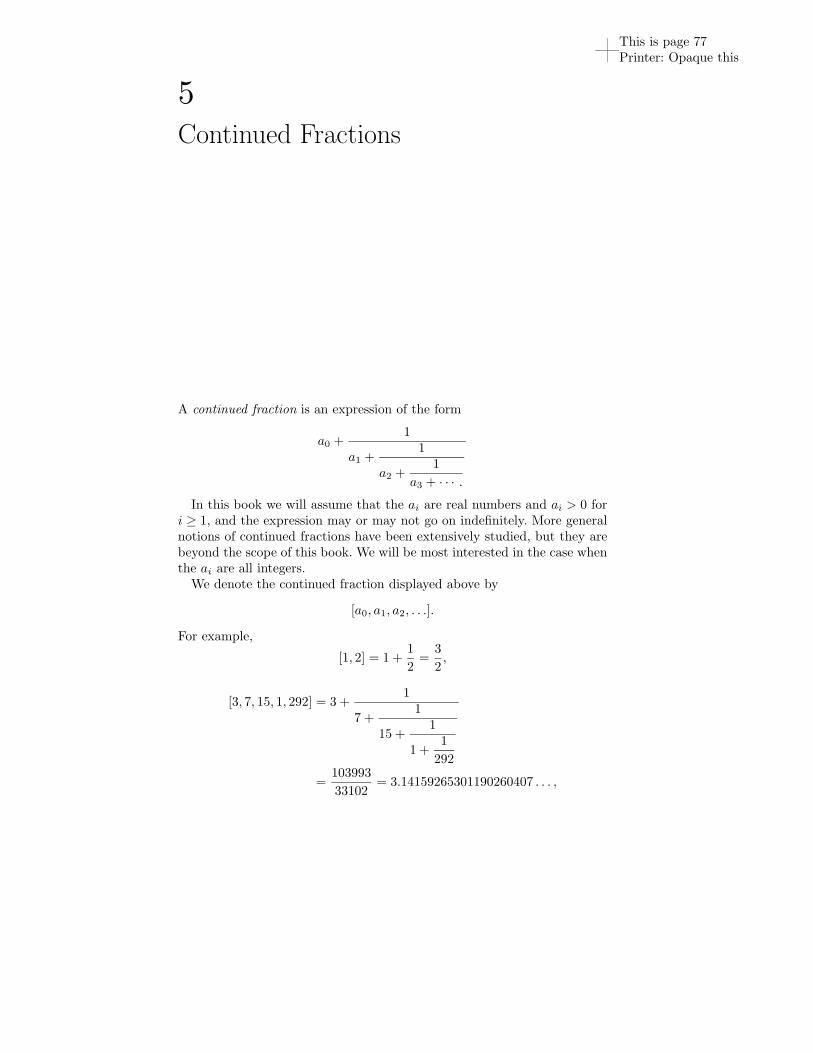
This is page 77Printer: Opaque this
5Continued Fractions
A continued fraction is an expression of the form
a0 +1
a1 +1
a2 +1
a3 + · · · .
In this book we will assume that the ai are real numbers and ai > 0 fori ≥ 1, and the expression may or may not go on indefinitely. More generalnotions of continued fractions have been extensively studied, but they arebeyond the scope of this book. We will be most interested in the case whenthe ai are all integers.
We denote the continued fraction displayed above by
[a0, a1, a2, . . .].
For example,
[1, 2] = 1 +1
2=
3
2,
[3, 7, 15, 1, 292] = 3 +1
7 +1
15 +1
1 +1
292
=103993
33102= 3.14159265301190260407 . . . ,
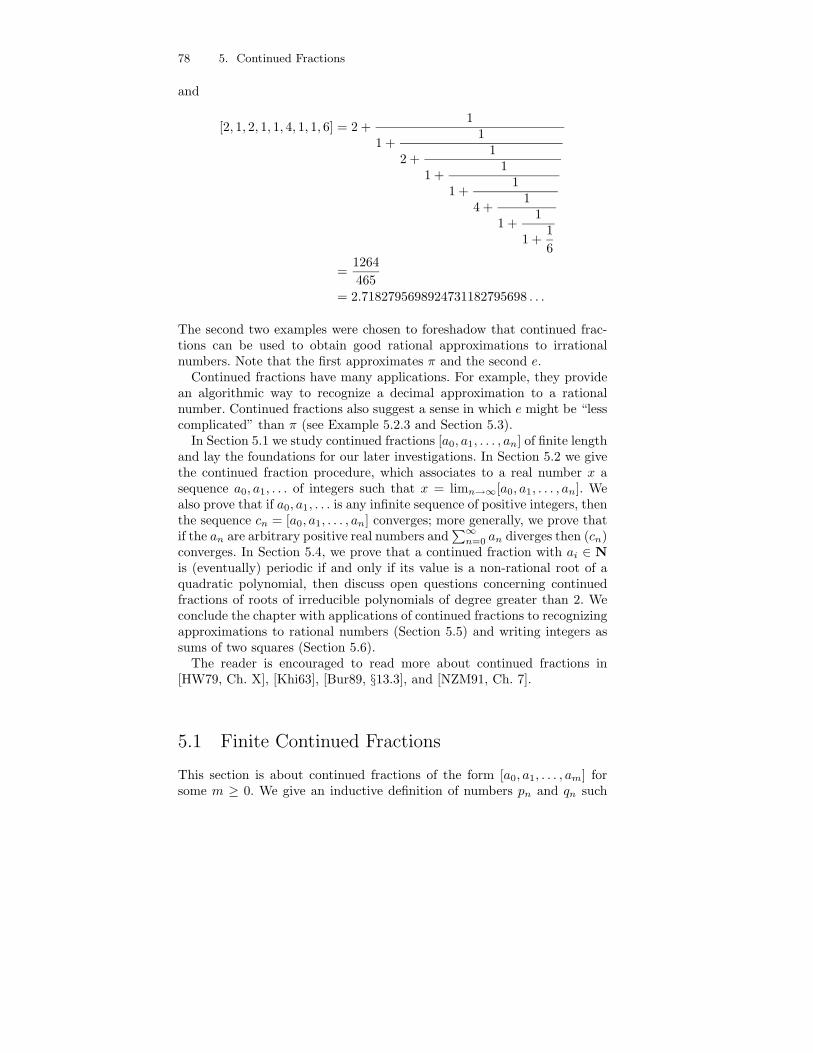
78 5. Continued Fractions
and
[2, 1, 2, 1, 1, 4, 1, 1, 6] = 2 +1
1 +1
2 +1
1 +1
1 +1
4 +1
1 +1
1 +1
6
=1264
465= 2.7182795698924731182795698 . . .
The second two examples were chosen to foreshadow that continued frac-tions can be used to obtain good rational approximations to irrationalnumbers. Note that the first approximates π and the second e.
Continued fractions have many applications. For example, they providean algorithmic way to recognize a decimal approximation to a rationalnumber. Continued fractions also suggest a sense in which e might be “lesscomplicated” than π (see Example 5.2.3 and Section 5.3).
In Section 5.1 we study continued fractions [a0, a1, . . . , an] of finite lengthand lay the foundations for our later investigations. In Section 5.2 we givethe continued fraction procedure, which associates to a real number x asequence a0, a1, . . . of integers such that x = limn→∞[a0, a1, . . . , an]. Wealso prove that if a0, a1, . . . is any infinite sequence of positive integers, thenthe sequence cn = [a0, a1, . . . , an] converges; more generally, we prove thatif the an are arbitrary positive real numbers and
∑∞n=0 an diverges then (cn)
converges. In Section 5.4, we prove that a continued fraction with ai ∈ Nis (eventually) periodic if and only if its value is a non-rational root of aquadratic polynomial, then discuss open questions concerning continuedfractions of roots of irreducible polynomials of degree greater than 2. Weconclude the chapter with applications of continued fractions to recognizingapproximations to rational numbers (Section 5.5) and writing integers assums of two squares (Section 5.6).
The reader is encouraged to read more about continued fractions in[HW79, Ch. X], [Khi63], [Bur89, §13.3], and [NZM91, Ch. 7].
5.1 Finite Continued Fractions
This section is about continued fractions of the form [a0, a1, . . . , am] forsome m ≥ 0. We give an inductive definition of numbers pn and qn such
5.1 Finite Continued Fractions 79
that for all n ≤ m
[a0, a1, . . . , an] =pn
qn. (5.1.1)
We then give related formulas for the determinants of the 2 × 2 matrices( pn pn−1
qn qn−1
)
and( pn pn−2
qn qn−2
)
. which we will repeatedly use to deduce prop-erties of the sequence of partial convergents [a0, . . . , ak]. We will use Al-gorithm 1.1.12 to prove that every rational number is represented by acontinued fraction, as in (5.1.1).
Definition 5.1.1 (Finite Continued Fraction). A finite continued frac-tion is an expression
a0 +1
a1 +1
a2 +1
· · · + 1an
,
where each am is a real number and am > 0 for all m ≥ 1.
Definition 5.1.2 (Simple Continued Fraction). A simple continuedfraction is a finite or infinite continued fraction in which the ai are allintegers.
To get a feeling for continued fractions, observe that
[a0] = a0,
[a0, a1] = a0 +1
a1=
a0a1 + 1
a1,
[a0, a1, a2] = a0 +1
a1 +1
a2
=a0a1a2 + a0 + a2
a1a2 + 1.
Also,
[a0, a1, . . . , an−1, an] =
[
a0, a1, . . . , an−2, an−1 +1
an
]
= a0 +1
[a1, . . . , an]
= [a0, [a1, . . . , an]].
5.1.1 Partial Convergents
Fix a finite continued fraction [a0, . . . , am]. We do not assume at this pointthat the ai are integers.
Definition 5.1.3 (Partial convergents). For 0 ≤ n ≤ m, the nth con-vergent of the continued fraction [a0, . . . , am] is [a0, . . . , an]. These conver-gents for n < m are also called partial convergents.
80 5. Continued Fractions
For each n with −2 ≤ n ≤ m, define real numbers pn and qn as follows:
p−2 = 0, p−1 = 1, p0 = a0, · · · pn = anpn−1 + pn−2 · · · ,q−2 = 1, q−1 = 0, q0 = 1, · · · qn = anqn−1 + qn−2 · · · .
Proposition 5.1.4 (Partial Convergents). For n ≥ 0 we have
[a0, . . . , an] =pn
qn.
Proof. We use induction. The assertion is obvious when n = 0, 1. Supposethe proposition is true for all continued fractions of length n − 1. Then
[a0, . . . , an] = [a0, . . . , an−2, an−1 +1
an]
=
(
an−1 + 1an
)
pn−2 + pn−3(
an−1 + 1an
)
qn−2 + qn−3
=(an−1an + 1)pn−2 + anpn−3
(an−1an + 1)qn−2 + anqn−3
=an(an−1pn−2 + pn−3) + pn−2
an(an−1qn−2 + qn−3) + qn−2
=anpn−1 + pn−2
anqn−1 + qn−2
=pn
qn.
Proposition 5.1.5. For n ≥ 0 we have
pnqn−1 − qnpn−1 = (−1)n−1 (5.1.2)
andpnqn−2 − qnpn−2 = (−1)nan. (5.1.3)
Equivalently,pn
qn− pn−1
qn−1= (−1)n−1 · 1
qnqn−1
andpn
qn− pn−2
qn−2= (−1)n · an
qnqn−2.
Proof. The case for n = 0 is obvious from the definitions. Now supposen > 0 and the statement is true for n − 1. Then
pnqn−1 − qnpn−1 = (anpn−1 + pn−2)qn−1 − (anqn−1 + qn−2)pn−1
= pn−2qn−1 − qn−2pn−1
= −(pn−1qn−2 − pn−2qn−1)
= −(−1)n−2 = (−1)n−1.
5.1 Finite Continued Fractions 81
This completes the proof of (5.1.2). For (5.1.3), we have
pnqn−2 − pn−2qn = (anpn−1 + pn−2)qn−2 − pn−2(anqn−1 + qn−2)
= an(pn−1qn−2 − pn−2qn−1)
= (−1)nan.
Remark 5.1.6. Expressed in terms of matrices, the proposition asserts thatthe determinant of
( pn pn−1qn qn−1
)
is (−1)n−1, and of( pn pn−2
qn qn−2
)
is (−1)nan.
Corollary 5.1.7 (Convergents in lowest terms). If [a0, a1, . . . , am] isa simple continued fraction, so each ai is an integer, then the pn and qn
are integers and the fraction pn/qn is in lowest terms.
Proof. It is clear that the pn and qn are integers, from the formula thatdefines them. If d is a positive divisor of both pn and qn, then d | (−1)n−1,so d = 1.
5.1.2 The Sequence of Partial Convergents
Let [a0, . . . , am] be a continued fraction and for n ≤ m let
cn = [a0, . . . , an] =pn
qn
denote the nth convergent. Recall that by definition of continued frac-tion, an > 0 for n > 0, which gives the partial convergents of a contin-ued fraction additional structure. For example, the partial convergents of[2, 1, 2, 1, 1, 4, 1, 1, 6] are
2, 3, 8/3, 11/4, 19/7, 87/32, 106/39, 193/71, 1264/465.
To make the size of these numbers clearer, we approximate them usingdecimals. We also underline every other number, to illustrate some extrastructure.
2, 3, 2.66667, 2.75000, 2.71429, 2.71875, 2.71795, 2.71831, 2.71828
The underlined numbers are smaller than all of the non-underlined num-bers, and the sequence of underlined numbers is strictly increasing, whereasthe non-underlined numbers strictly decrease. We next prove that this extrastructure is a general phenomenon.
Proposition 5.1.8 (How convergents converge). The even indexedconvergents c2n increase strictly with n, and the odd indexed convergentsc2n+1 decrease strictly with n. Also, the odd indexed convergents c2n+1 aregreater than all of the even indexed convergents c2m.

82 5. Continued Fractions
Proof. The an are positive for n ≥ 1, so the qn are positive. By Proposi-tion 5.1.5, for n ≥ 2,
cn − cn−2 = (−1)n · an
qnqn−2,
which proves the first claim.Suppose for the sake of contradiction that there exist integers r,m such
that c2m+1 < c2r. Proposition 5.1.5 implies that for n ≥ 1,
cn − cn−1 = (−1)n−1 · 1
qnqn−1
has sign (−1)n−1, so for all s ≥ 0 we have c2s+1 > c2s. Thus it is impossiblethat r = m. If r < m, then by what we proved in the first paragraph,c2m+1 < c2r < c2m, a contradiction (with s = m). If r > m, then c2r+1 <c2m+1 < c2r, which is also a contradiction (with s = r).
5.1.3 Every Rational Number is Represented
Proposition 5.1.9 (Rational continued fractions). Every nonzero ra-tional number can be represented by a simple continued fraction.
Proof. Without loss of generality we may assume that the rational numberis a/b, with b ≥ 1 and gcd(a, b) = 1. Algorithm 1.1.12 gives:
a = b · a0 + r1, 0 < r1 < b
b = r1 · a1 + r2, 0 < r2 < r1
· · ·rn−2 = rn−1 · an−1 + rn, 0 < rn < rn−1
rn−1 = rn · an + 0.
Note that ai > 0 for i > 0 (also rn = 1 since gcd(a, b) = 1). Rewrite theequations as follows:
a/b = a0 + r1/b = a0 + 1/(b/r1),
b/r1 = a1 + r2/r1 = a1 + 1/(r1/r2),
r1/r2 = a2 + r3/r2 = a2 + 1/(r2/r3),
· · ·rn−1/rn = an.
It follows thata
b= [a0, a1, . . . , an].
5.2 Infinite Continued Fractions 83
The proof of Proposition 5.1.9 leads to an algorithm for computing thecontinued fraction of a rational number. See Section 7.5 for an implemen-tation.
A nonzero rational number can be represented in exactly two ways; forexample, 2 = [1, 1] = [2] (see Exercise 5.2).
5.2 Infinite Continued Fractions
This section begins with the continued fraction procedure, which associatesto a real number x a sequence a0, a1, . . . of integers. After giving severalexamples, we prove that x = limn→∞[a0, a1, . . . , an] by proving that theodd and even partial convergents become arbitrarily close to each other.We also show that if a0, a1, . . . is any infinite sequence of positive integers,then the sequence of cn = [a0, a1, . . . , an] converges, and, more generally,if an is an arbitrary sequence of positive reals such that
∑∞n=0 an diverges
then (cn) converges.
5.2.1 The Continued Fraction Procedure
Let x ∈ R and writex = a0 + t0
with a0 ∈ Z and 0 ≤ t0 < 1. We call the number a0 the floor of x, and wealso sometimes write a0 = ⌊x⌋. If t0 6= 0, write
1
t0= a1 + t1
with a1 ∈ N and 0 ≤ t1 < 1. Thus t0 = 1a1+t1
= [0, a1 + t1], which is a(non-simple) continued fraction expansion of t0. Continue in this mannerso long as tn 6= 0 writing
1
tn= an+1 + tn+1
with an+1 ∈ N and 0 ≤ tn+1 < 1. We call this procedure, which associatesto a real number x the sequence of integers a0, a1, a2, . . ., the continuedfraction process. We implement it in on a computer in Section 7.5.
Example 5.2.1. Let x = 83 . Then x = 2 + 2
3 , so a0 = 2 and t0 = 23 . Then
1t0
= 32 = 1 + 1
2 , so a1 = 1 and t1 = 12 . Then 1
t1= 2, so a2 = 2, t2 = 0, and
the sequence terminates. Notice that
8
3= [2, 1, 2],
so the continued fraction procedure produces the continued fraction of 83 .

84 5. Continued Fractions
Example 5.2.2. Let x = 1+√
52 . Then
x = 1 +−1 +
√5
2,
so a0 = 1 and t0 = −1+√
52 . We have
1
t0=
2
−1 +√
5=
−2 − 2√
5
−4=
1 +√
5
2
so again a1 = 1 and t1 = −1+√
52 . Likewise, an = 1 for all n. As we will see
below, the following exciting equality makes sense.
1 +√
5
2= 1 +
1
1 +1
1 +1
1 +1
1 +1
1 + · · ·Example 5.2.3. Suppose x = e = 2.71828182 . . .. Using the continued frac-tion procedure, we find that
a0, a1, a2, . . . = 2, 1, 2, 1, 1, 4, 1, 1, 6, 1, 1, 8, 1, 1, 10, . . .
For example, a0 = 2 is the floor of 2. Subtracting 2 and inverting, weobtain 1/0.718 . . . = 1.3922 . . ., so a1 = 1. Subtracting 1 and invertingyields 1/0.3922 . . . = 2.5496 . . ., so a2 = 2. We will prove in Section 5.3that the continued fraction of e obeys a simple pattern.
The 5th partial convergent of the continued fraction of e is
[a0, a1, a2, a3, a4, a5] =87
32= 2.71875,
which is a good rational approximation to e, in the sense that∣
∣
∣
∣
87
32− e
∣
∣
∣
∣
= 0.000468 . . . .
Note that 0.000468 . . . < 1/322 = 0.000976 . . ., which illustrates the boundin Corollary 5.2.10 below.
Let’s do the same thing with π = 3.14159265358979 . . .: Applying thecontinued fraction procedure, we find that the continued fraction of π is
a0, a1, a2, . . . = 3, 7, 15, 1, 292, 1, 1, 1, 2, 1, 3, 1, 14, . . .
The first few partial convergents are
3,22
7,333
106,355
113,103993
33102, · · ·
5.2 Infinite Continued Fractions 85
These are good rational approximations to π; for example,
103993
33102= 3.14159265301 . . . .
Notice that the continued fraction of e exhibits a nice pattern (see Sec-tion 5.3 for a proof), whereas the continued fraction of π exhibits no patternthat is obvious to the author. The continued fraction of π has been exten-sively studied, and over 20 million terms have been computed. The datasuggests that every integers appears infinitely often as a partial convergent.For much more about the continued fraction of π or of any other sequencein this book, type the first few terms of the sequence into [Slo].
5.2.2 Convergence of Infinite Continued Fractions
Lemma 5.2.4. For every n such that an is defined, we have
x = [a0, a1, . . . , an + tn],
and if tn 6= 0 then x = [a0, a1, . . . , an, 1tn
].
Proof. We use induction. The statements are both true when n = 0. If thesecond statement is true for n − 1, then
x =
[
a0, a1, . . . , an−1,1
tn−1
]
= [a0, a1, . . . , an−1, an + tn]
=
[
a0, a1, . . . , an−1, an,1
tn
]
.
Similarly, the first statement is true for n if it is true for n − 1.
Theorem 5.2.5 (Continued Fraction Limit). Let a0, a1, . . . be a se-quence of integers such that an > 0 for all n ≥ 1, and for each n ≥ 0, setcn = [a0, a1, . . . an]. Then lim
n→∞cn exists.
Proof. For any m ≥ n, the number cn is a partial convergent of [a0, . . . , am].By Proposition 5.1.8 the even convergents c2n form a strictly increasingsequence and the odd convergents c2n+1 form a strictly decreasing sequence.Moreover, the even convergents are all ≤ c1 and the odd convergents areall ≥ c0. Hence α0 = limn→∞ c2n and α1 = limn→∞ c2n+1 both exist andα0 ≤ α1. Finally, by Proposition 5.1.5
|c2n − c2n−1| =1
q2n · q2n−1≤ 1
2n(2n − 1)→ 0,
so α0 = α1.
86 5. Continued Fractions
We define[a0, a1, . . .] = lim
n→∞cn.
Example 5.2.6. We illustrate the theorem with x = π. As in the proof ofTheorem 5.2.5, let cn be the nth partial convergent to π. The cn with nodd converge down to π
c1 = 3.1428571 . . . , c3 = 3.1415929 . . . , c5 = 3.1415926 . . .
whereas the cn with n even converge up to π
c2 = 3.1415094 . . . , c4 = 3.1415926 . . . , c6 = 3.1415926 . . . .
Theorem 5.2.7. Let a0, a1, a2, . . . be a sequence of real numbers such thatan > 0 for all n ≥ 1, and for each n ≥ 0, set cn = [a0, a1, . . . an]. Thenlim
n→∞cn exists if and only if the sum
∑∞n=0 an diverges.
Proof. We only prove that if∑
an diverges then limn→∞ cn exists. A proofof the converse can be found in [Wal48, Ch. 2, Thm. 6.1].
Let qn be the sequence of “denominators” of the partial convergents, asdefined in Section 5.1.1, so q−2 = 1, q−1 = 0, and for n ≥ 0,
qn = anqn−1 + qn−2.
As we saw in the proof of Theorem 5.2.5, the limit limn→∞ cn exists pro-vided that the sequence {qnqn−1} diverges to positive infinity.
For n even,
qn = anqn−1 + qn−2
= anqn−1 + an−2qn−3 + qn−4
= anqn−1 + an−2qn−3 + an−4qn−5 + qn−6
= anqn−1 + an−2qn−3 + · · · + a2q1 + q0
and for n odd,
qn = anqn−1 + an−2qn−3 + · · · + a1q0 + q−1.
Since an > 0 for n > 0, the sequence {qn} is increasing, so qi ≥ 1 for alli ≥ 0. Applying this fact to the above expressions for qn, we see that for neven
qn ≥ an + an−2 + · · · + a2,
and for n oddqn ≥ an + an−2 + · · · + a1.
If∑
an diverges, then at least one of∑
a2n or∑
a2n+1 must diverge.The above inequalities then imply that at least one of the sequences {q2n}or {q2n+1} diverge to infinity. Since {qn} is an increasing sequence, it followsthat {qnqn−1} diverges to infinity.
5.2 Infinite Continued Fractions 87
Example 5.2.8. Let an = 1n log(n) for n ≥ 2 and a0 = a1 = 0. By the
integral test,∑
an diverges, so by Theorem 5.2.7 the continued fraction[a0, a1, a2, . . .] converges. This convergence is very slow, since, e.g.
[a0, a1, . . . , a9999] = 0.5750039671012225425930 . . .
yet[a0, a1, . . . , a10000] = 0.7169153932917378550424 . . . .
Theorem 5.2.9. Let x ∈ R be a real number. Then x is the value of the(possibly infinite) simple continued fraction [a0, a1, a2, . . .] produced by thecontinued fraction procedure.
Proof. If the sequence is finite then some tn = 0 and the result follows byLemma 5.2.4. Suppose the sequence is infinite. By Lemma 5.2.4,
x = [a0, a1, . . . , an,1
tn].
By Proposition 5.1.4 (which we apply in a case when the partial quotientsof the continued fraction are not integers!), we have
x =
1
tn· pn + pn−1
1
tn· qn + qn−1
.
Thus if cn = [a0, a1, . . . , an], then
x − cn = x − pn
qn
=1tn
pnqn + pn−1qn − 1tn
pnqn − pnqn−1
qn
(
1tn
qn + qn−1
) .
=pn−1qn − pnqn−1
qn
(
1tn
qn + qn−1
)
=(−1)n
qn
(
1tn
qn + qn−1
) .
Thus
|x − cn| =1
qn
(
1tn
qn + qn−1
)
<1
qn(an+1qn + qn−1)
=1
qn · qn+1≤ 1
n(n + 1)→ 0.
88 5. Continued Fractions
In the inequality we use that an+1 is the integer part of 1tn
, and is hence
≤ 1tn
< 1, since tn < 1.
This corollary follows from the proof of the above theorem.
Corollary 5.2.10 (Convergence of continued fraction). Let a0, a1, . . .define a simple continued fraction, and let x = [a0, a1, . . .] ∈ R be its value.Then for all m,
∣
∣
∣
∣
x − pm
qm
∣
∣
∣
∣
<1
qm · qm+1.
Proposition 5.2.11. If x is a rational number then the sequence a0, a1, . . .produced by the continued fraction procedure terminates.
Proof. Let [b0, b1, . . . , bm] be the continued fraction representation of x thatwe obtain using Algorithm 1.1.12, so the bi are the partial quotients at eachstep. If m = 0, then x is an integer, so we may assume m > 0. Then
x = b0 + 1/[b1, . . . , bm].
If [b1, . . . , bm] = 1 then m = 1 and b1 = 1, which will not happen usingAlgorithm 1.1.12, since it would give [b0+1] for the continued fraction of theinteger b0 +1. Thus [b1, . . . , bm] > 1, so in the continued fraction algorithmwe choose a0 = b0 and t0 = 1/[b1, . . . , bm]. Repeating this argument enoughtimes proves the claim.
5.3 The Continued Fraction of e
The continued fraction expansion of e begins [2, 1, 2, 1, 1, 4, 1, 1, 6, . . .]. Theobvious pattern in fact does continue, as Euler proved in 1737 (see [Eul85]),and we will prove in this section. As an application, Euler gave a proofthat e is irrational by noting that its continued fraction is infinite.
The proof we give below draws heavily on the proof in [Coh], whichdescribes a slight variant of a proof of Hermite (see [Old70]). The continuedfraction representation of e is also treated in the German book [Per57], butthe proof requires substantial background from elsewhere in that text.
5.3.1 Preliminaries
First, we write the continued fraction of e in a slightly different form.Instead of [2, 1, 2, 1, 1, 4, . . .], we can start the sequence of coefficients
[1, 0, 1, 1, 2, 1, 1, 4, . . .]
to make the pattern the same throughout. (Everywhere else in this chap-ter we assume that the partial quotients an for n ≥ 1 are positive, but
5.3 The Continued Fraction of e 89
temporarily relax that condition here and allow a1 = 0.) The numeratorsand denominators of the convergents given by this new sequence satisfy asimple recurrence. Using ri as a stand-in for pi or qi, we have
r3n = r3n−1 + r3n−2
r3n−1 = r3n−2 + r3n−3
r3n−2 = 2(n − 1)r3n−3 + r3n−4.
Our first goal is to collapse these three recurrences into one recurrencethat only makes mention of r3n, r3n−3, and r3n−6. We have
r3n = r3n−1 + r3n−2
= (r3n−2 + r3n−3) + (2(n − 1)r3n−3 + r3n−4)
= (4n − 3)r3n−3 + 2r3n−4.
This same method of simplification also shows us that
r3n−3 = 2r3n−7 + (4n − 7)r3n−6.
To get rid of 2r3n−4 in the first equation, we make the substitutions
2r3n−4 = 2(r3n−5 + r3n−6)
= 2((2(n − 2)r3n−6 + r3n−7) + r3n−6)
= (4n − 6)r3n−6 + 2r3n−7.
Substituting for 2r3n−4 and then 2r3n−7, we finally have the needed col-lapsed recurrence,
r3n = 2(2n − 1)r3n−3 + r3n−6.
5.3.2 Two Integral Sequences
We define the sequences xn = p3n, yn = q3n. Since the 3n-convergents willconverge to the same real number that the n-convergents do, xn/yn alsoconverges to the limit of the continued fraction. Each sequence {xn}, {yn}will obey the recurrence relation derived in the previous section (where zn
is a stand-in for xn or yn):
zn = 2(2n − 1)zn−1 + zn−2, for all n ≥ 2. (5.3.1)
The two sequences can be found in Table 5.1. (The initial conditionsx0 = 1, x1 = 3, y0 = y1 = 1 are taken straight from the first few convergentsof the original continued fraction.) Notice that since we are skipping severalconvergents at each step, the ratio xn/yn converges to e very quickly.
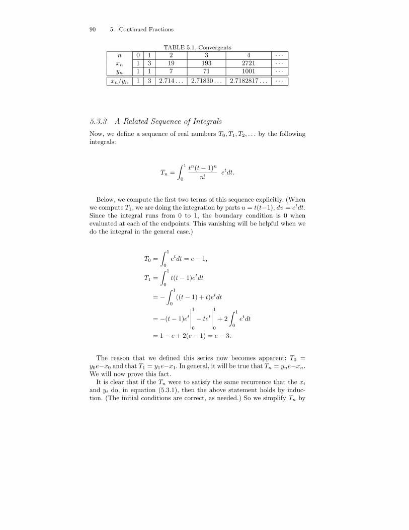
90 5. Continued Fractions
TABLE 5.1. Convergents
n 0 1 2 3 4 · · ·xn 1 3 19 193 2721 · · ·yn 1 1 7 71 1001 · · ·
xn/yn 1 3 2.714 . . . 2.71830 . . . 2.7182817 . . . · · ·
5.3.3 A Related Sequence of Integrals
Now, we define a sequence of real numbers T0, T1, T2, . . . by the followingintegrals:
Tn =
∫ 1
0
tn(t − 1)n
n!etdt.
Below, we compute the first two terms of this sequence explicitly. (Whenwe compute T1, we are doing the integration by parts u = t(t−1), dv = etdt.Since the integral runs from 0 to 1, the boundary condition is 0 whenevaluated at each of the endpoints. This vanishing will be helpful when wedo the integral in the general case.)
T0 =
∫ 1
0
etdt = e − 1,
T1 =
∫ 1
0
t(t − 1)etdt
= −∫ 1
0
((t − 1) + t)etdt
= −(t − 1)et
∣
∣
∣
∣
∣
1
0
− tet
∣
∣
∣
∣
∣
1
0
+ 2
∫ 1
0
etdt
= 1 − e + 2(e − 1) = e − 3.
The reason that we defined this series now becomes apparent: T0 =y0e−x0 and that T1 = y1e−x1. In general, it will be true that Tn = yne−xn.We will now prove this fact.
It is clear that if the Tn were to satisfy the same recurrence that the xi
and yi do, in equation (5.3.1), then the above statement holds by induc-tion. (The initial conditions are correct, as needed.) So we simplify Tn by
5.4 Quadratic Irrationals 91
integrating by parts twice in succession:
Tn =
∫ 1
0
tn(t − 1)n
n!etdt
= −∫ 1
0
tn−1(t − 1)n + tn(t − 1)n−1
(n − 1)!etdt
=
∫ 1
0
( tn−2(t − 1)n
(n − 2)!+ n
tn−1(t − 1)n−1
(n − 1)!
+ ntn−1(t − 1)n−1
(n − 1)!+
tn(t − 1)n−2
(n − 2)!
)
etdt
= 2nTn−1 +
∫ 1
0
tn−2(t − 1)n−2
n − 2!(2t2 − 2t + 1) etdt
= 2nTn−1 + 2
∫ 1
0
tn−1(t − 1)n−1
n − 2!etdt +
∫ 1
0
tn−2(t − 1)n−2
n − 2!etdt
= 2nTn−1 + 2(n − 1)Tn−1 + Tn−2
= 2(2n − 1)Tn−1 + Tn−2,
which is the desired recurrence.Therefore Tn = yne − xn. To conclude the proof, we consider the limit
as n approaches infinity:
limn→∞
∫ 1
0
tn(t − 1)n
n!etdt = 0,
by inspection, and therefore
limn→∞
xn
yn= lim
n→∞(e − Tn
yn) = e.
Therefore, the ratio xn/yn approaches e, and the continued fraction expan-sion [2, 1, 2, 1, 1, 4, 1, 1, . . .] does in fact converge to e.
5.3.4 Extensions of the Argument
The method of proof of this section generalizes to show that the continuedfraction expansion of e1/n is
[1, (n − 1), 1, 1, (3n − 1), 1, 1, (5n − 1), 1, 1, (7n − 1), . . .]
for all n ∈ N (see Exercise 5.6).
5.4 Quadratic Irrationals
The main result of this section is that the continued fraction expansion ofa number is eventually repeating if and only if the number is a quadratic
92 5. Continued Fractions
irrational. This can be viewed as an analogue for continued fractions ofthe familiar fact that the decimal expansion of x is eventually repeating ifand only if x is rational. The proof that continued fractions of quadraticirrationals eventually repeats is surprisingly difficult and involves an inter-esting finiteness argument. Section 5.4.2 emphasizes our striking ignoranceabout continued fractions of real roots of irreducible polynomials over Qof degree bigger than 2.
Definition 5.4.1 (Quadratic Irrational). A real number α ∈ R is aquadratic irrational if it is irrational and satisfies a quadratic polynomialwith coefficients in Q.
Thus, e.g., (1 +√
5)/2 is a quadratic irrational. Recall that
1 +√
5
2= [1, 1, 1, . . .].
The continued fraction of√
2 is [1, 2, 2, 2, 2, 2, . . .], and the continued frac-tion of
√389 is
[19, 1, 2, 1, 1, 1, 1, 2, 1, 38, 1, 2, 1, 1, 1, 1, 2, 1, 38, . . .].
Does the [1, 2, 1, 1, 1, 1, 2, 1, 38] pattern repeat over and over again?
5.4.1 Periodic Continued Fractions
Definition 5.4.2 (Periodic Continued Fraction). A periodic continuedfraction is a continued fraction [a0, a1, . . . , an, . . .] such that
an = an+h
for some fixed positive integer h and all sufficiently large n. We call theminimal such h the period of the continued fraction.
Example 5.4.3. Consider the periodic continued fraction [1, 2, 1, 2, . . .] =[1, 2]. What does it converge to? We have
[1, 2] = 1 +1
2 +1
1 +1
2 +1
1 + · · ·
,
so if α = [1, 2] then
α = 1 +1
2 +1
α
= 1 +1
2α + 1
α
= 1 +α
2α + 1=
3α + 1
2α + 1.
5.4 Quadratic Irrationals 93
Thus 2α2 − 2α − 1 = 0, so
α =1 +
√3
2.
Theorem 5.4.4 (Periodic Characterization). An infinite simple con-tinued fraction is periodic if and only if it represents a quadratic irrational.
Proof. (=⇒) First suppose that
[a0, a1, . . . , an, an+1, . . . , an+h]
is a periodic continued fraction. Set α = [an+1, an+2, . . .]. Then
α = [an+1, . . . , an+h, α],
so by Proposition 5.1.4
α =αpn+h + pn+h−1
αqn+h + qn+h−1.
Here we use that α is the last partial quotient. Thus, α satisfies a quadraticequation with coefficients in Q. Computing as in Example 5.4.3 and ratio-nalizing the denominators, and using that the ai are all integers, showsthat
[a0, a1, . . .] = [a0, a1, . . . , an, α]
= a0 +1
a1 +1
a2 + · · · + 1
α
is of the form c + dα, with c, d ∈ Q, so [a0, a1, . . .] also satisfies a quadraticpolynomial over Q.
The continued fraction procedure applied to the value of an infinite sim-ple continued fraction yields that continued fraction back, so by Proposi-tion 5.2.11, α 6∈ Q because it is the value of an infinite continued fraction.
(⇐=) Suppose α ∈ R is an irrational number that satisfies a quadraticequation
aα2 + bα + c = 0 (5.4.1)
with a, b, c ∈ Z and a 6= 0. Let [a0, a1, . . .] be the continued fraction expan-sion of α. For each n, let
rn = [an, an+1, . . .],
soα = [a0, a1, . . . , an−1, rn].
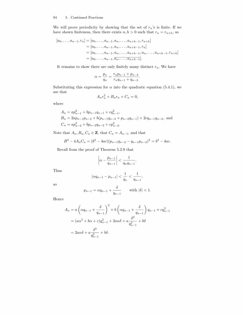
94 5. Continued Fractions
We will prove periodicity by showing that the set of rn’s is finite. If wehave shown finiteness, then there exists n, h > 0 such that rn = rn+h, so
[a0, . . . , an−1, rn] = [a0, . . . , an−1, an, . . . , an+h−1, rn+h]
= [a0, . . . , an−1, an, . . . , an+h−1, rn]
= [a0, . . . , an−1, an, . . . , an+h−1, an, . . . , an+h−1, rn+h]
= [a0, . . . , an−1, an, . . . , an+h−1].
It remains to show there are only finitely many distinct rn. We have
α =pn
qn=
rnpn−1 + pn−2
rnqn−1 + qn−2.
Substituting this expression for α into the quadratic equation (5.4.1), wesee that
Anr2n + Bnrn + Cn = 0,
where
An = ap2n−1 + bpn−1qn−1 + cq2
n−1,
Bn = 2apn−1pn−2 + b(pn−1qn−2 + pn−2qn−1) + 2cqn−1qn−2, and
Cn = ap2n−2 + bpn−2qn−2 + cp2
n−2.
Note that An, Bn, Cn ∈ Z, that Cn = An−1, and that
B2 − 4AnCn = (b2 − 4ac)(pn−1qn−2 − qn−1pn−2)2 = b2 − 4ac.
Recall from the proof of Theorem 5.2.9 that∣
∣
∣
∣
α − pn−1
qn−1
∣
∣
∣
∣
<1
qnqn−1.
Thus
|αqn−1 − pn−1| <1
qn<
1
qn−1,
so
pn−1 = αqn−1 +δ
qn−1with |δ| < 1.
Hence
An = a
(
αqn−1 +δ
qn−1
)2
+ b
(
αqn−1 +δ
qn−1
)
qn−1 + cq2n−1
= (aα2 + bα + c)q2n−1 + 2aαδ + a
δ2
q2n−1
+ bδ
= 2aαδ + aδ2
q2n−1
+ bδ.
5.4 Quadratic Irrationals 95
Thus
|An| =
∣
∣
∣
∣
2aαδ + aδ2
q2n−1
+ bδ
∣
∣
∣
∣
< 2|aα| + |a| + |b|.
Thus there are only finitely many possibilities for the integer An. Also,
|Cn| = |An−1| and |Bn| =√
b2 − 4(ac − AnCn),
so there are only finitely many triples (An, Bn, Cn), and hence only finitelymany possibilities for rn as n varies, which completes the proof. (The proofabove closely follows [HW79, Thm. 177, pg.144–145].)
5.4.2 Continued Fractions of Algebraic Numbers of Higher
Degree
Definition 5.4.5 (Algebraic Number). An algebraic number is a rootof a polynomial f ∈ Q[x].
Open Problem 5.4.6. Give a simple description of the complete contin-ued fractions expansion of the algebraic number 3
√2. It begins
[1, 3, 1, 5, 1, 1, 4, 1, 1, 8, 1, 14, 1, 10, 2, 1, 4, 12, 2, 3, 2, 1, 3, 4, 1, 1, 2, 14,
3, 12, 1, 15, 3, 1, 4, 534, 1, 1, 5, 1, 1, . . .]
The author does not see a pattern, and the 534 reduces his confidencethat he will. Lang and Trotter (see [LT72]) analyzed many terms of thecontinued fraction of 3
√2 statistically, and their work suggests that 3
√2 has
an “unusual” continued fraction; later work in [LT74] suggests that maybeit does not.
Khintchine (see [Khi63, pg. 59])
No properties of the representing continued fractions, analogousto those which have just been proved, are known for algebraicnumbers of higher degree [as of 1963]. [...] It is of interest topoint out that up till the present time no continued fractiondevelopment of an algebraic number of higher degree than thesecond is known [emphasis added]. It is not even known if sucha development has bounded elements. Generally speaking theproblems associated with the continued fraction expansion of al-gebraic numbers of degree higher than the second are extremelydifficult and virtually unstudied.
Richard Guy (see [Guy94, pg. 260])
Is there an algebraic number of degree greater than two whosesimple continued fraction has unbounded partial quotients? Doesevery such number have unbounded partial quotients?
96 5. Continued Fractions
Baum and Sweet [BS76] answered the analogue of Richard Guy’s ques-tion but with algebraic numbers replaced by elements of a field K otherthan Q. (The field K is F2((1/x)), the field of Laurent series in the variable1/x over the finite field with two elements. An element of K is a polyno-mial in x plus a formal power series in 1/x.) They found an α of degreethree over K whose continued fraction has all terms of bounded degree, andother elements of various degrees greater than 2 over K whose continuedfractions have terms of unbounded degree.
5.5 Recognizing Rational Numbers
Suppose that somehow you can compute approximations to some rationalnumber, and want to figure what the rational number probably is. Com-puting the approximation to high enough precision to find a period in thedecimal expansion is not a good approach, because the period can be huge(see below). A much better approach is to compute the simple continuedfraction of the approximation, and truncate it before a large partial quo-tient an, then compute the value of the truncated continued fraction. Thisresults in a rational number that has relatively small numerator and de-nominator, and is close to the approximation of the rational number, sincethe tail end of the continued fraction is at most 1/an.
We begin with a contrived example, which illustrates how to recognize arational number. Let
x = 9495/3847 = 2.46815700545879906420587470756433584611385 . . . .
The continued fraction of the truncation 2.468157005458799064 is
[2, 2, 7, 2, 1, 5, 1, 1, 1, 1, 1, 1, 328210621945, 2, 1, 1, 1, . . .]
We have
[2, 2, 7, 2, 1, 5, 1, 1, 1, 1, 1, 1] =9495
3847.
Notice that no repetition is evident in the digits of x given above, thoughwe know that the decimal expansion of x must be eventually periodic, sinceall decimal expansions of rational numbers are eventually periodic. In fact,the length of the period of the decimal expansion of 1/3847 is 3846, whichis the order of 10 modulo 3847 (see Exercise 5.7).
For a slightly less contrived application of this idea, suppose f(x) ∈ Z[x]is a polynomial with integer coefficients, and we know for some reason thatone root of f is a rational number. Then we can find that rational num-ber by using Newton’s method to approximate each root, and continuedfractions to decide whether each root is a rational number (we can substi-tute the value of the continued fraction approximation into f to see if it
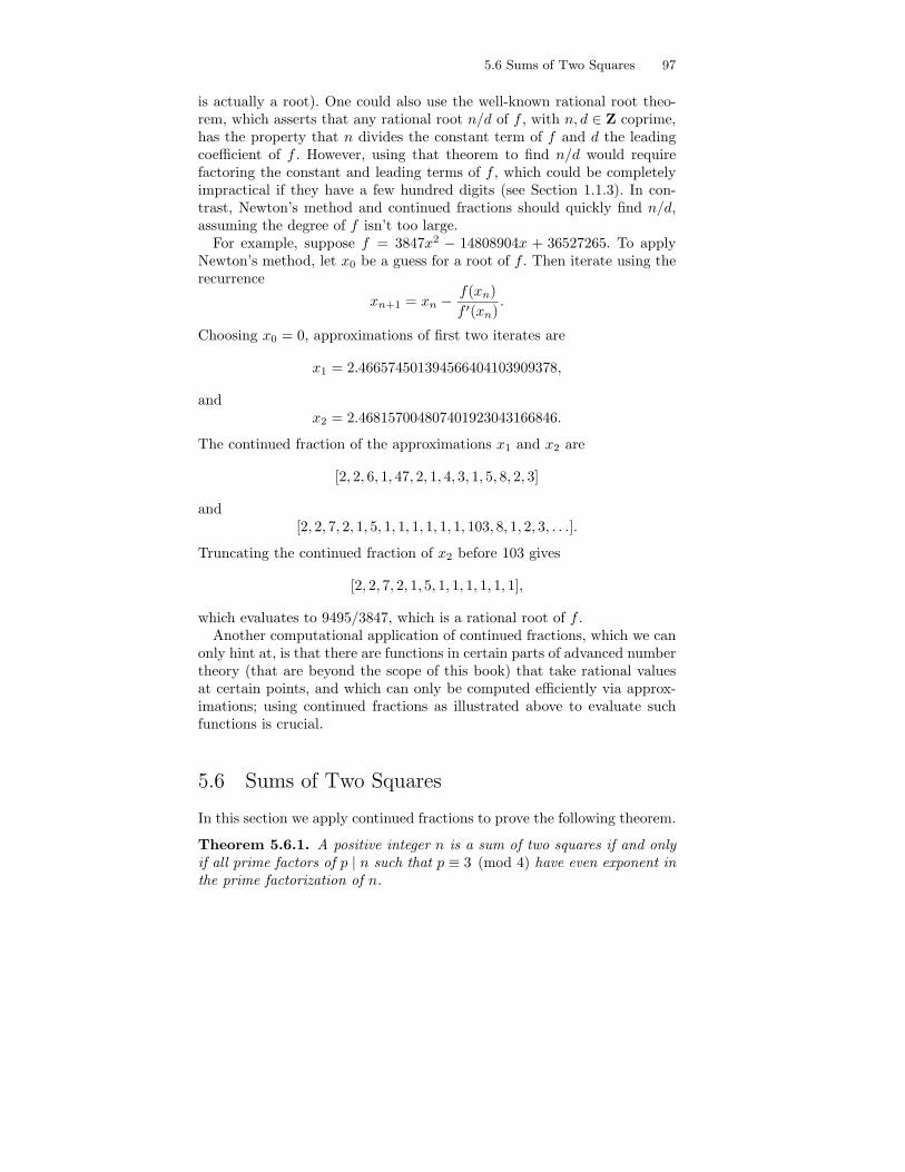
5.6 Sums of Two Squares 97
is actually a root). One could also use the well-known rational root theo-rem, which asserts that any rational root n/d of f , with n, d ∈ Z coprime,has the property that n divides the constant term of f and d the leadingcoefficient of f . However, using that theorem to find n/d would requirefactoring the constant and leading terms of f , which could be completelyimpractical if they have a few hundred digits (see Section 1.1.3). In con-trast, Newton’s method and continued fractions should quickly find n/d,assuming the degree of f isn’t too large.
For example, suppose f = 3847x2 − 14808904x + 36527265. To applyNewton’s method, let x0 be a guess for a root of f . Then iterate using therecurrence
xn+1 = xn − f(xn)
f ′(xn).
Choosing x0 = 0, approximations of first two iterates are
x1 = 2.466574501394566404103909378,
andx2 = 2.468157004807401923043166846.
The continued fraction of the approximations x1 and x2 are
[2, 2, 6, 1, 47, 2, 1, 4, 3, 1, 5, 8, 2, 3]
and[2, 2, 7, 2, 1, 5, 1, 1, 1, 1, 1, 1, 103, 8, 1, 2, 3, . . .].
Truncating the continued fraction of x2 before 103 gives
[2, 2, 7, 2, 1, 5, 1, 1, 1, 1, 1, 1],
which evaluates to 9495/3847, which is a rational root of f .Another computational application of continued fractions, which we can
only hint at, is that there are functions in certain parts of advanced numbertheory (that are beyond the scope of this book) that take rational valuesat certain points, and which can only be computed efficiently via approx-imations; using continued fractions as illustrated above to evaluate suchfunctions is crucial.
5.6 Sums of Two Squares
In this section we apply continued fractions to prove the following theorem.
Theorem 5.6.1. A positive integer n is a sum of two squares if and onlyif all prime factors of p | n such that p ≡ 3 (mod 4) have even exponent inthe prime factorization of n.
98 5. Continued Fractions
We first consider some examples. Notice that 5 = 12 + 22 is a sum oftwo squares, but 7 is not a sum of two squares. Since 2001 is divisibleby 3 (because 2 + 1), but not by 9 (since 2 + 1 is not), Theorem 5.6.1implies that 2001 is not a sum of two squares. The theorem also impliesthat 2 · 34 · 5 · 72 · 13 is a sum of two squares.
Definition 5.6.2 (Primitive). A representation n = x2 + y2 is primitiveif x and y are coprime.
Lemma 5.6.3. If n is divisible by a prime p ≡ 3 (mod 4), then n has noprimitive representations.
Proof. Suppose n has a primitive representation, n = x2 + y2, and let p beany prime factor of n. Then
p | x2 + y2 and gcd(x, y) = 1,
so p ∤ x and p ∤ y. Since Z/pZ is a field we may divide by y2 in the equationx2 + y2 ≡ 0 (mod p) to see that (x/y)2 ≡ −1 (mod p). Thus the quadratic
residue symbol(
−1p
)
equals +1. However, by Proposition 4.2.1,
(−1
p
)
= (−1)(p−1)/2
so(
−1p
)
= 1 if and only if (p−1)/2 is even, which is to say p ≡ 1 (mod 4).
Proof of Theorem 5.6.1 (=⇒). Suppose that p ≡ 3 (mod 4) is a prime,that pr | n but pr+1 ∤ n with r odd, and that n = x2 + y2. Letting d =gcd(x, y), we have
x = dx′, y = dy′, and n = d2n′
with gcd(x′, y′) = 1 and
(x′)2 + (y′)2 = n′.
Because r is odd, p | n′, so Lemma 5.6.3 implies that gcd(x′, y′) > 1, acontradiction.
To prepare for our proof of (⇐=), we reduce the problem to the casewhen n is prime. Write n = n2
1n2 where n2 has no prime factors p ≡ 3(mod 4). It suffices to show that n2 is a sum of two squares, since
(x21 + y2
1)(x22 + y2
2) = (x1x2 − y1y2)2 + (x1y2 + x2y1)
2, (5.6.1)
so a product of two numbers that are sums of two squares is also a sum oftwo squares. Since 2 = 12 + 12 is a sum of two squares, it suffices to showthat any prime p ≡ 1 (mod 4) is a sum of two squares.
5.6 Sums of Two Squares 99
Lemma 5.6.4. If x ∈ R and n ∈ N, then there is a fractiona
bin lowest
terms such that 0 < b ≤ n and∣
∣
∣x − a
b
∣
∣
∣≤ 1
b(n + 1).
Proof. Consider the continued fraction [a0, a1, . . .] of x. By Corollary 5.2.10,for each m
∣
∣
∣
∣
x − pm
qm
∣
∣
∣
∣
<1
qm · qm+1.
Since qm+1 ≥ qm + 1 and q0 = 1, either there exists an m such thatqm ≤ n < qm+1, or the continued fraction expansion of x is finite and nis larger than the denominator of the rational number x, in which case wetake a
b = x and are done. In the first case,
∣
∣
∣
∣
x − pm
qm
∣
∣
∣
∣
<1
qm · qm+1≤ 1
qm · (n + 1),
soa
b=
pm
qmsatisfies the conclusion of the lemma.
Proof of Theorem 5.6.1 (⇐=). As discussed above, it suffices to prove thatany prime p ≡ 1 (mod 4) is a sum of two squares. Since p ≡ 1 (mod 4),
(−1)(p−1)/2 = 1,
so Proposition 4.2.1 implies that −1 is a square modulo p; i.e., there ex-ists r ∈ Z such that r2 ≡ −1 (mod p). Lemma 5.6.4, with n = ⌊√p⌋ andx = − r
p , implies that there are integers a, b such that 0 < b <√
p and
∣
∣
∣
∣
−r
p− a
b
∣
∣
∣
∣
≤ 1
b(n + 1)<
1
b√
p.
Letting c = rb + pa, we have that
|c| <pb
b√
p=
p√p
=√
p
so0 < b2 + c2 < 2p.
But c ≡ rb (mod p), so
b2 + c2 ≡ b2 + r2b2 ≡ b2(1 + r2) ≡ 0 (mod p).
Thus b2 + c2 = p.
Remark 5.6.5. Our proof of Theorem 5.6.1 leads to an efficient algorithmto compute a representation of any p ≡ 1 (mod 4) as a sum of two squares.See Listing 7.5.5 for an implementation.
100 5. Continued Fractions
5.7 Exercises
5.1 If cn = pn/qn is the nth convergent of [a0, a1, . . . , an] and a0 > 0,show that
[an, an−1, . . . , a1, a0] =pn
pn−1
and[an, an−1, . . . , a2, a1] =
qn
qn−1.
(Hint: In the first case, notice thatpn
pn−1= an +
pn−2
pn−1= an +
1pn−1
pn−2
.)
5.2 Show that every nonzero rational number can be represented in ex-actly two ways be a finite simple continued fraction. (For example, 2can be represented by [1, 1] and [2], and 1/3 by [0, 3] and [0, 2, 1].)
5.3 Evaluate the infinite continued fraction [2, 1, 2, 1].
5.4 Determine the infinite continued fraction of 1+√
132 .
5.5 Let a0 ∈ R and a1, . . . , an and b be positive real numbers. Prove that
[a0, a1, . . . , an + b] < [a0, a1, . . . , an]
if and only if n is odd.
5.6 (*) Extend the method presented in the text to show that the con-tinued fraction expansion of e1/k is
[1, (k − 1), 1, 1, (3k − 1), 1, 1, (5k − 1), 1, 1, (7k − 1), . . .]
for all k ∈ N.
(a) Compute p0, p3, q0, and q3 for the above continued fraction.Your answers should be in terms of k.
(b) Condense three steps of the recurrence for the numerators anddenominators of the above continued fraction. That is, producea simple recurrence for r3n in terms of r3n−3 and r3n−6 whosecoefficients are polynomials in n and k.
(c) Define a sequence of real numbers by
Tn(k) =1
kn
∫ 1/k
0
(kt)n(kt − 1)n
n!etdt.
i. Compute T0(k), and verify that it equals q0e1/k − p0.
ii. Compute T1(k), and verify that it equals q3e1/k − p3.
5.7 Exercises 101
iii. Integrate Tn(k) by parts twice in succession, as in Sec-tion 5.3, and verify that Tn(k), Tn−1(k), and Tn−2(k) satisfythe recurrence produced in part 6b, for n ≥ 2.
(d) Conclude that the continued fraction
[1, (k − 1), 1, 1, (3k − 1), 1, 1, (5k − 1), 1, 1, (7k − 1), . . .]
represents e1/k.
5.7 Let d be an integer that is coprime to 10. Prove that the decimalexpansion of 1
d has period equal to the order of 10 modulo d. (Hint:For every positive integer r, we have 1
1−10r =∑
n≥1 10−rn.)
5.8 Find a positive integer that has at least three different representationsas the sum of two squares, disregarding signs and the order of thesummands.
5.9 Show that if a natural number n is the sum of two two rational squaresit is also the sum of two integer squares.
5.10 (*) Let p be an odd prime. Show that p ≡ 1, 3 (mod 8) if and onlyif p can be written as p = x2+2y2 for some choice of integers x and y.
5.11 Prove that of any four consecutive integers, at least one is not repre-sentable as a sum of two squares.

102 5. Continued Fractions
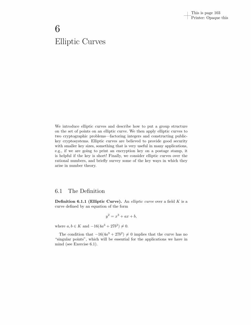
This is page 103Printer: Opaque this
6Elliptic Curves
We introduce elliptic curves and describe how to put a group structureon the set of points on an elliptic curve. We then apply elliptic curves totwo cryptographic problems—factoring integers and constructing public-key cryptosystems. Elliptic curves are believed to provide good securitywith smaller key sizes, something that is very useful in many applications,e.g., if we are going to print an encryption key on a postage stamp, itis helpful if the key is short! Finally, we consider elliptic curves over therational numbers, and briefly survey some of the key ways in which theyarise in number theory.
6.1 The Definition
Definition 6.1.1 (Elliptic Curve). An elliptic curve over a field K is acurve defined by an equation of the form
y2 = x3 + ax + b,
where a, b ∈ K and −16(4a3 + 27b2) 6= 0.
The condition that −16(4a3 + 27b2) 6= 0 implies that the curve has no“singular points”, which will be essential for the applications we have inmind (see Exercise 6.1).
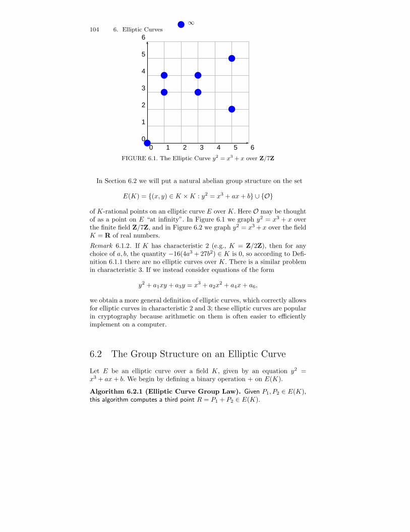
104 6. Elliptic Curves
0 1 2 3 4 5 60
1
2
3
4
5
6
∞
FIGURE 6.1. The Elliptic Curve y2 = x3 + x over Z/7Z
In Section 6.2 we will put a natural abelian group structure on the set
E(K) = {(x, y) ∈ K × K : y2 = x3 + ax + b} ∪ {O}
of K-rational points on an elliptic curve E over K. Here O may be thoughtof as a point on E “at infinity”. In Figure 6.1 we graph y2 = x3 + x overthe finite field Z/7Z, and in Figure 6.2 we graph y2 = x3 + x over the fieldK = R of real numbers.
Remark 6.1.2. If K has characteristic 2 (e.g., K = Z/2Z), then for anychoice of a, b, the quantity −16(4a3 + 27b2) ∈ K is 0, so according to Defi-nition 6.1.1 there are no elliptic curves over K. There is a similar problemin characteristic 3. If we instead consider equations of the form
y2 + a1xy + a3y = x3 + a2x2 + a4x + a6,
we obtain a more general definition of elliptic curves, which correctly allowsfor elliptic curves in characteristic 2 and 3; these elliptic curves are popularin cryptography because arithmetic on them is often easier to efficientlyimplement on a computer.
6.2 The Group Structure on an Elliptic Curve
Let E be an elliptic curve over a field K, given by an equation y2 =x3 + ax + b. We begin by defining a binary operation + on E(K).
Algorithm 6.2.1 (Elliptic Curve Group Law). Given P1, P2 ∈ E(K),this algorithm computes a third point R = P1 + P2 ∈ E(K).
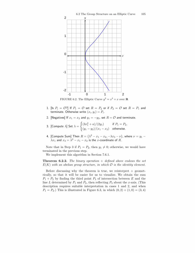
6.2 The Group Structure on an Elliptic Curve 105
-1 0 1 2-2
-1
0
1
2
x
y
FIGURE 6.2. The Elliptic Curve y2 = x3 + x over R
1. [Is Pi = O?] If P1 = O set R = P2 or if P2 = O set R = P1 andterminate. Otherwise write (xi, yi) = Pi.
2. [Negatives] If x1 = x2 and y1 = −y2, set R = O and terminate.
3. [Compute λ] Set λ =
{
(3x21 + a)/(2y1) if P1 = P2,
(y1 − y2)/(x1 − x2) otherwise.
4. [Compute Sum] Then R =(
λ2 − x1 − x2,−λx3 − ν)
, where ν = y1 −λx1 and x3 = λ2 − x1 − x2 is the x-coordinate of R.
Note that in Step 3 if P1 = P2, then y1 6= 0; otherwise, we would haveterminated in the previous step.
We implement this algorithm in Section 7.6.1.
Theorem 6.2.2. The binary operation + defined above endows the setE(K) with an abelian group structure, in which O is the identity element.
Before discussing why the theorem is true, we reinterpret + geomet-rically, so that it will be easier for us to visualize. We obtain the sumP1 + P2 by finding the third point P3 of intersection between E and theline L determined by P1 and P2, then reflecting P3 about the x-axis. (Thisdescription requires suitable interpretation in cases 1 and 2, and whenP1 = P2.) This is illustrated in Figure 6.3, in which (0, 2) + (1, 0) = (3, 4)

106 6. Elliptic Curves
on y2 = x3 − 5x + 4. To further clarify this geometric interpretation, weprove the following proposition.
Proposition 6.2.3 (Geometric group law). Suppose Pi = (xi, yi), i =1, 2 are distinct point on an elliptic curve y2 = x3+ax+b, and that x1 6= x2.Let L be the unique line through P1 and P2. Then L intersects the graphof E at exactly one other point
Q =(
λ2 − x1 − x2, λx3 + ν)
,
where λ = (y1 − y2)/(x1 − x2) and ν = y1 − λx1.
Proof. The line L through P1, P2 is y = y1 + (x − x1)λ. Substituting thisinto y2 = x3 + ax + b we get
(y1 + (x − x1)λ)2 = x3 + ax + b.
Simplifying we get f(x) = x3−λ2x2+· · · = 0, where we omit the coefficientsof x and the constant term since they will not be needed. Since P1 and P2
are in L∩E, the polynomial f has x1 and x2 as roots. By Proposition 2.5.2,the polynomial f can have at most three roots. Writing f =
∏
(x−xi) andequating terms, we see that x1 + x2 + x3 = λ2. Thus x3 = λ2 − x1 − x2, asclaimed. Also, from the equation for L we see that y3 = y1 + (x3 − x1)λ =λx3 + ν, which completes the proof.
To prove Theorem 6.2.2 means to show that + satisfies the three axiomsof an abelian group with O as identity element: existence of inverses, com-mutativity, and associativity. The existence of inverses follows immediatelyfrom the definition, since (x, y)+ (x,−y) = O. Commutativity is also clearfrom the definition of group law, since in parts 1–3, the recipe is unchangedif we swap P1 and P2; in part 4 swapping P1 and P2 does not change theline determined by P1 and P2, so by Proposition 6.2.3 it does not changethe sum P1 + P2.
It is more difficult to prove that + satisfies the associative axiom, i.e.,that (P1 + P2) + P3 = P1 + (P2 + P3). This fact can be understood from atleast three points of view. One is to reinterpret the group law geometrically(extending Proposition 6.2.3 to all cases), and thus transfer the problemto a question in plane geometry. This approach is beautifully explainedwith exactly the right level of detail in [ST92, §I.2]. Another approach is touse the formulas that define + to reduce associativity to checking specificalgebraic identities; this is something that would be extremely tedious to doby hand, but can be done using a computer (also tedious). A third approach(see e.g. [Sil86] or [Har77]) is to develop a general theory of “divisors onalgebraic curves”, from which associativity of the group law falls out as anatural corollary. The third approach is the best, because it opens up manynew vistas; however we will not pursue it further because it is beyond thescope of this book.
6.3 Integer Factorization Using Elliptic Curves 107
-3 -2 -1 0 1 2 3 4-5
-4
-3
-2
-1
0
1
2
3
4
5
x
y
L
L′
(1, 0)
(0, 2)
(3,−4)
(3, 4)
FIGURE 6.3. The Group Law: (1, 0) + (0, 2) = (3, 4) on y2 = x3− 5x + 4
6.3 Integer Factorization Using Elliptic Curves
In 1987, Hendrik Lenstra published the landmark paper [Len87] that intro-duces and analyzes the Elliptic Curve Method (ECM), which is a powerfulalgorithm for factoring integers using elliptic curves. Lenstra’s method isalso described in [ST92, §IV.4], [Dav99, §VIII.5], and [Coh93, §10.3].
Lenstra’s algorithm is well suited for finding“medium sized” factors of an integer N , whichtoday means 10 to 20 decimal digits. The ECMmethod is not directly used for factoring RSA chal-lenge numbers (see Section 1.1.3), but it is used onauxiliary numbers as a crucial step in the “numberfield sieve”, which is the best known algorithm forhunting for such factorizations. Also, implementa-tion of ECM typically requires little memory. Lenstra
6.3.1 Pollard’s (p − 1)-Method
Lenstra’s discovery of ECM was inspired by Pollard’s (p−1)-method, whichwe describe in this section.

108 6. Elliptic Curves
Definition 6.3.1 (Power smooth). Let B be a positive integer. If n isa positive integer with prime factorization n =
∏
pei
i , then n is B-powersmooth if pei
i ≤ B for all i.
Thus 30 = 2 · 3 · 5 is B power smooth for B = 5, 7, but 150 = 2 · 3 · 52 isnot 5-power smooth (it is B = 25-power smooth).
We will use the following algorithm in both the Pollard p−1 and ellipticcurve factorization methods.
Algorithm 6.3.2 (Least Common Multiple of First B Integers).Given a positive integer B, this algorithm computes the least common multipleof the positive integers up to B.
1. [Sieve] Using, e.g., the Sieve of Eratosthenes (Algorithm 1.2.3), computea list P of all primes p ≤ B.
2. [Multiply] Compute and output the product∏
p∈P ⌊logp(B)⌋.
Proof. Let m = lcm(1, 2, . . . , B). Then
ordp(m) = max({ordp(n) : 1 ≤ n ≤ B}) = ordp(pr),
where pr is the largest power of p that satisfies pr ≤ B. Since pr ≤ B <pr+1, we have r = ⌊logp(B)⌋.
We implement Algorithm 6.3.2 in Section 7.6.2.Let N be a positive integer that we wish to factor. We use the Pollard
(p − 1)-method to look for a nontrivial factor of N as follows. First wechoose a positive integer B, usually with at most six digits. Suppose thatthere is a prime divisor p of N such that p− 1 is B-power smooth. We tryto find p using the following strategy. If a > 1 is an integer not divisibleby p then by Theorem 2.1.12,
ap−1 ≡ 1 (mod p).
Let m = lcm(1, 2, 3, . . . , B), and observe that our assumption that p− 1 isB-power smooth implies that p − 1 | m, so
am ≡ 1 (mod p).
Thusp | gcd(am − 1, N) > 1.
If gcd(am−1, N) < N also then gcd(am−1, N) is a nontrivial factor of N . Ifgcd(am − 1, N) = N , then am ≡ 1 (mod qr) for every prime power divisorqr of N . In this case, repeat the above steps but with a smaller choice of Bor possibly a different choice of a. Also, it is a good idea to check fromthe start whether or not N is not a perfect power Mr, and if so replace Nby M . We formalize the algorithm as follows:
6.3 Integer Factorization Using Elliptic Curves 109
Algorithm 6.3.3 (Pollard p − 1 Method). Given a positive integer Nand a bound B, this algorithm attempts to find a nontrivial factor m of N .(Each prime p | m is likely to have the property that p−1 is B-power smooth.)
1. [Compute lcm] Use Algorithm 6.3.2 to compute m = lcm(1, 2, . . . , B).
2. [Initialize] Set a = 2.
3. [Power and gcd] Compute x = am − 1 (mod N) and g = gcd(x,N).
4. [Finished?] If g 6= 1 or N , output g and terminate.
5. [Try Again?] If a < 10 (say), replace a by a + 1 and go to step 3.Otherwise terminate.
We implement Algorithm 6.3.3 in Section 7.6.2.For fixed B, Algorithm 6.3.3 often splits N when N is divisible by a
prime p such that p−1 is B-power smooth. Approximately 15% of primes pin the interval from 1015 and 1015 +10000 are such that p−1 is 106 power-smooth, so the Pollard method with B = 106 already fails nearly 85% ofthe time at finding 15-digit primes in this range (see also Exercise 7.14).We will not analyze Pollard’s method further, since it was mentioned hereonly to set the stage for the elliptic curve factorization method.
The following examples illustrate the Pollard (p − 1)-method.
Example 6.3.4. In this example, Pollard works perfectly. Let N = 5917.We try to use the Pollard p − 1 method with B = 5 to split N . We havem = lcm(1, 2, 3, 4, 5) = 60; taking a = 2 we have
260 − 1 ≡ 3416 (mod 5917)
and
gcd(260 − 1, 5917) = gcd(3416, 5917) = 61,
so 61 is a factor of 5917.
Example 6.3.5. In this example, we replace B by larger integer. Let N =779167. With B = 5 and a = 2 we have
260 − 1 ≡ 710980 (mod 779167),
and gcd(260 − 1, 779167) = 1. With B = 15, we have
m = lcm(1, 2, . . . , 15) = 360360,
2360360 − 1 ≡ 584876 (mod 779167),
and
gcd(2360360 − 1, N) = 2003,
so 2003 is a nontrivial factor of 779167.
110 6. Elliptic Curves
Example 6.3.6. In this example, we replace B by a smaller integer. LetN = 4331. Suppose B = 7, so m = lcm(1, 2, . . . , 7) = 420,
2420 − 1 ≡ 0 (mod 4331),
and gcd(2420 − 1, 4331) = 4331, so we do not obtain a factor of 4331. If wereplace B by 5, Pollard’s method works:
260 − 1 ≡ 1464 (mod 4331),
and gcd(260 − 1, 4331) = 61, so we split 4331.
Example 6.3.7. In this example, a = 2 does not work, but a = 3 does. LetN = 187. Suppose B = 15, so m = lcm(1, 2, . . . , 15) = 360360,
2360360 − 1 ≡ 0 (mod 187),
and gcd(2360360 − 1, 187) = 187, so we do not obtain a factor of 187. If wereplace a = 2 by a = 3, then Pollard’s method works:
3360360 − 1 ≡ 66 (mod 187),
and gcd(3360360 − 1, 187) = 11. Thus 187 = 11 · 17.
6.3.2 Motivation for the Elliptic Curve Method
Fix a positive integer B. If N = pq with p and q prime and p− 1 and q− 1are not B-power smooth, then the Pollard (p − 1)-method is unlikely towork. For example, let B = 20 and suppose that N = 59 ·101 = 5959. Notethat neither 59 − 1 = 2 · 29 nor 101 − 1 = 4 · 25 is B-power smooth. Withm = lcm(1, 2, 3, . . . , 20) = 232792560, we have
2m − 1 ≡ 5944 (mod N),
and gcd(2m − 1, N) = 1, so we do not find a factor of N .As remarked above, the problem is that p−1 is not 20-power smooth for
either p = 59 or p = 101. However, notice that p − 2 = 3 · 19 is 20-powersmooth. Lenstra’s ECM replaces (Z/pZ)∗, which has order p − 1, by thegroup of points on an elliptic curve E over Z/pZ. It is a theorem that
#E(Z/pZ) = p + 1 ± s
for some nonnegative integer s < 2√
p (see e.g., [Sil86, §V.1] for a proof).(Also every value of s subject to this bound occurs, as one can see using“complex multiplication theory”.) For example, if E is the elliptic curve
y2 = x3 + x + 54
over Z/59Z then by enumerating points one sees that E(Z/59Z) is cyclicof order 57. The set of numbers 59 + 1± s for s ≤ 15 contains 14 numbersthat are B-power smooth for B = 20 (see Exercise 7.14). Thus workingwith an elliptic curve gives us more flexibility. For example, 60 = 59+1+0is 5-power smooth and 70 = 59 + 1 + 10 is 7-power smooth.

6.3 Integer Factorization Using Elliptic Curves 111
FIGURE 6.4. Hendrik Lenstra
6.3.3 Lenstra’s Elliptic Curve Factorization Method
Algorithm 6.3.8 (Elliptic Curve Factorization Method). Given apositive integer N and a bound B, this algorithm attempts to find a nontrivialfactor m of N . Carry out the following steps:
1. [Compute lcm] Use Algorithm 6.3.2 to compute m = lcm(1, 2, . . . , B).
2. [Choose Random Elliptic Curve] Choose a random a ∈ Z/NZ such that4a3 + 27 ∈ (Z/NZ)∗. Then P = (0, 1) is a point on the elliptic curvey2 = x3 + ax + 1 over Z/NZ.
3. [Compute Multiple] Attempt to compute mP using an elliptic curveanalogue of Algorithm 2.3.7. If at some point we cannot compute a sumof points because some denominator in step 3 of Algorithm 6.2.1 is notcoprime to N , we compute the gcd of this denominator with N . If thisgcd is a nontrivial divisor, output it. If every denominator is coprimeto N , output “Fail”.
We implement Algorithm 6.3.8 in Section 7.6.2.If Algorithm 6.3.8 fails for one random elliptic curve, there is an option
that is unavailable with Pollard’s (p−1)-method—we may repeat the abovealgorithm with a different elliptic curve. With Pollard’s method we alwayswork with the group (Z/NZ)∗, but here we can try many groups E(Z/NZ)for many curves E. As mentioned above, the number of points on E overZ/pZ is of the form p + 1 − t for some t with |t| < 2
√p; Algorithm 6.3.8
thus has a chance if p+1− t is B-power-smooth for some t with |t| < 2√
p.
6.3.4 Examples
For simplicity, we use an elliptic curve of the form
y2 = x3 + ax + 1,
which has the point P = (0, 1) already on it.We factor N = 5959 using the elliptic curve method. Let
m = lcm(1, 2, . . . , 20) = 232792560 = 11011110000000100001111100002,
112 6. Elliptic Curves
where x2 means x is written in binary. First we choose a = 1201 at randomand consider y2 = x3 + 1201x + 1 over Z/5959Z. Using the formula forP+P from Algorithm 6.2.1 implemented on a computer (see Section 7.6) wecompute 2i ·P = 2i · (0, 1) for i ∈ B = {4, 5, 6, 7, 8, 13, 21, 22, 23, 24, 26, 27}.Then
∑
i∈B 2iP = mP . It turns out that during no step of this computationdoes a number not coprime to 5959 appear in any denominator, so we donot split N using a = 1201. Next we try a = 389 and at some stage inthe computation we add P = (2051, 5273) and Q = (637, 1292). Whencomputing the group law explicitly we try to compute λ = (y1 − y2)/(x1 −x2) in (Z/5959Z)∗, but fail since x1−x2 = 1414 and gcd(1414, 5959) = 101.We thus find a nontrivial factor 101 of 5959.
For bigger examples and an implementation of the algorithm, see Sec-tion 7.6.2.
6.3.5 A Heuristic Explanation
Let N be a positive integer and for simplicity of exposition assume thatN = p1 · · · pr with the pi distinct primes. It follows from Lemma 2.2.5 thatthere is a natural isomorphism
f : (Z/NZ)∗ −→ (Z/p1Z)∗ × · · · × (Z/prZ)∗.
When using Pollard’s method, we choose an a ∈ (Z/NZ)∗, compute am,then compute gcd(am−1, N). This gcd is divisible exactly by the primes pi
such that am ≡ 1 (mod pi). To reinterpret Pollard’s method using theabove isomorphism, let (a1, . . . , ar) = f(a). Then (am
1 , . . . , amr ) = f(am),
and the pi that divide gcd(am − 1, N) are exactly the pi such that ami = 1.
By Theorem 2.1.12, these pi include the primes pj such that pj − 1 isB-power smooth, where m = lcm(1, . . . ,m).
We will not define E(Z/NZ) when N is composite, since this is notneeded for the algorithm (where we assume that N is prime and hope fora contradiction). However, for the remainder of this paragraph, we pretendthat E(Z/NZ) is meaningful and describe a heuristic connection betweenLenstra and Pollard’s methods. The significant difference between Pollard’smethod and the elliptic curve method is that the isomorphism f is replacedby an isomorphism (in quotes)
“g : E(Z/NZ) → E(Z/p1Z) × · · · × E(Z/prZ)”
where E is y2 = x3 + ax + 1, and the a of Pollard’s method is replaced byP = (0, 1). We put the isomorphism in quotes to emphasize that we havenot defined E(Z/NZ). When carrying out the elliptic curve factorizationalgorithm, we attempt to compute mP and if some components of f(Q)are O, for some point Q that appears during the computation, but othersare nonzero, we find a nontrivial factor of N .
6.4 Elliptic Curve Cryptography 113
6.4 Elliptic Curve Cryptography
In this section we discuss an analogue of Diffie-Hellman that uses an ellipticcurve instead of (Z/pZ)∗. The idea to use elliptic curves in cryptographywas independently proposed by Neil Koblitz and Victor Miller in the mid1980s. We then discuss the ElGamal elliptic curve cryptosystem.
6.4.1 Elliptic Curve Analogues of Diffie-Hellman
The Diffie-Hellman key exchange from Section 3.1 works well on an ellipticcurve with no serious modification. Michael and Nikita agree on a secretkey as follows:
1. Michael and Nikita agree on a prime p, an elliptic curve E over Z/pZ,and a point P ∈ E(Z/pZ).
2. Michael secretly chooses a random m and sends mP .
3. Nikita secretly chooses a random n and sends nP .
4. The secret key is nmP , which both Michael and Nikita can compute.
Presumably, an adversary can not compute nmP without solving the dis-crete logarithm problem (see Problem 3.1.2 and Section 6.4.3 below) inE(Z/pZ). For well-chosen E, P , and p experience suggests that the discretelogarithm problem in E(Z/pZ) is much more difficult than the discrete log-arithm problem in (Z/pZ)∗ (see Section 6.4.3 for more on the elliptic curvediscrete log problem).
6.4.2 The ElGamal Cryptosystem and Digital Rights
Management
This section is about the ElGamal cryptosystem, which works well onan elliptic curves. This section draws on a paper by an actual computerhacker named Beale Screamer who cracked a “Digital Rights Management”(DRM) system.
The elliptic curve used in the DRM is an elliptic curve over the finitefield k = Z/pZ, where
p = 785963102379428822376694789446897396207498568951.
In base 16 the number p is
89ABCDEF012345672718281831415926141424F7,
which includes counting in hexadecimal, and digits of e, π, and√
2. Theelliptic curve E is
y2 = x3 + 317689081251325503476317476413827693272746955927x
+ 79052896607878758718120572025718535432100651934.
114 6. Elliptic Curves
We have
#E(k) = 785963102379428822376693024881714957612686157429,
and the group E(k) is cyclic with generator
B = (771507216262649826170648268565579889907769254176,
390157510246556628525279459266514995562533196655).
Our heroes Nikita and Michael share digital music when they are notout fighting terrorists. When Nikita installed the DRM software on hercomputer, it generated a private key
n = 670805031139910513517527207693060456300217054473,
which it hides in bits and pieces of files. In order for Nikita to play JunoReactor’s latest hit juno, her web browser contacts a web site that sellsmusic. After Nikita sends her credit card number, that web site allowsNikita to download a license file that allows her audio player to unlock andplay juno.
As we will see below, the license file was created using the ElGamalpublic-key cryptosystem in the group E(k). Nikita can now use her licensefile to unlock juno. However, when she shares both juno and the licensefile with Michael, he is frustrated because even with the license his com-puter still does not play juno. This is because Michael’s computer does notknow Nikita’s computer’s private key (the integer n above), so Michael’scomputer can not decrypt the license file.
We now describe the ElGamal cryptosystem, which lends itself well toimplementation in the group E(Z/pZ). To illustrate ElGamal, we describehow Nikita would set up an ElGamal cryptosystem that anyone could useto encrypt messages for her. Nikita chooses a prime p, an elliptic curve Eover Z/pZ, and a point B ∈ E(Z/pZ), and publishes p, E, and B. She alsochooses a random integer n, which she keeps secret, and publishes nB. Herpublic key is the four-tuple (p,E,B, nB).
Suppose Michael wishes to encrypt a message for Nikita. If the message isencoded as an element P ∈ E(Z/pZ), Michael computes a random integer r
6.4 Elliptic Curve Cryptography 115
and the points rB and P +r(nB) on E(Z/pZ). Then P is encrypted as thepair (rB, P + r(nB)). To decrypt the encrypted message, Nikita multipliesrB by her secret key n to find n(rB) = r(nB), then subtracts this fromP + r(nB) to obtain
P = P + r(nB) − r(nB).
We implement this cryptosystem in Section 7.6.3.
Remark 6.4.1. It also make sense to construct an ElGamal cryptosystemin the group (Z/pZ)∗.
Returning out our story, Nikita’s license file is an encrypted message toher. It contains the pair of points (rB, P + r(nB)), where
rB = (179671003218315746385026655733086044982194424660,
697834385359686368249301282675141830935176314718)
and
P + r(nB) = (137851038548264467372645158093004000343639118915,
110848589228676224057229230223580815024224875699).
When Nikita’s computer plays juno, it loads the secret key
n = 670805031139910513517527207693060456300217054473
into memory and computes
n(rB) = (328901393518732637577115650601768681044040715701,
586947838087815993601350565488788846203887988162).
It then subtracts this from P + r(nB) to obtain
P = (14489646124220757767,
669337780373284096274895136618194604469696830074).
The x-coordinate 14489646124220757767 is the key that unlocks juno.If Nikita knew the private key n that her computer generated, she could
compute P herself and unlock juno and share her music with Michael.Beale Screamer found a weakness in the implementation of the DRM thatallows Nikita to find n, which is not surprising since n is stored on hercomputer.
6.4.3 The Elliptic Curve Discrete Logarithm Problem
Problem 6.4.2 (Elliptic Curve Discrete Log Problem). Suppose Eis an elliptic curve over Z/pZ and P ∈ E(Z/pZ). Given a multiple Q of P ,the elliptic curve discrete log problem is to find n ∈ Z such that nP = Q.
116 6. Elliptic Curves
For example, let E be the elliptic curve given by y2 = x3 + x + 1 overthe field Z/7Z. We have
E(Z/7Z) = {O, (2, 2), (0, 1), (0, 6), (2, 5)}.
If P = (2, 2) and Q = (0, 6), then 3P = Q, so n = 3 is a solution to thediscrete logarithm problem.
If E(Z/pZ) has order p or p±1 or is a product of reasonably small primes,then there are some methods for attacking the discrete log problem on E,which are beyond the scope of this book. It is thus important to be able tocompute #E(Z/pZ) efficiently, in order to verify that the elliptic curve onewishes to use for a cryptosystem doesn’t have any obvious vulnerabilities.The naive algorithm to compute #E(Z/pZ) is to try each value of x ∈ Z/pZand count how often x3 +ax+ b is a perfect square mod p, but this is of nouse when p is large enough to be useful for cryptography. Fortunately, thereis an algorithm due to Schoof, Elkies, and Atkin for computing #E(Z/pZ)efficiently, but we will not describe this algorithm because it uses manyideas beyond the scope of this book.
In Section 3.1.1 we discussed the discrete log problem in (Z/pZ)∗. Thereare general attacks called “index calculus attacks” on the discrete log prob-lem in (Z/pZ)∗ that are slow, but still faster than the known algorithms forsolving the discrete log in a “general” group (one with no extra structure).For most elliptic curves, there is no known analogue of index calculus at-tacks on the discrete log problem. At present it appears that given p thediscrete log problem in E(Z/pZ) is much harder than the discrete log prob-lem in the multiplicative group (Z/pZ)∗. This suggests that by using anelliptic curve-based cryptosystem instead of one based on (Z/pZ)∗ one getsequivalent security with much smaller numbers, which is one reason whybuilding cryptosystems using elliptic curves is attractive to some cryptog-raphers. For example, Certicom, a company that strongly supports ellipticcurve cryptography, claims:
“[Elliptic curve crypto] devices require less storage, less power,less memory, and less bandwidth than other systems. This al-lows you to implement cryptography in platforms that are con-strained, such as wireless devices, handheld computers, smartcards, and thin-clients. It also provides a big win in situationswhere efficiency is important.”
For an up-to-date list of elliptic curve discrete log challenge problemsthat Certicom sponsors, see [Cer]. For example, in April 2004 a specificcryptosystem was cracked that was based on an elliptic curve over Z/pZ,where p has 109 bits. The first unsolved challenge problem involves anelliptic curve over Z/pZ, where p has 131 bits, and the next challenge afterthat is one in which p has 163 bits. Certicom claims at [Cer] that the 163-bitchallenge problem is computationally infeasible.
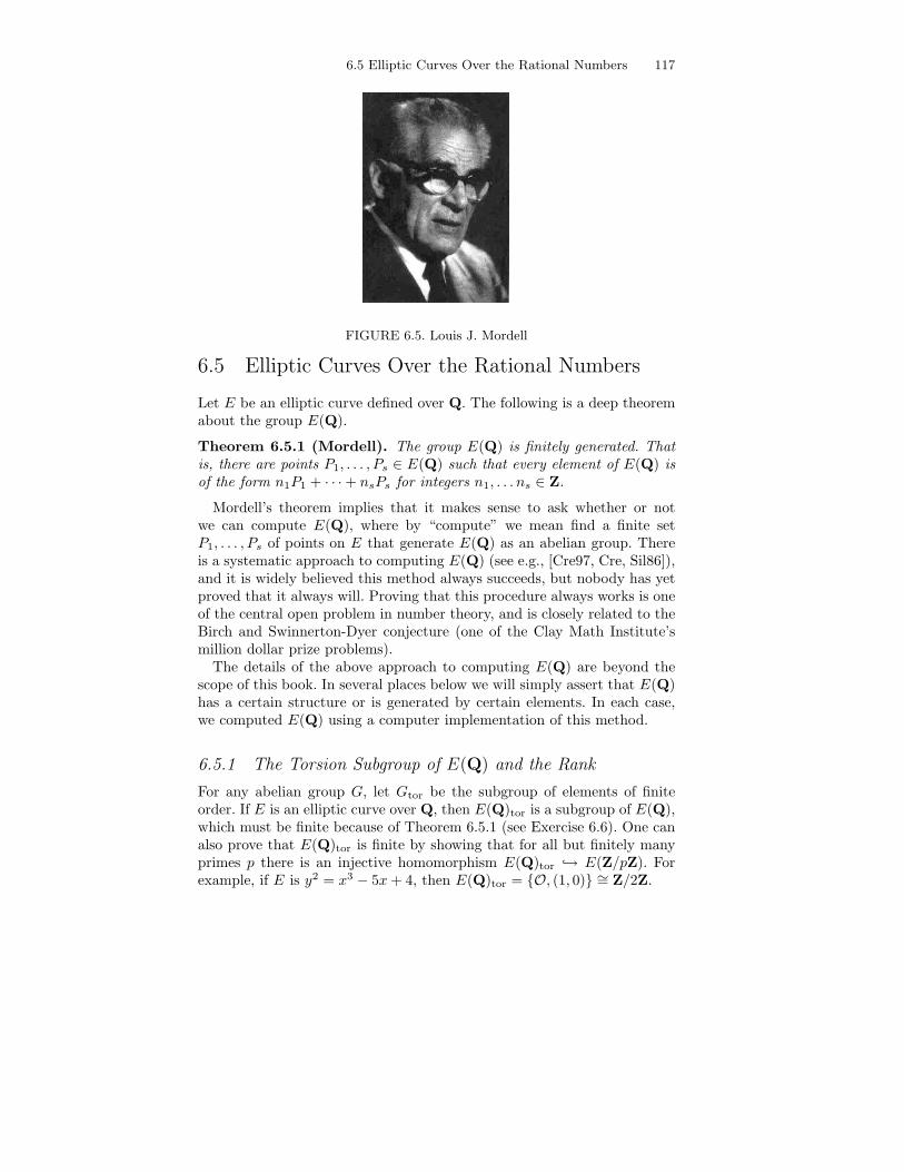
6.5 Elliptic Curves Over the Rational Numbers 117
FIGURE 6.5. Louis J. Mordell
6.5 Elliptic Curves Over the Rational Numbers
Let E be an elliptic curve defined over Q. The following is a deep theoremabout the group E(Q).
Theorem 6.5.1 (Mordell). The group E(Q) is finitely generated. Thatis, there are points P1, . . . , Ps ∈ E(Q) such that every element of E(Q) isof the form n1P1 + · · · + nsPs for integers n1, . . . ns ∈ Z.
Mordell’s theorem implies that it makes sense to ask whether or notwe can compute E(Q), where by “compute” we mean find a finite setP1, . . . , Ps of points on E that generate E(Q) as an abelian group. Thereis a systematic approach to computing E(Q) (see e.g., [Cre97, Cre, Sil86]),and it is widely believed this method always succeeds, but nobody has yetproved that it always will. Proving that this procedure always works is oneof the central open problem in number theory, and is closely related to theBirch and Swinnerton-Dyer conjecture (one of the Clay Math Institute’smillion dollar prize problems).
The details of the above approach to computing E(Q) are beyond thescope of this book. In several places below we will simply assert that E(Q)has a certain structure or is generated by certain elements. In each case,we computed E(Q) using a computer implementation of this method.
6.5.1 The Torsion Subgroup of E(Q) and the Rank
For any abelian group G, let Gtor be the subgroup of elements of finiteorder. If E is an elliptic curve over Q, then E(Q)tor is a subgroup of E(Q),which must be finite because of Theorem 6.5.1 (see Exercise 6.6). One canalso prove that E(Q)tor is finite by showing that for all but finitely manyprimes p there is an injective homomorphism E(Q)tor → E(Z/pZ). Forexample, if E is y2 = x3 − 5x + 4, then E(Q)tor = {O, (1, 0)} ∼= Z/2Z.
118 6. Elliptic Curves
The possibilities for E(Q)tor are known.
Theorem 6.5.2 (Mazur, 1976). Let E be an elliptic curve over Q. ThenE(Q)tor is isomorphic to one of the following 15 groups:
Z/nZ for n ≤ 10 or n = 12,
Z/2 × Z/2n for n ≤ 4.
The quotient E(Q)/E(Q)tor is a finitely generated free abelian group,so it is isomorphism to Zr for some integer r, called the rank of E(Q).
Conjecture 6.5.3. There are elliptic curves over Q of arbitrarily largerank.
The “world record” is the following curve, whose rank is at least 24:
y2+xy + y = x3 − 120039822036992245303534619191166796374x
+ 504224992484910670010801799168082726759443756222911415116
It was discovered in January 2000 by Roland Martin and William McMillenof the National Security Agency. For several months they were not allowedto release the actual curve to the public.
6.5.2 The Congruent Number Problem
Definition 6.5.4 (Congruent Number). We call a nonzero rationalnumber n a congruent number if ±n is the area of a right triangle withrational side lengths. Equivalently, n is a congruent number if the systemof two equations
a2 + b2 = c2
1
2ab = n
has a solution with a, b, c ∈ Q.
For example, 6 is the area of the right triangle with side lengths 3, 4,and 5, so 6 is a congruent number. Less obvious is that 5 is also a congruentnumber; it is the area of the right triangle with side lengths 3/2, 20/3, and41/6. It is nontrivial to prove that 1, 2, 3, and 4 are not congruent numbers.Here is a list of the integer congruent numbers up to 50:
5, 6, 7, 13, 14, 15, 20, 21, 22, 23, 24, 28, 29, 30, 31, 34, 37, 38, 39, 41, 45, 46, 47.
Every congruence class modulo 8 except 3 is represented in this list,which incorrectly suggests that if n ≡ 3 (mod 8) then n is not a congruentnumber. Though no n ≤ 218 with n ≡ 3 (mod 8) is a congruent number,n = 219 is a congruent number congruent and 219 ≡ 3 (mod 8).
6.5 Elliptic Curves Over the Rational Numbers 119
Deciding whether an integer n is a congruent number can be subtle sincethe simplest triangle with area n can be very complicated. For example,as Zagier pointed out, the number 157 is a congruent number, and the“simplest” rational right triangle with area 157 has side lengths
a =6803298487826435051217540
411340519227716149383203and b =
411340519227716149383203
21666555693714761309610.
This solution would be difficult to find by a brute force search.We call congruent numbers “congruent” because of the following proposi-
tion, which asserts that any congruent number is the common “congruence”between three perfect squares.
Proposition 6.5.5. Suppose n is the area of a right triangle with rationalside lengths a, b, c, with a ≤ b < c. Let A = (c/2)2. Then
A − n, A, and A + n
are all perfect squares of rational numbers.
Proof. We have
a2 + b2 = c2
1
2ab = n
Add or subtract 4 times the second equation to the first to get
a2 ± 2ab + b2 = c2 ± 4n
(a ± b)2 = c2 ± 4n(
a ± b
2
)2
=( c
2
)2
± n
= A ± n
The following open problem has motivated much work on congruent num-bers.
Open Problem 6.5.6. Give an algorithm which, given n, outputs whetheror not n is a congruent number.
The following proposition establishes a link between elliptic curves andthe congruent number problem.
Proposition 6.5.7 (Congruent numbers and elliptic curves). Let nbe a rational number. There is a bijection between
A =
{
(a, b, c) ∈ Q3 :ab
2= n, a2 + b2 = c2
}
120 6. Elliptic Curves
and
B ={
(x, y) ∈ Q2 : y2 = x3 − n2x, with y 6= 0}
given explicitly by the maps
f(a, b, c) =
(
− nb
a + c, 2n2a + c
)
and
g(x, y) =
(
n2 − x2
y, −2xn
y,
n2 + x2
y
)
.
The proof of this proposition is not deep, but involves substantial algebraand we will not prove it in this book.
For n 6= 0, let En be the elliptic curve y2 = x3 − n2x.
Proposition 6.5.8 (Congruent number criterion). The rational num-ber n is a congruent number if and only if there is a point P = (x, y) ∈En(Q) with y 6= 0.
Proof. The number n is a congruent number if and only if the set A fromProposition 6.5.7 is nonempty. By the proposition A is nonempty if andonly if B is nonempty.
Example 6.5.9. Let n = 5. Then En is y2 = x3 − 25x, and we find by abrute force search the point (−4,−6) ∈ En(Q). Then
g(−4,−6) =
(
25 − 16
−6,−−40
−6,25 + 16
−6
)
=
(
−3
2,−20
3,−41
6
)
.
Multiplying through by −1 yields the side lengths of a rational right trianglewith area 5.
We can apply the map g to any point in En(Q) with y 6= 0. Using thegroup law we find that 2(−4,−6) = (1681/144, 62279/1728), and
g(2(−4,−6)) =
(
−1519
492,−4920
1519,3344161
747348
)
.
Example 6.5.10. Let n = 1, so E1 is defined by y2 = x3 − x. Since 1 is nota congruent number, the elliptic curve E1 has no point with y 6= 0. SeeExercise 6.10.
Example 6.5.9 foreshadows the following theorem.
Theorem 6.5.11 (Infinitely Many Triangles). If n is a congruentnumber, then there are infinitely many distinct right triangles with rationalside lengths and area n.
6.6 Exercises 121
We will not prove this theorem, except to note that one proves it byshowing that En(Q)tor = {O, (0, 0), (n, 0), (−n, 0)}, so the elements of theset B in Proposition 6.5.7 all have infinite order, hence B is infinite so Ais infinite.
There is a theorem of Tunnell that combined with the conjecture ofBirch and Swinnerton-Dyer (alluded to above), which if true, would implythe existence of an elementary way to decide whether or not an integer nis a congruent number. We state this elementary way in the form of aconjecture.
Conjecture 6.5.12. Let a, b, c denote integers. If n is an even square-freeinteger then n is a congruent number if and only if
#{
(a, b, c) ∈ Z3 : 4a2 + b2 + 8c2 =n
2: c is even
}
= #{
(a, b, c) : 4a2 + b2 + 8c2 =n
2: c is odd
}
.
If n is odd and square free then n is a congruent number if and only if
#{
(a, b, c) : 2a2 + b2 + 8c2 = n : c is even}
= #{
(a, b, c) : 2a2 + b2 + 8c2 = n : c is odd}
.
The book [Kob84] is about congruent numbers and Conjecture 6.5.12.The Birch and Swinnerton-Dyer conjecture is a Clay Math Institute milliondollar millennium prize problem (see [Cla, Wil00]).
6.6 Exercises
6.1 Write down an equation y2 = x3 + ax + b over a field K such that−16(4a3+27b2) = 0. Precisely what goes wrong when trying to endowthe set E(K) = {(x, y) ∈ K × K : y2 = x3 + ax + b} ∪ {O} with agroup structure?
6.2 One rational solution to the equation y2 = x3 − 2 is (3, 5). Find arational solution with x 6= 3 by drawing the tangent line to (3, 5) andcomputing the second point of intersection.
6.3 Let E be the elliptic curve over the finite field K = Z/5Z defined bythe equation
y2 = x3 + x + 1.
(a) List all 9 elements of E(K).
(b) What is the structure of E(K), as a product of cyclic groups?
122 6. Elliptic Curves
6.4 Let E be the elliptic curve defined by the equation y2 = x3 + 1. Foreach prime p ≥ 5, let Np be the cardinality of the group E(Z/pZ)of points on this curve having coordinates in Z/pZ. For example, wehave that N5 = 6, N7 = 12, N11 = 12, N13 = 12, N17 = 18, N19 =12, , N23 = 24, and N29 = 30 (you do not have to prove this).
(a) For the set of primes satisfying p ≡ 2 (mod 3), can you see apattern for the values of Np? Make a general conjecture for thevalue of Np when p ≡ 2 (mod 3).
(b) (*) Prove your conjecture.
6.5 Let E be an elliptic curve over the real numbers R. Prove that E(R)is not a finitely generated abelian group.
6.6 (*) Suppose G is a finitely generated abelian group. Prove that thesubgroup Gtor of elements of finite order in G is finite.
6.7 Suppose y2 = x3 +ax+b with a, b ∈ Q defines an elliptic curve. Showthat there is another equation Y 2 = X3 + AX + B with A,B ∈ Zwhose solutions are in bijection with the solutions to y2 = x3+ax+b.
6.8 Suppose a, b, c are relatively prime integers with a2 + b2 = c2. Thenthere exist integers x and y with x > y such that c = x2 + y2 andeither a = x2 − y2, b = 2xy or a = 2xy, b = x2 − y2.
6.9 (*) Fermat’s Last Theorem for exponent 4 asserts that any solutionto the equation x4 + y4 = z4 with x, y, z ∈ Z satisfies xyz = 0. Proveof Fermat’s Last Theorem for exponent 4, as follows.
(a) Show that if the equation x2 + y4 = z4 has no integer solutionswith xyz 6= 0, then Fermat’s Last Theorem for exponent 4 istrue.
(b) Prove that x2 +y4 = z4 has no integer solutions with xyz 6= 0 asfollows. Suppose n2 +k4 = m4 is a solution with m > 0 minimalamongst all solutions. Show that there exists a solution with msmaller using Exercise 6.8 (consider two cases).
6.10 (*) Prove that 1 is not a congruent number by showing that theelliptic curve y2 = x3 − x has no rational solutions except (0, 1) and(0, 0), as follows:
(a) Write y = pq and x = r
s , where p, q, r, s are all positive integers
and gcd(p, q) = gcd(r, s) = 1. Prove that s | q, so q = sk forsome k ∈ Z.
(b) Prove that s = k2, and substitute to see that p2 = r3 − rk4.
6.6 Exercises 123
(c) Prove that r is a perfect square by supposing there is a prime ℓsuch that ordℓ(r) is odd and analyzing ordℓ of both sides ofp2 = r3 − rk4.
(d) Write r = m2, and substitute to see that p2 = m6−m2k4. Provethat m | p.
(e) Divide through by m2 and deduce a contradiction to Exer-cise 6.9.

124 6. Elliptic Curves
This is page 125Printer: Opaque this
7Computational Number Theory
In this chapter, we discuss how to use the computer language Python todo computations with many of the mathematical objects discussed in thisbook. One reason we separate this chapter from the other chapters is thatthe best order for presenting theory is in many cases not the best order forpresenting algorithms that rely on that theory. For example, in Section 2.1.1we gave theoretical criterion for whether or not a linear equation ax ≡ b(mod n) has a solution, and it wasn’t until Section 2.3 that we describedan algorithm for solving them. Moreover, extensive asides on issues relatedto implementing algorithms would obstruct the flow of the earlier chapters.
We use Python [Ros] because it is free and includes arbitrary precisioninteger arithmetic, but does not include substantial number theoretic func-tionality. If we were to use one of the major packages such as Mathematica,Maple, MATLAB, or MAGMA, then this chapter would be a manual de-scribing how to use various builtin functions, instead of a chapter abouthow those functions actually work. Also, Python code is concise and easyto read. A drawback to using Python is that some of the algorithms we im-plemented for this book run more slowly than they would if implementedin certain other languages. We believe the clarity of having complete im-plementations of the relevant algorithms for this book easily available in areadable form is worth the tradeoff.
If you do not wish to use Python, you can still learn from this chapter.View the Python listings as pseudocode, and try to understand the detailsof how the algorithms work. In contrast, if you would like to understandPython well, great places to start are http://docs.python.org/tut and
126 7. Computational Number Theory
http://diveintopython.org. Also, in this chapter we will describe newlanguage feature as we first encounter them.
Python is freely available from http://www.python.org. The examplesin this chapter assume you are using Python version at least 2.3. You candownload a file that contains all of the code printed on the following pagesfrom
http://modular.fas.harvard.edu/ent/.
Put the file ent.py in a directory, start up Python, and load the functionsfrom ent.py by typing the following:
>>> from ent import *
You might also install IPython (http://ipython.scipy.org), whichprovides a friendly interface to Python with better support for mathematicsand documentation.
The examples in this chapter have been automatically tested using thedefault Python 2.3 shell. Some examples contain numbers that are obtainedusing randomized algorithms, so output may be different for you. Linescontaining such output are indicated by a comment #rand.
Some of the functions defined in this chapter use the Python functionslog and sqrt from the Python math library, and the randrange functionfrom the random library. The code below assume these three functions havebeen imported as follows:
from random import randrange
from math import log, sqrt
In Python the notation == means “equals”, != means “not equals”, >=means ≥ and <= means ≤. Another important convention in Python is thatif n and m are integers, then the expression n/m evaluates to the biggestinteger ≤ n/m, as the following examples illustrate:
>>> 7/5
1
>>> -2/3
-1
To obtain a floating point approximation to a rational number use adecimal point or coerce at least one of the integers to a float
>>> 1.0/3
0.33333333333333331
>>> float(2)/3
0.66666666666666663
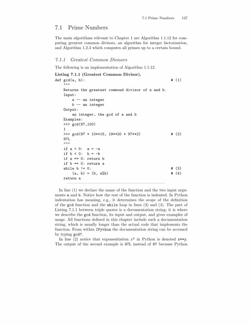
7.1 Prime Numbers 127
7.1 Prime Numbers
The main algorithms relevant to Chapter 1 are Algorithm 1.1.12 for com-puting greatest common divisors, an algorithm for integer factorization,and Algorithm 1.2.3 which computes all primes up to a certain bound.
7.1.1 Greatest Common Divisors
The following is an implementation of Algorithm 1.1.12.
Listing 7.1.1 (Greatest Common Divisor).
def gcd(a, b): # (1)
"""
Returns the greatest commond divisor of a and b.
Input:
a -- an integer
b -- an integer
Output:
an integer, the gcd of a and b
Examples:
>>> gcd(97,100)
1
>>> gcd(97 * 10**15, 19**20 * 97**2) # (2)
97L
"""
if a < 0: a = -a
if b < 0: b = -b
if a == 0: return b
if b == 0: return a
while b != 0: # (3)
(a, b) = (b, a%b) # (4)
return a
————————————————————————
In line (1) we declare the name of the function and the two input argu-ments a and b. Notice how the rest of the function is indented. In Pythonindentation has meaning, e.g., it determines the scope of the definitionof the gcd function and the while loop in lines (3) and (4). The part ofListing 7.1.1 between triple quotes is a documentation string; it is wherewe describe the gcd function, its input and output, and gives examples ofusage. All functions defined in this chapter include such a documentationstring, which is usually longer than the actual code that implements thefunction. From within IPython the documentation string can be accessedby typing gcd?.
In line (2) notice that exponentiation xy in Python is denoted x**y.The output of the second example is 97L instead of 97 because Python
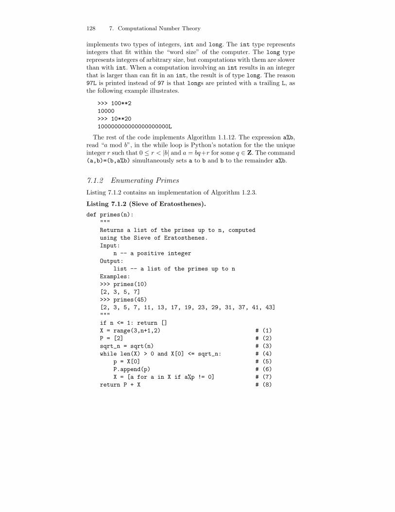
128 7. Computational Number Theory
implements two types of integers, int and long. The int type representsintegers that fit within the “word size” of the computer. The long typerepresents integers of arbitrary size, but computations with them are slowerthan with int. When a computation involving an int results in an integerthat is larger than can fit in an int, the result is of type long. The reason97L is printed instead of 97 is that longs are printed with a trailing L, asthe following example illustrates.
>>> 100**2
10000
>>> 10**20
100000000000000000000L
The rest of the code implements Algorithm 1.1.12. The expression a%b,read “a mod b”, in the while loop is Python’s notation for the the uniqueinteger r such that 0 ≤ r < |b| and a = bq+r for some q ∈ Z. The command(a,b)=(b,a%b) simultaneously sets a to b and b to the remainder a%b.
7.1.2 Enumerating Primes
Listing 7.1.2 contains an implementation of Algorithm 1.2.3.
Listing 7.1.2 (Sieve of Eratosthenes).
def primes(n):
"""
Returns a list of the primes up to n, computed
using the Sieve of Eratosthenes.
Input:
n -- a positive integer
Output:
list -- a list of the primes up to n
Examples:
>>> primes(10)
[2, 3, 5, 7]
>>> primes(45)
[2, 3, 5, 7, 11, 13, 17, 19, 23, 29, 31, 37, 41, 43]
"""
if n <= 1: return []
X = range(3,n+1,2) # (1)
P = [2] # (2)
sqrt_n = sqrt(n) # (3)
while len(X) > 0 and X[0] <= sqrt_n: # (4)
p = X[0] # (5)
P.append(p) # (6)
X = [a for a in X if a%p != 0] # (7)
return P + X # (8)
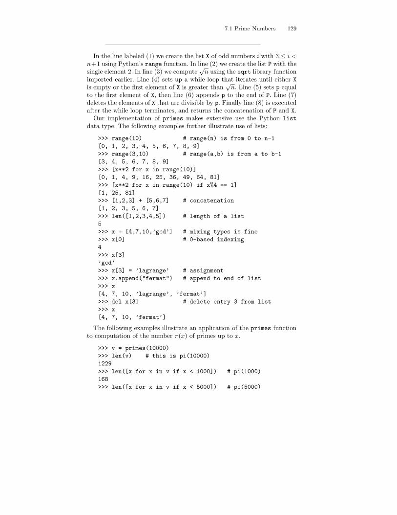
7.1 Prime Numbers 129
————————————————————————
In the line labeled (1) we create the list X of odd numbers i with 3 ≤ i <n+1 using Python’s range function. In line (2) we create the list P with thesingle element 2. In line (3) we compute
√n using the sqrt library function
imported earlier. Line (4) sets up a while loop that iterates until either X
is empty or the first element of X is greater than√
n. Line (5) sets p equalto the first element of X, then line (6) appends p to the end of P. Line (7)deletes the elements of X that are divisible by p. Finally line (8) is executedafter the while loop terminates, and returns the concatenation of P and X.
Our implementation of primes makes extensive use the Python list
data type. The following examples further illustrate use of lists:
>>> range(10) # range(n) is from 0 to n-1
[0, 1, 2, 3, 4, 5, 6, 7, 8, 9]
>>> range(3,10) # range(a,b) is from a to b-1
[3, 4, 5, 6, 7, 8, 9]
>>> [x**2 for x in range(10)]
[0, 1, 4, 9, 16, 25, 36, 49, 64, 81]
>>> [x**2 for x in range(10) if x%4 == 1]
[1, 25, 81]
>>> [1,2,3] + [5,6,7] # concatenation
[1, 2, 3, 5, 6, 7]
>>> len([1,2,3,4,5]) # length of a list
5
>>> x = [4,7,10,’gcd’] # mixing types is fine
>>> x[0] # 0-based indexing
4
>>> x[3]
’gcd’
>>> x[3] = ’lagrange’ # assignment
>>> x.append("fermat") # append to end of list
>>> x
[4, 7, 10, ’lagrange’, ’fermat’]
>>> del x[3] # delete entry 3 from list
>>> x
[4, 7, 10, ’fermat’]
The following examples illustrate an application of the primes functionto computation of the number π(x) of primes up to x.
>>> v = primes(10000)
>>> len(v) # this is pi(10000)
1229
>>> len([x for x in v if x < 1000]) # pi(1000)
168
>>> len([x for x in v if x < 5000]) # pi(5000)
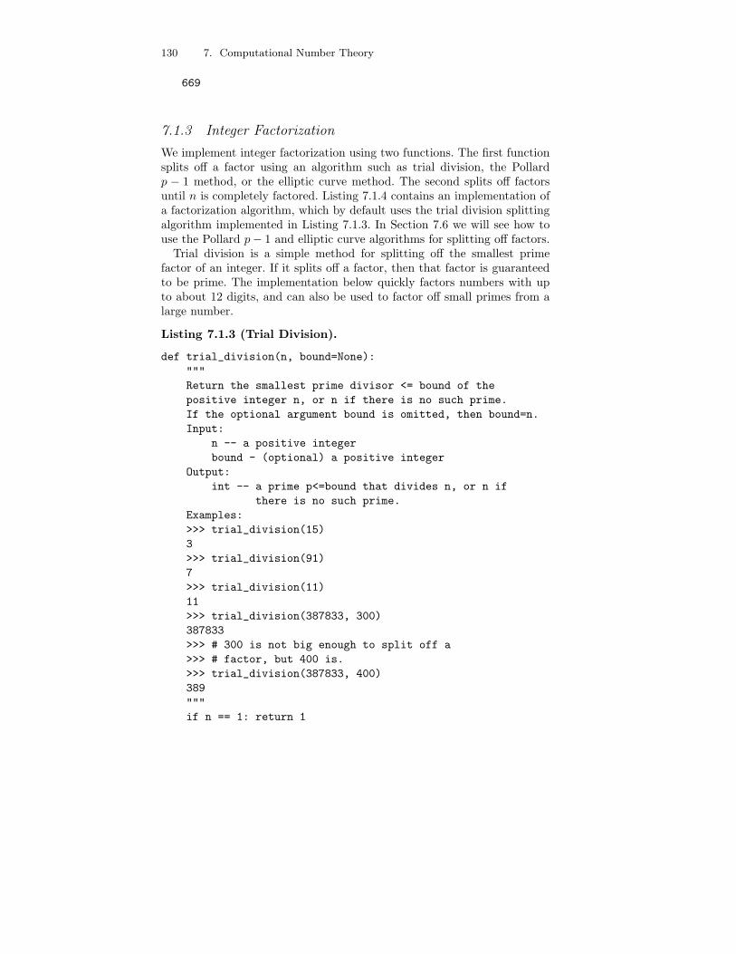
130 7. Computational Number Theory
669
7.1.3 Integer Factorization
We implement integer factorization using two functions. The first functionsplits off a factor using an algorithm such as trial division, the Pollardp − 1 method, or the elliptic curve method. The second splits off factorsuntil n is completely factored. Listing 7.1.4 contains an implementation ofa factorization algorithm, which by default uses the trial division splittingalgorithm implemented in Listing 7.1.3. In Section 7.6 we will see how touse the Pollard p − 1 and elliptic curve algorithms for splitting off factors.
Trial division is a simple method for splitting off the smallest primefactor of an integer. If it splits off a factor, then that factor is guaranteedto be prime. The implementation below quickly factors numbers with upto about 12 digits, and can also be used to factor off small primes from alarge number.
Listing 7.1.3 (Trial Division).
def trial_division(n, bound=None):
"""
Return the smallest prime divisor <= bound of the
positive integer n, or n if there is no such prime.
If the optional argument bound is omitted, then bound=n.
Input:
n -- a positive integer
bound - (optional) a positive integer
Output:
int -- a prime p<=bound that divides n, or n if
there is no such prime.
Examples:
>>> trial_division(15)
3
>>> trial_division(91)
7
>>> trial_division(11)
11
>>> trial_division(387833, 300)
387833
>>> # 300 is not big enough to split off a
>>> # factor, but 400 is.
>>> trial_division(387833, 400)
389
"""
if n == 1: return 1
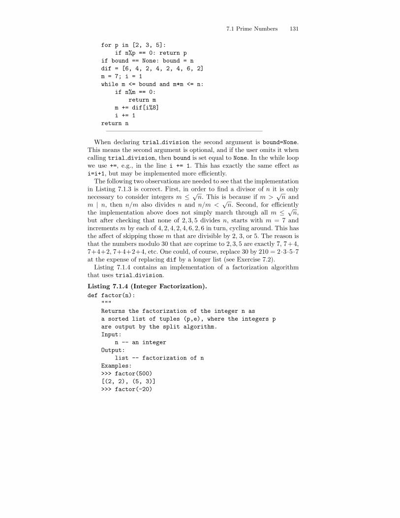
7.1 Prime Numbers 131
for p in [2, 3, 5]:
if n%p == 0: return p
if bound == None: bound = n
dif = [6, 4, 2, 4, 2, 4, 6, 2]
m = 7; i = 1
while m <= bound and m*m <= n:
if n%m == 0:
return m
m += dif[i%8]
i += 1
return n
————————————————————————
When declaring trial division the second argument is bound=None.This means the second argument is optional, and if the user omits it whencalling trial division, then bound is set equal to None. In the while loopwe use +=, e.g., in the line i += 1. This has exactly the same effect asi=i+1, but may be implemented more efficiently.
The following two observations are needed to see that the implementationin Listing 7.1.3 is correct. First, in order to find a divisor of n it is onlynecessary to consider integers m ≤ √
n. This is because if m >√
n andm | n, then n/m also divides n and n/m <
√n. Second, for efficiently
the implementation above does not simply march through all m ≤ √n,
but after checking that none of 2, 3, 5 divides n, starts with m = 7 andincrements m by each of 4, 2, 4, 2, 4, 6, 2, 6 in turn, cycling around. This hasthe affect of skipping those m that are divisible by 2, 3, or 5. The reason isthat the numbers modulo 30 that are coprime to 2, 3, 5 are exactly 7, 7+4,7+4+2, 7+4+2+4, etc. One could, of course, replace 30 by 210 = 2·3·5·7at the expense of replacing dif by a longer list (see Exercise 7.2).
Listing 7.1.4 contains an implementation of a factorization algorithmthat uses trial division.
Listing 7.1.4 (Integer Factorization).
def factor(n):
"""
Returns the factorization of the integer n as
a sorted list of tuples (p,e), where the integers p
are output by the split algorithm.
Input:
n -- an integer
Output:
list -- factorization of n
Examples:
>>> factor(500)
[(2, 2), (5, 3)]
>>> factor(-20)
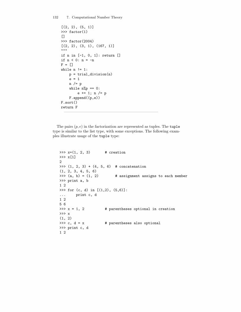
132 7. Computational Number Theory
[(2, 2), (5, 1)]
>>> factor(1)
[]
>>> factor(2004)
[(2, 2), (3, 1), (167, 1)]
"""
if n in [-1, 0, 1]: return []
if n < 0: n = -n
F = []
while n != 1:
p = trial_division(n)
e = 1
n /= p
while n%p == 0:
e += 1; n /= p
F.append((p,e))
F.sort()
return F
————————————————————————
The pairs (p, e) in the factorization are represented as tuples. The tupletype is similar to the list type, with some exceptions. The following exam-ples illustrate usage of the tuple type:
>>> x=(1, 2, 3) # creation
>>> x[1]
2
>>> (1, 2, 3) + (4, 5, 6) # concatenation
(1, 2, 3, 4, 5, 6)
>>> (a, b) = (1, 2) # assignment assigns to each member
>>> print a, b
1 2
>>> for (c, d) in [(1,2), (5,6)]:
... print c, d
1 2
5 6
>>> x = 1, 2 # parentheses optional in creation
>>> x
(1, 2)
>>> c, d = x # parentheses also optional
>>> print c, d
1 2
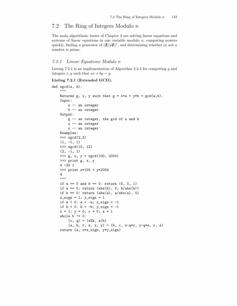
7.2 The Ring of Integers Modulo n 133
7.2 The Ring of Integers Modulo n
The main algorithmic issues of Chapter 2 are solving linear equations andsystems of linear equations in one variable modulo n, computing powersquickly, finding a generator of (Z/pZ)∗, and determining whether or not anumber is prime.
7.2.1 Linear Equations Modulo n
Listing 7.2.1 is an implementation of Algorithm 2.3.4 for computing g andintegers x, y such that ax + by = g.
Listing 7.2.1 (Extended GCD).
def xgcd(a, b):
"""
Returns g, x, y such that g = x*a + y*b = gcd(a,b).
Input:
a -- an integer
b -- an integer
Output:
g -- an integer, the gcd of a and b
x -- an integer
y -- an integer
Examples:
>>> xgcd(2,3)
(1, -1, 1)
>>> xgcd(10, 12)
(2, -1, 1)
>>> g, x, y = xgcd(100, 2004)
>>> print g, x, y
4 -20 1
>>> print x*100 + y*2004
4
"""
if a == 0 and b == 0: return (0, 0, 1)
if a == 0: return (abs(b), 0, b/abs(b))
if b == 0: return (abs(a), a/abs(a), 0)
x_sign = 1; y_sign = 1
if a < 0: a = -a; x_sign = -1
if b < 0: b = -b; y_sign = -1
x = 1; y = 0; r = 0; s = 1
while b != 0:
(c, q) = (a%b, a/b)
(a, b, r, s, x, y) = (b, c, x-q*r, y-q*s, r, s)
return (a, x*x_sign, y*y_sign)
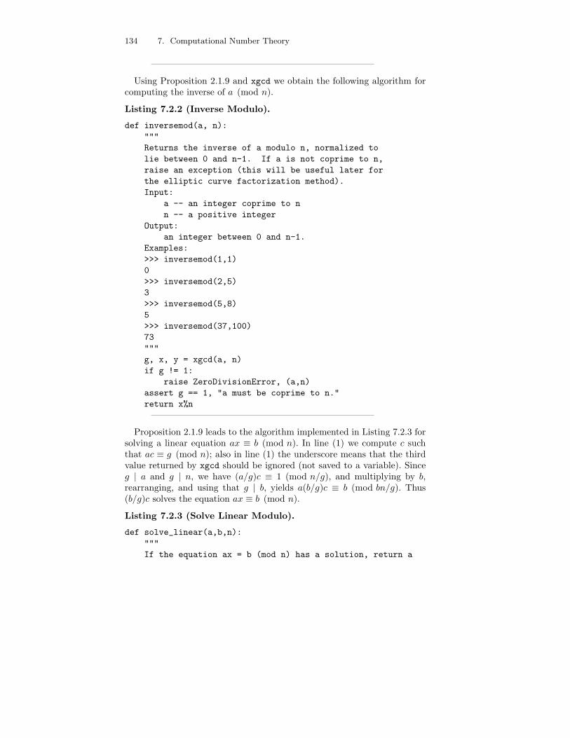
134 7. Computational Number Theory
————————————————————————
Using Proposition 2.1.9 and xgcd we obtain the following algorithm forcomputing the inverse of a (mod n).
Listing 7.2.2 (Inverse Modulo).
def inversemod(a, n):
"""
Returns the inverse of a modulo n, normalized to
lie between 0 and n-1. If a is not coprime to n,
raise an exception (this will be useful later for
the elliptic curve factorization method).
Input:
a -- an integer coprime to n
n -- a positive integer
Output:
an integer between 0 and n-1.
Examples:
>>> inversemod(1,1)
0
>>> inversemod(2,5)
3
>>> inversemod(5,8)
5
>>> inversemod(37,100)
73
"""
g, x, y = xgcd(a, n)
if g != 1:
raise ZeroDivisionError, (a,n)
assert g == 1, "a must be coprime to n."
return x%n
————————————————————————
Proposition 2.1.9 leads to the algorithm implemented in Listing 7.2.3 forsolving a linear equation ax ≡ b (mod n). In line (1) we compute c suchthat ac ≡ g (mod n); also in line (1) the underscore means that the thirdvalue returned by xgcd should be ignored (not saved to a variable). Sinceg | a and g | n, we have (a/g)c ≡ 1 (mod n/g), and multiplying by b,rearranging, and using that g | b, yields a(b/g)c ≡ b (mod bn/g). Thus(b/g)c solves the equation ax ≡ b (mod n).
Listing 7.2.3 (Solve Linear Modulo).
def solve_linear(a,b,n):
"""
If the equation ax = b (mod n) has a solution, return a
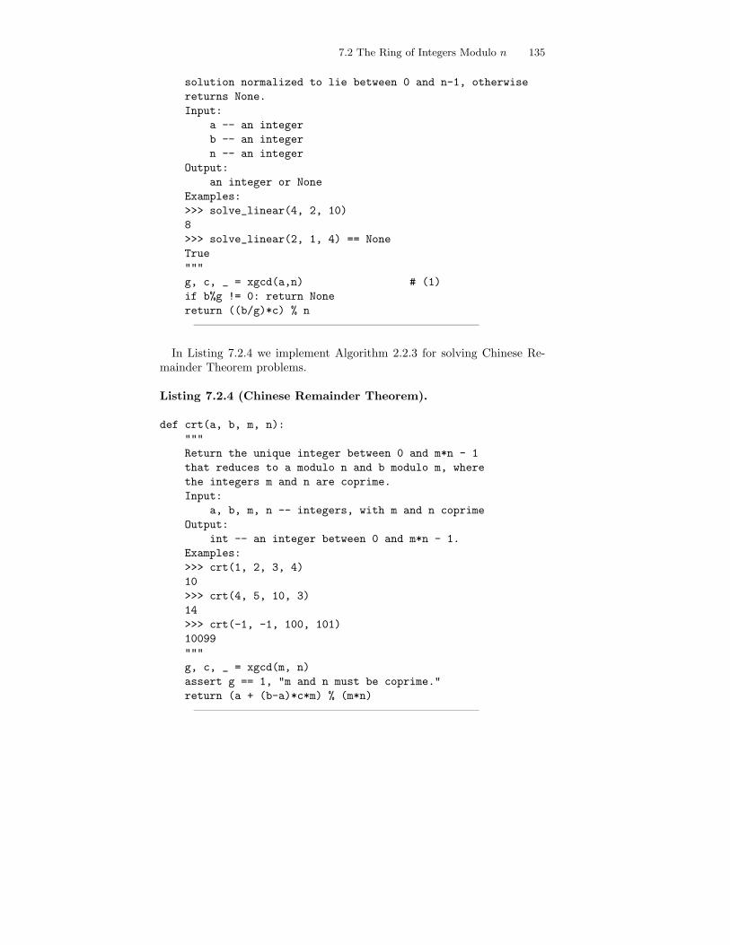
7.2 The Ring of Integers Modulo n 135
solution normalized to lie between 0 and n-1, otherwise
returns None.
Input:
a -- an integer
b -- an integer
n -- an integer
Output:
an integer or None
Examples:
>>> solve_linear(4, 2, 10)
8
>>> solve_linear(2, 1, 4) == None
True
"""
g, c, _ = xgcd(a,n) # (1)
if b%g != 0: return None
return ((b/g)*c) % n
————————————————————————
In Listing 7.2.4 we implement Algorithm 2.2.3 for solving Chinese Re-mainder Theorem problems.
Listing 7.2.4 (Chinese Remainder Theorem).
def crt(a, b, m, n):
"""
Return the unique integer between 0 and m*n - 1
that reduces to a modulo n and b modulo m, where
the integers m and n are coprime.
Input:
a, b, m, n -- integers, with m and n coprime
Output:
int -- an integer between 0 and m*n - 1.
Examples:
>>> crt(1, 2, 3, 4)
10
>>> crt(4, 5, 10, 3)
14
>>> crt(-1, -1, 100, 101)
10099
"""
g, c, _ = xgcd(m, n)
assert g == 1, "m and n must be coprime."
return (a + (b-a)*c*m) % (m*n)
————————————————————————
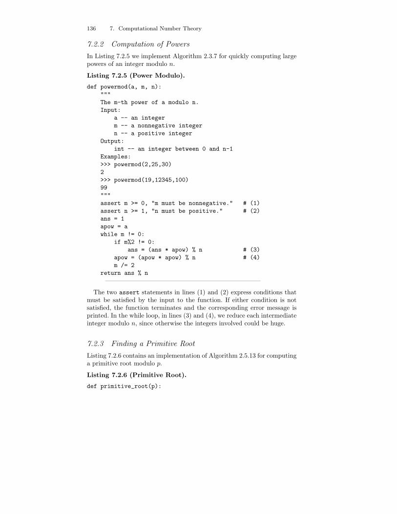
136 7. Computational Number Theory
7.2.2 Computation of Powers
In Listing 7.2.5 we implement Algorithm 2.3.7 for quickly computing largepowers of an integer modulo n.
Listing 7.2.5 (Power Modulo).
def powermod(a, m, n):
"""
The m-th power of a modulo n.
Input:
a -- an integer
m -- a nonnegative integer
n -- a positive integer
Output:
int -- an integer between 0 and n-1
Examples:
>>> powermod(2,25,30)
2
>>> powermod(19,12345,100)
99
"""
assert m >= 0, "m must be nonnegative." # (1)
assert n >= 1, "n must be positive." # (2)
ans = 1
apow = a
while m != 0:
if m%2 != 0:
ans = (ans * apow) % n # (3)
apow = (apow * apow) % n # (4)
m /= 2
return ans % n
————————————————————————
The two assert statements in lines (1) and (2) express conditions thatmust be satisfied by the input to the function. If either condition is notsatisfied, the function terminates and the corresponding error message isprinted. In the while loop, in lines (3) and (4), we reduce each intermediateinteger modulo n, since otherwise the integers involved could be huge.
7.2.3 Finding a Primitive Root
Listing 7.2.6 contains an implementation of Algorithm 2.5.13 for computinga primitive root modulo p.
Listing 7.2.6 (Primitive Root).
def primitive_root(p):
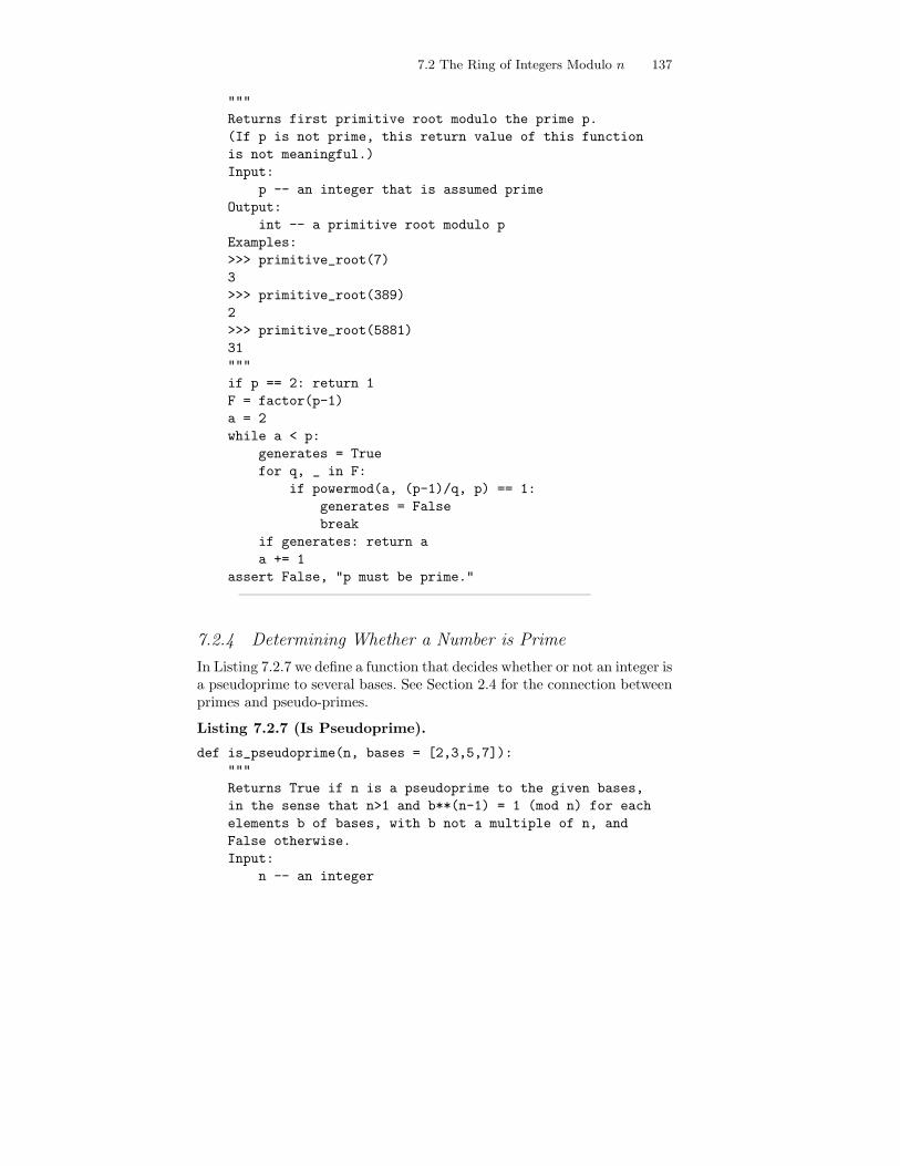
7.2 The Ring of Integers Modulo n 137
"""
Returns first primitive root modulo the prime p.
(If p is not prime, this return value of this function
is not meaningful.)
Input:
p -- an integer that is assumed prime
Output:
int -- a primitive root modulo p
Examples:
>>> primitive_root(7)
3
>>> primitive_root(389)
2
>>> primitive_root(5881)
31
"""
if p == 2: return 1
F = factor(p-1)
a = 2
while a < p:
generates = True
for q, _ in F:
if powermod(a, (p-1)/q, p) == 1:
generates = False
break
if generates: return a
a += 1
assert False, "p must be prime."
————————————————————————
7.2.4 Determining Whether a Number is Prime
In Listing 7.2.7 we define a function that decides whether or not an integer isa pseudoprime to several bases. See Section 2.4 for the connection betweenprimes and pseudo-primes.
Listing 7.2.7 (Is Pseudoprime).
def is_pseudoprime(n, bases = [2,3,5,7]):
"""
Returns True if n is a pseudoprime to the given bases,
in the sense that n>1 and b**(n-1) = 1 (mod n) for each
elements b of bases, with b not a multiple of n, and
False otherwise.
Input:
n -- an integer

138 7. Computational Number Theory
bases -- a list of integers
Output:
bool
Examples:
>>> is_pseudoprime(91)
False
>>> is_pseudoprime(97)
True
>>> is_pseudoprime(1)
False
>>> is_pseudoprime(-2)
True
>>> s = [x for x in range(10000) if is_pseudoprime(x)]
>>> t = primes(10000)
>>> s == t
True
>>> is_pseudoprime(29341) # first non-prime pseudoprime
True
>>> factor(29341)
[(13, 1), (37, 1), (61, 1)]
"""
if n < 0: n = -n
if n <= 1: return False
for b in bases:
if b%n != 0 and powermod(b, n-1, n) != 1:
return False
return True
————————————————————————
We iterate over the elements b of bases, and for each b that is not amultiple of n, we decide whether bn−1 ≡ 1 (mod n). If not, then n isdefinitely not prime so we return False; if the congruence is satisfied forall b, return True.
The following session illustrates that for the default bases 2, 3, 5, 7, thefirst non-prime pseudoprime is 29341, and for the bases 2, 3, 5, 7, 11, 13,then the first non-prime pseudoprime is 162401:
>>> P = [p for p in range(200000) if is_pseudoprime(p)]
>>> Q = primes(200000)
>>> R = [x for x in P if not (x in Q)]; print R
[29341, 46657, 75361, 115921, 162401]
>>> [n for n in R if is_pseudoprime(n,[2,3,5,7,11,13])]
[162401]
>>> factor(162401)
[(17, 1), (41, 1), (233, 1)]
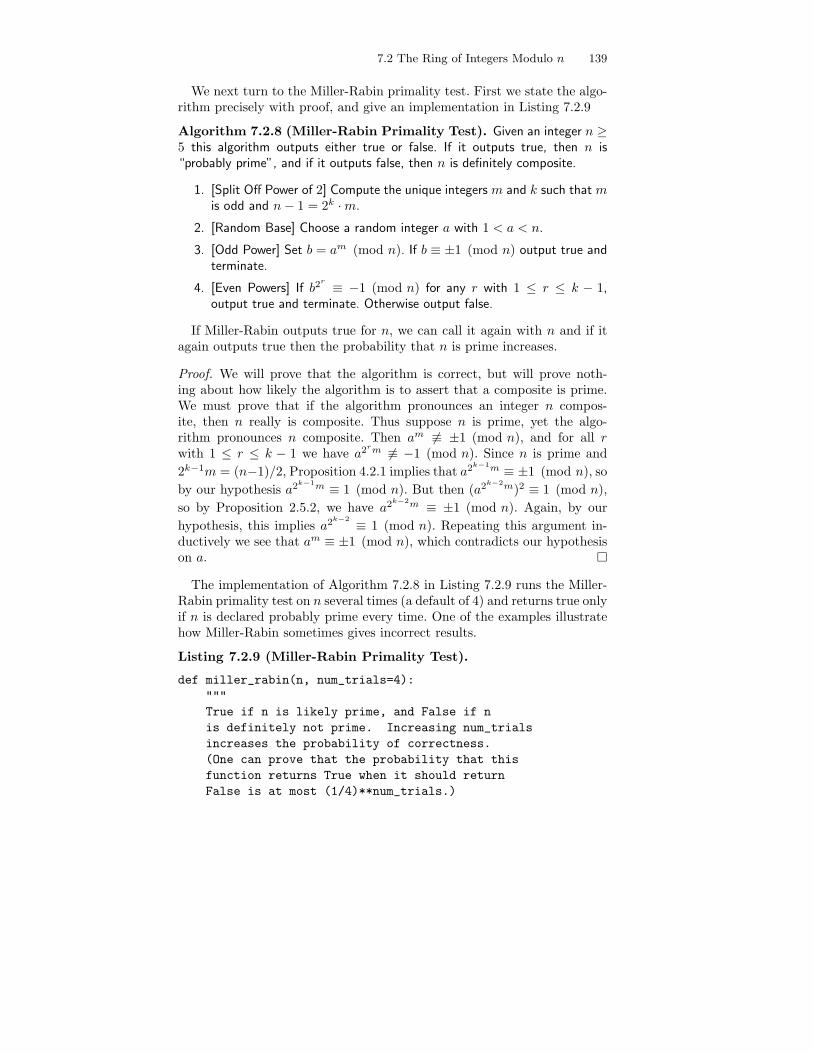
7.2 The Ring of Integers Modulo n 139
We next turn to the Miller-Rabin primality test. First we state the algo-rithm precisely with proof, and give an implementation in Listing 7.2.9
Algorithm 7.2.8 (Miller-Rabin Primality Test). Given an integer n ≥5 this algorithm outputs either true or false. If it outputs true, then n is“probably prime”, and if it outputs false, then n is definitely composite.
1. [Split Off Power of 2] Compute the unique integers m and k such that mis odd and n − 1 = 2k · m.
2. [Random Base] Choose a random integer a with 1 < a < n.
3. [Odd Power] Set b = am (mod n). If b ≡ ±1 (mod n) output true andterminate.
4. [Even Powers] If b2r ≡ −1 (mod n) for any r with 1 ≤ r ≤ k − 1,output true and terminate. Otherwise output false.
If Miller-Rabin outputs true for n, we can call it again with n and if itagain outputs true then the probability that n is prime increases.
Proof. We will prove that the algorithm is correct, but will prove noth-ing about how likely the algorithm is to assert that a composite is prime.We must prove that if the algorithm pronounces an integer n compos-ite, then n really is composite. Thus suppose n is prime, yet the algo-rithm pronounces n composite. Then am 6≡ ±1 (mod n), and for all rwith 1 ≤ r ≤ k − 1 we have a2rm 6≡ −1 (mod n). Since n is prime and
2k−1m = (n−1)/2, Proposition 4.2.1 implies that a2k−1m ≡ ±1 (mod n), so
by our hypothesis a2k−1m ≡ 1 (mod n). But then (a2k−2m)2 ≡ 1 (mod n),
so by Proposition 2.5.2, we have a2k−2m ≡ ±1 (mod n). Again, by our
hypothesis, this implies a2k−2 ≡ 1 (mod n). Repeating this argument in-ductively we see that am ≡ ±1 (mod n), which contradicts our hypothesison a.
The implementation of Algorithm 7.2.8 in Listing 7.2.9 runs the Miller-Rabin primality test on n several times (a default of 4) and returns true onlyif n is declared probably prime every time. One of the examples illustratehow Miller-Rabin sometimes gives incorrect results.
Listing 7.2.9 (Miller-Rabin Primality Test).
def miller_rabin(n, num_trials=4):
"""
True if n is likely prime, and False if n
is definitely not prime. Increasing num_trials
increases the probability of correctness.
(One can prove that the probability that this
function returns True when it should return
False is at most (1/4)**num_trials.)
140 7. Computational Number Theory
Input:
n -- an integer
num_trials -- the number of trials with the
primality test.
Output:
bool -- whether or not n is probably prime.
Examples:
>>> miller_rabin(91)
False #rand
>>> miller_rabin(97)
True #rand
>>> s = [x for x in range(1000) if miller_rabin(x, 1)]
>>> t = primes(1000)
>>> print len(s), len(t) # so 1 in 25 wrong
175 168 #rand
>>> s = [x for x in range(1000) if miller_rabin(x)]
>>> s == t
True #rand
"""
if n < 0: n = -n
if n in [2,3]: return True
if n <= 4: return False
m = n - 1
k = 0
while m%2 == 0:
k += 1; m /= 2
# Now n - 1 = (2**k) * m with m odd
for i in range(num_trials):
a = randrange(2,n-1) # (1)
apow = powermod(a, m, n)
if not (apow in [1, n-1]):
some_minus_one = False
for r in range(k-1): # (2)
apow = (apow**2)%n
if apow == n-1:
some_minus_one = True
break # (3)
if (apow in [1, n-1]) or some_minus_one:
prob_prime = True
else:
return False
return True
————————————————————————
7.3 Public-Key Cryptography 141
In line (1) we use randrange; the command randrange(a,b) returns arandom integer in the interval [a, b−1]. Line (3) uses the break statement,which exists the immediately enclosing for or while loop; in this case thefor loop starting at line (2).
7.3 Public-Key Cryptography
The main algorithms in Chapter 3 deal with implementing the Diffie-Hellman and RSA cryptosystems, and with some attacks on RSA in specialcases. In this section we give a function for encoding an arbitrary string as asequence of numbers of some bounded size, and vice-versa, then implementeach of Diffie-Hellman and RSA.
7.3.1 The Diffie-Hellman Key Exchange
In order for two parties to agree on a secret key using Diffie-Hellman, weneed a function to generate a large random prime.
Listing 7.3.1 (Random Prime).
def random_prime(num_digits, is_prime = miller_rabin):
"""
Returns a random prime with num_digits digits.
Input:
num_digits -- a positive integer
is_prime -- (optional argment)
a function of one argument n that
returns either True if n is (probably)
prime and False otherwise.
Output:
int -- an integer
Examples:
>>> random_prime(10)
8599796717L #rand
>>> random_prime(40)
1311696770583281776596904119734399028761L #rand
"""
n = randrange(10**(num_digits-1), 10**num_digits)
if n%2 == 0: n += 1
while not is_prime(n): n += 2
return n
————————————————————————
Suppose p is a large random prime. Then it is extremely unlikely that 2will have small order modulo p, so we will use g = 2 as the base for the
142 7. Computational Number Theory
key exchange. The function dh init below computes and returns a ran-dom integer n and 2n (mod p). Thus Nikita and Michael should each calldh init with input p, and send the resulting 2n (mod p) to each other.Then each calls dh secret with the powers of 2 they received to computethe the shared secret key. After defining dh init and dh secret below, wegive a complete nontrivial example.
Listing 7.3.2 (Initialize Diffie-Hellman).
def dh_init(p):
"""
Generates and returns a random positive
integer n < p and the power 2^n (mod p).
Input:
p -- an integer that is prime
Output:
int -- a positive integer < p, a secret
int -- 2^n (mod p), send to other user
Examples:
>>> p = random_prime(20)
>>> dh_init(p)
(15299007531923218813L, 4715333264598442112L) #rand
"""
n = randrange(2,p)
return n, powermod(2,n,p)
————————————————————————
Listing 7.3.3 (Diffie-Hellman Secret).
def dh_secret(p, n, mpow):
"""
Computes the shared Diffie-Hellman secret key.
Input:
p -- an integer that is prime
n -- an integer: output by dh_init for this user
mpow-- an integer: output by dh_init for other user
Output:
int -- the shared secret key.
Examples:
>>> p = random_prime(20)
>>> n, npow = dh_init(p)
>>> m, mpow = dh_init(p)
>>> dh_secret(p, n, mpow)
15695503407570180188L #rand
>>> dh_secret(p, m, npow)
15695503407570180188L #rand
"""
7.3 Public-Key Cryptography 143
return powermod(mpow,n,p)
————————————————————————
First Nikita and Michael generate a prime.
>>> p = random_prime(50)
>>> p
13537669335668960267902317758600526039222634416221L #rand
Nikita generates her secret n and computes 2n (mod p).
>>> n, npow = dh_init(p)
>>> n
8520467863827253595224582066095474547602956490963L #rand
>>> npow
3206478875002439975737792666147199399141965887602L #rand
Michael generates his secret m and computes 2m (mod p).
>>> m, mpow = dh_init(p)
>>> m
3533715181946048754332697897996834077726943413544L #rand
>>> mpow
3465862701820513569217254081716392362462604355024L #rand
At this point Nikita publicly announces npow and Michael publicly an-nounces mpow. Nikita and Michael can now compute the shared secret key.
>>> dh_secret(p, n, mpow)
12931853037327712933053975672241775629043437267478L #rand
>>> dh_secret(p, m, npow)
12931853037327712933053975672241775629043437267478L #rand
7.3.2 Encoding Strings as Lists of Integers
In order to encrypt actual messages, instead of single integers, we define afunction that converts an arbitrary string to a list of integers, and anotherthat converts a list of integers back to a string.
A chosen plain text attack is an attack on a cryptosystem in which theattacker knows the unencrypted and encrypted versions of some messages,and can use that information to deduce something about future encryptedmessages. For example, if a remote weather station encrypts the tempera-ture and sends it encrypted, then an attacker who knows the temperatureat the weather station might know how that temperature is encrypted.To reduce the chance that such attacks could weaken the cryptosystemsimplemented in this chapter, the function str to numlist randomizes itsoutput, so the same string will usually be encoded differently, dependingon when the function is called.
144 7. Computational Number Theory
Listing 7.3.4 (String to Number List).
def str_to_numlist(s, bound):
"""
Returns a sequence of integers between 0 and bound-1
that encodes the string s. Randomization is included,
so the same string is very likely to encode differently
each time this function is called.
Input:
s -- a string
bound -- an integer >= 256
Output:
list -- encoding of s as a list of integers
Examples:
>>> str_to_numlist("Run!", 1000)
[82, 117, 110, 33] #rand
>>> str_to_numlist("TOP SECRET", 10**20)
[4995371940984439512L, 92656709616492L] #rand
"""
assert bound >= 256, "bound must be at least 256."
n = int(log(bound) / log(256)) # (1)
salt = min(int(n/8) + 1, n-1) # (2)
i = 0; v = []
while i < len(s): # (3)
c = 0; pow = 1
for j in range(n): # (4)
if j < salt:
c += randrange(1,256)*pow # (5)
else:
if i >= len(s): break
c += ord(s[i])*pow # (6)
i += 1
pow *= 256
v.append(c)
return v
————————————————————————
In Listing 7.3.4, we view a string as a sequence of integers between 0 and255. In line (1) we compute the number of characters that can be encodedin an integer up to bound; this is the block size. In line (2) we determinethe number of random characters in each block. The while loop (3) iteratesuntil we have encoded every character of the string in the list v of numbers.The for loop (4) iterates over the number of characters in a block, forminga number in base 256. The lower order digits are random (line 5), and therest encode actual text of the message (line 6). The function ord used inline (6) converts a character to a number between 0 and 255. Listing 7.3.5
7.3 Public-Key Cryptography 145
takes a sequence of integers output by str to numlist and returns thecorresponding string.
Listing 7.3.5 (Number List to String).
def numlist_to_str(v, bound):
"""
Returns the string that the sequence v of
integers encodes.
Input:
v -- list of integers between 0 and bound-1
bound -- an integer >= 256
Output:
str -- decoding of v as a string
Examples:
>>> print numlist_to_str([82, 117, 110, 33], 1000)
Run!
>>> x = str_to_numlist("TOP SECRET MESSAGE", 10**20)
>>> print numlist_to_str(x, 10**20)
TOP SECRET MESSAGE
"""
assert bound >= 256, "bound must be at least 256."
n = int(log(bound) / log(256))
s = ""
salt = min(int(n/8) + 1, n-1)
for x in v:
for j in range(n):
y = x%256
if y > 0 and j >= salt:
s += chr(y)
x /= 256
return s
————————————————————————
7.3.3 The RSA Cryptosystem
Listings 7.3.6–7.3.8 contain an implementation of the RSA cryptosystem.
Listing 7.3.6 (Initialize RSA).
def rsa_init(p, q):
"""
Returns defining parameters (e, d, n) for the RSA
cryptosystem defined by primes p and q. The
primes p and q may be computed using the
random_prime functions.
Input:
146 7. Computational Number Theory
p -- a prime integer
q -- a prime integer
Output:
Let m be (p-1)*(q-1).
e -- an encryption key, which is a randomly
chosen integer between 2 and m-1
d -- the inverse of e modulo eulerphi(p*q),
as an integer between 2 and m-1
n -- the product p*q.
Examples:
>>> p = random_prime(20); q = random_prime(20)
>>> print p, q
37999414403893878907L 25910385856444296437L #rand
>>> e, d, n = rsa_init(p, q)
>>> e
5 #rand
>>> d
787663591619054108576589014764921103213L #rand
>>> n
984579489523817635784646068716489554359L #rand
"""
m = (p-1)*(q-1)
e = 3
while gcd(e, m) != 1: e += 1
d = inversemod(e, m)
return e, d, p*q
————————————————————————
In Listing 7.3.6, we compute m = ϕ(pq), find a random encryption ex-ponent that is coprime to m, and compute the inverse of the encryptionexponent modulo m.
Listing 7.3.7 (Encrypt Using RSA).
def rsa_encrypt(plain_text, e, n):
"""
Encrypt plain_text using the encrypt
exponent e and modulus n.
Input:
plain_text -- arbitrary string
e -- an integer, the encryption exponent
n -- an integer, the modulus
Output:
str -- the encrypted cipher text
Examples:
>>> e = 1413636032234706267861856804566528506075
>>> n = 2109029637390047474920932660992586706589
7.4 Quadratic Reciprocity 147
>>> rsa_encrypt("Run Nikita!", e, n)
[78151883112572478169375308975376279129L] #rand
>>> rsa_encrypt("Run Nikita!", e, n)
[1136438061748322881798487546474756875373L] #rand
"""
plain = str_to_numlist(plain_text, n)
return [powermod(x, e, n) for x in plain]
————————————————————————
Listing 7.3.7 defines rsa encrypt, which converts a plain text messageto a list of integers, then returns the eth powers of those integers modulo n,where e is the encryption exponent.
Listing 7.3.8 (Decrypt Using RSA).
def rsa_decrypt(cipher, d, n):
"""
Decrypt the cipher_text using the decryption
exponent d and modulus n.
Input:
cipher_text -- list of integers output
by rsa_encrypt
Output:
str -- the unencrypted plain text
Examples:
>>> d = 938164637865370078346033914094246201579
>>> n = 2109029637390047474920932660992586706589
>>> msg1 = [1071099761433836971832061585353925961069]
>>> msg2 = [1336506586627416245118258421225335020977]
>>> rsa_decrypt(msg1, d, n)
’Run Nikita!’
>>> rsa_decrypt(msg2, d, n)
’Run Nikita!’
"""
plain = [powermod(x, d, n) for x in cipher]
return numlist_to_str(plain, n)
————————————————————————
In Listing 7.3.8 we define rsa decrypt, which raises each input integerto the power of d modulo n, then converts the resulting list of integers backto a string.
7.4 Quadratic Reciprocity
The main algorithmic ideas in Chapter 4 are computation of the Legendresymbol, and an algorithm for finding square roots in Z/pZ.
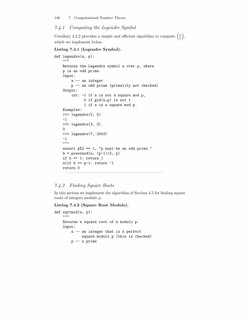
148 7. Computational Number Theory
7.4.1 Computing the Legendre Symbol
Corollary 4.2.2 provides a simple and efficient algorithm to compute(
ap
)
,
which we implement below.
Listing 7.4.1 (Legendre Symbol).
def legendre(a, p):
"""
Returns the Legendre symbol a over p, where
p is an odd prime.
Input:
a -- an integer
p -- an odd prime (primality not checked)
Output:
int: -1 if a is not a square mod p,
0 if gcd(a,p) is not 1
1 if a is a square mod p.
Examples:
>>> legendre(2, 5)
-1
>>> legendre(3, 3)
0
>>> legendre(7, 2003)
-1
"""
assert p%2 == 1, "p must be an odd prime."
b = powermod(a, (p-1)/2, p)
if b == 1: return 1
elif b == p-1: return -1
return 0
————————————————————————
7.4.2 Finding Square Roots
In this section we implement the algorithm of Section 4.5 for finding squareroots of integers modulo p.
Listing 7.4.2 (Square Root Modulo).
def sqrtmod(a, p):
"""
Returns a square root of a modulo p.
Input:
a -- an integer that is a perfect
square modulo p (this is checked)
p -- a prime
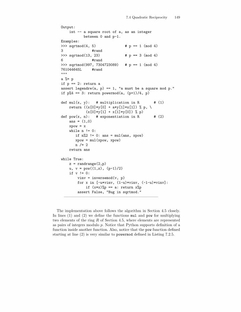
7.4 Quadratic Reciprocity 149
Output:
int -- a square root of a, as an integer
between 0 and p-1.
Examples:
>>> sqrtmod(4, 5) # p == 1 (mod 4)
3 #rand
>>> sqrtmod(13, 23) # p == 3 (mod 4)
6 #rand
>>> sqrtmod(997, 7304723089) # p == 1 (mod 4)
761044645L #rand
"""
a %= p
if p == 2: return a
assert legendre(a, p) == 1, "a must be a square mod p."
if p%4 == 3: return powermod(a, (p+1)/4, p)
def mul(x, y): # multiplication in R # (1)
return ((x[0]*y[0] + a*y[1]*x[1]) % p, \
(x[0]*y[1] + x[1]*y[0]) % p)
def pow(x, n): # exponentiation in R # (2)
ans = (1,0)
xpow = x
while n != 0:
if n%2 != 0: ans = mul(ans, xpow)
xpow = mul(xpow, xpow)
n /= 2
return ans
while True:
z = randrange(2,p)
u, v = pow((1,z), (p-1)/2)
if v != 0:
vinv = inversemod(v, p)
for x in [-u*vinv, (1-u)*vinv, (-1-u)*vinv]:
if (x*x)%p == a: return x%p
assert False, "Bug in sqrtmod."
————————————————————————
The implementation above follows the algorithm in Section 4.5 closely.In lines (1) and (2) we define the functions mul and pow for multiplyingtwo elements of the ring R of Section 4.5, where elements are representedas pairs of integers modulo p. Notice that Python supports definition of afunction inside another function. Also, notice that the pow function definedstarting at line (2) is very similar to powermod defined in Listing 7.2.5.
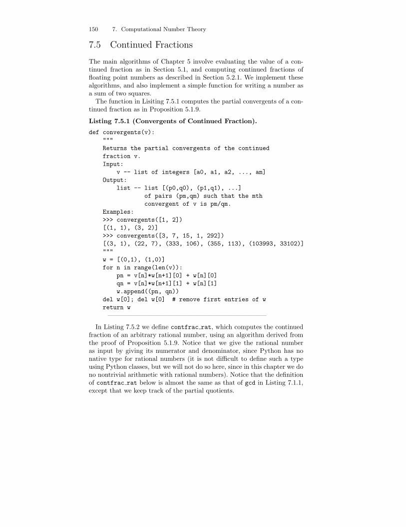
150 7. Computational Number Theory
7.5 Continued Fractions
The main algorithms of Chapter 5 involve evaluating the value of a con-tinued fraction as in Section 5.1, and computing continued fractions offloating point numbers as described in Section 5.2.1. We implement thesealgorithms, and also implement a simple function for writing a number asa sum of two squares.
The function in Lisiting 7.5.1 computes the partial convergents of a con-tinued fraction as in Proposition 5.1.9.
Listing 7.5.1 (Convergents of Continued Fraction).
def convergents(v):
"""
Returns the partial convergents of the continued
fraction v.
Input:
v -- list of integers [a0, a1, a2, ..., am]
Output:
list -- list [(p0,q0), (p1,q1), ...]
of pairs (pm,qm) such that the mth
convergent of v is pm/qm.
Examples:
>>> convergents([1, 2])
[(1, 1), (3, 2)]
>>> convergents([3, 7, 15, 1, 292])
[(3, 1), (22, 7), (333, 106), (355, 113), (103993, 33102)]
"""
w = [(0,1), (1,0)]
for n in range(len(v)):
pn = v[n]*w[n+1][0] + w[n][0]
qn = v[n]*w[n+1][1] + w[n][1]
w.append((pn, qn))
del w[0]; del w[0] # remove first entries of w
return w
————————————————————————
In Listing 7.5.2 we define contfrac rat, which computes the continuedfraction of an arbitrary rational number, using an algorithm derived fromthe proof of Proposition 5.1.9. Notice that we give the rational numberas input by giving its numerator and denominator, since Python has nonative type for rational numbers (it is not difficult to define such a typeusing Python classes, but we will not do so here, since in this chapter we dono nontrivial arithmetic with rational numbers). Notice that the definitionof contfrac rat below is almost the same as that of gcd in Listing 7.1.1,except that we keep track of the partial quotients.
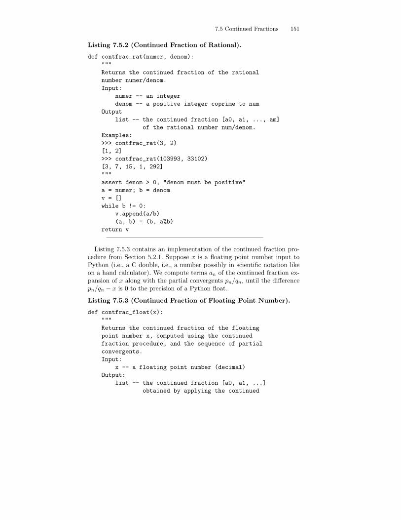
7.5 Continued Fractions 151
Listing 7.5.2 (Continued Fraction of Rational).
def contfrac_rat(numer, denom):
"""
Returns the continued fraction of the rational
number numer/denom.
Input:
numer -- an integer
denom -- a positive integer coprime to num
Output
list -- the continued fraction [a0, a1, ..., am]
of the rational number num/denom.
Examples:
>>> contfrac_rat(3, 2)
[1, 2]
>>> contfrac_rat(103993, 33102)
[3, 7, 15, 1, 292]
"""
assert denom > 0, "denom must be positive"
a = numer; b = denom
v = []
while b != 0:
v.append(a/b)
(a, b) = (b, a%b)
return v
————————————————————————
Listing 7.5.3 contains an implementation of the continued fraction pro-cedure from Section 5.2.1. Suppose x is a floating point number input toPython (i.e., a C double, i.e., a number possibly in scientific notation likeon a hand calculator). We compute terms an of the continued fraction ex-pansion of x along with the partial convergents pn/qn, until the differencepn/qn − x is 0 to the precision of a Python float.
Listing 7.5.3 (Continued Fraction of Floating Point Number).
def contfrac_float(x):
"""
Returns the continued fraction of the floating
point number x, computed using the continued
fraction procedure, and the sequence of partial
convergents.
Input:
x -- a floating point number (decimal)
Output:
list -- the continued fraction [a0, a1, ...]
obtained by applying the continued
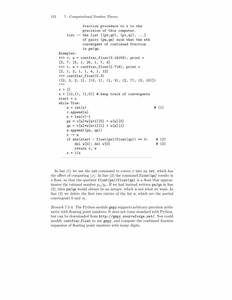
152 7. Computational Number Theory
fraction procedure to x to the
precision of this computer.
list -- the list [(p0,q0), (p1,q1), ...]
of pairs (pm,qm) such that the mth
convergent of continued fraction
is pm/qm.
Examples:
>>> v, w = contfrac_float(3.14159); print v
[3, 7, 15, 1, 25, 1, 7, 4]
>>> v, w = contfrac_float(2.718); print v
[2, 1, 2, 1, 1, 4, 1, 12]
>>> contfrac_float(0.3)
([0, 3, 2, 1], [(0, 1), (1, 3), (2, 7), (3, 10)])
"""
v = []
w = [(0,1), (1,0)] # keep track of convergents
start = x
while True:
a = int(x) # (1)
v.append(a)
n = len(v)-1
pn = v[n]*w[n+1][0] + w[n][0]
qn = v[n]*w[n+1][1] + w[n][1]
w.append((pn, qn))
x -= a
if abs(start - float(pn)/float(qn)) == 0: # (2)
del w[0]; del w[0] # (3)
return v, w
x = 1/x
————————————————————————
In line (1) we use the int command to coerce x into an int, which hasthe affect of computing ⌊x⌋. In line (2) the command float(qn) results ina float, so that the quotient float(pn)/float(qn) is a float that approx-imates the rational number pn/qn. If we had instead written pn/qn in line(2), then pn/qn would always be an integer, which is not what we want. Inline (3) we delete the first two entries of the list w, which are the partialconvergents 0 and ∞.
Remark 7.5.4. The Python module gmpy supports arbitrary precision arith-metic with floating point numbers. It does not come standard with Python,but can be downloaded from http://gmpy.sourceforge.net/. You couldmodify contfrac float to use gmpy, and compute the continued fractionexpansion of floating point numbers with many digits.
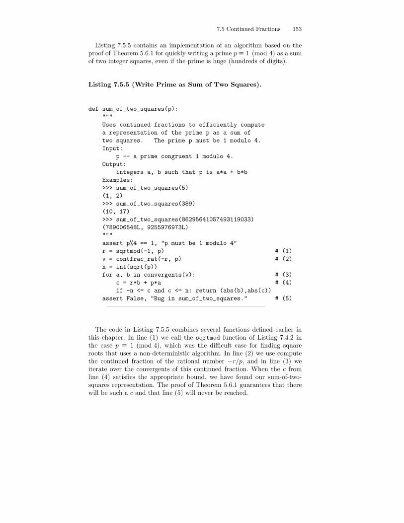
7.5 Continued Fractions 153
Listing 7.5.5 contains an implementation of an algorithm based on theproof of Theorem 5.6.1 for quickly writing a prime p ≡ 1 (mod 4) as a sumof two integer squares, even if the prime is huge (hundreds of digits).
Listing 7.5.5 (Write Prime as Sum of Two Squares).
def sum_of_two_squares(p):
"""
Uses continued fractions to efficiently compute
a representation of the prime p as a sum of
two squares. The prime p must be 1 modulo 4.
Input:
p -- a prime congruent 1 modulo 4.
Output:
integers a, b such that p is a*a + b*b
Examples:
>>> sum_of_two_squares(5)
(1, 2)
>>> sum_of_two_squares(389)
(10, 17)
>>> sum_of_two_squares(86295641057493119033)
(789006548L, 9255976973L)
"""
assert p%4 == 1, "p must be 1 modulo 4"
r = sqrtmod(-1, p) # (1)
v = contfrac_rat(-r, p) # (2)
n = int(sqrt(p))
for a, b in convergents(v): # (3)
c = r*b + p*a # (4)
if -n <= c and c <= n: return (abs(b),abs(c))
assert False, "Bug in sum_of_two_squares." # (5)
————————————————————————
The code in Listing 7.5.5 combines several functions defined earlier inthis chapter. In line (1) we call the sqrtmod function of Listing 7.4.2 inthe case p ≡ 1 (mod 4), which was the difficult case for finding squareroots that uses a non-deterministic algorithm. In line (2) we use computethe continued fraction of the rational number −r/p, and in line (3) weiterate over the convergents of this continued fraction. When the c fromline (4) satisfies the appropriate bound, we have found our sum-of-two-squares representation. The proof of Theorem 5.6.1 guarantees that therewill be such a c and that line (5) will never be reached.
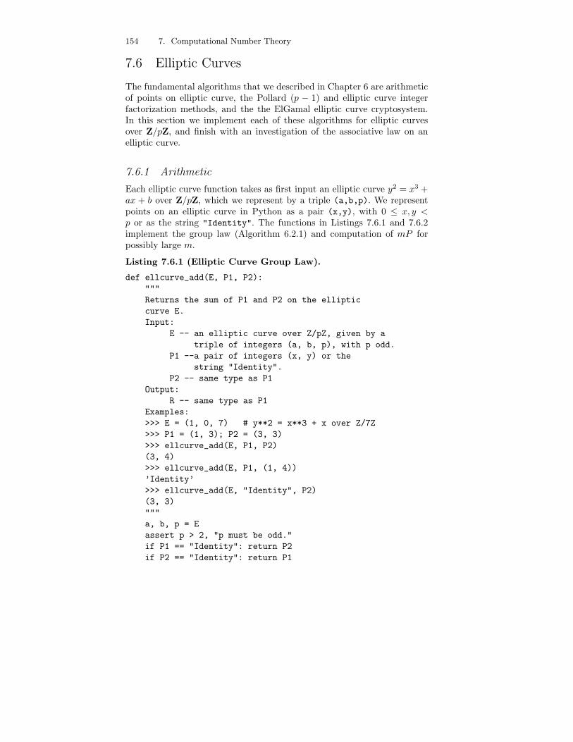
154 7. Computational Number Theory
7.6 Elliptic Curves
The fundamental algorithms that we described in Chapter 6 are arithmeticof points on elliptic curve, the Pollard (p − 1) and elliptic curve integerfactorization methods, and the the ElGamal elliptic curve cryptosystem.In this section we implement each of these algorithms for elliptic curvesover Z/pZ, and finish with an investigation of the associative law on anelliptic curve.
7.6.1 Arithmetic
Each elliptic curve function takes as first input an elliptic curve y2 = x3 +ax + b over Z/pZ, which we represent by a triple (a,b,p). We representpoints on an elliptic curve in Python as a pair (x,y), with 0 ≤ x, y <p or as the string "Identity". The functions in Listings 7.6.1 and 7.6.2implement the group law (Algorithm 6.2.1) and computation of mP forpossibly large m.
Listing 7.6.1 (Elliptic Curve Group Law).
def ellcurve_add(E, P1, P2):
"""
Returns the sum of P1 and P2 on the elliptic
curve E.
Input:
E -- an elliptic curve over Z/pZ, given by a
triple of integers (a, b, p), with p odd.
P1 --a pair of integers (x, y) or the
string "Identity".
P2 -- same type as P1
Output:
R -- same type as P1
Examples:
>>> E = (1, 0, 7) # y**2 = x**3 + x over Z/7Z
>>> P1 = (1, 3); P2 = (3, 3)
>>> ellcurve_add(E, P1, P2)
(3, 4)
>>> ellcurve_add(E, P1, (1, 4))
’Identity’
>>> ellcurve_add(E, "Identity", P2)
(3, 3)
"""
a, b, p = E
assert p > 2, "p must be odd."
if P1 == "Identity": return P2
if P2 == "Identity": return P1
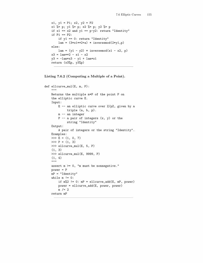
7.6 Elliptic Curves 155
x1, y1 = P1; x2, y2 = P2
x1 %= p; y1 %= p; x2 %= p; y2 %= p
if x1 == x2 and y1 == p-y2: return "Identity"
if P1 == P2:
if y1 == 0: return "Identity"
lam = (3*x1**2+a) * inversemod(2*y1,p)
else:
lam = (y1 - y2) * inversemod(x1 - x2, p)
x3 = lam**2 - x1 - x2
y3 = -lam*x3 - y1 + lam*x1
return (x3%p, y3%p)
————————————————————————
Listing 7.6.2 (Computing a Multiple of a Point).
def ellcurve_mul(E, m, P):
"""
Returns the multiple m*P of the point P on
the elliptic curve E.
Input:
E -- an elliptic curve over Z/pZ, given by a
triple (a, b, p).
m -- an integer
P -- a pair of integers (x, y) or the
string "Identity"
Output:
A pair of integers or the string "Identity".
Examples:
>>> E = (1, 0, 7)
>>> P = (1, 3)
>>> ellcurve_mul(E, 5, P)
(1, 3)
>>> ellcurve_mul(E, 9999, P)
(1, 4)
"""
assert m >= 0, "m must be nonnegative."
power = P
mP = "Identity"
while m != 0:
if m%2 != 0: mP = ellcurve_add(E, mP, power)
power = ellcurve_add(E, power, power)
m /= 2
return mP
————————————————————————
156 7. Computational Number Theory
7.6.2 Integer Factorization
In Listing 7.6.3 we implement Algorithm 6.3.2 for computing the leastcommon multiple of all integers up to some bound.
Listing 7.6.3 (Least Common Multiple of Numbers).
def lcm_to(B):
"""
Returns the least common multiple of all
integers up to B.
Input:
B -- an integer
Output:
an integer
Examples:
>>> lcm_to(5)
60
>>> lcm_to(20)
232792560
>>> lcm_to(100)
69720375229712477164533808935312303556800L
"""
ans = 1
logB = log(B)
for p in primes(B):
ans *= p**int(logB/log(p))
return ans
————————————————————————
Next we implement Pollard’s p − 1 method, as in Algorithm 6.3.3. Weuse only the bases a = 2, 3, but you could change this to use more basesby modifying the for loop in Listing 7.6.4.
Listing 7.6.4 (Pollard).
def pollard(N, m):
"""
Use Pollard’s (p-1)-method to try to find a
nontrivial divisor of N.
Input:
N -- a positive integer
m -- a positive integer, the least common
multiple of the integers up to some
bound, computed using lcm_to.
Output:
int -- an integer divisor of n
Examples:
7.6 Elliptic Curves 157
>>> pollard(5917, lcm_to(5))
61
>>> pollard(779167, lcm_to(5))
779167
>>> pollard(779167, lcm_to(15))
2003L
>>> pollard(187, lcm_to(15))
11
>>> n = random_prime(5)*random_prime(5)*random_prime(5)
>>> pollard(n, lcm_to(100))
315873129119929L #rand
>>> pollard(n, lcm_to(1000))
3672986071L #rand
"""
for a in [2, 3]:
x = powermod(a, m, N) - 1
g = gcd(x, N)
if g != 1 and g != N:
return g
return N
————————————————————————
In order to implement the elliptic curve method and also in our upcom-ing elliptic curve cryptography implementation, it will be useful to definethe function randcurve of Listing 7.6.5, which computes a random ellipticcurve over Z/pZ and a point on it. For simplicity, randcurve always re-turns a curve of the form y2 = x3 +ax+1, and the point P = (0, 1). As anexercise you could change this function to return a more general curve, andfind a random point by choosing a random x, then incrementing it untilx3 + ax + 1 is a perfect square.
Listing 7.6.5 (Random Elliptic Curve).
def randcurve(p):
"""
Construct a somewhat random elliptic curve
over Z/pZ and a random point on that curve.
Input:
p -- a positive integer
Output:
tuple -- a triple E = (a, b, p)
P -- a tuple (x,y) on E
Examples:
>>> p = random_prime(20); p
17758176404715800329L #rand
>>> E, P = randcurve(p)
>>> print E
158 7. Computational Number Theory
(15299007531923218813L, 1, 17758176404715800329L) #rand
>>> print P
(0, 1)
"""
assert p > 2, "p must be > 2."
a = randrange(p)
while gcd(4*a**3 + 27, p) != 1:
a = randrange(p)
return (a, 1, p), (0,1)
————————————————————————
In Listing 7.6.6, we implement the elliptic curve factorization method.
Listing 7.6.6 (Elliptic Curve Factorization Method).
def elliptic_curve_method(N, m, tries=5):
"""
Use the elliptic curve method to try to find a
nontrivial divisor of N.
Input:
N -- a positive integer
m -- a positive integer, the least common
multiple of the integers up to some
bound, computed using lcm_to.
tries -- a positive integer, the number of
different elliptic curves to try
Output:
int -- a divisor of n
Examples:
>>> elliptic_curve_method(5959, lcm_to(20))
59L #rand
>>> elliptic_curve_method(10007*20011, lcm_to(100))
10007L #rand
>>> p = random_prime(9); q = random_prime(9)
>>> n = p*q; n
117775675640754751L #rand
>>> elliptic_curve_method(n, lcm_to(100))
117775675640754751L #rand
>>> elliptic_curve_method(n, lcm_to(500))
117775675640754751L #rand
"""
for _ in range(tries): # (1)
E, P = randcurve(N) # (2)
try: # (3)
Q = ellcurve_mul(E, m, P) # (4)
except ZeroDivisionError, x: # (5)
g = gcd(x[0],N) # (6)
7.6 Elliptic Curves 159
if g != 1 or g != N: return g # (7)
return N
————————————————————————
In line (1) the underscore means that the for loop iterates tries times,but that no variable is “wasted” recording which iteration we are in. Inline (2) we compute a random elliptic curve and point on it. The ellipticcurve method works by assuming N is prime, doing a certain computation,on an elliptic curve over Z/NZ, and detecting if something goes wrong.Python contains a mechanism called exception handling, which leads toa very simple implementation of the elliptic curve method, that uses theelliptic curve functions that we have already defined. The try statementin line (3) means that the code in line (4) should be executed, and if theZeroDivisionError exception is raised, then the code in lines (6) and(7) should be executed, but not otherwise. Recall that in the definition ofinversemod from Listing 7.2.2, when the inverse could not be computed,we raised a ZeroDivisionError, which included the offending pair (a, n).Thus when computing mP , if at any point it is not possible to inverta number modulo N , we jump to line (6), compute a gcd with N , andhopefully split N .
7.6.3 ElGamal Elliptic Curve Cryptosystem
Listing 7.6.7 defines a function that creates an ElGamal cryptosystem overZ/pZ. This is simplified from what one would do in actual practice. Onewould use a more general random elliptic curve and point than we do inelgamal init, and count the number of points on it using the Schoof-Elkies-Atkin algorithm, then repeat this procedure if the number of pointsis not a prime or a prime times a small number, or is p, p − 1, or p + 1.Since implementing Schoof-Elkies-Atkin is beyond the scope of this book,we have not included this crucial step.
Listing 7.6.7 (Initialize ElGamal).
def elgamal_init(p):
"""
Constructs an ElGamal cryptosystem over Z/pZ, by
choosing a random elliptic curve E over Z/pZ, a
point B in E(Z/pZ), and a random integer n. This
function returns the public key as a 4-tuple
(E, B, n*B) and the private key n.
Input:
p -- a prime number
Output:
tuple -- the public key as a 3-tuple
(E, B, n*B), where E = (a, b, p) is an
160 7. Computational Number Theory
elliptic curve over Z/pZ, B = (x, y) is
a point on E, and n*B = (x’,y’) is
the sum of B with itself n times.
int -- the private key, which is the pair (E, n)
Examples:
>>> p = random_prime(20); p
17758176404715800329L #rand
>>> public, private = elgamal_init(p)
>>> print "E =", public[0]
E = (15299007531923218813L, 1, 17758176404715800329L) #rand
>>> print "B =", public[1]
B = (0, 1)
>>> print "nB =", public[2]
nB = (5619048157825840473L, 151469105238517573L) #rand
>>> print "n =", private[1]
n = 12608319787599446459 #rand
"""
E, B = randcurve(p)
n = randrange(2,p)
nB = ellcurve_mul(E, n, B)
return (E, B, nB), (E, n)
————————————————————————
In Listing 7.6.8 we define elgamal encrypt, which encrypts a messageusing the ElGamal cryptosystem on an elliptic curve.
Listing 7.6.8 (Encrypt Using ElGamal).
def elgamal_encrypt(plain_text, public_key):
"""
Encrypt a message using the ElGamal cryptosystem
with given public_key = (E, B, n*B).
Input:
plain_text -- a string
public_key -- a triple (E, B, n*B), as output
by elgamal_init.
Output:
list -- a list of pairs of points on E that
represent the encrypted message
Examples:
>>> public, private = elgamal_init(random_prime(20))
>>> elgamal_encrypt("RUN", public)
[((6004308617723068486L, 15578511190582849677L), \ #rand
(7064405129585539806L, 8318592816457841619L))] #rand
"""
E, B, nB = public_key
a, b, p = E
7.6 Elliptic Curves 161
assert p > 10000, "p must be at least 10000."
v = [1000*x for x in \
str_to_numlist(plain_text, p/1000)] # (1)
cipher = []
for x in v:
while not legendre(x**3+a*x+b, p)==1: # (2)
x = (x+1)%p
y = sqrtmod(x**3+a*x+b, p) # (3)
P = (x,y)
r = randrange(1,p)
encrypted = (ellcurve_mul(E, r, B), \
ellcurve_add(E, P, ellcurve_mul(E,r,nB)))
cipher.append(encrypted)
return cipher
————————————————————————
In line (1) we encode the plain text message as a sequence of integersthat are all 0 modulo 1000. It would be nice if the integers returned bystr to numlist were the x-coordinates of points on the elliptic curve E,but typically only half the x ∈ Z/pZ will actually be x-coordinates of pointson E. Thus we multiply the integers returned by str to numlist, and 1to them in line (2) until they are the x-coordinates of points on E. Notethat since half the elements of Z/pZ are perfect squares, we should onlyhave to add 1 very few times to obtain a perfect square. The rest of theListing 7.6.8 is a straightforward implementation of ElGamal as describedin Section 6.4.2.
In Listing 7.6.9 we give the corresponding decryption routine, which takesinto account the way we encoded integers as points on E.
Listing 7.6.9 (Decrypt Using ElGamal).
def elgamal_decrypt(cipher_text, private_key):
"""
Encrypt a message using the ElGamal cryptosystem
with given public_key = (E, B, n*B).
Input:
cipher_text -- list of pairs of points on E output
by elgamal_encrypt.
Output:
str -- the unencrypted plain text
Examples:
>>> public, private = elgamal_init(random_prime(20))
>>> v = elgamal_encrypt("TOP SECRET MESSAGE!", public)
>>> print elgamal_decrypt(v, private)
TOP SECRET MESSAGE!
"""
E, n = private_key
162 7. Computational Number Theory
p = E[2]
plain = []
for rB, P_plus_rnB in cipher_text:
nrB = ellcurve_mul(E, n, rB)
minus_nrB = (nrB[0], -nrB[1])
P = ellcurve_add(E, minus_nrB, P_plus_rnB)
plain.append(P[0]/1000)
return numlist_to_str(plain, p/1000)
————————————————————————
7.7 Exercises
7.1 (a) Let y = 10000. Compute π(y) = #{primes p ≤ y}.(b) The prime number theorem implies π(x) is asymptotic to x
log(x) .
How close is π(y) to y/ log(y), where y is as in (a)?
7.2 Design an analogue of the trial division function of Listing 7.1.3that uses a sequence dif of length longer than 8, so it skips integersnot coprime to 210 (see the discussion after Listing 7.1.3).
7.3 Compute the last two digits of 345.
7.4 Find the integer a such that 0 ≤ a < 113 and
10270 + 1 ≡ a37 (mod 113).
7.5 Find the proportion of primes p < 1000 such that 2 is a primitiveroot modulo p.
7.6 Find a prime p such that the smallest primitive root modulo p is 37.
7.7 You and Nikita wish to agree on a secret key using the Diffie-Hellmankey exchange. Nikita announces that p = 3793 and g = 7. Nikitasecretly chooses a number n < p and tells you that gn ≡ 454 (mod p).You choose the random number m = 1208. What is the secret key?
7.8 You see Michael and Nikita agree on a secret key using the Diffie-Hellman key exchange. Michael and Nikita choose p = 97 and g = 5.Nikita chooses a random number n and tells Michael that gn ≡ 3(mod 97), and Michael chooses a random number m and tells Nikitathat gm ≡ 7 (mod 97). Brute force crack their code: What is thesecret key that Nikita and Michael agree upon? What is n? Whatis m?
7.9 In this problem, you will “crack” an RSA cryptosystem. What is thesecret decoding number d for the RSA cryptosystem with public key(n, e) = (5352381469067, 4240501142039)?
7.7 Exercises 163
7.10 Nikita creates an RSA cryptosystem with public key
(n, e) = (1433811615146881, 329222149569169).
In the following two problems, show the steps you take to factor n.(Don’t simply factor n directly using a computer.)
(a) Somehow you discover that d = 116439879930113. Show howto use the probabilistic algorithm of Section 3.3.3 to use d tofactor n.
(b) In part (a) you found that the factors p and q of n are veryclose. Show how to use the Fermat factorization method of Sec-tion 3.3.2 to factor n.
7.11 Compute the pn and qn for the continued fractions [−3, 1, 1, 1, 1, 3]and [0, 2, 4, 1, 8, 2]. Check that the propositions in Section 5.1.1 hold.
7.12 A theorem of Hurwitz (1891) asserts that for any irrational number x,there exists infinitely many rational numbers a/b such that
∣
∣
∣x − a
b
∣
∣
∣<
1√5b2
.
Take x = e, and obtain four rational numbers that satisfy this in-equality.
7.13 Which of the following numbers is a sum of two squares? Expressthose that are as a sum of two squares.
−389, 12345, 729, 1729, 5809961789
7.14 (a) Show that the set of numbers 59 + 1 ± s for s ≤ 15 contains 14numbers that are B-power smooth for B = 20.
(b) Find the proportion of primes p in the interval from 1012 and1012 + 1000 such that p − 1 is B = 105 power-smooth.
164 7. Computational Number Theory
This is page 165Printer: Opaque this
Answers and Hints
1. Prime Numbers
2. They are 2, 3, 5, 7, 11, 13, 17, 19, 23, 29, 31, 37, 41, 43, 47, 53, 59,61, 67, 71, 73, 79, 83, 89, 97.
3. Emulate the proof of Proposition 1.2.4.
2. The Ring of Integers Modulo n
1. They are 5, 13, 3, and 8.
2. For example x = 22, y = −39.
3. Hint: Use the binomial theorem and prove that if r ≥ 1 then pdivides
(
pr
)
.
6. For example, S1 = {0, 1, 2, 3, 4, 5, 6}, S2 = {1, 3, 5, 7, 11, 13, 23},S3 = {0, 2, 4, 6, 8, 10, 12}, and S4 = {2, 3, 5, 7, 11, 13, 29}. In eachwe find Si by listing the first seven numbers satisfying the ithcondition, then adjusted the last number if necessary so that thereductions would be distinct modulo 7.
7. An integer is divisible by 5 if and only if the last digits is 0 or 5.An integer is divisible by 9 if and only if the sum of the digitsis divisible by 9. An integer is divisible by 11 if and only if thealternating sum of the digits is divisible by 11.
8. Hint for part (a): Use the divisibility rule you found in Exer-cise 1.7.
166 7. Computational Number Theory
9. 71
10. 8
11. As explained on page 22, we know that Z/nZ is a ring for any n.Thus to show that Z/pZ is a field it suffices to show that everynonzero element a ∈ Z/pZ has an inverse. Lift a to an elementa ∈ Z, and set b = p in Proposition 2.3.1. Because p is prime,gcd(a, p) = 1, so there exists x, y such that ax+py = 1. Reducingthis equality modulo p proves that a has an inverse x (mod p).Alternative one could argue just like after Definition 2.1.10 thatam = 1 for some m, so some power of a is the inverse of a.
12. 302
14. Only for n = 1, 2. If n > 2, then n is either divisible by anodd prime p or 4. If 4 | n, then 2e − 2e−1 divides ϕ(n) for somee ≥ 2, so ϕ(n) is even. If an odd p divides n, then the evennumber pe − pe−1 divides ϕ(n) for some e ≥ 1.
15. The map ψ is a homomorphism since both reduction maps
Z/mnZ → Z/mZ and Z/mnZ → Z/nZ
are homomorphisms. It is injective because if a ∈ Z is such thatψ(a) = 0, then m | a and n | a, so mn | a (since m and n arecoprime), so a ≡ 0 (mod mn). The cardinality of Z/mnZ is mnand the cardinality of the product Z/mZ × Z/nZ is also mn,so ψ must be an isomorphism. The units (Z/mnZ)∗ are thus inbijection with the units (Z/mZ)∗ × (Z/nZ)∗.
For the second part of the exercise, let g = gcd(m,n) and seta = mn/g. Then a 6≡ 0 (mod mn), but m | a and n | a, soa ker(ψ).
16. We express the question as a system of linear equations modulovarious numbers, and use the Chinese remainder theorem. Letx be the number of books. The problem asserts that
x ≡ 6 (mod 7)
x ≡ 2 (mod 6)
x ≡ 1 (mod 5)
x ≡ 0 (mod 4)
Applying CRT to the first pair of equations we find that x ≡ 20(mod 42). Applying CRT to this equation and the third we findthat x ≡ 146 (mod 210). Since 146 is not divisible by 4, we addmultiples of 210 to 146 until we find the first x that is divisibleby 4. The first multiple works, and we find that the aspiringmathematicians have 356 math books.
7.7 Exercises 167
17. Note that p = 3 works, since 11 = 32 + 2 is prime. Now supposep 6= is any prime such that p and p2+2 are both prime. We musthave p ≡ 1 (mod 3) or p ≡ 2 (mod 3). Then p2 ≡ 1 (mod 3),so p2 + 2 ≡ 0 (mod 3), which contradicts the fact that p2 + 2 isprime.
18. For (a) n = 1, 2, see solution to Exercise 2.14. For (b), yes thereare many such examples. For example, m = 2, n = 4.
19. By repeated application of multiplicativity and Equation (2.2.2)on page 29, we see that if n =
∏
i pei
i is the prime factorizationof n, then
ϕ(n) =∏
i
(pei
i − pei−1i ) =
∏
i
pei−1i ·
∏
i
(pi − 1).
20. 1, 6, 29, 34
21. Let g = gcd(12n+1, 30n+2). Then g | 30n+2−2·(12n+1) = 6n.For the same reason g also divides 12n+1−2·(6n) = 1, so g = 1,as claimed.
24. There is no primitive root modulo 8, since (Z/8Z)∗ has order4, but every element of (Z/8Z)∗ has order 2. Prove that if ζ isa primitive root modulo 2n, for n ≥ 3, then the reduction of ζmod 8 is a primitive root, a contradiction.
25. 2 is a primitive root modulo 125.
26. Let∏m
i=1 pei
i be the prime factorization of n. Slightly generaliz-ing Exercise 15 we see that
(Z/nZ)∗ ∼=∏
(Z/pei
i Z)∗.
Thus (Z/nZ)∗ is cyclic if and only if the product (Z/pei
i Z)∗ iscyclic. If 8 | n, then there is no chance (Z/nZ)∗ is cyclic, soassume 8 ∤ n. Then by Exercise 2.25 each group (Z/pei
i Z)∗ isitself cyclic. A product of cyclic groups is cyclic if and only theorders of the factors in the product are coprime (this follows fromExercise 2.15). Thus (Z/nZ)∗ is cyclic if and only if the numberspi(pi − 1), for i = 1, . . . ,m are pairwise coprime. Since pi − 1 iseven, there can be at most one odd prime in the factorization ofn, and we see that (Z/nZ)∗ is cyclic if and only if n is an oddprime power, twice an odd prime power, or n = 4.
3. Public-Key Cryptography
1. The best case is that each letter is A. Then the question is to findthe largest n such that 1 + 27 + · · ·+ 27n ≤ 1020. By computing
168 7. Computational Number Theory
log27(1020), we see that 2713 < 1020 and 2714 > 1020. Thusn ≤ 13, and since 1+27+ · · ·+27n−1 < 27n, and 2 ·2713 < 1020,it follows that n = 13.
2. This is not secure, since it is just equivalent to a “Ceaser Ci-pher”, that is a permutation of the letters of the alphabet, whichis well-known to be easily broken using a frequency analysis.
3. If we can compute the polynomial
f = (x−p)(x−q)(x−r) = x3−(p+q+r)x2+(pq+pr+qr)x−pqr,
then we can factor n by finding the roots of f , e.g., using New-ton’s method (or Cardona’s formula for the roots of a cubic).Because p, q, r, are distinct odd primes we have
ϕ(n) = (p − 1)(q − 1)(r − 1) = pqr − (pq + pr + qr) + p + q + r,
andσ(n) = 1 + (p + q + r) + (pq + pr + qr) + pqr.
Since we know n, ϕ(n), and σ(n), we know
σ(n) − 1 − n = (p + q + r) + (pq + pr + qr), and
ϕ(n) − n = (p + q + r) − (pq + pr + qr).
We can thus compute both p + q + r and pq + pr + qr, hencededuce f and find p, q, r.
4. Quadratic Reciprocity
1. They are all 1, −1, 0, and 1.
2. By Proposition 4.3.3 the value of(
3p
)
depends only on the re-
duction ±p (mod 12). List enough primes p such that the ±preduce to 1, 5, 7, 11 modulo 12 and verify that the asserted for-mula holds for each of them.
6. Since p = 213 − 1 is prime there are either two solutions or nosolutions to x2 ≡ 5 (mod p), and we can decide which usingquadratic reciprocity. We have
(
5
p
)
= (−1)(p−1)/2·(5−1)/2(p
5
)
=(p
5
)
,
so there are two solutions if and only if p = 213 −1 is ±1 mod 5.In fact p ≡ 1 (mod 5), so there are two solutions.
7. We have 448 = 296. By Fermat’s Little Theorem 296 = 1, sox = 1.
7.7 Exercises 169
8. For (a) take a = 19 and n = 20. We found this example us-ing the Chinese remainder theorem applied to 4 (mod 5) and 3(mod 4), and used that
(
1920
)
=(
195
)
·(
194
)
= (−1)(−1) = 1, yet19 is not a square modulo either 5 or 4, so is certainly not asquare modulo 20.
9. Hint: First reduce to the case that 6k − 1 is prime, by usingthat if p and q are primes not of the form 6k − 1, then neitheris their product. If p = 6k − 1 divides n2 + n + 1, it divides4n2 + 4n + 4 = (2n + 1)2 + 3, so −3 is a quadratic residuemodulo p. Now use quadratic reciprocity to show that −3 is nota quadratic residue modulo p.
5. Continued Fractions
9. Suppose n = x2 + y2, with x, y ∈ Q. Let d be such that dx, dy ∈Z. Then d2n = (dx)2 + (dy)2 is a sum of two integer squares, soby Theorem 5.6.1 if p | d2n and p ≡ 3 (mod 4), then ordp(d
2n)is even. We have ordp(d
2n) is even if and only if ordp(n) is even,so Theorem 5.6.1 implies that n is also a sum of two squares.
11. The squares modulo 8 are 0, 1, 4, so a sum of two squares reducesmodulo 8 to one of 0, 1, 2, 4 or 5. Four consecutive integers thatare sums of squares would reduce to four consecutive integers inthe set {0, 1, 2, 4, 5}, which is impossible.
6. Elliptic Curves
2. The second point of intersection is (129/100, 383/1000).
3. The group is cyclic of order 9, generated by (4, 2). The elementsof E(K) are
{O, (4, 2), (3, 4), (2, 4), (0, 4), (0, 1), (2, 1), (3, 1), (4, 3)}.
4. In part (a) the pattern is that Np = p + 1. For part (b), a hintis that when p ≡ 2 (mod 3), the map x 7→ x3 on (Z/pZ)∗ is anautomorphism, so x 7→ x3 + 1 is a bijection. Now use what youlearned about squares in Z/pZ from Chapter 4.
5. For all sufficiently large real x, the equation y2 = x3 +ax+b hasa real solution y. Thus the group E(R) is not countable, since Ris not countable. But any finitely generated group is countable.
6. In a course on abstract algebra one often proves the nontrivialfact that every subgroup of a finitely generated abelian groupis finitely generated. In particular, the torsion subgroup Gtor isfinitely generated. However, a finitely generated abelian torsiongroup is finite.
170 7. Computational Number Theory
7. Hint: Multiply both sides of y2 = x3 + ax + b by a power of acommon denominator, and “absorb” powers into x and y.
8. Hint: see Exercise 4.5.
7. Computational Number TheoryAll code below assume that the Python functions from Chapter 7have been defined.
1. >>> len(primes(10000))
1229
>>> 10000/log(10000)
1085.73620476
3. >>> powermod(3,45,100)
43
4. First raise both sides of the equation to the power of the multi-plicative inverse of 37 modulo 112 = ϕ(113), which is 109 to geta ≡ (10270 +1)109 (mod 113). We then evaluate this and obtaina = 60.
>>> inversemod(37, 112)
109
>>> powermod(102, 70, 113)
98
>>> powermod(99, 109, 113)
60
5. Using the following program we see that the number 2 is a prim-itive root 67 out of 168 times (about 40 percent).
>>> P = primes(1000)
>>> Q = [p for p in P if primitive_root(p) == 2]
>>> print len(Q), len(P)
67 168
6. The first such prime is 36721.
>>> P = primes(50000)
>>> Q = [primitive_root(p) for p in P]
>>> Q.index(37)
3893
>>> P[3893]
36721
7. 2156, since the secret key is gnm ≡ 454m ≡ 2156.
7.7 Exercises 171
8. To break the system, we need to find n such that 5n ≡ 3(mod 97). The following program does this finds n = 70, andsimilarly one finds that m = 31. The secret key is 570·31 ≡ 44(mod 97).
>>> for n in range(97):
... if powermod(5,n,97)==3: print n
70
9. We factor n and computer ϕ(n) then the inverse d of e moduloϕ(n).
>>> factor(5352381469067)
[(141307, 1), (37877681L, 1)]
>>> d=inversemod(4240501142039, (141307-1)*(37877681-1))
>>> d
5195621988839L
11. >>> convergents([-3,1,1,1,1,3])
[(-3, 1), (-2, 1), (-5, 2), (-7, 3), \
(-12, 5), (-43, 18)]
>>> convergents([0,2,4,1,8,2])
[(0, 1), (1, 2), (4, 9), (5, 11), \
(44, 97), (93, 205)]
12. The following code outputs the first 8 examples. First we importthe math library, in order to compute a decimal approximationto e. Then we compute terms of the continued fraction of e alongwith the partial convergents. Finally we print only those partialconvergents that satisfy the Hurwitz inequality.
>>> import math
>>> e = math.exp(1)
>>> v, convs = contfrac_float(e)
>>> [(a,b) for a, b in convs if \
abs(e - a*1.0/b) < 1/(math.sqrt(5)*b**2)]
[(3, 1), (19, 7), (193, 71), (2721, 1001),\
(49171, 18089), (1084483, 398959),\
(28245729, 10391023), (325368125, 119696244)]
13. −389 is not a sum of two squares because it is negative. 12345is not because 3 exactly divides it. 729 = 36 = (33)2 + 02. Thenumber 5809961789 is prime and equals 515422 + 561552.
>>> factor(12345)
[(3, 1), (5, 1), (823, 1)]
>>> factor(729)
[(3, 6)]
>>> factor(5809961789)
172 7. Computational Number Theory
[(5809961789L, 1)]
>>> 5809961789 % 4
1L
>>> sum_of_two_squares(5809961789)
(51542L, 56155L)
14. We use the following program. The computation of Ps takes afew seconds, since our implementation of factor is not veryefficient.
>>> N = [60 + s for s in range(-15,16)]
>>> def is_powersmooth(B, x):
... for p, e in factor(x):
... if p**e > B: return False
... return True
>>> Ns = [x for x in N if is_powersmooth(20, x)]
>>> print len(Ns), len(N), len(Ns)*1.0/len(N)
14 31 0.451612903226
>>> P = [x for x in range(10**12, 10**12+1000)\
if miller_rabin(x)]
>>> Ps = [x for x in P if \
is_powersmooth(10000, x-1)]
>>> print len(Ps), len(P), len(Ps)*1.0/len(P)
2 37 0.0540540540541
This is page 173Printer: Opaque this
References
[ACD+99] K. Aardal, S. Cavallar, B. Dodson, A. Lenstra, W. Lioen, P. L.Montgomery, B. Murphy, J. Gilchrist, G. Guillerm, P. Leyland,J. Marchand, F. Morain, A. Muffett, C.&C. Putnam, and P. Zim-mermann, Factorization of a 512-bit RSA key using the NumberField Sieve, http://www.loria.fr/~zimmerma/records/RSA155(1999).
[AGP94] W. R. Alford, Andrew Granville, and Carl Pomerance, Thereare infinitely many Carmichael numbers, Ann. of Math. (2) 139(1994), no. 3, 703–722. MR 95k:11114
[AKS02] M. Agrawal, N. Kayal, and N. Saxena, PRIMES is in P , toappear in Annals of Math.,http://www.cse.iitk.ac.in/users/manindra/primality.ps
(2002).
[BS76] Leonard E. Baum and Melvin M. Sweet, Continued fractions ofalgebraic power series in characteristic 2, Ann. of Math. (2) 103(1976), no. 3, 593–610. MR 53 #13127
[Bur89] D. M. Burton, Elementary number theory, second ed., W. C.Brown Publishers, Dubuque, IA, 1989. MR 90e:11001
[Cal] C. Caldwell, The Largest Known Primes,http://www.utm.edu/research/primes/largest.html.
174 References
[Cer] Certicom, The certicom ECC challenge,http://www.certicom.com/
index.php?action=res,ecc challenge.
[Cla] Clay Mathematics Institute, Millennium prize problems,http://www.claymath.org/millennium prize problems/.
[Coh] H. Cohn, A short proof of the continued fraction expansion of e,http://research.microsoft.com/~cohn/publications.html.
[Coh93] H. Cohen, A course in computational algebraic number theory,Graduate Texts in Mathematics, vol. 138, Springer-Verlag, Berlin,1993. MR 94i:11105
[Con97] John H. Conway, The sensual (quadratic) form, Carus Mathemat-ical Monographs, vol. 26, Mathematical Association of America,Washington, DC, 1997, With the assistance of Francis Y. C. Fung.MR 98k:11035
[CP01] R. Crandall and C. Pomerance, Prime numbers, Springer-Verlag,New York, 2001, A computational perspective. MR 2002a:11007
[Cre] J. E. Cremona, mwrank (computer software),http://www.maths.nott.ac.uk/personal/jec/ftp/progs/.
[Cre97] , Algorithms for modular elliptic curves, second ed., Cam-bridge University Press, Cambridge, 1997.
[Dav99] H. Davenport, The higher arithmetic, seventh ed., Cambridge Uni-versity Press, Cambridge, 1999, An introduction to the theory ofnumbers, Chapter VIII by J. H. Davenport. MR 2000k:11002
[DH76] W. Diffie and M.E. Hellman, New directions in cryptography,IEEE Trans. Information Theory IT-22 (1976), no. 6, 644–654.MR 55 #10141
[Eul85] Leonhard Euler, An essay on continued fractions, Math. SystemsTheory 18 (1985), no. 4, 295–328, Translated from the Latin byB. F. Wyman and M. F. Wyman. MR 87d:01011b
[FT93] A. Frohlich and M. J. Taylor, Algebraic number theory, CambridgeUniversity Press, Cambridge, 1993. MR 94d:11078
[GS02] X. Gourdon and P. Sebah, The π(x) project,http://numbers.computation.free.fr/constants/primes/
pix/pixproject.html.
[Guy94] R. K. Guy, Unsolved problems in number theory, second ed.,Springer-Verlag, New York, 1994, Unsolved Problems in IntuitiveMathematics, I. MR 96e:11002
References 175
[Har77] R. Hartshorne, Algebraic Geometry, Springer-Verlag, New York,1977, Graduate Texts in Mathematics, No. 52.
[Hoo67] C. Hooley, On Artin’s conjecture, J. Reine Angew. Math. 225(1967), 209–220. MR 34 #7445
[HW79] G. H. Hardy and E. M. Wright, An introduction to the theory ofnumbers, fifth ed., The Clarendon Press Oxford University Press,New York, 1979. MR 81i:10002
[IBM01] IBM, IBM’s Test-Tube Quantum Computer Makes History,http://www.research.ibm.com/resources/news/
20011219 quantum.shtml.
[IR90] K. Ireland and M. Rosen, A classical introduction to modernnumber theory, second ed., Springer-Verlag, New York, 1990. MR92e:11001
[Khi63] A. Ya. Khintchine, Continued fractions, Translated by PeterWynn, P. Noordhoff Ltd., Groningen, 1963. MR 28 #5038
[Knu97] Donald E. Knuth, The art of computer programming, thirded., Addison-Wesley Publishing Co., Reading, Mass.-London-Amsterdam, 1997, Volume 1: Fundamental algorithms, Addison-Wesley Series in Computer Science and Information Processing.
[Knu98] , The art of computer programming. Vol. 2, second ed.,Addison-Wesley Publishing Co., Reading, Mass., 1998, Seminu-merical algorithms, Addison-Wesley Series in Computer Scienceand Information Processing. MR 83i:68003
[Kob84] N. Koblitz, Introduction to elliptic curves and modular forms,Graduate Texts in Mathematics, vol. 97, Springer-Verlag, NewYork, 1984. MR 86c:11040
[Leh14] D. N. Lehmer, List of primes numbers from 1 to 10,006,721,Carnegie Institution Washington, D.C. (1914).
[Lem] F. Lemmermeyer, Proofs of the Quadratic Reciprocity Law,http://www.rzuser.uni-heidelberg.de/~hb3/rchrono.html.
[Len87] H. W. Lenstra, Jr., Factoring integers with elliptic curves, Ann.of Math. (2) 126 (1987), no. 3, 649–673. MR 89g:11125
[LL93] A. K. Lenstra and H. W. Lenstra, Jr. (eds.), The development ofthe number field sieve, Lecture Notes in Mathematics, vol. 1554,Springer-Verlag, Berlin, 1993. MR 96m:11116
176 References
[LMG+01] Vandersypen L. M., Steffen M., Breyta G., Yannoni C. S., Sher-wood M. H., and Chuang I. L., Experimental realization of Shor’squantum factoring algorithm using nuclear magnetic resonance,Nature 414 (2001), no. 6866, 883–887.
[LT72] S. Lang and H. Trotter, Continued fractions for some algebraicnumbers, J. Reine Angew. Math. 255 (1972), 112–134; addendum,ibid. 267 (1974), 219–220; MR 50 #2086. MR 46 #5258
[LT74] , Addendum to: “Continued fractions for some algebraicnumbers” (J. Reine Angew. Math. 255 (1972), 112–134), J. ReineAngew. Math. 267 (1974), 219–220. MR 50 #2086
[Mor93] P. Moree, A note on Artin’s conjecture, Simon Stevin 67 (1993),no. 3-4, 255–257. MR 95e:11106
[NZM91] I. Niven, H. S. Zuckerman, and H. L. Montgomery, An introduc-tion to the theory of numbers, fifth ed., John Wiley & Sons Inc.,New York, 1991. MR 91i:11001
[Old70] C. D. Olds, The Simple Continued Fraction Expression of e, Amer.Math. Monthly 77 (1970), 968–974.
[Per57] O. Perron, Die Lehre von den Kettenbruchen. Dritte, verbesserteund erweiterte Aufl. Bd. II. Analytisch-funktionentheoretischeKettenbruche, B. G. Teubner Verlagsgesellschaft, Stuttgart, 1957.MR 19,25c
[Ros] Guido van Rossum, Python,http://www.python.org.
[RSA] RSA, The New RSA Factoring Challenge,http://www.rsasecurity.com/rsalabs/challenges/factoring.
[RSA78] R. L. Rivest, A. Shamir, and L. Adleman, A method for obtainingdigital signatures and public-key cryptosystems, Comm. ACM 21(1978), no. 2, 120–126. MR 83m:94003
[Sho97] P. W. Shor, Polynomial-time algorithms for prime factorizationand discrete logarithms on a quantum computer, SIAM J. Com-put. 26 (1997), no. 5, 1484–1509. MR 98i:11108
[Sil86] J. H. Silverman, The arithmetic of elliptic curves, Graduate Textsin Mathematics, vol. 106, Springer-Verlag, New York, 1986. MR87g:11070
[Sin99] S. Singh, The Code Book: The Science of Secrecy from AncientEgypt to Quantum Cryptography, Doubleday, 1999.
References 177
[Slo] N. J. A. Sloane, The On-Line Encyclopedia of Integer Sequences,http://www.research.att.com/~njas/sequences/.
[ST92] J. H. Silverman and J. Tate, Rational points on elliptic curves, Un-dergraduate Texts in Mathematics, Springer-Verlag, New York,1992. MR 93g:11003
[Wal48] H. S. Wall, Analytic Theory of Continued Fractions, D. Van Nos-trand Company, Inc., New York, N. Y., 1948. MR 10,32d
[Wei03] E. W. Weisstein, RSA-576 Factored,http://mathworld.wolfram.com/news/2003-12-05/rsa/.
[Wil00] A. J. Wiles, The Birch and Swinnerton-Dyer Conjecture,http://www.claymath.org/prize problems/birchsd.htm.
[Zag75] D. Zagier, The first 50 million prime numbers,http://modular.fas.harvard.edu/scans/papers/zagier/.


