
Page--955
Energy use and production, demography and the world-marketoil price influencing twenty years of economic performance
and environmental degradation in Mexico
Luis G. López LemusH
State University of New YorkCollege of Environmental Science & ForestryOne Forestry Drive- 304 Illick HallSyracuse, New York 13210-2778USA
AbstractI present a compilation of data describing Mexico’s economic performance as it relates to demographic,and natural resource characteristics. Statistical correlations suggest that long term economic output andenergy efficiency are determined mostly by human population numbers and the fossil fuel consumptionrate. Significant relations were also found in the rates of deforestation, air pollution and agriculturalproduction, being all of these variables seemingly independent of a decreasing human population growthrate. The observed fluctuations were clearly driven by those of the world-market oil price throughout 1970-90. Neither energy production, agricultural yield, OPEC’s oil price or forest coverage appeared asimportant in determining Mexican GDP response for this 20-year period. The multi-factor statistical modelderived from the analyses of these trends casts serious concerns on present and future energy needs, socialdevelopment perspectives and the environment. Finally, as the country drives its transition into a sustainabledevelopment economy, in the midst of NAFTA and some other globalization trends, I discuss —from thissystems/energy perspective, how Mexico could bridge the GDP gap with its current NAFTA partners. Thejudicious use of its fossil fuel reserves, along with the management of energy-related environmentalproblems, and the reorientation of its growth efforts towards the direct [sustainable] exploitation of its solar-based resources, are considered within this context. Whether emphasis is placed on agriculture, fisheries,hydroelectric or biomass ‘fuels’, will depend on the particular endorsement of the renewable energiesavailable, along with the social, political, and economic directions adopted by its government.
IntroductionThe relative importance of various factors influencing the structure and production of national
economies is a central matter for the establishment of economic policies for development (MacNeill, 1989).Traditional views have held that cultural, social and political institutions are the key elements in successfuleconomic production (Davis, 1993). While a neo-Malthusian perspective has re-emphasized the importanceof resource constraints as limits to economic and population growth (Ehrlich & Ehrlich, 1990), a sense thathuman “resourcefulness” (i.e., technological development) and efficient institutional structures canovercome any shortages of materials or energy seems to prevail (Ausubel, 1996). Of the natural resources,which potentially limit a nation’s economic output, some have argued that materials shortages are mostcrucial (Frosch & Gallopoulos, 1989), while others maintain that energy availability is fundamental to alleconomic activities including mineral extraction and processing (Hall et al., 1986). Perhaps, the first steptoward unraveling this perplexing issue, particularly significant in a country like Mexico whose crudepetroleum reserves in 1995— 51 billion barrels, have been estimated to last for 52 years at current rates ofconsumption, is the development of a conceptual framework which contains all generic elements in thestructure of a national economy (Leontief, 1974). Some economists have argued that nature per se shouldbe considered separate from the economic sphere within this framework, (this view is pretty wellsummarized by Simon, 1980, and severely criticized by Hall, 1992). What is needed is an integrated view ofthe economic system, which includes all factors contributing to production.
A crucial issue for Mexico, as for any other developing nation is how the interrelations among variousfactors of production in such a structure might change during the course of economic growth and thenation’s development, in order to assess its economic leverage, environmental costs and to guide its pathinto sustainability. Moreover, Mexico needs to know how its existing resources and social/politicalinstitutions might best be brought to bear on sustainable development. The direct use of renewable energy H Fulbright/García Robles Scholar. [E-mail: [email protected]].

Energy and Economic Growth —Is Sustainable Growth Possible?
Page--956
resources in agriculture, biomass or hydropower might be one such path to consider. In any case, carefulselection of appropriate technologies seems to be fundamental to the development process as Mexico triesto “bridge the GNP gap” with its current trading partners. Actually, as in previous administrations, thecurrent one of President Zedillo has championed “sustainable growth” of up to 5% per year, as a missionof major importance. This political compromise is still dominated by popular technological optimism abouteconomic processes, and especially about the food production level required to feed Mexico's increasingpopulation, and about the required production level of goods and services in the face of NAFTA. Thisoptimism, however, must be tempered severely over a longer time span by constraints caused by limitedavailability of land and fossil energy, no matter how energy analysts have sought to affect such growingtrend by maximizing efficiency of energy use. The appropriateness of this trend has been harshlyquestioned, as GNP may not adequately measure human welfare —but that’s another story (Daly &Townsend, 1993; Hall, 1992).
The purpose of this paper, then, is to present some partial results on the existing relationships amongdata of economic performance, energy use and production, agricultural inputs and production and twoindicators of environmental quality (air pollution and deforestation). I also consider how these factorsmight be effected by population levels, and the impact of the highly fluctuating petroleum price in theworld market (OPEC), from 1970 to 1990. During this period Mexico suffered with the skills of fourpresidents in trying to cope with the industrialization inertia of the modern world, its real limitations and itspromised wealth. For this study, I performed some simple statistical analyses to test the relative importanceof the effects of aggregated components on the performance and efficiency of the Mexican economy. Thistwo-decade term could be perceived as three [to five] stages of economic development and resourcepotential. I examined how the interrelationships among various factors might change withgrowth/development. From these analyses I also consider potential strategies for “filling the GDP g a p ”between Mexico and its current NAFTA partners, while diminishing the environmental costs of thesestrategies.
Approach to this Analysis
Time Series Sampling
The statistical sample used in this analysis excerpts20 years (1970-90) of a data set seemingly stratifiedaccording to quantitative criteria of GDP, energy useand production, agricultural production, land usechange, and air pollution, as well as qualitative affairsof history and government.
The context for understanding Mexico’s [failed]strategies of sustainability is constituted mostimportantly by the economic strategies followed overthe past 50 years, whose base was set by PresidentLázaro Cárdenas’ (1934- 40) radical implementationof the Revolution of 1910- 17. Rapid capitalistdevelopment, however, was promoted after 1946 bythe Mexican government’s policy of import-substitution industrialization, supported by high tariffs,and subsidized transportation, energy, credit, and verylow taxes. The pattern of energy production andconsumption during this period —as shown in Figure1 (right) along with population numbers, reflects verymuch these policies. Regarding demography, anescalating population growth rate from 1950 to 1960became stable in the following decade, and culminatedin 1970 with its highest record in Mexico’s industrialhistory. Since then, population growth rate has beendecreasing steadily in contrast to the observed growthin GDP (Fig 2, next page).
0
100
200
300
400
500
600
To
ns o
f O
il E
qu
iva
len
t (m
illio
ns)
20,000
30,000
40,000
50,000
60,000
70,000
80,000
90,000
Popula
tion (
thousands)
1950 1955 1960 1965 1970 1975 1980 1985 1990
Production
Consumption
Exports
Imports
Population
Energy Resources and Population Trends
Figure 1. Trends of population growth, energy use and production, andenergy trade in Mexico (1950-90).

Proceedings of the 20th Conference of the International Association of Energy Economics, Vol. III
Page--957
The sharp decrease in the populationgrowth rate observed for most the 70s,occurred along with the first economicboost of the period considered in this study.President Echeverría’s administration(1970-76) launched social and economicprograms that raised the standard of livingof much of the population significantly.Echeverría financed them with anunprecedented degree of foreignburrowing, which reached up to 22% ofGDP by the end of his term. Mexico’s debtcontinued to grow to historical highs of+60% and almost 80% of its GDP in 1983and 1986/87, respectively.
The series of events in this and thefollowing three administrations, in terms ofthe observed trends of GDP, energy use andproduction, agricultural production, landuse and population changes, and airpollution, are the subject matter of thisstudy.
Definition of Energy Resources and Economic OutputA primary objective of this analysis was to examine the extent to which economic output and efficiency,
agricultural output, land use change and air pollution are influenced by fuel consumption/production andpopulation growth. In certain sense, fuels consumed represent some integration of fuels and mineralsextracted from within the national boundaries, since both generate capital, which will be used to purchaseany energy and/or materials necessary to maintain production. This approach is consistent with the energyanalyst’s notion of embodied energy (Odum, 1996). From the outset I presumed that, on the whole, energyis the limiting factor for economic production (since Cottrell’s, 1955). The validity of this hypothesis isborne out in the remarkably significant regression between GDP and energy consumption1, which will bediscussed subsequently.
Only a very small fraction of the available solar-based energy resources is utilized directly2 by almostany national economy since it is too dilute or too inaccessible to be of economic value, or simply becausethere is no local demand, and during Mexico’s industrializing era it was not an exception. Nevertheless,these energies continue to function in the earth’s large scale hydrological, geological and biogeochemicalcycles, and it has been postulated that these energies will influence indirectly the relative success of thehuman enterprise (Kemp et al., 1981). Contributions of stored energies (e.g., fossil fuels and nuclear) todirect renewable energies (e.g., agriculture, fisheries, forestry, hydroelectric and biomass fuels —wind andtidal electric power could be also included here) in the current industrialized economy are very large(Pimentel et al., 1995) and its effect significant, as the Mexican case shows.
I used gross domestic product (GDP) as an index of Mexican economic output. GDP figures werecorrected for inflation but not for “purchasing power parity” (GDPp), —since no detailed comparisonsbetween-countries’ economies were made. All GDP figures presented in this study are constant 1987 USdollars. The inflation-corrected GDP estimate is designed to provide a more stable and realistic comparisonfor inter-country studies also (WRI, 1994). Countries which are more isolated from the world economy (i.e.,have relatively less international trade) are likely to have GDPp greater that GDP, which was the pretty muchthe case for Mexico before current GATT and NAFTA memberships. Indeed, Mexican GDPp was up to46.3% higher than GDP in 1991.
1 From a more pragmatic viewpoint, detailed quantitative knowledge of energy/economic measurements for economiesleads to estimates of energy requirements for planned levels of economic development. Furthermore, during times ofenergy scarcity, future economic activity may be predicted better by accurate information about energy availability andenergy requirements for given levels of economic activity. The time-series analysis of this study may very well serve toindicate what kinds of economic development trends are occurring.2 As a whole, however, it has been estimated that humans currently utilize about 40% of potential terrestrial net primaryproductivity of the planet (Vitousek et al., 1986). Not all of this utilized productivity is accounted as GDP [anyway].
$60,000
$80,000
$100,000
$120,000
$140,000
$160,000 G
ross
Do
me
stic
Pro
du
ct (
US
$, m
illio
ns)
2.0%
2.2%
2.4%
2.6%
2.8%
3.0%
3.2%
Po
pu
latio
n A
nn
ua
l Gro
wth
Ra
te (
%)
1970 1973 1976 1979 1982 1985 1988 1991
GDP ('87-USCy)
Population Growth
GDP & Population Trends
Figure 2. The vís-a-vís trend of annual population growth rate and grossdomestic growth rate.
Energy and Economic Growth —Is Sustainable Growth Possible?
Page--958
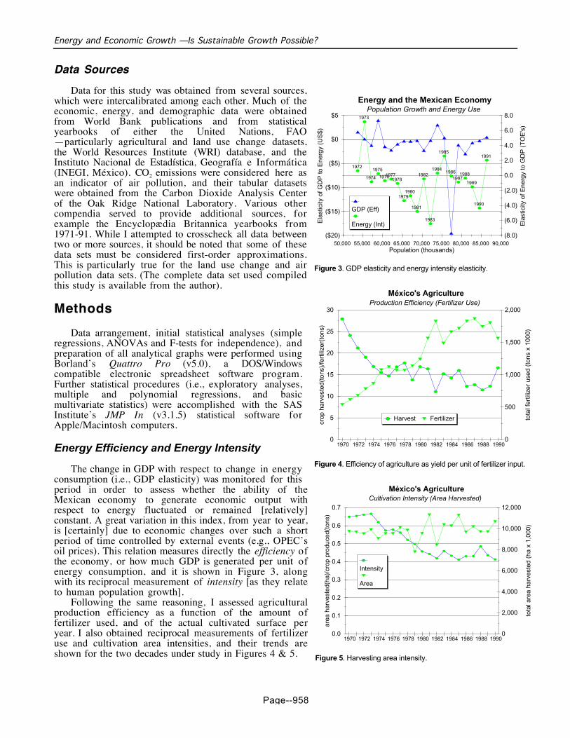
Data SourcesData for this study was obtained from several sources,
which were intercalibrated among each other. Much of theeconomic, energy, and demographic data were obtainedfrom World Bank publications and from statisticalyearbooks of either the United Nations, FAO—particularly agricultural and land use change datasets,the World Resources Institute (WRI) database, and theInstituto Nacional de Estadística, Geografía e Informática(INEGI, México). CO2 emissions were considered here asan indicator of air pollution, and their tabular datasetswere obtained from the Carbon Dioxide Analysis Centerof the Oak Ridge National Laboratory. Various othercompendia served to provide additional sources, forexample the Encyclopædia Britannica yearbooks from1971-91. While I attempted to crosscheck all data betweentwo or more sources, it should be noted that some of thesedata sets must be considered first-order approximations.This is particularly true for the land use change and airpollution data sets. (The complete data set used compiledthis study is available from the author).
MethodsData arrangement, initial statistical analyses (simple
regressions, ANOVAs and F-tests for independence), andpreparation of all analytical graphs were performed usingBorland’s Quattro Pro (v5.0), a DOS/Windowscompatible electronic spreadsheet software program.Further statistical procedures (i.e., exploratory analyses,multiple and polynomial regressions, and basicmultivariate statistics) were accomplished with the SASInstitute’s JMP In (v3.1.5) statistical software forApple/Macintosh computers.
Energy Efficiency and Energy Intensity
The change in GDP with respect to change in energyconsumption (i.e., GDP elasticity) was monitored for thisperiod in order to assess whether the ability of theMexican economy to generate economic output withrespect to energy fluctuated or remained [relatively]constant. A great variation in this index, from year to year,is [certainly] due to economic changes over such a shortperiod of time controlled by external events (e.g., OPEC’soil prices). This relation measures directly the efficiency ofthe economy, or how much GDP is generated per unit ofenergy consumption, and it is shown in Figure 3, alongwith its reciprocal measurement of intensity [as they relateto human population growth].
Following the same reasoning, I assessed agriculturalproduction efficiency as a function of the amount offertilizer used, and of the actual cultivated surface peryear. I also obtained reciprocal measurements of fertilizeruse and cultivation area intensities, and their trends areshown for the two decades under study in Figures 4 & 5.
($20)
($15)
($10)
($5)
$0
$5
Ela
stic
ity o
f GD
P to
Ene
rgy
(US
$)
(8.0)
(6.0)
(4.0)
(2.0)
0.0
2.0
4.0
6.0
8.0
Ela
stic
ity o
f Ene
rgy
to G
DP
(T
OE
's)
50,000 55,000 60,000 65,000 70,000 75,000 80,000 85,000 90,000 Population (thousands)
1972
1973
1974
1975
1976 1977 1978
1979 1980
1981
1982
1983
1984
1985
1986 1987
1988
1989
1990
1991
GDP (Eff)
Energy (Int)
Energy and the Mexican EconomyPopulation Growth and Energy Use
Figure 3. GDP elasticity and energy intensity elasticity.
0
5
10
15
20
25
30
cro
p h
arv
est
ed
(to
ns)
/fe
rtili
zer(
ton
s)
0
500
1,000
1,500
2,000
tota
l fe
rtili
zer
use
d (
ton
s x
10
00
)
1970 1972 1974 1976 1978 1980 1982 1984 1986 1988 1990
Harvest Fertilizer
México's AgricultureProduction Efficiency (Fertilizer Use)
Figure 4. Efficiency of agriculture as yield per unit of fertilizer input.
0.0
0.1
0.2
0.3
0.4
0.5
0.6
0.7
area
har
vest
ed(h
a)/c
rop
prod
uced
(ton
s)
0
2,000
4,000
6,000
8,000
10,000
12,000
tota
l are
a ha
rves
ted
(ha
x 1,
000)
1970 1972 1974 1976 1978 1980 1982 1984 1986 1988 1990
Intensity
Area
México's AgricultureCultivation Intensity (Area Harvested)
Figure 5. Harvesting area intensity.

Proceedings of the 20th Conference of the International Association of Energy Economics, Vol. III
Page--959
Results
Time Series
GDP was extremely highly correlated with 1) population growth, and 2) energy use, supporting my firsthypothesis (Fig 6). The trends of net energy intensity and efficiency (Fig 7), air pollution (Fig 8), land usechange (Fig 9), agricultural yield for cereals, and fertilizer use, summarize the strong positive influence thatboth population growth and energy use exert on the observed economic performance.
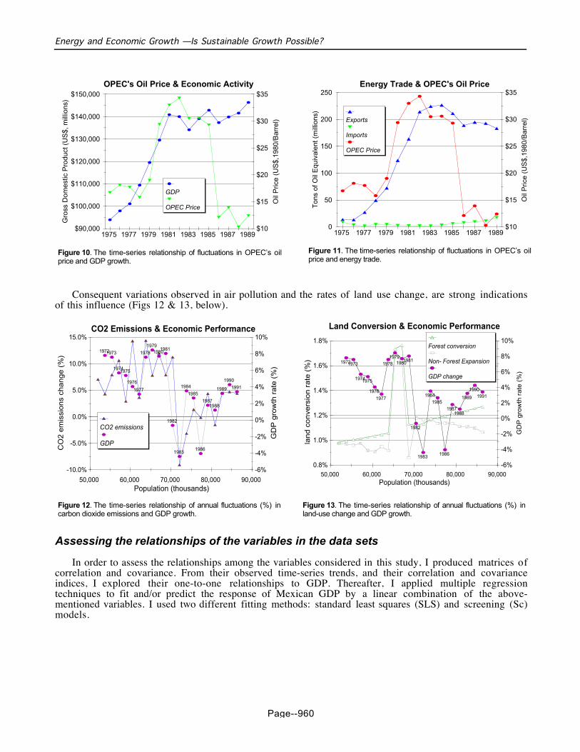
Independently, the rate of change in both GDP and energy production was dramatically influenced byOPEC’s oil price between 1975 and 1989 (Figs 10 & 11, next page).
$0
$40,000
$80,000
$120,000
$160,000
Gro
ss D
om
est
ic P
rod
uct
($
US
, m
illio
ns)
0
50
100
150
200
250
300
350
To
ns
of
Oil
Eq
uiv
alen
t (m
illio
ns)
50,000 60,000 70,000 80,000 90,000 Population (thousands)
1971 1972
1973 1974
1975 1976
1977
1978
1979
1980
1981 1982 1983
1984 1985
1986 1987 1988 1989
1990 1991
GDP
Energy Use
GDP & Energy Use vs. Population
Figure 6. Time-series relationship of GDP growth and energyconsumption, with population.
1.5
1.6
1.7
1.8
1.9
2.0
2.1
To
ns
of
Oil
Eq
uiv
ale
nt/
US
$ (
tho
usa
nd
s)
$480
$500
$520
$540
$560
$580
$600
$620
$640
$660
US
$ (
tho
usa
nd
s)/T
on
s o
f O
il E
qu
iva
len
t
50,000 55,000 60,000 65,000 70,000 75,000 80,000 85,000 90,000 Population (thousands)
1971
1972 1973
1974
1975
1976
1977
1978 1979
1980 1981
1982 1983
1984 1985
1986
1987
1988
1989 1990 1991
Intensity
Efficiency
Efficiency and Intensity of EnergyEconomic Performance and Energy Use
Figure 7. Time-series relationship of economic energy efficiency andenergy intensity, with population.
38,000
40,000
42,000
44,000
46,000
48,000
50,000
52,000
54,000
Cov
erag
e (h
a x
1,00
0)
$60,000
$80,000
$100,000
$120,000
$140,000
$160,000
Gro
ss D
omes
tic P
rodu
ct (
US
$, m
illio
ns)
50,000 60,000 70,000 80,000 90,000 Population (thousands)
1971
1972
1973 1974
1975 1976
1977
1978
1979
1980
1981 1982
1983 1984
1985
1986 1987 1988
1989
1990
1991
"Other" Land Forest Cover GDP
Land Use Change & Economic Activity
Figure 9. The time-series relationship of land-use change and GDPgrowth, with population.
20
30
40
50
60
70
80
90
100
Ton
s of
Car
bon
(m
illio
ns)
100
150
200
250
300
350
Ton
s of
Oil
Equ
ival
ent (
mill
ions
)
50,000 60,000 70,000 80,000 90,000 Population (thousands)
1970 1971
1972 1973
1974 1975 1976
1977
1978
1979
1980
1981
1982 1983 1984
1985 1986 1987
1988
1989
1990 1991
CO2 emissions
Energy use
Energy Consumption & CO2 Release
Figure 8. The time-series relationship of carbon dioxide emissionsand energy consumption, with population.
Energy and Economic Growth —Is Sustainable Growth Possible?
Page--960
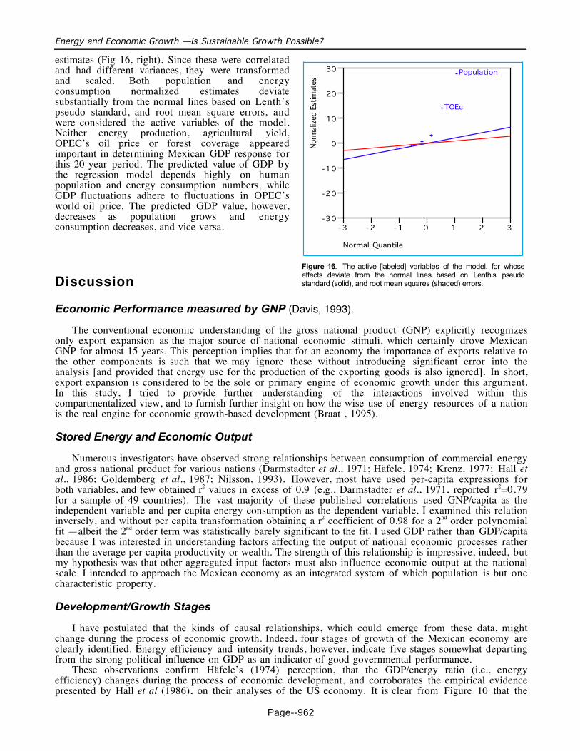
Consequent variations observed in air pollution and the rates of land use change, are strong indicationsof this influence (Figs 12 & 13, below).
Assessing the relationships of the variables in the data sets
In order to assess the relationships among the variables considered in this study, I produced matrices ofcorrelation and covariance. From their observed time-series trends, and their correlation and covarianceindices, I explored their one-to-one relationships to GDP. Thereafter, I applied multiple regressiontechniques to fit and/or predict the response of Mexican GDP by a linear combination of the above-mentioned variables. I used two different fitting methods: standard least squares (SLS) and screening (Sc)models.
$90,000
$100,000
$110,000
$120,000
$130,000
$140,000
$150,000
Gro
ss D
omes
tic P
rodu
ct (
US
$, m
illio
ns)
$10
$15
$20
$25
$30
$35
Oil
Pric
e (U
S$,
1980
/Bar
rel)
1975 1977 1979 1981 1983 1985 1987 1989
GDP
OPEC Price
OPEC's Oil Price & Economic Activity
Figure 10. The time-series relationship of fluctuations in OPEC’s oilprice and GDP growth.
0
50
100
150
200
250
Ton
s of
Oil
Equ
ival
ent (
mill
ions
)
$10
$15
$20
$25
$30
$35
Oil
Pric
e (U
S$,
1980
/Bar
rel)
1975 1977 1979 1981 1983 1985 1987 1989
Exports
Imports
OPEC Price
Energy Trade & OPEC's Oil Price
Figure 11. The time-series relationship of fluctuations in OPEC’s oilprice and energy trade.
0.8%
1.0%
1.2%
1.4%
1.6%
1.8%
lan
d c
on
vers
ion
ra
te (
%)
-6%
-4%
-2%
0%
2%
4%
6%
8%
10%
GD
P g
row
th r
ate
(%
)
50,000 60,000 70,000 80,000 90,000 Population (thousands)
1972 1973
1974 1975
1976
1977
1978 1979
1980 1981
1982
1983
1984 1985
1986
1987 1988
1989
1990 1991
Forest conversion
Non- Forest Expansion
GDP change
Land Conversion & Economic Performance
Figure 13. The time-series relationship of annual fluctuations (%) inland-use change and GDP growth.
-10.0%
-5.0%
0.0%
5.0%
10.0%
15.0%
CO
2 e
mis
sio
ns
cha
ng
e (
%)
-6%
-4%
-2%
0%
2%
4%
6%
8%
10%
GD
P g
row
th r
ate
(%
)
50,000 60,000 70,000 80,000 90,000 Population (thousands)
1972 1973
1974 1975
1976
1977
1978
1979 1980
1981
1982
1983
1984
1985
1986
1987 1988
1989
1990
1991
CO2 emissions
GDP
CO2 Emissions & Economic Performance
Figure 12. The time-series relationship of annual fluctuations (%) incarbon dioxide emissions and GDP growth.

Proceedings of the 20th Conference of the International Association of Energy Economics, Vol. III
Page--961
Table 1
Response: GDPSummary of Fit
RSquare 0.992114RSquare Adj 0.986199Root Mean Square Error 2141.18Mean of Response 127580.3Observations (or Sum Wgts) 15
Parameter Estimates
Term Estimate Std Error t Ratio Prob>|t|Intercept 969088.22 478660.9 2.02 0.0775Population -3.968313 2.137144 -1.86 0.1004TOEc 541.42167 144.9278 3.74 0.0057TOEp -108.2774 38.77059 -2.79 0.0235AgYield -7938.948 9018.705 -0.88 0.4044Oil Price 558.54085 214.6336 2.60 0.0315Forests -13.68437 6.79168 -2.01 0.0787
The SLS is a standard linear fitting procedure which features a summary of fit and parameter estimates(Table 1) The whole-model [regression] hypothesis is shown graphically using a scatter plot of actualresponse values against the predicted ones (Fig 14, above). The whole model F test is significant foranalyzing the response of Mexican GDP to the variables considered. Notwithstanding the evident multipleco linearity problem, all but the agricultural yield regressor contribute to the model fit since their effects aresignificant at the 0.05 level.
Of the six factors considered, there are only a few that stand out in comparison with others. These arehuman population and energy consumption numbers as shown using the screening model3 approach. Theresulting prediction profiler shows the predicted response of GDP for each combination of factor settings. Ijudged the importance of each factor in this way, and found also that statistically there is remarkableinteraction effect between both the human population and energy consumption factors, since the slope ofGDP changes dramatically when they both are modified (Fig 15, below).
One step further into judging the estimates’ effect on the predicted value of the response, such that theycan be compared with each other on fair [statistical] terms, consists of analyzing a normal plot of parameter 3 This approach is designed to analyze experimental data where there are many effects but few observations. Sincethe goal here was to optimize GDP response rather than to show statistical significance, the factor combinations thatoptimized the predicted response were of overriding interest.
GD
P
90000
100000
110000
120000
130000
140000
150000
90000100000 120000 140000GDP Predicted
Figure 14. The whole model [regression] hypothesis.
GDP
146372
93944
127456.2
Desi
rabi
lity 1
0
0.639204
Population
5887
6
8267
770600
TOEc145.
7434
289.
9994233.383
TOEp148.
5838
501.
8319372.805
AgYield1.72
97
2.43
122.12898
Oil Price
10.3
34.321.54
Forests
4300
0
5115
046958
Desirability
0 1
Figure 15. Prediction profiler.
Energy and Economic Growth —Is Sustainable Growth Possible?
Page--962
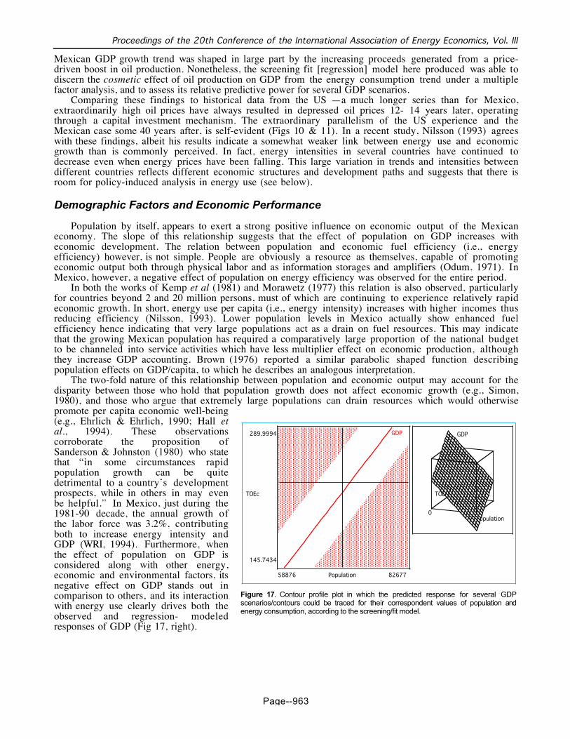
estimates (Fig 16, right). Since these were correlatedand had different variances, they were transformedand scaled. Both population and energyconsumption normalized estimates deviatesubstantially from the normal lines based on Lenth’spseudo standard, and root mean square errors, andwere considered the active variables of the model.Neither energy production, agricultural yield,OPEC’s oil price or forest coverage appearedimportant in determining Mexican GDP response forthis 20-year period. The predicted value of GDP bythe regression model depends highly on humanpopulation and energy consumption numbers, whileGDP fluctuations adhere to fluctuations in OPEC’sworld oil price. The predicted GDP value, however,decreases as population grows and energyconsumption decreases, and vice versa.
Discussion
Economic Performance measured by GNP (Davis, 1993).
The conventional economic understanding of the gross national product (GNP) explicitly recognizesonly export expansion as the major source of national economic stimuli, which certainly drove MexicanGNP for almost 15 years. This perception implies that for an economy the importance of exports relative tothe other components is such that we may ignore these without introducing significant error into theanalysis [and provided that energy use for the production of the exporting goods is also ignored]. In short,export expansion is considered to be the sole or primary engine of economic growth under this argument.In this study, I tried to provide further understanding of the interactions involved within thiscompartmentalized view, and to furnish further insight on how the wise use of energy resources of a nationis the real engine for economic growth-based development (Braat , 1995).
Stored Energy and Economic Output
Numerous investigators have observed strong relationships between consumption of commercial energyand gross national product for various nations (Darmstadter et al., 1971; Häfele, 1974; Krenz, 1977; Hall etal., 1986; Goldemberg et al., 1987; Nilsson, 1993). However, most have used per-capita expressions forboth variables, and few obtained r2 values in excess of 0.9 (e.g., Darmstadter et al., 1971, reported r2=0.79for a sample of 49 countries). The vast majority of these published correlations used GNP/capita as theindependent variable and per capita energy consumption as the dependent variable. I examined this relationinversely, and without per capita transformation obtaining a r2 coefficient of 0.98 for a 2nd order polynomialfit —albeit the 2nd order term was statistically barely significant to the fit. I used GDP rather than GDP/capitabecause I was interested in understanding factors affecting the output of national economic processes ratherthan the average per capita productivity or wealth. The strength of this relationship is impressive, indeed, butmy hypothesis was that other aggregated input factors must also influence economic output at the nationalscale. I intended to approach the Mexican economy as an integrated system of which population is but onecharacteristic property.
Development/Growth Stages
I have postulated that the kinds of causal relationships, which could emerge from these data, mightchange during the process of economic growth. Indeed, four stages of growth of the Mexican economy areclearly identified. Energy efficiency and intensity trends, however, indicate five stages somewhat departingfrom the strong political influence on GDP as an indicator of good governmental performance.
These observations confirm Häfele’s (1974) perception, that the GDP/energy ratio (i.e., energyefficiency) changes during the process of economic development, and corroborates the empirical evidencepresented by Hall et al (1986), on their analyses of the US economy. It is clear from Figure 10 that the
Norm
alize
d Es
timat
es
-30
-20
-10
0
10
20
30 Population
TOEc
- 3 - 2 - 1 0 1 2 3
Normal Quantile
Figure 16. The active [labeled] variables of the model, for whoseeffects deviate from the normal lines based on Lenth’s pseudostandard (solid), and root mean squares (shaded) errors.
Proceedings of the 20th Conference of the International Association of Energy Economics, Vol. III
Page--963
Mexican GDP growth trend was shaped in large part by the increasing proceeds generated from a price-driven boost in oil production. Nonetheless, the screening fit [regression] model here produced was able todiscern the cosmetic effect of oil production on GDP from the energy consumption trend under a multiplefactor analysis, and to assess its relative predictive power for several GDP scenarios.
Comparing these findings to historical data from the US —a much longer series than for Mexico,extraordinarily high oil prices have always resulted in depressed oil prices 12- 14 years later, operatingthrough a capital investment mechanism. The extraordinary parallelism of the US experience and theMexican case some 40 years after, is self-evident (Figs 10 & 11). In a recent study, Nilsson (1993) agreeswith these findings, albeit his results indicate a somewhat weaker link between energy use and economicgrowth than is commonly perceived. In fact, energy intensities in several countries have continued todecrease even when energy prices have been falling. This large variation in trends and intensities betweendifferent countries reflects different economic structures and development paths and suggests that there isroom for policy-induced analysis in energy use (see below).
Demographic Factors and Economic Performance
Population by itself, appears to exert a strong positive influence on economic output of the Mexicaneconomy. The slope of this relationship suggests that the effect of population on GDP increases witheconomic development. The relation between population and economic fuel efficiency (i.e., energyefficiency) however, is not simple. People are obviously a resource as themselves, capable of promotingeconomic output both through physical labor and as information storages and amplifiers (Odum, 1971). InMexico, however, a negative effect of population on energy efficiency was observed for the entire period.
In both the works of Kemp et al (1981) and Morawetz (1977) this relation is also observed, particularlyfor countries beyond 2 and 20 million persons, must of which are continuing to experience relatively rapideconomic growth. In short, energy use per capita (i.e., energy intensity) increases with higher incomes thusreducing efficiency (Nilsson, 1993). Lower population levels in Mexico actually show enhanced fuelefficiency hence indicating that very large populations act as a drain on fuel resources. This may indicatethat the growing Mexican population has required a comparatively large proportion of the national budgetto be channeled into service activities which have less multiplier effect on economic production, althoughthey increase GDP accounting. Brown (1976) reported a similar parabolic shaped function describingpopulation effects on GDP/capita, to which he describes an analogous interpretation.
The two-fold nature of this relationship between population and economic output may account for thedisparity between those who hold that population growth does not affect economic growth (e.g., Simon,1980), and those who argue that extremely large populations can drain resources which would otherwisepromote per capita economic well-being(e.g., Ehrlich & Ehrlich, 1990; Hall etal., 1994). These observationscorroborate the proposition ofSanderson & Johnston (1980) who statethat “in some circumstances rapidpopulation growth can be quitedetrimental to a country’s developmentprospects, while in others in may evenbe helpful.” In Mexico, just during the1981-90 decade, the annual growth ofthe labor force was 3.2%, contributingboth to increase energy intensity andGDP (WRI, 1994). Furthermore, whenthe effect of population on GDP isconsidered along with other energy,economic and environmental factors, itsnegative effect on GDP stands out incomparison to others, and its interactionwith energy use clearly drives both theobserved and regression- modeledresponses of GDP (Fig 17, right).
289.9994
TOEc
145.7434
GDP
58876 Population 82677
0Population
TOEc
GDP
Figure 17. Contour profile plot in which the predicted response for several GDPscenarios/contours could be traced for their correspondent values of population andenergy consumption, according to the screening/fit model.
Energy and Economic Growth —Is Sustainable Growth Possible?
Page--964
Renewable Energy Resources and Economic Production
The area dimensions of a nation appear to contribute to total GDP output (Kemp et al., 1981).Although not analyzed explicitly here, it could be expected that Mexico, with an area of 191 millionhectares [52% of those considered domesticated], could generate considerable economic output per unit ofarea in agricultural, forestry, or fisheries resources. This might be explained by the fact that greater areagenerally captures greater solar energy (which is important for agrarian-based economies), while people aremost important (in a production sense) as reservoirs and manipulators of information, which becomesincreasingly significant with the intricacies of industrializing [-ed] countries.
The latter seems to be the Mexican case since only as little as 8% of GDP originated from agriculture,30.7% from industry and 61.3% from services during 1991 (WRI, 1994). The implication here is that theserenewable resources (or directly derived-solar energies), do not contribute significantly to Mexico’seconomic output.
In fact agricultural production in Mexico appearsdriven by GDP performance, which in turn drives thefertilizer production/purchase, and use necessary tosustain agricultural yields at “commercial” levels.
Deforestation and land-conversion for cattleranching, and urban and industrial settlements seemalso to be driven by GDP in the same way.
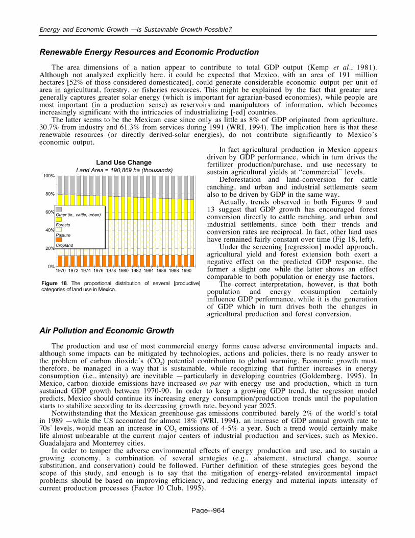
Actually, trends observed in both Figures 9 and13 suggest that GDP growth has encouraged forestconversion directly to cattle ranching, and urban andindustrial settlements, since both their trends andconversion rates are reciprocal. In fact, other land useshave remained fairly constant over time (Fig 18, left).
Under the screening [regression] model approach,agricultural yield and forest extension both exert anegative effect on the predicted GDP response, theformer a slight one while the latter shows an effectcomparable to both population or energy use factors.
The correct interpretation, however, is that bothpopulation and energy consumption certainlyinfluence GDP performance, while it is the generationof GDP which in turn drives both the changes inagricultural production and forest conversion.
Air Pollution and Economic Growth
The production and use of most commercial energy forms cause adverse environmental impacts and,although some impacts can be mitigated by technologies, actions and policies, there is no ready answer tothe problem of carbon dioxide’s (CO2) potential contribution to global warming. Economic growth must,therefore, be managed in a way that is sustainable, while recognizing that further increases in energyconsumption (i.e., intensity) are inevitable —particularly in developing countries (Goldemberg, 1995). InMexico, carbon dioxide emissions have increased on par with energy use and production, which in turnsustained GDP growth between 1970-90. In order to keep a growing GDP trend, the regression modelpredicts, Mexico should continue its increasing energy consumption/production trends until the populationstarts to stabilize according to its decreasing growth rate, beyond year 2025.
Notwithstanding that the Mexican greenhouse gas emissions contributed barely 2% of the world’s totalin 1989 —while the US accounted for almost 18% (WRI, 1994), an increase of GDP annual growth rate to70s’ levels, would mean an increase in CO2 emissions of 4-5% a year. Such a trend would certainly makelife almost unbearable at the current major centers of industrial production and services, such as Mexico,Guadalajara and Monterrey cities.
In order to temper the adverse environmental effects of energy production and use, and to sustain agrowing economy, a combination of several strategies (e.g., abatement, structural change, sourcesubstitution, and conservation) could be followed. Further definition of these strategies goes beyond thescope of this study, and enough is to say that the mitigation of energy-related environmental impactproblems should be based on improving efficiency, and reducing energy and material inputs intensity ofcurrent production processes (Factor 10 Club, 1995).
0%
20%
40%
60%
80%
100%
1970 1972 1974 1976 1978 1980 1982 1984 1986 1988 1990
Other (ie., cattle, urban)
Forests
Pasture
Cropland
Land Use ChangeLand Area = 190,869 ha (thousands)
Figure 18. The proportional distribution of several [productive]categories of land use in Mexico.

Proceedings of the 20th Conference of the International Association of Energy Economics, Vol. III
Page--965
Filling the GNP Gap under NAFTA
Assuming that the observed correlations and predicted responses of GDP to demographic and energyfactors are indicative of causal relationships, we may ask how can Mexico exploit available renewableresources in a sustainable basis to raise its GNP/capita, in relation to its new partners in free-trade. Since lessdeveloped nations tend to have the best GDP/energy ratios (i.e., their energy intensities are low4), it isunlikely that economic output could be improved by achieving even higher fuel efficiencies. In fact,Goldemberg (1995) is emphatic in noting that a transitional period of particularly low economic efficiencycan be anticipated before full economic development is achieved, which is exactly what Mexico has gonethrough for the last 25 years!
In contrast to the oil-based economy of Mexico, many other developing nations have been utilizingrenewable energy resources directly through agriculture and fisheries (Scrimshaw & Taylor, 1980), draftanimals (Ward et al., 1980), hydroelectric power (Strout, 1977; Hammond, 1978), and biomass fuels(Ramachandran & Gururaja, 1977). Hence, one alternative to bridge the gap between Mexico and itscurrent NAFTA partners could be the judicious use of its fossil fuel reserves, along with the management ofenergy-related environmental impact problems, as mentioned above. The best alternative to expandMexican GDP, however, would be the direct [sustainable] exploitation of solar-based resources. Whetheremphasis should be placed on agriculture, fisheries, hydroelectric or biomass ‘fuels’, will depend on theparticular endorsement of the renewable energies available, along with the social, political, and economicdirections adopted by its government. One option may very well conflict with another, for example theconversion of truck-crop fields into sugar cane plantations for production of alcohol seems inadequate inthe face of an undernourished population. The macroscopic perspective that I have used, while notappropriate for addressing social/economic issues in detail, provides a salient view of the broad horizons foreconomic development.
From the proportion of the total renewable resources that Mexico could use directly some importantpercentage of insolation can be channeled into agriculture, fisheries and forestry, while just about half ofthe hydrostatic potential can be tapped into electric power generation under ideal conditions of topographyand precipitation. The question is, how much increase in GDP can be obtained by exploiting these availablerenewables? Further analysis of these interactions is necessary to properly address this question.
ConclusionI have undertaken a macroscopic perspective of the Mexican economy as it entered into the
industrialized world, considering its structure in a very aggregated form. I tried to follow Bratt’s (1995)approach into linking the systems ecology approach to issues of development in Mexico. In any case, Imaintain that this scale of analysis facilitates one’s competence to see gross interrelationships. Since it isvirtually impossible to conduct experiments at the level of a national economy—at least not withoutdynamic modeling, analyses of this kind of data are necessarily inductive in approach. I was limited to theuse of statistical correlations and simple multi-factor analyses, which per se are inappropriate for addressingissues of causality. I have, nonetheless used these statistics to draw inferences on cause-effect couplets inreference to the hypothesized structure of the national system conceptualized at the outset. I cannot,however, rule out the possibility that the relationships observed and described here are simplymanifestations of co variances with some third factors, which I did not consider [at all].
Acknowledgements
This paper is part of an ongoing doctoral dissertation research funded in part by the Consejo Nacional de Ciencia yTecnología (CONACyT, México), and the Fulbright Commission at the Institute for International Education (FC-IIE,USA) endorses it. All work was done under the supervision of Charles A. S. Hall, Professor of Systems Ecology andEnergy Analysis at the State University of New York College of Environmental Science & Forestry (SUNY-ESF,USA). Both the Tata Energy Research Institute (TERI, India), and the Randolph G. Pack Environmental Institute atSUNY-ESF, provided financial support to present this paper at the 20th Conference of the International Association ofEnergy Economics (New Delhi, India: January 22-24, 1997).
4 Excluding non-commercial energy. Otherwise, their energy intensities might be similar to those of high incomecountries (Nilsson, 1993).

Energy and Economic Growth —Is Sustainable Growth Possible?
Page--966
References
Ausubel, JH, 1996. Can technology spare the Earth? American Scientist 84: 166- 178.Braat, LC, 1995. Systems ecology and sustainable development, In : Hall, CAS (Ed), Maximum Power: The Ideas and
Applications of HT Odum, 164- 174 pp. The University Press of Colorado, Niwott.Brown, H, 1976. Energy in our future. Annual Review of Energy 1: 1- 36.Cottrell, F, 1955. Energy and Society. McGraw-Hill, New York (Reprinted by Greenwood Press, Westport).Daly, HE & KN Townsend, 1993. Valuing the Earth: Economics, Ecology and Ethics. The MIT Press, Cambridge.Darmstadter, T, PD Teitelbaum & TG Polach, 1971. Energy in the World Economy: A Statistical Survey of Trends in
Output, Trade and Consumption since 1925. The Johns Hopkins University Press, Baltimore.Davis, HC, 1993. Regional Economic Impact Analysis and Project Evaluation. UBC, Vancouver.Ehrlich, P & A Ehrlich, 1990. The Population Explosion. Simon and Schuster, New York.Factor 10 Club/Club of Rome, 1995. Carnoules Declaration 1995. Wuppertal Institute, Germany.Frosch, RA & NE Gallopoulos, 1989. Strategies for manufaturing. Scientific American 261: 144- 153.Goldemberg, J, 1995. Energy needs in developing countries and sustainability. Science 269: 1058- 1059.Goldemberg, J, TB Johansson, AKN Reddy & RH Williams, 1987. Energy for a Sustainable World. World Resources
Institute, Washington.Häfele, W, 1974. Energy choices that Europe faces: A European view of energy. Science 184: 360.Hall, CAS, 1992. Economic development or developing economics: what are our priorities, In : Wali, MK & JS Singh
(Eds), Environmental Rehabilitation, Vol 1- Policy Issues, 101- 126 pp. Elsevier, Amsterdam.Hall, CAS, C Cleveland & R Kaufmann, 1986. Energy and Resource Quality: The Ecology of the Economic Process.
Wiley Interscience, New York (Reprinted by The University of Colorado Press, Niwot).Hall, CAS, G Pontius, J-Y Ko & L Coleman, 1994. The environmental impact of having a baby in the United States.
Population and Environment 15: 505- 523.Hammond, AL, 1978. Energy: Elements of a Latin American strategy. Science 200: 753- 754.Kemp, WM, WR Boynton & K Limburg, 1981. The influence of natural resources and demographic factors on the
economic production of nations, In : Mitsch, WJ, RW Bosserman & JM Klopatec (Eds), Energy and EcologicalModelling, 827- 839 pp. Elsevier Scientific Publishing Co., Amsterdam.
Krenz, JH, 1977. Energy and the economy: An interrelated perspective. Energy 2: 115- 130.Leontief, W, 1974. Structure of the world economy: Outline of a simple input-output formulation. American
Economics Review 64: 823- 834.MacNeill, J, 1989. Strategies for sustainable economic development. Scientific American 261: 154-165.Morawetz, D, 1977. Twenty-five years of economic development: 1950- 1975. The World Bank, Washington (A 126
pages report).Nilsson, LJ, 1993. Energy intensity trends in 31 industrial and developing countries 1950-1988. Energy 18: 309- 322.Odum. HT, 1971, Environment, Power and Society. John Wiley & Sons, Inc. New York.Odum, HT, 1996. Environmental Accounting: Emergy and Decision Making. John Wiley, New York.Pimentel, D, M Herdendorf, S Eisenfeld, L Olander, M Carroquino, C Corson, J McDade, Y Chung, W Cannon, J
Roberts, L Bluman & J Gregg, 1995. Achieving a secure energy future: Environmental and economic issues.Ecological Economics 9: 201- 219.
Ramachandran, A & J Gururaja, 1977. Perspectives on energy in India. Annual Review of Energy 2: 365- 386.Sanderson, W & BF Johnston, 1980. Bad news: Is it true? Science 210: 1302- 1303.Scrimshaw, NS & L Taylor, 1980. Food. Scientific American 243: 78- 88.Simon, JL, 1980. Resources, population and environment: An oversupply of bad news. Science 208: 1431- 1437.Strout, AM, 1977. Energy and economic growth in Central America. Annual Review of Energy 2: 291- 305.Vitousek, PM, P Ehrlich, A Ehrlich & P Matson, 1986. Human appropriation of the products of photosynthesis.
Bioscience 36: 368- 373.Ward, GM, TM Southerland & JM Southerland, 1980. Animals as an energy resource in Third World agriculture.
Science 208: 570- 574.World Resources Institute,1994. World Resources 1994- 95: A Guide to the Global Environment —People and the
Environment. Oxford University Press, New York. (In collaboration with the United Nations’ Programmes ofEnvironment [UNEP] and Development [UNDP]).


