
ENHANCEMENTS OF METHANE, BENZENE, AND N-PENTANE BY OIL AND GAS FIELDS
OBSERVED FROM THE DC-3 AIRCRAFT CAMPAIGN: A CASE STUDY
by
CAROLYN MICHELLE FARRIS
B.S., University of Portland, 2011
A thesis submitted to the
Faculty of the Graduate School of the
University of Colorado in partial fulfillment
of the requirement for the degree of
Master’s of Science
Department of Atmospheric and Oceanic Science
2013

This thesis entitled:
Enhancements of methane, benzene, and n-pentane by oil and gas fields observed from the
DC-3 aircraft campaign: A case study
written by Carolyn Michelle Farris
has been approved for the Department of Atmospheric and Oceanic Science
Dr. Katja Friedrich
Dr. Julie Lundquist
Date
The final copy of this thesis has been examined by the signatories, and we
Find that both the content and the form meet acceptable presentation standards
Of scholarly work in the above mentioned discipline.

iii
Farris, Carolyn Michelle (M.S., Atmospheric and Oceanic Science)
Enhancements of methane, benzene, and n-pentane by oil and gas fields observed from the
DC-3 aircraft campaign: A case study
Thesis directed by graduate faculty appointed Teresa Campos
Abstract
Observations in the boundary layer from the 1 June flight in Colorado of the 2012 Deep
Convective Clouds and Chemistry campaign shows enhancements of n-pentane, methane, and
benzene near oil and gas wells that are not correlated with enhancements in carbon monoxide. To
further investigate the source of methane emissions, an i-pentane:n-pentane ratio is compared to
surface measurements from the Denver-Julesberg Basin and found to be similar. Measurements
of n-pentane, methane, benzene and CO are also shown with proximity to Denver to compare an
urban signature with an oil and gas well emissions signature. Elevated n-pentane, methane, and
benzene mixing ratios without enhancements in CO from the 1 June flight are considered to be
strongly influenced by emissions from oil and natural gas fields located near the sampling
locations.

iv
CONTENTS
CHAPTER
1. INTRODUCTION 1
1.1 Motivation 1
1.2 Background 4
2. INSTRUMENTS AND METHODS 8
2.1 Deep Convective Clouds and Chemistry (DC-3) Experiment 8
2.2 Instruments 9
2.2.1 Picarro G1301f Carbon Dioxide and Methane Analyzer 10
2.2.2 Aero-laser AL5002 VUV Resonance Fluorescence CO
Monitor
11
2.2.3 HIAPER-TOGA (Trace Organic Gas Analyzer) 12
2.2.4 Ozone Chemiluminescence Instrument 12
3. RESULTS 13
3.1 DC-3 GV spatial distribution of i-C5/n-C5, methane, n-pentane,
benzene, CO, and O3 boundary layer data
13
3.1.1 Determining the boundary layer height for each GV flight and
discussion of tracer gases
14
3.1.2 Cattle and landfills as other sources of methane 28
3.1.3 Tracer and well proximity correlation plots for GV
measurements within the boundary layer
30
3.1.4 Testing for correlation between proximity to wells and tracer 39

v
data
3.2 1 June 2012 (GV-RF8), Colorado low altitude leg case study 44
3.2.1 Tracer and nearby well correlation plots for research flight 8
case study
50
3.2.2 Testing for correlation for research flight 8 case study 57
4. CONCLUSION 60
WORKS CITED 64
APPENDIX
A. Potential temperature soundings from GV flights 70
B. NEXRAD plots for flight legs with convection 76
C. HYSPLIT plots for flight legs within the boundary layer 78

vi
TABLES
Table
1. Flight times, location, and wind data for flights with sampling time within the boundary
layer. Wind measurements are for times indicated by time of sampling in the second
column. 18
2. Number of nearby wells for GV boundary layer samples 33
3. Student’s t-test results for correlation between tracers and proximity to active oil and gas
wells. Individual flight test results for legs that flew near more than one active well 42
4. Hypothesis test results for case study. Tracers are tested for correlation with proximity to
wells and to Denver 58

vii
FIGURES
Figure
1. Shale basins in the US 2
2. Gulfstream-V sounding profile of potential temperature taken from 21:09 to 21:34 UTC
on 26 May 2012 15
3. i-Pentane:n-Pentane and flight track spatial distribution 19
4. Spatial distributions of GV flight tracks, methane, n-pentane, benzene, CO, and O3 23
5. Map of methane emissions of landfills using 2002 data 28
6. Map of cattle inventory from 2007 29
7. Example of number of "nearby" wells calculation for a flight with highly variable wind
direction (2σ > 90°) 31
8. Example of number of "nearby" wells calculation for a flight with less variable wind
direction (2σ < 90°) 32
9. Iso-Pentane vs. n-Pentane for GV flights within the boundary layer 34
10. CO vs. methane measurements for GV flights within the boundary layer 36
11. Methane vs. benzene and CO vs. benzene for GV flights within the boundary layer 37
12. Methane vs. n-Pentane and CO vs. n-Pentane for GV flights within the boundary layer 38
13. GV RF8 leg 1 sounding 45
14. Denver station sounding 2 June, 2012 at 00:00 UTC 46
15. GV forward camera showing the cloud base, picture taken during research flight 8 on
June 1 at 22:36 UTC [51] 46
16. Flight track for 1 June 2012 (GV research flight 8). 47

viii
17. HYSPLIT back trajectories using GDAS archive data for GV research flight 8. Ensemble
plots are made for the start, middle, and end of the low altitude leg used in the 1 June
case study. 48
18. HYSPLIT back trajectories using GDAS archive data for GV research flight 8. Ensemble
plots are made for the start, middle, and end of the low altitude leg used in the 1 June
case study with altitudes at 1500 m. 49
19. i-Pentane:n-Pentane ratios for research flight 8 in Colorado 51
20. CO vs. methane, CO vs. benzene, and methane vs. benzene for research flight 8 in
Colorado 53
21. CO vs. n-Pentane and methane vs. n-Pentane for research flight 8 in Colorado 55

1
Enhancements of methane, benzene, and n-pentane by oil and gas fields observed from the
DC-3 aircraft campaign: A case study
1. Introduction
1.1 Motivation
North America has the largest natural gas market, making up 29% of the global demand [1].
In the U.S., about a quarter of the energy supply is provided by gas, used primarily for residential
heating and cooking, commercial heating and cooling, electricity generation, and for numerous
industrial applications [1]. Since 2009, the amount of gas reserves in the U.S. rose by 39%
because hydraulic fracturing and new horizontal drilling technologies allow the acquisition of
gas stored in shale formations [1]. Within the U.S., 37% of the natural gas industry is located in
Texas, Oklahoma, and Kansas while about 25% is located in the Gulf of Mexico [2]. Locations
of basins in the U.S. are shown in Figure 1.

2
Figure 1. Shale basins in the US. (Courtesy Energy Information Administration,
http://www.eia.gov/oil_gas/rpd/shale_gas.jpg, updated May 9, 2011). The Denver-Julesberg
Basin, Anadarko Basin, and Fort Worth Basin are indicated by white boxes.
Natural gas is considered by some to be a viable alternative energy source to coal for
significantly reducing CO2 emissions as carbon emissions from natural gas power plants are
about half that of coal plants per unit of electricity produced [3]. It is also regarded as the
cleanest of all fossil fuels, emitting carbon dioxide, water vapor, and small amounts of nitrogen
oxides, sulfur dioxide, carbon monoxide, and reactive hydrocarbons [1]. Other benefits include a
reduction in smog and acid rain because natural gas emits low levels of nitrogen oxides and
sulfur dioxide, and virtually no particulate matter [1]. Methane is a greenhouse gas and a main
constituent of natural gas (about 60-90% CH4 by molecule) and studies by the Environmental

3
Protection Agency (EPA) and the Gas Research Institute (GRI) find that reduction in emissions
from using natural gas outweighs the added methane emissions [4] [1].
Despite these benefits, research from ground based measurements in Colorado, and Texas
and Oklahoma report that methane emissions in the U.S. from natural oil and gas (ONG) wells
may be greater than EPA estimate of 6 ± 2 Tg per year [5] [2]. Enhancements of benzene and
light alkanes (C2 – C5) have also been detected in air masses near natural oil and gas fields [5]
[4]. High wintertime ozone levels in Wyoming and Utah are also attributed to emissions of
VOCs and NOX from natural oil and gas fields [4].
The following study presents data from the Deep Convective Clouds and Chemistry
Project (DC-3) to compare the concentrations of ONG and anthropogenic tracers to a
measurement’s proximity to active wells. Samples near oil and gas wells are inspected for the
enhancement of known oil and gas field emissions: methane, n-pentane and benzene, without an
enhancement in the combustive tracer, CO. The hypotheses that will be tested here are:
1. The concentration of methane in the boundary layer increases in the vicinity of oil and
gas wells.
2. The concentration of n-pentane in the boundary layer increases in the vicinity of oil and
gas wells.
3. The concentration of benzene in the boundary layer increases in the vicinity of oil and
gas wells.
4. The boundary layer concentrations of urban tracers, ozone and CO, do not increase in the
vicinity of oil and gas wells.

4
The data set used is from a flight campaign conducted in Colorado, Oklahoma, and
Alabama with several hours of data collected within the boundary layer and near oil and gas
wells. Strengths of the data set include spatial coverage over Oklahoma and northeastern
Colorado near the Anadarko, Fort Worth, and Denver Basins in the boundary layer. Most
research in oil and gas field emissions are conducted at the surface. However, because the flight
campaign’s intention was to study the chemistry of convective storms rather than focus source
apportionment, the data collected was not always near high concentrations of active wells, and
the atmospheric tracers may have been diluted when measured near convective systems. In
addition, the plane, a Gulfstream V, that held the instruments measuring methane, CO, and other
atmospheric tracers analyzed in this study flew primarily in the outflow of convective storms in
the free troposphere. In nine of twenty-two flights during the campaign, the GV flew into the
boundary layer, with many of the measurement samples occurring near active oil and gas wells.
1.2 Background
Methane has a globally averaged lifetime of about 9 years in the troposphere [6] and is
the second most important long-lived greenhouse gas (GHG) behind CO2 in both radiative
forcing and in abundance, with an average concentration of 1,774.62 ± 1.22 ppb [7].
Concentrations of methane have increased since industrialization beginning at about 1750, giving
an estimate of anthropogenic emissions of 340 ± 50 Tg CH4 yr-1
[7]. Since the 1980s, however,
methane growth rates slowed to almost zero from 1999 to 2005 [7]. Some theories for the
slowing rate are (1) a reduction in the photochemical production of the methane sink, OH, after
the Mount Pinatubo eruption in 1991, (2) slowing methanogenesis in wetlands during Northern
Hemisphere cooling after the Mount Pinatubo eruption, and (3) the economic collapse of the

5
Soviet Union leading to its dissolution in 1991 [8]. Although there are some theories, there is no
consensus on the reason for the decline [9]. Despite its importance in climate forcing and a
global warming potential of 25 for 100 years [5], methane sink and source strengths are still
poorly constrained [10]. Lelieveld, et al. [11] estimates 600 ± 80 Tg of methane is added and
removed from the atmosphere per year. Of that estimate, anthropogenic sources include energy
(120 ± 40 Tg yr-1
), landfills (145 ± 30 Tg yr-1
), domestic ruminants (80 ± 20 Tg yr-1
), rice
agriculture (80 ± 50 Tg yr-1
), and biomass burning (40 ± 30 Tg yr-1
) [11]. Natural sources include
wetlands (145 ± 30 Tg yr-1
), termites (20 ± 20 Tg yr-1
), oceans (10 ± 5 Tg yr-1
), and hydrates (10
± 5 Tg yr-1
) [9] [11]. Atmospheric methane loss rates are influenced primarily (about 90%) by
oxidation with hydroxyl radicals (OH), while minor sinks include photolysis in the stratosphere
(7-11%), and bacterial consumption in soils (1-10%) [11].
Studies in the Denver-Julesberg Fossil Fuel Basin (DJB) in Northeastern Colorado and in
the Anadarko Basin of Texas and Oklahoma reveal oil and natural gas field emissions of
methane that may be currently underestimated by industry inventories [5] [2]. During a 2002
study in the southwestern United States, methane emissions from oil and gas fields in Kansas,
Texas, and Oklahoma are estimated to be 4-6 Tg per year, indicating that the previous
approximation by the EPA of total US oil and gas emissions of 6 ± 2 Tg is underestimated [2].
Similarly, measurements in the DJB imply methane emissions may be twice as large as expected
from natural gas systems in Colorado [5]. During gas production, methane can be released during
flow-back of hydraulic fracturing fluids, drill-out of plugs, equipment leaks, processing,
transport, storage, and distribution [10]. Howarth et al. [10] reports that a well loses 3.6% - 7.9%
of methane from shale gas production through venting and fugitive emissions over the course of
the well’s lifetime. Comparing shale gas to coal, the GHG footprint for shale gas is at least 20%

6
greater than that of coal on a twenty year time horizon, but the energy sources’ footprints are
about equal for 100 years due to the shorter residence time of methane to CO2 [10]. Although a
100 year time horizon is more commonly used, the 20 year time scale is crucial for monitoring
methane to avoid accelerating climatic positive feedback loops [12].
Benzene is a known carcinogen with significant concentrations in ambient air due
primarily to vehicle emissions [13]. The atmospheric lifetime for benzene is 57 hours and is
removed from the atmosphere largely through reactions with OH [14] as benzene reacts too
slowly with O3 and NO3 radicals to make them important removal mechanisms in the atmosphere
(rate constant for O3 reaction <1 x 10-20
cm3 molec
-1 s
-1 and 10
-16 to 10
-17 cm
3 molec
-1 s
-1 for
NO3 reaction at room temperature) [15]. Because removal of benzene is dominated by reactions
with OH, concentrations of benzene are lowest in the summer months when more solar radiation
and higher temperatures allow for greater production of OH, as well as more mixing with
background air that is lower in benzene concentrations [14]. Other sources of benzene include
solvent evaporation, industrial process emissions, service stations for motor vehicles, and oil and
natural gas fields [13] [14] [5].
In addition to emitting methane and light alkanes, oil and natural gas fields can also emit
benzene at various stages of production: during glycol regeneration at glycol dehydrators, while
venting and flaring, through engine exhaust, and at condensate tanks, compressors, processing
plants [5]. Hydraulic fracturing fluid, used to further fragment shale formations and carry
proppants to hold open fractures, can also contain varying amounts of benzene depending on the
site [16]. Diesel fuel is used in the slurry of some gelled fracturing fluids that increase the
viscosity to better transport proppants to fractures, making up 30%-100% of the thickener [16].

7
When diesel fuel is used, the EPA finds that benzene exceeds the maximum contaminant level at
the point of injection in the well when benzene makes up 0.000026 to 0.001% by weight in
diesel fuel [16]. Though few service companies currently use diesel fuel, a study by Petron et al.
[5] in the DJB estimates top-down benzene emissions of 639-1145 tonnes/yr from oil and gas
production compared to 3.9 tonnes/yr estimated by reporting facilities to the EPA.
Due to their short lifetimes ranging from a couple months to a few days, concentrations
of light alkanes are highly variable due to meteorology and are strongly influenced by nearby
sources. Sources of n-alkanes include fossil fuel combustion, biomass burning, suspension of
pollen, micro-organisms, and bacteria [17]. Cattle feedlots also emit lighter n-alkanes, but do not
substantially affect levels of n-butane or n-pentane [5]. Iso-alkanes are emitted from evaporation
of liquefied petroleum gas and automobile fuel, and biomass burning [17]. Natural gas also emits
n- and iso-alkanes during production, storage, and transport, and enhancements of C2-C5 alkanes
were found during ground measurements in the southwestern US as well as northeastern
Colorado near oil and gas fields [18] [2] [5]. Photochemistry and reactions with OH are the
dominate sinks for both n- and iso-alkanes [17] [18].
Carbon monoxide is also analyzed in this study as a tracer for air masses influenced by
combustion. Major sources of carbon monoxide are fossil fuel combustion, biomass burning, and
the oxidation of hydrocarbons [19]. Carbon monoxide’s primary sink is oxidation by OH and its
lifetime can range between a few weeks to several months in the troposphere depending on the
amount of solar radiation, with its shortest lifetime occurring in the summer months [19]. CO is
not a greenhouse gas itself, but it does affect the lifetime of methane as both are oxidized by OH.
8
As CO increases, more OH is used in the oxidation of carbon monoxide, lengthening the lifetime
of methane [20].
Ozone is measured onboard the GV and included in the following analysis. Although
ozone absorbs biologically active UV-B radiation in the stratosphere, tropospheric ozone near
the surface is damaging to human health, specifically affecting the respiratory system, and can
reduce crop yield [21] [22]. With a global radiative forcing of 0.35 ± 0.15 W/m2, ozone is a
significant greenhouse gas behind the longer-lived greenhouse gases like CO2 and CH4 [7]. In-
situ photochemical reactions of methane, VOCs, and NOX produce the majority of tropospheric
ozone with production rates dependent on the concentration of NOX, and a minor amount (about
10%) is from stratospheric intrusions [23]. A small amount of ozone can also be produced
naturally from the photolysis of O2, resulting in ozone mixing ratios of 10-40 ppb in pristine
unpolluted air [22]. Ozone is removed from the troposphere primarily through dry deposition
[23].
2. Instruments and Methods
2.1 Deep Convective Clouds and Chemistry (DC-3) Experiment [24]
In May and June of 2012, the National Oceanic and Atmospheric Association (NOAA),
the National Aeronautics and Space Administration (NASA), and the National Science
Foundation (NSF) conducted a field campaign to characterize inflow and outflow of midlatitude
convective storms in the regions of northeastern Colorado, west Texas to central Oklahoma, and
northern Alabama. The Deep Convective Clouds and Chemistry Project (DC3) campaign used

9
three aircraft: the NASA DC-8, the NSF/NCAR Gulfstream V (GV) and the DLR (Deutsches
Zentrum für Luft- und Raumfahrt) Falcon operating out of the Salina, Kansa airport. The GV
primarily flew in the upper troposphere at about 10 to 12 km to measure convective outflow,
complementing DC-8 flights at lower altitudes to measure inflow. The campaign targeted three
types of continental convective storms: air mass, multicell and supercell thunderstorms, and
mesoscale convective systems.
The GV is a High-Performance Instrumented Airborne Platform for Environmental
Research (HIAPER) aircraft with a maximum altitude of about 15 km. Most GV flights lasted
five to eight hours, usually taking off and landing in Salina, Kansas. Intercomparison legs with
the DC-8 occurred in some flights to harmonize measurements of species sampled on both
aircraft to test instrument precision and accuracy. The GV typically sampled outflow, but for the
case flight investigated in this study, the GV flew between 2.4 and 2.7 km for 80 minutes. The
GV’s instrument payload had over ten instruments, including a Picarro G1301f measuring CO2
and methane, an Aero-Laser AL5002 measuring CO, and the Trace Organic Gas Analyzer which
measured i-pentane, n- pentane, and benzene, and an ozone chemiluminescence instrument.
These chemical species are considered in this study.
2.2 Instruments
The GV flew at a ground speed of about 200 m/s for most flights. The Picarro, Aero-
Laser and ozone chemiluminescence instrument made measurements once per second,
corresponding to one measurement every 200 m relative to the ground. TOGA sampled once
every two minutes, with a spatial resolution of 24 km relative to the ground.

10
2.2.1 Picarro G1301f Carbon Dioxide and Methane Analyzer [25] [26]
A Picarro G1301f onboard the GV measured CO2 and methane using Wavelength-
Scanned Cavity Ring Down Spectroscopy (WS-CRDS) [25]. In WS-CRDS, a cavity is first filled
with analyte gas from ambient air during flight. A tunable diode laser aims into the cavity, tunes
across several different wavelengths, and reflects multiple times between three mirrors within the
cavity, increasing the path length up to 20 km which enhances sensitivity to trace gas absorption
of infrared light. A photodetector behind one of the mirrors detects the amount of light that leaks
through the mirror, and this signal is proportional to the intensity of light inside the cavity. Once
an intensity threshold is reached, the laser shuts off and the signal decays due to imperfections in
the mirrors and gas species that absorb the light. Concentrations of CO2 and methane are
proportional to the difference in decay times at wavelengths where gases are strongly absorbing
and wavelengths where they do not absorb. A long effective path length, high precision
wavelength monitor, and temperature and pressure controls enable the analyzer to maintain high
accuracy, precision, and linearity over a range of environmental conditions and long periods of
time. The G1301f has a precision of 250 ppbv and 3 ppbv for CO2 and methane, respectively, for
a 0.2 second averaging time and can measure within a range of 0-1000 ppmv for CO2 and 0-20
ppmv for methane. The instrument uses an inlet compressor shared with a VUV CO instrument
on the GV, and an external compressor.
In-flight calibrations were conducted using a working standard. A series of NOAA
ESRL/GMD primary standard compressed gases were used in lab measurements to quantify the
concentration of the working standard cylinder. Two to three replicates of these standardizations
were conducted prior to and after the intensive field phase of the experiment.

11
2.2.2 Aero-Laser AL5002 VUV Resonance Fluorescence CO Monitor [27] [28]
The GV payload also included an Aero-Laser AL5002 CO Monitor to measure CO
concentrations in ambient air [27] [28]. In situ measurements with the CO Monitor are made
using resonance fluorescence (RF) in the fourth positive band of CO. Light emitted from a CO
resonance lamp excites the electronic transition of (X1Σ A
1Π) in vacuum ultraviolet (VUV). A
wavelength of about 151 ± 5 nm is selectively chosen by an optical filter and directed into a
fluorescence chamber to excite CO in the analyte gas. A fraction of the molecules in the excited
state return to ground through the light emitting transition, A X, and a photomultiplier detects
the corresponding fluorescence.
The Aero-Laser AL5002 instrument has a time resolution of one second, a 3 ppbv lower
detection limit, and an overall uncertainty estimate of ± (3 ppbv + 5%). In-flight calibrations
consisted of a single calibration gas and a zero measurement using a catalytic scrubber to remove
CO quantitatively from either ambient or standard gas. A full calibration cycle was conducted
approximately twice hourly using Scott Marrin Inc. secondary standard gas. The secondary
standard concentration was verified several times throughout the experiment in ground
comparisons against two NOAA CMDL primary standard gases. To operate over the full
HIAPER altitude range (0 to 15 km), ambient air was sampled through an inlet compressor
which had been confirmed to be leak-tight in pre-mission ground tests. During ground
calibrations, standard gas was introduced both upstream and downstream of the inlet compressor
giving confidence that the compressor did not modify the CO mixing ratio prior to analysis.

12
2.2.3 HIAPER-TOGA (Trace Organic Gas Analyzer) [29]
To measure up to 30 various volatile organic compounds (VOCs), the TOGA instrument
employed fast online gas chromatography with mass spectrometry during the DC3 campaign on
the GV aircraft [29]. The instrument is composed of an inlet, a preconcentration system, the gas
chromatograph, and a mass spectrometer as the detector. Once air enters the inlet for zeroing,
calibration, or ambient air sampling, water is removed in the cryogenic preconcentration system
before gas chromatography. Helium gas then carries the air sample through the chromatograph
where VOC species elute from the chromatography column into the mass spectrometer. The
compounds are ionized, separated, and detected using mass spectrometry. Using a combination
of gas chromatography with mass spectrometry allows for unambiguous detection of VOCs with
low limits of detection and low uncertainties.
Species measured by TOGA include n-butane, iso-butane, n-pentane, iso-pentane, and
benzene. Measurements were made throughout the HIAPER altitude range with a frequency of
two minutes, a sensitivity of a ppt or lower, an accuracy of 15% or better, and a precision of less
than 3%. System blanks and calibrations were made with accurate (±1%) and precise (±1%)
calibration gas delivery from a catalytic-clean air generator/dilution system.
2.2.4 Ozone Chemiluminescence Instrument [30]
In ozone chemiluminescence, ambient air entering a reaction vessel in the instrument is
mixed with pure NO reagent gas. Ozone within ambient air reacts with NO to form NO2, a
fraction of which is in an activated state. As the activated NO2 returns to a lower energy state, it
13
luminesces at wavelengths in the visible and infrared (600 nm < λ < 2800 nm). Integrated
chemiluminescence intensity (CI) is dependent on the flow rate, the intrinsic chemiluminescence
efficiency, the concentration of ozone in the ambient air sample, and the gas residence time. The
residence time, flow rate (temperature and pressure dependent), and intrinsic chemiluminescence
(also temperature and pressure dependent) are known values and the CI is proportional to a
photomultiplier response which measures the light emitted within the highly reflective reaction
vessel. Therefore, the concentration of the ozone can be calculated from CI derived from the
photomultiplier response.
The ozone chemiluminescence instrument has a detection limit of 0.02 ppbv for 1 second
integration. A TECO 49PS was used to calibrate the ozone instrument sensitivity. The sensitivity
parameter from successive calibrations were constant to better than 2%. The overall
measurement uncertainty for the ozone instrument was ± 3% of the instrument reading. A
sensitivity correction based on the water vapor mixing ratio in the reaction vessel has been
applied.
3. Results
3.1 DC-3 GV spatial distribution of i-C5/n-C5, methane, n-pentane, benzene, CO, and O3
boundary layer data
Spatial distributions of lower tropospheric VOC and tracer data from GV 1-minute merge
data were plotted from altitudes within the boundary layer for all research flights. Data were
plotted to (1) determine if there was a spatial trend in the measurements and (2) to visually
14
inspect for interesting or anomalous cases. A case study was chosen using the spatial distribution
plots and was selected for having high n-pentane and high methane to test the correlation
between active wells and the enhancement of these species. Only data within the boundary layer
are plotted. The spatial resolution plots are not intended to show spatial trends that are
statistically significant, but rather only flight data collected during the DC3 campaign within the
boundary layer. The GV merge data used are the most recent merge data, but they are still
preliminary field data from the campaign. Final merge data have not yet been released as of
April 25, 2013.
The following sections include: a description of how the boundary layer was determined,
meteorological data for flight legs that were within the boundary layer, commentary on landfill
and cattle methane emissions, and an explanation of how oil and gas wells were identified as
being nearby a flight track. Concentrations of the aforementioned species are also plotted for the
entire campaign, with respect to the geographical location where they were measured, and in
correlation plots with other species to inspect for a trend in the emissions of two species.
A test is then performed on the concentrations and proximity to active well sites to
evaluate for the possibility of a correlation. This section is then followed by a case study from
the DC-3 campaign.
3.1.1 Determining the boundary layer height for each GV flight and discussion of tracer gases
Boundary layer heights were determined from in situ GV profiles into or out of lower
altitude legs by finding the height of the sharpest change in potential temperature with height

15
[31]. A GV sounding, here, is defined as an in situ altitude greater than 1 km, as the plane
descended into or ascended out of a flight leg. Measurements of potential temperature, time,
altitude, latitude, and longitude are taken on board the GV. A sounding from GV research flight
5 is shown in Figure 2 as an example.
Figure 2. Gulfstream-V sounding profile of potential temperature taken from 21:09 to
21:34 UTC on 26 May 2012. The top of the boundary layer (dotted red line) is the height of
the fastest change in potential temperature with height [31].
All other flights listed in Table 1 flew into the boundary layer and the soundings are
provided in Appendix A. Typical vertical profiles in the DC-3 data set show boundary layers of
about 2.6 km with a change in potential temperature of about 3 K.
Table 1 shows which flight data are used in the spatial distribution plots (Figure 3 and
Figure 4). Total sampling time in the boundary layer for the GV was about 8.6 hours. Take-off

16
and landing at Salina were not included in the following plots or analyses because the aircraft did
not fly at a constant altitude in the boundary layer in take-off or landing which could complicate
the samples collected. RF11 flew at a constant altitude after take-off and was included in the data
set as an exception to this rule. In addition, the GV flights considered in this study all took off
and landed at the Salina airport and were not included in an effort to avoid influencing the
statistical analyses (except for RF11). The possibility of convection affecting a flight track was
determined from NEXRAD (Next-Generation Radar) plots provided on the DC-3 campaign
database [32] or flight track movies also within the database when NEXRAD plots were not
available. NEXRAD plots were analyzed starting at sunrise for local sunrise times, or typically
around 11:00 UTC, up to the time of sampling. Reflectivity over 40 dBZ was considered
convective for this study [33], and convection was assumed to affect the sampling region if it
occurred within 20 km, the upper limit of the horizontal scale for thunderstorms [34]. The
convection column in Table 1 lists whether measurements taken during a flight leg were taken
during convection (yes/no). Hours given in the convection column indicate approximately how
long before sampling convection started. Information is provided on convection to show that
measurements occur during varying meteorological conditions, possibly affecting the
concentrations of atmospheric tracers analyzed in this study. NEXRAD plots for flights with
convection are provided in Appendix B.
Other columns in the table include G-V in situ flight measurements of wind speed, wind
direction and vertical wind speed within the boundary layer. Wind data is from NCAR’s
Research Aviation Facility instruments onboard the G-V. Wind speed is the magnitude of zonal
and meridional wind vectors, and vertical wind speed is the magnitude of only the vertical
component. Wind direction as the angle of the zonal and meridional wind vectors. Wind

17
direction from GV measurements was found to generally agree within about 45° of the average
HYSPLIT model ensembles.
Further meteorological data are provided in Appendix C with HYSPLIT (Hybrid Single
Particle Lagrangian Integrated Trajectory Model) back trajectories for flight legs listed in Table
1. Back trajectories are included to show how air samples may have been influenced prior to
measurement. HYSPLIT plots were used primarily to assess whether air that was measured by
the GV originated over an urban site and were possibly influenced by convection. Three-hourly
National Centers for Environmental Prediction Global Data Assimilation System (NCEP GDAS)
archives were used to produce the ensemble trajectories. GDAS was chosen among the
HYSPLIT data archives because the mixed layer depths recorded from GDAS data by HYSPLIT
were closest to the boundary layer depths determined from GV soundings. Heights used for the
starting locations were the average height of the boundary layer leg (the GV typically flew at a
constant altitude for each leg) and locations were the middle of each leg (except in the case of
RF22 leg 1 where a matrix was used instead because the leg is over an hour long and the track
crosses back and forth between longitudes). Mixed layer depths from HYSPLIT are found from
“endpoints” file produced as the text dump for each trajectory plot, and are averaged over the 27
trajectories plotted in each output HYSPLIT ensemble plot. For original GDAS files, the
planetary boundary layer height is average at 00, 06, 12, and 18 UTC [35]. Grid resolution for
GDAS is 1° latitude by 1° longitude [36].

18
Table 1. Flight times, location, and wind data for flights with sampling time within the boundary layer. Wind measurements
are for times indicated by time of sampling in the second column.
Flight
Date
Location/
Time of Sampling
(UTC)
Duration
of
Sampling
(minutes)
Boundary
Layer
Height (m)
Convection
(time prior
to
sampling)
Wind Speed
(m/s)a
Wind Direction
(degrees from
north)a
Vertical Wind
Speed (m/s)a
RF4 (leg 1)
25 May
Oklahoma
21:10-21:25 15 2778 No 13.90 (1.56) 187.69 (12.98) 0.55 (1.01)
RF4 (leg 2)
25 May
Kansas
26:24-26:25 3 2174 No 23.31 (3.12) 168.06 (12.06) 0.20 (1.04)
RF5
26 May
Missouri
20:48-21:13 25 1572 No 7.88 (1.89) 195.56 (14.87) -0.21 (0.73)
RF6
29 May
Oklahoma
20:46-22:35 49 3770 No 8.20 (2.78) 220.74 (63.03) -0.18 (1.14)
RF8 (leg 1) 1 June
Colorado
21:34-22:55 81 3762 No 3.84 (1.69) 22.84 (66.57) 0.19 (1.38)
RF8 (leg 2)
1 June
Oklahoma/Texas
25:15-25:48 33 2943 No 11.43 (1.87) 228.42 (28.52) -0.38 (0.45)
RF10
6 June
Colorado/Nebraska
23:20-23:56 36 3147 Yes (1 hr) 12.82 (1.34) 150.03 (9.63) 0.02 (0.97)
RF11
7 June
Kansas
22:48-23:28 40 1958 No 4.47 (1.08) 136.43 (24.86) 0.01 (0.96)
RF14
16 June
Oklahoma/Texas
22:10-22:46 36 1405 Yes (2 hr) 6.25 (1.22) 161.44 (19.66) -0.32 (0.64)
RF17
22 June
Colorado
20:39-21:14 35 3181 Yes (0 hr) 12.44 (2.46) 193.73 (20.03) -0.43 (1.70)
RF22 (leg 1)
30 June
Texas
18:08-19:56 108 2827 No 5.76 (3.06) 167.40 (89.50) 0.02 (1.46)
RF22 (leg 2)
30 June
Oklahoma
20:21-21:23 62 2178 No 8.01 (1.32) 161.52 (23.49) 0.00 (1.46)
a Standard deviation in parenthesis

19
A plot of the flight tracks is shown in Figure 3 and can be used as a key in interpreting
from the tracer plots which measurements are associated with which flights. The following
scatter plots show GV measurements taken throughout the entire DC-3 campaign within the
boundary layer (Table 1). Pink dots reveal locations of active oil and gas wells that use hydraulic
fracturing [37] and were overlain in the following plots to show the proximity of well sites to the
location of observed oil and natural gas field emission tracers.
Figure 3. i-Pentane:n-Pentane (right) and flight track (left) spatial distribution. Purple dots
in pentane plot show locations of active well sites [37]
According to two gas composition studies of the Fort Worth Basin (Figure 1), an i-
Pentane:n-Pentane (i-C5/n-C5) ratio of about 1.03 (n = 33) is measured by Hill, et al [38] and a
ratio of 1.16 (n = 32) is measured by Rodriguez, et al [39] at well sites in the Barnett Shale gas
fields in Texas. Rodriguez, et al [39] reports a maximum ratio of 1.83 from the sites sampled and
a minimum ratio of 0.76. Measurements by Hill, et al [38] range from 0.88 to 1.03. Similarly,
gas samples collected near Anadarko Basin (Figure 1) have a mean ratio of 1.1 [38]. While ratios
between oil and natural gas fields differ due to changing compositions during reservoir depletion
and the type of reservoir itself [39], Gilman, et al [4] notes that i-C5/n-C5 can be similar for

20
different basins. The Wattenberg Basin, for example, in northern Colorado has a ratio of 0.86 [4],
while measurements from other basins in the U.S. give ratios near 1, for example Palo Duro
(1.0), Permian (0.9), Green River (1.3) [40], and the Cherokee Basin (1.1) [38].
For i-C5/n-C5 ratios from vehicular emissions, the average is higher than that from oil and
gas wells. From measurements made in Pasadena, CA, a ratio of about 2.4 would be indicative of
emissions from gas-fueled vehicles [4]. Based on information from the California Air Resources
Board from 1979, updated to consider the introduction of catalyst-equipped cars using fuel sales
of 1987, Harley, et al [43] gives i-C5/n-C5 ratios of 1.95 for non-catalyst cars and 2.33 for
catalyst-equipped cars. In a more recent study on tailpipe emissions from nine different test
vehicles, the ratio is 2.63 for non-catalyst cars and 3.21 for catalyst-equipped cars [41].
According to a study by Balzani Lӧӧv, et al [42], the summer background concentrations in
Europe for i-pentane and n-pentane are 19 ± 13.6 pptv and 6 ± 4.3 pptv, respectively. The
background i-C5/n-C5 ratio is therefore 3 ± 3 pptv/pptv, or 0 to 6 pptv/pptv. Considering the
range of background values for i-C5/n-C5 can be between 0 and 6 pptv, using a ratio near 1 as an
indicator of oil and natural gas fields may result in mistakenly identifying background ratios as
ratios influenced by oil and gas wells. Other oil and natural gas tracers should therefore be taken
into consideration.
The i-pentane vs. n-pentane plot in Figure 3 shows ratios near 1 over large regions of the
DC-3 domain, particularly west of Oklahoma City near large clusters of active wells (RF22 leg 1
and 2, RF4 leg 1 and 2, RF6, RF 8 leg 2, RF14), and north of Denver near active wells (RF8 leg
2, RF17, RF10). These regions may be influenced by oil and gas emissions. Higher values south
of Denver (RF8 leg 1), and northeast and east of Salina (RF11 and RF5) imply the boundary
layer was likely influenced more by vehicle exhaust with ratios closer to 2.

21
RF10 (the northernmost flight track with Lat: 40° to 42°N, Lon: 104°W to 102°W) shows
an i-C5/n-C5 ratio near 1 as well, but is not surrounded by active wells. A HYSPLIT back
trajectory provided in Appendix C presents a trajectory coming from the southwest into the area
sampled during RF10. The wells to the southwest (north of Denver) correspond to the Denver-
Julesberg Basin and their emissions may have influenced the measurements taken during RF10.
The mixed layer depth (about 1600 m) estimated by GDAS via HYSPLIT, however, does not
agree with the depth found from GV potential temperature soundings (3147 m). It is therefore
possible the trajectory may be incorrect for the initial height given (3147 m) and the air
originated from somewhere else.
Similarly, RF8, leg 2 (horizontal track at Lat: 33.7°N to 34.2°, Lon: 102° to 98°W) is also
not surrounded by many wells but shows a ratio near 1 for i-C5/n-C5. The HYSPLIT trajectory
for this flight (Appendix C) has a trajectory from the southwest with a mixed layer depth from
545 to 1163 m according to values recorded by the GDAS back trajectory. The starting height
given to the HYSPLIT model of 2198 m (the average height of the low altitude leg for this flight)
is only within the boundary layer from GV sounding data and not the GDAS estimation, so the
trajectory may be erroneous. The Fort Worth basin lies south of the sampling location of RF8
with a large cluster of wells to the southwest (Lat: 32° to 33°N, Lon: 105°W to 100°W). These
wells may have influenced the air measured during this leg to give a ratio of 1.
Because iso-pentane (i-C5) and n-pentane (n-C5) have comparable vapor pressures,
boiling points, and reaction rates with OH, their concentrations will be similarly affected as the
two compounds are emitted and mixed into the boundary layer [4]. Therefore, the i-C5/n-C5 is
assumed to be influenced more by the sources that influence a sample’s concentrations rather
than photochemistry. The ratio also does not show individual changes in concentration of iso-

22
pentane and n-pentane if their changes are proportional. Conversely, the following plots for the
atmospheric tracers examined in this study show one species, which may be impacted by
photochemistry or meteorology, such as wind speed, vertical winds, etc. These plots are shown
together in Figure 4 to more readily compare tracers with similar sources, different sources, or
tracers that imply the photochemical age of the air.

23
Figure 4. Spatial distributions of (A) GV flight tracks, (B) Methane, (C) n-Pentane, (D)
Benzene, (E) CO, and (F) O3. Purple dots show locations of active well sites [37]
Figure 4B shows the spatial distribution of methane concentrations for the GV at altitudes
within the boundary layer. A study by A. K. Baker et al. [43] defines background and urban

24
mixing ratios for 2004 as 1.84 ppmv and 1.90 ppmv, respectively. Values greater than this urban
mixing ratio of 1900 ppbv are considered elevated for this study. In addition to methane, n-
pentane can also be emitted from oil and gas wells, but concentrations are not enhanced by
feedlots [5]. Other sources include fossil fuel combustion and biomass burning, though a study
by Baker, et al. [43] finds that n-pentane is highest in cities near oil and gas wells. For benzene,
the major sources are fossil fuel combustion, but oil and gas wells may also contribute [5]. Fossil
fuel combustion also significantly enhances concentrations of CO, but unlike benzene, oil and
gas wells do not also emit CO and is thus used as an urban tracer for this study. CO mixing ratios
(plotted in Figure 4E) range from 40 to 200 ppb in the free troposphere with an average of about
120 ppb at 45°N [22]. Elevated CO implies strong contributions from incomplete combustion of
fossil fuels, biomass burning, or the oxidation of hydrocarbons. Finally, ozone is plotted as a
tracer for air photochemically aged air, although enhancements may also be due to stratospheric
exchange. In the remote troposphere, ozone concentrations in unpolluted air range from 10 – 40
ppb [22], while average tropospheric air in the northern midlatitudes ranges from 20 – 65 ppb
with an average of 40 ppbv [42]. Ozone concentrations greater than 40 ppbv are considered
elevated.
Elevated methane northeast of Salina (RF11, Figure 4) also showed i-C5/n-C5 ratios
between about 1.4 and 2 (Figure 3) that implied influence from urban sources. N-pentane for this
flight leg has an average 32 pptv, much less than the average n-pentane concentration for GV
boundary layer data (217 pptv). Benzene for RF11 is also low (average = 30 pptv) compared to
the campaign average of 40 pptv. CO values of about 137 ppbv are measured, exceeding the
average of 120 ppbv measured at 45°N [22]. Ozone also exceeds the midlatitude average of 40
ppbv, with values sampled at an average of 68 ppbv for RF11. With i-C5/n-C5 ratios between

25
about 1.4 and 2, low n-pentane, low benzene, and elevated CO and ozone, it is likely the air
sampled in RF11 is photochemically aged and influenced by fossil fuel combustion.
Tracer concentrations measured in RF5 also indicate air that is influenced by urban
sources, though data for methane are missing for this particular leg. Lower than average n-
pentane (83 pptv) for the campaign suggest that the air is not influenced by oil and gas wells.
Though benzene can be emitted by oil and gas wells, it also has a strong combustive source and
benzene values of about 44 pptv measured in RF5 are slightly higher than the campaign average
of 40 pptv. CO is elevated at 136 ppbv and ozone averages at 42 ppbv, about equal to the
midlatitude average for ozone. With low n-pentane, average benzene and ozone, and elevated
CO, RF5 measurements indicate that the air is not photochemically aged and may be influenced
by combustive sources.
RF10 shows methane (average = 1875 ppbv), n-pentane (47 pptv), benzene (20 pptv), and
CO (119 ppbv) values that are not elevated compared to previous studies or other values
measured in the boundary layer for the campaign. Ozone, however, is elevated with an average
of about 60 ppbv. Similar to RF10, RF17 does not have enhanced methane (1848 ppbv), n-
pentane (42 pptv), benzene (34 pptv), or CO (116 ppbv), but does show elevated ozone (62
ppbv). Because CO is average for these flight and ozone is elevated, the air may be
photochemically aged with some influence of combustion. The air sampled could also be
affected by stratospheric intrusions that would enhance ozone, but not CO.
RF8 leg 1 also does not show elevated methane (1855 ppbv), but n-pentane and benzene
values are higher than the campaign averages for these tracers north of Denver with values as
high as about 980 pptv and 76 pptv, respectively. CO and ozone concentrations increase with

26
proximity to Denver (investigated further in the next section), as do i-C5/n-C5 ratios (Figure 3).
With high n-pentane and benzene, and low CO values north of Denver near several wells, the air
may be influenced more by oil and gas fields than combustion. Closer to Denver, however, CO
and ozone increases, suggesting that Denver may be the source of these urban tracers.
RF22 leg 1 and RF4 leg 2 have elevated or higher than average, methane (1904 and 1886
ppbv), n-pentane (420 and 411 ppbv), benzene (67 and 61 pptv), CO (140 and 139 ppbv), and
ozone (65 and 55 ppbv). The air sampled during these flight tracks, therefore, show a
complicated signature and more tracers would be needed to better speculate on the sources that
influence the two sets of measurements.
West of 100°W, RF6 has a similar tracer signature to RF22 leg 1 and RF4 leg 2. For
samples east of 100°W, measurements show elevated methane (1900 ppbv), less than average n-
pentane (204 pptv), higher than average benzene (45 pptv), enhanced CO (130 ppbv), and
elevated ozone (72 ppbv). The air east of -100°W may be photochemically aged with
contributions from combustive sources. The lower n-pentane values suggest there is not a strong
contribution from oil and gas fields for concentrations measured in RF6.
RF4 leg 1 shows concentrations of methane that are not elevated (1866 ppbv), below
average n-pentane values (149 pptv compared to campaign average of 217 pptv), above
campaing average benzene (50 pptv, compared to 40 pptv), and ozone that is not elevated (52
ppbv). Although CO data are missing for this flight leg, the data still suggest that the air is not
strongly influenced by oil and gas wells because measurements show low n-pentane and
methane.

27
RF8 leg 2 shows n-pentane values increasing to 700 pptv, methane increasing to 1904
ppbv, and benzene increasing to 69 pptv just west of 100°W. CO and ozone are also elevated in
this region with values as high as 129 ppbv and 65 ppbv. As methane, n-pentane, benzene, and
CO can all be attributed to urban souces, the air may be photochemically aged and influenced by
anthropogenic sources.
Samples from RF14 reveal non-elevated methane (1838 ppbv), n-pentane (182 pptv),
benzene (20 pptv), CO (93 ppbv), or ozone (32 ppbv). The average ozone concentration
measured in this flight is within the range of values for remote unpolluted free troposphere (10 –
40 ppbv). The air is therefore influenced by neither stratospheric intrusions or photochemical
aging. As ozone is removed from the atmosphere primarily by dry deposition and the
measurements were taken during active convection, it is possible the air sampled during this leg
had been in recent contact with the ground.
Except for having higher ozone around 50 ppbv, RF22 leg 2’s tracer signature south of
34°N is similar to that of RF14. North of 34°N, n-pentane increases to 505 pptv, well above
average for the campaign. Methane data north of 34°N are also near concentrations considered
elevated for this study (1900 ppbv), with values at about 1891 ppbv. Benzene is below the
campaign average at 29 pptv, and CO and ozone are not elevated with averages north of 34°N of
121 ppbv and 53 ppbv. With high n-pentane and near-elevated methane with urban tracers that
were not enhanced, the air measured in RF22 leg 2 may have been influenced by oil and gas
fields.
After examining tracer plots for the campaign, RF8 leg 1 and RF22 leg 2 were found the
flights most likely to be influenced by oil and natural gas fields with high n-pentane and low

28
urban tracers near wells. RF10 and RF8 leg 2 also have i-C5/n-C5 ratios near 1 with back
trajectories showing air coming from the Denver-Julesberg Basin and the Fort Worth Basin,
respectively. Most methane values were neither elevated nor low for most flights and other
sources in the areas that were sampled may also have attributed to high methane and low CO.
The following section describes two other sources of methane that may have complicated data.
3.1.2 Cattle and landfills as other sources of methane
Cattle feedlots and landfills are sources of methane that are not also sources of CO. Plots
of flight tracks with feedlot and landfill data are provided to acknowledge that these two sets of
landmarks may also be a source of methane.
Figure 5. Map of methane emissions of landfills using 2002 data (courtesy National
Renewable Energy Laboratory, http://nrel.gov/gis/biomass.html). Landfill data are
overlain with approximate locations of GV boundary layer data.
Figure 5 shows emissions of methane from landfills from data collected by NREL
(National Renewable Energy Laboratory). According to the map, methane emissions could
impact many of the GV boundary layer legs, especially RF8 leg 1 in northern Colorado. Studies,
29
however, find the i-C5/n-C5 is generally high (greater than 1.5) for landfill emissions. Eklund, et
al [43], for example, finds an i-C5/n-C5 emission ratio of about 3.88 for a New York landfill.
Similarly, an i-C5/n-C5 landfill gas composition ratio of 4.07 is measured at a French landfill
[44], and 1.88 in Mexico City [45]. I-C5/n-C5 ratios greater than 1.5 were generally found only in
RF5 (Missouri) and RF11 (northeast Kansas), and these flights also showed elevated CO (Figure
4). Therefore, it is assumed that the methane measured in the other GV flight tracks is not
dominated by landfill emissions, though some of the methane measured could have originated in
landfills.
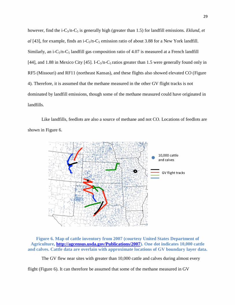
Like landfills, feedlots are also a source of methane and not CO. Locations of feedlots are
shown in Figure 6.
Figure 6. Map of cattle inventory from 2007 (courtesy United States Department of
Agriculture, http://agcensus.usda.gov/Publications/2007). One dot indicates 10,000 cattle
and calves. Cattle data are overlain with approximate locations of GV boundary layer data.
The GV flew near sites with greater than 10,000 cattle and calves during almost every
flight (Figure 6). It can therefore be assumed that some of the methane measured in GV

30
boundary layer runs could have been emitted from cattle and feedlots. Petron, et al [5], however,
notes that although feedlots emit methane, they do not emit a significant amount of n-pentane.
For this study, samples with both elevated methane and n-pentane were presumed to not be
significantly affected by emissions from feedlots.
3.1.3 Tracer and well proximity correlation plots for GV measurements within the boundary
layer
For each sample in the boundary layer, the number of nearby wells to the sampling
location were counted. By counting the number of nearby wells, individual concentration
measurements could then be evaluated as being more or less likely to be affected by oil and
natural gas fields. The case study (research flight 8 leg 1), for example, was chosen because
measurements within this low altitude leg were sampled near the most number of wells for the
campaign. A well is determined “nearby” based on the average direction of the wind and the
average wind speed. Stull [34] defines the boundary layer timescale as an hour or less, and this
timescale is used in the approximation of a radius that determines which wells may affect a
measurement at a specific location, calculated by:
where average wind speed is given in meters per second (Table 1) and 3600 is the number of
seconds per hour.
For a flight with highly variable wind direction (two standard deviations of the direction
is greater than 90 degrees), wells are counted as “nearby” if they are within a radius calculated as
given in the previous equation. An example of this calculation for one sample is shown in Figure

31
7 from flight 22, leg 1, where the wind speed averaged 5.76 m/s. The blue dots indicate
instrument sampling locations and the red circle is the area around the sample of interest with a
radius of about 20.7 km. Pink dots are active wells that are not within 20.7 km, whereas the black
dots indicate active wells determined as being “nearby.”
Figure 7. Example of number of "nearby" wells calculation for a flight with highly variable
wind direction (2σ > 90°). Blue dots indicate sampling locations. The red circle defines an
area around the sampling location where wells may be counted as being nearby. Pink dots
are wells not considered “nearby.” Black dots are wells considered “nearby.”
For a flight with less variable wind direction (two standard deviations does not exceed 90
degrees), a semi-circle of 180° instead defines the boundary of where wells can be considered
nearby. The radius of the semi-circle is the average wind speed in m/s multiplied by 3600 s to
calculate a distance out from the sampling location that could affect the measurement within one
hour. The semi-circle is oriented so that it is directed along the average wind direction measured
on the GV for that leg. Figure 8, for example, shows data from research flight 8, leg 2. The flight

32
had an average wind speed of 11.43 m/s and an average wind direction of 228.42°, or from the
southwest.
Figure 8. Example of number of "nearby" wells calculation for a flight with less variable
wind direction (2σ < 90°). Blue dots indicate sampling locations. The red semi-circle defines
an area around the sampling location where wells may be counted as being nearby. Pink
dots are wells not considered “nearby.” Black dots are wells considered “nearby.”
Results from the procedure described above are shown in Table 2.

33
Table 2. Number of nearby wells for GV boundary layer samples
Research Flight Number of
samples
Min. Number of
Wells
Max. Number of
Wells
Average ± 2σ
4 leg 1 15 0 29 4 ± 17
4 leg 2 2 24 27 25 ± 3
5 24 0 0 0 ± 0
6 48 0 127 40 ± 75
8 leg 1 80 0 930 79 ± 425
8 leg 2 32 0 42 12 ± 32
10 35 0 1 0 ± 1
11 39 0 0 0 ± 0
14 35 0 8 2 ± 4
17 34 0 1 0 ± 1
22 leg 1 107 0 296 23 ± 110
22 leg 2 61 0 141 18 ± 61
The following tracer plots were made to compare various atmospheric constituents with
their proximity to active oil and gas wells. Positive slopes in correlation plots indicate that the
two species may have been co-emitted. For the following correlation plots, data are shown from
all GV flights within the boundary layer Table 1. The color of each point in the plots corresponds
to the number of wells that are nearby that sampling location and is plotted on a logarithmic
scale.

34
Figure 9. Iso-Pentane vs. n-Pentane for GV flights within the boundary layer. Black line
shows slope of the Wattenberg Field in the Denver-Julesberg Basin (m = 0.86) [4]. Green
line shows slope of Ft. Worth Basin (m = 1.16) [46]. Color of each point corresponds to the
number of wells that were nearby the sampling location.
Figure 9 shows the iso-Pentane:n-Pentane ratio for GV boundary layer measurements
during the DC-3 campaign. Iso-Pentane (i-C5) and n-Pentane (n-C5) have comparable vapor
pressures, boiling points, and reaction rates with OH, so their concentrations will be similarly
affected as the two compounds are emitted and mixed into the boundary layer [4]. By plotting i-
C5 vs. n-C5, the importance of the effect of photochemistry of i-C5 and n-C5 concentrations is
minimized [4]. A slope of 0.86 pptv/pptv from the Gilman et al. [4] study sampled at Wattenberg
Field in the DJB and a slope of 1.16 pptv/pptv sampled at the Fort Worth Basin are plotted for
comparison to the measured values from the DC3 campaign. These two slopes are chosen as
many DC-3 GV flights flew near the DJB and the Fort Worth Basin and these slopes are the
maximum and minimum values considered for the two basins. The ratio, i-C5:n-C5, for different
reservoirs in the DC3 observation regions range from about 0.86 to 1.16 (Gilman et al. [4], Hill

35
et al. [49], Rodriguez [48]), whereas air strongly influenced by gasoline-related emissions will
have a higher ratio near 2.3-3.8.
Iso-pentane vs. n-pentane is shown here to compare the ratio to the sample’s proximity to
oil and gas wells. The data from the DC3 campaign show a strong correlation for all flights with
a correlation of r2 = 0.98. Dark red markers showing measurements close to over 100 active oil
and gas wells fall on the DJB slope and are from research flight 8 leg 1 near Denver and
northeast Colorado. Other measurements that are close to about 10 wells generally fall between
the two slopes. Points with slopes greater than 1.16 have lower concentrations of n-Pentane (less
than 400 pptv) and are near 10 or fewer active oil and gas wells. There are, however, points with
fewer than 10 active oil and gas wells that fall within the two slopes and some closer to 0.86
pptv/pptv. More research would need to be conducted on these samples, but it suggests that the
ratio is not a definitive way to identify oil and gas field emissions influence on a measurement.

36
Figure 10. CO vs. Methane measurements for GV flights within the boundary layer. Gray
line indicates correlation slope for all measurements. Color of each point corresponds to
the number of wells that are nearby the sampling location.
CO and methane measurements are compared in Figure 10 to investigate the possibility
of the two species being co-emitted. Sources of tropospheric methane include release from coal
mining and fossil fuel usage (110 ± 45 Tg yr-1
) [11]. Methane could be correlated with CO, also
a potential product of fossil fuel combustion, so a positive correlation implies that the air
sampled is strongly influenced by combustion. Figure 10 shows some structure to the
methane/CO ratio with a correlation of r2 = 0.54 and a positive slope of 1.40. Measurements near
over 20 wells generally show enhancements in methane that are not seen in CO, like the red
points at 105 ppbv CO corresponding to RF8 leg 1 in Colorado, the yellow points around 130
ppbv CO corresponding to RF6 in Texas, or the green points around 140 ppbv CO corresponding
to RF22 leg 1 in Texas. These three spikes in methane but not in CO sampled near over 20 wells
may indicate that the enhanced methane is not co-emitted with CO.

37
Methane vs. benzene and CO vs. benzene are shown next to each other to compare
possible sources of benzene. A major source of methane is emission from natural gas systems,
emitting 144.7 Tg CO2 equivalent [47]. Benzene has also been found to be emitted from oil and
natural gas fields, which may be a non-negligible source of benzene in the Colorado Front Range
[5]. CO and benzene both have a primary source from vehicular emissions [13] [19]. A strong
correlation between the two compounds would therefore indicate that it is likely the species were
co-emitted from motor vehicle combustion. As benzene can be emitted by oil and natural gas
fields or fossil fuel combustion, benzene is plotted with methane and CO to investigate a possible
correlation between the two tracers.
Methane vs. benzene is plotted on the left in Figure 11. The two tracers are positively
correlated (r2 = 0.33, slope = 0.38). The six green points around 1925-1975 ppbv of methane and
80-100 pptv of benzene are sampled during research flight 22, leg 1 in northern Texas near over
Figure 11. Methane vs. Benzene (left) and CO vs. Benzene (right) for GV flights within the boundary
layer. Gray line indicates correlation slopes for all measurements. Color of each point corresponds to
the number of wells that are nearby the sampling location.
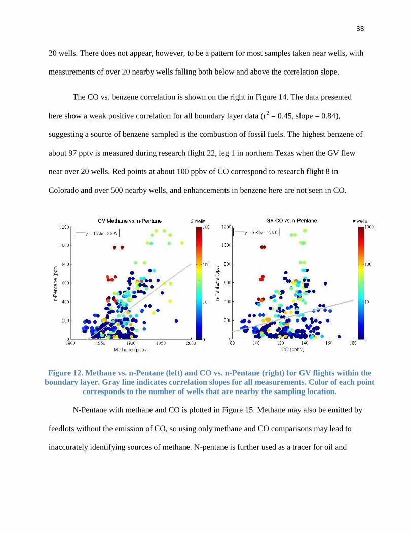
38
20 wells. There does not appear, however, to be a pattern for most samples taken near wells, with
measurements of over 20 nearby wells falling both below and above the correlation slope.
The CO vs. benzene correlation is shown on the right in Figure 14. The data presented
here show a weak positive correlation for all boundary layer data (r2 = 0.45, slope = 0.84),
suggesting a source of benzene sampled is the combustion of fossil fuels. The highest benzene of
about 97 pptv is measured during research flight 22, leg 1 in northern Texas when the GV flew
near over 20 wells. Red points at about 100 ppbv of CO correspond to research flight 8 in
Colorado and over 500 nearby wells, and enhancements in benzene here are not seen in CO.
N-Pentane with methane and CO is plotted in Figure 15. Methane may also be emitted by
feedlots without the emission of CO, so using only methane and CO comparisons may lead to
inaccurately identifying sources of methane. N-pentane is further used as a tracer for oil and
Figure 12. Methane vs. n-Pentane (left) and CO vs. n-Pentane (right) for GV flights within the
boundary layer. Gray line indicates correlation slopes for all measurements. Color of each point
corresponds to the number of wells that are nearby the sampling location.

39
natural gas wells here because the study by Petron, et al. [5] finds that feedlots emit lighter
alkanes but do not substantially affect the concentrations of n-pentane.
Methane and n-pentane are weakly positively correlated, (r2 = 0.37, slope = 4.7). Samples
with the most methane and n-Pentane are measured near about 20 wells in northern Texas in
research flight 22. Red points from research flight 8 in Colorado show high levels of n-Pentane,
although methane is measured at about 1860 ppbv, which is lower than the 1900 ppbv used as
the threshold for this study in determining a concentration to be elevated.
CO vs. n-pentane in Figure 12 has much weaker correlation than methane (r2 = 0.05)
suggesting that the n-pentane measured during the DC-3 campaign did not have a strong
common source with CO. Red data points corresponding to research flight 8 leg 1 spike at about
100 ppbv of CO. Simarly, green data points spike at about 140 pptv of CO and correspond to
research flight 22 leg 1. These measurements sampled in the proximity of over 10 oil and gas
wells show enhancements in n-Pentane that are not seen in CO, indicating that the two species
are likely not co-emitted for these samples.
3.1.4 Testing for correlation between proximity to wells and tracer data
Boundary layer tracer data from GV flights are tested for correlation with proximity to
wells using the method outlined by Guilford and Fruchter [51] using Student’s t distribution. A
two-tailed test is performed with a null hypothesis that ρ (the sample correlation) is equal to zero.
If ρ=0, then t can be estimated with the formula:

40
where N is the sample size, (N-2) is the degrees of freedom with two degrees lost in the two
datasets tested for correlation, and r is defined by the Pearson-r formula:
where x and y are the sample deviations from their respective means, N is the sample size, and Sx
and Sy are the standard deviations of X and Y.
Confidence intervals are determined following a method outlined in Hays [52]:
where Z is the Fisher r-to-Z transformation for a sample, ⁄ is the cut-off value for the upper
α/2 proportion in a normal distribution, N is the number of samples, and is the Fisher r-to-Z
transformation for the population. The interval is then transformed back to the corresponding
interval for . The Fisher r-to-Z transformation is given by:
Table 3 shows the two-tailed test results on correlations between CO, methane, n-
pentane, and benzene. The “campaign” test uses all boundary layer data. Individual flights with
more than one nearby oil well are also tested against these same tracers. N is the sample size, r

41
and t are calculated from the equations shown above, “95%CI” is the 95% confidence interval
for r, “%sig” is the level of significance in rejecting the null hypothesis, ρ=0. The null
hypothesis is not rejected in tests with significance over 10%, indicated by a blank cell. CO data
for RF4 are marked with bad data flags and are not used for hypothesis testing.

42
Table 3. Student’s t-test results for correlation between tracers and proximity to active oil and gas wells. Individual flight test
results for legs that flew near more than one active well
N
n-Pentane Methane Benzene
r t 95% CI %sig r t 95% CI %sig r t 95% CI %sig
Campaign 515 0.321 7.701 0.25 to 0.40 0.1% 0.061 1.390 -0.25 to 0.15 -0.124 -2.825 -0.21 to -0.04 1.0%
RF4 15 -0.457 -1.851 -0.78 to -0.05 10% -0.091 -0.330 -0.56 to 0.42 -0.027 -0.096 -0.52 to 0.48
RF6 48 0.003 0.017 -0.28 to 0.29 0.248 1.738 -0.04 to 0.50 10% -0.208 -1.443 -0.47 to 0.08
RF8 leg 1 80 0.760 10.316 0.65 to 0.84 0.1% 0.558 5.943 0.39 to 0.69 0.1% 0.376 3.588 0.17 to 0.55 0.1%
RF8 leg 2 32 -0.453 -2.783 -0.69 to -0.13 1% -0.579 -3.892 -0.77 to -0.29 0.1% -0.478 -2.980 -0.71 to -0.16 1%
RF14 35 0.282 1.688 -0.06 to 0.56 0.223 1.316 -0.12 to 0.52 0.211 1.241 -0.13 to 0.51
RF22 leg 1 107 0.327 3.511 0.14 to 0.49 0.1% 0.107 1.087 -0.09 to 0.29 0.252 2.641 0.06 to 0.42 2%
RF22 leg 2 61 0.059 0.457 -0.20 to 0.30 0.024 0.180 -0.23 to 0.27 0.150 1.161 -0.11 to 0.39
N
CO Ozone
r t 95% CI %sig r t 95% CI %sig
Campaign 515 -0.120 -2.731 -0.20 to -0.03 1.0% -0.070 -1.586 -0.16 to 0.02
RF4 15 N/A N/A N/A 0.480 1.972 -0.02 to 0.79 10%
RF6 48 -0.146 -1.000 -0.41 to 0.15 0.139 0.955 -0.15 to 0.41
RF8 leg 1 80 -0.218 -1.973 -0.42 to 0.00 10% -0.296 -2.740 -0.48 to -0.08 1%
RF8 leg 2 32 -0.414 -2.491 -0.67 to -0.08 2% -0.584 -3.941 -0.78 to -0.30 0.1%
RF14 35 0.088 0.508 -0.25 to 0.41 0.264 1.571 -0.08 to 0.55
RF22 leg 1 107 -0.293 -3.107 -0.46 to -0.11 1% -0.518 -6.151 -0.65 to -0.36 0.1%
RF22 leg 2 61 0.082 0.633 -0.17 to 0.33 0.162 1.257 -0.09 to 0.40

43
For all GV DC-3 data within the boundary layer, n-pentane is positively correlated with
the proximity to natural oil and gas wells. N-pentane has a level of significance at 0.1% while the
test on methane failed to reject ρ=0. This may be due to n-pentane having shorter lifetimes
(about 5 days [48]) than methane (9 years [6]), so gradients in n-pentane are more pronounced.
By contrast, benzene and CO resulted in a rejection of the null hypothesis for negative
correlations. CO and benzene are primarily emitted from combustion and is not significantly
enhanced by oil and gas wells [5]. From the active well plots in Figure 3 and Figure 4, cities like
Denver and Oklahoma City are located near clusters of active wells, but within them. For
example, the southernmost well in the DJB lies about 26.6 km to the north of Denver, and the
closest well to Oklahoma City is 201.4 km. This may explain why CO decreases with decreasing
number of nearby wells. In a study by Gilman, et al [4], emissions of VOCs from oil and gas
operations have been found to be related to high ambient ozone levels. Ozone, however, failed to
reject ρ=0. One reason for this, like CO, may be that enhancements in ozone from urban
emissions may dominate the measurements near oil and gas wells.
The test is performed on individual flights that flew near more than one well. All flights
except research flight 8 leg 1 show correlations that were not expected based on previous studies
cited within this paper (positive correlations with n-pentane, methane, and benzene). RF8 legs 1
and 2 and RF22 leg 1, however reject the null hypothesis for the positive correlations of n-
pentane, and reject the null for negative correlations with CO and ozone. RF8 leg 1 (the case
flight for this study) and RF22 leg 1 measurements occurred near the most wells, with a
maximum count of 930 and 296 wells, respectively. This may suggest why these two particular
flights show positive correlation of n-pentane with oil and gas wells. RF8, leg 1 is used for the
case study because it flew near the most wells. RF22, though it flew near many wells, has

44
measurements of some of the highest concentrations of CO sampled for the campaign in GV
boundary layer, suggesting the air is strongly influenced by combustion, possibly complicating
the identification of contributions from oil and gas wells.
3.2 1 June 2012 (GV-RF8), Colorado low altitude leg case study [24]
On 1 June 2012, the GV (RF8) and the DC8 (RF8) deployed from Salina, Kansas to
characterize emissions sources in Colorado and a convective storm near Oklahoma and Texas
(flight track shown in Figure 16). The GV took off around 19:50 UTC and flew in three
intercomparison legs with the DC8 en route to Colorado. After the intercomparisons, the GV
flew along the Colorado foothills near Denver to sample urban emissions. The GV’s potential
temperature sounding into the lower altitude leg at about 2.8 km shows a boundary layer near
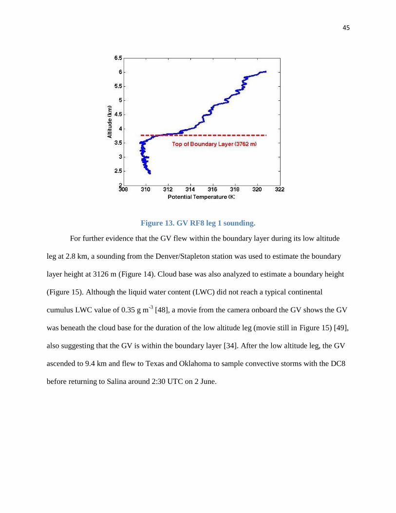
3762 m (Figure 13).
45
Figure 13. GV RF8 leg 1 sounding.
For further evidence that the GV flew within the boundary layer during its low altitude
leg at 2.8 km, a sounding from the Denver/Stapleton station was used to estimate the boundary
layer height at 3126 m (Figure 14). Cloud base was also analyzed to estimate a boundary height
(Figure 15). Although the liquid water content (LWC) did not reach a typical continental
cumulus LWC value of 0.35 g m-3
[48], a movie from the camera onboard the GV shows the GV
was beneath the cloud base for the duration of the low altitude leg (movie still in Figure 15) [49],
also suggesting that the GV is within the boundary layer [34]. After the low altitude leg, the GV
ascended to 9.4 km and flew to Texas and Oklahoma to sample convective storms with the DC8
before returning to Salina around 2:30 UTC on 2 June.

46
Figure 14. Denver station sounding 2 June, 2012 at 00:00 UTC [50]. Red dotted line at
3126m indicates the top of the boundary layer.
Figure 15. GV forward camera showing the cloud base (left), picture taken during research
flight 8 on June 1 at 22:36 UTC [51]. Liquid water content (right) with arrows indicating
start and end of leg 1. Blue line is GV altitude for RF8, green is liquid water content.
The first low altitude leg of the 1 June flight was chosen as a case flight to study oil and
gas field emissions because the GV flew near over 500 active oil and gas wells, more than any

47
other low altitude leg in the campaign by the GV and was likely to have sampled air influenced
by oil and gas wells. As noted in Table 1, mean wind speed for RF8 leg 1 was 3.84 m/s with
highly variable winds, so wells were counted as “nearby” if they were within a 13.8 km radius of
the location of the measurement. Nearby active wells in research flight 8 correspond to the
Denver-Julesberg Basin (Figure 1).
Figure 16. Flight track for 1 June 2012 (GV research flight 8). Green dots show locations of
active oil and gas wells [37]. Black line shows the low altitude leg analyzed in the case
study. Red line shows the rest of the flight.
The back trajectories in Figure 17 were created by HYSPLIT using the GDAS archive.
Heights are 2430 for Figure 17A, 2730 m for Figure 17B, and 2730 for Figure 17C,
corresponding to the approximate altitude of the GV and the start, middle and end of low altitude
leg. Boundary layer heights are the average heights provided by HYSPLIT for each ensemble.

48
Figure 17. HYSPLIT back trajectories using GDAS archive data for GV research flight 8.
Ensemble plots are made for the start (A), middle (B) and end (C) of the low altitude leg
used in the 1 June case study.
Back trajectories show that the air sampled on the GV may be influenced by sources to
the northwest of the measurements locations. Basins to the northwest include Greater Green
River Basin and Park Basin. The boundary layer heights do not agree with the boundary layer
height estimated from the GV sounding (Figure 13) and are at a lower altitude than the GV flew
for this leg. Back trajectories are shown in (Figure 18) that have an input altitude within the

49
boundary layer according to the HYSPLIT model (chosen to be 1500 m here) to determine if the
trajectory varies enough to show air influenced from another direction.
Figure 18. HYSPLIT back trajectories using GDAS archive data for GV research flight 8.
Ensemble plots are made for the start (A), middle (B) and end (C) of the low altitude leg
used in the 1 June case study with altitudes at 1500 m.
Back trajectories shown in Figure 18 still show the air coming from approximately the
northwest. Though the boundary layer heights disagree between the Denver sounding and

50
HYSPLIT, back trajectories for altitudes corresponding to the GV (Figure 17) and altitudes
within the HYSPLIT boundary layer (Figure 18) both show air coming from the northwest. For
the purposes of this study, it was therefore assumed that the air sampled in research flight 8, leg 1
was influenced by either the surface or sources to the northwest.
3.2.1 Tracer and nearby well correlation plots for research flight 8 case study
Similar plots to section 3.1.2 were made using only data from research flight 8, low
altitude leg 1. The GV flew close to Denver and may have sampled air influenced by urban
sources. To investigate the possible contributions of urban and oil and gas wells, plots show
proximity to active wells as wells as proximity to Denver. Data points in Figure 19 and Figure 20
represent the same samples, but the color of each point represents either the proximity to number
of wells (plots on left) or proximity to Denver (plots on right). Data shown are measured within
the boundary layer along the Colorado Front Range (black line in Figure 16) and boundary layer
height is determined from the GV sounding. Correlation slopes are provided for each comparison
for measurements near over 291 wells (the average of the number of nearby wells plus one
standard deviation) and measurements less than 26 km from Denver (average distance from
Denver minus one standard deviation) to show the difference in slopes between two possible
sources.
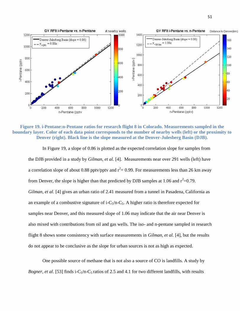
51
In Figure 19, a slope of 0.86 is plotted as the expected correlation slope for samples from
the DJB provided in a study by Gilman, et al. [4]. Measurements near over 291 wells (left) have
a correlation slope of about 0.88 pptv/pptv and r2= 0.99. For measurements less than 26 km away
from Denver, the slope is higher than that predicted by DJB samples at 1.06 and r2=0.79.
Gilman, et al. [4] gives an urban ratio of 2.41 measured from a tunnel in Pasadena, California as
an example of a combustive signature of i-C5/n-C5. A higher ratio is therefore expected for
samples near Denver, and this measured slope of 1.06 may indicate that the air near Denver is
also mixed with contributions from oil and gas wells. The iso- and n-pentane sampled in research
flight 8 shows some consistency with surface measurements in Gilman, et al. [4], but the results
do not appear to be conclusive as the slope for urban sources is not as high as expected.
One possible source of methane that is not also a source of CO is landfills. A study by
Bogner, et al. [53] finds i-C5/n-C5 ratios of 2.5 and 4.1 for two different landfills, with results
Figure 19. i-Pentane:n-Pentane ratios for research flight 8 in Colorado. Measurements sampled in the
boundary layer. Color of each data point corresponds to the number of nearby wells (left) or the proximity to
Denver (right). Black line is the slope measured at the Denver-Julesberg Basin (DJB).

52
comparable to a similar study at a landfill in New York. The maximum i-C5/n-C5 value for this
leg is found to be 1.42, a lower ratio than what is expected from landfills, suggesting that
landfills do not significantly affect the tracer concentrations measured in research flight 8 in
Colorado.
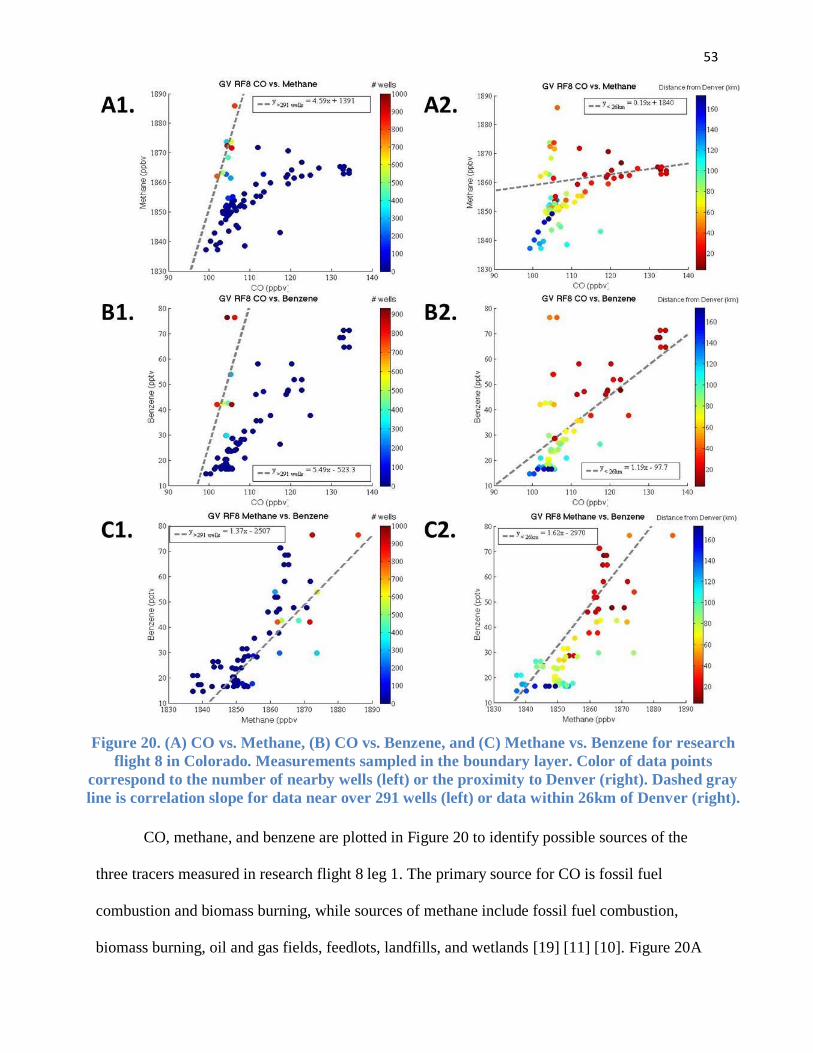
53
CO, methane, and benzene are plotted in Figure 20 to identify possible sources of the
three tracers measured in research flight 8 leg 1. The primary source for CO is fossil fuel
combustion and biomass burning, while sources of methane include fossil fuel combustion,
biomass burning, oil and gas fields, feedlots, landfills, and wetlands [19] [11] [10]. Figure 20A
Figure 20. (A) CO vs. Methane, (B) CO vs. Benzene, and (C) Methane vs. Benzene for research
flight 8 in Colorado. Measurements sampled in the boundary layer. Color of data points
correspond to the number of nearby wells (left) or the proximity to Denver (right). Dashed gray
line is correlation slope for data near over 291 wells (left) or data within 26km of Denver (right).

54
shows two possible correlation slopes for methane and CO, with one at y = 4.59x+1391 (r2=
0.15) for samples near over 291 wells (A1), and y = 0.19x+1840 (r2= 0.57) for samples within 26
km of Denver (A2). The two slopes suggest at least two different sources of methane and/or CO.
The spike at about 104 ppbv of CO has enhancements in methane that are not seen with
enhancements in CO, which suggests a source of methane that is not a strong source of CO: oil
and gas fields, feedlots, landfills, or wetlands. For the CO vs. methane slope more closely
associated with the slope given by samples near Denver (A2), enhancements are seen in both CO
and methane, indicating a source that emits both of these tracers: biomass burning or fossil fuel
combustion.
Figure 20A is plotted next to Figure 20B and C to further attempt to identify a possible
source for CO, methane, and benzene. In Figure 20B1, a similar spike is seen at about 104 ppbv
of CO as was seen in Fig. 20A1 with many of these measurements taken near over 300 wells.
This same spike may indicate that there is a source of methane and benzene that does not also
significantly enhance CO. As mentioned in the previous paragraph, possible sources for methane
that do not also significantly affect concentrations of CO are oil and gas fields, feedlots, landfills,
and wetlands. Sources of benzene, however, include vehicular emissions (also a source for CO)
and oil and gas fields [5] [13]. Oil and gas fields, therefore, can emit benzene and methane
without emitting CO, suggesting that measurements shown at 104 ppbv CO may be influenced
by oil and gas fields and their proximity to over 300 wells further supports this idea.
Figure 20C shows methane vs. benzene to show the correlation of the two tracers. In the
plot that shows nearby wells (C1), the two data points with the highest concentration of methane
and benzene are near over 1500 wells. In Fig. 20C2, lowest values of benzene are typically
furthest away from Denver while highest values are closer (correlation test in Table 3), which

55
might suggest proximity has some importance in the concentration of benzene, but the spike
from Figure 20B at 104 ppbv CO still suggests that the source of the benzene measured in this
spike is likely not from a combustive source.
Figure 21. (A) CO vs. n-Pentane and (C) Methane vs. n-Pentane for research flight 8 in
Colorado. Measurements sampled in the boundary layer. Color of each data point
corresponds to the number of nearby wells (left) or the proximity to Denver (right). Dashed
gray line is correlation slope for data near over 291 wells (left) or data within 26km of
Denver (right).
CO and methane are plotted against n-pentane in Figure 21 to attempt to exclude feedlots
from sources of methane as a major contributor to the concentration of methane measured during
research flight 8 leg 1. Sources of n-pentane include fossil fuel combustion and oil and gas fields,
but feedlots do not significantly affect the concentrations of n-pentane [5]. Figure 21A shows CO

56
vs, n-pentane to attempt to identify n-pentane that may be from fossil fuel combustion. The spike
at 104 ppbv CO and the group of data points from about 0-400 pptv n-pentane and about 100-
135 ppbv CO suggests that there are at least two sources of n-pentane. The spike at 104 ppbv CO
has the most nearby wells of the data presented here, and strong enhancements in n-pentane are
not seen in CO, indicating that the data at about 104 ppbv CO and over 400 pptv n-pentane are
likely not from a combustive source. The less steep slope from 100-135 ppbv CO and 0-400
pptv, however, shows enhancements in CO as well as n-pentane. The increasing proximity to
Denver also suggests that the data along this slope are likely influenced by combustive sources.
One possible source of methane that would not also emit CO is feedlots, but a study by
Petron, et al. [5] finds that feedlots did not enhance the concentrations of n-pentane. The two
data points in Figure 21B1 with over 1500 wells that lie farthest below the best-fit line in B1, for
example, have some of the highest methane for this flight leg, but n-pentane is at about 400 pptv,
the same value for some samples not collected near any active wells. With enhanced methane,
and n-pentane not as enhanced as the other data points near as many wells, these data points may
indicated contributions from feedlots. For other data points near over 291 wells, n-pentane values
lie close to or above the correlation slope for Fig. 21B1, suggesting that the methane sampled at
the same time is likely from a source that also emits n-pentane.
Figure 21 B2 suggests that n-pentane generally increases with proximity to Denver
(correlation test in Table 3). Some correlation with CO and Methane in proximity to Denver
indicates that some of the n-pentane measured in research flight 8 is from fossil fuel combustion.

57
3.2.2 Testing for correlation for research flight 8 case study
As in section 3.1.3, a similar hypothesis test is performed on research flight 8, leg 1 for
correlation of tracers to the proximity of Denver. T-tests are performed using the null hypothesis,
ρ=0. Data from 3.1.3 for correlation with wells are shown again here to compare with results
from Denver in Table 4. N is the number of samples, r and t are calculated from equations in
3.1.3, 95%CI is the 95% confidence interval for r, and %sig is the level of significance for the
test.

58
Table 4. Hypothesis test results for case study. Tracers are tested for correlation with proximity to wells and to Denver
N
n-Pentane Methane Benzene
r t 95% CI %sig r t 95% CI %sig r t 95% CI %sig
Wells 80 0.760 10.316 0.65 to 0.84 0.1% 0.558 5.943 0.39 to 0.69 0.1% 0.376 3.588 0.17 to 0.55 0.1%
Denver 80 0.289 5.625 0.07 to 0.48 0.1% 0.664 7.836 0.52 to 0.77 0.1% 0.773 10.750 0.67 to 0.85 0.1%
N
CO Ozone
r t 95% CI %sig r t 95% CI %sig
Wells 80 -0.218 -1.973 -0.42 to 0.00 10% -0.296 -2.740 -0.48 to -0.08 1%
Denver 80 0.656 7.678 0.51 to 0.77 0.1% 0.618 6.935 0.46 to 0.74 0.1%

59
The null hypothesis is rejected for a positive correlation between wells and n-pentane,
methane, and benzene. CO and ozone reject the null hypothesis for a negative correlation
between the tracers and oil and gas wells. This indicates that oil and gas wells may be a
significant source of n-pentane, methane, and benzene but not CO or ozone. The results here
agree with the results expected from other studies cited within this paper.
With respect to Denver, all tests reject the null hypothesis for a positive correlation. N-
pentane is correlated with proximity to Denver with a correlation coefficient of 0.07 to 0.48. This
is weaker than the interval for wells, 0.65 to 0.84, suggesting that oil and gas wells may be a
more significant source of n-pentane than urban sources. Methane is also found to likely be
correlated with proximity to Denver, but with a correlation coefficient near that of active wells
(0.66 and 0.56, respectively), indicating that both sources may be significant. Correlation with
benzene also rejects the null hypothesis with a confidence interval of 0.67 to 0.85, which is a
stronger correlation than that given by proximity to wells (0.17 – 0.55). Urban sources are
therefore likely to emit more benzene than oil and gas wells, although Figure 20 suggests that
there are at least two sources of benzene for the samples taken with research flight 8.
CO and ozone also rejected the null for a positive correlation for proximity to Denver
while the two tracers were found to be negatively correlated with proximity to oil and gas wells.
The CO result suggests that Denver is a large source of combustion emissions, and some of the
ozone measured is due to in-situ photochemical reactions with VOCs, NOx, and methane as the
concentrations of ozone may be correlated with proximity to an urban area [23].

60
4. Conclusions
This study analyzes oil and gas field tracers as well as urban chemical tracers for
measurements taken in the boundary layer on the Gulfstream V in the DC-3 campaign. Data was
initially filtered for samples within the boundary layer using in situ measurements of potential
temperature taken onboard the GV. Proximity to wells was also considered in assessing the
possibility of influence from oil and gas field emissions on the air sampled. Finally, the study
presents a case study of a flight on 1 June 2012 from the DC3 campaign. Measurements
presented here are from instruments onboard the GV, sampling at altitudes of 2.4 km to 2.7 km
over an area of oil and gas fields of the Denver-Julesberg Basin in northern Colorado.
Comparisons between urban and oil and gas field tracers suggest the air sample during this flight
is influenced by oil and gas fields.
Hypothesis testing of both the case study and flights that sampled near the most wells in
the campaign suggest that it cannot be concluded that high methane and high pentane were not
elevated by oil and gas field emissions. For all GV data sampled in the boundary layer, n-pentane
was found to be positively correlated with the proximity to natural oil and gas wells, whereas
methane yielded inconclusive results. It is possible that the shorter lifetime of n-pentane
compared to methane (about five days compared to nine years) would cause there to be a
stronger correlation between n-pentane and its source. Benzene and CO resulted in a rejection of
the null hypothesis for negative correlations for GV flights. CO and benzene are primarily urban
tracers that are not significantly enhanced by oil and gas wells, and oil and gas fields in the
region studied are not located within urban centers, which may suggest why benzene and CO
decrease in concentration as the proximity of the sample to wells increases. Ozone also failed to
reject the null hypothesis. Emissions from oil and gas wells can be related to high ozone

61
concentrations [4], but ozone is also influenced by urban sources, and these urban sources may
be more significant in enhancing the concentration of ozone than oil and gas wells.
Hypothesis testing for individual flights reveal that only RF8 leg 1 and 2, and RF22 leg 1
reject the null for negative correlations between proximity to wells and CO and ozone. RF8 leg 1
and RF22 leg 1 were the two flight legs with the highest number of nearby oil and gas wells
(maximum: 930 and 296 wells, respectively) and may be why results from the two flights
indicate a positive correlation between n-pentane and active wells.
To select a case study, concentrations for i-C5/n-C5, methane, n-pentane, benzene, CO,
and ozone were plotted along flight tracks. Flights with high methane and high n-pentane were
considered for the case study. RF8 leg 1 and RF22 leg 2 were found to have high n-pentane.
RF10 and RF8 leg 2 also had i-C5/n-C5 ratios near one and back trajectories that showed air
coming from the Denver-Julesberg Basin and the Fort Worth basin, respectively, also suggesting
possible influence from oil and natural gas wells. Next, research flights are further analyzed to
find the flights near the most oil and gas wells for better statistical analysis. RF8 leg 1 was
chosen as the case study because it had high n-pentane. The G-V flew near the most oil and gas
wells and an urban area in RF8 leg 1, which further allowed for the comparison of concentrations
of oil and gas tracers and urban tracers along the flight track.
For the low level transect of the 1 June flight (RF8 leg 1), the i-C5/n-C5 ratio had a slope
of 0.88 for samples near over 291 wells, and 1.04 for samples within 26 km of Denver. The slope
for proximity to Denver is much less than the ratio for gasoline related sources (slope = 2.3 –
3.0) [4], but the oil and gas slope falls close to surface measurements of the Denver-Julesburg
Basin (0.86). Benzene, a known carcinogen with surface sources primarily from vehicular
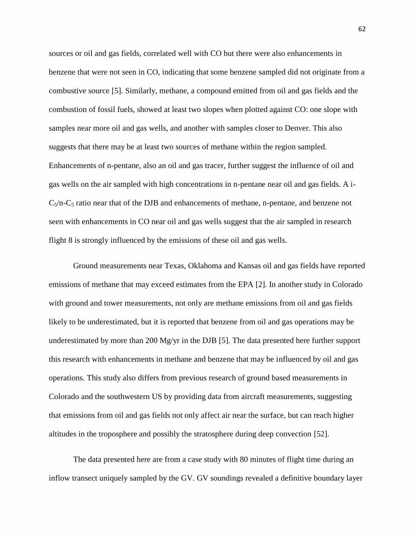
62
sources or oil and gas fields, correlated well with CO but there were also enhancements in
benzene that were not seen in CO, indicating that some benzene sampled did not originate from a
combustive source [5]. Similarly, methane, a compound emitted from oil and gas fields and the
combustion of fossil fuels, showed at least two slopes when plotted against CO: one slope with
samples near more oil and gas wells, and another with samples closer to Denver. This also
suggests that there may be at least two sources of methane within the region sampled.
Enhancements of n-pentane, also an oil and gas tracer, further suggest the influence of oil and
gas wells on the air sampled with high concentrations in n-pentane near oil and gas fields. A i-
C5/n-C5 ratio near that of the DJB and enhancements of methane, n-pentane, and benzene not
seen with enhancements in CO near oil and gas wells suggest that the air sampled in research
flight 8 is strongly influenced by the emissions of these oil and gas wells.
Ground measurements near Texas, Oklahoma and Kansas oil and gas fields have reported
emissions of methane that may exceed estimates from the EPA [2]. In another study in Colorado
with ground and tower measurements, not only are methane emissions from oil and gas fields
likely to be underestimated, but it is reported that benzene from oil and gas operations may be
underestimated by more than 200 Mg/yr in the DJB [5]. The data presented here further support
this research with enhancements in methane and benzene that may be influenced by oil and gas
operations. This study also differs from previous research of ground based measurements in
Colorado and the southwestern US by providing data from aircraft measurements, suggesting
that emissions from oil and gas fields not only affect air near the surface, but can reach higher
altitudes in the troposphere and possibly the stratosphere during deep convection [52].
The data presented here are from a case study with 80 minutes of flight time during an
inflow transect uniquely sampled by the GV. GV soundings revealed a definitive boundary layer

63
and a camera onboard that showed the flight leg occurring beneath the cloud base. It is therefore
likely that the flight leg was conducted within the boundary layer and its location over the
Denver-Julesberg basin suggests that the air sampled may have been influenced by oil and gas
wells.
Because the GV usually flew in outflow regions, there are a relatively small number of
research flights from the DC3 with boundary layer measurements from the GV. The DC8,
however, flew several legs in inflow regions at low altitudes, likely within the boundary layer.
Instruments onboard the DC8 also measured other alkanes, such as ethane and propane, which
can be used as other tracers for oil and gas fields [5]. Further research into the emissions of
methane and benzene from oil and natural gas fields measured during the DC3 campaign could
therefore investigate measurements made during DC3 flights.
Other future work may involve source apportionment for enhancements of methane
observed during the DC3 campaign. Higher concentrations of methane sampled over the region
of the US covered by the DC3 campaign may also be due to landfills, domestic ruminants, and
wetlands. These sources would emit methane without the tracers discussed in this study from
combustion or oil and natural gas fields. N-pentane is used in this study to exclude feedlots as a
significant source of methane, and the i-C5/n-C5 ratio is used in excluding landfills. Stronger
conclusions may be made, however, with more tracers or identifying locations of landfills and
feedlots and testing against the proximity to these locations. In addition, GV research flight 22
(30 June 2012), flew at less than 1.9 km for 1.75 hours over an area with many active wells and
further analysis would be required to investigate the contribution of oil and natural gas emissions
on the air sampled. During the 30 June flight, however, measurements of i-pentane, n-pentane,
CO, O3, and CH4 indicate a complicated mixture of sources.

64
Works Cited
[1] F.-Y. Liang, M. Ryvak, S. Sayeed and N. Zhao, "The role of natural gas gas a primary fuel in the near
future, including comparisons of acquisition, transmission, and waste handling costs of as with
competitive alternatives," Chemistry Central, vol. 6, no. S4, 2012.
[2] A. S. Katzenstein, L. A. Doezema, I. J. Simpson, D. R. Blake and F. S. Rowland, "Extensive regional
atmospheric hydrobarbon pollution in the southwestern United States," Proceedings of the
National Academy of Sciences of the United States of America, vol. 100, no. 21, pp. 11975-11979,
2003.
[3] S. Pacala and R. Socolow, "Stabilization Wedges: Solving the Climate Problem for the Next 50 Years
with Current Technologies," Science, vol. 305, no. 5686, pp. 968-972, 2004.
[4] J. B. Gilman, B. M. Lerner, W. C. Kuster and J. A. de Guow, "Source signature of volatile organic
compounds from oil and natural gas operations in northeastern Colorado," Environmental Science
and Technology, vol. 47, pp. 1297-1305, 2013.
[5] G. Petron, G. Frost, B. R. Miller and e. al., "Hydrocarbon emissions characterization in the Colorado
Front Range: A pilot study," Journal of Geophysical Research, vol. 117, no. D04304, 2012.
[6] S. A. Montzka, E. J. Dlugokencky and J. H. Butler, "Non-CO2 greenhouse gases and climate change,"
Nature, vol. 476, pp. 43-50, 2011.
[7] "IPCC Fourth Assessment Report: Climate Change 2007," WMO, 2007.
[8] P. Bousquet, P. Ciais, J. B. Miller, E. J. Dlugokencky, D. Hauglustaine, C. Prigent, G. R. Van der Werf,
P. Peylin, E. -G. Brunke, C. Carouge, R. L. Langenfelds, J. Lathiere, F. Papa, M. Ramonet, M. Schmidt,
L. Steele, S. Tyler and J. White, "Contribution of anthropogenic and natural sources to atmospheric
methane variability," Nature, vol. 443, pp. 439-443, 2006.
[9] M. Prather and D. Ehhalt, "Atmospheric Chemistry and Greenhouse Gases," in Working Group I:
The Scientific Basis, WMO, 2001.
[10] R. W. Howarth, R. Santoro and A. Ingraffea, "Methane and the greenhouse-gas footprint of natural
gas from shale formations," Climate Change, vol. 106, pp. 679-690, 2011.
[11] J. Lelieveld, P. J. Crutzen and F. J. Dentener, "Changing concentraion, lifetime and climate forcing of
atmospheric methane," Tellus, vol. 50B, pp. 128-150, 1998.
[12] R. W. Howarth, R. Santoro and A. Ingraffea, "Venting and leaking of methane from shale gas
development: response to Cathles et al.," Climatic Change, vol. 113, pp. 537-549, 2012.

65
[13] "Benzene: TEACH Chemical Summary," EPA, 2009.
[14] N. V. Heeb, A.-M. Forss, C. Bach, S. Reimann, A. Herzog and H. W. Jackle, "A comparison of
benzene, toluene, and C2-benzenes mixing ratios in automotive exhaust and in the suburban
atmosphere during the introduction of catalytic converter technology to the Swiss Car Fleet,"
Atmospheric Environment, vol. 34, pp. 3103-3116, 2000.
[15] R. Atkinson, "Gas-phase tropospheric chemistry of organic compounds: A review," Atmospheric
Environment, vol. 24A, no. 1, pp. 1-41, 1990.
[16] "Evaluation of Impacts to Underground Sources of Drinking Water by Hydraulic Fracturing to
Coalbed Methane Reservoirs, Final Report," Environmental Protection Agency, 2004.
[17] N. Yassaa, Y. M. Brahim, A. Cecinato and F. Marino, "Particulate n-alkanes, n-alkanoic acids and
polycyclic aromatic hydrocarbons in the atmosphere of Algiers City Area," Atmospheric
Environment, vol. 35, no. 10, pp. 1843-1851, 2001.
[18] D. J. Jacob, B. D. Field, E. M. Jin, I. Bey, L. Qinbin, J. A. Logan and R. M. Yantosca, "Atmospheric
budget of acetone," Journal of Geophysical Research, vol. 107, 2002.
[19] C. Clerbaux, D. P. Edwards, M. Deeter, L. Emmons, J. -F. Lamarque, X. T. Xue, S. T. Massie and J.
Gille, "Carbon monoxide pollution from cities and urban areas observed by the Terra/MOPITT
mission," Geophysical Research Letters, vol. 35, no. 3, 2008.
[20] P. A. Okken, "Methane leakage from natural gas," Energy Policy, vol. 3, pp. 202-204, 1990.
[21] D. J. McKee, Tropospheric ozone, Boca Raton: Lewis Publishers, 1993.
[22] J. H. Seinfeld and S. N. Pandis, Atmospheric Chemistry and Physics, Hoboken, NJ: John Wiley &
Sons, Inc, 2006.
[23] E. A. Ainsworth, C. Yendrek, S. Stitch, W. J. Collins and L. D. Emberson, "The effects of tropospheric
ozone on net primary production and implications for climate change," Annual Review of Plant
Biology, vol. 63, pp. 637-661, 2012.
[24] "DC3 Operations Plan," 28 April 2012.
[25] "Picarro G1301: Carbon Dioxide, Methane & Water Vapor Analyzer," Picarro, Sunnyvale, CA, 2009.
[26] Picarro, Inc, "Applications Note Atmospheric Monitoring," Picarro, Inc, 2013. [Online]. Available:
http://www.picarro.com/assets/docs/atmospheric_monitoring_app_note.pdf. [Accessed 25 April
2013].
66
[27] A. Volz and D. Kley, "A resonance-fluorescence instrument for the in-situ measurement of
atmospheric carbon monoxide," Journal of Atmospheric Chemistry, vol. 2, pp. 345-357, 1985.
[28] C. Gerbig, S. Schmitgen, D. Kley and A. Volz-Thomas, "An improved fast-response vacuum-UV
resonance fluorescence CO instrument," Journal of Geophysical Research, vol. 104, pp. 1699-1704,
1999.
[29] E. C. Apel, A. J. Hills, R. Lueb, S. Zindel, S. Eisele and D. D. Riemer, "A fast-GV/MS system to
measure C2 to C4 carbonyls and methanol aboard aircraft," Journal of Geophysical Research:
Atmospheres, vol. 108, no. D20, 2003.
[30] B. A. Ridley, F. E. Grahek and J. G. Walega, "A small, high-sensitivity, medium-response ozone
detector suitable for measurements from light aircraft," Journal of Atmospheric and Oceanic
Technology, vol. 9, pp. 142-148, 1991.
[31] C. Yi, K. J. Davis and B. W. Berger, "Long-Term Observations of the Dynamics of the Continental
Planetary Boundary Layer," Journal of Atmospheric Sciences, vol. 58, pp. 1288-1299, 2000.
[32] "DC3 Field Catalog: Radar Products, NEXRAD_3D_mosaic_map(06kft_CAPPI)," June 2012. [Online].
Available: http://catalog.eol.ucar.edu/cgi-
bin/dc3_2012/radar/prod_browse?platform=NEXRAD_3D_mosaic_map&prod=06kft_CAPPI&how
many=Use+Start%2FEnd+Dates+-
%3E&start=20120616&end=20120617&submit=retrieve+products. [Accessed 6 May 2013].
[33] Q. Youcan, J. Zhang and P. Zhang, "A real-time automated convective and sratiform precipitation
segregation algorithm in native radar coordinates," Quarterly Journal of the Royal Meteorological
Society, 2013.
[34] R. B. Stull, An Introduction to Boundary Layer Meteorology, Dordrecht: Kluwer Academic
Publishers, 1988.
[35] "Air Resources Laboratory - GDAS Data Archive," National Oceanic and Atmospheric
Administration, 8 January 2013. [Online]. Available: ready.arl.noaa.gov/gdas1.php. [Accessed 14
July 2013].
[36] Air Resources Laboratory, "HYSPLIT - Hybrid Single Particle Lagrangian Integrated Trajectory
Model," NOAA, 25 April 2013. [Online]. Available: http://ready.arl.noaa.gov/HYSPLIT.php.
[Accessed 7 May 2013].
[37] D. Manthos, "SkyTruth Drilling Alerts," SkyTruth, 14 November 2012. [Online]. Available:
http://frack.skytruth.org/fracking-chemical-database. [Accessed 18 April 2013].

67
[38] P. D. Jenden, K. D. Newell, I. R. Kaplan and W. L. Watney, "Composition and stable-isotope
geochemsitry of natural gases from Kansas, Midcontinent, USA," Chemical Geology, vol. 71, no. 1-
3, pp. 117-147, 1998.
[39] B. D. Berger and K. E. Anderson, Modern Petroleum: A basic primer of the industry, Tulsa,
Oklahoma: PennWell Publishing Company, 1992.
[40] B. D. Gage and D. L. Driskill, "Analysis of Natural Gases, 2002-2004," United States Department of
the Interior: Bureau of Land Management, 2005.
[41] J. J. Schauer, M. J. Kleeman, G. R. Cass and B. R. T. Simoneit, "Measurement of emissions from air
pollution sources. 5. C1-C32 organic compounds from gasoline-powered motor vehicles,"
Environment Science Technology, vol. 36, no. 6, pp. 1169-1180, 2002.
[42] V. E. Wittig, E. A. Ainsworth, S. L. Naidu, D. F. Karnosky and S. P. Long, "Quantifying the impact of
current and future tropospheric ozone on tree biomass, growth, physiology and biochemistry: a
quantitative meta-analysis," Global Change Biology, vol. 15, no. 2, pp. 396-424, 2009.
[43] B. Eklund, E. P. Anderson, B. L. Walker and D. B. Burrows, "Characterization of Landfill Gas
Composition at the Fresh Kills Municipal Solid-Waste Landfill," Environmental Science Technology,
vol. 32, no. 15, pp. 2233-2237, 1998.
[44] C. Schuetz, J. Bogner, J. Chanton, D. Blake, M. Morcet and P. Kjeldsen, "Comparative Oxidation and
Net Emissions of Methane and Selected Non-Methane Organic Compounds in landfill Cover Soils,"
Environmental Science Technology, vol. 37, no. 22, pp. 5150-5158, 2003.
[45] E. Vega, V. Mugica, R. Carmona and E. Valencia, "Hydrocarbon source apportionment in Mexico
City using the chemical mass balance receptor model," Atmospheric Environment, vol. 34, no. 24,
pp. 4121-4129, 2000.
[46] N. D. Rodriguez and R. P. Philp, "Geochemical characterization of gases from the Mississippian
Barnett Shale, Fort Worth Basin, Texas," The American Association of Petroleum Geologists, vol. 94,
no. 11, pp. 1641-1656, 2010.
[47] U.S. Environmental Protection Agency, "Inventory of U.S. Greenhouse Gas Emissions and Sinks:
1990-2011," 2013.
[48] R. R. Rogers and M. K. Yau, A Short Course in Cloud Physics, Burlington: Butterworth-Heinemann,
1989.
[49] National Center for Atmospheric Research: Earth Observing Laboratory, "DC3 Field Catalog
Research Products," University Corporation for Atmospheric Research, 2011. [Online]. Available:
68
catalog.eol.ucar.edu/cgi-bin/dc3_2012/research/index. [Accessed 22 August 2013].
[50] L. Oolman, "Atmospheric Soundings," University of Wyoming, June 2013. [Online]. Available:
weather.uwyo.edu/upperair/sounding.html. [Accessed 25 June 2012].
[51] "EOL/DC3_2012 Field Catalog - Research," Earth Observing Laboratory, June 2012. [Online].
Available: catalog.eol.ucar.edu/cgi-bin/dc3_2012/research/index. [Accessed 25 June 2013].
[52] W. J. Randel, M. Park, L. Emmons, D. Kinnison, P. Bernath, K. A. Walker, C. Boone and H. Pumphrey,
"Asian monsoon transport of pollution to the stratosphere," Science, vol. 328, no. 5978, pp. 611-
613, 2010.
[53] "AL5002 Ultra Fast Carbon Monoxide (CO) analyzer," Aero-Laser, 15 November 2012. [Online].
Available: www.aero-laser.de/gas_analyzers/co_al50015002/al5002_co_ultra.html. [Accessed 11
March 2013].
[54] D.-Z. Du and F. Hwang, Computing in Euclidean Geometry, Singapore: World Publication Printers
Pte. Ltd., 1992.
[55] A.-J. Punkka and M. Bister, "Occurrence of Summertime Convective Precipitation and Mesoscale
Convective Systems in Finland during 2000–01," American Meteorological Society, vol. 133, no. 2,
pp. 362-373, 2005.
[56] K. A. Bollen and R. W. Jackman, Regression diagnostics: An expository treatment of outliers and
influential cases, Newbury Park, CA: Sage, 1990.
[57] R. J. Hill, D. M. Jarvie, J. Zumberge, M. Henry and R. M. Pollastro, "Oil and gas geochemistry and
petroleum systems of the Fort Worth Basin," The American Association of Petroleum Geologists,
vol. 91, no. 4, pp. 445-473, 2007.
[58] R. A. Harley, M. P. Hannigan and G. R. Cass, "Respeciation of organic gas emissions and the
detection of excess unburned gasoline in the atmosphere," Environment Science Technology, vol.
26, no. 12, pp. 2395-2408, 1992.
[59] A. W. Grimsdell and W. M. Angevine, "Convective Boundary Layer Height Measurement with Wind
Profilers and Comparison to Cloud Base," Journal of Atmospheric and Oceanic Technology, vol. 14,
pp. 1331-1338, 1998.
[60] W. L. Hays, Statistics, Fort Worth: Harcourt Brace College Publishers, 1994.
[61] J. M. Balzani Loov, S. Henne, G. Legreid and J. Staehelin, "Estimation of background concentrations
of trace gases at the Swiss Alpine site Jungfraujoch (3580 m asl)," Journal of Geophysical Research,
vol. 113, p. D22305, 2008.

69
[62] J. Bogner, C. Scheutz, J. Chanton, D. Blake, M. Morcet, C. Aran and P. Kjeldsen, "Field measurement
of non-methane organic compound emissions from landfill cover soils," in Ninth International
Waste Management and Landfill Symposium, Cagliari, Italy, 2003.
[63] J. P. Guilford and B. Fruchter, Fundatmental Statistics in Psychology and Education, New York:
McGraw-Hill Book Company, 1978.
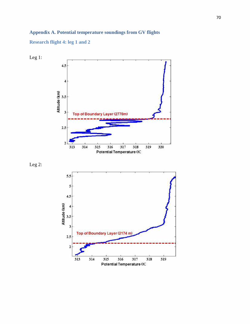
70
Appendix A. Potential temperature soundings from GV flights
Research flight 4: leg 1 and 2
Leg 1:
Leg 2:

71
Research flight 6
Research flight 8, leg 1

72
Research flight 8, leg 2
Research flight 10
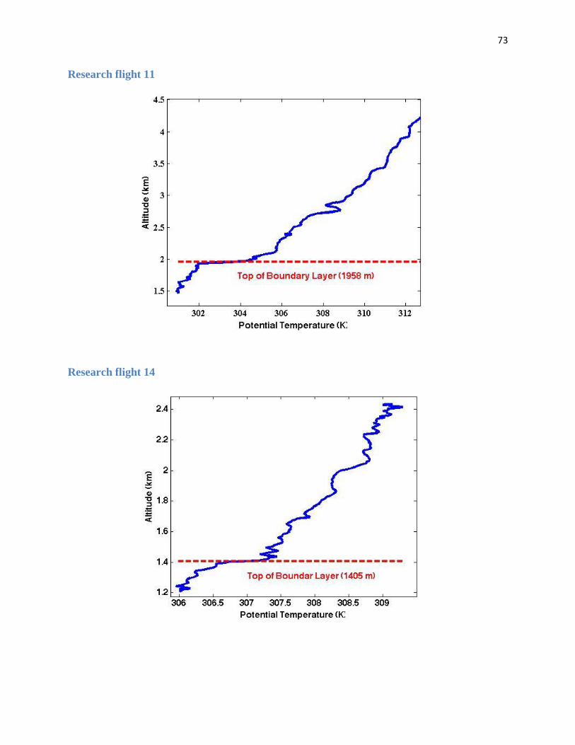
73
Research flight 11
Research flight 14

74
Research flight 17
Research flight 22, leg 1
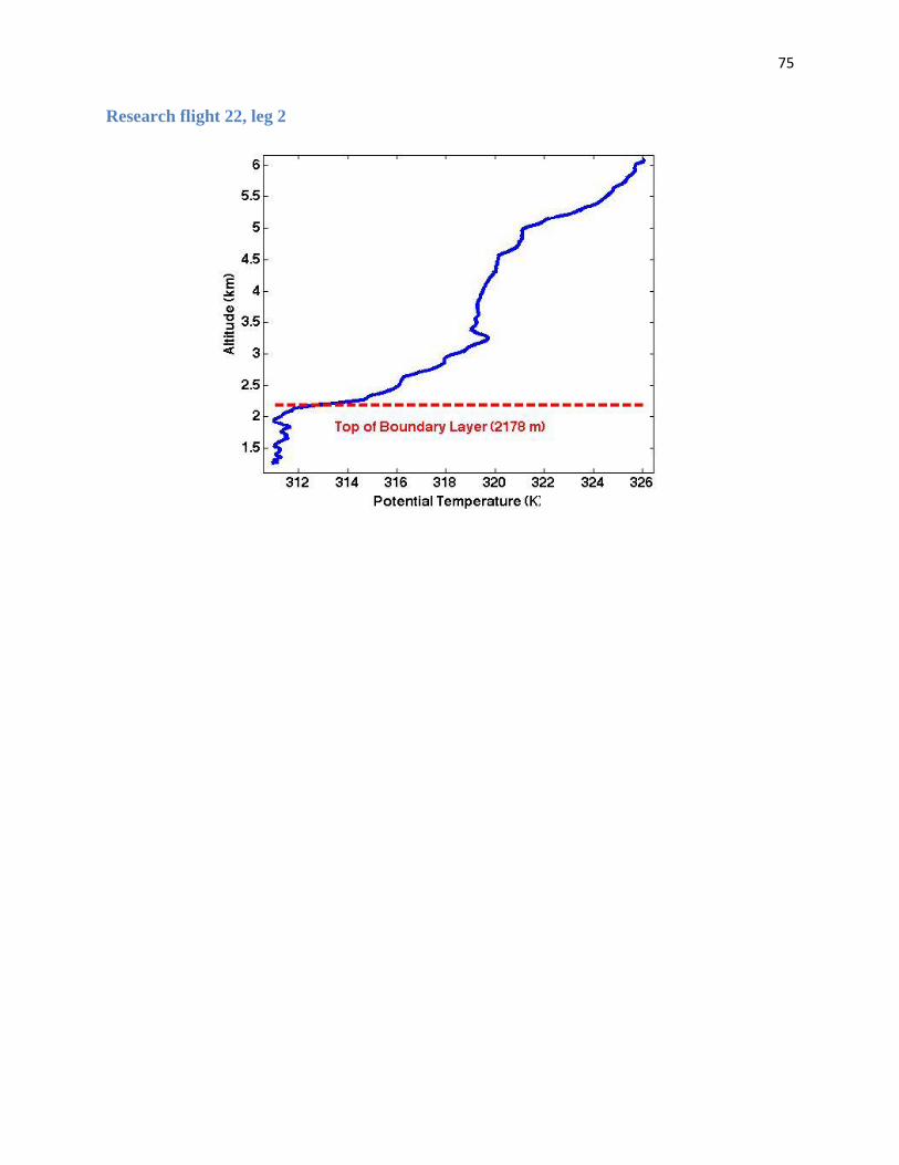
75
Research flight 22, leg 2

76
Appendix B. NEXRAD plots for flight legs with convection
Research flight 10, 22:00 UTC (1 hour prior to sampling)
Research flight 14, 20 UTC (1 hour prior to sampling, orange is approx. flight track)

77
Research flight 17, 2:00 UTC (0 hours prior to sampling)

78
Appendix C. HYSPLIT plots for flights legs within the boundary layer
Research flight 4

79
Research flight 5
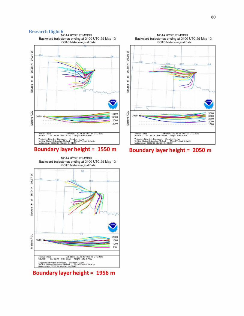
80
Research flight 6

81
Research flight 8, leg2

82
Research flight 10
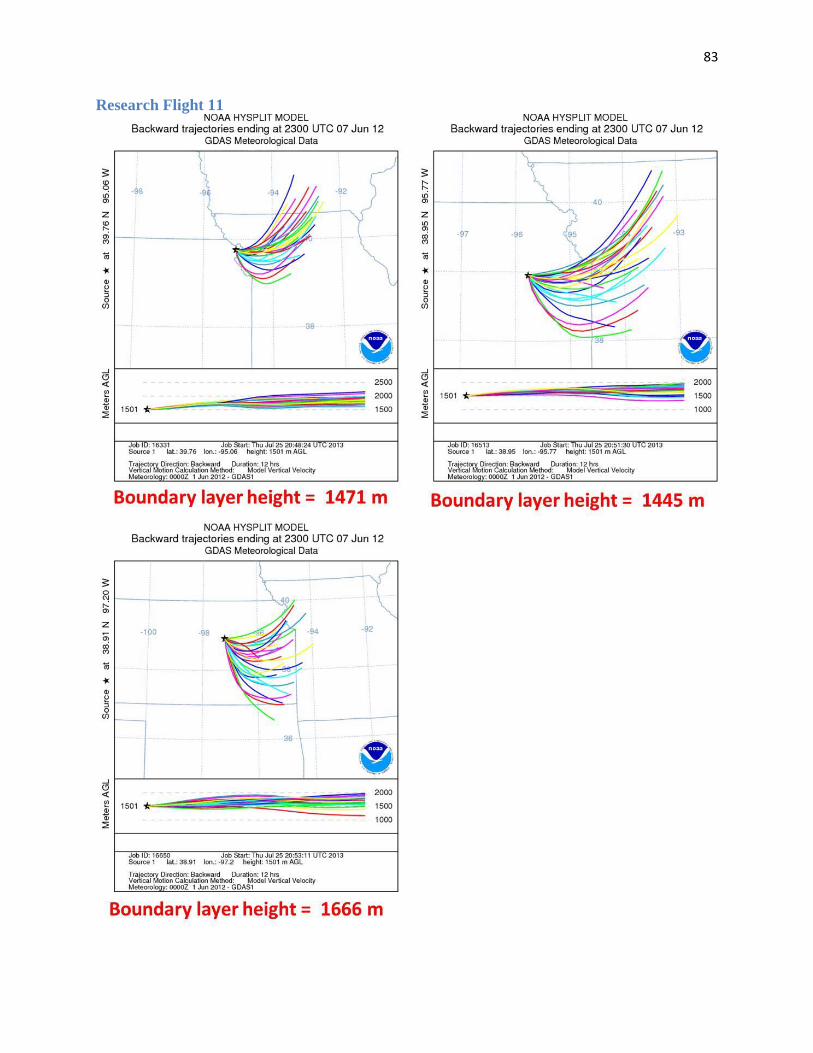
83
Research Flight 11

84
Research Flight 14

85
Research Flight 17

86
Research Flight 22, leg 1
Average GDAS mixed layer depth at starting locations: 2286m

87
Research flight 22, leg 2


