
Research ArticleESL Based Cylindrical Shell Elements with Hierarchical ShapeFunctions for Laminated Composite Shells
Jae S. Ahn,1 Seung H. Yang,2 and Kwang S. Woo2
1School of General Education, Yeungnam University, 280 Daehak-Ro, Gyeongsan, Gyeongbuk 712-749, Republic of Korea2Department of Civil Engineering, Yeungnam University, 280 Daehak-Ro, Gyeongsan, Gyeongbuk 712-749, Republic of Korea
Correspondence should be addressed to Kwang S. Woo; [email protected]
Received 7 October 2014; Accepted 7 February 2015
Academic Editor: Dane Quinn
Copyright © 2015 Jae S. Ahn et al. This is an open access article distributed under the Creative Commons Attribution License,which permits unrestricted use, distribution, and reproduction in any medium, provided the original work is properly cited.
We introduce higher-order cylindrical shell element based on ESL (equivalent single-layer) theory for the analysis of laminatedcomposite shells. The proposed elements are formulated by the dimensional reduction technique from three-dimensional solidto two-dimensional cylindrical surface with plane stress assumption. It allows the first-order shear deformation and considersanisotropic materials due to fiber orientation. The element displacement approximation is established by the integrals of Legendrepolynomials with hierarchical concept to ensure the 𝐶
0-continuity at the interface between adjacent elements as well as 𝐶1-
continuity at the interface between adjacent layers. For geometry mapping, cylindrical coordinate is adopted to implement theexact mapping of curved shell configuration with a constant curvature with respect to any direction in the plane. The verificationand characteristics of the proposed element are investigated through the analyses of three cylindrical shell problems with differentshapes, loadings, and boundary conditions.
1. Introduction
Shell structures are three-dimensional structures with anycurvature, thin in one direction and long in the other twodirections. In engineering design, they are among the mostsignificant and ubiquitous structural components. Applica-tions of them include pressure vessels, the bodies of automo-biles and airplanes, bridges, buildings, roofs, the hulls of shipsand submarines, and many other structures. Particularly,increasing application of laminated composite shell is evidentin a variety of engineering structures andmanufactured com-ponents, because of the well-recognized characteristics ofsuperior strength-to-weight, stiffness-to-weight, and cost-to-weight ratios, compared to conventional materials. While thelaminated composite materials provide the design flexibilityto achieve desirable stiffness and strength through the choiceof lamination scheme, the anisotropic constitution of lami-nated composite structures often results in stress concentra-tions near material and geometric discontinuities that canlead to damage in the form of delamination, adhesive bondseparation, and matrix cracking. Recently, these problemshave been mitigated by replacing conventionally used lami-nated composites with functionally graded materials where
the materials properties are gradually varied at microscopicscale in the thickness direction [1].
Finite element methods are versatile numerical tools tosolve differential equations related to physical phenomena.In the finite element applications for shell analysis, sometypes of shell elements are currently available. They are flatfacet element, shell theory-based element, degenerated shellelement, and solid-shell element and so forth. For the flatfacet element, it does not have any curvature.Thus, the curvedsurface is approximately explained by the combination ofseveral elements. It is very simple in formulations and hasstill been used for engineering applications. However, itcannot explain bending-stretching coupling behavior in anelement level. On the other hand, the shell theory-basedelement with curvatures can handle the bending-stretchingcoupling properly. Also, the degenerated shell element canbe used for arbitrary shapes of shell surface. Based on theflat facet element or shell theory-based element [2–6], two-dimensional shell elements have been introduced. Acknowl-edging the need of three-dimensional shell elements, severalformulations have been presented based on a degeneratedshell concept [7, 8]. Since 1990s, some solid-shell approaches,which have some benefits as compared to the degenerated
Hindawi Publishing CorporationMathematical Problems in EngineeringVolume 2015, Article ID 676181, 11 pageshttp://dx.doi.org/10.1155/2015/676181

2 Mathematical Problems in Engineering
shell element because of the simplicity of their kinematics,have been introduced by some researchers [9–11].
Meanwhile, a number of innovative approaches have beenput forward for the analysis of laminated structural systems,to extend the capabilities of laminated anisotropic compos-ites. As far as two-dimensional modeling is concerned, itis assumed that displacement components are continuouslydifferentiable through the thickness regardless of the layerboundaries. Representatives of the theories are known as clas-sical lamination theory (CLT) and first-order shear deforma-tion theory (FSDT). Both of these models [12–14] are knownas equivalent single-layer theories (ESLT) based on certainassumptions concerning the kinematics of deformation orstress across the total thickness. Although FSDT providesa sufficiently accurate description of the global laminateresponse for thin to moderately thick plates, it cannot allowdirect calculation of transverse stresses with acceptable accu-racy. So a number of higher-order theories [12, 15–17] havebeen put forward using successively third- to higher-degreepolynomials and other functions with continuous derivativesto yield more accurate interlaminar stress distributions. Thedeficiency of the theories has led to layerwisemodels inwhichthe variation of displacement functions across the thicknessis assumed for each layer separately. The layerwise models[18–21] require displacement continuity at layer interfaces.Such characterization of laminated systems can generallyexhibit a rapid change of slopes of displacement fields atlayer interfaces, often termed as the zig-zag effect. In orderto satisfy the interlaminar continuity of transverse stresses ateach layer interface, appropriate functional continuities arerequired for transverse displacements and stresses [22]. Thenumber of modal degrees of freedom in normal layerwisemodels depends on the number of layers in the laminated sys-tem. In conventional finite element analysis based mostly onLagrangian two-dimensional shape functions, the layerwisemodels can satisfy displacement continuity but not stress. It isthus true that normal layerwise models would be too expen-sive when it is intended to comply with transverse normalstress continuity. Thus, multiple model approaches [23–27]have also been attempted to reduce the overall number ofmodal degrees of freedom by optimizing computation pro-cess for maximum solution accuracy within a particular sub-region of interest only and in the process reducing the com-putational effort.
It is well-known that low-order finite element implemen-tation for shells suffers from various forms of locking when-ever purely displacement-based formulations are employed.In recent years, the issue of locking has been most promi-nently addressed through the use of low-order finite technol-ogy using mixed variational principles. The assumed strainand enhanced strain formulations are among the success-ful low-order implementations. High-order finite elementimplementations have also been advocated in recent years asa means of eliminating the locking phenomena completely.Most notably, whenever a sufficient degree of polynomial-refinement is adopted, highly reliable locking free numer-ical solutions may be obtained in a purely displacement-based setting [28]. The first 𝑝-version formulation related toshells, one of high-order approaches, was reported by Woo
NodesSide modes
Internal modes
Layer 1 Layer 2
Layer 3
𝜃
O
r
x
Constant curvature: 𝜅
Figure 1: Geometric configuration and coordinate system of theproposed element.
and Basu [29] who presented a cylindrical shell elementformulation in the cylindrical coordinates associated witha suitable transfinite mapping function to represent thecurved geometry. In this paper, we address the finite elementformulation for the laminated cylindrical shell behaviorusing the 𝑝-version approach. The approach assumes that aheterogeneous laminated shell stacked with several laminaeis treated as a shell element using hierarchic interpolationfunctions. Thus, characteristics of the proposed approachare presented in detail. Since higher-order Lagrange shapefunctions cannot be used due to excessive round-off errors,all approximate functions for displacement fields are derivedin terms of integrals of Legendre polynomials which areorthogonal in the energy norm.
2. Formulation of Cylindrical Shell Elementwith Hierarchical Shape Function
2.1. Geometry and Displacement Fields. In cylindrical coor-dinate shown in Figure 1, based on 𝐶
1
𝑟function theory with
continuity at the interface between adjacent layers, dimen-sional reduction is carried out by incorporating the first-order shear deformation for bending behavior and the planestress condition for membrane action. For geometry anddisplacement fields, the curvilinear coordinate system is con-sidered in reference to the middle surface of laminated shellskeeping a constant curvature 𝜅 with respect to any directionin the two-dimensional plane. Geometry fields on a surfacedefined by two axes are expressed by linear interpolationbetween 𝑥 and 𝜃 variables over the four vertex nodes only,as shown in Figure 1.
Also, the deformation at any point in the laminated shellis based on three displacement fields for a quadrilateralsubparametric 𝐶
0
𝑥𝜃element such as three sets of nodal
translation components (𝑢𝑖, V𝑖, and𝑤
𝑖) andmodal translation
components (𝛼𝑗, 𝛽𝑗, and 𝜒
𝑗), and two sets of nodal rotation

Mathematical Problems in Engineering 3
components (𝜌𝑖and 𝜆
𝑖) and modal rotation components (𝜑
𝑗
and 𝜓𝑗). The three displacement fields can be defined as
𝑢 (𝑥, 𝜃, 𝑟) = 𝑆𝑖𝑢𝑖+ 𝑧𝑆𝑖𝜌𝑖+ 𝐵𝑗𝛼𝑗+ 𝑟𝐵𝑗𝜙𝑗,
V (𝑥, 𝜃, 𝑟) = 𝑆𝑖V𝑖+ 𝑧𝑆𝑖𝜆𝑖+ 𝐵𝑗𝛽𝑗+ 𝑟𝐵𝑗𝜓𝑗,
𝑤 (𝑥, 𝜃, 𝑟) = 𝑆𝑖𝑤𝑖+ 𝐵𝑗𝜒𝑗,
𝑖 = 1, 2, 3, 4; 𝑗 = 5, 6, . . . , 𝑛 + 4.
(1)
In (1), indices 𝑖 and 𝑗 refer to nodal and modal contributions,and 𝑛 is the number of modal variables which is zero whendegree of polynomial approximation is one. In addition, 𝑆
𝑖
and 𝐵𝑗refer to two-dimensional shape functions in terms of
standard coordinates (𝜉, 𝜂) associated with nodal and modalvariables which are defined in next section.
2.2. Hierarchical Shape Functions. For definition of the two-dimensional shape functions, firstly one-dimensional hier-archical shape functions (𝐿
1, 𝐿2, and 𝐿
𝑗) on the basis of
standard coordinates are presented. The first two of theseshape functions in the 𝜉-direction can be defined as
𝐿1(𝜉) = 0.5 (1 − 𝜉) ,
𝐿2(𝜉) = 0.5 (1 + 𝜉) .
(2)
The shape functions corresponding to modal variables aredefined in terms of integrals of Legendre polynomials, asshown below [30]:
𝐿𝑖+1
(𝜉) = √2𝑖 − 1
2∫
𝜉
−1
1
2𝑖−1 (𝑖 − 1)!
𝑑𝑖−1
𝑑𝑤𝑖−1(𝑤2− 1)𝑖−1
𝑑𝑤
𝑖 = 2, 3, 4, . . . .
(3)
For 𝜂- and 𝜁-directions, analogous expressions areobtained by replacing 𝜉 by 𝜂 and 𝜁, respectively, in (2) and (3).One-dimensional shape functions are used to construct two-dimensional shape functions, 𝑆
𝑖and 𝐵
𝑗, in the 𝜉, 𝜂-plane. In
other words, two-dimensional shape functions at four cornernodes can be obtained by a product of two one-dimensionalnodal functions in the following:
𝑆1(𝜉, 𝜂) = 𝐿
1(𝜉)𝑁1(𝜂) ,
𝑆2(𝜉, 𝜂) = 𝐿
2(𝜉)𝑁1(𝜂) ,
𝑆3(𝜉, 𝜂) = 𝐿
2 (𝜉)𝑁2 (𝜂) ,
𝑆4(𝜉, 𝜂) = 𝐿
1(𝜉)𝑁2(𝜂) .
(4)
Next, the modal variables of two-dimensional shape func-tions of laminated systems are classified into two groups suchas “side modes” and “internal modes” as shown in Figure 1.
The number of modal variables 𝑓 is dependent on the degreeof polynomial (𝑝-level), as shown in the following:
𝑓side
(𝑝) = 4 (𝑝 − 1) ,
𝑓internal
(𝑝) =
{{
{{
{
0 in 𝑝 ≤ 3
(𝑝 − 2) (𝑝 − 3)
2in 𝑝 ≥ 4.
(5)
The shape functions for side modal variables for any 𝑝-levelare shown in (6).The superscripts in (6) refer to side numbers:
𝐵1
𝑖(𝜉, 𝜂) = 𝐿
1(𝜂) 𝐿𝑖+1
(𝜉) ,
𝐵2
𝑖(𝜉, 𝜂) = 𝐿
2(𝜉) 𝐿𝑖+1
(𝜂) ,
𝐵3
𝑖(𝜉, 𝜂) = 𝐿
2(𝜂) 𝐿𝑖+1
(𝜉) ,
𝐵4
𝑖(𝜉, 𝜂) = 𝐿
1 (𝜉) 𝐿 𝑖+1 (𝜂) ,
with 2 ≤ 𝑖 ≤ 𝑝.
(6)
The shape functions for internal modal variables are obtainedby
𝐵internal
(𝜉, 𝜂) = 𝐿𝑖(𝜉) 𝐿𝑗(𝜂)
𝑖 + 𝑗 = 𝑝 + 2 𝑖, 𝑗 = 3, 4, . . . .
(7)
2.3. Strain and Stress Relations. The three strain componentscan be denoted by membrane (𝑚), bending (𝑏), and shear (𝑡)strain, respectively:
{{{{{{{{
{{{{{{{{
{
𝜀𝑥
𝜀𝜃
𝛾𝑥𝜃
𝛾𝑥𝑟
𝛾𝜃𝑟
}}}}}}}}
}}}}}}}}
}
=
{{{{{{{{
{{{{{{{{
{
𝜀𝑚
𝑥
𝜀𝑚
𝜃
𝛾𝑚
𝑥𝜃
𝛾𝑡
𝑥𝑟
𝛾𝑡
𝜃𝑟
}}}}}}}}
}}}}}}}}
}
+ 𝑟
{{{{{{{{{
{{{{{{{{{
{
𝜀𝑏
𝑥
𝜀𝑏
𝜃
𝛾𝑏
𝑥𝜃
0
0
}}}}}}}}}
}}}}}}}}}
}
, (8)
where
[[
[
𝜀𝑚
𝑥
𝜀𝑚
𝜃
𝛾𝑚
𝑥𝜃
]]
]
=
[[[[[[[[
[
𝜕𝑆𝑖
𝜕𝜉0 0
𝜕𝐵𝑗
𝜕𝜉0 0
0𝜅𝜕𝑆𝑖
𝜕𝜂𝜅𝑆𝑖
0𝜅𝜕𝐵𝑗
𝜕𝜂𝜅𝐵𝑗
𝜅𝜕𝑆𝑖
𝜕𝜂
𝜕𝑆𝑖
𝜕𝜉0
𝜅𝜕𝐵𝑗
𝜕𝜂
𝜕𝐵𝑗
𝜕𝜉0
]]]]]]]]
]
[[[[[[[[[[[
[
𝑢𝑖
V𝑖
𝑤𝑖
𝛼𝑗
𝛽𝑗
𝜒𝑗
]]]]]]]]]]]
]
,
4 Mathematical Problems in Engineering
[[[
[
𝜀𝑏
𝑥
𝜀𝑏
𝜃
𝛾𝑏
𝑥𝜃
]]]
]
=
[[[[[[[[
[
0𝜕𝑆𝑖
𝜕𝜉0
𝜕𝐵𝑗
𝜕𝜉
𝜅𝜕𝑆𝑖
𝜕𝜂0
𝜅𝜕𝐵𝑗
𝜕𝜂0
𝜕𝑆𝑖
𝜕𝜉
𝜅𝜕𝑆𝑖
𝜕𝜂
𝜕𝐵𝑗
𝜕𝜉
𝜅𝜕𝐵𝑗
𝜕𝜂
]]]]]]]]
]
[[[[[
[
𝜆𝑖
𝜌𝑖
𝜓𝑗
𝜙𝑗
]]]]]
]
,
[𝛾𝑡
𝑥𝑟
𝛾𝑡
𝜃𝑟
] =
[[[[
[
0𝜕𝑆𝑖
𝜕𝜉𝑆𝑖
0 0𝜕𝐵𝑗
𝜕𝜉𝐵𝑖
0
−𝜅𝑆𝑖
𝜅𝜕𝑆𝑖
𝜕𝜂0 𝑆𝑖−𝜅𝐵𝑗
𝜅𝜕𝐵𝑗
𝜕𝜂0 𝐵𝑗
]]]]
]
[[[[[[[[[[[[[[[[[
[
V𝑖
𝑤𝑖
𝜆𝑖
𝜌𝑖
𝛽𝑗
𝜒𝑗
𝜓𝑗
𝜙𝑗
]]]]]]]]]]]]]]]]]
]
.
(9)
The constitutive relationship for the laminate with respect tothe reference surface can then be expressed as
{��} = [𝐸]8×8 {𝜀} , (10)
where [𝐸]8×8
is the constitutive matrix including membrane,bending, and transverse shear force resultants to referencesurface strains and curvatures. The stress resultant vector {��}will be of the form
{��} =
{{
{{
{
{𝑁}3×1
{𝑀}3×1
{𝑄}2×1
}}
}}
}
. (11)
Here letters 𝑁, 𝑀, and 𝑄 refer to resultants of membranestresses, bending stresses, and transverse shear stresses. Basedon (10) and (11), the stress resultants can be defined by
{𝑁}3×1
=
𝑛
∑
𝑙=1
∫
𝑟top𝑙
𝑟bottom𝑙
[𝐷𝑖𝑗]𝑙
5×5
{{{
{{{
{
𝜀𝑚
𝑥+ 𝑟𝜀𝑏
𝑥
𝜀𝑚
𝜃+ 𝑟𝜀𝑏
𝜃
𝛾𝑚
𝑥𝜃+ 𝑟𝛾𝑏
𝑥𝜃
}}}
}}}
}
𝑑𝑟;
𝑖, 𝑗 = 1, 2, 3,
{𝑀}3×1
=
𝑛
∑
𝑙=1
∫
𝑟top𝑙
𝑟bottom𝑙
[𝐷𝑖𝑗]𝑙
5×5
{{{
{{{
{
𝑟𝜀𝑚
𝑥+ 𝑟2𝜀𝑏
𝑥
𝑟𝜀𝑚
𝜃+ 𝑟2𝜀𝑏
𝜃
𝑟𝛾𝑚
𝑥𝜃+ 𝑟2𝛾𝑏
𝑥𝜃
}}}
}}}
}
𝑑𝑟;
𝑖, 𝑗 = 1, 2, 3,
{𝑄}2×1
= 𝐾
𝑛
∑
𝑙=1
∫
𝑟top𝑙
𝑟bottom𝑙
[𝐷𝑖𝑗]𝑙
5×5{𝛾𝑡
𝑥𝑟
𝛾𝑡
𝜃𝑟
}𝑑𝑟 𝑖, 𝑗 = 4, 5,
(12)
where elasticity matrix [𝐷] represents anisotropy with threemutually orthogonal planes of symmetry. The elasticity
matrix includes shear correction factors 𝐾 in order to allowfor the error resulting from the use of transverse shearstrain energy on an average basis which depends on laminaproperties and the lamination scheme. 𝑟bottom
𝑙and 𝑟
top𝑙
aredistances from the reference surface to bottom and topsurfaces of lamina. ℓ and 𝑛 are the number of laminasmakingup the thickness of laminated shells.
2.4. Finite Element Formulation. The displacement fieldsdefined by (1) can be represented in the following generalform:
��𝑖= [��]
𝑖
1×𝑛{��}𝑖
𝑛×1𝑖 = 1, 2, and 3, (13)
where the matrix [��] indicates hierarchical shape functionsfor nodal and modal variables �� with total number ofvariables denoted by 𝑛. The finite element equation for eachmodel can be expressed by using the principle of virtual work
𝛿𝑈𝜀− 𝛿𝑊 = 0. (14)
The internal virtual strain is
𝛿𝑈𝜀= ∫𝑉
𝛿 {𝜀}𝑇{��} 𝑑𝑉 (15)
with {𝜀} and {��} being the strain and stress tensors used in (8).If the virtual displacements are defined as
𝛿𝑢 = [��] 𝛿 {��} (16)
the virtual strains can be written as
𝛿 {𝜀} = [𝐵] 𝛿 {��} , (17)
where [𝐵] is the strain-displacement matrix. The externalvirtual work takes the following form:
𝛿𝑊 = 𝛿 {��}𝑇{𝐹}𝑎+ ∫𝑆
𝛿 {��}𝑇{𝐹𝑏} 𝑑𝑆 + ∫
𝐴
𝛿 {��}𝑇{𝐹}𝑐𝑑𝐴.
(18)
Here the superscripts 𝑎, 𝑏, 𝑐, and 𝑑 refer to nodal andmodal forces, side forces, surface forces, and body forces,respectively. Based on these definitions, the virtual workequation shown in (14) can be rewritten as
∫𝑉
𝛿 [𝐵]𝑇
[𝐷] [𝐵] 𝑑𝑉�� = 𝛿 {��}𝑇{𝐹}𝑎+ ∫𝑆
𝛿 {��}𝑇{𝐹}𝑏𝑑𝑆
+ ∫𝐴
𝛿 {��}𝑇{𝐹}𝑐𝑑𝐴
+ ∫𝑉
𝛿 {��}𝑇{𝐹}𝑑𝑑𝑉.
(19)
Here constitutive matrix [𝐷] on the basis of the local coordi-nate system is obtained by the following transformation frommaterial axes to local axes using the transformation matrix[𝑋]:
[𝐷] = [𝑋]𝑇[𝐷] [𝑋] . (20)

Mathematical Problems in Engineering 5
r r
x
t
s
p pR
R
𝜃
Figure 2: Orthotropic clamped cylindrical shells with internalpressure.
3. Numerical Examples
The performance of proposed cylindrical shell element withhierarchical shape function is investigated and comparedwith results obtained by some conventional finite elementmethods [31] via the following numerical examples in whichall units of parameters are expressed by nondimensionalvalues. Three types of conventional finite elements are con-sidered such as 4-node element (4N) with linear Lagrangianpolynomials, 8-node element (8N) often called serendipityelement, and 9-node element (9N)with quadratic Lagrangianpolynomials. Also all conventional finite elements adopt dif-ferent integration techniques, separately, like full (F), reduced(R), and selective reduced (S) integration. For present analysisand conventional finite elements, identical linear mappingbased on cylindrical coordinate is implemented. For conver-gence, present analysis is implemented based on dominantly𝑝-refinement, occasionally ℎ-refinement, while conventionalfinite elements choose only ℎ-refinement in which all calcu-lated values have four or five significant digits.
3.1. Orthotropic Cylindrical Shells with Internal Pressure.Firstly, displacements of cylindrical shells with one layer (0∘)and two layers (0∘/90∘ from inner surface) subject to internalpressure 𝑝 (=6410/𝜋) as shown in Figure 2 are estimated.In the problem with two layers, thickness of two layers isidentical. Length 𝑠 of the shell is 20, the radius 𝑅 is 20, andthe total thickness 𝑡 is 1. Each layer is a unidirectional fiberreinforced composite with the following material constants:
𝐸1= 7.5 × 10
6; 𝐸
2= 2 × 10
6; 𝐺
12= 1.25 × 10
6;
𝐺13
= 𝐺23
= 0.625 × 10⁶; ]
12= 0.25,
(21)
where subscript 1 signifies the direction parallel to fibers and 2and 3 the transverse direction. In these problems, the number1 means 𝑥 direction, the number 2 is 𝜃 direction, and thenumber 3 refers to 𝑟 direction, respectively. Also, clampedboundary conditions are specified at both ends of the shelland only octant of the shell is considered to take advantage ofthree-way symmetry.
Table 1 gives the maximum displacement results in thecylindrical shell with one layer. All converged values arealmost identical except those of 4-node element case. Presentanalysis using only one element has the converged value
Computational region
p
s
tx r
R
O
𝜃
𝛼
Figure 3: Clamped cylindrical shell panels with uniform load.
from 𝑝-level = 4, while 8-node and 9-node elements require8×8mesh. Table 2 shows the maximum displacement resultswith two layers. It is noted that similar characteristics areobtained. Also, Tables 1 and 2 show the converged valuesshaded according to analysis types.
3.2. Isotropic Cylindrical Shell Panels with Uniformly Dis-tributed Load. Next, an isotropic (𝐸 = 0.45×10
6 and ] = 0.3)cylindrical shell panel is considered. Figure 3 shows geometryshape of the panel and loading condition (𝑝 = 0.04) of whichspecific values are as follows:
𝛼 = 0.2; 𝑅 = 100; 𝑠 = 20; 𝑡 = 0.125. (22)
A quarter of panel is considered as a computational regionshown in Figure 3 by specifying symmetry conditions withrespect to 𝑥 and 𝜃 axes. At 𝑥 = 𝑠, clamped conditions areapplied and free boundary is defined at 𝜃 = 0. Figures 4(a)and 4(b) show the variation of maximum vertical deflectionwith respect to the number of degrees of freedom (NDF)obtained by all elements considered. The converged valuesare all identical except 4NF which requires more fine meshrefinement to obtain a converged value. For the conventionalfinite elements, it is seen that convergence rates with fullintegration are slower than those elements with reduced orselective reduced integration because of shear locking prob-lem. Present analysis with full integration gives much fasterconvergence than the other elements to keep same convergedvalue. Table 3 shows specific values with respect to analysistypes. For present analysis, the maximum displacement isconverged from 𝑝-level = 6 or 7 with 2×2mesh. Also, for theconventional finite elements with 8N and 9N, there is littledifference according to integration techniques. It is noticedthat the shear behavior is not significant as the thickness ratiobecomes very thin (𝑆/𝑡 = 160) and thus the effect of selectivereduced integration is worthless.
3.3. Pinched Cylinder with Rigid End Diaphragms. This isanother well-known benchmark problem. Figure 5 shows

6 Mathematical Problems in Engineering
Table 1: Maximum displacements of the cylindrical shell with one layer.
Analysis types 1 × 1 2 × 2 4 × 4 8 × 8 16 × 16Present analysis
𝑝-level = 3 0.3798 — — — —𝑝-level = 4 0.3746 — — — —𝑝-level = 5 0.3748 — — — —𝑝-level = 6 0.3748 — — — —𝑝-level = 7 0.3748 — — — —𝑝-level = 8 0.3748 — — — —𝑝-level = 9 0.3748 — — — —𝑝-level = 10 0.3748 — — — —
4NF 0.1478 0.2816 0.3484 0.3681 0.3731R 0.1574 0.4072 0.3844 0.3772 0.3754S 0.1574 0.4072 0.3844 0.3772 0.3754
8NF 0.3220 0.3729 0.3747 0.3748 0.3748R 0.4179 0.3770 0.3750 0.3748 0.3748S 0.4179 0.3770 0.3750 0.3748 0.3748
9NF 0.3129 0.3728 0.3747 0.3748 0.3748R 0.4179 0.3770 0.3749 0.3748 0.3748S 0.4179 0.3770 0.3749 0.3748 0.3748
Table 2: Maximum deflections of the cylindrical laminate shell with two layers.
Analysis types 1 × 1 2 × 2 4 × 4 8 × 8 16 × 16Present analysis
𝑝-level = 3 0.1860 — — — —𝑝-level = 4 0.1782 — — — —𝑝-level = 5 0.1795 — — — —𝑝-level = 6 0.1794 — — — —𝑝-level = 7 0.1794𝑝-level = 8 0.1794 — — — —𝑝-level = 9 0.1794 — — — —𝑝-level = 10 0.1794
4NF 0.1105 0.1705 0.1811 0.1804 0.1797R 0.1240 0.2290 0.1882 0.1814 0.1799S 0.1240 0.2290 0.1882 0.1814 0.1799
8NF 0.1829 0.1830 0.1797 0.1795 0.1794R 0.2174 0.1796 0.1794 0.1794 —S 0.2174 0.1796 0.1794 0.1794 —
9NF 0.1829 0.1830 0.1797 0.1795 0.1794R 0.2174 0.1796 0.1794 0.1794 —S 0.2174 0.1796 0.1794 0.1794 —

Mathematical Problems in Engineering 7
Table 3: Maximum vertical deflection (−𝑤 × 102) at the center of cylindrical panels.
Analysis types 1 × 1 2 × 2 4 × 4 8 × 8 16 × 16Present analysis
𝑝-level =3 0.4903 1.0048𝑝-level = 4 0.5410 1.1534𝑝-level = 5 1.2248 1.1403𝑝-level = 6 1.2525 1.1358𝑝-level = 7 1.1175 1.1349𝑝-level = 8 1.1455 1.1349𝑝-level = 9 1.1320 1.1349𝑝-level = 10 1.1359 1.1349
4NF 0.0082 0.0309 0.1075 0.3378 0.7456R 0.0111 1.7227 1.2376 1.1577 1.1404S 0.0110 1.7154 1.2400 1.1584 1.1406
8NF 0.0461 0.7435 1.1745 1.1428 1.1362R 1.6496 0.9573 1.1375 1.1350 1.1349S 1.6399 0.9563 1.1374 1.1350 1.1349
9NF 0.0463 1.3469 1.1721 1.1427 1.1362R 1.6668 1.1444 1.1352 1.1349 1.1349S 1.6532 1.1434 1.1352 1.1349 1.1349
00.20.40.60.8
11.21.41.61.8
2
Vert
ical
defl
ectio
ns (−
w×10
2)
Present4NF8NF9NF
0 200 400 600 800 1000NDF
(a) Convergence characteristics by full integration
00.20.40.60.8
11.21.41.61.8
2
0 100 200 300 400 500NDF
Present4NR, 4NS8NR, 8NS9NR, 9NS
Vert
ical
defl
ectio
ns (−
w×10
2)
(b) Convergence characteristics by reduced and selective reduced inte-gration
Figure 4: Convergence of maximum displacement with respect to NDF.
a cylinder with rigid end diaphragms subjected to two pointloads (𝑃 = 1). Geometry data in Figure 5 is given by
𝑆 = 600; 𝑅 = 300; 𝑡 = 3.0. (23)
For material conditions, isotropic material (𝐸 = 3 × 10⁶ and
] = 0.3) is firstly considered. For a numerical analysis, only
octant of the entire shell is modelled taking advantage ofthree-way symmetry as shown in Figure 5.
This problem is known as one of bench mark problemswith bending-dominant behavior in the thin limit. Thustransverse shear locking and membrane locking occur as theshell is getting thinner. Table 4 shows the maximum radialdisplacement at the point of load application. The analytical

8 Mathematical Problems in Engineering
Table 4: Maximum radial deflection (−𝑤 × 105) at 𝑅/𝑡 = 100.
Analysis types 1 × 1 2 × 2 4 × 4 8 × 8 16 × 16 20 × 20Present analysis
𝑝-level = 3 0.0674 0.3540 1.2273 1.7090 1.8172 1.8293𝑝-level = 4 0.1489 0.8821 1.5689 1.7825 1.8350 1.8404𝑝-level = 5 0.3503 1.3250 1.6937 1.8147 1.8419 1.8452𝑝-level = 6 0.7655 1.5009 1.7542 1.8289 1.8458 1.8481𝑝-level = 7 1.1906 1.6180 1.7937 1.8376 1.8485 1.8503𝑝-level = 8 1.3670 1.7037 1.8162 1.8426 1.8504 1.8520𝑝-level = 9 1.4789 1.7560 1.8284 1.8457 1.8519 1.8533𝑝-level = 10 1.5897 1.7883 1.8356 1.8479 1.8532 1.8545
4NF 0.0098 0.0254 0.0608 0.1282 0.2785 0.3603R 0.0207 0.3263 1.9281 1.8453 1.8600 1.8632S 0.0213 0.6723 1.3929 1.6093 1.7762 1.8056
8NF 0.0369 0.0864 0.3891 1.1772 1.6691 1.7378R 0.1477 1.0976 1.6444 1.7951 1.8307 1.8365S 0.1263 0.8565 1.5541 1.7799 1.8282 1.8350
9NF 0.0414 0.0925 0.4184 1.2238 1.6845 1.7476R 0.1886 1.7458 1.8451 1.8596 1.8677 1.8702S 0.1657 1.2428 1.7046 1.8359 1.8633 1.8675
Rigid diaphragm
Rigid diaphragm
Computational region
P
P
Rt
x
r
s
B
A 𝜃
Figure 5: Pinched cylinder with rigid diaphragms.
solution is −1.8248 × 10⁻⁵ from [32] which used the shell
theory without transverse shear deformation. Cho and Roh[33] proposed −1.8541 × 10
−5 by including the transverseshear deformation. All results of present analysis and theconventional finite elements approach to the reference value(−1.8541 × 10
−5) as the number of elements is increased.
For present analysis, it is difficult to obtain the convergedvalue when only 𝑝-refinement is implemented. Also, it isseen in Table 4 that the converged solution of present analysisrequires ℎ- and 𝑝-refinement simultaneously. For 𝑝-level ≥ 7
in the 8×8mesh, the relative error ofmaximumdisplacementis less than 1.0% as compared with the reference value.
Next, the cylindrical laminated shell with two layers isanalyzed. The thickness of two layers is identical and totalthickness 𝑡 of the cylinder is fixed as 3.0. Each layer consistsof a unidirectional fiber reinforced composite with followingmaterial constants:
𝐸𝐿= 25𝐸
𝑇; 𝐺
𝐿𝑇= 0.5𝐸
𝑇; 𝐺
𝑇𝑇= 0.2𝐸
𝑇;
]𝐿𝑇
= ]𝑇𝑇
= 0.25,
(24)
where subscript 𝐿 signifies the direction parallel to the fibers,𝑇 is the transverse direction, and ]
𝐿𝑇is the Poisson’s ratio for
strain in the𝑇 direction under uniaxial normal stress in the 𝐿direction. 𝐸
𝑇is an elastic modulus in the transverse direction
and 𝐺 is an elastic shear modulus. The normalized quantitiesof interest are defined as follows:
𝑤 =−10𝑤A𝐸1𝑡
3
𝑃𝑅2; 𝑢 =
−10𝑢B𝐸1𝑡2
𝑃𝑅, (25)
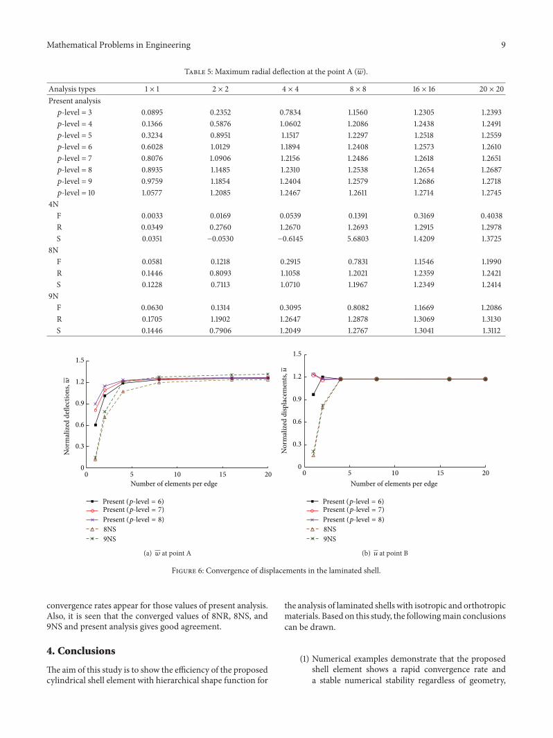
where 𝑤A means the deflection at the point A and 𝑢Brefers to the displacement in the 𝑥 direction at the point B.Figures 6(a) and 6(b) show the convergence characteristicsof 𝑤 and 𝑢 displacements, respectively. It is seen that theconverged values of all elements are almost same. Table 5contains the normalized deflections at the point A. Thevalues of present analysis are close to 1.27 by ℎ𝑝-refinement,while the values of 8NR/S and 9NR/S reach 1.24 and 1.31.The difference between present solutions and ℎ-refinementanalyses is within 2∼3%. Table 6 shows displacements in 𝑥
direction at point B. Unlike deflection values at point A, high
Mathematical Problems in Engineering 9
Table 5: Maximum radial deflection at the point A (𝑤).
Analysis types 1 × 1 2 × 2 4 × 4 8 × 8 16 × 16 20 × 20Present analysis
𝑝-level = 3 0.0895 0.2352 0.7834 1.1560 1.2305 1.2393𝑝-level = 4 0.1366 0.5876 1.0602 1.2086 1.2438 1.2491𝑝-level = 5 0.3234 0.8951 1.1517 1.2297 1.2518 1.2559𝑝-level = 6 0.6028 1.0129 1.1894 1.2408 1.2573 1.2610𝑝-level = 7 0.8076 1.0906 1.2156 1.2486 1.2618 1.2651𝑝-level = 8 0.8935 1.1485 1.2310 1.2538 1.2654 1.2687𝑝-level = 9 0.9759 1.1854 1.2404 1.2579 1.2686 1.2718𝑝-level = 10 1.0577 1.2085 1.2467 1.2611 1.2714 1.2745
4NF 0.0033 0.0169 0.0539 0.1391 0.3169 0.4038R 0.0349 0.2760 1.2670 1.2693 1.2915 1.2978S 0.0351 −0.0530 −0.6145 5.6803 1.4209 1.3725
8NF 0.0581 0.1218 0.2915 0.7831 1.1546 1.1990R 0.1446 0.8093 1.1058 1.2021 1.2359 1.2421S 0.1228 0.7113 1.0710 1.1967 1.2349 1.2414
9NF 0.0630 0.1314 0.3095 0.8082 1.1669 1.2086R 0.1705 1.1902 1.2647 1.2878 1.3069 1.3130S 0.1446 0.7906 1.2049 1.2767 1.3041 1.3112
0
0.3
0.6
0.9
1.2
1.5
0 5 10 15 20Number of elements per edge
8NS9NS
Present (p-level = 6)Present (p-level = 7)Present (p-level = 8)
Nor
mal
ized
defl
ectio
ns,w
(a) 𝑤 at point A
0
0.3
0.6
0.9
1.2
1.5
0 5 10 15 20
Nor
mal
ized
disp
lace
men
ts,u
Number of elements per edge
8NS9NS
Present (p-level = 6)Present (p-level = 7)Present (p-level = 8)
(b) 𝑢 at point B
Figure 6: Convergence of displacements in the laminated shell.
convergence rates appear for those values of present analysis.Also, it is seen that the converged values of 8NR, 8NS, and9NS and present analysis gives good agreement.
4. Conclusions
The aim of this study is to show the efficiency of the proposedcylindrical shell element with hierarchical shape function for
the analysis of laminated shells with isotropic and orthotropicmaterials. Based on this study, the followingmain conclusionscan be drawn.
(1) Numerical examples demonstrate that the proposedshell element shows a rapid convergence rate anda stable numerical stability regardless of geometry,

10 Mathematical Problems in Engineering
Table 6: Displacement in 𝑥 direction at the point B (𝑢).
Analysis types 1 × 1 2 × 2 4 × 4 8 × 8 16 × 16 20 × 20Present analysis
𝑝-level = 3 0.1627 0.3403 0.9709 — — —𝑝-level = 4 0.2256 0.9344 1.1661 — — —𝑝-level = 5 0.5338 1.2390 1.1712 — — —𝑝-level = 6 0.9668 1.1987 1.1725 — — —𝑝-level = 7 1.2283 1.1667 1.1714 — — —𝑝-level = 8 1.2321 1.1742 1.1711 — — —𝑝-level = 9 1.1539 1.1694 1.1711 — — —𝑝-level = 10 1.1458 1.1703 1.1711 — — —
4NF −0.0020 0.0040 0.0387 0.1132 0.2539 0.3253R −0.0006 0.3669 1.2780 1.1706 1.1692 1.1697S −0.0714 −0.1049 0.0660 0.7326 1.2604 1.2261
8NF 0.0937 0.1678 0.3530 0.8797 1.1372 1.1558R 0.2010 1.0642 1.1594 1.1709 1.1711 1.1711S 0.1522 0.7955 1.1710 1.1704 1.1710 1.1711
9NF 0.1022 0.1628 0.3519 0.8797 1.1372 1.1558R 0.2082 0.9531 1.1692 1.1692 1.1705 1.1707S 0.2039 0.8190 1.1716 1.1707 1.1710 1.1711
loading, and boundary condition as compared withthe conventional finite element approaches.
(2) The proposed element can endure very thin thicknessratio without any special numerical integration tech-nique. It may be concluded that membrane and shearlocking are considerably free over 𝑝-level = 4 or 5.
(3) From these results, it is necessary to develop thehierarchical shell elementswith arbitrary geometry byapplying the advanced mapping technique.
Finally, although this study deals with classical shell prob-lems, it is important to note that the proposed shell elementsbased on high-order approaches can be extended to applica-tions of various shell problems with cutout and functionallygraded materials which many researchers have recently beeninterested in.
Conflict of Interests
The authors declare that there is no conflict of interestsregarding the publication of the paper.
Acknowledgment
Thisworkwas supported byNational Research Foundation ofKorea (NRF) grant funded by the Korea government (MEST)(NRF-2013R1A1A2057756).
References
[1] K. Swaminathan, D. T. Naveenkumar, A. M. Zenkour, andE. Carrera, “Stress, vibration and buckling analyses of FGMplates—a state-of-the-art review,”Composite Structures, vol. 120,pp. 10–31, 2015.
[2] J. A. Stricklin, J. E. Martinez, J. R. Tillerson, J. H. Hong, and W.E. Haisler, “Nonlinear dynamic analysis of shells of revolutionbymatrix displacementmethod,”AIAA Journal, vol. 9, no. 4, pp.629–636, 1971.
[3] H. U. Akay, “Dynamic large deflection analysis of plates usingmixed finite elements,” Computers & Structures, vol. 11, no. 1-2,pp. 1–11, 1980.
[4] J.N. Reddy, “Dynamic (transient) analysis of layered anisotropiccomposite-material plates,” International Journal for NumericalMethods in Engineering, vol. 19, no. 2, pp. 237–255, 1983.
[5] Y. C. Wu, T. Y. Yang, and S. Saigal, “Free and forced nonlineardynamics of composite shell structures,” Journal of CompositeMaterials, vol. 21, no. 10, pp. 898–909, 1987.
[6] T. Park, K. Kim, and S. Han, “Linear static and dynamic analysisof laminated composite plates and shells using a 4-node quasi-conforming shell element,” Composites Part B: Engineering, vol.37, no. 2-3, pp. 237–248, 2006.
[7] S. Ahmad, B. M. Irons, and O. C. Zienkiewicz, “Analysis ofthick and thin shell structures by curved finite elements,”International Journal for Numerical Methods in Engineering, vol.2, no. 3, pp. 419–451, 1970.
[8] T. J. R. Hughes andW. K. Liu, “Nonlinear finite element analysisof shells: part I. three-dimensional shells,”ComputerMethods inApplied Mechanics and Engineering, vol. 26, no. 3, pp. 331–362,1981.

Mathematical Problems in Engineering 11
[9] K. Y. Sze, S. Yi, and M. H. Tay, “An explicit hybrid stabilizedeighteen-node solid element for thin shell analysis,” Interna-tional Journal for Numerical Methods in Engineering, vol. 40, no.10, pp. 1839–1856, 1997.
[10] L. Vu-Quoc and X. G. Tan, “Optimal solid shells for non-linearanalyses ofmultilayer composites. I. Statics,”ComputerMethodsin Applied Mechanics and Engineering, vol. 192, no. 9-10, pp.975–1016, 2003.
[11] K. Rah, W. van Paepegem, A. M. Habraken, and J. Degrieck, “Apartial hybrid stress solid-shell element for the analysis of lami-nated composites,”ComputerMethods inAppliedMechanics andEngineering, vol. 200, no. 49-52, pp. 3526–3539, 2011.
[12] J. N. Reddy, “Simple higher-order theory for laminated com-posite plates,” Transactions of the ASME Journal of AppliedMechanics, vol. 51, no. 4, pp. 745–752, 1984.
[13] K. Wisniewski and B. A. Schrefler, “Hierarchical multi-layeredelement of assembled timoshenko beams,” Computers & Struc-tures, vol. 48, no. 2, pp. 255–261, 1993.
[14] A. Idlbi, M. Karama, and M. Touratier, “Comparison of variouslaminated plate theories,”Composite Structures, vol. 37, no. 2, pp.173–184, 1997.
[15] Y. W. Kwon and J. E. Akin, “Analysis of layered compositeplates using a high-order deformation theory,” Computers andStructures, vol. 27, no. 5, pp. 619–623, 1987.
[16] B. N. Pandya and T. Kant, “A refined higher-order generallyorthotropic C0 plate bending element,”Computers & Structures,vol. 28, no. 2, pp. 119–133, 1988.
[17] B. N. Pandya and T. Kant, “Flexural analysis of laminated com-posites using refined higher-order C∘ plate bending elements,”Computer Methods in Applied Mechanics and Engineering, vol.66, no. 2, pp. 173–198, 1988.
[18] J. N. Reddy and M. Savoia, “Layer-wise shell theory for post-buckling of laminated circular cylindrical shells,”AIAA Journal,vol. 30, no. 8, pp. 2148–2154, 1992.
[19] N. U. Ahmed and P. K. Basu, “Higher-order finite elementmodelling of laminated composite plates,” International Journalfor Numerical Methods in Engineering, vol. 37, no. 1, pp. 123–139,1994.
[20] Y. B. Cho and R. C. Averill, “First-order zig-zag sublaminateplate theory and finite element model for laminated compositeand sandwich panels,” Composite Structures, vol. 50, no. 1, pp.1–15, 2000.
[21] P. F. Pai and A. N. Palazotto, “A higher-order sandwich platetheory accounting for 3-D stresses,” International Journal ofSolids and Structures, vol. 38, no. 30-31, pp. 5045–5062, 2001.
[22] E. Carrera, “Historical review of Zig-Zag theories for multilay-ered plates and shells,” Applied Mechanics Reviews, vol. 56, no.3, pp. 287–308, 2003.
[23] C. G. Davila, “Solid-to-shell transition elements for the compu-tation of interlaminar stresses,” Computing Systems in Engineer-ing, vol. 5, no. 2, pp. 193–202, 1994.
[24] E. Garusi and A. Tralli, “A hybrid stress-assumed transition ele-ment for solid-to-beam and plate-to-beam connections,” Com-puters and Structures, vol. 80, no. 2, pp. 105–115, 2002.
[25] J. S. Ahn and P. K. Basu, “Locally refined p-FEM modeling ofpatch repaired plates,” Composite Structures, vol. 93, no. 7, pp.1704–1716, 2011.
[26] J.-S. Ahn, Y.-W. Kim, and K.-S. Woo, “Analysis of circular freeedge effect in composite laminates by p-convergent global-localmodel,” International Journal ofMechanical Sciences, vol. 66, pp.149–155, 2013.
[27] J.-S. Ahn and K.-S. Woo, “Interlaminar stress distribution oflaminated composites using the mixed-dimensional transitionelement,” Journal of CompositeMaterials, vol. 48, no. 1, pp. 3–20,2014.
[28] G. S. Payette and J. N. Reddy, “A seven-parameter spectral/hpfinite element formulation for isotropic, laminated compositeand functionally graded shell structures,” Computer Methods inAppliedMechanics and Engineering, vol. 278, pp. 664–704, 2014.
[29] K. S. Woo and P. K. Basu, “Analysis of singular cylindricalshells by p-version of FEM,” International Journal of Solids andStructures, vol. 25, no. 2, pp. 151–165, 1989.
[30] B. Szabo and I. Babuska, Finite Element Analysis, John Wiley &Sons, New York, NY, USA, 1991.
[31] J. N. Reddy, An Introduction to the Finite Element Method,McGraw-Hill, New York, NY, USA, 3rd edition, 2006.
[32] W. Flugge, Stresses in Shells, Springer, Berlin, Germany, 2ndedition, 1973.
[33] M. Cho and H. Y. Roh, “Development of geometrically exactnew shell elements based on general curvilinear co-ordinates,”International Journal for Numerical Methods in Engineering, vol.56, no. 1, pp. 81–115, 2003.

Submit your manuscripts athttp://www.hindawi.com
Hindawi Publishing Corporationhttp://www.hindawi.com Volume 2014
MathematicsJournal of
Hindawi Publishing Corporationhttp://www.hindawi.com Volume 2014
Mathematical Problems in Engineering
Hindawi Publishing Corporationhttp://www.hindawi.com
Differential EquationsInternational Journal of
Volume 2014
Applied MathematicsJournal of
Hindawi Publishing Corporationhttp://www.hindawi.com Volume 2014
Probability and StatisticsHindawi Publishing Corporationhttp://www.hindawi.com Volume 2014
Journal of
Hindawi Publishing Corporationhttp://www.hindawi.com Volume 2014
Mathematical PhysicsAdvances in
Complex AnalysisJournal of
Hindawi Publishing Corporationhttp://www.hindawi.com Volume 2014
OptimizationJournal of
Hindawi Publishing Corporationhttp://www.hindawi.com Volume 2014
CombinatoricsHindawi Publishing Corporationhttp://www.hindawi.com Volume 2014
International Journal of
Hindawi Publishing Corporationhttp://www.hindawi.com Volume 2014
Operations ResearchAdvances in
Journal of
Hindawi Publishing Corporationhttp://www.hindawi.com Volume 2014
Function Spaces
Abstract and Applied AnalysisHindawi Publishing Corporationhttp://www.hindawi.com Volume 2014
International Journal of Mathematics and Mathematical Sciences
Hindawi Publishing Corporationhttp://www.hindawi.com Volume 2014
The Scientific World JournalHindawi Publishing Corporation http://www.hindawi.com Volume 2014
Hindawi Publishing Corporationhttp://www.hindawi.com Volume 2014
Algebra
Discrete Dynamics in Nature and Society
Hindawi Publishing Corporationhttp://www.hindawi.com Volume 2014
Hindawi Publishing Corporationhttp://www.hindawi.com Volume 2014
Decision SciencesAdvances in
Discrete MathematicsJournal of
Hindawi Publishing Corporationhttp://www.hindawi.com
Volume 2014 Hindawi Publishing Corporationhttp://www.hindawi.com Volume 2014
Stochastic AnalysisInternational Journal of


