
Evaluation of Incremental Improvements to Quantitative Precipitation Estimatesin Complex Terrain
JONATHAN J. GOURLEY AND DAVID P. JORGENSEN
NOAA/National Severe Storms Laboratory, Norman, Oklahoma
SERGEY Y. MATROSOV
Cooperative Institute for Research in Environmental Sciences, University of Colorado, and NOAA/Earth System
Research Laboratory, Boulder, Colorado
ZACHARY L. FLAMIG
Cooperative Institute for Mesoscale Meteorological Studies, University of Oklahoma, Norman, Oklahoma
(Manuscript received 12 November 2008, in final form 10 June 2009)
ABSTRACT
Advanced remote sensing and in situ observing systems employed during the Hydrometeorological Testbed
experiment on the American River basin near Sacramento, California, provided a unique opportunity to
evaluate correction procedures applied to gap-filling, experimental radar precipitation products in complex
terrain. The evaluation highlighted improvements in hourly radar rainfall estimation due to optimizing the
parameters in the reflectivity-to-rainfall (Z–R) relation, correcting for the range dependence in estimating R
due to the vertical variability in Z in snow and melting-layer regions, and improving low-altitude radar
coverage by merging rainfall estimates from two research radars operating at different frequencies and po-
larization states. This evaluation revealed that although the rainfall product from research radars provided the
smallest bias relative to gauge estimates, in terms of the root-mean-square error (with the bias removed) and
Pearson correlation coefficient it did not outperform the product from a nearby operational radar that used
optimized Z–R relations and was corrected for range dependence. This result was attributed to better low-
altitude radar coverage with the operational radar over the upper part of the basin. In these regions, the data
from the X-band research radar were not available and the C-band research radar was forced to use higher-
elevation angles as a result of nearby terrain and tree blockages, which yielded greater uncertainty in surface
rainfall estimates. This study highlights the challenges in siting experimental radars in complex terrain. Last,
the corrections developed for research radar products were adapted and applied to an operational radar, thus
providing a simple transfer of research findings to operational rainfall products yielding significantly im-
proved skill.
1. Introduction
The National Oceanic and Atmospheric Administra-
tion (NOAA) has set up a Hydrometeorological Test-
bed (HMT) Experiment on the North Fork of the
American River basin (ARB) with an aim of improving
hydrologic forecasts and flash-flood warnings through the
use of advanced remote sensing and modeling technolo-
gies. Data collected during the 2005/06 field phase of
NOAA’s HMT were used in this study to evaluate the
hydrometeorological effects of 1) incremental improve-
ments to radar-based quantitative precipitation estimates
(QPEs) in complex terrain and 2) the added skill in QPE
offered by research, gap-filling radars over operational
radars, and the transferability of correction methods de-
veloped for research radars to operational radars.
Errors in radar-based QPE have been studied and
quantified rigorously. Relevant literature reviews can be
found in Wilson and Brandes (1979), Austin (1987), and
Joss and Waldvogel (1990). Errors can be hardware spe-
cific, a function of the height of measurement, hydrometeor
Corresponding author address: Jonathan J. Gourley, National
Weather Center, 120 David L. Boren Blvd., Norman, OK 73072-
7303.
E-mail: [email protected]
DECEMBER 2009 G O U R L E Y E T A L . 1507
DOI: 10.1175/2009JHM1125.1
� 2009 American Meteorological Society

types, vertical air motions, and the assumed raindrop
size spectrum in converting radar measurements to
rainfall rates. Radar-specific errors can be caused by
noise in the system hardware and miscalibration. Atlas
(2002) provided a summary of radar calibration errors
and simple approaches to correct them. For most prac-
tical applications, radar equivalent reflectivity Ze must
be calibrated to within 1 dB to achieve rainfall estimates
with errors ,15% (Ryzhkov et al. 2005). The vertical
variability of reflectivity combined with radar beams
increasing in altitude with range cause a range depen-
dence of estimated rainfall rates. Kitchen and Jackson
(1993) found that radars underestimate surface rainfall
up to a factor of 10 at far range where beam over-
shooting is common. On the other hand, enhanced re-
flectivity associated with melting hydrometeors, or radar
bright band (Austin and Bemis 1950), can cause signif-
icant overestimation (Smith 1986). Methods to correct
for this range dependency often rely on a modeled or
observed vertical profile of reflectivity (VPR; Joss and
Waldvogel 1990; Kitchen et al. 1994; Andrieu and
Creutin 1995; Joss and Lee 1995; Vignal et al. 1999; Seo
et al. 2000; Germann and Joss 2002; Bellon et al. 2005). In
addition to melting snow, the presence of hailstones can
dramatically increase reflectivity and yield overestimated
rainfall rates as a result of their differing dielectric factor
and large diameters (Austin 1987). Convective updrafts
and downdrafts result in mass fluxes of hydrometeors that
are different than their assumed fall velocities in still air
(Battan 1976). Austin (1987) found the radar-measured
Ze for a surface-observed R in a convective downdraft to
be 4–5 dB too low. Dotzek and Fehr (2003) employed
a cloud-resolving model to illustrate and quantify the ef-
fect of convective drafts on surface-estimated rain rates as
a function of storm life cycle. Lastly, a given relation to
convert reflectivity to rainfall, the Z–R relation, must
TABLE 1. Description of each IOP collected during HMT 2005/06
used in the analysis. The asterisk means that the data for this case did
not cover the entire event as a result of a SR1 radar hardware failure.
Event
Start time
(UTC mm/dd/yy)
End time
(UTC mm/dd/yy)
Basin rainfall
(mm)
IOP1 0000 12/01/05 0700 12/02/05 115.1
IOP2 0200 12/18/05 1600 12/19/05 92.2
IOP3 2100 12/20/05 1100 12/22/05 71.0
IOP4 0000 12/31/05 1900 12/31/05 120.9*
IOP5 1900 01/01/06 2300 01/02/06 49.5
IOP6 0500 01/11/06 1900 01/11/06 13.5
IOP7 1200 01/14/06 0200 01/15/06 38.5
IOP10 1300 02/01/06 1900 02/02/06 54.7
IOP11 1300 02/04/06 1900 02/04/06 15.5
IOP12 2300 02/26/06 1000 02/28/06 125.6
FIG. 1. DEM of the North Fork of the ARB (outlined in orange) in California. Cyan-filled circles show locations of
ALERT and ESRL PSD gauges that were used to evaluate remotely sensed rainfall estimates. The yellow-filled
circle shows the location of the Colfax disdrometer. Locations of the HYDROX (X-band) radar, its 38-km radius,
and SR1 (C-band) research radar are also shown.
1508 J O U R N A L O F H Y D R O M E T E O R O L O G Y VOLUME 10
assume a distribution for the raindrop sizes. If the rain drop
size distribution (DSD) deviates from the assumed DSD,
then errors in rain rate estimates in light-to-moderate rain
can exceed a factor of 2 (Austin 1987).
Evaluation of radar QPE products has traditionally
been done using rain gauge accumulations at collocated
radar–gauge bins. The attraction of this approach is its
simplicity. The drawbacks are the lack of accuracy of
rain gauge measurements, especially in high winds, and
a point measurement may only represent the rainfall in
close proximity to the gauge (Zawadzki 1975; Marselek
1981; Legates and DeLiberty 1993; Nystuen 1999; Ciach
2003). Moreover, the sampling sizes between a typical
radar pixel and a rain gauge orifice differ by about eight
orders of magnitude (Droegemeier et al. 2000). Regard-
less, radar–gauge comparisons are considered a standard
and are completed in this study. Future work will evalu-
ate the skill of incremental QPE improvements on hy-
drologic model simulations.
Section 2 discusses the physical characteristics of the
study basin and the instrumentation relevant to this
study that was employed during the 2005/06 field phase
of HMT. Section 3 details the incremental corrections
that were applied to the data collected by the research
and operational radars. Comparisons of each QPE
product to collocated rain gauge accumulations are
shown in section 4 for each of the intensive operation
periods. A summary of the skill of the QPE products
based on rain gauge comparisons and conclusions are
provided in section 5.
2. Study area and field instrumentation
A climatology of precipitation in the ARB indicates
the months of December and January are the wettest,
whereas the summer months of July and August are the
driest. During the month of December, 125 mm of
rainfall on average falls in the lower parts of the ARB
while 297 mm of liquid-equivalent precipitation falls in
the upper reaches. Monthly climatologies indicate a
mere 2 mm of rain falls in July. Mixed-phase precip-
itation events are common in the cool season as a result
of an elevation increase of 2.5 km, generally from west
to east, over the ARB. Data collected during the cool
season of 2005/06 were used in this study. A description
of each event studied is summarized in Table 1. The start
and end times correspond to the times at which rain
began to fall in the ARB and radar data collection
commenced and when it ended. The fourth column in
Table 1 is an accumulation of hourly, basin-averaged
rain gauge analysis values. Details of the gauge analysis
scheme are provided in section 3.
The HMT instrumentation relevant to this study in-
cludes 16 rain gauges, a disdrometer, the Sacramento
weather surveillance radar [Weather Surveillance Radar-
1988 Doppler (WSR-88D)], and two research radars
(Fig. 1). The county of Sacramento operates and main-
tains a network of Automated Local Evaluation in Real
Time (ALERT) tipping-bucket rain gauges that report
on a 15-min basis. These gauges are manufactured by
a number of different vendors and thus their data quality
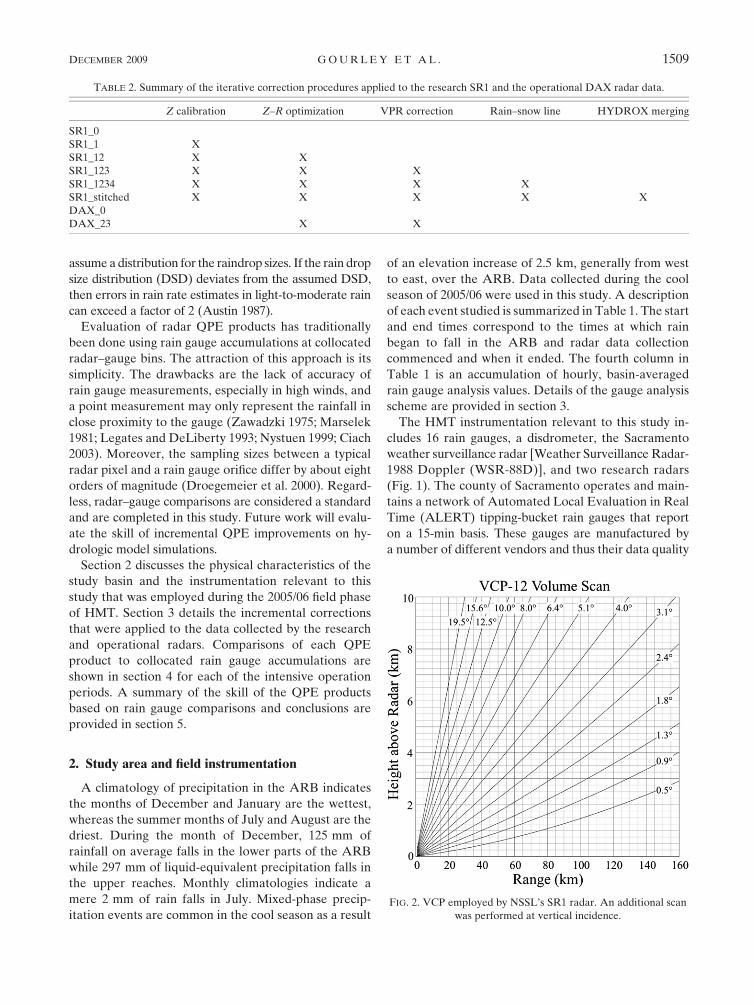
FIG. 2. VCP employed by NSSL’s SR1 radar. An additional scan
was performed at vertical incidence.
TABLE 2. Summary of the iterative correction procedures applied to the research SR1 and the operational DAX radar data.
Z calibration Z–R optimization VPR correction Rain–snow line HYDROX merging
SR1_0
SR1_1 X
SR1_12 X X
SR1_123 X X X
SR1_1234 X X X X
SR1_stitched X X X X X
DAX_0
DAX_23 X X
DECEMBER 2009 G O U R L E Y E T A L . 1509

must be carefully monitored. As part of the HMT ex-
periment, NOAA’s Earth System Research Laboratory’s
Physical Sciences Division (ESRL PSD) deployed nine
observing platforms in the vicinity of the ARB, providing
standard meteorological observations as well as 5-min
precipitation totals. Figure 1 shows 10 ALERT gauges
and five ESRL PSD gauges that were used to evaluate
remotely sensed QPE fields in section 4. Three of the
ESRL PSD gauges were manufactured by Met One
Instruments, Inc. They were heated and wind shielded.
The remaining two gauges, manufactured by Texas
Electronics, were deployed in lower elevations and were
neither heated nor wind shielded. All ESRL PSD gauges
were factory calibrated to within 0.25 mm. These gauges
are a subset from the entire network; their selection was
based on their close proximity to the ARB and the radar
coverage provided by the research radars. A Distromet
LTD model RD-80 disdrometer was used for radar cali-
bration and for optimizing the Z–R relation as described in
section 3. The Sacramento WSR-88D radar (DAX) is
72 km away from the basin outlet and 147 km from the
upper reaches of the ARB. Rainfall estimates derived
from DAX reflectivity measurements were used in this
study to compare with QPEs from the gap-filling, research
radars. ESRL PSD deployed an X-band polarimetric ra-
dar (HYDROX) having a 3.1-m-diameter antenna, a peak
transmit power of 30 kW, beamwidth of 0.98, gate spacing
of 150 m, and measurements out to a maximum range of
38.4 km. Additional characteristics of HYDROX (for-
merly XPOL) are provided in Martner et al. (2001). The
Shared Mobile Atmospheric Research and Teaching
Radar (SR1) was deployed for HMT at Forest Hill by
the National Severe Storms Laboratory (NSSL). SR1 is
a C-band Doppler radar having a 2.4-m-diameter antenna
with a maximum transmit power of 250 kW (Biggerstaff
et al. 2005). It has a 1.58 beam width, 125-m nominal range
gate spacing, and the maximum range was 150 km.
3. QPE processing
A substantial amount of processing SR1 reflectivity
measurements (Ze) was needed to yield QPEs with
FIG. 3. Hybrid scan lookup table developed for SR1 reflectivity data. The colors correspond to radar
elevation angles (in degrees) shown in the color bar. Entire network of ALERT rain gauges are shown as
blue triangles and ESRL PSD gauges are shown as red circles.
1510 J O U R N A L O F H Y D R O M E T E O R O L O G Y VOLUME 10
incremental corrections applied. The reader is referred
to Table 2 to quickly see the number of corrections ap-
plied for each QPE product. SR1 collected raw mea-
surements using volume coverage pattern (VCP) 12 with
an added scan at vertical incidence (Fig. 2). An initial
hybrid scan lookup table was computed based on modeled
beam heights for VCP 12 relative to a 30-m-resolution
digital elevation model (DEM). The intent of the hybrid
scan was to reduce the three-dimensional volume scans
to a two-dimensional reflectivity grid sampled closest to
the ground. Manual analysis of hybrid scan reflectivity
data revealed additional blockages that were unac-
counted for in the DEM. These blockages were a result
of trees and structures in close vicinity to the radar. The
hybrid scan lookup table was thus edited to assign higher
elevation angles to blocked radials. Figure 3 shows the
0.58 elevation angle was used for the lower portion of
the basin, whereas elevation angles as high as 3.18 were
needed to cover the entire basin. As will be seen in
section 4, the siting of SR1 in complex terrain with near-
by trees inhibited low-level coverage in the upper parts
of the ARB. The HYDROX radar scanning procedure
included sector scans at a 38 elevation tilt with a maxi-
mum range of 38.4 km, thus only 44% of the total North
Fork of the ARB (in its lower part) was covered by this
radar.
The first QPE product derived from SR1 data simply
converted hybrid scan reflectivity to rainfall rate (R)
using the default Z–R relation for the Next Generation
Weather Radars (NEXRADs):
Z 5 300R1.4, (1)
where the units for Z are mm6 m23 and R is mm h21. All
radar-based QPE products were sampled from polar
coordinates onto a 500-m-resolution Cartesian grid on
an hourly basis. This QPE product was subjected to no
corrections (hereafter SR1_0).
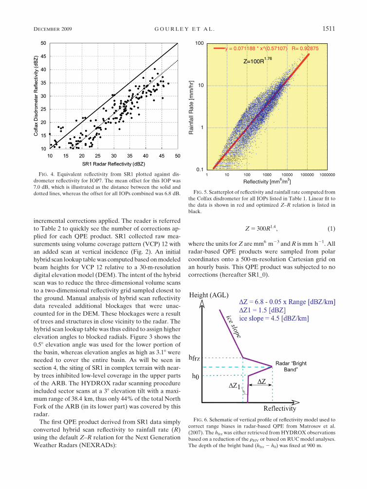
FIG. 4. Equivalent reflectivity from SR1 plotted against dis-
drometer reflectivity for IOP7. The mean offset for this IOP was
7.0 dB, which is illustrated as the distance between the solid and
dotted lines, whereas the offset for all IOPs combined was 6.8 dB. FIG. 5. Scatterplot of reflectivity and rainfall rate computed from
the Colfax disdrometer for all IOPs listed in Table 1. Linear fit to
the data is shown in red and optimized Z–R relation is listed in
black.
FIG. 6. Schematic of vertical profile of reflectivity model used to
correct range biases in radar-based QPE from Matrosov et al.
(2007). The hfrz was either retrieved from HYDROX observations
based on a reduction of the rHV or based on RUC model analyses.
The depth of the bright band (hfrz 2 h0) was fixed at 900 m.
DECEMBER 2009 G O U R L E Y E T A L . 1511

The first incremental correction applied to SR1 data
accounted for radar miscalibration using a disdrometer
as in Joss et al. (1968). The SR1 radar was initially
calibrated by injecting a signal into the receiver with
known strength. This approach did not account for the
combined calibration of the transmitter and receiver in
weather signals. The Colfax disdrometer was located
only 11.5 km away from SR1 (see Fig. 1). The close
proximity of the disdrometer to SR1 meant errors due to
horizontal advection and microphysical changes of hy-
drometeors below the altitude of radar sampling could
be safely neglected. The disdrometer used an electro-
mechanical transducer to measure each drop’s mo-
mentum, which is proportional to drop diameter. The
number density of drop diameters were then averaged
on a 5-min basis and converted to reflectivity values to
be comparable with radar-measured reflectivity values.
For each intensive observing period (IOP), reflectivity
computed from disdrometer data was compared to col-
located reflectivity measurements from SR1 every five
minutes. Figure 4 shows a scatterplot of disdrometer-to-
SR1 reflectivity data for IOP7. The mean offset of SR1
minus disdrometer reflectivity was 7.0 dB for this IOP,
indicating SR1 reflectivity was biased extremely high.
Similar plots were produced for each IOP and revealed
that the mean offset for all IOPs was 6.8 dB, with
a standard deviation of 1.3 dB. The stability of the cal-
ibration bias, despite its large absolute value, enabled us
to use the mean offset value of 6.8 dB for all IOPs. The
QPE product that has been corrected for radar mis-
calibration is hereafter referred to as SR1_1.
The second correction implemented on SR1 data con-
sidered deviations in the observed DSD from the assumed
DSD used to convert reflectivity to rainfall rate using (1).
Figure 5 shows a scatterplot of disdrometer-computed Z
and R for all IOPs listed in Table 1 combined. Least
FIG. 7. Comparison of (a) SR1_0, (b) SR1_1, (c) SR1_12, (d) SR1_123, (e) SR1_1234, (f) SR1_stitched, (g) DAX_0,
and (h) DAX_23 QPE products to hourly rain gauge accumulations for all IOPs listed in Table 1. Section 3 describes
each QPE product.
1512 J O U R N A L O F H Y D R O M E T E O R O L O G Y VOLUME 10

squares regression was used to fit a line to the data that
has the following form [with same units as Eq. (1)]:
Z 5 100R1.76. (2)
It should be noted that the use of disdrometer-computed
reflectivity to arrive at the provided formulation assumes
radar-based reflectivity is compatible, or calibrated, which
was done in the first step. Hypothetically speaking, the first
correction to the radar calibration factor could have been
superseded by directly comparing the uncalibrated SR1 Ze
to the disdrometer-measured R. However, this would have
made the Ze–R relation specific to the SR1 radar. As will
be shown later in this section, a more general Z–R relation
found with disdrometer data in (2) was also applied to
other radars, such as the operational DAX radar.
Although there may have been some variability in the
Z–R relation from event-to-event as reported in Matrosov
et al. (2007), a Pearson correlation coefficient of 0.93 with
a root-mean-square error (RMSE) of 1.8 mm hr21 was
found for disdrometer-computed R and Z using data for
all IOPs combined. The low DSD variability observed
on the ARB may have been specific to synoptically
forced orographic precipitation observed on the western
slopes of the Sierra Nevada and thus may not be expe-
rienced in other precipitation regimes. The coefficient in
(2) falls between the coefficients found for rainfall
characterized by a presence of a brightband (BB) and
nonbrightband (NBB) rainfall in Martner et al. (2008).
Moreover, R using (2) differs from rain rates computed
for BB rainfall by less than 15% for Z from 33–53 dBZ;
Z must be .46 dBZ to get agreement within 15% for R
computed for NBB rainfall. The low variance in our
disdrometer-measured R and agreement within 15% for
R computed for BB rainfall suggests a majority of ob-
servations during IOPs on the ARB was from rainfall
with a melting-layer signature, with a small contribution
from NBB rainfall. This assumption was verified by
subjectively analyzing time series plots of signal-to-noise
ratio as observed by an S-band profiling radar located at
Alta, California, in the ARB (not shown). Martner et al.
FIG. 7. (Continued)
DECEMBER 2009 G O U R L E Y E T A L . 1513

(2008) found melting-layer signatures to be present with
ice processes in deep clouds associated with synoptic-
scale forcing. This is consistent with the IOP planning
procedure that focused on events for study during strong
synoptic forcing. The QPE product that has been cor-
rected for radar miscalibration and used (2) for rain-rate
estimation is hereafter referred to as SR1_12. SR1 QPE
products hereafter relied on (2) for rain-rate estimation.
The next correction was designed to resolve range bia-
ses in QPE caused by the vertical variability of reflectivity
using the method described in Matrosov et al. (2007).
Figure 6 shows a modeled vertical profile of reflectivity
that has been parameterized to describe orographically
generated stratiform precipitation with a melting-layer
signature, or bright band. All parameters listed in blue
were manually adjusted based on HYDROX-observed
reflectivity profiles for IOP7 as well as a comparison to
collocated rain gauge accumulations. Although pre-
sented values of DZ and DZ1, which were used in this
study, are averages, one can expect that they may change
depending on conditions. For example, DZ1 could in-
crease with decreasing radar elevation angle because
longer path lengths in the melting layer would add more
melting-layer attenuation, which is generally more sig-
nificant than attenuation in rain (Matrosov 2008). The
only parameter that was adjusted in this study is the
freezing-level height (hfrz). These values were retrieved
either from HYDROX observations based on a reduc-
tion of the co-polar cross-correlation coefficient (rHV) or
Rapid Update Cycle (RUC) model analyses. HYDROX
rHV observations were used during the times at which
low-level scans intercepted the melting layer; otherwise,
values were taken directly from the RUC model on an
hourly basis. Provided the height of the radar measure-
ment, the model shown in Fig. 6 was used to extrapolate
measured reflectivity to represent values at the surface. It
should be noted that improvements are expected when
SR1 is upgraded with polarimetric diversity and can thus
use a line of sight rHV as opposed to using the measure-
ments from HYDROX. Reflectivity values were then
corrected for radar miscalibration and converted to rain-
fall rates using (2). This product is hereafter referred to as
SR1_123.
Analysis of the aforementioned freezing-level height
time series indicated mixed-phase precipitation affected
the ARB for all IOPs except IOP3. IOP7 was the coldest
event with freezing-level heights falling to 1.42-km MSL.
In this study, grid points receiving frozen precipitation
were identified by comparing terrain heights from the
DEM (see Fig. 1) to freezing-level heights on an hourly
basis. If the DEM height was greater than the freezing-
level height, then rain rates at those grid points were
simply set to zero. The rain–snow product, referred to
hereafter as SR1_1234, had the same values as SR1_123
but with rainfall rates set to zero at grid points above the
freezing layer.
The final correction to SR1 data merged rainfall rate
estimates from HYDROX with SR1. Reflectivity data
TABLE 3. Summary of the normalized bias computed for each IOP for each algorithm. Refer to Table 2 for the corrections that were made
to each product. The algorithm with the best performance for each IOP according to the statistic is denoted in boldface.
IOP1 IOP2 IOP3 IOP4 IOP5 IOP6 IOP7 IOP10 IOP11 IOP12
SR1_0 0.69 0.52 0.41 0.36 0.33 20.11 0.39 0.18 20.24 1.13
SR1_1 20.27 20.40 20.67 20.48 20.58 20.71 20.55 20.58 20.56 20.18
SR1_12 20.10 20.17 20.53 20.37 20.36 20.46 20.29 20.44 20.44 20.02
SR1_123 20.07 20.06 20.47 20.34 20.20 20.38 0.06 20.38 20.40 20.08
SR1_1234 20.07 20.06 20.47 20.34 20.20 20.38 0.06 20.38 20.40 20.08
SR1_stitched 20.02 20.08 20.41 20.26 20.07 20.38 0.04 20.30 20.31 20.16
DAX_0 20.70 20.71 20.47 20.53 20.70 20.82 20.75 20.73 20.88 20.59
DAX_23 20.31 20.29 20.22 20.34 20.26 20.49 20.10 20.49 20.72 20.30
TABLE 4. Same as Table 3 but for RMSE.
IOP1 IOP2 IOP3 IOP4 IOP5 IOP6 IOP7 IOP10 IOP11 IOP12
SR1_0 6.01 3.95 3.25 7.35 2.68 1.02 2.21 2.56 3.31 5.18
SR1_1 7.24 4.12 3.09 7.40 2.40 1.18 2.04 2.23 3.68 5.30
SR1_12 5.44 3.45 2.82 6.12 2.31 0.92 1.97 2.14 2.76 4.44
SR1_123 4.18 2.62 2.99 5.40 2.13 0.96 2.74 2.27 3.34 3.54
SR1_1234 4.18 2.62 2.99 5.40 2.13 0.96 2.74 2.27 3.34 3.54
SR1_stitched 3.88 2.42 3.03 4.09 2.05 1.04 2.44 2.33 3.52 3.03
DAX_0 3.68 3.45 4.08 8.30 2.91 1.08 2.33 2.42 3.63 4.35
DAX_23 2.49 2.56 2.89 3.96 1.95 1.12 2.11 1.94 2.99 3.01
1514 J O U R N A L O F H Y D R O M E T E O R O L O G Y VOLUME 10

from HYDROX were initially corrected for miscalibra-
tion using a corner reflector and then through reflectivity
comparisons observed by the Colfax disdrometer once
the radar was deployed in the field. Reflectivity data were
then corrected for attenuation losses using the polari-
metric method outlined in Matrosov et al. (2005), and
range effects were mitigated using the vertical profile of
the reflectivity model shown in Fig. 6 (Matrosov et al.
2007). Rainfall rates were estimated using the same Z–R
relation shown in (2). Consideration of frozen hydrome-
teors accumulating at the surface was not warranted with
HYDROX data as a result of its low-elevation siting at
468-m MSL and production of rainfall rates out to a
maximum range of 38 km. The merging technique simply
replaced SR1_1234 rain rates with HYDROX rain rates
at grid points where HYDROX data were available.
This product is hereafter referred to as SR1_stitched
(see Table 2 for a summary).
Rainfall estimates with two levels of correction were
produced using reflectivity measurements from the op-
erational NEXRAD in Sacramento called DAX. The
first product, hereafter referred to as DAX_0, was sim-
ilar to SR1_0 in that it is considered raw with no cor-
rections and relied on the default Z–R relation shown in
(1). In essence, the DAX_0 product approximates the
operational rainfall algorithm. Comparisons of DAX
reflectivity to disdrometer observations, which would be
needed for calibration, were problematic because of the
distance of 91 km between the two instruments. It is thus
assumed that the operational DAX radar was reason-
ably calibrated. Reflectivity comparisons from neigh-
boring NEXRADs were examined and showed no
significant biases (not shown). The second product used
the optimized Z–R relation shown in (2) and corrected
for range effects using the model illustrated in Fig. 6. In
this case, the freezing-level heights were used exclu-
sively from RUC model analyses. This product, here-
after referred to as DAX_23, represents a QPE product
derived from the operational radar network with cor-
rections applied that do not rely on experimental ob-
servations in the future but rather data available in an
operational setting.
A QPE product based on the 10 ALERT and five
ESRL PSD gauge reports shown in Fig. 1, referred to as
GAG_0, was analyzed for subjective comparison with
radar-based products. First, raw gauge reports were
quality controlled through manual, meticulous inspec-
tion of each station’s time series file covering each IOP.
Then, the 5- and 15-min gauge reports were aggregated
up to hourly accumulations, available at the top of each
hour. The gauge data were then sampled onto the 500-m-
resolution Cartesian grid using natural neighbor linear
interpolation (Akima 1978; Sibson 1981). The method
calculated area-based weights and produced an inter-
polated surface with continuous slope except at the gauge
locations where the quality-controlled gauge value was
used. The result of this interpolation scheme was a smooth
surface with sharp gradients, analogous to tent poles, at
TABLE 5. Same as Table 3 but for Pearson correlation coefficient.
IOP1 IOP2 IOP3 IOP4 IOP5 IOP6 IOP7 IOP10 IOP11 IOP12
SR1_0 0.36 0.14 0.23 0.04 0.01 0.29 0.15 20.05 20.06 0.02
SR1_1 0.34 0.12 0.18 0.05 20.02 0.28 0.11 20.05 20.08 20.02
SR1_12 0.40 0.18 0.24 0.06 0.04 0.31 0.17 20.01 20.03 0.04
SR1_123 0.45 0.28 0.18 0.05 0.24 0.33 0.12 20.04 20.03 0.16
SR1_1234 0.45 0.28 0.18 0.05 0.24 0.33 0.12 20.04 20.03 0.16
SR1_stitched 0.47 0.31 0.19 0.24 0.23 0.29 0.12 20.07 0.00 0.18
DAX_0 0.41 0.19 0.27 0.20 20.11 0.34 0.12 20.14 20.19 20.14
DAX_23 0.59 0.30 0.28 0.18 0.18 0.20 0.22 20.07 0.01 0.11
TABLE 6. Same as Table 3 but for number of nonzero radar–gauge pairs.
IOP1 IOP2 IOP3 IOP4 IOP5 IOP6 IOP7 IOP10 IOP11 IOP12
SR1_0 162 218 138 144 151 71 123 174 36 244
SR1_1 156 210 122 143 137 71 116 146 32 226
SR1_12 165 219 137 144 152 71 124 185 38 245
SR1_123 165 220 137 143 152 71 121 181 38 245
SR1_1234 165 220 137 143 152 71 121 181 38 245
SR1_stitched 162 212 136 147 155 69 124 181 37 249
DAX_0 158 200 74 148 155 54 117 154 24 243
DAX_23 165 218 79 148 173 71 125 187 38 251
DECEMBER 2009 G O U R L E Y E T A L . 1515

the gauge locations. The GAG_0 served as a benchmark
for subjective comparison purposes with the remotely
sensed, radar-based QPE products.
4. Results
The evaluation compared radar-based QPEs from the
research radars and the operational DAX radar to rain
gauge accumulations. QPEs from SR1, subject to in-
cremental corrections, and from uncorrected and cor-
rected DAX were plotted against hourly rain gauge
accumulations on a log scale at collocated grid points for
all IOPs combined (see Fig. 7). Radar–gauge pairs were
considered if both reports were nonzero. Each panel in
Fig. 7 indicates the normalized bias (NB; defined as the
sum of radar minus gauge accumulations divided by the
sum of the gauge accumulations), RMSE computed af-
ter the radar bias was removed, and Pearson correlation
coefficient. The highest skill in a given QPE product is
indicated with a normalized bias nearest 0.0 (in which
negative numbers indicate underestimation and positive
numbers indicate overestimation), lowest RMSE, and
highest correlation coefficient. In addition, we com-
puted the aforementioned skill metrics for each IOP
separately and reported those in Tables 3–6.
The SR1_0 product showed very little skill when
compared to rain gauge accumulations (Fig. 7a). Sig-
nificant overestimation occurred because of the extreme
6.8-dB miscalibration of the radar. When considering all
FIG. 8. Height of the hybrid scan beam heights (in m above MSL)
for (a) SR1 and (b) DAX. The ALERT and ESRL PSD gauges
used in the rain gauge evaluation are shown as blue triangles and
red circles, respectively. The ARB is outlined in red.
FIG. 9. Rainfall accumulation on the North Fork of the ARB for
all IOPs combined from (a) GAG_0, (b) DAX_23, and (c)
SR1_stitched. Refer to section 3 for detailed descriptions of each
rainfall product.
1516 J O U R N A L O F H Y D R O M E T E O R O L O G Y VOLUME 10

gauges for all IOPs, overestimation with a NB of 0.52, or
52%, occurred with SR1_0. When the radar was properly
calibrated, as was the case with the SR1_1 product, the
correlation coefficient remained unchanged, the RMSE
increased, and the NB became 20.43, indicating under-
estimation by 43%. Evidently, radar calibration alone did
not provide substantial improvements in skill to QPE
algorithms when an improper Z–R relation was used.
Optimizing the parameters in the Z–R relation in the
SR1_12 product, which required calibrated radar re-
flectivity data, resulted in substantial improvements in all
three scores. Further improvement in all scores was
gained in the SR1_123 product by implementing a range
correction procedure based on the modeled vertical
profile of reflectivity. These improvements were not en-
tirely unexpected; we optimized the ice slope parameter
illustrated in Fig. 6 using rain gauge comparisons for
IOP7. Evidently, the optimization was appropriate for
the other IOPs. The skill scores remained virtually un-
changed when consideration of the rain/snow line was
made in the SR1_1234 product. This was because the rain
gauges used in the analysis (see Fig. 1) were situated at
altitudes below the freezing level for most IOPs. Thus,
the SR1_1234 product was the same as the SR1_123
product in the raining regions. The final correction to
SR1 data, stitching together the SR1_1234 product with
HYDROX rain rates, resulted in modest improvements
in all three skill scores. The best scores we achieved after
applying all incremental corrections to reflectivity data
from merged, gap-filling radars were an NB of 20.18, an
RMSE of 2.92 mm, and Pearson correlation coefficient
of 0.47.
The uncorrected DAX QPE product, DAX_0, sub-
stantially underestimated gauge amounts, as noted with
an NB of 20.64 (Fig. 7g). The RMSE was lower than
with SR1_0 and SR1_1, and the correlation coefficient
was unexpectedly higher than all SR1 QPE products,
except SR1_stitched, with a value of 0.41. The applica-
tion of the optimized Z–R relation and vertical re-
flectivity correction improved the NB of DAX_23 to
20.32 and yielded the lowest RMSE (2.63 mm) and
highest correlation coefficient (0.52) of all radar-based
QPE products.
The unexpectedly high skill of DAX_23 relative to the
merged, gap-filling SR1_stitched product prompted us
to examine radar coverages over the ARB. A study by
Maddox et al. (2002) mapped WSR-88D radar coverages
over the conterminous United States and pointed out the
dearth of low-level coverage in the intermountain West.
Uncertainty in rain rates are expected to increase when
reflectivity is measured at higher altitudes and extrapo-
lated to represent surface values, even when reflectivity
was corrected using a modeled vertical profile of reflec-
tivity. Thus, one of the objectives of HMT was to evaluate
the improvement in QPE offered by research radars sit-
uated in mountainous terrain where WSR-88D beam
blockages are common. Beam heights of the hybrid scan
(in meters above MSL) were computed for SR1 and DAX
and are illustrated in Fig. 8.
Figure 8a shows that two of the rain gauges, located at
Bear River at Rollins Reservoir (BRE) and Alta (ATA),
were situated in blocked radials from SR1’s perspective.
The SR1_stitched QPE product replaced SR1_1234
rain rates with those estimated by HYDROX out to a
maximum range of 38 km. The HYDROX radar pro-
vided better coverage over several gauges in the lower
part of the basin, which helped to explain the improve-
ment realized with the SR1_stitched product over
SR1_1234. In addition, HYDROX is an X-band radar
with polarimetric capabilities, which provided a mecha-
nism to account for attenuation losses. We also com-
puted rainfall accumulations for GAG_0, DAX_23, and
SR1_stitched for all IOPs combined (Fig. 9). Subjective
comparison of the accumulations in Fig. 9 indicates the
DAX_23 and GAG_0 products captured the increasing
gradient of precipitation in the upper parts of the basin
that reach a maximum and then decrease at the crests.
There appears to be a bias between the gauge analysis
field and the DAX_23 product. The SR1_stitched prod-
uct, on the other hand, illustrates qualitative agreement
with the GAG_0 analysis but only in regions where there
were no blocked radials from SR1’s perspective.
To quantify the effect of radar coverage on QPE skill,
the normalized bias has been computed in Fig. 10 as
a function of radar sampling height in meters above MSL
over each rain gauge location for all IOPs combined.
Figures 10a–c show the normalized bias is particularly
dependent on radar sampling height. In comparing Figs.
10c,d, it is apparent that the VPR corrections reduced
the overestimation that was present from 3.5–6.5 km in
Fig. 10c and improved the underestimation problem above
6.5 km. Further improvements are noted in the vertical
error structure following the inclusion of HYDROX
data in the QPE product (Fig. 10f). The most significant
improvements occurred at sampling heights of 1.1 and
4.5 km; the gauges at these locations were FHL and
ATA, respectively. Figure 8a shows ATA was situated
directly in a blocked radial from SR1, which appar-
ently degraded the performance of the QPE value there.
FHL was within 1 km distance from the SR1 site, which
placed it within the near field of the radar and also
subjected it to ground clutter removal procedures. Re-
placing the SR1 rainfall estimates with those measured
from HYDROX in regions within the near field of the
antenna led to a better QPE product over the FHL
gauge site.
DECEMBER 2009 G O U R L E Y E T A L . 1517

Comparison of Figs. 10g,h shows the application of an
optimized Z–R relation found with disdrometer data, and
a VPR correction method that was developed on SR1
data resulted in a skillful, but negatively biased, QPE
product from the operational DAX radar. In fact, the
normalized bias has less dependence on height than
compared to the final QPE product from the research
radars (see Figs. 10f,h). This finding indicates the pro-
cedures developed on the research radars apply directly
to a NEXRAD situated as far as 147 km away. Moreover,
the most skillful QPE product coming from the DAX
radar is explained by the superior coverage the NEXRAD
provides over the upper parts of the basin. The terrain
generally rises from west to east along with the radar
beams from DAX. Most importantly, there are no nearby
trees or obstructions to block the DAX visibility over the
ARB, which was certainly the case with the SR1 radar
siting. This finding indicates careful consideration of
nearby blockages due to terrain and trees must be taken
when siting a research radar that is intended to be used as
a gap-filling radar.
5. Summary and conclusions
The North Fork of the American River Basin (ARB)
in California was heavily instrumented with in situ and
remote sensing instruments during NOAA’s Hydrome-
teorological Testbed experiment beginning in the winter
of 2005/06. A network of 16 rain gauges, an X-band
polarimetric radar (HYDROX), a C-band radar (SR1),
an S-band NEXRAD radar at Sacramento (DAX), and
a disdrometer were used in this study to quantify the skill
in improvements to radar-based QPE products using
hourly rain gauge accumulations as reference rainfall.
The correction procedures have been applied in an it-
erative fashion to examine their effects on gap-filling,
research radars having differing radar frequencies and
polarization states. Moreover, the corrections have been
adapted and applied to a nearby NEXRAD radar to
determine the transferability of the methods to opera-
tional rainfall rate estimation algorithms.
The evaluation indicated calibration of radar reflec-
tivity resulted in no significant improvements to rainfall
fields, as computed using the default NEXRAD relation,
compared to those derived from raw, uncorrected re-
flectivity data. However, after the parameters used to
convert reflectivity data to rainfall rates were found with
disdrometer measurements, better agreement with col-
located rain gauge accumulations resulted. This result
indicates that the effectiveness of radar calibration de-
pends on simultaneous optimization of the Z–R relation.
Modest improvements to radar-based rainfall fields were
FIG. 10. Same as Fig. 7 but for normalized bias plotted as a function of radar sampling height in meters above MSL
at each gauge site for (a) SR1_0, (b) SR1_1, (c) SR1_12, (d) SR1_123, (e) SR1_1234, (f) SR1_stitched, (g) DAX_0,
and (h) DAX_23 QPE products.
1518 J O U R N A L O F H Y D R O M E T E O R O L O G Y VOLUME 10

realized through the application of a range-correction
procedure using a modeled vertical profile of reflectivity
and by using measurements from the HYDROX radar.
In comparing all the QPE products, the lowest RMSE of
2.63 mm and highest Pearson correlation coefficient of
0.52 was achieved with data measured by the NEXRAD
located near Sacramento, CA, with corrections that
accounted for the variability of reflectivity with height
and used optimized parameters in the Z–R relation.
SR1_stitched, which had a normalized bias of 20.18,
indicating 18% underestimation, an RMSE of 2.92 mm
(with the bias removed), and a Pearson correlation co-
efficient of 0.47, provided an improvement over the
DAX_23 product in terms of the bias (20.18 versus
20.32) but did not provide improvements in terms of the
RMSE or the correlation (2.92 versus 2.62 mm and 0.47
versus 0.52, respectively). First, this result demonstrated
the transferability of QPE correction methods de-
veloped in complex terrain for research radars to an
operational NEXRAD. These results prompted us to
examine the operational versus experimental radar cov-
erages over the ARB. SR1 had several blocked radials by
nearby trees creating a ‘‘spoked’’ appearance in QPE
fields. The blockages were mitigated in the lower part of
the basin by replacing QPE values with those measured
by the HYDROX radar. However, the maximum range
of HYDROX was 38 km, which meant QPE products
from the merged, research radars relied exclusively on
data from SR1 in the upper part of the basin. DAX had at
least as good or even better coverage in these regions,
even at a maximum distance of 147 km away, because it
did not suffer from the tree blockage problems experi-
enced by SR1. Plus, the terrain in the ARB generally
increases in elevation from west to east in a similar
manner that the DAX beam heights increase with range.
It should be noted, however, that the low-level coverage
offered by DAX is unusually good compared to typical
radar coverages in the intermountain West, as seen in
Maddox et al. (2002). Lastly, this study points out that
careful consideration of radar sitings for gap-filling radars
in study basins must be taken to avoid blockages due to
nearby terrain, structures, and trees.
Acknowledgments. The authors have benefitted from
many discussions about radar-based quantitative pre-
cipitation estimation techniques with Pedro Restrepo
and David Kitzmiller (NOAA/NWS/OHD), Brooks
Martner and David Kingsmill (CIRES, University of
Colorado and NOAA/ESRL/PSD), and Marty Ralph
(NOAA/ESRL/PSD). Much of the deployment costs for
the SR1 participation in the Hydrometeorological Test-
bed experiment were provided by NOAA/OAR. The
authors also would like to thank NOAA/ESRL/PSD and
NOAA/NWS/OHD for providing internal reviews of
FIG. 10. (Continued)
DECEMBER 2009 G O U R L E Y E T A L . 1519

this manuscript. Comments from three anonymous re-
viewers helped to improve the clarity and analysis pro-
cedures used in this manuscript.
REFERENCES
Akima, H., 1978: A method for bivariate interpolation and smooth
surface fitting for irregularly distributed data points. ACM
Trans. Math. Software, 4, 148–159.
Andrieu, H., and J. D. Creutin, 1995: Identification of vertical
profiles of radar reflectivities for hydrological applications
using an inverse method. Part I: Formulation. J. Appl. Meteor.,
34, 225–239.
Atlas, D., 2002: Radar calibration: Some simple approaches. Bull.
Amer. Meteor. Soc., 83, 1313–1316.
Austin, P. M., 1987: Relation between measured radar reflectivity
and surface rainfall. Mon. Wea. Rev., 115, 1053–1070.
——, and A. Bemis, 1950: A quantitative study of the ‘‘bright
band’’ in radar precipitation echoes. J. Meteor., 7, 145–151.
Battan, L. J., 1976: Vertical air motions and the Z-R relation.
J. Appl. Meteor., 15, 1120–1121.
Bellon, A., G. Lee, and I. Zawadzki, 2005: Error statistics of VPR
corrections in stratiform precipitation. J. Appl. Meteor., 44,998–1015.
Biggerstaff, M. I., and Coauthors, 2005: The Shared Mobile At-
mospheric Research and Teaching radar: A collaboration to
enhance research and teaching. Bull. Amer. Meteor. Soc., 86,1263–1274.
Ciach, G. J., 2003: Local random errors in tipping-bucket rain
gauge measurements. J. Atmos. Oceanic Technol., 20, 752–759.
Dotzek, N., and T. Fehr, 2003: Relation between precipitation rates
at the ground and aloft-A modeling study. J. Appl. Meteor., 42,
1285–1301.
Droegemeier, K. K., and Coauthors, 2000: Hydrological aspects of
weather prediction and flood warnings: Report on the ninth
prospectus development team of the U.S. Weather Research
Program. Bull. Amer. Meteor. Soc., 81, 2665–2680.
Germann, U., and J. Joss, 2002: Mesobeta profiles to extrapolate
radar precipitation measurements above the Alps to the
ground level. J. Appl. Meteor., 41, 542–557.
Joss, J., and A. Waldvogel, 1990: Precipitation measurements and
hydrology. Radar in Meteorology, D. Atlas, Ed., Amer. Me-
teor. Soc., 577–606.
——, and R. Lee, 1995: The application of radar-gauge compari-
sons to operational precipitation profile corrections. J. Appl.
Meteor., 34, 2612–2630.
——, J. C. Thams, and A. Waldvogel, 1968: The accuracy of daily
rainfall measurements by radar. Proc. 13th Radar Meteorol-
ogy Conf., Montreal, QC, Canada, Amer. Meteor. Soc.,
448–451.
Kitchen, M., and P. M. Jackson, 1993: Weather radar performance
at long range—Simulated and observed. J. Appl. Meteor., 32,
975–985.
——, R. Brown, and A. G. Davies, 1994: Real-time correction of
weather radar data for the effects of bright band, range and
orographic growth in widespread precipitation. Quart. J. Roy.
Meteor. Soc., 120, 1231–1254.
Legates, D. R., and T. L. DeLiberty, 1993: Precipitation mea-
surement biases in the United States. Water Resour. Bull., 29,
855–861.
Maddox, R. A., J. Zhang, J. J. Gourley, and K. W. Howard, 2002:
Weather radar coverage over the contiguous United States.
Wea. Forecasting, 17, 927–934.
Marselek, J., 1981: Calibration of the tipping-bucket raingage.
J. Hydrol., 53, 343–354.
Martner, B. E., K. A. Clark, S. Y. Matrosov, W. C. Campbell, and
J. S. Gibson, 2001: NOAA/ETL’s polarization-upgraded X-band
‘‘hydro’’ radar. Preprints, 30th Int. Conf. on Radar Meteorology,
Munich, Germany, Amer. Meteor. Soc., P3.5. [Available online
at http://ams.confex.com/ams/pdfpapers/21364.pdf.]
——, S. E. Yuter, A. B. White, S. Y. Matrosov, D. E. Kingsmill, and
F. M. Ralph, 2008: Raindrop size distributions and rain char-
acteristics in California coastal rainfall for periods with and
without a radar bright band. J. Hydrometeor., 9, 408–425.
Matrosov, S. Y., 2008: Assessment of radar signal attenuation
caused by melting hydrometeor layer. IEEE Trans. Geosci.
Remote Sens., 46, 1039–1047.
——, D. E. Kingsmill, B. E. Martner, and F. M. Ralph, 2005: The
utility of X-band polarimetric radar for quantitative estimates
of rainfall parameter. J. Hydrometeor., 6, 248–262.
——, K. A. Clark, and D. E. Kingsmill, 2007: A polarimetric radar
approach to identify rain, melting-layer, and snow regions for
applying corrections to vertical profiles of reflectivity. J. Appl.
Meteor. Climatol., 46, 154–166.
Nystuen, J. A., 1999: Relative performance of automatic rain gauges
under different rainfall conditions. J. Atmos. Oceanic Technol.,
16, 1025–1043.
Ryzhkov, A. V., S. E. Giangrande, V. M. Melnikov, and T. J. Schuur,
2005: Calibration issues of dual-polarization radar measure-
ments. J. Atmos. Oceanic Technol., 22, 1138–1155.
Seo, D.-J., J. P. Breidenbach, R. Fulton, D. Miller, and
T. O’Bannon, 2000: Real-time adjustment of range-dependent
biases in WSR-88D rainfall estimates due to nonuniform
vertical profile of reflectivity. J. Hydrometeor., 1, 222–240.
Sibson, R., 1981: A brief description of natural neighbor in-
terpolation. Interpreting Multivariate Data, V. Barnett, Ed.,
Wiley, 21–36.
Smith, C. J., 1986: The reduction of errors caused by bright bands in
quantitative rainfall measurements made using radar. J. At-
mos. Oceanic Technol., 3, 129–141.
Vignal, B., H. Andrieu, and J. D. Creutin, 1999: Identification of
vertical profiles of reflectivity from volume scan radar data.
J. Appl. Meteor., 38, 1214–1228.
Wilson, J., and E. Brandes, 1979: Radar measurement of rainfall—A
summary. Bull. Amer. Meteor. Soc., 60, 1048–1058.
Zawadzki, I. I., 1975: On radar-raingauge comparison. J. Appl.
Meteor., 14, 1430–1436.
1520 J O U R N A L O F H Y D R O M E T E O R O L O G Y VOLUME 10


