
A S H R A E J O U R N A L a s h r a e . o r g S E P T E M B E R 2 0 1 71 8
TECHNICAL FEATURE
Ellen Franconi, Ph.D., is energy analytics manager at the Rocky Mountain Institute in Boulder, Colo., and vice chair of SPC 209, Energy Simulation Aided Design for Buildings Except Low-Rise Residential Buildings. David Jump, Ph.D., P.E., is project manager at kW Engineering in Oakland, Calif.
BY ELLEN FRANCONI, PH.D., BEMP, MEMBER ASHRAE; DAVID JUMP, PH.D., P.E., MEMBER ASHRAE
Leveraging Smart Meter Data & Expanding ServicesIncreasingly, states are rolling out installations of smart meters for homes and busi-nesses. These meters represent the first phase in the evolution to a smart grid that uses digital technology to improve electric delivery system reliability, flexibility, and efficiency. Installations of smart meters for natural gas are also on the rise. As the deployment of smart meters grows, energy service providers will have access to a much richer data set over a much larger population of buildings.
Widely available interval data and recent advances in
computing power are fostering the development of new
technologies that streamline data collection and per-
form advanced analytics. The approach supports energy
performance assessment by time of day. It underlies
next generation measurement and verification (M&V)
methods, which we refer to as advanced M&V. Advanced
M&V has advantages over traditional regression-
based billing analysis, including more rapid feedback,
improved savings resolution, and increased model
accuracy due to many more data points. In addition, the
same data and analytics can be applied to identify oper-
ational abnormalities, which can support fruitful, lon-
ger-term customer engagement. These developments
provide an opportunity for energy service providers to
leverage smart meter data and advanced M&V to inform
and expand building efficiency projects and services.
The application of advanced M&V methods is more
complex than typical whole-building M&V methods
using monthly billing data. Interval data M&V models
include new forms of linear regression models that
incorporate time indicator variables. In addition, as the
time interval becomes smaller, the presence of autocor-
relation in the data increases, which impacts savings
uncertainty and necessitates its assessment. Applying
advanced M&V methods can have added benefit if oper-
ational improvement savings can be determined with
sufficient accuracy to be discernible using whole build-
ing data. In this article, we investigate these consider-
ations through a case study.
M&V MethodsIn the late 1980s, the International Performance
Measurement and Verification Protocol (IPMVP)
©ASHRAE www.ashrae.org. Used with permission from ASHRAE Journal. This article may not be copied nor distributed in either paper or digital form without ASHRAE’s permission. For more information about ASHRAE, visit www.ashrae.org.

S E P T E M B E R 2 0 1 7 a s h r a e . o r g A S H R A E J O U R N A L 1 9
TECHNICAL FEATURE
established an industry-accepted framework for M&V,
which includes four options for determining verified
savings. Performing M&V using whole-building data to
develop empirical models aligns with an IPMVP Option
C approach. Option C involves developing an M&V
model from baseline period whole building energy use
data and independent variables, then projecting the
baseline energy use into the post-install period condi-
tions. Savings are determined by subtracting the mea-
sured post-installation period use from the adjusted
baseline use.1
In the 1990s, ASHRAE began developing Guideline
14, Measurement of Energy, Demand, and Water Savings, to
provide procedures for using measured data to verify
savings.2 At the same time, ASHRAE initiated Research
Project 1050 (RP 1050), which created the inverse model-
ing toolkit (IMT). The IMT includes change-point mod-
els, which are piece-wise linear regression models with
each segment meeting at a common point.3 The IMT is
commonly applied with Option C using monthly utility
billing data and corresponding average monthly tem-
peratures or heating and cooling degree days. It provides
a simple and powerful approach for understanding the
weather dependence of building energy use, but without
temporal considerations.
Recent developments in interval data M&V model-
ing include new forms of linear regression models that
incorporate time indicator variables. For example, the
time-of-week and temperature (TOWT) model devel-
oped for demand response applications4 considers the
time of the week as well as the ambient temperature
as influences on energy use. The TOWT model cap-
tures the nonlinear relationship between outdoor air
temperature and load by dividing temperatures into
many intervals and then fitting a piecewise linear and
continuous temperature dependence. This means that
for one year of hourly data, the TOWT model would
include 168 (hours in a week) linked regressions; each
developed from at least 52 data points (8,760 hours in
a year).
A challenge for Option C applications is ensuring
that the anticipated project savings are “discernable.”
Guideline 14 requires that savings be stated within
±50% at the 68% confidence level to comply. Efficiency
project stakeholders (owners, financiers, and service
providers) would certainly desire more stringent cri-
teria. One way to ensure savings meet uncertainty
criteria is to develop accurate energy models for use in
the analysis. This is one area where the interval data
approach is advantageous over the monthly billing data
approach.
Assessing Savings Uncertainty Since actual savings can only be estimated and not
compared with a directly measured value, we discuss
the quality of our savings estimations in terms of their
uncertainty. Uncertainty is an expression of the prob-
ability or confidence with which an estimate is within
specified limits of the true value. As will be shown, the
accuracy with which we can model the baseline period
energy use has a direct effect on the uncertainty of our
savings estimate.
Monthly models are usually developed using ordinary
least squares regressions and 12 data points. Savings
must be large to be discernable above the “noise” (ran-
dom error of the regression model). For models devel-
oped from monthly data, this concern led to the rule-of-
thumb that savings must be at least 10% or 15% of annual
energy use.
Interval data converted to hourly or daily data pro-
vide orders of magnitude more data than monthly. As a
general rule, the more data used to develop regression
models, the more accurate the model. However, as the
time interval becomes smaller, the presence of autocor-
relation in the data increases. This reduces the inde-
pendence of the data points and serves to increase the
savings uncertainty, as discussed below.
Baseline model accuracy is assessed by metrics that
quantify their random and bias error. The bias error
shows how much the model under- or over-predicts
the total actual energy consumed in the model train-
ing period, and should be zero, or extremely small. The
random error indicates how well the model follows the
usage patterns of the actual data; good models follow
these patterns very closely. The metric most commonly
used to quantify its random error is the root mean
squared error (RMSE), or the coefficient of variation of
the RMSE (CV[RMSE]), which is the RMSE divided by the
average baseline energy use.
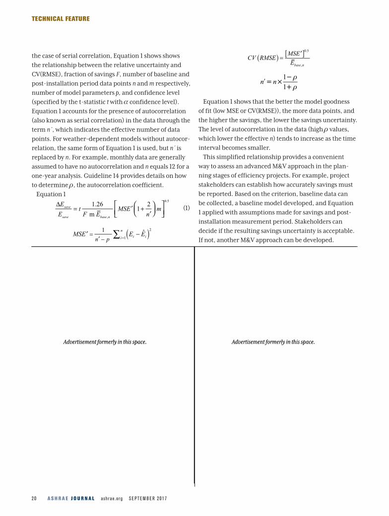
ASHRAE Guideline 14-2014 provides a simplified
approach to estimate savings uncertainty for two cases:
1) weather-dependent linear models from data that
are not serially correlated, and 2) weather-dependent
linear models from data that are serially correlated. In
A S H R A E J O U R N A L a s h r a e . o r g S E P T E M B E R 2 0 1 72 0
CV RMSEMSE
Ebase n
( ) =′[ ]0 5.
,
′= ×−+
n n1
1
ρρ
Equation 1 shows that the better the model goodness
of fit (low MSE or CV(RMSE)), the more data points, and
the higher the savings, the lower the savings uncertainty.
The level of autocorrelation in the data (high r values,
which lower the effective n) tends to increase as the time
interval becomes smaller.
This simplified relationship provides a convenient
way to assess an advanced M&V approach in the plan-
ning stages of efficiency projects. For example, project
stakeholders can establish how accurately savings must
be reported. Based on the criterion, baseline data can
be collected, a baseline model developed, and Equation
1 applied with assumptions made for savings and post-
installation measurement period. Stakeholders can
decide if the resulting savings uncertainty is acceptable.
If not, another M&V approach can be developed.
the case of serial correlation, Equation 1 shows shows
the relationship between the relative uncertainty and
CV(RMSE), fraction of savings F, number of baseline and
post-installation period data points n and m respectively,
number of model parameters p, and confidence level
(specified by the t-statistic t with confidence level).
Equation 1 accounts for the presence of autocorrelation
(also known as serial correlation) in the data through the
term n´, which indicates the effective number of data
points. For weather-dependent models without autocor-
relation, the same form of Equation 1 is used, but n´ is
replaced by n. For example, monthly data are generally
assumed to have no autocorrelation and n equals 12 for a
one-year analysis. Guideline 14 provides details on how
to determine r, the autocorrelation coefficient.
Equation 1
∆
= ′ +′
E
Et
F EMSE
nmsave
save base n
1 261
20 5
.
,
.
m (1)
MSE E En p
i ii
n′ −( )=
′ − =∑1 2
1 ˆ
TECHNICAL FEATURE
Advertisement formerly in this space. Advertisement formerly in this space.Advertisement formerly in this space. Advertisement formerly in this space.

Advertisement formerly in this space.Advertisement formerly in this space.

A S H R A E J O U R N A L a s h r a e . o r g S E P T E M B E R 2 0 1 72 2
models for each site using monthly, daily, and hourly
intervals for one year of data. We aimed to demonstrate a
streamlined approach to evaluate the M&V model uncer-
tainty and verified savings across the portfolio. The selected
form of the monthly model was a four-parameter (4p)
change point linear regression since it provided the best
data fit overall for the sites. Commercial software that
applies the IMT algorithms was used to develop the regres-
sions. The selected daily and hourly data models were the
LBNL TOWT4 regressions developed using the Universal
Translator 3.0 (UT3)tool.5 We performed general quality
assurance procedures but did not develop site-specific data
filters to improve regression fit on a case-by-case basis. We
determined the savings uncertainty for each model using
Equation 1, assuming the same duration for the baseline
and post-installation periods (m = n).
Figure 1 presents normalized monthly energy use for
each site over the calendar year. The sites are ordered
from largest to smallest (dark to light lines). Floor areas
range from 3,500,000 ft2 to 80,000 ft2 (325 161 m2 to
7432 m2). The figure indicates magnitude, range, and
seasonal variations across the data set. Many of the
buildings use some electric heat and a few receive cool-
ing from a district chilled water loop, resulting in many
of the buildings’ winter month electric use exceeding
summer month electric use.
Figure 2 shows the 4p regression plots developed using
3.00
2.50
2.00
1.50
1.00
0.50
0.00
kWh/
ft2 ·Mon
th
5 6 7 8 9 10 11 12 1 2 3 4Month
3.00
2.50
2.00
1.50
1.00
0.50
0.00
Elec
tricit
y Con
sum
ption
(kW
h/ft2 ·M
onth
)
10 30 50 70 90Monthly Average Outdoor Air Temperature (°F)
FIGURE 1 Monthly electricity consumption. FIGURE 2 Monthly 4P change point models.
This methodology is straightforward to apply; however, it
was developed based on linear methods assuming normal
distributions and independence of data. While the cor-
rection for autocorrelation helps, M&V models are being
developed with complex algorithms that are nonlinear in
nature. Advanced M&V algorithms include names such as
vector machines, neural networks, and machine learning.
Often these methods are proprietary. Methods for quantify-
ing savings uncertainty using these algorithms are more
complicated and are an area of current research.
Example Case Study We applied the Guideline 14 methods to a portfolio
subset that included whole-building interval data for
17 large commercial buildings located in climate zone
5a. Our client sought to understand the benefits of a
streamlined advanced M&V approach applied across
a large group of projects emphasizing operational
improvements. The client wanted to know how precisely
an Option C M&V model could determine savings prior
to embarking on scaled implementation. Should the
Option C approach not meet their accuracy require-
ments, they would explore a different M&V approach
or consider a service-based business model instead of
offering a performance guarantee.
We investigated the improvements in accuracy realized
from an advanced M&V approach by developing three
1 2 3 4 5 6 7 8 9 10 11 12 13 14 15 16 17
SITESLargest
Smallest
TECHNICAL FEATURE

S E P T E M B E R 2 0 1 7 a s h r a e . o r g A S H R A E J O U R N A L 2 3
monthly data. They indicate the varying temperature
dependence of electricity use for each site in the port-
folio. The slopes on either side of the change point are
indicative of the relative cooling and heating system
efficiencies of the modeled building. The change point
indicates the building balance point temperature above
or below which space conditioning begins. No attempt
was made to graph and present the annual data for the
interval data or more complex TOWT models. However,
their “energy signatures” can provide more detailed
insights by capturing load shape trends, which may be
best assessed through automated statistical methods or
machine learning techniques due to voluminous data
processing.
The regression statistics and auto-correlation val-
ues determined for the three models for each site are
presented in Table 1. In general, the regression models
developed with more granular data have larger residu-
als relative to the predicted value as indicated by their
TABLE 1 M&V electricity models regression statistics and example results.
MONTHLY 4-P CHANGE POINT MODEL DAI LY TOWT MODEL HOURLY TOWT MODEL
R2 CV n r n´ U (90% CI)
R2 CV n r n´ U (90% CI)
R2 CV n r n´ U (90% CI)
Site 1 0.9 2% 12 0 12 1.7% 0.87 10% 365 0.35 177 1.6% 0.92 17% 8,782 0.87 588 1.4%
Site 2 0.96 4% 12 0 12 3.2% 0.92 9% 364 0.20 242 1.2% 0.84 19% 8,758 0.83 815 1.3%
Site 3 0.71 9% 12 0 12 6.8% 0.66 14% 352 0.71 59 3.9% 0.76 24% 8,471 0.95 233 3.3%
Site 4 0.87 7% 12 0 12 4.8% 0.74 20% 365 0.71 61 5.4% 0.78 33% 8,782 0.95 242 4.5%
Site 5 0.94 12% 12 0 12 8.5% 0.89 21% 364 0.13 278 2.6% 0.84 40% 8,603 0.77 1,104 2.5%
Site 6 0.99 5% 12 0 12 3.9% 0.94 15% 364 0.34 180 2.3% 0.85 24% 8,758 0.86 650 1.9%
Site 7 0.82 9% 11 0 11 7.4% 0.57 26% 364 0.71 61 7.0% 0.61 33% 8,758 0.91 395 3.4%
Site 8 0.94 11% 12 0 12 8.1% 0.81 22% 366 0.71 61 5.9% 0.77 28% 8,782 0.95 242 3.7%
Site 9 0.84 8% 12 0 12 6.0% 0.90 9% 365 0.17 258 1.2% 0.91 17% 8,782 0.81 918 1.2%
Site 10 0.98 6% 12 0 12 4.3% 0.92 16% 365 0.13 281 2.0% 0.80 32% 8,782 0.83 824 2.3%
Site 11 0.89 10% 12 0 12 6.9% 0.70 23% 365 0.28 205 3.3% 0.63 44% 8,782 0.78 1,065 2.8%
Site 12 0.97 4% 12 0 12 2.8% 0.89 10% 364 0.31 192 1.5% 0.78 21% 8,759 0.79 1,055 1.4%
Site 13 0.96 8% 12 0 12 5.7% 0.86 17% 356 0.11 287 2.1% 0.74 39% 8,567 0.77 1,114 2.4%
Site 14 0.81 20% 12 0 12 14.2% 0.59 31% 364 0.72 59 8.6% 0.61 42% 8,758 0.91 414 4.3%
Site 15 0.98 9% 12 0 12 6.2% 0.86 24% 364 0.31 192 3.7% 0.71 53% 8,758 0.82 860 3.7%
Site 16 0.98 9% 12 0 12 6.2% 0.74 19% 364 0.38 162 3.2% 0.71 33% 8,758 0.80 970 2.2%
Site 17 0.95 7% 12 0 12 5.0% 0.80 17% 364 0.19 247 2.3% 0.72 33% 8,758 0.83 811 2.4%
higher coefficient of variation (CV) and lower R-squared
values. As indicated, the autocorrelation coefficient is
zero for monthly data. For some sites, the level of auto-
correlation was determined to be significant for the
daily and hourly utility data, which results in the effec-
tive number of independent data points being much less
than the actual number of data points. The uncertainty
values, reported for the 90% confidence interval, are rel-
ative to the baseline annual energy consumption (deter-
mined by multiplying both sides of Equation 1 by F, the
savings fraction). We refer to these values as the baseline
energy use uncertainty fraction.
A comparison between the different interval data
model fit is presented in Figure 3 for two sites. The Site 4
interval data models provided little or no improvement
in accuracy due to high autocorrelation and actual-
to-model data variance. As indicated in the chart, the
hourly data model for Site 4 poorly predicted the actual
data for swing season months possibly due to changes
TECHNICAL FEATURE

A S H R A E J O U R N A L a s h r a e . o r g S E P T E M B E R 2 0 1 72 4
in seasonal equipment scheduling. The model accuracy
improved the most with interval data for Site 9. For this
site, the interval data had limited autocorrelation and
the model had a relatively low CV.
Figure 4 presents the calculated uncertainty for a
range of confidence intervals for the monthly, daily,
and hourly regression models for each site. The values
indicate the inaccuracies introduced by the M&V model
in predicting performance. The results show that the
uncertainty is reduced on average by 40% to 60% if using
a daily data model instead of a monthly data model with
the most impact seen at higher confidence intervals.
Uncertainty is reduced further for hourly models—on
average an additional 25% reduction relative to the daily
model across all confidence intervals.
The baseline energy uncertainty fractions shown in
Figure 4 can be compared against the anticipated project
savings fraction to assess if the M&V approach is effec-
tive for verifying project savings using whole-building
electric data. Since the energy services will be offered
across a portfolio of buildings, it makes sense to quantify
the aggregated uncertainty of the data set. Since each
building is unique from the next, the fractional uncer-
tainty across the portfolio is determined using Equation
2, where ∆E is the savings uncertainty and N is the num-
ber of buildings in the portfolio.
Equation 2.
∆=
∆( )=
=
∑E
E
E
E
save portfolio
save portfolio
save ii
N
save ii
,
,
,
,
2
1
1
NN
∑ (2)
Figure 5 shows the uncertainty expressed in terms of
the anticipated savings. Our client estimates the range
of project savings to fall between 5% and 15%. In the fig-
ure, the plot area upper bound is based on a 5% portfolio
savings while the lower bound is based on 15% portfolio
savings for a range of confidence intervals. The results
show that the accuracy of verifying savings is noticeably
improved using interval data.
DiscussionIn our analysis, Guideline 14 equations quantified the
uncertainty associated with the baseline M&V models.
Developing models using shorter time interval data did
drive down uncertainty—a trend expected for good mod-
els. The presence of autocorrelation greatly reduced the
number of independent data points. Instead of going
FIGURE 3 Comparison between Site 4 and Site 9 M&V model data fit.
W/ft
2
Jun Jul Aug Sep Oct Nov Dec Jan Feb Mar Apr May
1.20
1.00
0.80
0.60
0.40
0.20
0.00
kWh/
ft2 ·Mon
th
Monthly80
70
60
50
40
30
20
10
0
Tem
pera
ture
(°F)
Site 4 Site 4 Model Site 9 Site 9 Model Temperature
2015 | 2016
Mar 1 Mar 8 Mar 15 Mar 22 Mar 29
Wh/
ft2 ·Day
Daily70
60
50
40
30
20
10
0
Tem
pera
ture
(°F)
2015
Site 4 Site 4 Model Site 9 Site 9 Model Temperature
Hourly2.5
2
1.5
1
0.5
0
80
70
60
50
40
30
20
10
0
Tem
pera
ture
(°F)
7 7 8 8 9 9 10 10 11 11 12 12 13 13 12a 12p 12a 12p 12a 12p 12a 12p 12a 12p 12a 12p 12a 1p
March 2016 (Date and Time)
Site 4 Site 4 Model Site 9 Site 9 Model Temperature
35
30
25
20
15
10
5
0
TECHNICAL FEATURE

S E P T E M B E R 2 0 1 7 a s h r a e . o r g A S H R A E J O U R N A L 2 5
from 12 to 365 to 8,760 data points, the effective number
of data points was on average 12 to 150 to 700 (based on
the average n in Table 1).
The treatment does not account for other primary
sources of quantifiable uncertainty, including popula-
tion sampling uncertainty and equipment measure-
ment uncertainty. For the case study, no population
sampling across the portfolio was attempted for this
preliminary assessment. Also, measurement uncer-
tainty is minimized by the use of revenue meter data.
Other factors contributing to savings uncertainty that
should be considered, although they can be difficult to
quantify, include model mis-specification, lack of data
on driving variables, and unaccounted for changes
in load or operation conditions. Therefore, effective
approaches for assessing accuracy must include quan-
tified and methodological considerations. For instance,
excluded driving factors can be checked by looking at
residual plots for unexplained patterns, a standard
best practice in regression modeling. The more we can
account for uncertainty in determining savings, the
better we can manage risk and have confidence in proj-
ect results.
Although Guideline 14 and IPMVP methods represent
current best practices for quantifying uncertainty, there
are shortcomings to the methods, which are actively
being discussed by industry experts. The methods are
limited to linear models and how they account for the
real effect of autocorrelation. The best-practice equa-
tions apply to regressions with one independent variable
but methods are needed to account for more advanced
equations with multiple variables. In addition, service
providers and building owners would benefit from guid-
ance on goodness of fit criteria. The Industry should
specify these criteria and outline procedures for evaluat-
ing an M&V Plans including an Option C, advanced M&V
approach.
Another important consideration of current M&V
methods is the approach for accounting for non-
routine events. Conditions and behaviors in build-
ings effecting energy loads are constantly changing.
Conventional M&V practice includes creating a base-
line model to account for routine adjustments and
using engineering calculations on an as-needed basis
to make non-routine adjustments. Generally, only
large changes are tracked used to adjust savings. This
represents a source for high savings uncertainty for
smaller projects. These issues can be managed with
new advanced M&V tool capabilities that automate the
identification of unexpected changes in whole building
energy use. The U.S. Department of Energy and lead-
ing utilities are sponsoring research for quantifying
the need for non-routine adjustments, comparing the
ability of different tools to detect unexplained perfor-
mance changes, and evaluating simplified approaches
for estimating uncertainty that is independent of
40
35
30
25
20
15
10
5
0
Base
line
Mode
l Ene
rgy U
se F
ract
ional
Unce
rtaint
y (%
) Monthly
Confidence Interval (%)
Daily
65 70 75 80 85 90 95 100 65 75 85 95
SITESLargest
Smallest
1 2 3 4 5 6 7 8 9 10 11 12 13 14 15 16 17
Hourly
65 70 75 80 85 90 95 100
FIGURE 4 Uncertainty associated with monthly, daily, and hourly baseline electricity regression models.
TECHNICAL FEATURE

A S H R A E J O U R N A L a s h r a e . o r g S E P T E M B E R 2 0 1 72 6
model algorithm. These efforts, which support the
development of a standardized methodology, will
greatly help the industry.
ConclusionsThe results from our portfolio-level analysis helped
our client inform their offering and business model
by indicating the potential savings risk introduced by
the M&V model. The analysis showed that the mod-
els developed with interval data reduced the portfolio
savings uncertainty by 50% or more. At the high con-
fidence levels that were of interest to our client (e.g.,
90% and greater), the interval data models performed
significantly better than the monthly data models. The
assessment indicated that they would need to use whole-
building utility interval billing data for M&V to assess
operational improvements in order to achieve their
desired level of accuracy.
The evaluation demonstrates how IPMVP and
Guideline 14 methods can be applied to interval data, as
well as the order of magnitude of the resulting accuracy
improvements that may be achieved. Using an advanced
M&V approach can also provide additional benefits,
including insights into building operations, near real-
time savings assessment, and potentially shorter project
monitoring periods. However, methods are still under
development. Standardized and effective means to
account for interval data autocorrelation are under
discussion. Researchers are documenting and demon-
strating advanced M&V tool capabilities and developing
testing procedures. The potential for such methods to
expand the scope and means for delivering services is
something that is worth service provider consideration.
Incorporating uncertainty analysis into M&V methods is
a key first step.
References1. EVO. 2016. “International Performance Measurement and
Verification Protocol, Core Concepts.” Efficiency Valuation Organi-zation.
2. ASHRAE Guideline 14-2014, Measurement of Energy, Demand, and Water Savings.
3. ASHRAE. 2004. Research Project 1050, Inverse Modeling Toolkit.
4. Mathieu, J, P. Price, S. Kiliccote, M.A. Piette. 2011. “Quantify-ing Changes in Building Electricity Use with Application to Demand Response.”
5. UTOnline.org. 2016. “Universal Translator 3 (UT3).” http://tinyurl.com/y8zp2k9d.
FIGURE 5 Portfolio-level uncertainty fraction associated with a 5% to 15% esti-mated savings range.
68 75 80 85 90 95 96 98 99 99.9
Confidence Interval (%)
100
90
80
70
60
50
40
30
20
10
0
Frac
tion
Savin
gs U
ncer
taint
y (%
)
Monthly
Confidence Interval (%)
Daily
100
90
80
70
60
50
40
30
20
10
0
Frac
tion
Savin
gs U
ncer
taint
y (%
)
68 75 80 85 90 95 96 98 99 99.9
Confidence Interval (%)
Hourly
100
90
80
70
60
50
40
30
20
10
0
Frac
tion
Savin
gs U
ncer
taint
y (%
)
68 75 80 85 90 95 96 98 99 99.9
TECHNICAL FEATURE


