
EXPERIMENTAL STUDY OF THROUGH-WALL HUMAN BEING DETECTION
USING ULTRA-WIDEBAND RADAR
by
ASHITH KUMAR
Presented to the Faculty of the Graduate School of
The University of Texas at Arlington in Partial Fulfillment
of the Requirements
for the Degree of
MASTER OF SCIENCE IN ELECTRICAL ENGINEERING
THE UNIVERSITY OF TEXAS AT ARLINGTON
MAY 2011

Copyright © by ASHITH KUMAR 2011
All Rights Reserved

To my parents, brother, sister-in-law, my uncle K.Shivadas
and all my friends

iv
ACKNOWLEDGEMENTS
In an endeavor to successfully complete my thesis, I received assistance from many
people and I take this opportunity to thank those who have helped me along the way to achieve
this success.
I am grateful to my research advisor, Dr. Qilian Liang for his guidance and continuous
support throughout my thesis. His patience and knowledge have been invaluable throughout my
research and I express my deep sense of gratitude to him. I would like to thank Dr. Alan Davis
and Dr. Stephen Gibbs for taking time to be on my thesis committee. I would like to thank my
lab mates Xu Lei, Davis Kirachaiwanich and Sukhvinder Singh Arora for their valuable
suggestions during the course of my thesis.
I am indebted to my parents and my brother for always encouraging me and standing
by my side. I would like to thank all my friends for their support and encouragement. Special
thanks to my friends Ashwin Arikere and Vinay ashi for being test subjects for human detection.
April 5, 2011

v
ABSTRACT
EXPERIMENTAL STUDY OF THROUGH-WALL HUMAN BEING DETECTION
USING ULTRA-WIDEBAND RADAR
ASHITH KUMAR, M.S.
The University of Texas at Arlington, 2011
Supervising Professor: Qilian Liang
Ultra-wideband radars are used for several applications such as subsurface sensing,
classification of aircrafts and collision avoidance. The detection of humans hidden by walls or
rubble, trapped in buildings on fire or avalanche victims are of interest for rescue, surveillance
and security operations. Ultra-wideband technology is favored for these applications due to its
inherent property of ultra-high resolution and the ability to penetrate most of the non-metallic
building materials such as bricks, wood, dry walls, concrete and reinforced concrete.
Detection of human beings with radars is based on movement detection - respiratory
motions and movement of body parts. These motions cause changes in frequency, phase,
amplitude and periodic differences in time-of-arrival of scattered pulses from the target, which
are result of periodic movements of the chest area of the target. In this thesis, the emphasis is
on detection techniques for a stationary human target behind the wall for different types of walls
using monostatic Ultra-wideband radar. For respiratory motion detection, the techniques
employed were Normalized Square of difference of successive scans method, Reference
moving average method, Discrete Fourier transform method and Empirical mode decomposition
vi
from Hilbert-Huang transform method. The experimental results for human target detection
behind the wall have been demonstrated.

vii
TABLE OF CONTENTS
ACKNOWLEDGEMENTS ............................................................................................................... iv ABSTRACT ...................................................................................................................................... v LIST OF FIGURES ........................................................................................................................... x LIST OF TABLES ........................................................................................................................... xiii Chapter Page
1. INTRODUCTION……………………………………..………..….. ..................................... 1
1.1 Motivation ......................................................................................................... 1
1.2 Thesis Organization ......................................................................................... 2
2. ULTRA-WIDEBAND TECHNOLOGY............................................................................. 3
2.1 Introduction....................................................................................................... 3 2.2 UWB Waveforms .............................................................................................. 5 2.3 FCC Regulations on UWB Technology ............................................................ 6
3. ULTRA-WIDEBAND RADAR SYSTEMS ....................................................................... 8
3.1 Salient Features of Ultra-wideband Radars ..................................................... 8
3.1.1 Precision Ranging ............................................................................ 8 3.1.2 Jamming and Detection resistance .................................................. 8 3.1.3 Penetration of Walls and Ground ..................................................... 9
3.2 UWB Radar Fundamentals ............................................................................ 10
3.2.1 Block Diagram of TM-UWB Transceiver ........................................ 10 3.2.2 Gaussian Monocycle ...................................................................... 11 3.2.3 UWB Transmitter ............................................................................ 13 3.2.4 Monocycle Sequence ..................................................................... 14
viii
3.2.5 Modulation ...................................................................................... 14 3.2.6 Channelization ............................................................................... 15
3.2.7 UWB Receiver ................................................................................ 16 3.2.8 Processing Gain and Interference Resistance............................... 18
3.3 Spectrum of PulsON 220 ............................................................................... 18
3.4 Wall material considerations for Through-Wall Human being detection ........ 19 3.5 Human Being Detection ................................................................................. 20
4. EQUIPMENT CONFIGURATIONS AND MEASUREMENTS ....................................... 22
4.1 PulsON 220 in Monostatic mode.................................................................... 22
4.1.1 Radio Configuration ....................................................................... 23
4.2 PulsOn220 Specifications .............................................................................. 26
4.3 Data Collection ............................................................................................... 27
4.4 Measurement Locations ................................................................................. 28 4.4.1 Gypsum Wall (Nedderman Hall Room 202 & 203) ......................... 28 4.4.2 Wooden door (Nedderman Hall 205) .............................................. 30 4.4.3 Load Bearing Concrete wall (NH 2nd Floor, Near Elevators) .......... 31
5. RESULTS AND ANALYSIS .......................................................................................... 32 5.1 Detection using Normalized Difference Square Technique ........................... 32 5.1.1 Gypsum Wall ................................................................................... 33 5.1.2 Concrete wall .................................................................................. 35 5.1.3 Wooden Door .................................................................................. 37 5.2 Detection using Moving Average Reference and DFT .................................. 38 5.2.1 Gypsum Wall ................................................................................... 40 5.2.2 Concrete wall .................................................................................. 42 5.2.3 Wooden Door .................................................................................. 44 5.3 Detection using Empirical Mode Decomposition ............................................ 46
ix
5.3.1 Gypsum Wall ................................................................................... 49 5.3.2 Concrete wall .................................................................................. 51 5.3.3 Wooden Door .................................................................................. 53
6. CONCLUSIONS AND FUTURE WORK ……………………………………..………..…..56
6.1 Conclusion ...................................................................................................... 56
6.2 Future Work .................................................................................................... 57
APPENDIX A. BROADSPEC™ ANTENNA RADIATION PATTERN ................................................................ 58
REFERENCES ............................................................................................................................... 61 BIOGRAPHICAL INFORMATION .................................................................................................. 64
x
LIST OF FIGURES
Figure Page 2.1 Monopulse UWB Waveform [5] .................................................................................................. 5 2.2 Gaussian pulse and Gaussian first derivative waveform [7] ...................................................... 6 2.3 FCC’s spectral mask for indoor communications applications [4] ............................................. 7 3.1 Attenuation of EM signals through various materials as a function of frequency [13] ............... 9 3.2 Basic principle of the UWB radar [14] ...................................................................................... 10 3.3 TM-UWB Transceiver Block Diagram [10] ............................................................................... 11 3.4 Gaussian Monocycle in Time domain and Frequency domain [10] ......................................... 12 3.5 Effect of antennas on UWB pulse [15] ..................................................................................... 13 3.6 A periodic pulse train in Time and Frequency domain [10, 12] ................................................ 14 3.7 FLIP Modulation scheme [15] .................................................................................................. 15 3.8 Impact of Pseudo-Random time modulation on energy distribution [10] ................................. 16 3.9 Correlator receiver with template [15] ...................................................................................... 17 3.10 Spectrum of UWB pulse in PulsON 220 ................................................................................ 19 3.11 Signal Reflection from Wall [14] ............................................................................................. 20 3.12 Principle of detecting minor motions by means of UWB radar [1] ......................................... 21 4.1 P220 in Monostatic mode ......................................................................................................... 23 4.2 MSR analysis tool - Setup tab [19] ........................................................................................... 24 4.3 MSR analysis tool – Scan Parameters tab [18] ....................................................................... 25 4.4 Plot Window displaying a single raw scan [18] ........................................................................ 25 4.5 Location of Radar and Human Target, Partition wall – Gypsum Wall ...................................... 29 4.6 Human Target in NH 203 (left image), UWB Radar in NH 202(right) ...................................... 29 4.7 Wooden door, Location of Radar and Human Target .............................................................. 30

xi
4.8 UWB Radar in NH 201 and Human target standing outside .................................................... 30 4.9 Concrete wall, Location of Radar and Human Target .............................................................. 31 5.1 Gypsum Wall, single scan with target, No Target and difference ............................................ 34 5.2 Gypsum Wall, Normalized Square of Difference of scans with Target .................................... 34 5.3 Gypsum Wall, Normalized Square of Difference of scans with No Target .............................. 35 5.4 Concrete Wall, single scan with target, No Target and Difference .......................................... 35 5.5 Concrete Wall, Normalized Square of Difference of scans with Target ................................... 36 5.6 Concrete Wall, Normalized Square of Difference of scans with No Target ............................. 36 5.7 Wooden Door - single scan with target, No Target and Difference ......................................... 37 5.8 Wooden Door, Normalized Square of Difference of scans with Target ................................... 37 5.9 Wooden Door, Normalized Square of Difference of scans with No Target.............................. 38 5.10 Gypsum Wall – Moving Reference Average with Target ....................................................... 40 5.11 Gypsum Wall – Moving Reference Average with No Target ................................................. 41 5.12 Gypsum Wall – DFT with Target ............................................................................................ 41 5.13 Gypsum Wall – DFT with No Target ...................................................................................... 42 5.14 Concrete Wall – Moving Reference Average with Target ...................................................... 42 5.15 Concrete Wall – Moving Reference Average with No Target ................................................ 43 5.16 Concrete Wall – DFT with Target ........................................................................................... 43 5.17 Concrete Wall – DFT with No Target ..................................................................................... 44 5.18 Wooden Door – Moving Reference Average with Target ...................................................... 44 5.19 Wooden Door – Moving Reference Average with No Target ................................................. 45 5.20 Wooden Door – DFT with Target ........................................................................................... 45 5.21 Wooden Door – DFT with No Target ...................................................................................... 46 5.22 Representation of IMF by analytic signal ............................................................................... 47 5.23 Flowchart of the empirical mode decomposition [22] ............................................................. 48 5.24 Gypsum Wall - IMFs 1-4 for No Target .................................................................................. 49
xii
5.25 Gypsum Wall- IMFs 1-4 for Human Target ............................................................................ 50 5.26 Gypsum Wall - IMF3 for No Target ........................................................................................ 50 5.27 Gypsum Wall - IMF3 for Human Target (Peaks = 4 in 18 seconds) ...................................... 51 5.28 Concrete Wall - IMFs 1-4 for No Target ................................................................................. 51 5.29 Concrete Wall - IMFs 1-4 for Human Target .......................................................................... 52 5.30 Concrete Wall – IMF3 for No Target ...................................................................................... 52 5.31 Concrete Wall - IMF3 for Human Target (Peaks = 5 in 18 seconds) ..................................... 53 5.32 Wooden Door – IMFs 1-4 for No Target ................................................................................ 53 5.33 Wooden Door – IMFs 1-4 for Human Target ......................................................................... 54 5.34 Wooden Door – IMF3 for No Target ....................................................................................... 54 5.35 Wooden Door – IMF3 for Human Target (Peaks = 8 in 36 seconds)..................................... 55
xiii
LIST OF TABLES
Table Page 2.1 Categories of applications approved by the FCC [4] ................................................................. 7
4.1 Specifications of the PulsON 220 radio [19] ............................................................................ 26
4.2 Data based on standard FCC 15.517 power [10] .................................................................... 26
1
CHAPTER 1
INTRODUCTION
1.1 Motivation
The detection of humans hidden by walls or rubble, trapped in buildings on fire
or avalanche victims are of interest for rescue, surveillance and security operations. The
problem of rescuing people from beneath the collapsed buildings does not have an ultimate
technical solution that would guarantee efficient detection and localization of victims. The main
techniques used are: Cameras with long optical fibers that are injected into the holes or fissures
in the collapsed buildings (the usability of such devices and their efficiency depend on the
structure of collapsed building and besides, when the victim is detected it is difficult in the most
cases to determine its actual position). Sledge hammers are used to give a signal to potential
victims, and rescuers with microphones are waiting for hearing the response (obvious limitation
of this method is that unconscious people cannot be detected. Localization of victims is a
problem as well). Search dogs are deployed in the disaster area. They detect presence of
victims efficiently by smell, but information about their actual positions or quantity cannot be
indicated. Moreover, dog is likely to indicate the presence of dead person which distracts
rescuers from locations where living people can still be found [1]. Due to the ability of
electromagnetic waves to penetrate through typical building materials and its significant (in
order of centimeters) spatial resolution, UWB radar is considered as preferred tool for detection
and localization of people.
Detection of human beings with radars is based on movement detection - respiratory
motions and movement of body parts. These motions cause changes in frequency, phase,
amplitude and periodic differences in time-of-arrival of scattered pulses from the target, which
are result of periodic movements of the chest area of the target [2].
2
The primary hardware used for this study in PulsON 220 developed by Time Domain
Corporation. The focus of this project is on detection techniques for a motionless human target
using PulsON 220 UWB radar in monostatic mode. The advantages of the PulsON 220
technology can be listed as:
1. Extremely low power
2. Spectral efficiency
3. Immunity to interference
4. Excellent wall penetration characteristics
1.2 Thesis Organization
Chapter 2 presents background information about UWB technology, UWB waveforms
and FCC regulations. Chapter 3 discusses features of UWB radars, TM-UWB, modulation
schemes and channelization. Chapter 4 discusses the UWB test equipment, the setup and tests
conducted. A detailed analysis of the test results is provided in Chapter 5. Chapter 6 offers
conclusions and recommendations for future research.

3
CHAPTER 2
ULTRA-WIDEBAND TECHNOLOGY
2.1 Introduction
Ultra Wideband technology has been an extremely evolving technology because of its
appealing characteristics like achieving high data rates, more capacity as compared to
narrowband systems, and co-existence with the existing narrowband wireless technologies.
A signal is categorized as UWB if its bandwidth is very large with respect to its center
frequency. That results that the fractional bandwidth should be very high. The FCC defines
UWB as a signal with either a fractional bandwidth of 20% of the center frequency or 500 MHz
(when the center frequency is above 6 GHz). The formula proposed by the FCC commission for
calculating the fractional bandwidth is [3, 4]:
Where fH represents the upper frequency of the -10 dB emission limit and
fL represents the lower frequency limit of the -10dB emission limit
������ ������� � � ��� � ���2
UWB is based on the generation of very short duration pulses of the order of
picoseconds. The information of each bit in the binary sequence is transferred using one or
more pulses by code repetition. This use of number of pulses increases the robustness in the
transmission of each bit. In UWB communications there is no carrier used and hence all the
references are made with respect to the center frequency.
In Ultra wideband communications, a signal with a much larger bandwidth is transmitted
with a reduced power spectral density. This approach has a potential to produce signal which
has higher immunity to interference effects and improved time of arrival resolution. Ultra
4
wideband communications employ the technique of impulse radio. Impulse radio communicates
with the help of base band pulses of very short duration of the order of nanoseconds, thereby
spreading the energy of the signal from dc to few gigahertz. The fact that the impulse radio
system operates in the lowest possible frequency band that supports its wide transmission
bandwidth means that this radio has the best chance of penetrating objects which become
opaque at higher frequencies.
Impulse radios operating in the highly populated frequency range below a few
gigahertz must contend with a variety of interfering signals. They must also guarantee that they
do not interfere with the narrow-band radio systems operating in dedicated bands. These
requirements necessitate the use of spread spectrum techniques. A means of spreading the
spectrum of the ultra-wideband pulses is to employ time hopping with data modulation
accomplished by additional pulse position modulation at the rate of many pulses per data
symbol. The use of signals with gigahertz bandwidth means that multipath is resolvable down
to path differential delays on the order of nanoseconds or less i.e. down to path length
differentials on the order of foot or less. This significantly reduces fading effects even in indoor
environments. The advantages of UWB over conventional narrowband systems are [3]:
- Large Instantaneous bandwidth that enables fine time resolution for network time
distribution, precision location capability, or use as a radar.
- Short duration pulses that provide robust performance in dense multipath
environments by exploiting more resolvable paths.
- Low power spectral density that allows coexistence with existing users and has a
Low Probability of Intercept (LPI).
- Data rate may be traded for power spectral density and multipath performance.

5
2.2 UWB Waveforms
The simplest UWB communication waveform is the monopulse, an example of which is
shown in Figure 2.1.
Figure 2.1. Monopulse UWB Waveform [5].
The above is an example for idealized UWB waveform. The transmitting antenna has
the general effect of differentiating the time waveform presented to it. As a result the transmitted
pulse does not have a DC (direct current) value—the integral of the waveform over its duration
must equal zero. The waveform in Fig. 2.1 satisfies this condition and therefore is a plausible
model for a UWB waveform; it is ideal in the sense that, in addition to having no DC value, it has
even symmetry about the peak value. In general, such symmetry is not achieved in practice.
At different stages of the ultra-wide band signal communication path the waveform
generated is different. The pulse before transmission by the antenna can be modeled as a
Gaussian pulse [6, 7].
���� � ������.��� !" #$%&√() (2.1)
Where t = time, µ= mean value and * = standard deviation of the Gaussian distribution.
6
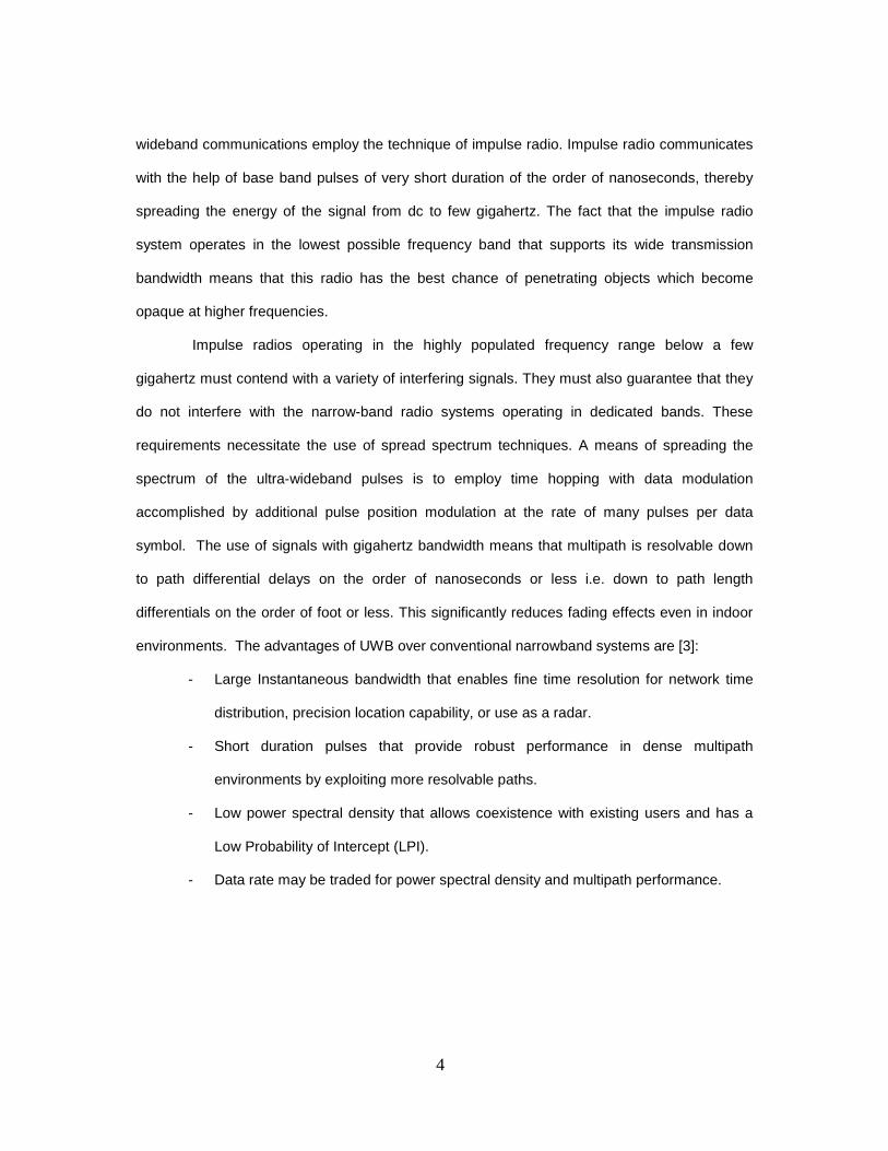
Figure 2.2. Gaussian pulse and Gaussian first derivative waveform [7].
Antennas on the transmitter and receiver act as differentiation operation on the signal,
meaning that the signal at the receiving end will be of higher derivative order than the generated
pulse. Thus the pulse after the transmitting antenna and in the channel will be of the 1st
derivative of a Gaussian pulse and the signal after the receiving antenna will be a 2nd derivative
of the Gaussian pulse [8]. Figure 2.2 shows Gaussian pulse and Gaussian first derivative
waveform.
2.3 FCC Regulations on UWB Technology
The FCC regulations classify UWB applications into several categories (Table 2.1) with
different emission regulations in each case. Maximum emissions in the prescribed bands are at
an effective isotropic radiated power (EIRP) of −41.3 dBm per MHz, and the −10 dB level of the
emissions must fall within the prescribed band (Figure 2.3) [9]. UWB emissions could potentially
interfere with other wireless communication system such as GPS, as well as other systems
using narrow band. Many factors such as, distance between devices, modulation technique and
propagation loss in a channel affects how UWB interferes with other narrow band devices. To
prevent UWB devices from causing harmful interferences to other devices, FCC came up with
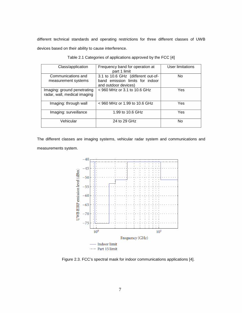
7
different technical standards and operating restrictions for three different classes of UWB
devices based on their ability to cause interference.
Table 2.1 Categories of applications approved by the FCC [4]
Class/application Frequency band for operation at part 1 limit
User limitations
Communications and measurement systems
3.1 to 10.6 GHz (different out-of-band emission limits for indoor and outdoor devices)
No
Imaging: ground penetrating radar, wall, medical imaging
< 960 MHz or 3.1 to 10.6 GHz Yes
Imaging: through wall < 960 MHz or 1.99 to 10.6 GHz Yes
Imaging: surveillance 1.99 to 10.6 GHz Yes
Vehicular 24 to 29 GHz No
The different classes are imaging systems, vehicular radar system and communications and
measurements system.
Figure 2.3. FCC’s spectral mask for indoor communications applications [4].
8
CHAPTER 3
ULTRA-WIDEBAND RADAR SYSTEMS
3.1 Salient Features of Ultra-wideband Radars
3.1.1. Precision Ranging
Timing of the pulse measures range, just as in conventional radar. As in conventional
radar, range resolution is given by
∆Range � c2. BW � τ. c2
Where c is the speed of electromagnetic wave
BW is the bandwidth of the pulse
6 is the width of the pulse in time domain
The large fractional bandwidth of UWB results in very short duration pulses in time domain. The
pulse duration is usually in the range of nanoseconds to a few tens of picoseconds. The short
pulse duration provides for very high range resolution and precision positioning capabilities.
3.1.2. Jamming and Detection resistance
UWB signal is noise-like due to the low energy density and the pseudo-random
characteristics of the transmitted signal. Hence, detection is difficult. Random noise waveform is
inherently low probability of intercept (LPI) and low probability of detection (LPD). Due to low
power, UWB signals do not cause significant interference to existing radio systems. The large
bandwidth along with discontinuous transmission makes UWB signal resistant to severe multi-
path interference and jamming. Thus, it is an ideal candidate sensor for covert imaging of
obscured regions in hostile environments [10, 11].
9
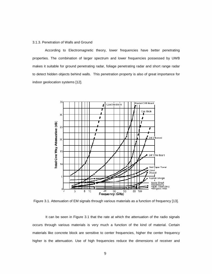
3.1.3. Penetration of Walls and Ground
According to Electromagnetic theory, lower frequencies have better penetrating
properties. The combination of larger spectrum and lower frequencies possessed by UWB
makes it suitable for ground penetrating radar, foliage penetrating radar and short range radar
to detect hidden objects behind walls. This penetration property is also of great importance for
indoor geolocation systems [12].
Figure 3.1. Attenuation of EM signals through various materials as a function of frequency [13].
It can be seen in Figure 3.1 that the rate at which the attenuation of the radio signals
occurs through various materials is very much a function of the kind of material. Certain
materials like concrete block are sensitive to center frequencies, higher the center frequency
higher is the attenuation. Use of high frequencies reduce the dimensions of receiver and

10
transmitter antennas but reduces the penetrating capability whereas use of lower frequencies
enhances the penetration capability of EM waves through the wall but can reduce the Radar
Cross Section (RCS) of the target when wavelength exceeds the size of the target. The FCC
regulations for through wall imaging are less than 960 MHz or 1.99 to 10.6 GHz which satisfies
both the requirement.
3.2 UWB Radar Fundamentals
A basic principle of the UWB radar is shown in Fig. 3.2. UWB radar generates and
transmits short pulse through the transmit antenna TX. The signal propagates in an
environment. When it meets target, the part of the electromagnetic energy is reflected from the
object and propagates back to receive antenna RX. The time delay between the transmitted and
received signal represents spatial distance between TX - target - RX.
Figure 3.2. Basic principle of the UWB radar [14].
For this thesis, Time Domain Corporation manufactured UWB radar “PulsON 220” was
used. This works on TM-UWB (Time modulated UWB) architecture also known as Impulse
Radio. The working on “PulsON 220” and TM-UWB radar are explained in the subsequent
sections. The setup for experimentation is discussed in the next chapter.
3.2.1. Block Diagram of TM-UWB Transceiver
Figure 3.3 shows high-level block diagram of a TM-UWB transceiver [10]. It can be
seen that a pulse generator generates the transmission pulse at required power and the
transmitter does not contain power amplifier. A vital part of the pulse generation circuit is the
antenna, which acts as a filter [10]. The architecture of receiver resembles the transmitter,
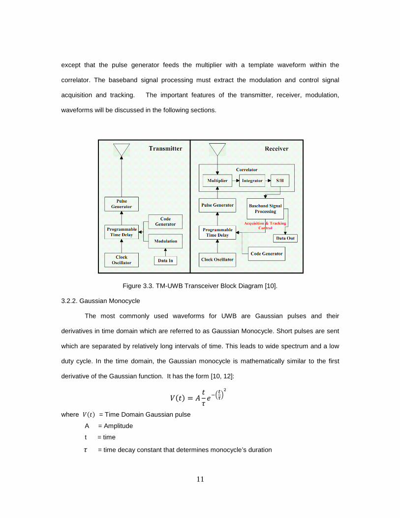
11
except that the pulse generator feeds the multiplier with a template waveform within the
correlator. The baseband signal processing must extract the modulation and control signal
acquisition and tracking. The important features of the transmitter, receiver, modulation,
waveforms will be discussed in the following sections.
Figure 3.3. TM-UWB Transceiver Block Diagram [10].
3.2.2. Gaussian Monocycle
The most commonly used waveforms for UWB are Gaussian pulses and their
derivatives in time domain which are referred to as Gaussian Monocycle. Short pulses are sent
which are separated by relatively long intervals of time. This leads to wide spectrum and a low
duty cycle. In the time domain, the Gaussian monocycle is mathematically similar to the first
derivative of the Gaussian function. It has the form [10, 12]:
7��� � 8 �6 ���9:#$ where 7��� = Time Domain Gaussian pulse
A = Amplitude
t = time 6 = time decay constant that determines monocycle’s duration

12
In the frequency domain, a Gaussian monocycle’s spectrum is of the form:
7��� � ;< � 6( ���=:�$
Where 7��� is the Gaussian pulse frequency domain response
The center frequency is then proportional to the inverse of the pulse duration, i.e.:
� > 16
The most basic element of Time Domain's TM-UWB radio technology is based on
implementation of a Gaussian monocycle. Figure 3.4 shows an idealized monocycle in time
and frequency domains [10].
Figure 3.4. Gaussian Monocycle in Time domain and Frequency domain [10].
The center frequency of a monocycle is the reciprocal of the monocycle's duration and
the bandwidth is 116% of the monocycle’s center frequency. Thus, for the 0.5-ns monocycle
shown in Figure 3.4, the center frequency is 2 GHz and the half power bandwidth is
approximately 2GHz.
In PulsON 220, first order Gaussian monopulse is employed for short pulse
transmissions. The transmitting antenna has the general effect of differentiating the time
waveform presented to it. As a result of this the transmitted pulse does not have a DC value -
the integral of the waveform over its duration must equal zero. Figure 3.5 shows the effects of

13
antenna on a UWB pulse. The received signals are second order derivate of Gaussian
monopulse.
Figure 3.5. Effect of antennas on UWB pulse [15].
3.2.3. UWB Transmitter
TM-UWB transmitters emit very short duration Gaussian monocycles with tightly
controlled pulse-to-pulse intervals. The pulse-to-pulse intervals are relatively long. Thus, the
short duration pulse leads to wide band signal and long pulse-to-pulse interval leads to low duty
cycle. Time Domain UWB products have monocycle pulse widths of between 0.20 and 1.50
nanoseconds and pulse-to-pulse intervals of between 25 and 1000 nanoseconds [10, 12]. Pulse
position modulation (PPM) scheme is used in the systems and pulse-to-pulse interval is varied
on a pulse-by-pulse basis in accordance with two components: an information signal and a
channel code. A single bit of information is transmitted using multiple pulses.

14
3.2.4. Monocycle Sequence
The PulsON systems use long sequences of monocycles for communications instead of
single monocycles. Based on the information signal and channel code, PPM is used to vary the
pulse-to-pulse intervals. When the sequences of monocycles are sent, it is important to ensure
the spectral quality integrity. Figure 3.6 contains an illustration of a Gaussian monocycle
sequence. In the frequency domain, this highly regular monocycle pulse train produces energy
spikes at regular intervals [10]. This results in the already low power signal to spread among the
comb lines. This monocycle pulse train carries no information. Because of the regularity of the
energy spikes, it may interfere with conventional radio systems at very short ranges.
Figure 3.6. A periodic pulse train in Time and Frequency domain [10, 12].
The comb lines can be eliminated by varying the pulse-to-pulse intervals. Data
modulation and channelization are employed to vary the pulse-to-pulse intervals which eliminate
the spikes. This also gives it noise-like characteristics.
3.2.5. Modulation
To transmit information, additional processing is needed to modulate the monocycle
pulse train. The modulation scheme used in PulsON 220 is FLIP modulation. In this scheme,
pulse polarity is varied in combination with the pulse position modulation which allows for 2 bits
per symbol. Figure 3.7 shows the FLIP modulation scheme. As shown in the figure 3.7, PPM
varies the precise timing of a monocycle transmission about the nominal position. For example,
in a 10 million pulses per second (Mpps) system, monocycles would be transmitted nominally
15
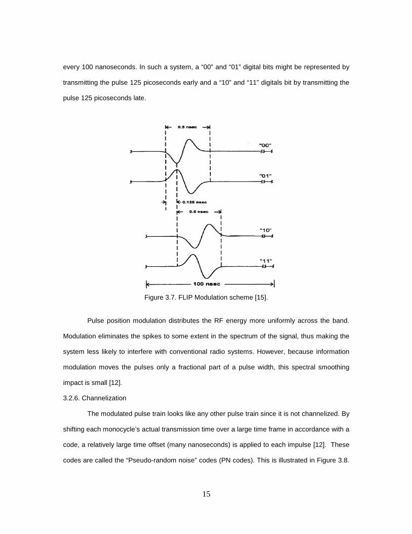
every 100 nanoseconds. In such a system, a “00” and “01” digital bits might be represented by
transmitting the pulse 125 picoseconds early and a “10” and “11” digitals bit by transmitting the
pulse 125 picoseconds late.
Figure 3.7. FLIP Modulation scheme [15].
Pulse position modulation distributes the RF energy more uniformly across the band.
Modulation eliminates the spikes to some extent in the spectrum of the signal, thus making the
system less likely to interfere with conventional radio systems. However, because information
modulation moves the pulses only a fractional part of a pulse width, this spectral smoothing
impact is small [12].
3.2.6. Channelization
The modulated pulse train looks like any other pulse train since it is not channelized. By
shifting each monocycle’s actual transmission time over a large time frame in accordance with a
code, a relatively large time offset (many nanoseconds) is applied to each impulse [12]. These
codes are called the “Pseudo-random noise” codes (PN codes). This is illustrated in Figure 3.8.
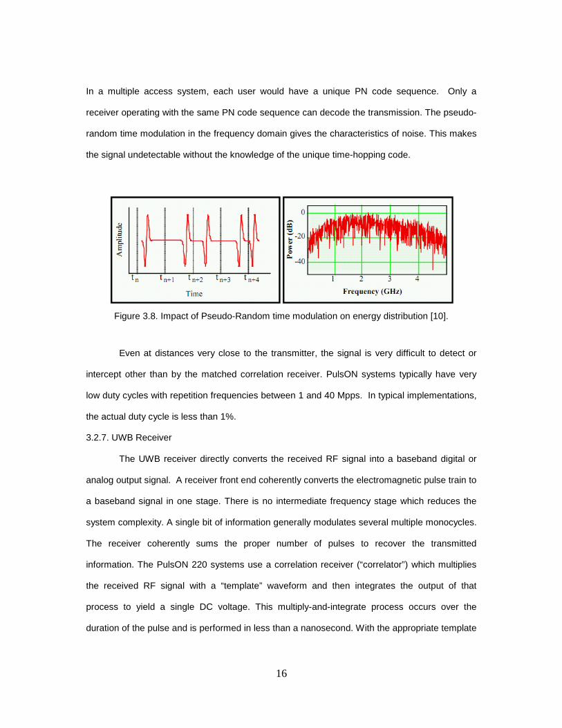
16
In a multiple access system, each user would have a unique PN code sequence. Only a
receiver operating with the same PN code sequence can decode the transmission. The pseudo-
random time modulation in the frequency domain gives the characteristics of noise. This makes
the signal undetectable without the knowledge of the unique time-hopping code.
Figure 3.8. Impact of Pseudo-Random time modulation on energy distribution [10].
Even at distances very close to the transmitter, the signal is very difficult to detect or
intercept other than by the matched correlation receiver. PulsON systems typically have very
low duty cycles with repetition frequencies between 1 and 40 Mpps. In typical implementations,
the actual duty cycle is less than 1%.
3.2.7. UWB Receiver
The UWB receiver directly converts the received RF signal into a baseband digital or
analog output signal. A receiver front end coherently converts the electromagnetic pulse train to
a baseband signal in one stage. There is no intermediate frequency stage which reduces the
system complexity. A single bit of information generally modulates several multiple monocycles.
The receiver coherently sums the proper number of pulses to recover the transmitted
information. The PulsON 220 systems use a correlation receiver (“correlator”) which multiplies
the received RF signal with a “template” waveform and then integrates the output of that
process to yield a single DC voltage. This multiply-and-integrate process occurs over the
duration of the pulse and is performed in less than a nanosecond. With the appropriate template

17
waveform, the output of the correlator is a measure of the relative time positions and the polarity
of the received monocycle and the template. Figure 3.9 shows the output of the correlator that
corresponds to different time offsets between the template and the received waveform. When a
monocycle is hidden in the noise of other signals, it is impossible to detect the reception of a
single UWB pulse. Pulse integration is performed by the addition of numerous correlator
samples to receive the transmitted signals. Through pulse integration PulsON receivers can
acquire, track and demodulate UWB transmissions that are significantly below noise floor [12].
Figure 3.9. Correlator receiver with template [15].
The measure of an UWB receiver’s performance in presence of in-band noise signals is
processing gain. This is described in the next section.
18
3.2.8. Processing Gain and Interference Resistance
The time-modulated UWB radios are built based on the concepts of pseudo-random
coding, random time modulation and correlation receivers. This results in UWB radars being
highly resistant to interference. This is critical as all other signals within the band occupied by a
time-modulated signal act as jammers. Since there are no unallocated multiple GigaHertz bands
available for time-modulated systems, the UWB systems always encounter interference from
other systems. Processing gain provides a measure of a radio’s resistance to jamming.
Processing gain is defined as the ratio of the signal’s RF bandwidth to the information
bandwidth of the signal. Time-modulated UWB radios have a huge processing gain. For a
PulsON signal, the processing gain may be calculated from: the duty cycle of the transmission,
e.g., a 1% duty cycle yields a process gain of 20 dB. The effect of pulse integration, e.g.,
integrating energy over 100 pulses to determine one digital bit yields a process gain of 20 dB.
The total process gain is then the sum of these two components, e.g., 40 dB. For example, a 2-
GHz / 10-Mpps link transmitting 8 kbps would have a process gain of 54 dB, because it has a
0.5-ns pulse width with a 100-ns pulse repetition interval = 0.5% duty cycle (23 dB) and 10
Mpps / 8,000 bps = 1250 pulses per bit (another 31 dB) [12].
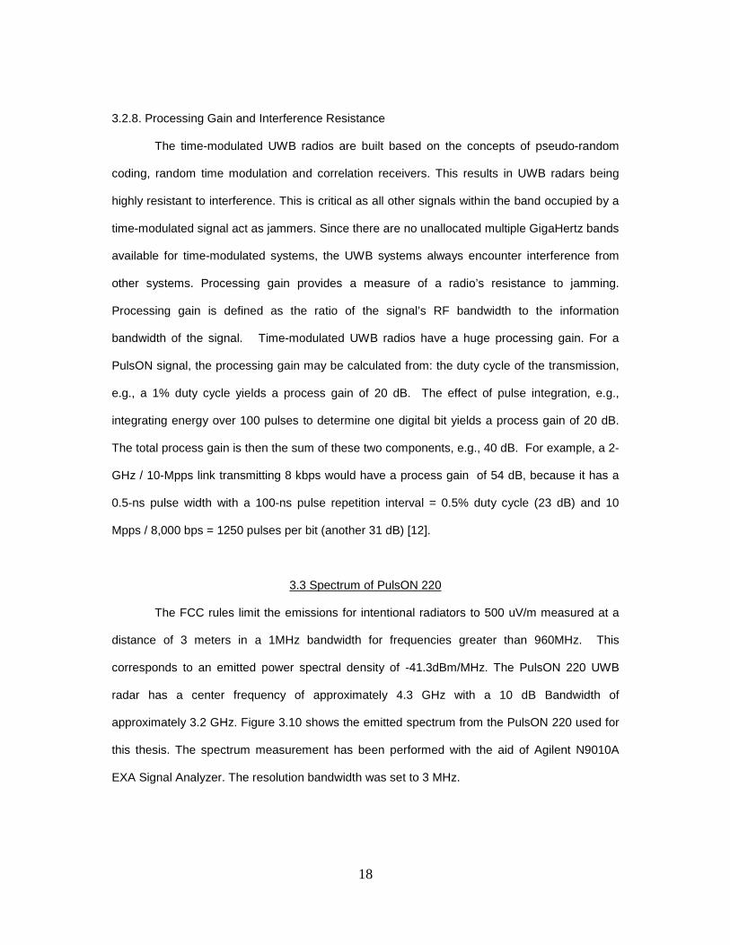
3.3 Spectrum of PulsON 220
The FCC rules limit the emissions for intentional radiators to 500 uV/m measured at a
distance of 3 meters in a 1MHz bandwidth for frequencies greater than 960MHz. This
corresponds to an emitted power spectral density of -41.3dBm/MHz. The PulsON 220 UWB
radar has a center frequency of approximately 4.3 GHz with a 10 dB Bandwidth of
approximately 3.2 GHz. Figure 3.10 shows the emitted spectrum from the PulsON 220 used for
this thesis. The spectrum measurement has been performed with the aid of Agilent N9010A
EXA Signal Analyzer. The resolution bandwidth was set to 3 MHz.
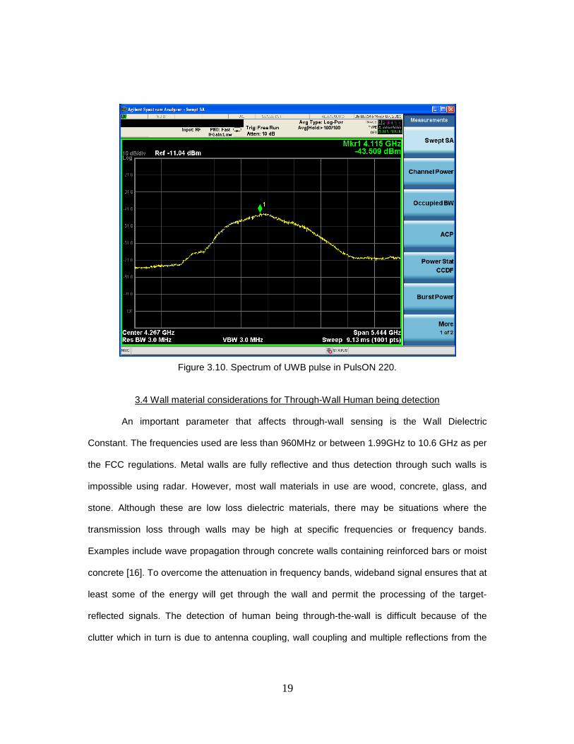
Figure 3.
3.4 Wall material considerations
An important parameter that affects through
Constant. The frequencies used are less than 960MHz or between
the FCC regulations. Metal walls are
impossible using radar. However,
stone. Although these are low loss
transmission loss through wall
Examples include wave propagation
concrete [16]. To overcome the attenuation in frequency bands, wideband signal ensures that
least some of the energy will get through the wall and permit the
reflected signals. The detection of human being through
clutter which in turn is due to antenna coupling, wall coupling and multiple refle
19
.10. Spectrum of UWB pulse in PulsON 220.
Wall material considerations for Through-Wall Human being detection
An important parameter that affects through-wall sensing is the Wall Dielectric
Constant. The frequencies used are less than 960MHz or between 1.99GHz to 10.6 GHz
Metal walls are fully reflective and thus detection through such walls is
impossible using radar. However, most wall materials in use are wood, concrete, glass, and
stone. Although these are low loss dielectric materials, there may be situations where the
transmission loss through walls may be high at specific frequencies or frequency bands.
Examples include wave propagation through concrete walls containing reinforced bars or moist
To overcome the attenuation in frequency bands, wideband signal ensures that
of the energy will get through the wall and permit the processing of the target
The detection of human being through-the-wall is difficult because of the
clutter which in turn is due to antenna coupling, wall coupling and multiple reflections from the
Human being detection
wall sensing is the Wall Dielectric
to 10.6 GHz as per
ve and thus detection through such walls is
most wall materials in use are wood, concrete, glass, and
dielectric materials, there may be situations where the
be high at specific frequencies or frequency bands.
through concrete walls containing reinforced bars or moist
To overcome the attenuation in frequency bands, wideband signal ensures that at
processing of the target-
wall is difficult because of the
ctions from the
20
wall. A signal transmitted through the antenna suffers attenuation due to the wall and other
obstacles around. Figure 3.11 shows multiple reflections of the signal from the boundaries of
the wall.
Figure 3.11. Signal Reflection from Wall [14].
The transmission of electromagnetic waves through the wall causes decrease in
velocity due to the dielectric constant of the wall. Higher the dielectric constant and more the
thickness of the wall larger will be the delay. This results in the targets behind the wall to appear
farther away than they actually are [17].
3.5 Human Being Detection
Detection of human beings with radars is based on movement detection. Heart beat
and respiratory motions cause changes in frequency, phase, amplitude and arrival time of
reflected signal from a human being [2]. These changes are extremely small for through-wall
detection and different techniques should be devised to extract these minute variations.
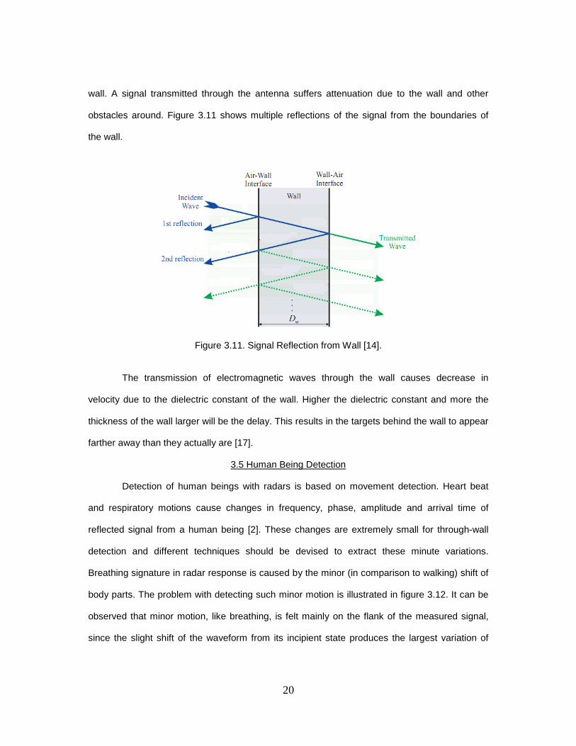
Breathing signature in radar response is caused by the minor (in comparison to walking) shift of
body parts. The problem with detecting such minor motion is illustrated in figure 3.12. It can be
observed that minor motion, like breathing, is felt mainly on the flank of the measured signal,
since the slight shift of the waveform from its incipient state produces the largest variation of
21
waveform at the steepest slope [1]. Some important features needed to be considered during
the detection process are:
- The range resolution of the radar should be more than the geometrical variations of the
chest caused by breathing.
- Breathing is a periodical motion over a certain interval of time. The frequency of
breathing can change slowly with the time, but it is always within the frequency window,
(0.2—0.5 Hz).
- The response from breathing person is extremely weak due to the wall materials which
attenuate the electromagnetic waves.
Figure 3.12. Principle of detecting minor motions by means of UWB radar [1].
- Reflected UWB signal is highly sensitive to human posture which makes detection
process challenging.
22
CHAPTER 4
EQUIPMENT CONFIGURATIONS AND MEASUREMENTS
The hardware used for Through-Wall human detection is PulsON 220. PulsON products
have been developed by Time Domain Corporation based on Time modulated Ultra Wideband
(TM-UWB) architecture. The usage of PulsON radar in monostatic mode has been explained in
this chapter and also some important terms associated with it. The waveform pulses are
transmitted from a single Omni-directional antenna and the scattered waveforms are received
by a collocated Omni-directional antenna. The two antenna ports on the P220 are used for
transmit and receive antennas.
4.1 PulsON 220 in Monostatic mode
Monostatic radar (MSR) consists of two components: an embedded side and a host
side. The embedded component runs on the radio; it interfaces with the host computer via
Ethernet and controls the radio using the UWB Kernel. The host side runs on a PC; it sends
commands to and receives status info and radar scans from the embedded component via
Ethernet. The basic procedure to setup P220 in monostatic mode is described in detail in [18].
Only the important parameters are discussed here. In this mode we use two Omni-directional
antennas connected to ports A and B of the radio. An Ethernet cable is used to connect the
radio to the PC and radar can be controlled using GUI PulsON 220 MSR 1.1 application
software provided with the radios. An IP address is assigned to the radar and another to PC and
we can establish IP link using the GUI. Figure 4.1 below shows the P220 in Monostatic mode.

23
Figure 4.1. P220 in Monostatic mode
4.1.1. Radio Configuration
The important tabs and parameters associated with the PulsON 220 MSR 1.1 GUI are
described in this section.
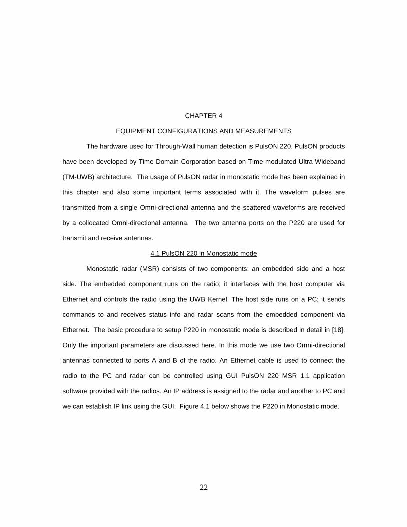
4.1.1.1 Setup tab
The important parameters in the Setup tab are pulse integration, pulse repetition
frequency and code file. Figure 4.2 shows the default parameters in the Setup tab.
Integration is the number of radio pulses combined to increase the signal-to-noise ratio.
There are two types of integration. Hardware integration is performed by the radio’s
hardware/firmware. Software integration is performed by the radio’s kernel software and occurs
after hardware integration. The total integration is the total number of UWB pulses per
waveform sample, and is found by multiplying hardware by software integration [18]. The default
values for Hardware and Software Integration are 512 and 2 respectively.
Pulse repetition frequency is the rate at which radio transmits UWB pulses. The highest
supported rate which is also the default value is 9.6 MHz. A slower pulse rate results in slower
scans, but increases the radar’s unambiguous range. At 9.6 MHz, the maximum unambiguous
range (distance where a pulse sent / returned and the next pulse sent do not overlap) is
24
approximately 50 ft. The range increases to 100 ft. at 4.8 MHz, 200 ft. at 2.4 MHz, and 400 ft.
at 1.2 MHz [18].
Codefile is the time-hopping (time-dither) code file on the radio used to reduce noise
and spread the UWB signal’s spectrum [18].
Figure 4.2. MSR analysis tool - Setup tab [19].
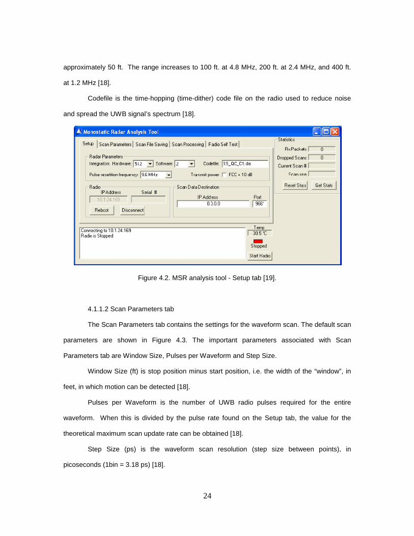
4.1.1.2 Scan Parameters tab
The Scan Parameters tab contains the settings for the waveform scan. The default scan
parameters are shown in Figure 4.3. The important parameters associated with Scan
Parameters tab are Window Size, Pulses per Waveform and Step Size.
Window Size (ft) is stop position minus start position, i.e. the width of the “window”, in
feet, in which motion can be detected [18].
Pulses per Waveform is the number of UWB radio pulses required for the entire
waveform. When this is divided by the pulse rate found on the Setup tab, the value for the
theoretical maximum scan update rate can be obtained [18].
Step Size (ps) is the waveform scan resolution (step size between points), in
picoseconds (1bin = 3.18 ps) [18].
25
Figure 4.3. MSR analysis tool – Scan Parameters tab [18].
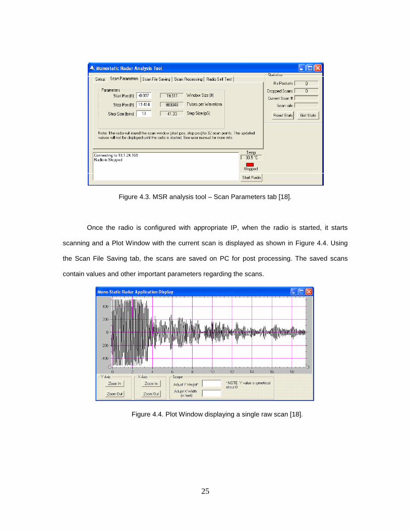
Once the radio is configured with appropriate IP, when the radio is started, it starts
scanning and a Plot Window with the current scan is displayed as shown in Figure 4.4. Using
the Scan File Saving tab, the scans are saved on PC for post processing. The saved scans
contain values and other important parameters regarding the scans.
Figure 4.4. Plot Window displaying a single raw scan [18].

26
4.2 PulsOn220 Specifications
The important specifications for PulsON 220 have been mentioned in the tables 4.1 and
4.2. Table 4.1 shows the center frequency, bandwidth, EIRP and the pulse duration. Table 4.2
shows the maximum unambiguous range for a given Raw Data rate under free space and
residential/office environment.
Table 4.1 Specifications of the PulsON 220 radio [19]
Parameter
UWB ( PulsON 220)
Center Freq.
Approx. 4.27 GHz
10dB - Bandwidth
3.2 GHz
Pulse type
1st order Gaussian Monocycle – [10,19]
Pulse Duration
430 ps
Pulse Length
0.13 m
Resolution
6.5 cm
Power Consumption
5.7 Watts
EIRP -12.8 dBm
Table 4.2 Data based on standard FCC 15.517 power [10]
Raw Data Rate Free Space Average Range
of Operation Residential / Office Average
Range of Operation 9.6 Mbps 17-20 meters 6.4-7.4 meters 2.4 Mbps 35-40 meters 10-12 meters 600 kbps 70-80 meters 16-19 meters 150 kbps 130-160 meters 25-30 meters
27
4.3 Data Collection
While collecting the data, the scans were acquired for duration of 60-80seconds. The
Waveform scan resolution, window size, pulse repetition frequency and the pulse integration
defines the scan rate which is basically the number of scans acquired per minute. The
equations below show the relation between some important parameters associated with the
scans:
@A�BCD EAF� ������ � E�CG HCIA�AC��A� ����� ; E�J�� HCIA�AC��A� �����
KLM�� C� NJ�J HCA��I G�� EJ� � EJ�E�CGOA� ; EJ�E�J��OA� E��G EAF��MA�I�
EJ�E�CGOA������� ; EJ�E�J��OA������� � 2 P @A�BCD EAF������� P 0.3048
Where c = 3 * 108 m/s is the speed of EM Waves
Twice the Window size indicates the distance to reach the target and return to the
receiver.
1 OA� � 3.18GI
KLM�� C� NJ�J HCA��I G�� EJ� � 2 P @A�BCD EAF������� P 0.3048 P E��G EAF��A� I�C�BI�
KC. C� HUI�I G�� EJ� � V@ A�� P E@ W�� P KC. C� NJ�J HCA��I G�� IJ� EJ� XAL� � KLM�� C� HUI�I G�� EJ�HUI� Y�G��A�AC� �������
EJ� YJ�� � 1EJ� XAL�
XC�JU �LM�� C� EJ�I CUU���B � EJ� YJ�� P XC�JU BJ�J CUU��AC� �AL�

28
The above expressions indicate that increasing the scan Window Size or Integration
size increases the scan time and thus reduces the Scan Rate. However increasing the Step
Size increases the Scan Rate. The least Step Size that can be set is 1 bin. Setting the Step size
to 1 bin reduces the scan rate but minute variations are captured whereas increasing the Step
size increases the scan rate but minute variations are not captured accurately. Decreasing the
Pulse repetition frequency increases the unambiguous range and thus reduces the scan rate.
4.4 Measurement Locations
The measurements were taken at three different locations having different types of
walls. First set of readings were taken for Gypsum wall, second set of readings were taken with
Wooden door being the obstacle and the third set of readings were taken for Concrete wall. At
every location, readings were taken with human being present (stationary and motionless) on
the other side of the obstacle and with no human target present. After acquiring the data, post
processing was done by employing three different algorithms which will be described in the next
chapter.
The radar parameters employed in each of the cases given below were
Integration: Hardware Integration = 512, Software Integration = 2
Hardware Integration = 512, Software Integration = 4
Pulse Repetition Frequency: 9.6 MHz
Step Size: 1 bin, 4 bin, 7 bin, 13 bin
Window Size: 9 feet
4.4.1. Gypsum Wall (Nedderman Hall Room 202 & 203)
Figure 4.5 shows the schematic diagram of location of the radar and Human target on
different sides of a 1’1” thick Gypsum partition wall. Human target is at a distance of 3.5ft from
the radar on the other side of the wall. The height of the antennas from ground is 3’4”. The
details related to room dimensions and objects in the room can be found in the Figure 4.5. The

29
left image of Figure 4.6 shows the human target located in NH 203 and the right image shows
the UWB radar located in NH 202. The two rooms are separated by 1’1” Gypsum wall. Gypsum
partition walls usually have gypsum boards on each side with fiber glass insulation inside.
Figure 4.5. Location of Radar and Human Target, Partition wall – Gypsum Wall.
Figure 4.6. Human Target in NH 203 (left image), UWB Radar in NH 202(right).

30
4.4.2. Wooden door (Nedderman Hall 205)
The figure 4.7 below shows the schematic diagram of location of the radar and Human
target on different sides of a 4” wooden door. Human target is standing at a distance of 5.5ft
from the radar on the other side of the door and the height of the antennas from ground is 3’4’’.
The details related to room dimensions and objects in the room can be found in the Figure 4.7.
Figure 4.8 shows the image with UWB radar being in NH 201 and Human standing outside.
Figure 4.7. Wooden door, Location of Radar and Human Target.
Figure 4.8. UWB Radar in NH 201 and Human target standing outside.

31
4.4.3. Load Bearing Concrete wall (NH 2nd Floor, Near Elevators)
The figure 4.9 below shows the schematic diagram of location of the radar and Human
target on different sides of a 1’1” thick Concrete Wall. Human target is standing at a distance of
4 ft from the radar on the other side of the concrete wall and the height of the antennas from
ground is 3’4’’. The details related to dimensions and objects on the floor can be found in the
Figure 4.9.
Figure 4.9. Concrete wall, Location of Radar and Human Target.
32
CHAPTER 5
RESULTS AND ANALYSIS
The algorithms used for human target detection through-the-wall have been described
in this chapter. The results associated with each algorithm and for each wall type have been
provided. Even though measurements were taken for different step sizes viz. 1 bin, 4 bin, 7 bin
and 13 bin; the analysis was done on 1 bin step size only since minute variations could be
captured with it. The Hardware Integration used was 512 pulses and software integration used
was 2. The approaches presented are based on detection of respiratory motion. The process of
inhaling and exhaling leads to small chest movements which is periodic in nature. This motion is
very small and results in very weak radar echo. But since it is periodic motion it can be detected
by application of signal processing techniques which enhances the “breathing” signal from
noise.
5.1 Detection using Normalized Difference Square Technique
The scans obtained using PulsON 220 UWB radar is used to create M x N matrix
where ‘N’ is the number of scans and ‘M is the number of samples per scan. The difference
between successive scans are taken which captures changes from one scan to another and
helps to suppress the static clutter in the signal. This is indicated by the DIFFMATRIX. By
taking the square of each difference, the scans where inhalation and exhalation occur are
enhanced. This is represented by DIFFSQUARE matrix. Normalization is done by dividing each
value in the DIFFSQUARE matrix by highest value in DIFFSQUARE matrix. When this matrix is
constructed and contour plotting is done using Matlab, human target at a distance slightly more
than the actual distance can be clearly seen. The increase in distance is due to the fact that the

33
electromagnetic waves should pass the wall which has a different dielectric constant then air
and hence the speed of EM waves reduces. The approach is as follows:
Step 1: SCANMAT Matrix is constructed using ‘N’ scans arranged in columns. In Scan(i,j), i
indicates Scan number and j indicates Sample number corresponding to the scan
SCANMAT � ` Scan�1,1� Scan�2,1� Scan�3,1�Scan�1,2� Scan�2,2� Scan�3,2� bb Scan�N, 1�Scan�N, 2�c c c d c Scan�1, M� Scan�2, M� Scan�3, M� b Scan�N, M�e
Step 2: DIFFMATRIX is the difference between successive columns of SCANMAT.
ScanDiff(i,j) = Scan(i, j) – Scan(i+1,j)
DIFFMATRIX � ` ScanDiff�1,1� ScanDiff�2,1� ScanDiff�3,1�ScanDiff�1,2� ScanDiff�2,2� ScanDiff�3,2� bb ScanDiff�N ; 1,1�ScanDiff�N ; 1,2�c c c d c ScanDiff�1, M� ScanDiff�2, M� ScanDiff�3, M� b ScanDiff�N ; 1, M�e
Step 3: Construct DIFFSQUARE matrix and normalize it.
SqDi(i,j) = (ScanDiff(i,j))2
DIFFSQUARE � ` SqDi�1,1� SqDi�2,1� SqDi�3,1�SqDi�1,2� SqDi�2,2� SqDi�3,2� bb SqDi�N ; 1,1�SqDi�N ; 1,2�c c c d c SqDi�1, M� SqDi�2, M� SqDi�3, M� b SqDi�N ; 1, M�e
Step 4: The normalized matrix is M x (N-1) matrix. Use contour mapping feature from Matlab
with x-axis being time in seconds and y-axis being distance from the UWB radar.
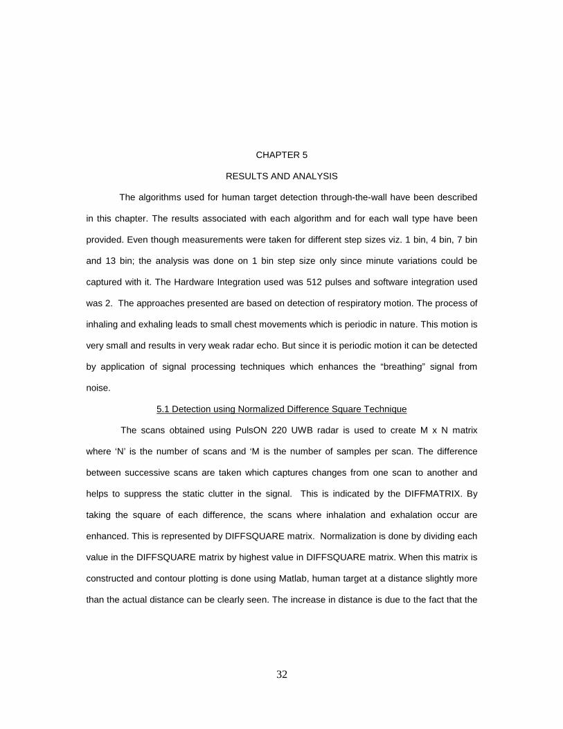
5.1.1. Gypsum Wall
Figure 5.1 shows a single scan taken for a Gypsum wall with target, without target and
difference between the two scans. In this case the human target is at 3.5ft from the radar.
Figure 5.2 and Figure 5.3 shows the plot using Normalized Square of Difference of successive
scans method for cases with Human target and No target respectively. In Figure 5.2, the
presence of human target at a distance of approximately 3.5 – 4 feet can be clearly seen.
34
Figure 5.1. Gypsum Wall, single scan with target, No Target and difference.
Figure 5.2. Gypsum Wall, Normalized Square of Difference of scans with Target.
0 1 2 3 4 5 6 7 8 9-1000
0
1000Single Scan with Target at 3.5ft
0 1 2 3 4 5 6 7 8 9-1000
0
1000Single Scan with No Target
0 1 2 3 4 5 6 7 8 9-1000
0
1000Single Scan with Hand Movement
0 1 2 3 4 5 6 7 8 9-500
0
500Difference of Single Scan between Target and No Target
0 1 2 3 4 5 6 7 8 9-500
0
500Difference of Single Scan between Target with Hand Movement and No Target
Distance in feet from UWB Radar
Time is seconds
Dis
tanc
e in
fee
t
Normalised Difference Square Matrix with Target at 3.5 feet
5 10 15 20 25 30 35 40
1
2
3
4
5
6
7
8
9
1
2
3
4
5
6
7
8
9
10
35
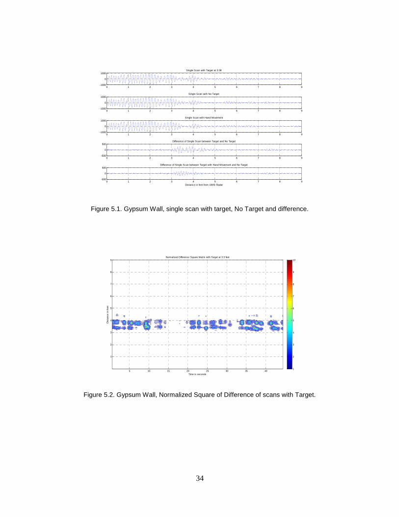
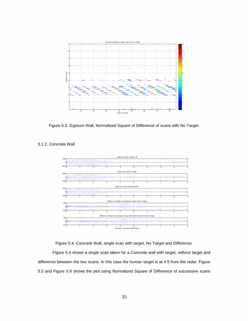
Figure 5.3. Gypsum Wall, Normalized Square of Difference of scans with No Target.
5.1.2. Concrete Wall
Figure 5.4. Concrete Wall, single scan with target, No Target and Difference.
Figure 5.4 shows a single scan taken for a Concrete wall with target, without target and
difference between the two scans. In this case the human target is at 4 ft from the radar. Figure
5.5 and Figure 5.6 shows the plot using Normalized Square of Difference of successive scans
Time in seconds
Dis
tanc
e in
fee
t
Normalized Difference Square matrix with No Target
10 20 30 40 50 60 70 80
1
2
3
4
5
6
7
8
9
1
2
3
4
5
6
7
8
9
10
0 1 2 3 4 5 6 7 8 9-1000
0
1000Single Scan with Target at 4ft
0 1 2 3 4 5 6 7 8 9-1000
0
1000Single Scan with No Target
0 1 2 3 4 5 6 7 8 9-1000
0
1000Single Scan with Hand Movement
0 1 2 3 4 5 6 7 8 9-100
0
100Difference of Single Scan between Target and No Target
0 1 2 3 4 5 6 7 8 9-100
0
100Difference of Single Scan between Target with Hand Movement and No Target
Distance in feet from UWB Radar

36
method for cases with Human target and No target respectively. In Figure 5.5, the presence of
human target at a distance of approximately 4 – 4.5 feet can be clearly seen.
Figure 5.5. Concrete Wall, Normalized Square of Difference of scans with Target.
Figure 5.6. Concrete Wall, Normalized Square of Difference of scans with No Target
Time in seconds
Dis
tanc
e in
fee
tNormalized Difference Square matrix with Target
5 10 15 20 25 30 35 40 45
1
2
3
4
5
6
7
8
9
1
2
3
4
5
6
7
8
9
10
Time in seconds
Dis
tanc
e in
fee
t
Normalized Difference Square matrix with No Target
5 10 15 20 25 30 35 40 45
1
2
3
4
5
6
7
8
9
1
2
3
4
5
6
7
8
9
10
37
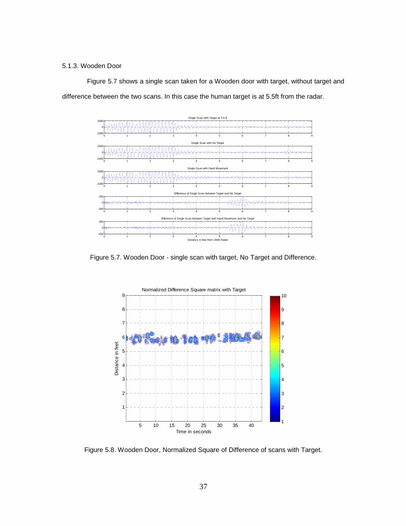
5.1.3. Wooden Door
Figure 5.7 shows a single scan taken for a Wooden door with target, without target and
difference between the two scans. In this case the human target is at 5.5ft from the radar.
Figure 5.7. Wooden Door - single scan with target, No Target and Difference.
Figure 5.8. Wooden Door, Normalized Square of Difference of scans with Target.
0 1 2 3 4 5 6 7 8 9-1000
0
1000Single Scan with Target at 5.5 ft
0 1 2 3 4 5 6 7 8 9-1000
0
1000Single Scan with No Target
0 1 2 3 4 5 6 7 8 9-1000
0
1000Single Scan with Hand Movement
0 1 2 3 4 5 6 7 8 9-200
0
200Difference of Single Scan between Target and No Target
0 1 2 3 4 5 6 7 8 9-200
0
200Difference of Single Scan between Target with Hand Movement and No Target
Distance in feet from UWB Radar
Time in seconds
Dis
tanc
e in
fee
t
Normalized Difference Square matrix with Target
5 10 15 20 25 30 35 40
1
2
3
4
5
6
7
8
9
1
2
3
4
5
6
7
8
9
10
38
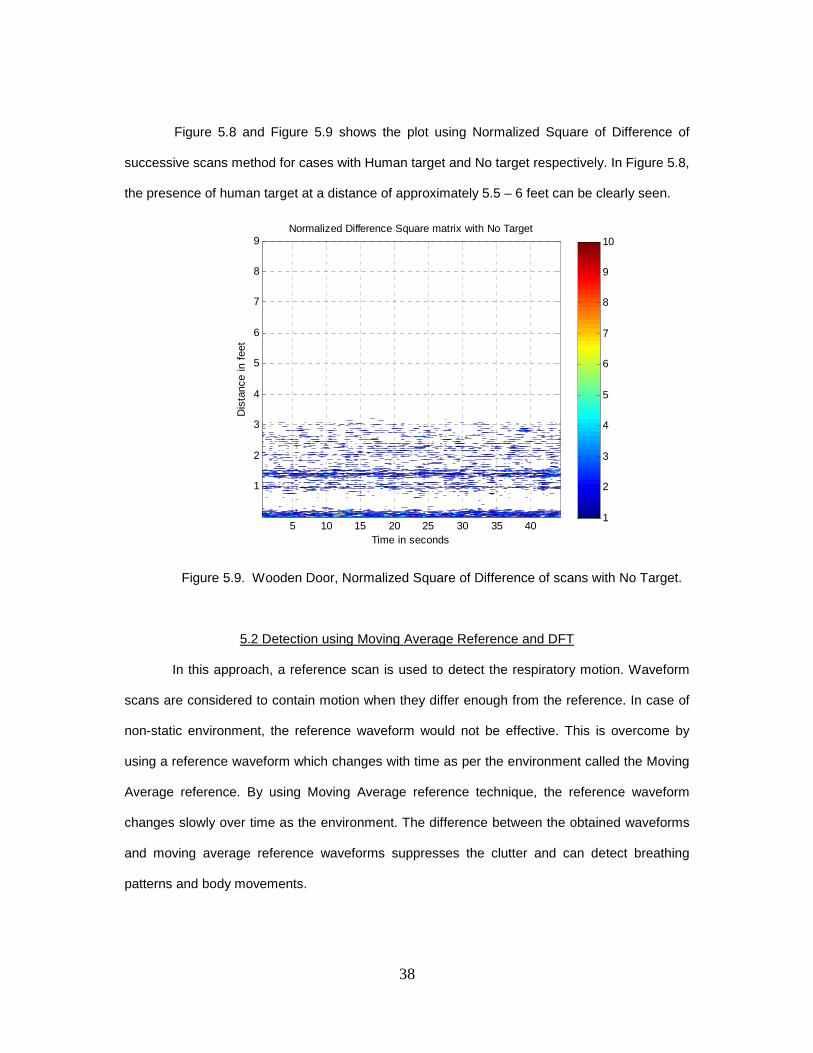
Figure 5.8 and Figure 5.9 shows the plot using Normalized Square of Difference of
successive scans method for cases with Human target and No target respectively. In Figure 5.8,
the presence of human target at a distance of approximately 5.5 – 6 feet can be clearly seen.
Figure 5.9. Wooden Door, Normalized Square of Difference of scans with No Target.
5.2 Detection using Moving Average Reference and DFT
In this approach, a reference scan is used to detect the respiratory motion. Waveform
scans are considered to contain motion when they differ enough from the reference. In case of
non-static environment, the reference waveform would not be effective. This is overcome by
using a reference waveform which changes with time as per the environment called the Moving
Average reference. By using Moving Average reference technique, the reference waveform
changes slowly over time as the environment. The difference between the obtained waveforms
and moving average reference waveforms suppresses the clutter and can detect breathing
patterns and body movements.
Time in seconds
Dis
tanc
e in
fee
tNormalized Difference Square matrix with No Target
5 10 15 20 25 30 35 40
1
2
3
4
5
6
7
8
9
1
2
3
4
5
6
7
8
9
10

39
The Moving average reference is given by an empirical formula:
pCqY���A, <� � 0.8569�Scan�A ; 3, <� � 0.0455uScan�A ; 2, <�v � 0.0476uScan�A ; 1, <�v� 0.05�Scan�A, <��
Where i >=4, i indicates present Scan number, i-1 indicates previous scan and so on.
j indicates sample number corresponding to the scan
When i is 2 or 3, MovRef(i,j) = Scan(i,j) – Scan(i-1,j)
When i is 1, MovRef(i,j) = Scan(i,j)
The scans obtained using PulsON 220 UWB radar is used to create M x N matrix called
the SCANMAT where ‘N’ is the number of scans and ‘M is the number of samples per scan.
Using the empirical formula for Moving reference, MOVREF matrix of M x N is constructed and
the difference between the two matrices called DIFFMAT is obtained. When this matrix is
constructed and contour plotting is done using Matlab, human target can be detected. The
approach is summarized below:
Step 1: SCANMAT Matrix is constructed using ‘N’ scans arranged in columns. In Scan(i,j), i
indicates Scan number and j indicates Sample number corresponding to the scan
SCANMAT � ` Scan�1,1� Scan�2,1� Scan�3,1�Scan�1,2� Scan�2,2� Scan�3,2� bb Scan�N, 1�Scan�N, 2�c c c d c Scan�1, M� Scan�2, M� Scan�3, M� b Scan�N, M�e
Step 2: MOVREF is the constructed using the empirical formula for the same
MOVREF � ` MovRef�1,1� MovRef�2,1� MovRef�3,1�MovRef�1,2� MovRef�2,2� MovRef�3,2� bb MovRef�N, 1�MovRef�N, 2�c c c d c MovRef�1, M� MovRef�2, M� MovRef�3, M� b MovRef�N, M�e
Step 3: DIFFMAT is obtained by taking the difference of SCANMAT and MOVREF
DIFFMAT � SCANMAT ; MOVREF Use contour mapping feature from Matlab with x-axis being time in seconds and y-axis being
distance from the UWB radar.
40
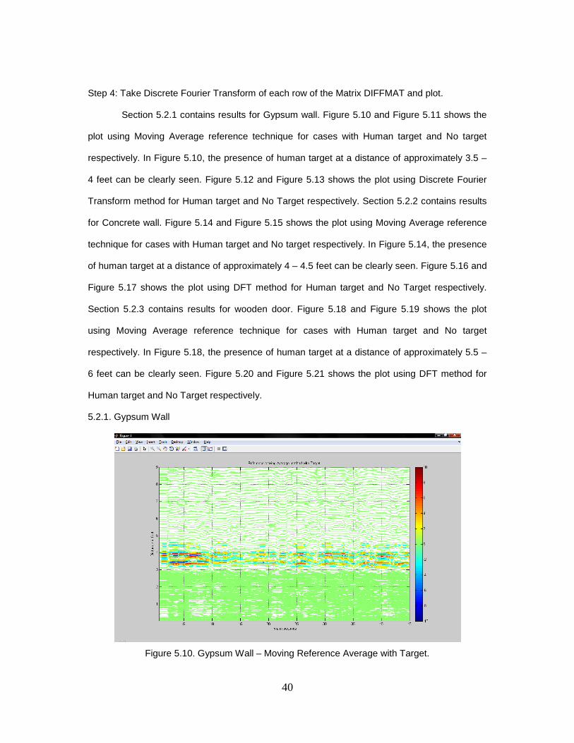
Step 4: Take Discrete Fourier Transform of each row of the Matrix DIFFMAT and plot.
Section 5.2.1 contains results for Gypsum wall. Figure 5.10 and Figure 5.11 shows the
plot using Moving Average reference technique for cases with Human target and No target
respectively. In Figure 5.10, the presence of human target at a distance of approximately 3.5 –
4 feet can be clearly seen. Figure 5.12 and Figure 5.13 shows the plot using Discrete Fourier
Transform method for Human target and No Target respectively. Section 5.2.2 contains results
for Concrete wall. Figure 5.14 and Figure 5.15 shows the plot using Moving Average reference
technique for cases with Human target and No target respectively. In Figure 5.14, the presence
of human target at a distance of approximately 4 – 4.5 feet can be clearly seen. Figure 5.16 and
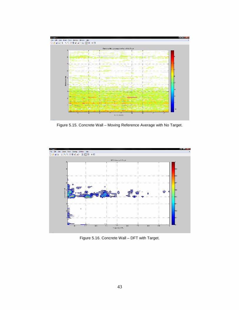
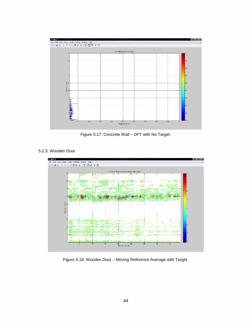
Figure 5.17 shows the plot using DFT method for Human target and No Target respectively.
Section 5.2.3 contains results for wooden door. Figure 5.18 and Figure 5.19 shows the plot
using Moving Average reference technique for cases with Human target and No target
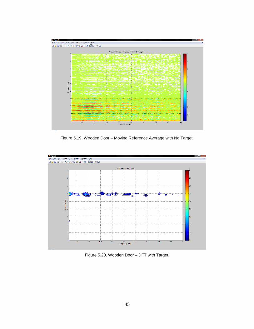
respectively. In Figure 5.18, the presence of human target at a distance of approximately 5.5 –
6 feet can be clearly seen. Figure 5.20 and Figure 5.21 shows the plot using DFT method for
Human target and No Target respectively.
5.2.1. Gypsum Wall
Figure 5.10. Gypsum Wall – Moving Reference Average with Target.
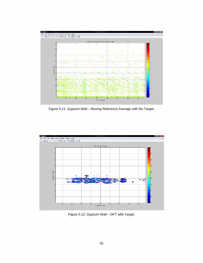
41
Figure 5.11. Gypsum Wall – Moving Reference Average with No Target.
Figure 5.12. Gypsum Wall – DFT with Target.
42
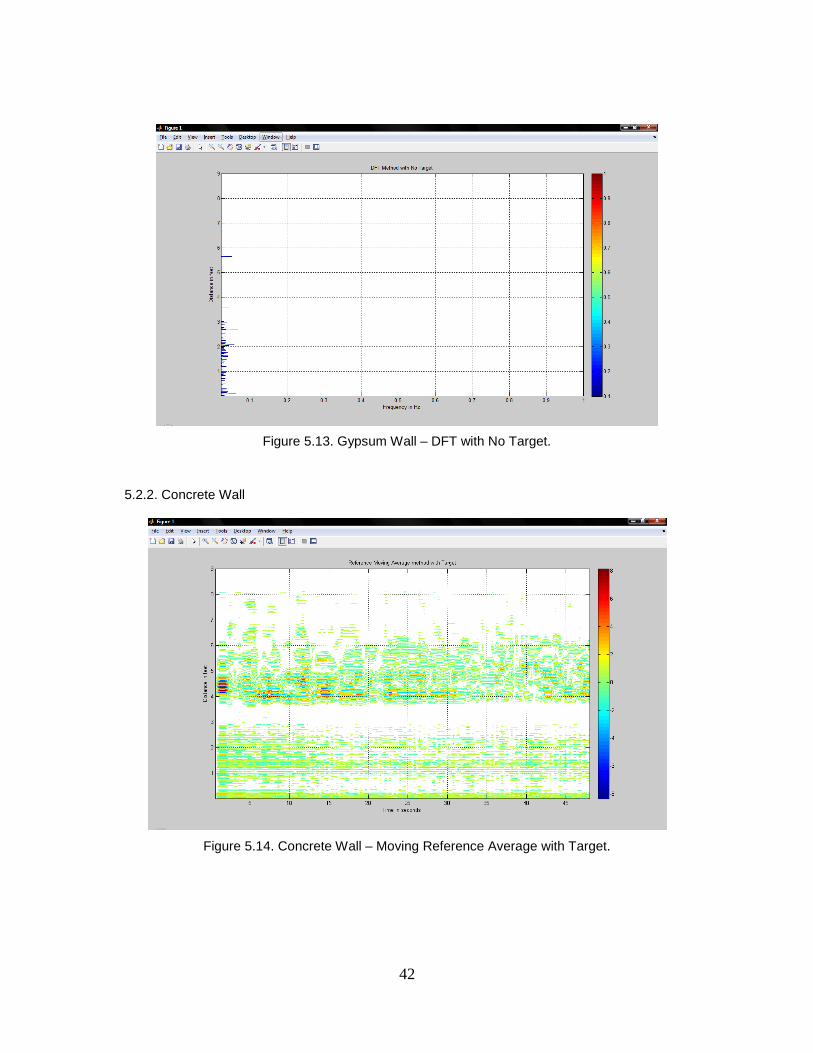
Figure 5.13. Gypsum Wall – DFT with No Target.
5.2.2. Concrete Wall
Figure 5.14. Concrete Wall – Moving Reference Average with Target.
43
Figure 5.15. Concrete Wall – Moving Reference Average with No Target.
Figure 5.16. Concrete Wall – DFT with Target.
44
Figure 5.17. Concrete Wall – DFT with No Target.
5.2.3. Wooden Door
Figure 5.18. Wooden Door – Moving Reference Average with Target.
45
Figure 5.19. Wooden Door – Moving Reference Average with No Target.
Figure 5.20. Wooden Door – DFT with Target.
46
Figure 5.21. Wooden Door – DFT with No Target.
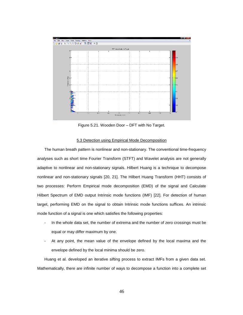
5.3 Detection using Empirical Mode Decomposition
The human breath pattern is nonlinear and non-stationary. The conventional time-frequency
analyses such as short time Fourier Transform (STFT) and Wavelet analysis are not generally
adaptive to nonlinear and non-stationary signals. Hilbert Huang is a technique to decompose
nonlinear and non-stationary signals [20, 21]. The Hilbert Huang Transform (HHT) consists of
two processes: Perform Empirical mode decomposition (EMD) of the signal and Calculate
Hilbert Spectrum of EMD output Intrinsic mode functions (IMF) [22]. For detection of human
target, performing EMD on the signal to obtain Intrinsic mode functions suffices. An intrinsic
mode function of a signal is one which satisfies the following properties:
- In the whole data set, the number of extrema and the number of zero crossings must be
equal or may differ maximum by one.
- At any point, the mean value of the envelope defined by the local maxima and the
envelope defined by the local minima should be zero.
Huang et al. developed an iterative sifting process to extract IMFs from a given data set.
Mathematically, there are infinite number of ways to decompose a function into a complete set

47
of components. The ones that give us more physical insight are more significant. In general, the
fewer the number of representing components, the higher is the information content. EMD is an
adaptive method that can generate many set of IMF components to represent the original data.
The EMD identifies intrinsic oscillatory modes by their characteristic time scales in the data
empirically. It separates the intrinsic mode functions (IMFs) from the original signal one by one,
until the residue is monotonic. The original signal is thus decomposed into a finite and a small
number of IMFs [20]. The flowchart of the decomposition process is described in [22]. The IMFs
which contain the micro-Doppler information can be extracted and the IMFs which contain
clutter and noise are discarded. This greatly improves the signal-to-clutter-ratio (SCR). The
extracted IMFs all admit well-behaved Hilbert transforms. Each IMF can thus be represented by
its analytic signal as shown in Figure 5.22 [23].
Figure 5.22. Representation of IMF by analytic signal.
48
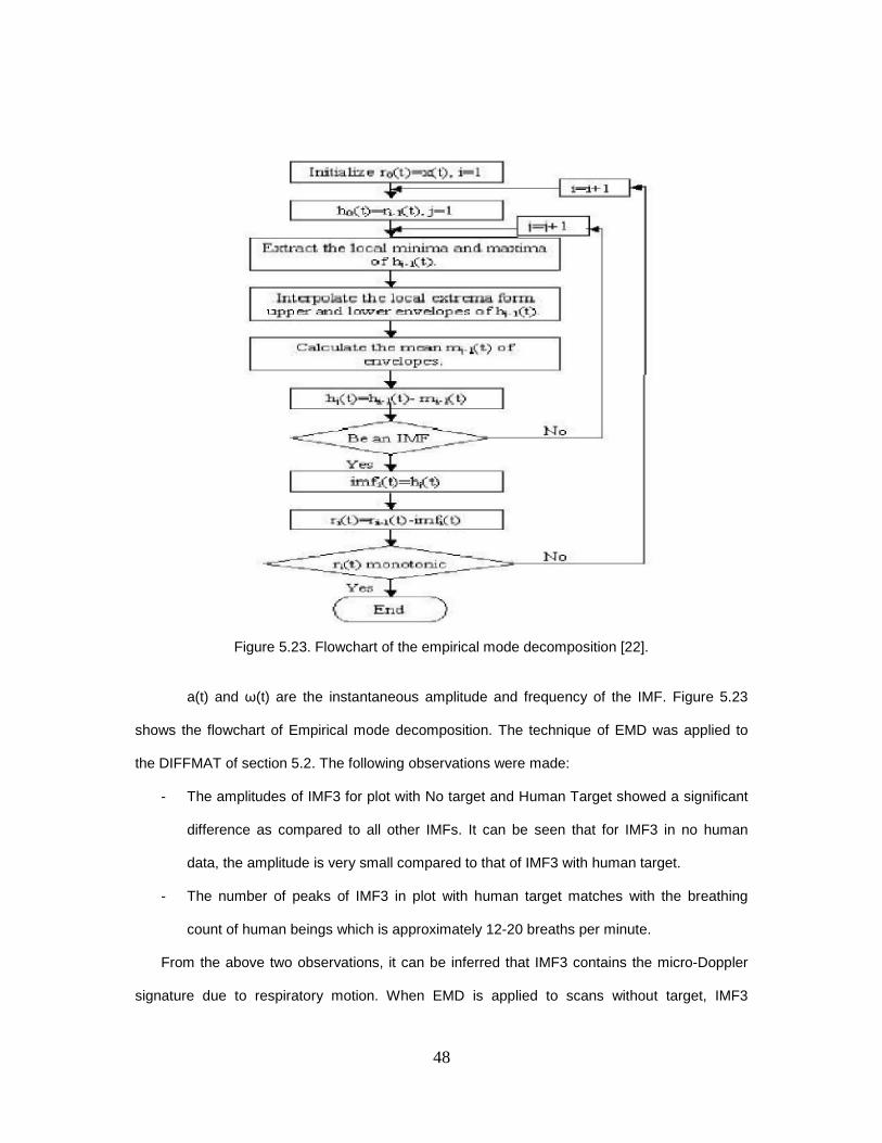
Figure 5.23. Flowchart of the empirical mode decomposition [22].
a(t) and ω(t) are the instantaneous amplitude and frequency of the IMF. Figure 5.23
shows the flowchart of Empirical mode decomposition. The technique of EMD was applied to
the DIFFMAT of section 5.2. The following observations were made:
- The amplitudes of IMF3 for plot with No target and Human Target showed a significant
difference as compared to all other IMFs. It can be seen that for IMF3 in no human
data, the amplitude is very small compared to that of IMF3 with human target.
- The number of peaks of IMF3 in plot with human target matches with the breathing
count of human beings which is approximately 12-20 breaths per minute.
From the above two observations, it can be inferred that IMF3 contains the micro-Doppler
signature due to respiratory motion. When EMD is applied to scans without target, IMF3

49
contains clutter. Hence, by employing Empirical mode decomposition from Hilbert-Huang
transform, the existence of human target can clearly be detected. But the range information
associated with it cannot be deduced and it is ambiguous.
Section 5.3.1 contains results for Gypsum wall. Fig 5.24 and 5.25 gives the IMF1-4
information for No target and human target respectively. The breathing Doppler signature is
present in IMF3 and peaks can be observed in Fig 5.27. Section 5.3.2 contains results for
Concrete wall. Fig 5.28 and 5.29 gives the IMF1-4 information for No target and human target
respectively. The breathing Doppler signature is present in IMF3 and peaks can be observed in
Fig 5.31. Section 5.3.3 contains results for wooden door. Fig 5.32 and 5.33 gives the IMF1-4
information for No target and human target respectively. The breathing Doppler signature is
present in IMF3 and peaks can be observed in Fig 5.35.
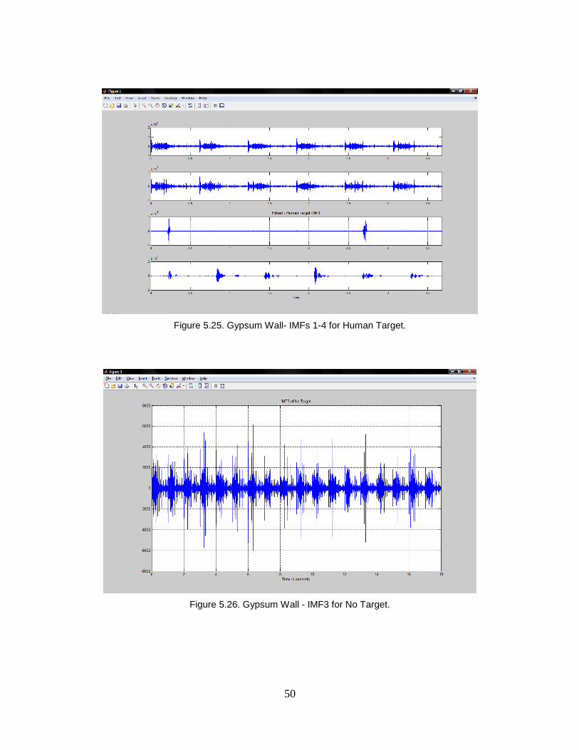
5.3.1. Gypsum Wall
The number of peaks in Fig 5.27 is 4 in 18 seconds which is about 13 per minute. This
matches with the average human breath rate which is 12-20 breath per minute.
Figure 5.24. Gypsum Wall - IMFs 1-4 for No Target.
50
Figure 5.25. Gypsum Wall- IMFs 1-4 for Human Target.
Figure 5.26. Gypsum Wall - IMF3 for No Target.

51
Figure 5.27. Gypsum Wall - IMF3 for Human Target (Peaks = 4 in 18 seconds).
5.3.2. Concrete Wall
The number of peaks in Fig 5.31 is 5 in 18 seconds which is about 17 per minute. This
matches with the average human breath rate which is 12-20 breath per minute.
Figure 5.28. Concrete Wall - IMFs 1-4 for No Target.

52
Figure 5.29. Concrete Wall - IMFs 1-4 for Human Target.
Figure 5.30. Concrete Wall – IMF3 for No Target.

53
Figure 5.31. Concrete Wall - IMF3 for Human Target (Peaks = 5 in 18 seconds).
5.3.3. Wooden Door
The number of peaks in Fig 5.35 is 8 in 36 seconds which is about 13 per minute. This
matches with the average human breath rate which is 12-20 breath per minute.
Figure 5.32. Wooden Door – IMFs 1-4 for No Target.

54
Figure 5.33. Wooden Door – IMFs 1-4 for Human Target.
Figure 5.34. Wooden Door – IMF3 for No Target.

55
Figure 5.35. Wooden Door – IMF3 for Human Target (Peaks = 8 in 36 seconds).
56
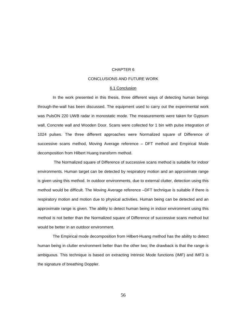
CHAPTER 6
CONCLUSIONS AND FUTURE WORK
6.1 Conclusion
In the work presented in this thesis, three different ways of detecting human beings
through-the-wall has been discussed. The equipment used to carry out the experimental work
was PulsON 220 UWB radar in monostatic mode. The measurements were taken for Gypsum
wall, Concrete wall and Wooden Door. Scans were collected for 1 bin with pulse integration of
1024 pulses. The three different approaches were Normalized square of Difference of
successive scans method, Moving Average reference – DFT method and Empirical Mode
decomposition from Hilbert Huang transform method.
The Normalized square of Difference of successive scans method is suitable for indoor
environments. Human target can be detected by respiratory motion and an approximate range
is given using this method. In outdoor environments, due to external clutter, detection using this
method would be difficult. The Moving Average reference –DFT technique is suitable if there is
respiratory motion and motion due to physical activities. Human being can be detected and an
approximate range is given. The ability to detect human being in indoor environment using this
method is not better than the Normalized square of Difference of successive scans method but
would be better in an outdoor environment.
The Empirical mode decomposition from Hilbert-Huang method has the ability to detect
human being in clutter environment better than the other two; the drawback is that the range is
ambiguous. This technique is based on extracting Intrinsic Mode functions (IMF) and IMF3 is
the signature of breathing Doppler.

57
The human detection in case of Gypsum wall and wooden door is better than Concrete
wall. This is due to the fact that the dielectric constant of concrete is higher. The range obtained
by the techniques used is slightly higher than the actual range since the electromagnetic wave
has to pass through the wall materials, thereby reducing the speed of the EM wave.
6.2 Future Work
The analysis carried out in this thesis was performed in an indoor environment. It
remains to be seen what would be the effect in the case of outdoor environment. Also, the effect
in case of the human being sitting or standing with back facing the wall needs to be attempted.
For wall EM mitigation, techniques like Wall parameter estimation, Cross polarization and
inverse scattering could be carried out. For accurate positioning and imaging of the human
being through the wall, three synchronized UWB radars would be needed.
58
APPENDIX A
BROADSPEC™ ANTENNA RADIATION PATTERN
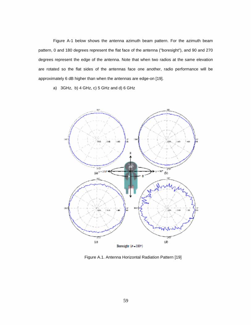
Figure A-1 below shows the antenna azimuth beam pattern
pattern, 0 and 180 degrees represent the flat face of the antenna ("boresight”), and 90 and 270
degrees represent the edge of the antenna. Note that when two radios at the sa
are rotated so the flat sides of the antennas face one another, radio performance will be
approximately 6 dB higher than when the antennas are edge
a) 3GHz, b) 4 GHz, c) 5 GHz and d) 6 GHz
Figure
59
1 below shows the antenna azimuth beam pattern. For the azimuth beam
pattern, 0 and 180 degrees represent the flat face of the antenna ("boresight”), and 90 and 270
degrees represent the edge of the antenna. Note that when two radios at the sa
are rotated so the flat sides of the antennas face one another, radio performance will be
n when the antennas are edge-on [19].
3GHz, b) 4 GHz, c) 5 GHz and d) 6 GHz
Figure A.1. Antenna Horizontal Radiation Pattern [19]
For the azimuth beam
pattern, 0 and 180 degrees represent the flat face of the antenna ("boresight”), and 90 and 270
degrees represent the edge of the antenna. Note that when two radios at the same elevation
are rotated so the flat sides of the antennas face one another, radio performance will be

60
Figure A-2 illustrates the elevation beam pattern [19]
a) 3GHz, b) 4 GHz, c) 5 GHz and d) 6 GHz
Figure A.2. Antenna Vertical Radiation Pattern [19]

61
REFERENCES
[1] Zaikov, Egor; , "UWB radar for detection and localization of trapped people," Radar
Symposium (IRS), 2010 11th International , vol., no., pp.1-4, 16-18 June 2010.
[2] Yarovoy, A.G.; Matuzas, J.; Levitas, B.; Ligthart, L.P.; , "UWB radar for human being
detection," Radar Conference, 2005. EURAD 2005. European , vol., no., pp.85-88, 6-7 Oct.
2005.
[3] Jeffrey H. Reed.An Introduction to Ultra Wideband Communication Systems, ISBN-10:
0131481037.
[4] Federal Communications Commission (FCC),"Revision of part 15 of the commission’s rules
regarding ultra-wideband transmission systems”, First Report and Order, ET Docket 98-153,
FCC 02-48; Adopted: February 2002; Released: April2002.
[5] R. A. Scholtz, “Multiple Access with Time-Hopping Impulse Modulation,” Proc. IEEE 1993
Milit. Comm. Conf., pp. 457-450.
[6] M.Hämäläinen, R.Tesi, J.Iinatti: "On the UWB System Performance Studies in AWGN
Channel with Interference in UMTS Band", IEEE Conference on Ultra Wideband Systems
and Technologies, UWBST2002, Baltimore, MD,USA, May 21-23, 2002, pp. 321-325,
http://ee.oulu.fi/~mattih/Hamalainen_UWBST02.pdf
[7] M.Hämäläinen, V.Hovinen, R.Tesi, J.Iinatti, M. Latva-aho: "On the UWB System
Coexistence with GSM900, UMTS/WCDMA, and GPS",IEEE Journal on Selected Areas in
Communications, Dec. 2002, Vol. 20, Number 9, pp- 1712-1721,
http://ee.oulu.fi/~mattih/JSAC_Dec2002.pdf
[8] H F Harmuth, Antennas and Waveguides for Nonsinusoidal Waves. New York: Academic,
1984.
62
[9] Robert A. Scholtz , David M. Pozar , Won Namgoong, Ultra-wideband radio, EURASIP
Journal on Applied Signal Processing, 2005, p.252-272, 1 January 2005.
[10] Time Domain Corporation , "PulsON® Technology Overview", July 2001.
[11] LAI, C. P., NARAYANAN, R. M., & CULKOWSKI, G. (2006). Through Wall Surveillance
Using Ultrawideband Random Noise Radar. Ft. Belvoir, Defense Technical Information
Center. http://handle.dtic.mil/100.2/ADA481425.
[12] Cengiz ALABACAK , "ANALYSIS OF ULTRA WIDE BAND (UWB) TECHNOLOGY FOR AN
INDOOR GEOLOCATION AND PHYSIOLOGICAL MONITORING SYSTEM", 2002.
[13] Leonard E. Miller, "Why UWB? A Review of Ultra wideband Technology," NETEX Project
Office,DARPA, April 2003.
[14] Ing. Michal Aftanas, “THROUGH WALL IMAGING WITH UWB RADAR SYSTEM”, August,
2009.
[15] Time Domain Corporation, "Apparatus, System and Method for FLIP modulation in an
Impulse radio Communication system", August 2005.
[16] R.M. Narayanan, "Through wall radar imaging using UWB noise waveforms," J. Franklin
Inst., vol.345, no. 6, July 2008.
[17] R Chandra, Abhay N Gaikwad, Dharmendra Singh and M J Nigam, "An approach to
remove the clutter and detect the target for ultra-wideband through-wall imaging," Journal
of Geophysics and Engineering, December 2008.
[18] Time Domain Corporation, "Monostatic Radar (MSR) Analysis Tool Application Note", May
2008.
[19] Time Domain Corporation, "PulsON 220 SAM User’s Manual", May 2008.
[20] Lai, Chieh-Ping; Ruan, Qing; Narayanan, Ram M.;"Hilbert-Huang Transform (HHT)
Processing of Through-Wall Noise Radar Data for Human Activity Characterization," Signal
Processing Applications for Public Security and Forensics, 2007. SAFE '07. IEEE
63
Workshop on , vol., no., pp.1-6, 11-13 April 2007.
[21] Ram M. Narayanan, Through-wall radar imaging using UWB noise waveforms, Journal of
the Franklin Institute, Volume 345, Issue 6, Advances in Indoor Radar Imaging, September
2008, Pages 659-678, ISSN 0016-0032, DOI: 10.1016/j.jfranklin.2008.03.004.
[22] N.E. Huang, Z. Shen, S.R. Long, M.C. Wu, H.H. Shih, Q. Zheng, N.C.Yen, C.C. Tung, and
H.H. Liu, "The empirical mode decomposition and the Hilbert spectrum for nonlinear and
non-stationary time series analysis," Proceedings of the Royal Society Of London Series A
- Mathematical Physical and Engineering Sciences, vol. 454, pp. 903-995, March 1998.
[23] Lai, Chieh-Ping; Ruan, Qing; Narayanan, Ram M.; , "Hilbert-Huang Transform (HHT)
Processing of Through-Wall Noise Radar Data for Human Activity Characterization," Signal
Processing Applications for Public Security and Forensics, 2007. SAFE '07. IEEE
Workshop on Vol.,no., pp.1-6, 11-13 April 2007.
64
BIOGRAPHICAL INFORMATION
Ashith Kumar was born in Udupi, India in 1984. He completed his Bachelor’s in
Telecommunication Engineering from the Visvesvaraya Technological University, India in 2006.
He worked at Infosys Technologies Ltd, India as a Software Engineer for two years prior to
joining the University of Texas at Arlington, Texas to pursue his Masters in Electrical
Engineering. Ashith worked as an intern at The Mathworks Inc, for seven months working with
the Embedded Links and Targets group. His research interests lies in various aspects of
Wireless Communications, Information Theory and Coding and Embedded systems. He is a
member of IEEE.
![Vortex Actuation via Electric Ducted Fans: an Experimental ...1246333/FULLTEXT01.pdf · most recent being the Wall-Climbing Robots (WCRs) [5]. Although the WCRs presented in the related](https://cdn.vdocuments.net/doc/165x107/5eda7a87b3745412b5716966/vortex-actuation-via-electric-ducted-fans-an-experimental-1246333fulltext01pdf.jpg)


