
EXPLORING THE BEHAVIOR OF
ATMOSPHERIC MOTION VECTOR (AMV)
ERRORS THROUGH SIMULATION STUDIES
Steve Wanzong and Chris Velden
University of Wisconsin - Madison
Cooperative Institute for Meteorological Satellite Studies
With contributions from Allen Huang, Mat Gunshor, Jason Otkin, Tom Greenwald
Jamie Daniels (NOAA/NESDIS)
Wayne Bresky (IM Systems Group, Inc.)
Tenth International Winds WorkshopTokyo, Japan
22 - 26 February 2010

Study Content
• Motivation
• Simulated GOES-R ABI Data Methodology
• Simulated ABI AMVs
• Analysis Strategy (Imposed Noise Effects)
• Comparison to WRF Model Wind Fields
• Summary

Study MotivationGOES-R Advanced Baseline Imager (ABI) -- Expected Launch in ~2017
What effect would imposed noise at spec, and over-spec, have on the
derived AMV product?ABI Current GOES Imager
Spectral coverage
16 bands 5 bands
Spatial resolution 0.64 µm Visible 0.5 km Approx. 1 km
Other Visible/near-IR 1.0 km n/a
Bands (>2 µm) 2 km Approx. 4 km
Spatial coverageFull disk 4 per hour Scheduled (3 hrly)
CONUS 12 per hour ~4 per hour
Mesoscale Every 30 sec n/a
Visible (reflective bands)
On-orbit calibration Yes No

ABI Simulations - Methodology
• Employ the high resolution Weather Research
and Forecasting (WRF) mesoscale model to generate simulated atmospheres.
• Calculate Top of Atmosphere (TOA) infrared
radiances from the WRF model simulations using CRTM and SOI for ABI bands 7-16 (LW Infrared).
• Calculate TOA reflectances from the WRF model
simulations using CRTM and SOI for ABI bands 1-6 (Visible/near-Infrared bands).
• Use automated feature-tracking software to derive AMVs from the simulated fields.

5
ABI bands via WRF simulation

GOES-R ABI – CONUS Coverage
Band 14: 11.2 μμμμm
Simulated GOES-R ABI
Simulated GOES-R ABI
Band 08: 6.19 μμμμm
GOES-12 Imager
GOES-12 Imager
Band 04: 10.7 μμμμm
Band 03: 6.5 μμμμm

Simulated AMVs:Simulated AMVs:Retrieval and Analysis StrategyRetrieval and Analysis Strategy
1.1. Obtain a set of 3 precisely calibrated, navigated and coObtain a set of 3 precisely calibrated, navigated and co--registered simulated images from the WRF model output for registered simulated images from the WRF model output for selected spectral channels (selected spectral channels (““purepure”” dataset = baseline dataset = baseline ““truthtruth””))
2.2. Employ the CIMSS/NESDIS automated AMV derivation Employ the CIMSS/NESDIS automated AMV derivation algorithm to target, height assign, track, and QC AMV fields algorithm to target, height assign, track, and QC AMV fields from these simulated imagesfrom these simulated images
3.3. Redo 1) above, except with introduced noise effects that Redo 1) above, except with introduced noise effects that represent proposed GOESrepresent proposed GOES--R satellite specs, and 3X specs. R satellite specs, and 3X specs. The noise includes striping, calibration and navigation offsetsThe noise includes striping, calibration and navigation offsets
4.4. Redo 2) above for each imposed noise AMV sampleRedo 2) above for each imposed noise AMV sample
5.5. Perform a quantitative error analysis on the resultant AMV Perform a quantitative error analysis on the resultant AMV fields using an objective toolkit called GRAFIIR, to deduce the fields using an objective toolkit called GRAFIIR, to deduce the effects of the imposed instrument noise on the derived AMV effects of the imposed instrument noise on the derived AMV products.products.

Imposed ABI Navigation Error -
Methodology
• The GOES-R PORD specification for navigation error is +/- 21 microradians (0.75 km).
• Each pixel is given a random compass direction and
a random normally distributed (about 0) shift the equivalent of 21 microradians.
• New pixel positions are generated using the random shift and random direction.
• The radiances are then linearly interpolated to these new positions from the original pixel locations.
• Second experiment: 3X Spec

GOES-R ABI – NavError (3Xspec)
Band 14 (11.2 μm)
Baseline
NavError3x

GOES-R ABI – NavError (3Xspec)IR-W AMVs - 5 minute time step
Yellow AMVs – “truth”
Blue AMVs -- NavError3x
Low-level High-level
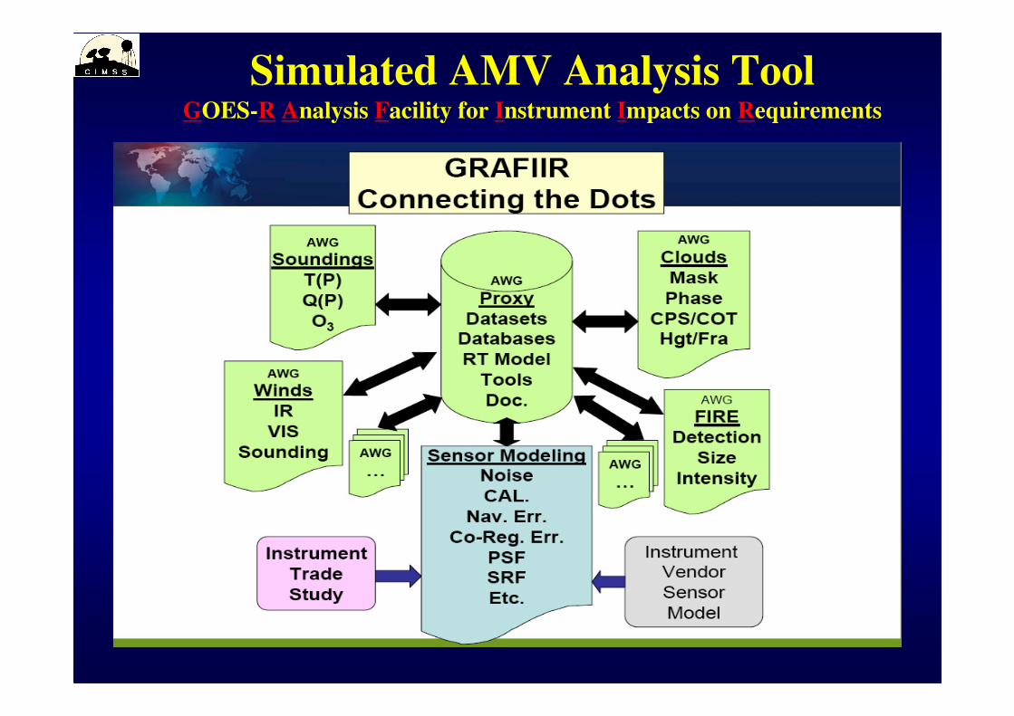
Simulated AMV Analysis ToolGOES-R Analysis Facility for Instrument Impacts on Requirements

GOES-R ABI Simulated AMV
Comparison MetricsAll AMVs are QI>80, and compared against WRF model winds
MVD =1
N(VD
i
i= 1
N
∑ )
SD =1
N(( VD
i
i= 1
N
∑ ) − ( MVD )) 2
Where:
(VD )i
= (Ui− U
r) 2
+ (Vi− V
r)2
Ui and Vi -> AMVUr and Vr -> “Truth”

GOESGOES--R ABI R ABI -- Comparison Statistics Comparison Statistics AMVs Derived from ABI Simulated Imagery AMVs Derived from ABI Simulated Imagery
vs. WRF Model Windsvs. WRF Model Winds
05 min – IR (11.2 μμμμm) 15 min – IR (11.2 μμμμm)
MVD
Count
7.5 m/s

GOESGOES--R ABI R ABI -- Comparison Statistics Comparison Statistics AMVs derived from ABI Simulated Imagery AMVs derived from ABI Simulated Imagery
vs. WRF Model Windsvs. WRF Model Winds
05 min – IR (11.2 μμμμm) 15 min – IR (11.2 μμμμm)
Std Dev
Count
3.8 m/s

Imposed ABI Striping Error -
Methodology
• The GOES-R PORD spec for striping error is that it should be less than the spec instrument noise.
• Assume a detector array (100 high) has 1 line simulated to be “bad”.
• Every 100th line has striping error applied by adding a radiance offset equal to the spec noise.
• Second experiment with 3X spec.

Temperature difference between “truth” and 3x Striping
Green is zero difference. Blue stripes are only observed difference.
Band 08 - 6.19 μm
GOES-R ABI – Striping3x

GOES-R ABI – Striping3x15 minute time step Clear sky water vapor tracking
Baseline (no striping) AMVsBand 08 (6.19 μm)
Striping3x Band 08 AMVs

GOES-R ABI – Striping3x15 minute time step Clear sky water vapor tracking
Baseline (no striping) AMVs Band 08 (6.19 μm) White areas -- tracking striping
Striping3x Band 08 AMVs

GOESGOES--R ABI R ABI -- Comparison Statistics Comparison Statistics AMVs derived from ABI Simulated Imagery AMVs derived from ABI Simulated Imagery
vs. WRF Model Windsvs. WRF Model Winds
15 min – WV (6.19 μμμμm)
MVD
Count
7.5 m/s
30 min – WV (6.19 μμμμm)

GOESGOES--R ABI R ABI -- Comparison Statistics Comparison Statistics AMVs derived from ABI Simulated Imagery AMVs derived from ABI Simulated Imagery
vs. WRF Model Windsvs. WRF Model Winds
Std Dev
Count
3.8 m/s
15 min – WV (6.19 μμμμm) 30 min – WV (6.19 μμμμm)

21
0.64 µµµµm 0.86 µµµµm 1.38 µµµµm
1.61 µµµµm 2.26 µµµµm 3.9 µµµµm 6.19 µµµµm
6.95 µµµµm 7.34 µµµµm
0.47 µµµµm
8.5 µµµµm 9.61 µµµµm
10.35 µµµµm 11.2 µµµµm 12.3 µµµµm 13.3 µµµµm
GO
ES
-R A
BI
Sim
ula
tio
ns o
f H
urr
ican
e K
atr
ina

-- Hurricane Katrina -- Atmospheric Motion Vectors from WRF Modelusing GOES-R ABI Simulated Radiances
Mid-Upper Levels
Low Levels

-- Hurricane Katrina -- Atmospheric Motion Vectors from WRF Modelusing GOES-R ABI Simulated Radiances
Mid-Upper LevelsGFS Background

24
Simulated Katrina
15-Minute Time Step15x15 Target Box Size
2 km Resolution
Mid-Upper LevelsLow Levels
5-Minute Time Step
15x15 Target Box Size2 km Resolution
Mid-Upper LevelsLow Levels

25
Simulated Katrina
15-Minute Time Step15x15 Target Box Size
4 km Resolution
Mid-Upper LevelsLow Levels
15-Minute Time Step
15x15 Target Box Size2 km Resolution
Mid-Upper LevelsLow Levels

Summary
• Simulated ABI data produced from WRF model TOA radiances is an effective way to study the potential effects of various ‘noise’ sources and processing choices on AMVs.
• Unaltered radiance fields were used as the baseline (“truth”) AMV product.
• Imposed navigation/registration errors have the greatest negative impact on IR and Visible AMVs compared to baseline.
• Striping effects are troublesome for clear sky water vapor AMVs.
• The above findings are effectively quantified using the GRAFIIR data analysis tool.

Thank You
Questions?

Backups


