Face Recognition

Ying Wuyingwu@ece.northwestern.edu

Electrical and Computer EngineeringNorthwestern University, Evanston, IL

http://www.ece.northwestern.edu/~yingwu

Recognizing Faces?

Lighting

View

Outline

Bayesian Classification Principal Component Analysis (PCA) Fisher Linear Discriminant Analysis (LDA) Independent Component Analysis (ICA)

Bayesian Classification

Classifier & Discriminant Function Discriminant Function for Gaussian Bayesian Learning and Estimation

Classifier & Discriminant Function

Discriminant function gi(x) i=1,…,C Classifier

Example

Decision boundary

ij )()( if xgxgx jii

)(ln)|(ln)(

)(|)|()(

)|()(

iii

iii

ii

pxpxg

pxpxg

xpxg

The choice of D-function is not unique

Multivariate Gaussian

),(~)( Nxp

principal axes

The principal axes (the direction) are given by the eigenvectors of ;

The length of the axes (the uncertainty) is given by the eigenvalues of

x1

x2

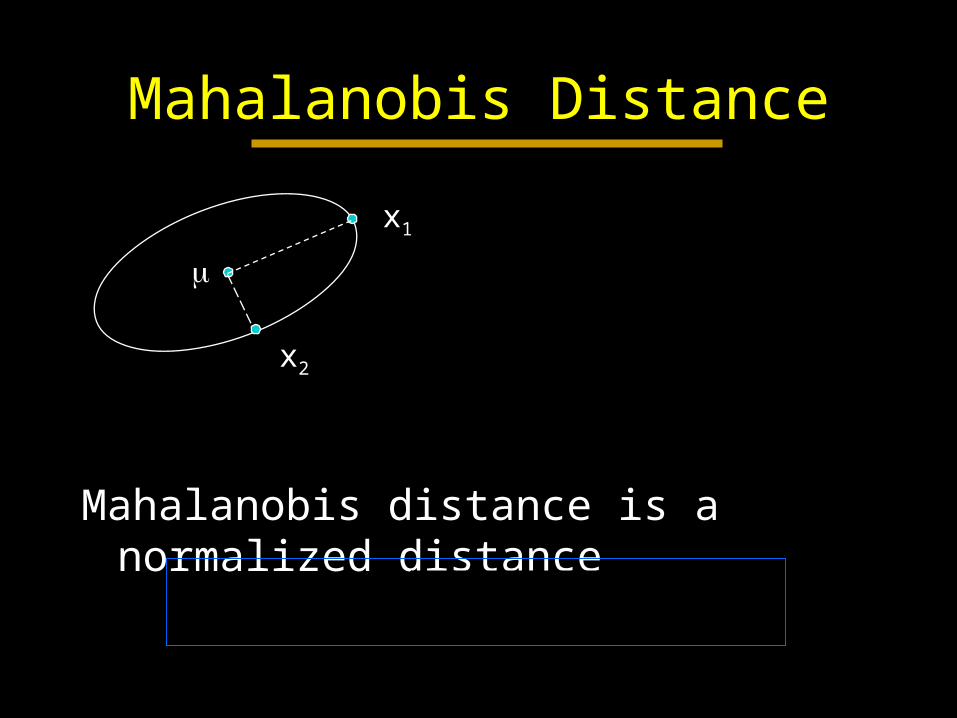
Mahalanobis Distance

Mahalanobis distance is a normalized distance

x1

x2

2221 |||||||| xx

MM xx |||||||| 21

)()(|||| 1 xxcx TM

Whitening Whitening:

– Find a linear transformation (rotation and scaling) such that the covariance becomes an identity matrix (i.e., the uncertainty for each component is the same)

y1

y2

x1

x2

y=ATx

p(x) ~ N(, ) p(y) ~ N(AT, ATA)

UUUA TT

e wher :solution 2

1

Disc. Func. for Gaussian

Minimum-error-rate classifier

)(ln||ln2

12ln

2)()(

2

1)(

)(ln)|(ln)(

1iiii

Tii

iii

pd

xxxg

pxpxg

Case I: i = 2I

)(ln22

1)(ln

2

||||)(

22

2

iTi

Ti

Ti

ii pxxxp

xxg

0

22)(ln

2

11)(

iT

i

iTi

T

ii

WxW

pxxg

constant

Liner discriminant function

Boundary:

)(ln)(

where0)( )(

)()(

||||21

0

0

2

2

jipp

ji

ji

Tji

j

i

jix

W

xxWgxg

Example

Assume p(i)=p(j)

i

j

Let’s derive the decision boundary:

02

)(

jiT

ji x

Case II: i= )(ln)()()( 1

21

iiT

ii pxxxg

0

1211 ))(ln()()(

iT

i

iiTi

Tii

WxW

pxxg

)())(

)(ln)(ln)(

2

1

)(

where0)(

10

1

0

jiji

Tji

jiji

ji

T

ppx

W

xxW

The decision boundary is still linear:

Case III: i= arbitrary

)(ln||ln

where)(

211

21

0

1

121

0

iiiiTii

iii

ii

iT

iiT

i

pW

W

A

WxWxAxxg

The decision boundary is no longer linear, but hyperquadrics!

Bayesian Learning

Learning means “training” i.e., estimating some unknowns from

“training data” WHY?

– It is very difficult to specify these unknowns– Hopefully, these unknowns can be recovered

from examples collected.

Maximum Likelihood Estimation

Collected examples D={x1,x2,…,xn}

Estimate unknown parameters in the sense that the data likelihood is maximized

Likelihood Log Likelihood

ML estimation

n

kkxpDp

1

)|()|(

)|(maxarg)|(maxarg*

DLDp

n

kkxpDpL

1

)|(ln)|(ln)(

Case I: unknown

)()(|]|)2ln[()|(ln 121

21

kT

kd

k xxxp

n

kk

n

kk

kk

xn

x

xxp

11

1

1

1ˆ 0)ˆ(

)()|((ln

Case II: unknown and 22

21

21 let )(2ln),|(ln kk xxp

2

2

2

)(

2

1),|(ln

)(1),|(ln

kk

kk

xxp

xxp

0ˆ

)ˆ(ˆ1

0)ˆ(ˆ1

12

2

1

1

n

k

kn

k

k

n

k

x

x

n

kk

n

kk

xn

xn

1

222

1

)ˆ(1ˆˆ

1ˆ

Tk

n

kk

n

kk

xxn

xn

)ˆ()ˆ(1ˆ

1ˆ

1

1

generalize

Bayesian Estimation

Collected examples D={x1,x2,…,xn}, drawn independently from a fixed but unknown distribution p(x)

Bayesian learning is to use D to determine p(x|D), i.e., to learn a p.d.f.

p(x) is unknown, but has a parametric form with parameters ~ p()

Difference from ML: in Bayesian learning, is not a value, but a random variable and we need to recover the distribution of , rather than a single value.

Bayesian Estimation

This is obvious from the total probability rule, i.e., p(x|D) is a weighted average over all

If p( |D) peaks very sharply about some value *, then p(x|D) ~ p(x| *)

dDpxpdDxpDxp )|()|()|,()|(

The Univariate Case

assume is the only unknown, p(x|)~N(, 2) is a r.v., assuming a prior p() ~ N(0, 0

2), i.e., 0 is the best guess of , and 0 is the uncertainty of it.

),(~)( ),,(~)|( where

)()|()()|()|(

20

2

1

ok

n

kk

NpNxp

pxppDpDp

kk

n xDp

)(2(exp)|( 2

0222

12121

P(|D) is also a Gaussian for any # of training examples

The Univariate Case

220

2202

0220

2

220

20

n

2

ˆ

have we

),(~)|(let weif

n

nn

n

NDp

n

n

nn

The best guess for after observing n examples

n measures the uncertainty of this guess after observing n examples

n=1

n=5

n=10

n=30

p(|x1,…,xn) p(|D) becomes more and more sharply peaked when observing more and more examples, i.e., the uncertainty decreases.

nn

22

The Multivariate Case

),(~)( ),(~)|( 00 NpNxp

n

kkn

nnn

nnnnn

nn

xn

NDp

1

11100

011

0111

00

1ˆ where

)(

ˆ)(ˆ)(

have we),,(~)|(let

),(~)|()|()|( and nnNdDpxpDxp

PCA and Eigenface

Principal Component Analysis (PCA) Eigenface for Face Recognition

PCA: motivation

Pattern vectors are generally confined within some low-dimensional subspaces

Recall the basic idea of the Fourier transform– A signal is (de)composed of a linear combination

of a set of basis signal with different frequencies.

PCA: idea

emx

222

1

21

||||)(2||||

||)(||),,...,(

mxmxee

xemeJ

kkT

kk

n

kkkn

)( 0)(22 mxemxeJ

kT

kkT

kk

m

e x

xk

PCA

2

2

222

||||

||||))((

||||2)(

mxeSe

mxemxmxe

mxeJ

k

kT

kkT

kkk

1|||| s.t. maxarg)(minarg eSeeeJ T

ee

)1(maxarg* eeSeee TT

e

1 i.e., ,0 SeeeSe TTo maximize eTSe, we need to select max

Algorithm

Learning the principal components from {x1, x2, …, xn}

] ..., , [ (5)

u and sorting )4(

ion decomposit eigenvalue )3(

))(( (2)

] ..., ,[ ,1

)1(

21

i

1

11

Tm

TTT

i

T

Tn

k

Tkk

n

n

kk

uu,u P

UUS

AAmxmxS

mxmxAxn

m

PCA for Face Recognition

Training data D={x1, …, xM}– Dimension (stacking the pixels together to make a vector

of dimension N)

– Preprocessing cropping normalization

These faces should lie in a “face” subspace Questions:

– What is the dimension of this subspace?

– How to identify this subspace?

– How to use it for recognition?

Eigenface

The EigenFace approach: M. Turk and A. Pentland, 1992

An Issue

In general, N >> M However, S, the covariance matrix, is NxN! Difficulties:

– S is ill-conditioned. Rank(S)<<N– The computation of the eigenvalue decomposition

of S is expensive when N is large Solution?

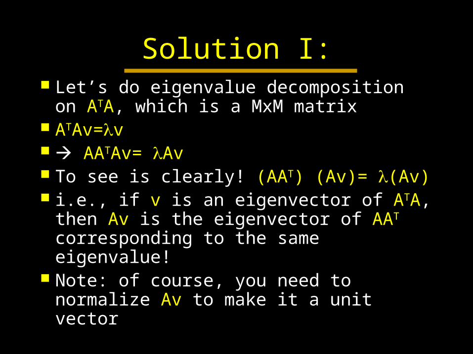
Solution I: Let’s do eigenvalue decomposition on ATA,

which is a MxM matrix ATAv=v AATAv= Av To see is clearly! (AAT) (Av)= (Av) i.e., if v is an eigenvector of ATA, then Av

is the eigenvector of AAT corresponding to the same eigenvalue!

Note: of course, you need to normalize Av to make it a unit vector

Solution II:

You can simply use SVD (singular value decomposition)

A = [x1-m, …, xM-m]

A = UVT

– A: NxM– U: NxM UTU=I : MxM diagonal – V: MxM VTV=VVT=I

Fisher Linear Discrimination

LDA PCA+LDA for Face Recognition

When does PCA fail?

PCA

Linear Discriminant Analysis

Finding an optimal linear mapping WFinding an optimal linear mapping W

Catches major difference between classes and Catches major difference between classes and discount irrelevant factorsdiscount irrelevant factors

In the mapped space, data are clusteredIn the mapped space, data are clustered

Within/between class scatters

2211

1

22

11

1

21

~ ,1~

:nsformlinear tra the

1 ,

1

mWmmWxWn

m

xWy

xn

mxn

m

T

Dx

TT

T

DxDx

TB

W

T

Yy

T

Yy

Dx

T

Dx

T

mmmmS

SSS

WSWmySWSWmyS

mxmxSmxmxS

))(( :scatter classbetween

:scatter classwithin

)~(~

,)~(~

))(( ,))((

2121

21

22

2212

11

222111

21

21

Fisher LDA

WSW

WSW

WSSW

WmmmmW

SS

mmWJ

WT

BT

T

TT

)(

))((~~

|~~|)(

21

2121

21

221

)(maxarg* WJWW

problem eigenvalue dgeneralize a is this )(max wSwSWJ WB

Solution I

If Sw is not singular

You can simply do eigenvalue decomposition on SW

-1SB

wwSS BW 1

Solution II

Noticing:– SBW is on the direction of m1-m2 (WHY?)

– We are only concern about the direction of the projection, rather than the scale

We have

)( 211 mmSw W

Multiple Discriminant Analysis

C

kkW

Dx

Tiii

Dxii

SS

mxmxS

xn

m

i

i

1

))((

,1

WSWmmmmnS

WSWS

mnn

m

mWyn

m

BT

C

k

TiiiB

WT

W

C

kkk

iT

Yyii

i

1

1

)~~)(~~(~

,~

,~1~

,1~

xWy T

||

||

|~

|

|~

|maxarg*

WSW

WSW

S

SW

WT

BT

W

B

W

iWiB wSwS

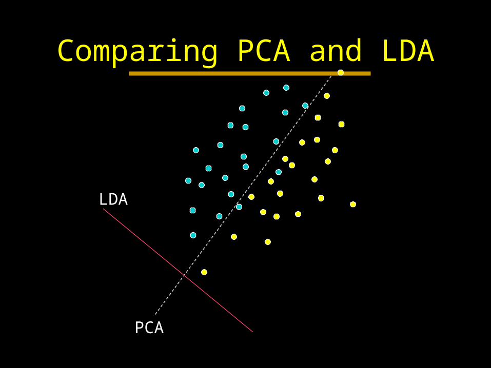
Comparing PCA and LDA

PCA

LDA

MDA for Face Recognition

Lighting

• PCA does not work well! (why?)

• solution: PCA+MDA

Independent Component Analysis

The cross-talk problem ICA

Cocktail party

t

S1(t)

S2(t)

t

t

x1(t)

t

x2(t)

t

x3(t)

A

Can you recover s1(t) and s2(t) from x1(t), x2(t) and x3(t)?

Formulation

ASXsaX

jsasaxn

iii

njnjj

or

...

1

11

Both A and S are unknowns!

Can you recover both A and S from X?

The Idea

y is a linear combination of {si} Recall the central limit theory! A sum of even two independent r.v. is more

Gaussian than the original r.v. So, ZTS should be more Gaussian than any of {si} In other words, ZTS become least Gaussian when

in fact equal to {si} Amazed!

SZASWXWY TTT

Face Recognition: Challenges

View