
Face Recognition
Jens Fagertun
Kongens Lyngby 2005Master Thesis IMM-Thesis-2005-74

Technical University of Denmark
Informatics and Mathematical Modelling
Building 321, DK-2800 Kongens Lyngby, Denmark
Phone +45 45253351, Fax +45 45882673
www.imm.dtu.dk

Abstract
This thesis presents a comprehensive overview of the problem of facial recogni-tion. A survey of available facial detection algorithms as well as implementationand tests of different feature extraction and dimensionality reduction methodsand light normalization methods are presented.
A new feature extraction and identity matching algorithm, the Multiple Indi-vidual Discriminative Models (MIDM) algorithm, is proposed.
MIDM is in collaboration with AAM-API, a C++ open source implementationof Active Appearance Models (AAM), implemented into the “FaceRec” Delphi7 application, a real time automatic facial recognition system. AAM is used forface detection and MIDM for face recognition.
Extensive testing of the MIDM algorithm is presented and its performance eval-uated by the Lausanne protocol. The Lausanne protocol is a precise and widelyaccepted protocol for the testing of facial recognition algorithms. These testevaluations showed that the MIDM algorithm is superior to all other algorithmsreported by the Lausanne protocol.
Finally, this thesis presents a description of 3D facial reconstruction from asingle 2D image. This is done by using prior knowledge in form of a statisticalshape model of faces in 3D.
Keywords: Face Recognition, Face Detection, Lausanne Protocol, 3D Face Re-construction, Principal Component Analysis, Fisher Linear Discriminant Anal-ysis, Locality Preserving Projections, Kernel Fisher Discriminant Analysis.

ii

Resume
Denne afhandling præsenterer et omfattende overblik over problemet ansigtsgenkendelse. En oversigt over de tilgængelige algoritmer til detektering af an-sigter savel som implementation og test af forskellige metoder til ekstraktion afegenskaber og dimensionsreduktion samt metoder til lysnormalisering præsen-teres.
En ny algoritme til ektraktion af egenskaber og matchning af identiteter (Mul-tiple Individual Discriminative Models - MIDM) er blevet foreslaet.
MIDM, sammen med AAM-API, en open-source C++ implementering af Ac-tive Appearance Models (AAM), er blevet implementeret som applikationen”FaceRec” i Delphi 7. Denne applikation er et automatisk system til ansigtsgenkendelse, der kører i sand tid. AAM er brugt til ansigts detektering ogMIDM er brugt til ansigts genkendelse.
Udførlig testning af MIDM algoritmen er præsenteret og dens ydelse evalueretved hjælp af Lausanne protokollen. Lausanne protokollen er en præcis og bredtaccepteret protokol for test af ansigts genkendelses algoritmer. Disse test eval-ueringer viste at MIDM algoritmen er alle andre algoritmer rapporteret vedhjælp af Lausanne protokollen overlegen.
Endeligt, præsenterer denne afhandling en beskrivelse af 3D ansigts rekonstruk-tion fra et enkelt 2D billede. Dette er gjort ved at bruge a priori kendskab iform af en statistisk model for formen af ansigter i 3D.
Nøgleord: Ansigts Genkendelse, Ansigts Detektering, Lausanne Protokollen,3D Ansigts Rekonstruktion, Principal Komponent Analyse, Fisher Linear Dis-

iv
kriminant Analyse, Locality Preserving Projections, Kernel Fisher DiskriminantAnalyse.

Preface
This thesis was prepared at the Section for Image Analysis, in the Departmentof Informatics and Mathematical Modelling, IMM, located at the TechnicalUniversity of Denmark, DTU, as a partial fulfillment of the requirements foracquiring the degree Master of Science in Engineering, M.Sc.Eng.
The thesis deals with different aspects of face recognition using both the geo-metrical and photometrical information of facial images. The main focus willbe on face recognition from 2D images, but 2D to 3D conversion of data willalso be considered.
The thesis consists of this report, a technical report and two papers; one pub-lished in Proceedings of the 14th Danish Conference on Pattern Recognition andImage Analysis and one submitted to IEEE Transactions on Pattern Analysisand Machine Intelligence, written during the period January to September 2005.
It is assumed that the reader has a basic knowledge in the areas of statisticsand image analysis.
Lyngby, September 2005
Jens Fagertun[email: [email protected]]

vi

Publication list for this thesis
[20] Jens Fagertun, David Delgado Gomez, Bjarne K. Ersbøll and RasmusLarsen. A face recognition algorithm based on multiple individual dis-criminative models. Proceedings of the 14th Danish Conference on PatternRecognition and Image Analysis, 2005.
[21] Jens Fagertun and Mikkel B. Stegmann. The IMM Frontal Face Database.Technical Report, Informatics and Mathematical Modelling, TechnicalUniversity of Denmark, 2005.
[27] David Delgado Gomez, Jens Fagertun and Bjarne K. Ersbøll. A facerecognition algorithm based on multiple individual discriminative models.IEEE Transactions on Pattern Analysis and Machine Intelligence. Toappear - Submitted in 2005 - ID TPAMI-0474-0905.

viii

Acknowledgements
I would like to thank the following people for there support and assistance inmy preparation of the work presented in this thesis:
First and foremost, I thank my supervisor Bjarne K. Ersbøll for his supportthroughout this thesis. It has been an exciting experience and great opportunityto work with face recognition, a very interesting area in image analysis andpattern recognition.
I thank my co-supervisor Mikkel B. Stegmann for his huge initial support andalways having time to spare.
I thank my good friend David Delgado Gomez for all the productive conver-sations on different issues of face recognition, and for an excellent partnershipduring the writing of the two papers included in this thesis.
I thank Rasmus Larsen for his great patience when answering questions of astatistical nature.
I thank my office-mates Mads Fogtmann Hansen, Rasmus Engholm and SteenLund Nielsen for productive conversations and spending time answering myquestions, which has been a great help.
I thank Mette Christensen and Bo Langgaard Lind for proof-reading the manus-cript of this thesis.
I thank Lars Kai Hansen since he encouraged me to write my thesis at the image

x
analysis section.
In general I thank the staff of the image analysis- and computer graphics sectionfor providing a pleasant and inspiring atmosphere as well as for their participa-tion in the construction of the IMM Frontal Face Database.
Finally, I thank David Delgado Gomez and the Computational Imaging Lab atthe Department of Technology at Pompeu Fabra University, Barcelona for theirpartnership in the participation in the ICBA20061 Face Verification Contest inHong Kong in January, 2006.
1International Conference on Biometrics 2006.

xi

xii Contents

Contents
Abstract i
Resume iii
Preface v
Publication list for this thesis vii
Acknowledgements ix
1 Introduction 1
1.1 Motivation and Objectives . . . . . . . . . . . . . . . . . . . . . . 3
1.2 Thesis Overview . . . . . . . . . . . . . . . . . . . . . . . . . . . 4
1.3 Mathematical Notation . . . . . . . . . . . . . . . . . . . . . . . 5
1.4 Nomenclature . . . . . . . . . . . . . . . . . . . . . . . . . . . . . 6
1.5 Abbreviations . . . . . . . . . . . . . . . . . . . . . . . . . . . . . 7

xiv CONTENTS
I Face Recognition in General 9
2 History of Face Recognition 11
3 Face Recognition Systems 13
3.1 Face Recognition Tasks . . . . . . . . . . . . . . . . . . . . . . . 13
3.1.1 Verification . . . . . . . . . . . . . . . . . . . . . . . . . . 14
3.1.2 Identification . . . . . . . . . . . . . . . . . . . . . . . . . 14
3.1.3 Watch List . . . . . . . . . . . . . . . . . . . . . . . . . . 14
3.2 Face Recognition Vendor Test 2002 . . . . . . . . . . . . . . . . . 16
3.3 Discussion . . . . . . . . . . . . . . . . . . . . . . . . . . . . . . . 20
4 The Process of Face Recognition 21
4.1 Face Detection . . . . . . . . . . . . . . . . . . . . . . . . . . . . 22
4.2 Preprocessing . . . . . . . . . . . . . . . . . . . . . . . . . . . . . 22
4.3 Feature Extraction . . . . . . . . . . . . . . . . . . . . . . . . . . 23
4.4 Feature Matching . . . . . . . . . . . . . . . . . . . . . . . . . . . 23
4.5 Thesis Perspective . . . . . . . . . . . . . . . . . . . . . . . . . . 23
5 Face Recognition Considerations 25
5.1 Variation in Facial Appearance . . . . . . . . . . . . . . . . . . . 25
5.2 Face Analysis in an Image Space . . . . . . . . . . . . . . . . . . 26
5.2.1 Exploration of Facial Submanifolds . . . . . . . . . . . . . 27
5.3 Dealing with Non-linear Manifolds . . . . . . . . . . . . . . . . . 28

CONTENTS xv
5.3.1 Technical Solutions . . . . . . . . . . . . . . . . . . . . . . 28
5.4 High Input Space and Small Sample Size . . . . . . . . . . . . . . 30
6 Available Data 33
6.1 Face Databases . . . . . . . . . . . . . . . . . . . . . . . . . . . . 34
6.1.1 AR . . . . . . . . . . . . . . . . . . . . . . . . . . . . . . . 34
6.1.2 BioID . . . . . . . . . . . . . . . . . . . . . . . . . . . . . 34
6.1.3 BANCA . . . . . . . . . . . . . . . . . . . . . . . . . . . . 35
6.1.4 IMM Face Database . . . . . . . . . . . . . . . . . . . . . 35
6.1.5 IMM Frontal Face Database . . . . . . . . . . . . . . . . . 35
6.1.6 PIE . . . . . . . . . . . . . . . . . . . . . . . . . . . . . . 36
6.1.7 XM2VTS . . . . . . . . . . . . . . . . . . . . . . . . . . . 36
6.2 Data Sets Used in this Work . . . . . . . . . . . . . . . . . . . . 36
6.2.1 Data Set I . . . . . . . . . . . . . . . . . . . . . . . . . . . 37
6.2.2 Data Set II . . . . . . . . . . . . . . . . . . . . . . . . . . 37
6.2.3 Data Set III . . . . . . . . . . . . . . . . . . . . . . . . . . 41
6.2.4 Data Set IV . . . . . . . . . . . . . . . . . . . . . . . . . . 41
II Assessment 45
7 Face Detection: A Survey 47
7.1 Representative Work of Face Detection . . . . . . . . . . . . . . . 49
7.2 Description of Selected Face Detection Methods . . . . . . . . . . 49

xvi CONTENTS
7.2.1 General Aspects of Face Detections Algorithms . . . . . . 50
7.2.2 Eigenfaces . . . . . . . . . . . . . . . . . . . . . . . . . . . 50
7.2.3 Fisherfaces . . . . . . . . . . . . . . . . . . . . . . . . . . 51
7.2.4 Neural Networks . . . . . . . . . . . . . . . . . . . . . . . 51
7.2.5 Active Appearance Models . . . . . . . . . . . . . . . . . 52
8 Preprocessing of a Face Image 59
8.1 Light Correction . . . . . . . . . . . . . . . . . . . . . . . . . . . 59
8.1.1 Histogram Equalization . . . . . . . . . . . . . . . . . . . 59
8.1.2 Removal of Specific Light Sources based on 2D Face Models 60
8.2 Discussion . . . . . . . . . . . . . . . . . . . . . . . . . . . . . . . 62
9 Face Feature Extraction: Dimensionality Reduction Methods 65
9.1 Principal Component Analysis . . . . . . . . . . . . . . . . . . . 66
9.1.1 PCA Algorithm . . . . . . . . . . . . . . . . . . . . . . . . 66
9.1.2 Computational Issues of PCA . . . . . . . . . . . . . . . . 68
9.2 Fisher Linear Discriminant Analysis . . . . . . . . . . . . . . . . 69
9.2.1 FLDA in Face Recognition Problems . . . . . . . . . . . . 70
9.3 Locality Preserving Projections . . . . . . . . . . . . . . . . . . . 70
9.3.1 LPP in Face Recognition Problems . . . . . . . . . . . . . 73
9.4 Kernel Fisher Discriminant Analysis . . . . . . . . . . . . . . . . 73
9.4.1 Problems of KFDA . . . . . . . . . . . . . . . . . . . . . . 77
10 Experimental Results I 79

CONTENTS xvii
10.1 Illustration of the Feature Spaces . . . . . . . . . . . . . . . . . . 80
10.2 Face Identification Tests . . . . . . . . . . . . . . . . . . . . . . . 85
10.2.1 50/50 Test . . . . . . . . . . . . . . . . . . . . . . . . . . 85
10.2.2 Ten-fold Cross-validation Test . . . . . . . . . . . . . . . . 86
10.3 Discussion . . . . . . . . . . . . . . . . . . . . . . . . . . . . . . . 87
III Development 89
11 Multiple Individual Discriminative Models 91
11.1 Algorithm Description . . . . . . . . . . . . . . . . . . . . . . . . 92
11.1.1 Creations of the Individual Models . . . . . . . . . . . . . 92
11.1.2 Classification . . . . . . . . . . . . . . . . . . . . . . . . . 96
11.2 Discussion . . . . . . . . . . . . . . . . . . . . . . . . . . . . . . . 96
12 Reconstruction of 3D Face from a 2D Image 99
12.1 Algorithm Description . . . . . . . . . . . . . . . . . . . . . . . . 99
12.2 Discussion . . . . . . . . . . . . . . . . . . . . . . . . . . . . . . . 103
13 Experimental Results II 105
13.1 Overview . . . . . . . . . . . . . . . . . . . . . . . . . . . . . . . 105
13.1.1 Initial Evaluation Tests . . . . . . . . . . . . . . . . . . . 105
13.1.2 Lausanne Performance Tests . . . . . . . . . . . . . . . . 106
13.2 Initial Evaluation Tests . . . . . . . . . . . . . . . . . . . . . . . 106
13.2.1 Identification Test . . . . . . . . . . . . . . . . . . . . . . 106

xviii CONTENTS
13.2.2 The Important Image Regions . . . . . . . . . . . . . . . 108
13.2.3 Verification Test . . . . . . . . . . . . . . . . . . . . . . . 110
13.2.4 Robustness Test . . . . . . . . . . . . . . . . . . . . . . . 112
13.3 Lausanne Performance Tests . . . . . . . . . . . . . . . . . . . . . 113
13.3.1 Participants in the Face Verification Contest, 2003 . . . . 115
13.3.2 Results . . . . . . . . . . . . . . . . . . . . . . . . . . . . 116
13.4 Discussion . . . . . . . . . . . . . . . . . . . . . . . . . . . . . . . 118
IV Implementation 121
14 Implementation 123
14.1 Overview . . . . . . . . . . . . . . . . . . . . . . . . . . . . . . . 123
14.2 FaceRec . . . . . . . . . . . . . . . . . . . . . . . . . . . . . . . . 124
14.2.1 FaceRec Requirements . . . . . . . . . . . . . . . . . . . . 125
14.2.2 AAM-API DLL . . . . . . . . . . . . . . . . . . . . . . . . 125
14.2.3 Make MIDM Model File . . . . . . . . . . . . . . . . . . . 126
14.3 Matlab Functions . . . . . . . . . . . . . . . . . . . . . . . . . . . 126
14.4 Pitfalls . . . . . . . . . . . . . . . . . . . . . . . . . . . . . . . . . 127
14.4.1 Passing Arrays . . . . . . . . . . . . . . . . . . . . . . . . 127
14.4.2 The Matlab Eig Function . . . . . . . . . . . . . . . . . . 127

CONTENTS xix
V Discussion 129
15 Future Work 131
15.1 Light Normalization . . . . . . . . . . . . . . . . . . . . . . . . . 131
15.2 Face Detection . . . . . . . . . . . . . . . . . . . . . . . . . . . . 132
15.3 3D Facial Reconstruction . . . . . . . . . . . . . . . . . . . . . . 132
16 Discussion 133
16.1 Summary of Main Contributions . . . . . . . . . . . . . . . . . . 133
16.1.1 IMM Frontal Face Database . . . . . . . . . . . . . . . . . 133
16.1.2 The MIDM Algorithm . . . . . . . . . . . . . . . . . . . . 134
16.1.3 A Delphi Implementation . . . . . . . . . . . . . . . . . . 134
16.1.4 Matlab Functions . . . . . . . . . . . . . . . . . . . . . . . 134
16.2 Conclusion . . . . . . . . . . . . . . . . . . . . . . . . . . . . . . 135
A The IMM Frontal Face Database 143
B A face recognition algorithm based on MIDM 153
C A face recognition algorithm based on MIDM 163
D FaceRec Quick User Guide 173
E AAM-API DLL 177
F CD-ROM Contents 181

xx CONTENTS

Chapter 1
Introduction
Face recognition is a task so common to humans, that the individual does noteven notice the extensive number of times it is performed every day. Althoughresearch in automated face recognition has been conducted since the 1960’s, ithas only recently caught the attention of the scientific community. Many faceanalysis and face modeling techniques have progressed significantly in the lastdecade [30]. However, the reliability of face recognition schemes still poses agreat challenge to the scientific community.
Falsification of identity cards or intrusion of physical and virtual areas by crack-ing alphanumerical passwords appear frequently in the media. These problemsof modern society have triggered a real necessity for reliable, user-friendly andwidely acceptable control mechanisms for the identification and verification ofthe individual.
Biometrics, which is based on authentication on the intrinsic aspects of a spe-cific human being, appears as a viable alternative to more traditional approaches(such as PIN codes or passwords). Among the oldest biometric techniques isfingerprint recognition. This technique was used in China as early as 700 ADfor official certification of contracts. Later on, in the middle of the 19th century,it was used for identification of persons in Europe [31]. A currently developedbiometric technique is iris recognition [17]. This technique is now used insteadof passport identification for frequent flyers in some airports in United King-

2 Introduction
dom, Canada and the Netherlands. As well as for access control of employees torestricted areas in Canadian airports and in the New Yorks JFK airport. Thesetechniques are inconvenient due to the necessity of interaction with the individ-ual who is to be identified or authenticated. Face recognition on the other handcan be a non-intrusive technique. This is one of the reasons why this techniquehas caught an increased interest from the scientific community in the recentdecade.
Facial recognition holds several advantages over other biometric techniques. It isnatural, non-intrusive and easy to use. In a study considering the compatibilityof six biometric techniques (face, finger, hand, voice, eye, signature) with ma-chine readable travel documents (MRTD) [32] facial features scored the highestpercentage of compatibility, see Figure 1.1. In this study parameters like the en-rollment, renewal, machine requirements and public perception were considered.However, facial features should not be considered the most reliable biometric.
Figure 1.1: Comparison of machine readable travel documents (MRTD)compatibility with six biometric techniques; face, finger, hand, voice, eye,signature. Courtesy of Hietmeyer [32].
The increased interest automated face recognition systems have gained, fromenvironments other than the scientific community is largely due to increasingpublic concerns for security, especially due to the many events of terror aroundthe world after September 11th 2001.
However, automated facial recognition can be used in a lot of areas other thansecurity oriented applications (access-control/verification systems, surveillancesystems), such as computer entertainment and customized computer-human in-teraction. Customized computer-human interaction applications will in the nearfuture be found in products such as cars, aids for disabled people, buildings, etc.The interest for automated facial recognition and the amount of applications willmost likely increase even more in the future. This could be due to increased

1.1 Motivation and Objectives 3
penetration of technologies, such as digital cameras and the internet, and dueto a larger demand for different security schemes.
Even though humans are experts in facial recognition is it not yet understoodhow this recognition is performed. For many years psychophysicists and neu-roscientists have been researching whether face recognition is done holisticallyor by local feature analysis, i.e. is face recognition done by looking at the faceas a whole or by looking at local facial features independently [6, 25]. It ishowever clear that humans are only capable of holding one face image in themind at a given time. Figure 1.2 shows a classical illusion called “The Wife andthe Mother-in-Law”, which was introduced into the psychological literature byEdwin G. Boring. What do you see? A witch or a young lady?
Figure 1.2: “The Wife and the Mother-in-Law” by Edwin G. Boring.What do you see? A witch or a young lady? Courtesy of Danial Chandler[8].
1.1 Motivation and Objectives
Face recognition has recently received a blooming attention and interest fromthe scientific community as well as from the general public. The interest fromthe general public is mostly due to the recent events of terror around the world,which has increased the demand for useful security systems. Facial recognitionapplications are far from limited to security systems as described above.
To construct these different applications, precise and robust automated facial

4 Introduction
recognition methods and techniques are needed. However, these techniquesand methods are currently not available or only available in highly complex,expensive setups.
The topic of this thesis is to help solving the difficult task of robust face recog-nition in a simple setup. Such a solution would be of great scientific importanceand would be useful to the public in general.
The objectives of this thesis will be:
• To discuss and summarize the process of facial recognition.
• To look at currently available facial recognition techniques.
• To design and develop a robust facial recognition algorithm. The algo-rithm should be usable in a simple and easily adaptable setup. This im-plies a single camera setup, preferably a webcam, and no use of specializedequipment.
Besides these theoretical objectives a proof-of-concept implementation of thedeveloped method will be carried out.
1.2 Thesis Overview
In the fulfilment with the objectives this thesis is naturally divided into fiveparts, where each part requires knowledge from the preceding parts.
Part I Face Recognition in General. Presents a summary of the history offace recognition. Discusses the different commercial face recognition sys-tems, the general face recognition process and the different considerationsregarding facial recognition.
Part II Assessment. Presents an assessment of the central tasks of face recog-nition identified in Part I, which include face detection, preprocessing offacial images and feature extracting.
Part III Development. Documents the design, development and testing ofthe Multiple Individual Discriminative Models face recognition algorithm.Furthermore, preliminary work in retrieval of depth information from one2D image and a statistical shape model of 3D faces are presented.

1.3 Mathematical Notation 5
Part IV Implementation. Documents the design and development of a facerecognition system using the algorithm devised in Part III.
Part V Discussion. Presents a discussion of possible ideas to future work andconclude on the work done in this thesis.
1.3 Mathematical Notation
Throughout this thesis the following mathematical notations are used:
Scalar values are denoted with lower-case italic Latin or Greek letters:
x
Vectors, are denoted with lower-case, non-italic bold Latin or Greek letters. Inthis thesis only column vectors are used:
x = [x1, x2, . . . , xn]T
Matrices are denoted with capital, non-italic bold Latin or Greek letters:
X =
[
a bc d
]
Sets of objects such as scalars, vectors, images etc. are shown in vectors withcurly braces:
{a, b, c, d}
Indexing into a matrix is displayed, as row-column subscript of either scalars orvectors:
Mxy = Mx , x = [x, y]
The mean vector of a specific data set, is denoted with lower-case, non-italicbold Latin or Greek letters with a bar:
x

6 Introduction
1.4 Nomenclature
Landmarks set is a set of x and y coordinates that describes features (herefacial features) like eyes, ears, noses, and mouth corners.
Geometric information is the distinct information of an object’s shape, usu-ally extracted by annotating the object with landmarks.
Photometric information is the distinct information of the image, i.e. thepixel intensities of the image.
Shape is according to Kendall [33] all the geometrical information that remainswhen location, scale and rotational effects are filtered out from an object.
Variables used throughout this thesis are listed below:
xi A sample vector in the input space.yi A sample vector in the output space.Φ An eigenvector matrix.φi The ith eigenvector.Λ A diagonal matrix of eigenvalues.λi The eigenvalue corresponding to the ith eigenvector.Σ A covariance matrix.SB The between-class matrix, of Fisher Linear Discriminant Analysis.SW The within-class matrix, of Fisher Linear Discriminant Analysis.S The adjacency graph, of Locality Preserving Projections.Ψ A non-linear mapping from an input space to a high dimensional
implicit output space.K A Mercer kernel function.I The identity matrix.

1.5 Abbreviations 7
1.5 Abbreviations
A list of the abbreviations used in thesis can be found below:
PCA Principal Component Analysis.FLDA Fisher Linear Discriminant Analysis.LPP Locality Preserving Projections.KFDA Kernel Fisher Discriminant Analysis.MIDM Multiple Individual Discriminative Models.HE Histogram Equalization.FAR False Acceptance Rate.FRR False Rejection Rate.EER Equal Error Rate.TER Total Error Rate.CIR Correct Identification Rate.FIR False Identification Rate.ROC Receiver Operating Characteristic (curve).AAM Active Appearance Model.ASM Active Shape Model.PDM Point Distribution Model.

8 Introduction

Part I
Face Recognition in General


Chapter 2
History of Face Recognition
The most intuitive way to carry out face recognition is to look at the majorfeatures of the face and compare these to the same features on other faces. Someof the earliest studies on face recognition were done by Darwin [15] and Galton[24]. Darwin’s work includes analysis of the different facial expressions due todifferent emotional states, where as Galton studied facial profiles. However, thefirst real attempts to develop semi-automated facial recognition systems beganin the late 1960’s and early 1970’s, and were based on geometrical information.Here, landmarks were placed on photographs locating the major facial features,such as eyes, ears, noses, and mouth corners. Relative distances and angles werecomputed from these landmarks to a common reference point and compared toreference data. In Goldstein et al. [26] (1971) a system is created of 21 subjectivemarkers, such as hair color and lip thickness. These markers proved very hardto automate due to the subjective nature of many of the measurements stillmade completely by hand.
A more consistent approach to do facial recognition was done by Fischler et al.[23] (1973) and later by Yuille et al. [61] (1992). This approach measured thefacial features using templates of single facial features and mapped these ontoa global template.
In summary, most of the developed techniques during the first stages of facialrecognition focused on the automatic detection of individual facial features. The

12 History of Face Recognition
greatest advantages of these geometrical feature-based methods are the insensi-tivity to illumination and the intuitive understanding of the extracted features.However, even today facial feature detection and measurement techniques arenot reliable enough for the geometric feature-based recognition of a face andgeometric properties alone are inadequate for face recognition [12, 37].
Due to this drawback of geometric feature-based recognition, the technique hasgradually been abandoned and an effort has been made in researching holisticcolor-based techniques, which has provided better results. Holistic color-basedtechniques align a set of different faces to obtain a correspondence between pixelsintensities, a nearest neighbor classifier [16] can be used to classify new faceswhen the new image is first aligned to the set of already aligned images. By theappearance of the Eigenfaces technique [55], a statistical learning approach, thiscoarse method was notably enhanced. Instead of directly comparing the pixelintensities of the different facial images, the dimension of the input intensitieswere first reduced by a Principal Component Analysis (PCA) in the Eigenfacetechnique. Eigenfaces is a basis component of many of the image based facialrecognition schemes used today. One of the current techniques is Fisherfaces.This technique is widely used and referred [4, 9]. It combines the Eigenfaceswith Fisher Linear Discriminant Analysis (FLDA) to obtain a better separationof the individual faces. In Fisherfaces, the dimension of the input intensityvectors is reduced by PCA and then FLDA is applied to obtain an optimalprojection for separation of the faces from different persons. PCA and FLDAwill be described in Chapter 9.
After development of the Fisherface technique, many related techniques havebeen proposed. These new techniques aim at providing an even better projec-tion for separation of the faces from different persons. They try to strengthenthe robustness in coping with differences in illumination or image pose. Tech-niques like Kernel Fisherfaces [59], Laplacianfaces [30] or discriminative com-mon vectors [7] can be found among these approaches. The techniques behindEigenfaces, Fisherfaces, Laplacianfaces and Kernel Fisherfaces will be discussedfurther later in this thesis.

Chapter 3
Face Recognition Systems
This chapter deals with the tasks of face recognition and how to report per-formance. The performance of some of the best commercial face recognitionsystems is included as well.
3.1 Face Recognition Tasks
The three primary face recognition tasks are:
• Verification (authentication) - Am I who I say I am? (one to one search)
• Identification (recognition) - Who am I? (one to many search)
• Watch list - Are you looking for me? (one to few search)
Different schemes are to be applied to test the three tasks described above.Which scheme to use depends on the nature of the application.

14 Face Recognition Systems
3.1.1 Verification
The verification task is aimed at applications requiring user interaction in theform of a identity claim, i.e. access applications.
The verification test is conducted by dividing persons into two groups:
• Clients, people trying to gain access using their own identity.
• Imposters, people trying to gain access using a false identity, i.e. anidentity known to the system but not belonging to them.
The percentage of imposters gaining access is reported as the False AcceptanceRate (FAR) and an the percentage of client rejected access is reported as theFalse Rejection Rate (FRR) for a given threshold. An illustration of this isdisplayed in Figure 3.1.
3.1.2 Identification
The identification task is mostly aimed at applications not requiring user inter-action, i.e. surveillance applications.
The identification test works from the assumption that all faces in the test areof known persons. The percentage of correct identifications is then reported asthe Correct Identification Rate (CIR) or the percentage of false identificationsis reported as the False Identification Rate (FIR).
3.1.3 Watch List
The watch list task is a generalization of the identification task which includesunknown people.
The watch list test is like the identification test reported in CIR or FIR, but canhave FAR and FRR associated with it to describe the sensitivity of the watchlist, meaning how often is an unknown classified as a person in the watch list(FAR).

3.1 Face Recognition Tasks 15
Figure 3.1: Relation of False Acceptance Rate (FAR), False RejectionRate (FRR) with the distribution of clients, imposters in a verificationscheme. A) Shows the imposters and client populations in terms of thescore (high score meaning high likelihood of belonging to the client popu-lation). B) The associated FAR and FRR, the Equal Error Rate (EER) iswhere the FAR and FRR curve meets and gives the threshold value for thebest separability of the imposter and client classes.

16 Face Recognition Systems
3.2 Face Recognition Vendor Test 2002
In 2002 the Face Recognition Vendor Test 2002 [45] tested some of the bestcommercial face recognition systems for their performance in the three primaryface recognition tasks described in Section 3.1. This test used 121589 facialimages of a group of 37437 different people. The different systems participatingin the test are listed in Table 3.1. The evaluation was performed in reasonablecontrolled indoor lighting conditions1.
Company Web siteAcSys Biometrics Corp http://www.acsysbiometricscorp.com
C-VIS GmbH http://www.c-vis.com
Cognitec Systems GmbH http://www.cognitec-systems.com
Dream Mirh Co., Ltd http://www.dreammirh.com
Eyematic Interfaces Inc. http://www.eyematic.com
Iconquest http://www.iconquesttech.com
Identix http://www.identix.com
Imagis Technologies Inc. http://www.imagistechnologies.com
Viisage Technology http://www.viisage.com
VisionSphere Technologies Inc. http://www.visionspheretech.com
Table 3.1: Participants in the Face Recognition Vendor Test 2002.
1Face recognition tests performed outside with unpredictable lighting conditions show adrastic drop in performance compared with indoor experiments [45].

3.2 Face Recognition Vendor Test 2002 17
The systems providing the best results in the vendor test show the characteristicslisted in Table 3.2.
Tasks CIR FRR FARIdentification 73%Verification 10% 1%Watch list 56% to 77%2 1%
Table 3.2: The characteristics of the highest performing systems in theFace Recognition Vendor Test 2002. The highest performing system forthe identification task and the watch list task was Cognitec. Cognitec andIdentix was both the highest performing system for the verification task.
Selected conclusions from the Face Recognition Vendor Test 2002 are:
• The identification task yields better results for smaller databases, thanlarger ones. The identification task gave a higher score the smallerdatabase used. Identification performance showed a linear decrease withrespect to the logarithm of the size of the database. For every doublingof the size of the database performance decreased by 2% to 3%. See Fig-ure 3.2.
• The face recognition systems showed a tendency to more easily identifyolder than younger people. The three best performing systems showed anaverage increase of performance by approximately 5% for every ten yearsincrease of age of the test population. See Figure 3.3.
• The more time that elapses from the training of the system to the pre-sentation of a new “up-to-date” image of a person the more recognitionperformance is decreased. For the three best performing systems therewere an average decrease of approximately 5% per year. See Figure 3.4.
256% and 77% corresponds to the use of watch lists of 3000 and 25 persons, respectively.

18 Face Recognition Systems
Figure 3.2: The Correct Identification Rates (CIR) plotted as a functionof gallery size. Color of curves indicate the different vendors used in thetest. Courtesy of Phillips et al. [45].
Figure 3.3: The average Correct Identification Rates (CIR) of the threehighest performing systems (Cognitec, Identix and Eyematic), broken intoage intervals. Courtesy of Phillips et al. [45].

3.2 Face Recognition Vendor Test 2002 19
Figure 3.4: The average Correct Identification Rates (CIR) of the threehighest performing systems (Cognitec, Identix and Eyematic), divided intointervals of elapsed time from the time of the systems construction to thetime a new image is introduced to the systems. Courtesy of Phillips et al.[45].

20 Face Recognition Systems
3.3 Discussion
Interestingly, the results from the Face Recognition Vendor Test 2002 indicatea higher identification performance of older people compared to younger. In ad-dition, the results indicate that it gets harder to identify people as time elapses,which is not surprising since the human face continually changes over time. Theresults of the Face Recognition Vendor Test 2002, reported in Table 3.2, are hardto interpret and compare to other tests, since change in the test protocol or testdata will yield different results. However, these results provide an indication ofthe performance of commercial face recognition systems.
Chapter 4
The Process of Face
Recognition
Facial recognition is a visual pattern recognition task. The three-dimensionalhuman face, which is subject to varying illumination, pose, expression etc. hasto be recognized. This recognition can be performed on a variety of input datasources such as:
• A single 2D image.
• Stereo 2D images (two or more 2D images).
• 3D laser scans.
Also, soon Time Of Flight (TOF) 3D cameras will be accurate enough to beused as well. The dimensionality of these sources can be increased by one bythe inclusion of a time dimension. A still image with a time dimension is avideo sequence. The advantage is that the identification of a person can bedetermined more precisely from a video sequence than from a picture since theidentity of a person can not change from two frames taken in sequence from avideo sequence.
This thesis is constrained to face recognition from single 2D images, even whentracking of faces is done in video sequences. However, Chapter 12 deals with
22 The Process of Face Recognition
3D reconstruction of faces from one or more 2D images using statistical modelsof 3D laser scans.
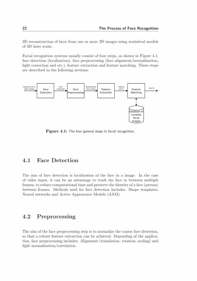
Facial recognition systems usually consist of four steps, as shown in Figure 4.1;face detection (localization), face preprocessing (face alignment/normalization,light correction and etc.), feature extraction and feature matching. These stepsare described in the following sections.
Figure 4.1: The four general steps in facial recognition.
4.1 Face Detection
The aim of face detection is localization of the face in a image. In the caseof video input, it can be an advantage to track the face in between multipleframes, to reduce computational time and preserve the identity of a face (person)between frames. Methods used for face detection includes: Shape templates,Neural networks and Active Appearance Models (AAM).
4.2 Preprocessing
The aim of the face preprocessing step is to normalize the coarse face detection,so that a robust feature extraction can be achieved. Depending of the applica-tion, face preprocessing includes: Alignment (translation, rotation, scaling) andlight normalization/correlation.

4.3 Feature Extraction 23
4.3 Feature Extraction
The aim of feature extraction is to extract a compact set of interpersonal dis-criminating geometrical or/and photometrical features of the face. Methods forfeature extraction include: PCA, FLDA and Locality Preserving Projections(LPP).
4.4 Feature Matching
Feature matching is the actual recognition process. The feature vector obtainedfrom the feature extraction is matched to classes (persons) of facial imagesalready enrolled in a database. The matching algorithms vary from the fairlyobvious Nearest Neighbor to advanced schemes like Neural Networks.
4.5 Thesis Perspective
This thesis will cover all four general areas in face recognition, though the pri-mary focus is on feature extraction and feature matching.
A survey of face detection algorithms is presented in Chapter 7. Preprocessingof facial images is discussed in Chapter 8. A more in-depth description of featureextraction methods is presented in Chapter 9. The performance of these featureextraction methods is presented in Chapter 10, where the Nearest Neighboralgorithm will be used for feature matching. A new face recognition algorithmis developed in Chapter 11.

24 The Process of Face Recognition

Chapter 5
Face Recognition
Considerations
In this chapter general considerations of the process of face recognition arediscussed. These are:
• The variation of facial appearance of different individuals, which can bevery small.
• The non-linear manifold on which face images reside.
• The problem of having a high-dimensional input space and only a smallnumber of samples.
The scope of this thesis is further defined with the respect to these considera-tions.
5.1 Variation in Facial Appearance
A facial image is subject to various factors like facial pose, illumination andfacial expression as well as lens aperture, exposure time and lens aberrations of

26 Face Recognition Considerations
the camera. Due to these factors large variations of facial images of the sameperson can occur. On the other hand, sometimes small interpersonal variationsoccur. Here the extreme is identical twins, as can be seen in Figure 5.1. Differentconstraints in the process of acquiring images can be used to filter out some ofthese factors, as well as use of preprocessing methods.
In a situation where the variation among images obtained from the same personis larger than the variation among images of two individuals persons more com-prehensive data than 2D images must be acquired to do computer based facialrecognition. Here, accurate laser scans or infrared images (showing the bloodvessel distribution in the face) can be used. These methods are out of the scopeof this thesis and will not be discussed further. This thesis is mainly concernedwith 2D frontal face images.
Figure 5.1: Small interpersonal variations illustrated by identical twins.Courtesy of www.digitalwilly.com.
5.2 Face Analysis in an Image Space
When looking at the photometric information of a face, face recognition mostlyrely on analysis of a subspace, since faces in images reside in a submanifold of theimage space. This can be illustrated by an image consisting of 32 × 32 pixels.This image contains a total of 1024 pixels, with the ability to display a longrange of different scenerys. Using only an 8-bit gray scale per pixel this imagecan show a huge number of different configurations, exactly 2561024 = 28192. Asa comparison the world population is only about 232. It is clear that only a smallfraction of these image configurations will display faces. As a result most of the

5.2 Face Analysis in an Image Space 27
original image space representation is very redundant from a facial recognitionpoint of view. It must therefore be possible to reduce the input image spaceto obtain a much smaller subspace, where the objective of the subspace is toremove noise and redundancy while preserving the discriminative informationof the face.
However, the manifolds where faces reside seem to be highly non-linear andnon-convex [5, 53]. The following experiment explores this phenomenon in anattempt to obtain a deeper understanding of the problem.
5.2.1 Exploration of Facial Submanifolds
The purpose of the experiment presented in this section is to visualize that thefacial images reside in a submanifold which is highly non-linear and non-convex.
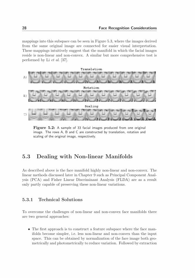
For this purpose ten similar facial images were obtained from three persons ofthe IMM Frontal Face Database1, yielding a total of 30 images. All images wereconverted to grayscale, cropped to only contain the facial region and scaled to100 × 100 pixels. Then 33 new images were produced from each of the originalimages by following manipulations:
• Translation; Translation of the original image was done along the x-axisusing the set (in pixels):
{−30,−24,−18,−12,−6, 0, 6, 12, 18, 24, 30}
• Rotation; Rotation of the original image was done around the center ofthe image using the set (in degrees):
{−10,−8,−6,−4,−2, 0, 2, 4, 6, 8, 10}
• Scaling; Scaling of the original image was done using the set (in %):
{70, 76, 82, 88, 94, 100, 106, 112, 118, 124, 130}
These manipulations resulted in the production of 30 × 33 = 990 images. Anexample of 33 images produced from one original image is shown in Figure 5.2.A Principal Component Analysis was conducted on the original 30 images toproduce a three-dimensional subspace spanned by the three largest principalcomponents. Then all 990 images were mapped into this subspace. These
1This data set is further described in Chapter 6.
28 Face Recognition Considerations
mappings into this subspace can be seen in Figure 5.3, where the images derivedfrom the same original image are connected for easier visual interpretation.These mappings intuitively suggest that the manifold in which the facial imagesreside is non-linear and non-convex. A similar but more comprehensive test isperformed by Li et al. [37].
Figure 5.2: A sample of 33 facial images produced from one originalimage. The rows A, B and C are constructed by translation, rotation andscaling of the original image, respectively.
5.3 Dealing with Non-linear Manifolds
As described above is the face manifold highly non-linear and non-convex. Thelinear methods discussed later in Chapter 9 such as Principal Component Anal-ysis (PCA) and Fisher Linear Discriminant Analysis (FLDA) are as a resultonly partly capable of preserving these non-linear variations.
5.3.1 Technical Solutions
To overcome the challenges of non-linear and non-convex face manifolds thereare two general approaches:
• The first approach is to construct a feature subspace where the face man-ifolds become simpler, i.e. less non-linear and non-convex than the inputspace. This can be obtained by normalization of the face image both geo-metrically and photometrically to reduce variation. Followed by extraction

5.3 Dealing with Non-linear Manifolds 29
Figure 5.3: Results of the exploration of facial submanifolds. The 990images derived from 30 original facial images are mapped into a three-dimensional space spanned by the three largest eigenvectors of the originalimages. The images derived form the original images are connected. Theimages of the three persons are plotted in different colors. The three setsof 30 × 11 images derived by translation, rotation and scaling are displayedin row A, B and C, respectively.

30 Face Recognition Considerations
of features in the normalized image. For this purpose linear methods likePCA, FLDA or even non-linear methods as Kernel Fisher DiscriminantAnalysis (KFDA) can be used [1]. These methods will be described inChapter 9.
• The second approach is to construct classification engines capable of solv-ing the difficult non-linear classification problems of the image space.Methods like Neural Networks, Support Vector Machines etc. can be usedfor this purpose.
In addition the two approaches can be combined.
Work done using only the first approach to statistically understand and simplifythe complex problem of facial recognition is pursued in this thesis.
5.4 High Input Space and Small Sample Size
Another problem associated with face recognition is the high input space of animage and the usually small sample size of an individual. An image consistingof 32 × 32 pixels resides in a 1024-dimensional space, where as the number ofimages of a specific person typically is much smaller. A small number of imagesof a specific person may not be sufficient to make a appropriate approximationof the manifold, which can cause a problem. An illustration of this problemis displayed in Figure 5.4. Currently, no known solution comes to mind forsolving this problem. Other than capturing a sufficient number of samples toapproximate the manifold in a satisfying way.

5.4 High Input Space and Small Sample Size 31
Figure 5.4: An illustration of the problem of not being capable of sat-isfactory approximating the manifold when only having a small number ofsamples. The samples are denoted by circles.

32 Face Recognition Considerations

Chapter 6
Available Data
This chapter presents a small survey of databases used for facial detection andrecognition.
These databases include the IMM Frontal Face Database [21], which has beenrecorded and annotated with landmarks as a part of this thesis. The technicalreport made in conjunction with the IMM Frontal Face Database is found inAppendix A.
Finally, an in-depth description of the actual subsets of three databases used inthis thesis is presented. The three databases used are:
• IMM Frontal Face Database: Used for initial testing in Chapter 10.
• The AR database: Used for a comprehensive test of the MIDM face recog-nition method (which is proposed in Chapter 11). The test results areshown in Chapter 13.
• The XM2VTS database: Used for evaluating the performance of theMIDM algorithm.
Work done using the XM2VTS database has been performed in collaboration
34 Available Data
with Dr. David Delgado Gomez1. The obtained results are to be used for theparticipation in the ICBA20062 Face Verification Contest in Hong Kong, Jan-uary 2006.
6.1 Face Databases
In order to build/train and reliably test face recognition algorithms sizeabledatabases of face images are needed. Many face databases to be used for non-commercial purposes are available on the internet, either free of charge or forsmall fees.
These databases are recorded under various conditions and with various appli-cations in mind. The following sections briefly describe some of the availabledatabases which are widely known and used.
6.1.1 AR
The AR-database was recorded in 1998 at the Computer Vision Center inBarcelona. The database contains images of 116 people; 70 male and 56 fe-male. Every person was recorded in two sessions each consisting of 13 images,resulting in a total of 3016 images. The two sessions were recorded two weeksapart. The 13 images of each session captured varying facial expressions, illumi-nations and occlusions. All images of the AR database are color images with aresolution of 768 × 576 pixels. Landmark annotations based on a 22-landmarkscheme are available for some of the images of the AR database.
Link: “http://rvl1.ecn.purdue.edu/∼aleix/aleix face DB.html”
6.1.2 BioID
The BioID database was recorded in 2001. BioID contains 1521 images of 23persons, about 66 images per person. The database was recorded during anunspecified number of sessions using a high variation of illumination, facialexpression and background. The degree of variation was not controlled resulting
1Post-doctoral at the Computational Imaging Lab, Department of Technology, PompeuFabra University, Barcelona.
2International Conference on Biometrics 2006.

6.1 Face Databases 35
in “real” life image occurrences. All images of the BioID database are recordedin grayscale with a resolution of 384 × 286 pixels. Landmark annotations basedon a 20-landmark scheme are available.
Link: “http://www.humanscan.de/support/downloads/facedb.php”
6.1.3 BANCA
The BANCA multi database was collected as part of the European BANCAproject. BANCA contains images, video and audio samples, though only theimages are described here. BANCA contains images of 52 persons. Every personwas recorded in 12 sessions each consisting of 10 images, resulting in a total of6240 images. The sessions were recorded during a three months period. Threedifferent image qualities were used to acquire the images, where each imagequality was recorded during four sessions. All images are recorded in color witha resolution of 720 × 576 pixels.
Link: “http://www.ee.surrey.ac.uk/banca/”
6.1.4 IMM Face Database
The IMM Face Database was recorded in 2001 at the Department of Informaticsand Mathematical Modelling - Technical University of Denmark. The databasecontains images of 40 people; 33 male and 7 female. It was recorded during onesession and consists of 7 images per person resulting in a total of 240 images.The 7 images of each person were captured under varying facial expressions,camera view points and illuminations. Most of the images are recorded in colorwhile the rest are recorded in grayscale, all with a resolution of 640 × 480 pixels.Landmark annotations based on a 58-landmark scheme are available.
Link: “http://www2.imm.dtu.dk/pubdb/views/publication details.php?id=3160”
6.1.5 IMM Frontal Face Database
The IMM Frontal Face Database was recorded in 2005 at the Department of In-formatics and Mathematical Modelling - Technical University of Denmark. Thedatabase contains images of 12 people; all males. The database was recordedduring one session and consists of 10 images of each person resulting in a total

36 Available Data
of 120 images. The 10 images of each person were captured under varying facialexpressions. All images are recorded in color with a resolution of 2560 × 1920pixels. Landmark annotations based on a 73-landmark scheme are available.
Link: “http://www2.imm.dtu.dk/∼aam/datasets/imm frontal face db high res.zip”
6.1.6 PIE
The Pose, Illumination and Expression (PIE) database was recorded in 2000 atCarnegie Mellon University in Pittsburgh. The database contains images of 68persons all recorded in one session. More than 600 images of each person wereincluded in the database, resulting in a total of 41368 images. The images werecaptured under varying facial expressions, camera view points and illuminations.All images are recorded in color with a resolution of 640 × 468 pixels.
Link: “http://www.ri.cmu.edu/projects/project 418.html”
6.1.7 XM2VTS
The XM2VTS multi database was recorded at the University of Surrey. Thedatabase contains images, video and audio samples, though only the images aredescribed here. XM2VTS contains images of 295 people. Every person wasrecorded during 4 sessions each consisting of four images per person, resultingin a total of 4720 images. The sessions were recorded during a four monthperiod and captured both the frontal and the profiles of the face. All imagesare recorded in color with a resolution of 720 × 576 pixels.
Link: “http://www.ee.surrey.ac.uk/Research/VSSP/xm2vtsdb/”
6.2 Data Sets Used in this Work
Three out of four data set used in this thesis are collected from face databasesand consist of two parts: facial images and landmark annotations of the facialimages. The last data set used in this thesis consists of 3D laser scans of faces.The next sections present the four data sets.
6.2 Data Sets Used in this Work 37
6.2.1 Data Set I
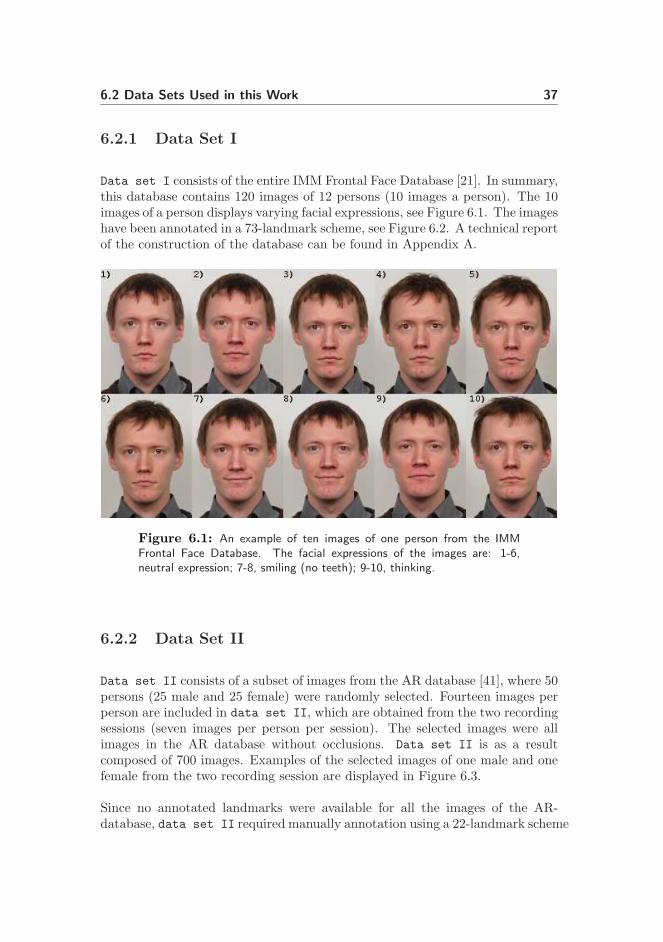
Data set I consists of the entire IMM Frontal Face Database [21]. In summary,this database contains 120 images of 12 persons (10 images a person). The 10images of a person displays varying facial expressions, see Figure 6.1. The imageshave been annotated in a 73-landmark scheme, see Figure 6.2. A technical reportof the construction of the database can be found in Appendix A.
Figure 6.1: An example of ten images of one person from the IMMFrontal Face Database. The facial expressions of the images are: 1-6,neutral expression; 7-8, smiling (no teeth); 9-10, thinking.
6.2.2 Data Set II
Data set II consists of a subset of images from the AR database [41], where 50persons (25 male and 25 female) were randomly selected. Fourteen images perperson are included in data set II, which are obtained from the two recordingsessions (seven images per person per session). The selected images were allimages in the AR database without occlusions. Data set II is as a resultcomposed of 700 images. Examples of the selected images of one male and onefemale from the two recording session are displayed in Figure 6.3.
Since no annotated landmarks were available for all the images of the AR-database, data set II required manually annotation using a 22-landmark scheme

38 Available Data
Figure 6.2: The 73-landmark annotation scheme used on the IMMFrontal Face Database.

6.2 Data Sets Used in this Work 39
Figure 6.3: Examples of 14 images of one female and one male obtainedfrom the AR database. The rows of images (A, B) and (C, D) was capturedduring two different sessions. The columns display: 1, neutral expression;2, smile; 3, anger; 4, scream; 5, left light on; 6, right light on; 7, both sidelights on.
40 Available Data
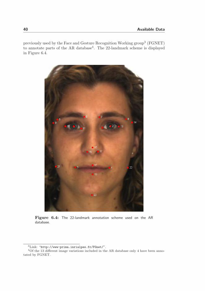
previously used by the Face and Gesture Recognition Working group3 (FGNET)to annotate parts of the AR database4. The 22-landmark scheme is displayedin Figure 6.4.
Figure 6.4: The 22-landmark annotation scheme used on the ARdatabase.
3Link: “http://www-prima.inrialpes.fr/FGnet/”.4Of the 13 different image variations included in the AR database only 4 have been anno-
tated by FGNET.

6.2 Data Sets Used in this Work 41
6.2.3 Data Set III
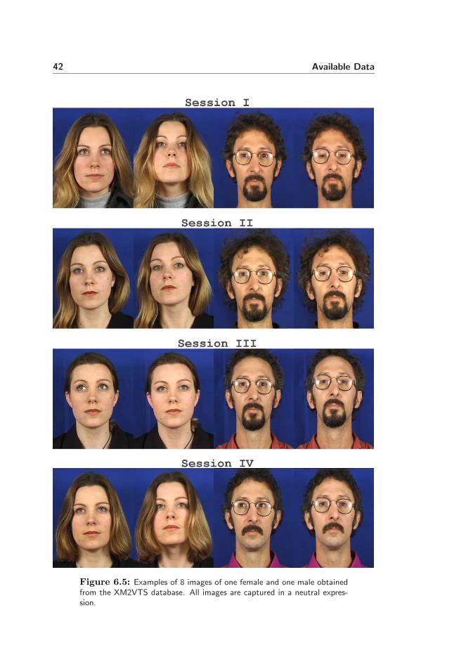
Data set III consists of all the frontal images from the XM2VTS database[43]. To summarize, 8 frontal images were captured of 295 individuals during 4sessions, resulting in data set III consisting of a total of 2360 images. Exam-ples of the selected images of one male and one female from the four recordingsession are displayed in Figure 6.5.
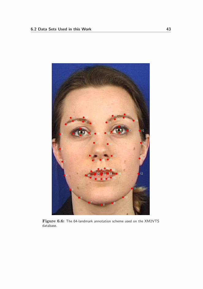
A 68-landmark annotation scheme is available for this data set, made in collabo-ration between the EU FP5 projects UFACE and FGNET. However, this thesisuses two non-public 64-landmark sets. The first set is obtained by manually an-notation, where the second is obtained automatically by an optimized ASM [52].Both landmark sets were created by the Computational Imaging Lab, Depart-ment of Technology, Pompeu Fabra University, Barcelona. The 64-landmarkscheme is displayed in Figure 6.6.
6.2.4 Data Set IV
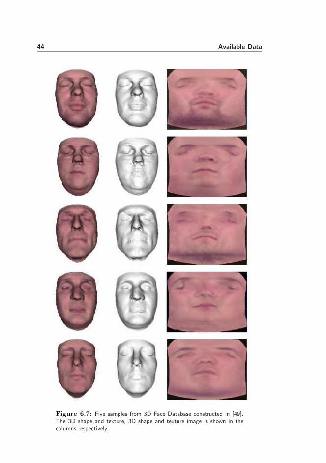
Data set IV consists of the entire 3D Face Database constructed by KarlSkoglund [49] at the Department of Informatics and Mathematical Modelling- Technical University of Denmark. This database includes 24 3D laser scansof 24 individuals (including one baby) and 24 texture images correspondingto the laser scans. Examples of five samples from data set IV are shown inFigure 6.7.
42 Available Data
Figure 6.5: Examples of 8 images of one female and one male obtainedfrom the XM2VTS database. All images are captured in a neutral expres-sion.
6.2 Data Sets Used in this Work 43
Figure 6.6: The 64-landmark annotation scheme used on the XM2VTSdatabase.
44 Available Data
Figure 6.7: Five samples from 3D Face Database constructed in [49].The 3D shape and texture, 3D shape and texture image is shown in thecolumns respectively.

Part II
Assessment


Chapter 7
Face Detection: A Survey
This chapter deals with the problem of face detection. Since the scope of thisthesis is face recognition, this chapter will serve as an introduction to alreadydeveloped algorithms for face detection.
As described earlier in Chapter 4, face detection is the necessary first step in aface recognition system. The purpose of face detection is to localize and extractthe face region from the image background. However, since the human face isa highly dynamic object displaying large degree of variability in appearance,automatic face detection remains a difficult task.
The problem is complicated further by the continually changes over time of thefollowing parameters:
• The three-dimensional position of the face.
• Removable features, such as spectacles and beards.
• Facial expression.
• Partial occlusion of the face, e.g. by hair, scarfs and sunglasses.
• Orientation of the face.

48 Face Detection: A Survey
• Lighting conditions.
The following will distinguish between the two terms face detection and facelocalization.
Definition 7.1 Face detection , the process of detecting all faces (if any) ina given image.
Definition 7.2 Face localization , the process of localizing one face in a givenimage, i.e. the image is assumed to contain one, and only one face.
More than 150 methods for face detection have been developed, though only asmall subset are addressed here. In Yang et al. [60] face detection methods aredivided into four categories:
• Knowledge-based methods: The knowledge-based methods use a setof rules, that describe what to capture. The rules are constructed fromthe intuitive human knowledge of facial components and can be simplerelations among facial features.
• Feature invariant approaches: The aim of feature invariant approachesis to search for structural features, which are invariant to changes in poseand lighting conditions.
• Template matching methods: Template matching methods constructsone or several templates (models) for describing facial features. The cor-relation between an input image and the constructed model(s) enables themethod to discriminate over the case of face or non-face.
• Appearance-based methods: Appearance-based methods use statisti-cal analysis and machine learning to extract the relevant features of a faceto be able to discriminate between face and non-face images. The featuresare composed of both the geometrical information and the photometricinformation.
The knowledge-based methods and the feature invariant approaches are mainlyused only for face localization, where as template matching methods and appear-ance-based methods can be used for face detection as well as face localization.
7.1 Representative Work of Face Detection 49
Approach Representative WorkKnowledge-based
Multiresolution rule-based method [57]Feature invariant
- Facial Features Grouping of edges [36]- Texture Space Gray-Level Dependence matrix of face pat-
tern [14]- Skin Color Mixture of Gaussian [58]- Multiple Features Integration of skin color, size and shape [34]Template matching
- Predefined face templates Shape templates [13]- Deformable Templates Active Shape Models [35]Appearance-based method
- Eigenfaces & Fisherfaces Eigenvector decomposition and clustering [54]- Neural Network1 Ensemble of neural networks and arbitration
schemes [47]- Deformable Models Active Appearance Models [10]
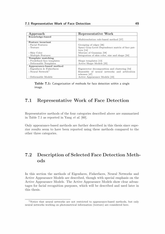
Table 7.1: Categorization of methods for face detection within a singleimage.
7.1 Representative Work of Face Detection
Representative methods of the four categories described above are summarizedin Table 7.1 as reported in Yang et al. [60].
Only appearance-based methods are further described in this thesis since supe-rior results seem to have been reported using these methods compared to theother three categories.
7.2 Description of Selected Face Detection Meth-ods
In this section the methods of Eigenfaces, Fisherfaces, Neural Networks andActive Appearance Models are described, though with special emphasis on theActive Appearance Models. The Active Appearance Models show clear advan-tages for facial recognition purposes, which will be described and used later inthis thesis.
1Notice that neural networks are not restricted to appearance-based methods, but onlyneural networks working on photometrical information (texture) are considered here.
50 Face Detection: A Survey
7.2.1 General Aspects of Face Detections Algorithms
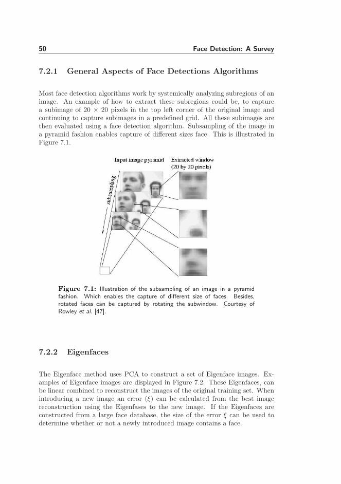
Most face detection algorithms work by systemically analyzing subregions of animage. An example of how to extract these subregions could be, to capturea subimage of 20 × 20 pixels in the top left corner of the original image andcontinuing to capture subimages in a predefined grid. All these subimages arethen evaluated using a face detection algorithm. Subsampling of the image ina pyramid fashion enables capture of different sizes face. This is illustrated inFigure 7.1.
Figure 7.1: Illustration of the subsampling of an image in a pyramidfashion. Which enables the capture of different size of faces. Besides,rotated faces can be captured by rotating the subwindow. Courtesy ofRowley et al. [47].
7.2.2 Eigenfaces
The Eigenface method uses PCA to construct a set of Eigenface images. Ex-amples of Eigenface images are displayed in Figure 7.2. These Eigenfaces, canbe linear combined to reconstruct the images of the original training set. Whenintroducing a new image an error (ξ) can be calculated from the best imagereconstruction using the Eigenfases to the new image. If the Eigenfaces areconstructed from a large face database, the size of the error ξ can be used todetermine whether or not a newly introduced image contains a face.

7.2 Description of Selected Face Detection Methods 51
Figure 7.2: Example of 10 Eigenfaces. Notice that Eigenface no. 10contains much noise and that the Eigenfaces are constructed from the shapefree images described in Section 7.2.5.
Another more robust way is to look upon the subspace2 provided by the eigen-faces, and cluster face images and non-face images in this subspace [54].
7.2.3 Fisherfaces
Much like Eigenfaces, Fisherfaces construct a subspace in which the algorithmcan discriminate between facial and non-facial images. A more in-depth descrip-tion of FLDA, which is used by Fisherfaces, can be found in Chapter 9.
7.2.4 Neural Networks
In a neural network approach features from an image are extracted and fed toa neural network. One huge drawback of neural networks is that they can beextensively tuned, in terms of deciding learning methods and on the number oflayers, nodes, etc.
One of the most significant work in neural network face detection has been doneby Rowley et al. [47, 48]. He used a neural network to classify images in a [−1; 1]range, where -1 and 1 denotes a non-face image and a face image, respectively.Every image window of 20×20 pixels was divided into four 10×10 pixels, 16 5×5pixels and six 20 × 5 pixels (overlapping) sub windows. A hidden node in the
2Principal Component Analysis can reduce the dimensionality of the data, described furtherin Chapter 9.

52 Face Detection: A Survey
neural network was fed each of these sub windows, yielding a total of 26 hiddennodes. A diagram of the neural network design by Rowley et al. [47] is shownin Figure 7.3. The neural network can be improved by adding an extra neuralnetwork to determining the rotation of an image window. This will enable thesystem to capture faces not vertically aligned in the input image, see Figure 7.4.
7.2.5 Active Appearance Models
Active Appearance Models (AAM) are a generalization of the widely used ActiveShape Models (ASM). Instead of only representing the information near edges,an AAM statistically models all texture and shape information inside the targetmodel (here faces) boundary.
To build an AAM a training set has to be provided, which contains images andlandmark annotations of facial features.
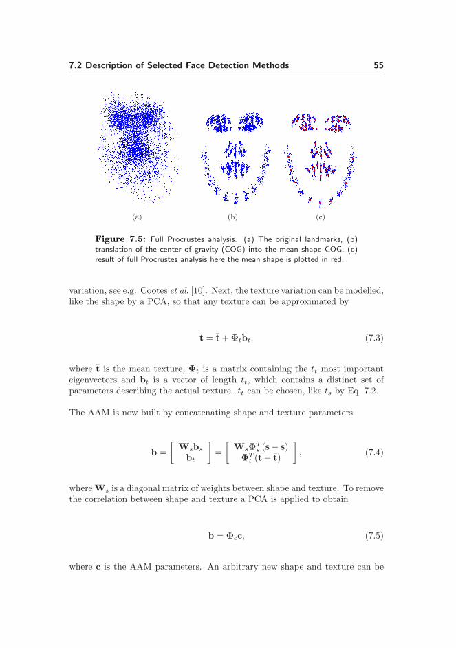
The first step in building an AAM is to align the landmarks using a Procrustesanalysis [28], as displayed in Figure 7.5. Next the shape variation is modelledby a PCA, so that any shape can be approximated by
s = s + Φsbs, (7.1)
where s is the mean shape, Φs is a matrix containing the ts most importanteigenvectors and bs is a vector of length ts, which contains a distinct set ofparameters describing the actual shape. The number ts of eigenvectors in Φs andthe length of bs is chosen so that the model represents a user-defined proportionof the total variance in data. To obtain the proportion of p percent variance thevalue of ts can be chosen by
ts∑
i=1
λi =>p
100
n∑
i=1
λi, (7.2)
where λi is the eigenvalue corresponding to the ith eigenvector and n is the totalnumber of non-zero eigenvalues.
The texture variation is modelled by first removing shape information by warp-ing all face images onto the mean shape. This is called the set of shape freeimages. Several methods can then be applied to eliminate global illumination

7.2 Description of Selected Face Detection Methods 53
Figure 7.3: Diagram of the neural network developed by Rowley et al.[47].

54 Face Detection: A Survey
Figure 7.4: Diagram displaying an improved version of the neural networkin Figure 7.3. Courtesy of Rowley et al. [48].
7.2 Description of Selected Face Detection Methods 55
(a) (b) (c)
Figure 7.5: Full Procrustes analysis. (a) The original landmarks, (b)translation of the center of gravity (COG) into the mean shape COG, (c)result of full Procrustes analysis here the mean shape is plotted in red.
variation, see e.g. Cootes et al. [10]. Next, the texture variation can be modelled,like the shape by a PCA, so that any texture can be approximated by
t = t + Φtbt, (7.3)
where t is the mean texture, Φt is a matrix containing the tt most importanteigenvectors and bt is a vector of length tt, which contains a distinct set ofparameters describing the actual texture. tt can be chosen, like ts by Eq. 7.2.
The AAM is now built by concatenating shape and texture parameters
b =
[
Wsbs
bt
]
=
[
WsΦTs (s − s)
ΦTt (t − t)
]
, (7.4)
where Ws is a diagonal matrix of weights between shape and texture. To removethe correlation between shape and texture a PCA is applied to obtain
b = Φcc, (7.5)
where c is the AAM parameters. An arbitrary new shape and texture can be

56 Face Detection: A Survey
generated by
s = s + ΦsW−1s Φc,sc (7.6)
and
t = t + ΦtΦc,tc, (7.7)
where
Φc =
[
Φc,s
Φc,t
]
. (7.8)
The process of placing the AAM mean shape and texture on a specific locationin an image and search for a face near by this location, is shown in Figure 7.6.This process will not be described further here. For a more detailed descrip-tion of AAM the paper Cootes et al. [10] or the master thesis by Mikkel BilleStegmann [50] are recommended.
One advantage of the AAM (and ASM) algorithm compared to other face detec-tion algorithms is that a localized face is described both by shape and texture.
Thus, a well defined shape of the face can be obtained by an AMM. This isan improvement from others face detection algorithms, where the result is asub image containing a face without knowing exactly which pixels representbackground and which represent the face. An AAM is also desirable for trackingin video sequences, assuming that changes are minimal from frame to frame.Due to these advantages an AAM is used as the face detection algorithm in thisthesis, when automatic detection is required.

7.2 Description of Selected Face Detection Methods 57
Figure 7.6: Face detection (approximations) obtained by AAM, whenthe model is initialized close to the face. The first column is the meanshape and texture of the AAM. The last column is the converged shapeand texture of the AAM. Courtesy Cootes et al. [10].

58 Face Detection: A Survey
Chapter 8
Preprocessing of a Face Image
The face preprocessing step aims at normalizing, i.e. reducing the variation ofimages obtained during the face detection step. Using AAM in the process offace detection provides a well defined framework to retrieve the photometricinformation as a shape free image as well as the geometric information as ashape. Since this already has been described previously in this thesis only thesubject of light correction will be described within this chapter.
8.1 Light Correction
As described in Section 3.2, unpredictable change in lighting conditions is aproblem in facial recognition. Therefore, it is desirable to normalize the photo-metric information in terms of light correction to optimize the facial recognition.Here, two light correction methods are described.
8.1.1 Histogram Equalization
Histogram equalization (HE) can be used as a simple but very robust way toobtain light correction when applied to small regions such as faces. The aim of
60 Preprocessing of a Face Image
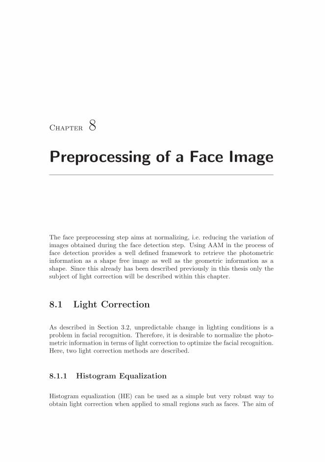
HE is to maximize the contrast of an input image, resulting in a histogram of theoutput image which is as close to a uniform histogram as possible. However, thisdoes not remove the effect of a strong light source but maximizes the entropy ofan image, thus reducing the effect of differences in illumination within the same“setup” of light sources. By doing so, HE makes facial recognition a somehowsimpler task. Two examples of HE of images can be seen in Figure 8.1. Thealgorithm of HE is straight forward and will not be explained here, an interestedreader can obtain the algorithm in Finlayson et al. [22].
Image before
Image after
0 100 2000
100
200
300
400
500
600Histogram
Pixel intensity
Fre
quen
cy
0 100 2000
100
200
300
400
500
600Histogram
Pixel intensity
Fre
quen
cy
Image before
Image after
0 100 2000
100
200
300
400
500
600Histogram
Pixel intensity
Fre
quen
cy
0 100 2000
100
200
300
400
500
600Histogram
Pixel intensity
Fre
quen
cy
Figure 8.1: Examples of histogram equalization used upon two images toobtain standardized images with maximum entropy. Notice, only the facialregion of an image is used in the histogram equalization.
8.1.2 Removal of Specific Light Sources based on 2D FaceModels
The removal of specific light sources based on 2D face models [56] is anothermethod to obtain light correlation of images. The method creates a pixelwisecorrespondence of images (as already described in Section 7.2.5, the AAM shapefree image). By doing so, the effect of illumination upon each pixel x = {x, y}of an image can be expressed by the equation
Fx = ai,x · Fx + bi,x, (8.1)

8.1 Light Correction 61
where F and F are the images of the same scene recoded at normal lightingcondition (diffuse lighting) and upon the influence of a specific light source(illumination mode i), respectively. ai,x is the multiplication compensation,and bi,x is the additive compensation of the illumination mode i of pixel x in
the image F.
Having n sets of images in the normal illumination and the mode i illumination,Eq. 8.1 can be rewritten as
G = G
[
ai,x
bi,x
]
, (8.2)
where
G =
F1,x
...
Fn,x
, G =
F1,x 1...
...Fn,x 1
. (8.3)
If the n sets of images are of different persons, then the rows of G and G areindependent and the least-squares solution to ai,x and bi,x in Eq. 8.2 is
[
ai,x
bi,x
]
= (GT G)−1GT G. (8.4)
Using Eq. 8.4 upon every pixel in the shape free image, the illumination com-pensation images Ai and Bi can be constructed. By doing so it is possibleto reconstruct a face image in normal lighting conditions from a face image inlighting condition i by
Fx =Fx − bi,x
ai,x
. (8.5)
Different schemes can be used to identify the lighting condition of a specific faceimage, in Xie et al. [56] a FLDA is used.
Removal of two specific illumination conditions is displayed in Figure 8.2. Thisused the illumination compensation maps displayed in Figure 8.4. However, this

62 Preprocessing of a Face Image
method sometimes creates artifacts in the faces. A close-up of the illuminationcorrected faces from Figure 8.2 can be seen in Figure 8.3 that displays this fact.
Figure 8.2: Removal of specific illumination conditions from facial im-ages. A) shows the facial images in normal diffuse lighting. B) column1-4 and 5-8 show facial images captured under right and left illumination,respectively. C) is the compensated images.
Figure 8.3: A close-up of the faces reconstructed in Figure 8.2. Noticethat faces 1-4 are influenced only little by artifacts while faces 5-8 areinfluenced substantially by artifacts.
8.2 Discussion
It is clear that HE is a good and robust way of normalizing images. The morecomplex method of removing specific illumination conditions seems to yieldimpressive results, but has the drawback of sometimes imposing artifacts ontothe images, as can be seen in Figure 8.3, where “shadows of spectacles” canbe seen on persons not wearing spectacles. It was decided to only preprocess

8.2 Discussion 63
Figure 8.4: Illumination compensation maps used for removal of specificillumination conditions. Rows A) and B) display the illumination compen-sation maps for facial images captured under left and right illumination,respectively.

64 Preprocessing of a Face Image
facial images with HE to ensure that the images are independent. No testswere performed to see how facial recognition performs under the influence ofthe artifacts introduced by the removal of specific light sources based on 2Dface models. This will be saved for future work.

Chapter 9
Face Feature Extraction:
Dimensionality Reduction
Methods
Table 9.1 lists the most promising dimensionality reduction methods (featureextraction methods) used for face recognition. Out of these Principal Compo-nent Analysis, Fisher Linear Discriminant Analysis, Kernel Fisher Linear Dis-criminant Analysis and Locality Preserving Projections will be described in thefollowing.
Preserving Technique Method
Global Structure
LinearFisher Linear Discriminant Analysis
Principal Component Analysis
Non-linearKernel Fisher Linear Discriminant Analysis
Kernel Principal Component Analysis
Local Structure
Linear Locality Preserving Projections
Non-linearIsomap
Laplacian Eigenmap
Table 9.1: Dimensionality reduction methods.
66 Face Feature Extraction: Dimensionality Reduction Methods
9.1 Principal Component Analysis
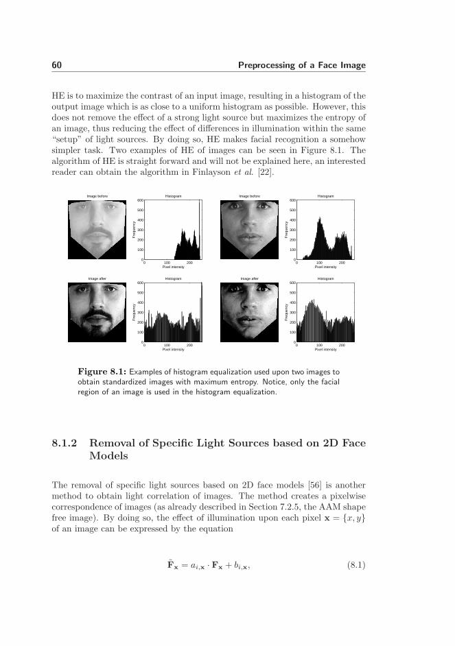
Principal Component Analysis (PCA), also known as Karhunen-Loeve transfor-mation, is a linear transformation which captures the variance of the input data.The coordinate system in which the data resides is rotated by PCA, so that thefirst-axis is parallel to the highest variance in the data (in a one-dimension pro-jection). The remaining axes can be explained one at the time as being parallelto the highest variance of the data, while all axes are constrained to be orthogo-nal to all previous found axes. To summarize, the first-axis will contain highestvariance, the second-axis contain the second highest variance, etc. An exam-ple in two dimensions is shown in Figure 9.1. PCA, which is an unsupervisedmethod, is a powerful tool for data analysis, especially if data resides in a spacehigher than three dimensions, where graphical representations are hard. One ofthe main applications of PCA is dimension reduction, with little or no loss ofdata variation. This is used to remove redundancy and compress data.
Figure 9.1: An example of PCA in two dimensions, showing the PCAaxis that maximizes the variation in the first principal component: PCA 1.
9.1.1 PCA Algorithm
Different methods can be used to calculate the PCA basis vectors. Here eigenval-ues and eigenvectors of the covariance matrix of the data are used. Considering

9.1 Principal Component Analysis 67
the data
X = [x1,x2, · · · ,xn], (9.1)
where n is the amount of data samples, xi is the ith data sample of dimensiond. First is the mean of X subtracted from the data
X = [x1 − x,x2 − x, · · · ,xn − x]. (9.2)
The covariance matrix ΣX is calculated by
ΣX =1
nXXT . (9.3)
The principal axes are now given by the eigenvectors ΦX of the covariancematrix
ΣXΦX = ΦXΛX, (9.4)
where
ΛX =
λ1 0 · · · 0
0 λ2. . .
......
. . .. . . 0
0 · · · 0 λd
(9.5)
is the diagonal matrix of eigenvalues corresponding to the eigenvectors of
ΦX = [φ1,φ2, · · · ,φd]. (9.6)
The eigenvector corresponding to the highest eigenvalue represents the basisvector containing the most data variance, i.e. the first principal component.

68 Face Feature Extraction: Dimensionality Reduction Methods
The ith data sample, xi, can be transformed into the PCA space by
yi = Φ−1
X(xi − x) = ΦT
X(xi − x). (9.7)
Notice that an orthogonal matrix as ΦX has the property Φ−1
X= ΦT
X. Data in
the PCA space can be transformed back into the original space by
xi = ΦXyi + x. (9.8)
If only a subset of the eigenvectors in ΦX is selected, then this will result indata being projected into a PCA subspace. This can be very useful to reduceredundancy in the data, i.e. remove all eigenvectors equal to zero. The abovemethod is described in greater detail in Ersbøll et al. [19].
9.1.2 Computational Issues of PCA
If one has n data samples in a d high-dimensional space where n ≪ d. Thenthe computational time is quite large for retrieving eigenvectors and eigenvaluesfrom the d×d covariance matrix. The time needed for eigenvector decompositionincreases by the cube of the covariance matrix size [10]. However, it is possibleto calculate the eigenvectors of the non-zero eigenvalues from a much smallermatrix with size n × n, by use of
Σn =1
nXT X, (9.9)
where X is calculated by Eq. 9.2. The non-zero eigenvalues of the matrices inEq. 9.4 and Eq. 9.9 are equal
Λn = ΛX. (9.10)
The eigenvectors corresponding to non-zero eigenvalues can be expressed as
ΦX = XΦn. (9.11)

9.2 Fisher Linear Discriminant Analysis 69
Notice that these eigenvectors are not normalized. This can be proved by theEckhart-Young Theorem [50].
9.2 Fisher Linear Discriminant Analysis
Fisher Linear Discriminant Analysis (FLDA), also known as Canonical Discrim-inant Analysis is like PCA, a linear transformation. Unlike PCA, FLDA is asupervised method, which implies that all training-data samples must be as-sociated (manually) with a class. FLDA maximizes the between-class varianceas well as minimizes the within-class variance. A graphic example of FLDA isshown in Figure 9.2.
Figure 9.2: An example of FLDA in two dimensions, showing the FLDAaxis that maximizes the separation between the classes and minimizes thevariation inside the classes.
The objective function for FLDA is as follows
maxw
wT SBw
wT SW w, (9.12)

70 Face Feature Extraction: Dimensionality Reduction Methods
where the between-matrix is defined as
SB =
c∑
i=1
ni(xi − x)(xi − x)T (9.13)
and the within-matrix as
SW =c
∑
i=1
ni∑
j=1
(xi,j − xi)(xi,j − xi)T , (9.14)
where xi,j is the jth sample in class i, xi mean of class i, x mean of all samples,c is number of classes and ni is the number of samples in class i.
The optimal projection that maximizes the between-class variance and min-imizes the within-class variance is given by the direction of the eigenvectorassociated to the maximum eigenvalue of S−1
W SB . Notice that the number ofnon-zero eigenvalues is at most number of classes minus one [4].
9.2.1 FLDA in Face Recognition Problems
In face recognition problems SW is nearly always singular. This is due to thefact that the rank of SW is at most n − c, where n (the number of trainingsamples) usually is much smaller than the number of pixels in each image.
In order to overcome this problem a PCA is usually performed1 on the imagesprior to FLDA, which removes redundancy and makes the data samples morecompact. The within-matrix, SW , is made non-singular by only considering thef most important principal components from the PCA, where f is the numberof non-zero eigenvalues of the within-matrix SW .
9.3 Locality Preserving Projections
The Locality Preserving Projections (LPP) algorithm has recently been de-veloped [29]. When high-dimensional data lies on a low dimension manifold
1Normally capturing between 95-99% of the variance.
9.3 Locality Preserving Projections 71
embedded in the data space, then LPP approximate the eigenfunctions of theLaplace-Beltrami operator of the manifold. LPP aims at preserving the localstructure of the data. This is unlike PCA and FLDA, which aims at preservingthe global structure of the data.
LPP is unsupervised and performs a linear transformation. It models the man-ifold structure by constructing an adjacency graph, which is a graph expressinglocal nearness of the data. This is highly desirable for face recognition comparedto non-linear local structure preserving methods in Table 9.1, since it is signifi-cantly less computationally expensive and more importantly it is defined in allpoints and not just in the training points as Isomaps and Laplacian Eigenmaps.
The objective function of LPP is
min∑
ij
(yi − yj)2Sij , (9.15)
where yi is a one-dimensional representation of the data sample xi and Sij isan entry in the similarity matrix S that represent the adjacency graph. Theadjacency graph weight α if notes i and j are connected can be chosen by:
• A parameter function, [t ∈ R], e.g.
α = e−‖xi−xj‖2
t . (9.16)
• A constant, e.g.
α = 1. (9.17)
Two ways of constructing the adjacency graph is:
• ǫ-neighborhood, [ǫ ∈ R]:
Sij =
{
α, ‖xi − xj‖2 < ǫ0 otherwise
(9.18)
• k nearest neighbors, [k ∈ N]:
Sij =
α, if xi is among the k nearest neighbors of xj orxj is among the k nearest neighbors of xi
0 otherwise(9.19)

72 Face Feature Extraction: Dimensionality Reduction Methods
The similarity matrix will inflict heavy penalties on the objective function inEq. 9.15 if neighboring points xi and xj are mapped far apart in the outputspace. By minimizing the objective function LPP tries to ensure that yi andyj are close in the output space if xi and xj are close in the input space. Theobjective function can be reduced to
arg minw
= wT XLXT w subject to wT XDXT w = 1, (9.20)
where the constraint wT XDXT w = 1 is used to normalize w, by
12
∑
ij(yi − yj)2sij m
12
∑
ij(wT xi − wT xj)
2sij m∑
ij wT xisijxTi w −
∑
ij wT xisijxTj w m
∑
i wT xidiix
Ti w − wT XSXT w m
wT XDXT w − wT XSXT w mwT X(D − S)XT w m
wT XLXT w
, (9.21)
where X is a matrix containing all data points [x1,x2, . . . ,xn], D is a diagonalmatrix where the elements is Dii =
∑
j sji and L = D − S is the Laplacian
matrix. To normalize w the system is constrained by wT XDXT w = 1.
The vector w, which minimizes the objective function, is given by the eigenvectorcorresponding to the minimum eigenvalue solution of the generalized eigenvalueproblem
XLXT w = λXDXT w. (9.22)
If XDXT has full rank it reduces the eigenvalue problem to
(XDXT )−1XLXT w = λw. (9.23)
Let W = [w0,w1, . . . ,wn−1] be the solutions to Eq. 9.23 ordered according tothe eigenvalues, λ0 < λ1 < · · · < λn−1. Then the LPP projection can then be
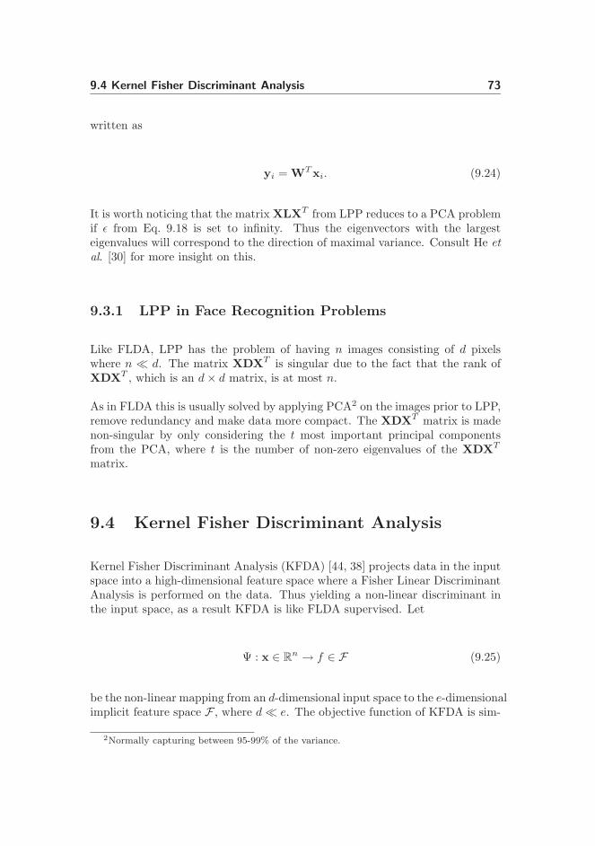
9.4 Kernel Fisher Discriminant Analysis 73
written as
yi = WT xi. (9.24)
It is worth noticing that the matrix XLXT from LPP reduces to a PCA problemif ǫ from Eq. 9.18 is set to infinity. Thus the eigenvectors with the largesteigenvalues will correspond to the direction of maximal variance. Consult He etal. [30] for more insight on this.
9.3.1 LPP in Face Recognition Problems
Like FLDA, LPP has the problem of having n images consisting of d pixelswhere n ≪ d. The matrix XDXT is singular due to the fact that the rank ofXDXT , which is an d × d matrix, is at most n.
As in FLDA this is usually solved by applying PCA2 on the images prior to LPP,remove redundancy and make data more compact. The XDXT matrix is madenon-singular by only considering the t most important principal componentsfrom the PCA, where t is the number of non-zero eigenvalues of the XDXT
matrix.
9.4 Kernel Fisher Discriminant Analysis
Kernel Fisher Discriminant Analysis (KFDA) [44, 38] projects data in the inputspace into a high-dimensional feature space where a Fisher Linear DiscriminantAnalysis is performed on the data. Thus yielding a non-linear discriminant inthe input space, as a result KFDA is like FLDA supervised. Let
Ψ : x ∈ Rn → f ∈ F (9.25)
be the non-linear mapping from an d-dimensional input space to the e-dimensionalimplicit feature space F , where d ≪ e. The objective function of KFDA is sim-
2Normally capturing between 95-99% of the variance.

74 Face Feature Extraction: Dimensionality Reduction Methods
ilar to Eq. 9.12 of FLDA
maxw
wT SΨBw
wT SΨW w
, (9.26)
where w ∈ F and the between- and within-matrices of F are
SΨB =
1
c(c − 1)
c∑
i=1
c∑
j=1
(ui − uj)(ui − uj)T (9.27)
and
SΨW =
1
c
c∑
i=1
1
ni
ni∑
j=1
(Ψ(xj) − ui)(Ψ(xj) − ui)T , (9.28)
where c is the number of classes, ni is the number of samples in class i and ui
denotes the mean of the samples in class i in F given by
ui =1
ni
ni∑
j=1
Ψ(xj). (9.29)
When the dimensionality of F becomes very high (or even infinite), this problembecomes impossible to solve. However, by using the kernel trick [2] it is notnecessary to compute Ψ explicitly. The kernel trick uses Mercer kernels tocompute the inner product of two vectors in a feature space, L, by using onlythe vectors of the input space, K(x,y) = Ψ(x) ·Ψ(y). A Mercer kernel satisfiesthe Mercer conditions:
• K is continuous.
• K is symmetrical, K(x,y) = K(y,x).
• K is positive semi-definite. That is for any set of vectors{x1,x2, . . . ,xm} belonging to the input space, the matrixM = (K(xi,xj))ij , {i, j} = 1, . . . ,m is positive semi-definite.

9.4 Kernel Fisher Discriminant Analysis 75
The kernel trick states that any kernel K(x,y) satisfying the Mercer conditionscan be expressed as a dot product in a high-dimensional space. Two examplesin the Mercer kernels family are Gaussian kernels,
K(xi,xj) = e−‖x−y‖2
t , t ∈ R+ (9.30)
and polynomial kernels,
K(xi,xj) = (x · y)d, d ∈ R+. (9.31)
In order to avoid computing Ψ explicitly, Eq. 9.26 to Eq. 9.28 have to be for-mulated using only inner products of Ψ, i.e. Ψ(x) ·Ψ(y), which can be replacedby a kernel function.
Any solution w ∈ F must lie in the span of all training samples in F , proof ofthis can be obtained by consulting a reproducing kernels textbook. Thereforethere exist n coefficients αi so that an expansion of w can be written as
w =n
∑
i=1
αiΨ(xi). (9.32)
By use of Eq. 9.29 and Eq. 9.32 the projection of each class mean ui into w canbe written as
wT ui = αT
1ni
∑ni
j=1 K(x1,xj)1ni
∑ni
j=1 K(x2,xj)...
1ni
∑ni
j=1 K(xn,xj)
= αT mi. (9.33)
Now, by use of Eq. 9.27 and Eq. 9.33 the numerator of Eq. 9.26 can be formulatedas
αT KBα, (9.34)

76 Face Feature Extraction: Dimensionality Reduction Methods
where
KB =1
c(c − 1)
c∑
i=1
c∑
j=1
(mi − mj)(mi − mj)T . (9.35)
Similarly, by use of Eq. 9.28, Eq. 9.29 and Eq. 9.32 the denominator of Eq. 9.26can be formulated as
αT KW α, (9.36)
where
KW =1
c
c∑
i=1
1
ni
ni∑
j=1
(ζj − mi)(ζj − mi)T (9.37)
and
ζj = [K(x1,xj) K(x2,xj) · · · K(xn,xj)]T . (9.38)
Eq. 9.26 can be rewritten using Eq. 9.34 and Eq. 9.36 yielding
maxα
αT KBα
αT KW α. (9.39)
FLDA can now be performed implicit in F by calculating the leading eigenvec-tors of K−1
W KB in the input space. The projection of a given point x into w inF is given by
w · Ψ(x) =
n∑
i=1
αiK(xi,x). (9.40)

9.4 Kernel Fisher Discriminant Analysis 77
9.4.1 Problems of KFDA
KFDA has numerical problems since KW is seldom of full rank. A simple wayto avoid this is to add a multiple of the identity matrix to KW [44] so that
KW = KW + µI. (9.41)
Another problem is how to select a kernel function for different tasks, which isstill an open problem [38].

78 Face Feature Extraction: Dimensionality Reduction Methods

Chapter 10
Experimental Results I
The purpose of this chapter is to evaluate the the four feature extraction meth-ods described in Chapter 9. To summarize, the four extraction methods are:
• Principal Component Analysis
• Locality Preserving Projections
• Fisher Linear Discriminant Analysis
• Kernel Fisher Discriminant Analysis
The idea is to extract facial features from facial images by use of the fourmethods mentioned above presuming that the facial features are easily separatedin the feature space. For the tests presented in this chapter data set I is used.The tests are divided into two parts, where the first is an illustration of the fourfeature spaces, while the second tests face identification using a nearest neighborclassifier in the four output spaces. The choice of nearest neighbor algorithm asclassifier used in the second part is based on the following observations:
• It is very simple, yet powerful if it contains an adequate number of classi-fied samples, resulting in well defined populations.

80 Experimental Results I
• It does not need training.
• It produces reproducible results, i.e. if several tests are conducted usingthe same protocol for testing the obtained results are unambiguous. Incontrast, neural networks use some degree of randomness in the training,which in some cases results in non-reproducible results.
Eq. 9.17 (α = 1) is used in these tests as the entries in the LPP’s similaritymatrix and it is constructed according to Eq. 9.19 (the k nearest neighbors).After careful consideration k = ⌊m/2⌋ was used, since this seems to yield thebest results. Here, m is the average number of samples in the training set ofa specific person. For KFDA the Gaussian kernel in Eq. 9.30 is used, wheret = 250000 was used, since this seemed to yield the best results.
10.1 Illustration of the Feature Spaces
In the following sections feature spaces of PCA, LPP, FLDA and KFDA areillustrated by scatter plot matrices of the three most discriminative dimensions.Data set I consisting of 120 images of 12 persons was divided into two groupsof 60 images each. The first group consists of the images {1, 3, 5, 7, 9} of eachperson1 and is used to calculate the mapping between the image space and thefeature space. The second group consists of the images {2, 4, 6, 8, 10}. These aremapped into the feature spaces to visualize the separability of the 12 personswhen using the four methods. Furthermore, the test was conducted to obtain acombined projection of photometric and geometric information. Tests could beconducted only concerning either the photometric or the geometric information,but due to space constraints these tests were not included.
The PCA space is constructed like a AAM (described in Section 7.2.5). Firsta PCA is performed on the shape free images and then on the shapes. Theobtained results were then combined and a third PCA was performed yieldinga subspace containing both the geometric and photometric information. Whencombining the results obtained from the first two PCA’s the weighting betweentexture and shape is one (i.e. Ws = I in the AAM terminology) and the variancecaptured by the PCA accounts for 99.9%. The PCA scatter plot matrix obtainedin the test is displayed in Figure 10.1.
The LPP, FLDA and KFDA spaces are constructed in the compact PCA spacedescribed above. This is done to avoid singularity problems (described in Chap-ter 9) and to reduce the huge workload associated with the image space of
1The image numbers are described in the technical rapport in Appendix A.

10.1 Illustration of the Feature Spaces 81
−100 −50 0 50 100−100
−50
0
50
100
φ 1
φ 1
−100 −50 0 50 100−80
−60
−40
−20
0
20
40
60
φ 2
φ 1
−100 −50 0 50 100−30
−20
−10
0
10
20
30
φ 3
φ 1
−100 −50 0 50 100−100
−50
0
50
100
φ 1
φ 2
−100 −50 0 50 100−80
−60
−40
−20
0
20
40
60
φ 2
φ 2
−100 −50 0 50 100−30
−20
−10
0
10
20
30
φ 3
φ 2
−30 −20 −10 0 10 20 30−100
−50
0
50
100
φ 1
φ 3
−30 −20 −10 0 10 20 30−80
−60
−40
−20
0
20
40
60
φ 2
φ 3
−30 −20 −10 0 10 20 30−30
−20
−10
0
10
20
30
φ 3
φ 3
Figure 10.1: The PCA scatter plot matrix of the combined features fromdata set I. The 12 persons of data set I are displayed by different colorsand symbols.

82 Experimental Results I
KFDA. The LPP, FLDA and KFDA scatter plot matrices are displayed in Fig-ure 10.2, Figure 10.3 and Figure 10.4, respectively.
−60 −40 −20 0 20 40−60
−40
−20
0
20
40
φ 1
φ 1
−60 −40 −20 0 20 40−20
−15
−10
−5
0
5
10
15
20
φ 2
φ 1
−60 −40 −20 0 20 40−60
−40
−20
0
20
40
φ 3
φ 1
−20 −10 0 10 20−60
−40
−20
0
20
40
φ 1
φ 2
−20 −10 0 10 20−20
−15
−10
−5
0
5
10
15
20
φ 2
φ 2
−20 −10 0 10 20−60
−40
−20
0
20
40
φ 3
φ 2
−60 −40 −20 0 20 40−60
−40
−20
0
20
40
φ 1
φ 3
−60 −40 −20 0 20 40−20
−15
−10
−5
0
5
10
15
20
φ 2
φ 3
−60 −40 −20 0 20 40−60
−40
−20
0
20
40
φ 3
φ 3
Figure 10.2: The LPP scatter plot matrix of the combined features fromdata set I. The 12 persons of data set I are displayed by different colorsand symbols.

10.1 Illustration of the Feature Spaces 83
−40 −20 0 20 40−40
−30
−20
−10
0
10
20
30
40
φ 1
φ 1
−40 −20 0 20 40−60
−40
−20
0
20
40
60
φ 2
φ 1
−40 −20 0 20 40−40
−20
0
20
40
60
φ 3
φ 1
−60 −40 −20 0 20 40 60−40
−30
−20
−10
0
10
20
30
40
φ 1
φ 2
−60 −40 −20 0 20 40 60−60
−40
−20
0
20
40
60
φ 2
φ 2
−60 −40 −20 0 20 40 60−40
−20
0
20
40
60
φ 3
φ 2
−40 −20 0 20 40 60−40
−30
−20
−10
0
10
20
30
40
φ 1
φ 3
−40 −20 0 20 40 60−60
−40
−20
0
20
40
60
φ 2
φ 3
−40 −20 0 20 40 60−40
−20
0
20
40
60
φ 3
φ 3
Figure 10.3: The FLDA scatter plot matrix of the combined featuresfrom data set I. The 12 persons of data set I are displayed by differentcolors and symbols.
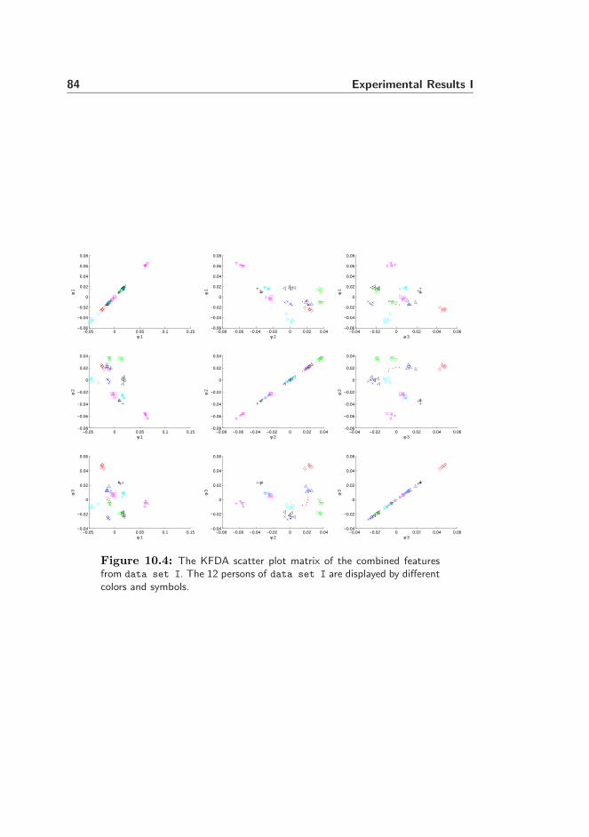
84 Experimental Results I
−0.05 0 0.05 0.1 0.15−0.06
−0.04
−0.02
0
0.02
0.04
0.06
0.08
φ 1
φ 1
−0.05 0 0.05 0.1 0.15−0.08
−0.06
−0.04
−0.02
0
0.02
0.04
φ 2
φ 1
−0.05 0 0.05 0.1 0.15−0.04
−0.02
0
0.02
0.04
0.06
φ 3
φ 1
−0.08 −0.06 −0.04 −0.02 0 0.02 0.04−0.06
−0.04
−0.02
0
0.02
0.04
0.06
0.08
φ 1
φ 2
−0.08 −0.06 −0.04 −0.02 0 0.02 0.04−0.08
−0.06
−0.04
−0.02
0
0.02
0.04
φ 2
φ 2
−0.08 −0.06 −0.04 −0.02 0 0.02 0.04−0.04
−0.02
0
0.02
0.04
0.06
φ 3
φ 2
−0.04 −0.02 0 0.02 0.04 0.06−0.06
−0.04
−0.02
0
0.02
0.04
0.06
0.08
φ 1
φ 3
−0.04 −0.02 0 0.02 0.04 0.06−0.08
−0.06
−0.04
−0.02
0
0.02
0.04
φ 2
φ 3
−0.04 −0.02 0 0.02 0.04 0.06−0.04
−0.02
0
0.02
0.04
0.06
φ 3
φ 3
Figure 10.4: The KFDA scatter plot matrix of the combined featuresfrom data set I. The 12 persons of data set I are displayed by differentcolors and symbols.
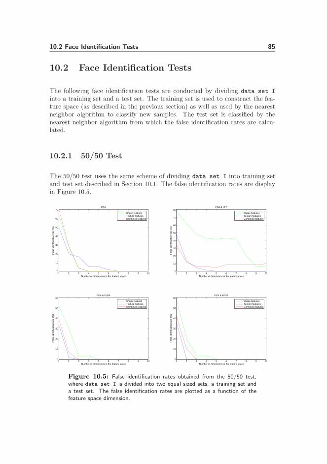
10.2 Face Identification Tests 85
10.2 Face Identification Tests
The following face identification tests are conducted by dividing data set I
into a training set and a test set. The training set is used to construct the fea-ture space (as described in the previous section) as well as used by the nearestneighbor algorithm to classify new samples. The test set is classified by thenearest neighbor algorithm from which the false identification rates are calcu-lated.
10.2.1 50/50 Test
The 50/50 test uses the same scheme of dividing data set I into training setand test set described in Section 10.1. The false identification rates are displayin Figure 10.5.
1 2 3 4 5 6 7 8 9 100
10
20
30
40
50
60
70PCA
Number of dimensions in the feature space
Fal
se id
entif
icat
ion
rate
(%
)
Shape featuresTexture featuresCombined features
1 2 3 4 5 6 7 8 9 100
10
20
30
40
50
60
70
80PCA & LPP
Number of dimensions in the feature space
Fal
se id
entif
icat
ion
rate
(%
)
Shape featuresTexture featuresCombined features
1 2 3 4 5 6 7 8 9 100
10
20
30
40
50
60PCA & FLDA
Number of dimensions in the feature space
Fal
se id
entif
icat
ion
rate
(%
)
Shape featuresTexture featuresCombined features
1 2 3 4 5 6 7 8 9 100
10
20
30
40
50
60PCA & KFDA
Number of dimensions in the feature space
Fal
se id
entif
icat
ion
rate
(%
)
Shape featuresTexture featuresCombined features
Figure 10.5: False identification rates obtained from the 50/50 test,where data set I is divided into two equal sized sets, a training set anda test set. The false identification rates are plotted as a function of thefeature space dimension.

86 Experimental Results I
10.2.2 Ten-fold Cross-validation Test
In the ten-fold cross-validation test data set I is divided into ten folds, eachfold consisting of one image of all persons. The cross-validation test was per-formed at each of the ten iterations by using nine folds as the training set whileusing the remaining fold as test set. The false identification rates are display inFigure 10.6.
1 2 3 4 5 6 7 8 9 100
10
20
30
40
50
60
70
80PCA
Number of dimensions in the feature space
Fal
se id
entif
icat
ion
rate
(%
)
Shape featuresTexture featuresCombined features
1 2 3 4 5 6 7 8 9 100
10
20
30
40
50
60
70
80PCA & LPP
Number of dimensions in the feature space
Fal
se id
entif
icat
ion
rate
(%
)
Shape featuresTexture featuresCombined features
1 2 3 4 5 6 7 8 9 100
10
20
30
40
50
60PCA & FLDA
Number of dimensions in the feature space
Fal
se id
entif
icat
ion
rate
(%
)
Shape featuresTexture featuresCombined features
1 2 3 4 5 6 7 8 9 100
5
10
15
20
25
30
35
40
45
50PCA & KFDA
Number of dimensions in the feature space
Fal
se id
entif
icat
ion
rate
(%
)
Shape featuresTexture featuresCombined features
Figure 10.6: The false identification rates obtained from the ten-foldcross-validation test. The false identification rates are plotted as a functionof the feature space dimension.

10.3 Discussion 87
10.3 Discussion
Analysis of the scatter plot matrices, displayed in Figure 10.1, Figure 10.2,Figure 10.3 and Figure 10.4 indicate that the methods LPP, FLDA and KFDAimprove the separability of the classes (persons) compared to PCA. Though,LPP seems to have a problem separating two of the classes. This is supportedby the LPP FIR graphs (in Figure 10.5 and Figure 10.6) where the combinedfeature shows a general FIR of 10%. In addition the shape feature display avery high percentage of FIR in an interval of 10 to 80%.
These problems with the shape and combined features displayed by LPP areprobably due to the way the similarity matrix is constructed. In the current im-plementation the nearness in the input space is defined by Euclidean distances,which is not necessarily a meaningful measurement of a shape.
When using KFDA one has to consider the choice of a kernel function resultingin a satisfying result. This choice is as described earlier still an open problem.The parameter t in the chosen kernel function used in the presented tests has tobe adjusted when the KFDA method is used on a new data set. Another problemwhen using KFDA compared to linear methods is the higher risk of overfittingthe training data, which in turn causes a drop in performance. KFDA as aresult can be considered “too flexible” from an implementation point of view.
Analysis of the FIR graphs shows that FLDA performs nearly as well as KFDA.FLDA, in contrast to LPP and KFDA, does not contain any parameters needinginitializing, which makes FLDA a very robust method. Therefore, the designof a new face recognition algorithm presented in the next chapter is built onFLDA.
The problem of improving the similarity matrix in LPP is not pursued furtherin this thesis.
The overall results show that the variation of data set I is very small.

88 Experimental Results I

Part III
Development


Chapter 11
Multiple Individual
Discriminative Models
Typically, the techniques PCA, LPP, FLDA and KFDA are in the literatureclassified with a nearest neighbor algorithm [40, 29, 44].
However, some inconvenience appears when testing the techniques using un-known persons in the test set. In this case, a criterium has to be chosen todecide whether or not an image of an specific person belongs to the trainingset, e.g. only people with a Euclidean distance less than a given threshold areconsidered as part of the training set. However, such a threshold should notnecessarily be the same for all classes (persons). The estimation of differentthresholds is not straightforward. Additional data are needed to estimate these.In addition, it is a problem to determine the optimal dimensionality of the fourtechniques described above.
In this chapter, a novel technique is proposed that addresses the inconveniencesdescribed above. In this technique, denoted Multiple Individual DiscriminativeModels (MIDM), the data are projected by FLDA into c one-dimensional spacesinstead of the “normal” FLDA (c−1)-dimensional space. Here, c is the numberof people in the data set.
The aim of each of the individual models, obtained by the projection of thetraining set into the c one-dimensional spaces, is to characterize a given person

92 Multiple Individual Discriminative Models
uniquely, resulting in each of the individual models representing one person.The multiple one-dimensional models allow statistical interpretation of the “de-gree of membership” of a given person and allows detection of unknown persons(faces). Furthermore, these individual models have several advantages in in-terpretability, characterization, accuracy and easiness in updating one or moremodels belonging to the MIDM.
11.1 Algorithm Description
The proposed algorithm is composed of two steps. The first step builds anindividual model for each person in the database using the photometrical andgeometrical information provided by the available images. Each model charac-terizes a given person and discriminates the person from the other people in thedatabase. The second step carries out the identification. A classifier, which isrelated to the standard Gaussian distribution, decides whether or not a facialimage belongs to a person in the database. In this section, the two steps ofthe algorithm are described in detail. A diagram of the algorithm is displayedin Figure 11.1. This diagram will be referred to during the description of thealgorithm to allow the reader to gain a deeper understanding.
11.1.1 Creations of the Individual Models
11.1.1.1 Obtaining the Geometry of the Face
The geometrical characterization of a given face is obtained by means of thetheory of statistical shape analysis [18]. In this theory, objects (faces) are rep-resented by shapes.
Definition 11.1 A shape is, according to Kendall [33], all the geometrical in-formation that remains when location, scale and rotational effects are filteredout from an object.
In order to describe a shape, a set of landmarks or points of correspondencematching between and within populations are placed on each face.
To obtain a shape representation according to the Definition 11.1, the obtainedlandmarks are aligned in order to remove the location, rotational and scaling ef-fects. To achieve this goal, the 2D Procrustes analysis is carried out (Figure 11.1A).
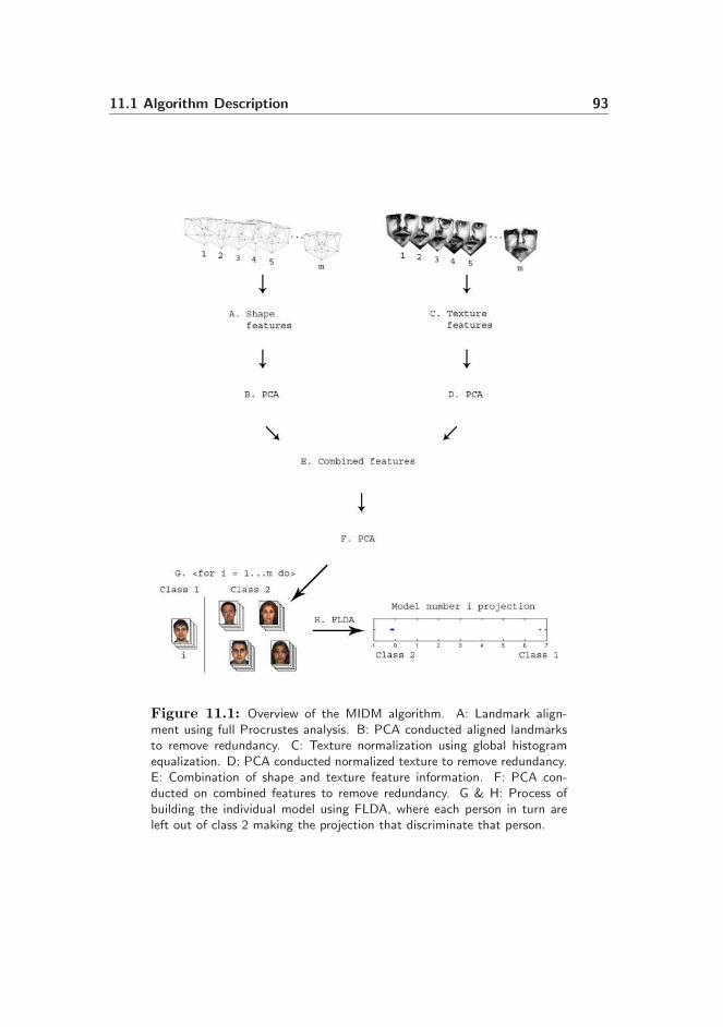
11.1 Algorithm Description 93
Figure 11.1: Overview of the MIDM algorithm. A: Landmark align-ment using full Procrustes analysis. B: PCA conducted aligned landmarksto remove redundancy. C: Texture normalization using global histogramequalization. D: PCA conducted normalized texture to remove redundancy.E: Combination of shape and texture feature information. F: PCA con-ducted on combined features to remove redundancy. G & H: Process ofbuilding the individual model using FLDA, where each person in turn areleft out of class 2 making the projection that discriminate that person.
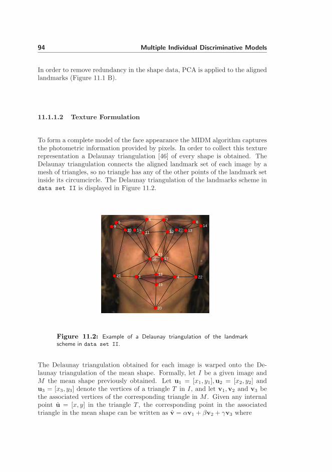
94 Multiple Individual Discriminative Models
In order to remove redundancy in the shape data, PCA is applied to the alignedlandmarks (Figure 11.1 B).
11.1.1.2 Texture Formulation
To form a complete model of the face appearance the MIDM algorithm capturesthe photometric information provided by pixels. In order to collect this texturerepresentation a Delaunay triangulation [46] of every shape is obtained. TheDelaunay triangulation connects the aligned landmark set of each image by amesh of triangles, so no triangle has any of the other points of the landmark setinside its circumcircle. The Delaunay triangulation of the landmarks scheme indata set II is displayed in Figure 11.2.
1 2
3 4
56 7 8
910
11 12 1314
1516 17
18
19
20
21 22
Figure 11.2: Example of a Delaunay triangulation of the landmarkscheme in data set II.
The Delaunay triangulation obtained for each image is warped onto the De-launay triangulation of the mean shape. Formally, let I be a given image andM the mean shape previously obtained. Let u1 = [x1, y1],u2 = [x2, y2] andu3 = [x3, y3] denote the vertices of a triangle T in I, and let v1,v2 and v3 bethe associated vertices of the corresponding triangle in M . Given any internalpoint u = [x, y] in the triangle T , the corresponding point in the associatedtriangle in the mean shape can be written as v = αv1 + βv2 + γv3 where

11.1 Algorithm Description 95
α = 1 − (β + γ), (11.1)
β =yx3 − x1y − x3y1 − y3x + x1y3 + xy1
−x2y3 + x2y1 + x1y3 + x3y2 − x3y1 − x1y2, (11.2)
γ =xy2 − xy1 − x1y2 − x2y + x2y1 + x1y
−x2y3 + x2y1 + x1y3 + x3y2 − x3y1 − x1y2. (11.3)
This transformation extracts the same shape free image of a given face image asproduced by AAM in Section 7.2.5. A histogram equalization is applied to thecollected texture as described in Section 8.1.1 to reduce the effects of illumina-tion differences. This histogram equalization is performed independently in eachof the three color channels (RGB) to reduce lightning artifacts. Afterwards, thethree color channels can be converted into gray scale if a more compact repre-sentation is desirable (Figure 11.1 C). PCA is conducted on the texture datato reduce dimensionality and data redundancy (Figure 11.1 D). The solutionto the memory problems due to the huge dimension of the covariance matrix issolved as described in Section 9.1.2.
11.1.1.3 Combining Color and Geometry
The shape and texture features are combined in a matrix (Figure 11.1 E). Inorder to remove correlation between shape and texture and to make the datarepresentation more compact a third PCA is performed on the combined shapeand texture matrix (Figure 11.1 F).
11.1.1.4 Building an Individual Model
Once the geometrical and photometrical information of the faces has been cap-tured, the MIDM algorithm builds an individual model for each person in thetraining set. Each individual model is built in two steps. First the trainingset is divided into two groups, one representing a person i and one representingpersons other than i (Figure 11.1 G). Second FLDA is applied on the two groups(Figure 11.1 H). This is repeated for every person in the training set, resultingin individual models representing each person.
96 Multiple Individual Discriminative Models
11.1.2 Classification
In order to obtain a method to classify a given image, the different individualmodels are first standardized. The standardization of model i = 1, . . . ,m isbased on two assumptions. First, the number of observations for person i ismuch smaller than the number of the observations for all other people. Secondthe projection of the other people follows a Gaussian distribution. The twoassumptions imply that the distribution of all the observations can be assumedas a Gaussian distribution with outliers. The standardization of model i is thenachieved by transforming the projections into a standard Gaussian distribution,keeping the projections of the person i positive. Formally, let xi be the mean ofthe projections on model i, σi the standard deviation and xi,j the projection ofimage j in model i. These projections are standardized by
xi,j = (xi,j − xi)/σi. (11.4)
If the standardized projections of the images corresponding to person i arenegative, then xi,j are replaced by −xi,j for all projections. This causes theprojections of the images corresponding to person i to be positive and far fromthe mean of the Gaussian distribution.
Once the model i is standardized, the probability that a projected image belongsto the person i is given by the value of the standard normal cumulative functionin the projected value. This is used to classify a given image. If it is assumed thatthe image belongs to a person from the training set, the image is projected byall the individual models of MIDM. The image is then classified as belonging tothe model that results in the largest probability. Furthermore, it is statisticallypossible to decide whether or not a given person belongs to the training set.This can be achieved by comparing the largest projection obtained in all themodels with a threshold. E.g. if a probability of 99.9% is required, a given imagewill only be considered as belonging to the database, if the projection in oneof the individual models is higher than 3.1 standard deviations. This in turnestimates the FAR to be 0.1%. It is not possible to estimate the FRR this way.The estimation of FRR, like other classifiers, requires use of test data set.
11.2 Discussion
The MIDM technique is very robust and highly accurate (as shown later inthis thesis) and it is based on a very simple setup analyzing single 2D images.Furthermore, the projected subspaces yield a very intuitive interpretation, i.e.

11.2 Discussion 97
a high projected value indicates a large probability of that image belonging tothe person that the model represents. The statistical classifier does not needtraining. Instead the value of the threshold can be selected to achieve a desiredFAR, i.e. the FAR is 1−P(t) where P is the cumulative distribution function ofthe standard normal distribution and t is the threshold in standard deviations.However, it is possible to train the classifier if e.g. the optimal separation of theimposter and the client classes is of interest (EER threshold). The performanceof MIDM is extensively reported in Chapter 13.

98 Multiple Individual Discriminative Models

Chapter 12
Reconstruction of 3D Face
from a 2D Image
In order to achieve better results in the face recognition process, face recognitionin three dimensions would be interesting, since the face is a three-dimensionalobject. 3D data can be collected in various ways, as already described in Chap-ter 4. However, using the knowledge of statistical shape analysis it could be veryinteresting to investigate the extraction of 3D information from a 2D image usingprior knowledge of faces in 3D.
This chapter will consult this issue, using only frontal facial images. Sincethe topic is on the edge of the scope of this thesis it will not be a conclusivepresentation of the area, but only a brief appetizer.
12.1 Algorithm Description
Extraction of the 3D information from a 2D image is based on the existence of astatistical shape model of 3D faces, i.e. a Point Distribution Model (PDM) [11].By use of PDM the information obtained from a 2D image of a face can be usedto reconstruct the third image dimension, by manipulating the PDM until anoptimal fit is achieved. The fit is calculated by projecting the already annotated
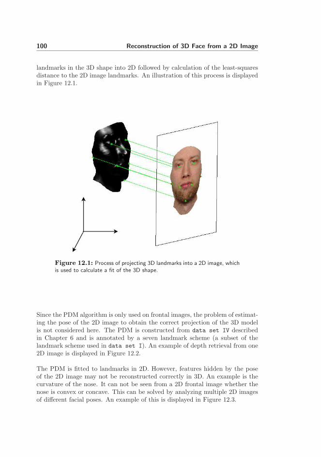
100 Reconstruction of 3D Face from a 2D Image
landmarks in the 3D shape into 2D followed by calculation of the least-squaresdistance to the 2D image landmarks. An illustration of this process is displayedin Figure 12.1.
Figure 12.1: Process of projecting 3D landmarks into a 2D image, whichis used to calculate a fit of the 3D shape.
Since the PDM algorithm is only used on frontal images, the problem of estimat-ing the pose of the 2D image to obtain the correct projection of the 3D modelis not considered here. The PDM is constructed from data set IV describedin Chapter 6 and is annotated by a seven landmark scheme (a subset of thelandmark scheme used in data set I). An example of depth retrieval from one2D image is displayed in Figure 12.2.
The PDM is fitted to landmarks in 2D. However, features hidden by the poseof the 2D image may not be reconstructed correctly in 3D. An example is thecurvature of the nose. It can not be seen from a 2D frontal image whether thenose is convex or concave. This can be solved by analyzing multiple 2D imagesof different facial poses. An example of this is displayed in Figure 12.3.
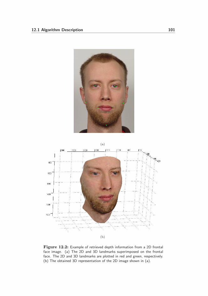
12.1 Algorithm Description 101
(a)
(b)
Figure 12.2: Example of retrieved depth information from a 2D frontalface image. (a) The 2D and 3D landmarks superimposed on the frontalface. The 2D and 3D landmarks are plotted in red and green, respectively.(b) The obtained 3D representation of the 2D image shown in (a).
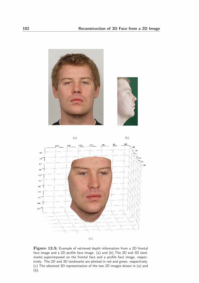
102 Reconstruction of 3D Face from a 2D Image
(a) (b)
(c)
Figure 12.3: Example of retrieved depth information from a 2D frontalface image and a 2D profile face image. (a) and (b) The 2D and 3D land-marks superimposed on the frontal face and a profile face image, respec-tively. The 2D and 3D landmarks are plotted in red and green, respectively.(c) The obtained 3D representation of the two 2D images shown in (a) and(b).

12.2 Discussion 103
12.2 Discussion
No testing was performed to analyze how much the recognition is improved byreconstructing a 3D image from a 2D image. Data set IV only contains 24individuals, and as a result it does not contain enough variation to capture newfaces differently from the images of data set IV. However, the reconstructionsperformed are very promising, and 3D reconstruction is definitely an area ofinterest when performing future work on face recognition.

104 Reconstruction of 3D Face from a 2D Image

Chapter 13
Experimental Results II
13.1 Overview
In this chapter an evaluation of the MIDM algorithm proposed in Chapter 11is performed. The evaluation is divided into two parts as described in thefollowing:
13.1.1 Initial Evaluation Tests
The initial evaluation will be done by performing the following tests on theMIDM algorithm using data set II:
• Identification test. This test will show the performance of MIDMagainst a regular Fisherface with a nearest neighbor classifier. In addition,this experiment aims at testing whether or not the shape information isimportant to the recognition process.
• Verification test. In this test a 25-fold cross-validation scheme is usedto ascertain the FAR and FRR for data set II of the MIDM.
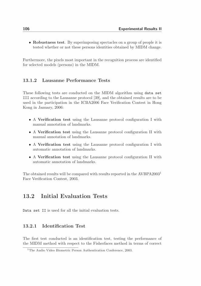
106 Experimental Results II
• Robustness test. By superimposing spectacles on a group of people it istested whether or not these persons identities obtained by MIDM change.
Furthermore, the pixels most important in the recognition process are identifiedfor selected models (persons) in the MIDM.
13.1.2 Lausanne Performance Tests
These following tests are conducted on the MIDM algorithm using data set
III according to the Lausanne protocol [39], and the obtained results are to beused in the participation in the ICBA2006 Face Verification Contest in HongKong in January, 2006:
• A Verification test using the Lausanne protocol configuration I withmanual annotation of landmarks.
• A Verification test using the Lausanne protocol configuration II withmanual annotation of landmarks.
• A Verification test using the Lausanne protocol configuration I withautomatic annotation of landmarks.
• A Verification test using the Lausanne protocol configuration II withautomatic annotation of landmarks.
The obtained results will be compared with results reported in the AVBPA20031
Face Verification Contest, 2003.
13.2 Initial Evaluation Tests
Data set II is used for all the initial evaluation tests.
13.2.1 Identification Test
The first test conducted is an identification test, testing the performance ofthe MIDM method with respect to the Fisherfaces method in terms of correct
1The Audio Video Biometric Person Authentication Conference, 2003.

13.2 Initial Evaluation Tests 107
classification rates.
In order to evaluate the importance of the geometrical information, the Fisher-face technique was modified by replacing the texture data with the shape data.In addition, the shape data and the texture data were combined. The two mod-ified techniques are referred to as Fishershape and Fishercombined from nowon. In addition, the three Fisher-methods are implemented using the shape freeimages instead of normal images, which are generally used by Fisherfaces. Thiswill make the tests more compatible, as they use the same data.
The Euclidean Nearest Neighbor algorithm was used as classifier in the Fishermethods. The MIDM method classified images as belonging to the model yield-ing the highest probability of recognition as described in Section 11.1.2.
The images from data set II were divided into two sets. Images from the firstsession were used to build the individual models, and images from the secondsession were subsequently used to test the performance.
The MIDM method was built using the geometrical (shape), the photometrical(texture) and the combined information of each face corresponding to Fisher-shape, Fisherface and Fishercombined, respectively.
The test was repeated exchanging the roles of the training and test sets, i.e.images from session two was used as training set and images from session oneas test set. The correct identification rates from using the different techniquesare shown in Table 13.1.
The MIDM method shows a higher rate of performance than the Fisher methods(Table 13.1). Moreover, by analyzing the obtained results in Table 13.1 it isindicated that by use of texture data one obtains a higher accuracy than by usingshape data. This implies that the information contained in the texture data ismore significant than the information included in the shape data. However, theinformation contained in the shape data is not insignificant, since the highestcorrect classification rate is obtained when combining both shape and texture.
The importance of geometrical information in facial recognition can be furthersubstantiated by retrieving the shape free image of a person from data set I
who has a very slim face. When looking at the normal image and the shape freeimage displayed in Figure 13.1 even humans can have difficulties determiningwhether or not the two images are of the same person. Though, the differencebetween an shape and the mean shape is not always as significant as displayed
2Number of misclassified images reported in parentheses.3The Fisher-methods are modified to use shape free images.

108 Experimental Results II
Method Input features Correct Identification Rate2
MIDM method Shape 86.4% (95)MIDM method Texture 99.6% (3)MIDM method Texture and Shape 99.9% (1)Fishershape3 Shape 85.9% (99)Fisherface3 Texture 96.9% (22)
Fishercombined3 Texture and Shape 97.1% (20)
Table 13.1: Correct identification rates.
in Figure 13.1.
(a) (b)
Figure 13.1: Importance of geometrical information. (a) the facial regionof an image in data set I, (b) the facial region from (a) displayed as ashape free image (warped into the meanshape).
13.2.2 The Important Image Regions
An interesting property of the MIDM algorithm is that it is capable of deter-mining the most discriminative features of a given person. To illustrate this,four models were built using only the texture information. The pixels of thefaces corresponding to these models are displayed in Figure 13.2. Here the 10%,15% and 25% pixels of the weights of highest value are displayed in red. Byanalyzing Figure 13.2 it is clear that the most important discriminating featuresinclude eyes, noses, spectacles, moles and beards. Notice that the MIDM algo-rithm detects the spectacles and the two moles of person 43 as discriminatingfeatures.

13.2 Initial Evaluation Tests 109
Person nr: 3 10% 15% 25%
Person nr: 16 10% 15% 25%
Person nr: 31 10% 15% 25%
Person nr: 43 10% 15% 25%
Figure 13.2: The 10%, 15% and 25% pixels weights of highest valuemost important for discrimination between the test persons of data set
II. The mentioned pixels are shown in red.

110 Experimental Results II
13.2.3 Verification Test
A verification test was performed to verify whether or not the MIDM algorithmcan be incorporated into a biometrical facial recognition scheme, i.e. whether ornot MIDM can identify people of the training set as well as detecting unknownpeople.
A 25-fold cross-validation scheme was conducted in order to evaluate the per-formance of MIDM. Seven face images of one male and seven face images ofone female of data set II were left out in each cross-validation iteration, i.e.images of 48 people were used in the training of the MIDM algorithm. Just tosummarize, a total of seven images per person were included in the training set.The “left out” male and female were considered as imposters (unknowns).
The verification test was conducted in two scenarios:
• Best case scenario.In the best case scenario the imposter is obligated to try out all knownidentities in the training set in the attempt to be recognized by the MIDM.This is necessary since the imposters in the best case scenario does notknow which person in the training set he/she resembles most. The 25-foldcross-validation results in 8400 client validations (25 folds × 48 persons ×7 images) and 16800 imposter validations (25 folds × 2 persons × 48 totalnumber of identities × 7 images).
• Worst case scenario.In the worst case scenario the imposters do know which person in thetraining set they reassemble most. The imposters will therefore attemptto be recognized by the MIDM only using this identity. In this scenariothe 25-fold cross-validation results in 8400 client validations (25 folds ×48 persons × 7 images) and 350 imposter validations (25 folds × 2 persons× 7 images).
The average False Acceptance Rate (FAR) and average False Rejection Rate(FRR) graphs obtained in the best and worst case scenarios as well as the corre-sponding average Receiver Operating Characteristic curve (ROC) are displayedin Figure 13.3.
The verification test shows a high degree of separability between the client andimposter populations for both scenarios. The highest degree of separation occursat the Equal Error Rate, yielding FAR and FRR at 0.3% and 1.8% obtained forthe best and worst case scenario, respectively.
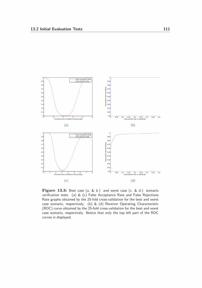
13.2 Initial Evaluation Tests 111
−2 0 2 4 6 80
0.1
0.2
0.3
0.4
0.5
0.6
0.7
0.8
0.9
1
Threshold score (Confidence interval (std))
False Acceptance RateFalse Rejection Rate
(a)
0 0.05 0.1 0.15 0.2 0.25 0.3 0.35 0.40.9
0.91
0.92
0.93
0.94
0.95
0.96
0.97
0.98
0.99
1
False positive rate (1−specificity)
Tru
e po
sitiv
e ra
te (
sens
itivi
ty)
(b)
0 1 2 3 4 5 6 7 80
0.1
0.2
0.3
0.4
0.5
0.6
0.7
0.8
0.9
1
Threshold score (Confidence interval (std))
False Acceptance RateFalse Rejection Rate
(c)
0 0.05 0.1 0.15 0.2 0.25 0.3 0.35 0.40.9
0.91
0.92
0.93
0.94
0.95
0.96
0.97
0.98
0.99
1
False positive rate (1−specificity)
Tru
e po
sitiv
e ra
te (
sens
itivi
ty)
(d)
Figure 13.3: Best case (a. & b.) and worst case (c. & d.) scenarioverification tests. (a) & (c) False Acceptance Rate and False RejectionsRate graphs obtained by the 25-fold cross-validation for the best and worstcase scenario, respectively. (b) & (d) Receiver Operating Characteristic(ROC) curve obtained by the 25-fold cross-validation for the best and worstcase scenario, respectively. Notice that only the top left part of the ROCcurves is displayed.

112 Experimental Results II
In addition, if the algorithm belongs to a security scheme, the degree of accessi-bility can be changed by increasing or decreasing the threshold of the classifier,e.g. if a false rejection rate of 5.5% is allowed in the worst case scenario a 0% falseacceptance rate is obtained. This accommodates biometrical security systemsrequiring a high level of access control.
13.2.4 Robustness Test
Finally, a test is conducted in order to estimate the robustness of the MIDMmethod. In addition, the test aims at settling that the MIDM method not onlydiscriminates on removable features, such as spectacles, but uses permanentfacial features in the discrimination process, as well. To achieve this goal eightpeople (four male and four female) are synthetically fitted with four differenttypes of spectacles. The spectacles were obtained from people belonging to data
set II. By fitting the eight people with the four types of spectacles 32 syntheticimages was obtained.
The test was conducted in two steps.
• First, all images in session of data set II, except for images of the eightselected persons, were used to build the MIDM. The goal is to examinewhether or not the eight selected people are considered as belonging to thetraining set. The results show that none of the 32 synthetic images aremisclassified when considering a threshold of 3.1 standard deviations i.e.the FAR will approximately be 0.1%. This is displayed in Figure 13.4 II,where the projections of one of the eight unknown people into the differentmodels of the MIDM are displayed. The figure shows, that when thedisplayed person is unknown to the MIDM, projections of this person ontothe individual models in the MIDM are all under the selected threshold of3.1. As a result the MIDM does not classify any of the unknown peopleas belonging to the training set.
• Second, the eight people not included in the training set in step one arenow included in the process of building the individuals models. Though,only images of the eight people without spectacles are included. The goalis to analyze whether or not MIDM still is capable of recognizing peopleas belonging to the training set when slight changes in their appearancehave occurred. Here, slight changes in appearance of the eight people aremodelled by the 32 synthetic images. The 32 synthetic images of the eightpersons were classified correctly by the MIDM method. In Figure 13.4 IIIthis is observed for one of the eight persons, where the projections ontothe individual model of this person clearly surpass the threshold of 3.1.

13.3 Lausanne Performance Tests 113
Session Shot Clients Impostors
11 Training set (Clients)2 Evaluation set (Clients)
21 Training set (Clients)2 Evaluation set (Clients) Evaluation set Test set
31 Training set (Clients) (Imposters) (Imposters)2 Evaluation set (Clients)
41
Test set (Clients)2
Table 13.2: Partitioning of data set III according to the Lausanneprotocol configuration I.
In addition, the projections of the person fitted with spectacles into theindividual models of the spectacle owners do not change noteworthily.
Similar results were obtained for all eight people selected to wear spectaclesas seen in Figure 13.4. These results show that MIDM is a highly suitablecandidate to be incorporated into a biometrical security system.
13.3 Lausanne Performance Tests
The Lausanne protocol Luettin et al. [39] describes how to test the XM2VTSfacial database (data set III), to obtain results which can be compared toresults obtained by other methods.
The Lausanne protocol uses two configurations to divide the 295 individualsof data set III into three groups consisting of 200 clients, 25 evaluation im-posters and 70 testing imposters, respectively. The client group is further di-vided into three groups consisting of training clients, evaluation clients andtesting clients, respectively. The five groups are denoted training set (trainingclients), evaluation set (evaluation clients + imposters) and test set (test clients+ imposters) in the following. The partitioning are listed in Table 13.2 andTable 13.3 for the Lausanne protocol configuration I and II, respectively.
The performance tests are conducted by training the MIDM method using thetraining set. The threshold for the classifier was selected as the value at the EERfor the evaluation set. The FAR and FRR of the test set were then calculatedusing this threshold.

114 Experimental Results II
Figure 13.4: Effect of change in a persons appearance, illustrated bysuperimposing spectacles onto a person from data set II not wearingspectacles. (I) Original facial image without spectacles followed by fourimages fitted with four types of spectacles. (II) The corresponding projec-tions into the MIDM models obtained where the person is unknown to theMIDM. (III) The corresponding projections into the MIDM models obtainedwhere the person is known to the MIDM. The red columns in the plots (II& III) represents the model of the person from which the spectacles usedto superimpose were extracted.

13.3 Lausanne Performance Tests 115
Session Shot Clients Impostors
11
Training set (Clients)2
212 Evaluation set Test set
31
Evaluation set (Clients)(Imposters) (Imposters)
2
41
Test set (Clients)2
Table 13.3: Partitioning of data set III according to the Lausanneprotocol configuration II.
13.3.1 Participants in the Face Verification Contest, 2003
The participants in the Face Verification Contest, 2003 originated from seveninstitutions around the world:
• University of Surrey, UK (UniS).
• University of Kent, UK (UniK).
• The Dalle Molle Institute for Perceptual Artificial Intelligence, Switzerland(IDIAP).
• Universite Catholique de Louvain, Belgium (UCL).
• Mahanakron University of Technology, Thailand (MUT).
• Universidad Politcnica de Valencia, Spain (UPV).
• Tubitak Bilten, Turkey (TB).
In the following section results obtained from the MIDM are compared to theresults obtained during the Face Verification Contest, 2003.
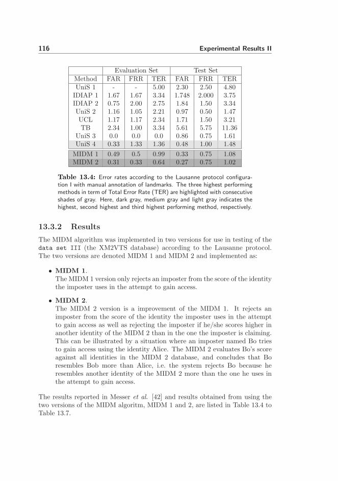
116 Experimental Results II
Evaluation Set Test SetMethod FAR FRR TER FAR FRR TERUniS 1 - - 5.00 2.30 2.50 4.80
IDIAP 1 1.67 1.67 3.34 1.748 2.000 3.75IDIAP 2 0.75 2.00 2.75 1.84 1.50 3.34UniS 2 1.16 1.05 2.21 0.97 0.50 1.47UCL 1.17 1.17 2.34 1.71 1.50 3.21TB 2.34 1.00 3.34 5.61 5.75 11.36
UniS 3 0.0 0.0 0.0 0.86 0.75 1.61UniS 4 0.33 1.33 1.36 0.48 1.00 1.48
MIDM 1 0.49 0.5 0.99 0.33 0.75 1.08MIDM 2 0.31 0.33 0.64 0.27 0.75 1.02
Table 13.4: Error rates according to the Lausanne protocol configura-tion I with manual annotation of landmarks. The three highest performingmethods in term of Total Error Rate (TER) are highlighted with consecutiveshades of gray. Here, dark gray, medium gray and light gray indicates thehighest, second highest and third highest performing method, respectively.
13.3.2 Results
The MIDM algorithm was implemented in two versions for use in testing of thedata set III (the XM2VTS database) according to the Lausanne protocol.The two versions are denoted MIDM 1 and MIDM 2 and implemented as:
• MIDM 1.The MIDM 1 version only rejects an imposter from the score of the identitythe imposter uses in the attempt to gain access.
• MIDM 2.The MIDM 2 version is a improvement of the MIDM 1. It rejects animposter from the score of the identity the imposter uses in the attemptto gain access as well as rejecting the imposter if he/she scores higher inanother identity of the MIDM 2 than in the one the imposter is claiming.This can be illustrated by a situation where an imposter named Bo triesto gain access using the identity Alice. The MIDM 2 evaluates Bo’s scoreagainst all identities in the MIDM 2 database, and concludes that Boresembles Bob more than Alice, i.e. the system rejects Bo because heresembles another identity of the MIDM 2 more than the one he uses inthe attempt to gain access.
The results reported in Messer et al. [42] and results obtained from using thetwo versions of the MIDM algoritm, MIDM 1 and 2, are listed in Table 13.4 toTable 13.7.

13.3 Lausanne Performance Tests 117
Evaluation Set Test SetMethod FAR FRR TER FAR FRR TERIDIAP 1 1.25 1.25 2.5 1.465 2.250 3.715IDIAP 2 0.75 0.75 1.50 1.04 0.25 1.29
TB 1.10 0.50 1.60 3.22 4.50 7.72UniS 4 0.33 0.75 1.08 0.25 0.50 0.75
MIDM 1 0.25 0.25 0.5 0.2 0.75 0.95MIDM 2 0.21 0.25 0.46 0.21 0.5 0.71
Table 13.5: Error rates according to the Lausanne protocol configurationII with manual annotation of landmarks. The three highest performingmethods in term of Total Error Rate (TER) are highlighted with consecutiveshades of gray. Here, dark gray, medium gray and light gray indicates thehighest, second highest and third highest performing method, respectively.
Evaluation Set Test SetMethod FAR FRR TER FAR FRR TERUniS 1 - - 14.0 5.8 7.3 13.1
IDIAP 2 1.21 2.00 3.21 1.95 2.75 4.70UPV 1.33 1.33 2.66 1.23 2.75 3.98
UniS 4 0.82 4.16 4.98 1.36 2.5 3.86
MIDM 1 0.5 0.5 1 0.42 1.25 1.67MIDM 2 0.34 0.5 0.84 0.33 1.25 1.58
Table 13.6: Error rates according to the Lausanne protocol configurationI with automatic annotation of landmarks (Annotations are obtained asdescribed in Section 6.2.3). The three highest performing methods in termof Total Error Rate (TER) are highlighted with consecutive shades of gray.Here, dark gray, medium gray and light gray indicates the highest, secondhighest and third highest performing method, respectively.
Evaluation Set Test SetMethod FAR FRR TER FAR FRR TERIDIAP 2 1.25 1.20 2.45 1.35 0.75 2.10
UPV 1.75 1.75 3.50 1.55 0.75 2.30UniS 4 0.63 2.25 2.88 1.36 2.0 3.36
MIDM 1 0.36 0.67 1.03 0.47 0.75 1.22MIDM 2 0.28 0.5 0.78 0.28 0.75 1.03
Table 13.7: Error rates according to the Lausanne protocol configurationII with automatic annotation of landmarks (Annotations are obtained asdescribed in Section 6.2.3). The three highest performing methods in termof Total Error Rate (TER) are highlighted with consecutive shades of gray.Here, dark gray, medium gray and light gray indicates the highest, secondhighest and third highest performing method, respectively.

118 Experimental Results II
The TER results obtained from the two MIDM methods and the all over bestperforming method presented in the Face Verification Contest, 2003, are takenfrom Table 13.4 to Table 13.7 and shown in a bar plot in Figure 13.5. The allover best performing method presented in the Face Verification Contest, 2003,was UniS 4, presented by the University of Surrey.
Config I manual Config II manual Config I auto Config II auto0
0.5
1
1.5
2
2.5
3
3.5
4
TE
R (
%)
Performance in Total Error Rate
1.48
0.75
3.86
3.36
1.080.95
1.67
1.221.02
0.71
1.58
1.03
UniS 4MIDM 1MIDM 2
Figure 13.5: A bar plot of the TER obtained from the two MIDM meth-ods and from UniS 4.
The results will be discussed in the following section.
13.4 Discussion
From the results obtained in the identification test in Section 13.2.1 it is clearthat the best performance of MIDM is obtained when both the geometrical andthe photometrical information are used. The MIDM algorithm has a higher rateof performance than the Fisherface method (Table 13.1) and has the followingadvantages:
• MIDM is very intuitive. The process used in MIDM to determine whetheror not a person is classified as belonging to a specific model of the MIDMis a one-dimensional problem.
• MIDM is highly flexible and changes in one model do not interfere withthe other models of the MIDM.
• The scalability of MIDM is very high, since the MIDM method can beeasily parallelized to use in a cluster of computers.

13.4 Discussion 119
• No training is needed for the classifier to estimate the FAR. (EstimatingFRR requires training).
In Section 13.2.3 a verification test (a 25-fold cross-validation of data set II)was performed in both a best and a worst case scenario yielding Equal ErrorRates as low as 0.3 and 1.8%, respectively. This is a very satisfying resultobtained from an image data set as large as 700 images.
From the robustness test in Section 13.2.4 a satisfying result was obtained.Changing a persons appearance (i.e. whether or not a person wears spectaclesas well as change in the appearance of the spectacles.) does not result in changeof identity. This result points to the conclusion that face databases should becaptured omitting spectacles.
The performance test in Section 13.3 showed that the MIDM algorithm is su-perior to all the participating methods in the Face Verification Contest in 2003(Figure 13.5).
The MIDM algorithm proposed in Chapter 11 satisfies the demands settled atthe beginning of this thesis, i.e. the objective was to design and develop a robustfacial recognition algorithm constructed in a simple and easy adaptable setup.The results presented in this chapter shows that the MIDM algorithm is a robustand superior face recognition algorithm that is a highly qualified candidate tobe used in a facial recognition application.

120 Experimental Results II

Part IV
Implementation


Chapter 14
Implementation
14.1 Overview
This chapter describes the different implementations developed during this the-sis. These are:
• FaceRec, a Delphi 7 implementation of an automatic facial recognitionprocess using AAM and MIDM.
• A DLL of selected functions of the AAM-API [51].
• A small C++ program used to collect the shape free images and save theseas texture vectors in a Matlab format.
• A Matlab function used to construct the MIDM Model File.
• Various Matlab functions of the described topics in this thesis.
A CD-ROM is enclosed containing all the above mentioned implementations,source code and digital versions of this thesis.
The countless Matlab scripts used to generate the statistical results and the 3Dreconstruction are not included. The Matlab scripts are very comprehensive

124 Implementation
and left out, since they are very machine specific. The specific content of theCD-ROM is listed in Appendix F.
14.2 FaceRec
FaceRec is a Delphi 7 implementation of a real time automatic facial recogni-tion system. FaceRec is implemented for the face recognition task (one to manysearch) and is not expected to encounter unknown persons. FaceRec uses AAMfor face detection and MIDM for face recognition. However, due to time con-straints only texture information is used for face recognition by the MIDM. Thisabolishes the need to implement solution algorithms to Procrustes analysis aswell as the eigenvalue problem in Delphi. A screen shot of FaceRec is displayedin Figure 14.1. A quick user guide is provided in Appendix D.
Figure 14.1: The main window of the FaceRec application, which con-tains an input from a webcam, the shape free image of a captured face, theclass image of the recognized person, a control panel and an AAM/MIDMinformation panel.
A weakness of MIDM is that it is only trained to handle facial images and thealgorithm assumes that the face detection only provides facial images. Thiscauses a problem when MIDM is introduced to non-facial or half facial images.A snapshot of a false recognition due to a non-facial image is displayed in Fig-ure 14.2. It is recommended that the sensitivity of the AAM is kept so highthat only faces are captured. A AAM Model File and a MIDM Model Filebuilt using the IMM Frontal Face Database (data set I) is included on theCD-ROM, however face detection (AAM) will only be optimal when used in thesame lighting condition as the pictures used to build the AAM Model File.
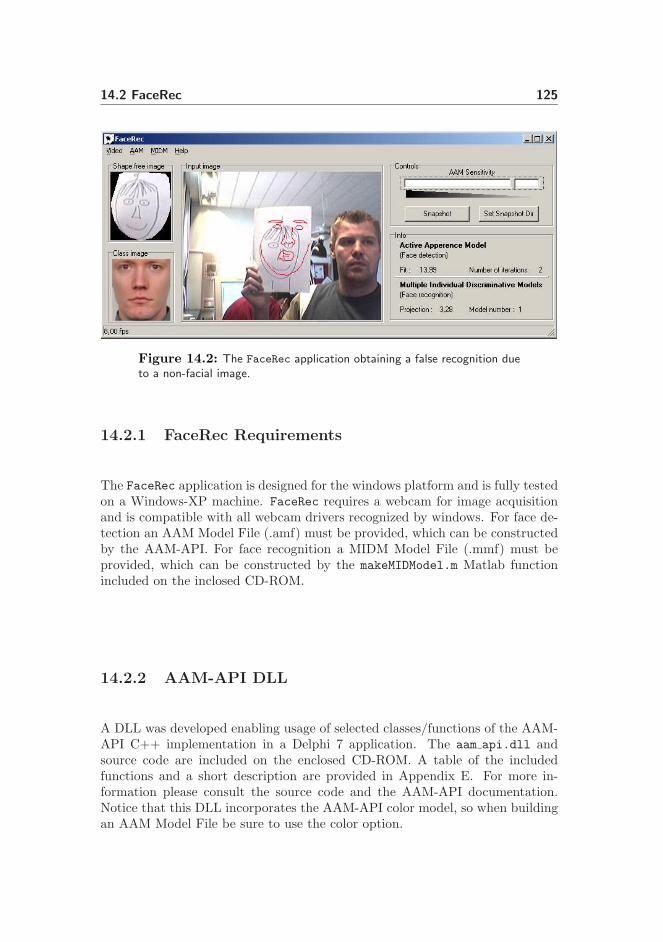
14.2 FaceRec 125
Figure 14.2: The FaceRec application obtaining a false recognition dueto a non-facial image.
14.2.1 FaceRec Requirements
The FaceRec application is designed for the windows platform and is fully testedon a Windows-XP machine. FaceRec requires a webcam for image acquisitionand is compatible with all webcam drivers recognized by windows. For face de-tection an AAM Model File (.amf) must be provided, which can be constructedby the AAM-API. For face recognition a MIDM Model File (.mmf) must beprovided, which can be constructed by the makeMIDModel.m Matlab functionincluded on the inclosed CD-ROM.
14.2.2 AAM-API DLL
A DLL was developed enabling usage of selected classes/functions of the AAM-API C++ implementation in a Delphi 7 application. The aam api.dll andsource code are included on the enclosed CD-ROM. A table of the includedfunctions and a short description are provided in Appendix E. For more in-formation please consult the source code and the AAM-API documentation.Notice that this DLL incorporates the AAM-API color model, so when buildingan AAM Model File be sure to use the color option.

126 Implementation
14.2.3 Make MIDM Model File
The Matlab function makeMIDModel.m is used to construct the MIDM ModelFile used by FaceRec. The function only implements the MIDM algorithm fortexture information. In order to retrieve texture vectors from free shape imagesa small C++ application is developed. For more information please consult thesource code or type “help makeMIDModel” in Matlab.
14.2.3.1 Get Texture Vectors
The getTextureVectors.exe C++ application opens an AAM Model File andsaves the texture vectors of the free shape images obtained from all imagesresiding in the same folder as the AAM Model File, in a Matlab format.
14.3 Matlab Functions
The following Matlab functions were developed during this thesis and are in-cluded on the enclosed CD-ROM for possible future use.
• flda.m
Fisher linear discriminant analysis, described in Section 9.2.
• histEqImage.m
Histogram equalization of an image, described in Section 8.1.1.
• kNearNeighbor.m
k nearest neighbor algorithm.
• lightCompensationModels.m
Removal of specific illumination conditions based on illumination compen-sation models, as described in Section 8.1.2.
• lpp.m
Locality preserving projections, described in Section 9.3.
• pca minMem.m
Principal component analysis, using the method described in Section 9.1.2,to achieve a speedup and reduction in memory usage.

14.4 Pitfalls 127
• pca numberOfEigenvectors.m
This function calculates the number of eigenvectors needed to capture acertain percentage of the image variance, as described in Eq. 7.2.
pca minMem.m and pca numberOfEigenvectors.m are used by makeMIDModel.m.The readasf.m Matlab function distributed with the AAM-API for reading asf
files is also included in the inclosed CD-ROM. The results in Chapter 10 forthe KFDA method was obtained by the Generalized Discriminant Analysis GDAMatlab package provided by Baudat et al. [3].
14.4 Pitfalls
Two tricky issues of implementation are highlighted in the following, passingarrays and the Matlab eig function.
14.4.1 Passing Arrays
When passing an array from Delphi to C++ the array is received by C++ asa array pointer and the length of the array. An example is provided in thefollowing by the function in the aam api.dll for retrieving the center of gravityof a shape:
Call from Delphi:
procedure shapeCOG_dll(shape:CAAMShapeHandle;
var shapeCOG : array of double); stdcall;
Function in the DLL (C++):
void __declspec(dllexport) shapeCOG(CAAMShapeHandle shape,
double *shapeCOG, int arraylength);
14.4.2 The Matlab Eig Function
When solving the eigenvalue problem in Matlab by using the function eig onehas to consider that Matlab release 14 (used in this thesis) does not guarantee

128 Implementation
that eigenvalues and eigenvectors are sorted in ascending order (which was thecase for Matlab release 13). To overcome this the following code snippet can beused:
[eigV eigD]=eig(covarianceMatrix);
%Most important eigenvalue at buttom (right) Needs
%to be sorted, there is a "bug" (change) in Matlab R 14 eig.
[sorted I] = sort(sum(eigD));
eigV = eigV(:,I);
eigD = diag(sorted);

Part V
Discussion


Chapter 15
Future Work
The following sections describe interesting areas which could improve the facialrecognition of the MIDM algorithm.
15.1 Light Normalization
One way to improve the robustness and flexibility of the MIDM algorithm isto improve light normalization/correlation in the preprocess step. Looking intomethods that can remove specific light sources leaving the facial image in adiffuse lighting is very interesting and can lead to the following improvements:
• Successful implementation of the MIDM algorithm in environments withlarge variation in lighting conditions.
• An increase in performance of the MIDM algorithm, since it does not needto be trained to be capable of handling multi-lighting conditions.
• The enrollment of new persons in the MIDM scheme would be a muchsimpler and more robust process.
132 Future Work
15.2 Face Detection
From an implementation point of view proper face detection is very importantin a face recognition process. The performance of a face recognition scheme canbe notably improved by minimizing the false detection of faces. As describedin Chapter 14 the MIDM algorithm shows a weakness when it is presented toa non-facial image, since it is not trained to handle the variation of non-facialimages, resulting in a possible misclassification. In addition, the face detectionalgorithm (AAM) used in the implementation described in Chapter 14 is verysensitive to specific lighting condition, which causes a problem. Decreasing theAAM sensitivity towards specific lighting conditions would be an area of greatinterest.
15.3 3D Facial Reconstruction
As described in Chapter 12 facial reconstruction in 3D from 2D images is a veryinteresting area. The end goal is extraction of more discriminative 3D informa-tion from which a better face recognition performance could be obtained com-pared to that from 2D images. Reconstruction and recognition of not frontal faceimages through 3D images are of great interest as well. The interest in this areais not limited to facial recognition, since reconstruction of a three-dimensionalshape without use of 3D scanners would be useable in many applications as well.

Chapter 16
Discussion
16.1 Summary of Main Contributions
The following four sections describe the main contributions of this thesis tofacial recognition.
16.1.1 IMM Frontal Face Database
As a part of this thesis the IMM Frontal Face Database was constructed for usein the initial testing of feature extraction methods. The database consists of 120images of 12 persons and is described in detail in Appendix A. The database onlycontains small variation (in term of facial poses, illumination conditions, etc.),which makes it an ideal database when working in a low-dimensional featurespace, e.g. in dimension one to five. However, to obtain reliable performancetests one need to use other databases with more variation.

134 Discussion
16.1.2 The MIDM Algorithm
A central part in this thesis is the development of the Multiple Individual Dis-criminative Models (MIDM) algorithm, as described in Chapter 11. MIDM isa feature extraction and identity matching algorithm, which has been provenvery robust and adaptive (see Chapter 13).
16.1.3 A Delphi Implementation
A Delphi implementation of an automated face recognition scheme was con-structed as described in Chapter 14. The implementation includes a DLL, in-corporating a C++ implementation of Active Appearance Models (AAM-API[51]). The implementation is designed for the windows platform and requires awebcam for image acquisition.
16.1.4 Matlab Functions
The following Matlab functions were constructed and used in this thesis:
• flda.m
Fisher linear discriminant analysis, described in Section 9.2.
• histEqImage.m
Histogram equalization of an image, described in Section 8.1.1.
• kNearNeighbor.m
k nearest neighbor algorithm.
• lightCompensationModels.m
Removal of specific illumination conditions based on illumination compen-sation models, as described in Section 8.1.2.
• lpp.m
Locality preserving projections, described in Section 9.3.
• pca minMem.m
Principal component analysis, using the method described in Section 9.1.2,to achieve a speedup and reduction in memory usage.

16.2 Conclusion 135
16.2 Conclusion
The increase in complexity in consumer goods such as automobiles and homeappliances provides for a new market for technologies such as face recognition.Additionally, the recent events in the world has spurred a public demand forsecurity and safety in public places; demands that could be partially met bydeployment of these technologies.
The four objectives of this thesis were: To discuss and summarize the processof facial recognition, to look at currently available facial recognition techniques,to design and develop a robust facial recognition algorithm and finally an im-plementation of this new algorithm.
In Chapter 2 to Chapter 10 this thesis presents a comprehensive overview of thearea of facial recognition, satisfying the two first objectives. The third objectiveof this thesis is satisfied by the work presented in Chapter 11 to Chapter 13by the design and development of MIDM, a new feature extraction and identitymatching algorithm. By tests in the mentioned chapters MIDM has been provensuperior to all participating methods in the Face Verification Contest at TheAudio Video Biometric Person Authentication Conference in 2003. MIDM is toparticipate in the Face Verification Contest at the International Conference onBiometrics in Hong Kong in January, 2006.
The last objective is satisfied by the work presented in Chapter 14. The im-plementation of the MIDM algorithm does not require any special hardwarebesides a webcam for collection of input images.
Though MIDM has been developed to be used in the process of facial recognitionthe algorithm can easily be adapted to recognize other objects. This makesMIDM a useful algorithm in more than one sense.
With the completion of this thesis, an important step in addressing the qualityand reliability of face recognition schemes has been completed.

136 Discussion

List of Figures
1.1 Comparison of machine readable travel documents (MRTD) com-patibility with six biometric techniques. . . . . . . . . . . . . . . 2
1.2 “The Wife and the Mother-in-Law” by Edwin G. Boring. . . . . 3
3.1 Relation of False Acceptance Rate (FAR), False Rejection Rate(FRR) with the distribution of clients, imposters in a verificationscheme. . . . . . . . . . . . . . . . . . . . . . . . . . . . . . . . . 15
3.2 The Correct Identification Rates (CIR) plotted as a function ofgallery size. . . . . . . . . . . . . . . . . . . . . . . . . . . . . . . 18
3.3 The average Correct Identification Rates (CIR) of the three high-est performing systems in the Face Recognition Vendor Test 2002from a age perspective. . . . . . . . . . . . . . . . . . . . . . . . . 18
3.4 The average Correct Identification Rates (CIR) of the three high-est performing systems in the Face Recognition Vendor Test 2002from a time perspective. . . . . . . . . . . . . . . . . . . . . . . . 19
4.1 The four general steps in facial recognition. . . . . . . . . . . . . 22
5.1 Small interpersonal variations illustrated by identical twins. . . . 26

138 LIST OF FIGURES
5.2 A sample of 33 facial images produced from one original image. . 28
5.3 Results of the exploration of facial submanifolds. . . . . . . . . . 29
5.4 An illustration of the problem of not being capable of satisfactoryapproximating the manifold when only having a small number ofsamples. . . . . . . . . . . . . . . . . . . . . . . . . . . . . . . . . 31
6.1 An example of ten images of one person from the IMM FrontalFace Database. . . . . . . . . . . . . . . . . . . . . . . . . . . . . 37
6.2 The 73-landmark annotation scheme used on the IMM FrontalFace Database. . . . . . . . . . . . . . . . . . . . . . . . . . . . . 38
6.3 Examples of 14 images of one female and one male obtained fromthe AR database. . . . . . . . . . . . . . . . . . . . . . . . . . . . 39
6.4 The 22-landmark annotation scheme used on the AR database. . 40
6.5 Examples of 8 images of one female and one male obtained fromthe XM2VTS database. . . . . . . . . . . . . . . . . . . . . . . . 42
6.6 The 64-landmark annotation scheme used on the XM2VTS data-base. . . . . . . . . . . . . . . . . . . . . . . . . . . . . . . . . . . 43
6.7 Five samples from 3D Face Database constructed in [49]. . . . . . 44
7.1 Illustration of the subsampling of an image in a pyramid fashion.Which enables the capture of different size of faces. . . . . . . . . 50
7.2 Example of 10 Eigenfaces. . . . . . . . . . . . . . . . . . . . . . . 51
7.3 Diagram of the neural network developed by Rowley et al. [47]. . 53
7.4 Diagram displaying an improved version of the neural network inFigure 7.3. . . . . . . . . . . . . . . . . . . . . . . . . . . . . . . . 54
7.5 Example of full Procrustes analysis. . . . . . . . . . . . . . . . . 55
7.6 Face detection (approximations) obtained by AAM, when themodel is initialized close to the face. . . . . . . . . . . . . . . . . 57

LIST OF FIGURES 139
8.1 Examples of histogram equalization used upon two images to ob-tain standardized images with maximum entropy. . . . . . . . . . 60
8.2 Removal of specific illumination conditions from facial images. . 62
8.3 A close-up of the faces reconstructed in Figure 8.2. . . . . . . . . 62
8.4 Illumination compensation maps used for removal of specific illu-mination conditions. . . . . . . . . . . . . . . . . . . . . . . . . . 63
9.1 An example of PCA in two dimensions. . . . . . . . . . . . . . . 66
9.2 An example of FLDA in two dimensions. . . . . . . . . . . . . . . 69
10.1 The PCA scatter plot matrix of the combined features from data
set I. . . . . . . . . . . . . . . . . . . . . . . . . . . . . . . . . . 81
10.2 The LPP scatter plot matrix of the combined features from data
set I. . . . . . . . . . . . . . . . . . . . . . . . . . . . . . . . . . 82
10.3 The FLDA scatter plot matrix of the combined features fromdata set I. . . . . . . . . . . . . . . . . . . . . . . . . . . . . . . 83
10.4 The KFDA scatter plot matrix of the combined features fromdata set I. . . . . . . . . . . . . . . . . . . . . . . . . . . . . . . 84
10.5 False identification rates obtained from the 50/50 test, wheredata set I is divided into two equal sized sets, a training setand a test set. . . . . . . . . . . . . . . . . . . . . . . . . . . . . . 85
10.6 The false identification rates obtained from the ten-fold cross-validation test. . . . . . . . . . . . . . . . . . . . . . . . . . . . . 86
11.1 Overview of the MIDM algorithm. . . . . . . . . . . . . . . . . . 93
11.2 Example of a Delaunay triangulation of the landmark scheme indata set II. . . . . . . . . . . . . . . . . . . . . . . . . . . . . . 94
12.1 Process of projecting 3D landmarks into a 2D image, which isused to calculate a fit of the 3D shape. . . . . . . . . . . . . . . . 100

140 LIST OF FIGURES
12.2 Example of retrieved depth information from a 2D frontal faceimage. . . . . . . . . . . . . . . . . . . . . . . . . . . . . . . . . . 101
12.3 Example of retrieved depth information from a 2D frontal faceimage and a 2D profile face image. . . . . . . . . . . . . . . . . . 102
13.1 Importance of geometrical information. . . . . . . . . . . . . . . . 108
13.2 The 10%, 15% and 25% pixels weights of highest value most im-portant for discrimination between the test persons of data set
II. . . . . . . . . . . . . . . . . . . . . . . . . . . . . . . . . . . . 109
13.3 False Acceptance Rate and False Rejections Rate graphs and Re-ceiver Operating Characteristic (ROC) curve obtained by the 25-fold cross-validation for the best and worst case scenario, respec-tively. . . . . . . . . . . . . . . . . . . . . . . . . . . . . . . . . . 111
13.4 Effect of change in a persons appearance, illustrated by superim-posing spectacles onto a person from data set II not wearingspectacles. . . . . . . . . . . . . . . . . . . . . . . . . . . . . . . . 114
13.5 A bar plot of the TER obtained from the two MIDM methodsand from UniS 4. . . . . . . . . . . . . . . . . . . . . . . . . . . . 118
14.1 The main window of the FaceRec application. . . . . . . . . . . . 124
14.2 The FaceRec application obtaining a false recognition due to anon-facial image. . . . . . . . . . . . . . . . . . . . . . . . . . . . 125
D.1 The main window of the FaceRec application. . . . . . . . . . . . 174
D.2 The video driver list popup box. . . . . . . . . . . . . . . . . . . 174
D.3 The specific “Video Source” panel included in the drivers of thePhilips PCVC690K webcam. . . . . . . . . . . . . . . . . . . . . 175
D.4 The FaceRec application capturing a face and recognizing it asmodel (person) number 8. . . . . . . . . . . . . . . . . . . . . . . 176
F.1 The contents of the enclosed CD-ROM. . . . . . . . . . . . . . . 182

List of Tables
3.1 Participants in the Face Recognition Vendor Test 2002. . . . . . 16
3.2 The characteristics of the highest performing systems in the FaceRecognition Vendor Test 2002. . . . . . . . . . . . . . . . . . . . 17
7.1 Categorization of methods for face detection within a single image. 49
9.1 Dimensionality reduction methods. . . . . . . . . . . . . . . . . . 65
13.1 Correct identification rates. . . . . . . . . . . . . . . . . . . . . . 108
13.2 Partitioning of data set III according to the Lausanne protocolconfiguration I. . . . . . . . . . . . . . . . . . . . . . . . . . . . . 113
13.3 Partitioning of data set III according to the Lausanne protocolconfiguration II. . . . . . . . . . . . . . . . . . . . . . . . . . . . . 115
13.4 Error rates according to the Lausanne protocol configuration Iwith manual annotation of landmarks. . . . . . . . . . . . . . . . 116
13.5 Error rates according to the Lausanne protocol configuration IIwith manual annotation of landmarks. . . . . . . . . . . . . . . . 117

142 LIST OF TABLES
13.6 Error rates according to the Lausanne protocol configuration Iwith automatic annotation of landmarks. . . . . . . . . . . . . . 117
13.7 Error rates according to the Lausanne protocol configuration IIwith automatic annotation of landmarks. . . . . . . . . . . . . . 117
E.1 Function list over the aam api.dll. . . . . . . . . . . . . . . . . . 178
E.2 Function list over the aam api.dll continued. . . . . . . . . . . . 179

Appendix A
The IMM Frontal Face
Database

144 Appendix A

The IMM Frontal Face Database 145
The IMM Frontal Fa e DatabaseAn Annotated Dataset of 120 Frontal Fa e ImagesJens Fagertun and Mikkel B. StegmannInformati s and Mathemati al Modelling, Te hni al University of DenmarkRi hard Petersens Plads, Building 321, DK-2800 Kgs. Lyngby, Denmark29. August 2005Abstra tThis note des ribes a data set onsisting of 120 annotated mono ular images of 12 di�erentfrontal human fa es. Points of orresponden e are pla ed on ea h image so the data set an bereadily used for building statisti al models of shape. Format spe i� ations and terms of use arealso given in this note.Keywords: Annotated image data set, frontal fa e images, statisti al models of shape.1 Data Set Des riptionThis database onsists of 12 people (all male). A total of 10 frontal fa e photos has been re ordedof ea h person. The data set is ontaining di�erent fa ial poses aptured over a short period oftime, with a minimum of varian e in lighting, amera position, et .All photos are annotated with landmarks de�ning the eyebrows, eyes, nose, mouth and jaw,see Figure 1. The annotation of ea h photo is stored in the ASF format, des ribed in AppendixA.2 Spe i� ations2.1 General Spe i� ations2.1.1 Spe i� ations of Test PersonsAll test persons are males, not wearing glasses, hats or other a essories.2.1.2 Spe i� ations of Fa ial ExpressionsTable 1 lists the fa ial expressions aptured in this data set.Fa ial expressions Des riptionNo expression The normal fa ial poseRelaxed happy Smiling vaguely (lips losed)Relaxed thinking The fa ial expression is a little tense (try to multiply 57*9 ; )Table 1: Spe i� ations of fa ial expressions.1

146 Appendix A
Figure 1: The 73 landmarks annotation de�ning the fa ial features; eye-brows, eyes, nose, mouth and jaw.2

The IMM Frontal Face Database 1472.1.3 Image Format and NamingThe images are in JPEG format and named XX_YY.jpg where XX is the person id and YY the photonumber. Table 2 shows the orresponden e between the photo number and the fa ial expression.Photo number Fa ial expression01 to 06 No expression07 to 08 Relaxed happy09 to 10 Relaxed thinkingTable 2: Photo number spe i� ation.2.1.4 Annotation Spe i� ationsAll photos were annotated with 73 landmarks. Table 3 spe i�es the orresponden e betweenannotation landmarks and fa ial features. For the pre ise landmark pla ements see Figure 1.Fa ial Features Annotation landmarksRight eyebrow 1 - 8Left eyebrow 9 - 16Right eye 17 - 24Left eye 25 - 32Right eyes pupil 33Left eyes pupil 34Nose 35 - 46Mouth 47 - 62Jaw 63 - 73Table 3: The 73 landmarks annotation de�ning the fa ial features; eyebrows,eyes, nose, mouth and jaw.2.2 Studio Spe i� ationsFigure 2 displays the studio setup.2.2.1 Spe i� ation of Ba kdropIn this data set a white proje tor s reen is used as ba kdrop, whi h is a uniform nonre�e tingsurfa e, distinguishable from the test persons skin, hair and lothes. The amera lens has to beparallel to the ba kground.2.2.2 Spe i� ations of Camera and Person Pla ementThe person was sitting down on an o� e hair and �lmed with a straight ba k. The amera waspla ed in the same height as the test person eyes. The fa e of the test person was parallel tothe ba kground and the amera lens. An example of a full size image is shown in Figure 3. The amera aptures additional spa e above and below the head of the test person in order to insure,that all test persons an be re orded without altering the studio setup.2.2.3 Spe i� ations of LightThe di�use light is oming solely from two spot lights. The light was boun ed o� using whiteumbrellas. In the studio there was no interferen e from sun light, room light et .3
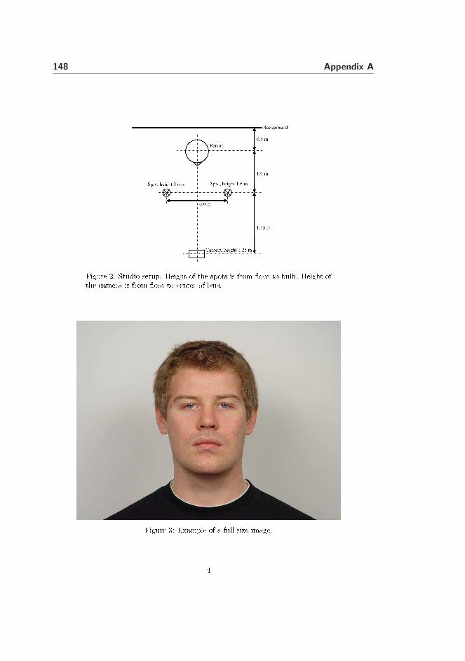
148 Appendix A
Figure 2: Studio setup: Height of the spots is from �oor to bulb. Height ofthe amera is from �oor to enter of lens.
Figure 3: Example of a full size image.4

The IMM Frontal Face Database 1492.3 Te hni al Spe i� ations2.3.1 Camera Spe i� ationsName Sony - Cyber-shotImage size 5.0 megapixelsModel no DSC-F7172.3.2 Image Spe i� ationsFo al length 48 mm1Compression Fine/Normal (jpg)2Iso speed 200Aperture F/2.4Shutter speed 1/100 sImage size 2560 × 1920 pixelsExposure Compensation + 0.7 EVWhite balan e Custom32.3.3 Spot Light Spe i� ationsSpot Light: Manufa turer HedlerName Videolux 300Bulb: Manufa turer OsramType HalogenName Photo Opti LampNo 64515Watt 300 w3 The Work Pro ess Proto ol of One Test Person1. The amera position is pla ed a ordingly to the spe i� ations above (approx 1.25 m from�oor to lens and same level as the eyes of the test person).2. The test person is explained the meaning of the pose to be re orded, in terms of the fa ialexpression.3. The test person is distra ted for one se ond to "reset" fa ial features (ex. rolls with thehead), and assumes the wanted pose, the photo is re orded. (Make sure the test personspit h, roll and yaw is not to riti al ompared to the amera lens. Nostrils should be justvisible).4. Item 3. is repeated until all the photos of this pose are re orded.5. Item 2. is repeated for all the wanted poses.6. Re ord the test persons age.1Equivalent to 190 mm with a 35 mm FOV.2The average �le size was 1.9MB.3The white balan e on the amera was alibrated to the ba kdrop with the spotlights.5

150 Appendix A4 Things to Improve• Green ba kground (not shiny).• More di�use lighting (the lighting an be pla ed further away from the test person).• A real photo hair (not an o� e hair).• Fixed fo al length (a amera where you an see the urrent exa t fo al length).• Stri t rules for test persons pit h, roll and yaw.5 Terms of UseThe data set an be freely used for edu ation and resear h. The only requirement is that areferen e to this note is given.
6

The IMM Frontal Face Database 151A ASF � AAM Shape Format Spe i� ationAn ASF �le is stru tured as a set of lines separated by a CR hara ter. Anywhere in the �le, omments an be added by starting a line with the '#' hara ter. Comment lines and empty linesare dis arded prior to parsing. The layout of an ASF �le is as follows:• Line 1 ontains the total number of points, n, in the shape.• Line 2 to n+1 ontains the point information (one line per point) su h as the point lo ation,type, onne tivity et ., see below. Hen e, qui k and simple a ess is preferred over data ompa tness.• Line n+2 ontains the host image, i.e. the �lename of the image where the annotation isde�ned.The formal point de�nition is:point := <path#> <type> <x-pos> <y-pos> <point#> < onne ts from> < onne ts to>
<path#> The path that the point belongs to. Points from di�erent paths must not be inter hanged (in theline order).<type> A bitmapped �eld that de�nes the type of point:
• Bit 1: Outer edge point/Inside point• Bit 2: Original annotated point/Arti� ial point• Bit 3: Closed path point/Open path point• Bit 4: Non-hole/Hole pointRemaining bits should be set to zero. An inside arti� ial point whi h is a part of an losed hole, has thusthe type: (1�1) + (1�2) + (1�4) = 1 + 2 + 4 = 7.
<x-pos> The relative x-position of the point. Obtained by dividing image oordinates in the range [0;image width-1℄by the image width (due to strange histori reasons...). Thus, pixel x = 47 (the 48th pixel) in a 256 pixelwide image has the relative position 47/256 = 0.18359375.<y-pos> The relative y-position of the point. Obtained by dividing image oordinates in the range [0;image height-1℄by the image height (due to strange histori reasons...). Thus, pixel y = 47 (the 48th pixel) in a 256pixel tall image has the relative position 47/256 = 0.18359375.<point#> The point number. First point is zero. This is merely a servi e to the human reader sin e theline at where the point o urs impli itly gives the real point number.< onne ts from> The previous point on this path. If none < onne ts from> == <point#> an be used.< onne ts to> The next point on this path. If none < onne ts to> == <point#> an be used.Further, the following format rules apply:
• Fields in a point spe i� ation are separated by spa es or tabs.• Path points are assumed to be de�ned lo kwise. That is; the outside normal is de�ned tobe on left of the point in the lo kwise dire tion. Holes are thus de�ned ounter- lo kwise.• Points are de�ned in the fourth quadrant. Hen e, the upper left orner pixel is (0,0).• Isolated points are signaled using < onne ts from> == < onne ts to> == <point#>.• A shape must have at least one outer edge. If the outer edge is open, the onvex hull shoulddetermine the interior of the shape. 7

152 Appendix AExample ASF �le<BOF>######################################################################### AAM Shape File - written: Monday May 08 - 2000 [15:22℄########################################################################## number of model points#83## model points## format: <path#> <type> <x rel.> <y rel.> <point#> < onne ts from> < onne ts to>#0 0 0.07690192 0.44500541 0 82 10 0 0.09916206 0.42914406 1 0 20 0 0.12925033 0.39573063 2 1 3...0 0 0.07579006 0.52910086 80 79 810 0 0.06128729 0.49762829 81 80 820 0 0.05858913 0.46610570 82 81 0## host image#F1011flb.bmp<EOF>
8

Appendix B
A face recognition algorithm
based on MIDM

154 Appendix B

A face recognition algorithm based on MIDM 155
PROCEEDINGS OF THE 14TH DANISH CONFERENCE ON PATTERN RECOGNITION AND IMAGE ANALYSIS 2005 1
A face recognition algorithm based on multipleindividual discriminative models
Jens Fagertun, David Delgado Gomez, Bjarne K. Ersbøll, Rasmus Larsen
Abstract— In this paper, a novel algorithm for facial recogni-tion is proposed. The technique combines the color texture andgeometrical configuration provided by face images. Landmarksand pixel intensities are used by Principal Component Analysisand Fisher Linear Discriminant Analysis to associate a onedimensional projection to each person belonging to a referencedata set. Each of these projections discriminates the associatedperson with respect to all other people in the data set. Theseprojections combined with a proposed classification algorithm areable to statistically deciding if a new facial image corresponds to aperson in the database. Each projection is also able to visualizingthe most discriminative facial features of the person associated tothe projection. The performance of the proposed method is testedin two experiments. Results point out the proposed technique asan accurate and robust tool for facial identification and unknowndetection.
Index Terms— Face recognition, Principal Component Anal-ysis, Fisher Linear Discriminant Analysis, Biometrics, Multi-Subspace Method.
I. I NTRODUCTION
Regrettable events which happened during the last years(New York, Madrid) have revealed flaws in the existingsecurity systems. The vulnerability of most of the current se-curity and personal identification system is frequently shown.Falsification of identity cards or intrusion into physical andvirtual areas by cracking alphanumerical passwords appearfrequently in the media. These facts have triggered a realnecessity for reliable, user-friendly and widely acceptablecontrol mechanisms for person identification and verification.
Biometrics, which bases the person authentication on the in-trinsic aspects of a human being, appears as a viable alternativeto more traditional approaches (such as PIN codes or pass-words). Among the oldest biometrics techniques, fingerprintrecognition can be found. It is known that this technique wasused in China around 700 AD to officially certify contracts.Afterwards, in Europe, it was used as person identificationin the middle of the19th century. A more recent biometrictechnique used for people identification is iris recognition [8].It has been calculated that the chance of finding two randomlyformed identical irises is one in1078 (The population of theearth is below1010) [7]. This technique has started to beused as and alternative to passport in some airports in UnitedKingdom, Canada and Netherlands. It is also used as employeecontrol access to restricted areas in Canadian airports andin the New York JFK airport. The inconvenient of thesetechniques is the necessity of interaction with the individualwho wants to be identified or authenticated. This fact hascaused that face recognition, a non-intrusive technique, has
increasedly received the interest from the scientific communityin recent years.
The first developed techniques that aimed at identifyingpeople from facial images were based on geometrical infor-mation. Relative distances between key points, such as mouthcorners or eyes, were calculated and used to characterizefaces [17]. Therefore, most of the developed techniques duringthe first stages of facial recognition focused on the automaticdetection of individual facial features. However, facial featuredetection and measurements techniques developed to date arenot reliable enough for the geometric feature based recog-nition, and such geometric properties alone are inadequatefor face recognition because rich information contained inthefacial texture or appearance is discarded [6], [13]. This factproduced that gradually most of the geometrical approacheswere abandoned for color based techniques, which providedbetter results. These methods aligned the different faces toobtain a correspondence between pixels intensities. A nearestneighbor classifier used these aligned values to classify thedifferent faces. This coarse method was notably enhancedwith the appearance of the Eigenfaces technique [15]. Insteadof directly comparing the pixel intensities of the differentface images, the dimension of these input intensities werefirst reduced by a principal component analysis (PCA). Thistechnique settled the basis of many of the current image basedfacial recognition schemes. Among these current techniques,Fisherfaces can be found. This technique, widely used andreferred [2], [4], combines the Eigenfaces with Fisher lineardiscriminant analysis (FLDA) to obtain a better separationof the individuals. In Fisherfaces, the dimension of the inputintensity vectors is reduced by PCA and then FLDA is appliedto obtain a good separation of the different persons.
After Fisherfaces, many related techniques have been pro-posed. These new techniques aim at providing a projectionthat attain a good person discrimination and also are robustatdifferences in illumination or image pose. Kernel Fisherfaces[16], Laplacianfaces [10] or discriminative common vectors[3] can be found among these new approaches. Typically, thesetechniques have been tested assuming that the image to beclassified corresponds to one of the people in the database. Inthese approaches, the image is usually classified to the personwith the smallest Euclidean distance.
However, some inconveniences appear when the person tobe analyzed may not belong to the data set. In this case, acriterium to decide if the person belongs to the data set hasto be chosen. E.g. only people with an euclidian distance lessthan a given threshold are considered as belonging to the dataset. However, this threshold has not to be necessarily the same
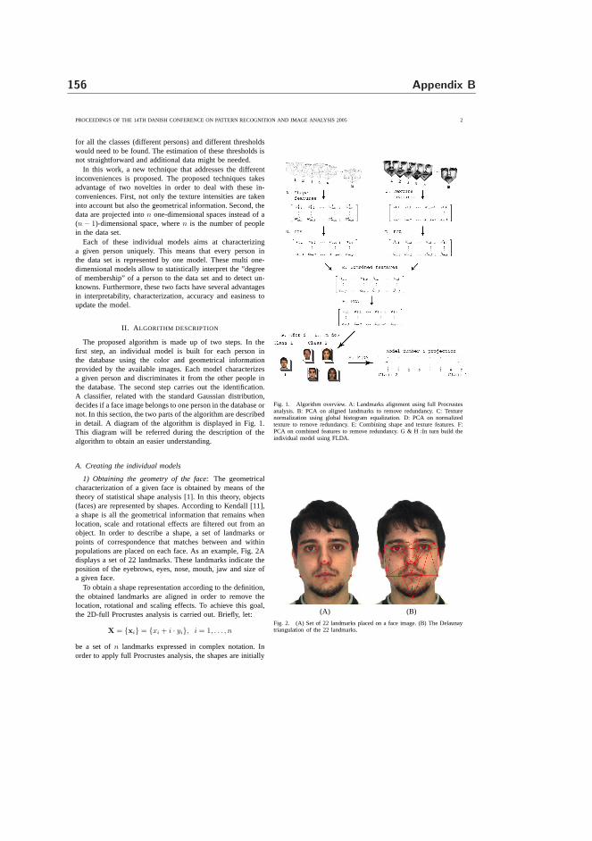
156 Appendix B
PROCEEDINGS OF THE 14TH DANISH CONFERENCE ON PATTERN RECOGNITION AND IMAGE ANALYSIS 2005 2
for all the classes (different persons) and different thresholdswould need to be found. The estimation of these thresholds isnot straightforward and additional data might be needed.
In this work, a new technique that addresses the differentinconveniences is proposed. The proposed techniques takesadvantage of two novelties in order to deal with these in-conveniences. First, not only the texture intensities are takeninto account but also the geometrical information. Second,thedata are projected inton one-dimensional spaces instead of a(n − 1)-dimensional space, wheren is the number of peoplein the data set.
Each of these individual models aims at characterizinga given person uniquely. This means that every person inthe data set is represented by one model. These multi one-dimensional models allow to statistically interpret the ”degreeof membership” of a person to the data set and to detect un-knowns. Furthermore, these two facts have several advantagesin interpretability, characterization, accuracy and easiness toupdate the model.
II. A LGORITHM DESCRIPTION
The proposed algorithm is made up of two steps. In thefirst step, an individual model is built for each person inthe database using the color and geometrical informationprovided by the available images. Each model characterizesa given person and discriminates it from the other people inthe database. The second step carries out the identification.A classifier, related with the standard Gaussian distribution,decides if a face image belongs to one person in the database ornot. In this section, the two parts of the algorithm are describedin detail. A diagram of the algorithm is displayed in Fig. 1.This diagram will be referred during the description of thealgorithm to obtain an easier understanding.
A. Creating the individual models
1) Obtaining the geometry of the face:The geometricalcharacterization of a given face is obtained by means of thetheory of statistical shape analysis [1]. In this theory, objects(faces) are represented by shapes. According to Kendall [11],a shape is all the geometrical information that remains whenlocation, scale and rotational effects are filtered out fromanobject. In order to describe a shape, a set of landmarks orpoints of correspondence that matches between and withinpopulations are placed on each face. As an example, Fig. 2Adisplays a set of 22 landmarks. These landmarks indicate theposition of the eyebrows, eyes, nose, mouth, jaw and size ofa given face.
To obtain a shape representation according to the definition,the obtained landmarks are aligned in order to remove thelocation, rotational and scaling effects. To achieve this goal,the 2D-full Procrustes analysis is carried out. Briefly, let:
X = {xi} = {xi + i · yi}, i = 1, . . . , n
be a set ofn landmarks expressed in complex notation. Inorder to apply full Procrustes analysis, the shapes are initially
Fig. 1. Algorithm overview. A: Landmarks alignment using full Procrustesanalysis. B: PCA on aligned landmarks to remove redundancy.C: Texturenormalization using global histogram equalization. D: PCAon normalizedtexture to remove redundancy. E: Combining shape and texture features. F:PCA on combined features to remove redundancy. G & H :In turn build theindividual model using FLDA.
(A) (B)
Fig. 2. (A) Set of 22 landmarks placed on a face image. (B) The Delaunaytriangulation of the 22 landmarks.

A face recognition algorithm based on MIDM 157
PROCEEDINGS OF THE 14TH DANISH CONFERENCE ON PATTERN RECOGNITION AND IMAGE ANALYSIS 2005 3
(A) (B)
Fig. 3. (A) Superimposition of the sets of 22 landmarks obtained over 49different face images. (B) Alignment of the landmarks.
centered. To center the different shapes, the mean of the shape,x, is subtracted from each landmark:
wi = xi − x, i = 1, . . . , n
.The full Procrustes mean shape [12],µ, is found as the
eigenvector corresponding to the largest eigenvalue of thecomplex sum of squares and products matrix
n∑
i=1
wiw∗
i /(w∗
i wi)
where w∗
i denotes the transpose of the complex conjugateof wi. Using this Procrustes mean shape, the full Procrustescoordinates ofw1, . . . ,wn (Fig. 1) A) are obtained by
wPi = w
∗
i µwi/(w∗
i wi) i = 1, . . . , n
Fig. 3A displays the superimposition of the set of 22landmarks described in Fig. 2, obtained on 49 different faceimages. The result obtained after applying the full Procustresalignment on theses landmarks can be observed in Fig. 3B.In order to remove redundancy in the data, a Principal Com-ponent Analysis is applied to the aligned landmarks (Fig. 1B).
2) Texture formulation: To form a complete model ofthe face appearance, the algorithm also captures the textureinformation provided by the pixels. In order to collect thistexture representation, the Delaunay triangulation of everyshape is obtained. The Delanuay triangulation connects thealigned landmark set of each image by a mesh of triangles,so no triangle has any of the other points of the set insideits circumcircle. The Delaunay triangulation obtained foreachimage is warped onto the Delaunay triangulation of the meanshape. The Delanuay triangulation of the 22 landmarks isdisplayed in Fig. 2B.
Formally, let I be a given image andM the mean shapepreviously obtained. Letu1 = [x1, y1],u2 = [x2, y2] andu3 =[x3, y3] denote the vertices of a triangleT in I, and letv1,v2
andv3 be the associated vertices of the corresponding trianglein M . Given any internal pointu = [x, y] in the triangleT ,the corresponding point in the associated triangle in the meanshape can be written asv = αv1 + βv2 + γv3 where:
α = 1 − (β + γ)
β =yx3 − x1y − x3y1 − y3x + x1y3 + xy1
−x2y3 + x2y1 + x1y3 + x3y2 − x3y1 − x1y2
γ =xy2 − xy1 − x1y2 − x2y + x2y1 + x1y
−x2y3 + x2y1 + x1y3 + x3y2 − x3y1 − x1y2
This transformation extracts the texture of a given faceimage. A histogram equalization is applied to the collectedtexture to reduce the effects of differences in illumination [9].This histogram equalization is performed independently ineach of the three color channels. Afterwards, the three colorchannels are converted into gray scale to obtain a morecompact representation (Fig. 1 C).
Similarly to the shape analysis, a PCA is conducted in thetexture data to reduce dimensionality and data redundancy(Fig. 1 D). However, notice that the large dimension of thetexture vectors will produce memory problems because ofthe huge dimension of the covariance matrix. In order toavoid this difficulty, the Eckart-Young theorem is used [5].Formally, letD represents the texture data matrix composed bys n-dimensional texture vectors after the mean of the texturevectors has been subtracted from each one of them (s << n).Then then×n dimensional covariance matrix can be writtenas:
ΣD =1
sDD
T
Let ΣS be the smallers × s dimensional matrix defined by
ΣS =1
sD
TD
Then the non-zero eigenvalues of the matricesΣS and ΣD
are equal. Moreover, the columns of:
ΦD = D ·ΦS
where the columns ofΦS contain the eigenvectors ofΣS,correspond with the the eigenvectors associated to thenon-zero eigenvalues ofΣD in the sense they have the samedirection. Therefore, if the columns ofΦD are normalized,then ΦD holds the normalized eigenvectors ofΣD that haseigenvalues bigger than zero. This not only avoid problemswith the memory but also it gives a substantial speed up ofthe calculations.
3) Combining color and geometry:The shape and texturefeatures are concatenated in a matrix (Fig. 1 E). In orderto remove correlation between shape and texture and alsoto make the data representation more compact, a third PCAis performed on the concatenated shape and texture matrix(Fig. 1 F).
4) Building an individual model:Once the geometry andtexture of the face have been captured, the proposed algorithmbuilds an individual model for each person in the data set.Each model is built using Fisher linear discriminant analysis.Formally, letX be the data obtained after combining the shapeand texture and applying the PCA. Letn1 be the number ofdata elements corresponding to the person for whom the model
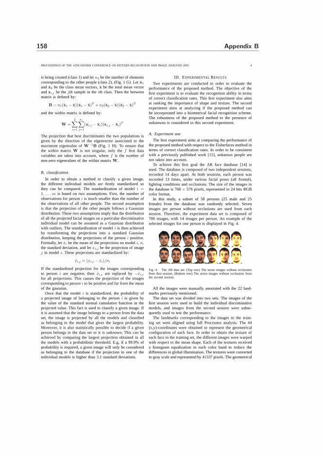
158 Appendix B
PROCEEDINGS OF THE 14TH DANISH CONFERENCE ON PATTERN RECOGNITION AND IMAGE ANALYSIS 2005 4
is being created (class 1) and letn2 be the number of elementscorresponding to the other people (class 2), (Fig. 1 G). Letx1
and x2 be the class mean vectors,x be the total mean vectorandxi,j be thejth sample in theith class. Then the betweenmatrix is defined by:
B = n1(x1 − x)(x1 − x)T + n2(x2 − x)(x2 − x)T
and the within matrix is defined by:
W =2
∑
i=1
ni∑
j=1
(xi,j − xi)(xi,j − xi)T
The projection that best discriminates the two populationsisgiven by the direction of the eigenvector associated to themaximum eigenvalue ofW−1
B (Fig. 1 H). To ensure thatthe within matrix W is not singular, only thef first datavariables are taken into account, wheref is the number ofnon-zero eigenvalues of the within matrixW.
B. classification
In order to obtain a method to classify a given image,the different individual models are firstly standardized sothey can be compared. The standardization of modeli =1, . . . , m is based on two assumptions. First, the number ofobservations for personi is much smaller than the number ofthe observations of all other people. The second assumptionis that the projection of the other people follows a Gaussiandistribution. These two assumptions imply that the distributionof all the projected facial images on a particular discriminativeindividual model can be assumed as a Gaussian distributionwith outliers. The standardization of modeli is then achievedby transforming the projections into a standard Gaussiandistribution, keeping the projections of the personi positive.Formally, letxi be the mean of the projections on modeli, σi
the standard deviation, and letxi,j be the projection of imagej in model i. These projections are standardized by:
xi,j = (xi,j − xi)/σi
If the standardized projection for the images correspondingto personi are negative, thenxi,j are replaced by−xi,j
for all projections. This causes the projection of the imagescorresponding to personi to be positive and far from the meanof the gaussian.
Once that the modeli is standardized, the probability ofa projected image of belonging to the personi is given bythe value of the standard normal cumulative function in theprojected value. This fact is used to classify a given image.Ifit is assumed that the image belongs to a person from the dataset, the image is projected by all the models and classifiedas belonging to the model that gives the largest probability.Moreover, it is also statistically possible to decide if a givenperson belongs to the data set or it is unknown. This can beachieved by comparing the largest projection obtained in allthe models with a probabilistic threshold. E.g, if a 99.9% ofprobability is required, a given image will only be consideredas belonging to the database if the projection in one of theindividual models is higher than 3.1 standard deviations.
III. E XPERIMENTAL RESULTS
Two experiments are conducted in order to evaluate theperformance of the proposed method. The objective of thefirst experiment is to evaluate the recognition ability in termsof correct classification rates. This first experiment also aimsat ranking the importance of shape and texture. The secondexperiment aims at analyzing if the proposed method canbe incorporated into a biometrical facial recognition scheme.The robustness of the proposed method to the presence ofunknowns is considered in this second experiment.
A. Experiment one
The first experiment aims at comparing the performance ofthe proposed method with respect to the Fisherfaces method interms of correct classification rates. In order to be consistentwith a previously published work [15], unknown people arenot taken into account.
To achieve this first goal the AR face database [14] isused. The database is composed of two independent sessions,recorded 14 days apart. At both sessions, each person wasrecorded 13 times, under various facial poses (all frontal),lighting conditions and occlusions. The size of the images inthe database is 768× 576 pixels, represented in 24 bits RGBcolor format.
In this study, a subset of 50 persons (25 male and 25female) from the database was randomly selected. Sevenimages per person without occlusions are used from eachsession. Therefore, the experiment data set is composed of700 images, with 14 images per person. An example of theselected images for one person is displayed in Fig. 4.
Fig. 4. The AR data set: (Top row) The seven images without occlusionsfrom first session, (Bottom row) The seven images without occlusions fromthe second session.
All the images were manually annotated with the 22 land-marks previously mentioned.
The data set was divided into two sets. The images of thefirst session were used to build the individual discriminativemodels, and images from the second session were subse-quently used to test the performance.
The landmarks corresponding to the images in the train-ing set were aligned using full Procrustes analysis. The 44(x,y)-coordinates were obtained to represent the geometricalconfiguration of each face. In order to obtain the texture ofeach face in the training set, the different images were warpedwith respect to the mean shape. Each of the textures receiveda histogram equalization in each color band to reduce thedifferences in global illumination. The textures were convertedto gray scale and represented by 41337 pixels. The geometrical

A face recognition algorithm based on MIDM 159
PROCEEDINGS OF THE 14TH DANISH CONFERENCE ON PATTERN RECOGNITION AND IMAGE ANALYSIS 2005 5
Method Input features Correct Classification Rate1
MIDM method Shape 86.4% (95)MIDM method Texture 99.6% (3)MIDM method Texture and Shape 99.9% (1)
Fishershape Shape 85.9% (99)Fisherface Texture 96.9% (22)
Fishercombined Texture and Shape 97.1% (20)
TABLE I
CORRECT CLASSIFICATION RATES.
and color representation of each face was combined, reducedand the individual models were built as described in SectionII.
The test set was used to evaluate and compare the proposedmethod with respect to the Fisherface technique. In order toevaluate the importance of the geometrical information, theFisherface technique was modified replacing the texture datawith the shape data and also combining the shape with thetexture. These two modified techniques will be referred to asFishershape and Fishercombined from now on. The EuclideanNearest-Neighbor algorithm was used as classifier algorithmin the Fisher methods. The proposed method classified theimages as the person associated to the model that yields thehighest probability.
The test was repeated a second time changing the roles ofthe training and test sets. So session two was used as trainingdata and session one as test data. The correct classificationrates for the different techniques are shown in Table I.
From Table I, it is observed that the proposed method has aslightly better performance than the Fisher methods. Moreover,it is also noticed that using the texture data one obtains a higheraccuracy than when the shape is used. This implies that theinformation contained in the texture is more significant thanthat included in the shape. However, the information containedin the shape data is not insignificant. The highest correctclassification rate in both techniques is attained when bothshape and texture are considered.
An interesting property of the proposed algorithm are thatit is possible to determine which are the most discriminativefeatures of a given person. In order to illustrate this fact,fourmodels were built using only the texture. The pixels of thefaces corresponding to these models which received the 10,15 and 25% highest weights in the model are displayed (inred) in Fig. 5. It is clear that important discriminating featuresinclude eyes, noses, glasses, moles and beards. Notice thatthealgorithm detects the glasses and the two moles of person 43as discriminate features.
B. Experiment two
The objective of this second experiment is to test the possi-bility of incorporating the proposed technique into a biometri-cal facial recognition scheme. This conveys the identificationof people in a data set and also the detection of unknownpeople. The good performance of the proposed technique inperson identification was shown in the previous experiment.
1Number of misclassified images reported in parentheses.
Fig. 5. The 10, 15 and 25% most important pixels (shown in red)fordiscriminating between the 50 test persons.
Therefore, this second experiment aims at evaluating theperformance of the technique in detection of unknown people.
To achieve this goal, the data set used in the previousexperiment is selected. In order to evaluate the performance ofthe technique, a 25-fold crossvalidation was conducted. Theseven face images from one male and other seven face imagesfrom one female were left out in each iteration. These twopeople are considered as not belonging to the data set andtherefore unknowns. The images of the remaining 48 peoplewere used to train the algorithm.
The False Acceptance Rate (FAR) and False Rejection Rate(FRR) graph, can be observed in Fig. 6. The correspondingReceiver Operating Characteristic curve (ROC) is displayed inFig. 7.
Both graphs show that the known and unknown populationshave a good separability. The best separation happens at theEqual Error Rate (3.1 standard deviations), giving a FARand FRR of 2%. Moreover, notice that, if the algorithmbelongs to a security scheme, the degree of accessibility can beestablished by increasing or diminishing the standard deviationthreshold. E.g., if in the test a false rejection rate of 5.5%isallowed, then a 0% false acceptance rate is obtained. Thisaccommodates biometrical security systems that requires ahigh level of control access.
A second test is conducted in order to assess the robustnessof the proposed method. This test also aims at showing that themethod not only discriminates on removable features, such asglasses. To achieve this goal, eight people (four male and fourfemale) are synthetically fitted with four different glasses takenfrom people belonging to the data set, giving 32 syntheticimages.
This second test consists of two steps. First, these eight

160 Appendix B
PROCEEDINGS OF THE 14TH DANISH CONFERENCE ON PATTERN RECOGNITION AND IMAGE ANALYSIS 2005 6
0 1 2 3 4 5 6 7 80
0.1
0.2
0.3
0.4
0.5
0.6
0.7
0.8
0.9
1
Confidence interval
False Acceptance RateFalse Rejection Rate
Fig. 6. False Acceptance Rate/False Rejections Rate graph obtained by the25-fold crossvalidation.
0 0.05 0.1 0.15 0.2 0.25 0.3 0.35 0.40.9
0.91
0.92
0.93
0.94
0.95
0.96
0.97
0.98
0.99
1
False positive rate (1−specificity)
Tru
e po
sitiv
e ra
te (
sens
itivi
ty)
ROC
Fig. 7. Receiver Operating Characteristic (ROC) curve obtained by the 25-fold crossvalidation. Notice that only the top left part of the ROC curve isdisplayed here.
people are not used to built the individual models. The goal isto examine if these eight people who do not belong to the dataset are considered as one of the person in the data set. Resultsshow that none of the 32 images is misclassified when athreshold of 3.1 standard deviations is considered (probabilityof correct classification of 99.9%). This fact can be noticedinFig. 8 II, where the projections of one of the eight unknownpeople on the different models are displayed. It is observedthat, when the person is considered unknown, his projectionsonto the individual models belonging to the data set are underthe selected threshold. This means that the proposed methoddoes not classify any of the unknown people as belonging tothe data set.
In the second step, the eight people (without glasses) arealso used to build the individuals models. In this case thegoal is to analyze if the method can still recognize peoplebelonging to the data set who has slight changes (same peoplewith glasses). In this second step, the 32 images are alsoclassified correctly by the method. In Fig. 8 III, it is observedthat the projections onto the individual model associated withthis person clearly surpass the threshold. It is also observedthat the projections into the individual models associatedto theglasses’s owners do not increase significantly. Similar graphs
are obtained for the other seven people. These results show thesuitability of the proposed technique in being incorporated intoa biometrical security system.
Fig. 8. Impact of changing glasses. (I) Person without glasses and syntecticfitted with 4 glasses form the data set. (II) The corresponding projections inthe models as unknown. (III) The corresponding projectionsin the models asknown. Red columns is the model corresponding to the superimposed glasses.
IV. D ISCUSSION AND CONCLUSION
In this paper, a novel method to identify people from faceimages has been proposed. The developed technique aims atbeing a precise and robust algorithm that can be incorporatedinto biometrical security systems. The technique has beentested on face images, but it can also be used in otherbiometrical data, such as speech. Experimental results haveproved that the method can attain better classifications ratesthan an other widely used technique. Moreover, the final one-dimensional projection allows for a simple interpretationof theresults. If a given face image is projected onto the differentindividual models, it is visually possible to determine if thisperson belongs to one of the models. Moreover, it is alsostatistically possible to observe the degree of belonging to thatmodel.
Another of the attracting characteristics of the proposedmethod is its ability to deal with unknowns. The degree ofbelonging to the data set can be determined statistically. Adecision threshold can be determined in relation to a standardGaussian distribution. This threshold value is used to set thedegree of security of the system. The higher this value is set,the smaller the probability of a person being considered asbelonging to the data set.
The robustness of the algorithm has been tested using bothknown and unknown people. The algorithm has been shownto be robust to the inclusion of artifacts such as glasses.On one hand, unknown people using glasses belonging topeople from the data set are still classified as unknown. Thisfact implies that unknown people would not get access toa security system when they use simple removable featuresbelonging to people from the data set. On the other hand,known people using glasses, belonging to other people fromthe data set, are still recognized as themselves. This meansifsomeone gets glasses, the associated model does not need to

A face recognition algorithm based on MIDM 161
PROCEEDINGS OF THE 14TH DANISH CONFERENCE ON PATTERN RECOGNITION AND IMAGE ANALYSIS 2005 7
be recalculated. Moreover, this fact suggests that the databaseshould be composed of facial images without glasses. This wasalso shown by observing that the individual model projectionsdo not change significantly when the glasses were placed.
Another interesting property of the proposed method is itseasiness to be maintained and updated. If a large data setis available, it is not needed to recalculate all the existingindividual models when a new person has to be registered.Simply, a new individual model for the new person is created.Similarly, if a person has to be removed from the database, itisonly needed to remove the corresponding individual model. Inconclusion, an accurate, robust and easily adaptable techniqueto be used for facial recognition has been developed anddemonstrated.
REFERENCES
[1] Statistical Shape Analysis. Wiley series in probability and statistics,1998.
[2] P.N. Belhumeur, J.P. Hespanha, and D.J. Kriegman. Eigenfaces vs.fisherfaces: Recognition using class specific linear projection. IEEETrans. Pattern Analysis and Machine Intelligence, 19(7):711–720, July1997.
[3] Hakan Cevikalp, Marian Neamtu, Mitch Wilkes, and AtalayBarkana.Discriminative common vectors for face recognition.IEEE Transactionson Pattern Analysis and Machine Intelligence, 27(1):4–13, 2005.
[4] Songcan Chen and Daohong Li. Modified linear discriminant analysis.Pattern Recognition, (38):441 443, 2005.
[5] T. F. Cootes and C. J. Taylor. Statistical models of appearance forcomputer vision. Technical report, Imaging Science and BiomedicalEngineering. University of Manchester, March 2004.
[6] I. J. Cox, J. Ghosn, and P. N. Yianilos. Feature-based face recognitionusing mixture-distance.Proceedings of IEEE Conference on ComputerVision and Pattern Recognition, pages 209–216, June 1996.
[7] J. Daugman. High confidence visual recognition of persons by a testof statistical independence.IEEE Transactions on Pattern Analysis andMachine Intelligence, 15(11):1148–1161, 1993.
[8] J. Daugman. How iris recognition works. Proceedings of 2002International Conf. on Image Processing, 1, 2002.
[9] G. Finlayson, S. Hordley, G. Schaefer, and G. Y. Tian. Illuminantand device invariant colour using histogram equalisation.PatternRecognition, 38, 2005.
[10] Xiaofei He, Shuicheng Yan, Yuxiao Hu, Partha Niyogi, and Hong-JiangZhang. Face recognition using laplacianfaces.IEEE Transactions onPattern Analysis and Machine Intelligence, 27(3):328–340, 2005.
[11] D.G. Kendall. The diffusion of shape.Advances in Applied Probabilities,(9):428–430, 1977.
[12] J. T. Kent. The complex bingham distribution and shape analysis.Proceedings in current Issues in Statistical Shape Analysis, pages 167–175.
[13] S. Z. Li and A. K. Jain.Handbook of face recognition. Springer, 2005.[14] A.M. Martinez and R. Benavente. The ar face database. Technical
Report 24, Computer Vision Center Purdue University, June 1998.[15] M. Turk and A.P. Pentland. Face recognition using eigenfaces. IEEE
Conf. Computer Vision and Pattern Recognition, 1991.[16] Ming-Hsuan Yang. Kernel eigenfaces vs. kernel fisherfaces: Face
recognition using kernel methods.Proceedings of the Fifth IEEEInternational Conference on Automatic Face and Gesture Recognition,pages 205–211, 2002.
[17] A. Yuille, P. Hallinan, and D. Cohen. Feature extraction from facesusing deformable templates.International Journal of computer Vision,1992.

162 Appendix B

Appendix C
A face recognition algorithm
based on MIDM

164 Appendix C

A face recognition algorithm based on MIDM 165
SUBMITTED - IEEE TRANSACTIONS ON PATTERN ANALYSIS AND MACHINE INTELLIGENCE - ID TPAMI-0474-0905 1
A face recognition algorithm based on multipleindividual discriminative models
David Delgado Gomez, Jens Fagertun and Bjarne K. Ersbøll
Abstract— In this paper, a novel algorithm for facial recogni-tion is proposed. The technique combines the color texture andgeometrical configuration provided by facial images. Landmarksand pixel intensities are used by Principal Component Analysisand Fisher Linear Discriminant Analysis to associate a one-dimensional projection to each person belonging to a referencedata set. Each of these projections discriminates the associatedperson with respect to all other people in the data set. Theseprojections combined with a proposed classification algorithmare able to statistically decide whether a new facial imagecorresponds to a person in the database. Each projection isalso able to visualizing the most discriminative facial featuresof the person associated to the projection. The performanceofthe proposed method is tested in two experiments. Results pointout that the proposed technique is an accurate and robust toolfor facial identification and unknown detection.
I. I NTRODUCTION
Regrettable events which happened during the last years(New York, Madrid) have revealed flaws in the existingsecurity systems. The vulnerability of most of the current se-curity and personal identification system is frequently shown.Falsification of identity cards or intrusion into physical andvirtual areas by cracking alphanumerical passwords appearfrequently in the media. These facts have triggered a realnecessity for reliable, user-friendly and widely acceptablecontrol mechanisms for person identification and verification.
Biometrics, which bases the person authentication on the in-trinsic aspects of a human being, appears as a viable alternativeto more traditional approaches (such as PIN codes or pass-words). Among the oldest biometrics techniques, fingerprintrecognition can be found. It is known that this technique wasused in China around 700 AD to officially certify contracts.Afterwards, in Europe, it was used as person identificationin the middle of the19th century. A more recent biometrictechnique used for people identification is iris recognition [9].It has been shown that the chance of finding two randomlyformed identical irises is one in1078 (The population of theearth is below1010) [8]. This technique has started to beused as an alternative to passport in some airports in UnitedKingdom, Canada and Netherlands. It is also used as employeecontrol access to restricted areas in Canadian airports andin the New York JFK airport. The inconvenience of thesetechniques is the need for interaction with the individual whowants to be identified or authenticated. This fact has causedthat face recognition, a non-intrusive technique, has increas-ingly received the interest from the scientific community inrecent years.
The first developed techniques that aimed at identifying peo-ple from facial images were based on geometrical information.
Relative distances between key points, such as mouth cornersor eyes, were calculated and used to characterize faces [19].Therefore, most of the developed techniques during the firststages of facial recognition focused on the automatic detectionof individual facial features. However, facial feature detectionand measurement techniques developed to date are not reliableenough for geometric feature based recognition, and suchgeometric properties alone are inadequate for face recognitionbecause rich information contained in the facial texture orappearance is discarded [7], [15]. This fact caused that grad-ually most of the geometrical approaches were abandoned forcolor based techniques, which provided better results. Thesemethods aligned the different faces to obtain a correspondencebetween pixels intensities. A nearest neighbor classifier usedthese aligned values to classify the different faces. This coarsemethod was notably enhanced with the appearance of theEigenfaces technique [17]. Instead of directly comparing thepixel intensities of the different face images, the dimensionof these input intensities were first reduced by principalcomponent analysis (PCA). This technique settled the basisofmany of the current image based facial recognition schemes.Among these current techniques, Fisherfaces can be found.This technique, widely used and referred [3], [5], combinestheEigenfaces with Fisher linear discriminant analysis (FLDA) toobtain a better separation of the individuals. In Fisherfaces, thedimension of the input intensity vectors is reduced by PCAand then FLDA is applied to obtain a good separation of thedifferent persons.
After Fisherfaces, many related techniques have been pro-posed. These new techniques aim at providing a projection thatattain a good person discrimination and also are robust againstdifferences in illumination or image pose. Kernel Fisherfaces[18], Laplacianfaces [12], or discriminative common vectors[4] can be found among these new approaches. Typically, thesetechniques have been tested assuming that the image to beclassified corresponds to one of the people in the database.In these approaches, the image is usually classified to theperson with the smallest Euclidean distance. However, someinconveniences appear when the person to be analyzed maynot belong to the data set. In this case, a criterium to decideifthe person belongs to the data set has to be chosen. E.g. onlypeople with an Euclidian distance less than a given thresholdare considered as belonging to the data set. However, thisthreshold does not have necessarily to be the same for allthe classes (different persons) and different thresholds wouldneed to be found. The estimation of these thresholds is notstraightforward and additional data might be needed.
In this work, a new technique that addresses these different

166 Appendix C
SUBMITTED - IEEE TRANSACTIONS ON PATTERN ANALYSIS AND MACHINE INTELLIGENCE - ID TPAMI-0474-0905 2
limitations is proposed. The proposed technique introducestwo novelties. First, not only the texture intensities are takeninto account but also the geometrical information. Second,thedata are projected inton one-dimensional spaces instead of a(n − 1)-dimensional space, wheren is the number of peoplein the data set.
Each of these individual models aims at characterizing agiven person uniquely. This means that every person in the dataset is represented by one model. These multi one-dimensionalmodels allow to statistically interpret the ”degree of mem-bership” of a person to the data set and to detect unknowns.Furthermore, these two facts have several advantages in termsof interpretability, characterization, accuracy, and easiness toupdate the model.
II. A LGORITHM DESCRIPTION
The proposed algorithm is made up of two steps. In thefirst step, an individual model is built for each person inthe database using the color and geometrical informationprovided by the available images. Each model characterizesa given person and discriminates it from the other people inthe database. The second step carries out the identification.A classifier, related with the standard Gaussian distribution,decides whether a face image belongs to one person in thedatabase or not. In this section, the two parts of the algorithmare described in detail. A diagram of the algorithm is displayedin Fig. 1. This diagram will be referred during the descriptionof the algorithm to obtain an easier understanding.
A. Creating the individual models
1) Obtaining the geometry of the face:The geometricalcharacterization of a given face is obtained by means of thetheory of statistical shape analysis [2]. In this theory, objects(faces) are represented by shapes. According to Kendall [13],a shape is all the geometrical information that remains whenlocation, scale and rotational effects are filtered out fromanobject. In order to describe a shape, a set of landmarks orpoints of correspondence that matches between and withinpopulations are placed on each face. As an example, Fig. 2Adisplays a set of 22 landmarks. These landmarks indicate theposition of the eyebrows, eyes, nose, mouth, jaw and size ofa given face.
To obtain a shape representation according to the definition,the obtained landmarks are aligned in order to remove thelocation, rotational and scaling effects. To achieve this goal,the 2D-full Procrustes analysis is carried out. Briefly, let:
X = {xi} = {xi + i · yi}, i = 1, . . . , n
be a set ofn landmarks expressed in complex notation. Inorder to apply full Procrustes analysis, the shapes are initiallycentered. To center the different shapes, the mean of the shape,x, is subtracted from each landmark:
wi = xi − x, i = 1, . . . , n
The full Procrustes mean shape [14],µ, is found as theeigenvector corresponding to the largest eigenvalue of the
Fig. 1. Algorithm overview. A: Landmarks alignment using full Procrustesanalysis. B: PCA on aligned landmarks to remove redundancy.C: Texturenormalization using global histogram equalization. D: PCAon normalizedtexture to remove redundancy. E: Combining shape and texture features. F:PCA on combined features to remove redundancy. G & H :In turn build theindividual model using FLDA.
(A) (B)
Fig. 2. (A) Set of 22 landmarks placed on a face image. (B) The Delaunaytriangulation of the 22 landmarks.

A face recognition algorithm based on MIDM 167
SUBMITTED - IEEE TRANSACTIONS ON PATTERN ANALYSIS AND MACHINE INTELLIGENCE - ID TPAMI-0474-0905 3
(A) (B)
Fig. 3. (A) Superimposition of the sets of 22 landmarks obtained over 49different face images. (B) Alignment of the landmarks.
complex sum of squares and products matrixn
∑
i=1
wiw∗
i /(w∗
i wi)
where w∗
i denotes the transpose of the complex conjugateof wi. Using this Procrustes mean shape, the full Procrustescoordinates ofw1, . . . ,wn (Fig. 1) A) are obtained by
wPi = w
∗
i µwi/(w∗
i wi) i = 1, . . . , n
Fig. 3A displays the superimposition of the set of 22landmarks described in Fig. 2, obtained on 49 different faceimages. The result obtained after applying the full Procrustesalignment on theses landmarks can be observed in Fig. 3B.In order to remove redundancy in the data, a Principal Com-ponent Analysis is applied to the aligned landmarks (Fig. 1B).
2) Texture formulation: To form a complete model ofthe face appearance, the algorithm also captures the textureinformation provided by the pixels. In order to collect thistexture representation, the Delaunay triangulation of everyshape is obtained. The Delanuay triangulation connects thealigned landmark set of each image by a mesh of triangles,so no triangle has any of the other points of the set insideits circumcircle. The Delaunay triangulation obtained foreachimage is warped onto the Delaunay triangulation of the meanshape. The Delanuay triangulation of the 22 landmarks isdisplayed in Fig. 2B.
Formally, let I be a given image andM the mean shapepreviously obtained. Letu1 = [x1, y1],u2 = [x2, y2] andu3 =[x3, y3] denote the vertices of a triangleT in I, and letv1,v2
andv3 be the associated vertices of the corresponding trianglein M . Given any internal pointu = [x, y] in the triangleT ,the corresponding point in the associated triangle in the meanshape can be written asv = αv1 + βv2 + γv3 where:
α = 1 − (β + γ)
β =yx3 − x1y − x3y1 − y3x + x1y3 + xy1
−x2y3 + x2y1 + x1y3 + x3y2 − x3y1 − x1y2
γ =xy2 − xy1 − x1y2 − x2y + x2y1 + x1y
−x2y3 + x2y1 + x1y3 + x3y2 − x3y1 − x1y2
This transformation extracts the texture of a given faceimage. A histogram equalization is applied to the collectedtexture to reduce the effects of differences in illumination [11].This histogram equalization is performed independently ineach of the three color channels. Afterwards, the three color
channels are converted into gray scale to obtain a morecompact representation (Fig. 1 C).
Similarly to the shape analysis, PCA is conducted in thetexture data to reduce dimensionality and data redundancy(Fig. 1 D). However, notice that the large dimension of thetexture vectors will produce memory problems because ofthe huge dimension of the covariance matrix. In order toavoid this difficulty, the Eckart-Young theorem is used [6].Formally, letD represents the texture data matrix composed bys n-dimensional texture vectors after the mean of the texturevectors has been subtracted from each one of them (s << n).Then then×n dimensional covariance matrix can be writtenas:
ΣD =1
sDD
T
Let ΣS be the smallers × s dimensional matrix defined by
ΣS =1
sD
TD
Then the non-zero eigenvalues of the matricesΣS and ΣD
are equal. Moreover, the columns of:
ΦD = D ·ΦS
where the columns ofΦS contain the eigenvectors ofΣS,correspond with the the eigenvectors associated to thenon-zero eigenvalues ofΣD in the sense they have the samedirection. Therefore, if the columns ofΦD are normalized,then ΦD holds the normalized eigenvectors ofΣD thathas eigenvalues bigger than zero. This does not only avoidproblems with the memory but also gives a substantialspeed-up of the calculations.
3) Combining color and geometry:Shape and texturefeatures are concatenated in a matrix (Fig. 1 E). In orderto remove correlation between shape and texture, and alsoto make the data representation more compact, a third PCAis performed on the concatenated shape and texture matrix(Fig. 1 F).
4) Building an individual model:Once the geometry andtexture of the face have been captured, the proposed algorithmbuilds an individual model for each person in the data set.Each model is built using Fisher linear discriminant analysis.Formally, letX be the data obtained after combining the shapeand texture and applying the PCA. Letn1 be the number ofdata elements corresponding to the person for whom the modelis being created (class 1) and letn2 be the number of elementscorresponding to the remaining people (class 2), (Fig. 1 G).Let x1 and x2 be the class mean vectors,x be the total meanvector andxi,j be thejth sample in theith class. Then thebetween matrix is defined by:
B = n1(x1 − x)(x1 − x)T + n2(x2 − x)(x2 − x)T
and the within matrix is defined by:
W =
2∑
i=1
ni∑
j=1
(xi,j − xi)(xi,j − xi)T
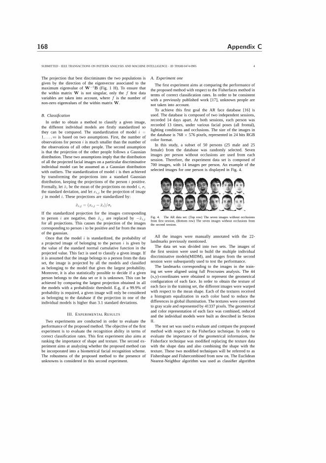
168 Appendix C
SUBMITTED - IEEE TRANSACTIONS ON PATTERN ANALYSIS AND MACHINE INTELLIGENCE - ID TPAMI-0474-0905 4
The projection that best discriminates the two populationsisgiven by the direction of the eigenvector associated to themaximum eigenvalue ofW−1
B (Fig. 1 H). To ensure thatthe within matrix W is not singular, only thef first datavariables are taken into account, wheref is the number ofnon-zero eigenvalues of the within matrixW.
B. Classification
In order to obtain a method to classify a given image,the different individual models are firstly standardized sothey can be compared. The standardization of modeli =1, . . . , m is based on two assumptions. First, the number ofobservations for personi is much smaller than the number ofthe observations of all other people. The second assumptionis that the projection of the other people follows a Gaussiandistribution. These two assumptions imply that the distributionof all the projected facial images on a particular discriminativeindividual model can be assumed as a Gaussian distributionwith outliers. The standardization of modeli is then achievedby transforming the projections into a standard Gaussiandistribution, keeping the projections of the personi positive.Formally, letxi be the mean of the projections on modeli, σi
the standard deviation, and letxi,j be the projection of imagej in model i. These projections are standardized by:
xi,j = (xi,j − xi)/σi
If the standardized projection for the images correspondingto personi are negative, thenxi,j are replaced by−xi,j
for all projections. This causes the projection of the imagescorresponding to personi to be positive and far from the meanof the gaussian.
Once that the modeli is standardized, the probability ofa projected image of belonging to the personi is given bythe value of the standard normal cumulative function in theprojected value. This fact is used to classify a given image.Ifit is assumed that the image belongs to a person from the dataset, the image is projected by all the models and classifiedas belonging to the model that gives the largest probability.Moreover, it is also statistically possible to decide if a givenperson belongs to the data set or it is unknown. This can beachieved by comparing the largest projection obtained in allthe models with a probabilistic threshold. E.g, if a 99.9% ofprobability is required, a given image will only be consideredas belonging to the database if the projection in one of theindividual models is higher than 3.1 standard deviations.
III. E XPERIMENTAL RESULTS
Two experiments are conducted in order to evaluate theperformance of the proposed method. The objective of the firstexperiment is to evaluate the recognition ability in terms ofcorrect classification rates. This first experiment also aims atranking the importance of shape and texture. The second ex-periment aims at analyzing whether the proposed method canbe incorporated into a biometrical facial recognition scheme.The robustness of the proposed method to the presence ofunknowns is considered in this second experiment.
A. Experiment one
The first experiment aims at comparing the performance ofthe proposed method with respect to the Fisherfaces method interms of correct classification rates. In order to be consistentwith a previously published work [17], unknown people arenot taken into account.
To achieve this first goal the AR face database [16] isused. The database is composed of two independent sessions,recorded 14 days apart. At both sessions, each person wasrecorded 13 times, under various facial poses (all frontal),lighting conditions and occlusions. The size of the images inthe database is 768× 576 pixels, represented in 24 bits RGBcolor format.
In this study, a subset of 50 persons (25 male and 25female) from the database was randomly selected. Sevenimages per person without occlusions are used from eachsession. Therefore, the experiment data set is composed of700 images, with 14 images per person. An example of theselected images for one person is displayed in Fig. 4.
Fig. 4. The AR data set: (Top row) The seven images without occlusionsfrom first session, (Bottom row) The seven images without occlusions fromthe second session.
All the images were manually annotated with the 22-landmarks previously mentioned.
The data set was divided into two sets. The images ofthe first session were used to build the multiple individualdiscriminative models(MIDM), and images from the secondsession were subsequently used to test the performance.
The landmarks corresponding to the images in the train-ing set were aligned using full Procrustes analysis. The 44(x,y)-coordinates were obtained to represent the geometricalconfiguration of each face. In order to obtain the texture ofeach face in the training set, the different images were warpedwith respect to the mean shape. Each of the textures receiveda histogram equalization in each color band to reduce thedifferences in global illumination. The textures were convertedto gray scale and represented by 41337 pixels. The geometricaland color representation of each face was combined, reducedand the individual models were built as described in SectionII.
The test set was used to evaluate and compare the proposedmethod with respect to the Fisherface technique. In order toevaluate the importance of the geometrical information, theFisherface technique was modified replacing the texture datawith the shape data and also combining the shape with thetexture. These two modified techniques will be referred to asFishershape and Fishercombined from now on. The EuclideanNearest-Neighbor algorithm was used as classifier algorithm
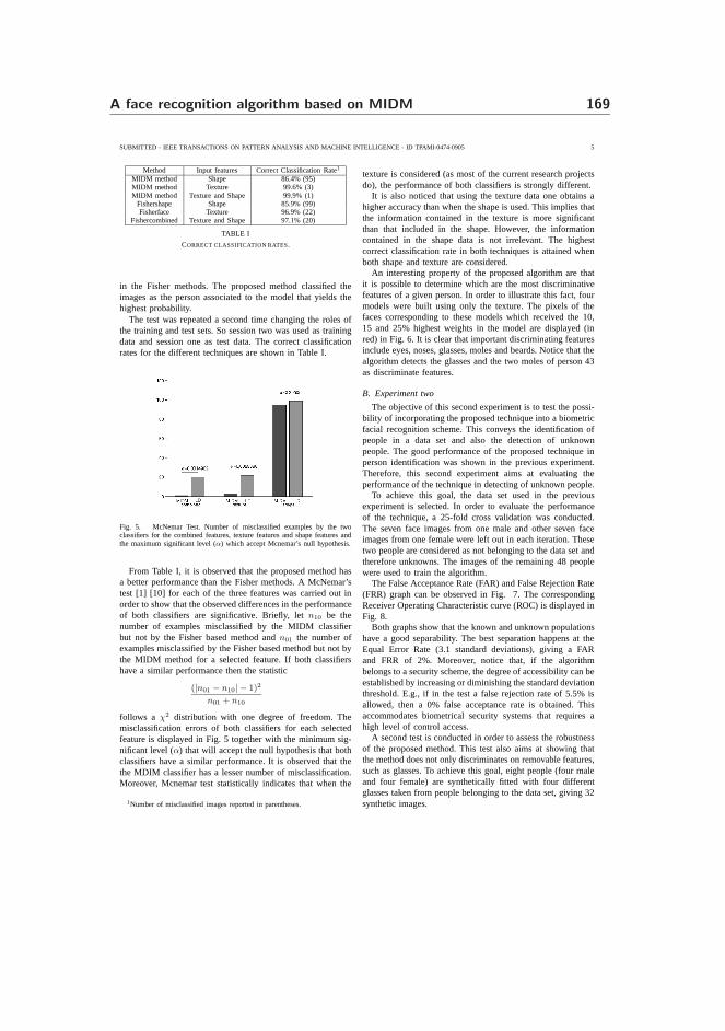
A face recognition algorithm based on MIDM 169
SUBMITTED - IEEE TRANSACTIONS ON PATTERN ANALYSIS AND MACHINE INTELLIGENCE - ID TPAMI-0474-0905 5
Method Input features Correct Classification Rate1
MIDM method Shape 86.4% (95)MIDM method Texture 99.6% (3)MIDM method Texture and Shape 99.9% (1)
Fishershape Shape 85.9% (99)Fisherface Texture 96.9% (22)
Fishercombined Texture and Shape 97.1% (20)
TABLE I
CORRECT CLASSIFICATION RATES.
in the Fisher methods. The proposed method classified theimages as the person associated to the model that yields thehighest probability.
The test was repeated a second time changing the roles ofthe training and test sets. So session two was used as trainingdata and session one as test data. The correct classificationrates for the different techniques are shown in Table I.
Fig. 5. McNemar Test. Number of misclassified examples by thetwoclassifiers for the combined features, texture features andshape features andthe maximum significant level (α) which accept Mcnemar’s null hypothesis.
From Table I, it is observed that the proposed method hasa better performance than the Fisher methods. A McNemar’stest [1] [10] for each of the three features was carried out inorder to show that the observed differences in the performanceof both classifiers are significative. Briefly, letn10 be thenumber of examples misclassified by the MIDM classifierbut not by the Fisher based method andn01 the number ofexamples misclassified by the Fisher based method but not bythe MIDM method for a selected feature. If both classifiershave a similar performance then the statistic
(|n01 − n10| − 1)2
n01 + n10
follows a χ2 distribution with one degree of freedom. Themisclassification errors of both classifiers for each selectedfeature is displayed in Fig. 5 together with the minimum sig-nificant level (α) that will accept the null hypothesis that bothclassifiers have a similar performance. It is observed that thethe MDIM classifier has a lesser number of misclassification.Moreover, Mcnemar test statistically indicates that when the
1Number of misclassified images reported in parentheses.
texture is considered (as most of the current research projectsdo), the performance of both classifiers is strongly different.
It is also noticed that using the texture data one obtains ahigher accuracy than when the shape is used. This implies thatthe information contained in the texture is more significantthan that included in the shape. However, the informationcontained in the shape data is not irrelevant. The highestcorrect classification rate in both techniques is attained whenboth shape and texture are considered.
An interesting property of the proposed algorithm are thatit is possible to determine which are the most discriminativefeatures of a given person. In order to illustrate this fact,fourmodels were built using only the texture. The pixels of thefaces corresponding to these models which received the 10,15 and 25% highest weights in the model are displayed (inred) in Fig. 6. It is clear that important discriminating featuresinclude eyes, noses, glasses, moles and beards. Notice thatthealgorithm detects the glasses and the two moles of person 43as discriminate features.
B. Experiment two
The objective of this second experiment is to test the possi-bility of incorporating the proposed technique into a biometricfacial recognition scheme. This conveys the identificationofpeople in a data set and also the detection of unknownpeople. The good performance of the proposed technique inperson identification was shown in the previous experiment.Therefore, this second experiment aims at evaluating theperformance of the technique in detecting of unknown people.
To achieve this goal, the data set used in the previousexperiment is selected. In order to evaluate the performanceof the technique, a 25-fold cross validation was conducted.The seven face images from one male and other seven faceimages from one female were left out in each iteration. Thesetwo people are considered as not belonging to the data set andtherefore unknowns. The images of the remaining 48 peoplewere used to train the algorithm.
The False Acceptance Rate (FAR) and False Rejection Rate(FRR) graph can be observed in Fig. 7. The correspondingReceiver Operating Characteristic curve (ROC) is displayed inFig. 8.
Both graphs show that the known and unknown populationshave a good separability. The best separation happens at theEqual Error Rate (3.1 standard deviations), giving a FARand FRR of 2%. Moreover, notice that, if the algorithmbelongs to a security scheme, the degree of accessibility can beestablished by increasing or diminishing the standard deviationthreshold. E.g., if in the test a false rejection rate of 5.5%isallowed, then a 0% false acceptance rate is obtained. Thisaccommodates biometrical security systems that requires ahigh level of control access.
A second test is conducted in order to assess the robustnessof the proposed method. This test also aims at showing thatthe method does not only discriminates on removable features,such as glasses. To achieve this goal, eight people (four maleand four female) are synthetically fitted with four differentglasses taken from people belonging to the data set, giving 32synthetic images.
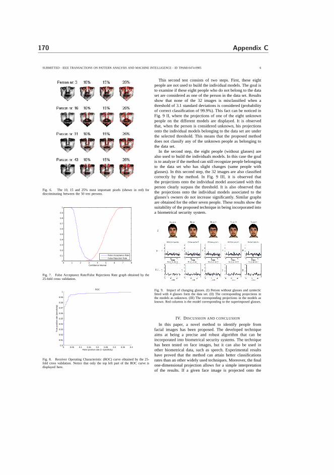
170 Appendix C
SUBMITTED - IEEE TRANSACTIONS ON PATTERN ANALYSIS AND MACHINE INTELLIGENCE - ID TPAMI-0474-0905 6
Fig. 6. The 10, 15 and 25% most important pixels (shown in red)fordiscriminating between the 50 test persons.
0 1 2 3 4 5 6 7 80
0.1
0.2
0.3
0.4
0.5
0.6
0.7
0.8
0.9
1
Confidence interval
False Acceptance RateFalse Rejection Rate
Fig. 7. False Acceptance Rate/False Rejections Rate graph obtained by the25-fold cross validation.
0 0.05 0.1 0.15 0.2 0.25 0.3 0.35 0.40.9
0.91
0.92
0.93
0.94
0.95
0.96
0.97
0.98
0.99
1
False positive rate (1−specificity)
Tru
e po
sitiv
e ra
te (
sens
itivi
ty)
ROC
Fig. 8. Receiver Operating Characteristic (ROC) curve obtained by the 25-fold cross validation. Notice that only the top left part of the ROC curve isdisplayed here.
This second test consists of two steps. First, these eightpeople are not used to build the individual models. The goal isto examine if these eight people who do not belong to the dataset are considered as one of the person in the data set. Resultsshow that none of the 32 images is misclassified when athreshold of 3.1 standard deviations is considered (probabilityof correct classification of 99.9%). This fact can be noticedinFig. 9 II, where the projections of one of the eight unknownpeople on the different models are displayed. It is observedthat, when the person is considered unknown, his projectionsonto the individual models belonging to the data set are underthe selected threshold. This means that the proposed methoddoes not classify any of the unknown people as belonging tothe data set.
In the second step, the eight people (without glasses) arealso used to build the individuals models. In this case the goalis to analyze if the method can still recognize people belongingto the data set who has slight changes (same people withglasses). In this second step, the 32 images are also classifiedcorrectly by the method. In Fig. 9 III, it is observed thatthe projections onto the individual model associated with thisperson clearly surpass the threshold. It is also observed thatthe projections onto the individual models associated to theglasses’s owners do not increase significantly. Similar graphsare obtained for the other seven people. These results show thesuitability of the proposed technique in being incorporated intoa biometrical security system.
Fig. 9. Impact of changing glasses. (I) Person without glasses and syntecticfitted with 4 glasses form the data set. (II) The corresponding projections inthe models as unknown. (III) The corresponding projectionsin the models asknown. Red columns is the model corresponding to the superimposed glasses.
IV. D ISCUSSION AND CONCLUSION
In this paper, a novel method to identify people fromfacial images has been proposed. The developed techniqueaims at being a precise and robust algorithm that can beincorporated into biometrical security systems. The techniquehas been tested on face images, but it can also be used inother biometrical data, such as speech. Experimental resultshave proved that the method can attain better classificationsrates than an other widely used techniques. Moreover, the finalone-dimensional projection allows for a simple interpretationof the results. If a given face image is projected onto the

A face recognition algorithm based on MIDM 171
SUBMITTED - IEEE TRANSACTIONS ON PATTERN ANALYSIS AND MACHINE INTELLIGENCE - ID TPAMI-0474-0905 7
different individual models, it is visually possible to determineif this person belongs to one of the models. Moreover, it isalso statistically possible to observe the degree of belongingto that model.
Another of the attractive characteristics of the proposedmethod is its ability to deal with unknowns. The degree ofbelonging to the data set can statistically be determined. Adecision threshold can be determined in relation to a standardGaussian distribution. This threshold value is used to set thedegree of security of the system. The higher this value is set,the smaller the probability of a person being considered asbelonging to the data set.
The robustness of the algorithm has been tested using bothknown and unknown people. The algorithm has been shown tobe robust to the inclusion of artifacts such as glasses. On onehand, unknown people using glasses belonging to people fromthe data set are still classified as unknown. This fact impliesthat unknown people would not get access to a security systemwhen they use simple removable features belonging to peoplefrom the data set. On the other hand, known people usingglasses, belonging to other people from the data set, are stillrecognized as themselves. This means if someone gets glasses,the associated model does not need to be recalculated.
Another interesting property of the proposed method is itseasiness to be maintained and updated. If a large data setis available, it is not needed to recalculate all the existingindividual models when a new person has to be registered.Simply, a new individual model for the new person is created.Similarly, if a person has to be removed from the database, itisonly needed to remove the corresponding individual model. Inconclusion, an accurate, robust and easily adaptable techniqueto be used for facial recognition has been developed andevaluated.
REFERENCES
[1] The analysis of contingency tables. Chapman and Hall, 1977.[2] Statistical Shape Analysis. Wiley series in probability and statistics,
1998.[3] P.N. Belhumeur, J.P. Hespanha, and D.J. Kriegman. Eigenfaces vs.
fisherfaces: Recognition using class specific linear projection. IEEETrans. Pattern Analysis and Machine Intelligence, 19(7):711–720, July1997.
[4] Hakan Cevikalp, Marian Neamtu, Mitch Wilkes, and AtalayBarkana.Discriminative common vectors for face recognition.IEEE Transactionson Pattern Analysis and Machine Intelligence, 27(1):4–13, 2005.
[5] Songcan Chen and Daohong Li. Modified linear discriminant analysis.Pattern Recognition, (38):441 443, 2005.
[6] T. F. Cootes and C. J. Taylor. Statistical models of appearance forcomputer vision. Technical report, Imaging Science and BiomedicalEngineering. University of Manchester, March 2004.
[7] I. J. Cox, J. Ghosn, and P. N. Yianilos. Feature-based face recognitionusing mixture-distance.Proceedings of IEEE Conference on ComputerVision and Pattern Recognition, pages 209–216, June 1996.
[8] J. Daugman. High confidence visual recognition of persons by a testof statistical independence.IEEE Transactions on Pattern Analysis andMachine Intelligence, 15(11):1148–1161, 1993.
[9] J. Daugman. How iris recognition works. Proceedings of 2002International Conf. on Image Processing, 1, 2002.
[10] T. G. Dietterich. Approximate statistical tests for comparing supervisedclassification learning algorithms.Neural Computation, pages 1895–1923, 1998.
[11] G. Finlayson, S. Hordley, G. Schaefer, and G. Y. Tian. Illuminantand device invariant colour using histogram equalisation.PatternRecognition, 38, 2005.
[12] Xiaofei He, Shuicheng Yan, Yuxiao Hu, Partha Niyogi, and Hong-JiangZhang. Face recognition using laplacianfaces.IEEE Transactions onPattern Analysis and Machine Intelligence, 27(3):328–340, 2005.
[13] D.G. Kendall. The diffusion of shape.Advances in Applied Probabilities,(9):428–430, 1977.
[14] J. T. Kent. The complex bingham distribution and shape analysis.Proceedings in current Issues in Statistical Shape Analysis, pages 167–175.
[15] S. Z. Li and A. K. Jain.Handbook of face recognition. Springer, 2005.[16] A.M. Martinez and R. Benavente. The ar face database. Technical
Report 24, Computer Vision Center Purdue University, June 1998.[17] M. Turk and A.P. Pentland. Face recognition using eigenfaces. IEEE
Conf. Computer Vision and Pattern Recognition, 1991.[18] Ming-Hsuan Yang. Kernel eigenfaces vs. kernel fisherfaces: Face
recognition using kernel methods.Proceedings of the Fifth IEEEInternational Conference on Automatic Face and Gesture Recognition,pages 205–211, 2002.
[19] A. Yuille, P. Hallinan, and D. Cohen. Feature extraction from facesusing deformable templates.International Journal of computer Vision,1992.

172 Appendix C

Appendix D
FaceRec Quick User Guide

174 Appendix D
When opening FaceRec one has to select a video driver from which the videoinput will be received. This is displayed in Figure D.1 and Figure D.2.
Figure D.1: The main window of the FaceRec application. Go to themenu “Video” -> “Capture WebCam Drivers” to select the video driver.
Figure D.2: The video driver list popup box.
It is possible to adjust the video feed (webcam) by activating the “Video Source”,“Video Format”, “Video Display” and “Video Compression” panel from the“Video” menu, if these are available in the selected video driver (available are de-noted by black selectable items and non-available by gray non-selectable items).An example of a Philips PCVC690K webcam “Video Source” panel is displayedin figure D.3.
FaceRec is processing the face detection and face recognition in real time whenboth an AAM Model File (.amf) and an MIDM Model File (.mmf) are loaded,as displayed in figure D.4.
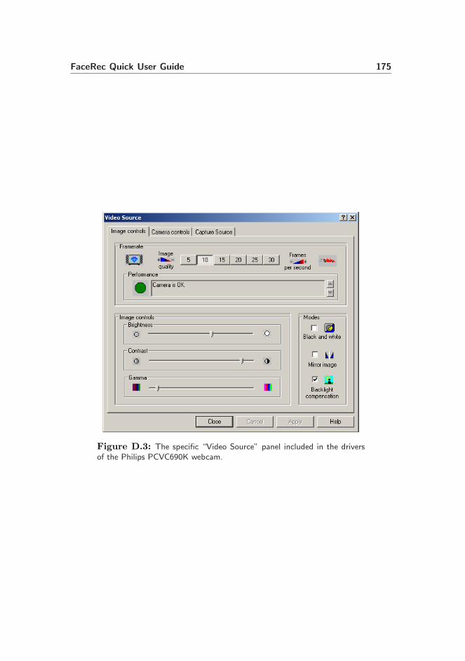
FaceRec Quick User Guide 175
Figure D.3: The specific “Video Source” panel included in the driversof the Philips PCVC690K webcam.
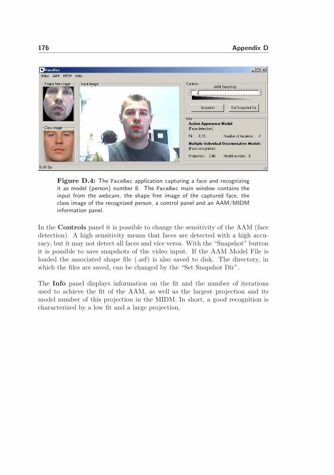
176 Appendix D
Figure D.4: The FaceRec application capturing a face and recognizingit as model (person) number 8. The FaceRec main window contains theinput from the webcam, the shape free image of the captured face, theclass image of the recognized person, a control panel and an AAM/MIDMinformation panel.
In the Controls panel it is possible to change the sensitivity of the AAM (facedetection). A high sensitivity means that faces are detected with a high accu-racy, but it may not detect all faces and vice versa. With the “Snapshot” buttonit is possible to save snapshots of the video input. If the AAM Model File isloaded the associated shape file (.asf) is also saved to disk. The directory, inwhich the files are saved, can be changed by the “Set Snapshot Dir”.
The Info panel displays information on the fit and the number of iterationsused to achieve the fit of the AAM, as well as the largest projection and itsmodel number of this projection in the MIDM. In short, a good recognition ischaracterized by a low fit and a large projection.

Appendix E
AAM-API DLL

178 Appendix E
DLL index Function name Short description
#1 deleteImage Deletes the AAM image object#2 deleteModel Deletes the AAM model object#3 deleteReferenceFrame Deletes the AAM reference frame
object#4 deleteShape Deletes the AAM shape object#5 evalShape Manipulates the AAM shape to
find a the best fit using a AAMmodel object and a AAM imageobject
#6 evalShapeFineTuning Manipulates the AAM shape tofind a the best fit using a AAMmodel object and a AAM imageobject
#7 getNCombinedPCA Returns the number of combinedpca parameters of a AAM modelobject
#8 getNTextureSamples Returns the number of texturesamples in the shape free imageof a AAM model object
#9 getShape Returns the shape coordinates#10 getShapeBox Returns the coordinates for the
box the AAM shape object re-sides in
#11 getShapeFreeImage Returns the shape free image of aAAM shape object, AAM imageobject and AAM model object
#12 initializeShape Initialize a AAM shape object
Table E.1: Function list over the aam api.dll.

AAM-API DLL 179
DLL index Function name Short description
#13 modelImage Models a face (object) using thecombined PCA parameters ontoan AAM image object
#14 newImage Constructs a new AAM imageobject
#15 newModel Constructs a new AAM modelobject
#16 newReferenceFrame Constructs a new AAM referenceframe object
#17 newShape Constructs a new AAM shapeobject
#18 readImage Reads an image from a char ar-ray into an AAM image object
#19 readModel Reads an AAM model objectfrom file
#20 shapeCOG Returns the center of gravity ofan AAM shape object
#21 translateShape Translates an AAM shape object#22 writeASF Writes an AAM shape object to
file#23 writeImage Writes an image from an AAM
image object into a char array
Table E.2: Function list over the aam api.dll continued.

180 Appendix E

Appendix F
CD-ROM Contents

182 Appendix F
Figure F.1: The contents of the enclosed CD-ROM.

Bibliography
[1] Jorgen Ahlberg. Model-based Coding: Extraction, Coding, and Evaluationof Face Model Parameters. PhD thesis, Department of Electrical Engineer-ing, Linkoping University, 2002.
[2] M. Aizerman, E. Braverman, and L. Rozonoer. Theoretical foundations ofthe potential function method in pattern recognition learning. Automationand Remote Control, 25:821–837, 1964.
[3] G. Baudat and F. Anouar. Generalized discriminant analysis using a kernelapproach. Neural Computation, pages 2385–2404, 2000.
[4] P. N. Belhumeur, J. P. Hespanha, and D. J. Kriegman. Eigenfaces vs.Fisherfaces: Recognition using class specific linear projection. IEEE Trans.Pattern Analysis and Machine Intelligence, 19(7):711–720, July 1997.
[5] M. Bichsel and A. Pentland. Human face recognition and the face im-age set’s topology. Computer Vision, Graphics, and Image Processing,59(2):254–261, 1994.
[6] I. Biederman and P. Kalocsai. Neurocomputational bases of objectand face recognition. Philosophical Transactions: Biological Sciences,352(1358):1203–1219, 1997.
[7] H. Cevikalp, M. Neamtu, M. Wilkes, and A. Barkana. Discriminative com-mon vectors for face recognition. IEEE Transactions on Pattern Analysisand Machine Intelligence, 27(1):4–13, 2005.
[8] D. Chandler. Visual perception. Internet site (Link :http://www.aber.ac.uk/media/Modules/MC10220/visindex.html).

184 BIBLIOGRAPHY
[9] S. Chen and D. Li. Modified linear discriminant analysis. Pattern Recog-nition, pages 441–443, 2005.
[10] T. F. Cootes and C. J. Taylor. Statistical models of appearance for com-puter vision. Technical report, Imaging Science and Biomedical Engineer-ing. University of Manchester, March 2004.
[11] T. F. Cootes, C. J. Taylor, D. H. Cooper, and J. Graham. Active shapemodels - their training and application. Computer Vision and Image Un-derstanding, 61(1):38–59, 1995.
[12] I. J. Cox, J. Ghosn, and P. N. Yianilos. Feature-based face recognition usingmixture-distance. Proceedings of IEEE Conference on Computer Visionand Pattern Recognition, pages 209–216, June 1996.
[13] I. Craw, D. Tock, and A. Bennett. Finding face features. Proc. SecondEuropean Conf. Computer Vision, pages 92–96, 1992.
[14] Y. Dai and Y. Nakano. Face-texture model based on SGLD and its appli-cation in face detection in a color scene. Pattern Recognition, 29(6):1007–1017, 1996.
[15] C. Darwin. The Expression of the Emotions in Man and Animals. London:John Murray, 1872.
[16] B. V. Dasarathy. Nearest Neighbor (NN) Norms : Nn Pattern ClassificationTechniques. IEEE Computer Society Press, 1991.
[17] J. Daugman. How iris recognition works. Proceedings of 2002 InternationalConf. on Image Processing, 1, 2002.
[18] I. Dryden and K. V. Mardia. Statistical Shape Analysis. Wiley series inprobability and statistics, 1998.
[19] B. K. Ersbøll and K. Conradsen. An introduction to statistics, volume 2.DTU-tryk, 2003.
[20] J. Fagertun, D. D. Gomez, B. K. Ersbøll, and R. Larsen. A face recognitionalgorithm based on multiple individual discriminative models. Proceedingsof the 14th Danish Conference on Pattern Recognition and Image Analysis,2005.
[21] J. Fagertun and M. B. Stegmann. The IMM frontal face database. TechnicalReport 11, Informatics and Mathematical Modelling, Technical Universityof Denmark, DTU, Richard Petersens Plads, Building 321, DK-2800 Kgs.Lyngby, aug 2005.
BIBLIOGRAPHY 185
[22] G. Finlayson, S. Hordley, G. Schaefer, and G. Y. Tian. Illuminant anddevice invariant colour using histogram equalisation. Pattern Recognition,38, 2005.
[23] M. A. Fischler and R. A. Elschlager. The representation and matching ofpictorial structures. IEEE Transactions on Computers, 22(1):67–92, 1973.
[24] F. Galton. Personal identification and description. Nature, pages 173–188,1888.
[25] I. Gauthier and M. Behrmann. Can face recognition really be dissociatedfrom object recognition? Journal of Cognitive Neuroscience, 11(4), 1999.
[26] A. J. Goldstein and L. D. Harmon. Identification of human faces. Proceed-ings of the IEEE, pages 748–760, 1971.
[27] D. D. Gomez, J. Fagertun, and B. K. Ersbøll. A face recognition algorithmbased on multiple individual discriminative models. IEEE Transactions onPattern Analysis and Machine Intelligence, 2005. To appear, Submitted in2005, ID TPAMI-0474-0905.
[28] C. Goodall. Procrustes methods in the statistical analysis of shape. Journalof the Royal Statistical Society, 53(2):285–339, 1991.
[29] X. He and P. Niyogi. Locality preserving projections. Proc. Conf. Advancesin Neural Information Provessing Systems, 2003.
[30] X. He, S. Yan, Y. Hu, P. Niyogi, and H. Zhang. Face recognition usingLaplacianfaces. IEEE Transactions on Pattern Analysis and Machine In-telligence, 27(3):328–340, 2005.
[31] R. Heindl. System und Praxis der Daktyloskopie und der sonstigen technis-chen Methoden der Kriminalpolizei. De Gruyter, Berlin, 1922.
[32] R. Hietmeyer. Biometric identification promises fast and secure process-ing of airline passengers. The International Civil Aviation OrganizationJournal, 55(9):10–11, 2000.
[33] D. G. Kendall. The diffusion of shape. Advances in Applied Probabilities,pages 428–430, 1977.
[34] R. Kjeldsen and J. Kender. Finding skin in color images. Proc. SecondInternational Conf. Automatic Face and Gesture Recognition, pages 312–317, 1996.
[35] A. Lanitis, C. J. Taylor, and T. F. Cootes. An automatic face identificationsystem using flexible appearance models. Image and Vision Computing,13(5):393–401, 1995.
186 BIBLIOGRAPHY
[36] T. K. Leung, M. C. Burl, and P. Perona. Finding faces in cluttered scenesusing random labeled graph matching. Proc. Fifth IEEE InternationalConf. Computer Vision, pages 637–644, 1995.
[37] S. Z. Li and A. K. Jain. Handbook of face recognition. Springer, 2005.
[38] Q. Liu, R. Huang, H. Lu, and S. Ma. Face recognition using kernel-basedfisher discriminant analysis. Proceedings Fifth IEEE International Confer-ence on Automatic Face Gesture Recognition, pages 197–201, 2002.
[39] J. Luettin and G. Maıtre. Evaluation protocol for the extended M2VTSdatabase (lausanne protocol). IDIAP Communication 98-05, 1998.
[40] A. M. Martinez. PCA versus LDA. IEEE Transactions on Pattern Analysisand Machine Intelligence, 23(2):228–233, 2001.
[41] A. M. Martinez and R. Benavente. The AR face database. TechnicalReport 24, Computer Vision Center (CVC), June 1998.
[42] K. Messer, J. Kittler, M. Sadeghi, S. Marcel, C. Marcel, S. Bengio, F. Car-dinaux, C. Sanderson, J. Czyz, L. Vandendorpe, S. Srisuk, M. Petrou,W. Kurutach, A. Kadyrov, R. Paredes, B. Kepenekci, F. B. Tek, G. B. Akar,F. Deravi, and N. Mavity. Face verification competition on the XM2VTSdatabase. Audio- and Video-Based Biometric Person Authentication. 4thInternational Conference, AVBPA 2003, 2003.
[43] K. Messer, J. Matas, J. Kittler, J. Luttin, and G. Maitre. XM2VTSDB: Theextended M2VTS database. In Audio- and Video-based Biometric PersonAuthentication, AVBPA’99, pages 72–77, 1999. Washington, D.C., March1999. 16 IDIAP–RR 99-02.
[44] S. Mika, G. Ratsch, J. Weston, B. Scholkopf, and K. R. Mullers. Fisher dis-criminant analysis with kernels. Neural Networks for Signal Processing IX,1999. Proceedings of the 1999 IEEE Signal Processing Society Workshop,pages 41–48, 1999.
[45] P. J. Phillips, P. Grother, R. J. Micheals, D. M. Blackburn, E. Tabassi, andM. Bone. Face recognition vendor test 2002. Technical report, NationalInstitute of Standards and Technology, March 2003.
[46] F. P. Preparata and M. I. Shamos. Computational Geometry: An Intro-duction. Springer, 1985.
[47] H. Rowley, S. Baluja, and T. Kanade. Neural network-based face detec-tion. IEEE Transactions on Pattern Analysis and Machine Intelligence,20(1):23–38, 1998.
BIBLIOGRAPHY 187
[48] H. Rowley, S. Baluja, and T. Kanade. Rotation invariant neural network-based face detection, 1998.
[49] K. Skoglund. Three-dimensional face modelling and analysis. Master’sthesis, Informatics and Mathematical Modelling, Technical University ofDenmark, DTU, Richard Petersens Plads, Building 321, DK-2800 Kgs.Lyngby, 2003. Supervised by Assoc. Prof. Rasmus Larsen.
[50] M. B. Stegmann. Active appearance models theory extensions and cases.Master’s thesis, Technical University of Denmark, 2000.
[51] M. B. Stegmann, B. K. Ersbøll, and R. Larsen. FAME - a flexible ap-pearance modelling environment. IEEE Transactions on Medical Imaging,22(10):1319–1331, 2003.
[52] F. Sukno, S. Ordas, C. Butakoff, S. Cruz, and A. Frangi. Active shapemodels with invariant optimal features IOF-ASMs. In Proceedings of Audio-and Video-Based Biometric Person Authentication, pages 365–375, NewYork, USA, 2005. Springer.
[53] M. Turk. A random walk through eigenspace. IEICE Trans. Inf. & Syst.,E84-D(12):1586–1595, December 2001.
[54] M. Turk and A. Pentland. Eigenfaces for recognition. J. Cognitive Neu-rosicence, 3(1):71–86, 1991.
[55] M. Turk and A. P. Pentland. Face recognition using eigenfaces. IEEE Conf.Computer Vision and Pattern Recognition, 1991.
[56] X. Xie and K. M. Lam. Face recognition under varying illumination basedon a 2dface shape model. Pattern Recognition, 38:211–230, 2005.
[57] G. Yang and T. S. Huang. Human face detection in complex background.Pattern Recognition, 27(1):53–63, 1994.
[58] J. Yang and A. Waibel. A real-time face tracker. Proc. Third WorkshopApplications of Computer Vision, pages 142–147, 1996.
[59] M. H. Yang. Kernel Eigenfaces vs. Kernel Fisherfaces: Face recognition us-ing kernel methods. Proceedings of the Fifth IEEE International Conferenceon Automatic Face and Gesture Recognition, pages 205–211, 2002.
[60] M. H. Yang, D. J. Kriegman, and N. Ahuja. Detecting faces in images: Asurvey. IEEE Transactions on Pattern Analysis and Machine Intelligence,24(1):34–58, January 2002.
[61] A. Yuille, P. Hallinan, and D. Cohen. Feature extraction from faces usingdeformable templates. International Journal of computer Vision, 1992.


