
Report Prepared by:
Alberto A. Sagiif!s S.C. Krane A.K.M. AI-Mansur Sherry Hierholzer
FACTORS CONTROLLING CORROSION OF STEEL-REINFORCED CONCRETE
SUBSTRUCTURE IN SEAWATER
Final Report to Florida D.O.T. WPI No. 0510537, State Job No. 99700-7530-119
Alberto A. Sagues, P .I. Department of Civil Engineering and Mechanics
College of Engineering University of South Florida
Tampa, Florida 33620-5350 December, 1994

1. Report No.
FL/DOT/RC/0537-3523 I 2. Government Accoosion No.
4. Title and Subtitle
FACTORS CONTROLLING CORROSION OF STEELREINFORCED CONCRETE SUBSTRUCTURE IN SEA WATER
7. Author's
Alberto A. Sagues, S.C. Krane, A.K.M. Al-Mansur, S. Hierholzer
9. Performing Organization Name and Address
Department of Civil Engineering and Mechanics University of South Florida Tampa, FL 33620
12. Sponsoring Agency Name and Address
Florida Department of Transportation Materials Office P.O. Box 1029 Gainesville, FL 32602
15. Supplementary Notes
Prepared in cooperation with the Federal Highway Administration
16. Abstract
Technical Report Documentatwn Page 3. Recipient's Catalog No.
6. Report Date
December, 1994
6. Performing Organization Code
8. Performing Organization Report No.
10. Work Unit No. ITRAISI
11. Coolract or Grant No.
WPI 0510537
13. Typo of Report and Period Covered
Final Report September 1990- December 1993
14. Sponsoring Agency Code
Laboratory experiments and computer model calculations were performed to assess the effect of critical design variables and concrete properties on the distribution of corrosion in reinforced concrete marine bridge substructures. Instrumented laboratory test columns were exposed for a period of three years in conditions simulating field service. One set of columns was made with concrete containing fly ash, concrete with fly ash plus silica fume, and concrete with either silane or siloxane surface treatments. This set was prepared for evaluation of the effects of concrete composition and surface treatments on corrosion distribution. From concrete resistivity measurements, the concrete with fly ash plus silica fume showed evidence of having the lowest permeability at early test ages (first two years), but the differences between both types of concrete tended to be less near the end of the test. Both surface treatments tended to reduce the intake of water but did not cause excessive water retention. Another set of columns was made with concrete without pozzolanic additions, and used to evaluate the effect of partial and saturating moisture application in the region above the waterline. Corrosion macrocell measurements indicated that cathodic activity (and macrocell action) increased with partial moisture application but reached a limiting amount upon saturation. The behavior was linked to diffusional transport limitation of the oxygen reduction reaction. The computer calculations produced a comprehensive model to predict corrosion current distribution. The predicted corrosion was greatest at the top of the active steel zone in the reinforcement assembly. The calculations indicated than the diffusivity of oxygen in the concrete was relatively more important than concrete resistivity in determining the overall extent of corrosion. Applications of the findings to design of future structures are proposed.
17. Key Words 18. Distributioo Statcmont
Reinforcing Steel, Corrosion, Rebar, Concrete, Computation No restrictions. This document is available to the public through the National Technical Information Service, Springfield, VA 22161
19. Security Clasoif.(of this report)
Unclassified 1
20. Security Classif. (of this page)
Unclassified 21. No. of Pages
115 22. Prioe
onn DOT F 17UU.7 (lS-72)
Reproduction of completed page authorized

METRIC CONVERSION FACTORS
CONVERI' TO MUili.'IPLY BY
l. LENGIH inch mm 25.4 foot mm 304.8 yard meter 0. 9144 IllE!.ter foot 3.281 meter inch 39.37
2. FORCE pound (lb) newton (N) 4.448 kip ( 1000 lb) kilo newton (kN) 4.448 newton (N) pound (lb) 0.225 kilo newton (kN) kipk 0.225
3. FORCE/ kip/ft kN/m 14.59 I.ENGIH kN/rn lb/ft 68.52
kN/rn kipjft 0.0685
4. STRESS pound/in2 (psi) N/mm2 (MPa) 0.0069
kipsjin2 (ksi) N/mm2 (MPa) 6.895
newton;mm2 ksi 0.145
5. MCMENTS ft-kip kN-rn 1.356 in.:.. kip kN-rn 0.1l3 kN-rn ft-kip 0. 7375.
ii

CREDITS/DISCLAIMER
This report was prepared in cooperation with the State of Florida
Department of Transportation (FDOT) and the U.S. Department of Transportation.
The Corrosion Section of the Materials Office, Florida Department of
Transportation, Gainesville, Florida provided valuable assistance in the preparation
of concrete laboratory specimens and analysis of concrete samples. The opinions,
findings and conclusions expressed in this publication are those of the authors
and not necessarily those of the State of Florida Department of Transportation or
the U.S. Department of Transportation.
iii

TABLE OF CONTENTS
ABSTRACT .......................................... .
METRIC CONVERSION TABLE . . . . . . . . . . . . . . . . . . . . . . . . . . . . . . ii
CREDITS/DISCLAIMER . . . . . . . . . . . . . . . . . . . . . . . . . . . . . . . . . . . . iii
EXECUTIVE SUMMARY . . . . . . . . . . . . . . . . . . . . . . . . . . . . . . . . . . . 1
1. INTRODUCTION . . . . . . . . . . . . . . . . . . . . . . . . . . . . . . . . . . . . 4
2. APPROACH . . . . . . . . . . . . . . . . . . . . . . . . . . . . . . . . . . . . . . . 5
3. PART 1: EXPERIMENTAL INVESTIGATION OF THE EFFECT OF
CONCRETE COMPOSITION AND SURFACE TREATMENT
3.1 PROCEDURE . . . . . . . . . . . . . . . . . . . . . . . . . . . . . . . . . 7
3.2 RESULTS AND DISCUSSION . . . . . . . . . . . . . . . . . . . . . . . 12
3.3 REFERENCES . . . . . . . . . . . . . . . . . . . . . . . . . . . . . . . . . 23
3.4 TABLE . . . . . . . . . . . . . . . . . . . . . . . . . . . . . . . . . . . . . . 25
3.5 FIGURES . . . . . . . . . . . . . . . . . . . . . . . . . . . . . . . . . . . . Fl-1
4. PART II: EFFECT OF CONCRETE MOISTURE
4.1 PROCEDURE . . . . . . . . . . . . . . . . . . . . . . . . . . . . . . . . . 26
4.2 RESULTS AND DISCUSSION . . . . . . . . . . . . . . . . . . . . . . . 28
4.3 REFERENCES . . . . . . . . . . . . . . . . . . . . . . . . . . . . . . . . . 34
4.4 FIGURES . . . . . . . . . . . . . . . . . . . . . . . . . . . . . . . . . . . . Fll-1
5. PART Ill: CORROSION DISTRIBUTION MODELLING
5.1 BACKGROUND . . . . . . . . . . . . . . . . . . . . . . . . . . . . . . . . 35
5.2 APPROACH . . . . . . . . . . . . . . . . . . . . . . . . . . . . . . . . . . 38
5.3 RESULTS AND DISCUSSION . . . . . . . . . . . . . . . . . . . . . . . 44
5.4 NOMENCLATURE . . . . . . . . . . . . . . . . . . . . . . . . . . . . . . 56
5. 5 REFERENCES . . . . . . . . . . . . . . . . . . . . . . . . . . . . . . . . . 58
5.6 TABLES . . . . . . . . . . . . . . . . . . . . . . . . . . . . . . . . . . . . . 60
5.7 FIGURES . . . . . . . . . . . . . . . . . . . . . . . . . . . . . . . . . . . . Flll-1
6. GENERAL DISCUSSION . . . . . . . . . . . . . . . . . . . . . . . . . . . . . . 62
7. CONCLUSIONS . . . . . . . . . . . . . . . . . . . . . . . . . . . . . . . . . . . . 63
8. STATEMENT OF BENEFITS . . . . . . . . . . . . . . . . . . . . . . . . . . . . 68
iv

EXECUTIVE SUMMARY
Reinforcement corrosion severely limits the service life of concrete exposed to
seawater. To achieve extended design service life, it is important to quantitatively
assess the relative importance of design parameters such as concrete composition,
concrete properties, structural dimensions and concrete surface treatments. To that
effect, this three-part investigation examined selected factors that control the corrosion
of reinforcing steel in the substructure of marine bridges.
The first part of the investigation had the objective of examining the effect of
concrete composition and surface treatment on the development of corrosion. This
objective was addressed experimentally by constructing instrumented reinforced
concrete columns and placing them in a laboratory salt water tank simulating
submerged, splash, and atmospheric exposure regions. The concrete compositions
used reflect current and near-future Florida DOT design: F specimens {Type II
cement with 20% Fly Ash replacement) , and F+S specimens (20% Fly Ash and 5%
Microsilica). The concrete surface treatments used were Silane and Siloxane, applied
to the above-water portion of the test columns. Testing took place over a 3-year
period. The columns developed concrete resistivity patterns representative of those
encountered in the field. The resistivity results indicated that both concrete surface
treatments prevented water ingress but did not cause water to be retained to the
extent that unwanted enhancement of corrosion macrocell action would have taken
place. The resistivity results for the zones below water and corrosion macrocell
current measurements indicated that the F concrete was initially significantly more
permeable than the F+S concrete, but the differences between both types of concrete
tended to become much less pronounced as time progressed. The effect, which
resulted in comparable behavior for both mixes after about two years of exposure, was
ascribed to the maturing of the pozzolan ic reaction during that period in the F
specimens. It was concluded that future assessment of the relative merits of mixtures
with and without microsilica give special attention to long term field experience.
1

Corrosion macrocell patterns in the test columns had began to reach maturity by the
end of the project, and continued testing is planned for the future.
The second part of the investigation had the objective of establishing the
extent of corrosion macrocell action and its variation with concrete moisture in marine
substructure service. This objective was addressed also using laboratory columns
partially submerged in salt water. The column geometry allowed for detailed
separation of the reinforcing steel into individual elements. Only one concrete, with
Type I cement, was used. The evolution of corrosion was followed for a period of 3
years as a function of time and of the degree of moisturizing of the above-water
portion of the columns. The cathodic current in the upper portion of the columns was
increased upon partial moisturizing, as a result of the reduction of ohmic potential
drops in the corrosion macrocell system. However, as the region above water was
moisturized to saturation, the cathodic current did not increase proportionally but
reached a limiting value consisting with concentration polarization of the cathodic
reaction. The value of the limiting current density in saturated concrete corresponded
to an effective diffusion coefficient for oxygen in concrete of 6 1 o·6 cm2/sec, in
agreement with values independently reported in the literature.
The objective of the third part of the investigation was to develop a
comprehensive model for the prediction of corrosion distribution in reinforced concrete
piling as a function of concrete properties and system geometry. A computational
model was developed for a generic substructure column using finite difference
calculations. The distributions of electric potential and oxygen concentration were
calculated for the corrosion propagation stage. The concrete resistivity and oxygen
diffusivity distribution profiles of the column were used as inputs. The model provided
quantitative prediction of the resulting corrosion rate along the reinforcement cage.
The concentration of oxygen inside the column was found to vary from a value near
equilibrium with the exterior at the top, to almost zero below water. Oxygen transport
to the steel below water was almost exclusively through the concrete cover and not
2

downward through the center of the column. The corrosion current density was
greatest at the top of the active zone of the column. Corrosion below water
proceeded at a smaller rate even though the steel potential was significantly less
noble than in the region of highest corrosion. The overall level of corrosion increased
with increasing oxygen diffusivity and reduced concrete resistivity. However, the
relative changes in oxygen diffusivity had the greatest impact on corrosion activity.
The different approaches of the investigation confirmed the importance of
corrosion macrocells in the development of corrosion in macrocell columns. Oxygen
transport was a critical factor in determining corrosion severity. Design that promotes
moist concrete conditions {as in submerged substructure footers) is recommended as
a corrosion prevention/control approach. Concrete resistivity is another critical
variable. Monitoring of concrete resistivity is recommended not only as a gage of
possible corrosion severity, but also in moist specimens as an additional indicator of
overall concrete quality.
3

1. INTRODUCTION
The substructure of reinforced concrete bridges over marine waters in Florida is
subject to damage due to corrosion of the reinforcing steel. The steel reinforcing bars
(rebars) are initially protected by the alkaline nature of the surrounding concrete.
However, chloride ions from the seawater accumulate on the surface of the concrete
and slowly migrate through the concrete cover to the underlying steel. When the
chloride ion concentration at the rebar depth exceeds a critical threshold value, the
protective passive layer on the steel surface breaks down and active corrosion of the
steel begins. The corrosion products occupy a volume that can be several times
larger than that of the initial steel, thus causing cracks of the concrete cover with
consequent structural damage.
The time period from construction until the beginning of active rebar corrosion is
called the initiation stage of the corrosion process. The following period from
beginning of active corrosion until appearance of external manifestation of structural
damage (cracking, rust, spalling) is called the propagation stage. This investigation
was aimed primarily at determining the relative importance of design and service
factors on the extent of corrosion experienced during the propagation stage in marine
substructures of Florida bridges. The factors selected for examination concerned
parameters that can be affected by the outcome of decisions presently being made by
the Florida Department of Transportation (FOOT) on concrete mix design and
structural dimensioning. These parameters include the extent of pozzolanic additions
(fly ash and microsilica) to the concrete mix, concrete surface treatments, the physical
dimensions of the substructure, and the extent of concrete wetting that can result in
service. These parameters are expected to affect the electrical resistivity and oxygen
diffusivity of the concrete. Prior to this investigation, there was qualitative agreement
that corrosion was less severe when concrete resistivity was greater, and that
corrosion macrocells played a significant role on the extent and distribution of
corrosion of rebar in concrete. However, relatively little was known about the value of
4

these parameters and their relative importance in Florida substructures. There was
also no quantitative treatment to serve as a tool to investigate the effect of changes in
the relevant variables on the overall corrosion extent and distribution. The
investigation described here addressed those matters by establishing the objectives
indicated below.
1.1 OBJECTIVES
(1) Examine the effect of selected concrete compositions and surface treatments
on the development of corrosion in marine substructure.
(2) Establish the extent of corrosion macrocell action and its variation with concrete
moisture in marine substructure service.
(3) Develop a comprehensive model for the prediction of corrosion distribution in
reinforced concrete piling as a function of concrete properties and system geometry.
2. APPROACH
The first objective, the effect of concrete composition and surface treatment,
was addressed experimentally by constructing reinforced concrete columns and
placing them in a salt water tank with the lower portion of each column submerged.
Periodic salt-water wetting of the portion of each column just above water replicated
the splash-evaporation regime encountered in the field. The reinforcement in each
column was split electrically to allow measurement of macrocell currents and overall
corrosion activity as a function of time. The baseline column contained concrete made
with Type II cement and 20% fly ash replacement. Variations included the addition of
5% microsilica, and the use of silane or siloxane surface treatments on the portion of
the columns above water. Testing took place for for nearly 3 years.
5

The second objective, the determination of macrocell action and effect of
moisture, was also addressed using laboratory columns partially submerged in salt
water. The geometry of these columns allowed for more detailed separation of the
reinforcing steel into individual elements. The only concrete formulation used was
Type I cement with no pozzolanic additions. The evolution of corrosion in these
systems was evaluated as a function of time, and the upper portion of selected
columns was subject to fresh-water wetting to cause pronounced variations in the
concrete resistivity profile. This testing also took place for nearly 3 years.
The third objective, modelling, was accomplished by the development of a
computational model of a generic substructure column using finite difference
calculations that divided the column into a large number of computational nodes. The
distributions of electrical potential and oxygen concentration were calculated for the
steady state case during the propagation stage. The concrete resistivity and oxygen
diffusivity distribution profiles of the column were used as input. The model provided
quantitative predictions of the resulting corrosion rate along the reinforcement cage,
and the effect of the concrete variables on that distribution.
Each objective has been organized below into a section of its own (Sections
3- 5 correspond to Parts I - Ill). Each of these three sections (or Parts) includes the
procedure/approach, results/discussion, references, tables and figures that pertain to
that part of the investigation.
6

3. PART 1: EXPERIMENTAL INVESTIGATION OF THE EFFECT OF CONCRETE
COMPOSITION AND SURFACE TREATMENT.
3. '1 PROCEDURE
3.1. '1 Concrete Columns.
The test specimens were reinforced concrete columns 244 em {96 in) high, with
a square cross-section '12.7 em {5 in) on the side. The columns contained two No. 4
('1.27 em diameter) rebars placed lengthwise at corners of the cross section oppisite
one another. The concrete cover (minimum distance between the surface of each
rebar and the external surface of the concrete) was 2.5 em ('1 in). Each rebar was cut
into four separate segments that were 57 em (22.5 in) long, in order to create four
levels of testing. Each segment was provided with an individual electrical connection
to a switch box on the outside of the column (see Figure I. '1 ). The segments of each
rebar were kept normally electrically connected to each other by closing the switches
in the box. Four solid reference electrodes (activated Titanium) were positioned in the
centerline of the column by the midpoint of each rebar-segment level. The electrodes
were connected by wires to an external contact box and calibrated periodically against
a saturated Calomel electrode (SCE).
Before concrete placement, the surface of the rebar segments was conditioned
with a pre-rusting treatment to simulate the conditions often encountered in actual
concrete structures when exposed to construction yard environments. The treatment
consisted of mist spraying the segments once daily for seven days, using a 3.5% NaCI
water solution. The final surface appearance was a dulled Hrust-orange" color.
Because the steel was mechanically segmented, two continuous No. 4
fiberglass bars were placed along the columns to act as additional structural
strengtheners to prevent damage during positioning of the columns in the test tank.
These bars provided additional strengthening without affecting the electrical properties
of the system.
7

3.1.2 Concrete and Surface Treatments.
Two concrete compositions, labeled F and F + S were used. Both
compositions had a waterjcementitious ratio of 0.45 which was higher than that used
in normal FOOT construction and was intended to accelerate the testing procedure.
Both concrete compositions had a total cementitious content of 302 Kgjm3
(512 pounds per cubic yard {pcy)). The low value of cementitious content was also
intended to accelerate the testing procedure. Both compositions used Type II
portland cement. Composition F contained fly ash (Type F, meeting FOOT
acceptance specifications) in an amount equal to 20% of the total cementitious weight.
Composition F + S contained fly ash in an amount equal to 20% of the total
cementitious weight and microsilica in an amount equal to 5% of the total cementitious
weight. The air content of the concrete was 5.5%. The fine aggregate (silica sand)
had a fineness modulus of 2.27 and a specific gravity of 2.63. The coarse aggregate
(limestone) had a specific gravity of 2.45. The coarse aggregate had a maximum size
of 1 em (3/8 in) which was half the size normally used in FOOT construction. The
coarse aggregate was intended to accommodate for the small concrete cover used in
the laboratory columns. Except as indicated, both concrete mixtures approached the
FOOT Structure Design Guidelines (Chapter 7) for Florida Concrete Design and
Construction Criteria.
The columns were divided into four groups of 3 columns each. Each group
corresponded to a material/surface treatment combination as shown in Table 1.1.
All columns were cured in their horizontal wooden forms beneath a plastic cover
for 20 days. The columns remained in the forms, with the plastic removed, for
another 8 days in the laboratory environment (60% relative humidity). The columns
were then removed from their forms and allowed to dry in the laboratory for a period
of 6 to 10 days. The columns were then placed vertically in the test tank. The rebar
8

segments were interconnected, by closing the switches, shortly after placement in the
tank (about one month after casting). Salt-water splashing (see below) began
simultaneous with the closing of the switches. Day zero of the time-test sequence
was defined by that event.
Two types of surface treatments were used. One was an alkyl alkoxy silane and
the other was an alkyl alkoxy siloxane (called silane and siloxane respectively
hereafter}. The silane treatment was produced by Huls of America, and is known by
its product name as Chem-Trete BSM 40. The siloxane product was made by
Prosoco, Inc. and its product name is Consolideck SX.
Before application of the surface treatments, the columns were cleaned with a
steel wire brush and rinsed with distilled water. Then the treatments were applied to
the entire exposed portion of the column (from 2 in (5 em} above the waterline to the
top of the column). Both treatments were applied after the columns had undergone 68
days of regular exposure. The wait replicated field practice whereby concrete curing
is allowed to advance enough to appropriately receive the surface treatment. The
treatments were applied with a paint brush.
Each of the columns to be treated with the siloxane treatment received two
successive applications, approximating the manufacturer's recommended practice.
The first application was a saturating treatment and the second coat was applied
approximately 10 minutes after the material from the first treatment was absorbed by
the concrete. The total siloxane coverage was 6.4 m2 /liter, comparable to the nominal
manufacturer's specification of 7.4 m2 /liter for vertical surfaces. The columns
receiving the silane treatment had one application only, also approximating
recommended manufacturer's practice. The coverage rate was 4.6 m2 /liter
(recommended value was 4.3 m2 /liter}.
9

3.1.3 Testing Environment.
All columns were placed vertically into a fiberglass tank containing 5°/o NaCI
water solution. The lower 63 em (25 in) of each specimen was submerged. This
placed the lower rebar level (level No. 4) completely under the waterline, while the
remaining levels were completely above water. The surface of the concrete extending
from the waterline to 63 em (25 in) above it (level No. 3), was splashed with the salt
water solution, by means of a hose and pump, five times a week (Monday to Friday).
Each surface experienced about one minute of direct wetting from the water jet during
each wetting event. This portion of each column was called the splash-evaporation
zone, simulating the region of the same name present in actual field service.
In addition to the saltwater application, one column from each group (columns
6, 9, and 12) other than the F+S group was mist sprayed with distilled water over the
entire unsubmerged portion also five times a week. This fresh-water wetting took
place 5 hours after the salt-water application. Approximately 300 cm3 of distilled water
was used every time for each sprayed column. This procedure began on test day No.
230. The purpose of the procedure was to examine the effectiveness of the silane
and siloxane surface treatments as moisture barriers. From day 500 to day 920
fresh-water wetting of column 12 (siloxane) was discontinued. From day 920 on,
fresh-water wetting of column 12 was renewed and wetting of column 3 (microsilica)
was initiated.
The laboratory was at a nearly constant temperature of 21 o C and typical
relative humidity of 60%±10%. Starting on day No. 666, a plastic canopy was placed
around the top 127 centimeters (50 in) of all the columns to moderate the extent of
drying of the concrete in that region.
10

3.1.4 Corrosion monitoring
The potential of the rebars within each column was periodically measured with
respect to the internal reference electrodes embedded at each of the four levels. The
potential measurements were performed with the switches in the normally closed
condition, to reflect the actual steady state polarization condition present at each level
of the rebar. The embedded electrodes were periodically calibrated with respect to an
external saturated calomel electrode (SCE) in contact with the water. The calibration
was performed with all switches in the column momentarily open. The switches were
momentarily open to minimize errors from ohmic potential drops that would otherwise
be caused by macrocell currents. While this procedure could not eliminate all ohmic
drop errors in the calibration, the method was considered to be more dependable than
calibration against an external reference electrode in contact with the concrete
surface. The latter procedure is subject to considerable deviation depending on the
condition of the concrete surface [1.1 ].
The amount of macrocell current flowing between the rebar segments placed at
two different levels was measured by momentarily opening the inter-level switch and
inserting a low resistance meter (1 ohm or less) into the circuit. All switches in the
column other than the one being sampled remained closed.
The resistance of the concrete was measured between the pair of side-by-side
rebar elements at each of the four levels of each column. These measurements were
taken with a Model 400 Nilsson Soil Resistance Meter. During the resistance
measurements, the switches were opened at all levels. Disregarding end effects, the
average concrete resistivity p at each column level can be roughly approximated by
(1.1)
where Cc = 60 em is the cell constant for column segments above the waterline, and
Cc = 90 em is the value for the segments below the waterline. The cell constants
11

were evaluated by means of U. C. plexiglas test-cell models that contained segments
of rebar submerged in a liquid of known resistivity. A Nilsson Model 400 meter was
used for measuring the resistance of the model cells. The below-water condition was
simulated by lining the sides of the model cell with aluminum foil. That simulation was
based on treating the salt water surrounding the concrete as a medium of negligible
resistivity compared to that of the concrete (see Part Ill). For verification, finite
element computations of the cell constants were made using an Algor software
package. The computed cell constants closely matched the results from the physical
models.
A limited number of polarization resistance and electrochemical impedance
measurements were performed on independent rebar elements of selected columns.
The steady-state DC polarization condition of the element being measured was
maintained during the polarization test to reflect the actual element operating condition
[1.2].
3.2 RESULTS AND DISCUSSION
3.2.1 Concrete resistance.
The resistance of the concrete between elevation and parallel rebar elements
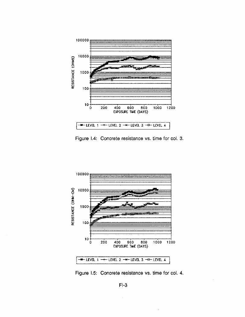
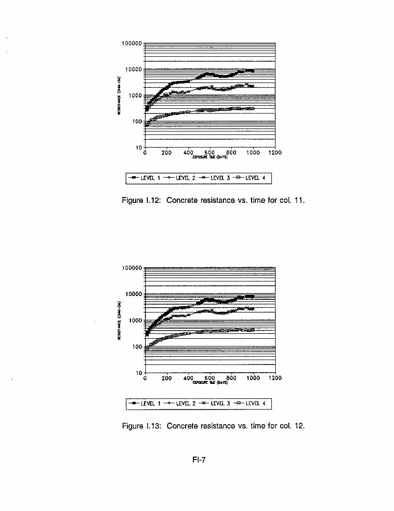
varied with time in all column groups. Figures 1.2 to 1.13 show the evolution of the
interelement resistance of each column through the nearly 3-year test period reported
here. Conversion to nominal concrete resistivity values can be made using the
appropriate cell constant and Eq. (1.1 ). The conversion does not apply for level 3
because resistivity was highly non-uniform at that level, and because the adjacent low
resistance at level 4 provided an additional low resistance current path.
The initial concrete resistances at column level 4 (submerged portion) were
approximately 230Q (about 20,000 Q-cm) for the column group 1 (F+S concrete,
12

Table 1.1 ). The initial resistance was nearly 80 0 (about 7,000 0-cm) for groups 2 to
4 (F concrete). Because of the faster microsilica reaction, the concrete with
microsilica and fly ash should develop lower porosity at early ages compared to the
concrete with fly ash alone [1.3-1.5]. For the same reason, the pore solution pH of the
F+S concrete at early ages should be lower than that of the F concrete. A lower pore
solution pH is also expected to result in higher resistivity of the pore solution [1.6].
Consequently, the observed difference between the early concrete resistivities of types
F+S and Fare in agreement with the expected smaller pore volume and the higher
pore solution resistivity of the F+S concrete. Considering that the concrete was near
water saturation, the absolute resistivity values can be used to obtain a rough
indication of the corresponding Coulomb result that would have been obtained with a
rapid chloride permeability test at the same age. Using the correlation reported in
Reference [1.5], the approximate Coulomb values would have been 800 C for the F+S
concrete and 3,000 C for the F concrete. Those values were in the range of values
expected for the concrete mix designs used [1.5].
The resistance of the submerged portion of the columns increased with time
reflecting the curing process. The resistance was initially smaller in the F concrete
specimens than in the F+S specimens (following the behavior discussed above).
However, the F specimens experienced larger proportional resistance increases with
time than the F+S specimens, so that both types reached comparable resistance
values near the end of the test period. As expected, these trends suggest that in this
permanently wet concrete, the pozzolanic reaction of the fly ash eventually developed
to an appreciable extent (although the reaction of the fly ash was slower than the
reaction of the microsilica). The effect of the microsilica, which strongly differentiated
the resistivity behavior at early ages, was no longer predominant after the system
evolved beyond 2 years. Because the resistance measured at level 4 was
considerably influenced by the resistivity of the concrete between the bars and the
surrounding salt water, the measurements might reflect the effect of chloride intrusion
(as well as some extent of concrete leaching with salt water invasion of concrete
13

pores near the surface) in that region. These are possible causes for the slight
downturn in the resistance at level 4 observed in some of the specimens near the end
of the test period. Disregarding these and other complicating factors, the concrete
resistivity values of both types of concrete (after 3 years of submersion) were in the
30,000 to 40,000 Q-cm range, corresponding to an estimated Coulomb value of about
300 C. That value approaches the range of values reported for similar concrete
mixtures under comparable conditions.
The resistance at the upper levels above water increased with time reflecting a
combination of continuing curing and loss of water by evaporation. The increasing
trend was monotonic during the first year, and showed fluctuations afterwards
reflecting changes in humidity of the surrounding air (all columns) plus the effect of
fresh water surface wetting (columns 6 and 9 since day 230, column 12 during days
230-500 and since day 920, and column 3 since day 920).
The resistivity of the upper concrete in the columns of group 2 (Base, F
concrete) that were not subject to surface wetting approached 600 KO-cm after 3
years. This observation reflected extensive drying of the concrete although a canopy
for increasing water retention was placed at day 666. Resistivity values this high are
not uncommon in concrete exposed for long times to average relative humidities on
the order of 60% to 70%, as present in the laboratory. The resistivity of the upper
concrete in the columns of groups 3 (Silane) and 4 (Siloxane) that were not exposed
to surface wetting followed essentially the same trend as those in Group 2. Thus, the
surface treatments did not alter the drying/curing trends of the concrete under those
conditions. The resistivity of the upper concrete in the columns of group 1 (F+S
concrete) that were not exposed to surface wetting also increased with time.
However, the increase was proportionally less than for the type F concrete columns so
that the concrete resistivity values were eventually similar for both types of concrete.
This behavior is in line with that of the submerged region, suggesting that the
differences between both types of concrete became less marked as the fly ash
undergoes sufficient reaction.
14

Surface wetting of the concrete of the Base group (Column 6) resulted in a
resistivity of the upper level concrete that was two to three times lower than in the
unwetted surface columns in the same group. However, concurrent surface wetting in
the Silane (Column 9) and Siloxane (Column 12) groups during the period 230 to 500
days resulted in no discernible effect. These results suggest that both surface
treatments succeeded in preventing significant ingress of water when it was
periodically sprinkled on the surface of the concrete. As shown above, the treatments
did not cause water to be retained in the concrete. Both observations indicate
desirable results of the treatments, since in an actual field application preventing sea
water entry in the splash-evaporation zone would also hinder chloride ion ingress, and
facilitating concrete drying could reduce the extent of corrosion macrocell activity [1.2,
1.7, 1.8]. Because the resistivity of nearly dry concrete is highly sensitive to relative
humidity changes, the resistivity data showed increasingly higher fluctuations as the
test progressed. Therefore, little information could be derived from the resistivity
monitoring during the last year of the test. The possible effects of wetting column No.
3 (F+ S group) could not be determined.
3.2.2 Steel Potential and Macrocell Current.
Figure 1.14 illustrates the typical potential vs time trends observed for the
various elements within the test columns. Most columns displayed qualitatively similar
behavior. The potential changes with time were generally larger at element 4, in the
portion of the column below water. Figure 1.15 illustrates the typical trends observed
in the test columns for the absolute magnitude of macrocell current flowing between
the various levels. In the long term, the amount of current flowing at switch 3 between
rebar levels 3 and 4 Oust above and below the water line, respectively) greatly
exceeded the amount of current flowing through switches 1 and 2 (in the drier portion
of the columns). This indicated that with the test conditions used in these
experiments, most of the long-term macrocell action was confined between the lowest
two column elements. Therefore, the analysis below will focus on those two elements.
Part II (Section 4) of this report deals with another test system where macrocell action
affecting multiple elements was achieved.
15

Figures 1.16 through 1.19 show the electrode potential of the steel in the
submerged portion of each column group as a function of exposure time. Figures 1.20
through 1.23 show the macrocell current measured at switch 3 (between the
submerged portion and the rest of the column) for each column group as a function of
time.
Shortly after starting the test, all steel elements developed very negative
potentials (as low as -1.1 V SCE in the Microsilica group and -1 V SCE in the Base
group). In the Microsilica group the potentials rose to values of about -250 mV to 0
mV SCE over periods from 100 to 400 days. This was followed by a decrease to
potentials of -300 mV to -500 mV SCE afterwards. Disregarding the first few weeks of
testing, the period of potential rise was associated with the presence of generally
decreasing macrocell currents in which the portion below water behaved as a net
anode. With the exception of element A in column 3, the macrocell currents decayed
from values of 50 ~A to 150 ~A to nearly zero during the potential increase regime.
The later return to more negative potentials was associated with corresponding
increases in the macrocell current of the elements experiencing the potential transition.
The potential in element A of column 3 decayed earlier than any other element, and
the corresponding current started to increase before it had a chance to approach zero.
The Base, Silane, and Siloxane groups experienced potential and current trends
comparable to those of the Microsilica group, except that the initial potential rise to
more noble values took place at a rate that was 2 to 3 times faster than that of the
Microsilica group.
The potential-current trends of the steel in all the test columns may be
interpreted in the idealized manner summarized in Figure 1.24. The analysis assumes
(for simplification) that the portion of the reinforcing steel above water was the site of
only cathodic reactions, while the steel below water was experiencing primarily anodic
16

behavior. Because the steel was placed in the concrete in a strongly pre-rusted
condition with some residual salt contamination, the steel showed highly negative
initial potentials. This is characteristic of steel in the active condition. The steel below
water was likely to quickly consume its immediately surrounding oxygen by means of
cathodic oxygen reduction reactions. Since the oxygen supply through fully
submerged concrete is slow (see Part II), the steel was then expected to have
developed potentials approaching those of the Fe/Fe++ equilibrium. Some deviation
from that equilibrium in the positive direction would be provided by an electronic
macrocell current to the steel portion above water, where oxygen flow across the
partially dry concrete cover should be more efficient. The electronic macrocell current
had the initial value IM1• The current decreased with time as the surface of the steel
below water began to passivate under the action of the alkaline concrete pore solution
environment. This initial period of decreasing macrocell currents is defined in Figure
1.24 as the passivation period. (Macrocell currents during the very first few days of
exposure might in some cases have followed more complicated patterns not
addressed here). After a time, tP , the macrocell current reached very small values
and the steel potential exceeded a value, EPP , which is typically associated with the
condition of steel passivity (as for example in the criterion set by ASTM C-876).
The analysis in Figure 1.24 assumes that (concurrent with the initial passivation
process) chloride ions from the surrounding saltwater had been penetrating the
concrete cover. As a result, the chloride ion concentration at the surface of the
reinforcing steel steadily increased. After a time ti, the concentration exceeded, at
some spot on the steel surface, the amount needed to cause breakdown of the
passive layer. The steel surface on the affected spot became locally active, releasing
iron ions into the surrounding environment and freeing electrons into the steel body.
That event was manifested by a sharp reduction in the steel potential, often followed
by a gentler potential decline as a larger fraction of the steel surface became active
because of increasing chloride contamination and other factors [1.9]. Many of the
17

electrons released by the anodic reactions were consumed in the region above water
by oxygen reduction reactions. This resulted in the development of a sizable
macrocell current that started also at time ti . A smaller fraction of the electrons might
have been consumed below water, depending on the extent of oxygen transport that
the wet concrete would have allowed (see Sections II and Ill). As most of the steel
surface subject to chloride ingress became active, the system approached a steady
state regime characterized by a steel potential EA and a macrocell current 1M2 •
The potential and macrocell current data showed few indications of active
behavior in the segments above the waterline during the test period reported here. In
most cases, as exemplified in Figure 1.14, after the initial passivation stage the
potential of the segments above water remained in the regime usually associated with
passive steel in concrete exposed to air. Figures 1.25 and 1.26 illustrate typical
potential-current behavior for the rebar elements immediately above and below the
waterline. The figures were prepared by plotting the value of the net current of any
given rebar element, as a function of the potential of the same element, for every test
date. The resulting composite diagram shows the overall E-log i record of each
element over 3 years of testing.
For the element below water (level 4), the main cluster of points (around -500
mV and 100 1-1A) corresponds to the active steel behavior encountered during the
earliest and latest stages of evolution. Points at higher potentials and lower currents
correspond to the transition stages at intermediate times. For the element above
water, the main data cluster also corresponds generally to the active stage of the
element below water. The current densities are of the same magnitude as those of
the level 4; but correspond to net cathodic instead of net anodic currents. The overall
data for the cathodic behavior could be approximated by a straight line with slope
between 100 mV and 200 mV per decade. This corresponds to the Tafel slope of the
oxygen reduction reaction [1.2]. The anodic potential-current data could be
approximated by a similar slope only at small current values, but the slope becomes
18

much larger at high currents. This was to be expected if the reaction below water was
predominantly the anodic oxidation reaction, limited by both the extent of the cathodic
reaction above water and the ohmic drop in the concrete between the steel that was
above and below the water.
Only two instances of long-term potentials clearly approaching the active regime
(more negative than -300 mV SCE) were recorded for rebar segments at level 3 of
any column during the test period. These were in columns 10, side A, and column 11,
side A (both in group 4, siloxane ). Near the end of the three-year test period, external
evidence of corrosion above water was observable in the form of a rust spot near the
bottom of level 3 on side A of column 10, a rust spot near the bottom of level 3 on
side A of column 4 (group 2, base), and a fine crack with no rust near the center
elevation of level 3 on side B, also in column 4.
Attempts to evaluate the relative extent of corrosion taking place at elements 4
and 3 were made by means of polarization resistance (PR) and EIS measurements.
These types of measurements detect corrosion only indirectly through the combined
effects of both anodic and cathodic activity, and are subject to many sources of error
[1.10]. Results of EIS tests and polarization resistance measurements performed
during the second year of exposure are provided in Ref.[l.11 ]. The EIS measurements
revealed that the electrochemical response in the columns (both in EIS and PR tests)
was severely complicated by the column geometry and interfacial charge storage
effects. Keeping those limitations in mind, the results of the PR measurements
performed at that time suggested that the level of electrochemical activity was
comparable for all four column groups, and comparable for rebar levels 3 and 4
(immediately above and below the waterline respectively). This was in agreement with
the indications of the potential/current measurements: that the zone above the water
was in most cases not experiencing active corrosion and it was the site of
predominantly cathodic reaction.
19

The evidence discussed above suggests that, during the 3-year test interval,
the zone below water reached an active surface condition quite early (roughly at day
300 for the group with F+S concrete and at day 150 for the groups with F concrete).
A rough estimate can be made of the absolute value of the time that would have been
required for the steel to reach active behavior if simple diffusion mechanisms were
taking place. The resistivity estimates suggested effective chloride diffusion
coefficients of about 0.15 in2 /y [0.97 cm2 /y] and 0.45 in2 /y [2.9 cm2 /y] for the
Microsilica and Base groups respectively [1.5]. (It should be emphisized that
correlations between chloride diffusivity and electric conductivity of the concrete are
only approximate and still subject to controversy [1.13]). For the zone below water,
assuming that the concrete had about 20% average porosity (taking into account the
high water to cement ratio and porous limestone aggregate) saturated with 5% NaCI
water, the region near the surface of the concrete could be expected to acquire a
chloride content approaching 10 pcy [8 Kg/m3]. A chloride concentration threshold for
active corrosion initiation of 1.2 pcy {0.7 Kg/m3) may be assumed on first
approximation [1.5, 1.12]. Nominal application of Fickian diffusion assumptions [1.5,
1.12] and consideration of corner effects [1.5, 1.14] project times to active corrosion
initiation of about 500 and 170 days for the F+S and F concrete groups respectively.
The actual times for the observation of active conditions were comparable to those
projected from the simplified conditions just assumed.
It must be kept in mind that the above analysis used rough approximations .
. Therefore, it is not suitable for a precise evaluation of times to activation of the steel
surface. Chloride transport processes, other than simple diffusion, cannot be
disregarded. Possible acceleration of the corrosion initiation period could result from
additional transport mechanisms for the chloride ions to the rebar surface (convective
processes such as capillary absorption of saltwater shortly following immersion of the
columns, microcracks in the concrete, chloride-flow bypasses through large aggregate
particles, and faster-than-expected chloride transport while the concrete was
undergoing early curing). The slow passivation of the steel (and possible small values
20

of the pore solution pH) might also result in an effective lowering of the chloride
concentration threshold during the early life of the system. Consequently, a reduction
could take place in the time needed for buildup of the necessary chloride content for
depassivation. The data from element A in column 3 (early onset of the chloride
induced stage of corrosion before the initial passivation stage had finished) may
correspond to an example of such behavior.
The evidence to date indicates that severe corrosion had developed in only a
few of the above-water segments (all in columns with concrete F) by the end of the
3-year test period. This finding (subject to confirmation by future monitoring of the
column set) suggests that the chloride concentration threshold for initiation of active
corrosion had not been reached in most of the type F concrete groups or in any of
the F + S column groups that were above water after 3 years of the salting procedure.
This circumstance could have resulted from various possible factors. These include a
higher chloride threshold for the steel in the concrete above water, a slower transport
of chloride through the dryer concrete, or a combination of the above. In addition,
relatively low chloride concentrations on the concrete above water can result because
the salt accumulation mechanism may require some time to develop [1.15, I. 16]. In the
case of the Silane and Siloxane groups, the coatings might have been effective in
reducing chloride accumulation. Exposure and testing of the column groups, including
determination of chloride concentration profiles, will continue in the future to test those
possibilities as mature corrosion patterns develop.
An alternative explanation for the apparently small incidence of corrosion above
water is that the portion of steel below water was acting as a sacrificial anode. If only
segment No.3 (steel area -220 cm2 (0.23 ft2 )) was susceptible to corrosion, the
typical electronic macrocell current ( -100 p.A) sinking into that element in most
columns corresponded then to a protective current density of 0.45p.Ajcm2 {0.43
mA/ft2 ). That amount of protective current approaches values commonly used in
impressed current systems to considerably retard the effect of corrosion [I. 17].
21

The results supported the expectation that the concrete with the higher amount
of pozzolanic replacement, including both fly ash and microsilica, would have the
lowest early permeability and consequently would retard the initiation of corrosion
under the accelerated conditions used. On the other hand, the observed longer time
for steel passivation in the F + S concrete underscored the importance of keeping in
mind the possibly greater susceptibility for corrosion of the steel if the use of
pozzolanic additions results in a significant lowering of the pore solution pH.
In the mode of corrosion operating by the end of the test period (most
corrosion below water), the extent of macrocell current flowing in the F + S concrete
group was not significantly different from that in any of the other column groups. As
suggested by the resistivity results, this is not surprising since (after about two years)
both types of concrete had comparable resistivity values, indicative of similar ohmic
macrocelllimiting effects (see Part Ill) and comparable permeability. As indicated
before, the differences between both types of concrete were expected to become less
as more of the fly ash reacted, a process that appeared to have taken place to a large
extent by the end of the second year. In actual field conditions, with larger concrete
covers over the rebar, the behavior of both types of concrete might be comparable
also from the point of view of chloride ion penetration since most of the transport
would take place after the fly ash reactions reached a mature stage.
The surface coatings succeeded in reducing water entry (and did not increase
retention) in the upper portion of the columns. Those are desirable trends. However,
within the time frame of the experiment, there was no discernible effect on the extent
of macrocell current or in the tendency for corrosion development. Prolonged
monitoring and coring of the columns for chloride profile evaluation will be necessary
to reveal any possible effects.
22

3.3 PART I REFERENCES
1.1. Bennet, J., and Mitchell, T., "Reference Electrodes for Use with Reinforced Concrete Structures", Paper No. 191, Corrosion/92, National Assoc. of Corrosion Engineers, Houston, 1992.
1.2. SagOes, A., Electrochemical Impedance of Corrosion Macrocells on Reinforcing Steel in Concrete, Paper No. 132, Corrosion/90, Nat. Assoc. of Corr. Engs., Houston, 1990.
1.3. Hussain, E. and Rasheeduzzafar, J., Materials in Civil Engineering, Vol. 5, p. 155, 1993.
1.4. ACI Commitee 226, "Silica Fume in Concrete", ACI Materials Journal, Vol. 84, p.158, 1987.
1.5 Berke, N.S. and Hicks, M.C., "Estimating the Ufe Cycle of Reinforced Concrete Decks and Marine Piles Using Laboratory Diffusion and Corrosion Data", p. 207 in "Corrosion Forms and Control for Infrastructure", ASTM STP 1137, Victor Chacker, Ed., American Society for Testing and Materials, Philadelphia, 1992.
1.6 Goni, S., Moragues, A. and Andrade, M.C., "Influence of the Conductivity and the Ionic Strength of Synthetic Solutions Which Simulate the Aqueous Phase of Concrete in the Corrosion Process", Materiales de Construccion, Vol. 39, p. 19, 1989.
1.7 Andrade, C., Maribona, 1., Feliu, S., Gonzalez, J., and Feliu Jr., S., Corrosion Science, Vol. 33, p. 237, 1992.
1.8. Gonzalez, J., Lopez, W. and Rodriguez, P., Corrosion, Vol. 49, p. 1004.
1.9 Aguilar, A., SagOes, A. and Powers, R., Corrosion Measurements of Reinforcing Steel in Partially Submerged Concrete Slabs, p. 66 in Corrosion Rates of Steel in Concrete, N. Berke, V. Chaker and D. Whiting, Eds., STP 1065, ASTM, Philadelphia, 1990.
1.10 SagOes, A. "Corrosion Measurement Techniques for Steel in Concrete", Paper No. 353, 22 pp., Corrosion/93, National Assoc. of Corrosion Engineers, Houston, 1993.
1.11 Hierholzer, S., ''The Effects of Silica Fume and Silicone Concrete Surface Treatments on Controlling Corrosion in Reinforced Concrete Bridge Pilings", M.S. Thesis, University of South Florida, Tampa, November, 1992.
23

1.12 Sagues, A., "Corrosion of Epoxy-Coated Rebar in Florida Bridges", Final Report to Florida D.O.T., WPI No. 0510603, University of South Florida, Tampa, May, 1994.
1.13 Pfeifer, D., McDonald, D.B. and Krauss, P., PCI Journal, p.38, JanuaryFebruary, 1994.
1.14 Sagues, A., Research in Progress, 1994.
1.15 K.Uji, Y.Matsuoka and T.Maruya, "Formulation of and Equation for Surface Chloride Content of Concrete Due to Permeation of Chloride", in Corrosion of Reinforcement in Concrete, C.Page, K.Treadaway and P. Bamforth, Eds., p.258, Elsevier, New York, 1990.
1.16 Bamforth, P.B., "Concrete Classifications For R.C. Structures Exposed to Marine and Other Salt-Laden Environments", 11 pp., Paper presented at "Structural Faults and Repair", Edinburgh, June 29-July 1, 1993.
1.17 J.Bennett, J. Bartholomew and T. Turk, "Cathodic Protection Criteria Related Studies Under SHRP Contract", Paper No. 323, Corrosion/93, NACE International, Houston, Texas, 1993.
24

COLUMN GROUP
1 (MICROSILICA)
2 (BASE)
3 (SILANE)
4 (SILOXANE)
TABLE 1.1 COLUMN GROUPS
COLUMN CONCRETE No.
1-3 F+S
4-6 F
7-9 F
10-12 F
25
SURFACE TREATMENT
NONE
NONE
SILANE
SILOXANE

NC SWITCHES
TO BOX
ELEMENT.#
1
2
3
4 f
INTERNAL REFERENCE ELECTRODE
WATER LINE
Figure 1.1 Column ~iring Schematics.
Fl-1

100000
,..... 10000 Vl :I ::t 0 '-" w
1000 l..l z <(
i _ ....
E ·~
1-Vl iii
iSP"
w 100 a::
10 0 200 400 600 800 1 000 1200
EXPOSl.m: TIME (DAYS)
1--LEVEL 1 -+- LEVEL 2 """'*-- LEVEL 3 -a- LEVEL 4
Figure 1.2: Concrete resistance vs. time for col. 1.
100000
- 10000 ----1/) ::E :X: 0 '-" w
1000 (,) z .( ~- ~
1-Vl iii l!llP" w a:: 100
10 0 200 400 600 800 1000 1200
EXPOS~E TIME (DAYS)
1-- LEVEL 1 --- LEVEL 2 _,__ LEVEL 3 -e- LEVEL 4
Figure 1.3: Concrete resistance vs. time for col. 2.
Fl-2
100000
- 10000 1/l ::f I 0 -11.1
1000 u z < ~
_.,
.... !a 1/l --11.1 « 100
10 0 200 400 600 800 1000 1200
EXPOSLFE TIME (DAYS)
1-- LEVEL 1 -+- LEVEL 2 __._ LEVEL 3 -s- LEVEL 4
Figure 1.4: Concrete resistance vs. time for col. 3.
100000
- 10000 ::f y
..... ~
::f
~ .....,. 11.1 1000 u z < .... !a 1/l 11.1 100 «
~ ~ "'""""'*'" ..... """'
-""
10 0 200 400 600 800 1000 1200
EXPOSI.FE TIME (DAYS)
1-- LEVEL 1 -+- LEVEL 2 __._ LEVEL 3 -s- LEVEL 4
Figure 1.5: Concrete resistance vs. time for col. 4.
Fl-3

,....._ JE y JE :I: 0 ......, w 0 z -4: 1-!l1 VI w 0::
-::::E y ::::E
~ -w u z 4 1-VI iii w 0::
100000
10000
1000
100
10
li5!!l ,;.e- ~ ~"T
F
"diJIP'
0 200 400 600 800 1000 1200 EXPOS~E TIME (DAYS)
1-- LEVa 1 -+- LEVEL 2 ...._ LEVa 3 -e- LEVEL 4
Figure 1.6: Concrete resistance vs. time for col. 5.
100000
10000
1000 rr-~~ ,._.,
"' 100
_,
10 0 200 400 600 800 1000 1200
EXPOS~E TIME (DAYS)
1-- LEVEL 1 -+-- LEVEL 2 ...._ LEVEL 3 -e- LEVEL 4
Figure I. 7: Concrete resistance vs. time for col. 6.
Fl-4

100000
10000
I I 1000
100
J/111'"' _,.~
.._. .,.,......
""' ~
10 0 200 400 600 800 1000 1200
ElO'OSIJI£ lW: (.IMYS)
1--LEVEL 1 -- LEVEL 2 -- LEVEL 3 -e- LEVEL 4
Figure 1.8: Concrete resistance vs. time for col. 7.
100000
10000
I I 1000
100
~ ~-
. ._.
z 10
0 200 400 600 800 1 000 1200 ElO'OSIJI£ lW: ()I.I.YS)
1-- LEVEL 1 -- LEVEL 2 -- LEVEL 3 -e- LEVEL 4
Figure 1.9: Concrete resistance vs. time for col. 8.
Fl-5

100000
10000
_.., .......... l I 1000 1' ,
~ 100
10 0 200 400 600 800 1000 1200
EXPOSIJIE 1W: (.bAYS}
1-- LEVEL 1 -+- LEVEL 2 -*-- LEVEL 3 -e- LEVEL 4
Figure 1.1 0: Concrete resistance vs. time for col. 9.
100000
10000
""" ...-: ........ ~ l ~ 1000 • ~
100 ~
10 0 200 400 600 800 1000 1200
EXPOSIJIE 1W: (.riA YS}
1-- LEVEL 1 -+- LEVEL 2 ---- LEVEL 3 -e- LEVEL 4
Figure 1.11: Concrete resistance vs. time for col. 10.
Fl-6
100000
10000
..... '"" ill""""'"·""'·----
~
I I 1000
I I
100
10 0 200 400 600 800 1000 1200
EXPOSI.R£ TU: (ll.t. YS}
1-- LEVEL 1 -+- LEVEL 2 ~ LEVEL 3 -e- lEVEl 4
Figure 1.12: Concrete resistance vs. time for col. 11.
100000
10000
__... .~.
1000 ~- -I""
100 ~
10 0 200 400 600 800 1000 1200
EXPOSI.R£ TU: (ll.t. YS}
1-- LEVEL 1 -+- LEVEL 2 ~ lEVEl 3 -e- lEVEl 4
Figure I. 13: Concrete resistance vs. time for col. 12.
Fl-7

....-. > E .........
,..-... w 0 (/)
(/)
> a: <C Ill .......... -I <C 1-z w 1-0 c._
POTENTIAL VS. TIME (COL 1) 0
-100
-200
-300
-400
-500
-600
-700
-800
-900
-1000 0 100 200 300 400 500 600 700 800
TIME (DAYS)
j-s- LEVEL 1 A -t- LEVEL 2A ~ LEVEL 3A ---.;..- LEVEL 4A
Figure 1.14 Potential vs. Time Trends for Rebar On Side A of Column No. 1 (S +F Concrete).
Fl-8
900

1-z w a: a: ::::,)
0
COL3 SARA
0.1 = D
0.01WR~----~------r----4~-E~~~ffi8&-.-------.-----~
0 200 400 600 800 1 000 1200 TIME (DAYS)
~
o SWITCH lA + SWITCH 2A * SWITCH 3A
Figure 1.15 Example of Magnitudes of the Macrocell Currents Flowing Through Switches {Switch No. 1 is the Highest) as a Function of Time. {Side A, Column No. 3, S + F concrete)
Fl-9

~ LLJ 0 (/)
~ LLJ
~ LLJ 0 (/)
~ LLJ
0
-200
-400
-600
-800
-1000 0
* 0
-200
-400
-600
-800
-1000
200
COL1
COVERED WIT~ POL YTHENE SHEET
:coL 3 SUBJECTE : TO MOISTENING
SIDE A
400 600 686 800 920 1 000 1200
0
EXPOSURE TIME (DAYS)
COL2 0 COL3
COVERED WITH POL YTHENE SHEET
:coL 3 SUBJECTED !TO MOISTENING
SIDES
600 686 800 920 1 000 1200
EXPOSURE TIME (DAYS)
* COL 1 0 COL2 0 COL3
Figure 1.16 Open Circuit Potential vs. Time at Level 4 in Group 1.
Fl-10

0
-200
l -400
w () SIDE A 0 <J) -600 > w
-800
-1000 0 200 400 600 666 800 1000 1200
EXPOSURE TIME (DAYS)
* COL4 0 COL5 D COL6
0
-200
-400
l w ()
SIDEB 0 -600
~ w
-800
-1000 0 200 400 600 666 800 1000 1200
EXPOSURE TIME (DAYS)
* COL4 0 COL5 0 COL6
Figure 1.17 Open Circuit Potential vs. Time at Level 4 in Group 2.
Fl-11

0
-200
~ -400 w 0 (/)
SIDE A ~ UJ -600
-800
-1000 0 200 400 600 666 800 1000 1200
EXPOSURE TIME (DAYS)
* COL7 0 COL8 0 COL9
0
-200
~ -400
w SIDEB 0 (/)
~ -600 UJ
-800
-1000 0 200 400 600 666 800 1000 1200
EXPOSURE TIME (DAYS)
* COL7 0 COL8 0 COL9
Figure !.18 Open Circuit Potential vs. Time at Level 4 in Group 3.
FI-12

0
-200
=e -400
(jJ SIDE A 0
0
~ -600
I.IJ
-800
-1000 0 200 400 600 666 800 1000 1200
EXPOSURE TIME (DAYS)
* COL 10 0 COL 11 D COL 12
0
-200
=e -400 (jJ SIDES 0 0
~ -600 I.IJ
-800
-1000 0 200 400 600 666 800 1000 1200
EXPOSURE TIME (DAYS)
* COL10 0 COL11 0 COL12
Figure !.19 Open Circuit Potential vs. Time at Level 4 in Group 4.
FI-13

l !z w a: a: :::> 0 ::l U.J 0 0 a:
~
200
-200
0 200
200
100
0
-100
-200
0 200
400
COVERED WITH
~COL 3 SUBJECTED
!TO MOISTENING
600 686 800 920 1000 1200
EXPOSURE TIME (DAYS)
* COL 1 0 COL2 0 COL3
fCOVERED WITH f ' '
POL YTHENE SH~ET
:coL 3 SUBJECTE
TO MOISTENING
SIDE A
SIDEB
400 600 686 800 920 1 000 1200
EXPOSURE TIME (DAYS)
* COL 1 0 COL2 0 COL3
Figure !.20 Macrocell Current vs. Time at Switch 3 in Group 1.
FI-14

200
1 100
!z LU a:
SIDE A a: 0 ::> ()
::1 LU () 0 -100 a:
i -200
0 200 400 600 666 800 1000 1200
EXPOSURE TIME (DAYS)
* COL4 0 COL5 0 COL6
200
1 100
!z LU a:
SIDE 8 !5 0 ()
::1 LU () 0 -100 a:
i -200
0 200 400 600 666 800 1000 1200
EXPOSURE TIME (DAYS)
* COL4 0 COL5 0 COL6
Figure 1.21 Macrocell Current vs. Time at Switch 3 in Group 2.
FI-15

200
100
1 ~
0 SIDE A
UJ a: a: ::::> () -100
-200
0 200 400 600 666 800 1000 1200
EXPOSURE TIME (DAYS)
* COL7 0 COL8 0 COL9
200
100
< SIDES 0 .a. ~ UJ a: a: ::::> -100 ()
-200
0 200 400 600 666 800 1000 1200
EXPOSURE TIME (DAYS)
* COL7 0 COL8 0 COL9
Figure I.22 Macrocell Current vs. Time at Switch 3 in Group 3.
FI-16

200
100
1 0
~ w ~ :J -100 (.)
-200
200
100
1 0
~ w a: a: :J -100 (.)
-200
0 200
0 200
400 600 666 800 1000
EXPOSURE TIME (DAYS)
* COL 1 0 0 COL 11 0 COL 12
400 600 666 800 1000
EXPOSURE TIME (DAYS)
* COL 7 0 COL8 0 COL9
Figure 1.23 Macrocell Current vs. Time at Switch 3 in Group 4.
FI-17
SIDE A
1200
SIDES
1200

POTENTIAL
Ep ------------------=-~-~-~-.---~
Epp --------I
I I I I
----+---------------1-----~-~-------------1 I I I \ \ I I I I I I I I I I I I I
I
I I
CURRENT I I I I
1!.11 : I I I I I
TIME
I I I M2 - -------1------------- --+- -------------:--=-------------
1 I I I I I I I I I I I I I I I I I
tp tl TIME - - ACTIVE STAGE -7/- .... - -
PASSIVATIO"' PASSIVE
PERIOD PERIOD
INITIATION - PROPOGATION -7/- ... -
Figure I.24 Interpretation of Potential and Current Trends.
FI-18

> E -w (.) en ~ w
0
-1
-200
-4oo••
-500
-600
-700
-800
COL1 LEV4A-NETCURRENT
• II • ·n -,_ ,. I u • •• ~ -~
I I II
II II -++ I
tffl 1111+
-1
Ill I ~rt!ill Ill 000 I I
0.01 0.1 1 10 100 CURRENT NET (uA)
Figure !.25 Example of Potential-Net Current Composite Polarization Behavior for the Rebar Element Below the Waterline (Element No. 4, Side A, Column 1, S +F).
FI-19
1000

> E -w 0 (/)
C/)
> w
0
-100
-200 ,
-300
-400
-500
-600
-700
-800
-900
-1000 0.01
COL 1 LEV 3A - NET CURRENT
* ~ l±U '-'~f;;;;FE
* ;;>!*
*
*
tl w ~ I 0.1 1 10 100 1000
CURRENT NET (uA)
Figure I.26 Example of Potential-Net Current Composite Polarization Behavior for the Rebar Element Immediately Above the Waterline (Element No. 3, Side A, Column 1, S + F).
FI-20

4. PART II: EFFECT OF CONCRETE MOISTURE.
4.1 PROCEDURE
4.1.1 Concrete Columns.
Instrumented reinforced concrete columns identical to those of a previous work
[2.1] were used in this investigation. The columns were designed to simulate a slice
from an actual pile, where the exterior portion is dryer than the interior portion. The
columns were constructed with a base configuration of 12 by 4 by 46 in (30.5 by 10.2
by 122 em) and with an inset of 0.5 in (1.3 em) on one side. Eleven segments of #7
(2.2 em nominal diameter) regular •black• rebars were placed horizontally at 4 in (10.2
em) center-to-center spacing. The length of each rebar segment was 9 in (22.9 em).
The bars were placed slightly off-center facing the inset to allow for reduced concrete
cover on one side. The intention was to simulate the cross-sectional moisture
gradient that normally is encountered in a pile. The rebar segments were numbered
from No.1 (at the top of the column) to No. 11 (at the bottom). Figure 2.1 depicts the
main features of the test columns.
Each rebar had an activated titanium reference electrode placed about 0.5 in
(1.3 em) below the bottom. Electrical connections were made to all rebars and
associated reference electrodes. All rebars were normally interconnected by toggle
switches. The switches were numbered from No. 1 (below rebar element No.1) to No.
10 (below rebar element No. 10). The electrical connections to the bars were covered
by metallographic epoxide compound to prevent unwanted galvanic action. The rebar
segments were pre-rusted before concrete placement, in the same manner as the
bars used for the laboratory columns in Part I. Other details on the column
construction can be found in Refs [11.1-11.2].
26

4.1.2 Concrete.
The concrete mix design was the same for all columns. The mix design was
based on a standard FOOT design using Type I Portland cement with a cement factor
of 611 pcy (360 Kg/m3 ), limestone coarse aggregate, and silica sand. A w/c ratio of
0.45 was used. Because a low concrete cover was used in the columns, the coarse
aggregate size (3/8 in; 1 em) was smaller than that normally used in bridges, on
account of the low concrete cover used in the columns. To accelerate the test, the
concrete mix for the lower 10 in (25.4 em) of each column had an addition of 20 pcy
(11.8 Kg/m 3 ) of chloride ion, obtained by using the appropriate amount of NaCI.
Rebar elements No. 10 and No. 11 were in the high chloride zone. Rebar element
No.11 was also just below the waterline (see the next paragraph).
4.1.3 Testing Environment.
A total of 4 columns , labeled A, B, C and D were prepared. The columns were
moist-cured for 5 days after casting, and then exposed to the laboratory air for 6
additional days. All the columns were then put in an exposure tank so that the lower
5 in (12.7 em) were immersed in water containing 5% NaCI solution. The rebar
segments within each column were electrically interconnected shortly afterwards.
Exposure time was counted from the nominal moment of rebar interconnection.
All testing was performed at ambient room temperature (typically 21°C±1°C)
and ambient room relative humidity (typically 60% ± 1 0%). The upper portion of all the
columns was allowed to dry in room temperature and humidity conditions for the first
343 days of exposure. Then the above-water surface of columns A and D was
subjected to controlled applications of fresh water moisture. This was performed by
covering the plain vertical face of each of the two columns with plastic sheets, and
pouring fresh water from the top of the column inside the plastic cover three times a
week. This resulted in permanent water saturation of that face of the column while the
other face (with the inset) remained surface-dry. This condition of columns A and D
will be referred from here on as the •partially wet• condition. Starting at day 681, the
27

wetting procedure was extended to both faces of columns A and D, resulting in water
saturation of the entire column. This condition will be called the .. fully wet .. condition.
Columns Band C, not wetted above the waterline, acted as controls and will be
referred to as the •non-wetted• columns.
4.1.4 Corrosion Monitoring.
During the test exposure, periodic electrochemical measurements were made
on each column. The following parameters were monitored: (1) Static potential
measurements of each rebar segment with respect to the immediately surrounding
concrete, (2) macrocell current flowing through the switches joining the rebar
segments, and (3) resistivity of the concrete at elevations corresponding to the space
between the rebar segments. The procedures for these measurements have been
described in detail in Refs. [11.1-11.2).
4.2 RESULTS AND DISCUSSION
4.2. 1 Concrete Resistivity.
Figures 11.2 to 11.5 show the evolution of the concrete resistivity at various
elevations of each column during the 3-year exposure period. The non-wetted
columns experienced a general increase in resistivity of the upper levels with time,
with fluctuations reflecting variations in room relative humidity. The highest resistivity
levels encountered are comparable with those of the non-wetted columns examined in
Part I of this investigation, and with values usually reported for dry concrete of similar
composition [11.3]. At the lowest levels, the resistivity was nearly constant, while at
intermediate levels, the resistivity reached a maximum after about one year and then
began to decline again. This latter behavior possibly reflects the increasing
contamination with chloride ions shortly above the waterline, which resulted in a
reduction in pore solution resistivity and a better retention of moisture.
28

The resistivity of the wetted columns clearly reflected the effect of wetting.
One-side moistening was enough to create a dramatic reduction on the average
resistivity of the upper column regions. Moistening the entire upper portion of the
column resulted in resistivities throughout the column that were less than 5,000 0-cm,
a value comparable with some of the most severe field conditions encountered in
marine substructures in Florida [11.5]. The resistivity values of these conditions
correspond to Coulomb test values of roughly 4,000 C in the Rapid Chloride
Permeability test. This is consistent with the high w/c ratio and unblended cement
concrete used in these experiments [11.6, 11.7].
4.2.2 Steel Potential and Macrocell Currents.
Figures 11.6 and 11.7 show the steel potential measured at the two lowest
column elevations (where chloride ion contamination was present from the start) as a
function of exposure time and wetting condition. Unlike the case of the columns in
Part I of this report, the steel even in the high chloride region showed potentials
associated with passive behavior at the beginning of the test period. The potential
decayed rapidly toward active values and experienced a further, slow decrease
throughout the experiment. The potential in the high chloride portion of the columns
being wetted (A and D) dropped to the lowest values by the end of the 3-year test
period. Figure 11.8 shows the steel potential as a function of elevation after the
columns had acquired a mature corrosion pattern under the either non-wetted or
partially wet conditions (day 681). The non-wetted columns (B,C) showed a range of
potentials from very active near the bottom to clearly passive behavior at the top. The
partiallly wet columns (A,D) showed also a distribution of potentials but with less of a
difference between the upper and lower regions. Figure 11.9 shows the result of the
same type of measurements after the full-wetting regime had been developed for
columns A and D. The potential profiles for the dry columns Band C remained similar
to those in Figure 11.8; the fully wet columns developed a potential regime that was
more narrow than before.
29

Figures II. 1 0 and 11.11 show the corrosion macrocell current patterns after the
systems matured in the dry, partially wet and fully wet regimes. The plots show the
currents flowing through the switches that interconnected the rebar segments at the
various elevations. The amount of macrocell current actually flowing from or sinking
into a given rebar element is given by the difference between the current passing
through the switches above and below the element. The values of the net currents
were computed for each condition and the results are shown in Figures 11.12 and 11.13.
The electronic macrocell currents were commonly flowing from the lowest to the
highest elevations. This was expected because the chloride contamination around the
lowest elements caused them to behave as anodes while the upper elements tended
to behave as cathodes because of the absence of chloride (and easier oxygen
availability except when very wet). The net current calculations confirmed the net
anodic character of the lowest rebar element (No. 11 ), indicating that electron
generation in that element significantly exceeded its consumption by cathodic
reactions. While element 10 (and possibly 9 later in the exposure life) was also the
site of anodic reactions, its net character was either cathodic or anodic depending on
the relative electron demand on its surface and that of the upper elements for cathodic
reactions. Elements above 9 were invariably net cathodes.
The rate of the cathodic reaction in the upper elements depended on the
electron supply from the corroding elements at the lower levels. The electronic current
was in turn determined by the polarization of the cathodic reaction (both by activation
and concentration mechanisms), the potential of the anodic bars, and the resistive
potential drop due to the intervening concrete between anodic and cathodic regions.
The latter effect was responsible for the gradual drop in cathodic activity with
increasing elevation. Application of moisture reduced the concrete resistivity and
consequently the extent of ohmic potential drop. The effect is manifested in the
increased macrocell current at the upper levels of columns A and D upon partial
wetting and later full wetting (Figures 11.10 to 11.13). Net cathodic currents
experienced dramatic relative increases (on a percent basis) as a result of wetting. To
30

better visualize those increases, the absolute values of the net sink or source currents
at each element are shown in Figures 11.14 to 11.17. These plots illustrate the various
stages in the life of the columns. Full wetting of the columns resulted in net cathodic
current levels at the upper elements that were almost two orders of magnitude greater
than for the unwetted columns.
Although surface wetting reduced the disparity between the amount of cathodic
current among the rebar elements in chloride-free concrete, the effect on overall
corrosion activity of the column was more complicated. Figure 11.18 shows the total
amount of net anodic current measured in the columns. The data for the early stages
of evolution, before column wetting, shows that there is considerable variability from
specimen to specimen. Application of partial wetting to columns A and D resulted in a
significant increase in overall macrocell current in both columns. However, the
increase was no larger than the column-to-column variability illustrated by the
difference in behavior between the dry columns 8 and C. Application of full wetting
caused the overall anodic currents of columns A and D to actually drop from the
values experienced under partial wetting (columns 8 and C continued their previous
behavior).
The varying effect of increasing amounts of moisture on the overall corrosion
intensity can be further examined by plotting the potentials versus cathodic current of
the segments in the chloride-free concrete, in the manner of an E-log i plot. Figure
11.19 shows the composite behavior of all segments in the four columns near the end
of the partial wetting period. The data delineate a polarization curve descriptive of the
oxygen reduction reaction, approaching an activation Tafel slope between 100 mV to
200 mV per decade [11.1] in the low current portion of the curve. At high current
densities there is a suggestion of the onset of concentration polarization. The data
for the unwetted columns span a relatively wide range, showing how the polarization
available at the upper column portions is quite small. The wetted columns achieved
larger cathodic polarization at the upper regions as a result of the lower resistive drop
in the moist concrete. The potential range of the cathodic elements in those columns
was consequently smaller and approached the potential of the anodic regions.
31

The effect of full column wetting is manifested in Figure 11.20. The polarization
behavior in the unwetted columns remained as before. The potentials in the cathodic
portions of the fully wetted columns became even lower than before. However, the
cathodic currents became about the same for all elements and were limited to a
smaller value than in the partially wetted case. The behavior is characteristic of
diffusional limitation. The difference in behavior between the partially and fully wetted
cases can be explained by the dependence of the speed of oxygen transport in
concrete with its moisture content. In the partially wetted case, only one side of the
concrete slab was wetted which reduced the resistivity of the concrete and
consequently the ohmic drop across the macrocell. The opposite side of the slab
remained partially dry, which created relatively little hindrance to oxygen transport
across the concrete cover [11.8]. In the fully wetted case, both sides of the columnar
slab were wetted which resulted in nearly water-saturated concrete. Under those
conditions oxygen transport can become several orders of magnitude slower than in
the partially wet case [11.8]. While the ohmic drop becomes still smaller under those
circumstances, the oxygen supply is much smaller and diffusional limitation of the
cathodic current results. This interpretation is in agreement with the observed drop in
macrocell currents observed upon application of full wetting to columns A and D.
A rough estimate of the effective diffusion coefficient, D, for oxygen in concrete
can be made for the fully wetted case by simplifying the system as an one
dimensional flow case, with a concrete cover h of 1 in (2.5 em), and an approximate
steel/concrete surface ratio of 1:1. Under those conditions the limiting current density
i1 is given by
i1 = 4 F D Cs I h (11.1)
where F is the Faraday constant and Cs is the effective concentration of oxygen at the
concrete surface. Since the rebar segments have a surface area approaching 100
cm2 , then per Figure 26, i1 - 0.3 !J.A/Cm2
• Cs (when expressed in terms of
concentration in the pore water) can be taken to be approximately equal to 3 1 o·7
mol/cm3 if equilibrium between air and fresh water is assumed. Those parameters
32

yield D - 6 1 o·6 cm2 /sec . This value is consistent with measurements reported in
the literature for water-saturated concrete (after appropriate accounting of the manner
in which oxygen concentration is defined} [11.9-11.13] and supports the above
interpretation of the polarization behavior observed.
The results of these experiments confirmed the general expectations of
behavior in substructure conditions, and agreed with the predictions of earlier
theoretical models of macrocell behavior [11.1] as well as with the calculations
presented in Part Ill. A noteworthy finding of this part of the project was that
intermediate amounts of moisture can increase macrocell action significantly by
reducing the extent of resistive polarization. However, when the moisture additions
cause water saturation, the effect of resistance reduction is offset by a decrease in the
oxygen supply.
33

4.3 PART II REFERENCES
11.1 SagOes, A., Perez-Duran, H. and Powers, R., Corrosion, Vol. 47, p. 884, 1991.
11.2. AI-Mansur, A.K.M., "Effect of Moisture Application on the Corrosion Behavior of Reinforcing Steel in Marine Bridge Substructures", M.S. Thesis, University of South Florida, Tampa, Florida, December, 1992.
11.3. Monfore, G., ''The Electrical Resistivity of Concrete", Journal of the PCA Research and Development Laboratories, May 1968, p. 35.
11.4. Millard, S. G., Ghassemi, M., Bungey, J. and Jatar, M., "Assessing the Electrical Resistivity of Concrete Structures for Corrosion Durability Studies", in Corrosion of Reinforcement in Concrete, C. Page, K. Treadaway and P. Bamforth, Eds., p. 303, Elsevier Appl. Sci., London-New York, 1990.
11.5 SagOes, A., "Corrosion of Epoxy-Coated Rebar in Florida Bridges", Final Report to Florida D.O.T., WPI No. 0510603, University of South Florida, Tampa, May, 1994.
11.6 Berke, N.S. and Hicks, M.G., "Estimating the Life Cycle of Reinforced Concrete Decks and Marine Piles Using Laboratory Diffusion and Corrosion Data", p. 207 in "Corrosion Forms and Control for Infrastructure", ASTM STP 1137, Victor Chacker, Ed., American Society for Testing and Materials, Philadelphia, 1992.
11.7 Feldman, R., Chan, G., Brousseau, R. and Tumidajski, P., ACI Materials Journal, Vol. 91, p. 246, 1994.
11.8. Tuutti, K., Corrosion of Steel in Concrete, Swedish Cement and Concrete Research Institute, Stockholm, 1982.
11.9 Page, C. and Lambert, P. J., Mat. Sci., Vol 22, p. 942, 1987.
11.10 Yu, S. and Page, L, Cement and Concrete Research., Vol. 21, p. 581, 1991.
11.11 0. Gjorv, 0. Vennesland and A. EI-Busaidy, Materials Performance, Vol. 25, No. 12, p. 39 (1986).
11.12 Kobayashi, K., Cement and Concrete Rsch., Vol. 21, p. 273, 1991.
11.13 Ohama, Y. and Demura, K., Cement and Concrete Research., Vol. 21, p. 309, 1991.
34

l 48"
l
4.5"
1
T--4"
+--4" J.. __
12"
~ 111 ;·I I I
1----4 1 -·112" INSET
~T I 2 5" D- __ l TOP VIEW
2" 2"
TO CONNECT I ON BJX
FRONT VIEW
ELECTRODE _, ~ ' - - - - -.. / ....
REFERENCE \
'-- __ -- ~ REBI\R SE~ENTS (SIZE #7) 11 SEGMENTS ON 4" CEtfTER
T-- --- I HIGH INITIAL
4" ~TER_L~~E CHLORIDE +-- T iO" ZONE
r __ '-------------' __ L ____ l ___ _
LABORATORY COLUMN CONFIGURATION
Figure II.l Sketch of the Laboratory Column Configuration.
Fil-l

100000
:i 80000
'-? ::::!: MOIST (ONE SIDE) MOIST (ALL SIDES) :r:
60000 Q.
i 40000 (/) LU a:
20000
0 0 200 400 600 800 1000 1200
EXPOSURE TIME (DAYS)
* LEVEL 1 0 o LEVEL 9 o LEVEL 8 .6. LEVEL 1
Figure II.2 Concrete resistivity (Column A).
100000
80000 DRY MOIST (ONE SIDE) MOIST (ALL SIDES) :i 9 ::::!: 60000 :r: Q.
~ 40000
se (/) LU
20000 a:
0 0 200 400 600 800 1000 1200
EXPOSURE TIME (DAYS)
* LEVEL 1 0 o LEVEL 9 o LEVEL 8 A LEVEL 1
Figure II.3 Concrete resistivity (Column D).
FII-2
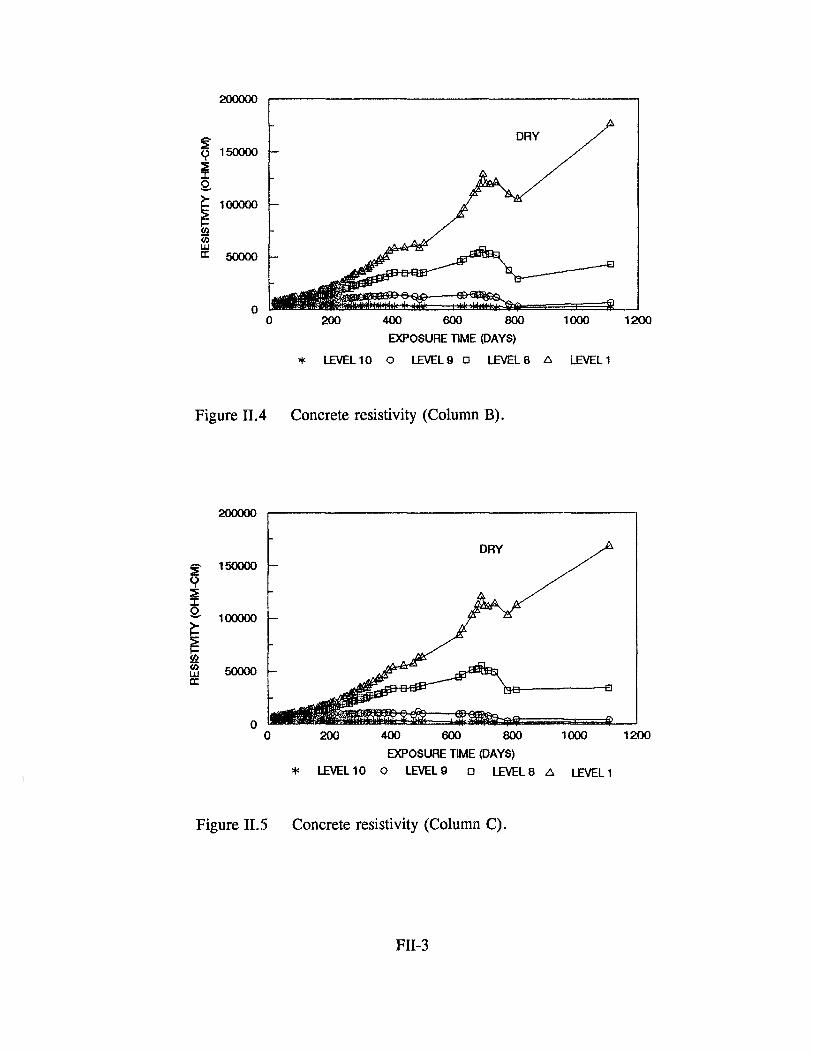
200000
~ 150000
DRY
:::E J: Q.
~ 100000
(/) (i) UJ a: 50000
0 0 200 400 600 800 1000 1200
EXPOSURE TIME (DAYS)
* LEVEL 1 0 o LEVEL 9 o LEVEL 8 t:. LEVEL 1
Figure II.4 Concrete resistivity (Column B).
200000
DRY
~ 150000 <;> :::E J: Q. 100000
~ (i)
50000 UJ a:
200 400 600 800 1 ()()() 1200
EXPOSURE TIME (DAYS)
* LEVEL 10 0 LEVEL 9 o LEVEL 8 1:>. LEVEL 1
Figure II.5 Concrete resistivity (Column C).
FII-3

0
-100 DRY MOIST (ONE SIDE) MOIST (AU.. SIDES)
(jJ -200 0 (/)
~ -300 g L.U -400
-500
-600 0 200 400 600 800 1000 1200
EXPOSURE TIME (DAYS)
* COLA 0 COLB D COLC /::,. COLD
Figure II.6 Static Potential Measured at LevellO.
0
DRY MOIST (ONE SIDE) MOIST (AU.. SIDES)
-100
(jJ 0 -200 (/)
~ > s -300
w
-400
-500
-600 0 200 400 600 800 1000 1200
EXPOSURE TIME (DAYS)
* COLA 0 COLB D COLC /::,. COLD
Figure II. 7 Static Potential Measured at Level 11.
FII-4

48
44
fii 40 w I (.)
36 z
32 :;:::::...
z ~ 28 ::J ....J 0 24 (.)
w 20 I
I-z 16 I-I
12 (!) w I 8
4
0 -1000 -800 -600 -400 -200 0
* COL A 0 COL 8 D COL C 6 COL D
E(mV VS. SCE)
Figure II.8 Static Potential vs. Height (Day 681).
FII-5

fii w I () z ::::;::..
z ~ ::J ...J
8 w I 1-z II C) w I
48
8
4
0 -1000 -800 -600 -400 -200
6. COLD D COLC 0 COLB * E (mV VS. SCE)
Figure II.9 Static Potential vs. Height (Day 1111).
FII-6
0
COLA

-CJ) w I (.)
3 z :;:::::..
z ~ ::J .....1 0 (.)
w I r-z r-I CJ w I
0 0 200 400 600 800 1000
* COLA 0 COLB 0 COLC 6 COLD
MACROCELL CURRENT (uA)
Figure 11.10 Macrocell Current vs. Height (Day 681).
FII-7

fii w I (.) z :::::;::..
z ~
3 0 (.)
w I 1-z II (!) w I
4
4
3
3
0 0
WATER LINE
200 400 600 800
* COL A 0 COL B D COL C D, COL D
MACROCELL CURRENT (uA)
Figure II.11 Macrocell Current vs. Height (Day 1111).
FII-8
1000

ANODIC CATHODIC .......... (f) w I () z ::::::;:..
z ~ ::> _J
0 ()
w I 1-z 1-I c;, w I 8 WATER LINE
4
0 -1000 -500 0 500 1000
* COLA 0 COL B D COL C !:::. COLD
NET CURRENT (uA)
Figure II.12 Net Current vs. Column Height (Day 681).
FII-9

en 4o w I (.) z ::::::... z ~ :J _J
0 (.)
w I ._ z
~ (!) w I
24
20
i6
i2
8
4
O -iOOO
ANODIC CATHODIC
WATER LINE
-500 0 500
NET CURRENT (uA)
* COLA 0 COLB D COLC 6 COLD
Figure 11.13 Net Current vs. Column Height (Day 1111).
FII-10
iOOO

48
...._40 (/)
~ ~ '-" 3 2 ~ ~ u ~24 ;l;; 1-
~16 w I
8
0+---~~~~~--~--~~~~--~~~~~~--~~~~~
0.1 1 10 100 1000 NET ~RENT (uA)
1-- COL A -+- COL B --*-- COL C -E1- COL D
Figure ll.l4 Absolute Value of Net Current vs. Colunm Height (Day 90).
FII-11

48
8
0+---~~~~~--~--~~~~--~~~~~~--~~~~~
0.1 1 10 100 1000 NET ~RENT (uA)
1- COL A -+- COL 8 --*- COL C -E3- COL D
Figure II.l5 Absolute Value of Net Current Associated With Rebar Segments vs. Column Height (Day 300).
Fll-12

48
..... .40 (I) ...... :I: 0 ;.:; '""32 ~ ~ 0
~ 24 .... ;:;;
~16 ~
8
0+---~~~~~--~--~~~~--~~~~~~--~~~~~
0.1 1 10 100 1000 HET <:rnRENT (uA)
1- COL A -+- COL 8 --*-- COL C -a- COL D
Figure II.16 Absolute Value of Net Current Associated with Rebar Segments vs. Column Height (Day 442).
FII-13

48
8
o+---~~~~~--~~~~~~--~~~~~~--~~~~~
0.1 1 10 100 1000 NET ctJ(RENT (uA)
1- COL A -+- COL 8 --*-- COL C -a- COL D
Figure ll.17 Absolute Value of Net Current Associated with Rebar Segments vs. Column Height (Day 681 ).
FII-14

0 DRY
l -100 MOIST (ONE SIDE) MOIST (ALL SIDES)
~ LIJ a: -200 a: ::> () ()
0 -300 0 ~
~ -400
::> ~ ::> -500 ()
-600 0 200 400 600 800 1000 1200
EXPOSURE TIME (DAYS)
* COLA 0 COLB 0 COLC /:),. COLD
Figure II.18 Cumulative Anodic Current vs. Exposure Time.
FII-15

0~--------------------------------------------~
-100
'W-200 &! g,i > .a.-300
-400 • +
-500+-~~~~~--~~~~~--~~~~~~~~~rn
0.1 1
• COL A
10 CURRENT (uA)
100
+ COLS 8 & C * COL D
Figure II.19 Potential vs. Current (Day 681).
FII-16
1000

0~----------------------------------------------~
-100 + •::t:+ ..p-+ + + +
+ ~-200 +
~ + > -~; E + tJ-300
~ +
• * -400 If ·.+
• * + \[ •
* -500 ITT
0.1 1 10 100 1000 CURRE:NT ( uA)
• COL A + CONTROLS * COL D
Figure 11.20 Potential vs. Current (Day 1111).
FII-17

5. PART Ill: CORROSION DISTRIBUTION MODELLING
5.1 BACKGROUND
Steel-reinforced concrete is frequently used to build substructure members in
marine bridges. The lower substructure may include piles made of concrete containing
prestressed steel strands, or drilled shafts of concrete reinforced with steel bars. A
reinforced concrete footer is often placed on top of the lower elements, and reinforced
concrete columns may be built on top of the footer. Horizontal reinforced concrete
struts are sometimes used to join adjacent columns. The lower portion of the
substructure is permanently submerged in seawater, and the region immediately
above is subject to tidal variations in the local sea level. The substructure above the
high tide line experiences wave splash, seawater mist and occasional wash due to the
wakes of watercraft traffic. Depending on the local conditions, the latter action may
result in seawater contact reaching as high as the lower portion of the bridge
superstructure.
The water solution present in concrete pores is initially highly alkaline (pH near
13 [111.1]) and the steel embedded in the concrete becomes passivated as a result.
However, passivity breakdown can take place if chloride ions from the external
seawater penetrate through the concrete cover. Various investigations indicate that
passivity loss occurs when the concentration of chloride ions in the pore solution is of
the same order as the hydroxide ion concentration [111.1-111.3]. With typical concrete
formulations and cover thicknesses, it is not uncommon to observe the onset of active
corrosion in marine bridge substructures after only a few years of service. Steel
depassivation is by no means limited to the portion of the structure that is always
submerged. Indeed, chloride buildup is faster and more pronounced in the region
directly above the high tide line. This is due to evaporation of the seawater between
wetting events, leading to chloride enrichment of the solution remaining absorbed at
the concrete surface and a consequent increase in the quantity of chloride ion diffused
inward.
35

After depassiva tion of the steel, the distribution of corrosion in marine
substructures tends to develop a maximum in a' region typically O.Sm to 2m above the
high tide mark [111.4]. Several factors are thought to act jointly in creating this situation.
Early accumulation of chloride above high tide should allow for longer evolution times
in the process of corrosion product accumulation and subsequent cracking that
characterizes reinforcement corrosion damage [111.2, 111.3]. Perhaps more important are
the roles of the distribution of the cathodic reaction and of the electrolyte resistance
along the substructure elements.
The main cathodic reaction responsible for reinforcement corrosion is
considered to be oxygen reduction [111.5]. Oxygen is transported through the concrete
cover to the surface of the reinforcing steel. Oxygen reduction can proceed readily
even if the surface of the steel is passive, so the reaction is not limited to those areas
of the steel in contact with chloride ions. While there is only limited experimental
evidence available, it is generally thought that oxygen transport is much faster in dry
than in water-saturated concrete. Measurements by Tuutti [111.6] indicate a three
orders of magnitude difference in the effective diffusion coefficient of oxygen in
concrete exposed to 100% relative humidity (R.H.) air versus concrete exposed to dry
air. If the rate of the cathodic reaction were subject to simple transport limitation, the
cathodic current density would then be expected to be greatest in the regions above
water.
The anodic reaction would first take place in the area of chloride concentration
above the waterline. Later, anodic dissolution would be possible also in the entire
submerged portion of the column, where the chloride content will have reached the
critical level for depassivation. A corrosion macrocell pattern may then develop, with
the cathodic reaction predominant above water, and anodic processes taking place in
all the regions where steel passivity was lost. However, as indicated above corrosion
is usually Jess important in the permanently submerged portion of the substructure.
The finite resistivity of concrete may provide an explanation for this behavior.
36

Hardened concrete is a highly inhomogeneous medium, composed of cement
paste in which fine aggregate (typically sand) and coarse aggregate (stone, often with
sizes in the 2 em range) are mixed. Oven-dry concrete behaves much as an electrical
insulator, but in the presence of common ambient air enough water is present in the
cement paste and aggregate pores to result in significant conduction. Thus,
resistivities on the order of 10 KQ-cm to 1 MQ-cm are often observed in ambient air
for concrete specimens large enough to average out local inhomogeneities. Water
saturated concrete has space-averaged resistivities typically in the 1-1 0 KO -em range
[111.7, 111.8]. The concrete resistivity results in finite resistance paths between the
constituents of the corrosion macrocell. Since the cathodic reaction is expected to be
taking place primarily above water, the effective circuit resistance is thought to be high
enough so that the anodic reaction rate cannot be large much below the waterline. In
the portion of the column above water similar IR drop effects may result in the
cathodic reaction being of importance for only a limited distance above the active
region of the reinforcement.
The factors determining corrosion current distribution in these systems can be
understood qualitatively. However, the complexity of the geometric, physical and
electrochemical factors involved prevents applying limited qualitative arguments to
specific engineering questions. For example, it might be of interest to know how much
will the total rate of corrosion be changed if the concrete resistivity is doubled.
likewise, it may be argued that the seawater surrounding the submerged region may,
in some cases, provide enough parallel conductance to extend the macrocell action
significantly below the waterline.
The purpose of this paper is to present a computational model of substructure
conditions that can address quantitatively the main operating conditions of the system,
and subject to numerical test the expectations of previous qualitative assessments.
The computational approach used contains features of earlier models by the authors
and others [111.9-111.12].
37

5.2 APPROACH
The calculations are based on a vertical, cylindrical reinforced concrete column,
with its lower part immersed in seawater (Figure 111.1). The entire system is
axisymmetric. The column contains a single cylindrical reinforcing steel cage, with a
radius equal to that of the column minus the thickness of the concrete cover. For the
purpose of these calculations, the reinforcing steel cage will be treated as a screen
with mesh spacing much smaller than the dimensions of the rest of the system. In
effect, the rebar cage will be considered as a two-sided pervious sheet. This
represents a simplification from the discrete bar lattice geometry (which has a typical
characteristic spacing on the order of 1/4 of the column diameter). Nevertheless this
simplification permits the evaluation of general corrosion distribution trends and the
corrosion macrocell pattern of the column.
The concrete is treated as a radially homogeneous conducting electrolyte with
variable conductivity along the column axis. The concrete is also treated as a medium
where oxygen can be transported by diffusion. Oxygen diffusivity is considered
constant in the radial direction but variable along the column axis. It is assumed that
oxygen concentration in the column medium is constant along the entire external
cylindrical surface, for both the upper and submerged portions of the column. For
simplicity, oxygen flow across the upper and lower end surfaces of the column is
considered to be zero.
The rebar cage surface is considered to be active in a region that includes the
entire submerged portion and a length reaching from the waterline to a preset height.
The latter region is representative of the rebar zone above water where chloride
contamination has reached the threshold for active corrosion. The rest of the cage is
treated as a passive surface, which is considered as the site of cathodic reaction
(oxygen reduction: 0 2+2H20+4e ... 40H") only. Active surfaces support both the
cathodic reaction and the anodic reaction. The anodic reaction considered is iron
dissolution: Fe .... Fe++ +2e.
38

Reverse reactions (oxygen evolution and iron reduction) are considered to be
negligible for the operating potential regime present in the column. The polarization
behavior of the anodic and cathodic reactions will be assumed to be determined by a
simplified adaptation of Butler-Volmer kinetics:
(symbols are explained in the Nomenclature section.)
Eq.(ll1.1) assumes that the anodic reaction is subject only to simple activation
polarization. Eq.(ll1.2) takes into consideration both activation and concentration
polarization effects for the oxygen reduction reaction. Corrosion of steel in concrete
may be viewed in its early stages as a form of pitting [111.13]. However, the cases
examined here are intended to represent a more mature corrosion stage where iron
dissoluiton proceeds in a delocalized fashion. As a result, a finite Tafel slope was
chosen for the anodic reaction instead of the value ba = 0 that might be used to
approximate ideal pitting conditions [111.14, 111.15, 111.16]. The model presented here
can nevertheless be adapted for computations using either approach [111.9].
Alternative representations of polarization behavior in localized corrosion are amply
discussed in the literature [111.14-111.16].
The two-sided sheet approximation corresponds to a steel placement density of
2 m2 of steel surface for every 1 m2 of nominal mat area. Actual placement densities
in structures are typically closer to 1 m2: 1 m2
• Examination of the system conditions
shows that a 1:1 placement density can be simulated by using exchange current
densities in Eqs. (111.1) and {111.2) that are one-half the value of those encountered on
an actual steel surface. The same considerations show that for a 1: 1 placement
density the actual average current densities of the reactions on the steel surface can
39

be simulated by adding the computed current densities on both sides of the pervious
sheet. To better represent an actual system, the 1: 1 steel placement density will be
simulated in the present calculations by means of the scaling procedure just
described. Other placement density values can be simulated if desired by using the
appropriate scaling factors.
For the purpose of evaluating the polarization conditions at every point of the
rebar cage, the volume of the column is divided into axisymmetric regions defined by
divisions along the radial and longitudinal directions (see Figure 111.1 ). The radius is
divided into 35 zones (36 radial nodes), and the column length into 240 zones (241
longitudinal nodes). The rebar cage is located at node 28, counting from the center
(node 0).
The steady state current distribution within the concrete is calculated by solving
the continuity equation:
Vi= 0 (111.3)
since by Ohm's law:
i =-a V E (111.4)
the continuity equation becomes:
V (a V E)= 0 (111.5)
Note that Eq.(ll1.5) would reduce to the Laplace equation (commonly used in
previous calculations of corrosion current distributions in concrete [111.9-111.12]) if a
were constant.
40

The boundary conditions for Eq.(ll1.5) at the rebar cage are provided by the
polarization conditions, Eqs. (111.1) and (111.2). Each element of the rebar cage is
considered as a two-sided surface. The electrolyte potential is a continuous function
along a direction crossing the cage, so E is the same (E11) on either side immediately
next to the cage. On either side, the component of current density in the electrolyte
normal to the surface will be given by
(111.6)
and by application of Eq.(ll1.4)
{Ill. 7)
At the two column ends current flow is assumed to be zero so that
\i'lz E = 0 (column end faces) {111.8)
Likewise, current flow is taken as zero perpendicular to the external column
surface above the waterline (air insulation) and perpendicular to the column axis along
the axis itself (by symmetry):
(column exterior above water and r=O) (111.9)
41

The portion of the column below water is in contact with an electrolyte that is
typically two orders of magnitude more conductive than the adjacent concrete. This
permits using a convenient approximation to an otherwise difficult boundary condition,
by treating the surface in contact with seawater as a constant potential region:
E =constant
(submerged column outer surface) (111.10)
The oxygen distribution problem was addressed by taking into consideration
that steady-state conditions prevailed. Therefore, at every point of the concrete, the
oxygen concentration satisfied a condition similar to that of Eq. (111.5}:
V( D VC) = 0 (111.11)
The oxygen supply, in turn, needs to equal the amount consumed by the
cathodic reaction at the metal surface. Assuming that 4 electrons are consumed for
each oxygen molecule:
(111.12)
The remaining boundary conditions were provided by the absence of oxygen
transport at the column ends, and constant oxygen concentration at the sides.
(111.13)
(111.14}
42

Concrete is heterogeneous, and oxygen transport is expected to proceed
through pores that are partially filled with water to an extent depending on the
moisture content. The assumption of Fickian diffusion is at best an approximation, and
the diffusion coefficient should be viewed as an effective magnitude. Reported
measurements of effective diffusion coefficients of oxygen in concrete are derived from
concentration gradients variously based on the oxygen content of air or of water in
contact with the external concrete surfaces [111.5, 111.6]. For the purposes of these
calculations, C is expressed in terms the concentration of oxygen present in the pore
solution, which is in turn assumed to be in equilibrium with any surrounding gas. The
seawater is assumed to be in equilibrium with atmospheric oxygen within the depth
range considered here [111.17]. For simplicity, both seawater and the pore solution
were assumed to have oxygen solubilities (and associated pressure dependencies)
equal to those of pure water.
The conditions expressed in Equations (111.1-111.14) were formulated as
difference equations based on nodes placed on a longitudinal section of the column,
representing the concrete in the column. The difference equations were formulated to
account for cylindrical symmetry along the main axis, thus obtaining full spatial
simulation. Because of the complexity of the boundary conditions a dedicated
computer program was constructed. The equations were solved by means of a
Gauss-Seidel method, stopping the iteration process when a predetermined maximum
error criterion was met. For each internal node of the system, and at each iteration
step, the new value of C was obtained from the surrounding values of the previous
iteration, by Equation (111.11). The same procedure was used forE, using Equation
(111.5) in the same step. At the appropriate boundaries, Equations (111.15, 111.16) were
applied consecutively at each node during the same step to obtain the new node
values. Similar procedures were used for Equations (111.6-111.1 0).
43

5.3 RESULTS AND DISCUSSION
5.3.1 Cases Examined.
Table 111.1 shows the cases examined. The baseline case consisted of a
column with a total length of 1200 centimeters, half of which was above the water line.
The active zone extended to 202.5 centimeters above the water line. The diffusion
coefficient of oxygen varied along the column from a value DL=10'5 cm2/sec to a value
DH=10'3 cm2/sec. Keeping in mind the gas-liquid equilibrium assumptions made
above, these values correspond roughly to the typical range of oxygen diffusivity
reported in the literature [111.5, 111.6]. Figure 111.1 shows the assumed pattern of
variation of D along the column. Above water, the log of D was taken to vary linearly
with height, to represent the expected rapid variation of D with moisture content [111.6].
The concrete resistivity was taken to vary from 2 kQ-cm to 10 kQ-cm. These
resistivity values are in the range commonly observed in actual substructure
applications in humid environments. The variation was assumed to be linear with
height above water, as a rough approximation to actual observed patterns [111.18]. The
column diameter was 105 em, whereas the concrete cover over the rebar was 10.5
em. These values are representative of typical construction dimensions. The iron
dissolution and oxygen reduction polarization parameters used in the calculations are
also shown in Table 111.1. These polarization parameters are equivalent to those used
by the authors in previous computations [111.9-111.11], except that the exchange current
densities are approximately halved to account for the two-sided sheet model as
explained previously. In addition to the baseline, other cases investigated included
variations in the height of the active zone above the water line, the height of the
column above the water line, the diffusion coefficient limits and the concrete resistivity
limits.
44

It is emphasized that the parameter ranges chosen for the calculations are
intended only to obtain insight on the general patterns of corrosion behavior in the
systems investigated. Specific dimensions and trends of parameter variation along the
column could be very different from those assumed here, and detailed analysis of
particular cases would require customized calculation with appropriate initial data.
The computations returned the value of the electrical potential and the oxygen
concentration at every point in the concrete. From these values and by application of
Equation (111.7), the distributions of the current along entering or leaving the rebar cage
surface, and the amounts of oxygen consumed at various points of the system could
be obtained. In addition, by application of Equation (111.1), the value of the corrosion
current density could be obtained at any point where the surface of the rebar was
active. Cathodic current densities will be treated as positive; anodic current densities
will be treated as negative. The net current density flowing at any point from the rebar
surface into the electrolyte will be denoted as the macrocell current density (which will
be taken as positive). As indicated earlier, to account for the pervious sheet used to
represent the rebar cage the results have been interpreted by taking at any point the
sum of the process rates (current densities) of both sides of the mesh. The
designation •sum of both sides• will be used as a reminder of this interpretation.
5.3.2 Potential and Oxygen Concentration Distributions.
Figure 111.2 shows iso-electric potential and iso-oxygen concentration diagrams
on longitudinal column cross-sections for the conditions of the baseline case A (note
that in the convention used in the calculation the potentials are given with respect to
the metal, so that less noble conditions correspond to higher potentials). The
isopotential diagram shows that the potential increases as one moves from the air
portion of the column to the submerged region. The increase reflects both the
presence of the active region and the lower availability of oxygen in the wet portions of
the column.
45

The isopotential lines indicate that there is a general flow of conventional
current across the concrete from the lower to the upper parts of the column. This is
because iron dissolution takes place only in the active, lower region while oxygen
reduction is more predominant in the upper portion of the active zone and is the only
reaction in the passive area. The resulting net ionic flow corresponds to the
calculated conventional current direction.
The isoconcentration lines show predominant oxygen flow from the top to
bottom in the upper part to the column, and from the exterior into the rebar cage in the
lower regions. The oxygen concentration is very low inside the cage over the entire
active steel portion; in that region there is no significant oxygen transport through the
interior of the column. In examining the diagram it should be remembered that the
oxygen diffusivity is not constant along the column. Thus, although the
isoconcentration lines show roughly the same spacing at the bottom of the passive
region than in the region below water, the oxygen flow normal to the lines in the latter
region is much smaller than in the former.
5.3.3 Current Distribution.
The potential and concentration distributions discussed above, together with the
conductivity and diffusivity distributions, define the extent of electrochemical reactions
at the steel surface. The following discussion refers to current densities treated as the
sum of both sides of the pervious sheet.
Figure 111.3 (top) shows the macrocell current density at points along the rebar
cage as a function of position for the baseline case (A) and for a higher resistivity
condition (B). The magnitude of the macrocell current density reaches a maxim urn at
the highest active point of the column. At that location, the macrocell current also
changes sign when going from the active portion to the passive portion of the column.
46

Figure 111.3 (center) shows the anodic current density (equal in magnitude but,
by convention, opposite in sign to the corrosion current density) along the column.
The corrosion current density reaches a maximum also at the highest active point in
the column; the current density is zero (by assumption) at the passive region. The
corrosion current density values obtained are typical of those encountered in
reinforced concrete systems exposed to aggressive environments. The maximum
corrosion current densities in Figure 111.3 would be enough to result in the observation
of external cracks after several years of service [111.19] in that area of the column, in
agreement with field observations. Nevertheless, the simplifications used in these
calculations need to be kept in mind when interpreting these results.
Figure 111.3 (bottom} shows the cathodic current density (equal in magnitude
and sign to the value of the oxygen consumption rate} at the rebar cage surface as a
function of position along the column. The oxygen consumption is nearly constant for
the entire submerged portion of the rebar cage, reflecting the assumption of constant
oxygen diffusion coefficient in that region (where, as shown before, the oxygen supply
is also under diffusion-limited conditions}. The value computed by the model for the
underwater oxygen consumption rate (0.12 J.LAICm2} is consistent with that obtained
with an approximate calculation that would assume one-dimensional diffusion across
the concrete cover: i = 4 F D Cofc = 0.11 J.LA/cm2• Oxygen consumption increases as
elevations above the water line are reached, reflecting the increase in the diffusion
coefficient as a function of height above the water line. However, the oxygen
consumption begins to decay after a maximum at or near the highest point of the
active zone. This behavior is a consequence of the electrical potential distribution on
the rebar cage surface along the column. As indicated in Figure 111.2, the potential at
the zone above the highest active spot tends to decrease in magnitude with further
height, therefore reducing the demand for oxygen to the cathodic reaction.
47

Figure 111.3 also illustrates the effect of changing the value of the concrete
electrical resistivity. As the electrical resistivity is increased by one order of magnitude
(that is, going from case A to case B), the distribution of the corrosion macrocell is
confined to a smaller distance range. This is as expected, since the potential
attenuation from the highest electrochemical activity point will be greater at greater
electric resistivities. The same effect applies to the corrosion current density
distribution. In addition, the maximum magnitudes of the corrosion current and
macrocell current densities are smaller when the concrete resistivity is higher.
The effect of varying concrete resistivity on the oxygen consumption is more
complex (Figure 111.3, bottom). Below the water line, the amount of oxygen demand
does not change significantly upon increasing the resistivity, since that portion of the
rebar cage behaves much as a uniform mixed-potential electrode. In that regime,
oxygen transport is the limiting factor on the rate of corrosion, and resistivity has no
significant effect. Above the water line, the increase in concrete resistivity results in a
narrower transition region in the rate of oxygen consumption. The total rate of oxygen
consumption is, as expected, lower for the high resistivity case. However, the peak
value of the oxygen consumption rate tends to be actually slightly greater when the
concrete resistivity is higher. This behavior is not surprising, since the peak rate
results from a complex balance between the overall rate of the reactions and the size
of the spacial region affected.
The model simplifications assumed that the rate of the electrochemical
reactions depends only on the electrode potential, oxygen concentration and
active/passive status of the surface. Significant variations in the predicted behavior
could result if the extent of contact between metal and the surrounding electrolyte
were a function of position. It has been suggested [111.20] that the fraction of the steel
surface in actual contact with liquid may be strongly reduced as the moisture content
of the concrete decreases. In that case, it is possible that the maximum corrosion
density spike might be replaced by a maximum taking place at a lower elevation point
48

closer to the waterline. While that type of case has not been considered here, the
model could be used to examine this effect including a position-dependent
preexponential factor in Eqns. (111.1) and (111.2).
5.3.3 Corrosion Behavior Trends.
Table II summarizes information that can be extracted from the results of all the
cases computed. All magnitudes and rates correspond to the sum over both sides of
the pervious sheet. The total macrocell current is equal to the absolute value of the
integral of the macrocell current density over either the entire net anodic or the entire
net cathodic portion of the column. The total corrosion current is equal to the absolute
value of the integral of the corrosion current density over the entire active portion of
the rebar cage surface. The maximum corrosion current density corresponds to the
absolute value of the anodic current density at the highest point of the active zone.
The oxygen consumption below water is the integral of the oxygen consumption rate
over the portion of the rebar surface which lays below the water line. Finally, the iron
solution rate below water results from integrating the corrosion current density over the
portion of the rebar cage surface below the water line.
In order to better understand the influence of concrete resistivity on corrosion
behavior, the results from cases A, 8, L, and M were examined graphically as shown
in Figure 111.4. The values of the total lcorr and lmacro• as well as maximum icorr are
plotted as a function of PL for each case (PH is always equal to SpL) using a log-log
representation. The corrosion severity decreases as the resistivity increases. The
absolute average slope of the trend lines (akin to the exponent n in a power law
relationship) is a rough indicator of the sensitivity of each corrosion magnitude to
variations in the concrete resistivity. Thus, within the parameter ranges examined the
total macrocell current shows the greatest sensitivity to resistivity changes Gnl-1/2),
followed by the maximum corrosion current density (lnl-1/4) and the total corrosion
current (lnl<1/4).
49

In a similar fashion, Figure 111.5 shows dependence of corrosion severity on the
diffusivity of oxygen. A series of cases (A,F,G) with low resistivity (pL=2 kO-cm, solid
lines) are compared to a series (B,J,K) with high resistivity (pL=20 kQ-cm, dashed
lines). In both series, the corrosion severity increases as the overall diffusivity
increases (DJDL is always kept equal to 1 00). The sensitivities of total corrosion
current and maximum corrosion current density to changes in oxygen diffusivity
(lnl-213) tend to be greater than those observed in Figure 111.4 for changes in
resistivity. In contrast the total macrocell current shows only moderate sensitivity
(lnl-1/4) to diffusivity changes, less than that encountered for resistivity variations. In
general, with the exception of the total macrocell current, a relative change in oxygen
diffusivity has a greater effect than a similar change in concrete resistivity.
Figure 111.6 shows the effect of changing the height of the active zone above
water on the corrosion severity. The total corrosion current increases with the height of
the active zone, as expected since more active material is available for corrosion, in a
region where oxygen supply is less restricted than below water. The same happens
for the maximum corrosion current density. Interestingly, the total macrocell current
changes little with the height of the active zone above water. The corrosion current
density distribution associated with this behavior is seen in Figure 111.7. As the active
zone above water becomes shorter, the corrosion current density in the submerged
zone becomes greater. In the presence of a sizable active steel zone above water,
the oxygen consumed there served to increase the local iron dissolution rate. Without
a large active zone above water, the effect of oxygen consumption there is to increase
the corrosion rate below water (which was otherwise restricted by the slow local
delivery of oxygen through water-saturated concrete). The combination of the system
dimensions and the diffusivity and resistivity distributions used here creates an
effective limiting current phenomenon, with the resulting observed stability of the total
macrocell current. It should be noticed also that the calculated increase in corrosion
rate below water is uniform over that region. This results form the assumption of an
equipotential concrete surface in the submerged area. Some deviation from this
behavior would result if a finite resistivity for seawater were assumed.
50

5.3.4 Polarization of the Oxygen Reduction Reaction.
Further insight on the corrosion process in these systems can be gained by
examination of the potential-current relationship of the oxygen reduction reaction.
Figure 111.8 shows a composite E-log i (sum of both rebar cage sides) curve for the
entire column, for the baseline case (A). The more noble potentials correspond to the
passive region above water, where diffusional transport is not limiting. As a result, the
curve approaches ideal Tafel behavior, with a slope close to the assumed value of
0.16 V per decade. As more active potentials are reached, a diffusional limitation is
encountered. However, because the system is three-dimensional and the diffusion
coefficient is variable, the curve does not approach a simple limiting current density.
The kink in the curve corresponds to the transition into the active portion of the rebar
cage. The current density actually decreases dramatically as the potential becomes
less noble. Finally, the curve portion representing most of the submerged portion of
the column is compressed near the end point (which corresponds to the flat portion of
the plots in Figure 111.3, bottom.) The composite polarization curve illustrates the
complexity of the phenomena encountered in large, heterogeneous systems. It should
be noted that this curve does not represent the polarization behavior of an individual
surface element on the rebar cage; the behavior of each element varies with position
along the column length. Rather, the complex nature of the system examined here
prevents the use of a master cathodic polarization curve, as is sometimes assumed in
the computer modeling of extended structures [111.12, 111.21].
It should also be noted that the steel in the portion of the column below water,
which has the less noble potentials, does not have the highest corrosion rate. This
observation is in line with the behavior observed in similar systems [111.22], and
emphasizes the importance of not equating high corrosion rates with extreme potential
readings, as it would result from an uncritical application of specialized corrosion
criteria (such as ASTM C-876).
51

5.3.5 Modeling Considerations.
The interpretation of the peak current density magnitudes reported (Figures
111.3-111.7) must be qualified by keeping in mind that discretization errors are
unavoidable. The peak current densities present at the active-passive transition line
would be finite even if a continuous model were used (as required by Eqs. (111.1) and
(111.2)). However, the computational grid used here prevents obtaining the actual
values of the peak current densities at the transition itself, and only values at points
half a grid space away can be estimated. The actual value at the transition will differ
from the reported value by an amount depending on the effective polarization slope
acting at that point, and on the rate of potential variation across the transition. Since
the potential tends to vary rapidly across the region of interest, the peak current
density results reported here are to be considered as an approximation, useful to
evaluate the relative effects of the corrosion parameters of the system. It should also
be understood that in a real system a sharply defined spacial active-passive transition
is not likely to be present, and that the simulation of a rebar cage by means of a fine
mesh has already involved numerous simplifications.
5.3.6 Implications on Marine Substructure Conditions:
The calculations provide quantitative support to the long-held view that the
corrosion rate in the underwater portion of the structure is small as a result of limited
oxygen access. The calculations indicate however that corrosion underwater could be
enhanced as a result of corrosion macrocell coupling with the portion above water, if
the anodic activity there is lessened. This finding merits consideration if corrosion
abatement methods for the splash zone (such as the use of concrete surface
treatments) become successful. The possibility of enhanced corrosion underwater in
those cases should be examined in more detail.
The calculations showed that limitation of the oxygen reduction reaction below
water need not be due, as sometimes thought, to low availability of oxygen in the
seawater itself; oxygen concentrations comparable to those present near the sea
52

surface can be encountered even at great depths [111.17]. In the computed cases the
severe limitation observed results from the oxygen diffusion process through the
concrete cover. Additional limitation could result of course, if other sources of oxygen
depletion such as biologically active layers were present at the submerged concrete
surface. The calculations also suggest that oxygen supply from above through the
core of the column is not likely to be important to the corrosion behavior underwater.
The quantitative results agreed also with the common observation of severe
corrosion in the splash-evaporation zone of marine substructures. Depending on the
choice of parameters assumed, macrocell currents ranged from about 1 Oo/o to 90% of
the total corrosion current of the system. In general, total macrocell currents were a
larger fraction of the total corrosion current when the concrete resistivity or the oxygen
diffusivity covered a low range of values. The high calculated corrosion current
densities near the top of the active zone resulted from a combination of increasing
oxygen diffusivity with height (which allowed for greater local cell action), and coupling
with the oxygen reduction at the nearby portion of the passive zone. The •throwing
power• of the macrocell effect into the passive zone can be estimated from Figure 111.3
(bottom) to be on the order of 0.1 m to 1 m for the conditions investigated. As
indicated earlier, the macrocell effect distances could be much larger into the less
resistive submerged zone. Other characteristics of the system (such as steel
placement density and effective exchange current densities) will be expected to play
a role in determining the extent to which the macrocell action contributes to the overall
development of corrosion in the column.
Regardless of the relative importance of local versus extended cell action, the
results underscored the importance of increasing concrete resistivity and reducing the
effective oxygen diffusivity to lower the overall corrosion rate. The present trend
toward using denser concretes in marine construction is therefore expected to be
beneficial not only in delaying the onset of active corrosion (by retarding chloride ion
ingress), but also because of the reduced gas transport and higher resistivities of
those materials [111.23].
53

5.3. 7 Model Extension and Enhancement.
The results presented here covered only some of the most important variables
in the problem. The present model is suitable also to evaluate the effect of concrete
cover thickness, alternative oxygen diffusivity and concrete resistivity profiles,
alternative steel placement density and polarization variables, truncated column
geometries and a number of service-related situations. Those conditions should be
examined in detail for possible implications on structural design for improved corrosion
resistance. The model could also be modified to evaluate the performance of various
cathodic protection options; work along those lines is in progress and will be presented
elsewhere.
Numerous factors of importance remain unaddressed because of the
assumptions of the present model; the following is only a partial account of possible
improvements leading to a more realistic simulation.
A desirable enhancement would be the implementation of a more realistic rebar
geometry simulation. It is expected that typical three-dimensional cage assembly
geometries give rise to current and oxygen flow concentration effects that may
significantly alter the local corrosion distribution from the more uniform conditions
examined here. A detailed three dimensional model might also be used to investigate
pitting conditions, by modelling the chloride-contaminated areas with multiple small
active regions (with effectively zero Tafel slope) spaced by an appropriate
characteristic distance.
The polarization characteristics assumed here make no allowance for back
reactions, which might be important in the submerged zone. The anodic reaction can
be very complex and involve several intermediate states not considered here. In
addition, the simple active-passive behavior assumed here is a strong simplification of
the actual material behavior. The cathodic reaction rate may be strongly sensitive on
the surface condition of the steel, and it may also involve other reactions (such as
54

ferric to ferrous ion conversions) not considered here. The effect of corrosion product
accumulation on both the locus and the rate of anodic and cathodic reaciton s should
be investigated. As indicated earlier, the model could be also used to examine the
effect of variations in the effective electrolyte contact area of the steel as resulting, for
example, from changes in the moisture content of the concrete with height within the
column. Reliable data on oxygen diffusivity in concrete are scarce; in view of the
importance of that parameter suggested by the results more extensive information
may be highly beneficial in that area.
55

5.4 NOMENCLATURE
L Column length.
w Column diameter.
c Concrete cover.
hA Height of active zone above water.
iFe Current density of the iron oxidation reaction.
i0 R Current density of the oxygen reduction reaction.
i0 Fe Exchange current density for the Fe/Fe+++2e system.
i0 oR Exchange current density for the OH"/02+2H20+4e system.
icoRR Corrosion current density.
IeoRA Corrosion current.
IMAcRo Macrocell current.
Current density vector.
E Potential at a point of the electrolyte (through an idealized reference electrode) with respect to the body of the metal. Note that this convention, used throughout this paper, is the opposite of the common usage of referring potentials with respect to a reference electrode placed in the electrolyte.
Es Potential at the electrolyte immediately next to the metal surface.
E0 Fe Redox potential for the Fe/Fe++ +2e system.
E0 oR Redox potential for the OH"/02+2H20+4e system.
ba Activation Tafel slope for the anodic reaction.
be Activation Tafel slope for the cathodic reaction.
p Concrete resistivity.
56

(J
n
z
r
c
D
Highest and lowest values of p.
Concrete conductivity ( a = 1/ p )
Component along the direction p of the gradient of scalar magnitude A.
Direction normal to a surface, pointing away from the surface.
Axial column direction.
Radial column direction.
Oxygen concentration.
Oxygen concentration at the steel surface.
Oxygen concentration at the external concrete surface.
Oxygen diffusion coefficient.
Highest and lowest values of D.
57

5.5 PART Ill REFERENCES
111.1 Macias, A., and Andrade, C. , Corrosion Sci., Vol. 30, p. 393, 1990.
11.2 "Corrosion of Metals in Concrete", ACI Journal Committee Report by ACI Committe 222, Journal of the American Concrete Institute, p. 3, Proceedings Vol. 82, 1985.
111.3 Slater, J., "Corrosion of Metals in Association with Concrete", ASTM STP 818, ASTM, Philadelphia, 1983.
111.4 SagOes, A. , Perez-Duran, H. and Powers, R., Corrosion, Vol. 47, p. 884, 1991.
111.5 Gjorv, 0., Vennesland, 0. and EI-Busaidy, A., Materials Performance, Vol. 25, No. 12, p. 39 (1986).
111.6 Tuutti, K., Corrosion of Steel in Concrete, Swedish Cement and Concrete Research Institute, 1982.
111.7 Strattful, R., Materials Protection, p. 29, March 1968.
111.8 Millard, S. G., Ghassemi, M., Bungey, J. and Jatar, M., "Assessing the Electrical Resistivity of Concrete Structures for Corrosion Durability Studies", in Corrosion of Reinforcement in Concrete, C. Page, K. Treadway and P. Bamforth, Eds., p. 303, Elsevier Appl. Sci., London-New York, 1990.
111.9 Krane, S.C. and SagOes, A.A., "Computation of Corrosion Macrocell Current Distribution and Electrochemical Impedance of Reinforcing Steel in Concrete", in Computer Modeling in Corrosion, ASTM STP 1154, R.S. Munn, Ed., American Society for Testing and Materials, Philadelphia, p. 95, 1992.
111.10 Krane, S.C. and SagOes, A.A., "Calculation of Extended Counter Electrode Polarization Effects on the Electrochemical Impedance Response of Steel in Concrete", in Electrochemical Impedance: Interpretation and Analysis, ASTM STP 1188, D.C. Silverman, J.R. Scully and M.W. Kendig, Eds., American Society for Testing and Materials, Philadelphia, 1993.
111.11 SagOes, A. and Krane, S.C., Corrosion, Vol. 48, p. 624, 1992.
111.12 Naish, C., Harker, A. and Carney, R., "Concrete Inspection: Interpretation of Potential and Resistivity Measurements", in Corrosion of Reinforcement in Concrete, C. Page, K. Treadway and P. Bamforth, Eds., p. 314, Elsevier Appl. Sci., London-New York, 1990.
58

111.13 Kaesche, H., "Metallic Corrosion", NACE, Houston, 1985.
111.14 Smyrl, W.H., "Electrochemistry and Corrosion on Homogeneous and Heterogeneous Metal Surfaces ", p. 97, in Comprehensive Treatise of Electrochemistry, Vol. 4, Bockris, J.O'M., et at, Eds., Plenum Press, New York, 1981.
111.15 Wagner, C., J. Electrochem. Soc., Vol. 98, p.116, 1951.
111.16 Smyrl, W. and Newman, J. J., Electrochem. Soc., Vol. 123, p. 1423, 1976.
111.17 Shreir, L., Editor, Corrosion, Volume 2, Corrosion Control, p. 21:56, NewnesButterworths, London, 1976.
111.18 Sagues, A., "Mechanism of Corrosion of Epoxy-Coated Reinforcing Steel in Concrete", Final Report No. FL/DOT /RMC/0543-3296, National Technical Information Service, Springfield, VA 22161, April 1991.
111.19 Clear, K., Measuring Rate of Corrosion of Steel in Field Concrete Structures, Transportation Research Board 68th Annual Meeting, January 22-26, 1989, Paper Preprint No. 88-0324.
111.20 Feliu, S., Gonzalez, J.A., Feliu, Jr., S., and Andrade, C., British Corrosion Journal, Vol. 24, p.195, 1989.
111.21 Munn, R.S., Editor, "Computer Modeling in Corrosion", ASTM STP 1154, American Society for Testing and Materials, Philadelphia, 1992.
111.22 Browne, R., "Mechanisms of Corrosion of Steel in Concrete in Relation to Design, Inspection and Repair of Offshore and Coastal Structures", in Performance of Concrete in Marine Environment, Publication SP-65, American Concrete Institute, Detroit, 1980.
111.23 Millard, S.G., Durability Performance of Slender Reinforced Coastal Defense Units, in Concrete in Marine Environment, p. 339, V. Malhotra, Ed., ACI SP-109, American Concrete Institute, Detroit, 1988.
59

TABLE 111.1
CASES INVESTIGATED
CASES hA (em) DL (cm2/s) DH (cm2/s) PL (kO-cm) PH (kO-cm)
A 202.5 10'5 10"3 2 10 BASELINE
B 202.5 10'5 10·3 20 100
c 102.5 10'5 10'3 2 10
D 2.5 10'5 10'3 2 10
E 302.5 10'5 10·3 2 10
F 202.5 10'6 10'4 2 10
G 202.5 10'7 10·5 2 10
J 202.5 10'6 10'4 20 100
K 202.5 10"7 10'5 20 100
L 202.5 10'5 10'3 6 30
M 202.5 10'5 10·3 1 5
For all cases:
L = 1200 em w = 105 em c = 10.5 em jo Fe= 1.875 1 0'8 Afcm2
i0 oR= 6.25 1 0'10 Afcm2
E - 780 mv· oFe-EooR= -160 mv· ba= 60 mV be= 100 mV C0 = 3 10·7 MoVcm3
* SCE scale, signs per convention in Nomenclature section.
60

TABLE 111.2
SELECTED CALCULATED MAGNITUDES
CASE TOTAL TOTAL MAXlMUM OXYGEN lRON MACROCELL lcau~ lcaut CONSUMED DlSSOLVED
CURRENT BELOW BELOW (rnA) (rnA) (pA/CM'-) WATER WATER
(rnA) (rnA)
A 14.2 49.7 4.5 19.6 20.2 BASELlNE
B 21.89 39.8 2.2 19.6 20.0
c 121.7 38.4 21.3 19.6 21.8
D 14.2 34.1 0.57 19.6 34.1
E 14.3 721.5 6.5 19.6 18.9
F 5.8 9.3 1.4 0.91 1.51
G 2.48 2.7 0.35 0.196 0.44
J 2.05 5.64 0.6 1.96 2.25
K 0.76 1.11 0.17 0.196 0.236
L 8.05 421.5 21.2 19.6 20.1
M 20.5 57 5.52 19.6 20.7
(rates correspond to the sum of both sides)
61
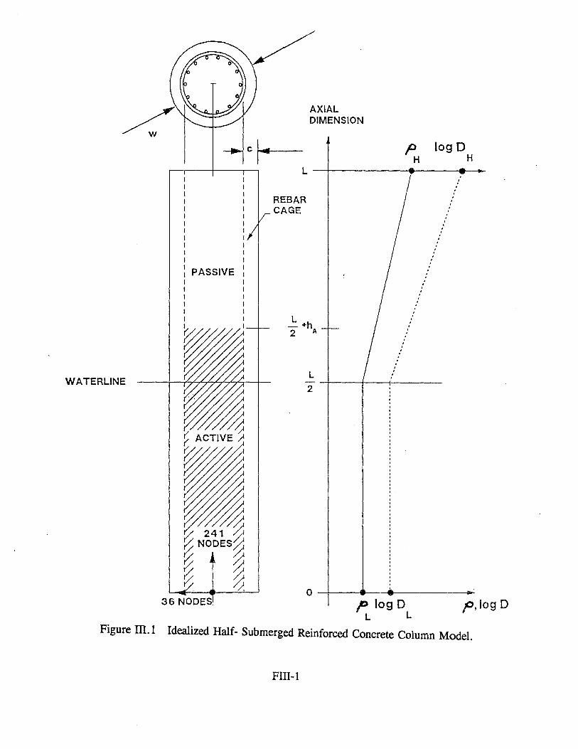
WATERLINE
Figure ill.l
I I I I I I I I I I 1 I I I I I I I 1 I I
·~
i) ~
%N~b~s~ % ~ % ~ ('; ~
36 NODES
L
AXIAL DIMENSION
REBAR CAGE
__!: +h 2 A
L -2
0
p H
: . . .
. . . .
. . ' . . ' . . . . . ' . ' . . . . . . . . . ' ' . . ' . . '
p log D L L
log D H
. . . . . .
. . . . . . . .
p,logD
Idealized Half- Submerged Reinforced Concrete Column Model.
FIII-1
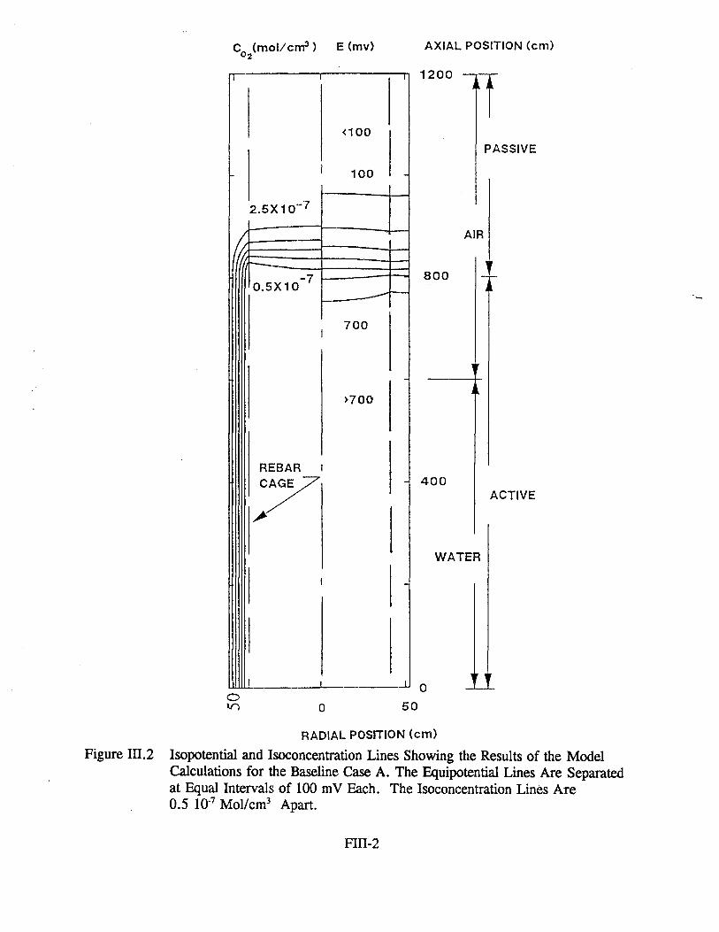
II I
I
2.5X1o-7
t (~t--
0.5X10⁻⁷
I
REBAR 1
7
0 VI
II
I
I
I
0
AXIAL POSITION (em)
I 1200
<100 PASSIVE
100 -
AIR
800 1-----
700
-
>700
400 ACTIVE
WATER
I 0
50
RADIAL POSITION (em)
Figure II1.2 Isopotential and lsoconcentration Lines Showing the Results of the Model Calculations for the Baseline Case A. The Equipotential Lines Are Separated at Equal Intervals of 100 mV Each. The Isoconcentration Lines Are 0.5 I0-7 Mollcm3 Apart.
FIII-2

-N
E ()
' < .... a_ ...1> w._. o_ ocn o:z ow <tO ~ ....
z w a: a: :::> 0
...... N
E ()
' ! >-1-
ocn -z Ow Oo z .... <z
w a: a: :::> 0
...... N
E ()
' ! Q >-0 !: 0 (/)
l: z 1- w <( 0 0
._. z w a: a: :::> 0
1
-0
B~SEA +-----------------=::...... -- :::::-::=--------1
--1 -
--2-
--3-
--4
0
--1 -
--2 -
--3-
--4-
--5
0.8
0.6
0.4
0.2
0.0 0 400
\ I
B '
CASE A \
1
B I ,, I
"' I I 1 CASE A I I I \ \ \
..... --800 1200
WATER AIR _j 1: ~----- ACTIVE-------_,.,..._ __ PASSIVE ---.j AXIAL POSITION (em)
Figure III.3 Current Density (Sum of Both Sides) Distributions Along the Rebar Cage for the Baseline Case A and for Case B (Higher Concrete Resistivity). The Macrocell Current Density (Top) is Equal to the Algebraic Sum of the Anodic (Center) and Cathodic (Bottom) Current Densities. The Absolute Values of the Corrosion Current Densities and the Oxygen Consumption Current Densities are Equal to Those of the Anodic and Cathodic Current Densities Respectively.
FIII-3

100 4---~-L~~~--~~~~~L--T-O~T~A~L-L~~L-~--~~~~
...... 1: u
' 1 ~ <t E "'
10
1
2 10
1corr
TOTAL 1macro
~ MA~
corr
3 10
p (ohm-em) L
4 10
5 10
6 10
Figure III.4 Total Corrosion and Macrocell Currents, and Maximum Corrosion Current Density (Sums of Both Sides) As a Function of Lowest Concrete Resistivity While Keeping the Other Parameters Constant (Results from Cases A,B,L and M).
Fll-4

10
1
-8 10
"' /
,." ,.
"' "' "'
_, ,.
/ ...
0'~/// ~r
-7 10
-6 10
0 (cm2 /sec) L
TOTAL 1corr
)
TOTAL 1m aero
-5 10
-4 10
Figure ill.5 Total Corrosion and Macrocell Currents, and Maximum Corrosion Current Density (Sums of Both Sides) As a Function of Lowest Concrete Diffusivity While Keeping the Size of the Active and Passive Regions Constant. The Solid Lines Correspond to the Cases With the Resistivity Range 2-10 KO-cm (A,F,G). The Dashed Lines Correspond to the Cases With the Resistivity Range 20.100 KO-cm (B,J and K).
Fill-5

60
-<(
E 40 -20
0
MAXI corr
~-- TOTAL I macro
100 200
HEIGHT OF ACTIVE ZONE ABOVE WATER (em)
8
300
Figure m.6 Total Corrosion and MacroceU Currents, and Maximum Corrosion Current Density (Sums of Both Sides), As a Function of Height of the Active Zone Above Water While Keeping the Other Magnitudes Constant (Cases A,C,D and E).
Fill-6

0 I I I I I I I I I
-CASE;;'/\ ~ 1\ -
..... N
E -2 -0
'-....
~ - c ->-1::
OUJ -z Ow -4-Oo z.,_ A <z w 0: -0: ::J 0
-6-
E
I I I I I I I I I
0 400 800 1200
AXIAL POSITION (em)
Figure III. 7 Distribution of the Corrosion Current Density (Sums of Both Sides) for the Cases Indicated in Figure III.6.
FIII-7

> E ;;:; 200 0 < lL a: :;) C/)
w CJ 400 < 0 .... < ...I < ~ 600 z w 1-0 0.
-a 10
740,..---- ----,
745 ABOVE WATER
aELOW WATER
1.0 1.2 1.4
(X 107 )
- 7 10
PASSIVE
CORROSION CURRENT DENSITY f#A/ cm2)
-6 10
tre m.s Composite Polarization Diagram Showing the Locus of Potential at the Cage Surface and Oxygen Consumption Current Density (Sum of Both Sides) As It Varies Along the Rebar Cage (Baseline Case A). The Portions of the Diagram Corresponding to Different Column Regions Are Indicated in the Main Plot and in the Detailed Inset.
Fill-S

6. GENERAL DISCUSSION
The findings of each Part of the project have been individually discussed in
each of the corresponding sections. This discussion addresses the mutual
implications of the findings and their general significance.
All Parts of the investigation have identified, by separate means, the presence of
significant macrocell action in marine substructure conditions. Substantial amounts of
cathodic reaction took place both at regions where the steel is passive and also in
portions of the chloride-contaminated concrete.
The findings of Part Ill suggest that much of the anodic reaction takes place
above water, peaking at a region just below the beginning of the passive-steel zone.
That prediction is also supported by the observation in the field of cracking and rusting
almost exclusively in the splash-evaporation zone. The laboratory columns in Part I
showed corrosion predominantly below water, and the columns used in Part II showed
most of the net anodic activity also below the waterline. That behavior does not
contradict the computer-model predictions because the laboratory columns were
operated with a very small portion below water. The behavior in that case approaches
an extension of Case 0 (Rgure 111.7), where the extent of anodic activity in the below
water portion is increased substantially by the relatively large amount of net cathodic
action existing above water. In addition, the computer calculations assume that a
mature active-passive pattern had developed in the column, which was not yet the
case for the columns of the Part I study by the end of the test period.
The results in Part II provided an estimation of the effective value of the oxygen
diffusion coefficient for water-saturated concrete (3 10-8 cm2 j sec). This supported
the choice of DL values used in the Part Ill computations. The relative importance of
the diffusivity of oxygen (as opposed to only concrete resistivity) in establishing the
overall extent of corrosion was emphasized by the findings of Part Ill. The laboratory
62

results in Part II provided experimental support for that prediction by showing that,
because of a reduction in oxygen supply, corrosion activity did not increase after
resistivity had decreased below a given amount.
For a given moisture condition, both oxygen transport, chloride transport and
electric conduction through concrete are affected by the quality of the concrete. The
interplay between concrete composition and transport parameters was illustrated by
the results in Part I. The concrete with the microsilica addition showed improved
behavior during relatively early ages. However, the advantage with respect to the
concrete with fly ash as the only pozzolanic component became less important as
both concretes aged. The model predictions from Part Ill suggest that the small
resistivity differences (between both concrete mixtures) that may exist after 2 or 3
years of operation, would only marginally affect the relative distribution of corrosion.
The results in Part I, showing essentially the same amount of macrocell current for
both concretes at the end of the test period, suggest that the oxygen transport in both
concretes are comparable. Longer-term monitoring of these columns will be
necessary to reveal possible differences in behavior.
7. CONCLUSIONS
7.1 PART I CONCLUSIONS
7 .1. 1 All laboratory test columns developed concrete resistivity patterns
consistent with concrete drying in the upper portions. The resistivity of the upper
portions of the control condition (fly ash concrete, no surface treatment) was
significantly reduced by periodic surface moisture application. The resistivity of the
columns in the silane and siloxane surface treatment groups was not affected by
periodic surface moisture application. The results indicated that in the upper regions
the surface treatments prevented water ingress but did not cause water to be retained.
63

7.1.2 The resistivity of concrete in the submerged portions of the columns reflected
the curing process and the type of concrete. The fly ash + microsilica (F + S)
concrete cured quickly compared with the fly ash-only (F) material. The initial values
of resistivity of the concrete mixtures corresponded to estimated rapid chloride
permeability Coulomb values of 800 C and 3,000 C for the F + S and F type materials.
After about two years of testing, both concretes had reached to similar levels of
resistivity in the submerged portions of the columns, corresponding to Coulomb values
of about 300 C. The resistivity of the concrete above water near the end of the 3-year
test period was much higher than below water, but similar for both concrete types.
7 .1.3 The steel below water in all test columns was initially in the active
condition, but it passivated over a period of about 150 days for the F + S concrete, and
about 100 days for the F concrete. The longer passivation time for the F + S concrete
may be due to lower pore water pH in that material.
7 .1.4 Activation of the steel below water took place after times of about 300
days for the F + S concrete and 150 days for the F concrete. The difference may
reflect primarily the early differences in curing behavior of both concretes. The-time-to
corrosion values agree with approximate calculations based on estimated diffusivity
from the resistivity measurements.
7 .1.5 Corrosion macro cell patterns developed on most columns with electronic
macrocell currents generating in the element below water and being consumed by the
element just above water. The amount of macrocell current was roughly the same for
both types of concrete, suggesting that the behavior is similar following the early
curing period.
7.1.6 Only 3 out of 12 columns had developed recognizable corrosion above
water after 3 years of testing. It is proposed that the element above water was being
partially cathodically protected by the submerged element, at least up the stage of
corrosion pattern evolution examined during the test duration.
64

7.2 PART II CONCLUSIONS
7.2.1 The test columns developed a corrosion pattern with a cathodic upper
portion (zone above water) and anodic regions in the chloride-rich areas.
7.2.2 The cathodic current in the upper column segments was strongly
affected by partial moisture application on the column zone above water. Cathodic
currents experienced dramatic proportional increases. The increase was due to the
reduction of ohmic potential drops in the corrosion macrocell system as a result of
moisture application.
7.2.3 Moisture saturation of the zones above water resulted in lesser ohmic
potential drops in the concrete and an increase of cathodic reduction currents in the
upper portions of the system. However, the cathodic currents (overall) experienced
limitation to a value consistent with concentration polarization of the oxygen reduction
reaction.
7.2.4 The value of the limiting current density for oxygen reduction corresponded to
an effective diffusion coefficient for oxygen in water-saturated concrete
(D-6 10'6 cm2 /sec) which is in agreement with values reported in the literature.
7.3 PART Ill CONCLUSIONS
7.3.1 In a simulated reinforced concrete marine substructure column, the
potential of the reinforcing steel varied continuously from the noble values in the zone
above water to very active values in the submerged zone.
65

7.3.2 The concentration of oxygen inside the column varied from a value near
equilibrium with the exterior at the top, to almost zero below water. Oxygen transport
to the steel below water was almost exclusively through the concrete cover and not
downward through the center of the column.
7.3.3 The corrosion current density was greatest at the top of the active zone
of the column. Corrosion below water proceeded at a smaller rate even though the
steel potential was significantly less noble than in the region of highest corrosion.
7.3.4 The local oxygen consumption rate was greatest near the top of the
active steel zone. This resulted from a combination of the oxygen diffusivity pattern
assumed in the calculations, and of the proximity of the active steel zone.
7.3.5 The total corrosion current varied from being almost equal to the total
macrocell current, to being several times greater, depending on the values of concrete
resistivity and oxygen diffusivity ranges assumed.
7 .3.6 Corrosion below water was not enhanced by oxygen consumption in the
air zone unless corrosion activity in the latter was greatly reduced.
7 .3. 7 The overall level of corrosion increased with increasing oxygen diffusivity
and reduced concrete resistivity.
7.3.8 Relative changes in oxygen diffusivity had a greater impact on corrosion
activity than comparable relative changes in concrete resistivity.
7.3.9 The three-dimensional, heterogenous nature of the system leads to
polarization behaviors that cannot be described by a simple monotonic polarization
curve.
66
7.4 GENERAL CONCLUSIONS
G 1. Preponderance of corrosion below water in laboratory experiments is caused by
the relative size of the submerged and free portions.
G2. The different approaches in the investigation provided results that confirmed the
importance of corrosion macrocells in the development of corrosion in substructure
columns.
G3. The overall results also indicated the importance of oxygen transport in
establishing the severity of corrosion in substructure conditions.
G4. Oxygen diffusivity (or another appropriate measure of oxygen transport) should
be considered as an important performance parameter for selection of concrete for
future design for corrosion control.
G5. Design that promotes moist concrete condition (as in submerged footers) is
recommended as a corrosion prevention/control approach.
67

8. STATEMENT OF BENEFITS
While this investigation addressed principally the propagation stage of
corrosion, the present emphasis on long term durability (design service lives of 75
years or more) underscores the importance of extending the initiation stage of
corrosion. Maintaining a thick concrete cover between the rebar and the external
environment is still the first item of concern in successful design for corrosion control
of marine substructure. A minimum cover of 4 in (10 em) enforced by inspection is
recommended whenever structurally feasible, to extend the length of the initiation
period of corrosion [111.1].
The findings from Part I are by themselves not sufficient to decide the issue of
whether microsilica addition is an economically desirable means of extending the
length of the initiation period of corrosion in marine substructure. The results
underscore the limitations of short term laboratory testing for evaluation of long term
concrete behavior, revealing the relatively slow reaction of fly ash as it affects
corrosion development. It is recommended that structures in the field be subject to
monitoring of chloride penetration profiles, paying special attention to the effect of age
on chloride ion transport.
All three parts of the project revealed the importance of oxygen transport
through the concrete in determining the extent of corrosion reactions. It is
recommended that measurements of oxygen diffusivity (or another suitable oxygen
transport parameter) under both a water-saturated and an intermediate-moisture
condition be made part of the testing used in the selection of future FOOT candidate
mix designs for improved corrosion control. Concrete resistivity measurements,
which can be easily performed instantaneously and non-destructively, should be
performed routinely both to obtain a quality descriptor of wet concrete and for field
investigations.
68

The findings also support structural design that promotes concrete moisture,
such as partially submerged footers as a opposed to exposed piling below footers,
to retard oxygen transport whenever possible. This type of design has the
advantage of facilitating future cathodic protection of the structure and permitting
the use of a thicker concrete cover than would be feasible in driven piles.


