
Fast Analysis of a Compound Large Reflector
Antenna
by
Stephanie Alphonse
Thesis presented in partial fulfilment of the requirements for
the degree of Master of Science in Engineering at
the University of Stellenbosch
Department of Electrical and Electronic Engineering,
University of Stellenbosch
Supervisors:Prof K.D. Palmer and Dr D.I.L de Villiers
March 2012

Declaration
By submitting this thesis electronically, I declare that the entirety of the work contained
therein is my own, original work, that I am the sole author thereof (save to the extent
explicitly otherwise stated), that reproduction and publication thereof by Stellenbosch Uni-
versity will not infringe any third party rights and that I have not previously in its entirety
or in part submitted it for obtaining any qualification.
Date: March 2012
Copyright ©2012 Stellenbosch University
All rights reserved.
i
Stellenbosch University http://scholar.sun.ac.za
Abstract
The offset Gregorian dual reflector antenna is eminently well suited to a radio telescope
antenna application as it offers a narrow beam width pattern (i.e high gain) and good
efficiency. The focus of this work is on the analysis of characteristics of such a Gregorian
antenna.
The design of the class of reflector antennas is normally based on the use of ray-optics,
with this simplified approach being able to predict antenna performance based on approx-
imate formulas for example the beam width against aperture size. However for compound
antennas such as the Gregorian reflector there are several interdependent parameters that
can be varied and this reduces the applicability of the simple ray-optic approach. It was
decided that, if a fast enough analysis of a configuration can be found, the technique of
design through interactive analysis would be viable.
To implement a fast analysis of the main beam performance of such a Gregorian antenna,
a solution algorithm has been implemented using a plane wave spectrum approach combined
with a custom aperture integration formulation. As this is able to predict the beam per-
formance within about a second on a PC, it is suitable for iterative design. To implement
the iterative design in a practical manner a user interface has been generated that allows
the user to interactively modify the geometry, see the physical layout, and then find the
antenna pattern. A complete working system has been realised with results comparing well
to a reference solution. The limitations of the technique, such as its inaccuracy in predicting
the side lobe structure, are also discussed.
ii
Stellenbosch University http://scholar.sun.ac.za

Opsomming
Die afset Gregoriaanse dubbelweerkaatser antenna is uiters gepas vir radioteleskoop toepass-
ings aangesien dit ’n nou bundelwydte (hoe aanwins) en ’n goeie benuttingsgraad bied. Die
fokus van hierdie werk is op die analise van die eienskappe van so ’n Gregoriaanse antenna.
Die ontwerp van die klas van weerkaatsantennas is normaalweg gebaseer op straal-optika,
waar hierdie vereenvoudigde tegniek, deur benaderde formules, gebruik kan word om an-
tennawerkverrigting af te skat soos bv. die bundelwydte teen stralingsvlakgrootte. Vir
saamgestelde antennas soos die Gregoriaanse weerkaatser is daar egter verskeie onafhank-
like parameters wat verstel kan word en die toepaslikheid van die eenvoudige straal-optiese
benadering verminder. Dit was besluit dat, indien die analise van die konfigurasie vinnig
genoeg uitgevoer kon word, die tegniek van ontwerp deur interaktiewe analise werkbaar kan
wees.
Om ’n vinnige analise van die hoofbundelwerkverrigting van so ’n Gregoriaanse antenna te
bewerkstellig, is ’n oplossingsalgoritme gemplementeer wat gebruik maak van ’n platvlakgolf-
spektrum benadering in kombinasie met ’n doelgemaakte stralingsvlakintegrasieformulering.
Aangesien hierdie strategie die hoofbundel binne ongeveer ’n sekonde op ’n persoonlike reke-
naar kan voorspel, is dit gepas vir iteratiewe ontwerp. Om die iteratiewe ontwerp op ’n
praktiese wyse te implementeer is ’n gebruikerskoppelvlak geskep wat die gebruiker toelaat
om, op ’n interaktiewe wyse, die geometrie aan te pas, die fisiese uitleg te sien en dan die
stralingspatroon te bereken. ’n Volledige werkende stelsel is gerealiseer met resultate wat
goed ooreenstem met ’n verwysingsoplossing. Die tekortkominge van die tegniek, soos die
onakkuraatheid in die voorspelling van die sylobstruktuur, word ook bespreek.
iii
Stellenbosch University http://scholar.sun.ac.za

Acknowledgements
I would like to express my gratitude to the following people and organisations for their
contribution towards this project:
My academic supervisors Prof. Keith D. Palmer and Dr Dirk I.L. de Villiers for their
comprehensive and invaluable guidance in completing this work.
Prof. Howard Reader for his confidence in me and the suggestion to attend various
electromagnetic courses.
Prof. Gerard Rambolamanana for his guidance and advice to adjust my watch to be
on time.
Hasimboahangy Samuel R. for her love and patience.
Anita van der Spuy for her proofreading of this report.
EMSS for the use of FEKO software which they made available for simulation purposes.
The South African SKA project for the financial support during my Masters.
Last but not the least to my family in Madagascar for their love, support and encour-
agements during the last two and half years.
”In the middle of difficulty lies opportunity” Albert Einstein.
iv
Stellenbosch University http://scholar.sun.ac.za

To my nephews: Joe-Georgio A., Jean-Yves Alphonse A.and nieces: Erwine Trishilla A., Marie-Joanna A.
v
Stellenbosch University http://scholar.sun.ac.za
Contents
Declaration i
Abstract ii
Opsomming iii
Acknowledgements iv
Table of contents vi
List of figures ix
List of tables xi
Nomenclature xiii
1 Introduction 1
1.1 Background to the Project . . . . . . . . . . . . . . . . . . . . . . . . . . . . 1
1.2 Objectives and Outline of this Thesis . . . . . . . . . . . . . . . . . . . . . . 2
2 General Theory of Reflector Antennas 3
2.1 Types of reflector antennas . . . . . . . . . . . . . . . . . . . . . . . . . . . . 4
2.1.1 Single reflector . . . . . . . . . . . . . . . . . . . . . . . . . . . . . . 4
2.1.2 Dual reflector . . . . . . . . . . . . . . . . . . . . . . . . . . . . . . . 5
2.2 Directivity and Gain: . . . . . . . . . . . . . . . . . . . . . . . . . . . . . . . 6
2.2.1 Principles of a paraboloid reflector . . . . . . . . . . . . . . . . . . . 7
2.2.2 Directivity: . . . . . . . . . . . . . . . . . . . . . . . . . . . . . . . . 8
2.2.3 Gain of the reflector antenna: . . . . . . . . . . . . . . . . . . . . . . 9
2.3 Aperture efficiency ηap: . . . . . . . . . . . . . . . . . . . . . . . . . . . . . . 9
2.3.1 Illumination efficiency ηt: . . . . . . . . . . . . . . . . . . . . . . . . . 11
2.3.2 The spillover efficiency ηs: . . . . . . . . . . . . . . . . . . . . . . . . 12
2.3.3 The polarization efficiency ηpol: . . . . . . . . . . . . . . . . . . . . . 13
vi
Stellenbosch University http://scholar.sun.ac.za

Contents
2.3.4 The phase efficiency ηφ: . . . . . . . . . . . . . . . . . . . . . . . . . 13
2.3.5 The surface error efficiency ηr: . . . . . . . . . . . . . . . . . . . . . . 14
2.4 Summary . . . . . . . . . . . . . . . . . . . . . . . . . . . . . . . . . . . . . 14
3 High-frequency Methods for Reflector Antennas 15
3.1 Radiation structures . . . . . . . . . . . . . . . . . . . . . . . . . . . . . . . 15
3.1.1 Radiation current source . . . . . . . . . . . . . . . . . . . . . . . . . 16
3.1.2 Aperture distribution source . . . . . . . . . . . . . . . . . . . . . . . 18
3.2 Geometric Optics theory . . . . . . . . . . . . . . . . . . . . . . . . . . . . . 20
3.2.1 Propagation of rays in Geometrical Optics . . . . . . . . . . . . . . . 21
3.2.2 Reflection on the boundary . . . . . . . . . . . . . . . . . . . . . . . 22
3.2.3 Propagation power of the rays . . . . . . . . . . . . . . . . . . . . . 23
3.3 Physical Optics theory . . . . . . . . . . . . . . . . . . . . . . . . . . . . . . 23
3.3.1 Induced current density for PEC . . . . . . . . . . . . . . . . . . . . 24
3.3.2 PO radiation fields . . . . . . . . . . . . . . . . . . . . . . . . . . . . 24
3.3.3 Dual-reflector application . . . . . . . . . . . . . . . . . . . . . . . . 25
3.4 Analysis of the diffraction effect on the sub-reflector rim . . . . . . . . . . . 26
3.4.1 Huygens-Fresnel principle of diffraction . . . . . . . . . . . . . . . . . 26
3.4.1.1 Edge diffraction in the sub-reflector surface . . . . . . . . . 27
3.4.2 Geometrical Theory of Diffraction . . . . . . . . . . . . . . . . . . . . 28
3.4.2.1 Geometrical Optics fields . . . . . . . . . . . . . . . . . . . 28
3.4.2.2 Diffracted fields on a curved surface . . . . . . . . . . . . . 28
3.4.3 Physical Theory of Diffraction . . . . . . . . . . . . . . . . . . . . . . 31
3.4.3.1 Method of Equivalent Current . . . . . . . . . . . . . . . . . 32
3.5 Antenna Radiation pattern using Plane Wave Spectrum . . . . . . . . . . . . 32
3.5.1 Plane waves spectrum representation . . . . . . . . . . . . . . . . . . 33
3.5.2 The Angular spectrum approximation . . . . . . . . . . . . . . . . . . 34
3.6 Conclusion . . . . . . . . . . . . . . . . . . . . . . . . . . . . . . . . . . . . . 35
4 Description of a Gregorian Reflector Antenna and Creation of a FEKO
Reference 36
4.1 Description of the Gregorian Reflector Antenna . . . . . . . . . . . . . . . . 37
4.1.1 Gregorian geometry structure . . . . . . . . . . . . . . . . . . . . . . 37
4.1.2 Main Reflector . . . . . . . . . . . . . . . . . . . . . . . . . . . . . . 38
4.1.2.1 Characteristics of the Main Reflector . . . . . . . . . . . . . 38
4.1.2.2 Main reflector parameters . . . . . . . . . . . . . . . . . . . 38
4.1.3 Sub-reflector . . . . . . . . . . . . . . . . . . . . . . . . . . . . . . . . 39
4.1.3.1 Characteristics of the sub-reflector . . . . . . . . . . . . . . 39
vii
Stellenbosch University http://scholar.sun.ac.za

Contents
4.1.3.2 Reflection from the sub-reflector . . . . . . . . . . . . . . . 40
4.1.4 Equivalent parabola analysis . . . . . . . . . . . . . . . . . . . . . . . 41
4.1.5 Antenna design parameters . . . . . . . . . . . . . . . . . . . . . . . 42
4.1.5.1 Ellipsoid parameters . . . . . . . . . . . . . . . . . . . . . . 42
4.1.5.2 Paraboloid design parameters . . . . . . . . . . . . . . . . . 44
4.2 Creation of a Gregorian antenna Reference in FEKO . . . . . . . . . . . . . 45
4.2.1 The system feed . . . . . . . . . . . . . . . . . . . . . . . . . . . . . . 45
4.2.1.1 Simulation in FEKO . . . . . . . . . . . . . . . . . . . . . . 45
4.2.1.2 Method Of Moments . . . . . . . . . . . . . . . . . . . . . . 46
4.2.1.3 Results gain of the feed . . . . . . . . . . . . . . . . . . . . 46
4.2.1.4 Advantages of using a dual reflector . . . . . . . . . . . . . 47
4.2.2 Gregorian reflector antenna simulation using hybrid technique . . . . 48
4.2.2.1 FEKO simulation set-up . . . . . . . . . . . . . . . . . . . . 49
4.2.2.2 Feed pattern description . . . . . . . . . . . . . . . . . . . . 49
4.2.2.3 Sub-reflector pattern . . . . . . . . . . . . . . . . . . . . . . 50
4.2.2.4 Radiation pattern of the Gregorian antenna system . . . . . 51
4.3 Conclusion . . . . . . . . . . . . . . . . . . . . . . . . . . . . . . . . . . . . . 53
5 Fast Approximation Technique for Reflector Antenna Patterns 54
5.1 Radiation pattern of the sub-reflector using PWS . . . . . . . . . . . . . . . 55
5.2 Radiation of the main reflector . . . . . . . . . . . . . . . . . . . . . . . . . . 59
5.2.1 Aperture Integral Technique . . . . . . . . . . . . . . . . . . . . . . . 59
5.2.2 Gauss Legendre technique . . . . . . . . . . . . . . . . . . . . . . . . 60
5.3 Comparison of the fast approximation results with FEKO . . . . . . . . . . . 62
5.4 Matlab GUI application . . . . . . . . . . . . . . . . . . . . . . . . . . . . . 66
5.4.1 Overview of the GUI . . . . . . . . . . . . . . . . . . . . . . . . . . . 66
5.4.2 GUI design . . . . . . . . . . . . . . . . . . . . . . . . . . . . . . . . 67
5.4.2.1 Input parameters . . . . . . . . . . . . . . . . . . . . . . . . 67
5.4.2.2 Computation of results . . . . . . . . . . . . . . . . . . . . . 67
5.4.2.3 Plots of the Geometry and Pattern . . . . . . . . . . . . . . 68
5.5 Conclusion . . . . . . . . . . . . . . . . . . . . . . . . . . . . . . . . . . . . . 68
6 Conclusions 69
Bibliography 70
A Analytical evaluation of directivity using spectrum [1]. A–1
A.1 Directivity using PWS . . . . . . . . . . . . . . . . . . . . . . . . . . . . . . A–1
A.2 The total radiated power . . . . . . . . . . . . . . . . . . . . . . . . . . . . . A–2
viii
Stellenbosch University http://scholar.sun.ac.za

List of Figures
1.1 Prototype of a dual offset Gregorian dual reflector antenna for MeerKAT . . 2
2.1 Types of reflector antenna . . . . . . . . . . . . . . . . . . . . . . . . . . . . 4
2.2 Paraboloid single reflector antena . . . . . . . . . . . . . . . . . . . . . . . . 5
2.3 Geometry of two types of dual reflector antenna . . . . . . . . . . . . . . . . 6
2.4 Geometry of parabolic reflector . . . . . . . . . . . . . . . . . . . . . . . . . 7
2.5 Aperture efficiency for different feed patterns as function of θ0 . . . . . . . . 11
2.6 Taper or illumination efficiency for different feed patterns as function of θ0 . 11
2.7 Spillover efficiency for different feed patterns . . . . . . . . . . . . . . . . . . 12
2.8 Trade-off between spillover and taper efficiencies . . . . . . . . . . . . . . . . 13
3.1 Distribution of currents on a reflector surface . . . . . . . . . . . . . . . . . . 17
3.2 Radiation fields on a reflector aperture plane . . . . . . . . . . . . . . . . . . 19
3.3 Primary and secondary wave of radiated wave . . . . . . . . . . . . . . . . . 21
3.4 Derivation from Snell’s Law . . . . . . . . . . . . . . . . . . . . . . . . . . . 22
3.5 Offset Gregorian dual reflector coordinate . . . . . . . . . . . . . . . . . . . 25
3.6 Huygens construction . . . . . . . . . . . . . . . . . . . . . . . . . . . . . . . 26
3.7 Rays diffracted in the parabolic reflector edges . . . . . . . . . . . . . . . . . 27
3.8 Diffracted rays at a curved edge . . . . . . . . . . . . . . . . . . . . . . . . . 29
3.9 Coordinate system of the plane wave propagation . . . . . . . . . . . . . . . 33
4.1 Front and side view of a Gregorian dual reflector . . . . . . . . . . . . . . . . 37
4.2 Ellipsoid geometry . . . . . . . . . . . . . . . . . . . . . . . . . . . . . . . . 40
4.3 Equivalent paraboloid of a dual offset Gregorian geometry with circular aperture 41
4.4 An offset Gregorian dual reflector antenna geometry . . . . . . . . . . . . . . 45
4.5 Ideal source oriented towards a paraboloid reflector with the diameter of the
dish D = 50λ, generated with FEKO . . . . . . . . . . . . . . . . . . . . . . 46
4.6 Comparison of approximate gain from the full-wave results from FEKO and
the analytical approximation for different sources . . . . . . . . . . . . . . . 47
4.7 Model in 3D of an Offset Gregorian Dual reflector . . . . . . . . . . . . . . 48
ix
Stellenbosch University http://scholar.sun.ac.za

List of Figures
4.8 Idealised feed pattern . . . . . . . . . . . . . . . . . . . . . . . . . . . . . . . 50
4.9 3D geometry of the sub-reflector . . . . . . . . . . . . . . . . . . . . . . . . . 50
4.10 Radiation pattern of a 16.67λ sub-reflector for different frequencies . . . . . 51
4.11 3D geometry of the paraboloid of the dish . . . . . . . . . . . . . . . . . . . 52
4.12 Radiation pattern of an offset Gregorian dual reflector antenna in H and E-
plane for f/D=0.3333 . . . . . . . . . . . . . . . . . . . . . . . . . . . . . . . 52
4.13 Radiation pattern of an offset Gregorian dual reflector antenna in H and E-
plane for f/D=0.65 . . . . . . . . . . . . . . . . . . . . . . . . . . . . . . . . 53
5.1 Rectangular mesh grid of the cut surface of the ellipsoid sub-reflector . . . . 56
5.2 Front and side view of the aperture E-field on the sub-reflector . . . . . . . . 57
5.3 Cut-off field on the sub-reflector aperture . . . . . . . . . . . . . . . . . . . . 57
5.4 Diffraction term on the sub-reflector aperture . . . . . . . . . . . . . . . . . 58
5.5 Diffraction term back transformed at the origin . . . . . . . . . . . . . . . . 58
5.6 Top and side view of the sub-reflector cut radiation pattern . . . . . . . . . . 59
5.7 Orientation of the new source towards the Main reflector . . . . . . . . . . . 60
5.8 Radiation pattern of the reflector for 1 GHz frequency using PWS approach 61
5.9 Radiation pattern of the reflector for 1.25 GHz frequency using PWS approach 62
5.10 Radiation pattern of the reflector for 2 GHz frequency using PWS approach 62
5.11 Comparison of the fast approximation technique and the numerical simulation
of the dual reflector radiation pattern in E- and H-plane at freq= 1 GHz . . 63
5.12 Comparison of the fast approximation technique and the numerical simulation
of the dual reflector radiation pattern in E- and H-plane at freq= 1.25 GHz . 64
5.13 Comparison of the fast approximation technique and the numerical simulation
of the dual reflector radiation pattern in E- and H-plane at freq= 2 GHz . . 65
5.14 A quick visualisation of Gregorian dual reflector properties . . . . . . . . . . 67
x
Stellenbosch University http://scholar.sun.ac.za

List of Tables
4.1 Gregorian design parameters . . . . . . . . . . . . . . . . . . . . . . . . . . . 38
4.2 Parameter Values computed from the design equations . . . . . . . . . . . . 44
4.3 Parameters of the antenna design . . . . . . . . . . . . . . . . . . . . . . . . 49
5.1 Comparison of the beamwidth results . . . . . . . . . . . . . . . . . . . . . . 66
xi
Stellenbosch University http://scholar.sun.ac.za

Nomenclature
List of abbreviations
2D Two dimensional
CAD Computer-aided Design
CEM Computational Electromagnetic
GO Geometrical Optics
GTD Geometrical Theory of Diffraction
GUI Graphical User Interface
HF High frequency
HPBW Half Plane Beam Width
MEC Method of Equivalent Current
MeerKAT Karoo Array Telescope
MLFMM Multilevel Fast Multipole Method
MoM Method of Moments
PEC Perfect Electric Conductor
PO Physical Optics
PTD Physical Theory of Diffraction
PWS Plane Wave Spectrum
rms Root Mean Square
SKA Square Kilometre Array
SLL Side Lobe Level
uicontrol User Interface Control
uimenu User Interface Menu
VSWR Voltage Signal Noise Ratio
Constants and Units
ε,ε0 General and free space permittivity F/m
η intrinsic impedance of free space (η =√
µ0ε0
) Ω
xii
Stellenbosch University http://scholar.sun.ac.za

Nomenclature
λ wavelength m
µ,µ0 General and free space permeability H/m
k0 wave number in free space rad.s−1
w angular frequency rad/s−1
Symbols and Units
A Electric vector potential Wb/m
Am Magnetic vector potential W/m2
B Magnetic flux density Wb/m2
D Electric flux density C/m2
E Electric field intensity (spatial form) V/m
H Magnetic field intensity (spatial form) A/m
J ,Jm Electric and magnetic currents A
Jes,Jms Electric and magnetic current densities A/m2
S Time average Poynting vector V
xiii
Stellenbosch University http://scholar.sun.ac.za

Chapter 1
Introduction
1.1 Background to the Project
It is hoped that the innovation of designing a powerful radio telescope, which will operate
over a wide microwave frequency range, scan and map the sky with 50-100 times more
sensitivity than any present-day radio telescope, has been entrusted to the South Africa
Square Kilometre Array(SKA SA) project [2]. This large telescope is intended to solve vari-
ous problems experienced by astronomers, cosmologists and other scientists and to determine
the nature of dark matter or dark energy [3].
The MeerKAT project, which is a precursor of the SKA, is adopting a new antenna
geometry to increase the efficiency of the reflectors. This new design, the offset Gregorian
dual reflector antenna, illustrated in Figure 1.1, is a solution to feed blockage limitations of
the preceding telescope. The MeerKAT will install an array of 64 of these antennas in South
African site, each of them having a primary reflector with a diameter of 13.5m and a smaller
concave secondary reflector. This antenna geometry with its clear optical path and low side
lobe level results, will propably be the geometry adopted for the SKA [4]. Most commercial
software package tools cannot analyse such large antennas efficiently due to the excessive
computational time and memory storage constraints. Finding a fast approximate solution is
thus the focus of the work.
1
Stellenbosch University http://scholar.sun.ac.za

Chapter 1. Introduction
Figure 1.1: Prototype of a dual offset Gregorian dual reflector antenna for MeerKAT [3]
1.2 Objectives and Outline of this Thesis
The offset dual reflector antennas are very popular because they offer good pattern perfor-
mance with low side lobes and high efficiency. As these are best suited to high gain antennas,
they are electrically large and their design can be based on ray-optics where all secondary
effects such as diffraction are ignored. The main objective of this thesis is to devise a scheme
that will allow for iterative design of an offset Gregorian reflector antenna. For that, a fast
quasi-analytical technique will be presented that will be shown to predict main beam per-
formance well. This technique allows the user to evaluate the design quickly enough on a
PC and develops an understanding of effect of the geometrical parameters on the antenna
performance.
A number of a sub-objectives are set to reach this objective:
1. Chapter 2 gives a brief introduction of reflector antennas
2. Some of the high frequency techniques that can be used with such a large antenna to
speed up the solution are discussed in Chapter 3
3. Section 4.1 introduces the description and design parameters of an offset Gregorian
dual reflector antenna;
4. Section 4.2 discusses the creation of a reference solution for a specific geometry using
the FEKO commercial software, so as to have a solution to which approximate solution
can be compared.
5. Chapter 5 describes an implementation of a suitable fast method of finding a Gregorian
radiation pattern and its full solution.
All numerical computation and results are obtained using DELL computer, equipped
with a dual core processor working at 3 GHz and with 4GB of RAM.
2
Stellenbosch University http://scholar.sun.ac.za
Chapter 2
General Theory of Reflector Antennas
Introduction
An antenna is a transducer device that converts a guided electromagnetic wave on
a transmission line into a plane wave radiating in free space[5]. Various types of
antennas are used in radar or satellite communication. The most widely used for narrow
beam antenna are reflector antennas.
These antennas are composed basically of a primary feed and one or several reflectors
where the reflectors shape or deflect the radiation from the primary feed source which may
typically be a horn, dipole or microstrip antenna. Horns are commonly used for radio
telescopes because they provide a suitable symmetrical pattern, high efficiency, low VSWR
(with waveguide feeds) and relatively wide bandwidth. Diverse geometrical configurations of
reflector antennas can be seen in practice but the conventional reflector designs are planar,
corner or curved reflector, as depicted in Figure 2.1. The radiation pattern of the antenna
system is affected by several parameters such as the radiation pattern of the feed, the shape
and the size of the reflectors which can give rise to spillover, diffraction and the aperture
blockage effect.
This chapter highlights the paraboloid reflector geometry. Types of reflector antennas
are described in section2.1 and the parameters of the antenna are investigated in section2.2
and 2.3 respectively.
3
Stellenbosch University http://scholar.sun.ac.za

Chapter 2. General Theory of Reflector Antennas
(a) (b) (c)
Figure 2.1: Geometry of (a) aperture distributioncorner reflector, (b) plane reflector and (c)parabolic curved reflector after [6]
2.1 Types of reflector antennas
Reflector antennas are pencil beam antennas that may have one or more reflectors with the
larger reflector often shaped with a paraboloid. The paraboloid transforms a spherical wave
radiated by the feed located at the antenna focal point into a plane wave. Because of this
geometrical property, paraboloidal reflector antennas find application where a high gain is
desired, typically 30-40 dB, along with low cross polarization [7].
The number of reflectors used depends upon the application and also on the extent to
which it is necessary to optimise the efficiency of the antennas. Both dual and single reflectors
find application in radar and satellite communication. The next section will discuss the
characteristics and application of single and dual reflector antennas.
2.1.1 Single reflector
A single reflector antenna consists of a primary feed and a reflector facing it. The single
reflector antenna can be symmetrically fed from the reflector focal point or offset fed, as
illustrated on 2.2. Reflector surfaces are based on the conic sections: paraboloid, hyperboloid
or ellipsoid. Paraboloid reflectors are the simplest for narrow beamwidth, while ellipsoidal
and hyperboloidal sub-reflectors are usually applied to relocate focal points in quasi-optical
systems.
4
Stellenbosch University http://scholar.sun.ac.za
Chapter 2. General Theory of Reflector Antennas
(a) (b)
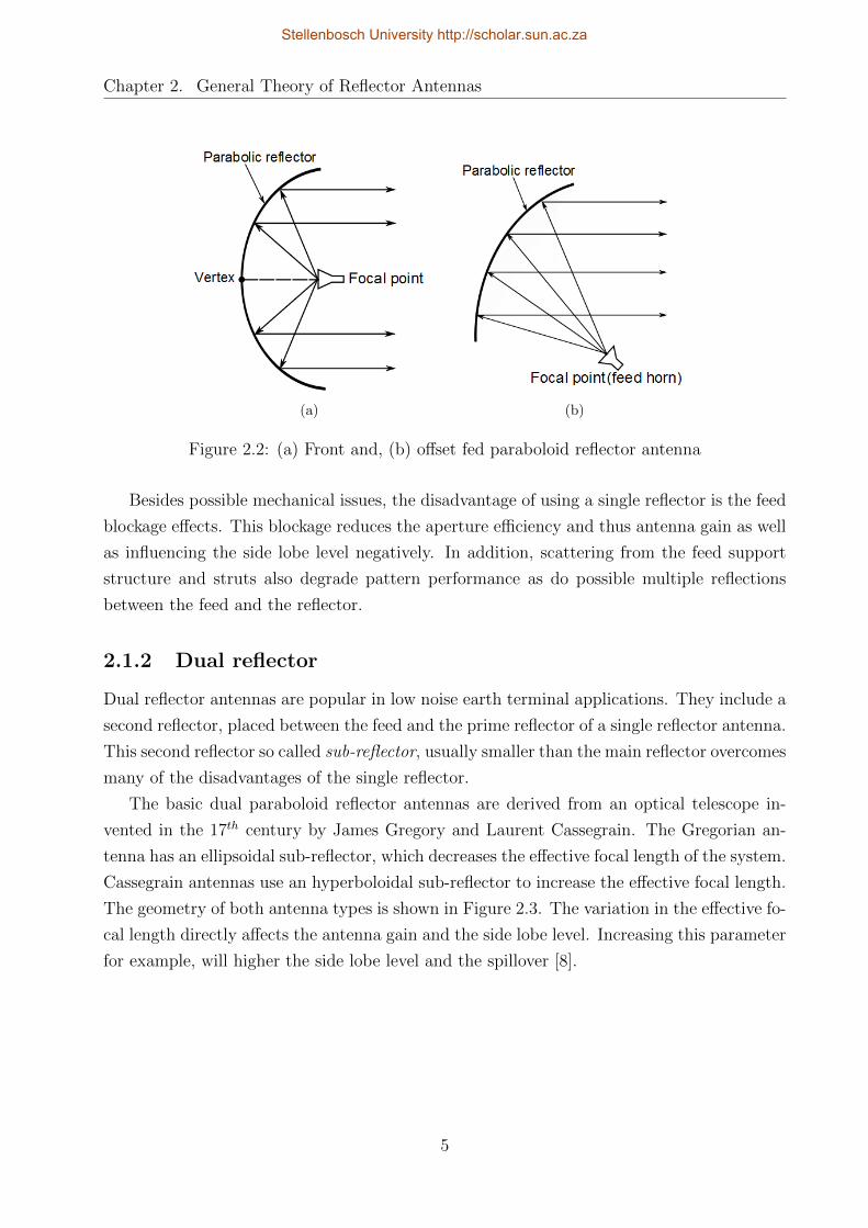
Figure 2.2: (a) Front and, (b) offset fed paraboloid reflector antenna
Besides possible mechanical issues, the disadvantage of using a single reflector is the feed
blockage effects. This blockage reduces the aperture efficiency and thus antenna gain as well
as influencing the side lobe level negatively. In addition, scattering from the feed support
structure and struts also degrade pattern performance as do possible multiple reflections
between the feed and the reflector.
2.1.2 Dual reflector
Dual reflector antennas are popular in low noise earth terminal applications. They include a
second reflector, placed between the feed and the prime reflector of a single reflector antenna.
This second reflector so called sub-reflector, usually smaller than the main reflector overcomes
many of the disadvantages of the single reflector.
The basic dual paraboloid reflector antennas are derived from an optical telescope in-
vented in the 17th century by James Gregory and Laurent Cassegrain. The Gregorian an-
tenna has an ellipsoidal sub-reflector, which decreases the effective focal length of the system.
Cassegrain antennas use an hyperboloidal sub-reflector to increase the effective focal length.
The geometry of both antenna types is shown in Figure 2.3. The variation in the effective fo-
cal length directly affects the antenna gain and the side lobe level. Increasing this parameter
for example, will higher the side lobe level and the spillover [8].
5
Stellenbosch University http://scholar.sun.ac.za
Chapter 2. General Theory of Reflector Antennas
(a) (b)
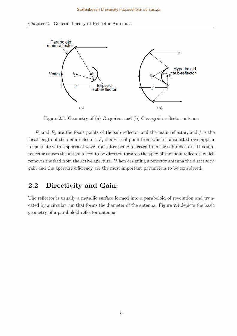
Figure 2.3: Geometry of (a) Gregorian and (b) Cassegrain reflector antenna
F1 and F2 are the focus points of the sub-reflector and the main reflector, and f is the
focal length of the main reflector. F1 is a virtual point from which transmitted rays appear
to emanate with a spherical wave front after being reflected from the sub-reflector. This sub-
reflector causes the antenna feed to be directed towards the apex of the main reflector, which
removes the feed from the active aperture. When designing a reflector antenna the directivity,
gain and the aperture efficiency are the most important parameters to be considered.
2.2 Directivity and Gain:
The reflector is usually a metallic surface formed into a paraboloid of revolution and trun-
cated by a circular rim that forms the diameter of the antenna. Figure 2.4 depicts the basic
geometry of a paraboloid reflector antenna.
6
Stellenbosch University http://scholar.sun.ac.za
Chapter 2. General Theory of Reflector Antennas
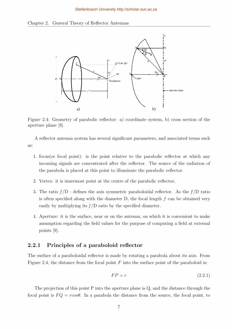
Figure 2.4: Geometry of parabolic reflector: a) coordinate system, b) cross section of theaperture plane [8].
A reflector antenna system has several significant parameters, and associated terms such
as:
1. focus(or focal point): is the point relative to the parabolic reflector at which any
incoming signals are concentrated after the reflector. The source of the radiation of
the parabola is placed at this point to illuminate the parabolic reflector.
2. Vertex: it is innermost point at the centre of the parabolic reflector,
3. The ratio f /D : defines the axis symmetric paraboloidal reflector. As the f /D ratio
is often specified along with the diameter D, the focal length f can be obtained very
easily by multiplying its f /D ratio by the specified diameter.
4. Aperture: it is the surface, near or on the antenna, on which it is convenient to make
assumption regarding the field values for the purpose of computing a field at external
points [9].
2.2.1 Principles of a paraboloid reflector
The surface of a paraboloidal reflector is made by rotating a parabola about its axis. From
Figure 2.4, the distance from the focal point F into the surface point of the paraboloid is:
FP = r (2.2.1)
The projection of this point P into the aperture plane is Q, and the distance through the
focal point is FQ = rcosθ. In a parabola the distance from the source, the focal point, to
7
Stellenbosch University http://scholar.sun.ac.za

Chapter 2. General Theory of Reflector Antennas
the point Q via the reflector is the same for all points Q.
FP + FQ = 2f (2.2.2)
By replacing the FP and PQ by their values, then (2.2.2) becomes:
r + rcosθ = 2f (2.2.3)
or
r =2f
1 + cosθ= fsec2
(θ
2
)with θ ≤ θ0 (2.2.4)
Equation (2.2.4) defines the paraboloid equation in spherical coordinates (r,θ,φ), and only
a function of the angle θ because of the rotational symmetry. It can also expressed in
rectangular coordinates:
r′2 = 4f(f− z)with r′ ≤ Q (2.2.5)
Another important parameter on the paraboloid is the reflector angle called the subtended
angle of the reflector θ0.
tan(θ0) =
(D2
)z
(2.2.6)
where z is the distance on the z axis from the focal point into the edge of the paraboloid
reflector and D is the diameter of the dish. This angle can also be expressed in another form
f/ D. It describes the curvature of the paraboloid and typically ranges from 0.3 to 1 [8].
f =D
4cot
(θ0
2
)(2.2.7)
2.2.2 Directivity:
Directivity is the ratio of the radiation intensity in the (θ, φ) direction to the average
radiation intensity over all directions. The average radiation intensity is equal to the total
power radiated divided by 4π [10].
The focal length f determines how the power from the feed is spread over the aperture
plane. If Gf (θ, φ) is the feed pattern, which is assumed to be circularly symmetric to simplify
the analysis, it has no component on the φ angle. The directivity of the reflector antenna
can be written as:
D =U(θ, φ)
U(θ, φ)av=
4πU(θ = π)
Pt(2.2.8)
where Pt is the total radiated power in [W] and U is the radiation intensity in [W/unit solid
8
Stellenbosch University http://scholar.sun.ac.za

Chapter 2. General Theory of Reflector Antennas
angle]. It can also be expressed in terms of the feed pattern as [6]:
D =16π2
λ2f2
∣∣∣∣∣∣θ0∫
0
√Gf (θ)tan(
θ
2)dθ
∣∣∣∣∣∣2
(2.2.9)
where λ is the wavelength.
2.2.3 Gain of the reflector antenna:
It is difficult to find the total power radiated by the antenna in practice; however, a parameter
of interest is the ability of the antenna to transform the available power at its input terminal
to the radiated power. This quantity is defined as the gain of the antenna. It is the ratio
of the radiation intensity in a given direction from the antenna to the total input power
accepted by the antenna per unit solid angle.
G(θ, φ) =4πU(θ = π)
Pin(2.2.10)
where U(θ = π) expresses the radiation intensity only on θ angle, because of the symmetrical
axis, and Pin is the input power radiated by the antenna.
The relationship between the power gain and the directivity of an antenna can be given
by comparing (2.2.8) and (2.2.10):
G(θ, φ) =PtPin
D(θ, φ) = ηradD(θ, φ) (2.2.11)
ηrad is the radiated efficiency of the antenna, the ratio of the total radiation power to the
input power radiated by the antenna. This factor is generally greater than 0 and less than
1 (0 ≤ ηrad ≤ 1). The radiation efficiency of the reflector antennas refers to ohmic losses
because the parabolic reflector is typically metallic, with a high conductivity. Another
efficiency factor, which relates the directivity of the system to that an uniform aperture at
same size is the aperture efficiency. Details of this factor will be discussed in the subsequent
section.
2.3 Aperture efficiency ηap:
The aperture efficiency can be decomposed into sub-efficiencies composed of the illumination
efficiency ηt , the spillover efficiency ηs, the phase efficiency ηφ, the polarization efficiency
ηpol and the surface error efficiency ηr [11]. Thus, the total aperture efficiency is the product
9
Stellenbosch University http://scholar.sun.ac.za

Chapter 2. General Theory of Reflector Antennas
of these factors which can be written as:
ηap = ηtηsηφηpolηr (2.3.1)
ηap varies with the position and the pattern of the feed. A class of the radiation pattern
is defined by Silver in literature as [12]:
Gf (θ) =
G
(n)0 cosn(θ) 0 ≤ θ ≤ π
2
0 π2≤ θ ≤ π
(2.3.2)
where n is a positive integer (n ≥ 1), G(n)0 is a constant for a given n and is determined
from the relation [6]: ∫∫S
Gf (θ)dΩ =
∫∫S
Gf (θ)dθdφ = 4π (2.3.3)
From this the constant G(n)0 can be computed:
π/2∫0
G(n)0 cosn(θ)sinθdθ = 2 (2.3.4)
where
G(n)0 = 2(n+ 1) (2.3.5)
and hence, the feed pattern in (2.3.2) becomes:
Gf (θ) =
2(n+ 1)cosn(θ) 0 ≤ θ ≤ π
2
0 π2≤ θ ≤ π
(2.3.6)
The aperture efficiency is expressed in terms of the radiation feed pattern of the antenna
as [6]:
ηap = cot
(θ
2
)2
∣∣∣∣∣∣θ0∫
0
√Gf (θtan
(θ
2
)dθ
∣∣∣∣∣∣2
(2.3.7)
θ0 is the half-angle of the reflector for a single reflector. An example calculation of
aperture efficiency for a paraboloid reflector design is shown in Figure 2.5. The result shows
that for each θ0, which is a function of f /D ratio, there is a value for n that maximizes the
aperture efficiency. The diameter D is of primary concern for the design. Clearly it should
be made as large as possible so that the physical aperture is maximized, but as it is one of
the primary cost drivers where compromise must be made.
10
Stellenbosch University http://scholar.sun.ac.za
Chapter 2. General Theory of Reflector Antennas
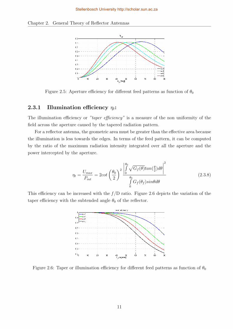
Figure 2.5: Aperture efficiency for different feed patterns as function of θ0
2.3.1 Illumination efficiency ηt:
The illumination efficiency or ”taper efficiency” is a measure of the non uniformity of the
field across the aperture caused by the tapered radiation pattern.
For a reflector antenna, the geometric area must be greater than the effective area because
the illumination is less towards the edges. In terms of the feed pattern, it can be computed
by the ratio of the maximum radiation intensity integrated over all the aperture and the
power intercepted by the aperture.
ηt =UmaxPint
= 2cot
(θ0
2
)2
∣∣∣∣θ0∫0
√Gf (θ)tan( θ
2)dθ
∣∣∣∣2θ0∫0
Gf (θf )sinθdθ
(2.3.8)
This efficiency can be increased with the f /D ratio. Figure 2.6 depicts the variation of the
taper efficiency with the subtended angle θ0 of the reflector.
Figure 2.6: Taper or illumination efficiency for different feed patterns as function of θ0
11
Stellenbosch University http://scholar.sun.ac.za
Chapter 2. General Theory of Reflector Antennas
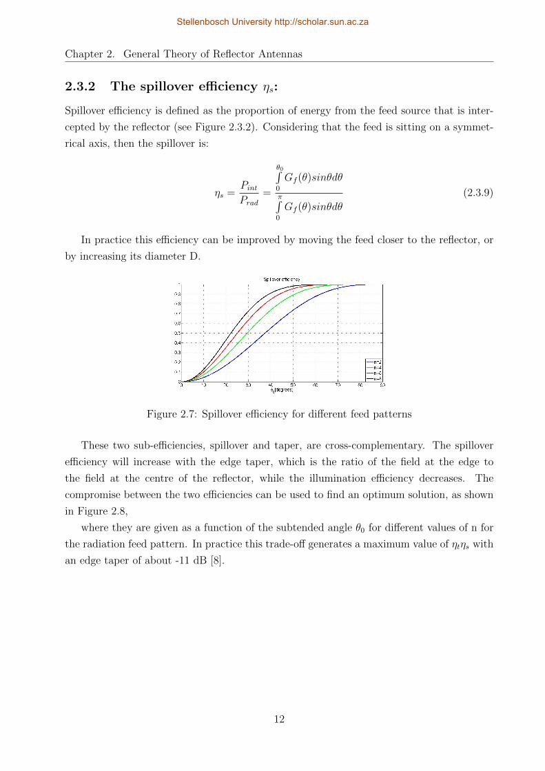
2.3.2 The spillover efficiency ηs:
Spillover efficiency is defined as the proportion of energy from the feed source that is inter-
cepted by the reflector (see Figure 2.3.2). Considering that the feed is sitting on a symmet-
rical axis, then the spillover is:
ηs =PintPrad
=
θ0∫0
Gf (θ)sinθdθ
π∫0
Gf (θ)sinθdθ
(2.3.9)
In practice this efficiency can be improved by moving the feed closer to the reflector, or
by increasing its diameter D.
Figure 2.7: Spillover efficiency for different feed patterns
These two sub-efficiencies, spillover and taper, are cross-complementary. The spillover
efficiency will increase with the edge taper, which is the ratio of the field at the edge to
the field at the centre of the reflector, while the illumination efficiency decreases. The
compromise between the two efficiencies can be used to find an optimum solution, as shown
in Figure 2.8,
where they are given as a function of the subtended angle θ0 for different values of n for
the radiation feed pattern. In practice this trade-off generates a maximum value of ηtηs with
an edge taper of about -11 dB [8].
12
Stellenbosch University http://scholar.sun.ac.za

Chapter 2. General Theory of Reflector Antennas
Figure 2.8: Trade-off between spillover and taper efficiencies
2.3.3 The polarization efficiency ηpol:
Polarization of an antenna is defined as the position and the direction of the electric field
with reference typically to the ground or surface of the earth. Depending on the orientation
of the electric and the magnetic fields, the polarization can be classified as linear, circular or
elliptical. Linear and circular polarization are special cases of elliptical polarization, when
the ellipse becomes a straight line or circle, respectively. For linear polarization, if the field
is oriented parallel to the ground, the polarization is called horizontal and the polarization is
known as vertical when the electric field is perpendicular to the ground. For the circular case,
the clockwise rotation of the electric field vector is designated as right-handed polarization
(RH) and left-handed polarization (LH) is the counter-clockwise, for an observer looking in
the direction of propagation [13],[14].
The polarization efficiency is the ratio of the power in the desired polarization Pco to the
total power intercepted by the reflector. It is affected by the polarization losses and can
be computed through the co and cross-polarization radiation patterns. Three definitions
of cross-polarization are explained by Ludwig in the literature [15]. However, analysis of
reflector antennas and feeds commonly use his third definition.
ηpol =PcoPrad
=
θ0∫0
|Cp (θ)|2 sinθdθ
θ0∫0
[|Cp(θ)|2 + |Xp (θ)|2
]sinθdθ
(2.3.10)
where Cp(θ) is the co-polarization, and Xp(θ) is cross-polarization.
2.3.4 The phase efficiency ηφ:
The phase efficiency represents the uniformity at the phase of the field across the aperture
plane. It depends on the relative position of the feed to the focal point of the reflector. Phase
13
Stellenbosch University http://scholar.sun.ac.za

Chapter 2. General Theory of Reflector Antennas
efficiency affects the gain and side lobes, and it can be computed in terms of the co-polarized
fields as [11]:
ηφ =
∣∣∣∣θ0∫0
Cp(θ)tan( θ2)dθ
∣∣∣∣2[θ0∫0
|Cp(θ)| tan( θ2)dθ
]2 (2.3.11)
2.3.5 The surface error efficiency ηr:
ηr is independent of the feeds illumination. It is associated with far-field cancellations arising
from phase errors in the aperture field caused by errors in the reflector’s surface. If δp is
the root mean square error(rms) on the surface of the reflector, the surface-error efficiency
is given by [16][8]:
ηr = e
−4πδpλ
2
(2.3.12)
2.4 Summary
The design of a reflector antenna should start with typical elementary steps such as:
Choose the size of the reflector based on the absolute gain or beamwidth requirements
against the cost and physical limitations such as weight.
Select a symmetric or offset configuration by considering the complexity against the
performance advantage of the offset design.
The efficiency should then be optimized by selecting a suitable feed to illuminate the
dish and by the choice of edge taper where one varies the reflector parameters, such as
the focal length to best suit the available feed.
In the case of a dual reflector, the aperture distribution can be further be controlled
by shaping the paraboloid and the sub-reflector. Shaped reflectors allow the aperture
efficiency to be enhanced over a parabolic reflector by using a ray-optical approach to
spread or concentrate the aperture energy needed.
14
Stellenbosch University http://scholar.sun.ac.za
Chapter 3
High-frequency Methods for Reflector
Antennas
Introduction
Dual reflector antennas are structurally and practically difficult to deal with because
of the number of geometrical parameters. However, they still have large areas of
application when high gain is desired. Several methods are available for the analysis of their
characteristics, which will depend upon the desired results, i.e, the methods applied depend
upon the size or the working frequency of the antenna. Recent computer development has
made computer-aided design the usual practice for the investigation of antenna properties.
This chapter highlights the high-frequency methods for the calculation of antenna patterns.
These methods are generally used for antenna structures much larger than a wavelength.
High frequency methods can be divided into two parts. Geometrical Optics, based on field
distribution is described in section 3.2 and section 3.3 highlighted Physical Optics described,
which is based on the current distribution. Both methods are limited by the diffraction
effects which occur on the aperture edges of the reflector. This phenomenon can be analysed
using the Geometrical Theory of Diffraction or the Physical Theory of Diffraction. Including
these effects for the analysis, then section 3.4.2 and 3.4.3 respectively describe the extension
of these 2 high-frequency techniques. Section 5 highlights the comparison between these two
techniques in the Plane Wave Spectrum method, based on the Fast Fourier Transform.
3.1 Radiation structures
A voltage connected to a radiating feed source creates a surface current density. This current
density creates an electromagnetic wave, which radiates into free space in the case of a
transmitter. For a reflector antenna, this radiation might also originate from the aperture
15
Stellenbosch University http://scholar.sun.ac.za

Chapter 3. High-frequency Methods for Reflector Antennas
plane of the paraboloid.
3.1.1 Radiation current source
The electromagnetic radiation is predicted by Maxwell’s equations for harmonic time-varying
fields. These following equations are the solutions represented in differential form and ap-
plying the Stockes’ theorem [17][18].
∇× E = −Jm − jwB (3.1.1)
∇×H = J + jwD (3.1.2)
∇ ·B = ρm (3.1.3)
∇ ·D = ρ (3.1.4)
E and H are the vector electric and magnetic field intensities. B is the magnetic flux
density and D represents the electric flux density.
Equations (3.1.1) and (3.1.2) are the Maxwell’s equations derived from Faraday’s and
Ampere’s Law respectively. Jm and J are the magnetic and electric conduction current
densities respectively, the angular frequency with w = 2πf . ρm is a fictitious magnetic
charge density and ρ is the electric charge density.
The radiation electric field away from the source can be computed over the current
distribution on the surface. This concept helps in the calculation of the electric or magnetic
field using E = −∇V . It is convenient also to define an electric or magnetic potential vector
to compute the magnetic or electric fields respectively. The differential equations for each
vector can be written as [16]:
A =µ
4π
∫V
Jese−jkR
Rds
′(3.1.5a)
Am =ε
4π
∫V
Jmse−jkR
Rds
′(3.1.5b)
where A and Am are, respectively, the electric and magnetic vector potentials , Jes and
Jms are the electric and magnetic current densities and the volume at which charge and
16
Stellenbosch University http://scholar.sun.ac.za
Chapter 3. High-frequency Methods for Reflector Antennas
current densities are nonzero. k is the wave number which is related to the wavelength λ.
k =2π
λ= w√µε (3.1.6)
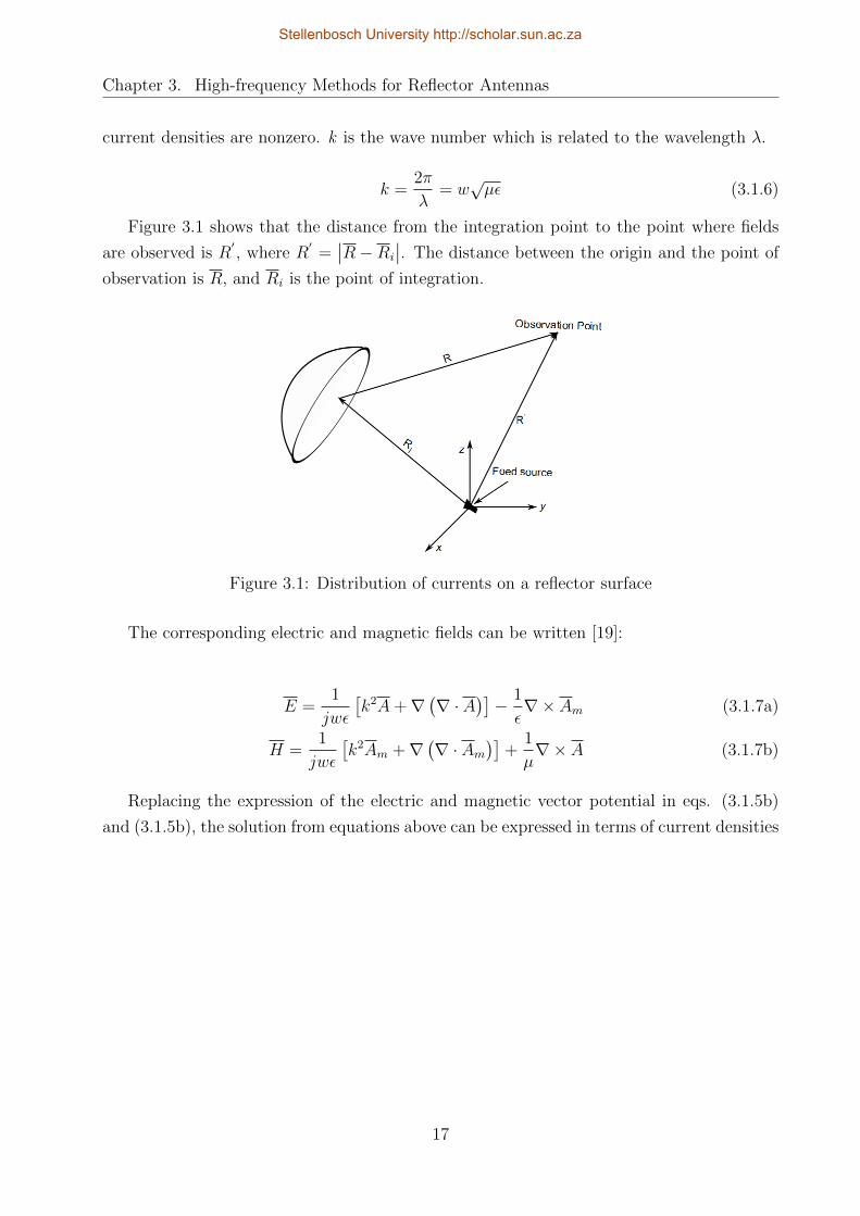
Figure 3.1 shows that the distance from the integration point to the point where fields
are observed is R′, where R
′=∣∣R−Ri
∣∣. The distance between the origin and the point of
observation is R, and Ri is the point of integration.
Figure 3.1: Distribution of currents on a reflector surface
The corresponding electric and magnetic fields can be written [19]:
E =1
jwε
[k2A+∇
(∇ · A
)]− 1
ε∇× Am (3.1.7a)
H =1
jwε
[k2Am +∇
(∇ · Am
)]+
1
µ∇× A (3.1.7b)
Replacing the expression of the electric and magnetic vector potential in eqs. (3.1.5b)
and (3.1.5b), the solution from equations above can be expressed in terms of current densities
17
Stellenbosch University http://scholar.sun.ac.za

Chapter 3. High-frequency Methods for Reflector Antennas
in the far and near fields:
E(R′) = − k
2
4π
∫V
[Jms × R
( jkR
+1
k2R
)]e−jkRds
′+
k2η
4π
∫V
[Jes
(− 1
kR− 1
k2R2+
j
k3R3
)+[Jes · R
]R( j
kR+
3
k2R2− 3j
k3R3
)]e−jkRds
′(3.1.8a)
H(R′) =
k2
4π
∫V
[Jes × R
( 1
kR+
1
k2R
)]e−jkRds
′+
k2
4πη
∫V
[Jms
(− 1
kR− 1
k2R2+
j
k3R3
)+[
Jms · R]R( j
kR+
3
k2R2− 3j
k3R3
)]e−jkRds
′(3.1.8b)
where,
R =R−Ri
|R−Ri|=R−Ri
R′ (3.1.9)
Only the terms with 1/R are taken into account in the far-field terms because at a
distance far from the source, terms in 1/R2 or 1/R3 will tend to zero. The radiative near-
field terms depend on 1/R2 terms, and near-fields terms have 1/R3 terms dependence. η is
the intrinsic (or wave) impedance (η = 377Ω in free space).
3.1.2 Aperture distribution source
Parabolic reflector antennas can be analysed as aperture antennas by assuming that their
surface is infinitely flat. The radiation far field can be computed from the electric and
magnetic fields over the aperture. The closed reflecting surface is divided by the aperture
plane into two spaces, as depicted in Figure 3.2; the one containing the source is called the
half-space and the second part is the free-source, where the radiation is calculated [20].
18
Stellenbosch University http://scholar.sun.ac.za

Chapter 3. High-frequency Methods for Reflector Antennas
Figure 3.2: Radiation fields on a reflector aperture plane
Huygen’s principle, as discussed in [10][16][21],is applied to calculate the radiation fields
on the aperture plane,viz, the incident field in the aperture is replaced by an equivalent
magnetic and electric source on a closed surface and this equivalent source is assumed to be
zero outside the surface. This new current source can be expressed mathematically as:
Jes = n×H = n× (H2 −H1) (3.1.10a)
Jms = −n× E = −n× (E2 − E1) (3.1.10b)
where H1 and E1 represent the tangential magnetic and electric fields on the first region
(region 1); H2 and E2 are fields on region 2 and n is the unit vector normal to the surface.
The parabola surface is assumed to be an infinite plane, and if fields (E,H) on the first
region are chosen to be zero, then, currents in (3.1.10a) and (3.1.10b) are calculated on the
boundary and can be expressed in term of the aperture magnetic and electric field as:
Jes = n×Ha (3.1.11a)
Jms = −n× Ea (3.1.11b)
The radiation pattern of reflector antennas can either be computed from the distribution
of surface currents on the reflectors, or from the prime reflector aperture field, by considering
the reflector antenna as an aperture radiator. These methods are called, respectively, the
current distribution method and the aperture distribution method. These methods are
specified as an asymptotic high frequency method and ignore the diffraction effects on the
reflector surface.
19
Stellenbosch University http://scholar.sun.ac.za
Chapter 3. High-frequency Methods for Reflector Antennas
3.2 Geometric Optics theory
Geometrical optics or the ray optics technique is based on the aperture distribution assump-
tion, to compute the propagation wave for the incident, reflected and the refracted fields.
Maxwell’s equation’s prediction of the electromagnetic wave is related to the Geometrical
Optics as discussed in [22]. The GO method is accurate for analysing or designing reflec-
tor antennas, since they have large dimensions compared to the wavelength. Then, too, its
approximation cost is independent of the size of the structure and its accuracy improves as
structure size increases.
The classical geometrical optics starts from Fermat’s principle. Fermat’s principle states
that the path of a light ray follows is an extremum in comparison with the nearby paths.
The optical path length is defined as [23]:
δ
∫ P1
P0
n(s)ds (3.2.1)
where P0 and P1 are the extremum, δ represents the calculus variation and n(s) is the index
of refraction of the medium, which is a function of position along the path between points P0
and P1. In a homogeneous medium, the rays are straight lines wherein the index of refraction
is constant.
n(s) =
√µε
µ0ε0(3.2.2)
The solution of the electric and magnetic fields from the exact electromagnetic theory
can be expanded into power series in inverse powers of the angular frequency ω [24][25].
E(R′, ω) = e−jk0L(R
′)
∞∑m=0
Em(R′)
(jω)m(3.2.3a)
H(R′, ω) = e−jk0L(R
′)
∞∑m=0
Hm(R′)
(jω)m(3.2.3b)
where L(R′) is called the optical path length or eikonal and k0 =
√µ0ε0 is the propagation
constant in the vacuum. The equiphase wave fronts are given by the level surfaces of the
eikonal function. The polarisation, the phase and wavelength are not taken into account
in the classical geometric optics. The extension of this technique can be done by using the
asymptotic solution of the Maxwell’s equation as ω →∞.
E(R′, ω) ≈ E0(R
′)e−jk0L(R
′) (3.2.4a)
H(R′, ω) ≈ H0(R
′)e−jk0L(R
′) (3.2.4b)
20
Stellenbosch University http://scholar.sun.ac.za
Chapter 3. High-frequency Methods for Reflector Antennas
In geometric optics, the eikonal equation came from the solution of the Maxwell’s equa-
tion, which is expressed in form [23]:
∣∣∇L(R′)∣∣2 = n2 (3.2.5)
where the function L(R′) must satisfy the differential equation:
|∇L|2 =
(∂L
∂x
)2
+
(∂L
∂y
)2
+
(∂L
∂z
)2
= n2 (3.2.6)
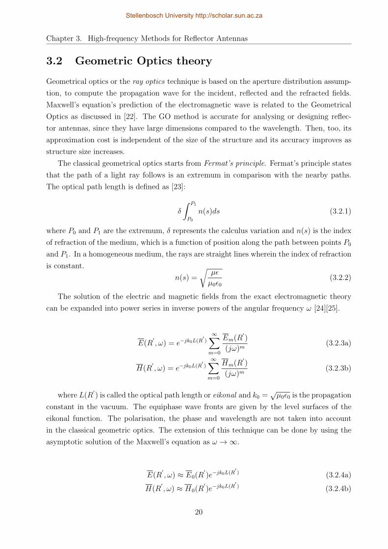
3.2.1 Propagation of rays in Geometrical Optics
The principle of GO can be proved by computing a secondary wave front surface Ln after a
short time t = tn+1 > tn with (n = 0, 1, 2, · · · ), from a primary wave front surface L0 at t0,
as illustrated in Figure 3.3. This secondary wave front is a straight line for an homogeneous
medium. However, it has a curvature in an inhomogeneous medium.
Figure 3.3: Primary and secondary wave of radiated wave after [24].
Since the rays in the medium move in a velocity equal to the velocity of light, the phase
increases between the 2 successive surfaces (ω/c)δL, while the wave traverses from one surface
to another with a time difference δt = t1−t0. Then, the secondary wave front L1 is described
from the connection of the surface normal to each of the rays [24].
The wave fronts are defined by letting the function L(R′) equal a constant. The local
wave vector ∇L(R′) evaluated at any point in space is always normal to the wave front
passing through it. The direction of the ray can be expressed as [26].
s =∇Ln
(3.2.7)
21
Stellenbosch University http://scholar.sun.ac.za

Chapter 3. High-frequency Methods for Reflector Antennas
where s is the unit vector normal to the wave front. The fields at any point over a ray
are perpendicular to the ray.
3.2.2 Reflection on the boundary
To enhance the use of geometric optics, it is more important to define the behaviour of
the ray on the boundary, rather than determining the geometrical optics properties of rays
through the surface. In geometrical optics, the direction of the fields is defined by the ray
equation. Let r(s) be the position vector of the ray over the path and, since s = dr/ds, the
equation can be written from (3.2.7) as [26]:
d2r
ds2=dr
ds· ∇(dr
ds
)= s · ∇(s) =
∇Ln· ∇(∇Ln
)(3.2.8)
In an homogeneous medium this equation is equal to zero, at which the wave front is a
straight line.
d2r
ds2=
1
2∇(|∇L|2
n2
)= 0 (3.2.9)
At the boundaries, as the 2 mediums differ from each other in their reflective indexes
respectively, n1 and n2, as illustrated in Figure 3.4, the behaviour of the ray follows Snell’s
Law. The equation (3.2.8) is integrated at the point of reflection, where the tangential
component of the rays is vanishing, thus the incident ray is related to the reflected. Applying
Stoke’s theorem and assuming that the boundary surface is for δ → 0.∫∫dS · ∇ × (sn) =
∮C
dl · sn = 0 (3.2.10)
where dl is the differential line over the closed reflection surface and dS is the unit vector
normal to the surface.
Figure 3.4: Derivation from Snell’s Law: the unit vector si is in the direction of the incidentray and sr is in the direction of the reflected ray after [24]
22
Stellenbosch University http://scholar.sun.ac.za

Chapter 3. High-frequency Methods for Reflector Antennas
From Snell’s principle, the transmitted and reflected ray are:
n1sinθi = n2sinθt (3.2.11)
and at the reflection region, the indexes of refraction are identical (n1 = n2). From Figure
3.4, the angle of reflection is θt + θr = π. Therefore the relation between the incident and
reflected angles is:
n1sinθi = n1sinθr (3.2.12)
3.2.3 Propagation power of the rays
In geometric optics, the power per unit solid angle between two points is influenced by the
conservation of energy flux in a tube of rays [24]. The total power within the cross section
of the flux tube must be constant since power propagates in the direction of the rays only.
When the flux tube cross section dA0 and power density S0 are known at a reference point
and the flux tube cross section area dA is known, then the radiation density S is given in
terms of S0 as:
S0dA0 = SdA (3.2.13)
Radiation densities S and S0 are assumed constant throughout the cross section areas
dA0 and dA respectively, thus no power flows across the side of the tube [8]. For the
electromagnetic wave, the time average Poynting vector can be written as [26]:
S =1
2ReE ×H∗ =
1
2nηReE ×
(∇L× E
)∗=
1
2nη
(E · E
)∗∇L= s
1
2η
∣∣E∣∣2 (3.2.14)
3.3 Physical Optics theory
Physical Optics (PO) or wave optics is one of the high frequency methods commonly used
for reflector antenna analysis because of its accuracy. It is based on current distribution
method by using Huygen’s principle as discussed in §3.1.1.
23
Stellenbosch University http://scholar.sun.ac.za

Chapter 3. High-frequency Methods for Reflector Antennas
3.3.1 Induced current density for PEC
The principle of PO is to integrate the induced current distribution on the reflector surface.
Considering the surface as a perfect conductor, the induced current density is the compo-
sition of the incident and reflected tangential magnetic fields on the surface. Ignoring the
contribution of current on the reflector shadowed region and the tangential component, the
H -field on the surface is doubled on the illuminated region, according to the method of im-
ages [27][24]. Assuming the reflecting surface to be locally plane, the physical optics current
density for a PEC (n×H i= n×Hr
) is given by:
Js =
n×
(Hi+H
r); illuminated region
0 ; shadowed region(3.3.1)
or
Js =
2n×H i
; illuminated region
0 ; shadowed region(3.3.2)
where Hi
and Hr
are the incident and reflected magnetic fields computed across the surface.
In case of a dual reflector , the radiation field may radiate from the feed source or be
scattered from the sub-reflector. The PO technique can account for diffraction, interference
and polarization effects, as well as aberrations and other complex effects.
The radiation current density approximation represented in (3.3.2) is defined as the
Physical Optics approximation. It is valid only for large electrical size antenna structures,
i.e. either the radius of curvature of the reflector or the radius of curvature of the incident
wave are greater than about 5λ [27][28].
3.3.2 PO radiation fields
The radiation fields scattered on the reflector surface can be computed using eqs. (3.1.8a)
and (3.1.8b). The PO current over the surface is assumed to be constant in amplitude and
phase, the radiation integral is then reduced to a simple summation [16]. From (3.1.8b), the
magnitude of the magnetic field over a conducting surface is:
H(Ri) = − 1
4π
∫∑(jk +
1
R′
)R× Js(Ri)
e−jkR′
R′ ds (3.3.3)
Computation is simplified by replacing the reflector surface∑
by an adjacent N -plane
rectangular facet ∆k, where k = 1, · · · , N corresponds with the triangle. Replacing the
24
Stellenbosch University http://scholar.sun.ac.za
Chapter 3. High-frequency Methods for Reflector Antennas
surface∑
by the triangle facet, then (3.3.3) becomes [29]:
H(Ri) = − 1
4π
N∑k=1
(jk +
1
R′k
)Rk × Tk(Ri)ds (3.3.4)
in which,
Tk(Ri) =
∫∆k
Jk(Ri)e−jkR
′
R′ ds (3.3.5)
and the PO surface current on the surface can be expressed in terms of the incident field
Hs.
Jk(Ri) = 2nk ×Hs(Ri) (3.3.6)
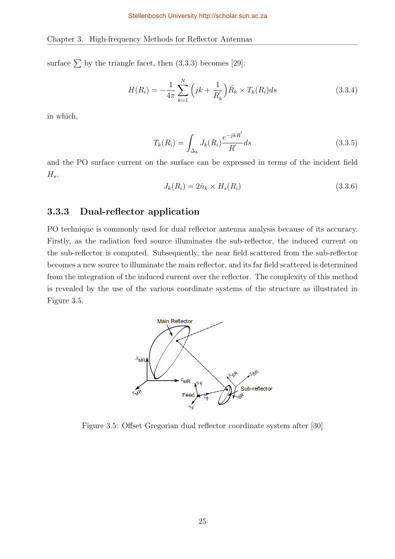
3.3.3 Dual-reflector application
PO technique is commonly used for dual reflector antenna analysis because of its accuracy.
Firstly, as the radiation feed source illuminates the sub-reflector, the induced current on
the sub-reflector is computed. Subsequently, the near field scattered from the sub-reflector
becomes a new source to illuminate the main reflector, and its far field scattered is determined
from the integration of the induced current over the reflector. The complexity of this method
is revealed by the use of the various coordinate systems of the structure as illustrated in
Figure 3.5.
Figure 3.5: Offset Gregorian dual reflector coordinate system after [30]
25
Stellenbosch University http://scholar.sun.ac.za

Chapter 3. High-frequency Methods for Reflector Antennas
3.4 Analysis of the diffraction effect on the sub-reflector
rim
3.4.1 Huygens-Fresnel principle of diffraction
One of the most difficult problems to solve in optics is the diffraction phenomenon. Diffrac-
tion theory is based on the Huygens-Fresnel principle. According to Huygens’ construction,
every point on a primary wave-front serves as a source of secondary spherical wavelets, such
that the primary wave-front is the envelope of these wavelets in a subsequent time (see Fig-
ure 3.6). Moreover, the wavelets advance with a speed and frequency equal to those of the
primary wave at each point in space. This principle was further added to Fresnel, where the
superposition of the secondary wave-front takes into account the amplitude and phase of the
wavelets [31].
Figure 3.6: Huygens geometry construction
The GO described earlier is used to determine the scattering field in the illuminated region
but cannot predict the non-zero field in the shadow. However, the analysis of diffraction on
the parabolic reflector edges or rim will permit the computation of the field in the shadow
region as illustrated in Figure 3.7. Wave diffraction in space is a local phenomenon at high
frequency, hence the field value of the diffracted rays is proportional to the field value of
the incident rays at the point of diffraction multiplied by a coefficient called the diffraction
coefficient [8].
26
Stellenbosch University http://scholar.sun.ac.za

Chapter 3. High-frequency Methods for Reflector Antennas
Figure 3.7: Rays diffracted in the parabolic reflector edges [32][23].
where QE is the diffraction point, the incident rays to the edge forms the edge diffracted
field ed ans the surface diffracted field sr. ES is the boundary between between ed ans sr
and tangent to the surface on QE. RB and SB define the shadow boundaries of the incident
and reflected field, respectively.
The computation of this diffraction coefficient depends strictly on the properties of the
waves and the boundary where the point of diffraction is considered. The complex geometries
of reflector antennas are approximated with the help of canonical problems to investigate
the diffracted field, where the exact edge geometry is simplified by this canonical problem.
This simple model is then used to calculate the diffracted field. The surface edge geometry
is defined for a canonical problem and the examination is reduced into a half plane problem
for analysis of a cylindrical reflector antenna.
3.4.1.1 Edge diffraction in the sub-reflector surface
The electromagnetic wave from the feed source illuminates the ellipsoid sub-reflector surface,
and the total electric field Etot is the sum of the incident field from the source Ei and the
radiated field from the reflector Er for a finite size antenna. However, in a discontinuous
medium such as an edge, the field on the shadowed region is not negligible according to
Huygens source. The total field in the aperture is given for this case as [23]:
−→E tot =
−→E iui +
−→E rur +
−→E d (3.4.1)
where−→E d is the edge diffracted field. The GO method can evaluate directly
−→E i and
−→E r;
and the diffraction integral is applied for−→E d resolution.
The analysis of reflector antennas results in a great improvement performance when
accounting the diffraction on the edge. The following sections describe the extension of the
27
Stellenbosch University http://scholar.sun.ac.za

Chapter 3. High-frequency Methods for Reflector Antennas
PO and GO methods, respectively called PTD or Physical Theory of Diffraction and GTD
or Geometric Theory of Diffraction.
3.4.2 Geometrical Theory of Diffraction
An incoming incident rays striking an edge surface boundary creates non-uniform diffracted
rays. Either PTD or GTD are, respectively, techniques used to describe this diffraction
phenomena at a particular region called the shadow, wherein, the electric field is assumed
to be zero for the ordinary GO.
3.4.2.1 Geometrical Optics fields
The GTD presented in this section is an assumption technique developed by Keller in 1950s
for the extension of GO as described in [33]. To make use of the efficiency of GO, Keller
took into account the diffracted ray in the shadow region; however the GTD is still limited
because of the non-uniformity of the diffracted fields on the transition region surrounding the
surface boundary [34]. Keller’s conception is based on Fermat’s principle, and investigates
the diffraction point location and the orientation of the diffracted rays propagation.
3.4.2.2 Diffracted fields on a curved surface
Figure 3.8 represents the diffraction at the curved surface edge. For an oblique incident ray
having an angle β0 on the edge, the diffracted field lies on the surface of a cone with an angle
β0/2. The diffracted electric field on the surface is expressed as [23]:
Ed(s) = Ei(QE) ·D(φ, φ′, β0)A(s)e(−jks) (3.4.2)
where Ei(QE) is the incident field at the point of diffraction QE, D(φ, φ′, β0) is the dyadic
diffraction coefficient for a perfect conducting wedge.
28
Stellenbosch University http://scholar.sun.ac.za

Chapter 3. High-frequency Methods for Reflector Antennas
Figure 3.8: Diffracted at a curved edge [24].
Then, the spacial attenuation factor or spreading factor A(s), which is defined as the
variation of the field intensity along the diffracted ray, for an incident spherical wave is given
as [24]:
A(s) =
√ρ
s(ρ+ s)≈√ρ
sfor s ρ (3.4.3)
where s is the distance from the diffraction point to the field observation point and the ρ
is the distance between the caustic at the edge and the second caustic of the diffracted ray.
The caustic distance ρ is related to the normal incidence β′0 as [35]:
1
ρ=
1
ρe− ne · (s
′ − s)asin2β0
(3.4.4)
in which,
ρe is the radius of curvature of the incident wave front at the point of diffraction taken into
the plane of the incident ray, containing the unit vectors s′
and e;
a is the radius of curvature of the edge at the point of diffraction QE, and
ne is the unit normal vector to the edge directed away from the centre of curvature.
From Figure 3.8, the unit vectors β0
′
and β0 are related respectively by:
β0
′
= s′ × φ′
(3.4.5a)
β0 = s× φ (3.4.5b)
29
Stellenbosch University http://scholar.sun.ac.za

Chapter 3. High-frequency Methods for Reflector Antennas
The diffracted field is obtained from the dyadic diffraction coefficient at the edge. This
diffraction coefficient can be described by:
D(φ, φ′; β0) = −β ′
0β0Ds(φ, φ′; β0)− φ′
φDh(φ, φ′, β0) (3.4.6)
where Ds and Dh are, respectively, the scalar diffraction coefficient for the soft boundary
condition (Dirichlet) and the scalar diffraction coefficient for the hard (Neumann) boundary
condition at the edge. They can be represented respectively by:
Ds(φ, φ′; β0) = Di(φ, φ
′; β0)−Dr(φ, φ
′; β0), (3.4.7a)
Dh(φ, φ′; β0) = Di(φ, φ
′; β0) +Dr(φ, φ
′; β0) (3.4.7b)
where
Di,r(φ, φ′; β0) = − e−jπ/4
2n√
2πβsinβ′0
×
cot[π + (φ+ φ
′)
2n
]F [kLia+(φ− φ′
)]
+cot[π − (φ− φ′
)
2n
]F [kLia−(φ− φ′
)]
∓cot[π + (φ+ φ
′)
2n
]F [kLrna+(φ− φ′
)]
+cot[π + (φ+ φ
′)
2n
]F [kLroa−(φ+ φ
′)]
(3.4.8)
wherein F (X) is the transition function expressed as:
F (X) = 2j√XejX
∫ ∞√X
e−jτ2
dτ ; (3.4.9)
and
a±(φ± φ′) = 2cos2
(2nπN± − (φ± φ′
)
2
)(3.4.10)
at which N± are the integers which mostly satisfy the equations [23]:
2πnN+ − (φ± φ′) = π (3.4.11a)
2πnN− − (φ± φ′) = −π (3.4.11b)
30
Stellenbosch University http://scholar.sun.ac.za
Chapter 3. High-frequency Methods for Reflector Antennas
where Li and Lr are the distance parameters, which expressed as
Li =s (ρie + s) ρi1ρ
i2β0
ρie (ρi1 + s) (ρi2 + s); (3.4.12a)
Lr =s (ρr + s) ρr1ρ
r2β0
ρr (ρr1 + s) (ρr2 + s)(3.4.12b)
where ρi1, ρi2 and ρr1, ρr2 are the principal radii of curvature of the incident wavefront and
the reflected wavefront at the point of diffraction QE respectively. Then, ρie, ρir are radii
of curvature of the incident and reflected wave front at the point QE taken from the plane
containing the incident, the reflected and diffracted ray respectively and the unit vector e.
The superscripts ”o” and ”n” on Lr in equation (3.4.8) indicate the radii of curvature ρr1,
ρr2 and the distance parameters ρr must be calculated from the ”o” face and ”n” face of
the wedge. At the far field observation where s ρi, ρi1, ρi2, ρ
r, ρr1, ρr2, eqs. (3.4.12a) and
(3.4.12b) reduce into:
Li =ρi1ρ
i2
ρiesin2β
′
0 (3.4.13)
and
Lro = Lrn = Lr =ρr1ρ
r2
ρrsin2β
′
0 (3.4.14)
3.4.3 Physical Theory of Diffraction
The PTD or Physical Theory of Diffraction is an asymptotic technique developed in the
1950s by Professor Ufimtsev to overcome the diffraction issue [36]. It is an improvement of
PO technique wherein the diffraction effects such as the discontinuity of the surface currents
at boundaries of the illuminated and shadow regions near the edges of the surface is taken
into account.
The PO current in (3.3.2) §3.3.1 is corrected by a nonuniform current that accounts for
diffraction effects and is expressed as [37]:
−→J s(r) =
−→J PTD(r)−
−→J PO(r) (3.4.15)
where−→J PO(r),
−→J PTD(r) are the PO and the PTD current contribution respectively,
Js(r) is the surface current density.
Besides, the scattered field in PTD is, of course, different from that calculated using
the Geometrical Theory of Diffraction, because it includes the ”nonuniform” current or the
fringing current at the surface edges. The total scattered fields resulting from the current
31
Stellenbosch University http://scholar.sun.ac.za

Chapter 3. High-frequency Methods for Reflector Antennas
on the surface is given as:
Estot(r) = Es
PO(r) + EsPTD(r) (3.4.16)
EsPO(r) and Es
PTD(r) are the PO and the PTD scattered fields respectively. The compu-
tation of the scattered fields for this present method is discussed in the next paragraph.
3.4.3.1 Method of Equivalent Current
EsPTD(r), called the correction term, can be calculated by using the Method of Equivalent
Current(MEC). The MEC reduces the evaluation of surface integrals for the fringe surface
currents to line integrals around the edges of the surface of the scatterer, as discussed in
literature [38],[39]. Using MEC, the PTD scattered fields are described as:
EsPTD(r) =
jk0
4π
∮(η0r × r × If + s×Mf )
−jk0r
rdl (3.4.17)
If and Mf are the fringe electric and the magnetic equivalent edge currents respectively.
Asymptotic techniques as GTD and PTD have been performed to deal with the diffraction
problem. However, they are sometimes limited by the size and the complexity of the geometry
of the antenna, even though several approximations are applied to accomplish the task and
to obtain the correct results.
Actually, the development of various software solutions for antenna analysis not only
reduces the task of an engineer, but also standardises a low cost antenna design. Moreover,
the electromagnetic problem involving particularly the scattering, propagation, radiation
and acoustic fields can be also proved using a Plane Wave Spectrum or PWS. This method
is outlined in a subsequent section.
3.5 Antenna Radiation pattern using Plane Wave Spec-
trum
Several methods have been developed for the resolution of electromagnetic problems. Each
method has its own particular advantages. The combination of methods is actually necessary
to investigate the properties of antennas with complex geometry.
Superposition of plane waves propagating in different directions with different amplitudes
is called a Plane Wave Spectrum or an angular spectrum of a plane wave [1]. It is applied to
compute the test zone field from a known reflector aperture field distribution. This method is
accurate for the investigation of reflectors having a notched rim for reduced edge diffraction
[40].
32
Stellenbosch University http://scholar.sun.ac.za

Chapter 3. High-frequency Methods for Reflector Antennas
3.5.1 Plane waves spectrum representation
The properties of a plane wave travelling in a uniform, isotropic and lossless open region is
described in literature [41]. Waves are said to be plane if their equi-phase surface is planar.
If the equiamplitude surfaces of plane waves are also equiphases, then, they are known as
homogeneous. Assuming that the total field satisfies the harmonic time dependence ejwt,
given by the homogeneous Helmholtz equation [19] [42]:
∇2E(x, y, z) + k0E(x, y, z) = 0 (3.5.1)
where k0 = w√µ0ε0 is the wave number in free space. Therefore, the electric field solution
of (3.5.1) can be written in terms of the angular spectrum, which is the superposition of
plane waves propagating in different directions with different amplitudes:
E(x, y, z) =1
4π2
∫ +∞
−∞
∫ +∞
−∞F (kx, ky, z)e
−jkrdkxdky (3.5.2)
Figure 3.9 illustrated the free space propagator vector k and the position vector r are re-
spectively and they are described by:
k = kxx+ kyy + kz z = k0(ux+ vy + wz) (3.5.3a)
r = xx+ yy + zz (3.5.3b)
In spherical coordinates, u = sinθcosφ, v = sinθsinφ and w = cosθ are the direction
cosine.
Figure 3.9: Plane wave propagation coordinate system.
By replacing the value of k and r, (3.5.2) can be written in spectral domain for z = 0 as
[43][44]:
E(x, y, 0) =1
4π2
∫ ∞−∞
∫ ∞−∞
F (kx, ky)e−j(kxx+kyy)dkxdky (3.5.4)
33
Stellenbosch University http://scholar.sun.ac.za

Chapter 3. High-frequency Methods for Reflector Antennas
and the wave number in z-direction is given by:
k2z = k2
0 −(k2x + k2
y
)(3.5.5)
or
kz =
+√k2
0 − (k2x + k2
y), if k2x + k2
y ≤ k20
−j√
(k2x + k2
y)− k20, if k2
x + k2y > k2
0
(3.5.6)
when k2x + k2
y ≤ k20, the real value of kz will correspond with the radiation field of the
aperture, kz corresponds to the evanescent waves for k2x + k2
y > k20, and F (kx, ky) is the
two-dimensional angular spectrum of the field.
3.5.2 The Angular spectrum approximation
The antenna far field is approximated by the angular spectrum. The PWS method requires
two general assumptions for far field antenna computation which are [1]:
a. the aperture antenna dimensions have a finite length, wherein the field sources lying
in the half-space behind the aperture plane are finite and occupy a finite volume;
b. the kr values must be large compared to the wavelength and the greatest dimension
of the aperture .
The two-dimensional inverse Fourier transform integral is computed using the method of
stationary phase, as described in literature [41][6]. The integral equation (3.5.6) is computed
using this method and the radiated far field can be expressed approximately as:
E(r, θ, φ) ' jkejkr
2πr[cosθf(kx, ky)] (3.5.7)
with
f(kx, ky) = fx(kx, ky)x+ fy(kx, ky)y + fz(kx, ky)z (3.5.8)
The θ and φ components are dominant in the far zone field. (3.5.7) shows that the two-
dimension inverse Fourier transform can be approximated into a multiplication of a normali-
sation constant with a trigonometric function. Despite this fact (3.5.7) is valid for only some
values of stationary points which can be described as:
kx = k0sinθcosφ (3.5.9a)
ky = k0sinθsinφ (3.5.9b)
kz = k0cosθ (3.5.9c)
34
Stellenbosch University http://scholar.sun.ac.za

Chapter 3. High-frequency Methods for Reflector Antennas
The Eθ and Eφ component can then be written as:
Eθ(r, θ, φ) ' jkejkr
2πr(fxcosθ + fysinφ) (3.5.10a)
Eφ(r, θ, φ) ' jkejkr
2πr(−fxsinθ + fycosφ) (3.5.10b)
3.6 Conclusion
In this chapter a brief overview of some high frequency asymptotic techniques from CEM
theory are presented. It is shown that the diffraction limitations of the GO and PO tech-
niques can be corrected for by including the diffraction term analysis using the PTD and
GTD extension methods. These are based on the physical and geometrical assumption re-
spectively and are accurate for electrically large antennas. These two techniques used often
for computer-aided applications because they produce favourable memory and runtime re-
sults. Even if several approximations are assumed for the dual reflector antenna analysis,
these high-technique methods are restricted by the complexity of the dual reflector antenna
geometry.
35
Stellenbosch University http://scholar.sun.ac.za
Chapter 4
Description of a Gregorian Reflector
Antenna and Creation of a FEKO
Reference
Introduction
Areflector antenna with a low polarization and side lobe level is difficult to engineer
because of the aperture blockage or scattering of the feed or sub-reflector. An offset
antenna is a most interesting structure employed to avoid not only this blockage, but also the
multiple reflections between the feed and reflectors, although an increase of cross polarization
is the penalty.
This chapter highlights a description of a classical offset dual reflector; section 4.1 shows
the geometry structure for a particular type of offset reflector, section 4.1.5 describes pa-
rameters of the design and section 4.2.1 investigates the feed system.
The full antenna radiation properties are computed using a numerical method, based on a
combination of Method of Moments (MoM) and the Physical Optics high frequency technique
using a software package FEKO in section 4.2. This technique is suitable for accurate analysis
of an offset dual reflector antenna when the following is done: an analytical function is used
to approximate the pattern of the feed, and the antenna system is then subdivided into two
parts with ; the MoM applied for the small sub-reflector and PO for the main reflector.
36
Stellenbosch University http://scholar.sun.ac.za

Chapter 4. Description of a Gregorian Reflector Antenna and Creation of a FEKOReference
4.1 Description of the Gregorian Reflector Antenna
4.1.1 Gregorian geometry structure
An offset Gregorian reflector antenna is a paraboloidal reflector with a concave sub-reflector
of ellipsoidal shape, located at a distance from the vertex of the prime reflector, that dis-
tance being greater than the prime focal distance of the main reflector. The system offers
several significant advantages over its axis-symmetric counterpart for many applications,
such as remote sensing, satellite communications, radio astronomy, etc. Figure 4.1 depicts
the geometric structure of this antenna and its parameters are described in Table 4.1.
Figure 4.1: Front and side view of a Gregorian dual reflector after [45]
F0 and F1 are the foci of the ellipsoid sub-reflector. F0 is pointed at the prime reflector
focal point and the feed source is placed at F1. Rays from F1 are reflected by the sub-reflector.
Reflected rays will emanate the main reflector through F0.
(0, xsr, zsr) is the sub-reflector axis and (0, xm, zm) defines the main reflector axis, which
is situated at the system axis (0, x, z). These two axes are tilted at an angle β. Angles are
considered positive if the rotation on the y axis is counterclockwise, and negative if in the
opposite direction [46], except for the angle θe on the sub-reflector, which is always positive.
37
Stellenbosch University http://scholar.sun.ac.za
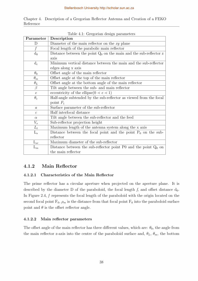
Chapter 4. Description of a Gregorian Reflector Antenna and Creation of a FEKOReference
Table 4.1: Gregorian design parametersParameter Description
D Diameter of the main reflector on the xy planef Focal length of the parabolic main reflectord0 Distance between the point Q0 on the main and the sub-reflector z
axisdc Minimum vertical distance between the main and the sub-reflector
edges along x axisθ0 Offset angle of the main reflectorθm Offset angle at the top of the main reflectorθL Offset angle at the bottom angle of the main reflectorβ Tilt angle between the sub- and main reflectore eccentricity of the ellipse(0 ≺ e ≺ 1)θe Half-angle subtended by the sub-reflector as viewed from the focal
point F1
a Surface parameter of the sub-reflectorc Half interfocal distanceα Tilt angle between the sub-reflector and the feedVs Sub-reflector projection heightLt Maximum length of the antenna system along the x axisLs Distance between the focal point and the point P0 on the sub-
reflectorLsr Maximum diameter of the sub-reflectorLm Distance between the sub-reflector point P0 and the point Q0 on
the main reflector
4.1.2 Main Reflector
4.1.2.1 Characteristics of the Main Reflector
The prime reflector has a circular aperture when projected on the aperture plane. It is
described by the diameter D of the paraboloid, the focal length f, and offset distance d0.
In Figure 2.4, f represents the focal length of the paraboloid with the origin located on the
second focal point F0, ρm is the distance from that focal point F0 into the paraboloid surface
point and θ is the offset reflector angle.
4.1.2.2 Main reflector parameters
The offset angle of the main reflector has three different values, which are: θ0, the angle from
the main reflector z-axis into the centre of the paraboloid surface and, θL, θm, the bottom
38
Stellenbosch University http://scholar.sun.ac.za
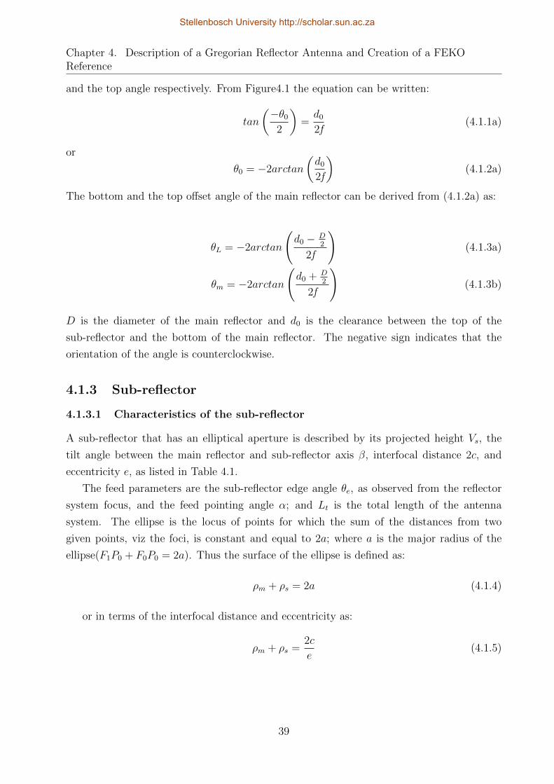
Chapter 4. Description of a Gregorian Reflector Antenna and Creation of a FEKOReference
and the top angle respectively. From Figure4.1 the equation can be written:
tan
(−θ0
2
)=d0
2f(4.1.1a)
or
θ0 = −2arctan
(d0
2f
)(4.1.2a)
The bottom and the top offset angle of the main reflector can be derived from (4.1.2a) as:
θL = −2arctan
(d0 − D
2
2f
)(4.1.3a)
θm = −2arctan
(d0 + D
2
2f
)(4.1.3b)
D is the diameter of the main reflector and d0 is the clearance between the top of the
sub-reflector and the bottom of the main reflector. The negative sign indicates that the
orientation of the angle is counterclockwise.
4.1.3 Sub-reflector
4.1.3.1 Characteristics of the sub-reflector
A sub-reflector that has an elliptical aperture is described by its projected height Vs, the
tilt angle between the main reflector and sub-reflector axis β, interfocal distance 2c, and
eccentricity e, as listed in Table 4.1.
The feed parameters are the sub-reflector edge angle θe, as observed from the reflector
system focus, and the feed pointing angle α; and Lt is the total length of the antenna
system. The ellipse is the locus of points for which the sum of the distances from two
given points, viz the foci, is constant and equal to 2a; where a is the major radius of the
ellipse(F1P0 + F0P0 = 2a). Thus the surface of the ellipse is defined as:
ρm + ρs = 2a (4.1.4)
or in terms of the interfocal distance and eccentricity as:
ρm + ρs =2c
e(4.1.5)
39
Stellenbosch University http://scholar.sun.ac.za

Chapter 4. Description of a Gregorian Reflector Antenna and Creation of a FEKOReference
4.1.3.2 Reflection from the sub-reflector
The ellipse is rotated about its axis to form solid a figure that reflect incident spherical waves
into spherical waves with different caustics (focus).The sub-reflector changes the curvature
of waves coming from one focus into waves with their caustic at the second sub-reflector
focus. In polar coordinates, this can be defined as:
ρ =eT
1− ecosθ(4.1.6)
where T is the distance from the focal point into a line called the directrix Figure 4.2(b)
[47], ρ is the distance from the focus onto the sub-reflector surface and θ is the offset main
reflector Figure 4.2(a).
(a) (b)
Figure 4.2: Ellipsoid geometry. (a) rectangular coordinate. (b)section of the ellipse sub-reflector
The eccentricity e of the sub-reflector is the ratio of the distance from the origin of a point
on the curve to the distance from the same point to the directrix e = R1
R2. For a Gregorian
system this distance T is given in terms of the interfocal distance as [16]:
T =c(1− e2)
e2(4.1.7)
Put (4.1.7) into (4.1.6), the distance from the left focus of the sub-reflector denoted ρm
is:
ρm =(ce
) e2 − 1
ecosγm − 1(4.1.8)
40
Stellenbosch University http://scholar.sun.ac.za

Chapter 4. Description of a Gregorian Reflector Antenna and Creation of a FEKOReference
and the distance from F0 onto the sub-reflector surface can be derived:
ρs = −(ce
) e2 − 1
ecosγs + 1(4.1.9)
The projection of the line F1P0 onto the sub-reflector axis zsr gives angle γm, and γs is
the projection of the line F0P0 onto the zsr axis. These angles are related by the eccentricity
[48].
(e+ 1)tan(γm
2
)= |e− 1| tan
(γs2
)(4.1.10)
4.1.4 Equivalent parabola analysis
A dual offset reflector model can be geometrically transformed on its equivalent parabola.
This new geometry is based on the optics theory and eases the analysis. This model geometry
is illustrated in Figure 4.3. An equivalent parabola geometry has the same diameter as the
dual offset (D = Deq), but its focal length feq is longer than that of the paraboloid main
reflector. The ratio of these 2 focal lengths is called the magnification, M = feq/f for a
Gregorian system, it is given in terms of the eccentricity by:
M =1 + e
1− e(4.1.11)
Figure 4.3: Equivalent paraboloid of a dual offset Gregorian geometry with circular apertureafter [48]
The field of rays flowing from the source into a point on the aperture plane of the main
reflector in the x-axis, if it has an equivalent paraboloid, is related as follows [48]:
EP (θ, φ) =E(θ, φ)
ρeq(4.1.12)
41
Stellenbosch University http://scholar.sun.ac.za

Chapter 4. Description of a Gregorian Reflector Antenna and Creation of a FEKOReference
with
ρeq =2feq
1 + cos(γf )(4.1.13)
and the equivalent focal length is:
feq = f|e2 − 1|
(e2 + 1)− 2ecosβ(4.1.14)
Equation(4.1.12) shows that the radiation aperture field at P is similar to that of the equiv-
alent paraboloid. Then, the radiation aperture field of the equivalent paraboloid is similar
to the aperture of an offset dual reflector antenna if the diffraction effects are ignored.
Based on the equivalent parabola principle, α is defined as the angle of orientation of the
equivalent paraboloid. It depends on both the eccentricity of the ellipsoid sub-reflector and
the angle β as indicated in (4.1.16). This is applied from the Muzigutchi condition, which
is used to reduce the cross-polarization of the antenna systems [49][50].
tan(α
2
)=|e2 − 1|e2 + 1
tan
(β
2
)(4.1.15)
or
α = 2arctan
[|e2 − 1|e2 + 1
tan
(β
2
)](4.1.16)
The intersection of an ellipsoid with any circular cone having a vertex at either focus is a
symmetric planar curve [51]. The equivalent paraboloid can be symmetric depending upon
the selection of the antenna system parameters, which reduces the spillover losses.
Hence the offset dual reflector system with focused feed equivalent can be analysed as a
single paraboloid surface.
4.1.5 Antenna design parameters
For this present case, five of these parameters described in Table 4.1 are defined as input
parameters. D, θL for the prime reflector; β, Lsr for the sub-reflector and the ratio f /D. This
last one is a free parameter for the engineer, which is in fact constrained in practice. A lower
value of this parameter will bring the feed into the optical path, while too high value will
place the feed behind the main reflector. Computation of the derived parameters obviously
relies on the input. The design procedure will be started with a few steps of calculation.
4.1.5.1 Ellipsoid parameters
First, the eccentricity e of the sub-reflector depends strictly on the value of the angle β,
which should be positive to avoid not only a complex value for e, but also a feed blockage
42
Stellenbosch University http://scholar.sun.ac.za

Chapter 4. Description of a Gregorian Reflector Antenna and Creation of a FEKOReference
on the prime reflector. For the case of a Gregorian system, eccentricity is given by [46]:
e =1−
√tan(β/2)tan(β−θ)/2
1 +√
tan(β/2)tan(β−θ)/2
(4.1.17)
Vs is the sub-reflector projection height, which is equal to the difference between the
maximum and minimum values of the ellipse in x coordinate (x value of the points P1 and
P2 respectively (see Figure 4.1).
Vs = xP1 − xP2 (4.1.18)
from (4.1.9), the sub-reflector surface on the xsr coordinate is derived
xsr = ρssinθ = −(ce
) (e2 − 1)sinθ
ecos(θ − β) + 1(4.1.19)
According to (4.1.19), the maximum and the minimum distance of the sub-reflector, which
is related to xP1 and xP2 depends on the offset angle of the main reflector. Thus, the
sub-reflector projection height can be expressed as:
Vs =(ce
) (e2 − 1)sinθmecos(θm − β) + 1
−(ce
) (e2 − 1)sinθLecos(θL − β) + 1
(4.1.20)
and hence the interfocal distance of the ellipse can be taken from (4.1.20), and the minimum
radius Rmin of curvature of the sub-reflector can be calculated in terms of the eccentricity
and interfocal distance (4.1.22).
c =eVs
(e2 − 1)[
sinθLecos(θL−β)+1
− sinθmecos(θm−β)+1
] (4.1.21)
Rmin =c |e2 − 1|
e(4.1.22)
Angle α, defined as the feed angle, can be derived from the Muzigutchi condition in
(4.1.16).
α = 2arctan
[e+ 1
e− 1tan
(β
2
)](4.1.23)
The half subtended angle of the ellipse sub-reflector as viewed from the first focal point θe
is computed from (4.1.10). From Figure 4.2, if the angle situated at the first focal point
is expressed in terms of α and the angle on the second focal point represented by β, then
angles can be expressed as: γm = α + θe and γs = θL + β. Thereafter (4.1.10) becomes:
tan
(α + θe
2
)=
1− e1 + e
tan
(θL + β
2
)(4.1.24)
43
Stellenbosch University http://scholar.sun.ac.za

Chapter 4. Description of a Gregorian Reflector Antenna and Creation of a FEKOReference
and,
θe = 2arctan
[(1− e1 + e
)tan
(θL − β
2
)]− α (4.1.25)
4.1.5.2 Paraboloid design parameters
The main reflector is characterized by the distance dc, which is equal to the difference between
its lower rim and the upper rim of the sub-reflector in the x coordinate. It is convenient for
this height to be positive, to eliminate blockage.
dc = xQ1 − xP2 = d0 −D
2+(ce
) (e2 − 1)sinθLecos(θL − β) + 1
(4.1.26)
Let Lmr and Lsr be the length of the main and the sub-reflector on the z-axis, respectively.
The maximum length of the system Lt is the sum of these two lengths. From Figure 4.1,
these distances are Lmr = ρmcosθ and Ls = −ρsrcosθ. Replacing ρm and ρs on each value
respectively, then the maximum length of the system is given by:
Lt = Lmr + Lsr =2fcosθL
1 + cosθL+(ce
)( 2cosθL(e2 − 1)
ecos(θL − β) + 1
)(4.1.27)
From these design equations, values of the parameter are computed for f/D = 0.33 at a
frequency Freq = 1.25 GHz, as illustrated in Table 4.2. Angles are in degrees and lengths or
diameter are expressed in terms of the wavelength λ.
Table 4.2: Parameter Values computed from the design equationsParameter Value
D 50λd0 25λβ 33.28
θL 0
Lsr 16.67λα -64.89
e 0.36c 3.71λdc 0Lt 23.55λθe 48.89
Rmin 8.95λ
The lower offset angle of the main reflector is equal to zero(θL = 0). Thus, the system
is situated on the main reflector z axis (dc = 0). A 2D plot of the Gregorian model is
depicted in Figure 4.4. Thereafter, parameter values are transferred in FEKO to create the
corresponding 3D geometry.
44
Stellenbosch University http://scholar.sun.ac.za

Chapter 4. Description of a Gregorian Reflector Antenna and Creation of a FEKOReference
Figure 4.4: An offset Gregorian dual reflector antenna geometry generated in Matlab
4.2 Creation of a Gregorian antenna Reference in FEKO
4.2.1 The system feed
Selection of the feed system is one of the most important parts of the design. System require-
ments determine the feed type, which depends upon the frequency range of the antenna. A
linear polarized application frequently uses a horn as a feed. This generally provides the
most efficient antenna system for dual-reflector antennas and has very low insertion loss and
often a Gaussian shape pattern that has minimal spillover loss [30]. The performance of
antenna systems is improved by knowing the feed configurations. Horn or waveguide feeds
with single mode are the most often used for antenna reflectors [28]. The ideal feed source
with a radiation pattern as defined in (2.3.2) in §2.3, illuminates the sub-reflector.
4.2.1.1 Simulation in FEKO
An analytical function, which approximates the feed pattern, is generated in FEKO.
FEKO is a numerical electromagnetic software package. It is used for designing and
investigating electromagnetic problems, based on a full wave solution of Maxwell’s equations.
FEKO uses Method of Moments (MoM) technique or hybrid methods including Physical
Optics (PO), GO and GTD alongside with MoM for the analysis of electromagnetic problems.
This technique is based on the integral equation and gives a solution in frequency domain.
Parameters in Table 4.2 were used to create the model of the dish reflector in FEKO. The
source, linearly polarized, is positioned on the focal point of the reflector. The full Method
45
Stellenbosch University http://scholar.sun.ac.za

Chapter 4. Description of a Gregorian Reflector Antenna and Creation of a FEKOReference
of Moments technique is used for various values of f /D to compute the antenna gain in the
far field. Figure 4.5 depicts the orientation of the ideal source towards a paraboloid reflector
in rectangular coordinates.
Figure 4.5: Ideal source oriented towards a paraboloid reflector with the diameter of the dishD = 50λ, generated with FEKO
4.2.1.2 Method Of Moments
Historically, Method of Moments technique or MoM was the first numerical method applied
to electromagnetic problems in the 1960s [10]. Its principle is to transform an integro-
differential equation into a set of simultaneous matrix equation (or linear equations) which
may then be solved by numerical techniques.
With MoM technique, an equivalent current is computed to replace the scattering surface
[52]. The conducting surfaces are segmented into small rectangles, which is called meshing.
Then the normal surface currents are estimated on each rectangle by obtaining the current
distribution on the surface. A fine mesh is required in MoM to obtain an accurate result.
Using FEKO, a minimum mesh step size of one tenth of a wavelength is suggested [53].
4.2.1.3 Results gain of the feed
As mentioned earlier, for each variation of f /D there is only one maximum value of aper-
ture efficiency each of the different feeds, which involves a maximum gain. The red curve
represents the analytical approximation calculation and the plot in blue is the results from
the CEM code in FEKO. Gain results are plotted in terms of the subtended angle θ0 and
compared in Matlab as illustrated in Figure 4.6.
46
Stellenbosch University http://scholar.sun.ac.za

Chapter 4. Description of a Gregorian Reflector Antenna and Creation of a FEKOReference
(a) (b)
(c) (d)
Figure 4.6: Comparison of approximate gain of the full-wave results from FEKO and theanalytical approximation for different feed sources (a) n=2, (b) n=4, (c) n=6 and (d) n=8.
At high frequency, the diffraction effect on the dish edges can be neglected. Then, for a
large electrical size of reflector, for example D=50λ (reflector diameter), the full wave FEKO
results and the analytical approximation agree well. The full-wave methods are accurate for
the analysis of the reflector, but they are used especially for a small electrical size antenna
because their computation run time tends to be intensive.
The analytical approximation run time is much faster than the MoM technique; a few
seconds in Matlab against 5 minutes for numerical computation (FEKO) at a single fre-
quency.
4.2.1.4 Advantages of using a dual reflector
The major advantage of using a dual offset reflector is that the feed does not block the
aperture. Considering the equivalent parabola gives an easy analysis of the antenna reflector
47
Stellenbosch University http://scholar.sun.ac.za

Chapter 4. Description of a Gregorian Reflector Antenna and Creation of a FEKOReference
characteristics. The axis of the equivalent paraboloid is oriented in the angular centre of
the sub-reflector, this condition yielding an axially symmetric equivalent paraboloid, thereby
minimizing spillover losses.
The ability to use computer-aided design (CAD) tools has become an essential require-
ment for a good antenna engineer. Furthermore, a large number of antenna design software
packages and electromagnetic tools have been developed and have appeared on the market
[10]. FEKO, which was used in this project, can even use hybrid methods to compute an-
tenna properties. Besides this, the prime and sub-reflectors for a dual reflector model can
be analysed by two different methods, for example to increase the speed of the simulation,
or to make results more accurate.
4.2.2 Gregorian reflector antenna simulation using hybrid tech-
nique
The methods available to solve electromagnetic problems depend on the nature and size of
the antenna. FEKO, which is a commercial electromagnetic package based on Method of
Moment and extensions, is used to generate a reference solution of the antenna topology
under consideration.
A 3D model of an offset Gregorian dual reflector antenna as generated by CADFEKO (a
component of FEKO) as illustrated in Figure 4.7. The model is created using the variables
listed in Table 4.3. The system axis defined by (x,y,z), is placed at the dish focal point.
The sub-reflector focal point F0. The distance d0 ≥ 0 is chosen to reduce the feed blockage
by putting the sub-reflector on the boundary of the main beam. Radiation from the source
is deflected by the ellipsoidal sub-reflector through its virtual focal point F1. This point is
coincident with the focus on the dish main reflector; this main reflector will collimate the
beam to give the pencil beam radiation pattern of the system.
Figure 4.7: 3D Geometry of an Offset Gregorian Dual reflector generated from CADFEKO
48
Stellenbosch University http://scholar.sun.ac.za

Chapter 4. Description of a Gregorian Reflector Antenna and Creation of a FEKOReference
Table 4.3: Parameters of the antenna designParameter Values Unit
Antenna system
f/D 0.33Lm 36.172 λLt 23.626 λHt 61.987 λ
Main Reflector
D 50 λf 16.66 λd0 0 λh 25 λθ0 -1.287 radθm -1.966 radθL 0 rad
Sub-Reflector
c 3.708 λVs 11.82 λRmin 8.984 λLsr 16.67 λLs 10.606 λβ 0.581 radθe 0.853 radα -1.133 rade 0.360
4.2.2.1 FEKO simulation set-up
The surface of the parabolic main reflector is large compared to the size of the sub-reflector,
as shown in Table 4.3. The solution of such a problem can be better found by separating
the solution in three steps as:
Description of the feed pattern,
Computation of the sub-reflector radiation pattern using the MLFMM technique in
FEKO,
Computation of the main reflector pattern using PO approximation.
4.2.2.2 Feed pattern description
The feed is simplified by recognising that a horns radiation pattern can be well approximated
by an analytical formula which specifies the pattern as having a cosnθ dependence on the
angle of boresight. This analytical function is generated by FEKO and it radiation pattern
is shown in Figure 4.8.
49
Stellenbosch University http://scholar.sun.ac.za

Chapter 4. Description of a Gregorian Reflector Antenna and Creation of a FEKOReference
Figure 4.8: Radiation pattern of the idealised feed cos7θ.
4.2.2.3 Sub-reflector pattern
Figure 4.9 illustrates the 3D geometry of the ellipsoid sub-reflector generated by CAD-
FEKO where the analytical feed pattern is used to excite the sub reflector. Adopting the
FEKO guidelines, the sub-reflector is of moderate electrical size (up to approximately 10λ
in diameter) and can be treated using the MoM formulation, and specifically the iterative
MLFMM (Multi-level Fast Multipole Method) implementation thereof.
It is applied to accelerate the matrix-vector multiplication operation to solve the iteration
of the matrix system. The MLFMM technique improves a slow solution time which is
proportional to N ∗ [logN ]2 and requires a scaling in memory proportional to O(NlogN),
against O(N2) memory requirement and a computational complexity of O(N3) for MoM
[53][54][55].
(a) (b)
Figure 4.9: (a) Front and (b) side view of the ellipoid sub-reflector oriented towards thefeed source
Figure 4.10 shows the radiation pattern of the feed and sub-reflector combination. The
50
Stellenbosch University http://scholar.sun.ac.za

Chapter 4. Description of a Gregorian Reflector Antenna and Creation of a FEKOReference
’ripple’ in main beam is a result of the interaction of diffraction terms of the sub-reflector
edges. This effect of amplitude of about +/-1 dB is significant because it is the first deviation
from the GO solution to manifest as the model is run for descending frequencies.
Figure 4.10 shows that the amplitude of the ripple depends on the diffraction pattern of
the sub-reflector. This diffraction pattern is frequency dependent.
Figure 4.10: Radiation pattern of a 16.67λ sub-reflector illuminated with a -10 dB edge taperpattern at different frequencies.
4.2.2.4 Radiation pattern of the Gregorian antenna system
Once the feed and sub-reflector pattern is known this combined radiation pattern of the sub-
reflector is saved in a FEKO ”.ffe” file and is used to illuminate the main reflector. The new
source is positioned at the focal point of the paraboloid main reflector, which is coincident
with the virtual focal point of the sub-reflector. The limitation of this approach is that the
dish should be in the far field of the sub-reflector and while this criterion is met at the upper
frequencies.
The FEKO simulation provides an approximate full wave radiation pattern of the antenna
system as shown in Figure 4.11.
51
Stellenbosch University http://scholar.sun.ac.za

Chapter 4. Description of a Gregorian Reflector Antenna and Creation of a FEKOReference
(a) (b)
Figure 4.11: (a)front and(b)side view of the paraboloid main reflector pointed towards thenew source with D=50λ, freq=1.25 GHz and f/D = 0.33.
For a single frequency freq=1.25 GHz, the simulation for 6 hours for a full far-field solution
(number of points 180x360) in FEKO by applying the hybrid method (PO + MLFMM). This
simulation time is reduced somewhat by reducing a number of far field points but for a high
gain antenna filed pints spaced a fraction of the beamwidth apart are required over the region
of interest.
(a) (b)
Figure 4.12: Radiation pattern of an offset Gregorian dual reflector antenna in (a): H- and(b): E-plane for different frequencies with f/D=0.3333.
52
Stellenbosch University http://scholar.sun.ac.za

Chapter 4. Description of a Gregorian Reflector Antenna and Creation of a FEKOReference
(a) (b)
Figure 4.13: Radiation pattern of an offset Gregorian dual reflector antenna in (a): H- and(b): E-plane for different frequencies with f/D=0.65.
Results in Figure 4.12 illustrate the frequency dependence of the antenna gain and they
show the advantages of using a reflector antenna, such has a high gain, narrow beamwidth
and low side lobe level. By comparing Figure 4.12 and Figure 4.13, it is clear that the f/D
parameter affects not only the gain but also the side lobe level, which increases with this
parameter.
4.3 Conclusion
The classical design of a dual offset Gregorian reflector antenna requires an analysis of several
parameters of the feed or reflectors. However, some of them can have a trade-off depending
upon the application. Maximum gain is obtained when the feed is pointed at the focal
point of the sub-reflector, while displacement of the source towards the sub-reflector can
reduce the diffraction effects. Furthermore, the high frequency technique is suitable for the
analysis of a dual reflector antenna. The computation effort is however too large for the fast
iterative analysis, an approximate solution is then proposed as a fast and practical way of
investigating the reflector pattern.
53
Stellenbosch University http://scholar.sun.ac.za

Chapter 5
Fast Approximation Technique for
Reflector Antenna Patterns
Introduction
Determination of the radiation pattern is the major issue in this antenna characteri-
zation. A fast approximate solution to the radiation pattern of a Gregorian antenna
is discussed in this chapter. Three steps are involved:
find an equivalent feed pattern including an approximate diffraction term. To do this:
1. The feed pattern is approximated by an analytical function, as was done for the
FEKO model.
2. The E-field that the feed generates at the sub-reflector is found using the Plane
Wave Spectrum (PWS) of the feed. To do this:
(a) the analytical radiation pattern is converted to a Plane Wave Spectrum,
which requires only the introduction of a cos term;
(b) As the axis of the feed horn is not perpendicular to the aperture of the
sub-reflector an axis rotation of the field is required. In accordance with
Fourier theory this is accomplished by adding a linear phase delay term in
the opposite domain, which in this case is the spatial domain.
3. The focussing effect of the sub-reflector is now taken into account by adjusting
the phase of the field. This is done by first finding the point of reflection for any
ray and then the required phase delay can then be found as the product of the
wave number and the physical distance from the aperture plane to the refection
point and back.
54
Stellenbosch University http://scholar.sun.ac.za

Chapter 5. Fast Approximation Technique for Reflector Antenna Patterns
4. The limited size of the sub-reflector can now be taken into account by trun-
cating the field outside of the reflector region. This introduces an approximate
diffraction effect.
5. Transforming the field back to the source produces the equivalent feed pattern
inclusive of an approximate diffraction term.
the offset dual reflector geometry is replaced with an equivalent parabola,
find the radiation pattern of the equivalent system by combining the standard aperture
integration technique with the Gauss- Legendre quadrature integration technique [19].
5.1 Radiation pattern of the sub-reflector using PWS
In this quasi-analytical approximation approach, an equivalent parabola geometry is consid-
ered; the two reflectors are pointed towards the feed source, wherein only the feed axis is
considered for the entire problem.
The feed located at the second focal point of the ellipse forms a beam parallel to the focal
axis and its pattern intensity is approximated from an analytical function given by (2.3.2).
The radiation properties in the sub-reflector focal region are found by computing the plane
wave spectrum integral using FFT algorithm.
A rectangular mesh grid is created at the feed axis, the size of the aperture is taken to
be equal to the size of the sub-reflector, as illustrated in Figure 5.1(b). The mesh grid is
created by the following expressions[56][6]:
∆x =Lsr
Nx− 1, x = −Lsr
2+m∆x, −Nx
2≤ m ≤ Nx
2− 1 (5.1.1a)
∆y =Lsr
Ny − 1, y = −Lsr
2+ n∆y, −Ny
2≤ n ≤ Ny
2− 1 (5.1.1b)
where Nx and Ny are the number of points distributed in the x-and y direction of the aperture
plane respectively. ∆x and ∆y represent the sample spacings. The selection of ∆x and ∆y
will lead to PWS equally spaced in k-space. The sample spacings and spectral extents are
given as:
∆x =π
kx0
(5.1.2a)
∆y =π
ky0
(5.1.2b)
where kx0 and ky0, real numbers, denote the largest magnitudes of kx and ky respectively.
55
Stellenbosch University http://scholar.sun.ac.za

Chapter 5. Fast Approximation Technique for Reflector Antenna Patterns
The corresponding spectral spacings ∆kx, ∆ky in k space are given respectively by:
∆kx =2π
Nx∆x(5.1.3a)
∆ky =2π
Ny∆y(5.1.3b)
The spacing between the sampling points should be less than or equal to λ/2 to satisfy the
Nyquist criterion. Reduction of this sampling interval has no benefit for a higher resolution
in the far field.
(a) (b)
Figure 5.1: (a): Projection of the sub-reflector towards the feed axis, z: distance from thesource to the sub-reflector aperture. (b):rectangular mesh grid for the sub-reflector viewfrom the top of its axis. Lsr is the maximum aperture of the sub-reflector. [56]
Assume that the offset Gregorian dual reflector antenna has a secondary geometric optics
focus at the location of the phase centre of the feed source. Only one reflected ray can be
drawn from the source through the sub-reflector to each point on the main reflector surface,
and the reflected ray to each point on the main reflector rim corresponds to a reflection point
on the sub-reflector rim [57].
The sub-reflector is tilted at an angle φ0 in the feed z-axis, as is shown in Figure 5.1(a).
The radiated field from the sub-reflector will have a sharp cutoff at the shadow bound-
ary; for a large diameter sub-reflector, the scattered field observed appears to have a sharp
discontinuity.
The sub-reflector aperture field is evaluated from the feed pattern using the geometrical
optics method. Assuming that this feed pattern is uniform, then only the propagator factor
term, e−jkz, is rotated on the y-axis, instead of rotating the feed pattern. Figure 5.2 shows the
sub-reflector with the rotated E-field on the aperture plane, sampled with ∆x = ∆y = λ/2
56
Stellenbosch University http://scholar.sun.ac.za

Chapter 5. Fast Approximation Technique for Reflector Antenna Patterns
and Nx = Ny = 512. The correct E-field over the sub-reflector surface is obtained by adding
a phase term on this rotated aperture E-field.
(a) (b)
Figure 5.2: (a) 3D and (b) front view of the E-field on the sub-reflector rotation as a functionof φ0.
The field on the sub-reflector aperture is cut-off (see Figure 5.3); the difference between
the aperture field into this truncation will give the diffracted term on the sub-reflector as
shown in Figure 5.4.
Figure 5.3: Truncated sub-reflector aperture field
57
Stellenbosch University http://scholar.sun.ac.za

Chapter 5. Fast Approximation Technique for Reflector Antenna Patterns
(a) (b)
Figure 5.4: (a): 3D and (b): 2D view of the diffraction term on the sub-reflector
The diffraction approximation is given by adding this cosnθ with the back transformation
of the diffraction term of the sub-reflector aperture at the origin (see Figure 5.5). The back
transform pattern is obtained from the two-dimension iFFT algorithm. So the approximate
diffraction pattern Udfeed can be defined in term of the diffraction term Dterm as:
Udfeed = Ufeed +Dterm (5.1.4)
Figure 5.5: Diffraction term back transformed at the origin
58
Stellenbosch University http://scholar.sun.ac.za

Chapter 5. Fast Approximation Technique for Reflector Antenna Patterns
(a) (b)
Figure 5.6: (a): Top and (b): side view of sub-reflector cut pattern
This diffracted pattern shows in Figure 5.6 is used as a new source for the evaluation of
the radiation properties of the equivalent parabola.
5.2 Radiation of the main reflector
5.2.1 Aperture Integral Technique
The Aperture Integral technique is used to evaluate the main beam and near side lobes of the
reflector antenna pattern. Assuming that Udfeed is the approximate diffracted feed pattern.
The aperture field of the reflector can be determined from the field radiated by the feed.
The feed’s radiation intensity Udfeed is related to the aperture field as [19]:
Udfeed = R2 1
2η|Ei|2 =
1
2η
∣∣∣fi(θ′, φ
′)∣∣∣2 (5.2.1)
Assuming that the reflector is perfectly conducting, then the reflected field must satisfy the
relationship n.Er = n.Ei, which implies that fields have the magnitude (|Er| = |Ei|). Next,
the aperture field is obtain from the propagation of the radiated field Er by a distance to
the aperture:
Ea =e−2jkz0
Er=e−jk(R+z0)
Rfr(θ
′, φ
′) (5.2.2)
or this expression can written in the parabola case as:
Ea =e−2jkF
Rfa(θ
′, φ
′) (5.2.3)
59
Stellenbosch University http://scholar.sun.ac.za

Chapter 5. Fast Approximation Technique for Reflector Antenna Patterns
where θ′, φ
′are the feed angles, and F = R+ z0 as depicted in Figure 5.7. fa is the aperture
pattern and |fa| = |fr| = |fi|.
Figure 5.7: Parabolic main reflector pointed towards the diffracted source.
The radiation pattern of the main reflector can be evaluated from equations (3.5.10a)
and (3.5.10b); where the vector f = xfx + yfy is the Fourier transform over the reflector
aperture:
f(θ, φ) = 2Fe−2jkF
∫ θ′0
0
∫ 2π
0
fa(θ′, φ
′)e2jkF tan( θ
′
2)sinθcos(φ−φ′ )tan
θ′
2dθ
′dφ
′(5.2.4)
in which F is the equivalent parabola focal length, θ′0 is the reflector subtended angle. The
2D surface integral in (5.2.4) requires a computation time to get the radiation pattern of the
antenna. However, because of the characteristics of the aperture field associated with the
parabolic reflector, Gauss Legendre can be used to determine the radiation pattern.
5.2.2 Gauss Legendre technique
A Gauss-Legendre quadrature integration technique, which can be used to evaluate the
numerical integral will approximate the integral into a double sum [19]:
fA(θ, φ) =
N1∑i=1
1∑j=1
w1iFA(θ′
i, φ′
j)w2j = wT1 FAw2 (5.2.5)
where (w1i, θ′i) and (w2j, φ
′j) are called the quadrature weights and computed over the
intervals [0, θ′0] and [0, 2π]; FA is the matrix FA(θ
′i, φ
′j), and the two-dimensional Fourier
60
Stellenbosch University http://scholar.sun.ac.za

Chapter 5. Fast Approximation Technique for Reflector Antenna Patterns
transform pattern is expressed by:
fA(θ, φ) =
∫ θ′0
0
∫ 2π
0
FA(θ′, φ
′, θ, φ)dθ
′dφ
′(5.2.6)
The H- and E-plane of the reflector radiation pattern is computed from (5.2.5) by setting
φ = 0 and π/2:
gH(θ) = |(1 + cosθ)fA(θ, 0)|2 H − plane (5.2.7a)
gE(θ) =∣∣∣(1 + cosθ)fA(θ,
π
2)∣∣∣2 E − plane (5.2.7b)
Results below show the computation of the main beam and near side lobes using this method.
The figures show that the beam width of the reflector is a frequency dependent and the side
lobe level SLL varies with the edge illumination, i.e, augmentation of the f/D will increase
the edge illumination.
(a) (b)
Figure 5.8: Offset Gregorian dual reflector radiation pattern for(a):f/D=0.3333, and (b):f/D=0.65 with freq= 1 GHz.
61
Stellenbosch University http://scholar.sun.ac.za

Chapter 5. Fast Approximation Technique for Reflector Antenna Patterns
(a) (b)
Figure 5.9: Offset Gregorian dual reflector radiation pattern for(a):f/D=0.3333, and (b):f/D=0.65 with freq= 1.25 GHz.
(a) (b)
Figure 5.10: Offset Gregorian dual reflector radiation pattern for(a):f/D=0.3333, and (b):f/D=0.65 with freq= 2 GHz.
5.3 Comparison of the fast approximation results with
FEKO
Comparison is done for various frequency and f/D parameters.
Results from the numerical simulation in Figure 5.11-5.13 show that the beamwidth
is originally wider than the analytical; which indicates that the simulation result is more
tapered than the one for the fast approximation. The E and H-plane radiation pattern from
the analytical approximation is symmetrical because of the use of the equivalent parabola
geometry with a field polarized in y direction. As mentioned earlier, the gain pattern of the
dual reflector antenna depends on the frequency. For a lower frequency, 1 GHz for example,
62
Stellenbosch University http://scholar.sun.ac.za

Chapter 5. Fast Approximation Technique for Reflector Antenna Patterns
the numerical approach has 5 dB lower side lobe level than the fast approximation and
this reduced at high frequency. These two methods have its advantages, however the fast
approximation saves a time and reduces the memory requirement, by taking Nx = Ny = 512
sampling of points for the analytical computation.
(a) (b)
(c) (d)
Figure 5.11: Comparison of the fast approximation technique and the numerical simulationof the dual reflector radiation pattern for f/D=0.3333 in (a): H-and, (b): E-plane, and forf/D=0.65 in (c): H-and, (d): E-plane at freq= 1 GHz.
63
Stellenbosch University http://scholar.sun.ac.za

Chapter 5. Fast Approximation Technique for Reflector Antenna Patterns
(a) (b)
(c) (d)
Figure 5.12: Comparison of the fast approximation technique and the numerical simulationof the dual reflector radiation pattern infor f/D=0.3333 in (a): H-and, (b): E-plane, and forf/D=0.65 in (c): H-and, (d): E-plane at freq= 1.25 GHz.
64
Stellenbosch University http://scholar.sun.ac.za

Chapter 5. Fast Approximation Technique for Reflector Antenna Patterns
(a) (b)
(c) (d)
Figure 5.13: Comparison of the fast approximation technique and the numerical simulationof the dual reflector radiation pattern in for f/D=0.3333 in (a): H-and, (b):E-plane, and forf/D=0.65 in (c): H- and, (d): E-plane at freq= 2 GHz.
The fast approximation method is faster that the FEKO simulation. This analytical
technique is accurate for the prediction of the main beam because of the application of the
integral technique, however it cannot predict any information concerning the SLL, though it
has less than 2 dB difference for a high edge illumination. In addition, the 3 dB beamwidth
(HPBW) as listed in Table 5.1, enhances the performance of this fast approximation wherein
the error is less at high frequency. For example, for a f/D=0.3333, at 1 GHz the beam width
error is 8.18%, while it is reduced into 6.73% at 2 GHz in the E-plane.
65
Stellenbosch University http://scholar.sun.ac.za
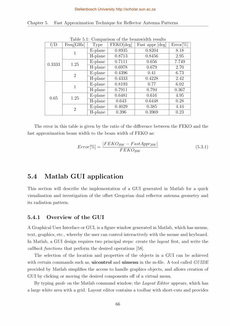
Chapter 5. Fast Approximation Technique for Reflector Antenna Patterns
Table 5.1: Comparison of the beamwidth resultsf/D Freq[GHz] Type FEKO[deg] Fast appr.[deg] Error[%]
0.3333
1E-plane 0.8935 0.8204 8.18H-plane 0.8713 0.8456 2.95
1.25E-plane 0.7111 0.656 7.749H-plane 0.6978 0.679 2.70
2E-plane 0.4396 0.41 6.73H-plane 0.4333 0.4228 2.42
0.65
1E-plane 0.8193 0.77 6.02H-plane 0.7911 0.794 0.367
1.25E-plane 0.6481 0.616 4.95H-plane 0.643 0.6448 0.28
2E-plane 0.4029 0.385 4.44H-plane 0.396 0.3969 0.23
The error in this table is given by the ratio of the difference between the FEKO and the
fast approximation beam width to the beam width of FEKO as:
Error[%] =|FEKOBW − FastApprBW |
FEKOBW
(5.3.1)
5.4 Matlab GUI application
This section will describe the implementation of a GUI generated in Matlab for a quick
visualisation and investigation of the offset Gregorian dual reflector antenna geometry and
its radiation pattern.
5.4.1 Overview of the GUI
A Graphical User Interface or GUI, is a figure window generated in Matlab, which has menus,
text, graphics, etc., whereby the user can control interactively with the mouse and keyboard.
In Matlab, a GUI design requires two principal steps: create the layout first, and write the
callback functions that perform the desired operations [58].
The selection of the location and properties of the objects in a GUI can be achieved
with certain commands such as, uicontrol and uimenu in the m-file. A tool called GUIDE
provided by Matlab simplifies the access to handle graphics objects, and allows creation of
GUI by clicking or moving the desired components off of a virtual menu.
By typing guide on the Matlab command window; the Layout Editor appears, which has
a large white area with a grid. Layout editor contains a toolbar with short-cuts and provides
66
Stellenbosch University http://scholar.sun.ac.za
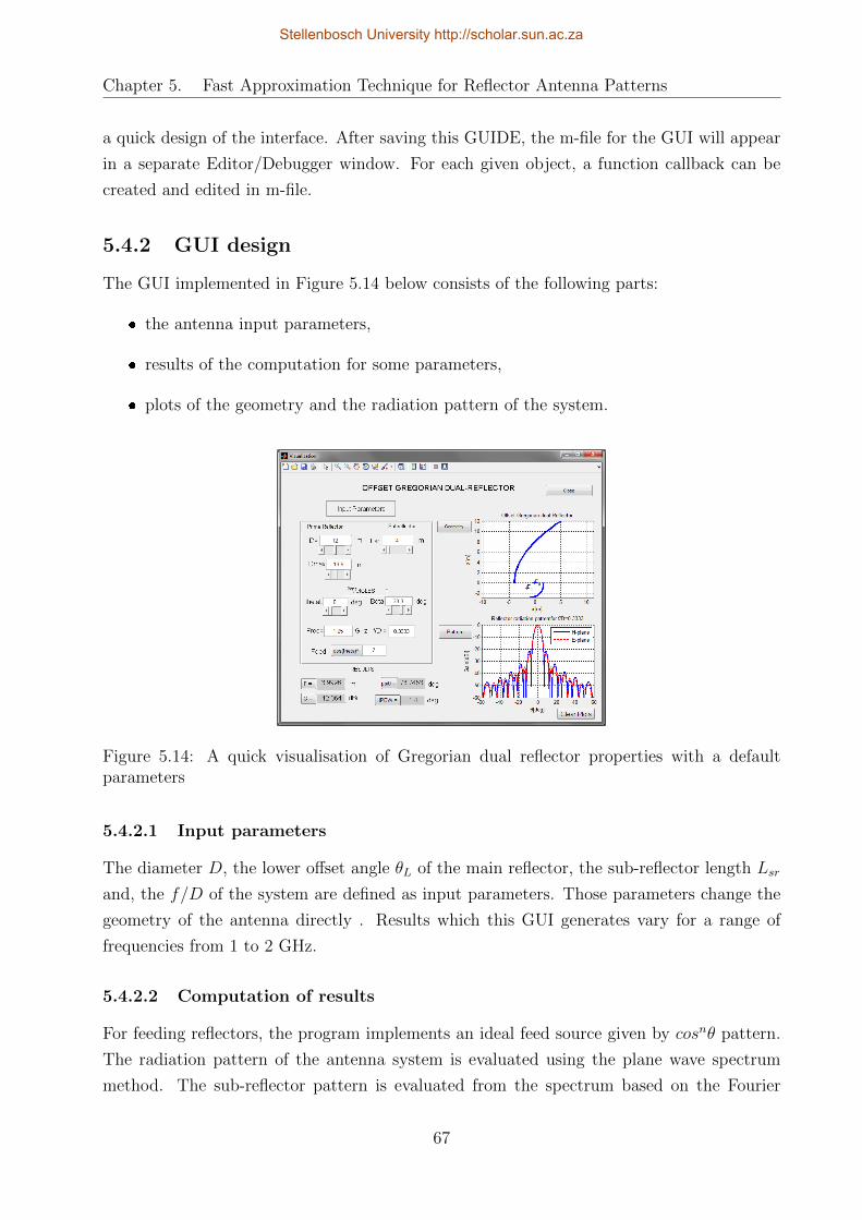
Chapter 5. Fast Approximation Technique for Reflector Antenna Patterns
a quick design of the interface. After saving this GUIDE, the m-file for the GUI will appear
in a separate Editor/Debugger window. For each given object, a function callback can be
created and edited in m-file.
5.4.2 GUI design
The GUI implemented in Figure 5.14 below consists of the following parts:
the antenna input parameters,
results of the computation for some parameters,
plots of the geometry and the radiation pattern of the system.
Figure 5.14: A quick visualisation of Gregorian dual reflector properties with a defaultparameters
5.4.2.1 Input parameters
The diameter D, the lower offset angle θL of the main reflector, the sub-reflector length Lsr
and, the f/D of the system are defined as input parameters. Those parameters change the
geometry of the antenna directly . Results which this GUI generates vary for a range of
frequencies from 1 to 2 GHz.
5.4.2.2 Computation of results
For feeding reflectors, the program implements an ideal feed source given by cosnθ pattern.
The radiation pattern of the antenna system is evaluated using the plane wave spectrum
method. The sub-reflector pattern is evaluated from the spectrum based on the Fourier
67
Stellenbosch University http://scholar.sun.ac.za

Chapter 5. Fast Approximation Technique for Reflector Antenna Patterns
transform, whereby the integral equation can be performed by the FFT algorithm. The
Gauss Legendre technique is used to compute the integral equation of the main reflector
pattern.
5.4.2.3 Plots of the Geometry and Pattern
The plot of the geometry, as well as the patterns and usual antenna parameters, are given
in a well-organized manner on a single page, making it an easy task to compare the features
of the various antenna geometries. The plot in Figure 5.14 shows the radiation pattern of
the entire system in E- and H-plane, the geometry is plotted from the axis system, the gain
of the feed and the 3-dB beam width of the equivalent parabola system.
The creation of this GUI will give the users a quick view of how the changing of the diam-
eter of the reflector affects the gain. Equivalent parabola concepts are applied to investigate
the gain and radiation pattern of the dual reflector antenna.
5.5 Conclusion
The fast approximation for the evaluation of reflector radiation pattern has been discussed
in this chapter. As expected from the formulation the main beam from fast approximation
agree well with the full wave with an error of 6.02% (1 GHz) at low frequency and 0.23%
at 2 GHz for an f/D=0.65. The side lobe levels are not well predicted because of the
complex formulation. The creation of GUI in Matlab is presented to analyse how change the
parameters affect the radiation characteristics.
68
Stellenbosch University http://scholar.sun.ac.za

Chapter 6
Conclusions
Application of two different methods for the investigation of reflector antenna pattern has
been done. The antenna geometry is generated and the radiation pattern is computed using
an hybrid method. The simulation was split into two parts for the two different reflectors
(sub-reflector and main reflector) to get results of greater accuracy and a radiation pattern
point source has been used for the entire simulation to save on computational time and
memory storage.
The radiation properties of this antenna have also been evaluated from a fast approxi-
mation technique based on the plane wave spectrum. The offset geometry was transformed
into its equivalent parabola for this approach. A phase term was added to compensate the
non-planar reflector.
This approach shows that the radiation far-field of the antenna relates to the Fourier
transform of the aperture field and the double integrals of Fourier transform was solved
using the FFT algorithm.
These two approaches are applicable for the reflector antenna analysis. The numerical
computation was done an hybrid method, the feed pattern is used as a point source and
the sub-reflector pattern is computed using MLFMM. Thereafter this sub-reflector pattern
is used as a point source also pointed at the main reflector focal point and PO is applied on
the main reflector.
This method requires an excessive time and memory, while the PWS application is faster
than the hybrid method used in simulation, however it cannot gives any precision for the
side lobes. An interface GUI in Matlab was generated, to give a quick visualisation of
the radiation properties of an offset Gregorian dual reflector antenna using a plane wave
spectrum approach.
69
Stellenbosch University http://scholar.sun.ac.za

Bibliography
[1] S. Gregson, J. McCormick, and C. Parini, Principles of Planar Near-Field Antenna
Measurements. Michael Faraday House Six Hills Way, Stevenage Herts, SG1 2AY,
United Kingdom: Institution of Engineering and Technology, 2007.
[2] P. J. Hall, The Square kilometre Array: An Enginnering Perspective. P.O. Box 17, 3300
AA Dordrecht, The Netherlands: Springer Science, 2005.
[3] S. A. S. K. A. T. P. Office, “South africa’s meerkat a centre of international attention.”
http://www.ska.ac.za/download, March 2011.
[4] J. L. Jonas, “The karoo array telescope,” Cosmology and Galaxy Formation and As-
troparticle Physics on the pathway to the SKA, April 2006.
[5] D. M. Pozar, Microwave and RF design of wireless systems. New York. Toronto. Sin-
gapore: John Wiley & Sons, Inc., 2000.
[6] C. A. Balanis, Antenna Theory: Analysis and Design. Hoboken, New Jersey: John
Wiley & Sons, Inc., 3rd ed., 2005.
[7] “Parabolic reflector basics.” www.radio-electronics.com.
[8] G. A. Thiele and S. W. L., Antenna Theory and Design. John Wiley & Sons, Inc., 1981.
[9] T. C. of IEEE Society, “Ieee standard definitions of terms for antennas,” March 1993.
[10] Y. Huang and K. Boyle, Antennas from Theory to Practice. The Atrium, Southern
Gate, Chichester, West Sussex, PO19 8SQ, United Kingdom: John Wiley & Sons Ltd.,
2008.
[11] P.-S. Kildal, “Factorization of the feed efficiency of paraboloids and cassegrain anten-
nas,” IEEE transactions on antennas and Propagat, vol. 33, pp. 903–908, August 1985.
[12] S. Silver and H. M. James, Microwave Antenna Theory and Design. New York, Tor-
rondo, London: Mc Graw Hill book company, INC., 1949.
70
Stellenbosch University http://scholar.sun.ac.za

Bibliography
[13] http://www.orbitfr.com.
[14] C. F. L. Lew, “Inverted trapezoidal antenna for pulsed application,” Master’s thesis, The
University of Queensland School of Information Technology & Electrical Engineering,
St Lucia, Queensland, 4072, 2003.
[15] A. C. Ludwig, “Definition of cross polarization,” IEEE transactions on antennas and
Propagat, pp. 116–119, January 1973.
[16] T. A. Milligan, Modern Antenna Design. Hoboken, New Jersey: John Wiley & Sons,
PUBLICATION, 2nd edition ed., 2005.
[17] J. D. Kraus and K. R. Carver, Electromagnetics. Mc Graw Hill book company, 2nd ed.,
1981.
[18] B. S. Guru and H. R. Hiziroglu, Electromagnetic Field Theory Fundamentals. The
Edinburgh Building, Cambrige CB2 2RU,UK: Cambrige University Press, 2nd ed., 2004.
[19] http://www.ece.rutgers.edu/ orfanidi/ewa/.
[20] J. Hakli, Shaped Reflector Antenna Design and Antenna Measurements at Sub-mm
Wavelengths. PhD thesis, Helsinki University of Technology, August 2006.
[21] S. AKHMANOV and S. Y. NIKITIN, Physical Optics. Oxford University press. Great
Claredon Street, Oxford ox2 6dp, 1997.
[22] J. Hakli, T. Koskinen, J. Ala-Laurinaho, J. Saily, A. Lonnqvist, J. Mallat, J. Tuovinen,
and A. V. Raisanen, “A dual reflector feed system of a sub-mm hologram catr,” 13th
international symposium on space Terahertz Technology Harvard University, pp. 327–
336, March 2002.
[23] R. G. Kouyoumjian, “Asymptotic high frequency methods,” Proceding IEEE, vol. 53,
pp. 864–876, August 1965.
[24] C. A. Balanis, Advanced Enginnering Electromagnetics. John Wiley & Sons, Inc., 1989.
[25] A. Karttunen, “Design of a 650 ghz dual reflector feed system,” Master’s thesis, Depart-
ment of Electrical and Communications Engineering Helsinki University of Technplogy,
May 2006.
[26] S. Boonsalee, “Effect of random surface errors on the performance of a paraboloid
reflectors,” Master’s thesis, Massachusetts Institute of Technology, February 2000.
[27] M. I. Skolnik, Radar Handbook, vol. 3rd. The McGraw-Hill Companies., 2008.
71
Stellenbosch University http://scholar.sun.ac.za
Bibliography
[28] Y. T. Lo and S. W. Lee, Antenna Handbook Antenna Theory, vol. 2. 115th Avenue New
York, NY 10003: van Nostrand Reinhold, 1993.
[29] W. A. Imbiale and R. E. Hodges, “Linear phase approximation in the triangle facet
near-field physical optics computer program,” Appl. Computational Electromagn. Soc,
vol. 6, no. 2, pp. 74–85, 1991.
[30] C. A. Balanis, Modern Antenna Handbook. 111 River Street, Hoboken, NJ 07030: A
John Wiley & Sons, Inc., Publication, 2008.
[31] M. Born and E. Wolf, Electromagnetic Theory of propagation, interference and diffrac-
tion of light. The Edinburgh Building, Cambrige CB2 2RU, UK: Cambrige University
Press, 7th ed., 1999.
[32] Y. Z. UMUL and U. YALCIN, “Asymptotic evaluation of the edge diffraction in cylindric
paraboloid reflector antennas,” Mathematical and Computational Applications, vol. 8,
no. 2, pp. 143–150, 2003.
[33] J. B. Keller, “Geometrical theory of diffraction,” Journal of the Optical Society of Amer-
ica, pp. 116–130, February 1962.
[34] D. A. McNamara, C. I. Pistorius, and J. G. Malherbe, Introduction to the Uniform
Geometrical Theory of Diffraction. 685 Canton Street Norwood, MA 02062: Artech
House, August 1989.
[35] T.-H. Lee, “Geometrical optical optics and geometrical theory of diffraction analysis of
subreflectors in cassegrain and gregorian reflector antennaa,” Master’s thesis, the Ohio
State Univerity, 1984.
[36] P. Y. Ufimtsev, Fundamentals of the Physical Theory of Diffraction. Hoboken, New
Jersey: JohnWiley & Sons, Inc., 2007.
[37] G. Ahmad and S. A. Mohsin, “High frequency techniques for reflector antenna analysis,”
Electrical Engineering ICEE ’09. Third International Conference, pp. 978–984, July
2009.
[38] A. Michaeli, “Elimination of infinities in equivalent edge currents, part i: Fringe current
components,” IEEE transactions on antennas and Propagat., vol. AP-34, no. 7, pp. 912–
918, 1986.
[39] C. E. RYAN, “Evaluation of edge-diffracted fields including equivalent currents for the
caustic regions,” IEEE transactions on antennas and Propagat., vol. AP-17, no. 3,
pp. 292–299, 1969.
72
Stellenbosch University http://scholar.sun.ac.za

Bibliography
[40] J. P. McKay and Y. Rahmat-Samii, “Compact range reflector analysis using the plane
wave spectrum approach with an adjustable sampling rate,” IEEE transactions on an-
tennas and Propagat, vol. 39, pp. 746–753, June 1991.
[41] R. Clarke and J. Brown, Diffraction Theory and Antennas. Marker Cross House, Cooper
Street, Chichester, West Sussex, PO19 1EB, England: Ellis Horwood Limited, 1980.
[42] P. C. Clemmov, The Plane Wave Spectrum Representation of Electromagnetic Fields.
445 Hoes Lane, PO Box 1331 Plscatawaty NJ 08855-1331: IEEE press, 1966.
[43] T. B. Hansen and A. D. Yaghjian, Plane- wave theory of time-domain fields Near-Field
Scanning Applications. 445 Hoes Lane, PO. Box 1331 Piscataway, NJ 08855-1331: IEEE
Press Series on Electromagnetic Wave Theory, 1999.
[44] E. V. Jull, Aperture Antennas and Diffraction theory. Stevenage, UK and New York:
The Institute of Electrical Enginners, London and New York, 1970.
[45] T. Milligan, “Designing classical offset cassegrain or gregorian dual reflector antennas
from combinations of prescribed geometric parameter,” IEEE transactions on antennas
and Propagat Magazine, vol. 44, pp. 114–123, June 2002.
[46] K. W. Brown and A. P. Jr., “A design procedure for classical offset dual reflector
antennas with circular apertures,” IEEE transactions on antennas and Propagat, vol. 42,
pp. 1145–1153, August 1994.
[47] M. R. SPIEGEL, Mathematical Handbook of Formulas and Tables. Reading, MA:
McGraw-Hill, 1968.
[48] W. V. T. Rusch, L. P. Jr., Y. Rahmat-Samii, and R. A. Shore, “Derivation and applica-
tion of the equivalent paraboloid for classical offset cassegrain and gregorian antennas,”
IEEE transactions on antennas and Propagat, vol. 38, pp. 1141–1149, August 1990.
[49] S. Xu and Y. Rahmat-Samii, “A novel beam squint compensation technique for circu-
larly polarized conic-section reflector antennas,” IEEE transactions on antennas and
Propagat, vol. 58, pp. 307–317, February 2010.
[50] D. I. L. de Villiers, “Analytical prediction of feed efficiency in offset gregorian reflector
antennas with non planar log-periodic type feeds,” PIERS online, vol. 7, pp. 231–235,
2011.
[51] V. Jamnejad-Dailami and Y. Rahmat-Samii, “Some important geometrical features of
conic-section- generated offset reflector antennas,” IEEE transactions on antennas and
Propagat, vol. 28, pp. 952–957, November 1980.
73
Stellenbosch University http://scholar.sun.ac.za
Bibliography
[52] D. B. Davidson, Computational Electromagnetics for RF and Microwave Engineering.
The Edinburgh Building, Cambridge CB2 8RU, UK: Cambrige University press, 2005.
[53] Feko, “Em software & systems-s.a. (pty) ltd.” http://www.feko.info.
[54] A. Tzoulis and T. F. Eibert, “Combining the multilevel fast multipole method with the
uniform geometrical theory of diffraction,” Advances in Radio Science, no. 3, pp. 183–
188, 2005.
[55] R. Chen, P. Rui, and Y. N. Gan, “Schwarz-krylov subspace method for mlfmm analysis
of electromagnetic wave scattering problems,” Progress in electromagnetics research,
vol. pier 82, pp. 51–63, 2008.
[56] A. Z. Nezhad, Z. H. Firouzeh, and H. Mirmohammad-Sadeghi, “A fast method to com-
pute radiation fields of shaped reflector antennas by fft,” Advanced Microwave and Mil-
limeter Wave Technologies: Semiconductor Devices and Circuits and Systems, pp. 190–
204.
[57] P.-S. KILDAL, “The effects of subreflector diffraction on the aperture efficiency of a con-
ventional cassegrain antenna- an analytical approach,” IEEE transactions on antennas
and Propagat, vol. AP-31, no. 6, pp. 903–909, 1983.
[58] R. Brian, H. Ronald, L. Lipsman, J. M. Rosenberg, K. R. Coombes, J. E. Osborn, and
G. J. Stuck, A Guide to MATLAB for Beginners and Experienced Users. Cambrige
University Press, 2001.
74
Stellenbosch University http://scholar.sun.ac.za

Appendices
75
Stellenbosch University http://scholar.sun.ac.za

Appendix A
Analytical evaluation of directivity
using spectrum [1].
A.1 Directivity using PWS
The directivity of a reflector antenna can be compute from the feed pattern. It is defined as
the ratio of the maximum radiation intensity of the antenna over the radiated power divided
by unit of the solid angle.
D = 4πUmaxPrad
(A.1.1)
This radiation intensity is proportional to the far electric field as:
U(θ, φ) =r2
2η|E(r, θ, φ)|2 (A.1.2)
in which the far field, the electric field can be expressed as:
E(r, θ, φ) =e−jkr
rE(θ, φ) (A.1.3)
where r is the radius and (θ, φ) is the angle in the far field. By replacing the electric field on
each value given by (A.1.3). Then, (A.1.2) is reduced into:
U =1
2η|E(θ, φ)| (A.1.4)
A–1
Stellenbosch University http://scholar.sun.ac.za

Appendix A. Analytical evaluation of directivity using spectrum [1].
The electric field also can be evaluated from the angular spectrum and it is expressed in
rectangular coordinates as:
E(x, y, z) =1
4π2
∫ ∞−∞
∫ ∞−∞
F (kx, ky)e−j(kxx+kyy+kzz)dkxdky (A.1.5)
where F (kx, ky) describes the plane wave spectrum of the field; and (A.1.5) defines the
relationship between the near-field zone and the far field for a planar systems.
A.2 The total radiated power
The time averaged power flux that is transmitted per unit area across an aperture plane,
radiated by an arbitrary current density can be given by:
Pr =1
2Re
∫(ET ×H∗T ).ezdxdy
(A.2.1)
Taking the cross product of the tangential electric field and the complex conjugate of the
tangential magnetic field yields.
(ET ×H∗T ) .ez =
∣∣∣∣∣∣∣ex Ex Hx
ey Ey Hy
ez 0 0
∣∣∣∣∣∣∣ .ez =(ExH
∗y − EyH∗x
)(A.2.2)
Then (A.2.1) becomes:
Pr =1
2Re
∫ExH
∗ydxdy
− 1
2Re
∫(EyH
∗xdxdy
(A.2.3)
and from the Parseval’s theorem [1], the total radiated power is given as:
Pr =1
8π2Re
∫ ∞−∞
∫ ∞−∞
ExH∗ydkxdky
− 1
8π2Re
∫ ∞−∞
∫ ∞−∞
EyH∗xdkxdky
(A.2.4)
A–2
Stellenbosch University http://scholar.sun.ac.za


