1
Finite Element Analysis of the ACL-deficient Knee
David Jorge Carvalho Fernandes
IST, Universidade de Lisboa, Portugal
December 2014
Abstract
Anterior cruciate ligament (ACL) rupture is a serious injury whose frequency has been increasing in the last few
years. To understand the causes and consequences of this injury it is fundamental to know the role of the ACL in the
knee.
This work aims to analyze the knee behavior after an ACL rupture, through the finite element method. For this
purpose, it is used a fully tridimensional model of the tibiofemoral joint, with and without ACL, where loads that evidence
the ligament function are applied.
The knee ligaments were modeled with two hyperelastic constitutive models: The isotropic Marlow and the
anisotropic Holzapfel-Gasser-Ogden (HGO) models. Both material models were fitted using the same uniaxial stress-
strain curves. The parameters of the HGO were estimated with the help of an optimization routine, connecting MATLAB
to Abaqus. The comparison between the results obtained through both the constitutive models allows to conclude that
HGO model can better reproduce the mechanical behavior of the ligaments.
Despite some verified differences in quantitative terms, the finite element model is able to produce kinematic and
force results that confirm the ACL as the main restrainer to anterior tibial (or posterior femoral) translation. Furthermore,
in ACL absence, there is a clear increase in knee laxity in more than one degree of freedom, particularly in internal-
external tibial rotation.
Keywords: Anterior Cruciate Ligament, Knee Joint, Finite Element Method, Biomechanics.
1. Introduction
The knee joint is the largest and most complex joint
in the human body consisting of both femoropatellar and
tibiofemoral joints [1]. The structure of the knee permits
the bearing of very high loads, as well as the mobility
required for locomotor activities [2].
The knee ligaments act as joint stabilizers and
movement restrainers [3]. The anterior cruciate ligament
(ACL) plays a critical role in the physiological kinematics
of the knee joint, being the primary restraint against
anterior tibial translation and also limiting knee
hyperextension [1,4,5]. ACL rupture is a serious and the
most common ligament injury, with an increasing number
of 100 000 to 200 000 incidences per year in the United
States [6]
A sound knowledge of both biomechanics and
kinematics of the knee and the ACL role in it are
indispensable to understand the causes of ACL injuries,
its consequences, how to prevent them and even to
improve surgical procedures. While experimental studies
have limitations such as their high cost and low
reproducibility, computational models are a good
alternative to study several biomechanical quantities with
reduced costs and high time and machinery efficiency. In
particular, finite element (FE) method analysis can
provide accurate and medical relevant results [3,7–9].
The FE simulation technique permits a precise
calculation of both special and temporal variations of
stresses, strains and contact areas/forces in different
situations that can be easily reproduced [8–10].
Therefore, FE analysis are a powerful tool in providing
biomechanical information that can be extremely useful
in a clinical context.
2
1.1. Literature Review
The existing computational FE models of the knee,
vary in diverse parameters, such as the degree of
complexity, the study variables, material models
definitions and loading cases. The choice of the
parameters to study defines the nature of the analysis,
which can be static or quasi-static [3,11,12,7,13–25] or
dynamic, [7,26–30].
Due to the intricate anatomy and structure diversity
of the knee joint, many of the FE studies simplify the
analysis by focusing only on the tibiofemoral joint
[11,12,9,16,18,21,23,25,31,32] and by not including
parts such as the menisci and the articular cartilage
[11,12,9,18,25] or other ligaments [11,12,9,16,25].
Some studies opted for representing the knee
ligaments with one-dimensional (1D) truss/beam
[13,14,26] or spring [16,17,23,24,30] elements with
simplified material properties. Despite the increased
ease in obtaining kinematic and force data, this approach
does not allow to determine the stress distribution in the
ligaments [11,7,33].
When using three-dimensional (3D) representations
of the ligaments, the challenge is to develop a material
model that can completely characterize the nonlinear
behavior of ligaments. To this matter, isotropic
[11,12,19,20,33], transversely isotropic [3,9,15,25,32,34]
and anisotropic hyperelastic material models [7,31] have
been used.
So, it is clear that despite being a widely studied
topic on the FE modeling context, the development of a
trustworthy model of such a complex structure as the
knee joint is a very challenging process. The difficulties
increase even more when a good description of the
ligaments behavior is required.
1.2. Objectives
The overall goal of this work is to develop a 3D FE
model that enables a biomechanical analysis of the knee
behavior after an ACL rupture. In detail, this work aims to
provide clinical relevant information regarding the force,
stress and displacement changes that occur in an ACL
deficient knee.
Another objective is to verify the biomechanical
changes induced by an isotropic and anisotropic
hyperelastic constitutive models in the modeling of the
knee ligaments.
It is expected that the model is able to reproduce
qualitatively and, if possible, quantitatively the behavior
found in the literature in order to form a reliable
foundation for futures FE studies regarding the knee
joint.
2. Methods
The knee joint geometry used in this thesis was
obtained from the Open Knee project. [35,36]. This
includes 3D solid representations of eleven parts of the
tibiofemoral joint: distal femur, proximal tibia, articular
cartilages (femoral, medial tibial, and lateral tibial),
anterior cruciate ligament (ACL), posterior cruciate
ligament (PCL), medial collateral ligament (MCL) and
lateral collateral ligament (LCL) and the medial and
lateral menisci.
The bones were defined as rigid bodies due to their
much greater stiffness in comparison to soft tissues and
meshed with quadrilateral and triangular shell elements.
The remaining tissues were meshed with hexaedral
(C3D8) elements.
Articular cartilage was modeled as linear elastic
isotropic material. Despite being a hydrated tissue, the
time of interest of the loading cases discussed in this
thesis is too small compared to the viscoelastic time
constant of cartilage (1 s versus 1500 s), making this a
reasonable approximation. The same approach has
been adopted in many other studies [3,7,14,16,17,19–
22,26,30]. From the different values available in the
literature, the Young’s modulus (E) and Poisson’s ratio
(𝜐) of the articular cartilage were chosen to be 5 MPa
[3,17,21,22] and 0.46 [3,21], respectively. The same
explanation goes for the menisci, for which was assumed
E=59 MPa and 𝜐=0.49 [3,21]. The viscoelastic behavior
of the ligaments was also neglected. However,
considering their highly non-linear stress-strain behavior
and the information found in the literature with respect to
their material modeling, it would be too simplistic to
describe the ligaments with linear elastic properties.
Therefore, two hyperelastic constitutive models available
in the material set library of Abaqus were tested: the
Marlow and the Holzapfel-Gasser-Ogden (HGO)
constitutive models.
The Marlow model, developed by R.S. Marlow [37],
is a general first-invariant hyperelastic constitutive
model, whose strain energy density function Ψ (SEDF)
depends exclusively on the first-invariant, 𝐼 and is
presented in Eq. 1.
Ψ(𝐼1̅) = ∫ 𝑇(𝜀) 𝑑𝜀𝜆𝑇(𝐼1̅)−1
0 (1)
Where 𝑇(𝜀) is the nominal uniaxial traction, 𝜆𝑇(𝐼1̅) is
the uniaxial stretch and 𝜀 is the uniaxial strain. The
incompressibility constraint is introduced by 𝐼1̅, which is
the isochoric part of the first strain invariant, 𝐼1.
To adjust this model to a given stress-strain curve in
Abaqus (Simulia, Providence, USA), we need only to
provide the experimental stress-strain data points, which
will substitute the term 𝑇 and, therefore, there is no need
3
of a curve-fitting procedure. By doing this, the curve
created by the modelwill pass in each of the points given,
reproducing exactly the stress-strain behavior used in its
definition.
The HGO constitutive model was developed by
Gasser et al. [38] to describe the histology and
mechanical properties of arterial tissue. By adding a
scalar parameter to account for the dispersion of
collagen fibers to a previous structural framework
[39,40], they defined a model especially suited to
describe the anisotropic hyperelastic behavior of
collagen fiber reinforced materials, such as the
ligaments. Considering that the material to model
consists of two families of fibers, each of the families can
be characterized by a mean referential (preferred)
direction about which the fibers are distributed with
rotational symmetry. The two distinct directions in the
reference configuration are defined in terms of two unit
vectors 𝒂0𝑖 , 𝑖 = 4,6. This allows the definition of two
additional invariants:
𝐼4 = 𝒂04 ⋅ (𝑪𝒂04), 𝐼6 = 𝒂06 ⋅ (𝑪𝒂06) (2)
With these concepts in mind, the SEDF of the HGO
model for the incompressible case is presented in Eq.
(3):
Ψ = 𝐶10(𝐼1̅ − 3) + 𝑘1
𝑘2
∑ {𝑒𝑘2(�̅�𝑖) − 1}𝑁𝑖 (3)
Where,
�̅�𝑖 ≝ 𝜅(𝐼1̅ − 3) + (1 − 3𝜅)(𝐼(̅𝑖) − 1) (4)
The first term in Eq. (3) serves to model the non-
collagenous ground matrix by means of a neo-Hookean
incompressible isotropic model while the second term
accounts for the families of fibers with different directions
embedded in the ground matrix.
𝑁 (≤ 3) is the number of fiber families. For 𝑁 = 2, we
can set 𝑖 = 4,6 and the term 𝐼(̅𝑖) can be substituted in Eq.
(4) by the isochoric parts of the invariants defined in Eq.
(2).
𝐶10, 𝐷, 𝑘1, 𝑘2 are the parameters of the model that
change the stress-strain response to model different
materials.
𝜅 is the parameter that controls the dispersion
around the mean direction of each family of fibers. When
𝜅 = 0, the fibers are perfectly aligned in the preferential
direction. As the value increases, the fiber dispersion
also increases until 𝜅 reaches 13⁄ , which represents
randomly distributed fibers (isotropic situation).
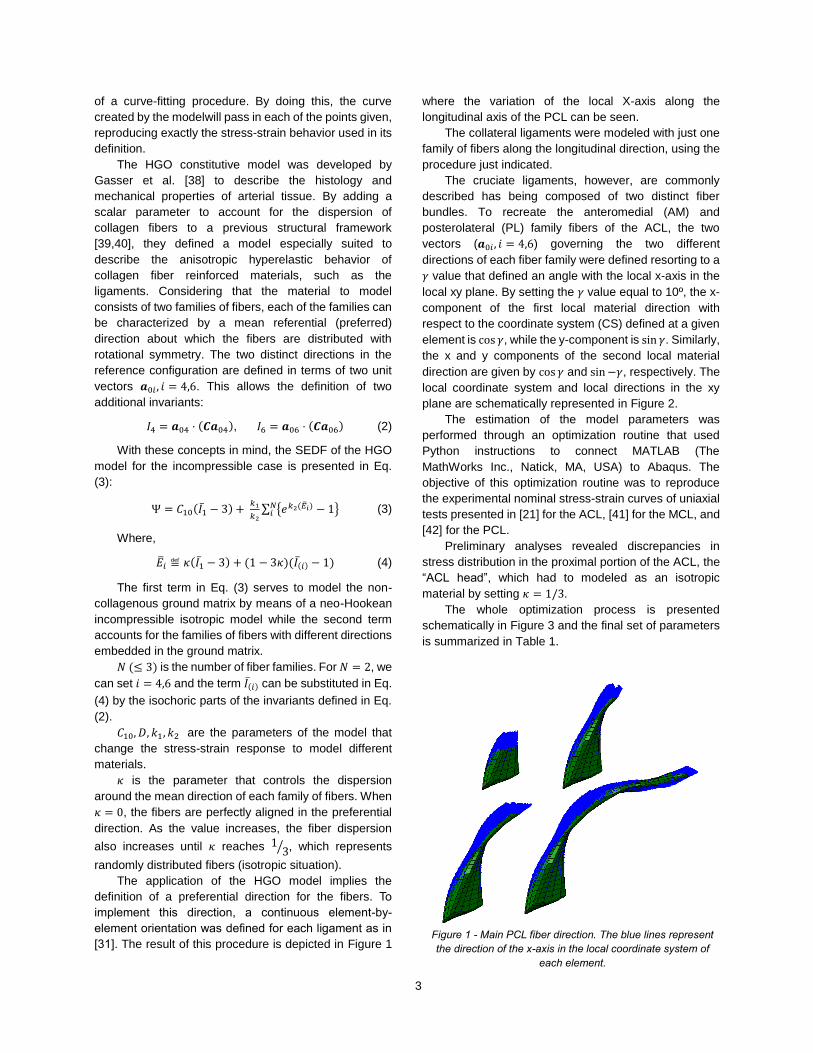
The application of the HGO model implies the
definition of a preferential direction for the fibers. To
implement this direction, a continuous element-by-
element orientation was defined for each ligament as in
[31]. The result of this procedure is depicted in Figure 1
where the variation of the local X-axis along the
longitudinal axis of the PCL can be seen.
The collateral ligaments were modeled with just one
family of fibers along the longitudinal direction, using the
procedure just indicated.
The cruciate ligaments, however, are commonly
described has being composed of two distinct fiber
bundles. To recreate the anteromedial (AM) and
posterolateral (PL) family fibers of the ACL, the two
vectors (𝒂0𝑖 , 𝑖 = 4,6) governing the two different
directions of each fiber family were defined resorting to a
𝛾 value that defined an angle with the local x-axis in the
local xy plane. By setting the 𝛾 value equal to 10º, the x-
component of the first local material direction with
respect to the coordinate system (CS) defined at a given
element is cos 𝛾, while the y-component is sin 𝛾. Similarly,
the x and y components of the second local material
direction are given by cos 𝛾 and sin −𝛾, respectively. The
local coordinate system and local directions in the xy
plane are schematically represented in Figure 2.
The estimation of the model parameters was
performed through an optimization routine that used
Python instructions to connect MATLAB (The
MathWorks Inc., Natick, MA, USA) to Abaqus. The
objective of this optimization routine was to reproduce
the experimental nominal stress-strain curves of uniaxial
tests presented in [21] for the ACL, [41] for the MCL, and
[42] for the PCL.
Preliminary analyses revealed discrepancies in
stress distribution in the proximal portion of the ACL, the
“ACL head”, which had to modeled as an isotropic
material by setting 𝜅 = 1/3.
The whole optimization process is presented
schematically in Figure 3 and the final set of parameters
is summarized in Table 1.
Figure 1 - Main PCL fiber direction. The blue lines represent
the direction of the x-axis in the local coordinate system of
each element.

4
Eleven locations of potential contact were identified
(femoral cartilage to tibial cartilage, cartilages to menisci,
ligaments to bones and ACL to PCL.). Each contact pair
interaction was defined as Surface-to-Surface Contact
with frictionless finite sliding between each contact pair
as in [3,7,16,17,21,22].
2.1. Loads and Boundary Conditions
The model was aligned with a coordinate system
(CS) consistent with a CS commonly used to describe
the tibiofemoral joint movements. In this CS, origin is
defined as the mid-point of the femoral condyles, the x-
axis is flexion axis, the y-axis is the anterior-posterior axis
and the z-axis represents the mechanical axial axis.
A posterior load of 134 N was applied to the healthy
knee, in the Reference Point (RP) that controlled the rigid
body motion of the femur at 0, 15 and 30º of flexion.
Due to the large displacements of the femur in ACL
absence, the value of the force applied in the ACL-
deficient knee was reduced to half.
These loading conditions were designed to simulate
clinical examinations used to diagnose ACL deficiency,
such as the Lachman test [43] and to compare the knee
kinematics at different angles of flexion with the
experimental data.
During the application of the force, the flexion-
extension degree of freedom (DOF) of the femur was
fixed and the tibia was fixed in all DOFs. Therefore, the
posterior displacement of the femur relative to the tibia is
equivalent to the anterior tibial translation relative to the
femur that happens during clinical evaluations of the ACL
function.
Each of the distal ends of the four ligaments were
constrained to a different RP by a Kinematic Coupling
constraint. These reference points were fixed in all
degrees of freedom. In this way, the reaction force
measured on each RP would represent the in situ force
taken up by each ligament in response to tibial motion.
Table 1 - Final set of parameters of the HGO model for each
ligament.
𝑪𝟏𝟎/MPa 𝒌𝟏/MPa 𝒌𝟐 𝜿 Fiber
Fam.
ACL
(body) 0.117 30.779 8.411 0.066 2
ACL
(head) 20.000 2912.833 0.100 1/3 2
PCL 0.011 7.826 446.198 0.057 2
MCL &
LCL 0.213 61.344 18.706 0.085 1
3. Results and Discussion
For each of the flexion angles mentioned, the results
presented are: the kinematic results in terms of tibial
relative displacement; the magnitude of the reaction
force at the tibial insertion of each ligament and the
Figure 3 - Diagram of the optimization process of the HGO
model parameters. Adapted from [48].
Parameter Initialization, c0
Simulated FE uniaxial tension test in Abaqus
Best Fit?
End
Update parameter set using MATLAB
function lsqcurvefit
No
Yes
(𝐶10, 𝑘1, 𝑘2,, 𝜅 , 𝑖𝑡𝑒𝑟)
Figure 2 - Schematic representation of the local coordinate
system used in each element of the ACL to define the direction
of the two fiber families. Considering the planes 567, 145 and
236 as the anterior, medial and lateral planes, the AM and PL
bundles of the ACL can be defined in the local coordinate
system represented. The smaller lines around the AM and PL
directions represent the dispersion of the collagen fibers
direction, controlled by the κ parameter.

5
maximum principal stress at each ligament, calculated as
an average of the nodal stresses of the corresponding
ligament. For the case where the knee is at 30º of flexion,
both anterior (or lateral, in the ACL-deficient knee) and
medial views of the tibiofemoral joint are also presented,
showing the maximum principal stress of the soft tissues.
The comparison between the two materials models
was made only for the knee in full extension. For higher
flexion angles, only the HGO model was considered.
3.1. ACL-Intact Knee
3.1.1. Full Extension (0º of Flexion)
The kinematic, force and stress results for the ACL-
intact knee at full extension using both material models
are presented in Figure 5 and Table 2, respectively.
Table 2 - Ligaments reaction force and average maximum
principal stress in the ACL-intact knee at full extension under a
134 N posterior femoral force.
The comparison between the two material models
shows that with the Marlow model, there is less
movement in all DOFs. This was an expected result,
since this model defines the ligaments as isotropic
materials, and consequently, their resistance to
longitudinal and transverse loads is the same, thus
providing more restrain in each direction.
This behavior is also expressed by the forces taken
up by each ligament. In the Marlow model, the ACL is
less loaded than in the HGO model and the contrary
happens to the other ligaments due to their ability to
sustain loads in directions other than in the longitudinal
one. The simulations with the HGO model show a better
agreement with the experimental data than the
simulations with the Marlow model, with all the
displacements falling in the region delimited by the
standard deviation. The exception to this is the distal
translation (U3), which is slightly above the superior limit
of the standard deviation.
For a more reliable model validation, it is mentioned
the experimental data obtained by other authors when
applying the same 134 N force. For anterior tibial
translation, the values obtained by Yagi et. [44], Song et
al. [12] and Kanamori et al. [45] were, respectively, 4.1 ±
0.6, 4.6 and 5.3 ± 1 mm. For internal rotation of the tibia,
Song et al. reports 1.6º while Kanamori et al. refers 2.1 ±
3.1º.The anterior tibial translation obtained in the FE
simulation was less than the experimental average
values, which might suggest that the ACL was modeled
a bit too stiffer than it should be. This topic is further
discussed in the following sections.
ACL LCL MCL PCL
Reaction
Force (Mag.)
/N
HGO 133.20
0 0.757 7.906
0.007
Marlow 121.71
9 5.844 13.037
3.228
Avg. Max.
Princ. Stress/MPa
HGO 11.350 0.130 0.578 0.00
1
Marlow 10.000 1.368 0.967 0.29
0
Figure 4 - Mesh of the fully assembled knee aligned with the new coordinate system and with the femoral RP highlighted.
Different colors represent different tissues: grey for bones, blue for articular cartilages, yellow for menisci and green for
ligaments. (Left) Anterior view. (Right) Posterior view.
6
Regarding the ACL in situ force, all the three
experimental studies above mentioned report values
between 115 and 140 N, validating the value of 133.2 N
obtained in the simulations.
As for the ligament stresses, there was not much
data available in the literature. In experimental tests
using cadaveric knees it is difficult to accurately measure
the stress. In the case of FE studies, the lack of data is
related to the fact that many of them use one dimensional
(truss/beam or spring) elements to model the ligaments,
which cannot give stress information. Nevertheless, the
values obtained for the ACL seem to be within the range
of values reported in two FE studies simulating similar
loading conditions: Peña et al. [3] obtained an average
maximal principal stress of 6.5 MPa for the ACL and a
maximum value of 15 MPa, while Song et al. [12]
obtained an average value of 6.9 MPa and a maximum
value of 24 MPa.
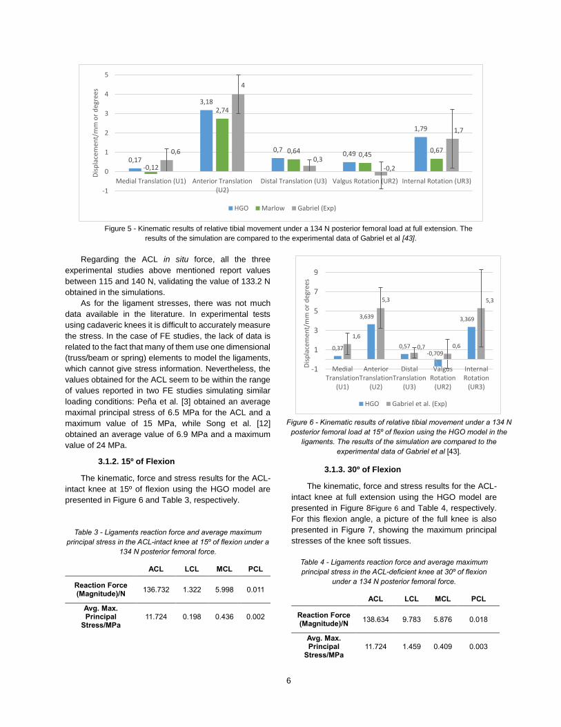
3.1.2. 15º of Flexion
The kinematic, force and stress results for the ACL-
intact knee at 15º of flexion using the HGO model are
presented in Figure 6 and Table 3, respectively.
Table 3 - Ligaments reaction force and average maximum
principal stress in the ACL-intact knee at 15º of flexion under a
134 N posterior femoral force.
ACL LCL MCL PCL
Reaction Force (Magnitude)/N
136.732 1.322 5.998 0.011
Avg. Max. Principal
Stress/MPa 11.724 0.198 0.436 0.002
3.1.3. 30º of Flexion
The kinematic, force and stress results for the ACL-
intact knee at full extension using the HGO model are
presented in Figure 8Figure 6 and Table 4, respectively.
For this flexion angle, a picture of the full knee is also
presented in Figure 7, showing the maximum principal
stresses of the knee soft tissues.
Table 4 - Ligaments reaction force and average maximum
principal stress in the ACL-deficient knee at 30º of flexion
under a 134 N posterior femoral force.
ACL LCL MCL PCL
Reaction Force (Magnitude)/N
138.634 9.783 5.876 0.018
Avg. Max. Principal
Stress/MPa 11.724 1.459 0.409 0.003
0,17
3,18
0,70,49
1,79
-0,12
2,74
0,64 0,450,670,6
4
0,3-0,2
1,7
-1
0
1
2
3
4
5
Medial Translation (U1) Anterior Translation(U2)
Distal Translation (U3) Valgus Rotation (UR2) Internal Rotation (UR3)
Dis
pla
cem
ent/
mm
or
deg
rees
HGO Marlow Gabriel (Exp)
Figure 5 - Kinematic results of relative tibial movement under a 134 N posterior femoral load at full extension. The
results of the simulation are compared to the experimental data of Gabriel et al [43].
Figure 6 - Kinematic results of relative tibial movement under a 134 N
posterior femoral load at 15º of flexion using the HGO model in the
ligaments. The results of the simulation are compared to the
experimental data of Gabriel et al [43].
0,37
3,639
0,57-0,709
3,369
1,6
5,3
0,7 0,6
5,3
-1
1
3
5
7
9
MedialTranslation
(U1)
AnteriorTranslation
(U2)
DistalTranslation
(U3)
ValgusRotation
(UR2)
InternalRotation
(UR3)
Dis
pla
cem
ent/
mm
or
deg
rees
HGO Gabriel et al. (Exp)

7
At 30º, the FE kinematic results (Figure 8) are again
in accordance to the experimental data of Gabriel et al,
except for the valgus rotation. Both anterior tibial
translation and internal rotation continue to increase as
the flexion angle goes from 15 to 30º. This is concomitant
with the higher force magnitude of the ACL, which is
more requested as the flexion angle increases (in the
range of flexion considered). At this angle of flexion, Yagi
et al. [44] and Kanamori et al. [45] obtained an anterior
tibial displacement of 6.4 ± 2.4 mm and 10.1 ± 3.8 mm,
respectively. For the ACL in situ force, the same authors
report values ranging from 106 to 155 N.
By comparing the simulation results with all sets of
experimental data for this flexion angle, we can again
verify that the model underpredicts anterior tibial
translation, supporting the hypothesis of increased ACL
stiffness posed earlier.
Making a global analysis of the results obtained for
the ACL-intact knee, it is reasonable to say that the
model provides kinematic outputs that are qualitatively
(and mostly quantitatively) consistent with the
experimental data except for the valgus-varus rotation.
The remaining DOFs, despite some differences in terms
of absolute values (as it happens with the
underprediction of the anterior tibial movement) are
almost always within the range of values indicated and
tend to follow the behavior reported in the literature.
The results of the ACL in situ forces are also in good
agreement with the literature values. For the other
ligaments, the only data found was again from Kanamori
et al [45] which reports values between 14 and 15 N for
the MCL in situ forces for all the range of flexion here
considered. The obtained values were lower than this.
While on one hand this could also point to some change
to be made to the ligament properties, on the other hand,
it would be interesting to have more experimental data
on this matter to draw more solid conclusions.
The validity of the stress results is more difficult to
evaluate due to the lack of experimental data, but when
in comparison to similar FE simulations, the obtained
average values seem to be in the correct interval of
values, at least when the knee is in full extension.
Figure 8 - Kinematic results of relative tibial movement under a
134 N posterior femoral load at 30o of flexion using the HGO
model in the ligaments. The results of the simulation are
compared to the experimental data of Gabriel et al [43].
0,735
4,017
0,474 -2,066
4,535
2,2
5,9
1 1,6
7,6
-3
-1
1
3
5
7
9
11
13
MedialTranslation
(U1)
AnteriorTranslation
(U2)
DistalTranslation
(U3)
ValgusRotation
(UR2)
InternalRotation
(UR3)
Dis
pla
cem
ent/
mm
or
deg
rees
HGO Gabriel et al. (Exp)
Figure 7 - ACL-intact knee joint at 30º of flexion after the application of a 134 N posteriorly directed force on
the femur using the HGO material model in the ligaments. (Left side) Anterior view. (Right side) Medial view.

8
3.2. ACL-Deficient Knee
3.2.1. Full Extension (0º of Flexion)
The kinematic, force and stress results for the ACL-
deficient knee at full extension, using both material
models are presented in Figure 9 and Table 5,
respectively.
Table 5 - Ligaments reaction force and average maximum
principal stress in the ACL-intact knee at full extension under a
67 N posterior femoral force - comparison between the two
material models.
LCL MCL PCL
Reaction Force
(Mag.)/N
HGO w/ ACL
0.279 4.737 0.014
HGO w/o ACL
65.233 70.294 0.014
Marlow w/ ACL
2.513 7.348 1.342
Marlow w/o ACL
41.957 48.57 7.359
Avg. Max. Princ.
Stress/MPa
HGO w/ ACL
0.051 0.351 0.001
HGO w/o ACL
10.851 5.023 0.004
Marlow w/ ACL
0.716 0.551 0.115
Marlow w/o ACL
8.275 3.485 0.787
3.2.2. 15º of Flexion
The kinematic, force and stress results for the ACL-
deficient knee at full extension, using the HGO model are
presented in Figure 10 and Table 6, respectively.
Table 6 - Ligaments reaction force and average maximum
principal stress in the ACL-deficient knee at 15o of flexion
under a 67 N posterior femoral force.
LCL MCL PCL
Reaction Force
(Magnitude)/N
w/ ACL 2.480 5.759 0.019
w/o ACL 67.556 75.001 0.019
Avg. Max. Principal
Stress/MPa
w/ ACL 0.376 0.419 0.001
w/o ACL 11.000 5.370 0.002
Figure 10 - Kinematic results of relative tibial movement under
a 67 N posterior femoral load at 15º of flexion using the HGO
model in the ligaments - comparison between the ACL-intact
and ACL-deficient knees.
-0,009
2,255
0,401-0,173
0,815-0,556
10,998
2,008
0,171
6,509
-1
1
3
5
7
9
11
MedialTranslation
(U1)
AnteriorTranslation
(U2)
DistalTranslation
(U3)
ValgusRotation
(UR2)
InternalRotation
(UR3)
Dis
pla
cem
ent/
mm
or
deg
rees
With ACL Without ACL
0,048
1,91
0,505 0,422 0,558-0,313
9,477
2,204
1,047
4,331
-0,024
1,794
0,521 0,284 0,357-0,132
5,058
1,61
0,367
1,341
-1
1
3
5
7
9
Medial Translation (U1) Anterior Translation(U2)
Distal Translation (U3) Valgus Rotation (UR2) Internal Rotation (UR3)
Dis
pla
cem
ent/
mm
or
deg
rees
HGO With ACL HGO Without ACL Marlow With ACL Marlow Without ACL
Figure 9 - Kinematic results of relative tibial movement under a 67 N posterior femoral load at full extension in ACL-intact
and ACL-deficient knees – comparison between the two material models.
9
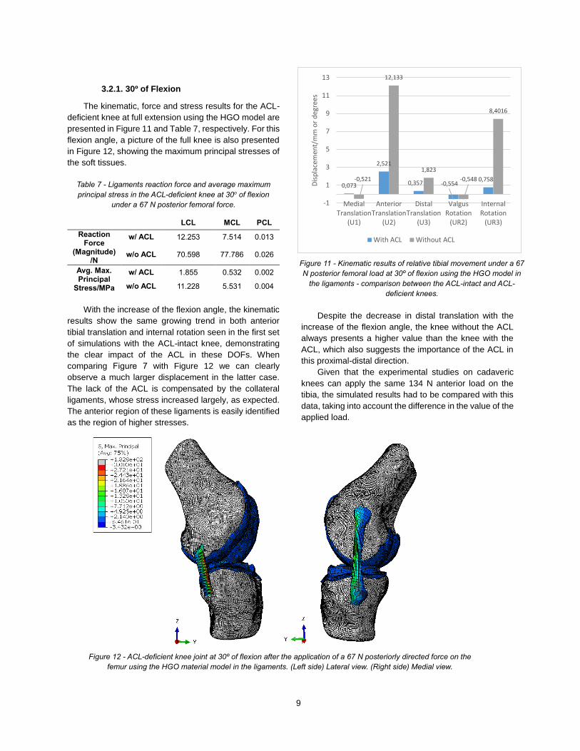
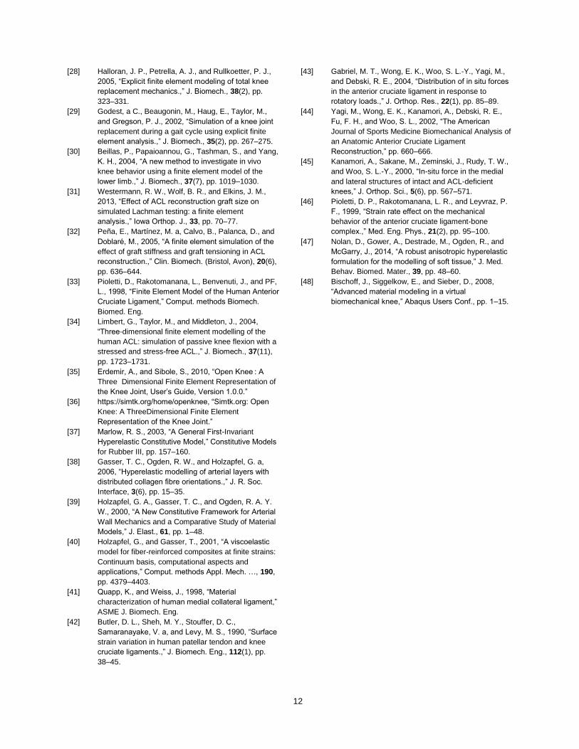
3.2.1. 30º of Flexion
The kinematic, force and stress results for the ACL-
deficient knee at full extension using the HGO model are
presented in Figure 11 and Table 7, respectively. For this
flexion angle, a picture of the full knee is also presented
in Figure 12, showing the maximum principal stresses of
the soft tissues.
Table 7 - Ligaments reaction force and average maximum
principal stress in the ACL-deficient knee at 30o of flexion
under a 67 N posterior femoral force.
LCL MCL PCL
Reaction Force
(Magnitude)/N
w/ ACL 12.253 7.514 0.013
w/o ACL 70.598 77.786 0.026
Avg. Max. Principal
Stress/MPa
w/ ACL 1.855 0.532 0.002
w/o ACL 11.228 5.531 0.004
With the increase of the flexion angle, the kinematic
results show the same growing trend in both anterior
tibial translation and internal rotation seen in the first set
of simulations with the ACL-intact knee, demonstrating
the clear impact of the ACL in these DOFs. When
comparing Figure 7 with Figure 12 we can clearly
observe a much larger displacement in the latter case.
The lack of the ACL is compensated by the collateral
ligaments, whose stress increased largely, as expected.
The anterior region of these ligaments is easily identified
as the region of higher stresses.
Despite the decrease in distal translation with the
increase of the flexion angle, the knee without the ACL
always presents a higher value than the knee with the
ACL, which also suggests the importance of the ACL in
this proximal-distal direction.
Given that the experimental studies on cadaveric
knees can apply the same 134 N anterior load on the
tibia, the simulated results had to be compared with this
data, taking into account the difference in the value of the
applied load.
Figure 11 - Kinematic results of relative tibial movement under a 67
N posterior femoral load at 30º of flexion using the HGO model in
the ligaments - comparison between the ACL-intact and ACL-
deficient knees.
0,073
2,521
0,357 -0,5540,758-0,521
12,133
1,823
-0,548
8,4016
-1
1
3
5
7
9
11
13
MedialTranslation
(U1)
AnteriorTranslation
(U2)
DistalTranslation
(U3)
ValgusRotation
(UR2)
InternalRotation
(UR3)
Dis
pla
cem
ent/
mm
or
deg
rees
With ACL Without ACL
Figure 12 - ACL-deficient knee joint at 30º of flexion after the application of a 67 N posteriorly directed force on the
femur using the HGO material model in the ligaments. (Left side) Lateral view. (Right side) Medial view.

10
For the 134 N anterior load, Kanamori et al. [45]
obtained an anterior tibial displacement of 13.3±1.4,
17.3±1.8 and 18.9±2.3 mm in the ACL-deficient knee at
0, 15 and 30º of flexion, respectively. Similar results were
acquired by Yagi et al. [44] with approximately 12.5 and
19 mm for 0 and 30º of flexion, respectively.
In terms of the in situ forces, Kanamori et al. verified
that after the ACL transection the in situ forces of the
MCL increase significantly from less than 20 N in the
ACL-intact knee case to 36 ± 27 N and 41±16 N at 0 and
30º of flexion, respectively.
Since the value of the applied force in the FE
simulation was only half of the value applied in the
experimental studies mentioned, it seems that the FE
model overpredicts the anterior tibial displacement when
the ACL is removed, as well as the in situ forces in the
MCL This fact, associated with the underprediction of
movement for the same DOF when the ACL is present,
suggests a revision of the ligament properties. For
example, if the stiffness of the collateral ligaments was
increased while the stiffness of the ACL was decreased,
the FE simulation should produce a higher anterior tibial
movement when the ACL is present and a lower value of
the same quantity when the ACL is removed.
The stress-strain properties of the ligaments can
greatly vary with the strain rate at which the uniaxial
tension tests are preformed, as we can attest in [46].
Therefore, one way to try to improve the results would be
to perform the curve fitting procedure to other
experimental stress-strain curves with requirements
described above.
4. Conclusion
In this work, the effect of an ACL rupture in the
overall kinematics and biomechanics of the knee was
studied by comparing the effect of a posterior femoral
force on ACL-intact and ACL-deficient knees.
By comparing the kinematic outcomes of the FE
simulations with two material models, it is concluded that
the HGO model presents more accurate results. This
was expected since the HGO was designed to capture
the anisotropic properties of biologic tissues composed
of collagen fiber bundles, such as the ligaments.
Using this model in the ligaments, the FE model is
able to qualitatively (and mostly quantitatively) reproduce
consistent kinematic results with experimental data in all
degrees of freedom except for the valgus-varus rotation.
These results confirm that the ACL provides the major
constraint to anterior tibial motions and also plays an
important role on restraining internal rotation of the tibia.
These conclusions are also supported by the calculated
force sustained by the four ligaments considered.
When the ACL is absent, the collateral ligaments are
the first structures to be requested to sustain anterior-
posterior forces, with obvious implications in their stress
state. The MCL is the ligament that supports more load
in this situation, in accordance to the role attributed to the
MCL as the secondary restraint to anterior tibial
displacements.
To sum up, it is concluded that the ACL rupture
induces several drastic kinematic changes which have a
great impact on the overall biomechanics of the entire
knee structure.
As usual in this type of simulations, there were some
limitations to this study. For instance, the residual
stresses present on the knee ligaments were not
modeled since the Abaqus does not allow the
prescription of pre-stresses in anisotropic hyperelastic
models. Other shortcoming was that the ACL function
was only tested by applying a posterior femoral load. The
influence of the ACL in other types of movements was
not tested.
Despite these limitations, the FE model developed in
this thesis, based on the overall positive results
produced, should provide a solid basis to further develop
significant work in the biomechanical study of the knee.
In the future, an obvious addition to the model would
be the inclusion of the patellofemoral component. The
meniscal attachments to the tibia could also be more
realistically modeled by defining the meniscal horns as a
set of springs as in [16,22,31].
As for the knee ligaments modeling, it is known that
the ligaments are not completely incompressible tissues.
In a very recent study, Nolan et al. [47] demonstrated that
the HGO model does not correctly characterizes the
compressible anisotropic material behavior. In response
to this fact, they proposed a modified anisotropic model
based on the aforementioned model that is said to predict
more accurately the anisotropic response to hydrostatic
tensile loading. The employment of this new model would
require an additional effort to implement an UMAT
routine in Abaqus, but would also add an extra layer of
realism to the ligaments material properties.
Finally, it would be interesting to verify the ACL role
in more complex loading cases. The simulation of more
dynamic situations like jumping or stair climbing together
with a more detailed analysis of the other soft tissues of
the knee, such as the articular cartilage and the menisci,
would also provide great insights about the ACL-deficient
knee functioning.
5. References
[1] Marieb, E., and Hoehn, K., 2013, Human anatomy &
physiology, Pearson Education, Inc.

11
[2] Hall, S., 2012, Basic Biomechanics, McGraw-Hill,
New York, NY.
[3] Peña, E., Calvo, B., Martínez, M. a, and Doblaré, M.,
2006, “A three-dimensional finite element analysis of
the combined behavior of ligaments and menisci in
the healthy human knee joint.,” J. Biomech., 39(9),
pp. 1686–1701.
[4] Dargel, J., Gotter, M., Mader, K., Pennig, D., Koebke,
J., and Schmidt-Wiethoff, R., 2007, “Biomechanics of
the anterior cruciate ligament and implications for
surgical reconstruction,” Strategies Trauma Limb
Reconstr., 2(1), pp. 1–12.
[5] Kweon, C., Lederman, E. S., and Chhabra, A., 2013,
“Anatomy and Biomechanics of the Cruciate
Ligaments and Their Surgical Implications,” The
Multiple Ligament Injured Knee: A Practical Guide to
Management, G.C. Fanelli, ed., Springer New York,
New York, NY, pp. 17–27.
[6] Siegel, L., Vandenakker-Albanese, C., and Siegel, D.,
2012, “Anterior Cruciate Ligament Injuries: Anatomy,
Physiology, Biomechanics, and Management.,” Clin.
J. Sport Med. Off. J. Can. Acad. Sport Med., 22(4),
pp. 349–355.
[7] Kiapour, A., Kiapour, A. M., Kaul, V., Quatman, C. E.,
Wordeman, S. C., Hewett, T. E., Demetropoulos, C.
K., and Goel, V. K., 2014, “Finite Element Model of
the Knee for Investigation of Injury Mechanisms:
Development and Validation,” J. Biomech. Eng.,
136(1), p. 011002.
[8] Herrera, A., Ibarz, E., Cegoñino, J., Lobo-Escolar, A.,
Puértolas, S., López, E., Mateo, J., and Gracia, L.,
2012, “Applications of finite element simulation in
orthopedic and trauma surgery.,” World J. Orthop.,
3(4), pp. 25–41.
[9] Gardiner, J. C., and Weiss, J. a, 2003, “Subject-
specific finite element analysis of the human medial
collateral ligament during valgus knee loading.,” J.
Orthop. Res., 21(6), pp. 1098–1106.
[10] Kluess, D., Wieding, J., and Souffrant, R., “x Finite
Element Analysis in Orthopaedic Biomechanics,” pp.
151–171.
[11] Xie, F., Yang, L., Guo, L., Wang, Z., and Dai, G.,
2009, “A Study on Construction Three-Dimensional
Nonlinear Finite Element Model and Stress
Distribution Analysis of Anterior Cruciate Ligament,” J.
Biomech. Eng., 131(12), pp. 121007–5.
[12] Song, Y., Debski, R. E., Musahl, V., Thomas, M., and
Woo, S. L.-Y., 2004, “A three-dimensional finite
element model of the human anterior cruciate
ligament: a computational analysis with experimental
validation,” J. Biomech., 37(3), pp. 383–390.
[13] Adouni, M., Shirazi-Adl, A., and Shirazi, R., 2012,
“Computational biodynamics of human knee joint in
gait: from muscle forces to cartilage stresses.,” J.
Biomech., 45(12), pp. 2149–2156.
[14] Bendjaballah, M., Shirazi-Adl, A., and Zukor, D.,
1997, “Finite element analysis of human knee joint in
varus-valgus,” Clin. Biomech., 12(3), pp. 139–148.
[15] Dhaher, Y. Y., Kwon, T.-H., and Barry, M., 2010, “The
effect of connective tissue material uncertainties on
knee joint mechanics under isolated loading
conditions.,” J. Biomech., 43(16), pp. 3118–3125.
[16] Hull, M. L., Donahue, T., Rashid, M., and Jacobs, C.,
2002, “A Finite Element Model of the Human Knee
Joint for the Study of Tibio-Femoral Contact,” J.
Biomech. Eng., 124(3), pp. 273–280.
[17] Li, G., Gil, J., Kanamori, A., and Woo, S. L., 1999, “A
validated three-dimensional computational model of a
human knee joint.,” J. Biomech. Eng., 121(6), pp.
657–662.
[18] Park, H.-S., Ahn, C., Fung, D. T., Ren, Y., and Zhang,
L.-Q., 2010, “A knee-specific finite element analysis of
the human anterior cruciate ligament impingement
against the femoral intercondylar notch.,” J. Biomech.,
43(10), pp. 2039–2042.
[19] Ramaniraka, N. a, Saunier, P., Siegrist, O., and
Pioletti, D. P., 2007, “Biomechanical evaluation of
intra-articular and extra-articular procedures in
anterior cruciate ligament reconstruction: a finite
element analysis.,” Clin. Biomech. (Bristol, Avon),
22(3), pp. 336–343.
[20] Ramaniraka, N. a, Terrier, A., Theumann, N., and
Siegrist, O., 2005, “Effects of the posterior cruciate
ligament reconstruction on the biomechanics of the
knee joint: a finite element analysis.,” Clin. Biomech.
(Bristol, Avon), 20(4), pp. 434–442.
[21] Wan, C., Hao, Z., and Wen, S., 2013, “The Effect of
the Variation in ACL Constitutive Model on Joint
Kinematics and Biomechanics Under Different Loads:
A Finite Element Study,” J. Biomech. Eng., 135(4), p.
041002.
[22] Yao, J., Snibbe, J., Maloney, M., and Lerner, A. L.,
2006, “Stresses and Strains in the Medial Meniscus of
an ACL Deficient Knee under Anterior Loading: A
Finite Element Analysis with Image-Based
Experimental Validation,” J. Biomech. Eng., 128(1), p.
135.
[23] Moglo, K. E., and Shirazi-Adl, a., 2003,
“Biomechanics of passive knee joint in drawer: load
transmission in intact and ACL-deficient joints,” Knee,
10(3), pp. 265–276.
[24] Li, G., Suggs, J., and Gill, T., 2002, “The Effect of
Anterior Cruciate Ligament Injury on Knee Joint
Function under a Simulated Muscle Load: A Three-
Dimensional Computational Simulation,” Ann.
Biomed. Eng., 30(5), pp. 713–720.
[25] Ellis, B. J., Lujan, T. J., Dalton, M. S., and Weiss, J.
A., 2006, “Medial Collateral Ligament Insertion Site
and Contact Forces in the ACL-Deficient Knee,” J.
Orthop. Res., (April), pp. 800–810.
[26] Penrose, J. M. T., Holt, G. M., Beaugonin, M., and
Hose, D. R., 2002, “Development of an accurate
three-dimensional finite element knee model.,”
Comput. Methods Biomech. Biomed. Engin., 5(4), pp.
291–300.
[27] Baldwin, M. a, Clary, C. W., Fitzpatrick, C. K., Deacy,
J. S., Maletsky, L. P., and Rullkoetter, P. J., 2012,
“Dynamic finite element knee simulation for evaluation
of knee replacement mechanics.,” J. Biomech., 45(3),
pp. 474–483.
12
[28] Halloran, J. P., Petrella, A. J., and Rullkoetter, P. J.,
2005, “Explicit finite element modeling of total knee
replacement mechanics.,” J. Biomech., 38(2), pp.
323–331.
[29] Godest, a C., Beaugonin, M., Haug, E., Taylor, M.,
and Gregson, P. J., 2002, “Simulation of a knee joint
replacement during a gait cycle using explicit finite
element analysis.,” J. Biomech., 35(2), pp. 267–275.
[30] Beillas, P., Papaioannou, G., Tashman, S., and Yang,
K. H., 2004, “A new method to investigate in vivo
knee behavior using a finite element model of the
lower limb.,” J. Biomech., 37(7), pp. 1019–1030.
[31] Westermann, R. W., Wolf, B. R., and Elkins, J. M.,
2013, “Effect of ACL reconstruction graft size on
simulated Lachman testing: a finite element
analysis.,” Iowa Orthop. J., 33, pp. 70–77.
[32] Peña, E., Martínez, M. a, Calvo, B., Palanca, D., and
Doblaré, M., 2005, “A finite element simulation of the
effect of graft stiffness and graft tensioning in ACL
reconstruction.,” Clin. Biomech. (Bristol, Avon), 20(6),
pp. 636–644.
[33] Pioletti, D., Rakotomanana, L., Benvenuti, J., and PF,
L., 1998, “Finite Element Model of the Human Anterior
Cruciate Ligament,” Comput. methods Biomech.
Biomed. Eng.
[34] Limbert, G., Taylor, M., and Middleton, J., 2004,
“Three-dimensional finite element modelling of the
human ACL: simulation of passive knee flexion with a
stressed and stress-free ACL.,” J. Biomech., 37(11),
pp. 1723–1731.
[35] Erdemir, A., and Sibole, S., 2010, “Open Knee : A
Three Dimensional Finite Element Representation of
the Knee Joint, User’s Guide, Version 1.0.0.”
[36] https://simtk.org/home/openknee, “Simtk.org: Open
Knee: A ThreeDimensional Finite Element
Representation of the Knee Joint.”
[37] Marlow, R. S., 2003, “A General First-Invariant
Hyperelastic Constitutive Model,” Constitutive Models
for Rubber III, pp. 157–160.
[38] Gasser, T. C., Ogden, R. W., and Holzapfel, G. a,
2006, “Hyperelastic modelling of arterial layers with
distributed collagen fibre orientations.,” J. R. Soc.
Interface, 3(6), pp. 15–35.
[39] Holzapfel, G. A., Gasser, T. C., and Ogden, R. A. Y.
W., 2000, “A New Constitutive Framework for Arterial
Wall Mechanics and a Comparative Study of Material
Models,” J. Elast., 61, pp. 1–48.
[40] Holzapfel, G., and Gasser, T., 2001, “A viscoelastic
model for fiber-reinforced composites at finite strains:
Continuum basis, computational aspects and
applications,” Comput. methods Appl. Mech. …, 190,
pp. 4379–4403.
[41] Quapp, K., and Weiss, J., 1998, “Material
characterization of human medial collateral ligament,”
ASME J. Biomech. Eng.
[42] Butler, D. L., Sheh, M. Y., Stouffer, D. C.,
Samaranayake, V. a, and Levy, M. S., 1990, “Surface
strain variation in human patellar tendon and knee
cruciate ligaments.,” J. Biomech. Eng., 112(1), pp.
38–45.
[43] Gabriel, M. T., Wong, E. K., Woo, S. L.-Y., Yagi, M.,
and Debski, R. E., 2004, “Distribution of in situ forces
in the anterior cruciate ligament in response to
rotatory loads.,” J. Orthop. Res., 22(1), pp. 85–89.
[44] Yagi, M., Wong, E. K., Kanamori, A., Debski, R. E.,
Fu, F. H., and Woo, S. L., 2002, “The American
Journal of Sports Medicine Biomechanical Analysis of
an Anatomic Anterior Cruciate Ligament
Reconstruction,” pp. 660–666.
[45] Kanamori, A., Sakane, M., Zeminski, J., Rudy, T. W.,
and Woo, S. L.-Y., 2000, “In-situ force in the medial
and lateral structures of intact and ACL-deficient
knees,” J. Orthop. Sci., 5(6), pp. 567–571.
[46] Pioletti, D. P., Rakotomanana, L. R., and Leyvraz, P.
F., 1999, “Strain rate effect on the mechanical
behavior of the anterior cruciate ligament-bone
complex.,” Med. Eng. Phys., 21(2), pp. 95–100.
[47] Nolan, D., Gower, A., Destrade, M., Ogden, R., and
McGarry, J., 2014, “A robust anisotropic hyperelastic
formulation for the modelling of soft tissue,” J. Med.
Behav. Biomed. Mater., 39, pp. 48–60.
[48] Bischoff, J., Siggelkow, E., and Sieber, D., 2008,
“Advanced material modeling in a virtual
biomechanical knee,” Abaqus Users Conf., pp. 1–15.


![Article The effect of proprioceptive knee bracing on knee stability …clok.uclan.ac.uk/24655/2/Richards J (2018... · 2019-08-07 · managing knee instability and ACL injury [10]](https://cdn.vdocuments.net/doc/165x107/5eceec997c3c6d2ead67f454/article-the-effect-of-proprioceptive-knee-bracing-on-knee-stability-clokuclanacuk246552richards.jpg)