
Forecasting Daily Supermarket Sales Using Exponentially Weighted Quantile Regression
James W. Taylor
Saïd Business School
University of Oxford
European Journal of Operational Research, 2007, Vol. 178, pp. 154-167.
Address for Correspondence: James W. Taylor Saïd Business School University of Oxford Park End Street Oxford OX1 1HP, UK Tel: +44 (0)1865 288927 Fax: +44 (0)1865 288805 Email: [email protected]
Forecasting Daily Supermarket Sales Using Exponentially Weighted Quantile
Regression
Abstract
Inventory control systems typically require the frequent updating of forecasts for many
different products. In addition to point predictions, interval forecasts are needed to set
appropriate levels of safety stock. The series considered in this paper are characterised by
high volatility and skewness, which are both time-varying. These features motivate the
consideration of forecasting methods that are robust with regard to distributional
assumptions. The widespread use of exponential smoothing for point forecasting in inventory
control motivates the development of the approach for interval forecasting. In this paper, we
construct interval forecasts from quantile predictions generated using exponentially weighted
quantile regression. The approach amounts to exponential smoothing of the cumulative
distribution function, and can be viewed as an extension of generalised exponential
smoothing to quantile forecasting. Empirical results are encouraging, with improvements
over traditional methods being particularly apparent when the approach is used as the basis
for robust point forecasting.
Keywords: Forecasting; Exponential smoothing; Quantile regression; Interval forecasting;
Robust point forecasting

1
1. Introduction
When forecasting for inventory control, predictions are very often required at
frequent intervals for many different products or parts. This motivates the automation of
some or all of the forecasting process. The case that we consider is one of forecasting daily
observations of supermarket sales. The data is taken from an outlet of a large UK
supermarket chain, which typically stocks more than 10,000 different items in each of its
stores. The 256 time series in our sample are characterised by high volatility, strong intra-
week seasonality and, for most of the series, fairly low volume. Few of the series exhibit
trend. The high volatility is evident in Figure 1, which is a plot of one of the series. The
figure also shows that sales is positively skewed for many of the days, which is
understandable, given that the series is obviously bounded below by zero.
---------- Figure 1 ----------
Exponential smoothing is a simple and pragmatic approach to point forecasting
whereby the forecast is constructed from an exponentially weighted average of past
observations. The impressive performance of exponential smoothing methods, when applied
across a variety of different series (see, for example, Makridakis and Hibon, 2000), has led to
their widespread use in applications, such as ours, where a large number of series necessitates
an automated procedure. Indeed, our collaborating company currently uses exponential
smoothing, albeit a non-standard method.
Interval forecasting is important for inventory control because it enables the setting of
appropriate levels of safety stock. A common approach to interval forecasting is to use a
point forecast with an estimate of the forecast error distribution. For the widely used
exponential smoothing methods, Hyndman et al. (2005) provide theoretical forecast error
variance formulae, which they derive by referring to the equivalent state-space models. A
Gaussian assumption is then used to deliver prediction intervals. However, the Gaussian
assumption is often not realistic. Indeed, the shape of the distribution may not even be

2
constant over time. This appears to be the case in Figure 1, where the skewness is more
evident when the series is closer to zero. The variance is very often also not constant over
time, and may possess a seasonal pattern independent of seasonality in the mean. A problem
with the use of theoretical error variance formulae is that they are not readily available for
non-standard exponential smoothing approaches, such as the one used by our collaborating
company. In reviewing the prediction interval literature, Chatfield (1993) observes that when
theoretical formulae are not available, or there are doubts about model assumptions, empirically
based methods should be considered. Gardner (1988) and Taylor and Bunn (1999) provide such
methods, but, unfortunately, these methods are not able to accommodate a distribution with
changing shape or variance.
In essence, the supermarket sales case presents the challenge of trying to produce, in
an automated way, interval forecasts for distributions that have changing location, variance
and shape. Rather than base estimation on a point forecast, in this paper, we address the
problem by directly forecasting the sales quantiles. The θ quantile of a variable, yt, is defined
as the value, Qt(θ), for which P(yt≤Qt(θ))=θ. Interval forecasts can be constructed from
forecasts of symmetric quantiles, Qt(θ) and Qt(1-θ). Directly forecasting quantiles avoids the
need for assumptions regarding the spread and shape of the distribution. In view of the
success of exponential smoothing methods for point forecasting within automated
applications, there is strong appeal to developing the approach for interval forecasting. We
do this through the use of exponentially weighted quantile regression (EWQR), which is
equivalent to exponential smoothing of the cumulative distribution function (cdf). Our
application of EWQR provides new insight into the method because the only previous use of
the approach was for the somewhat different application of value at risk estimation in finance
(see Taylor, 2006).
The non-Gaussian nature of the sales series also motivates consideration of point
forecasting methods that are robust to the distributional shape. We propose that robust point

3
forecasts be constructed from the weighted average of EWQR forecasts of several quantiles,
such as the 0.25, 0.50 and 0.75 quantiles.
Section 2 reviews the existing approaches to univariate quantile modelling. In Section 3,
we discuss EWQR and its use for univariate quantile forecasting and robust point forecasting. In
Section 4, we use the method for point forecasting of the supermarket series, and in Section 5
we consider interval forecasting. Section 6 provides a summary and concluding comments.
2. Quantile modelling methods
The value at risk (VaR) literature is concerned with estimating the tail quantiles of
distributions of financial returns. By contrast with our sales series, a series of financial returns
tends to have a mean that is almost constant. Nevertheless, some of the VaR methods can at
least provide insight for our case. Boudoukh et al. (1998) describe their approach as being the
analogy of exponentially weighted moving averages for quantiles. Their method involves
allocating to the most recent year of daily returns, exponentially decreasing weights, which
sum to one. The returns are then placed in ascending order and, starting at the lowest return,
the weights are summed until θ is reached. The θth quantile estimate is set as the return that
corresponds to the final weight used in the previous summation. Linear interpolation is used
if the estimate falls between two returns.
Engle and Manganelli’s (2004) conditional autoregressive value at risk (CAViaR) is a
class of quantile modelling methods. The following is the adaptive CAViaR method:
[ ]))(()()( 111 θθβθθ −−− <−+= tttt QyIQQ
where yt is the return; β is a constant parameter; and I(·) is the indicator function, which takes
a value of one if the expression within the parenthesis is true, and zero otherwise. The
indicator function has the effect of reducing the estimate of the next quantile if the current
quantile estimate is greater than the return. If the return exceeds the quantile estimate, the
4
next estimate is increased. If we assume that the probability of the error falling below the θ
quantile estimator is θ, then the expected value of the expression within the square
parentheses is zero. It then follows that the multiperiod forecasts are equal to the one step-
ahead prediction. CAViaR method parameters are estimated using the quantile regression
minimisation, which we present in Section 3.2. The other CAViaR methods are unsuitable
for our supermarket sales series because, for these methods, stationarity is assumed and
multiperiod forecasting is not straightforward.
Expressions (2.1) and (2.2) present the method of Gorr and Hsu (1985), which was
developed for non-financial data. The formulation is similar to the adaptive CAViaR method,
except that in expression (2.2), the Gorr and Hsu method softens the impact of the indicator
function through the use of exponential smoothing. If α=1, the two methods are identical.
]ˆ[)()( 11 −− −+= ttt QQ θθβθθ (2.1)
where ( )( ) 2111ˆ)1(ˆ
−−−− −+<= tttt QyI θαθαθ (2.2)
3. Exponentially weighted quantile regression
3.1. Exponentially weighted quantile regression and the cdf
It is well known that the simple exponential smoothing estimator is identical to the
result of an exponentially weighted (discounted) least squares (EWLS) regression for a
model with constant term but no regressors (see, for example, Harvey, 1990, p. 28). Taylor
(2006) proposes EWQR as the analogous approach for quantile forecasting.
Koenker and Bassett (1978) present theoretical results for the use of quantile
regression to estimate, for a dependent variable yt, linear quantile models, Qt(θ) = xtβ, where
xt is a vector of regressors and β is a vector of parameters. For a specified value of the
weighting parameter, λ, Taylor’s EWQR minimisation has the form:

5
( )( )( )
⎥⎦
⎤⎢⎣
⎡−−+−∑ ∑
≥ <
−−
θ θ
θθλθθλtt ttQy|t Qy|t
tttT
tttT QyQy )(1)(min
β (3.1)
where T is the sample size, and λ∈[0,1] is a weighting parameter. The case of λ=1
corresponds to the standard form of quantile regression, which Koenker and Bassett (1978)
show can be modelled as a linear program, provided the quantile model is linear. In a similar
way, for a linear quantile model, the EWQR minimisation of expression (3.1) can also be
formulated as a linear program. Taylor explains that the resulting quantile estimator, )(ˆ θtQ ,
that minimises expression (3.1), obeys expression (3.2), which involves an exponentially
weighted summation of an indicator function.
( )θ
λ
θλ=
<
∑
∑
=
−
=
−
T
t
tT
T
ttt
tT QyI
1
1)(ˆ
(3.2)
The EWQR quantile estimator, )(ˆ θtQ , is thus defined as the estimator that partitions
the yt observations so that the sum of the weights on those observations less than the
corresponding quantile estimator, as a proportion of the sum of all the weights, is θ. If we
note that θ is a realisation of Ft, the cdf of yt, expression (3.2) can be rewritten as an estimator
of the cdf:
( )( )
∑
∑
=
−
=
− <= T
t
tT
T
ttt
tT
TT
QyIQF
1
1)(ˆ
)(ˆˆ
λ
θλθ (3.3)
If T is large, such an expression can be rewritten in recursive form:
( ) ( ) ( ))(ˆˆ)1()(ˆ)(ˆˆ11 θαθαθ −−−+<= TTTTTT QFQyIQF (3.4)
where α = 1-λ. This shows that EWQR amounts to simple exponential smoothing of the cdf.
The connection between this finding and quantile modelling is that the inverse of the cdf is
the quantile function, ( )θθ 1)( −= TT FQ .

6
A convenient recursive formula does not exist for updating the quantile estimate.
Therefore, the EWQR linear program must be solved afresh as each new observation
becomes available. With the development of computational power, this should not be a
significant obstacle to implementation. For the case of EWQR on a constant with no
regressors, expression (3.3) becomes expression (3.5), which provides an estimate of the cdf
for a specified value, y. Although this is a cdf estimator, it can be used to estimate quantiles
by iteratively evaluating the right hand side of the expression for different values of y until
the desired value for the cdf estimator, ( )yFTˆ , is achieved to a required degree of tolerance.
( )( )
∑
∑
=
−
=
− <= T
t
tT
T
tt
tT
T
yyIyF
1
1ˆλ
λ (3.5)
Estimating the quantile using expression (3.5) is exactly equivalent to the VaR
method of Boudoukh et al. (1998), described in Section 2. Their method, therefore, is
equivalent to EWQR with a constant term and no regressors. In Section 2, we also briefly
described the Gorr and Hsu (1985) adaptive quantile method. Expression (2.2) of their
method is similar to the cdf exponential smoothing expression (3.4).
3.2. Applying EWQR to the univariate time series context
For the univariate forecasting of the quantiles of a time series, the use of EWQR with
a constant and no regressors is one possibility. As with simple exponential smoothing, the
multiperiod forecasts would be identical to the one step-ahead prediction. In Taylor’s (2006)
application of the approach to financial returns, the only regressor considered in EWQR was
a dummy variable, which was used to capture the asymmetric leverage effect in the volatility.
The application of the method to sales data motivates consideration of other regressors.
For a trending time series, a trend term can be included in the EWQR. Using EWLS
to fit models that are functions of time is termed ‘general exponential smoothing’ (GES) (see

7
Gardner, 1985). The inclusion of functions of time in the EWQR is, therefore, the extension
of GES to quantile forecasting. The use of a linear forecast function in exponential
smoothing methods has been criticised because it tends to overshoot the data beyond the
short-term. Gardner and McKenzie (1985) address this problem by including an extra
parameter in Holt’s method to dampen the projected trend. Empirical studies show that this
tends to lead to improvements in accuracy (e.g. Makridakis and Hibon, 2000). The EWQR
minimisation with a damped linear trend is shown in expression (3.6). The values of the
damping parameter, φ, and weighting parameter, λ, must be specified before the
minimisation is performed. We discuss optimisation of these parameters in Sections 4 and 5.
( )( )( )
⎥⎦
⎤⎢⎣
⎡−−−+−−∑ ∑ ∑∑
≥ <
−
=
−−−
=
−−
θ θ
φθλφθλtt ttQy|t Qy|t
T
ti
iTt
tTT
ti
iTt
tT
babay||bay| |)(1)(min
11
, (3.6)
If the data is seasonal, it could be deseasonalized prior to the EWQR. The resulting
quantile forecasts would then need to be reseasonalized. A more direct approach to
seasonality, which has been used in GES, is to include dummy variables or sinusoidal terms.
Note that, if the seasonality is multiplicative, these terms must be multiplied by the trend.
3.3. Using EWQR for robust point forecasting
In Section 1, we explained that the sales series that we consider in this paper are
characterised by high volatility and skewness, and that these features may be varying over
time. Furthermore, Figure 1 shows that the series occasionally have large values. These
features motivate consideration of point forecasting methods that are robust to non-Gaussian
distributions and outlying observations.
Dunsmuir et al. (1996) present expression (3.5) in a study that introduces the idea of
an exponentially weighted moving median (EWMM), which they propose as a robust point
forecasting alternative to the standard exponentially weighted moving average. They use the
expression to determine the cdf estimator, ( )yFTˆ , for a range of values of y. The EWMM
8
estimate is then set as the smallest y value for which ( )yFTˆ ≥ 0.5. We would suggest that a
simpler way to derive the EWMM estimate is by running the EWQR for θ = 0.5, with a
constant and no regressors. Using θ = 0.5 is equivalent to weighted least absolute deviations
regression, which was proposed by Cipra (1992) as a robust form of exponential smoothing.
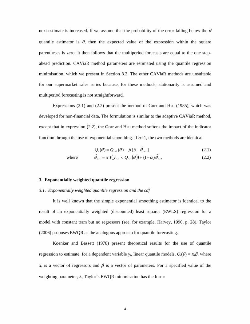
Koenker and Bassett (1978) describe how estimators of different quantiles can be
combined to form a robust estimator of the central location of a distribution. It, therefore,
seems natural to combine the EWQR quantile estimators in a similar way to provide robust
point forecasts. Koenker and Bassett propose the use of Tukey’s (1970) trimean and the
Gastwirth (1966) estimator. Judge et al. (1988) suggest an alternative five-quantile estimator.
We present these estimators in the following expressions:
Trimean: )75.0(ˆ25.0)5.0(ˆ5.0)25.0(ˆ25.0ˆ tttt QQQy ++=
Gastwirth : )(ˆ3.0)5.0(ˆ4.0)(ˆ3.0ˆ 32
31
tttt QQQy ++=
Five-quantile: )9.0(ˆ05.0)75.0(ˆ25.0)5.0(ˆ4.0)25.0(ˆ25.0)1.0(ˆ05.0ˆ tttttt QQQQQy ++++=
A Winsorised estimator involves trimming a dataset of its upper and lower 100α % of
values (Tukey, 1962). In the time series context, all in-sample observations below their
corresponding in-sample fitted EWQR α quantile would be set equal to this value, and all in-
sample observations above their corresponding in-sample fitted EWQR (1- α) quantile would be
set equal to this value. A standard point forecasting method, such as simple exponential
smoothing, would then be applied to the resulting series, with forecasts produced from the
simple exponential smoothing method in the usual way. As each new observation becomes
available, the EWQR estimated α and (1-α) quantiles would be updated, the trimming would be
performed for the new observation, and then the point forecast updated for the next period.
We are not aware of the previous use of any of the estimators described in this section
for univariate forecasting, apart from the EWMM.

9
4. Empirical comparison of point forecasting methods
4.1. Description of the study
In this section, we compare the accuracy of established point forecasting methods
with the EWQR-based robust point forecasting methods discussed in the previous section.
The study used time series of daily observations of sales of different items from an outlet of a
large UK supermarket chain. As greater interest and benefit lies with improved forecasting
for higher volume series, we considered only those series with median daily sales greater or
equal to 5. We felt that none of the forecasting methods that we wished to compare, including
the company’s own method, would be suitable for series that contained a large number of
successive days with zero sales. Therefore, we did not include series that consisted of long
periods of zeros or series that contained only intermittent observations. This resulted in 256
series, which varied in length from 72 to 1436 observations with a median of 764
observations. Figure 2 presents the histogram for the lengths of the series.
---------- Figures 2 to 5 ----------
In Figures 3 to 5, we present summary information for the deseasonalised series using
the same measures and histograms considered by Fildes et al. (1998) for different
deseasonalised data. To deseasonalise the series, we used multiplicative seasonal
decomposition, which is based on ratio-to-moving averages and was used in the M3-
Competition (Makridakis and Hibon, 2000). The histogram in Figure 3 shows that the
correlation between the deseasonalised series and a deterministic linear trend is high for few
of the series. The measure summarised in Figure 4 is the adjusted R2 for the regression of
deseasonalised sales on a deterministic linear trend and autoregressive terms of orders one,
two and three. This is used by Fildes et al. as an approximate measure for the “systematic
variation which can be forecast using simpler methods”. The results in Figure 4 are
consistent with our earlier suggestion that the series are characterised by high volatility.
Figure 5 summarises the proportion of outliers in the series, where an outlier is defined, as in

10
Fildes et al. They define an outlier to be any observation for which the corresponding
observation in the differenced series is outside the inter-quartile range of the differenced
series by a distance that is at least 1.5 times the width of the inter-quartile range.
As we explained in Section 1, the series were characterised by intra-week seasonality
and high volatility, with few displaying trend. Intra-year seasonality is also apparent in some
of the series but, with at most four years of observations for any series, we followed the
practice of the company and did not try to incorporate it in any method.
The company’s outlets are open seven days a week, but not bank holidays. We
replaced bank holidays by the average of the corresponding day of the week from the week
before and the week after the day in question. Using a similar approach, we removed the
Christmas period from the data because the methods considered in this study are not designed
for such unusual periods. This is consistent with the approach taken by the company, as they
do not use their exponential smoothing approach for the Christmas period.
We estimated method parameters using the first 80% of observations in each series.
We used the final 20% for post-sample forecast evaluation. For many of the products in our
dataset, a forecast lead time of 5 to 7 days was of most importance to the company. However,
this varied across the range of products, and so, in consultation with the company, we
considered forecast horizons of one to 14 days in our study. For each series, we rolled the
forecast origin forward through the post-sample evaluation period to produce a collection of
forecasts from each method for each horizon. For the one-day horizon, this resulted in each
method being evaluated on a total of 42,633 post-sample sales observations. We employed
the statistical programming language Gauss for all computational work in this paper.
4.2. Point forecasting methods based on smoothing the level
We included in the study eight methods that involve exponential smoothing of the
level of each series. These methods are listed below. We derived parameter values for all

11
methods, except P2 and P7, by the common procedure of minimising the sum of squared in-
sample one-step-ahead forecast errors, with parameters constrained to lie between zero and
one. We used simple averages of the first few observations to calculate initial values for the
smoothed components (see Williams and Miller, 1999). Using multiplicative seasonal
decomposition, we deseasonalised the data prior to using Methods P1 to P5, as these methods
are appropriate for series with no seasonality. The resultant forecasts were reseasonalised
before comparison with the raw sales data. We also implemented random walk forecasts, but
the results were very poor due to the highly volatile nature of the series.
Method P1. Simple exponential smoothing.
Method P2. Simple exponential smoothing using least absolute deviations (LAD). Gardner
(1999) proposes that the smoothing parameter is optimised by minimising the sum of the
absolute value of the one-step-ahead forecast errors. This has the appeal of robustness, and so
is a useful benchmark for the robust EWQR-based methods, which we present in Section 4.3.
Method P3. Holt’s exponential smoothing.
Method P4. Damped Holt’s exponential smoothing.
Method P5. Brown’s double exponential smoothing.
Method P6. Holt-Winters exponential smoothing for multiplicative seasonality.
Method P7. Company’s method. This involves smoothing the total weekly sales, Wt, and the
split, Lt, of the weekly sales across the days of the week. The parameters are set at the same
subjectively chosen values for all series; α = 0.7 and γ = 0.1.
1
6
0)1( −
=− −+= ∑ t
iitt WyW αα
77
1
)1( −
=−
−+=
∑t
iit
tt L
y
yL γ
γ
The forecasts are given by: 7)(ˆ −+×= mttt LWmy for m = 1 to 7
14)(ˆ −+×= mttt LWmy for m = 8 to 14

12
Method P8. Optimised company’s method. We optimised values for the parameters α and γ.
4.3. Robust point forecasting methods based on EWQR
We implemented the following robust methods, which were described in Section 3.5:
Method P9. Median. This is equivalent to the EWMM approach of Dunsmuir et al. (1996).
Method P10. Trimean.
Method P11. Gastwirth.
Method P12. Five-quantile.
Method P13. Winsorised with α = 0.05. For Methods P13 to P15, simple exponential
smoothing was applied to the Winsorised series. For simplicity, the values of the trimming
percentage, α, were chosen arbitrarily. An alternative is to optimise α based on in-sample fit.
Method P14. Winsorised with α = 0.10.
Method P15. Winsorised with α = 0.25.
For all seven methods, we estimated quantiles using EWQR with a constant and no
regressors. As this approach clearly cannot capture seasonality, we deseasonalised the data
prior to using EWQR. Apart from the appeal of simplicity, we opted for the use of only a
constant term in the EWQR because, as we show in Section 5, it led to better quantile
forecasts, for our data, than those produced by EWQR with regressors.
For the series with fewer than 364 observations (one year of data) in the estimation
sample, we performed EWQR with the whole estimation sample. For the series with at least
364 observations, we used a moving window of just the most recent 364 observations. This
saved computational running time, without noticeably affecting quantile forecast accuracy. In
Section 3.1, we commented that the method of Boudoukh et al. (1998) is the same as EWQR
with just a constant term. They also used a moving window of the most recent year of
observations, which for their finance application amounted to 250 trading days.
13
Optimisation of the weighting parameter λ, in the EWQR minimisation of expression
(3.1), proceeded by the use of a rolling window of 364 observations to estimate one step-
ahead quantile forecasts for each of the remaining observations in the estimation sample. The
value of λ deemed to be optimal was the value that produced one-step-ahead quantile
forecasts leading to the minimum value of the summation in the standard quantile regression
minimisation (QR Sum), which is given in expression (4.1). We computed this summation
over a grid of values for λ between 0.7 and 1, with a step size of 0.005. We performed the
optimisation separately for each of the different values of θ (i.e. for each different quantile).
We did not perform the optimisation for series for which there were fewer than 548
(=364+182) observations in the estimation sample. We felt that 182 observations (six months
of data) was a reasonable minimum from which to evaluate the in-sample quantile forecasts.
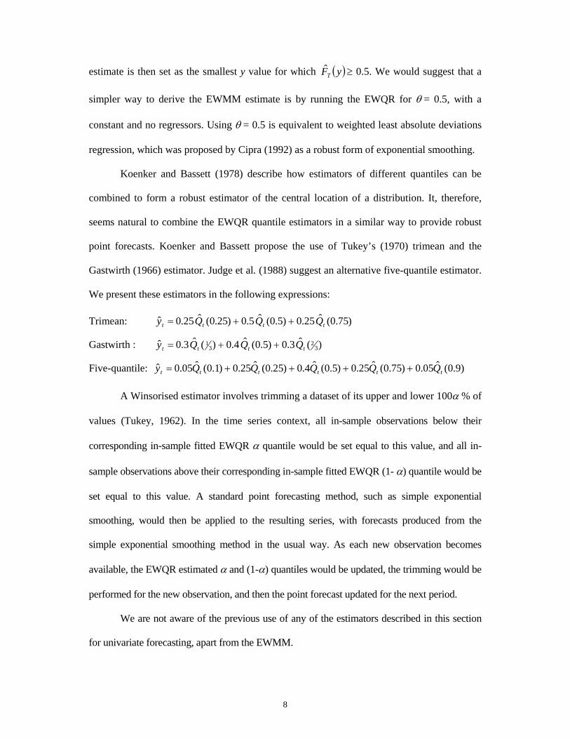
QR Sum = ( )( )( )
∑ ∑≥ <
−−+−θ θ
θθθθtt ttQy|t Qy|t
tttt QyQy )(1)( (4.1)
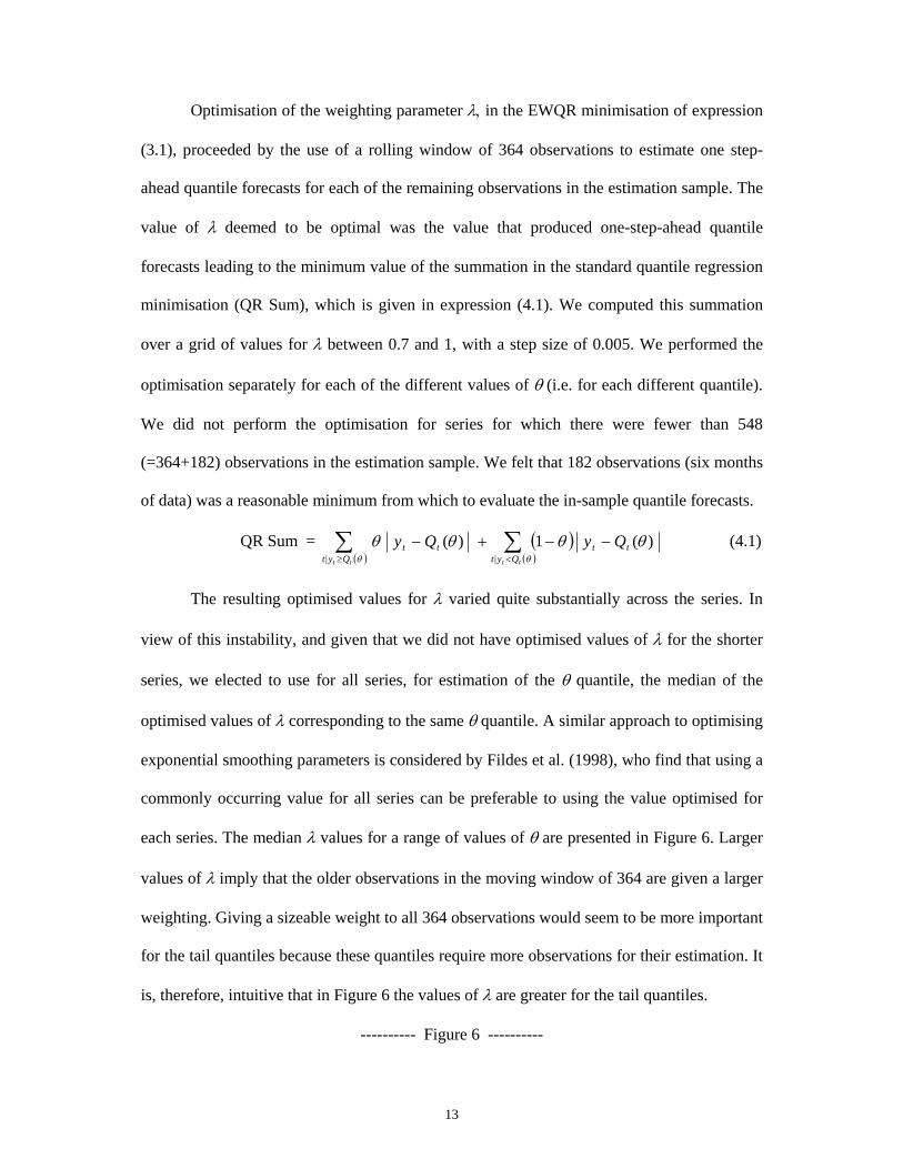
The resulting optimised values for λ varied quite substantially across the series. In
view of this instability, and given that we did not have optimised values of λ for the shorter
series, we elected to use for all series, for estimation of the θ quantile, the median of the
optimised values of λ corresponding to the same θ quantile. A similar approach to optimising
exponential smoothing parameters is considered by Fildes et al. (1998), who find that using a
commonly occurring value for all series can be preferable to using the value optimised for
each series. The median λ values for a range of values of θ are presented in Figure 6. Larger
values of λ imply that the older observations in the moving window of 364 are given a larger
weighting. Giving a sizeable weight to all 364 observations would seem to be more important
for the tail quantiles because these quantiles require more observations for their estimation. It
is, therefore, intuitive that in Figure 6 the values of λ are greater for the tail quantiles.
---------- Figure 6 ----------

14
4.4. Point forecasting results
We evaluated post-sample forecasting performance at each forecast horizon for each
series using the mean absolute error (MAE) and the root mean squared error (RMSE). Since
the order of magnitude of the forecast errors varied across the series, it was not appropriate to
average the error measures across the 256 series. Percentage error measures can be averaged,
but using a percentage error measure is not recommended when the value of the series can be
close to zero, which was often the case for our sales data. In order to summarise performance
across all the series, we calculated a measure of average performance relative to simple
exponential smoothing. For the MAE results, the calculation proceeded by computing, for each
series and each forecast horizon, the ratio of the MAE for that method to the MAE for simple
exponential smoothing, Method P1. We then calculated the weighted geometric mean of this
measure across the 256 series, where the weighting was proportional to the number of post-
sample observations in each series. Expression (4.2) presents the measure:
1001256
1
256
11 ×
⎟⎟⎟⎟⎟⎟
⎠
⎞
⎜⎜⎜⎜⎜⎜
⎝
⎛
−∑⎟⎟⎠
⎞⎜⎜⎝
⎛⎟⎟⎟⎟⎟⎟
⎠
⎞
⎜⎜⎜⎜⎜⎜
⎝
⎛
==∏ j
j
i
N
N
iPi
i
MAEMAE (4.2)
where MAEi and 1PiMAE are the MAE for the method being considered and for Method P1,
respectively; and Ni is the number of post-sample observations for series i. Lower values of
the measure are better, with negative values indicating that the method outperforms Method P1.
For conciseness, Table 1 reports the average of the accuracy measure for pairs of forecast
horizons. The values in bold highlight the best performing method at each horizon. The final
column of the table presents the average of the accuracy measure across the 14 horizons. We
also calculated the relative measure using RMSE instead of MAE in expression (4.2), but we
do not report the results in detail here because they were similar to those in Table 1.
---------- Table 1 ----------
15
Let us first consider the results in Table 1 for the standard point forecasting methods,
Methods P1 to P6. Perhaps of greatest surprise is the poor performance of the multiplicative
Holt-Winters method. This is likely to be due to the unstable ratios that result within the
method when the time series takes values close to or equal to zero. The superior results for
Methods P1 to P5 indicate that multiplicative seasonal decomposition is a more robust
approach to handling the seasonality. We elected not to implement the additive version of
Holt-Winters because our belief was that the seasonality was not additive. This view is
supported by the choice of multiplicative seasonal modelling within the company’s method.
Comparing the results for Methods P1 and P2 indicates that there is no gain in using LAD to
optimise the simple exponential parameter. The fact that simple exponential smoothing was
more accurate than Holt’s, damped Holt’s and Brown’s supports our earlier comment that
few of the sales series contain trend.
Comparing the results for Methods P7 and P8 shows that optimising the parameters in
the company’s method provides a clear improvement over the company’s subjective choice
of parameters. This finding is consistent with the literature on exponential smoothing
methods (e.g. Fildes et al. 1998). The company’s method with optimised parameters, Method
P8, performs well for the early lead times, but the positive value in the final column of the
table shows that, overall, it is outperformed by simple exponential smoothing, Method P1.
Turning to the methods based on EWQR, Methods P9 to P15, we see from the final
column in Table 1 that overall they all outperformed all the level smoothing methods,
Methods P1 to P8. The best results were achieved using the Winsorised approach with
trimming α set at 25%, which implies trimming of all observations outside the interquartile
range. Table 2 aims to provide a little more insight into the results. It shows the percentage of
the 256 series for which the MAE for this method is lower than the MAE for the optimised
company’s method. The Winsorised method can be seen to dominate beyond the early horizons.
---------- Tables 2 and 3 ----------

16
In Section 4.1, we commented that the 256 series vary in length quite considerably. In
order to establish whether the relative performances of the methods depends on the length of the
series, we calculated the relative percentage measure separately for the following four categories
of series lengths: fewer than one year of observations, between one and two years of
observations, between two and three years, and more than three years. Table 3 provides the
results for the optimised company’s method and the EWQR-based Winsorised approach with
trimming α set at 25%. The only noticeable difference in the rankings of the two methods across
the four categories is for one and two day-ahead prediction, where the EWQR-based method
seems to be slightly preferable for the shorter series and a little worse for the longer series.
5. Empirical comparison of quantile forecasting methods
5.1. Description of the study
In this section, we compare methods for forecasting the following four quantiles:
0.025, 0.25, 0.75 and 0.975. As in Section 4, we compare post-sample forecasts for lead
times from one to 14 days for the final 20% of observations in each of the 256 sales series.
We deseasonalised the data prior to forecasting with all the methods, except Method Q7.
5.2. Quantile forecasting methods based on a point forecast
Of the standard point forecasting methods in Section 4, the method that overall was the
most accurate was simple exponential smoothing. In view of this, we constructed quantile
forecasts as the simple exponential smoothing point forecast plus the quantile of the forecast
error distribution estimated using the following two different approaches:
Method Q1. Empirical. For each lead time, we used the distribution of the forecast errors, for
that lead time, in a moving window of the most recent 364 periods.
Method Q2. Theoretical variance. We used a Gaussian assumption with the simple exponential
smoothing multi step-ahead theoretical error variance formula:

17
( ) ( )( )22 11)(ˆvar ασ −+=− − kkyy ektt
where )(ˆ ky kt − is the k step-ahead forecast; 2eσ is the one step-ahead variance calculated
from a moving window of the most recent 364 days; and α is the smoothing parameter.
5.3. Adaptive quantile forecasting methods
We implemented the adaptive CAViaR method and the method of Gorr and Hsu (1985),
which we presented in Section 2. For both methods, multiperiod forecasts are identical to the
one day-ahead prediction. We performed parameter optimisation for each method.
Method Q3. Adaptive CAViaR.
Method Q4. Gorr and Hsu.
5.4. Quantile forecasting methods based on EWQR
We considered the following three different versions of the EWQR approach:
Method Q5. EWQR with a constant and no regressors.
Method Q6. EWQR with a constant and a linear trend term.
Method Q7. EWQR with a constant and the sinusoidal seasonal terms in expression (5.1). The
bi are constant parameters, and d(t) is a repeating step function that numbers the days of the
week from 1 to 7. Preliminary analysis for our data indicated that two sine and two cosine
terms was preferable to one or three.
( ) ( ) ( ) ( )7)(
47)(
37)(
27)(
1 4cos4sin2cos2sin tdtdtdtd bbbb ππππ +++ (5.1)
We also considered the damped trend formulation of expression (3.6). However, the
median value of the optimised damping parameter was one, which implied no damping. We
suspect that this is due to there being trend in few of the series.
We implemented the three EWQR methods in the same way as described for our
point forecasting study of Section 4. The median optimised values of λ for the four quantiles

18
are presented for the three methods in Table 4. It is interesting to see that the values of λ are
higher for the EWQR implementations that included regressors. The implication of this is
that giving a sizeable weight to all 364 observations is more important when regressors are
included. This is intuitive because it indicates that fitting regressors requires more
information than simply fitting a constant term. Note that, although a λ value of 0.995 may
seem high, it does result in noticeable discounting over a reasonable size window. For
example, over a four-week period, the weight reduces to 0.99528=0.869, and over a one-year
period, the weight reduces to 0.995364=0.161.
---------- Table 4 ----------
5.5. Quantile forecasting results
The unconditional coverage of a θ quantile estimator is the percentage of
observations falling below the estimator. Ideally, the percentage should be θ. To summarise
unconditional coverage across the four quantiles, we calculated chi-squared goodness of fit
statistics for each method, at each lead time, for each of the 256 series. We calculated the
statistic for the total number of post-sample observations falling within the following five
categories: below the 0.025 quantile estimator, between each successive pair of quantile
estimators, and above the 0.975 quantile estimator. Assuming independence of the resulting
chi-squared statistics for the different series, we then summed these statistics for all the 256
series. The only two of the resulting summed chi-squared statistics that were not significant,
at the 5% level, were those for one day-ahead prediction from the two adaptive quantile
modelling methods, Methods Q3 and Q4. The chi-squared statistics, from different lead times
for the same method, are not independent. Therefore, statistical testing would be invalid if
these statistics were summed or averaged. Nevertheless, for conciseness, Table 5 reports the
average of the chi-squared statistics for pairs of forecast horizons, and the average across the
14 horizons. Lower values of the measure are better.

19
---------- Table 5 ----------
Table 5 shows that the best performing method at all lead times is the adaptive
CAViaR method. The fact that it outperforms the Gorr and Hsu method suggests that the
smoothing in expression (2.2) of the Gorr and Hsu method is not beneficial. The use of
EWQR with a constant but no regressors, Method Q5, also performed well. By contrast, the
results are very poor for the EWQR method with trend or seasonal terms. As we have already
discussed, few of the supermarket series contain trend, so we should not have expected
benefit in including the trend term. The poor results in Section 4 for the Holt-Winters method
indicated that modelling seasonality was difficult for this data, and that seasonal
decomposition prior to modelling was preferable. The same seems to be the case with regard
to the use of the EWQR method.
Testing for unconditional coverage is insufficient, as it does not assess the dynamic
properties of each quantile estimator (Christoffersen, 1998). The essence of tests of
conditional coverage is to examine whether there is autocorrelation in the hit variable,
defined as ( ) θθ −≤= )(ˆttt QyIHit . Unfortunately, when evaluating tail quantiles, the hit
variable can sometimes contain no variation, in which case the test cannot be performed. For
our 256 supermarket series, this was frequently the case for one or more of the seven
methods. A formal testing of conditional coverage was, therefore, not possible. Instead, we
evaluated the dynamic properties of the methods using the QR Sum, which is presented in
expression (4.1). This measure can be viewed as the equivalent of the MAE and RMSE for
evaluating quantile forecast accuracy. It is one of the measures reported by Engle and
Manganelli (2004) in their VaR study. We calculated the post-sample QR Sum for each
method applied to each series at each forecast horizon. Replacing the MAE terms in
expression (4.2) by the QR Sum, we then computed the relative percentage measure, with the
QR Sum for the Empirical method, Method Q1, in the denominator of the expression. Lower

20
values of the measure are better, with negative values indicating that the method
outperformed Method Q1.
Using the relative QR Sum measure, overall, the relative performance of the methods
was similar to that in Table 5 for the chi-squared statistic. Tables 6 and 7 report the results
for the 0.025 and 0.975 quantiles. It seems sensible to focus on the three methods that
performed reasonably in Table 5: adaptive CAViaR, Gorr and Hsu and EWQR with a
constant and no regressors. The results in Tables 6 and 7 show that, of these three methods,
the EWQR method has the best dynamic properties for both quantiles at all lead times.
---------- Tables 6 and 7 ----------
6. Summary and concluding comments
The daily sales series considered in this paper are characterised by high volatility and
skewness, which are both time-varying. In addition, the series have occasional outlying
observations. These features motivate consideration of point and interval forecasting methods
that are robust with regard to distributional assumptions. As predictions are required for
many different items, the method must be suited to implementation within an automated
procedure. Our proposal is to generate point and interval forecasts from quantile forecasts
generated using EWQR. We have shown that this can be viewed as simple exponential
smoothing of the cdf. The EWQR framework has several benefits. First, it enables efficient
solution through the use of linear programming. Second, it allows regressors, such as a trend
and seasonal terms, to be included in the quantile model. Third, the regression framework
provides scope for statistical inference.
For the sales series, the quantile forecasts from EWQR with only a constant term
compared favourably with a variety of other methods. Another method that performed well
was the adaptive CAViaR method, which has previously only been applied to financial data.

21
Including trend or seasonal terms in the EWQR led to poor results, which motivates further
experimentation with trending and seasonal series.
Poor accuracy resulted from quantile forecasts based on a Gaussian distribution
centred at the simple exponential smoothing point forecast with variance calculated using the
theoretical error variance formula. This suggests that the statistical models underlying the
standard exponential smoothing methods are not well suited to this data. Indeed, point
forecasts from these standard methods, as well as the company’s own approach, were
outperformed by robust point forecasting methods based on the EWQR quantile forecasts.
Acknowledgements
We are grateful to the members of the sales forecasting group at the collaborating
company, and in particular Jon Tasker. We also acknowledge the very helpful comments of
Jan De Gooijer and Everette Gardner on an earlier version of this paper. We are also grateful
for the helpful comments of two anonymous referees.
References
Boudoukh, J., Richardson, M., Whitelaw, R.F., 1998. The best of both worlds, Risk 11 May 64-
67.
Chatfield, C., 1993. Calculating interval forecasts, Journal of Business and Economic Statistics
11 121-135.
Christoffersen, P.F., 1998. Evaluating interval forecasts, International Economic Review 39
841-862.
Cipra, T., 1992. Robust exponential smoothing, Journal of Forecasting 11 57-69.
Dunsmuir, W.T.M., Scott, D.J., Qiu, W., 1996. The distribution of the weighted moving
median of a sequence of iid observations, Communications in Statistics: Simulation and
Computation 25 1015-1029.

22
Engle, R.F., Manganelli, S., 2004. CAViaR: Conditional autoregressive value at risk by
regression quantiles, Journal of Business and Economic Statistics 22 367-381.
Fildes, R., Hibon, M., Makridakis, S., Meade, N., 1998. Generalising about univariate
forecasting methods: Further empirical evidence, International Journal of Forecasting 14 339-
358.
Gardner, E.S., Jr., 1985. Exponential smoothing: the state of the art, Journal of Forecasting 4 1-
28.
Gardner, E.S., Jr., 1988. A simple method of computing prediction intervals for time-series
forecasts, Management Science 34 541-546.
Gardner, E.S., Jr., 1999. Note: Rule-based forecasting vs. damped trend exponential smoothing,
Management Science 45 1169-1176.
Gardner, E.S., Jr., McKenzie, E., 1985. Forecasting trends in time series, Management Science
31 1237-1246.
Gastwirth, J.L., 1966. On robust procedures, Journal of the American Statistical Association 61
929-948.
Gorr, W.L., Hsu, C., 1985. An adaptive filtering procedure for estimating regression quantiles,
Management Science 31 1019-1029.
Harvey, A.C., 1990. Forecasting, Structural Time Series Models and the Kalman Filter,
Cambridge University Press, New York.
Hyndman, R.J., Koehler, A.B., Ord, J.K., Snyder, R.D., 2005. Prediction intervals for
exponential smoothing using two new classes of state space models, Journal of Forecasting 24
17-37.
Judge, G.G., Hill, R.C., Griffiths, W.E., Lütkepohl, H., Lee, T.-C., 1988. Introduction to the
Theory and Practice of Econometrics, Wiley, New York.
Koenker, R.W., Bassett, G.W., 1978. Regression quantiles, Econometrica 46 33-50.

23
Makridakis, S., Hibon, M., 2000. The M3-Competition: results, conclusions and implications,
International Journal of Forecasting 16 451-476.
Taylor, J.W., 2006. Estimating value at risk using exponentially weighted quantile regression,
Working Paper, University of Oxford.
Taylor, J.W., Bunn, D.W., 1999. A quantile regression approach to generating prediction
intervals, Management Science 45 225-237.
Tukey, J.W., 1962. The future of data analysis, Annals of Mathematical Statistics 33 1-67.
Tukey, J.W., 1970. Explanatory Data Analysis, Addison-Wesley, Reading, MA.
Williams, D.W., Miller, D., 1999. Level-adjusted exponential smoothing for modeling
planned discontinuities, International Journal of Forecasting 15 273-289.

24
Figure 1 Daily supermarket sales of a single item.
Figure 2 Histogram for number of observations in the daily supermarket sales series.
0
5
10
15
20
25
30
35
40
0 182 364 546 728 910 1092days
sales
0
5
10
15
20
25
30
35
40
72 to
200
201
to 4
00
401
to 6
00
601
to 8
00
801
to10
00
1001
to12
00
1201
to14
00
1401
to14
36
Number of observations
Frequency (%)

25
Figure 3 Histogram for strength of deterministic linear trend in the daily supermarket sales series.
Figure 4 Histogram for variation explained by deterministic linear trend and AR terms
in the daily supermarket sales series. Figure 5 Histogram for proportion of outlying observations in the daily supermarket
sales series.
0
5
10
15
20
25
30
35
0 to
1
1 to
2
2 to
3
3 to
4
4 to
5
5 to
6
6 to
7
7 to
8
8 to
9
9 to
10
10 to
11
11 to
12
12 to
13
Proportion of outlying observations (%)
Frequency (%)
02468
10121416
-0.8
to -0
.7
-0.7
to -0
.6
-0.6
to -0
.5
-0.5
to -0
.4
-0.4
to -0
.3
-0.3
to -0
.2
-0.2
to -0
.1
-0.1
to 0
0 to
0.1
0.1
to 0
.2
0.2
to 0
.3
0.3
to 0
.4
0.4
to 0
.5
0.5
to 0
.6
0.6
to 0
.7
Correlation with deterministic linear trend
Frequency (%)
0
5
10
15
20
25
30
-5 to
0
0 to
5
5 to
10
10 to
15
15 to
20
20 to
25
25 to
30
30 to
35
35 to
40
40 to
45
45 to
50
50 to
55
55 to
60
60 to
65
65 to
70
70 to
75
Adjusted R2 (%)
Frequency (%)

26
Figure 6 Median of the optimised values of the weighting parameter, λ, for the exponentially weighted θ quantile regression of expression (3.1).
Table 1 Evaluation of point forecasting methods using the relative MAE measure of
expression (4.2), calculated for all 256 series. Accuracy measured relative to Method P1. Lower values are better.
Forecast Horizon 1-2 3-4 5-6 7-8 9-10 11-12 13-14 All
Level Smoothing Methods
P1. Simple 0.0 0.0 0.0 0.0 0.0 0.0 0.0 0.0
P2. Simple using LAD 0.7 0.6 0.7 0.6 0.5 0.5 0.6 0.6
P3. Holt’s 0.8 1.1 1.2 1.7 2.5 2.9 3.2 1.9
P4. Damped Holt’s 0.7 0.7 0.7 0.7 0.7 0.7 0.6 0.7
P5. Brown’s 1.4 2.2 2.9 4.1 5.5 6.6 7.7 4.4
P6. Holt-Winters’ 4.7 4.7 5.3 6.4 7.0 7.4 8.1 6.2
P7. Company -0.7 -1.6 -0.6 1.8 3.3 4.0 5.4 1.7
P8. Optimised Company -1.9 -2.4 -1.3 0.7 1.6 2.4 3.6 0.4
EWQR Methods
P9. Median -1.0 -1.5 -1.1 -1.0 -1.8 -1.8 -1.4 -1.4
P10. Trimean -1.2 -1.8 -1.3 -1.4 -2.1 -2.1 -1.8 -1.7
P11. Gastwirth -1.3 -1.8 -1.4 -1.4 -2.1 -2.1 -1.8 -1.7
P12. Five Quantile -1.0 -1.5 -1.1 -1.2 -2.0 -2.0 -1.7 -1.5
P13. Winsorised α = 0.05 -0.9 -1.1 -1.0 -1.0 -1.2 -1.1 -1.1 -1.0
P14. Winsorised α = 0.10 -1.2 -1.5 -1.3 -1.3 -1.6 -1.5 -1.4 -1.4
P15. Winsorised α = 0.25 -1.6 -2.0 -1.6 -1.7 -2.3 -2.1 -1.9 -1.9
0.90
0.92
0.94
0.96
0.98
1.00
0.0 0.2 0.4 0.6 0.8 1.0θ
Median λ

27
Table 2 Percentage of the 256 series for which the MAE for the EWQR-based
Winsorised Method P15 with α=0.25 is lower than the MAE for the optimised company’s Method P8. Bold indicates significantly greater than 50% at the 5% significance level.
Forecast Horizon 1 2 3 4 5 6 7 8 9 10 11 12 13 14
% 50 49 49 54 54 55 60 74 75 75 73 76 76 78 Table 3 Evaluation of point forecasting Methods P8 and P15 using the relative MAE
measure of expression (4.2), calculated for series of different lengths. Accuracy measured relative to Method P1. Lower values are better.
Forecast Horizon 1-2 3-4 5-6 7-8 9-10 11-12 13-14 All
83 series with observations ≤ 364 P8. Optimised Company -2.5 -2.7 -2.4 0.6 2.5 3.2 4.5 0.5
P15. EWQR Winsorised α = 0.25 -2.6 -2.1 -2.1 -2.2 -2.6 -2.3 -1.7 -2.2
39 series with 365 ≤ observations ≤ 728 P8. Optimised Company -1.2 -1.3 -0.7 1.5 2.2 2.6 3.4 0.9
P15. EWQR Winsorised α = 0.25 -1.6 -1.8 -1.5 -1.4 -2.0 -2.0 -2.0 -1.7
28 series with 729 ≤ observations ≤ 1092 P8. Optimised Company -1.6 -2.0 -1.4 0.4 1.8 2.4 3.8 0.5
P15. EWQR Winsorised α = 0.25 -0.9 -1.0 -0.9 -0.9 -1.0 -0.9 -0.9 -0.9
106 series with 1093 ≤ observations ≤ 1436 P8. Optimised Company -2.0 -2.6 -1.2 0.6 1.5 2.3 3.6 0.3
P15. EWQR Winsorised α = 0.25 -1.6 -2.2 -1.7 -1.8 -2.5 -2.3 -2.1 -2.1
All 256 series
P8. Optimised Company -1.9 -2.4 -1.3 0.7 1.6 2.4 3.6 0.4
P15. EWQR Winsorised α = 0.25 -1.6 -2.0 -1.6 -1.7 -2.3 -2.1 -1.9 -1.9

28
Table 4 Median of the optimised values of the weighting parameter, λ, for three
different versions of the exponentially weighted θ quantile regression of expression (3.1).
θ 0.025 0.25 0.75 0.975
Q5. EWQR no regressors 0.990 0.950 0.925 0.9725
Q6. EWQR trend 0.995 0.985 0.970 0.995
Q7. EWQR seasonal 0.995 0.990 0.980 0.995
Table 5 Evaluation of quantile forecasting methods using unconditional coverage chi-
square statistic summarising performance across all four quantiles. Lower values are better.
Forecast horizon 1-2 3-4 5-6 7-8 9-10 11-12 13-14 All
Methods Based on a Point Forecast
Q1. Empirical 2459 2648 2734 2952 3267 3489 3797 3049
Q2. Theoretical variance 4142 4360 4540 4666 4902 5128 5420 4737
Adaptive Methods
Q3. Adaptive CAViaR 1018 1371 1587 1822 2073 2413 2744 1861 Q4. Gorr and Hsu 1193 1537 1712 1956 2163 2474 2804 1977
EWQR Methods
Q5. EWQR no regressors 1528 1708 1907 2156 2505 2812 3136 2250
Q6. EWQR trend 3609 4249 4902 5720 6690 7572 8471 5888
Q7. EWQR seasonal 3145 3124 3222 3492 3820 3890 3938 3519

29
Table 6 Evaluation of 0.025 quantile forecasts using relative QR Sum measure.
Accuracy measured relative to Method Q1. Lower values are better. Forecast horizon 1-2 3-4 5-6 7-8 9-10 11-12 13-14 All
Methods Based on a Point Forecast
Q1. Empirical 0.0 0.0 0.0 0.0 0.0 0.0 0.0 0.0
Q2. Theoretical variance 2.7 2.0 1.4 0.9 0.0 -0.1 0.0 1.0
Adaptive Methods
Q3. Adaptive CAViaR -20.1 -22.0 -23.5 -24.8 -26.6 -27.4 -28.0 -24.6
Q4. Gorr and Hsu -19.6 -21.5 -23.0 -24.4 -26.1 -26.9 -27.4 -24.1
EWQR Methods
Q5. EWQR no regressors -21.1 -23.0 -24.5 -25.8 -27.6 -28.4 -28.9 -25.6 Q6. EWQR trend -19.4 -20.9 -22.1 -23.3 -24.7 -25.3 -25.7 -23.0
Q7. EWQR seasonal -18.4 -20.6 -22.3 -23.6 -25.2 -26.1 -26.7 -23.3 Table 7 Evaluation of 0.975 quantile forecasts using relative QR Sum measure.
Accuracy measured relative to Method Q1. Lower values are better. Forecast horizon 1-2 3-4 5-6 7-8 9-10 11-12 13-14 All
Methods Based on a Point Forecast
Q1. Empirical 0.0 0.0 0.0 0.0 0.0 0.0 0.0 0.0
Q2. Theoretical variance -0.1 -0.1 -0.3 -0.4 -0.5 -0.8 -1.1 -0.5
Adaptive Methods
Q3. Adaptive CAViaR 10.6 9.6 9.8 9.8 9.5 9.2 9.6 9.7
Q4. Gorr and Hsu 11.0 10.1 10.3 10.3 9.9 9.6 9.9 10.2
EWQR Methods
Q5. EWQR no regressors 5.0 4.7 5.3 5.6 5.6 5.7 6.1 5.4
Q6. EWQR trend 13.0 13.2 14.6 15.3 15.3 15.8 16.6 14.8
Q7. EWQR seasonal 11.5 8.9 8.3 8.2 7.1 5.4 4.5 7.7


