HAL Id: tel-01480290https://tel.archives-ouvertes.fr/tel-01480290

Submitted on 1 Mar 2017

HAL is a multi-disciplinary open accessarchive for the deposit and dissemination of sci-entific research documents, whether they are pub-lished or not. The documents may come fromteaching and research institutions in France orabroad, or from public or private research centers.

L’archive ouverte pluridisciplinaire HAL, estdestinée au dépôt et à la diffusion de documentsscientifiques de niveau recherche, publiés ou non,émanant des établissements d’enseignement et derecherche français ou étrangers, des laboratoirespublics ou privés.

Formation of supermassive black holesMélanie Habouzit

To cite this version:Mélanie Habouzit. Formation of supermassive black holes. Astrophysics [astro-ph]. Université Pierreet Marie Curie - Paris VI, 2016. English. NNT : 2016PA066360. tel-01480290

THÈSE DE DOCTORATDE L’UNIVERSITÉ PIERRE ET MARIE CURIE

Spécialité Astrophysique

École Doctorale d’Astronomie & d’Astrophysique d’Ile-de-France

réalisée

à l’Institut d’Astrophysique de Paris

présentée par

Mélanie Habouzit

pour obtenir le grade de

DOCTEUR DE L’UNIVERSITÉ PIERRE ET MARIE CURIE

Sujet de la thèse :

Formation of supermassive black holes

soutenue le 15 septembre 2016

devant le jury composé de :

Benoit Semelin Président du juryMarta Volonteri Directeur de thèseRachel Somerville RapporteurSadegh Khochfar RapporteurRaffaella Schneider ExaminateurJenny Greene ExaminateurYohan Dubois Examinateur

A mon petit Fanfan, mes parents et mes grand-parents.

Abstract

Supermassive black holes (BHs) harboured in the center of galaxies have been confirmed withthe discovery of Sagittarius A? in the center of our galaxy, the Milky Way. Recent surveysindicate that BHs of millions of solar masses are common in most local galaxies, but also thatsome local galaxies could be lacking BHs (e.g. NGC 205, M33), or at least hosting low-massBHs of few thousands solar masses. Conversely, massive BHs under their most luminous formare called quasars, and their luminosity can be up to hundred times the luminosity of an entiregalaxy. We observe these quasars in the very early Universe, less than a billion years after the BigBang, with masses as large as 108 M (Fan et al., 2006b ; Mortlock et al., 2011). BH formationmodels therefore need to explain both the low-mass BHs that are observed in low-mass galaxiestoday, but also the prodigious quasars we see in the early Universe. Several correlations betweenBH mass and galaxy properties have been derived empirically, such as the BH mass-velocitydispersion relation, they may be seen as evidence of BH and galaxy co-evolution through cosmictime. Moreover, BHs impact their host galaxies and vice versa. For example, BH growth isregulated by the ability of galaxies to funnel gas towards them, while BHs are thought to exertpowerful feedback on their host galaxies. BHs are a key element of galaxy evolution, and thereforein order to study BH formation in the context of galaxy evolution, we have used cosmologicalhydrodynamical simulations. Cosmological simulations offer the advantage of following in timethe evolution of galaxies, and the processes related to them, such as star formation, metalenrichment, feedback of supernovae and BHs.

BH formation is still puzzling today, and many questions need to be addressed: How areBHs created in the early Universe? What is their initial mass? How many BHs grow efficiently?What is the occurrence of BH formation in high redshift galaxies? What is the minimum galaxymass to host a BH? Most of these questions are summarized in Fig 1, which represents a sampleof local galaxies with their BHs, in blue points. The red shaded area represent the challenge ofthis thesis, which is to understand the assembly of BHs at high redshift and their properties. MyPhD focuses on three main BH formation models. Massive first stars (PopIII stars) in mini-halos,at redshift z = 20− 30 are predicted to collapse and form a BH retaining half the mass of thestar, . 102 M (Madau & Rees, 2001 ; Volonteri, Haardt & Madau, 2003). This is the Pop IIIstar remnants model. Compact stellar clusters are also thought to be able to collapse and form avery massive star by stellar collisions, which can lead to the formation of a ∼ 103 M BH seed(Omukai, Schneider & Haiman, 2008 ; Devecchi & Volonteri, 2009 ; Regan & Haehnelt, 2009b).Finally, in the direct collapse model, metal-free halos, without efficient coolants (i.e. no metals,no molecular hydrogen), at z = 10 and later, can collapse and form a star-like supermassiveobject, which can collapse into a BH of 104 − 106 M (Bromm & Loeb, 2003 ; Spaans & Silk,2006 ; Dijkstra et al., 2008).

As we will see in this thesis, we have investigated both the BH population in normal localgalaxies, as well as the feasibility of BH formation model to explain the assembly of the highredshift quasar population. First of all, in order to fully understand the population of BHs we

i

ii

Fig. 1 – Sample of BHs in local galaxies in light and dark blue points. BH masses range from few 104 Mto 1010 M. The shaded area represent the domain of BH mass at their formation time, in the earlyUniverse.

observe in low-mass galaxies, we need a theoretical model able to predict the occupation fractionof BHs in low-mass galaxies, and the properties of both these BHs and their host galaxies. Wehave implemented a model accounting for the PopIII remnant and stellar cluster models, inthe numerical code Ramses. We form BHs according to the theoretical models, and let theseBHs evolve with time. So far, cosmological simulations were only used to reproduce the quasarsluminosity function and study their feedback, simulations were therefore seeding BHs by placing a105 M BH in the center of massive galaxies. Our approach allows instead to study BH formation,and to cover the low-mass end of BHs. We then compare the simulated BHs to two differentobservational samples, local galaxies (Reines & Volonteri, 2015), and Lyman-Break Analogs (Jiaet al., 2011a). Local low-mass galaxies are among the most pristine galaxies, because they havea quieter merger history. Therefore BHs in low-mass galaxies, are also thought to be pristine,and to not have evolved much from their birth, thus they can provide us precious clues on BHformation. Lyman-Break Analogs are galaxies very similar to their high redshift analogs, theLyman-Break Galaxies, comparing our simulated samples to BHs found in these galaxies cantherefore also provide us a promising new laboratory to study BHs in high redshift environment,but much closer to us.

The direct collapse model has been much studied recently, but there is no consensus onthe number of BHs that form through this model yet. The number density of BHs, derived bydifferent studies employing semi-analytic models (Dijkstra, Ferrara & Mesinger, 2014) or hybridsemi-analytic models (Agarwal et al., 2012, 2014) varies on several orders of magnitude. Hybridsemi-analytic models are very appealing because they use spatial information from cosmologicalsimulations. However, only small simulated volumes allow one to achieve the high resolutionsneeded to resolve minihalos, and the early metal enrichment. These small boxes probe withdifficulty the feasibility of the direct collapse BH formation model, lacking statistical validation.Instead, in this thesis, we chose to run simulations with different box sizes and resolutions, thatallow us to test the impact of different processes such as metal enrichment and the impact ofsupernova feedback. The main advantage is also that employing large simulation boxes makes

Abstract iii

possible to test different radiation intensity thresholds to destroy molecular hydrogen, which isof paramount importance for the direct collapse model.

iv Abstract

Remerciements

Nous n’avons pas souvent l’occasion de remercier les personnes qui nous épaulent au quotidien,que ce soit professionnellement ou personnellement, ou bien même les deux. Sans elles, rienn’aurait été possible.

Mes premiers remerciements sont pour Marta, qui m’a fait partager son enthousiasme et sa soifde connaissance, merci pour sa patience et sa pédagogie, et pour m’avoir donné l’opportunité detravailler sur des projets passionnants. Nous avons cherché ensemble à répondre à quelques-unesdes questions sur la formation et la croissance des trous noirs supermassifs, mais il en reste encoredes milliers, et j’espère tout autant d’occasions de travailler de nouveau ensemble.Deux autres chercheurs m’ont particulièrement apporté leur aide durant ma thèse. Je remercieYohan Dubois pour sa disponibilité, pour m’avoir fait découvrir Ramses, et pour avoir réponduaux questions de physique, aussi bien qu’aux questions numériques que je me suis posée pendantces trois années. Je remercie également Muhummad Latif pour m’avoir accompagnée sur leschemins sinueux du modèle direct collapse de formation des trous noirs, ainsi que pour sadisponibilité et ses conseils.J’ai également une pensée pour les chercheurs avec qui j’ai débuté et qui m’ont toujours en-couragée et apporté leur soutien, Claudia Maraston à Portsmouth (ICG), et bien sûr ici à Paris(IAP), Gary Mamon, Joseph Silk, et Sébastien Peirani. Je tiens également à remercier Jacques leBourlot pour son soutien et tous les conseils judicieux qu’il a pu me donner.Bien sûr ma thèse n’aurait pas été la même sans notre grande équipe, je remercie donc égalementPedro Capelo, Andrea Negri, Salvatore Cielo et Alessandro Lupi pour le côté italien, TilmanHartwig pour le côté allemand, et Rebekka Bieri pour le côté suisse de notre équipe.

Merci à Rachel Somerville et Sadegh Khochfar d’avoir accepté d’être les rapporteurs dema thèse et d’avoir passé une partie de leurs vacances d’été à lire mon manuscrit, à RaffaellaSchneider et Jenny Greene d’avoir accepté d’être examinatrices, et finalement Benoit Semelind’avoir accepté de présider le jury de ma thèse. Ce sont des chercheurs exceptionnels et jesuis vraiment fière qu’ils aient accepté de faire partie de mon jury de thèse, merci pour leursuggestions et remarques très constructives sur mon travail.

Pendant trois ans, j’ai eu la chance de travailler également au Palais de la Découverte, dedonner des conférences le week-end, et d’écrire des articles pour la revue Découverte du musée.Je remercie Sébastien Fontaine de m’avoir donné cette chance. J’ai pu discuter avec le grandpublic des nombreuses grandes questions de l’astrophysique, m’émerveiller avec eux de toutes lesréponses que nous avons déjà, rire avec toutes ces personnes de 7 à 77 ans qui viennent découvriret apprendre au musée des sciences de Paris. Je ne peux ici pas citer toutes les personnes que jevoudrais remercier, mais j’ai une pensée particulière pour Marc Goutaudier, Andy Richard, etGaëlle Courty qui m’ont apporté une aide précieuse.

v

vi Abstract

Evidemment je ne pourrais pas achever ma thèse sans remercier l’ensemble des doctorants,pour l’ambiance exceptionnelle qui règne à l’IAP. Je commencerais par les anciens, Alice (et sajoie de vivre communicative), Flavien (parce que nous avons découvert Cyclopatte ensemble),Thomas (qui partage un peu le même humour que moi), Vivien (pour le côté beau gosse de l’IAP),Nicolas (pour le côté plus que cool de l’IAP), Vincent (pour sa robe de chambre d’astrophysicien),Pierre (pour sa joie de vivre), Guillaume D. (pour sa bonne humeur et ses conseils sur lespost-docs), Hayley (pour les "touffes" de galaxies), Guillaume P. et Manuel (pour leurs conseilssur la programmation). Ensuite les doctorants qui sont devenus docteur en même temps quemoi, Julia, Alba, Rebekka, Laura (la plus sportive), Clotilde (pour son petit accent allemandquand elle parle en anglais), Jean-Baptiste (le seul homme de la promotion). Enfin tous les plusjeunes à qui je souhaite une très grande réussite, Tilman, Caterina, Federico, Nicolas, Erwan,Sébastien, Siwei, Céline, Jesse, Tanguy et Florian.

Je remercie particulièrement les drôles de dames du bureau 13. Il y aura eu un nombreabsolument étourdissant de fous rires, de larmes, de moments de désespoir, de moments de joie,de danses, de chansons, et un mariage et demi. Ensemble nous avons vécu bien plus qu’une thèse.Je pense à Rebekka avec qui j’ai partagé tous les stressants meetings du mardi, avec qui nousavons écrit des équations ou des lignes de code Ramses sur un tableau noir, je la remercie pourtous ses encouragements dans les moments difficiles, et pour toute sa joie de vivre et sa folie (cequi inclut des patches beauté dans le bureau, des siestes par terre, faire du yoga et manger desgraines). Je remercie Alba et son sourire du Sud, son amour de la nourriture, je repense à toutesles fois où nous avons dîné ensemble (souvent gratuitement) le soir à l’IAP, sa connaissance dela grammaire française, des musées parisiens, son espoir de m’apprendre les verbes irréguliersen anglais ou m’apprendre à être plus positive. Et finalement Julia, que je connais depuis detrès nombreuses années, et que j’adore depuis le premier jour pour son enthousiasme des travauxpratiques, et plus sérieusement pour son amitié, tous ses conseils, son soutien dans les momentsdifficiles, pour tous les potins que nous avons partagés (≈ 4000, à raison de deux par jour pendant6 ans), et tout autant de fous rires.Je remercie Clément pour tout le soutien qu’il m’a apporté durant ces trois années, et aussi pourtoutes les fois où il a eu l’audace de me contredire, que ce soit pour la signification d’un poèmede Baudelaire dans les jardins du Luxembourg, ou sur le fait que je pourrais ne pas avoir raisonen toutes circonstances, ou encore sur le fait qu’il manquait quelque chose sur mes peintures, ouqu’il faille manger des légumes, ou ne pas inventer de nouveaux mots. Merci aussi pour toutesses histoires abracadabrantes racontées au détour des ruelles de Paris une fois la nuit tombée, etpour son émerveillement de tout, de la philosophie aux documentaires Arte. Et aussi pour safascination des abeilles et des fourmis, et bien sûr sa joie de partager cela avec son entouragependant les pauses café.Merci également à Terry pour son soutien infaillible toutes ces années, spécialement dans lesmoments difficiles.

Pour finir, je suis infiniment reconnaissante à ma grande et belle famille de m’avoir accom-pagnée depuis toutes ces années, et particulièrement d’avoir fait le déplacement pour assister àma soutenance de thèse. Il en faut de la patience pour attendre avec moi le passage des étoilesfilantes, tous les ans, pendant les longues soirées d’été. Et du courage pour braver les obscurschemins de la campagne pour tenter, enfin, d’observer la Voie Lactée. Du courage il en aura falluaussi pour supporter la scientifique que je suis, les feuilles d’équations, de calculs, de schémas,les piles de livres à n’en plus finir, les longues soirées à réfléchir, et à garder la lumière allumée

Remerciements vii

une bonne partie de la nuit.Je suis on ne peut plus reconnaissante à mes grand-parents de m’avoir offert mon petit lieu de

paradis, où le chant des oiseaux se mêle aux parfums des fleurs du jardin, où l’on peut se réveillerà midi et déguster des crêpes pour le dessert, où l’on peut s’amuser en taillant les arbustes dujardin, ou en ramassant des pommes dans le verger. Il serait difficile de dire en quelques mots icitout ce que je dois à mes parents, et à quel point je les remercie, tout leur amour et tout leursoutien depuis mon enfance sont, et seront toujours, une force indispensable. Et finalement jeremercie mon petit Fanfan, qui a bien grandi, pour son intelligence, sa culture, ses blagues, sesfous rires du dimanche, sa bonne humeur, pour son soutien et ses conseils (on se demande parfoisqui est le petit frère et qui est la grande soeur), et surtout notre amour partagé du gâteau auxpetits-beurre.

Paris, septembre 2016.

viii Remerciements

Contents

Abstract iii

Remerciements vii

1 Introduction 11.1 Brief historical introduction . . . . . . . . . . . . . . . . . . . . . . . . . . . . . . 21.2 Structure formation in a homogeneous Universe . . . . . . . . . . . . . . . . . . . 4

1.2.1 The homogeneous Universe . . . . . . . . . . . . . . . . . . . . . . . . . . 41.2.2 Linear growth of perturbations and spherical collapse model . . . . . . . . 6

1.3 Formation of galaxies and first stars . . . . . . . . . . . . . . . . . . . . . . . . . 91.4 Black holes as a key component of galaxies . . . . . . . . . . . . . . . . . . . . . 13

1.4.1 BHs and AGN . . . . . . . . . . . . . . . . . . . . . . . . . . . . . . . . . 131.4.2 Local galaxies . . . . . . . . . . . . . . . . . . . . . . . . . . . . . . . . . . 141.4.3 Population of quasars at z = 6 . . . . . . . . . . . . . . . . . . . . . . . . 19

1.5 Black holes as a key component for galaxy evolution . . . . . . . . . . . . . . . . 201.5.1 Co-evolution between BHs and their host galaxies . . . . . . . . . . . . . 211.5.2 AGN feedback . . . . . . . . . . . . . . . . . . . . . . . . . . . . . . . . . 22

1.6 Black hole growth over cosmic time . . . . . . . . . . . . . . . . . . . . . . . . . . 241.7 Theoretical models for black hole formation in the early Universe . . . . . . . . . 29

1.7.1 Remnants of the first generation of stars . . . . . . . . . . . . . . . . . . . 291.7.2 Compact stellar clusters . . . . . . . . . . . . . . . . . . . . . . . . . . . . 331.7.3 Direct collapse of gas . . . . . . . . . . . . . . . . . . . . . . . . . . . . . . 341.7.4 Other models . . . . . . . . . . . . . . . . . . . . . . . . . . . . . . . . . . 38

1.8 Diagnostics to distinguish between BH formation scenarios . . . . . . . . . . . . 381.9 Organization of the thesis . . . . . . . . . . . . . . . . . . . . . . . . . . . . . . . 43

2 Numerical simulation 452.1 Ramses: a numerical code with adaptive mesh refinement . . . . . . . . . . . . . 46

2.1.1 Adaptive mesh refinement . . . . . . . . . . . . . . . . . . . . . . . . . . . 462.1.2 Initial conditions . . . . . . . . . . . . . . . . . . . . . . . . . . . . . . . . 472.1.3 Adaptive time-stepping . . . . . . . . . . . . . . . . . . . . . . . . . . . . 472.1.4 N -body solver . . . . . . . . . . . . . . . . . . . . . . . . . . . . . . . . . 482.1.5 Hydrodynamical solver . . . . . . . . . . . . . . . . . . . . . . . . . . . . . 51

2.2 Sub-grid physics to study galaxy formation and evolution . . . . . . . . . . . . . 522.2.1 Radiative cooling and photoheating by UV background . . . . . . . . . . 522.2.2 Star formation . . . . . . . . . . . . . . . . . . . . . . . . . . . . . . . . . 532.2.3 Equation-of-state . . . . . . . . . . . . . . . . . . . . . . . . . . . . . . . . 542.2.4 SN feedback and metal enrichment . . . . . . . . . . . . . . . . . . . . . . 542.2.5 BH formation . . . . . . . . . . . . . . . . . . . . . . . . . . . . . . . . . . 56

ix

x Contents

2.2.6 BH accretion . . . . . . . . . . . . . . . . . . . . . . . . . . . . . . . . . . 562.2.7 AGN feedback . . . . . . . . . . . . . . . . . . . . . . . . . . . . . . . . . 57

2.3 Smoothed particle hydrodynamics code Gadget . . . . . . . . . . . . . . . . . . 57

3 Pop III remnants and stellar clusters 593.1 Introduction . . . . . . . . . . . . . . . . . . . . . . . . . . . . . . . . . . . . . . . 603.2 Simulation set up . . . . . . . . . . . . . . . . . . . . . . . . . . . . . . . . . . . . 613.3 Seeding cosmological simulations with BH seeds . . . . . . . . . . . . . . . . . . . 62

3.3.1 Selecting BH formation regions . . . . . . . . . . . . . . . . . . . . . . . . 633.3.2 Computing BH initial masses . . . . . . . . . . . . . . . . . . . . . . . . . 633.3.3 BH growth and AGN feedback . . . . . . . . . . . . . . . . . . . . . . . . 64

3.4 The influence of star formation and metallicity on BH formation . . . . . . . . . 643.5 Black hole mass function and occupation fraction . . . . . . . . . . . . . . . . . . 663.6 Black hole growth regulated by efficient SN feedback . . . . . . . . . . . . . . . . 703.7 Comparisons with a sample of local galaxies, and Lyman-Break Analogs . . . . . 753.8 Conclusions . . . . . . . . . . . . . . . . . . . . . . . . . . . . . . . . . . . . . . . 783.9 Perspectives . . . . . . . . . . . . . . . . . . . . . . . . . . . . . . . . . . . . . . . 79

3.9.1 BH growth in the delayed cooling SN feedback simulation . . . . . . . . . 793.9.2 Need for further comparisons with observations, preparing future observa-

tional missions. . . . . . . . . . . . . . . . . . . . . . . . . . . . . . . . . . 79

4 Direct collapse model 854.1 Introduction . . . . . . . . . . . . . . . . . . . . . . . . . . . . . . . . . . . . . . . 864.2 Simulation set up . . . . . . . . . . . . . . . . . . . . . . . . . . . . . . . . . . . . 894.3 Method . . . . . . . . . . . . . . . . . . . . . . . . . . . . . . . . . . . . . . . . . 924.4 Impact of SN feedback on metallicity and star formation . . . . . . . . . . . . . . 944.5 Number density of direct collapse regions in Chunky . . . . . . . . . . . . . . . . 954.6 Horizon-noAGN simulation: Can DC model explain z = 6 quasars? . . . . . . . . 984.7 Comparison between hydro. simulations and (semi-)analytical models . . . . . . 1014.8 Conclusions . . . . . . . . . . . . . . . . . . . . . . . . . . . . . . . . . . . . . . . 1044.9 Perspectives: Applications of hybrid SAMs . . . . . . . . . . . . . . . . . . . . . 107

5 Black hole formation and growth with primordial non-Gaussianities 1115.1 Introduction on primordial non-Gaussianities . . . . . . . . . . . . . . . . . . . . 112

5.1.1 Primordial bispectrum . . . . . . . . . . . . . . . . . . . . . . . . . . . . . 1135.1.2 Introduction of fNL parameter . . . . . . . . . . . . . . . . . . . . . . . . 1145.1.3 Observational constraints, room for non-Gaussianities at small scales . . . 1165.1.4 Previous work, and the idea of running non-Gaussianities . . . . . . . . . 116

5.2 Halo and galaxy mass functions . . . . . . . . . . . . . . . . . . . . . . . . . . . . 1185.2.1 Numerical methods: from non-Gaussian N -body simulations to galaxy

formation model . . . . . . . . . . . . . . . . . . . . . . . . . . . . . . . . 1185.2.2 Predicted halo mass functions from theory . . . . . . . . . . . . . . . . . . 1205.2.3 Results on halo and galaxy mass function . . . . . . . . . . . . . . . . . . 1215.2.4 Conclusions . . . . . . . . . . . . . . . . . . . . . . . . . . . . . . . . . . . 123

5.3 Reionization history of the Universe . . . . . . . . . . . . . . . . . . . . . . . . . 1245.3.1 Far-UV luminosity function and reionization models . . . . . . . . . . . . 1245.3.2 Fraction of ionized volume of the Universe . . . . . . . . . . . . . . . . . . 1255.3.3 Electron Thomson scattering optical depth . . . . . . . . . . . . . . . . . 126

Contents xi

5.3.4 Conclusions . . . . . . . . . . . . . . . . . . . . . . . . . . . . . . . . . . . 1275.4 BH formation and growth with primordial non-Gaussianities . . . . . . . . . . . 128

5.4.1 BHs formed through direct collapse . . . . . . . . . . . . . . . . . . . . . 1295.4.2 BHs formed from the remnants of the first generation of stars. . . . . . . 1375.4.3 BHs in the most massive halos at z = 6.5 . . . . . . . . . . . . . . . . . . 1385.4.4 Conclusions . . . . . . . . . . . . . . . . . . . . . . . . . . . . . . . . . . . 141

6 Conclusions 145

A Monitorat at Palais de la Découverte 149

List of Figures 155

List of Tables 157

List of Publications 157

References 174

xii Contents

Chapter 1Introduction

In this chapter, after giving a brief introduction of the historical discoveries that lead us to ourmodern conception of the evolution of the Universe, we describe the formation and evolution oflarge-scale structures, from the collapse of dark matter halos to the formation of the first stars,and galaxies. Black holes (BHs) are a key component of galaxies today, most of the local galaxiesindeed host a BH, including our Milky Way. The discovery of quasars, powered by massive BHs,indicates that they were already in place less than 1 Gyr after the Big Bang. Moreover, theseBHs are also thought to play an important role in galaxy evolution, through powerful feedbackprocesses. BHs are therefore a key ingredient of galaxy evolution. However, there is still noconsensus on the formation of BHs. We describe the main theoretical scenarios of BH formationat the end of this chapter, and the main questions that still need to be investigated.

Contents1.1 Brief historical introduction . . . . . . . . . . . . . . . . . . . . . . . . 21.2 Structure formation in a homogeneous Universe . . . . . . . . . . . . 4

1.2.1 The homogeneous Universe . . . . . . . . . . . . . . . . . . . . . . . . . 41.2.2 Linear growth of perturbations and spherical collapse model . . . . . . . 6

1.3 Formation of galaxies and first stars . . . . . . . . . . . . . . . . . . . 91.4 Black holes as a key component of galaxies . . . . . . . . . . . . . . . 13

1.4.1 BHs and AGN . . . . . . . . . . . . . . . . . . . . . . . . . . . . . . . . 131.4.2 Local galaxies . . . . . . . . . . . . . . . . . . . . . . . . . . . . . . . . . 141.4.3 Population of quasars at z = 6 . . . . . . . . . . . . . . . . . . . . . . . 19

1.5 Black holes as a key component for galaxy evolution . . . . . . . . . 201.5.1 Co-evolution between BHs and their host galaxies . . . . . . . . . . . . 211.5.2 AGN feedback . . . . . . . . . . . . . . . . . . . . . . . . . . . . . . . . 22

1.6 Black hole growth over cosmic time . . . . . . . . . . . . . . . . . . . 241.7 Theoretical models for black hole formation in the early Universe . 29

1.7.1 Remnants of the first generation of stars . . . . . . . . . . . . . . . . . . 291.7.2 Compact stellar clusters . . . . . . . . . . . . . . . . . . . . . . . . . . . 331.7.3 Direct collapse of gas . . . . . . . . . . . . . . . . . . . . . . . . . . . . . 341.7.4 Other models . . . . . . . . . . . . . . . . . . . . . . . . . . . . . . . . . 38

1.8 Diagnostics to distinguish between BH formation scenarios . . . . . 381.9 Organization of the thesis . . . . . . . . . . . . . . . . . . . . . . . . . 43

1

2 1.1 Brief historical introduction

1.1 Brief historical introduction

The cosmological framework of galaxy formation and evolution, is the culmination of many dis-coveries over the last centuries. In this brief section, we review the most important developmentsin our knowledge of the Universe, and their implications.Starting in 1771, the French observer Messier, referenced about 100 luminous objects in thesky (Messier, 1781), that were called spiral nebulae. One century later, these objects were stillthe purpose of intense investigations, Herschel published a new catalog of these objects in 1864(Herschel, 1864), with this time more than 5000 objects. Their nature was, however, still debatedat that time, between galactic objects (luminous clouds inside the Milky Way) or extragalacticsources, the well-known island Universes as called by the philosopher Kant one century before.The debate in 1920 between those in favor of island Universes, led by Curtis and the otherled by Shapley, has became most famous, and is now referred to the great debate. The answeris given by Hubble (1925). Using Cepheid variables (standard candles to derive cosmologicaldistances), he derived the distance to the Andromeda nebula, which appeared to be at a distancebeyond the size of the Milky Way: nebulae are extra-galactic objects. This result has takenadvantage of Leavitt’s work (Leavitt, 1908), which established that Cepheids’ period is relatedto their luminosity, with a catalog of 1777 variable stars in the Magellanic Clouds. The relationbetween Cepheids’ period and their luminosity, allowed Hubble to estimate the distance to theAndromeda nebula. Advances in observational physics made us realize that the Milky Way isnot a unique entity, but that there are thousands of similar galaxies around us in the Universe.In 1929, Hubble made a second unprecedented discovery: by spectral analysis, he realized thatgalaxies are redshifted, i.e. they are moving away from each other (Hubble, 1929). Recessionvelocities of galaxies are linearly related to their distances, which is now known as the Hubblelaw.Theoretical physics was also experiencing a revolution at that time. In 1916, Einstein providedthe mathematical framework of modern cosmology: general relativity. When the Universe wasthought to be static, Einstein developed calculations concluding that the Universe was eitherexpanding or contracting. This was also found by Friedmann (1922), and Lemaître (1927). Theidea of an expanding Universe, where galaxies move away from each other, was already studied bySlipher in 1917 (he was observing nebulae that were receding with a given velocity, Slipher, 1917).Measurements of Slipher were actually used by Hubble (Hubble, 1929) and also by Lemaître(Lemaître, 1927) to conclude that the Universe was expanding.In 1933, Zwicky advanced the idea of a missing mass in the Universe (Zwicky, 1933). This hasbeen shown by measuring the orbital velocity of galaxies in galaxy clusters, and particularly inthe Coma cluster, where the mass derived from the luminosity was a few hundred times lowerthan the mass derived from the orbital velocities. The fast orbital velocities could, however,be explained if a dark matter component was increasing the mass, and keeping the cluster as abound object. The existence of dark matter has been also deduced from the velocity of stars inspiral galaxies, and gravitational lensing, for example.Gamow and Alpher, in the 1940s 1, also bring further interesting elements of our modern pictureof the Universe, with the idea that chemical elements were created (partly) in an early stage ofthe Universe history by thermonuclear reactions, through what we called the nucleosynthesis.This coincides with the discovery of thermonuclear reactions at that time. If the Universe isexpanding, it should have been denser and hotter in the past, and this would have led to aresidual heat, which could be visible today. In 1965, we have observed a background temperature

1The paper has been released on April, 1st, 1948, and is know as the alpha-beta-gamma paper.

Introduction 3

of the Universe, of a few Kelvin, with a peak in the microwave wavelength, as predicted byGamov. This cosmological microwave background is today referred to as CMB. During the1950s and 1960s, the theory of the Hot Big Bang model2, which relies on Gamov’s idea that theUniverse was expanding from a hotter and denser initial state, became commonly accepted bythe community with the measurement of the CMB. Penzias & Wilson (1965), and Dicke et al.(1965) showed that the temperature of this relic of density perturbations in the cosmic field fromthe beginning of the Universe, is perfectly consistent with the Hot Big Bang model. Penzias &Wilson (1965) observed by chance the excess of temperature in the 4080 MHz antenna. Thisexcess was looked for by Dicke and collaborators, and they finally observed it one year later(Dicke et al., 1965).However, later on, between 1960s and 1970s, the model faced three problems, the non-uniformand isotropic distribution of matter, the flatness problem and the horizon problem, to which theHot Big Bang theory has no solution. A major advance is the idea of Guth (1981), that theseproblems of the model can be solved by considering an accelerated period of the Universe. Thisearly period of exponential expansion of the Universe, called inflation, is driven by the vacuumenergy of some quantum field. The theory is slightly modified one year later by Linde (1982)and Albrecht & Steinhardt (1982), to fulfill all the conditions, such as homogeneity and isotropy,for example. In the 1980s, we also realized that the inflationary period could have generateddensity seed perturbations that could have lead to the formation of dark matter halos and galaxies.

With these discoveries, we have constructed a mathematical and cosmological framework,namely general relativity and the standard cosmological model, to study the history of theUniverse. We have also realized that the Universe is not in a steady state, but exhibits temporalevolution, and is the result of a succession of several distinct periods. In the following we brieflyrecall the main ages of the Universe and their main characteristics.

Inflation 10−3 s. The Universe experiences an early period of expansion driven by the vacuumenergy of some quantum field, that generates the seed density fluctuations.Recombination 400,000 years (z = 1100). So far, electrons were interacting with photons throughThomson scattering, this couples matter and radiation. The Universe expands, and so becomecooler, down to 3000 K, where electrons and atomic nuclei combined to form neutral atoms.Photons stop being in thermal equilibrium with matter, photons stop interacting with matter,and thus the Universe becomes transparent. Microwave background is produced at that time.Dark ages 400,000 years - 150 Myr (z ≈ 1100− 20). This period consist on the transition periodbetween the recombination and the formation of the first light in the Universe.Reionization 150 Myr - 1 Gyr (z ≈ 20 − 6). The first stars (first generation of stars) start toform, and to emit ionizing radiation that will reionize the Universe. Stars emit ionizing radiationin HII regions, which will expand individually until they overlap, and fully ionized the Universe.Powerful sources, such as quasars, are thought to also play a role in the reionization process.Galaxy formation and evolution 150 Myr - 10 Gyr (z ≈ 20− 0). The Universe globally expands,but small pockets, denser than the background field, can slow the expansion down, and turn itaround, to become even denser and collapse due to their own gravity, forming galaxies.Present time Astrophysicists trying to figure out, to capture, what was the previous epochsfeatures, and how our Universe evolve until today.In this thesis, we focus on the time after the “dark ages” and before the peak of galaxy formation.

2Big Bang is the name that was given to this theory, mockingly, by Fred Hoyle.

4 1.2 Structure formation in a homogeneous Universe

1.2 Structure formation in a homogeneous Universe

1.2.1 The homogeneous Universe

Cosmology gives us a framework to work with, but also initial conditions for the formation of thefirst objects in the Universe, among which, galaxies, stars, black holes. Everything starts withthe observation that on large scales, the Universe can be spatially considered as homogeneous(which means invariance by translation) and isotropic (meaning invariance in rotation), this isknown as the cosmological principle. The properties of a homogeneous and isotropic Universeare described by the space-time metric (the most common being the Robertson-Walker metric orFriedmann-Lemaître-Robertson-Walker metric), which can be written as:

ds2 = (c dt)2 − a(t)2[

dr2

1−Kr2 + r2(dθ2 + sin2θ dφ2

)], (1.1)

with c the speed of light, ds the space-time interval, (r,θ,φ) the comoving coordinates of anobserver, t the proper time, a(t) a cosmological time-dependent scale factor, K the curvature. Kis a constant, which can be equal to -1 (open or hyperbolic geometry), 0 (flat geometry) or 1(closed or spherical geometry). The time-dependence of the scale factor a is derived in generalrelativity from the metric and the equation of state for the matter content of our Universe. Forthe time-time component3:

a(t)a(t) = −4πG

3 (ρ+ 3p) + Λ3 , (1.2)

and for the space-space component:(a(t)a(t)

)2= 8πG

3 ρ− Ka(t)2 + Λ

3 , (1.3)

with Λ the dark energy constant, ρ the energy density, and p the pressure. These two equationsare known as Friedmann’s equations. An expanding Universe is characterized by a > 0, acollapsing Universe by a < 0, and a static Universe by a = 0. To close this system of equations,one needs to choose an equation of state, which connects the pressure p and density ρ, andtherefore gives the energy content of the Universe (e.g., radiation or matter-dominated era). Theequation of state depends on the different phases of our Universe, but always follows a singlebarotropic fluid equation p = w ρ, with w a constant.

In the very early stage, the Universe is in a radiation phase (also referred as relativisticmatter), the equation of state is p = ρ/3, therefore the energy density scales with a−4, and thescale factor a(t) with t1/2.The Universe expands and enters a second phase, the matter-dominated phase, where p = 0, theenergy density decreases, and now scales with a−3.For the vacuum energy p = −ρ, therefore ρ and H are constant, and a(t) ∝ eH(t)×t.

The Hubble parameter is defined as the rate of change of the proper distance between twofundamental observers at a given time t, in other words H(t) measures the rate of expansion,and can be expressed as:

H(t) = a(t)a(t) . (1.4)

3The Friedmann’s equation can be deduced from the time-time (or 0-0) component of Einstein’s equationRνµ − (1/2)gνµR+ Λgνµ = Tνµ, where Rνµ is the Ricci tensor, R the Ricci scalar, gνµ the metric tensor. One canalso deduce the three space-space components. Off-diagonal components are equal to zero.

Introduction 5

The scale factor is normalized to unity at the present day t0, a(t0) = 1. It is more convenientto express the equations as a function of the cosmological redshift z(t) (that we measure today,at the given time t). Because the Universe is expanding, the photons which are emitted at a

wavelength λ are observed today at a redshifted wavelength λobs = λ× a(t0)a(t) . The cosmological

redshift is directly related to the scale factor by:

1 + z(t) ≡ λobsλ

= a(t0)a(t) . (1.5)

We call ρc the critical density:

ρc(t) = 3H2(t)8πG , (1.6)

which is the density of the Universe considering that its spatial geometry is flat. Therefore,we define the dimensionless density parameters, the non-relativistic matter (dark matter andbaryons) density parameter Ωm, the dark energy density parameter ΩΛ (vacuum energy, orcosmological constant Λ), the relativistic matter density parameter Ωr (such as photons, knownas radiation component), as follows:

Ωm = ρm(t)ρc(t)

= 8πGρm3H2(t) (1.7)

ΩΛ = ρΛ(t)ρc(t)

= Λ(t)8πGρc(t)

= Λ3H2(t) (1.8)

Ωk = ρk(t)ρc(t)

= − Kc2

a2(t)H2(t) (1.9)

Ωr = ρr(t)ρc(t)

= 8πGρr3H2(t) (1.10)

where we have the constraint 1 = Ωm,0 + ΩΛ,0 + Ωk,0 + Ωr,0.We can now express the second Friedmann’s equation, which gives the evolution of the

expansion rate H(t), as a function of the cosmological redshift and the dimensionless densityparameters:

H(z) = a(z)a(z) = H0 × E(z) = H0 ×

√Ωr,0 × (1 + z)4 + Ωm,0 × (1 + z)3 + Ωk,0 × (1 + z)2 + ΩΛ,0.

(1.11)To solve a(t), one must know H0, and the mass content of the Universe today, through the

dimensionless density parameters Ωr,0, Ωm,0, and ΩΛ,0 at time t0.

Hubble constant H0, and cosmological parametersDetermining the cosmological parameters relies on measuring the geometrical properties of theUniverse. The redshift-distance relation in our Universe, which links the galaxy recession speedto the distance of the galaxy from an observer, is expressed by:

d(z) = c z

H0[1 + F (z,Ωi,0)] (1.12)

where F represents the second order of d and depends on the cosmological parameters. d canrepresent the luminous distance dL, where the luminosity L of an object is related to its flux fand luminosity distance by L = 4πd2

Lf . It can also represent the angular diameter dA, where thephysical size of an object D is related to its angular size θ by D = dAθ.

6 1.2 Structure formation in a homogeneous Universe

At z << 1, the distance-redshift relation can be written as d(z) = cz/H0 (Hubble expansion law).The Hubble constant can therefore be obtained by measuring both the distance of an object andits redshift (through λobs/λ, that we obtain from the object spectra). For z > 1, one needs touse the second order of the distance-redshift relation, with the function F (Eq. 1.12), dependingon the other cosmological parameters.Cosmological parameters have been obtained by measuring the light curves of type Ia SNe indistant galaxies (Perlmutter et al., 1999), or by measuring the angular spectrum of the CMBtemperature fluctuations. The Planck mission has made large progress in the determination ofthese parameters (from Table 4., last column of Ade et al., 2015, corresponding to TT,T,EE+lowP+lensing+ext, 68% limit):

- H0 = 67.74± 0.46

- Ωm,0h2 = 0.14170± 0.00097

- Ωm,0 = 0.3089± 0.0062

- Ωb,0h2 = 0.02230± 0.00014

- Ωλ,0 = 0.6911± 0.0062

- Ωr,0 = 10−5

- Ωk,0 = 0.000± 0.005 (95%, Planck TT+lowP+lensing+BAO)

Mass content of the UniverseFrom the CMB measurement, the baryonic component represents ∼ 15 − 20% of the totalmatter content of the Universe. Matter is mostly dominated by dark matter. The total mattercomponent Ωm,0 ∼ 0.3 (∼ 30%) is supported by many other measurements, such as cosmic shear,the abundance of massive clusters, large-scale structure, peculiar velocity field of galaxies. Thisis also in agreement with independent constraints from nucleosynthesis, and the abundance ofprimordial elements. All of this leads us with the idea that ∼ 70% of the mass-energy of theUniverse is composed of dark energy. This dark energy component is still an open question ofmodern cosmology, as well as dark matter. One of the model used to model dark energy is thecosmological constant Λ, which leaves us with the cosmological model ΛCDM.

1.2.2 Linear growth of perturbations and spherical collapse model

The Universe is composed of large structures, dark matter halos, and galaxies. However, thecosmological principle predicts an uniform and isotropic distribution of matter in the Universe.If so, no structure formation can happen. Therefore, in order to form large scale structures, oneneeds to introduce fluctuations in the history of the Universe. The Hot Big Bang theory has noexplanation for the non-uniform and isotropic distribution of matter, and it is one of the so-calledproblems of this theory (the two others being the flatness problem and the horizon problem).The standard description of the Universe, driven by general relativity, is expected to break downwhen the Universe is so dense that quantum effects may be more than important to consider.Inflation has been considered to be a natural physical process solving Hot Big Bang theory’sproblems. The first model of inflation is introduced in 1981 by Guth (1981). In addition tosolve the Hot Big Bang problems, this accelerated period of our Universe allows the introductionof these quantum processes, which can produce the necessary spectrum of primordial densityperturbations, that gravitational instability accentuates to produce the large structures we observetoday, namely dark matter halos, clusters of galaxies and galaxies. Structure seeds or overdensities

Introduction 7

will grow with time, the overdense regions will attract their surroundings and become even moreoverdense. Conversely, the underdense regions will become even more underdense because matterin these regions flows away from them, leading to the formation of voids.In the following, we describe the growth of the density perturbations.

Growth of density perturbationsThe density contrast δ(x, t) can be expressed as a function of the local density ρ(x, t), and thebackground density of the Universe ρ(t) (which is equal to the previous ρm(t)). δ(x, t) measuresthe deviation from a homogeneous Universe (for which δ(x, t) = 0):

δ(x, t) = ρ(x, t)− ρ(t)ρ(t) . (1.13)

The density field δ(x, t) can also be expressed in the Fourier space, by:

δ(k, t) = 1(2π)2

∫dxe−ik.xδ(x, t). (1.14)

Statistical properties of the density field are described by the power spectrum P (k, t), which isthe Fourier transform of the two-point correlation function:

P (k, t) = 〈|δ(k, t)|2〉. (1.15)

The perturbative density field is predicted to be Gaussian, which is consistent with the mea-surement from the CMB (Planck Collaboration et al., 2015a). A discussion on the possibleexistence of non-Gaussian primordial density fluctuations at small scale, and the consequencesfor the assembly of dark matter and galaxies, is carried in chapter 5. The simplest initial powerspectrum is the Harrison-Zeldovich spectrum (Peebles & Yu, 1970 ; Harrison, 1970 ; Zeldovich,1972) (or scale-invariant power spectrum), defined by P (k, tinitial) ∝ kns , with the spectral indexns = 1 (“scale free”)4, is in good agreement with the CMB measurements. This initial spectrumevolves with time. We usually express the evolution with a transfer function T (k), which encodesthe Universe geometry and the nature of matter (for example, the type of dark matter particles),to obtain P (k, t) = T 2(k, t)× P (k, tinitial).

To describe the evolution of perturbations, we use the ideal fluid description in the Newtoniantheory. Baryons can be described by an ideal fluid, because collisions between particles arefrequent, which leads to the establishment of local thermal equilibrium. (If we consider densityfluctuations on characteristic length scales smaller than the Hubble length c/H, and weakgravitational field). The evolution of an ideal fluid in the Newtonian theory, is given by the 3following equations (equation of continuity, Euler’s equation, and Poisson’s equation), whichcan be rewritten to take into account the expansion of the Universe. Because the Universe isexpanding we move from proper distance xproper to comoving distance x, by taking xproper = a(t)x.The proper velocity is expressed as vproper = a(t)x+ a(t)x = a(t)x+ v with a(t)x the Hubblevelocity, and v the peculiar velocity (which describes the movement of the fluid with respect to afundamental observer), that is used in the following 3 equations:

Equation of continuity: δ + 1aO.(1 + δ)v = 0 (1.16)

4Power spectrum with ns > 1 as refereed to as “red tilt” (more power on small scales), whereas those withns < 1 as “blue tilt” (less power on small scales).

8 1.2 Structure formation in a homogeneous Universe

Euler’s equation: v + 1a

(v.O)v + a

av = −1

aOΦ (1.17)

Poisson’s equation: O2Φ = 4πGρδa2. (1.18)

The density perturbations grow by self-gravity, if these perturbations stay small, we can modeltheir growth in the linear perturbation regime (δ << 1). From the 3 equations above, we obtainthe equation describing the growth of perturbations 5:

δ + 2 aaδ = 4πGρδ. (1.19)

The evolution of perturbations in the density field depends on the phases of the Uni-verse. For the radiation phase, the solution of the equation of perturbation growth is δ(x, t) =A(x) ln(t) +B(x). Perturbations grow very slowly during that phase of the Universe, they willreally grow during the matter-dominated phase. For the matter-dominated phase, the solutionis δ(x, t) = A(x)t2/3 +B(x)t−1. The first term indicates that perturbations grow with time, withthe expansion of the Universe, whereas the second term is a decaying term, which is generallynot considered because it vanishes with time. Finally, today the perturbations are not growinganymore, the solution can be expressed by δ(x, t) = A(x) +B(x)e−2H×t.

Spherical collapseAs we just said, at the early stage, when perturbations are still in a linear regime (δ << 1),the overdense regions expand with the expansion of the Universe. At some point, when δ ∼ 1,the perturbations segregate from the expansion of the Universe, and over dense regions startto collapse. This phase is referred to as the turn-around, the regime becomes strongly non-linear. The growth of perturbations can not be treated anymore in the linear perturbationregime. This leads to an increase of δ, the overdense regions will attract their surroundings andbecome even more overdense, and will inevitably collapse under their own density due to gravity.The evolution of these overdense regions is independent of the global background evolutionof the Universe; they can therefore be seen as small Universes, denser than the backgrounddensity ρ, that collapse. To treat them we use the spherical collapse model. It assumes thatthe overdensity inside a sphere of radius r, is homogeneous, and describes the evolution of theradius as a function of time. The sphere is supposed composed of matter shells, which do not cross.

The newtonian equation describes the evolution of a mass shell in a spherically symmetricdensity perturbation:

d2r

dt2= −GM

r2 (1.20)

where M is the mass within the shell, and is constant, and r is the radius of the shell. Because Mis constant and so independent of t (before shell crossing), we can integrate the previous equation:

12

(dr

dt

)2− GM

r= E (1.21)

5Here, we have used the simple form of the Euler equation, we have neglected the pressure term − Opaρ(1 + δ)

that can be added on the right side of the equation. Without neglecting the pressure term, Eq. 1.18 will have the

additional terms c2s

a2 O2δ and 2T

3a2 O2S, where cs is the sound speed, T the mean temperature background, and S

the entropy.

Introduction 9

with E the specific energy of the shell. One can solve the equation for the different values of E,E = 0, E > 0 or E < 0. We focus on the last case, which corresponds to the collapse case. Themotion of the shell is described by the system:

r = A(1− cos(θ)) and t = B(θ − sin(θ)). (1.22)

Parameters A and B can be expressed as a function of ri, ti, the density contrast δi, and thedensity parameter of the overdense region Ωi. Therefore the motion of the mass shell is entirelydescribed by r and t, and the initial conditions on the radius r of the shell, and the meanoverdensity enclosed in it. We can therefore compute the maximum expansion of the shell, forθ = π, which corresponds to rmax = 2A, and tmax = πB. After that, the mass shell turns aroundand starts to collapse, the mass shell can cross the other mass shells that were initially insideit. By the time tcol = 2tmax, all the mass shells have crossed each other many times, and haveformed an extended quasi-static virialized halo. The time of virialization is the time at whichthe virial theorem is satisfied, so when the spherical region has collapsed to half its maximumradius, thus tcol = tvir here.From this theory, it is possible to estimate the density contrast at which the turnaround happens,namely δ = 1.06, and at which the collapse happens, δ = 1.69. Therefore the global picture isthe following, when the density contrast of a perturbation exceeds unity, it turns, and starts tocollapse when it reaches δ = 1.69.

Virialization of halosThe collapse does not go to a singular point, but it is halted before reaching that stage, bywhat we call the virialization. Because dark matter is composed by collisionless, non or weaklyinteracting particles, it can not release the gravitational potential energy through radiation orshocks, therefore the virial theorem tells us that this energy is converted into a kinetic energy forthe particles. Eventually the other particles will exchange with DM particles this kinetic energy,by relaxation processes, leading to a pressure supported virialized halo where finally particleswill reach an equilibrium state. The overdensity at the virialization time can be derived fromthe theory, δ(tvir) = 178 (here we have assumed Ωm,0 = 1, otherwise we would have a weakdependence on the density parameters).

1.3 Formation of galaxies and first stars

As we have seen, baryons only represent a small fraction of the matter density in the Universe,but are present in all the structures we observe today. Therefore it is also important to treat theevolution of perturbations in the baryonic fluid, still in the Newtonian regime. Compared tothe dark matter (DM) growth of perturbations, the perturbation growth in the baryonic fluidequation is slightly different, because a term OP/ρ corresponding to the pressure support isadded in the Euler’s equation. The equation of perturbations growth for the baryonic fluid isnow expressed by:

δB + 2 aa

˙δB +(k2c2

s

a2 − 4πGρB

)δB = 4πGρDMδDM. (1.23)

The differences with Eq. 1.19, is that now we have two terms coming from baryonic and dark

matter gravitational potential (terms 4πGρBδB, and 4πG ¯ρDMδDM), and a term k2c2s

a2 from thepressure gradient of the baryonic fluid. From this equation, one can define a characteristic scale,

10 1.3 Formation of galaxies and first stars

the Jeans wave number kJ:

kJ =√

4πGρBc2

s, (1.24)

which is associated with the Jeans length, defined as λJ = (2π/kJ)a(t):

λJ =√πc2

s

Gρ. (1.25)

Perturbations with a physical length larger than the Jeans length (2πka(t) > λJ) can grow,

whereas perturbation modes with a smaller physical length (2πka(t) < λJ) can not.

Here again, the evolution of perturbations in the density field, depends on the Universe historyepochs. In the radiation-dominated phase, DM perturbations are growing logarithmically, theevolution is dictated by the term due to expansion 2 a

aδ (damping term), which dominates over

the gravitational potential term. However, the baryonic fluid is affected by the pressure gradient.Pressure support prevents the growth of baryonic perturbations. After the matter-radiationdecoupling time (recombination), baryonic perturbations can grow, and closely follow the growthof DM perturbations.From this, we see that baryonic perturbations follow the perturbations of the DM fluid. WithoutDM, the baryonic perturbations would still be in the linear regime today, making the assemblyof galaxies difficult.A characteristic mass, the Jeans mass, can be defined as the amount of baryonic mass within asphere a radius λJ/2 (the Jeans scale length is used as a characteristic diameter of the sphere):

MJ = 4π3

(λJ2

)3ρ. (1.26)

The Jeans mass is of order 1016 M during the radiation dominated phase, which roughly corre-spond to galaxy clusters scale. But after matter-radiation decoupling, there is no more presuresupport provided by photons, the baryonic gas only resists gravity by its normal gas pressure,and therefore the pressure drops significantly, the Jeans mass drops to the scale of globularcluster mass, with MJ ∼ 105 M.

In order to form galaxies, we often refer to two different stages: the assembly of mass, andthe formation of stars. The assembly of mass is a long process, cold gas falls into potentialwell of dark matter fluctuations, increases the local density, which leads to the formation ofmolecular hydrogen. H2 will lead to the cooling of dense regions, then will condense and fragment.Molecular gas cloud fragmentation allows the conversion of gas into stars.In the very early Universe, in the absence of any heavy element (metals, which are createdby stellar processes), atomic and molecular hydrogen are the only coolants. At temperaturesTvir < 104 K, the cooling is done by radiative transitions of H2, which can cool the gas down toa few hundred kelvin. Contrary to H, the excitation temperature of H2 is sufficiently low (lowenergy levels). When Tvir > 104 K, H is able to cool the gas.Tegmark et al. (1997) compute the necessary molecular hydrogen abundance for a halo tocollapse, by computing the abundance needed to have a cooling time smaller than the Hubbletime. Molecular hydrogen form through two channels, the first one is based on H− ion, thesecond one on H+

2 .Channel H−:

H + e− −→ H− + hν

Introduction 11

Fig. 1.1 – Mass needed to collapse and form luminous objects at a given virialization redshift (Tegmarket al., 1997). Only clumps whose parameters (zvir,M) lie above the shaded area can collapse and formluminous objects. The dashed straight lines corresponding to Tvir = 104 K and Tvir = 103 K are shown forcomparisons. The dark-shaded region is that in which no radiative cooling mechanism whatsoever couldhelp collapse, since Tvir would be lower than the CMB temperature. The solid line corresponds to a 3-σpeak in standard CDM model.

H+ + H− −→ H2 + e−

H− + hνCMB −→ H + e− (destruction of H− by CMB photons)

Channel H+2 :

H+ + H −→ H+2 + hν

H+2 + H −→ H2 + H+

H+2 + hν −→ H + H+ (photodissociation).

The channel based on H+2 is efficient for 100 < z < 500. Conversely, at z < 100, H2 is mostly

produced by the H− mechanism. Indeed the last reaction which represents the destruction of H−

by CMB photons is not predominant, because photodetachment of H− becomes inefficient due tothe decline of the cosmic background radiation.Based on the 2 mechanisms H− and H+

2 , Tegmark et al. (1997) show that the H2 abundanceneeded for a halo to collapse is 5×10−4, which only differs slighty with the redshift of virialization(in the range 100 > zvir > 25). These results are encoded in Fig. 1.1, only halos in the non-shadedregion can collapse at a given corresponding virialization redshift. In this region, the virialtemperature is sufficiently high that enough H2 form for the cooling time to be smaller than theHubble time. Halos can cool, and collapse. However, in the red shaded area, there is no radiativecooling mechanism to help the collapse, the temperature there is indeed smaller than the CMBtemperature. Finally, at zvir ∼ 30, only halos more massive than 105 M are able to collapse,and to form luminous objects.

12 1.3 Formation of galaxies and first stars

We also mention here, that at high enough densities, of around 108 − 109 cm−3, the formation ofH2 by 3-body reactions (Palla, Salpeter & Stahler, 1983) becomes significant:

H + H + H −→ H2 + H,

H + H + H2 −→ H2 + H2,

H + H + He −→ H2 + He.

At this stage of the gas collapse, most of the hydrogen is converted into H2, but this does notincrease the cooling of the gas, because the binding energy of every H2 molecule that forms(4.48 eV) is converted in thermal energy, that contributes to heat the gas.

The first generation of stars , the so-called population “PopIII”, is predicted to form in105 M halos, often referred as “mini-halos”. With H2 cooling, primordial star-forming clouds of∼ 1000 M collapse until a quasi-hydrostatic protostellar core of around ∼ 0.01 M forms in theinner part of these clouds (Yoshida, Omukai & Hernquist, 2008).The question of the initial mass function of the PopIII stars is still discussed today. The number ofstar(s) which form in mini-halos, and the initial mass of stars, are among of the most challengingissues. This field of research has been investigated with simulations over the last decade. Severalnumerical works have followed protostellar formation process (Abel, Bryan & Norman, 2002 ;Yoshida, Omukai & Hernquist, 2008 ; Greif et al., 2012). On the number of stars per halos, Greifet al. (2012) ; Latif et al. (2013b), recently showed that the protostellar disks can fragment intoseveral gas clumps, each being able to form star. The final halo could therefore host more thanone single star. Small traces of metals can also lead to forming several stars in the same clumpbecause of first dust cooling (Schneider et al., 2002 ; Omukai et al., 2005 ; Schneider et al., 2006a),therefore decreasing individual star mass.Assuming a single star per halo, Hirano et al. (2014) derive the initial mass function of primordialstars by simulating 110 halos. They first use SPH simulations to study the formation in primordialclouds in the central part of halos, that range in Mvir = 105 − 106 M for z = 35− 11. Radiativehydrodynamical simulations are used to follow the accretion phase of protostars. They findthat PopIII star masses could range from ∼ 10 to ∼ 1000 M (this can be seen as an upperlimit on the mass, because they assume that only one star forms in each halo). The massof PopIII stars is also dictated by their radiative feedback into their surrounding gas, it canhalt the accretion into the stars, and therefore regulating their growth (Bromm, 2013 ; Greif, 2015).

In the standard ΛCDM model, the first “galaxies” form after the first generation of stars.Mini-halos, which host the first PopIII stars, may indeed not be massive enough to retain the gaspushed away by the first SNe, through mechanical feedback (shock waves from SN). Potentialwells may also not be deep enough to retain the gas heated by SN (thermal feedback of SN)and stellar feedback, such as photoionization by stellar radiation. This depletion of gas inmini-halos can devoid them of gas, and consequently can prevent and delay the next episode ofstar formation for a long time of few 107 years.Therefore the formation of the first stars has a non-negligible impact on the Universe throughdifferent processes, which affect more than their own dark matter halos. First of all, they emitUV radiation, which can dissociate molecular hydrogen, and therefore delay star formation inneighboring halos. Second, these stars will produce and release metals in their surrounding,

Introduction 13

therefore enriching the intergalactic medium with metals. Star and BH formation will be stronglyaffected by the feedback from this first population of stars, we discuss the consequences of thesetwo particular feedback processes on the formation of BHs in section 1.7.Once gas is able to cool again, it collapses in the potential wells of halos, which have by thattime, grown in mass through accretion and mergers, to 108 M. Because mini-halos are theprogenitors of these massive halos, the gas is normally metal-enriched by the first populationof stars, and therefore can cool even more efficiently to lower temperatures to form lower massstars, that constitute the second generation of stars, called PopII stars.

Early metal-enrichment of the medium due to PopIII stars has been discussed in the literature(Yoshida, Bromm & Hernquist, 2004 ; Tornatore, Ferrara & Schneider, 2007 ; Greif et al., 2008),but it is generally assumed that the first galaxies are the main drivers of metal-enrichment.Radiation from the first stars, and galaxies, is also among the most commonly assumed source ofradiation for the reionization of the Universe. High redshift galaxies are indeed thought to bethe most important contributors of ionizing photons (Robertson et al., 2010, 2013). It is worthmentioning here, that thanks to improvements in observations, the next generation of telescopeswill help us to push further our understanding of high-redshift galaxies, and their consequenceson the Universe evolution. So far, we have been able to observe high redshift galaxies in therange 6 < z < 10 (Bouwens & Illingworth, 2006 ; Bouwens et al., 2015), when the Universe wasless than a 1 Gyr old. James Webb Space Telescope (JWST) will open a new window on cosmicreionization, it will help us to better constrain the contribution of high redshift galaxies, in termsof the evolution of ionizing photons emitted by galaxies at z > 10, their number density, theevolution of ionized gas bubbles, and the identification of sources producing ionizing radiation.The sensitivity of JWST should ensure us to capture sources with stellar mass higher than∼ 105 − 106 M, which is unfortunately not enough to observe the first PopIII stars (Bromm,Kudritzki & Loeb, 2001), but is still very impressive as we should observe starbursts in thefirst galaxies. Another source of ionizing photons is thought to be AGN, which are powered bypowerful BHs. The Square Kilometre Array (SKA) will give us a better idea of the abundanceof AGN at z > 6, and whether there is a faint population of AGN at such high redshift, whichwould favor the contribution of AGN to the reionization. In the next sections, we will focus onBHs, and their evolution within their host galaxies.

1.4 Black holes as a key component of galaxies

In this section, we will see that BHs are a key component of galaxies. Indeed most of the localgalaxies host a massive BHs, including the Milky Way and some dwarf galaxies. The discoveryof luminous quasars at z > 6, 15 years ago (Fan, 2001 ; Fan et al., 2003, 2006b), showed us thatmassive BHs were already in place at the end of reionization epoch.

1.4.1 BHs and AGN

The general relativity of Einstein led us with the necessary framework, to predict theoreticallythe existence of BHs, immediately after 1915. The solution of Einstein’s equation derived bySchwarzschild in 1916, led us with the idea that the mass of an object can collapse to a singularityof infinite density, a black hole, from which light can not escape anymore6. The observational

6The existence of black holes has been thought/introduced earlier by Mitchell in 1784, and Laplace in 1796, butalso Eddington, who predicted that “the star apparently has to [...] contracting, and contracting until, I suppose,

14 1.4 Black holes as a key component of galaxies

first detection of a serious candidate BH took some time from the theoretical prediction, but in1970, the X-ray source Cygnus X-1 is observed, with a mass of more than 6 M indicating thatthe only possible explanation was a BH.The first detections of supermassive BHs where through AGN observations, where the inner partof some galaxies were identified as active nuclei. We briefly remain here the main characteristicsof AGN. Spectra of some galaxy nuclei present strong emission lines produced by the transitionsof excited atoms. The emission lines can be broad or narrow. Broad lines correspond to highDoppler-broadening velocities of > 103 km s−1, and generally correspond to permitted lines.Narrow lines with lower velocities of 102 km s−1 are also observed, and correspond either topermitted or forbidden lines. These emission lines give us crucial information on the surroundingsof BHs: broad lines are produced close to the BH, where the gas densities and velocities are highbecause of the potential generated by the BH, we call this region the broad line region, narrowlines are produced in more extended regions, where gas densities and velocities are lower. We callthis region the narrow line region. The global picture of AGN today, is that BHs are surroundedby an accretion disk, which is itself surrounded by a small inner broad line region, around whichthere is a clumpy extended narrow line region. The presence of an obscuring torus, around thebroad line region, is thought to hide the emission from the broad line region, depending onthe axis of the line-of-sight. Broad lines in a galaxy spectrum are a diagnostic for the presenceof an AGN, and they are also used to estimate the mass of BHs in AGN through the virialmethod. The width of the broad lines is assumed as a proxy of the Keplerian rotational velocity.Conversely, the presence of narrow emission lines does not necessarily imply the presence of anAGN, because star forming galaxies can also present narrow emission lines due to HII regionsaround young massive stars. Line ratios are used to distinguish between AGN and star-forminggalaxies. For example, [OIII]/Hβ indicate the level of ionization and temperature, whereas ratioslike [NII]/Hα give an information on the ionized zone produced by high energy photoionization.For an AGN, the level of ionization and the temperature of the emitting gas are both higher,and because the photons are more energetic, the ionized region is also expected to be larger inthe case of an AGN than for a star-forming galaxies. Therefore in a line ratio diagram (BPTdiagram, Baldwin, Phillips & Terlevich, 1981), high [OIII]/Hβ vs [NII]/Hα are more likely torepresent an AGN.

1.4.2 Local galaxies

Evidence for the presence of supermassive black holes in the center of galaxies has accumulatedover the last decades. Because the first observations of BHs were through AGN, we have firstdrawn a picture of BH that was mostly based on the most massive BHs, the most bright andaccreting ones. In this section, we will see that low-mass BHs have been observed, or at least anupper limit on their mass has been estimated for some of them, with the advance of observationalabilities. This has strong consequences on our vision of BH formation and evolution over cosmictime.

Massive BHs are harbored in the center of most local galaxies, some examples can be found

it gets down to a few kilometers radius when gravity becomes strong enough to hold radiation and the star can atleast find peace”, through not very convinced by himself “I think there should be a law of Nature to prevent the starfrom behaving in this absurd way.”. Finally, the first real calculation of the black hole is realized by Openheimerand Snyder in 1939, they show that an homogeneous sphere (without pressure) which gravitationally collapses,ends up its life without being able to exchange information with the rest of the Universe anymore. The term blackhole is introduced later by Wheeler in 1968.

Introduction 15

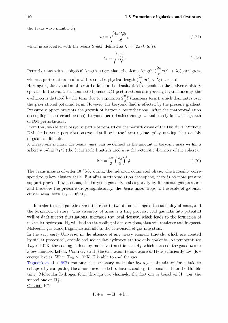
Fig. 1.2 – Relation between BH mass and the total stellar mass of local host galaxies (Reines & Volonteri,2015). This consist of a sample of 244 broad-line AGN from which the virial BH masses are estimatedthrough the single-epoch virial mass estimator (Reines, Greene & Geha, 2013) and shown as red points.Pink points represent 10 broad-line AGN and composite dwarf galaxies. Dark green point represents thedwarf galaxy RGG 118 with its 50,000 M BH. Light green point is Pox 52. Purple points represent15 reverberation-mapped AGN. Blue dots represent dynamical BH mass measurements. Turquoise dotsrepresent the S/SO galaxies with classical bulges. Orange dots the S/SO galaxies with pseudobulges.Grey lines show different BH mass- bulge mass relations.

in Kormendy & Ho (2013). For instance, galaxies NGC 1332, NGC 3091, NGC 1550, and NGC1407, have dynamical BH mass measurement of MBH > 109 M (Kormendy & Ho, 2013). Reines& Volonteri (2015) provided a sample of local galaxies hosting BHs, at z < 0.055, that wereproduce in Fig 1.2. Blue points represent BHs in quiescent galaxies, whereas red points showAGN. On Fig 1.2, we see that indeed massive galaxies can host very massive central BHs of few109 M. It is important to keep in mind that we have focussed so far on understanding what wewere able to see until today, namely powerful BHs and massive galaxies. We have only observedthe massive end of the BH and galaxy story. Understanding the BH population requires to nowmove on observing the low-mass end on the BH distribution, specifically the BHs that couldreside in low-mass galaxies. Such observations need the support of theoretical models, such asthose developed in this thesis.

Observing low-mass BHs in low-mass galaxies

That being said, observing the BH population in low-mass galaxies is not at all an easy task, formany reasons. First of all, if we simply extrapolate the BH-galaxy mass relation to low-massgalaxies, BH mass in low-mass galaxies would be lower that the ones in more massive galaxies,which makes their detections more challenging. In the hierarchical structure formation model,massive galaxies grow in mass partly because of galaxy-galaxy mergers. Low-mass galaxies,instead, do not experience as many galaxy-galaxy mergers as massive galaxies, their growth islimited compared to their massive counterparts. BH mass growth is boosted when a galaxy-galaxymerger occurs. BH in low-mass galaxies, are instead not expected to have grown much over

16 1.4 Black holes as a key component of galaxies

cosmic time.Low-mass BHs are more difficult to observe than their massive counterparts, their gravitationalforce is weaker, stars or gas moving around such low-mass BHs will be difficult to identify/observe.Stellar and gas dynamics method:Galaxies beyond the Milky Way, are too far for us to resolve individual stars trajectories aroundthe central BH. In the local Universe, we therefore need to study quantities which are averagedover stars, such as the averaged velocity of stars. In the inner part of a galaxy hosting a BH,there is an additional contribution to the gravitational potential from the BH, stars will movefaster in the presence of a BH, resulting in a higher peak in the velocity curve. However, thispeak is proportional to the mass of the BH, the more massive the BH is, faster is the velocity ofthe stars. The velocity dispersion σ along the line of sight and the surface density, and so thestellar density, can be measured and we can deduce the BH mass component. Gas dynamicsis also used in a similar way, it allows one to measure the motion of ionized gas, this methodmostly focuses on low-luminosity AGN.Accreting BH signatures:In addition to the gas moving around BHs, which provides precious clues for the detection of BHs,for example emission lines. BHs are often enclosed in an accretion disk. An accreting (potentiallylow-mass) BH can be detected via its accretion signatures. Matter that is accreted into the accre-tion disk of the BH, dissipate most of its energy in the UV wavelengths. Further BH signaturescan be identified, such as X-ray emission, resulting from the interaction of high energy particles.The emission from these BHs is also thought to be weaker too, reducing our chance to detect them.

The properties of low-mass galaxies can also complicate the detection of low-mass BHs.Low-mass galaxies contain more gas, more dust and more on-going star formation (Greene, 2012).The dust can obscure/absorb the emission (which is already suspected to be weak) from anaccreting BH. The on-going star formation emission will also make a BH detection difficult,because contaminating the diagnostics in optical, IR, and UV.Multi-wavelength search helps to select BH low-mass galaxies sample, as X-ray, radio (Galloet al., 2008, 2010 ; Reines et al., 2011 ; Reines & Deller, 2012 ; Miller et al., 2012 ; Schramm et al.,2013 ; Reines et al., 2014) and mid-infrared wavelengths (Izotov et al., 2014 ; Jarrett et al., 2011).X-ray photons from the nucleus are so energetic that they can be observed despite the gas-richcontent of the galaxy, whereas radio and mid-infrared wavelength emissions are also less impactedby dust absorption. A combination of different wavelengths is a good method to detect BHsin low-mass galaxies, we give a non-exhaustive list of new BH search using multi-wavelengthsmethod, at the end of this section. Combination of X-ray and an another wavelength can, forexample, avoid a contamination by X-ray binaries (XRBs). Indeed, the ratio of radio to hardX-ray emission is larger for accreting BHs than for stellar mass BHs (Merloni, Heinz & di Matteo,2003). Mid-IR observations allow one to detect luminous AGN (Stern et al., 2012 ; Assef et al.,2013), even if it is much more complicated to use it as an observational diagnostic to make asample of dwarf galaxies (Izotov et al., 2014 ; Jarrett et al., 2011), because of the contaminationfrom star-forming galaxies, which also emit mid-IR emission.

To conclude, low-mass BHs are complicated to observe, first because stellar or gas kinematicsmethod are less sensitive to these low-mass objects. Accreting BHs offer a better chance to beobserved. However, many sources of contamination exist, for example from the host galaxies,and make their detection difficult. New observational diagnostics emerge to detect these objects,as the combination of different wavelength search, that can avoid pollution from star-forming

Introduction 17

Fig. 1.3 – Low-mass BHs detected in galaxies, showed here in the BH mass - galaxy velocity dispersiondiagram. Not only massive galaxies harbor a BH, BHs are also found in low-mass galaxies, some galaxiesmay be bereft of BHs.

galaxies, and from XRBs, for example. In the following, we list some of low-mass BHs that havebeen detected, and we review the search for new samples of BHs in low-mass galaxies.

Examples of low-mass BHs observed in low-mass galaxies

Over the last decade we have accumulated a good deal of observational evidence of the presenceof BHs in low-mass galaxies in the local Universe. Below, we list some of the BHs that have beendetected, or not, in low-mass galaxies. We start by listing two particularly interesting cases ofnearby low-mass galaxies, which do not show any evidence for the presence of a BH, upper limitshave been assigned to these BHs. Gebhardt et al. (2001) derive an upper limit for the BH massin M33 of 1500 M through stellar kinematics, with a best fit of the light profile indicating anabsence of BH. For the same galaxy Merritt, Ferrarese & Joseph (2001) find an upper limit of3000 M. Using the same method, Valluri et al. (2005) find an upper limit of 2.2× 104 M forthe dwarf elliptical NGC 205. These very low upper limits possibly indicate that these galaxiesare lacking a BH, or at least that they contain very low-mass BHs.Low-mass BHs have been observed in several galaxies, here we list some of them in a chrono-logical order. NGC 4395 shows clear evidence for a 104 − 105 M BH (Filippenko & Ho, 2003 ;Peterson et al., 2005 ; Edri et al., 2012) (Hβ linewidth-luminosity-mass scaling relation), withrapid variability in the X-rays (Shih, Iwasawa & Fabian, 2003), and a radio-jet (Wrobel & Ho,2006). The galaxy POX 52 is thought to host a low-mass BH of ∼ 105 M as well (Barth et al.,2004). Barth et al. (2009) find that the galaxy NGC 3621 could host a 3× 106 M BH, accretionevidence is also found. The presence of a 5 × 105 M has been reported in the galaxy NGC404 by Seth et al. (2010), also with kinematics method and a set of other methods (near-IRintegrated-filed spectroscopy, optical spectroscopy, imaging, etc).Some low-mass galaxies host an accreting BH, as revealed in Reines et al. (2011) by X-ray andradio emission from the dwarf galaxy Henize 2-10, the mass of the BH is estimated at 2× 106 M.The dwarf galaxy M6-UCD1 indicates signatures of a 2.1×107 M BH. Yuan et al. (2014) identify4 candidates with BH mass of 106 M, two of which show signatures of X-ray emission.Baldassare et al. (2015) report the lowest-mass BH ever discovered, with a mass of 50,000 M,

18 1.4 Black holes as a key component of galaxies

derived through virial BH mass estimate techniques.

Search for more objects in low-mass galaxies

Despite these famous examples of low-mass BHs, in recent years, many studies have startedlooking for evidence of the presence of BHs in low-mass galaxies, in a systematic way, with stellarmass of M? ∼ 109 M. The SDSS survey is an optical spectroscopic galaxy survey (York et al.,2000). It has been used to look for evidence for accreting BHs with broad Hα line. Greene& Ho (2004) identify 19 objects (using the first release of SDSS data), which correspond tobroad-line AGN, with a BH mass in the range 8× 104 − 106 M. Mass of BHs were determinedusing a linewidth-luminosity-mass scaling relation method, which links the BH mass to the AGNluminosity at a given wavelength (at 5100 Å), and the FWHM of the broad Hβ line.Greene & Ho (2007a) estimate BH masses of AGN in low-mass galaxies though the virial method(1.27), which is a method “extrapolating” the results from reverberation mapping to single-epochspectra. The BH mass is expressed by:

MBH = fv2RBLRG

, (1.27)

where f is a scaling factor accounting for the unkown broad line region (BLR) geometry (seeGreene & Ho, 2005). The broad line region velocity dispersion is measured from the line width.The radius of the BLR region is estimated from the AGN luminosity using a radius-luminosityempirical relation derived by reverberation mapping of a sample of AGN. With the reverberationmethod, the radius RBLR of the broad-line region is determined by measuring the time delay ∆tbetween variations in the BLR emission and in the AGN photoionizing continuum. This sampleincreases by one order of magnitude the number of BHs with M < 2 × 106 M. From thissample, Dong, Greene & Ho (2012) study the X-ray properties of 49 sources in the BH mass range105−6 M, and find several weak X-ray sources. Evidence for narrow-line AGN in low stellarvelocity dispersions (favoring the presence of a low mass BH) have been found (Barth, Greene& Ho, 2008). However, because of small volume surveys, or for example SDSS spectroscopicselections which favor a selection of luminous galaxies, and the low number of galaxies withM? < 109 M, these samples did not give us all the clues needed to understand BH population inlow-mass galaxies, but have paved the way for the following low-mass BH search. Reines, Greene& Geha (2013) performed a new systematic search for BHs (of 105−6 M) in galaxies with stellarmass of M? < 3× 109 M. They found 136 dwarf galaxies harboring evidences of active BHs,in the SDSS survey. The identification is made on the detection of narrow-line photoionizationsignatures, and/or broad Hα emission lines. Lemons et al. (2015) recently identify a new sampleof BHs using hard X-ray diagnostics, meaning that this could be an interesting diagnosticsfor AGN in dwarf galaxies. More recent works use, as we have said before, X-ray and radioobservations to search for weakly accreting BHs (Reines, 2015). This allows to avoid a confusionin optical wavelengths, for example with star-forming region emission. However, recently Moranet al. (2014) show that optical detections have still a role to play in the low-mass BHs detection,by identifying 28 AGN in the SDSS survey, with BH mass estimated in the range 103 − 104 M,a sample for which only few of the objects have been also identified via emission that can be as-sociated to BH accretion in other bands than optical, for example at radio and X-ray wavelengths.

Massive BHs are found in many local galaxies, from massive galaxies, to low-mass galaxies,when other galaxies seem to be lacking of BHs. In this section, we have seen that today we

Introduction 19

are pushing the observational limits to identify more and more BHs in low-mass galaxies. Ourability of observing galaxies keeps increasing, so no doubt that many more signatures of BHs inlow-mass galaxies will emerge.

1.4.3 Population of quasars at z = 6

In the 1960s, several observational studies proposed the idea of quasi-stellar radio sources,quasi-stellar sources, that we commonly call quasars today. Observations of more and morevery luminous objects, with powerful radio emission, showing broad emission lines at uncommunwavelengths, but also variability, and excess of ultraviolet emission compared with normal stars7.Among the most famous objects, there is 3C295, which was studied by Minkowski, who showedthat 3C295 was 10 times smaller than Cyg A, and the presence of a redshifted line allowed him todeduce that the object was 10 times farther than Cyg A. In 1961, Matthews and Sandage, studied3C48, which was thought to be a small blue star, with broad emission at unkown wavelenghts.In 1962, Hazard determined the position of 3C273, and the structure of an associated elongatedradio source, similar to a jet. Schmidt and Oke observed the source and also found redshiftedlines, as in 3C48. These objects were all showing highly redshifted lines in their spectra, werevery luminous, and were also for some of them showing variability (3C48, 3C273), indicatingthat the sources were actually small. A series of papers in 1963 (Hazard, Mackey & Shimmins,1963 ; Schmidt, 1963 ; Oke, 1963 ; Greenstein, 1963), were addressing the nature of quasars, aseither unusual galactic stars, or extra galactic sources at larger redshifts. It has been quitedifficult for the community to accept that the redshifts indicated by these lines, were cosmologicalredshifts and that these sources were far away powerful extragalactic sources. Rapidly, in order toexplain the features of such quasar objects, central mass of 109 M are proposed (see Matthews& Sandage, 1963 ; Smith & Hoffleit, 1963, for example), definitely too massive to be normal stars.

Today, we observe these quasars up to redshift z = 7 (Fan et al., 2006a ; Jiang & et al.,, 2009 ;Mortlock et al., 2011), and they represent the active tail of BHs distribution. The oldest quasarever observed is ULAS J1120+0641 (Mortlock et al., 2011), which was already in place only 770Myrs after the Big Bang, at redshift z = 7.085. The mass of the BH powering this quasar isMBH ∼ 2× 109 M (estimated from the quasar luminosity and its MgII line width). Other highredshift quasars have been observed before but at lower redshift than ULAS J1120+0641, amongwhich CFHQS J0210-0456 at z = 6.44 (Willott et al., 2010a), SDSS 1148+5251 at z = 6.42 (Fanet al., 2003), and CFHQS J2329+0301 at z = 6.42 (Willott et al., 2007). A sample of 19 highredshift luminous quasars, in the redshift range 5.74 < z < 6.42, and magnitude of zAB 6 20(corresponding to a magnitude of M1450Å ∼ −27 at 1450 Å) has been described in a series ofpapers (Fan et al., 2003, 2006a). This sample has been made using the SDSS. Fainter objectshave been observed, again in the SDSS survey, with magnitude 21 < zAB < 22.16 (correspondingto magnitudes in the range −28 < M1450Å < −25). These are 6 quasars in the redshift range5.78 < z < 6, their magnitude is 2 order of magnitude fainter than the previous z ∼ 6 knownquasars found in SDSS. Their weak Lyα emission lines could be due to small black hole massesand high Eddington luminosity ratios, indicating that these BHs grow on short time scales. Someof the high-redshift quasars cited in this section are shown in Fig 1.6.

7For a very interesting review which retraces the history of the discovery of quasars, seehttps://ned.ipac.caltech.edu/level5/Sept04/Shields/Shields3.html. See also the book of Suzy Collin-Zahn, Desquasars aux trous noirs.

20 1.5 Black holes as a key component for galaxy evolution

The discovery of quasars at very high redshift, z > 6, also triggered new questions regardingthe role of powerful BHs in the early Universe, both on the evolution of galaxies, and on theevolution of the IGM. Quasars spectra allow us to answer some of these questions, particularlyconcerning the reionization of the Universe. Constraints on cosmic reionization mainly comesfrom IGM properties, how the IGM absorb and react to the radiation coming from backgroundsources. The fraction and distribution of neutral hydrogen along the line-of-sight is inferred fromquasar observations. Observing spectra of ionizing sources provide a crucial information on theproperties of the IGM (density, composition, and so on). In the most easy case, namely when theemission from the IGM is negligible, the number of photons in a line-of-sight from the source tous, can only decrease. Photons can indeed only be absorbed by the IGM, and re-emitted undera random direction, and then may be scattered away from the line-of-sight. This defines themean optical depth of the IGM, and can be probed by measuring the absorption in the spectraof quasars at high redshifts. In practice, it consists in measuring the flux decrement caused bythe IGM, which is the mean value of the ratio between the observed continuum flux (Fobs(λ))and the expected continuum flux in the absence of absorption (Fcont(λ)). This effect is known asthe Gunn-Peterson effect. Using quasars spectra, Fan et al. (2006a) show that, at z > 6, theeffective optical depth increases rapidly with increasing redshift, therefore indicating a rapidincrease in the neutral density of the IGM at z > 6 (see also, Becker et al., 2001 ; Djorgovskiet al., 2001 ; Fan et al., 2002 ; White et al., 2003). A rapid increase of HII regions size suggestingthat HI fraction of the IGM has increased by a factor of > 10 from z = 6.4 to z = 5.7 is alsoshown (Fan et al., 2006a).With the observation of the Gunn and Peterson trough effect, caused by neutral hydrogen in theIGM, in high redshift quasars, we start dating the end of the reionization period, around z ∼ 6.However, the time evolution is difficult to investigate, from this we can not know wether theIGM become neutral just after z > 6 and therefore is a rapid process, or if the reionization is aslow process occuring at redshift much higher than z = 6. The impact of accreting BHs at suchhigh redshift, whether BHs play a predominent role in the reionization process of the Universe,is still debated today.

In this section, we have seen that BHs are present both in high redshift galaxies, and in thepresent local Universe. Moreover these BHs span a large range of mass, from the smallest centralBHs observed, with MBH = 50, 000 M (Baldassare et al., 2015) to the large mass of quasars weobserve at high redshift. The most massive BH ever observed has a mass of MBH > 1010 M(McConnell et al., 2011). The mass distribution of BHs is a challenge for theoretical models ofBH formation, which must explain both the low-mass and high-mass ends of BH distribution.High redshift quasars are also challenging for BH growth models, because they are observedless than 1 Gyr after the formation of the first BHs, and therefore they must have acquiredlarge amount of mass in a short time. The detection of such massive objects at high redshift isthe first constraint that we have for BH formation and evolution, it also helped to investigatereionization, and trigger new questions regarding BH feedback. In the next section, we focus onthe co-evolution of BHs and their host galaxies, and the different mechanisms of BH feedback.

1.5 Black holes as a key component for galaxy evolution

We have seen that BHs are an important ingredient of galaxies, in the local Universe, but also athigh redshift, which is probed by the observation of quasars. The comoving density of quasarsat high redshift (z ∼ 6) is 40 times smaller than the one at z ∼ 3 (Fan et al., 2006b), this

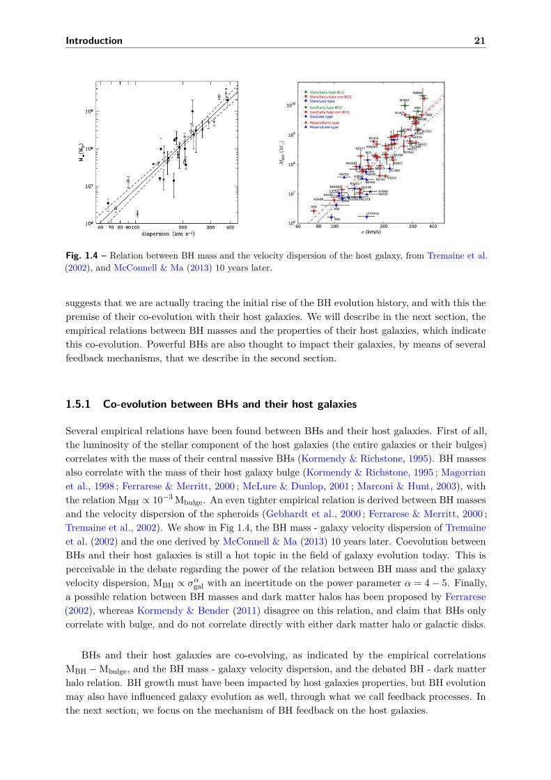
Introduction 21

Fig. 1.4 – Relation between BH mass and the velocity dispersion of the host galaxy, from Tremaine et al.(2002), and McConnell & Ma (2013) 10 years later.

suggests that we are actually tracing the initial rise of the BH evolution history, and with this thepremise of their co-evolution with their host galaxies. We will describe in the next section, theempirical relations between BH masses and the properties of their host galaxies, which indicatethis co-evolution. Powerful BHs are also thought to impact their galaxies, by means of severalfeedback mechanisms, that we describe in the second section.

1.5.1 Co-evolution between BHs and their host galaxies

Several empirical relations have been found between BHs and their host galaxies. First of all,the luminosity of the stellar component of the host galaxies (the entire galaxies or their bulges)correlates with the mass of their central massive BHs (Kormendy & Richstone, 1995). BH massesalso correlate with the mass of their host galaxy bulge (Kormendy & Richstone, 1995 ; Magorrianet al., 1998 ; Ferrarese & Merritt, 2000 ; McLure & Dunlop, 2001 ; Marconi & Hunt, 2003), withthe relation MBH ∝ 10−3 Mbulge. An even tighter empirical relation is derived between BH massesand the velocity dispersion of the spheroids (Gebhardt et al., 2000 ; Ferrarese & Merritt, 2000 ;Tremaine et al., 2002). We show in Fig 1.4, the BH mass - galaxy velocity dispersion of Tremaineet al. (2002) and the one derived by McConnell & Ma (2013) 10 years later. Coevolution betweenBHs and their host galaxies is still a hot topic in the field of galaxy evolution today. This isperceivable in the debate regarding the power of the relation between BH mass and the galaxyvelocity dispersion, MBH ∝ σαgal with an incertitude on the power parameter α = 4− 5. Finally,a possible relation between BH masses and dark matter halos has been proposed by Ferrarese(2002), whereas Kormendy & Bender (2011) disagree on this relation, and claim that BHs onlycorrelate with bulge, and do not correlate directly with either dark matter halo or galactic disks.

BHs and their host galaxies are co-evolving, as indicated by the empirical correlationsMBH −Mbulge, and the BH mass - galaxy velocity dispersion, and the debated BH - dark matterhalo relation. BH growth must have been impacted by host galaxies properties, but BH evolutionmay also have influenced galaxy evolution as well, through what we call feedback processes. Inthe next section, we focus on the mechanism of BH feedback on the host galaxies.

22 1.5 Black holes as a key component for galaxy evolution

1.5.2 AGN feedback

When gas is accreted onto a BH, there is a release of rest-mass accreted energy back to thegalactic gas, which can impact the host galaxy by feedback processes (Silk & Rees, 1998). AGNfeedback acts as an interaction between the energy, radiation produced by gas accretion onto thecentral BH, and the gas in the host galaxy. Theoretically, the energy released by the BH, can besufficient to entirely unbind the gas of its host galaxy. If BH growth is dictated by accretion, theBH energy is expressed as EBH = (ε/1− ε)MBH c2, whereas the binding energy of the galaxy isexpressed by Egal = Mgal σ

2. The ratio between the energy released by the BH and the bindingenergy of the host galaxy is:

EBHEgal

= ε

1− ε

(MBHMgal

)(c

σ

)2> 60 (1.28)

if we assume the radiative efficiency to be ε ∼ 0.1. If only a small fraction of the BH accretionenergy was released as kinetic energy transferred to the gas, AGN feedback would be able tounbind the gas of the galaxy.Three main mechanisms can alter the galaxy gas content through AGN feedback: radiationfeedback, kinetic feedback, and the ejection of energetic particles. These mechanisms have beenimplemented and tested in both isolated and cosmological simulations, leading to both negativeand positive feedback. In the following, we explain the different modes of AGN feedback, andhow they have been implemented in numerical simulations. We then explain the positive andnegative feedback effects, and review some studies which result in either one or the other aspectsof AGN feedback, and their implications.

Radiative feedback or quasar modeThe first one is radiative feedback, through both radiation pressure and radiative heating. Radia-tive pressure is the force exerted on the galaxy gas through different processes such as electronsscattering, or scattering and absorption on dust for example (see many papers by Mitch Begelman,or the corresponding review Begelman, 2004). This is what we call the quasar mode of AGNfeedback. Quasar mode is thought to happen after an episode of high gas accretion onto aBH, which can take place mostly in high redshift galaxies, which are gas-rich, and thereforeprovide a gas reservoir to feel the BH. AGN feedback through the radiative mode, is thought topush cold gas outward, when the accretion onto the central BH is close to the Eddington limit(MBH/MEdd > 0.01). Deposition of internal energy by increasing the gas temperature, has beenused in cosmological simulations to mimic the heating of the gas in the surrounding of BHs (DiMatteo et al., 2008 ; Teyssier et al., 2011 ; Dubois et al., 2012a).

Mechanical feedback or radio modeObservationally, the kinetic or mechanical feedback is the easiest to observe (through X-ray andradio observations), because responsible for the ejection of powerful jets, and bubbles/cavitiesdiscovered in the cores of clusters (see for example the Perseus cluster, Fabian et al., 2006). Innumerical simulations, this mode is modeled for low Eddington fraction (MBH/MEdd 6 0.01),with a momentum-driven kinetic bipolar outflow, where the mass, energy, and momentum aredeposited in the surroundings within a cylinder (Dubois et al., 2010, 2011, 2012a). The orientationof the outflow is determined by computing the gas angular momentum around BHs.

Ejection of energetic particlesFinally AGN feedback is also responsible for ejecting energetic particles in the surroundings,

Introduction 23

Fig. 1.5 – Cartoon from Silk & Mamon (2012), showing the theoretical galaxy mass function, and theobservational one. Discrepancies appear at both the low-mass and high-mass ends of galaxy distribution.Feedback from SN and AGN have been advocated to regulate the star formation in galaxies at low andhigh-mass end respectively.

which can be either charged (cosmic rays), or neutral (relativistic neutrons or neutrinos).

AGN feedback can be negative, the gas is heated, which inhibits star formation in the galaxy,but also dispersed and pushed out of the galaxy, which limit the gas mass available to form starsas well. Conversely, AGN feedback can impact the host galaxy in a positive way, by triggeringstar formation. Negative and positive AGN feedback are not excluding each other, and may bothexist at different times or different parts of the host galaxy (Silk, 2013).When we compare theoretical models and cosmological simulations to observations of galaxiesin the nearby Universe, we see that the models lead to an overestimate of the number of smallgalaxies, and of the number of high mass galaxies. In other words, in galaxy evolution models,galaxies and dark matter halos retain too many baryons, and produce too many stars. Thisis known as the overcooling problem. At the low-mass end of the galaxy stellar mass function,stellar feedback, by means of SN winds, are able to drive baryons out of halos. However, whenwe consider much more massive galaxies, winds from SN may not be sufficiently strong to pushbaryons out of the galaxy. Only powerful BHs are thought to be strong enough, to removebaryons or suppress accretion from the cosmic web, therefore decreasing the ability of galaxies toform stars, which leads to a decrease of the galaxy luminosity function at the high-mass end.The evolution between star formation and dark matter halo mass appears to be more complexthan what models and simulations predict, this is partially due to our lack of knowledge in starformation, and mechanism of galaxy regulation, as stellar and BH feedbacks. AGN regulating starformation in their host galaxies, what we call the quenching of galaxies, have been reproduced incosmological simulations. Di Matteo et al. (2008) and Dubois et al. (2012a), model the radiative(or quasar) AGN feedback mode, by depositing internal energy into the surrounding of BH, andfind that AGN feedback regulate star formation, and therefore have a negative feedback. Inaddition to quench star formation in massive galaxies, AGN feedback is also thought to limittheir own BH accretion by depositing energy in the surroundings (Silk & Rees, 1998 ; Fabian,1999), and to drive/regulate the coevolution between BHs and their host galaxies.

Regarding the positive impact of AGN feedback, theoretical studies (Begelman & Cioffi, 1989 ;

24 1.6 Black hole growth over cosmic time

Rees, 1989) have shown that outflow or jets propagating in an inhomogeneous ISM of galaxymay boost or even trigger star formation. This have been also demonstrated in simulations ofmassive galaxy composed by a multi-phase ISM, and including a powerful jet (Gaibler et al.,2012). The jet is able to change the shape of the density probability distribution function, andpressurize the galactic disk, which compresses gas clumps, and increases their densities up tothe limit to form stars. Positive AGN feedback has also been found in isolated galaxy hydrody-namical simulations including an ambient external pressure in the galactic disk (Bieri et al., 2016).

The radiative mode is the AGN feedback mode dedicated to high accretion rate onto the BH(close to the Eddington limit), and could therefore be the mode responsible for the co-evolutionbetween for example the BH mass and the galaxy stellar velocity dispersion, and may be thepredominant mode at early times because of the large reservoirs of cold gas available to fuelcentral BHs. Conversely, the kinetic mode responsible for driving large outflows, may be themain AGN feedback mechanism at later times, as observed today in nearby galaxies. At latertimes, gas has been consumed and pushed away by previous AGN feedback episodes, and starformation episodes, therefore the BHs accrete at a lower Eddington fraction (see also Churazovet al., 2005). We are still far from understanding the whole mechanisms of AGN feedback, andwhether it has a positive and negative effect of the host galaxies, or a contribution of the two atdifferent places, and times, and whether a given mode of AGN feedback is associated to a givenpositive or negative effect.

In the two previous sections, we have discussed the presence of massive BHs in most of thenearby massive galaxies, but also the discovery of quasars, which tells us that powerful BHswere already assembled and in their powerful age already at high redshift. We also pointedout that we have several clues on the co-evolution of these BHs with their host galaxies (fromhigh redshift to the local Universe), through empirical relations between BH mass and galaxyproperties. We have discussed the capability of BHs to interact and regulate their host galaxiesevolution, through radiative or kinetic feedback mechanisms. In the next section 1.6, we focuson BH growth.

1.6 Black hole growth over cosmic time

More than 50 high redshift quasars (z > 5, Fan, 2006) have been observed so far. They help usto constrain the high redshift Universe, and periods that are hardly accessible with observations,such as the reonization. The observation of quasars at high redshift is one of the main clueson BH formation and growth we have today. The z = 6 quasars are among the most luminousobjects that we have observed, at all redshifts. Their apparent magnitudes can be up to ∼ 19,even for redshift higher than z > 6. As we have seen, the SDSS survey strongly helped us tounderstand better the powerful quasars (Fan, 2001 ; Fan et al., 2003), and let us with a puzzelingpopulation of massive powerful BHs less than 1 Gyr after the Big Bang. The fact that we observethem at very high redshift gives us precious clues: BHs must have formed in the early Universe inorder to assemble within 1 Gyr after the Big Bang, and to grow very efficiently up to > 109 Mby z = 6 for some of them. How can BHs grow of several order of magnitude within 1 Gyr? Istheir grow limited?

Eddington limitIt exists a luminosity limit, the so-called Eddington luminosity, for which the radiation pressure

Introduction 25

is higher than the gravity, a wind is formed, and matter is pushed away from the BH. If weconsider the luminosity which can be emitted by an object via a static photosphere in a sphericalgeometry, with a small volume at the surface dV, and r the radius of the photosphere, we canexpress the gravitational force as:

dFgravdV = −GMmpn

r2 ur, (1.29)

with M the mass of the object, which is the BH here, mp the proton mass. We assume thatthe matter which is accreted is only composed of hydrogen (in neutral or ionized state). Theradiation flux interacts mainly with the matter by Thomson scattering on electrons, so the forceof radiation pressure is expressed by:

dFraddV = −nσT

c

L

4πr2 ur, (1.30)

with σT the Thomson cross-section. The resulting force is:

dF

dV = −(

1− LσT4πGMmpc

)GMmpn

r2 ur. (1.31)

We therefore define the luminosity limit, for which the radiation pressure is higher than thegravity, the photosphere is not static anymore, which leads to the formation of a wind:

LEdd = 4πGMmpc

σT= 3.4× 104

( MM

)L. (1.32)

We commonly define the Eddington timescale, or the Salpeter timescale, as:

LEdd = MBHc2

tEddwith tEdd = σTc

4πGmp= 0.45 Gyr. (1.33)

A BH accretes at a fraction fEdd of this Eddington limit:

L = εMaccc2 = fEddLEddc

2, (1.34)

with ε the efficiency with which accreted matter is converted into radiation, fEdd is the ratio ofthe luminosity and the maximum Eddington luminosity.

Macc = fEddLEddε

= fEddMBHc2

ε tEdd(1.35)

dMBH = (1− ε)dMacc (1.36)

dMBHdt = (1− ε)

εfEdd

1tEdd

MBH (1.37)

dMBHMBH

= (1− ε)ε

fEdddttEdd

. (1.38)

After integration, we obtain the time evolution of the BH mass:

MBH(t) = MBH(t = 0) exp[(1− ε)

εfEdd

tgrowthtEdd

], (1.39)

and the corresponding time of growth:

tgrowth = tEddε

(1− ε)1

fEddln[ MBH

MBH(t = 0)

]. (1.40)

26 1.6 Black hole growth over cosmic time

Fig. 1.6 – Theoretical growth of high redshift quasars. The sample of some high redshift quasars isrepresented in orange dots. Black dashed lines indicate theoretical growth of two of these objects, assumingε = 0.1, and a constant growth at either fEdd = 0.3 or fEdd = 1.

From this last equation, if we consider a quasar of 109 M as a z = 6, which had accreted at theEddington limit its entire life (tgrowth = 1 Gyr), and considering tEdd = 0.45 Gyr, we find thatthe initial mass of the BH is MBH(t = 0) ∼ 2 M. From the mass of quasars at high redshiftwe can then infer different configurations for BH formation and BH growth together. We canalready notice that accreting at the Eddington rate from the beginning of the Universe is astrong assumption, therefore BH seeds forming with masses in the range 100 − 105 M seemmore realistic. In Fig. 1.6, we show a sample of few high-redshift quasars, among which those wehave presented in the previous section, in orange dots. Black dashed lines indicate the theoreticalgrowth of the BHs powering two of these quasars, assuming ε = 0.1, and either fEdd = 0.3 orfEdd = 1. In the next section, we will describe the main theoretical scenarios that have beenadvanced for the formation of such massive BH seeds in the early Universe. Before coming tothe formation of BHs, we here briefly review different modes of BH growth.

BH growthSeveral processes participate to the growth of BHs: gas accretion, and BH-BH mergers. However,it has been shown that BH growth is mainly driven by gas accretion, rather than BH-BH mergers.This comes from both the hard X-ray background measurement (Fabian & Iwasawa, 1999) (whichgives the mass density in BHs), and Soltan’s argument (Soltan, 1982 ; Yu & Tremaine, 2002),which compares the mass of BHs today to the AGN/quasar population (through their luminosityfunctions) integrated over luminosity and redshift. This total energy can be converted into atotal accreted mass, and appears to be close to the total mass of BH today. This tends to saythat most of BH growth is done by radiatively efficient gas accretion. The luminosity L of a BHis defined by:

L = ε

1− εc2 Macc, (1.41)

and can be related to the accreted mass energy E of a BH, which is then expressed by:

E = ε

1− εc2 Macc. (1.42)

Introduction 27

The density ρacc is obtained by:

E

V= 1V

ε

1− εc2 Macc = ε

1− εc2ρacc, (1.43)

with V the volume. The luminosity function of quasars and AGN gives the number of objects Nwith the luminosity L, for the volume V :

Φ(L, t) = dN

dLdV. (1.44)

Soltan’s argument is to integrate the observed luminosity function of quasars/AGN over luminosityand time, to obtain the total energy density emitted by accreting BHs uacc:

uacc =∫ 0

tdt

∫ ∞0

Φ(L, t)LdL, (1.45)

or to integrate over redshift:

uacc =∫ ∞z

dt

dzdz

∫ ∞0

Φ(L, t)LdL. (1.46)

Finally, a comparison is established between the density of accreted mass ρacc to the total energyemitted by known accreting BHs uacc:

ρacc = uacc1c2

1− εε

= 1c2

1− εε

∫ ∞z

dt

dzdz

∫ ∞0

Φ(L, t)LdL. (1.47)

The derived local mass density of accreted matter, gives us the total amount of matter that havebeen accreted by quasars. However, it is based on the observed luminosity function of quasars,and therefore may be underestimated, because of the presence of potential obscured AGN that aremissed by observations, and the presence of normal BHs (quiescent, non-accreting BHs). Thereforethe Soltan’s argument gives a lower limit of the relic BHs that we could find in local galaxiestoday. Soltan (1982) find that the mass accumulated in quasars is ε−1 4.7× 1012 MGpc−3 =ε−1 4.7 × 103 MMpc−3, which translates into 4.7 × 1013 MGpc−3 = ε−1 4.7 × 104 MMpc−3

when we assume ε = 0.1. At that time, the quasar luminosity function was not as well-knowas today, and the local mass density found by Soltan (1982) was therefore underestimated, andalready quite large, and interestingly similar to the mass in BHs today. Yu & Tremaine (2002)derive:

ρacc(z = 0) = 2.1× 105(CB/11.8)[0.11− εε

] MMcp−3 (1.48)

This means that taking into account the total accretion onto quasars, we find that every 1 Mpc3,there must exist > 105 M mass of BH(s), which is similar to what we observe today. Thereforethe growth of BHs is mainly driven by gas accretion.

Regulation of BH growthWe have seen that BHs mostly grow by gas accretion, however, the accretion can be regulated bydifferent processes, at small scales in the close environment of the BH, and at larger scales.BH growth can be regulated in the first place immediately after the BH formation. The SNexplosion of the stellar progenitor produces two types of feedback. Feedback can be mechanical,the explosion can push the gas outward, and lead to a low-density medium around the newlyformed BH, particularly for high-redshift mini-halos with shallow potential well (Johnson &Bromm, 2007 ; Pelupessy, Di Matteo & Ciardi, 2007 ; Alvarez, Wise & Abel, 2009). It can bethermal, the SN explosion also certainly heats the gas. Finally, the star can also have produced

28 1.6 Black hole growth over cosmic time

ionizing radiation. Pop III stars are thought to produce large amount of ionizing radiation(Schaerer, 2002) before collapsing into a BH. The initial growth of the BH seed can thereforebe delayed for ∼ 100 Myr (Johnson & Bromm, 2007 ; Alvarez, Wise & Abel, 2009 ; Johnsonet al., 2013), due to the low-density region it is formed in. Conversely, BHs formed throughsupermassive stars (we will describe BH formation models in the next section), have more chanceto grow. Indeed, emitted ionizing radiation from supermassive stars could be weaker, as wellas their radiative feedback (Hosokawa et al., 2013 ; Schleicher et al., 2013), resulting in a morefavorable environment for the newly formed BH to accrete gas. Early growth of BHs depends onBH formation models, namely the BH progenitors properties, the initial mass of BH, and theclose environment they are born in. Accretion onto the BH itself can also favor the productionof ionizing radiation, decreasing the early accretion into BHs. Unfortunately, these phenomenaare difficult to capture within simulations, requiring sub-parsec resolutions.

Larger scale environment also strongly influence the growth of BHs. Cosmological simulations(Bromm & Loeb, 2003 ; Greif et al., 2008 ; Wise, Turk & Abel, 2008) have shown that an importantreservoir of gas can be produced in the inner part of proto-galaxies by the gravitational collapseof the gas. This reservoir could start or at least increase the accretion onto BHs after theirformation, counteracting the potential negative feedback from the BH stellar progenitor. At evenlarger scales, the growth of BHs is sustained by cold filamentary infall (Di Matteo et al., 2012 ;Dubois et al., 2012b). At later times, galaxy mergers can also boost the accretion onto BHs byredistributing the gas within the resulting galaxy. Several simulations have shown that when agalaxy merger occurs, gravitational tidal fields produce large inflows to galaxies center (Barnes& Hernquist, 1991, 1996, e.g. the early work), boosting the accretion onto the central BH (DiMatteo, Springel & Hernquist, 2005 ; Di Matteo et al., 2008 ; Hopkins et al., 2006).

We have seen that to explain the massive end of the BH distribution, high accretion episodesor super-Eddington accretion episodes, have been envisaged (e.g. Collin et al., 2002 ; Abramowicz,2005). Supercritical accretion onto BHs at high redshift have been studied (Volonteri, Silk &Dubus, 2015 ; Pacucci, Volonteri & Ferrara, 2015 ; Pacucci et al., 2015 ; Inayoshi, Haiman &Ostriker, 2016). The formation of accretion disks around BHs depend on the accretion rate,here m denotes the normalized accretion rate, with m = MBH/MEdd. For low accretion rates,m 6 0.01, cooling is inefficient, the disk is expanded and radiatively inefficient (Abramowicz &Lasota, 1995). For higher accretion rates, 0.01 6 m 6 1, cooling is more efficient, the accretiondisk is geometrically thin and optically thick (Shakura & Sunyaev, 1973). Finally, for muchhigher accretion rates, m >> 1, a slim accretion disk forms (Abramowicz et al., 1988). For aslim disk, the luminosity is proportional to:

L

LEdd∝ 1 + ln(m) ∝ 1 + ln( M

MEdd), (1.49)

instead of ∝ m, meaning that the disk is radiatively inefficient, and the luminosity is contained.Super-Eddington accretion does not imply super-Eddington luminosities. The phenomenonoccurring here is the trapping of the radiation. For low-angular momentum gas in the center ofgalaxies, a compact accretion disk (slim accretion disk model) can form out of the low angularmomentum infalling gas. The high compactness of the disk, implies the trapping of photons,which can not escape in a time shorter than the timescale for accretion, the luminosity remainlower than the Eddington limit. BH growth could be boosted by a factor of few times theEddington limit. Using this slim disk model, Volonteri, Silk & Dubus (2015) predict thatlong-lived super-Eddington accretion occurs only in galaxies with copious low-angular momentum

Introduction 29

gas. They are the only galaxies able to fuel central BHs at supercritical rates for sufficiently longtimes, by forming a slim disk around BHs, which is able to trap radiation for long times. Thecommonly used Eddington limit may therefore not be a real limit for BH growth.

1.7 Theoretical models for black hole formation in the early Universe

Currently, three main models are popular to explain theoretically the formation of massive BHseeds in the early Universe (Rees, 1978, 1984): the PopIII remnants model, the compact stellarcluster model, and the direct collapse model.These three models for BH formation rely on different physical processes, but the main idea isto form a massive BH out of a massive star. The mass of the star that forms out of the gas, isrelied to the Jeans mass of the medium, that we can write as:

MJ ≈ 700M(

T

200 K

)3/2 ( n

104 cm−3

)−1/2. (1.50)

The composition of the gas, and so its temperature, sets the Jeans mass. For exemple, in minihalosof Mmini halo ≈ 105−6 M, where cooling is done by molecular hydrogen, the temperature of thegas goes below 104K (see left panel of Fig 1.7). If we assume T = 200 K, the Jeans mass isMJ ≈ 700 M. We will see that massive stars of the first generation are predicted to form inminihalos.However, in atomic cooling halos of Mhalo ≈ 107−8 M, where the temperature can be T = 5000 Kfor example, the Jeans mass is much higher MJ ≈ 105 M, which can lead to the formation of aneven more massive star, which may collapse into a direct collapse BH.Finally if the gas is metal-enriched, cooling is more efficient. Indeed on Fig 1.7 right panel, wesee that the cooling curve for metal-enriched gas is above the cooling curve for a primordialcomposition of the gas. In the presence of metals, the gas can also cool to lower temperatures.Molecules made of heavy elements are responsible for lowering the temperatures to a few K.Therefore the Jeans mass will be much lower. For example, for T = 10 K, the Jeans mass isaround MJ ≈ 10 M. This is an intermediate model between the two previous ones, which iscalled stellar compact cluster model. A compact stellar cluster can form in the central region ofproto-galaxies, stars are very close to each other, and can merge together to form a very massivestar, that can collapse and form a massive BH.

1.7.1 Remnants of the first generation of stars

In the PopIII star remnants model, BHs are predicted to form in mini-halos (Mh ≈ 105 M)with gas below a critical metallicity (Z < 10−3.5 Z, Bromm et al., 2001 ; Schneider et al., 2002)at redshift z = 30 − 20 from the remnants of the first generation of stars (PopIII stars, Carr,Bond & Arnett, 1984 ; Madau & Rees, 2001 ; Volonteri, Madau & Haardt, 2003). As we havesaid in Section 1.3, observational evidence on the initial mass function (IMF) of PopIII stars arelacking, but theoretical studies suggest that they could have masses in the range 10− 1000 M(Bromm & Yoshida, 2011 ; Hirano et al., 2014). A massive star M? & 260 M can lead to theformation of a BH seed of ≈ 100 M (Fryer, Woosley & Heger, 2001), which retained at leasthalf the mass of the star.

The fate of primordial starsWe have not observed any zero-metallicity star yet. However, their existence has been studiedtheoretically. In the very early Universe, in the absence of any heavy element (metal), atomic

30 1.7 Theoretical models for black hole formation in the early Universe

Fig. 1.7 – Left panel: cooling curves for primordial composition of the gas. Right panel: cooling curvesfor primordial composition of the gas (solid line) and solar composition of the gas (dashed line).

and molecular hydrogen are the only coolants. Then, it was rather difficult for primordial cloudsto cool efficiently. Clouds and proto-stars were therefore able to grow in mass (because the Jeansmass, which is proportional to the temperature, was still high), for the gravitational force tobalance the internal energy of the gas, and collapse. As a result these stars are predicted to bemassive (Bromm & Yoshida, 2011), and to end their life within few Myrs. From Fig. 1.8, we candistinguish 4 domains for the zero-metallicity stars based on their final fate: stars with a massM? < 25 M, 25 M < M? < 140 M, 140 M < M? < 260 M, and 260 M < M?.

For the M? < 25 M regime:Stars with mass lower than 8 M form white dwarfs. Stars which are more massive than 8 Mform neutron stars.

For the 25 M < M? < 140 M regime:We can distinguish 3 different mass regimes here. First of all, for stars less massive thanM? 35 M, a BH can form by fallback. A first explosion of the star, an explosion of SN type,pushes away a significant fraction of the stellar mass by winds, which falls back and collapses toa BH keeping 10% of the initial stellar mass. For more massive stars, however, the helium coreis more massive, as well as the oxygen and silicon core masses which prevents a potential SNexplosion because of their large infall toward the center. No SNe are formed, and instead a BHforms directly. Finally the last regime consists of the stars more massive than ∼ 100 M. Forthis regime, the star experiences the electron-positron pair creation instability (that we explainin more detail in the next regime). γ photon collide with atoms of the star, and create e−/e+

pairs. The radiation pressure of the star decreases, because a part of γ photons do not contributeanymore to the pressure. Infall starts, and stops when enough energy is released, which leads toa SN explosion. For M? < 140 M stars, however, the explosion is not strong enough to totallydisrupt the star, the core can collapse and form a BH directly. The BH will keep less than halfthe initial mass of the star.

For the 140 M < M? < 260 M regime:Hydrogen forms helium by fusion. Helium in the core of the star also enters fusion reaction, that

Introduction 31

we call the central helium burning phase. When helium is fully consumed, the temperature anddensity of the star are sufficiently high for electron-positron pair creation, meaning that e−/e+

pairs are created in significant proportions. These e−/e+ pairs are the result of collisions betweenatoms present in the star and photons γ, which are abundant in massive stars. This happenswhen the energy of γ photons is higher than the energy of the created pair, for Eγ > Ee− +Ee− ,the exceeding energy of γ photons is given to the pairs. A part of the internal energy is thereforeconverted into rest mass energy through the e−/e+ pairs. However, photons that participate thereaction, do not contribute anymore to the radiation flux going outwards. Radiative pressuredecreases, and can not balance gravity anymore. The star enters an unstable phase, and contracts.The collapse increases the number of pairs annihilations, which leads to an amplification of thephoton production, which also increases the temperature of the star. Therefore more e−/e+

pairs are created, and so on. High temperature of the star, can lead to the creation of heavierelements depending of the star mass (oxygen, silicium, ...), and could stop its collapse. Under theexplosive combustion of these elements, the star ends up its life in an nuclear-powered explosion.In this regime, the energy of the explosion is higher, and can even reach ∼ 1053 erg s−1, and leaveno compact object behind, all the metals are ejected in the surrounding ISM.

For the M? > 260 M regime:For the massive end of the stellar distribution of metal-free stars, the photodisintegration processallows the star to avoid the last explosive combustion phase. Because of the high temperatureand pressure in the core, atoms can absorb very energetic photons. Atoms enter an excited state,their desexcitation is done by the emission of protons, neutrons, and α particles. The energyproduced by the combustion of elements is therefore converted, and the star can avoid the finalexplosion and disruption. Temperature and pressure are decreased by the photodisintegrationprocess, which favors the collapse, and the formation of a compact BH, able to retain at leasthalf the initial stellar mass.

Difficulties and incertainties of the PopIII remnants scenarioFirst of all, large uncertainties remain on the first generation of stars, regarding their initial mass(properties of accretion into the core, external effects may also play an important role, such asfeedback from UV radiation, CMB temperature), their number density in the early Universe,and the distribution of their formation (single stars or stellar cluster in minihalos).The incertainty on the initial mass of BHs formed through the PopIII remnants model is aproblem. Low-mass BHs will not be able to reach the center of the galaxy’s potential well, theywill instead interact dynamically with other objects as BHs and stars, and wander into their hostgalaxy, which does not favor high accretion rate into BHs. They would hardly accrete enoughmass to form the population of quasars we observe at z = 6 (e.g. Pelupessy, Di Matteo & Ciardi,2007).This is even worse if we consider that they produce large ionizing radiation, which can heat thesurrounding gas, and leave a potential BH in a low density environment, not very propitiousfor high accretion episodes of the seed. Simulations with radiative transfer coupled to thehydrodynamics (Alvarez, Wise & Abel, 2009), modeling the radiation form the PopIII starprogenitor, have allowed one to study BH growth immediately after the death of the PopIIIprogenitor. BH growth is regulated by radiative feedback, which alters the accretion flow fromlarge scales (see also, Milosavljevic et al., 2009), and keeps the BH in a low-density and hightemperature gas environment, resulting in a low accretion rate into the BH. Therefore, radiativefeedback makes even more difficult the growth of BH (Alvarez, Wise & Abel, 2009).

32 1.7 Theoretical models for black hole formation in the early Universe

Fig. 1.8 – The fate of primordial stars (zero metallicity, non-rotating), from Heger et al. (2003). The figureshows the initial mass of primordial stars (x-axis), the stellar mass at time of final explosion/remnantformation (thick blue line), and the mass of the remnant object that is left behind after the death of thestar (y-axis, thick red line). Metals released are shown in green filled and hatched regions. Four mainscases are distinguished based on their final fate: the fate of stars M? < 25 M leads to the formation ofwhite dwarfs and neutron stars, stars within the range 25 M < M? < 140 M will form a BH, stars withinthe range 140 M < M? < 260 M will leave no compact remnant behind, and finally stars 260 M < M?

will lead to the formation of massive BHs.

Introduction 33

However mechanisms for super-Eddington accretion have been developed (Volonteri, Silk &Dubus, 2015 ; Madau, Haardt & Dotti, 2014 ; Lupi et al., 2016). Episodes of super-Eddingtonaccretion could allow PopIII remnant BHs to reach mass consistent with high redshift quasars.Lupi et al. (2016) simulate a idealized cluster of stellar mass BHs orbiting the inner part (∼ 200 pc)of a gas-rich galaxy. They model BH thermal feedback, which allows for different periods ofradiatively inefficient accretion burst, during which the BHs can accrete mass at super-Eddingtonaccretion rate. They find that the growth of the simulated BHs, acquiring ∼ 103−4 M on Myrtimescales, is consistent with the the mass that should have quasars progenitors.

1.7.2 Compact stellar clusters

The death of the first generation of stars, inevitably leads to the release of metals into thesurroundings, galactic winds can then push these metals farther, and pollute nearby halos. In thepresence of metals, cooling is more efficient, ensuring fragmentation in these nearby halos. Theformation of a second generation of stars is therefore initiated (Omukai, Schneider & Haiman,2008), these PopII stars are less massive than the PopIII stars. Indeed, gas cooling is moreefficient due to the presence of metals and molecules, and therefore the Jeans mass is smaller,the gas fragments and leads to the formation of less massive PopII stars.Compact nuclear clusters often inhabit the center of galaxies. Such a cluster in the inner part ofgalaxies at high redshift, in relatively metal-poor environments, could have collapsed and form avery massive star, up to ∼ 1000 M, by stellar collisions.At high redshift, dense regions in proto-galactic disks, distributed uniformly in the entire disk,would fragment into several clumps, when their mass reaches the Jeans mass, and therefore wouldlead to star formation in the entire disk. In Toomre-unstable disks, instead, instabilities can leadto mass inflow toward the disk center, no fragmentation happens. Therefore the density of thecentral part of the disk increases, and star formation only occurs at the center of the galaxy. Acompact stellar cluster forms in the central region. For metallicity of 10−4 − 10−5 Z, the typicalmass of the cluster is 105 M, the half mass radii is ∼ 1pc (Devecchi & Volonteri, 2009 ; Regan& Haehnelt, 2009a ; Volonteri, 2010).The stars and the parent cluster evolve on more or less the same timescales, the evolution ofstars and the cluster dynamics are coupled, and therefore difficult to study. Portegies Zwart et al.(1999) use N-body simulation to study the evolution of young compact stellar clusters. A clusterof different mass stars is more likely, in this case massive stars will segregate from the others lessmassive ones, because of dynamical friction, then increasing the probability for these stars tocollide. Runaway collisions between stars can happen, leading to the formation of a very massivestar, which can collapse into a BH.Metallicity appears to be a crucial parameter in this scenario, for two main reasons. First ofall, because in metal-poor environment stars are more massive, and stars > 40 M are predictedto collapse directly into a BH without exploding in SN (Heger et al., 2003). The second reasonis that runaway collisions between stars lead to a significant mass loss (Portegies Zwart et al.,1999).However, for metal-poor stars, mass loss is reduced. The metal-poor conditions are thereforerelated to mass losses through winds. Yungelson et al. (2008) study the stellar evolution ofsolar composition stars in the mass range 60− 1000 M. They find that they shed most of theirmass via winds and are expected to end their lives as BHs less massive than ∼ 150 M. At lowmetallicity, instead, mass loss due to winds is much more reduced, thus increasing the mass ofthe final remnant (Heger et al., 2003 ; Vink, 2008 ; Mapelli, Colpi & Zampieri, 2009 ; Belczynski

34 1.7 Theoretical models for black hole formation in the early Universe

et al., 2010 ; Mapelli et al., 2013 ; Spera, Mapelli & Bressan, 2015).A metal-poor environment therefore favors the formation of a more massive star at the beginning,but also its growth. A BH seed of 103 M can be formed in this nuclear cluster model (?Devecchi& Volonteri, 2009 ; Regan & Haehnelt, 2009b ; Katz, Sijacki & Haehnelt, 2015). Devecchi &Volonteri (2009) find that 5% of protogalaxies at z = 20−10, could form a BH by this mechanism.

1.7.3 Direct collapse of gas

One recent way of solving the problem of the formation of such massive objects is by the directcollapse of pristine gas triggered by dynamical processes (Loeb & Rasio, 1994 ; Eisenstein &Loeb, 1995 ; Koushiappas, Bullock & Dekel, 2004 ; Begelman, Volonteri & Rees, 2006 ; Lodato &Natarajan, 2006 ; Mayer et al., 2010), or invoking isothermal collapse in primordial halos (Bromm& Loeb, 2003 ; Spaans & Silk, 2006 ; Dijkstra et al., 2008 ; Latif et al., 2013a) . This scenario hasbecome very popular, as it can lead to the formation of 104 − 106 M seeds, making it easier toreproduce the quasar population at z > 6. All these models rely on different physical processesand have so different requirements, among which avoiding the fragmentation of the gas, angularmomentum transport, metal-poor environment, large inflow rate of gas. We first describe modelswhich can be classified as dynamical processes, and then move to isothermal collapse models.

Direct collapse model requires to avoid the fragmentation of the gas, and also the accumulationof mass in halo center, to form only one massive object in the center. Several models based ondynamical processes have been studied.Turbulent systems (with supersonic turbulence), metal-free or not, have been shown to suppressthe fragmentation of the gas (Begelman & Shlosman, 2009). The non-requirement of metal-freeor metal-poor conditions of halos, makes this model feasible at lower redshift and in metal-richhalos. The formation of BHs in metal-rich galaxies has also been investigating more recently(Mayer et al., 2010, 2014). In this model, a stable compact nuclear disk forms, and is fulfilledwith large accretion rate of ∼ 104 M, as a result of metal-rich galaxy merger. The disk canthen collapse and form a BH. We will see later than the fragmentation of the gas can also beprevented in the presence of LW radiation, that suppress H2.Angular momentum transport is crucial to form a massive object in halo center, mass needs totravel inwards, and the angular momentum outwards. Indeed, to form a unique and massiveobject, mass needs to accumulate at the center of the halo. Gravitational systems, such ashalos, are thought to possess a given degree of rotational support, which is described by the spinparameter λspin = J |E|1/2/GM5/2

h , with J the angular momentum of halos, E the total energy,and Mh the mass of halos. The angular momentum of a halo, or its baryonic central region, isthought to be the result of clustering/surrounding neighbors applying tidal torques on the givenhalo (Peebles, 1969). Before collapsing into a single massive object, the gas needs to settle into arotationally supported proto-galactic disk (for example, see Oh & Haiman, 2002). BH formationin low angular momentum environment is supported by analytical models. Eisenstein & Loeb(1995) used an analytical model to investigate the origin of BHs from the collapse of low-spincosmological perturbations. They derived the spin distribution of halos, and found that enoughlow-spin halos to explain the population of BHs. Koushiappas, Bullock & Dekel (2004) studiedinstead the formation of BHs in low angular momentum gas, present in all halos massive enoughto host an unstable self-gravitating disk. They only consider the low angular momentum tail ofmaterial of halos. A fraction of low-spin gas should lead to an infall of gas in the central region,and to its collapse. Transport of angular momentum to lead to large infall of mass through the

Introduction 35

center of the disk is generally still needed.Dynamical instabilities, either global (Shlosman, Frank & Begelman, 1989 ; Begelman, Volonteri& Rees, 2006) or local (Lodato & Natarajan, 2006), are among the processes to transport angularmomentum. Bars within bars model is one of the angular momentum transport mechanisms(Begelman, Volonteri & Rees, 2006). Halo gas cools and collapses gradually until rotationalsupport halts the collapse. When rotational support becomes important, self-gravitating gasclouds can become bar-unstable. Therefore, gravitational and hydrodynamical instabilities leadto angular momentum transport along the bar. Because the gas is able to cool, the systemcontracts, more instabilities are therefore created within the system, a new bar is formed, and soon. The transport of the angular momentum outwards allows the mass to travel inwards. Themechanism forms a supermassive star, its core can collapse into a BH of 10− 20 M. Accretionforms the envelope can lead to high accretion rate into the BH, located in the core. The BHgrowth is limited by the Eddington limit of the whole system (BH in the core and the wholequasi-star), and therefore high accretion into the BH are possible while the BH mass is lowerthan the mass of the envelope (Begelman, Volonteri & Rees, 2006).Redistribution of angular momentum and mass, can also be achieved via local instabilities(Lodato & Natarajan, 2006), for marginally stable disks in protogalaxies (stability of the diskis determined via the Toomre parameter), when the disk gets massive enough to be stable.When the Toomre parameter of the disk is close to the limit for stability, the disk experiencesgravitational instabilities, that can lead to mass infall to the center of the disk, instead of gasfragmentation. Once enough mass has been transported to make the disk stable again, theprocess stops, and a massive star-like object can form in the center.

The physical conditions (listed below) required for isothermal collapse in primordial halos,which has become the most popular version of direct collapse in the last couple of years, andwhose BH seeds are typically referred to as “DCBHs”, are numerous. First, one needs a halo thathas reached the atomic cooling threshold, ∼ 107 − 108 M, but it is still pristine, i.e., metal-free(metal-free or metal-poor were not required for most of the scenarios listed in the previoussection). A large inflow rate of gas at the center of the halo is also required. Angular momentumtransport has also an important role, as discussed in the previous section. In the following, wedevelop in more detail these conditions for the isothermal collapse model.One needs that the molecular hydrogen formation has been suppressed throughout the halo’sevolution. The presence of metals and molecular hydrogen would decrease the temperature ofthe gas, and so the Jeans mass. This could lead to the fragmentation of the gas cloud, thereforethe formation of only one massive object is unlikely, and the formation of several less massiveobjects, namely PopIII stars, is instead expected.The destruction of molecular hydrogen can be accomplished by strong photo-dissociating radiation(Lyman-Werner, LW, photons with energy between 11.2 eV and 13.6 eV), and its prevention byphoto-detachment of H−. The destruction of H2 is characterized by the reaction:

H2 + γLW −→ H + H (1.51)

In this channel, which is based on the Solomon process, photons in the energy range 11.2−13.6 eVcan be absorbed by H2 (in the LW band), H2 accedes an excited state, and photodissociates themolecule. For the photo-detachment of H−, we have the following reaction:

H− + γ0.76 eV −→ H + e− (1.52)

The rate of H− decreases, this prevents the formation of H2 via the H− channel.Trapping of Lyman α photons could increase the temperature of the gas, therefore destroying

36 1.7 Theoretical models for black hole formation in the early Universe

H2, it would also stiffen the equation of state, and make more difficult the fragmentation of thegas (Spaans & Silk, 2006).

Radiation intensity Jcrit:Jcrit (in units of 10−21 erg s−1 cm−2 Hz−1 sr−1) defines the level of LW radiation intensity re-quired to dissociate a critical fraction of H2, and depends on the stellar population, namely theblack-body curves, and the ratio of 0.76 eV photons to LW photons produced by these stellarpopulations (Shang, Bryan & Haiman, 2010 ; Wolcott-Green, Haiman & Bryan, 2011).Omukai (2001) use a 1D-zone model where spherical clouds are irradiated by photodissociatingradiation, and find that when Jcrit ∼ 105, both suppression of H2 formation, and photodissocia-tion of H2, prevent H2 cooling. Bromm & Loeb (2003) use 3D hydrodynamical simulations andshow that for a thermal spectrum with T?,III = 105 K, Jcrit > 105, and for a lower temperatureT?,II = 104 K, Jcrit > 103, which is consistent with the previous 1D analysis of Omukai (2001).Temperature T?,III = 105 K refers to a Pop III population, whereas T?,II = 104 K refers to aPopII population. Shang, Bryan & Haiman (2010) using 3D hydrodynamical simulations of halosand a 1D model similar to Omukai (2001), find lower values (by a factor up to 10) for the criticalradiation intensity, which can be due to a more accurate rate of H2 collisional dissociation.From this model, it is commonly admitted that a PopIII stellar population (T?,III ∼ 105 K) leadsto Jcrit = 103 − 104, whereas a PopII population (T?,II ∼ 104 K) to Jcrit = 30 − 100 (Shang,Bryan & Haiman, 2010).

The difference in the critical radiation intensity for PopIII and PopII stars is also due tothe abundance of 0.76 eV photons with respect to the LW photons. H− is photodetached viareaction 1.52. More 0.76 eV photons are produced for PopII stars than PopIII stars, compared toLW photons (Omukai, Schneider & Haiman, 2008), offering another channel for the destructionof H2 molecules. Therefore, the contribution of LW photons, which is encoded in the criticalradiation intensity Jcrit, does not need to be as high for PopII stars as for PopIII stars.A single value for the critical radiation intensity is unlikely, instead a spread on a distributionof possible values is expected, as discussed by Sugimura, Omukai & Inoue (2014) ; Agarwal &Khochfar (2015) ; Agarwal et al. (2015b).In any case, the value derived by the models cited above (i.e. Jcrit = 30 − 100), are muchlower than the radiation intensity that is required in 3D cosmological hydrodynamical zoom-insimulations. A radiation intensity of Jcrit > 500− 1000 is found in Regan, Johansson & Wise(2014) ; Latif et al. (2014, 2015).The star-forming galaxies that can provide photo-dissociating LW radiation, are susceptible toalso provide X-ray radiation, which can travel in the inner part of halos, and ionize the gas. Thisleads to an enhancement of the formation of H2. Inayoshi & Tanaka (2015) show that takinginto account X-ray ionization can indeed increase the critical flux to even higher values, andtherefore decreasing the number density of BHs (see also Latif et al., 2015).

PopIII vs PopIIThe LW radiation intensity is expected to be mainly driven by PopII stars, for different reasons.First, a small radiation background will impact stellar formation, H2 is photo dissociated, whichdecreases the cooling and the formation of PopIII star (Agarwal et al., 2012 ; Johnson et al.,2012). Agarwal et al. (2012) use a semi-analytical model of radiation intensity variation ontop of a DM simulation. They compute the star formation rate of PopIII stars, which dropsat z = 16, when PopII stars start forming. Johnson, Dalla Vecchia & Khochfar (2013) run

Introduction 37

cosmological simulations with and without LW radiation. Here again PopIII star formation dropsat z ∼ 11− 12. PopIII star formation rate appears to be regulated by LW feedback.Second, the life time of PopIII stars is shorter than the PopII star, their contribution to providea high radiation intensity is certainly limited. The lifetime of a PopIII star is ∼ 10 Myr. Sinceone halo must be illuminated by the LW radiation for at least one free-fall time to collapse andform a DCBH, one can compute the redshift at which the free-fall time is approximately equalto ∼ 10 Myr, which is z ∼ 45. If a DCBH forms in a halo illuminated only by Pop III stars, itshould form at very early time around z ∼ 45.Another argument is that the radiation flux produced by Pop III stars only, does not provideenough radiation intensity to provide the critical intensity Jcrit commonly assumed for DCscenario (Agarwal et al., 2012). Finally, the abundance of PopII stars is higher than the PopIIIone, and therefore they are also expected to contribute more to the radiation intensity for thisreason.

A large inflow rate of gasA large inflow rate of gas at the center of the halo, higher than 0.1 M/yr, and sustained for atleast 10 Myr, is also needed to form a supermassive star-like object in the nucleus (Begelman,Volonteri & Rees, 2006 ; Begelman, Rossi & Armitage, 2008 ; Begelman, 2010 ; Ball et al., 2011 ;Hosokawa, Omukai & Yorke, 2012 ; Hosokawa et al., 2013 ; Schleicher et al., 2013). An additionalargument for the few Myr time scale for the accretion time scale is the life time for massive stars.Basically all the mass must accrete before the main-sequence life time is up. In the absence ofH2, the collapse proceeds isothermally at the temperature of ∼ 8000 K, the accretion onto thecentral region is driven by warm gas flows, with an accretion rate of order the free-fall rate:

m ∼ c3s

G ∼ 0.1(

T

8000K

)3/2M/yr (1.53)

with cs the sound speed, T the temperature of the gas. The BH mass can be up to 90% of thestellar mass.

Number density of DCBHBecause of all the strict conditions that we have enumerated, namely the absence of efficientcoolants as molecular hydrogen or metals, and therefore the destruction of H2 by a strongphoto-dissociating flux, but also a high accretion rate into the halo center, the DCBH scenario ispredicted to be quite rare. The scenario predicts the formation of very massive seeds of about∼ 105 M, which are the perfect candidates for the population of quasars we see up to z = 6− 7.Over the last decade, the question of the number density of BH formed through the DC scenariohas therefore been studied, and via different methods: semi-analytic models, or recently hybridmodels where the spatial distribution of halos is taken from cosmological simulations. Among thesemi-analytical models, Dijkstra et al. (2008) derive a number density of 10−6 − 10−8 cMpc−3.Dijkstra, Ferrara & Mesinger (2014) investigate several physical processes, among which metal-polluted galactic winds, and derive the number density of DCBHs for different Jcrit. In Fig. 1.9,we show the number density derived by Dijkstra, Ferrara & Mesinger (2014), for various models.Few studies have taken advantage of the spatial information that cosmological simulationsoffer (Agarwal et al., 2012 ; Habouzit et al., 2016b, for dark matter only simulations), speciallyhydrodynamical ones when one can track metal-enrichment (Agarwal et al., 2014 ; Habouzit et al.,2016a). Agarwal et al. (2012) find a higher number density than the previous pure semi-analyticalmodels, around 10−1 cMpc−3 for Jcrit = 30, for the same critical intensity Agarwal et al. (2014)

38 1.8 Diagnostics to distinguish between BH formation scenarios

Fig. 1.9 – Number density of DCBHs from Dijkstra, Ferrara & Mesinger (2014). Triangles representtheir fiducial model, with Jcrit = 300, star formation occurring in all dark matter halos with Tvir > 104 K,escape fraction fesc = 1, including metal-pollution from galactic winds. Green stars represent the samemodel without taking into account pollution by galactic winds. Black circles represent the fiducial model,but decreasing the critical radiation intensity to Jcrit = 100, and for red circles to Jcrit = 30. Blue squaresrepresent the fiducial model, decreasing the escape fraction to fesc = 0.2.

find a number density of the same order.We do not develop further the number density of DCBH in this section, neither the large spreadof values that have been derived by the various models cited above. We will assess these questionsin detail in chapter 3.

1.7.4 Other models

Other BH formation models have been studied, such as primordial BHs. Those are predicted toform before the epoch of galaxy formation in regions where high density fluctuations are large,the whole region is predicted to collapse to form a BH. These primordial BHs would have massof order the particle horizon mass at their formation time (Carr, 2003):

MPBH(t) ∼ c3t

G∼ 1015

(t

10−23s

)g. (1.54)

Therefore if primordial BHs form at the Planck time (t = 10−43 s), there initial mass would beequal to the Planck mass (MPBH = 10−5 g). If BHs form at 1 s, there mass would be much higher(MPBH = 105 M).

1.8 Diagnostics to distinguish between BH formation scenarios

BHs form in the early Universe, out of any possible observation with current facilities. Investigat-ing the formation of BHs, therefore requires to derive observational diagnostics on the galaxieswe can observe today, the local galaxies, in analogy with galactic archeology. Two theoreticaldiagnostics to distinguish between the different BH formation models, have been discussed in theliterature (Volonteri, Lodato & Natarajan, 2008 ; Volonteri & Natarajan, 2009 ; van Wassenhove

Introduction 39

et al., 2010).The BHs we observe today, have grown over cosmic time from lower-mass BH seeds. Initialconditions are likely to be erased if accretion onto BHs is efficient. BHs grow by accretion andBH-BH mergers. Accretion onto a BH is boosted when galaxy-galaxy major mergers occur.Massive galaxies have a high probability that their central BH is not pristine anymore. Thecentral BH may indeed have increased its mass through accretion, which is boosted by severalmajor mergers of the host galaxy, but also BH-BH mergers and dynamical interactions. Clues onthe BH initial mass are erased. However, low-mass galaxies, which have a much quieter cosmicevolution, host a BH today with a mass that is expected to only differ slightly from the initialBH seed mass. Therefore the mass of BHs in today’s low-mass galaxies can provide us crucialinformation on the initial BH mass distribution.

Accretion and mergers alter the initial mass of BHs. The presence of a BH or not within agalaxy is, however, not affected. The probability for a galaxy to host a BH, the BH occupationfraction, is therefore a sensitive clue on the efficiency of BH formation mechanisms at highredshift. Moreover, signatures in low-mass galaxies are even stronger (Volonteri, Lodato &Natarajan, 2008). This can help us to distinguish between BH formation models, as illustratedin Fig. 1.10 reproduced from Greene (2012). On the top, the two most popular scenarios to formBHs are reproduced. On the left, the direct collapse scenario is predicted to form BHs only infew massive halos, because of the many conditions required by the scenario. On the right, we seethat many galaxies will host a PopIII remnants BH: conditions to form these BHs are less strict.Using semi-analytical models, associated with the extended Press-Schechter formalism, Volonteri,Lodato & Natarajan (2008) study comparisons of the BH mass - galaxy velocity relation fordifferent seeding models, and show that the fraction of galaxies without BH increases withdecreasing halo mass at z = 0. Moreover, while PopIII remnants scenario leads to populatenearly all z = 0 galaxies, the direct collapse scenario has a much smaller efficiency to establishBH in galaxies. van Wassenhove et al. (2010) use similar techniques to simulate specificallythe evolution of BHs in satellite galaxies of a Milky Way size halo, and study the properties ofBHs in satellites surviving until today. They seed the high redshift progenitor halos with BHseeds, formed through the PopIII remnants and direct collapse models. They find that the directcollapse BH population is present in only a few percent of dwarf galaxies, but that they aremore massive, and could be detected more easily. Whereas the PopIII remnant BHs are moreabundant in low-mass galaxies, but they are predicted to be difficult to observe because of theirvery low masses.Finally, the idea of a plume emerges in Volonteri & Natarajan (2009). Stellar remnant-likescenarios predict the formation of light seeds (MBH,ini ∼ 100 M), the direct collapse scenario,instead, predicts the formation of heavy seeds (MBH,ini ∼ 104−6 M). As discussed earlier, crucialclues on BH formation can remain in low-mass present-day galaxies, BHs there are predictedto not have grown much over cosmic time. Therefore, if the direct collapse model was thepredominant model of BH formation, we should detect in low-mass galaxies a threshold forthe minimal mass of BHs, which would correspond to an asymptote, or a plume, in the BHmass - galaxy velocity dispersion diagram, when moving to lower galaxy velocity dispersions.Investigating this plume requires to have the resolution to detect large samples of low-massgalaxies, and to go to lower and lower galaxy mass, what we are starting to do (Reines, Greene& Geha, 2013).

In practice, many difficulties appear when trying to determine the BH mass distribution in

40 1.8 Diagnostics to distinguish between BH formation scenarios

Fig. 1.10 – BH occupation fraction is one of the diagnostics to distinguish between BH formation scenarios.In the cartoon (Greene, 2012), on the top, the two most popular scenarios to form BHs are reproduced.On the left, the direct collapse scenario is predicted to form only in few massive halos, because of themany strict conditions required by the scenario. On the right, we see that many galaxies will host a PopIIIremnants BH, conditions are less strict. The Universe evolve, halos and galaxies merge. The bottompictures show two realizations of today’s Universe. On the left, only 50% of the galaxies Mgal < 109 Mhost a direct collapse BH, on the right, instead, up to 90% Mgal < 109 M galaxies host a BH.

Introduction 41

low-mass galaxies, and the occupation fraction (Greene, 2012 ; Reines, Greene & Geha, 2013).Difficulties to detect BHs in low-mass galaxies have already been discussed in section 1.4.1., weonly recall, here, the main ideas. Observationally, we are always biased by luminous objects,observing faint objects is of course more challenging. Samples are often made with opticaldiagnostics, which are only sensible to powerful accreting BHs. We are missing BHs which areaccreting at low accretion rate. Low-mass BHs are quite faint, even if they are accreting at theEddington limit. Small galaxies are not the easiest galaxies to observe either, they are oftenshowing signatures of on-going star formation, therefore one has to distinguish between emissionlines due to the presence of a BH and of the star formation episode. The presence of gas and dustin abundance is also problematic because absorbing or masking the accretion properties of BHs. Insection 1.4.1., we have highlighted recent works, that provide alternative observational diagnosticsto detect galaxies hosting a central BH, and that will be used in the future to make larger samples.

Measuring the occupation fraction is even more challenging. Recently, Miller et al. (2015)investigate the occupation fraction of Mgal < 1010 M within the AMUSE survey (X-ray detec-tion) of early-type galaxies. They find a lower limit of > 20% for the occupation fraction ofthese galaxies. On Fig. 1.11, we show the occupation fraction derived by Miller et al. (2015).This thesis aims to provide a theoretical framework of BH formation models, and to derivetheoretically several properties as the distribution of BH mass, and the occupation fraction inlow-mass galaxies, that can be compare to the future observational data.

Finally, several works have recently look beyond the local Universe to investigate the pop-ulation of BHs in low-mass galaxies Mezcua et al. (2016) realize an X-ray stacking analysisof dwarf galaxies with M? 6 3 × 109 M in the COSMOS field for z < 1.5. An X-ray excess,which is an evidence for accreting BHs, is found in each bin from z = 0 to z = 1.5, used forthe stacking method. BH masses are estimated to ∼ 105 M. This show that BHs in low-massgalaxies exist in that redshift range, however stacking analysis does not allow an estimation ofthe BH occupation fraction. Pardo et al. (2016) perform a search for BHs in dwarf galaxiesM? 6 109 M beyond the local Universe, up to z 6 1, to quantify the AGN fraction in galaxies.This approach gives an upper limit on the occupation fraction of BHs in dwarf galaxies. Thisstudy use X-ray data, and also multi-wavelength method is used to derive galaxies properties.BH masses are estimated using the empirical relation between BH mass and stellar mass, whichlead to masses in the range MBH ∼ 105 − 106 M. They find an AGN fraction of 0.6-3% forgalaxies in the range 109 M 6 M? 6 3× 109 M, and 0.1 6 z 6 0.6, which is in agreement withwhat is found in the local Universe (Reines, Greene & Geha, 2013 ; Miller et al., 2015). Thisis also in agreement with semi-analytical models which study jointly BH and galaxy formationand evolution (Somerville et al., 2008 ; Hirschmann et al., 2012a), and allow one to predict theBH occupation fraction or the AGN fraction, for example. Our work, specifically chapter 3 is acomplementary approach to the one used in semi-analytical models (see Hirschmann et al., 2012a,for a comparisons between hydrodynamical simulations, and semi-analytical models, in terms ofgalaxy content evolution), physical processes (metal enrichment, stellar and BH feedback, etc)evolve self-consistently within cosmological hydrodynamical simulations, and also allow one topredict the BH occupation.

42 1.8 Diagnostics to distinguish between BH formation scenarios

Fig. 1.11 – BH occupation fraction is one of the diagnostics to distinguish between BH formation scenarios.Miller et al. (2015) investigate the occupation fraction of Mgal < 1010 M within the AMUSE survey(X-ray detection) of early-type galaxies. They find an lower limit of > 20% for the occupation fraction ofthese galaxies.

Introduction 43

1.9 Organization of the thesis

The thesis is organized as follows. The present chapter gave an introduction of the physics andprocesses needed for the evolution of large-scale structures, the formation of the first stars andgalaxies, and gives an introduction of the observational discovery of quasars and active galacticnuclei. We have described the main features of supermassive black holes, which are thought topower the powerful objects cited above, including their growth and their formation through themain popular mechanisms that have been derived theoretically.

Chapter 2 gives an overview of the main numerical tools used in this thesis. We describe thenumerical code Ramses, which has an hydrodynamical solver, with adaptive mesh refinement.We also briefly mention the other simulation code Gadget used in this thesis.

In chapter 3, we describe our implementation of BH formation models in the cosmologicalhydrodynamical code Ramses, accounting for the PopIII stellar remnants and stellar clustertheoretical scenarios (light seed models). In this chapter, we investigate BH formation, andthe distribution and early growth of BH seeds. We also perform a comparison of three differ-ent SN feedback implementations in order to understand the impact of SNe on the formationand growth of BHs. We compare the simulated BHs to observations of Lyman-Break Analogsand BHs of a local sample. We also describe the next step of this analysis, which is to under-stand what triggers the mass accretion onto BHs, to do so we follow in time BHs in the simulations.

Chapter 4 focuses on another BH formation scenario (heavy seed model), the direct collapsemechanism, which can lead to the formation of 105 M BHs at early time of the Universe. Weperform cosmological hydrodynamical simulations of different sizes and resolutions, with thecode Ramses. This allows us to investigate the impact of different physical processes, such as SNfeedback, or critical radiation intensity, for example. We also directly investigate the question ofDCBHs as the precursors of the quasars we observe at z = 6, with the large scale simulation,Horizon-noAGN. It consists of the largest simulation box used to study the DC scenario so far,and gives a first global view of the scenario. We derive the number density of DCBHs for allthe simulations used in this work. We perform a comparison between different previous studies,including pure semi-analytical and hybrid models, and investigate the discrepancies between them.

In chapter 5, we investigate the consequences of primordial non-Gaussian perturbations ongalaxy formation/evolution, reionization, and finally on black hole formation/evolution. Weuse the code Gadget-2, and run several dark matter simulations with either Gaussian ornon-Gaussian conditions with several models of the non-Gaussian parameter fNL. Various semi-analytical models are used to paint galaxies, and black holes on dark matter halos.

Chapter 6 concludes on all the studies made in this thesis.

44 1.9 Organization of the thesis

Chapter 2Numerical simulations

To capture the non-linear evolution of the Universe, numerical simulations are an essential tool.They are designed to study both the formation and evolution of large scale structures, such asfilaments, dark matter halos, clusters of galaxies, and physical processes happening at galacticscales, such as galaxy formation and evolution, stellar formation, stellar feedback, but alsofeedback from black holes. This requires several orders of magnitude in spatial and gas densityscales. A fine resolution is needed for dense gas regions, such as halos and galaxies, but is notrelevant for large void regions. Cosmological hydrodynamics codes use two main methods toresolve this scale problem: the adaptive mesh refinement (AMR, or Eulerian codes) and smoothparticle hydrodynamics (SPH, or Lagrangian codes). The main codes using the AMR techniquesare ART (Kravtsov, Klypin & Khokhlov, 1997), Flash (Fryxell et al., 2000), Ramses (Teyssier,2002), and Enzo (O’Shea et al., 2004). The main codes using the SPH method, are Gasoline(Wadsley, Stadel & Quinn, 2004), Changa (Menon et al., 2015), and Gadget (Springel, Yoshida& White, 2001). Codes, like Arepo (Springel, 2010), which takes the main advantages of boththe Eulerian and Lagrangian approaches, have been developed.In this thesis, we have mainly used the code Ramses. Ramses is a tree-based AMR hydrodynam-ical scheme coupled with a N -body solver. In the following, we describe in detail the principle ofthe AMR code Ramses, in term of adaptive mesh refinement, N-body solver, hydrodynamicalsolver, gas cooling/heating, and the sub-grid physics regarding star formation, SN feedback andblack holes. A second part is dedicated to the SPH Gadget, that we have employed for the lastchapter of the thesis.

45

46 2.1 Ramses: a numerical code with adaptive mesh refinement

Contents2.1 Ramses: a numerical code with adaptive mesh refinement . . . . . . 46

2.1.1 Adaptive mesh refinement . . . . . . . . . . . . . . . . . . . . . . . . . . 462.1.2 Initial conditions . . . . . . . . . . . . . . . . . . . . . . . . . . . . . . . 472.1.3 Adaptive time-stepping . . . . . . . . . . . . . . . . . . . . . . . . . . . 472.1.4 N -body solver . . . . . . . . . . . . . . . . . . . . . . . . . . . . . . . . 482.1.5 Hydrodynamical solver . . . . . . . . . . . . . . . . . . . . . . . . . . . . 51

2.2 Sub-grid physics to study galaxy formation and evolution . . . . . . 522.2.1 Radiative cooling and photoheating by UV background . . . . . . . . . 522.2.2 Star formation . . . . . . . . . . . . . . . . . . . . . . . . . . . . . . . . 532.2.3 Equation-of-state . . . . . . . . . . . . . . . . . . . . . . . . . . . . . . . 542.2.4 SN feedback and metal enrichment . . . . . . . . . . . . . . . . . . . . . 542.2.5 BH formation . . . . . . . . . . . . . . . . . . . . . . . . . . . . . . . . . 562.2.6 BH accretion . . . . . . . . . . . . . . . . . . . . . . . . . . . . . . . . . 562.2.7 AGN feedback . . . . . . . . . . . . . . . . . . . . . . . . . . . . . . . . 57

2.3 Smoothed particle hydrodynamics code Gadget . . . . . . . . . . . . 57

2.1 Ramses: a numerical code with adaptive mesh refinement

2.1.1 Adaptive mesh refinement

In the adaptive mesh refinement (AMR) method, grid cells describe the values of density ρ,velocity v, and energy e. The method is Eulerian, meaning that the cells are static, and thegas can flow between them. Higher resolution is achieved in dense regions where the cell sizesare adaptively refined. Conversely, regions with low density are not refined and have a coarserresolution. Dark matter and stars are considered as collisionless particles that only interactgravitationallyThe first AMR method, developed in Berger & Oliger (1984), uses an Eulerian hydrodynamicsscheme where a hierarchy of nested grids, namely rectangular grid blocks (called patches) ofvarious sizes and resolutions, covers high-resolution regions of the flow. This is the patch-basedAMR method, the main advantage is that there is no need for domain decomposition, eachprocessor can handle a level or a patch. There is no need to have parent or child cells on thesame CPU. However, the lack of real domain decomposition can also be a negative aspect, whendoing post-processing analysis, because one CPU does not correspond to a physical region inthe simulation box. Contrary to this patch-based AMR method used in the codes ENZO andFLASH, the codes ART (Kravtsov, Klypin & Khokhlov, 1997) and Ramses (Teyssier, 2002)use a tree-based AMR method. The tree-based AMR method can be applied to any system,while patches follow clustering. There is a real domain decomposition, therefore a given region isattributed to a given CPU, which makes the post-processing analysis simpler and faster. Thedata structure is simple, and uses oct-tree, that we represent on Fig. 2.1. In a tree data structure,parent cells can be refined into children cells on a cell-by-cell basis. An oct-tree is a smallgroup of 2Ndim cells, and has 8 associated pointers: 1 parent cell, 6 neighboring parent cells,8 children octs, and 2 linked list indices. There are then two different types of cells: leaf cellshave no children cells and are considered as active, and split cells are refined and considered as

Numerical simulation 47

Fig. 2.1 – Oct tree structure, with the main oct (at level 2), pointing at both the parent oct (at level 1),and the children oct (at level 3).

inactive cells. The base of the tree is composed of cells which are all at the same level levelmin ofrefinement, which is called coarse level. The coarse gird is a regular cartesian grid. The drawbackof tree-based AMR methods is that data managing is much more complex than in patched-basedAMR methods.A smoothing criterion is applied using the free parameter nexpand to refine neighboring cells of arefined cell, in order to avoid large discontinuities in the mesh structure. The refinement can beset up using different criteria, such as particle mass, gas density, and all users can implementtheir own refinement conditions. We choose to use a mass criterion, if a cell contains more than8 times the initial mass resolution of the coarse grid, this cell is refined into children cells.The domain decomposition uses the space-filling curve Peano-Hilbert, this creates a list containingall the cells of the simulation.

2.1.2 Initial conditions

Numerical simulations firstly rely on building initial conditions. A Gaussian (or non-Gaussian, asdeveloped in chapter 5) perturbation field is generated according to a given power spectrum. Theinitial conditions generated assign initial velocities to all particles on the grid. The simulation codethen evolve these particles through cosmic time, according to an N -body and a hydrodynamicalsolvers that we describe in the following sections.

2.1.3 Adaptive time-stepping

Time-stepping is said adaptive, which means that sub-levels can have their own time-step, butthe global time-step must be the same than the sum of all the sub time-steps, in order to keep aglobal evolution of the simulation box at every global time-step. There are 4 conditions that thetime-step needs to fulfill, we list them below.

• The time-step ∆t must be shorter than the free-fall tff time ∆t < min(tff), where tff =√3π/32Gρ, with G the gravitational constant, and ρ the density of the cell.

• A particle, moving at the velocity vpart, can not travel more than a fraction of the cell size

48 2.1 Ramses: a numerical code with adaptive mesh refinement

∆x within one time-step, ∆t < ∆xmax(vpart)

.

• Sound waves can not propagate more than one cell size within one time-step (CourantFriedrich Levy CFL condition, Courant, Friedrichs & Lewy, 1967),

∆t < ∆xmax(vx + cs, vy + cs, vz + cs)

, with (vx, vy, vz) the particle velocity components.

• For cosmological simulations, a last condition is added, that the variation of the expansionfactor can not exceed 10% within one time-step, ∆t < aexp

aexp, with aexp the expansion factor,

and its time derivative aexp.

2.1.4 N-body solver

Dark matter (DM) is one the main ingredients in our Universe, and interacts only through gravity.DM is therefore referred to as collisionless matter interacting via gravity. The evolution of theDM fluid is described by two equations, which are the Vlasov and Poisson equations. Solvinggravitational dynamics requires to solve this set of two equations. In cosmological simulations,ideally one would like to model DM with billions of billions of collisionless particles, and to followeach of them individually. Unfortunately this remains impossible with our computational powertoday. Therefore DM is modeled as a distribution function f(x, p, t) of collisionless particles,particles are described at any time by their position x and velocity v or momentum p. Thisconsists of an approximation of the real evolution of DM, which is more and more exact whenthe number of DM particles used in the simulation is increased. Vlasov’s equation (also know asthe collisionless Boltzman equation) is:

dfdt = ∂

∂tf(x, p, t) + x∂

∂xf(x, p, t)−mOxΦ(x) ∂∂pf(x, p, t) = 0. (2.1)

The Poisson equation is written as:

∆Φx = 4πGm∫f(x, p, t)d3p. (2.2)

To solve this system of equations, one can use two methods, the first one is a pure N-bodyapproach, and the second one a particle-mesh (PM) method. The pure N-body approach treatsthe problem with the entire ensemble of particles. The Poisson integral becomes the directsummation of all the interaction forces between each pair of particles. The problem scales asN2, with N the number of DM particles. For the PM method, the real space is discretized on a3D grid (instead of 6D if one discretizes the entire phase-space problem), and it uses particleswith real velocities. This method allows one to not compute every particle-particle forces as inthe pure N -body method. This speeds up significantly force computation because particles donot interact anymore by pairs, but instead interact with the density field projected on the grid.The problem now scales as N × log(N). However, this still leads us with a very large numberof particles to deal with, the mass is therefore distributed in particles, which are not physicalself-gravitating particles, one numerical “macro" particle accounts for a ensemble of physicalparticles with a total mass m.

To solve the system of Vlasov and Poisson’s equations, main steps are:

• Computing the mass density ρ on the mesh (the grid) using a Cloud-In-Cell (CIC, Hockney& Eastwood, 1981) interpolation scheme. We show in Fig. 2.2 the principle of the CIC

Numerical simulation 49

Fig. 2.2 – Principe of the Cloud-In-Cell interpolation scheme. The particle is associated to its correspondingcell, which is the cell overlapping the most with the particle cloud. Particle mass is distributed to theneighboring cells, proportionally to the particle cloud area overlapping them.

interpolation scheme. Indeed, the first thing the code needs to calculate is the potential Φ,which only depends on the density ρ (Poisson’s equation). The easiest approach to computethe mass density would be to assign the mass of a particle to the single cell it belongs to,but this would create large fluctuations. Instead, the particle mass is split between thecells around the particle.

• Solving the potential Φ(x) on the mesh using the Poisson equation. Different types ofPoisson solvers can be used, for example the relaxation methods (i.e. the Jacobi or Gauss-Seidel methods), which are based on iterative procedures. These methods do not needto do massive operations over the whole volume, and do not need the exact solution ofPoisson’s equation (all solvers can only provide an approximation to the real solution inany case), but only an approximation sufficient at the accuracy level.To solve Poisson’s equation ∆Φ = 4πGρ, we can replace second order partial derivatives withsecond order finite difference approximations, which can be written as Φi+1− 2Φi + Φi−1 =4πGρidx2 (in 1D), with i the grid index. Therefore one has to solve an equation of thetype AΦ = ρ, with A a square symmetric matrix as:

−2 1 0 01 . . 00 . . 10 0 1 −2

Φ1.

.

Φn

∝ρ1.

.

ρn

(2.3)

Ramses uses the conjugate gradient method, which is an iterative method that solvessystems of linear equations. Here Φ is the unkown vector, the matrix A and the vector ρare known. A is symmetrical, so it exists a basis of normal eigenvectors of A. Knowing allthe eigenvectors of A leads to the solution Φ, however, when A is a large matrix, solving theproblem is complicated. Instead, an iterative procedure can provide us with a sufficientlygood approximation of the solution.A function f can be defined as f(Φ) = 1

2ΦTAΦ− ρTΦ, the vector Φ minimizes the functionf(Φ). The function f(Φ) is minimized by setting its gradient f ′(Φ) (also called residual)equal to 0. With A symmetric, it writes:

f ′(Φ) = AΦ− ρ. (2.4)

Indeed, if one sets the gradient to 0, with f ′(Φ) = AΦ− ρ = 0, one gets the equation tosolve, namely AΦ = ρ. The goal is to get closer to f ′(Φ) = 0 in the phase space in 2D. It

50 2.1 Ramses: a numerical code with adaptive mesh refinement

start with an initial estimate (an initial “guess” of the solution) of the vector Φ, and eachiteration will drive us closer to the solution, namely f ′(Φ) will decrease with every iteration.The initial estimate of the solution is therefore improved by iteratively decreasing theresidual f ′(Φ). The search direction could be orthogonal to the previous vector direction,and then it takes the minimum along this direction, and then another iteration would lead tothe search in the orthogonal direction of the previous search direction. Instead, to do feweriterations, the code searches the minimum along the direction which is A-orthogonal. Thedirection along which we look for the minimum is therefore orthogonal to all the previousdirections where the code already has done the minimisation. The old search vectors arekept in memory and used to construct the new direction of search vector, therefore feweriterations are needed, which is the advantage of this method. The code stops iteratingwhen

∣∣∣Φn+1 − Φn∣∣∣ < accuracy, n denotes the iteration index. Some additional iterations

can be done in order to verify that the minimum has been found.

• Computing the acceleration on the mesh (meaning for each cell) using a standard finite-difference approximation of the gradient. This allow us to know the gradient of thepotential.

• Computing each particle acceleration required to interpolate back the acceleration to theparticles using an inverse CIC interpolation scheme, through the relation:

dvidt = −OΦ, (2.5)

with i the index of particle.

• Updating each particle velocity according to its acceleration, and each particle positionaccording to its velocity.The explicit Euler time integrator can be written as:

(x, v)n+1 = (x, v)n + dt f((x, v)n), (2.6)

with f = (mv,−dΦdx). This allows us to update the position and velocity of a particlefrom the time-step n to the next time-step n+ 1. The difficulty arises from the fact thatvelocity and force are changing during the time-step. The most common time integrator isthe drift-kick-drift, which is defined by:

#»xn+ 12 = #»xn + ∆t

2#»v n. (2.7)

The velocity is then computed using the force (which correspond to the acceleration −OΦ)at mid-point, and the position is updated with the new velocity:

#»v n+1 = #»v n + ∆t#»

F

m( #»xn+ 1

2 ) (2.8)

#»xn+1 = #»xn+ 12 + ∆t

2#»v n+1. (2.9)

In this section, we have seen how DM collisionless dynamics is modeled within the N -body solver.The next section is dedicated to the hydrodynamical solver of simulations.

Numerical simulation 51

2.1.5 Hydrodynamical solver

The evolution of the hydrodynamical system is governed by Euler’s equations, expressed as thethree following equations: equation of continuity for the mass, momentum equation and energyequation:

∂ρ

∂t+∇.(ρv) = 0 (2.10)

∂

∂t(ρv) +∇.(ρv ⊗ v) +∇p = −ρ∇Φ (2.11)

∂

∂t(ρe) +∇.[ρv(e+ p

ρ)] = −ρv.∇Φ, (2.12)

with ρ the mass density, v the fluid velocity, e the specific total energy, p the thermal pressure.One needs to add a closure equation to identify a unique solution for this system of equations.This is done by the equation-of-state (EOS) of the gas:

p = (γ − 1)ρ(e− 12v

2), (2.13)

where γ = CpCv

is the gas adiabatic index, with for instance γ = 5/3 for a monoatomic gas. Theenergy equation is conservative if we remove the source terms on the right-hand side of theprevious equations (for example, here the gravitational term).

We define the vector V i as a numerical approximation to the cell average value of (ρ, ρv, ρe)at time tn, and for cell i. Therefore, the Euler system of equations, can be written as:

∂V

∂t+ O.F (V ) = 0 (2.14)

with F = (ρv, ρv ⊗ v, ρv (e+ p/ρ)) the flux. With this discretization, the equations become:

V n+1i − V n

i

∆t +Fn+1/2i+1/2 − F

n+1/2i−1/2

∆x = Sn+1/2i , (2.15)

where Fn+1/21+1/2 is the time centered flux across cell interfaces, and V n

i the average value of V inone cell at time tn. The gravitational source term is expressed as:

Sn+1/2i = (0, ρ

ni ∇Φn

i + ρn+1i ∇Φn+1

i

2 ,(ρv)ni ∇Φn

i + (ρv)n+1i ∇Φn+1

i

2 ). (2.16)

In other words, mass, momentum and energy change in time as a function of incoming fluxand/or leaving flux. To determine these fluxes at the interfaces of cells, one needs to solvethe Riemann discontinuity at each cell boundary, imposing S = 0 (operator splitting). Theinterpolation method used in Ramses is a second-order Godunov method, which corresponds tothe piecewise-linear interpolation method (PLM) introduced by Van Leer (1979). Other methodshave been introduced, such as the piecewise constant method (PCM), or the piecewise parabolicmethod (PPM). These methods reconstruct the behavior of the system taking into account notonly the mean value at the cell boundary, but also the values of the neighboring cells. Boundaryconditions are therefore needed, 2 ghost zones are needed in each direction and sides for thePLM method, one oct-tree has 2Ndim cells in Ramses, therefore 3Ndim − 1 neighboring octs areneeded to constitute the boundary conditions. In total the PLM scheme uses 6Ndim cells. ThePLM interpolation method introduces some dispersions and oscillations around discontinuities,

52 2.2 Sub-grid physics to study galaxy formation and evolution

to limit this effect, the slope in the interpolation can be limited. It avoids the formation of newextrema in the flux values, suppressing oscillations. Therefore we use a Harten-Lax-Van LeerContact Riemann solver (HLLC), with a Min-Mod total variation diminishing scheme to linearlyinterpolate the cell-centered values to their edge locations. The HLLC solver only considers thetwo fastest waves out of the three generated waves, which are the rarefaction wave moving to thedensest medium, the shock wave moving to the less dense region, and the intermediate contactwave also moving to the less dense region. This is an approximation to the exact resolution ofthe Riemann problem, the advantages is the fastest calculation of the (approximate) solution.

2.2 Sub-grid physics to study galaxy formation and evolution

To study galaxy formation and evolution, one needs to take into account baryonic processes,which mostly have a role at galaxy scales, beyond what can actually be resolved in cosmologicalsimulations. Sub-grid physics have been developed over the years to account for these un-resolvedprocesses in large scale simulations. In the following, we describe the current sub-grid physicswhich is implemented in Ramses, and shared by most of the cosmological codes (through differentnumerical implementations). Our simulations include sub-grid physics for gas cooling, heating,star formation and feedback, BH formation, accretion, and feedback from active galactic nuclei.

2.2.1 Radiative cooling and photoheating by UV background

The temperature of the gas depends on the net cooling function Λnet, which can be expressedas the sum of a cooling therm Λ, and a heating term H due to photoionization of the gas fromyoung stars:

Λnet = H+ Λ. (2.17)

Radiative cooling is modeled with the cooling curves of Sutherland & Dopita (1993), the gascools through H, He, and metals (Courty & Alimi, 2004). We show on Fig. 1.7 the cooling rateof primordial environments and environment with metals.

Several radiation cooling processes are considered for gas of primordial composition: collisionalexcitation between atoms which emit photons when reverting to their ground state, collisionalionization between atoms which lose energy by emitting an electron, electronic recombinationwith photon emission, bremsstrahlung or free-free (radiation is produced by the deceleration of acharged particle (electron) when deflected by another charged particle, and emitting a photon,the particles are both free, which means that they do not belong to an atom for example), andCompton ionization.Primordial gas can cool down to T = 104 K, mainly driven by collisional reactions in the ISM.Temperatures of the warm ISM are typically around T = 104 − 106 K. The gas around galaxiesis hotter, the cooling is there driven by free-free radiation cooling. Star formation takes place inthe regions of galaxies at low temperature and high density. To cool below T = 104 K the gasneeds the contribution from metals and molecules. A contribution from metals is included to thecooling function in Ramses.The metallicity of the gas is modeled as a passive variable (pOv = 0), which makes it easilytrackable over the gas flow through cosmic evolution. An initial zero metallicity is assumedfor most of the simulations describes in this thesis, but some use a metallicity background ofZ = 10−3 Z. The cooling curve of gas with metals has roughly the same slope of the H2 coolingcurve, therefore we use an initial background in metallicity to mimic H2 cooling. This consists of

Numerical simulation 53

an approximation, and does not exactly reproduce the H2 cooling curve, and the fact that H2formation rate is, for example, dependent of the gas density.Physical processes, such as SN explosions and star formation, modify and redistribute themetallicity over neighboring cells.To mimic reionization, photoheating from an uniform ultraviolet radiation background is added(following Haardt & Madau (1996)), taking place after z = 8.5 for most of the simulations thatwe have run.

2.2.2 Star formation

Star formation takes place in sub-parsec regions, in cold molecular gas clouds, which are denseand at low temperatures. Star formation appears as the gas gravitational collapses with atimescale defined by the free-fall time:

tff =√

3π32Gρ. (2.18)

Observationally, the Kennicutt law (1998) links the star formation rate (SFR) per unit area withthe gas surface density. This law can be transformed to give the volume density of stars as afunction of the volume gas density. In Ramses each cell follows the Schmidt law (Rasera &Teyssier, 2006):

dρ?dt

= ρ

t?(ρ) if ρ > ρ0, (2.19)

dρ?dt

= 0 if ρ < ρ0, (2.20)

with ρ0 a free parameter corresponding to the star formation threshold, this parameter isresolution-dependent, and set by the user. The star formation timescale depends on the localoverdensity of the gas via the relation:

t? = t0

(ρ

ρ0

)−1/2, (2.21)

with t0 the star formation characteristic time, which can be seen as the efficiency for the gas tocollapse and form stars:

t0 = tff(ρ0)ε

, (2.22)

withε = tff(ρ)

t?(ρ) . (2.23)

The star formation is entirely described by the timescale t0 and the density threshold ρ0. Atevery timestep ∆t, in each leaf cell with a density exceeding the user-defined threshold ρ0, anumber of star particles N are created, following a Poissonian random process. The probabilityto form N star particles is:

P (N) = λ

N ! exp−λ, (2.24)

withλ =

(ρ∆x3

m?

)∆tt?, (2.25)

with ∆x the side length of a cell, and m? the stellar resolution of the simulation. In star formingcells, all star particles are grouped to form a unique particle, with a mass Nm?. To avoid emptygas cells, only 90 % percent of the gas density can be used to from stars within a single cell.

54 2.2 Sub-grid physics to study galaxy formation and evolution

Fig. 2.3 – We use a polytropic equation of state to increase the gas pressure in cells with a high density(ρ > ρ0), to limit excessive gas fragmentation. It mimics the heating of the interstellar medium from stars,and processes that take place at small scales that we do not resolve here.

2.2.3 Equation-of-state

Gas follows an adiabatic equation-of-state (EoS) for monoatomic gas with adiabatic index γ = 5/3,except at high gas densities ρ > ρ0, where we use a polytropic EoS to increase the gas pressurein dense gas in order to limit excessive gas fragmentation by mimicking heating of the interstellarmedium from stars (Springel & Hernquist, 2003):

T = T0

(ρ

ρ0

)κ−1, (2.26)

with T the gas temperature, T0 the temperature threshold, ρ0 the density threshold, and κ thepolytropic index of the gas. We use κ = 1.6 for the polytropic index, and T0 depends on thesimulation resolution.For our set of simulations Chunky, which are used in chapter 4, where the spatial resolution is∼ 80 pc, and the dark matter resolution is 1.6× 107 M, we have used a temperature thresholdof T0 = 103 K, and a density threshold ρ0 = 1 H cm−3. For Tiny, which has a spatial resolutionof ∼ 7.6 pc, and a DM resolution of 2082 M, we have used T0 = 102 K, and ρ0 = 30 H cm−3. Inchapter 3, we have used three simulations SuperChunky, which have the same spatial resolutionand a DM resolution of 1.65 × 106 M, we have used the same parameters as the simulationChunky, namely T0 = 103 K, and ρ0 = 1 H cm−3.

2.2.4 SN feedback and metal enrichment

A large contribution of the interstellar medium metal enrichment is due to SNe. Massive starsexplode into SNe when they die, producing blast waves expanding to larger spatial scales. Incosmological simulations, SN explosions are modeled as sub-grid physics. In this thesis we haveused and compared three different SN feedback implementations: a simple thermal SN feedback,a kinetic SN feedback, and a delayed cooling SN feedback.Current numerical simulations, particularly cosmological simulations, do not resolve star individ-ually. Instead, we use star particles that represent an ensemble of stars. SN feedback is then notdone for individual stars, but for a mass fraction of each star particle. Therefore it is crucialto use an IMF, to compute the mass fraction of the star particles that will end up in SNe. We

Numerical simulation 55

model type II SNe assuming a Chabrier initial mass function (Chabrier, 2003), where ηSN = 20%of the mass fraction of stars end up their life in type II SNe, and release eSN = 1050 erg M−1

,and return metals with a yield of 0.1. We describe, here, the main characteristics of the threedifferent SN feedback models implemented in Ramses.

Thermal SN feedback

We use the thermal SN feedback implemented in Ramses, which is a weak feedback comparedto the following ones (as we will see in chapters 3 and 4). The mass ejecta mSN is computedas a fraction of the star particle: mSN = ηSN ×mstar particle, with ηSN the mass fraction of starswhich end up in type II SNe. The corresponding mass loss is removed from the mass of thestar particle. Metals are also distributed into the surrounding cells. Internal specific SN energyEthermal is released in the neighboring cells, it can be expressed by:

Ethermal = mSN × eSN = ηSN ×mstar particle × eSN. (2.27)

The energy liberated during an SN explosion is resolution-dependent, via mstar particle.

Kinetic SN feedback

The kinetic SN feedback (Dubois & Teyssier, 2008) is modeled to reproduce a Sedov blast wave,where energy, mass and momentum are deposited in the neighborhood. Sedov blast wave is theresult of a large energy deposition within a small volume. For each exploding star particle, ejectaare carried out and entrained into the surrounding gas by the blast wave. The maximum radiusof the ejecta is set equal to two cells, rmax = 2∆x. Hydrodynamical quantities of cells withinrmax are updated to account for the Sedov blast wave.

Delayed cooling SN feedback

The third model is called delayed cooling (Teyssier et al., 2013), which we modify in the sameway as Dubois et al. (2015) (i.e., parameters are resolution-dependent). After a SN explosion,the coupling of the energy to the gas is not trivial to model, because the energy released bythe explosion can be stored by non-thermal processes, such as unresolved turbulence, magneticfields, cosmic rays, which are not modeled in hydro-dynamical simulations. These processes willdissipate their energy on potentially longer timescales, defined as the dissipative time tdiss. Inorder to mimic the energetic and pressure enhancement by the non-thermal component, gascooling is prevented in gas cells where the non-thermal energy component (or non-thermal velocitydispersion σNT) is larger than some user-defined threshold (Stinson et al., 2006 ; Teyssier et al.,2013). We adopt the implementation of Dubois et al. (2015) in order to match the values of tdissand σNT to that required for the blast wave to propagate over a Jeans length (4 high-resolutioncells), the parameters are therefore resolution-dependent. We explode only one stellar particleout of 10 stellar particles, with 10 times more SN specific energy to add up stochasticity. Theevolution of the non-thermal energy can be written as:

σ2NT = 2ηNT

1051erg10M

tdisstff(ρ)ε? (2.28)

σNT =(

2ηNT1051erg10M

Ncell∆x)1/3 (32Gρ0

3π

)1/6(2.29)

56 2.2 Sub-grid physics to study galaxy formation and evolution

tdiss =(

2ηNT1051erg10M

ε?

)−1/3

(Ncell∆x)2/3(32Gρ0

3π

)−1/6. (2.30)

The implementation of SN feedback in numerical simulations has important consequences onmetal-enrichment. We can evaluate the radius of the shock Rshock (spherical in an homogeneousmedium), which is defined by the Sedov blast wave solution:

Rshock = ξ

(eSN × t2

ρ

)1/5

, (2.31)

with ξ a dimensionless parameter of order unity, ρ the density of the medium, eSN the energy ofthe SN, and t a given time.

This gives us a characteristic length of metal pollution in the medium. We will see that thedifferent implementations of SN directly impact star formation, meta-enrichment, and thereforealso BH formation. Indeed, BH form in metal-free environments, therefore the compactnessof metal-enriched bubbles allow for more metal-free regions where gravitational collapse maylead to the formation of compact objects, such as BHs. This will be discussed in more detail inchapters 3 and 4.

2.2.5 BH formation

Cosmological simulations have mostly focussed on studying the growth of BHs and AGN feedback,rather than their formation. In order to reproduce succesfuly the AGN luminosity function,various state-of-the-art simulations (e.g. Sijacki, Springel & Haehnelt, 2009 ; Di Matteo et al.,2012 ; Hirschmann et al., 2012b ; Dubois, Volonteri & Silk, 2014 ; Sijacki et al., 2015 ; Volonteriet al., 2016) have seeded halos above a fixed mass threshold (typically M 1010 M) with∼ 104 − 105 M BHs. Our implementation of BH formation, is different to these models, and isrepresented in the next chapter in detail. We use sink particles to model the formation of BHs,they are able to accrete gas from surroundings, and to merge together.

2.2.6 BH accretion

The accretion on the BH is described by the minimum between a Bondi-Hoyle-Lyttleton accretionrate and the Eddington accretion rate, with:

MBH = 4παG2M2BHρ

(cs2 + v2)3/2 ,

where α is a density dependent boost factor (Booth & Schaye, 2009), G is the gravitationalconstant, MBH the mass of the BH, ρ the average density of the medium, cs the average of thesound speed, and v the average velocity of the gas relative to the BH. The boost factor α isequal to (ρ/ρ0)2 when ρ > ρ0 and 1 otherwise.When a BH forms, namely when its corresponding sink particle is created, it is actually distributedon an ensemble of cloud particles (∼ 2000 cloud particles), equally distributed in space around thesink particle. These cloud particles are important to compute the spatially averaged quantitiesthat we describe below. The quantities ρ, and cs, are averaged around the sink particles usingthe cloud particles. Each cloud particle reads up the value of density, sound speed and velocityfrom its position in the grid of the simulation, by using the CIC method. A “Bondi-Hoyle radius”value (noted rBo−Ho in the following) is first computed, this value only depends on the propertiesof the cell where the sink particle, representing the BH, sits. This Bondi-Hoyle radius is used to

Numerical simulation 57

weight the contribution of each cloud particle in the computation of the quantities ρ, and cs. Thecell in which each cloud particle is sitting is, therefore, assigned a weight of w ∝ exp(−r2/r2

k), ris the distance between the cloud particle and the sink particle, and is defined by:

rk =

∆x4 if rBo−Ho <

∆x4

rBo−Ho if ∆x4 6 rBo−Ho 6 2∆x

2∆x if rBo−Ho > 2∆x

(2.32)

with rBo−Ho the Bondi-Hoyle radius, defined by rBo−Ho = GMBH/c2s , with cs measured at the

location of the sink particle.The accretion is limited by the Eddington accretion rate:

MEdd = 4πGMBHmpεrσTc

,

where mp the proton mass, εr = 0.1 the radiative efficiency, and σT the Thomson cross-section.

2.2.7 AGN feedback

In this thesis, AGN feedback is modeled with an isotropic injection of thermal energy into thesurrounding gas, within a sphere of 4 cells (4×∆x) around sink particles (Teyssier et al., 2011 ;Dubois et al., 2012b). We store the rest-mass energy of the accreted mass into the BH, andrelease it when the energy is high enough to raise the temperature of the gas around the BHto at least 107 K (the model is inspired by Booth & Schaye, 2009). The energy is releasedas thermal energy, with an efficiency of εf = 0.15 (calibrated to reproduce the observationalMBH −M? and MBH − σ? relations, following Dubois et al., 2012a), within a spherical bubbleof 4 cells (4 × ∆x) centered around the sink particle. Two situations can be distinguished. Ifthe gas environment of the BH is dense and cold, reaching the temperature threshold is moredifficult, the energy is accumulated and at some point a burst of energy is released, and impactsthe surroundings. In the other hand, if the gas surrounding the BH is hot and less dense, thethreshold for AGN feedback is reached faster, and the AGN is more continuously releasing energyinto the surroundings.

As said in section 1.5.2, more recent AGN feedback models have been implemented, forexample with two modes depending on the accretion rate into the BH. The radio mode ormechanical AGN feedback is effective for ˙MBH/ ˙MEdd 6 0.01, and is modeled with a kineticbipolar outflow/jet, where the mass, energy, and momentum are deposited in the surroundingwithin a cylinder (Dubois et al., 2010, 2011, 2012a). Whereas for the quasar mode or radiativeAGN feedback, which is effective for accretion rate onto the BH close to the Eddington limit( ˙MBH/ ˙MEdd > 0.01), internal energy is deposited into the surroundings to increase the gastemperature, and mimic the heating of the gas (Di Matteo et al., 2008 ; Teyssier et al., 2011 ;Dubois et al., 2012a).

2.3 Smoothed particle hydrodynamics code Gadget

Contrary to AMR codes like Ramses, smoothed particle hydrodynamics code (SPH) codes use aLagrangian approach. The fluid (namely, DM, star and gas) is discretized into particles, andbecause Lagrangian, dense regions of the simulation box are naturally refined, and acquire ahigher resolution (i.e. it decreases the length between particles). Gas properties are derived via

58 2.3 Smoothed particle hydrodynamics code Gadget

smoothing of the surrounding particles, anywhere in the simulation box.In this thesis, we only have used DM only simulations, run with the code Gadget-2, andexplained in chapter 5, therefore in the following we only describe briefly the N -body solver, butnot the hydrodynamical solver that can be used, neither the sub-grid physics which is used inthe hydrodynamical version of the code.Gadget uses a tree algorithm (or hierarchical multipole expansion) to compute gravitationalforces on short-range scales, which is coupled to a particle-mesh PM scheme for long-rangegravitational forces. This combination of two methods is called a TreePM hydrid method. AN -body solver is used, similar to the one describe in section 2.1.4. Phase-space density issampled with N particles. Particles are grouped in cells and oct-tree, their gravity is thereforeconsidered as a single multipole force. As in Ramses, cells are divided into split cells up toleaf cells. The gravitational force is computed from the base of the tree to upper levels. In theoptional TreePM method, the potential can be split into long and short-range components, asΦ = Φshort + Φlong. The long-range component is computed with mesh-based Fourier methods,whereas the short-range component is computed in real space.

Chapter 3Pop III remnants and stellar cluster models

Massive BHs inhabit local galaxies, including the Milky Way and some dwarf galaxies. BHformation, occurring at early cosmic times, must account for the properties of BHs in today’sgalaxies, notably why some galaxies host a BH, and others do not. We investigate the formation,distribution and growth of BH ‘seeds’ by using the adaptive mesh refinement code Ramses. Wedevelop an implementation of BH formation in dense, low-metallicity environments, as advocatedby models invoking the collapse of the first generation of stars, or of dense nuclear star clusters.The seed masses are computed one-by-one on-the-fly, based on the star formation rate and thestellar initial mass function. This self-consistent method to seed BHs allows us to study thedistribution of BHs in a cosmological context and their evolution over cosmic time. We findthat all high-mass galaxies tend to a host a BH, whereas low-mass counterparts have a lowerprobability of hosting a BH. After the end of the epoch of BH formation, this probability ismodulated by the growth of the galaxy. The simulated BHs connect to low-redshift observationalsamples, and span a similar range in accretion properties as Lyman-Break Analogs. The growthof BHs in low-mass galaxies is stunted by strong supernova feedback. The properties of BHsin dwarf galaxies thus remain a testbed for BH formation. Simulations with strong supernovafeedback, which is able to quench BH accretion in shallow potential wells, produce galaxies andBHs in better agreement with observational constraints.

This chapter is adapted from the publication:

• Blossoms from black hole seeds: properties and early growth regulated by supernova feedback,Mélanie Habouzit, Marta Volonteri, and Yohan Dubois,submitted to MNRAS, arXiv:1605.09394

59

60 3.1 Introduction

Contents3.1 Introduction . . . . . . . . . . . . . . . . . . . . . . . . . . . . . . . . . 603.2 Simulation set up . . . . . . . . . . . . . . . . . . . . . . . . . . . . . . 613.3 Seeding cosmological simulations with BH seeds . . . . . . . . . . . . 62

3.3.1 Selecting BH formation regions . . . . . . . . . . . . . . . . . . . . . . . 633.3.2 Computing BH initial masses . . . . . . . . . . . . . . . . . . . . . . . . 633.3.3 BH growth and AGN feedback . . . . . . . . . . . . . . . . . . . . . . . 64

3.4 The influence of star formation and metallicity on BH formation . 643.5 Black hole mass function and occupation fraction . . . . . . . . . . . 663.6 Black hole growth regulated by efficient SN feedback . . . . . . . . . 703.7 Comparisons with a sample of local galaxies, and Lyman-Break

Analogs . . . . . . . . . . . . . . . . . . . . . . . . . . . . . . . . . . . . 753.8 Conclusions . . . . . . . . . . . . . . . . . . . . . . . . . . . . . . . . . . 783.9 Perspectives . . . . . . . . . . . . . . . . . . . . . . . . . . . . . . . . . . 79

3.9.1 BH growth in the delayed cooling SN feedback simulation . . . . . . . . 793.9.2 Need for further comparisons with observations, preparing future obser-

vational missions. . . . . . . . . . . . . . . . . . . . . . . . . . . . . . . . 79

3.1 Introduction

In this chapter, we aim at understand the properties of BHs in today’s galaxies. Massive BHs arefound in many local galaxies (Kormendy & Ho, 2013), from massive galaxies to dwarf galaxies(Greene, 2012), some others are lacking of BHs.So far, we have focussed on understanding and addressing the high-mass end of the BH popula-tion, with mass of millions solar masses and above, residing in the center of massive galaxies.State-of-the-art simulations (e.g. Sijacki, Springel & Haehnelt, 2009 ; Di Matteo et al., 2012 ;Sijacki et al., 2015 ; Dubois, Volonteri & Silk, 2014 ; Hirschmann et al., 2012b), have successfullyreproduced the AGN luminosity function, which is dominated by BH with masses ∼ 108 M.However, these simulations, which focus on studying the growth of BHs and AGN feedbackrather than BH formation, use very simplistic BH formation models, seeding massive halos with≈ 105 M.Today, we are pushing the observational limits, both in term of high redshift galaxies andlocal low-mass galaxies. We are in a promising period, where observations will provide us newconstraints on BH formation. However, a close comparison between these observations andpredictions from BH formation models are crucial. Hydrodynamical cosmological simulations, asthose proposed in this chapter, are the perfect resource to predict BH and galaxy properties.They allow one to explain BH properties in normal galaxies, and not to only focus on explainingwhat we were able to observe so far, namely BHs in massive galaxies, quasars and AGN.As explained in the introduction of this thesis, the imprint of BH formation is not to be foundin massive galaxies, where the central BH must have grown by several orders of magnitude.Dwarf galaxies, instead, where neither the galaxy nor the BH can have grown much over cosmictime, provide us a promising laboratory where the mass of the central BH is expected to notdiffer much from its initial mass (Volonteri, Lodato & Natarajan, 2008 ; van Wassenhove et al.,2010 ; Reines, Greene & Geha, 2013). For example, a recent zoom cosmological hydrodynamical

Pop III remnants and stellar clusters 61

simulation from Dubois et al. (2015) has shown that a strong stellar feedback can suppress thegrowth of the BH until the galaxy has acquired enough mass at around ∼ 109 M. Below thisstellar mass, SN-driven winds are fast enough to overcome the escape velocity of the gravitationalpotential of the galaxy, and cold gas is routinely removed from the central parts of the galaxy.Low-mass galaxies are also key to distinguish between formation scenarios through a differentdiagnostic, the occupation fraction, i.e. the probability that a galaxy of a given mass hosts a BH(Volonteri, Lodato & Natarajan, 2008 ; van Wassenhove et al., 2010 ; Greene, 2012). The directcollapse model, requiring very strict conditions, would leave many galaxies bereft of a BH, whileless exacting models, such as PopIII star remnant or nuclear cluster models predict that a largerfraction of galaxies are eligible to host a BH. In principle, the mass and the occupation fractionof BHs in low-mass galaxies can therefore constrain BH formation. Of course, one should keep inmind that different models are not mutually exclusive in the Universe (Volonteri & Begelman,2010 ; Devecchi et al., 2012 ; Lupi et al., 2014).

In this chapter, we implement a model for BH seed formation which mimics the Pop III starremnant and the nuclear cluster models, in the hydrodynamical cosmological code Ramses.In the PopIII star remnant model, BHs are predicted to form in mini-halos (Mh ≈ 105 M) withgas below a critical metallicity (Z < 10−3.5 Z, Bromm et al., 2001 ; Schneider et al., 2002) atredshift z = 30 − 20 from the remnants of the first generation of stars (PopIII stars, Madau& Rees, 2001 ; Volonteri, Madau & Haardt, 2003). A massive star M? & 260 M can leadto the formation of a BH seed of ≈ 100 M (Fryer, Woosley & Heger, 2001), which retainedhalf the mass of the star. Compact nuclear clusters are also thought to be able to collapseand form a very massive star by stellar collisions. In metal-poor gas environment, the newlymassive star can as massive as 1000 M. The nuclear stellar model can lead to the formation of103 M BH seeds (Omukai, Schneider & Haiman, 2008 ; Devecchi & Volonteri, 2009 ; Regan &Haehnelt, 2009b ; Katz, Sijacki & Haehnelt, 2015). We develop a new method to seed cosmologicalsimulations with BHs. Our approach is based on the local gaseous and stellar properties, andcaptures the properties of these two BH formation models. To test BH formation against obser-vations, we compare our sample of BHs with a low-redshift sample of local galaxies (includingbroad-line AGN, galaxies with dynamical BH mass measurement, and several dwarf galaxies),and with Lyman-Break Analogs (LBAs). LBAs have similar properties to the more distant Ly-man Break Galaxies (LBG), but they are local systems that can be studied in much greater detail.

In the first section 3.2, we describe the numerical methods, and our new implementationof BH formation in the code Ramses. We then present our results, on the influence of starformation and metallicity on BH formation (section 3.4), on the BH mass function and theoccupation fraction (section 3.5), and finally on the BH growth and the impact of SN feedbackin section 3.6. Finally, in section 3.7, we compare the simulated BHs to observations, and weconclude in section 3.8.

3.2 Simulation set up

Simulation parameters, and initial conditionsWe only briefly summarize the simulation set-up here, more details can be found in the previouschapter (chapter 2). We have performed three simulations with the code Ramses (Teyssier,2002), that we call SuperChunky, they only differ by the prescription of SN feedback. Weuse a Λ cold dark matter cosmology, with total matter density Ωm = 0.276, dark matter en-

62 3.3 Seeding cosmological simulations with BH seeds

ergy density ΩΛ = 0.724, amplitude of the matter power spectrum σ8 = 0.811, spectral indexns = 0.961, baryon density Ωb = 0.045 and Hubble constant H0 = 70.3 km s−1 Mpc−1, compatiblewith WMAP-7 (Komatsu et al., 2011). Simulations are performed in a periodic box of side 10comoving Mpc (cMpc) with 2563 dark matter particles, corresponding to a mass resolution ofMDM,res = 1.65× 106 M. Simulations are run from redshift z = 100 to z = 2. We use nestedgrid initial conditions built with the code music (Hahn & Abel, 2013). The initial mesh is refinedwith 9 levels of refinement, leading to a spatial resolution of ∆x = 76 pc.Our simulations include sub-grid physics for cooling, star formation, SN feedback, AGN feedback.Cooling is modeled with the cooling curves of Sutherland & Dopita (1993), the gas cools throughH, He, and metals. The metallicity of the gas is modeled as a passive variable, all the simulationsstart with a zero-metallicity. To mimic reionization, heating from an uniform UV background isadded (following Haardt & Madau, 1996), taking place after z = 8.5. Star formation occurs indense and cold gas, and is modeled with a Kennicutt-Schmidt law.

SN feedbackWe model type II SNe assuming a Chabrier initial mass function (Chabrier, 2003), where ηSN =20% of the mass fraction of stars end up their life in type II SNe, and release eSN = 1050 erg M−1

,and return metals with a yield of 0.1.In this chapter, we employ three different SN feedback models implemented in ramses:

• Simulation SuperChunky “T”: we use a weak “thermal" SN feedback which releases onlyinternal energy in the neighboring cells (Dubois & Teyssier, 2008).

• Simulation SuperChunky “K”: the kinetic SN feedback (Dubois & Teyssier 2008) is modeledto reproduce a Sedov blast wave, where energy, mass and momentum are deposited in theneighboring gas cells.

• Simulation SuperChunky “D”: This model corresponds to the delayed cooling model(Teyssier et al., 2013 ; Dubois et al., 2015), which prevents the cooling after a SN explosion,to mimic the energetic and pressure enhancement by the non-thermal processes (such asunresolved turbulence, magnetic fields, cosmic rays). We explode only one stellar particleout of 10 stellar particles, with ten times more SN specific energy to add up sochaticity.We use the following resolution-dependent parameters: MSN = 7.7× 104 M, non-thermalvelocity dispersion σen = 65 km s−1, the dissipative time on which non-thermal processesdissipate is set at tdiss = 4.6 Myr.

Halo and galaxy finder codesWe construct catalogues of halos using the AdaptaHOP halo finder (Aubert, Pichon & Colombi,2004), which uses an SPH-like kernel to compute densities at the location of each particle andpartitions the ensemble of particles into sub-halos based on saddle points in the density field.Halos contain at least 100 dark matter particles. Galaxies are identified in the same way, galaxiescontain at least 100 stellar particles.

3.3 Seeding cosmological simulations with BH seeds

In this section, we describe our implementation to seed BHs in large-scale simulations, with anapproach that is inspired by and mimics the Pop III star remnant and nuclear stellar clusterscenarios. Regions to form BHs are not identified on halos properties, but on local environment

Pop III remnants and stellar clusters 63

properties (see also Bellovary et al., 2011). BH masses are computed one by one, according tothe density properties of these local regions.

3.3.1 Selecting BH formation regions

We modify the clump finder routine in ramses (Bleuler & Teyssier, 2014), which identifiesregions denser than a given threshold. We use ρ0 = ρ?, i.e. the threshold for BH formation isthe same as for star formation (as the models of BH formation we want to model are based onstars, rather than gas collapse). Thus, the formation of BHs happens in the same dense regionsas those of star formation. Two clumps are merged if they share a saddle point, which has adensity higher than the density threshold. We then verify several physical criteria: overdensitiesmust be contracting along all axis, must be bound, and no pre-existing BH should exist withinthe overdensity. We also add a criterion on the metallicity of the gas in the clump, which iscrucial to determine the formation rate of BHs in this type of models and its eventual dwindling(Bellovary et al., 2011). The metallicity of the clump is the mass-weighted metallicity of gascells belonging to the clump. At this stage, collapsing regions with Z < 10−3.5 Z are flagged aspossible BH formation sites.

Taylor & Kobayashi (2014) follows a similar approach, where cosmological simulations areseeded with PopIII remnant BHs if a gas particle density exceeds a given density threshold, andis metal-free (Z = 0). However, their initial seed BH mass is fixed, whereas our model computeindividually each seed BH mass.

3.3.2 Computing BH initial masses

Once we have selected all metal-free collapsing regions in our simulation box, we compute thetheoretical mass in low-metallicity stars which can be formed in each clump using the Kennicutt-Schmidt law. We then calculate the probability of forming massive stars, adopting an IMFfor the PopIII stars. Since we are focusing on low-metallicity stars (Z < 10−3.5 Z), we haveconsidered a logarithmically flat IMF, as suggested by investigations of the formation of PopIIIstars (Hirano et al., 2014). The adopted minimum and maximum stellar mass are 1 and 500 Mrespectively. This IMF enters only in the implementation of BH formation and not in the SNfeedback implementation. Defining ξ as the IMF per unit of stellar mass, ξ ≡ m dN

dm , the totalmass in stars with masses between m1 and m2 is:

M∗ =∫ m2

m1m Φ(m) dm =

∫ m2

m1ξ(m) dm .

Specifically when we think of the the PopIII remnants scenario, BH seeds are expected toform from stars in two mass ranges (Heger & Woosley 2002): 25 < m < 140 M and m > 260 M.The low-mass range is unlikely to form BHs eligible to become central BHs, as they are notsufficiently massive to remain in the galaxy center (Volonteri, 2010). The high-mass range ismore favorable. If the stellar mass in clump is too small, the probability of forming a starwith m > 260 M is smaller than unity. We stochastically sample the IMF and find that theprobability of forming a sufficiently massive star becomes close to unity when the stellar mass inthe clump is ∼ 103 M. In our simulations gas clumps are always more massive than this value,therefore we can assume that the probability of BH formation is unity in a given mass clump.

We define a parameter fBH to describe the fraction of stellar mass which goes into the BH.We integrate the IMF (in mass) to compute the stellar mass fraction of stars within the range260− 500 M, and find fBH = 0.48. To this, we add an efficiency εBH that accounts for the ratio

64 3.4 The influence of star formation and metallicity on BH formation

of the mass of the BH to its parent star, and we conservatively assume that a BH retains 50% ofthe stellar mass, and we release metals in the surrounding accordingly. The initial mass of thesink particle is finally expressed by MBH = fBH × εBH ×M? = 0.48× 0.50×M? = 0.24×M?.

For the nuclear cluster scenario the metallicity range is the key parameter allowing forformation of a BH with mass ∼ 103 M (Devecchi & Volonteri, 2009), once a dense cluster ofstars forms in the clump. As shown in section 4.1 below with the method described above weform already BHs with mass ∼ 103 M, in line with the expectations for this model. We thereforedo not differentiate explicitly between the two models, such approach would require even higherresolution simulations that resolve clumps with mass 103 M. Moreover, because we do notdifferentiate between the PopIII remnant and stellar cluster models, and that our model is anintermediate model between these two, we assume that all the BHs that could form merge together.

Our approach to seed cosmological simulations, and to compute the initial BH masses, isbased on local gas properties. Because the simulations do not include H2 cooling, and that thereis no distinction between the first or second generation of stars in the code Ramses, we do notactually form PopIII stars in the simulations, however we compute the theoretical stellar masscontent of every clump based on its local gas density, assuming a Kennicutt-Schmidt law, and alogarithmically flat IMF. Our assumption that the Kennicutt-Schmidt law lies at high redshift forthe first generation of stars, may lead to an overestimation of the number of BHs that form, aswell as an overestimation of their mass, which is also enhanced by our choice of a logarithmicallyflat IMF, compared to Salpeter or Kroupa IMF.

3.3.3 BH growth and AGN feedback

The accretion on the BH is described by the minimum between a Bondi-Hoyle-Lyttleton accretionrate and the Eddington accretion rate, with:

MBH = min(MBH, MEdd

)= min

(4παG2M2

BHρ/(cs2 + v2)3/2, 4πGMBHmp/(εrσTc)

)where α is a boost factor (Booth & Schaye, 2009), G is the gravitational constant, MBH the massof the BH, ρ the average density of the medium, cs the average of the sound speed, v the averagevelocity of the gas relative to the BH, mp the proton mass, εr = 0.1 the radiative efficiency, σTthe Thomson cross-section, and c the speed of light.

AGN feedback is modeled with an isotropic injection of thermal energy into the surroundinggas, within a sphere of 4 cells (4×∆x) around sink particles (Teyssier et al., 2011 ; Dubois et al.,2012b). We store the rest-mass energy of the accreted mass into the BH, and release it when theenergy is high enough to raise the temperature of the gas around the BH to at least 107K. Theenergy is released as thermal energy, with an efficiency of εf = 0.15 (calibrated to reproduce theobservational MBH −M? and MBH − σ? relations), within a spherical bubble of 4 cells (4 × ∆x)centred around the sink particle.

3.4 The influence of star formation and metallicity on BH formation

In order to test whether star formation is realistic we compare our simulations results to theextrapolation of the model by Behroozi, Wechsler & Conroy (2013), an empirical model of galaxymass versus halo mass and redshift that extends up to high redshifts (z = 8). We extrapolateto even higher redshifts and compare it to our simulation SuperChunky. Fig. 3.1 shows the

Pop III remnants and stellar clusters 65

Fig. 3.1 – Stellar-halo mass relation for the SuperChunky simulations, in green with thermal SN feedback(simulation T), in orange with the kinetic SN feedback (simulation K), and in blue with delayed coolingSN feedback (simulation D). We show with black dashed lines an extrapolation of the empirical relationbetween stellar and halo masses (Behroozi, Wechsler & Conroy, 2013). Simulations with thermal andkinetic SN feedbacks overestimate the stellar mass in halos, while delayed cooling better reproduces theempirical relation.

stellar-halo mass relation for the T (thermal feedback, in green), K (kinetic feedback, in orange),and D (delayed cooling, in blue) simulations, the empirical relation of Behroozi, Wechsler &Conroy (2013) is shown with dashed black curves. We obtain good agreement, particularly withthe delayed cooling SN feedback. With the thermal and kinetic SN feedbacks the stellar massin halos is higher, and overestimated compared to the (extrapolation of) the stellar-halo massrelation. The delayed cooling SN feedback favours a better agreement of the simulation with theempirical model.

More star particles are formed in the T simulation, compared to the K and D simulations.Conversely, more BHs are formed in the D simulation than in the T and K ones. Fig. 3.2 showsthe number of BHs formed in the three simulations over time, this correspond to the total numberof sink particles at a given time in the simulation. Sink particles do not always form in thecentre of galaxies and dark matter halos, and the dynamical evolution, specifically merging andstripping, causes some of the BHs to stray in the outskirts of galaxies. In Fig. 3.2, we include allBHs that form in the simulations, however in the following sections, we will only consider BHswithin the virial radius of galaxies.

Three main features are identified in Fig. 3.2, the difference in the number of sink particles inthe D simulation versus T and K, the fact that the number of BHs formed for kinetic and thermalSN feedbacks is almost identical, and the asymptotic behaviour at decreasing redshift. In the Tand K simulation, more stars are formed, therefore less cold, low-metallicity gas remains availableto form a BH. Delayed cooling feedback is stronger, but as less stars are formed within thesimulation box, the mean metallicity of haloes is always lower than in the two other simulations,and at all halo masses. The metallicity is highest in the T simulation, and K simulation isintermediate. Regarding the similarity of the curves for the T and K cases, less stars are formedin the K simulation, therefore a larger amount of gas is available to form BHs, but the meanmetal enrichment in haloes is very similar in the K and T simulations at the low-mass end. The

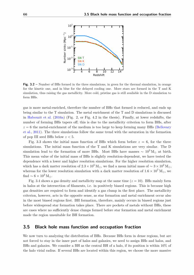
66 3.5 Black hole mass function and occupation fraction

Fig. 3.2 – Number of BHs formed in the three simulations, in green for the thermal simulation, in orangefor the kinetic one, and in blue for the delayed cooling one. More stars are formed in the T and Ksimulation, thus raising the gas metallicity. More cold, pristine gas is still available in the D simulation toform BHs.

gas is more metal-enriched, therefore the number of BHs that formed is reduced, and ends upbeing similar to the T simulation. The metal enrichment of the T and D simulations is discussedin Habouzit et al. (2016a) (Fig. 2, or Fig. 4.2 in the thesis). Finally, at lower redshifts, thenumber of forming BHs tapers off; this is due to the metallicity criterion to form BHs, afterz = 6 the metal-enrichment of the medium is too large to keep forming many BHs (Bellovaryet al., 2011). The three simulations follow the same trend with the saturation in the formationof pop III seed BHs below z < 5.

Fig. 3.3 shows the initial mass function of BHs which form before z = 6, for the threesimulations. The initial mass function of the T and K simulations are very similar. The Dsimulation lead to the formation of more BHs. Most BHs have masses ∼ 103 M at birth.This mean value of the initial mass of BHs is slightly resolution-dependent, we have tested thedependence with a lower and higher resolution simulations. For the higher resolution simulation,which has a dark matter resolution of 2.3× 105 M, we find a mean initial mass of ∼ 3× 102 M,whereas for the lower resolution simulation with a dark matter resolution of 1.6× 107 M, wefind ∼ 6× 103 M.

Fig. 3.4 shows a gas density and metallicity map at the same time (z = 10). BHs mainly formin halos at the intersection of filaments, i.e. in positively biased regions. This is because highgas densities are required to form and identify a gas clump in the first place. The metallicitycriterion, however, acts in the opposite sense, as star formation and metal enrichment occur alsoin the most biased regions first. BH formation, therefore, mainly occurs in biased regions justbefore widespread star formation takes place. There are pockets of metals without BHs, theseare cases where no sufficiently dense clumps formed before star formation and metal enrichmentmade the region unsuitable for BH formation.

3.5 Black hole mass function and occupation fraction

We now turn to analyzing the distribution of BHs. Because BHs form in dense regions, but arenot forced to stay in the inner part of halos and galaxies, we need to assign BHs and halos, andBHs and galaxies. We consider a BH as the central BH of a halo, if its position is within 10% ofthe halo virial radius. If several BHs are located within this region, we choose the more massive

Pop III remnants and stellar clusters 67

Fig. 3.3 – Initial mass function of BHs for the D (blue), K (orange), and T (green) simulations. Theinitial mass function of the T and K simulations are very similar. The D simulation leads to the formationof more and more massive BHs.

as the central BH. For galaxies, we proceed in the same way, looking for BHs inside the virialradius of galaxies (with a lower limit of 4 × ∆x).

Fig. 3.5 shows the cumulative mass function of BHs at different redshifts. This differs fromthe initial mass function of BHs (Fig. 3.3), as we take into account both the seed mass, the massaccreted by the BHs and BH-BH mergers (which are sub-dominant in the mass growth budget).We show in Fig. 3.5 the three different simulations, with the thermal, kinetic, and the delayedcooling SN feedbacks.

The evolution with time is as expected: with increasing cosmic time (decreasing redshift),more and more BHs form, and the already formed BHs grow in mass. Although the massfunctions are very similar for the T and K simulations, the low-mass and high-mass ends slightlydiffer. More central BHs are identified in the kinetic feedback simulation. The high-mass end ofthe distribution is higher in the T case, showing that the weak thermal SN feedback favours thegrowth of BHs. The delayed cooling simulation has the largest number of BHs. Conversely, theBHs do not grow in mass as efficiently as in the T and K simulations. The strong SN feedbacklimits the growth of BHs. In summary, BHs are more numerous in the delayed cooling SNfeedback simulation, but their masses are smaller. Only few BHs reach a final mass of 106 M byz = 3 with a strong delayed cooling SN feedback. In the T simulation, because the SN feedbackis weaker, BHs can grow faster to even higher mass (several BHs reach 107 M by z = 3). Theimpact of SN feedback is discussed in more details in Section 3.6.

Our BH formation model does not necessarily place a BH in each and every galaxy. Oneof the diagnostics to distinguish between BH formation scenarios, in fact, is the probabilitythat a galaxy or a halo hosts a BH: the occupation fraction. Theoretical studies predict adifferent occupation fraction of halos for different models, especially in low-mass galaxies andhalos. Observing a large sample of low-mass galaxies, and measuring the eventual mass of thecentral BH will therefore provide constrains on scenarios.

We show in Fig. 3.6 the halo mass function at different redshifts, where we show both thetotal mass function, and the mass function of halos hosting a BH. As discussed in the previoussection, BH formation occurs in the most biased halos first (Bellovary et al., 2011). BH formation,however, does not occur in all halos. Large haloes have a higher probability of hosting a BH,whereas this probability drops significantly for low-mass haloes. For the D simulation, the

68 3.5 Black hole mass function and occupation fraction

Fig. 3.4 – Gas density (left) and metallicity (right) maps at z ∼ 10 for the delayed cooling SN feedbacksimulation. BHs are highlighted with circles, circle sizes are proportional to BH masses. BH formationwalks a fine line: the necessity of having high gas densities selects biased regions, the criterion of low-metallicity works in the opposite way. BHs form in biased regions just before they experience a starformation event.

Pop III remnants and stellar clusters 69

Fig. 3.5 – Cumulative BH mass function for the thermal SN feedback simulation (T, top panel), thekinetic one (K, middle panel), and for the delayed cooling one (D, bottom panel), for redshift z = 8, 6, 5, 4.Less BHs are produced in the T and K simulations, but they grow more, up to ∼ 107M, about one orderof magnitude higher than for the delayed cooling one, which is a signature of SN feedback regulating thegrowth of low mass BHs in the case of strong feedback (delayed cooling).

70 3.6 Black hole growth regulated by efficient SN feedback

Fig. 3.6 – Total halo mass function (black; shaded areas represent poissonian error bars). The massfunction of halos hosting BHs are shown in colours (green for simulation T, orange for K, and blue for D;shaded areas also represent poissonian error bars).

occupation fraction is above 50% only for haloes more massive than 109.5 M, or galaxies withstellar mass above 107.2 M. For the T and K simulations, an occupation fraction of 50% is foundfor higher haloes (1010.5 M) and galaxy masses (galaxies with stellar mass above 108.8 M). Themass function of haloes hosting a BH is closer to the total halo mass function for the delayedcooling simulation since more BHs form in this simulation.

We show in Fig. 3.7 the BH occupation fraction as a function of galaxy mass. Here again, theprobability for galaxies to host a BH is high at the high-mass end of galaxies, and drops at thelow-mass end. At fixed galaxy mass, the occupation fraction is higher for the simulation withthe delayed cooling SN feedback, for two reasons. First, because it allows the formation of moreBHs, and second, because the strong SN feedback reduces the galaxy stellar mass, therefore theoccupation fraction is shifted compared to the other simulations T and K, which have a weakerSN feedback. Regarding the evolution with redshift, the galaxy occupation fraction can increaseby mergers of galaxies, and the formation of new BHs. As we have seen that no new BHs areformed since z ∼ 5, and mergers are few, the evolution with redshift can be explained by thegrowth in mass of galaxies. At a given galaxy mass, the occupation fraction is lower at lowerredshift, because galaxies have grown in mass. The lower redshift occupation fraction is shiftedto higher galaxy masses. This occupation fraction can be used to seed with BHs cosmologicalsimulations at lower resolution, which can not resolve the small galaxies where BHs are expectedto form.

3.6 Black hole growth regulated by efficient SN feedback

Most BHs in our simulations are growing slowly. The normalized histograms of the BH accretionrate for the three simulation are shown in Fig. 3.8. We have averaged the histogram over fewoutputs around z = 4. The typical accretion rate for the D simulation is highly sub-Eddington.In the kinetic and thermal SN feedback simulations, instead, a significant fraction of the BHs are

Pop III remnants and stellar clusters 71

Fig. 3.7 – Probability that a galaxy of a given mass at a given redshift hosts a BH. This occupationfraction for the thermal (T, green), and the kinetic (K, orange) SN feedbacks is similar, and lower thanfor the delayed cooling SN feedback (D, blue). The occupation fraction for the D simulation is higherbecause more BHs are formed in this simulations compared to the others, but galaxies are also less massive,because of the stronger SN feedback. With time the occupation fraction shifts to the right because galaxiesare becoming more massive with time, but no more BHs are formed below z = 5. The number of BHsremains almost identical, but galaxies grow.

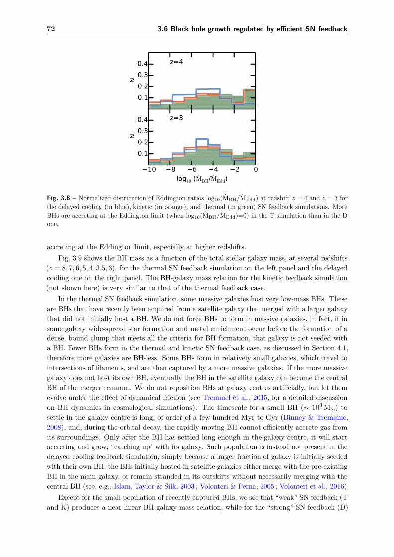
72 3.6 Black hole growth regulated by efficient SN feedback

Fig. 3.8 – Normalized distribution of Eddington ratios log10(MBH/MEdd) at redshift z = 4 and z = 3 forthe delayed cooling (in blue), kinetic (in orange), and thermal (in green) SN feedback simulations. MoreBHs are accreting at the Eddington limit (when log10(MBH/MEdd)=0) in the T simulation than in the Done.

accreting at the Eddington limit, especially at higher redshifts.Fig. 3.9 shows the BH mass as a function of the total stellar galaxy mass, at several redshifts

(z = 8, 7, 6, 5, 4, 3.5, 3), for the thermal SN feedback simulation on the left panel and the delayedcooling one on the right panel. The BH-galaxy mass relation for the kinetic feedback simulation(not shown here) is very similar to that of the thermal feedback case.

In the thermal SN feedback simulation, some massive galaxies host very low-mass BHs. Theseare BHs that have recently been acquired from a satellite galaxy that merged with a larger galaxythat did not initially host a BH. We do not force BHs to form in massive galaxies, in fact, if insome galaxy wide-spread star formation and metal enrichment occur before the formation of adense, bound clump that meets all the criteria for BH formation, that galaxy is not seeded witha BH. Fewer BHs form in the thermal and kinetic SN feedback case, as discussed in Section 4.1,therefore more galaxies are BH-less. Some BHs form in relatively small galaxies, which travel tointersections of filaments, and are then captured by a more massive galaxies. If the more massivegalaxy does not host its own BH, eventually the BH in the satellite galaxy can become the centralBH of the merger remnant. We do not reposition BHs at galaxy centres artificially, but let themevolve under the effect of dynamical friction (see Tremmel et al., 2015, for a detailed discussionon BH dynamics in cosmological simulations). The timescale for a small BH (∼ 103 M) tosettle in the galaxy centre is long, of order of a few hundred Myr to Gyr (Binney & Tremaine,2008), and, during the orbital decay, the rapidly moving BH cannot efficiently accrete gas fromits surroundings. Only after the BH has settled long enough in the galaxy centre, it will startaccreting and grow, “catching up" with its galaxy. Such population is instead not present in thedelayed cooling feedback simulation, simply because a larger fraction of galaxy is initially seededwith their own BH: the BHs initially hosted in satellite galaxies either merge with the pre-existingBH in the main galaxy, or remain stranded in its outskirts without necessarily merging with thecentral BH (see, e.g., Islam, Taylor & Silk, 2003 ; Volonteri & Perna, 2005 ; Volonteri et al., 2016).

Except for the small population of recently captured BHs, we see that “weak” SN feedback (Tand K) produces a near-linear BH-galaxy mass relation, while for the “strong” SN feedback (D)

Pop III remnants and stellar clusters 73

the BH-galaxy mass relation plateaus at low galaxy mass with an ankle at M∗ = 109 − 1010 Mand a steep rise above this mass transition. BHs grow faster (see Fig. 3.8) in the T and Ksimulations than in the D simulation, and as a result the BH masses are larger relative to theirgalaxy stellar mass. This mechanism was identified in Dubois et al. (2015) as the SN-regulatedgrowth of BHs in low-mass galaxies by means of one single zoom cosmological simulation ofgroup progenitor at z = 2. We, here, confirm the result with a statistical sample of high-redshiftgalaxies.

The kinetic and thermal feedbacks are weaker, because the energy released by the SN explosionis distributed in the nearby surrounding cells, however, the cold gas present in dense regionscentral regions is not destroyed (because of short cooling times) and is still available to formstars, BHs, and also to fuel an existing BH. Dubois et al. (2015) find that this cold gas reservoirfuels the BH efficiently, and accretion occurs at rates close to the Eddington limit. In contrast,with delayed cooling SN feedback, the dense gas clumps in star-forming regions are destroyed bythe release of energy after a SN explosions with a SN wind velocity of around 270 km s−1. Themain effect is to reduce the BH growth (and star formation) in the central regions of the galaxyby routinely removing the dense star-forming gas with SN winds, until the gravitational potentialwell of the bulge and galaxy is deep enough to confine the cold gas close to the BH. Dubois et al.(2015) show that the growth of the rest of the galaxy is not much impacted (though growing at aslower rate than with inefficient SN feedback), therefore the total stellar mass keeps growing butnot the BH mass, nor the bulge mass. It is only when the galaxy mass and bulge stellar massbecome massive enough (i.e. with a corresponding escape velocity larger than SN-wind velocity)that the BH can proceed to a rapid near-Eddington growth only altered by the self-regulationdue to AGN feedback. They measured that this transition occurred for a galaxy stellar mass of109 − 1010 M (corresponding to vesc = 300− 400 km s−1).

In Fig. 3.9 we report also the BH and stellar mass for the objects published by Reines &Volonteri (2015) (dark and light blue points). In this paper, 262 broad-line AGN and 79 galaxieswith dynamical BH mass measurement, for redshift z < 0.055, are used to investigate the scalingrelation between BH mass and the total stellar mass of galaxies. We see that when BHs grow,they eventually connect to the low-redshift sample. In low-mass galaxies, however, BHs areunable to grow, and more so if SN feedback is strong, and BHs remain “stuck" at low mass.Volonteri & Stark (2011) proposed, based on empirical arguments, that if BHs in small galaxiesare under-massive and BHs in large galaxies are over-massive, then one can reconcile severalobservational results, namely that analysis of the BH mass/luminosity function and clusteringsuggests that either many massive galaxies do not have BHs, or these BHs are less massive thanexpected (Willott et al., 2010a ; Treister et al., 2013 ; Weigel et al., 2015).

To investigate BH growth in more detail, we track the BHs with mass above 106 M at z = 3.The thermal SN feedback simulation has 24 BHs above this mass threshold, the kinetic one 22,and the delayed cooling one only 2. In Fig. 3.10, we show the growth of these BHs with solid lines(left panel for the simulation with the thermal SN feedback, right panel for the delayed coolingone), the theoretical evolution of a BH at the Eddington limit is also showed with a dashed line.All BHs in the thermal and kinetic SN feedback simulations have episodes of accretion at theEddington limit. In contrast, the growth of BHs in the delayed cooling simulation is smoother,and Eddington-limited phases minimal in particular at early times.

74 3.6 Black hole growth regulated by efficient SN feedback

Fig. 3.9 – BH mass as a function of the total galaxy stellar mass for the kinetic SN feedback (left) andthe delayed cooling SN feedback (right). BHs in the smallest galaxies have a very hard time to growbecause low-mass galaxies have shallow potential wells, and supernova feedback is sufficient to energizegas and suppress BH accretion.

Fig. 3.10 – We show here the BH growth of the most massive BHs, MBH > 106 M at z = 3, for thesimulation with thermal SN feedback (left panel) and the one with the delayed cooling SN feedback (rightpanel). The dashed line represents BH growth at the Eddington limit. For the thermal feedback, BHsgrows rapidly with several episodes at the Eddington limit, whereas for the delayed cooling SN feedbacksimulation, BH growth is smoother. Only two BH in this simulation succeed in growing to 106 M byz = 3. We do not show the corresponding plot for the simulation with kinetic SN feedback; it is verysimilar to the thermal SN feedback simulation.

Pop III remnants and stellar clusters 75

3.7 Comparisons with a sample of local galaxies, and Lyman-BreakAnalogs

Over the past decades, an incredible effort has been made to study, theoretically and obser-vationally, the BH, quasars and AGN population in massive galaxies, very often looking forthe smoking gun of AGN feedback, thought to impacting the growth and star formation at thehigh-mass end of the galaxy distribution. In Fig. 3.11 we present the luminosity function of BHsat different redshifts, and compare it to the fit to the bolometric luminosity function compiled byHopkins, Richards & Hernquist (2007) and its extrapolation (middle and bottom panels on theleft in Fig. 3.11), and to the X-ray luminosity (middle and bottom panels on the right, Buchneret al. (2015)). Our low-mass, slowly accreting BHs are well below current observational limits.Future high-sensitivity missions, such as JWST and ATHENA, and proposed ones such as X-raySurveyor and StarX, can instead start probing the luminosity range where normal high-z BHs innormal galaxies are evolving, instead of the brightest quasars powered by the most massive BHswe can reach today.

The high-mass end of the BH distribution provides us essential information on the growth ofBHs. However, as the host galaxies are typically massive, all the clues relating to BH formationhave been erased by the growth of BH, through gas accretion and BH-BH mergers (e.g., Dubois,Volonteri & Silk, 2014, and references therein). In order to collect crucial information on BHformation, one has to look at the least evolved galaxies. Lacking observational samples of low-mass galaxies at high-redshift, we compare our simulations to two different types of low-redshiftgalaxies: dwarf galaxies and local analogs of high-redshift galaxies (LBAs).

In recent years, many studies have started looking for evidence of the presence of BHs inlow-mass galaxies (with stellar mass of M? ∼ 109 M): evidence for accreting BHs with broad Hαline in the SDSS survey (Greene & Ho, 2004, 2007b ; Dong et al., 2012), evidence for narrow-lineAGN in low stellar velocity dispersions (favoring the presence of a low mass BH). Reines, Greene& Geha (2013) went further and performed the first systematic search for BHs in galaxieswith stellar mass of M? < 3× 109 M. They found 136 dwarf galaxies harboring evidences ofactive BHs (photoionization signatures, broad emission lines). The comparison between ourhigh-redshift samples (from z = 8 in green to z = 3 in red points) and the observations in thelocal Universe (dark and light blue points) is shown in Fig. 3.9. We discussed how BH growthappears to be stunted in low-mass galaxies by SN winds, but with our high-redshift simulationswe can only extrapolate our results to the local Universe provided that the BH to galaxy massrelation show little-to-no evolution with redshift (e.g. Volonteri et al., 2016 for the Horizon-AGNsimulation, Dubois et al., 2014); bringing such high-resolution simulation as SuperChunky toz = 0 is computationally very expensive.

A fairer comparison can be made with local analogs of high-redshift galaxies. Such LBAs arepromising laboratories for constraining BH formation. They have properties similar to the moredistant Lyman Break Galaxies (LBGs), in terms of mass, age, size, metallicity, star formationrate, optical extinction, but are much closer to us, thus permitting more detailed studies. AGNin LBAs can then provide us crucial clues on BHs in LBGs and then directly on the high redshiftpopulation of BHs. Fig. 3.12 compares the sample of BHs in our simulations with the sampleof XMM observation of six LBAs described in Jia et al. (2011a), with z 6 0.3. We show thenormalized distribution of accretion rate, shown as X-ray luminosity. The accretion rate is similarfor the high-z galaxies for the most luminous BHs in the simulation and the LBAs (shown asblack triangles in Fig. 3.12) suggesting that the physical conditions are at least comparable.

76 3.7 Comparisons with a sample of local galaxies, and Lyman-Break Analogs

Fig. 3.11 – Luminosity function of simulated BHs, and comparison with observations. In the two toppanels, we show the evolution of the bolometric luminosity function of the simulated BHs with time (forz = 6, 4, 3) for the simulation T (top left panel) and the simulation D (top right panel). In the 4 bottompanels, we compare the bolometric (left) and the hard X-ray (right) luminosity function of simulated BHsin simulations D (blue), K (orange) ,T (green) with observations (shaded grey regions, Hopkins, Richards& Hernquist (2007), and Buchner et al. (2015)). The middle panels show the comparison at z = 5, andbottom panels at z = 3.

Pop III remnants and stellar clusters 77

Fig. 3.12 – BH hard X-ray luminosity from the simulations (delayed cooling in blue, kinetic SN feedbackin orange, thermal SN feedback in green, at redshift z = 3), compared to the observed BHs in LBAs(black triangles). The luminosity, and so the accretion rate, of the most luminous simulated BHs is similarto the LBAs, suggesting that the physical conditions are at least comparable.

78 3.8 Conclusions

3.8 Conclusions

In this chapter, we present a new implementation to seed cosmological simulations with BHs. Ourimplementation mimics BH formation models based on stellar properties, namely a scenario basedon remnants of PopIII stars, and a scenario based on stellar mergers in nuclear star clusters atlow metallicity. The seed BHs are relatively small, as expected for the scenario investigated here.Most BHs have masses ∼ 103 M at birth. The lowest mass central BH in a galaxy (ignoring“normal" stellar mass BHs) has a mass estimate of ∼ 50,000 M (Baldassare et al., 2015), andwas identified as a low-luminosity AGN in the dwarf galaxy RGG 118 (Reines, Greene & Geha,2013). Our implementation allows for such low-mass BHs to be accounted for.

This implementation is not based on halo properties, but on the local environment of theBH formation sites. The code first identifies all the local overdensities in the gas density field,selects clumps that are bound and collapsing along all axes. If the gas metallicity is below acritical value, they are flagged as potential sites for BH formation. We compute the stellar massformed in these dense regions and the probability of forming a BH, based on the IMF and thetotal stellar mass in the clump. If the stellar mass is low (< 103 M) the probability of forminga BH is less than unity. Once a region is flagged as a site for BH formation, the mass of the BHis computed, directly related to the stellar mass. Therefore each BH in the simulation box has adifferent mass, assigned on-the-fly. To mimic the formation of these BHs, we use sink particles,which are able to accrete gas from their surroundings, and to merge together.

SN feedback is of paramount importance, as it modulates metal enrichment, as well as thepresence and retention of cold gas in low-mass galaxies. We compare three implementations ofSN feedback: one of the simulations uses a thermal feedback, another one a kinetic feedback,while the last one uses a delayed cooling feedback. Our main results are as follows.

• We find that a stronger SN feedback, delayed cooling, produces galaxies with stellar massescloser to those predicted by the relation with halo mass.

• We find that with strong SN feedback, more BHs are formed, but their growth is SN-regulated for low-mass galaxies with M∗ < 109 M (Dubois et al., 2015): SN-driven windsremove dense star-forming gas and stunt BH accretion in galaxies with shallow potentialwells.

• The lower BH masses and lower accretion rates predicted by the simulation with thestrongest SN feedback, delayed cooling, seem to be in better agreement with the paucity ofAGN in high-z galaxies (Weigel et al., 2015 ; Cappelluti et al., 2016, and references therein).

• We provide the probability that a galaxy of a given mass and redshift hosts a BH (Fig. 3.7).This information can be used to seed with BHs lower resolution cosmological simulations.

• The occupation fraction is also used as a diagnostic of BH formation. Our results agreewith analytical and semi-analytical studies (Volonteri, Lodato & Natarajan, 2008 ; vanWassenhove et al., 2010 ; Devecchi et al., 2012) and with the simulations by Bellovaryet al. (2011), in that all high-mass haloes/galaxies tend to host a BH, but low-masshaloes/galaxies have a lower probability of hosting a BH. After BH formation stops atz ∼ 6, at a given galaxy mass the occupation fraction decreases with time because galaxiesgrow in mass. We provide the occupation fraction at high redshift, when the diagnosticis for today’s low mass galaxies, however low mass galaxies are expected to experiencea quieter merger history, and therefore the occupation fraction for low-mass galaxies is

Pop III remnants and stellar clusters 79

not expected to vary much from high redshift to z = 0. One caveat is that our predictedoccupation fraction slightly depends on the resolution of the simulations, but the modelswe provide is in good agreement with several observations, such as the bolometric and x-rayBHs luminosity function, and the number of AGN candidates identified at high redshift inthe CDF-S survey.

• We have compared the BH populations from our simulations to a sample of galaxiesrepresentative of the local Universe (Reines & Volonteri, 2015) and to LBAs, local analogsof high-redshift LBGs (Jia et al., 2011a). Our simulated BHs connect to the low-redshiftobservational sample, and span a similar range in accretion properties as LBAs.

3.9 Perspectives: the details of BH growth, and predictions for fu-ture observations

3.9.1 BH growth in the delayed cooling SN feedback simulation

In the strongest SN feedback simulation presented in this chapter, those with delayed cooling, wehave seen that early BHs growth is regulated by SN feedback. Some of the BHs in the simulationbox, however, are still able to growth up to ∼ 106 M. What physical process allows some BHsto grow and others to be left behind?

Fig. 3.13, 3.14, and 3.15 show the mass evolution of three BHs (see bottom panels) overcosmic time. Black arrows represent the time at which we show the gas density maps (a,b,c,d,e,f),before and after a high accretion episode. From these figures, it seems that in most of the cases agalaxy merger triggers the episode of high accretion into the BHs. This may imply a dynamicaleffect, i.e. torques feeding the BH with gas on timescales shorter than star formation, or that thegalaxy bulge grows sufficiently to reach the mass needed to retain gas, as suggested by Duboiset al. (2015). We are planning to study in more detail the growth of these BHs, and the evolutionof the host galaxies, such as the evolution of star formation, for example.

3.9.2 Need for further comparisons with observations, preparing future observa-tional missions.

Comparisons with observationsThe comparison with LBAs so far only includes 5 LBAs (Jia et al., 2011b), and we span a similarrange in accretion properties as LBAs. We are lacking of statistics, so we would like to workclosely with observers to pursue our comparisons with larger sample of LBAs.I also want to investigate in more detail the population of BHs in LBGs. Generally very fewAGNs are observed in these galaxies. The identification of AGN in LBGs is difficult even forthose that show some AGN signatures, e.g. the detection of CIV or HeII can hint either alow-luminosity AGN, as well as a population of hot young stars (Stark et al., 2015 ; Pallottiniet al., 2015), the same problem is observed for LBAs (Jia et al., 2011b). Indeed these galaxiesoften show evidences for composite system, intense starburst or/and obscured AGN, making theAGN signatures questionable. With my simulation, I would like to predict the number of BHs inLBGs, and using theoretical spectra (Feltre, Charlot & Gutkin, 2016), estimate the optical andX-ray signal over star formation rate. It will help us to understand why AGN have not beenobserved so often in LBGs. BHs in these galaxies could be absent, or at least very faint andtherefore not easily observable. In the simulation SuperChunky D, we have indeed see that BHsare stuck at low mass, the growth is stopped partly because of the feedback from supernovae,

80 3.9 Perspectives

a b

cd

e f

Fig. 3.13 – Black hole growth of one of the most massive BH at z = 3. Panel a,b,c,d,e,f show gas densitymaps centered on the BH position (black point), the figures represent 0.5 cMpc around the BH, colorbarranges in 10−5 − 10 H/cc. The bottom panel shows the evolution of the BH mass through cosmic time.Black arrows indicate the corresponding gas density map panels.

Pop III remnants and stellar clusters 81

a b c d e f

Fig. 3.14 – Black hole growth of one of the most massive BH at z = 3. Panel a,b,c,d,e,f show gas densitymaps centered on the BH position (black point), the figures represent 0.5 cMpc around the BH, colorbarranges in 10−5 − 10 H/cc. The bottom panel shows the evolution of the BH mass through cosmic time.Black arrows indicate the corresponding gas density map panels.

82 3.9 Perspectives

a b c d e f

Fig. 3.15 – Black hole growth of one of the most massive BH at z = 3. Panel a,b,c,d,e,f show gas densitymaps centered on the BH position (black point), the figures represent 0.5 cMpc around the BH, colorbarranges in 10−5 − 10 H/cc. The bottom panel shows the evolution of the BH mass through cosmic time.Black arrows indicate the corresponding gas density map panels.

Pop III remnants and stellar clusters 83

Fig. 3.16 – Figures from Fransceca Civano (adapted from Civano et al. (2015)). The left panel showsall the different X-rays surveys, and the new surveys ATHENA and X-ray Surveyor, which will pushobservations to much deeper sources. The right panel shows in blue lines the number of observable BHspredicted from my simulation Chunky (previous version of the simulations shown in this chapter) andHorizon-AGN (Volonteri et al., 2016), the black line shows again the X-ray Surveyor survey.

which could lead to a faint population of BHs in LBGs/LBAs.

Predictions for future missionsFig. 3.16 (left panel, adapted from Civano et al. (2015)) shows the diversity of already exist-ing X-ray missions, and the upcoming or proposed X-ray missions: the large X-ray telescopeATHENA and the X-ray Surveyor. I collaborated with Francesca Civano and we have used mysimulations (a previous version of SuperChunky, the simulations used in this chapter) to predictthe number density of BHs observable with the X-ray Surveyor survey. The preliminary resultof this collaboration is shown in the right panel of Fig. 3.16, where the black line refers to theX-ray mission, and the blue lines to the prediction of observable BHs from my simulation (forhigh resolution) and the simulation Horizon-AGN of Yohan Dubois (for a lower resolution, seeVolonteri et al., 2016).

84 3.9 Perspectives

Chapter 4Direct collapse model

Supermassive BHs reside in the center of most local galaxies, but they also power active galacticnuclei and quasars, detected up to z = 7. These quasars put constraints on early BH growth andthe mass of BH seeds. The scenario of “direct collapse” is appealing as it leads to the formation oflarge mass BH seeds, 104 − 106M, which eases explaining how quasars at z = 6− 7 are poweredby BHs with masses > 109 M. Direct collapse, however, appears to be rare, as the conditionsrequired by the scenario are that gas is metal-free, the presence of a strong photo-dissociatingLyman-Werner flux, and large inflows of gas at the center of the halo, sustained for 10− 100 Myr.We performed several cosmological hydrodynamical simulations that cover a large range of boxsizes and resolutions, thus allowing us to understand the impact of several physical processeson the distribution of direct collapse BHs. We identify halos where direct collapse can happen,and derive the number density of BHs. We also investigate the discrepancies between hydro-dynamical simulations, direct or post-processed, and semi-analytical studies. Under optimisticassumptions, we find that for direct collapse to account for BHs in normal galaxies, the criticalLyman-Werner flux required for direct collapse must be about two orders of magnitude lower thanpredicted by 3D simulations that include detailed chemical models. However, when supernovafeedback is relatively weak, enough direct collapse BHs to explain z = 6− 7 quasars can be ob-tained for Lyman-Werner fluxes about one order of magnitude lower than found in 3D simulations.

This chapter is adapted from its corresponding publications, the chapter follows mostly the firstpublication:

• On the number density of "direct collapse" black hole seeds,Mélanie Habouzit, Marta Volonteri, Muhammad Latif, Yohan Dubois, and SébastienPeirani,MNRAS, 2016, vol 463, pages 529-540, arXiv:1601.00557

• Impact of dust cooling on direct collapse black hole formation,Muhammad Latif, Kazuyuki Omukai, Mélanie Habouzit and Dominik Schleicher, andMarta Volonteri,ApJ, 2016, vol 823, page 40, arXiv:1509.07034

85

86 4.1 Introduction

Contents4.1 Introduction . . . . . . . . . . . . . . . . . . . . . . . . . . . . . . . . . 864.2 Simulation set up . . . . . . . . . . . . . . . . . . . . . . . . . . . . . . 894.3 Method . . . . . . . . . . . . . . . . . . . . . . . . . . . . . . . . . . . . 924.4 Impact of SN feedback on metallicity and star formation . . . . . . 944.5 Number density of direct collapse regions in Chunky . . . . . . . . . 954.6 Horizon-noAGN simulation: Can DC model explain z = 6 quasars? 984.7 Comparison between hydro. simulations and (semi-)analytical models1014.8 Conclusions . . . . . . . . . . . . . . . . . . . . . . . . . . . . . . . . . . 1044.9 Perspectives: Applications of hybrid SAMs . . . . . . . . . . . . . . . 107

4.1 Introduction

In the last chapter, we have investigated two BH formation models, PopIII remnants and stellarclusters, which are predicted to form light BH seeds. The direct collapse model, instead, predictthe formation of more massive BH seeds, of 104−106 M seeds, making it easier to reproduce thequasar population at z > 6. As we have said in the introduction of this thesis, several variants ofthe model have been studied theoretically. The direct collapse of pristine gas can be triggered bydynamical processes (Loeb & Rasio, 1994 ; Eisenstein & Loeb, 1995 ; Koushiappas, Bullock &Dekel, 2004 ; Begelman, Volonteri & Rees, 2006 ; Lodato & Natarajan, 2006 ; Mayer et al., 2010),or can be isothermal in primordial halos (Bromm & Loeb, 2003 ; Spaans & Silk, 2006 ; Dijkstraet al., 2008 ; Latif et al., 2013a). The latter has become the most popular version of the directcollapse scenario.

However, the physical conditions required by the isothermal collapse model are numerous, andmake the channel a rare event. One needs a halo that has reached the atomic cooling threshold∼ 107 − 108 M, but it is still pristine, i.e., metal-free. One needs that the molecular hydrogenformation has been suppressed throughout the halo’s evolution. The two last conditions, namelythe absence of metals and molecular hydrogen, ensure that there is no efficient coolant in thegas. Conversely, the presence of metals and molecular hydrogen would decrease the temperatureof the gas, and so the Jeans mass. This could lead to the fragmentation of the gas cloud,therefore the formation of only one massive object is unlikely, and the formation of several lessmassive objects, namely PopIII stars, is instead expected. The destruction and prevention ofmolecular hydrogen can be accomplished by strong photo-dissociating radiation (Lyman-Werner,LW, photons with energy between 11.2 eV and 13.6 eV). A large inflow rate of gas at the centerof the halo, higher than 0.1 M/yr, and sustained for at least 10 Myr, is also needed to forma supermassive star-like object in the nucleus (Begelman, Volonteri & Rees, 2006 ; Begelman,Rossi & Armitage, 2008 ; Begelman, 2010 ; Ball et al., 2011 ; Hosokawa, Omukai & Yorke, 2012 ;Hosokawa et al., 2013 ; Schleicher et al., 2013). The BH mass can be up to 90% of the stellar mass.

Several aspects, on different physical scales, of the direct collapse scenario have been addressedin the last years. However, so far, studies have focused either on small scale simulations to capturethe physical processes leading to the gas collapse, or on semi-analytical studies to derive a DCBHnumber density. For instance, Latif et al. (2013a) used zoomed cosmological hydrodynamicalsimulations of single halos to show that when all the conditions listed above are met, collapse

Direct collapse model 87

can happen (see also Regan, Johansson & Wise, 2014). Agarwal et al. (2012, A12 thereafter) andAgarwal et al. (2014, A14 thereafter), investigated in post-processing spatial variations in theLW radiation and the importance of the clustering of the LW photon sources, using a 4 comovingMpc (cMpc) cosmological hydrodynamical simulation. In the meanwhile, semi-analytical studiesalso derived the number densities of DCBHs, for example Dijkstra et al. (2008, D08 thereafter)computed the probability distribution function of the LW radiation that irradiates halos atredshift z = 10, and showed that a small fraction of halos, 10−8 to 10−6, may be exposed toradiation higher than 20 times the background radiation (see also Dijkstra, Ferrara & Mesinger,2014, D14 thereafter). Inayoshi & Tanaka (2015) include the impact of X-rays, and predict adecrease in the formation rate of DCBHs per unit volume with redshift. Agarwal et al. (2015a)and Hartwig et al. (2016) use semi-analytical models with merger trees based on the ExtendedPress & Schechter formalism. Habouzit et al. (2016b) develop a hybrid model, where they “paint"galaxies, using the prescriptions of D08 and D14, over a dark matter only simulation, in order toinclude self-consistently the clustering of halos.

On the importance of using hybrid modelsWith these models has emerged the importance of several physical processes, such as metalenrichment of the medium from galactic winds (Dijkstra, Ferrara & Mesinger, 2014), and theclustering of LW photon sources (Dijkstra et al., 2008 ; Agarwal et al., 2012). These physicalaspects rely on spatial information (halo distribution) and unfortunately, can not easily betreated with pure semi-analytical models (SAMs). Pure SAMs use the formalism of the ExtendedPress-Schechter theory (for example Valiante et al., 2016), where massive halos are decomposedinto their higher redshift progenitors. The evolution of dark matter halos is followed on theirmerger tree.One key requirement for the formation of DCBHs, through isothermal collapse, is the absence ofefficient coolants within eligible DC halos, to keep the gas temperature and so the Jeans massof halos (which scales as T 3/2) high enough to avoid fragmentation. The main coolants whichoperate below Tvir = 104 K are molecular hydrogen and metals. Therefore the absence of H2is required. Nearby star-forming halos emit LW photons that are able to photodissociate H2(Omukai, 2001 ; Omukai, Schneider & Haiman, 2008 ; Shang, Bryan & Haiman, 2010 ; Latif et al.,2013a), spatial distance between halos is therefore a crucial ingredient. Cosmological simulations,either dark matter only or hydrodynamical simulations, direclty provide the separation distancebetween halos. Because DCBH regions are expected to be close to star-forming galaxies tomaintain a low abundance of H2, they are also the first regions which are exposed to metal-pollution from galactic winds driven by SNe. Metal-enrichment is predicted to be very disparatein the early Universe, but some halos could remain metal-free down to z ∼ 6 (Pallottini et al.,2014 ; Agarwal et al., 2014). The fraction of metal-free halos, or at least halos below the criticalmetallicity to avoid fragmentation, depends on chemical and mechanical processes (Schneideret al., 2006a,b). The evolution of metal-polluted bubbles escaping from halos can not be modeledeasily in pure SAMs, however cosmological hydrodynamical simulations can track self-consistentlythe evolution of metal-enrichment over the entire simulated volumes (Latif et al., 2016 ; Agarwalet al., 2014 ; Habouzit et al., 2016a). Finally cosmological hydrodynamical simulations offerthe advantage of following halo history as a function of time, which is of crucial importancefor metal pollution by heritage, for example. A good illustration of the importance of thespatial information is the scenario described in Visbal, Haiman & Bryan (2014), which recentlydiscuss the possibility of forming a DCBH in a synchronized pair halos (see also Dijkstra et al.,2008), without being metal-polluted, but while getting enough LW photons to photodissociate H2.

88 4.1 Introduction

Finally hybrid SAMs are the bridge between pure SAMs and cosmological hydrodynamicalzoom-in simulations of single halos (Latif et al., 2013a). Such small scale zoom-in simulationsare able to capture the physical processes which lead to the gas collapse. However they needto assume external quantities, such as the radiation intensity produced by nearby star-forminggalaxies. This artificial intensity is generally taken very high (about one order of magnitudehigher than what is needed in hybrid models to form a sufficient number of DCBHs) to ensure thecollapse of the gas, but may not be representative of a statistical sample. Hybrid SAMs give us theopportunity to study in more details the feasibility of the DC scenario. They provide a reasonableset of parameters, such as the probability of halos with a given angular momentum, fraction ofmetal-poor halos, radiation intensity, which can be used as inputs for zoom-in simulations, andgive us a first insight on the occurrence of zoom-in physical set up.

Current hybrid modelsThere are two types of hybrid models, those using spatial information from dark matter onlycosmological simulations, and those taking advantage of cosmological hydrodynamical simulations,which provide self-consistently information on metal pollution, star formation, and the spatialdistribution of halos. We briefly summarize here the current models that can be found in theliterature:

• Agarwal et al. (2012) use a dark matter only cosmological simulation, run in a box of4.8 cMpc side length, with a resolution of MDM ∼ 6× 103 Mh−1 ∼ 9.3× 103 M. Theyderive a number density in the range 10−2 − 10−1 cMpc−3 for Jcrit = 30 (see their fiducialmodel). The LW radiation intensity is modeled as the sum of a background intensity and alocal varying intensity, and is computed for each dark matter halos of the simulation box.

• Agarwal et al. (2014) use the same LW model as Agarwal et al. (2012), but this time ontop of a hydrodynamical simulation. The simulation FiBY is a 4 cMpc box size simulation,with a resolution of MDM ∼ 6× 103 M. The simulation FiBY includes self-consistentlyon-the-fly the treatment of H2 destruction by LW radiation, and the photo-detachmentof H−. Cooling by H2 is also included. The simulation offers the possibility to followself-consistently external metal-pollution, that was not included in Agarwal et al. (2012).The number density of DCBH regions is in the range 10−2 − 10−1 cMpc−3 for Jcrit = 30.

• Habouzit et al. (2016b) use two different dark matter only cosmological simulations of sizelength each, to study the impact of primordial non-Gaussianities in the density field on thenumber density of DCBHs. A model for LW radiation intensity is used on top of thesesimulations, and is based on Dijkstra, Ferrara & Mesinger (2014). The analysis is presentedin chapter 5.

• Habouzit et al. (2016a): the method and results of this study are presented in the presentchapter. The description of the 4 simulations used in this chapter, are described in thenext section.

• Chon et al. (2016) use a cosmological hydrodynamical simulation to identify the possibleDC regions, and then use zoom-in simulations to follow the dynamical evolution of theseregions to see whether they can collapse. A number of 42 regions are first identified with thelarge scale simulation, out of which only 2 cases are presented as having good chance to leadto the formation of a DCBH. Therefore, the number density ranges in 10−4 − 10−3 cMpc−3

Direct collapse model 89

for Jcrit = 100 (we have averaged over ∆z = 1 the number of DCBH regions found forz = 12, 11, 9, 8, 7, see their Table 1).

In this chapter, we use a hybrid method to compute the number density of BHs in differentscale simulations, and to understand the impact of different physical processes as star formationor metal-pollution through SN feedback. Finally we also aim to discuss the discrepancies betweendifferent models that have been used to derive the number density of DCBHs, along with SAMsand hybrid models.In the following, we use a set of three different cosmological hydrodynamical simulations, withincreasing box size, allowing us to capture the physical processes on small scales in a small-volume,high-resolution simulation, to derive the number density of BHs and to test the impact of theSN feedback using a larger simulation with intermediate resolution. Finally, a large-volumesimulation, with lower resolution, Horizon-noAGN (Peirani et al, in prep), is also used to testwhether the direct collapse scenario is able to explain the population of quasars that we observeat redshift z = 6. We follow the approach introduced by D08, A12, D14 and A14 and modelthe LW radiation field on top of all the different simulations. A DCBH region finder code is ap-plied to compute the DCBH number density function on all the simulations, for different redshifts.

The chapter is organized as follows. We first describe, in section 4.2, the simulations weuse in this work, and the modeling of the LW radiation intensity, in section 4.3. In section 4.4,we investigate SN feedback and, in section 4.5 how it can alter the number density of DCBHregions derived from simulations. section 4.6 is dedicated to the simulation Horizon-noAGN,for which we derive the number density of DCBH regions, and we investigate the feasibility ofthe DC scenario for explaining the population of quasars at z = 6. In section 4.7, we explore acomparison between the different methods to derive the DCBH number density (which leadsto discrepancies of several orders of magnitude), using either semi-analytical methods, or usinghydrodynamical simulations. We summarize the results of this work in section 4.8.

4.2 Simulation set up

We have performed a set of simulations with increasing box sizes from 1 cMpc to 142 cMpc, usingthe adaptive mesh refinement hydrodynamical cosmological code ramses (Teyssier, 2002). Wesummarize in the following the main characteristics of these simulations. Table 4.1 establishes acomparison between all the simulations parameters used in this work. Fig. 4.1 shows gas densitymaps of our simulations Tiny, Chunky, and Horizon-noAGN. In the density map of Chunky(middle panel), the white square indicates the size of Tiny, and in the Horizon-noAGN map(bottom panel, only a small part of the simulation box is shown here), we show the size of thesimulation Chunky.

Simulation TinyThe smallest simulation, Tiny, is performed in a periodic box of Lbox = 1 cMpc size length with2563 dark matter particles, corresponding to a mass resolution of MDM,res = 2082 M. Thesimulation uses a Λ cold dark matter cosmology, with total matter density Ωm = 0.276, darkmatter energy density ΩΛ = 0.724, amplitude of the matter power spectrum σ8 = 0.811, spectralindex ns = 0.961, baryon density Ωb = 0.045 and Hubble constant H0 = 70.3 km s−1 Mpc−1.Simulations are run with 10 levels of refinement (`min = 8 defines the number of cells on thecoarse level, `max = 17 defines the finest level of refinement), leading to a spatial resolution of

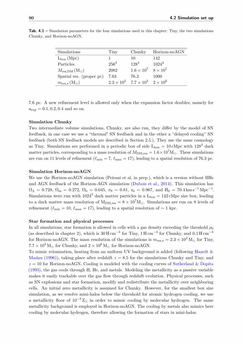
90 4.2 Simulation set up

Tab. 4.1 – Simulation parameters for the four simulations used in this chapter: Tiny, the two simulationsChunky, and Horizon-noAGN.

Simulations Tiny Chunky Horizon-noAGNLbox (Mpc) 1 10 142Particles 2563 1283 10243

Mres,DM (M) 2082 1.6× 107 8× 107

Spatial res. (proper pc) 7.63 76.3 1000mres,? (M) 2.3× 102 7.7× 103 2× 106

7.6 pc. A new refinement level is allowed only when the expansion factor doubles, namely foraexp = 0.1, 0.2, 0.4 and so on.

Simulation ChunkyTwo intermediate volume simulations, Chunky, are also run, they differ by the model of SNfeedback, in one case we use a “thermal" SN feedback and in the other a “delayed cooling” SNfeedback (both SN feedback models are described in Section 2.5.). They use the same cosmologyas Tiny. Simulations are performed in a periodic box of side Lbox = 10 cMpc with 1283 darkmatter particles, corresponding to a mass resolution ofMDM,res = 1.6×107M. These simulationsare run on 11 levels of refinement (`min = 7, `max = 17), leading to a spatial resolution of 76.3 pc.

Simulation Horizon-noAGNWe use the Horizon-noAGN simulation (Peirani et al, in prep.), which is a version without BHsand AGN feedback of the Horizon-AGN simulation (Dubois et al., 2014). This simulation hasΩΛ = 0.728, Ωm = 0.272, Ωb = 0.045, σ8 = 0.81, ns = 0.967, and H0 = 70.4 km s−1 Mpc−1.Simulations were run with 10243 dark matter particles in a Lbox = 142 cMpc size box, leadingto a dark matter mass resolution of MDM,res = 8× 107M. Simulations are run on 8 levels ofrefinement (`min = 10, `max = 17), leading to a spatial resolution of ∼ 1 kpc.

Star formation and physical processesIn all simulations, star formation is allowed in cells with a gas density exceeding the threshold ρ0(as described in chapter 2), which is 30 H cm−3 for Tiny, 1 H cm−3 for Chunky, and 0.1 H cm−3

for Horizon-noAGN. The mass resolution of the simulations is mres,? = 2.3× 102 M for Tiny,7.7× 103 M for Chunky, and 2× 106 M for Horizon-noAGN.To mimic reionization, heating from an uniform UV background is added (following Haardt &Madau (1996)), taking place after redshift z = 8.5 for the simulations Chunky and Tiny, andz = 10 for Horizon-noAGN. Cooling is modeled with the cooling curves of Sutherland & Dopita(1993), the gas cools through H, He, and metals. Modeling the metallicity as a passive variablemakes it easily trackable over the gas flow through redshift evolution. Physical processes, suchas SN explosions and star formation, modify and redistribute the metallicity over neighboringcells. An initial zero metallicity is assumed for Chunky. However, for the smallest box sizesimulation, as we resolve mini-halos below the threshold for atomic hydrogen cooling, we usea metallicity floor of 10−3 Z in order to mimic cooling by molecular hydrogen. The samemetallicity background is employed in Horizon-noAGN. The cooling by metals also mimics herecooling by molecular hydrogen, therefore allowing the formation of stars in mini-halos.

Direct collapse model 91

Fig. 4.1 – Gas density maps representing the three simulations used in this work: Tiny (Lbox = 1 cMpc,top panel), Chunky (Lbox = 10 cMpc, middle panel), and Horizon-noAGN (Lbox = 142 cMpc, here weonly show a small part of the simulation, a box of ∼ 40 cMpc side, bottom panel). The white squaresmark the size of the previous simulation: in the gas density map of Chunky (middle panel), we show thesize of Tiny, and in Horizon-noAGN map (bottom panel), we show the size of Chunky.

92 4.3 Method

The gas follow an adiabatic equation-of-state (EoS) for monoatomic gas with adiabatic indexγ = 5/3, except at high gas densities ρ > ρ0, where we use a polytropic EoS to increase the gaspressure in dense gas in order to limit excessive gas fragmentation by mimicking heating of theinterstellar medium from stars. We use the following parameters that are described in chapter 2:κ = 1.6 for the polytropic index, and T0 = 103 K for Chunky, and T0 = 102 K for Tiny. ForHorizon-noAGN, κ = 4/3 and T0 = 103 K have been used.

Supernova feedbackBecause metallicity and star formation are both a direct product of how SN feedback is modeledin hydrodynamical simulations, and are of the crucial importance when studying the directcollapse scenario, we test two different SN feedback implementations. We model SNe typeII assuming a Chabrier initial mass function, where 20% of the mass fraction of stars endup their life in type II SNe, and release 1050 erg M−1

, and return metals with a yield of 0.1.In this chapter, we use both the thermal and delayed cooling SN feedback implementations.For Chunky, we use the delayed cooling SN feedback parameters (that are described in chap-ter 2): Mgmc = 7.7 × 104 M, σNT = 4.3 × 10−4 km s−1, tdiss = 4.6 Myr. For Tiny, we use:Mgmc = 2.5 × 103 M, σNT = 2.5 × 10−4 km s−1, tdiss = 0.59 Myr. Horizon-noAGN includes a“kinetic feedback" with a strength intermediate between these two implementations.

The simulations Chunky and Horizon-noAGN do not resolve mini-halos. The impact of notresolving mini-halos in our simulations is not trivial to predict. On the first hand, we miss theearly first episode of star formation that takes place in mini-halos, and consequently the earlymetal-enrichment. Large regions can be polluted by SN feedback from PopIII star, because theirhost halos are small. In that sense, we under-estimate the pollution by metals when computingthe number of direct collapse halos. On the other hand, we also consider some halos as beingpristine when they could be polluted by metals, because we do not capture their earlier starformation episode and metal enrichment. Therefore we also over estimate in that sense thenumber of halos that are still pristine and could be eligible for the direct collapse model.

Halo catalog and merger treesWe construct catalogues of halos using the AdaptaHOP halo finder (Aubert, Pichon & Colombi,2004), which uses an SPH-like kernel to compute densities at the location of each particle andpartitions the ensemble of particles into sub-halos based on saddle points in the density field.Halos contain at least 20 particles. We study the individual evolution of halos by building mergertrees using the code TreeMaker developed by Tweed et al. (2009).

4.3 Method

We post-process the identification of all the regions, in a given simulation, which are eligible forthe formation of a DCBH. In large cosmological simulations the main difficulty is to capture bothlarge scales to have statistics and very small scales where the collapse of gas and the formationof a massive central object can be resolved. Several physical processes, playing a crucial role forthe direct collapse scenario, such as star formation, metal-enrichment, depend on the simulationresolution. In order to take this into account, we have run our DCBH finder code on threedifferent simulations. Therefore we are covering a large range of resolutions and volumes.

According to the direct collapse scenario, metal-free/metal-poor halos with mass > 107 −108 M may host DCBHs under specific conditions. An inflow rate (higher than 0.1 M/yr) of gas

Direct collapse model 93

at the center of the halo can lead to the formation of a supermassive star-like object in the nucleus.The star can then collapse and form a 105 − 106 M BH. In order for the Jeans mass to remainsufficiently high to form only one very massive object, efficient cooling by molecular hydrogen ormetals must be prevented. Therefore metal-free conditions and a strong photo-dissociating fluxare required.

A12 and A14 model the Lyman-Werner radiation as the sum of a spatial varying componentof the radiation produced by young stars and of a background component. The backgroundcomponent is described by:

JLW,bg,II = 0.3(1 + z

16

)3 ( ρ?,II10−3 M yr−1Mpc−3

)(4.1)

in units of 10−21 erg s−1 cm−2 Hz−1 sr−1, with ρ?,II = 10−3 M yr−1Mpc−3 for the star formationrate (constant with time). The background radiation intensity, however, is negligible comparedto the local radiation intensity:

JLW,local,II = 3∑

i,stars65Myr

( ri1 kpc

)−2 ( mi103 M

)(4.2)

in units of 10−21 erg s−1 cm−2 Hz−1 sr−1, with r the distance between the source and the regionwhere we compute the radiation and m the mass of the star. In the following, JLW,crit refersto the critical value of JLW,local,II in units of 10−21 erg s−1 cm−2 Hz−1 sr−1, which we simplify inJLW. In this study, as we will consider radiation intensity thresholds much above the backgroundlevel, we do not include the background component to the radiation intensity, which would benegligible compared to the spatially varying component. We have also not included radiationproduced by Pop III stars, as their contribution to DCBH formation is highly subdominantcompared to the Pop II population (see A12 and A14).

In this work, we do not include self-shielding by molecular hydrogen, self-shielding of haloscould decrease the number density of DCBH regions we find in the following sections. We donot include ionizing radiation from reionization. In the presence of an ionizing radiation beforethe beginning of the collapse of the inner part of halos, infall of gas and accretion in the centercan be decreased, which delays collapse, and triggers molecular hydrogen formation. Halos canthen reach lower temperatures, which favours star formation instead of DCBH region formation.Johnson et al. (2014) show that the fraction of halos that could experienced this process is verysmall.

The critical value required for DCBH depends of the spectrum of the stellar population,Wolcott-Green, Haiman & Bryan (2011) argue a JLW,crit = 1000 for a Pop III population, Shang,Bryan & Haiman (2010) show that the critical value ranges in JLW,crit = 30− 300 for a Pop IIpopulation. A strong radiation is needed in order to not only dissociate the molecular hydrogenin the outer parts of the halo, but also in the center. The critical values cited just above arethought to be sufficient to bring the molecular fraction down to 10−8 in 1D simulations. Thevalue of the critical radiation JLW,crit is more likely to be spread on a distribution of possiblevalues rather than equal to a fixed single value (derived from a fixed temperature black body), asshown by Sugimura, Omukai & Inoue (2014) ; Agarwal et al. (2014) ; Agarwal & Khochfar (2015).However in order to be able to compare our results on the number density of DCBH regions toprevious literature, we consider a critical value of the radiation intensity of either JLW,crit = 30(Agarwal et al., 2012, 2014), JLW,crit = 100 or JLW,crit = 300. These values are lower compared tothose required by high-resolution 3-D cosmological simulations (Regan, Johansson & Wise, 2014 ;Latif et al., 2014, 2015), which require JLW,crit > 500− 1000. Inclusion of X-rays also increases

94 4.4 Impact of SN feedback on metallicity and star formation

Fig. 4.2 – Top panel: median stellar mass enclosed in a sphere with a radius of 50 ckpc around halos(solid lines, red for the simulation with the delayed cooling SN feedback and yellow for the thermal SNfeedback). Dashed lines include only stellar mass in young stars (age 5 Myr). Bottom panel: Medianof the average metallicity of halos in the two Chunky simulations, at redshift z = 7.33, binned in mass.Shaded areas extend to the 1σ values. The spread in the metallicity, as well as in the stellar mass, isdue to very isolated halos. thermal feedback decreases the probability of having DCBH regions becausethe number of halos polluted by metals is higher, but it also favours it because the amount of radiationproduced by young stars is higher.

the critical flux (Inayoshi & Tanaka, 2015), but the net effect is still unclear (Latif et al., 2015).It will be clear in the following that if we were to consider such values we would not form anyDCBH in our volumes. In summary, what we obtain is an upper limit to the number of DCBHs,under optimistic conditions.

4.4 Impact of SN feedback on metallicity and star formation

Metals are created by stars and spread by SN explosions. Therefore SN feedback implementationhas a strong impact on the metal-enrichment of the intergalactic medium, and on the numberdensity of BH seeds formed. SN feedback also regulates star formation, therefore modulates theformation of the young stars that can provide Lyman-Werner radiation.

The simulation Tiny allows us to resolve the detailed expansion of the metal-enriched bubbles,but the size of the simulation (1 cMpc) is too small to see, statistically, the impact of SN metalenrichment on the number density of DCBHs. We use Chunky, a simulation with a side length

Direct collapse model 95

Tab. 4.2 – Number of direct collapse regions in the simulation Chunky with thermal SN feedback, assumingthat collapse requires either 10 Myr, or the full free-fall time of the halo. For reference in Chunky withdelayed cooling SN feedback, the only case that gives one candidate, at z = 7.33, has JLW,crit = 30 and acollapse time of 10 Myr.

Criteria z = 10.1 9.00 8.09 7.33JLW,crit = 30, 10 Myr 1 3 6 17JLW,crit = 30, tMyr,ff 0 0 0 3JLW,crit = 100, 10 Myr 0 0 1 3JLW,crit = 100, tMyr,ff 0 0 0 0JLW,crit = 300, 10 Myr 0 0 0 0JLW,crit = 300, tMyr,ff 0 0 0 0

10 times larger (10 cMpc), to study metal enrichment and star formation rate for a significantvolume of the Universe. We have run two identical simulations where only the prescription forthe SN feedback is different, as described in Section 4.2. The thermal SN feedback is weaker,compared to delayed cooling. In fact, the total mass in stars in the box is about one order ofmagnitude larger for the thermal feedback case, at all redshifts.

The direct collapse scenario depends on two main quantities: the metallicity of the halo, andthe radiation intensity it is exposed to, which in turn depends on the mass in nearby young stars(< 5 Myr). We compare these two quantities for the two SN feedbacks in Fig. 4.2. We calculatea halo mean metallicity averaging over all the gas leaf cells enclosed in its virial radius, and showthe median of these mean metallicity values for all the halos in the two Chunky simulations, withsolid lines in Fig. 4.2 (top panel). The shaded areas represent the 1σ values of halos metallicity.Thermal feedback leads to a higher metal enrichment. This is simply due to the larger stellarmass formed when adopting the SN thermal feedback, as evident from the bottom panel ofFig. 4.2, which represents the median stellar mass in the neighborhood of halos (solid lines), in asphere with a 50 ckpc radius. This median stellar mass is larger with the thermal feedback. Thestellar mass in young stars (6 5 Myr), which contribute at a given redshift to the LW radiation,is shown as dashed lines and follows the same trend.

It is difficult to predict the global effect of SN feedback on the number density of DCBHs ina cosmological box because metal enrichment and the amount of stellar mass in young stars haveopposite effects. Regarding the former, delayed cooling SN feedback is more favourable to theformation of DCBHs - more halos are metal-poor and therefore eligible for DCBH formation-,regarding the latter, it is the thermal SN feedback implementation that has the advantage - halosare illuminated by stronger radiation because there are more young stars at any given time.

4.5 Number density of direct collapse regions in Chunky

We now turn to identifying the number of regions which are eligible for the direct collapsescenario. These regions must fulfill three criteria: they must be metal-poor, not forming stars,and be illuminated by a LW radiation intensity higher than the threshold JLW,crit = 30 (wetake here the same value as in A12) during the whole time it takes for the collapse and DCBHformation. D08 use a free-fall time defined by:

tMyr,ff ∼ 83(1 + z

11

)−3/2, (4.3)

96 4.5 Number density of direct collapse regions in Chunky

Fig. 4.3 – We compare one DCBH candidate halo in the simulation Chunky with the thermal supernovafeedback (in orange) and the corresponding halo in the delayed cooling simulation (in red). Top panel:stellar mass (solid lines), stellar mass in young stars (dashed lines) in the neighborhood of the candidate(in a sphere of 350 ckpc radius). Bottom panel: the radiation intensity (dots) seen by the candidate halofor the two supernova feedbacks. The critical radiation intensity used in A12, JLW,crit = 30, is shown as adashed grey line. Arrows represent the free-fall time used in D08. If a candidate is above the critical LWradiation for the full length of an arrow, it is retained. In this case the orange dot (thermal feedback)remains a candidate, the red dot (delayed cooling feedback) does not.

Direct collapse model 97

which assumed ρ ∼ 200 × ρ. This is the free-fall time at the virial radius. Visbal, Haiman &Bryan (2014) argue instead that the relevant collapse time is that of the gas, on scales 10% ofthe virial radius, so that the collapse time should be 0.1× tMyr,ff . The length of the collapse in3D high-resolution simulations of Latif & Volonteri (2015), indeed lasts ∼10 Myr. In this study,we consider both the redshift-dependent collapse time, defined in Eq. 4.3 (D14), and a collapsetime of 10 Myr, which appears more realistic, according to recent simulation studies.

We give an example of our technique in the following. We show in Fig. 4.3 one concreteexample of a DCBH candidate halo, with a mass of Mh = 5.2 × 108 M at z = 7.33: the toppanel shows the evolution of the stellar mass in the environment of the halo, the total stellarmass is represented with solid lines, the stellar mass in young stars is shown with dashed lines.The corresponding radiation intensity is shown in the bottom panel with dots, the grey dashedline indicates the radiation intensity threshold of JLW,crit = 30. The simulation with thermalfeedback is shown in orange, and the simulation with the delayed cooling feedback in red. Greyarrows give an idea of the free-fall time at that redshift, computed as in D08. We see that whenthe stellar mass in young stars increases, the radiation intensity also increases, and when itdecreases at redshift z = 6.6, the radiation intensity also decreases.

Using this technique, only considering the radiation criterion, for the thermal SN feedbackcase, 17 regions are identified as potential DCBH sites, at z = 7.33. The maximum value of theradiation intensity at that redshift is JLW = 162.72. Then we look back in time using mergertrees made with TreeMaker (Tweed et al., 2009), in order to check if these candidates havebeen illuminated by a sufficiently high radiation intensity for at least one collapse time, andhow the intensity varies over time. We find that only 4 of the candidates are illuminated by aradiation intensity above the critical value for at least one collapse time, and therefore are stillflagged as DCBH candidates. Finally we check the metallicity of the candidates, and find thatonly one region is not polluted by metals, and 2 regions are partially polluted, which leads toa number density nDCBH 6 3× 10−3cMpc−3. Zero candidates are found for JLW,crit = 100 andJLW,crit = 300.

In the previous paragraph, we adopted as collapse time the free-fall time of the halo, definedby Eq. 4.3. However, if we now use a collapse time of 10 Myr, as suggested by Visbal, Haiman& Bryan (2014), for the same JLW,crit = 30, we find: 1 halo at z = 10.1 with Z < 10−3.5 Z,3 regions at z = 9.00 (all with Z = 0), 6 regions at z = 8.09 (3 regions with Z = 0, and 3regions with Z < 10−3.5 Z), 17 regions at z = 7.33 (7 regions with Z = 0, and 10 regions withZ < 10−3.5 Z). All the regions are in halos with Mh > 108 M. With a radiation intensitythreshold of JLW,crit = 100, the numbers decrease to 1 at 8.09, and 3 at z = 7.33, no DCBH halois found at z = 10.1 or z = 9.00. Zero candidates are found for JLW,crit = 300.

We repeat the same exercise for the simulation with delayed cooling SN feedback, and findonly one candidate for the DCBH process, for the case with JLW,crit = 30, and assuming a collapsetime of 10 Myr. No candidates are found in the other cases. The maximum radiation intensityis JLW = 30.33. In conclusion, the lower stellar mass in young stars in the delayed coolingsimulation directly impacts the direct collapse scenario, by strongly decreasing the number ofregions illuminated by a sufficient radiation intensity, and therefore decreasing the number densityof DCBHs. The number density of DC haloes found at a given redshift (not the cumulativenumber density) in the two Chunky boxes is shown in Fig. 4.4, with orange symbols when usingfor the collapse time the free-fall time of the halo, violet symbols for a collapse time of 10 Myr,and the number of candidates is reported in Table 4.2.

As a note, no DCBH is found in Tiny, for any subset of criteria. Tiny is the only simulationwhere we resolve minihalos, and Machacek, Bryan & Abel (2001) ; O’Shea & Norman (2008),

98 4.6 Horizon-noAGN simulation: Can DC model explain z = 6 quasars?

show that a small amount of LW flux is able to delay or temporarily shut down the formation ofPopIII stars, and instead favors the formation of second generation stars (Johnson, Dalla Vecchia& Khochfar, 2013). If we included the suppression of PopIII star formation through LW flux,this would increase the number of PopII stars, thus would increase the probability of DCBHformation. As we consider all stars as PopII stars in this work, we are already overestimatingthe LW radiation (which already mimics the enhancement of PopII formation produced bythe suppression of PopIII star formation by LW flux), thus obtaining optimistic results for theoccurrence of DCBHs. Since, under optimistic assumptions, we find zero DCBH candidates inTiny, we expect that including the suppression of Pop III star formation in pristine minihaloeswould not change strongly this null result.

Small simulation boxes only allow us to derive a number density of DCBH regions forJLW,crit = 30, which appears to be sightly lower than the values derived by D14 or A12, and evenlower compared to A14. The differences between implementations causing these discrepancies areanalyzed and discussed in Section 4.7. We will only consider the fiducial models of these studies,which are comparable to our study, with an escape fraction of unity, and no additional physicalprocesses, as the effect of galactic winds (D14) or reionization feedback (A12). A12 discuss acase with an additional reionization feedback from hydrogen-ionizing photons (however, withan escape fraction of 0.5, which differs from the other studies and makes a direct comparisonproblematic), which can strongly decrease the number density by a factor of ∼ 15 (from a numberdensity of 0.518 cMpc−3 to 0.035 cMpc−3).All the regions that we describe above are in halos with Mh > 108M. In Chunky we do notresolve smaller halos that could be still metal-poor, and available to form a DCBH region, neitherto capture the early metal-enrichment of the DCBH regions we have identified.

4.6 Horizon-noAGN simulation: Can direct collapse explain the BHspowering z = 6 quasars?

We now turn to exploring the number density of BHs in the Horizon-noAGN simulation. Thissimulation allows us to look at DCBH formation without being biased by the feedback of pre-existing BHs, compared to the sister simulation, Horizon-AGN, which includes BH accretion andfeedback. The main advantage of the simulation is that the large box (142 cMpc side length)allows some statistics, at the expense of spatial and mass resolution. We use the same method asfor the set of Chunky simulations to compute the radiation intensity illuminating halos.

We first flag all halos illuminated by a radiation intensity higher than JLW,crit = 30. Weidentify 8 regions at redshift z = 9.83, and 814 regions at z = 7.31. Since we are trying toestimate whether DCBHs can explain the number density of z > 6 quasars, we do not need toproceed to lower redshift (the next available output is at z = 5.87). This simulation includes ametallicity floor, therefore we rescaled the metallicity accordingly. Halos with a mean metallicitylower than 10−3.5Z are kept as DCBH candidates. We are left with 2 regions at redshift z = 9.83,373 regions at z = 7.31. For a radiation intensity of JLW,crit = 100 we identify 2 regions atredshift z = 9.83 and 153 at z = 7.31. Including the metallicity criterion (Z 6 10−3.5Z), thereare 0 regions at redshift z = 9.83, and 42 at z = 7.31. For a radiation threshold of JLW,crit = 300we identify 1 region at redshift z = 9.83 and 13 regions at z = 7.31. Including the metallicitycriterion, we find 0 regions at redshift z = 9.83, 2 regions at z = 7.31 (Z 6 10−3.5Z), and noregion at z = 9.83. See Table ?? for a summary. Metallicity appears to be a key parameter inthe direct collapse scenario, reducing significantly the number of DCBH candidates (up to 25 %at z = 9.83, 45 % at z = 7.31).

Direct collapse model 99

Fig. 4.4 – Number density of halos that can host a DCBH, at a given redshift. To be consistent withprevious literature, we show the number density of DCBH regions at a given redshift, this is not acumulative number density in the sense that we do not add the regions found at higher redshifts. Ingrey we show the number density from previous studies. Symbols represent different radiation intensitythresholds. Squares: JLW,crit = 30, circles: JLW,crit = 100, triangles: JLW,crit = 300. The top light greycrossed square at z = 10.5 is from A14 (post-processing of a hydrodynamical simulation), the light greysquares in the range z = 10− 7 are from A12 (values from private conversation, semi-analytical study),dark grey squares are the results of D14 (analytical). We do not show the number density derived in D08,which is in the range 10−6 − 10−8 cMpc−3, similar to the one derived in D14. The orange square showsthe number density for Chunky (10 cMpc side box), for the thermal SN feedback (0 regions are identifiedin the simulation employing the delayed cooling SN feedback), for halos that are illuminated by a highradiation intensity for at least their free-fall time. The purple squares and circles show the number densityfor Chunky, for halos that are illuminated by a high radiation intensity for at least 10 Myr. The bluesquares, circle and triangle represent the large-scale cosmological simulation Horizon-noAGN (142 cMpcside box).

Tab. 4.3 – Number of direct collapse regions in the simulation Horizon-noAGN.

Criteria z = 9.83 z = 7.31JLW,crit = 30 8 814JLW,crit = 30, Z 10−3.5Z 2 373JLW,crit = 100 2 153JLW,crit = 100, Z 10−3.5Z 0 42JLW,crit = 300 1 13JLW,crit = 300, Z 10−3.5Z 0 2

100 4.6 Horizon-noAGN simulation: Can DC model explain z = 6 quasars?

It is important to notice here that the time-scale between two outputs in the simulation arelarger than the collapse time, either the free-fall time or 10 Myr. Therefore we are missing the timecriterion of the direct collapse here: some of the candidates identified could be polluted by metalsbefore the full collapse time has elapsed and therefore before unable to form the DCBH. Theradiation intensity could also vary and not be enough to sustain molecular hydrogen dissociationfor the full collapse time. Another important caveat is the resolution of the simulation, ∆x = 1kpcand MDM,res = 8× 107 M, which does not allow us to capture the first metal-enrichment ofhalos, simply because we do not resolve small halos. Rather than the quantitative numbers,Horizon-noAGN allows us to explore trends in a statistical sense.

Fig. 4.4 shows the number density obtained for the simulation Chunky (in orange, and violet)and Horizon-noAGN (in light blue). All the grey symbols represent previous studies: the lightgrey top crossed square is for A14, the light squares for A12, dark grey squares for D14, bothfor JLW,crit = 30, dark grey circles are for D14 and JLW,crit = 300, dark grey triangles for D14and JLW,crit = 300. We do not show the number density derived in D08 (10−6 − 10−8 cMpc−3),because similar to the one obtained in D14.

In Horizon-noAGN, considering the metallicity threshold Z 6 10−3.5 Z, we find nDCBH '10−7 cMpc−3 at z = 9.83, and nDCBH ' 10−4 cMpc−3 at z = 7.31 (blue squares in Fig. 4.4), forJLW,crit = 30. At z = 7.31, for JLW,crit = 100, we find nDCBH ' 10−5 cMpc−3 (blue circle inFig. 4.4), and nDCBH ' 10−6 cMpc−3 for JLW,crit = 300 (blue triangle in Fig. 4.4).

For Horizon-noAGN, our attempt was to see if the conditions on metallicity and on radiationintensity could be meet in more than few halos. Of course, with this simulation, we do not resolvesmall halos, nor the early metal-enrichment, but it gives us a first picture of the feasibility of thedirect collapse scenario on a cosmological scale. For JLW,crit = 30, we again find a number densitysmaller than D14, and A14. However, for the highest thresholds, JLW,crit = 100, JLW,crit = 300,the number density of DCBH regions are very similar to those found by D14.

Finally, we investigate the probability for massive halos at z ∼ 6 to be seeded by a DCBH. Amassive halo at z ∼ 6, will host a DCBH if at least one of its progenitors was a DCBH region(namely metal-poor halos, illuminated by a strong photo-dissociating radiation intensity). Westart by selecting all the most massive halos in the simulation Horizon-noAGN at z = 5.8, namelythe 552 halos with Mh > 1011 M. We build the merger history of all these halos with TreeMaker(Tweed et al., 2009), with the two previous snapshots of the simulation, at z = 7.3 and z = 9.8.We compute the mean metallicity of all the progenitors of massive halos at z = 5.8, and thephoto-dissociating radiation they are illuminated by. Of the 552 halos with Mh >= 1011 M atz = 5.8, 155 have at least one DCBH progenitor at z = 7.3, illuminated by a radiation with anintensity higher than JLW,crit = 30 and with a metallicity Z < 10−3.5 Z. We do not identify anyDCBH progenitor at z = 9.8. Therefore the fraction of massive halos which can host a DCBH is155/552=0.28, so 28% of the massive halos. When considering a radiation intensity thresholdof JLW,crit = 100, only 6.5% of the massive halos can host a DCBH, and it drops to 0.36% forJLW,crit = 300.

In summary, about a third of the most massive halos at z = 6 have at least one progenitorreaching both the criterion on metallicity (Z < 10−3.5 Z) and the criterion on radiation intensity(JLW,crit = 30). However, this fraction drops significantly down to ∼ 6% for JLW,crit = 100, andeven more, down to less than 1% for a more realistic value of JLW,crit = 300.

Direct collapse model 101

Tab. 4.4 – Percentage of massive halos with at least one DCBH progenitor, in the simulation Horizon-noAGN.

Criteria Z 6 10−3.5

JLW,crit = 30 28%JLW,crit = 100 6.5%JLW,crit = 300 0.36%

4.7 Comparison between hydro-dynamical simulations and(semi-)analytical models

In this section, we perform a systematic comparison between different models presented in theliterature. Analytical and semi-analytical studies have the advantage of investigating with easethe impact of physical processes. Ahn et al. (2008) show that the clustering of halos, which arethe sources responsible for the photo-dissociating background, leads to local variations in theLW radiation intensity background. D14 uses a semi-analytical model to investigate the roleof galactic outflows, which drive metal-enrichment in the surrounding of star-forming galaxies.DCBH regions need to be close enough to star-forming galaxies in order to be illuminated bya high radiation intensity, whereas the proximity with star-forming regions imply a potentialmetal-pollution by their galactic winds. Agarwal et al. (2012) and Habouzit et al. (2016b) use ahybrid model where they “paint” galaxies on dark matter only simulations, so that the clusteringof halos is naturally taken into account.

Conversely, hydrodynamical simulations have the advantage of tracking the cosmic evolutionof metal-enrichment and star formation in a more self-consistent way, where semi-analyticalmodels need to use approximations. However, simulations cannot resolve large and small scalesat the same time: small scale simulations allow one to follow the physical processes accuratelybut suffer from poor statistics (especially considering that the probability of having a DCBH is10−6, based on the analytical estimates), while large scale simulations provide statistics but donot capture physical details/processes. For instance, Latif et al. (2015) use zoomed simulationsof single halos to investigate different values of JLW,crit. A14 use a high resolution simulationwith a size of 4 cMpc to estimate the density number of DCBHs. Our work covers the scale ofA14, and larger scales up to 142 cMpc box size length, at degrading resolution.

We start by comparing different models for the radiation intensity coming from star-formingregions, D14 versus A14 (the latter based on A12), and then move on to the probability for halosto have a given stellar mass, the probability of being star-forming, and the probability of beingmetal-free.In D14, the stellar mass of a dark matter halo Mhalo is assigned as:

M? = f?Mhalo,gas = f?ΩbΩmMhalo, (4.4)

where f? = 0.05 is the fraction of gas which turns into stars, Mhalo,gas the gas mass of the halo,Mhalo the total mass of the halo, Ωb the baryon density and Ωm the total matter density. Themean production rate of LW photons per solar mass of star formation is time-dependent, wheretime is counted from the time tMyr when a burst of star formation occurs, and expressed as:

〈QLW(t)〉 = Q0

(1 + tMyr

4

)−3/2exp

(− tMyr

300

)(4.5)

102 4.7 Comparison between hydro. simulations and (semi-)analytical models

Fig. 4.5 – Top panels: Radiation intensity (in JLW units) provided by a source at a given distance (inproper kpc) for different sources mass at z = 10 (halo masses of the source from top to bottom: 4× 1011,2 × 1011, 1011, 8 × 1010, 6 × 1010, 4 × 1010, 2 × 1010, 1010 M), 10 Myr after the star formation burst(left panel), and 83 Myr after the burst (right panel) using the model by D14. Bottom panels: Radiationintensity (in JLW units) provided by a source at a given distance (in pkpc) for different sources mass, atz = 10. The colored curves (colors as in Fig. 4.5, top panels) show the radiation intensity based on A14,considering a stellar population PopIII (left) or PopII (right) as the radiation source. Halo masses of thesource from top to bottom: 4× 1011, 2× 1011, 1011, 8× 1010, 6× 1010, 4× 1010, 2× 1010, 1010 M. Themodel by D14 is shown with filled blue regions, the top region corresponds to 10 Myr after the burst, thebottom region to 83 Myr after the burst) for the same stellar masses.

Direct collapse model 103

with Q0 = 1047 s−1 M−1 .

The mean LW photon production rate is computed one free-fall time after the star formationburst (Eq. 4.3). D14 motivate this choice by the requirement that molecular hydrogen issuppressed throughout the collapse. The expression of QLW is a fit from STARBURST99 (whichused a Salpeter IMF in the range mlow,mup = 1, 100 M, an absolute metallicity of Z = 10−3

(0.05 Z), and a stellar mass of 105 M). The mean LW luminosity density 〈LLW(M, t)〉 is afunction of the mean number of LW photons (given by the mean production rate of LW photonsper solar masses times the stellar mass of the halo), their energy and the escape fraction of thesephotons.

〈LLW(M, t)〉 = h 〈ν〉∆ν 〈QLW(t)〉 fesc,LW

(M?

M

). (4.6)

The efficiency of LW photons to escape from their halos is highly debated, and can dependon halo mass and stellar feedback. Using hydrodynamical zoom-in simulations of high-redshiftmini-halos, Kimm & Cen (2014) find that the escape fraction could be close to 100% at the epochof reionization. Schauer et al. (2015) recently showed that the escape fraction from PopIII starscan be close to 100% in the "far-field" limit, but can significantly decrease by taking also intoaccount self-shielding by atomic hydrogen. In order to be able to compare our models directly toprevious works, which for the most part used an escape fraction of 100%, we adopt the samevalue.The flux at a distance r then becomes:

〈JLW(r,M, tff)〉 = 14π〈LLW(M, t)〉

4πr2 fmod(r), (4.7)

where the first factor 1/4π is needed to express 〈JLW(r,M, tff)〉 in JLW units (erg s−1 cm−2 Hz−1 sr−1).fmod(r) is used to correct the radiation intensity for the extra dimming introduced by the LWhorizon (Ahn et al., 2008):

fmod(r) = 1.7 exp(−(

rcMpc

116.29α

)0.68)− 0.7 if rcMpc/α ≤ 97.39 (4.8)

= 0 otherwise. (4.9)

In Fig. 4.5 (top panels) we show the intensity (y axis in units of JLW) of the radiation comingfrom a source at a given distance for different stellar masses of the source. In the left panel,we consider the radiation emitted 10 Myr after the star formation burst, while in the right onewe use one free-fall time after the burst (∼83 Myr at redshift z=10), as in D14. In Fig. 4.5(bottom panels), the radiation intensity computed using the model of D14 is shown in blue shadesfor 10 Myr or 83 Myr, and is compared to the model of A14 for the same stellar masses as inFig. 4.5(top panels). Sources are considered either as Pop III stars (bottom left panel, in Fig.4.5), or PopII stars (bottom right panel). We find that the model of A14, considering the sourceeither as a population of PopIII or PopII stars, roughly corresponds to the model of D14 for 10Myr after the star formation burst, but overestimate D14 for a free-fall time (as computed withEq. 4.3).

A14 consider a continuous star formation history, with the radiation intensity dependingonly on the stellar mass of the source (considering only stars younger than 5 Myr, before theproduction of LW photons drops significantly), and the distance to the stellar source, andtherefore it is not explicity time-dependent. The time-dependence is implicit in the choice ofusing only stars younger that 5 Myr. This differs with respect to the explicit time dependence

104 4.8 Conclusions

used in D14 (in the original paper, the free-fall time at the virial radius, ∼ 83 Myr, we also added10 Myr here, based on the discussion in Visbal et al. 2014) and A12. D14 and A12 provide atime-dependent modeling of the radiation intensity. A12 (erratum), and seemingly A14, usedcontinuous star formation to model the radiation intensity. With a starburst, the emission rateof LW photons drops rapidly. With continuous star formation, it increases rapidly at first, andbecomes constant after 80 Myr (cf. Fig. 2 in A12 with Fig. 1 in the erratum of A12, and see Fig.A1 in D14). The radiation intensity of A12 and A14, for continuous star formation, would behigher than the one derived by D14, who adopted a starburst, if we considered a time longerthan 5 Myr (e.g., 10 Myr or 83 Myr). Over timescales longer than ∼ 10 Myr, however, metalsgenerated by the stars themselves would pollute the regions irradiated by the LW flux (D14,Habouzit et al. (2016b)), making the photon production ineffectual in view of the DCBH process.

We then compare another quantity, the stellar mass per halo. D14 use a linear relation(Eq. 4.4) that overestimates the stellar mass compared to our hydrodynamical simulation. Wecompare the stellar mass of all halos in the Chunky simulation at z = 9 to the theoretical stellarmass derived with D14 formalism. On average the masses of D14 are a factor ∼ 70 larger thanthose in Chunky (albeit with a large scatter). On the other hand, in D14, the probability for ahalo to be star-forming is set at PSF = 0.1, i.e., 10 % of halos experience a starburst at the samegiven time, and contribute to the radiation intensity seen by all the other halos. This probabilityhas a strong impact on the number density of DCBH regions, as a higher star-forming probabilityimplies a higher radiation intensity seen by the neighboring halos. In our simulation, we define ahalo as star-forming if young stars (6 5 Myr) are found within its virial radius. The fraction ofstar-forming halos we find in Chunky is always higher than 10%. Depending on the SN feedbackmodel used, the fraction is between 20 and 35% for the delayed cooling model, and between 25and 45% in the thermal feedback model.

Finally, we compare the expansion of metal-polluted bubbles in the analytical framework andin simulations, using our highest resolution simulation, Tiny, which has a spatial resolution of7.6 pc and a dark matter mass resolution of ∼ 2000 M. Fig. 4.6 shows the evolution of oneSN bubble over three different snapshots, corresponding respectively to z =10.11, 9.00, 8.09.Overlaid the metallicity contours from the simulation is the analytical estimate by D14:

rbubble = 3× 10−2 kpc(M?

M

)1/5n−1/5

(t

Myr

)2/5, (4.10)

where n is gas 60 times denser than the mean intergalactic value at redshift z, i.e. n ∼ 60 ×Ωb ρcrit(1 + z)3/mp. The expansion of the metal-polluted bubble is faster in the hydrodynamicalsimulation, implying that D14 underestimates the size of polluted regions compared to us.However, the bubble becomes quickly highly asymmetric, therefore the geometry of the halo-haloconfiguration becomes of importance.

In summary, D14 overestimates the stellar mass, but underestimate the galaxies that cancontribute radiation and the extent of metal polluted regions. The net effect is that the effectsalmost compensate, and explain why our results using hydrodynamical simulations are very closeto the results of D14.

4.8 Conclusions

In this chapter, we have addressed the formation of supermassive BHs by the direct collapsescenario. Isothermal collapse is predicted to happen in halos with minimum mass of ∼ 107 −108 M that have reached the atomic cooling threshold. To avoid the fragmentation of the

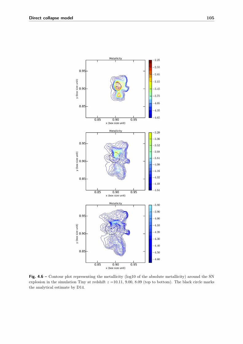
Direct collapse model 105

Fig. 4.6 – Contour plot representing the metallicity (log10 of the absolute metallicity) around the SNexplosion in the simulation Tiny at redshift z =10.11, 9.00, 8.09 (top to bottom). The black circle marksthe analytical estimate by D14.

106 4.8 Conclusions

gas, all the efficient coolants, namely metals and molecular hydrogen, must be absent. Thedestruction and the prevention of molecular hydrogen can be done by a strong photo-dissociatingradiation coming from nearby star-forming galaxies. A large inflow rate of gas at the center ofthe halo, higher than 0.1 M/yr for at least one free-fall time, is required in order to form asupermassive star-like object.

The feasibility of the direct collapse mechanism is difficult to investigate. Zoom-in simulationsinvestigate the collapse and the accretion properties (e.g., Latif et al., 2013a ; Regan, Johansson& Wise, 2014 ; Hartwig et al., 2015), but use an artificial radiation intensity. Larger scalesimulations, such as Chunky or FiBY (the simulation used for A14), instead model the spatiallyvarying radiation intensity but are not able to follow the collapse, the accretion rate in the innerpart of the halo, neither to model individually the radiation coming from each star. Employingsmall hydrodynamical simulation boxes has the advantage of resolving in detail different aspectsof the problem (chemistry, mini-halos, early metal-enrichment, for example), but fails to presenta large diversity of cosmological regions, biasing the derived number density of DC regions.

In this chapter, we use three sizes of simulation box, from a small box of 1 cMpc side length,a medium box of 10 cMpc with a set of two simulations, and a large simulation box of 142 cMpc.We model the radiation intensity coming from nearby star-forming galaxies in a similar way asD14 and A14. Our attempt was to estimate the number density of regions eligible to host aDCBH, based on the absence of efficient coolants criterion: a high enough radiation intensity todestroy molecular hydrogen and a low metallicity. The idea was not to capture all the physicalprocesses at the same time in the same simulation, but to have a larger picture of the directcollapse scenario by using, for the first time, a suite of large scale hydrodynamical simulations.Another aim was to see if some halos were illuminated by a sufficiently high radiation intensity(JLW,crit = 100, 300), more similar to what is obtained as critical value for collapse in 3D zoom-insimulations.

We investigated the impact of SN feedback. We use either a weaker thermal feedback ora stronger delayed cooling feedback. Star formation is lower (by one order of magnitude) inthe simulation with delayed cooling SN feedback, and more in line with the predictions of halooccupation distribution (Habouzit, Volonteri & Dubois, 2016). A weak SN feedback allows formore young stars, but also, consequently, for an earlier metal pollution. Using our DCBH findercode (with tff as in D14 and JLW,crit = 30), we do not find any DCBH regions in the simulationChunky with the delayed cooling feedback, however we do find 3 regions for the thermal SNfeedback. The absence of a strong radiation field, caused by the lower star formation rate,therefore, appears to be more important than metal pollution. Besides, in these 10 cMpc sidebox, we do not find any halo illuminated by a radiation intensity higher than 162.71 in JLWunits, down to z = 7.33, so no DCBH can form if JLW,crit 100. For the delayed cooling SNfeedback, the maximum value of the radiation intensity is only JLW = 30.33.

The simulation Horizon-noAGN allows us to have a more global view of the direct collapsescenario. The simulation box is large enough to have some statistics (box side length of 142cMpc), at the price of a lower resolution, and it includes a relatively weak SN feedback. Thenumber density of DCBH regions in this simulation varies from 7×10−7 to 10−4 cMpc−3. We findsimilar results as D14, specifically for the two largest thresholds JLW,crit = 100 and JLW,crit = 300.However, the number density of BHs for the threshold JLW,crit = 30 for the Horizon-noAGNsimulation is smaller than what D14 and A14 obtained for the same threshold. We do notconsider a radiation background, and this can have an impact when considering low intensitythresholds such as JLW,crit = 30. Horizon-noAGN also allows us to investigate whether the DCscenario can explain the presence of BHs in massive galaxies at z = 6, considered as proxies for

Direct collapse model 107

the hosts of quasars. We find that 30% of the halos more massive than 1011 M at z = 5.8, haveat least one progenitor eligible to form a DCBH for JLW,crit = 30. This probability, however,drops abruptly below 1-10% when considering higher thresholds (JLW,crit = 100, 300) for theradiation intensity.

Several approaches have been used in the last few years to determine the number density ofdirect collapse regions, from post-processing of hydrodynamical simulations to semi-analyticalmethods. These approaches derive number density which differ by several orders of magnitude(from 10−1 to 10−9 Mpc−3). We perform a comparison between some of these approaches,specifically with A14 and D14, in order to understand this discrepancy. We find differences inthe probability for halos to be star-forming and metal-free, for the propagation of metals in thegas, and finally in the modeling of the radiation intensity itself, which in some cases compensateto produce similar results in the number density, despite the very different single assumptions.

In summary, we find that if DC requires JLW,crit = 300, and a halo must be illuminated bysuch intense field for its full collapse, the number of DCBHs may be sufficient to explain thenumber of high-z quasars, based on Horizon-noAGN, but not the presence of BHs in normalgalaxies. If instead either JLW,crit ∼ 30 or a halo must be illuminated only during the collapseof the central region, then DCBHs may be common also in normal galaxies, provided that SNfeedback is not very strong.

4.9 Perspectives: Applications of hybrid SAMs

Hybrid SAMs as the bridge between SAMs and zoom-in cosmological hydrodynamical sim-ulations

As we have said in the introduction of this chapter, hybrid semi-analytical models are thebridge between pure SAMs and cosmological hydrodynamical zoom-in simulations of single halos.Zoom-in simulations reach high spatial resolution, and are able to follow the gas collapse to highdensities. However, they are lacking of validation for the occurrence of a zoom-in physical setup. Hybrid SAMs are therefore needed to provide a set of reasonable parameters, for instance,metallicity, background radiation intensity. They are also crucial to place the zoom-in simulationsin a more global context, and to provide an idea of the occurrence of the processes studied inzoom-in simulations. In the following, we give an example of an applications of hydrodynamicalsimulations: the fraction of metal enriched halos (Latif et al., 2016).

In Latif et al. (2016), we have studied the impact of dust and metal line cooling in massiveprimordial halos (Mh > 107 M) illuminated by a strong radiation intensity, and polluted bytrace amounts of metals and dust. The importance of dust in gas fragmentation has been shownby Schneider et al. (2003) ; Omukai et al. (2005) ; Omukai, Schneider & Haiman (2008), thepresence of dust will boost the cooling of the gas, which favors the fragmentation of the gas.Formation of H2 on dust grains also boosts the cooling of the gas (Omukai, 2001 ; Cazaux &Spaans, 2009 ; Latif, Schleicher & Spaans, 2012). We have performed 3D zoom-in cosmologicalsimulations of two halos with the code Enzo, which includes here cooling and heating from dustgrains. The isothermal collapse of the gas is possible, even in the presence of trace metals anddust, until reaching densities of 10−16 g cm−3, at which dust cooling becomes effective. We findthat dust cooling is more efficient for high metallicities. Regarding the inflow rate, which is ofparamount importance in the DC BH formation model, we find that inflow rate of 0.1 M/yr isfeasible for Z 6 10−5 Z, and decreases for higher metallicities. Compared to metal-free halos,

108 4.9 Perspectives: Applications of hybrid SAMs

Fig. 4.7 – Fraction of metal below a given mean halo metallicity, Z < 10−4 Z in blue, Z < 10−5 Z ingreen, Z < 10−5 Z in red, and finally Z = 0 in black. Published in (Latif et al., 2016).

by which factor the fraction of DC eligible halos increase for metallicity of Z 6 10−5 Z?To answer this question and to give a large scale perspective to this work, we have run acosmological hydrodynamical simulation Chubby, which is similar to the simulation Chunky,but with a better spatial and dark matter resolution. The box size is (10 cMpc)3, and allowsus to have some statistics. Chubby is very similar to Chunky (described above) in terms ofthe cosmology used, star formation recipe, AGN feedback, SN feedback. We use the delayedcooling SN feedback implementation, with the parameter MSN = 3.2× 103 M, σen = 54 km s−1,tdiss = 0.7 Myr. The box side is again 10 cMpc−3. We run the simulation from z = 200 down toz = 6, we stop at this redshift because sufficient for the study we described, and also becausesuch a high resolution simulation is very time consuming. The spatial resolution is ∆x = 10 pc,and he mass resolution MDM,res = 2× 105 M.With the simulation Chubby, we estimate the fraction of halos that are metal-polluted withZ < 10−4 Z (Latif et al., 2016). With HaloMaker, we identify all the halos in the massrange 2 × 107 − 108 M that at least contain 100 dark matter particles. Fig. 4.7 show thefraction of metal below a given mean halo metallicity, Z < 10−4 Z in blue, Z < 10−5 Z ingreen, Z < 10−5 Z in red, and finally Z = 0 in black. The number of halos under a given meanmetallicity decreases with decreasing redshift. The fraction of halos polluted with Z 6 10−5 Zis ∼ 1.5 higher than the fraction of metal-free halos. Therefore, if the DC model is feasible forZ 6 10−5 Z, the fraction of DC candidate halos is increased by 1.5 compared to metal-free halos.

Hybrid SAMs as template for full self-consistent cosmological hydrodynamical simulations

Hybrid SAMs offer us the advantage of following in time different crucial quantities for the DCBH formation model, such as metal-enrichment of the gas, stellar formation, spatial distributionof halos. This is crucial to determine which halos are eligible for the formation of DCBHs.Unfortunately, following in time the growth of these DCBH is still limited by our inability of

Direct collapse model 109

forming DCBHs self-consistently on-the-fly in hydrodynamical simulations. Based on the workwe have described in this chapter, we would like to implement in the code Ramses the DCformation scenario.The implementation will be based on the metallicity of the local environment of the future BHs,the stellar mass and the distance of nearby star-forming regions, a collapsing time or free-falltime (during which the radiation coming from the star-forming regions has to be higher thana given threshold.) All the regions matching these criteria, will be seeded with a sink particleand flagged as DCBH. Doing it on-the-fly will allow us to self-consistently make predictions onthe observational diagnostics for BH formation for the different BH formation models, namelythe light seed models presented in the previous chapter, and the DC heavy seed model: mass ofBH, BH-galaxy occupation fraction. Having all these BH formation scenarios implemented inthe same simulation code will allow us to study the impact of both the low-mass and high-massseeds, through AGN feedback, on their host galaxies, for example.This project will require a larger simulation box size. As we have seen in this chapter, in asimulation box of 10 cMpc side length, only few, if any, DC candidate halos are found, this projectwill therefore require a larger simulation box size, with a spatial and dark matter resolutionscomparable to those of the simulation Chubby.

110 4.9 Perspectives: Applications of hybrid SAMs

Chapter 5Black hole formation and growth with primordialnon-Gaussianities

The chapter treats different topics in the fields of galaxy formation and evolution, reionizationhistory, and the formation and growth of supermassive black holes. How do the prescription of thecosmological model affect the evolution of the Universe and the formation of large scale structures,and massive objects? Planck mission recently provided strong limits on non-Gaussianity on scalesof clusters, but there is still room for considerable non-Gaussianity on galactic scales. We havetested the effect of local non-Gaussianity by running five cosmological N -body simulations downto z = 6.5. For these simulations, we adopt the same initial phases, and either Gaussian or scale-dependent non-Gaussian primordial fluctuations, all consistent with the constraints set by Planckon cluster scales. We particularly focus on the impact of non-Gaussianities on high-redshift darkmatter halos, and galaxy population, on the reionization history of the Universe, and finally onsupermassive BH formation and evolution over cosmic time. The main result of the introductionof primordial non-Gaussian fluctuations is the assembly of more low-mass dark matter halos.The galaxy mass function is also enhanced by a maximum of 0.3 dex at the low-mass end. Thisleads to an increase of the number of sources providing ionizing photons, resulting in an earlyreionization period. These more numerous low-mass galaxies, are potential extra sites for BHformation, we investigate the two most common BH formation models, the PopIII remnants andthe direct collapse models.

This chapter is adapted from its corresponding publications:

• Testing primordial non-Gaussinities on galactic scales at high-redshift,Mélanie Habouzit, Takahiro Nishimichi, Sébastien Peirani, Yohan Dubois, Gary Mamon,Joseph Silk and Jacopo Chevallard,MNRAS, 2014, vol 445, pages L129-L133, arXiv:1407.8192

• Effect of primordial non-Gaussianities on the far-UV luminosity function of high-redshift,Jacopo Chevallard, Joseph Silk, Takahiro Nishimich, Mélanie Habouzit, Gary Mamon,Sébastien Peirani,MNRAS, 2015, vol 446, pages 3235-3252, arXiv:1410.7768

• Black hole formation and growth with non-Gaussian primordial density perturbations,Mélanie Habouzit, Marta Volonteri, Muhammad Latif, Takahiro Nishimichi, SébastienPeirani, Yohan Dubois, Gary Mamon, Joseph Silk and Jacopo Chevallard,MNRAS, 2016, vol 456, pages 1901-1912, arXiv:1507.05971

111

112 5.1 Introduction on primordial non-Gaussianities

Contents5.1 Introduction on primordial non-Gaussianities . . . . . . . . . . . . . 112

5.1.1 Primordial bispectrum . . . . . . . . . . . . . . . . . . . . . . . . . . . . 1135.1.2 Introduction of fNL parameter . . . . . . . . . . . . . . . . . . . . . . . 1145.1.3 Observational constraints, room for non-Gaussianities at small scales . . 1165.1.4 Previous work, and the idea of running non-Gaussianities . . . . . . . . 116

5.2 Halo and galaxy mass functions . . . . . . . . . . . . . . . . . . . . . . 1185.2.1 Numerical methods: from non-Gaussian N -body simulations to galaxy

formation model . . . . . . . . . . . . . . . . . . . . . . . . . . . . . . . 1185.2.2 Predicted halo mass functions from theory . . . . . . . . . . . . . . . . . 1205.2.3 Results on halo and galaxy mass function . . . . . . . . . . . . . . . . . 1215.2.4 Conclusions . . . . . . . . . . . . . . . . . . . . . . . . . . . . . . . . . . 123

5.3 Reionization history of the Universe . . . . . . . . . . . . . . . . . . . 1245.3.1 Far-UV luminosity function and reionization models . . . . . . . . . . . 1245.3.2 Fraction of ionized volume of the Universe . . . . . . . . . . . . . . . . . 1255.3.3 Electron Thomson scattering optical depth . . . . . . . . . . . . . . . . 1265.3.4 Conclusions . . . . . . . . . . . . . . . . . . . . . . . . . . . . . . . . . . 127

5.4 BH formation and growth with primordial non-Gaussianities . . . . 1285.4.1 BHs formed through direct collapse . . . . . . . . . . . . . . . . . . . . 1295.4.2 BHs formed from the remnants of the first generation of stars. . . . . . 1375.4.3 BHs in the most massive halos at z = 6.5 . . . . . . . . . . . . . . . . . 1385.4.4 Conclusions . . . . . . . . . . . . . . . . . . . . . . . . . . . . . . . . . . 141

5.1 Introduction on primordial non-Gaussianities

The cosmological principle predicts an uniform and isotropic distribution of matter in the Universe.In order to form large scale structures, one needs to introduce perturbations in the history ofthe Universe. The Hot Big Bang theory has no explanation for the non-uniform and isotropicdistribution of matter, and it is one of the so-called problems of this theory (the two others beingthe flatness problem and the horizon problem). The standard description of the Universe, drivenby the general theory of relativity, is expected to break down when the Universe is so dense thatquantum effects may be more than important to consider. Inflation theory has been consideredto be a natural physical process solving the Hot Big Bang theory’s problems, since almost 40years ago. In addition to solving the Hot Big Bang problems, this accelerated period of ourUniverse allows the introduction of these quantum processes, which can produce the necessaryspectrum of primordial density seed perturbations, that gravitational instability accentuates toproduce the large structures we observe today, namely dark matter halos, clusters and galaxies.

Inflation was also able to explain the CMB temperature anisotropies, that is why inflationarytheory has became very appealing and studied over the years. The temperature anisotropies ofthe CMB, measured by COBE (Smoot et al., 1992 ; Bennett et al., 1996 ; Gorski et al., 1996),WMAP (Spergel et al., 2003 ; Komatsu et al., 2003) and Planck (Planck Collaboration et al.,2011, 2015b,a) missions, are relics of density perturbations in the cosmic fluid at the timeof last scattering (through the Sachs-Wolfe effect). Primordial perturbations described by aGaussian distribution is supported, on large scales, by the measurements of these temperature

Black hole formation and growth with primordial non-Gaussianities 113

anisotropies of the CMB, since the first detection of anisotropies by COBE in 2001. Planck’sresults (Planck Collaboration et al., 2014, 2015b) have made incomparable progress in theaccuracy of the estimated cosmological parameters and on our knowledge of the beginning of theUniverse. The Planck mission has, however, focused on large structures, considering primordialdensity perturbations on the scale of clusters. Mapping in detail the CMB on the full sky,it has provided very strong constraints on the local non-Gaussian parameter fNL = 2.7 ± 5.8(Planck Collaboration et al., 2013b), which describes the deviation to a Gaussian distribution ofprimordial density fluctuations, and will be explained in more detail in the next section. However,as predicted by some inflationary models, non-Gaussianities on smaller scales, beyond the reachof CMB measurements, are still conceivable.

As nicely discussed in Bartolo et al. (2004), the question is not to probe that CMB isconsistent with Gaussianities, but rather to ask “How Gaussian is it?”. Investigating and testingthe Gaussianity of the CMB is a very difficult task, and this is due to the fact that non-Gaussianfluctuations have infinite degrees of freedom (in other words, there is an infinite number of waysof being non-Gaussian). The observed signal of the CMB is the result of a summation of differenteffects arising from different sources, that all contribute to the observed signal. They can comefrom non-Gaussianities in the primordial curvature perturbation produced in the very earlyuniverse by inflation (the purpose of this work), but also from non-Gaussianity arising afterrecombination as lensing, or generated by galactic and extra galactic sources. Extracting theinformation of primordial non-Gaussianity is challenging for these reasons. In this chapter, wewill focus only on primordial non-Gaussianities, and investigate their impact on the Universeevolution with cosmological simulations. In the following, we start with a short introduction onprimordial non-Gaussianities. We then describe the consequences of non-Gaussianities in theassembly of large structures, both dark matter halos and galaxies, on the reionization history,and finally on black hole formation and evolution.

5.1.1 Primordial bispectrum

Probes of inflation theory come from properties of fluctuations. Standard models of inflationpredicts a flat Universe perturbed by nearly Gaussian and scale invariant primordial fluctuations(Gangui et al., 1994 ; Acquaviva et al., 2003 ; Maldacena, 2003). Primordial non-Gaussianitiesare therefore an important test of how physics shaped the universe at early times, at energiestoo high to be probed by laboratory experiments. Non-Gaussianities are a promising way toinvestigate inflation, and specifically the interactions of the field generating inflation.To define the standard inflationary observables, we characterize the scalar degree of freedomin the primordial density perturbations using the curvature perturbation on a uniform densityhypersurface ξ (gauge-invariant, and can be related to the field fluctuations during inflation andthe temperature fluctuations in the CMB).Power spectrum Pξ is defined by the two-point correlation function and described the statisticalproperties of the primordial density perturbations:

< ξk1ξk2 >= (2π)3Pξ(k1)δ(3)(k1 + k2), (5.1)

ki the comoving wavevectors, δ(3) the three dimensional Dirac delta function, ξk the Fouriertransform of ξ. If ξ is a purely Gaussian field then the two-point correlation function completelydefines the statistics of the field. To acceed any departure from a Gaussian field, which isnot encoded in the power spectrum Pξ, one requires to measure higher order of correlations.Therefore for a non-Gaussian field, higher-order correlations are needed, with the three-point

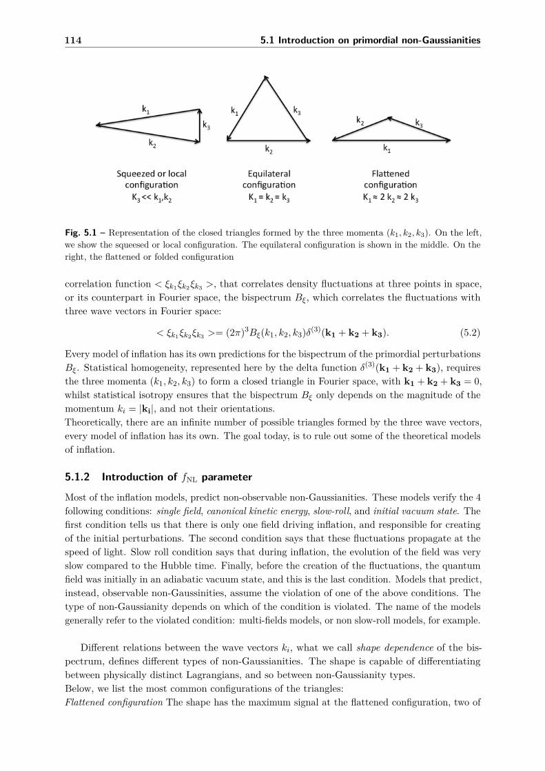
114 5.1 Introduction on primordial non-Gaussianities

Fig. 5.1 – Representation of the closed triangles formed by the three momenta (k1, k2, k3). On the left,we show the squeesed or local configuration. The equilateral configuration is shown in the middle. On theright, the flattened or folded configuration

correlation function < ξk1ξk2ξk3 >, that correlates density fluctuations at three points in space,or its counterpart in Fourier space, the bispectrum Bξ, which correlates the fluctuations withthree wave vectors in Fourier space:

< ξk1ξk2ξk3 >= (2π)3Bξ(k1, k2, k3)δ(3)(k1 + k2 + k3). (5.2)

Every model of inflation has its own predictions for the bispectrum of the primordial perturbationsBξ. Statistical homogeneity, represented here by the delta function δ(3)(k1 + k2 + k3), requiresthe three momenta (k1, k2, k3) to form a closed triangle in Fourier space, with k1 + k2 + k3 = 0,whilst statistical isotropy ensures that the bispectrum Bξ only depends on the magnitude of themomentum ki = |ki|, and not their orientations.Theoretically, there are an infinite number of possible triangles formed by the three wave vectors,every model of inflation has its own. The goal today, is to rule out some of the theoretical modelsof inflation.

5.1.2 Introduction of fNL parameter

Most of the inflation models, predict non-observable non-Gaussianities. These models verify the 4following conditions: single field, canonical kinetic energy, slow-roll, and initial vacuum state. Thefirst condition tells us that there is only one field driving inflation, and responsible for creatingof the initial perturbations. The second condition says that these fluctuations propagate at thespeed of light. Slow roll condition says that during inflation, the evolution of the field was veryslow compared to the Hubble time. Finally, before the creation of the fluctuations, the quantumfield was initially in an adiabatic vacuum state, and this is the last condition. Models that predict,instead, observable non-Gaussinities, assume the violation of one of the above conditions. Thetype of non-Gaussianity depends on which of the condition is violated. The name of the modelsgenerally refer to the violated condition: multi-fields models, or non slow-roll models, for example.

Different relations between the wave vectors ki, what we call shape dependence of the bis-pectrum, defines different types of non-Gaussianities. The shape is capable of differentiatingbetween physically distinct Lagrangians, and so between non-Gaussianity types.Below, we list the most common configurations of the triangles:Flattened configuration The shape has the maximum signal at the flattened configuration, two of

Black hole formation and growth with primordial non-Gaussianities 115

the three wavenumbers are equal and twice the value of the third vector, k1 ≈ 2 k2 ≈ 2 k3 (seelast figure in Fig. 5.1). This configuration is produced by non-vacuum initial condition.Equilateral configuration This configuration is characterized by k1 = k2 = k3 (representation inthe middle of Fig. 5.1). This shape can be produced by non canonical kinetic terms of quantumfields.Squeezed or local configuration This is produced by considering multiple fields inflation models.The most studied primordial bispectrum is the local-type model, also called the squeezed configu-ration. Interactions that are local in real space (that is why we call them local non-Gaussianities)therefore maximize the bispectrum in the squeezed configuration (cf the left panel in Fig. 5.1),when two of the wavenumbers are much greater than the third one k3 << k1, k2 (Gangui et al.,1994).

They are two distinct features of the bispectrum that help us probe the inflationary action.The first one is its overall amplitude, which is often parametrized (Komatsu & Spergel, 2001)by the non-linearity parameter fNL (for a given model of Bξ). fNL measures the level of thenon-Gaussianity signature.

We can express the bispectrum as a function of the fNL parameter, and a function T (k1k2, k3)which capture its dependence on the triangle configurations:

Bξ ≡ fNL T (k1k2, k3). (5.3)

The magnitude of the non-Gaussianity of local configuration can be parameterized (Komatsu& Spergel, 2001) by the parameter fNL, describing the quadratic coupling of the primordialperturbations. The gravitational potential can be split in two components, a Gaussian fieldgiven the usual perturbation results, described by ζG(x), and a small local non-Gaussian term,described by ζG(x) = fNL

(ζ2

G(x)−⟨ζ2

G(x)⟩)

. The resulting curvature perturbations ζ(x) at agiven position x, can therefore be expressed by:

ζ(x) = ζG(x) + 35fNL

(ζ2

G(x)−⟨ζ2

G(x)⟩), (5.4)

where ζG is a Gaussian random field at the same position. In other words, we parametrizednon-Gaussianity as a non-linear correction to a Gaussian perturbation ζG. The factor 3/5 isconventional and comes from the fact that initially the equation was expressed in terms of the New-tonian potential Φ(x), which is related to ζ by the factor 3/5 during the matter-dominated period.

We need to keep in mind that we have confirmed over the years that inflation has producedprimordial fluctuations, however we still have not identified the mechanisms by which thesefluctuations are generated. Of course, several scenarios have been proposed. The slow-rollscenario is the standard scenario (fluctuations of the inflation field when it slowly rolls downalong its potential, produce the cosmological density fluctuations). This scenario predict fNL ∼ ε,where ε 1 is the slow roll parameter, which is independent of scale (Maldacena, 2003). Wecan also cite the curvaton scenario (Mollerach, 1990 ; Enqvist & Sloth, 2002 ; Lyth & Wands,2002), but also the inhomogeneous reheating one (Dvali, Gruzinov & Zaldarriaga, 2004), or theghost inflationary scenario (Arkani-Hamed et al., 2004).

116 5.1 Introduction on primordial non-Gaussianities

5.1.3 Observational constraints, room for non-Gaussianities at small scales

The primordial density fluctuations evolve with time, and lead to the collapse of dark matterparticles, and baryons. A non-Gaussian initial spectrum of density perturbations will then affectthe distribution of baryonic structures. The large scale structures of the Universe therefore arethe results of the non-linear evolution due to gravitational instability of some initial densityperturbations, which are also responsible for the CMB anisotropies. The CMB provides us amap of the density perturbations at the time of decoupling, the earliest information we haveabout our Universe. Studying CMB anisotropies give us amazing insight of non-Gaussianities.

In the field of cosmological perturbations, measuring the parameter fNL has been one ofthe primary goals of several spatial missions. The first attempt was with the satellite COsmicBackground Explorer (COBE), which was launched on the 18th of November 1989 1. In 2001,the data of the Differential Microwave Radiometer instrument DMR allowed a first estimate of|fNL| < 1500 (68%), via the angular bispectrum, which is the harmonic counterpart of the three-point correlation function. While this limit has ben obtained for large-scale non-Gaussianities,with the MAXIMA data, a limit at small scales has also been determined, |fNL| < 950 (68%).Despite an interesting range of methods to compute a value for the fNL parameter, and differentfinal values, the COBE satellite only gave us a weak constrain.

Wilkinson Microwave Anisotropy Probe (WMAP) satellite has been launched on June 30,2001. The first results were released in 2003, and further results were released in 2005, 2007,2009 and 2011. The constraints on the parameter fNL have been highly debated, because ofthe scatter obtained in the constraints by different teams, but with the same set of data. Weonly cite here the estimate of Smith, Senatore & Zaldarriaga (2009), with −4 < fNL < 80 (95%,WMAP-5years).

The Planck satellite was launched in 2009, it has provided a much stronger constraint onthe local non-Gaussianity parameter, fNL = 2.7± 5.8 (Planck Collaboration et al., 2013b), thandid the previous CMB missions. This new constraint on fNL on large scales does not excludenon-Gaussianity on smaller scales, on galactic scales.

5.1.4 Previous work, and the idea of running non-Gaussianities

By appealing to the theory of Press & Schechter (1974) it is straightforward to show that positivelyskewed (fNL > 0) primordial density fluctuations increase the halo mass function (HMF) at largemasses with respect to that arising from Gaussian initial conditions (e.g. Matarrese, Verde &Jimenez, 2000). This effect has also been verified with cosmological N -body simulations (Kang,Norberg & Silk, 2007 ; Grossi et al., 2007 ; Pillepich, Porciani & Hahn, 2010). Simulations withnon-Gaussian initial conditions (nGICs) have been used to probe the halo mass function (Kang,Norberg & Silk, 2007; Grossi et al., 2007; Pillepich, Porciani, & Hahn, 2010), the scale-dependenthalo bias (Dalal et al., 2008; Desjacques, Seljak & Iliev, 2009; Grossi et al., 2009) and bispectrum(Nishimichi et al., 2010; Sefusatti, Crocce, & Desjacques, 2010), weak lensing statistics (Paceet al., 2011; Shirasaki, Yoshida, Hamana, & Nishimichi, 2012), the pairwise velocity distributionfunction (Lam, Nishimichi, & Yoshida, 2011). Hydrodynamical cosmological simulations havebeen performed with nGICs to study the baryon history (Maio & Iannuzzi, 2011), the gasdistribution (Maio, 2011), the gas density profiles (Maio & Khochfar, 2012) and SZ maps (Pace& Maio, 2014).

1That was few months after my birth date, meaning that I am as old as COBE satellite

Black hole formation and growth with primordial non-Gaussianities 117

Fig. 5.2 – Example of running models for non-Gaussianity parameter fNL in solid or dashed lines, byLoVerde et al. (2008). Range of scales probed by different observables are also shown in green region forCMB, blue for galaxy bispectrum, and yellow for clusters.

These studies have all used a scale-independent value of fNL. However, the new constraint onfNL on large scales does not exclude non-Gaussianity on smaller scales, namely on galactic scales.Indeed, the non-Gaussianity might depend on scale, as predicted, e.g., in several inflation modelswith a variable speed of sound, such as the string-based Dirac-Born-Infeld models (Silverstein &Tong, 2004 ; Alishahiha, Silverstein & Tong, 2004 ; Chen, 2005).An extra-dependence of scale k, can be described as a running prescription for the parameterfNL, that we can therefore expressed as:

fNL(k) = fNL,0

(k

k0

)α, (5.5)

where k0 is a pivot scale.It is thus possible that significant non-Gaussianity can lurk on the comoving scales of galaxies

without being detected by the Planck CMB mission, whose angular resolution effectively limits itto the scales of clusters of galaxies. A blue spectrum of running non-Gaussianity might enhancelow masses instead, if the spectrum is blue enough, i.e. if α = d ln fNL/d ln k is large enough. Theeffects of scale-dependent non-Gaussianity on the HMF (cluster counts) and on reionization wereanalytically predicted by LoVerde et al. (2008) and Crociani et al. (2009), respectively. LoVerdeet al. (2008) study the possibility of constraining the running parameter α with a coalition ofdifferent methods, CMB measurements, but also the measurements of cluster abundance. Therange of scales probed by the different observables are shown in Fig.5.2, in green the regionexcluded by CMB measurements, in blue the scales probed by the galaxy spectrum, and finallyin yellow the scales probed by cluster surveys. The scale dependence α of the parameter fNL,implies a different level of non-Gaussianities at different scales k. LoVerde et al. (2008) consideran equilateral model here, however the principle remains the same as what we investigate in thischapter with local non-Gaussianity on galactic scales.

Because small scales are still poorly constrained at high redshifts (z > 6), cosmological

118 5.2 Halo and galaxy mass functions

Tab. 5.1 – Characteristics of fNL models (eq. [5.6])

Model G NG1 NG2 NG3 NG4fNL,0 0 82 1000 7357 10000α – 1/2 4/3 2 4/3

simulations are key for predicting whether non-Gaussianities have an impact on galactic scales.Only one team has run nG simulations with an explicit scale-dependence adjustable by a freeparameter (Shandera, Dalal & Huterer, 2011), focusing on halo clustering in the the local Universe.In the following, we describe the method that we use to investigate non-Gaussianity, namely thesimulation set-up and the various models of scale-dependent fNL parameter.

5.2 Effects of non-Gaussianities on the Universe structure formation:halo and galaxy mass functions

5.2.1 Numerical methods: from non-Gaussian N-body simulations to galaxy for-mation model

Initial conditions: prescription for fNL and N-body simulations

We employed a simple model that allows a significant amount of non-Gaussianity on smallscales, relevant for early structure formation, while keeping such effects small on large scales tomeet the strong constraints obtained by the Planck CMB mission (Planck Collaboration et al.,2013b). We model the scale-dependent non-linearity parameter fNL as:

fNL(k) = fNL,0

(k

k0

)α(5.6)

We explored four different non-Gaussian (nG) models by varying the normalization fNL,0 andthe slope α = d ln fNL/d ln k, in such a way that the non-Gaussianity is significant on galacticscales, yet small enough to meet the current constraints from Planck (Planck Collaboration et al.,2013b). Table 5.1 (normalization and slope for k0 = 100h/Mpc) lists our adopted models, whileFig. 5.3 displays these models with current constraints from CMB experiments. We restrictedourselves to positively skewed primordial density fluctuations, i.e. fNL > 0, hence fNL,0 > 0.

We modified the initial condition generator originally developed by Nishimichi et al. (2009),based on second-order Lagrangian perturbation theory (e.g., Scoccimarro, 1998 ; Crocce, Pueblas& Scoccimarro, 2006), parallelized by Valageas & Nishimichi (2011) and with local-type non-Gaussianities implemented by Nishimichi (2012). We followed Becker, Huterer & Kadota (2011)and realized the generalized local ansatz of equation (5.4) by taking a convolution of the curvaturesquared and the k-dependent fNL kernel in Fourier space. We used the public Boltzmann code,camb (Lewis, Challinor & Lasenby, 2000) to compute the transfer function and multiply it tothe curvature perturbations to have the linear density fluctuations.

N-body simulations and halo catalog

Black hole formation and growth with primordial non-Gaussianities 119

Fig. 5.3 – Models (lines) for the scale-dependent NG parameter f localNL . The orange shaded region represents

the allowed values from WMAP, within 1σ, of the f localNL (k) according to Becker & Huterer (2012). The

magenta shaded region shows the Planck constraint (Planck Collaboration et al., 2013b). The right edgeof the box corresponds to a scale of 2π/k ' 30 kpc, i.e. the scales of galaxies are to the right of the rightedge of the box.

We have performed five cosmological simulations with Gadget-2 (Springel, 2005) for a ΛCDMuniverse using Planck parameters (Planck Collaboration et al., 2013a), namely ΩM = 0.307,ΩΛ = 0.693, h = 0.678 and σ8 = 0.829. Each simulation was performed in a periodic box of side50h−1 Mpc with 10243 dark matter particles (e.g. with mass resolution of ∼ 9.9× 106 h−1 M).One simulation (hereafter, ‘G’) started with Gaussian ICs, while the other four (hereafter, ‘NG’)began with nGICs (eqs. [5.4] and [5.6], with parameters in Table 5.1), with the same initial phases.The simulations started at z = 200 and ended at z = 6.5. In each case, the Plummer-equivalentforce softening was set to 5% of the mean inter-particle distance (2.44h−1 kpc in comoving units).

For each snapshot (taken every ∼ 40 Myr), catalogues of halos were prepared using Adapta-HOP (Aubert, Pichon, & Colombi, 2004), which employs an SPH-like kernel to compute densitiesat the location of each particle and partitions the ensemble of particles into (sub)halos based onsaddle points in the density field. Only halos or subhalos containing at least 20 particles (e.g.2.9× 108M) were retained. We then studied the individual evolution of (sub)halos, by buildinghalo merger trees using TreeMaker (Tweed et al., 2009), which allowed us to accurately derivethe mass evolution of each dark matter (sub)halo. This was the basis to compute the evolutionof galaxy stellar masses, as we shall see in Sect. 5.2.3.

Galaxy formation and evolution model

Galaxy stellar masses are “painted” on the halos and subhalos using the Behroozi, Wechsler,& Conroy (2013) model that provides the galaxy mass m as a function of halo mass M andredshift z. We could have adopted a physical model, such as Cattaneo et al. (2011). We alsoconsidered using the empirical model of Mutch, Croton, & Poole (2013). The former model isonly constrained at z = 0, while the latter extends to z = 4, which is still insufficient for ourpurposes. We have thus preferred to adopt the empirical model of Behroozi, Wechsler & Conroy,whose parameters were fit to the galaxy stellar mass functions, specific star formation rates and

120 5.2 Halo and galaxy mass functions

Fig. 5.4 – Analytical predictions of the nG correction to the halo mass function, for different power valuesof fNL. We plot the ratio of the halo mass function with non-Gaussian and Gaussian initial conditions atz = 10 (left) and z = 7 (right), for different running fNL(k) passing through the pivot point of the first 3models of Table 5.1 (see Fig. 5.3).

cosmic star formation rate, from z = 0 to z = 8. In particular, the Behroozi, Wechsler & Conroymodel is the only empirical model of galaxy mass vs. halo mass and redshift that extends upto the redshift when reionization is thought to occur. A weakness of our approach is that, forlack of a better simple model, we assume that the Behroozi, Wechsler & Conroy model can beextrapolated beyond z = 8 to z = 17.

The Behroozi, Wechsler & Conroy model was calibrated with HMFs derived from cosmologicalsimulations with Gaussian ICs. One could argue that their model cannot be applied to simulationswith nGICs, without appropriate corrections. Alternatively, one could adopt the Behroozi,Wechsler & Conroy model as a basis to which we can compare the effects of Gaussian vsnon-Gaussian ICs, and this is what we do here.

However, we slightly modify the Behroozi, Wechsler & Conroy model, by preventing galaxymasses from decreasing in time. For quiescent (sub)halos, we simply apply m(M, z), while formerging (sub)halos, we compare the galaxy mass m(M, z) to the sum over all its progenitors (inthe previous timestep). If the galaxy mass from the model is higher than the sum of progenitormasses, we apply m(M, z); if the galaxy mass is smaller, the new galaxy mass is the sum over allits progenitors.

5.2.2 Predicted halo mass functions from theory

Before discussing the results of our numerical simulations, it is worth presenting analyticalpredictions to gain insight into the potential consequences of scale-dependent non-Gaussianitieson early structure formation. We here adopt a simple model and discuss the effects on the HMF.

We follow the Press-Schechter formalism (Press & Schechter, 1974) for this calculation.Namely, we work with the linear density field, δM , smoothed with a spherical top hat windowthat encompasses a mass M and linearly extrapolated to z = 0, and consider that the one-pointcumulants of this field uniquely determine the HMF. Assuming that the nG correction is small,we apply the Edgeworth expansion to the one-point density probability distribution function(LoVerde et al., 2008). Up to the skewness order, the non-Gaussian to Gaussian ratio of the

Black hole formation and growth with primordial non-Gaussianities 121

HMF is given by

dnnG/dMdnG/dM (M, z) = 1 + 1

6C(3)M H3(ν) + 1

6dC(3)

M

d ln σMH2(ν)ν

, (5.7)

where σ2(M) =⟨δ2M

⟩is the variance of the density fluctuations δM , C(3)

M =⟨δ3M

⟩/σ3

M is ameasure of the skewness of δM , ν = δc(z)/σ(M) is the peak height, given δc(z) = 1.686/D+(z),the threshold density contrast for spherical collapse at redshift z, where D+(z) is the growthrate, and finally Hn is the Hermite polynomial.

In this model, all the nG correction comes from the skewness, which can be expressed by anintegral of the bispectrum:

〈δ3M 〉 =

∫ d3pd3q(2π)6 M(p)M(q)M(|p + q|)Bζ(p, q, |p + q|), (5.8)

whereM stands for the transfer function from the curvature to the density fluctuation smoothedby a mass scale M , and the bispectrum of the curvature ζ in the model (5.4) is given by

Bζ(k1, k2, k3) = 65 [fNL(k1)Pζ(k2)Pζ(k3) + (cyc. 2)] , (5.9)

where (cyc. 2) denotes two more terms that are obtained by cyclic permutation of the wavenumbersin the first term. The k dependence of fNL propagates to the mass dependence of skewnessthrough these equations, making the nG correction to the HMF rather non-trivial. Since wefocus on blue fNL (i.e., α > 0), we anticipate that the correction to the HMF gets larger at lowmasses.

Fig. 5.4 shows the analytical prediction (eq. [5.7]) at z = 10 (left) and z = 7 (right). Wehere adopt k0 = 5.11h/Mpc, fNL,0 = 18.5, which is the intersection of the models 1, 2 and 3(see Fig. 5.3), and vary the slope α as indicated in the figure legend. There are two noticeabletrends in Fig. 5.4. First, the dependence of the HMF ratio on M depends on the slope α: theboost from non-Gaussianity is an increasing function of M for α < 1, while a larger α results ina decreasing function of M . This high-mass enhancement of the HMF for small α is consistentwith LoVerde et al. (2008). Because of the ν-dependence in equation (5.7), rare objects receivemore non-Gaussian effect in these cases. When the k-dependence of fNL is blue enough, it is thelow-mass end of the HMF that is enhanced, so that the mass dependence in C(3)

M overwhelms thatof H3(ν). Second, the nG correction is more prominent at higher redshift. It is about a factor oftwo greater at z = 10 compared to z = 7. Although, not shown here, structure formation at lowredshift is almost unaffected with the models that we consider here (i.e., the change of dn/dM isless than 10% at z < 3 over the mass range shown in Fig. 5.4). Thus, early structure formationprovides us with a unique opportunity to constrain scale-dependent non-Gaussianity, given thevery tight Planck constraints on large scales.

5.2.3 Results on halo and galaxy mass function

The left-hand panels of Fig. 5.5 show the HMFs obtained from the five cosmological simulations.One sees (upper left panel of Fig. 5.5) that the effects of non-Gaussianity on the HMF areincreasingly important with increasing model number (see for example the upper left panel ofFig. 5.5).

Non-Gaussian models NG1 (α = 1/2) and NG2 (α = 4/3, low normalization) cause onlysmall (less than 0.1 dex) and insignificant enhancements of the HMF (top two left panels of

122 5.2 Halo and galaxy mass functions

Fig. 5.5 – Upper panels of boxes: halo (left) and galaxy stellar (right) mass functions (in Mpc−3dex−1)for different initial conditions: Gaussian models (dashed), and non-Gaussian models 1 to 4 (from top tobottom). Lower panels of boxes: residuals of the log mass function relative to that of the Gaussian run(the horizontal line shows equal non-Gaussian and Gaussian mass functions). The errors are Poisson.The different curves indicate different redshifts (decreasing upwards for the large boxes): z = 17 (black),z = 15 (blue), z = 13 (cyan), z = 10 (green), z = 8 (orange), and z = 7 (red).

Black hole formation and growth with primordial non-Gaussianities 123

Fig. 5.5) and SMF (top two right panels of Fig. 5.5). Non-Gaussian model NG3, with a verysteep slope (α = 2), produces significant enhancements (left panel in third row of Fig. 5.5) of upto 0.3 dex (z = 17) or 0.2 dex (z = 15), in the HMF at logM/M = 9. Finally, model NG4, witha slope 4/3 but a much higher normalization (10 times that of model NG2), produces very largeenhancements of the HMFs and SMFs at low masses and high redshifts: greater than 0.3 dexenhancements in the HMF arise for z ≥ 13 at all halo masses and z ≥ 10 for logM/M < 9.5.The corresponding SMF is also enhanced by over 0.3 dex for all galaxy masses at z ≥ 13 and atgalaxy masses log m/M ≤ 6.8 for z = 10.

5.2.4 Conclusions

We summarize the results presented in this first part of the chapter. In comparison with thepredictions from Gaussian ICs, simulations with ICs that are increasingly non-Gaussian atsmaller scales, yet consistent with the CMB constraints from Planck, can lead to small, buteventually detectable alterations to the halo and galaxy stellar mass functions. Since constantfNL > 0 enhances the HMF principally at large masses, one can think that low slopes ofα = d ln fNL/d ln k > 0 (keeping fNL > 0) should also enhance the high-end of the HMF, while ahigh enough slope should do the opposite and enhance the HMF at the low-mass end. At α = 2,the HMF is in fact enhanced, both at the high and low ends (left residual plot of third row ofFig. 5.5, although that of the high end is only marginally significant). However, for the shallowerslope (α = 4/3), the HMF is only enhanced at the low end. We find that our two strongestnon-Gaussian models (NG3, NG4) exhibit the largest differences, up to 0.2 dex for NG3 (α = 2),and greater than 0.3 dex (at z = 10) for NG4 (α = 4/3, fNL,0 = 10000). These effects of nGICson our simulated HMFs are close to the theoretical predictions, with some quantitative differences.

Unfortunately, it is difficult to measure the HMF with great accuracy, and considerably easierto measure the SMF. We used the state-of-the-art model of stellar mass versus halo mass andredshift of Behroozi, Wechsler & Conroy (2013) to produce galaxy masses on the (sub)halos ofour cosmological N -body simulations. We slightly altered the model to consider halo mergers andprevent galaxy masses from decreasing in time. Comparing the resultant galaxy mass functionsof our non-Gaussian models with that of our Gaussian model, we find similar behavior of theenhancements of the galaxy mass function with mass and redshift, i.e. 0.2 dex for NG3, and 0.3dex (at z = 10) for NG4.

The modification of the SMF by nGICs can have profound consequences. In particular, thereionization of the Universe by the first stars and galaxies will be affected, in a different waydepending on the slope α. Low mass galaxies are thought to be one of the most powerful sourcesof ionizing photons at high redshift (Robertson et al., 2013 ; Wise et al., 2014). Using a set ofcosmological simulations, we have seen that faint galaxies are the most affected by primordialnon-Gaussianities (see Models NG3 with α = 2 and NG4 with α = 4/3, but high normalization).Therefore primordial non-Gaussian perturbations can then strongly affect the thermal history ofthe intergalactic medium. Effects on the far-UV luminosity function and the reionization historyare discussed in the next section.

124 5.3 Reionization history of the Universe

5.3 Consequence of primordial non-Gaussianities on the reionizationhistory of the Universe

Using the same set of simulations, in Chevallard et al. (2015), we went further to address theimplications of scale-dependent non-Gaussianities on cosmic reionization. We only briefly describethe method of the study, the models that we have used and the main results.Reionization is thought to be mainly driven by UV radiation emitted by massive stars born in thefirst galaxies, and particularly by the low-mass galaxies, because hydrogen ionizing photons canescape more easily from low mass halos than high mass ones. The number of ionizing photonsemitted by early galaxies depends on their number density, i.e. on their far-UV galaxy luminosityfunction. We employed different reionization models (a fixed escape fraction fesc = 0.2, and twodifferent escape fractions varying with redshift, and different far-UV absolute magnitude limits)to investigate the ionization fraction of the Universe as a function of redshift. We quantify theimpact of the non-Gaussian primordial perturbations on the Universe reionization history, andon the optical depth of electrons to Thomson scattering.

5.3.1 Far-UV luminosity function and reionization models

Far-UV luminosity function

Instead of using the Behroozi model, this time we consider a modified semi-analytical galaxyformation model based on Mutch, Croton & Poole (2013) to compute the stellar mass assemblyin each dark matter halo. The stellar mass is linked to dark matter halo mass via two functions:

dM?

dt = Fgrowth × Fphys. (5.10)

The growth function Fgrowth gives the amount of baryons available to form stars,

Fgrowth = fbdMhalo

dt , (5.11)

where we take fb = 0.17 the baryon fraction of the Universe. Fphys described the fraction ofbaryons actually converted into stars. Instead of taking a log-normal function as in Mutch,Croton & Poole (2013), we use a log-Cauchy function, where the parameters are chosen to matchthe observed far-UV luminosity function of Bouwens et al. 2014 at z = 7.The Bruzual & Charlot (2003) stellar population synthesis code is used to compute the far-UV luminosity function for redshifts in the range 7 ≤ z ≤ 15. The effect of non-Gaussianitieson the far-UV luminosity function is very similar to the effect on the halo and galaxy mass function.

Reionization models

We consider a “standard” reionization model in order to compute the reionization of theUniverse. We can write the equation expressing the competition between processes of hydrogenionization by Lyman-continuum photons, and hydrogen recombination:

dQHIIdt = nion

〈nH〉− QHII

trec, (5.12)

where QHII is the volume filling fraction of ionized hydrogen. nion is the comoving productionrate of hydrogen ionizing photons within galaxies, and can be expressed as:

nion = fesc ξion ρUV. (5.13)

Black hole formation and growth with primordial non-Gaussianities 125

We assumed here that reionization is mainly driven by UV radiation emitted by massive stars inearly galaxies, therefore the comoving production rate of hydrogen depends on the UV galaxyluminosity function density, of the rate of Lyman-continuum photons per unit UV luminosity(computed at the wavelength 1500 Å). The UV luminosity density ρUV is computed by integratingthe Schechter fit to the UV luminosity function obtained for the different Gaussian and non-Gaussian simulations, and depends on the minimum galaxy luminosity. For the latter we alsouse two different values in the following, because it is an uncertain parameter as observations arecurrently only able to probe the bright end of the UV luminosity function at high redshift. fescis the escape fraction of these photons into the IGM, two different models of the escape fractionare assumed in this work, and detailed in the following. 〈nH〉 is the comoving average numberdensity of hydrogen atoms:

〈nH〉 = Xp Σb ρcmH

(5.14)

Finally, trec is the average recombination of time of hydrogen:

trec = (αB(T )neCHII)−1 (5.15)

with αB the hydrogen recombination coefficient, CHII the clumping factor which account forinhomogeneities in the density field, and ne the number density of free electrons, which canbe expressed as a function of redshift, 〈nH〉, and the fraction fe of free electrons per hydrogennucleus in the ionized IGM, via the relation ne = fe 〈nH〉 (1 + z)3.

The fraction of Lyman-continuum photons escaping their galaxies is one of the most uncertainparameter of cosmic reionization. In this study we use three different models of reionization:

• Model A: the escape fraction is a constant fesc = 0.2, we consider here a far-UV absolutemagnitude limit of M lim

FUV = −12.

• Model B: the escape fraction varies with redshift. We consider here a far-UV absolutemagnitude limit of M lim

FUV = −12.

fesc(z) = fesc,0

(1 + z

5

)k, (5.16)

with fesc,0 = 0.054, and k = 2.4 (Kuhlen & Faucher-Giguère, 2012 ; Robertson et al., 2013).We consider here a far-UV absolute magnitude limit of M lim

FUV = −12.

• Model C: We assume the same varying escape fraction than Model B, but we set the far-UVabsolute magnitude limit at M lim

FUV = −7.

5.3.2 Fraction of ionized volume of the Universe

On Fig. 5.6 we show the faction of ionized volume of the Universe as a function of redshift forthe different models, black curve is for the Gaussian simulation, colored lines correspond todifferent level of non-Gaussianitiy, solid lines to the models of reionization A and C, whereasdashed lines correspond to the model of reionization B. At a given redshift, the fraction of IGMionized is larger for the simulation with the more important level of non-Gaussianity (NG4,yellow lines on Fig. 5.6), this is directly due to the larger number of low-mass galaxies formedin the NG4 simulation, which at each redshift, increases the number of photons available forhydrogen ionization. NG4 always produces an ionizing fraction higher than the other simulations,independently of the reionization model.

126 5.3 Reionization history of the Universe

Fig. 5.6 – Ionization fraction of the Universe as a function of redshift obtained for the Gaussian andnon-Gaussian simulations: Gaussian simulation in black, non-Gaussian simulation 1 in red, non-Gaussiansimulation 2 in blue, non-Gaussian simulation 3 in dark green, non-Gaussian simulation 4 in orange.Types of line refer to different reionization models: A (fesc = 0.2 and M lim

FUV = −12), B (fesc increasingwith redshift and M lim

FUV = −12), C (fesc increasing with redshift and M limFUV = −7).

Model A, with a fixed escape fraction of 0.2, leads to the smallest ionization fraction of theUniverse, increasing with decreasing redshift. Model B assumes an escape fraction increasingwith increasing redshift, this makes the fraction of ionized IGM to increase more rapidly at highredshift, because more photons are available for hydrogen ionization at higher redshift. Thismodel with the varying escape fraction with redshift, boosts the impact of non-Gaussianitieson the Universe reionization. For model C, we only plot the Gaussian and non-Gaussian NG3results, the limit M lim

FUV is higher, the magnitude goes to fainter galaxies, which increases theweight of very faint galaxies, where non-Gaussinities have the most important effect. This resultsto higher values of the ionization fraction of the Universe.

5.3.3 Electron Thomson scattering optical depth

Optical depth of electrons to Thomson scattering is an important constraint on cosmic reionization,because it depends on the ionizing fraction QHII, and can be measured with CMB photons. Itcan be written as:

τe =∫ ∞

0dz c (1 + z)2

H(z) QHII(z)σT 〈nH〉 fe (5.17)

with c the speed of light, H(z) the Hubble parameter, σT the cross-section of electrons toThomson scattering. Planck mission have estimated the optical depth at τe = 0.089± 0.032 (68%,Planck+lensing) (Planck Collaboration et al., 2014) 2, that we show in solid black line on Fig.5.7, the shaded area shows the confidence limits at 68%.Model A is shown with the solid lines (the most bottom lines on the figure) assumes a constantescape fraction of 0.2, and leads to an optical depth τe lower than the current observationalconstraints from Planck. We have seen that model B boosts the effect of non-Gaussianities, andwe see that also in Fig. 5.7, where the dashed curves for model B are above the solid ones for

2The last result of Planck indicates a lower estimate for the optical depth, of τe = 0.066 ± 0.016 (PlanckCollaboration et al., 2015b), we discuss this in the next section.

Black hole formation and growth with primordial non-Gaussianities 127

model A. The last model C, accounts for fainter galaxies, and therefore boosts even more theeffect of non-Gaussian primordial perturbations. This suggests that a higher escape fractionand/or a fainter limiting UV magnitude are required to reionize earlier the Universe and obtainan optical depth in agreement with Planck constraints (Planck Collaboration et al., 2014), modelC is able to reproduce the observations.

5.3.4 Conclusions

The effect of non-Gaussian primordial fluctuations on the reionization history depends on theadopted reionization model, namely on the escape fraction and the far-UV magnitude limit,which are both uncertain ingredients of the reionization today. We have computed both theionization fraction of the Universe QHII and the electron Thomson scattering optical depth, as afunction of redshift. For all the reionization models that we have employed, we find that the mostnon-Gaussian simulation (NG4) produces the bigger effects on these two diagnostics. Thereforethe presence of non-Gaussian primordial perturbations leads to a higher ionization fraction, theUniverse is reionized earlier compare to a Gaussian model for the primordial perturbations.At the time of publication, we were also finding that a model of varying escape fraction withredshift, produces a better match to the observational constraint on optical depth, obtained fromPlanck mission (τe = 0.089± 0.032 (68%, Planck+lensing) (Planck Collaboration et al., 2014)).However, the optical depth measurement of the Planck 2015 release, is lower, and estimatedto τe = 0.066 ± 0.016 (Planck Collaboration et al., 2015b). This would, instead, favor ourreionization model A, with a low escape fraction fesc = 0.2, and a far-UV magnitude limit ofM lim

FUV = −12.This could be a potential way of descriminating between primordial perturbation models, throughthe effect of non-Gaussianties on the optical depth is small in Model A. In any case, for this wefirst need to understand better the escape fraction ingredient, and to have a clearer observationalpicture of the faint-end of the galaxy luminosity function of the Universe.

128 5.4 BH formation and growth with primordial non-Gaussianities

Fig. 5.7 – Optical depth of electrons to Thomson scattering as a function of redshift. The dark-greysolid line indicates the "best-fit" value of τe along with the 68 % confidence limits (grey hatched region),obtained by Planck. Lines of different colours refer to different simulations:Gaussian simulation in black,non-Gaussian simulation 1 in red, non-Gaussian simulation 2 in blue, non-Gaussian simulation 3 in darkgreen, non-Gaussian simulation 4 in orange. Types of lines refer to different reionization models: A(fesc = 0.2 and Mlim

FUV = −12), B (fesc increasing with redshift and MlimFUV = −12), C (fesc increasing with

redshift and MlimFUV = −7).

5.4 BH formation and growth with primordial non-Gaussianities

The formation and growth of BHs in a cosmology including non-Gaussian primordial densityfluctuations can be altered in several ways. In the first place, a larger number of galaxies may beable to form a BH. Most theories (for a review, see Volonteri, 2010, and references therein) linkBH formation to the first generation of galaxies, either via the first stars (Pop III stars, starswithout heavier elements than hydrogen and helium, Madau & Rees, 2001 ; Volonteri, Haardt &Madau, 2003), or via gas collapse in metal-free halos illuminated by strong photo-dissociatingflux (Loeb & Rasio, 1994 ; Bromm & Loeb, 2003 ; Spaans & Silk, 2006 ; Begelman, Volonteri &Rees, 2006 ; Dijkstra et al., 2008 ; Latif et al., 2013a). The formation of BHs in the cosmologywe propose could be impacted in two ways; the enhancement at the low-mass end of the galaxymass function at high redshift could increase the number of halos producing stars, thus boostingthe formation of BHs as Pop III remnants. Regarding the DC scenario, the number of halosilluminated by dissociating radiation could also be enhanced because of the higher star formation.On the other hand, the enhanced stellar production would also lead to increased metal pollution,suppressing the “eligibility" of a fraction of halos. Therefore some BH formation mechanismswould be boosted, and other may be suppressed in a way non-trivial to predict.The growth of BHs is also impacted. There are two channels for BHs to grow in mass: the first oneis by BH-BH mergers, the second one by accretion of gas, which can be strongly increased duringgalaxies merger episodes. Both channels are facilitated in the presence of non-Gaussianities,because of the increased number of low-mass galaxies, which increases the number of galaxymergers, and of BH mergers as well 3.

3A small fraction of merging BHs may however be ejected from the host halos because of the gravitationalwave induced recoil, (e.g., Redmount & Rees, 1989 ; Schnittman, 2007) thus lowering the ‘positive’ contribution ofBH-BH mergers

Black hole formation and growth with primordial non-Gaussianities 129

We compare the formation and growth of BHs in the Gaussian simulation G and the mostnon-Gaussian simulation NG4. We investigate the formation of BHs through two formationscenarios: DC (Section 5.4.1) and the remnants of the first generation of stars (Section 5.4.2).We build a model to compute the Lyman-Werner radiation that may impinge on each halo in thetwo simulations. Looking at all halos evolving under a radiation higher than J21,crit, we are ableto estimate where DC BHs can form for the two simulations. Similarly, Section 5.4.2 is devotedto the study of the number density of BHs formed via the remnants of the first generation ofstars. In Section 5.4.3, we follow the most massive halos in both simulations with the aid ofmerger trees to perform an analysis addressing the growth of BHs over cosmic time.

5.4.1 BHs formed through direct collapse

In this section, we study whether the probability of forming BHs in the DC scenario (Loeb &Rasio, 1994 ; Bromm & Loeb, 2003 ; Koushiappas, Bullock & Dekel, 2004 ; Begelman, Volonteri& Rees, 2006 ; Lodato & Natarajan, 2006 ; Dijkstra et al., 2008 ; Latif et al., 2013a) is higher orlower when scale-dependent non-gaussianities produce more low-mass halos .The DC scenario is very appealing as it may lead to the formation of large 104 − 106 M seeds,that ease the growth constraints for the sample of z > 6 quasars, but required several conditions:atomic cooling metal-free halos, no efficient coolants such as metals or molecular hydrogen,and large mass inflow toward the center of the halos. A strong photo-dissociating radiation(Lyman-Werner, LW, photons 11.2 eV < ELW photons < 13.6 eV) is needed to destroy molecularhydrogen and prevent its formation.DC scenario is a rare process, and recently some studies have shown that it could be even rarer.Latif & Volonteri (2015) use zoomed cosmological simulations of single halos to find that completemolecular hydrogen dissociation may not be necessary, while Latif et al. (2015) and Inayoshi &Tanaka (2015) include the impact of X-rays on molecular hydrogen dissociation and show thatX-rays make DC BHs rarer than previously expected, less than the number density of ∼ 1 Gpc−3

necessary to explain the population of z > 6 quasars. However, non-Gaussianities provide anenhancement in the low-mass end of the halo/galaxy mass function, therefore they can increasethe probability of having halo/galaxy clustered regions, hence boosting the number density ofeligible DC regions in the early Universe.

The model

Our model is a modification of D14, where we adopt dark matter simulations to obtain theclustering of halos and their redshift evolution, rather than analytical prescriptions (see Inayoshi& Tanaka, 2015, for a discussion of the uncertainties in clustering assumptions). To identifyhalos which can potentially form a DC BH we use the LW radiation model of D14, described inthe following.The stellar mass of a dark matter halo Mh is assigned as:

M? = f?Mh,gas = f?ΩbΩm

Mh, (5.18)

where f? = 0.05 is the fraction of gas which turns into stars, Mh,gas the gas mass of the halo, Mhthe total mass of the halo, Ωb the baryon density and Ωm the total matter density. The meanproduction rate of LW photons per solar mass of star formation is time-dependent, where time is

130 5.4 BH formation and growth with primordial non-Gaussianities

counted from the time tMyr when a burst of star formation occurs, and expressed as

〈QLW(t)〉 = Q0

(1 + tMyr

4

)−3/2exp

(− tMyr

300

)s−1 M−1

. (5.19)

with Q0 = 1047M s−1.The mean production rate is computed one free-fall time after the star formation burst. Assumingthat tff =

√3π/(32Gρ) =

√3π/(32G 200 ρc) =

√3π/(32G 200 (1 + z)3 ρc,0), the free-fall time

can be expressed as:

tMyr,ff ∼ 83(1 + z

11

)−3/2. (5.20)

D14 motivate this choice by the requirement that the molecular hydrogen is suppressed throughoutthe collapse. The expression of QLW is a fit from STARBURST99 (which used a Salpeter IMFin the range mlow,mup = 1, 100 M, an absolute metallicity of Z = 10−3 (0.05 Z), and a stellarmass of 105 M). The mean LW luminosity density 〈LLW(M, t)〉 is a function of the mean numberof LW photons (given by the mean production rate of LW photons per solar masses times thestellar mass of the halo), their energy and the escape fraction of these photons (we assumefesc = 1 in this study to be able to compare with the fiducial model of D14):

〈LLW(M, t)〉 = h 〈ν〉∆ν 〈QLW(t)〉 fesc,LW

(M?

M

). (5.21)

The flux at a distance r then becomes:

〈JLW(r,M, tff)〉 = 14π〈LLW(M, t)〉

4πr2 fmod(r), (5.22)

where the first factor 1/4π is required to express 〈JLW(r,M, tff)〉 in J21 units (erg s−1 cm−2 Hz−1 sr−1).fmod(r) is used to correct the radiation intensity for the extra dimming introduced by the LWhorizon (Ahn et al., 2008):

fmod(r) = 1.7 exp(−(

rcMpc116.29α

)0.68)− 0.7 if rcMpc/α ≤ 97.39 (5.23)

= 0 otherwise. (5.24)

Where the size is expressed in comoving Mpc (cMpc). We assume in our study that each halo hasa 10% probability of being star forming for all redshifts, PSF = 0.1, in agreement with Dijkstraet al. (2008). Therefore, only 10% of the halos in the box are considered to compute the radiationintensity, and only 10% of nearby halos contribute to this radiation intensity. Halos are chosenrandomly. The experiment is repeated 40 times to take into account the random choice of haloswhich are flagged as star-forming.

Two main opposite factors influence the number of potential eligible DC regions: the LWradiation intensity coming from nearby star-forming regions illuminating halos and the metalpollution they can be exposed to. Halos irradiated by the LW flux coming from a nearby starforming halo can also be polluted by metals released at the end of the lives of the same starswhich produce the radiation. Halos that are metal-enriched would be able to cool too efficientlyto be potential DC regions anymore. The metal pollution of a halo can come from three differentcontributions: (i) the contamination by the halo itself if it is star-forming, (ii) the contaminationfrom the past history of the halo, and (iii) the potential contamination by close star-formingregions because of SN-driven galactic winds which spread metals in their surroundings.

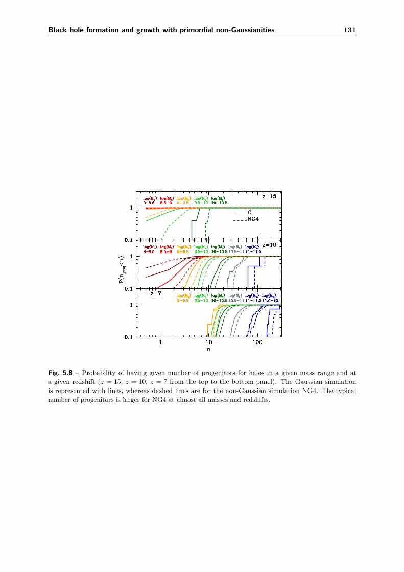
Black hole formation and growth with primordial non-Gaussianities 131

Fig. 5.8 – Probability of having given number of progenitors for halos in a given mass range and ata given redshift (z = 15, z = 10, z = 7 from the top to the bottom panel). The Gaussian simulationis represented with lines, whereas dashed lines are for the non-Gaussian simulation NG4. The typicalnumber of progenitors is larger for NG4 at almost all masses and redshifts.

132 5.4 BH formation and growth with primordial non-Gaussianities

To account for the first source of pollution (i), we eliminate from the list of potential DCcandidates the halos which are star-forming at the current time, with the probability of beingstar-forming PSF = 0.1 as described above. To account for the second contamination (ii), weestimate the probability that a halo had a progenitor which was star-forming in the past. Ina hierarchical theory of structure formation, halos are formed through the continuous mergingof smaller structures, which may have already encountered supernova-driven metal-enrichmentepisodes, making the present halo metal-polluted. Therefore the probability for a halo to bemetal-polluted increases with the number of their progenitors. For a halo of a given mass and ata given redshift, the number of progenitors is on average larger for NG4 (dashed curves), thanfor G. For instance, at z = 15 halos with mass 1010 − 3.16× 1010 M have a 50% probability ofhaving less than 5 progenitors in G, and a 50% probability of having less than 10 progenitors inNG4. In order to account for this effect we compute the mean number of progenitors per halo,for different halo mass bins, and redshifts, shown in Fig. 5.8. The mean number of progenitors isderived from the merger trees described in section 5.4.3.

The probability for a halo to be metal-polluted by heritage, i.e. to have metal-pollutedprogenitors PSF progenitor|Mh,z is described by:

PSF progenitor|Mh,z = PSF × 〈number of progenitors〉 |Mh,z. (5.25)

We keep as potential DC candidates only those halos which, after Monte Carlo sampling thisprobability, result metal-free.

Regarding the last source of metal pollution (iii), D14 conclude that metal pollution fromnearby galaxies, through galactic winds, could be an important aspect of the halo candidatescontamination. Including the redshift dependence of density and free-fall time in the expressionprovided by D14 for the bubble radius, in proper kpc (pkpc), of a metal polluted bubble onefree-fall time after the SF burst:

rbubble = 22 pkpc( Mh

1011 M

)1/5 (1 + z

11

)−6/5, (5.26)

while the radius rrad of the sphere where J21,LW = 100 one free-fall time after the star-formationburst scales as:

rrad =126 pkpc×

(1 + 834

(1 + z

11

)−3/2)−3/2

exp(− 83

300

(1 + z

11

)−3/2)1/2

×( Mh

1011M

)1/2 (J21,LW100

)−1/2 (fmod1

)1/2.

(5.27)

Fig. 5.9 compares the radius of the metal polluted sphere (rbubble) to the sphere (rrad) whereJ21,LW = 100 or J21,LW = 300.

A correction that accounts for galactic winds coming from nearby star-forming galaxies isthen added: if the distance between the halo we are considering as a DC candidate and a SFhalo is less than rbubble, then the candidate halo would be metal-polluted, hence not an eligibleDC region anymore. Fig. 5.9, however, shows that only halos with mass ∼ 1011M at z > 13can act as catalysts of a DC process in a nearby halo if J21,LW,crit 6 100. At lower masses andredshift the metal polluted bubble is always larger than the bubble irradiated by sufficientlyhigh UV flux. In our simulations, we do not have any halos with mass > 1011M at z ≥ 11 or> 1010M at z > 16, and for lower-mass halos at lower redshift, as shown in Fig. 5.9, the bubblesize is larger than the sphere irradiated by J21,LW = 100 or J21,LW = 300. Adding this correction,therefore, would leave no DC candidate in the simulation box.

Black hole formation and growth with primordial non-Gaussianities 133

Fig. 5.9 – Metal polluted bubble radius (black stars), and radius of the regions where J21,LW = 30 (redtriangle), J21,LW = 100 (orange squares) or J21,LW = 300 (yellow circles) vs redshift for different halomasses (109, 1010, 1011M). All quantities are computed one free-fall time after the star-formation burst.Only regions which are at a distance above the distance given by rbubble, and below the rrad are illuminatedby the given radiation intensity and are not polluted by galactic winds. For instance, halos with mass1011M at z = 15 can irradiate a nearby halo at a distance of ∼ 17 kpc with an intensity J21,LW = 100without polluting it (the metal bubble has reached only a distance of ∼ 14 kpc).

134 5.4 BH formation and growth with primordial non-Gaussianities

Fig. 5.10 – Number density of DC regions identified at a given redshift in the Gaussian (blue star symbols)and non-Gaussian (green star symbols) simulations. Blue and green stars are derived from a modelwhich does not account for direct pollution by galactic outflows, and where we use the radiation intensitythreshold J21,LW,crit = 300. Shaded areas represent the Poissonian errorbars derived from 40 realizationsof the process. The D14 results are shown in grey symbols: triangles correspond to their fiducial modelwhere J21,LW,crit = 300 and account for galactic winds pollution, circles to J21,LW,crit = 100, and stars toJ21,LW,crit = 300 without considering galactic winds pollution. Blue and green star symbols in our studycan be compared with star symbols in D14 as they use the same modeling for the radiation intensity (theonly differences being the probability of genetic pollution, and the use of an analytical model versus acosmological simulation). Errorbars represent the uncertainty of the mean value of the number density ofBHs.

Results on the number density of potential DC regions

The number density of DC regions obtained in this study is shown in Fig. 5.10, for both G andNG4. Blue star symbols represent the number density of DC regions in G and green star symbolsin NG4, using a model where we consider J21,LW,crit = 300.

In Fig. 5.10 we also reproduce the results of the three main models used in D14: trianglescorrespond to their fiducial model where J21,LW,crit = 300 and galactic wind pollution is included,circles to a model with J21,LW,crit = 100 and galactic wind pollution, and stars to a model withJ21,LW,crit = 300 without considering galactic wind pollution. Star symbols in our study and inD14 can be directly compared as they use the same modeling for the radiation intensity. Thetwo differences between the two studies are that we use a dark matter simulation to obtain thespatial distribution of halos, rather than an analytical prescription, and that we have derived theprobability for a halo to be metal-free from the mean number of progenitors (from the mergertree history) in halo mass and redshift bins, whereas D14 use an analytical prescription. Despitethese differences, our study is in good agreement with D14.

It is worth noting that our model does not include a treatment for galactic wind pollution(at the current time or in the past). If we included these effects, as discussed in section 5.4.1,we would not identify any DC regions in our simulation boxes, in either G or NG4. Indeed,if we estimate the number of DC candidates NDCBH in our simulation box from the model byD14, which includes galactic wind pollution, we find that NDCBH is less than one (NDCBH =nDCBH × Vbox ≈ 10−7 × Vbox = 0.04 with Vbox the simulation box volume).

Black hole formation and growth with primordial non-Gaussianities 135

Fig. 5.11 – Halo occupation fraction of newly formed BHs for the Gaussian (dashed blue line) andnon-Gaussian (solid green line) simulations, as a function of redshift, for the DC scenario (without takinginto account the metal-pollution from galactic winds). This is not a cumulative probability, but theprobability that a BH forms in a halo at a given redshift. Errorbars represent the uncertainty of the meanvalue of the occupation fraction.

With our model, we find that NG4 (green star symbols on Fig. 5.10) host a number density ofDC regions slightly larger than the Gaussian simulation (blue star symbols) for the whole rangeof redshifts, although the differences at the largest redshifts are within the 1 − σ uncertainty.The cumulative number density of BHs at redshift z=7.5 is 1.1× 10−5 cMpc−3 for G, while inNG4 the cumulative number density is almost twice, with 2.3× 10−5 cMpc−3. The cumulativenumber densities of the two simulations differ by more than 1− σ.

While the number density of BHs in NG4 is larger, so is the number of halos. In fact, whenwe estimate the occupation fraction of newly formed BHs, i.e., the fraction of halos as a functionof redshift where a BH is potentially formed (Fig. 5.11, this occupation fraction is not cumulative,i.e., we calculate it for newly formed BHs only) we find that the probability of a halo beingseeded with a BH is almost identical in the two simulations, although at the highest redshiftsthe occupation fraction in the Gaussian case is slightly above the non-Gaussian one. This can beexplained as follows: since the number of progenitors is larger in the non-Gaussian simulation(see Fig. 5.8), halos in the non-Gaussian simulation have a higher probability of being metalpolluted because of heritage pollution. In summary, scale-dependent non-gaussianities boost theoverall number of potential DC BHs in the Universe, but not the probability that a halo hosts ornot a BH.

In the vicinity of the two most massive halos

The analysis presented in the previous section highlights the difficulty of finding a significantnumber of DC regions. In order to have a clearer picture of the interplay between irradiationand metal-pollution in the model by D14, we focus here on the halos neighbouring the two mostmassive halos in our simulation volume. The reason for this choice is that according to the modeldescribed in section 5.4.1, only halos more massive than 1011M can provide an intensity higherthan J21,LW = 300 at a distance of 10 pkpc one free-fall time after the star formation burst.

136 5.4 BH formation and growth with primordial non-Gaussianities

Fig. 5.12 – The two most massive halos of the Gaussian and non-Gaussian simulations at redshift z=10are presented in blue dots. On the top left panel, we show a halo with a mass of 1.17× 1011 (ID 54335), onthe top right 1.65× 1011 (ID 61371), on the bottom left 1.22× 1011 (ID 104966) and no the bottom right1.75× 1011M (ID 118759). Indicative radii of 5 kpc, 10 kpc, and 15 kpc are shown with grey dashedlines in the (x, y) plane. The radiation intensity from these massive halos is shown in blue contours,the innermost area has intensity higher than J21,LW = 500, the second by J21,LW = 300 and outermostJ21,LW = 100. Finally, the projection of halos in the plane (x, y) is shown in colours indicating theradiation intensity they experience (in 3D): in green J21,LW < 100, in orange J21,LW ≥ 100, in purpleJ21,LW ≥ 300, in red J21,LW ≥ 500.

Critically, a common critical intensity value suggested by simulations (Bromm & Loeb, 2003 ;Sugimura, Omukai & Inoue, 2014 ; Latif & Volonteri, 2015 ; Regan, Johansson & Wise, 2014) isJ21,LW,crit ∼ 103.

We therefore select the two halos more massive than 1011M at redshift z = 10 in the G andNG4 simulations. These two halos match one another in the two simulations. Only these twohalos are able to produce sufficient radiation to efficiently dissociate molecular hydrogen on ∼ 20pkpc distances. We consider all the halos inside a 20 pkpc radius centred on each of the mostmassive halos and compute the radiation intensity illuminating them.

In Fig. 5.12, halos shown in red are illuminated by a radiation intensity higher than J21,LW =500. The number of halos is higher for the non-Gaussian simulation, as well as the number of halosexposed to a high radiation intensity. In NG4, which forms more low-mass halos, the potentialnumber of DC regions is increased. However, if we account for SN-driven metal-pollution usingEq. 5.26, 1 Myr after the SN explosion, the metals in the massive halo are already spread over 4pkpc. After 2 Myr, the metal-polluted sphere reaches 5-6 pkpc. At this time all halos illuminatedby a LW intensity J21,LW > 300 are inside this sphere and therefore polluted by metals, makingthe DC process unfeasible.Within the formalism we have adopted here, we can not identify a difference between G and NG4.However, this model includes several simplifications, for instance the expansion of the metalbubble in a real Universe may not be spherical, and PSF may well be a function of redshift and

Black hole formation and growth with primordial non-Gaussianities 137

halo mass. We argue that the non-Gaussian simulation, having more low-mass halos irradiatedby a strong UV flux, could represent a more favourable environment for this scenario.

5.4.2 BHs formed from the remnants of the first generation of stars.

Pop III star remnants is another popular scenario to explain the formation of BH seeds in theearly Universe (Madau & Rees, 2001 ; Volonteri, Madau & Haardt, 2003). BHs are predicted toform in metal-free mini-halos (Mh ∼ 105 M) at redshift z = 20− 30 from the remnants of thefirst generation of stars. If some of these stars are sufficiently massive ( > 260 M), BHs retainingup to half the stellar mass are formed, leading to the formation of a BH seed of ∼ 100M(Fryer,Woosley & Heger, 2001).In this section we want to estimate the number density of BHs and the fraction of halos wherea BH can form via the Pop III stars scenario for G and NG4. We stress that our simulationsdo not have the resolution needed to resolve mini-halos, therefore the following experiment canonly be used to assess trends. However, since the model we consider in this work has strongernon-Gaussianity on smaller scales (and thus on less massive halos), we can expect that theimpact of non-Gaussianities on mini-halos can be even larger than what we find (in the followingparagraphs) for more massive halos.According to the PopIII star scenario, only metal-free halos can host the first generation of stars.We therefore identify all the star-forming and metal-free halos in the two simulations using thesame approach described in section 5.4.1. The probability of a halo being star-forming is againPSF = 0.1 , identical for all redshifts, meaning that only 10% of the halos are selected in the firstplace as potential hosts of a Pop III remnant BH seed. Additionally, we ensure that these halosare not metal-polluted from the past history of the halo (heritage pollution), nor from galacticwinds coming from neighboring halos at a coeval redshift.Regarding the second aspect, we account for the probability of having a star-forming neighborPSF = 0.1 on a distance scale rbubble defined in Eq. 5.26, this distance is redshift and halo massdependent. We also consider the probability for the neighboring halos (on the same distancescale) to have spread metals in their past history, which could also have introduced metals inthe considered halo, making it ineligible to form PopIII star in a metal-free environment. Weperform 40 realizations of the model.

Fig. 5.13 represents the mean number density of potential BHs formed via the Pop III starremnant scenario for the two simulations (Gaussian in blue, non-Gaussian in green). The trendsof the two curves are similar, but NG4 hosts more BHs. The enhancement in the number densityof BHs increases with redshift, while at z = 7.5 the two curves are almost overlapping. Howeverthe cumulative number density of BHs for NG4 is again almost twice as large (G: 0.17 cMpc−3,NG4: 0.34 cMpc−3). The cumulative number density in the two cases differs by more than 1− σ.The occupation fraction of halos where BHs form via this scenario is shown in Fig. 5.14. Theblue line indicates the occupation fraction for G, and the green line NG4. We note that theoccupation fraction is almost identical for the two simulations: it is ∼ 10−1 at z = 17 and dropsto ∼ 10−2 at z = 8 before increasing again (we account for forming BHs only, not the cumulativeoccupation fraction). The Gaussian case is slightly above the non-Gaussian one. This can beexplained with the same arguments as those discussed for the DC case, and, moreover, halos inNG4 have also a number of neighbours slightly higher than halos in G, increasing the probabilityof being polluted by galactic winds. As noted above, our simulations do not resolve mini-halos,but since our model for fNL enhances the number of low-mass halos at a given redshift, therewill be more mini-halos in the non-Gaussian case, favouring the formation of PopIII stars at evenhigher redshifts than those considered here. Therefore, also at higher redshift, the number of

138 5.4 BH formation and growth with primordial non-Gaussianities

Fig. 5.13 – Number density of Pop III star remnant BHs formed at a given redshift for the Gaussian(dashed blue line) and the non-Gaussian (solid green line) simulations. Errorbars represent the uncertaintyof the mean value of the number density, the uncertainty is here too small to be seen.

BHs formed throughout the PopIII remnant scenario would be higher in the non-Gaussian caseuntil metal pollution starts dominating the environment. Our results can therefore be considereda lower limit to the enhancement in the BH population.

5.4.3 BHs in the most massive halos at z = 6.5

We now turn to exploring the possibility that the different growth histories of halos in Gaussianand non-Gaussian models affect the assembly of BHs at the high mass end. Using merger treesmade with TreeMaker, we derive the history of the most massive halos in all simulation boxesat redshift z = 6.5. From the mass evolution of these halos, we derive the evolution that ahypothetical BH in these halos could have.

To probe the cumulative effect that a different early evolution has on the BH population, weevolve the BH masses in the merger trees. Rather than assigning a BH mass simply based on thehalo mass at a given time we seed the highest redshift progenitor halos of the z = 6.5 halos withBH ‘seeds’ and evolve their mass over cosmic time adopting simple prescriptions. Our goal is toexplore how the dominant differences in halo growth histories caused by non-Gaussian initialconditions affect the assembly of the BHs. The main diagnostics will be the mean BH mass as afunction of time and the number of BHs with mass above some minimum threshold. The latterdiagnostic is important as we are currently able to detect only the most massive BHs (∼ 109 M).Even in the future, at such high redshift, we will always pick the most massive BHs, althoughthe mass threshold will decrease. For instance, the future X-ray mission ATHENA4 is expectedto be able to detect BHs with masses above 106 − 107 M up to z ∼ 8− 10 (Aird et al., 2013).

Specifically, first we analyse the merger trees of all halos with mass > 1011 M at z = 6.5 tofind the effects of non-Gaussianities. There are 125 such halos in simulation G and 133 in NG4.The main differences we find in the halo growth are in the total number of progenitors, and inthe number of mergers involving similarly sized halos, i.e., with mass ratio > 0.1 (‘major mergers’hereafter). We perform a Kolmogorov-Smirnov test (Fig. 5.15) and find that the probability that

4http://sci.esa.int/cosmic-vision/54517-athena/

Black hole formation and growth with primordial non-Gaussianities 139

Fig. 5.14 – Newly formed BH-halo occupation fraction for the Gaussian (blue line) and the non-Gaussian(green line) simulations, as a function of redshift, for the remnants of the first generation of stars scenario.As in Fig. 5.11, this is not a cumulative probability. Errorbars represent the uncertainty of the mean valueof the occupation fraction, the uncertainty is here too small to be seen.

the progenitor number distributions come from the same parent distribution is less than 10−6.The evidence for differences in the major merger distributions is weaker, with a probability of0.14, because of the small-number statistics. The mean number of progenitors for the > 1011 Mat z = 6.5 halos is 95 for model G and 120 for NG4. The mean number of major mergers is 16(G) and 20 (NG4).

We then model, in a simplified way, the evolution of hypothetical BHs over the cosmic historyof these halos. Two main factors linked to the different number of halos and progenitors in G andNG4 would influence the BH distribution (masses and number) at z = 6.5: (i) how many haloshost BHs, and (ii) the number of major mergers for merger-driven BH growth. Regarding thefirst point, it is expected that BH formation is not ubiquitous in all halos as specific conditionsare required (see sections 5.4.1 and 5.4.2 and Volonteri, 2010, for a review). Therefore, if eachhalo has a given probability of hosting a BH, the larger the number of the progenitors of a halo,the higher the probability that a halo without a BH acquires a BH through a merger with ahalo seeded by a BH (Menou, Haiman & Narayanan, 2001). Regarding the second point, majorgalaxy mergers trigger torques that destabilize the gas in a galaxy, causing nuclear inflows thattrigger BH accretion episodes (Kauffmann & Haehnelt, 2000 ; Hopkins et al., 2006). If a BH ishosted in a galaxy that experiences a larger number of major mergers, its growth will be boosted.

To test how the different merger histories of Gaussian and non-Gaussian models affect theBH growth in this way, we perform a first experiment where we assume that each halo startswith a 102M BH, and, after each major merger, the BHs also accrete at the Eddington limit,assuming a radiative efficiency of 10%, for one dynamical time (Tanaka, 2014), while the massesof the BHs in the merging halos are summed. The results are shown in Fig. 5.16, top panel.NG4 has a consistently higher mean BH mass and a higher number of BHs with mass above aminimum threshold, e.g., 104 M at z = 6.5. Simulation NG4 hosts 58 BHs with mass > 104 Mat z = 6.5, while G hosts 57. The BHs with mass > 105M are 8 and 3 respectively.

We perform a second experiment (Fig. 5.16, middle panel) where we assume that each halohas a 10% probability of hosting a 102 M BH when it enters the merger tree. We use here the

140 5.4 BH formation and growth with primordial non-Gaussianities

Fig. 5.15 – Cumulative distribution of the number of progenitors (top) and halo mergers with mass ratio> 0.1 for all halos with mass > 1011 M at z = 6.5 in the Gaussian (G, dotted blue histogram) and thenon-Gaussian (NG4, green, solid histogram) simulations. The probability that the progenitor distributionscome from the same parent distribution is less than 10−6. The evidence for differences in the major mergerdistributions is weaker, 0.14.

Fig. 5.16 – Top: Evolution of the BH mass for all halos with mass > 1011 Modot at z = 6.5, assumingthat accretion is only merger-driven. Middle: assuming the probability that a halo hosts a BH is 10%,and accretion is only merger-driven. Bottom: assuming that the probability that a halo hosts a BH is10% and BHs grow in mass through random accretion. Simulations: G (blue asterisks); NG4 (green stars).Each halo is represented by a point at each simulation output, and we calculate mean and variance ateach output redshift (shown as a larger point with errorbar).

Black hole formation and growth with primordial non-Gaussianities 141

occupation fraction of the Pop III star remnant case in order to have some statistics. We notethat if we increased the seed mass by a given factor, the results shown below would scale by thesame factor. Given the results of sections 5.4.1 and 5.4.2, we adopt the same probability forboth G and NG4. If the main halo already hosts a BH, the masses of the BHs in the main andmerging halo are summed. BHs also accrete at the Eddington limit for one dynamical time aftereach major merger. Simulation NG4 has 12 BHs with mass > 104 M at z = 6.5, while G has 3.Above 105 M are 1 and 0 respectively. By z = 6.5 80% of the halos host a BH in G, while thisfraction is 90% for NG4, despite starting with the same occupation fraction of 10% in each case(see Menou, Haiman & Narayanan, 2001).

The final experiment is to forego major-merger driven accretion and assign to each BHan accretion rate based on a distribution probability calculated in a large scale cosmologicalsimulation, Horizon-AGN (Dubois et al., 2014). In Fig. 5.16, bottom panel, we show a modelwhere we assume that each halo has a 10% probability of hosting a 102 M BH when it entersthe merger tree, and if the main halo already hosts a BH, their masses are summed. The BHsalso accrete over a timestep with an accretion rate randomly drawn from the distribution ofEddington rate, λ, calculated from all the BHs at 6 < z < 8 in the Horizon-AGN simulation:dN/dlogλ = 10(logλ+2)/102. In this case, simulation NG4 hosts 67 BHs with mass > 104 M atz = 6.5 while G hosts 51. The BHs with mass > 105 M are 10 and 9 respectively. Again, atz = 6.5 80% of the halos host a BH in G, while this fraction is 90% for NG4.

The main conclusion is that in NG4 the number of the most massive BHs is larger, and themean BH mass at z = 6.5 increases by 0.08, 0.22 and 0.36 dex for the third, first and secondexperiment respectively. In the Eddington rate formalism, a mass difference of a factor of twocorresponds to a change in the growth time of 70%, because of the exponential dependence.While in all the experiments the statistical significance of the difference between G and NG4 islow (they are compatible within 1− σ) the trends are always consistent: if all conditions for BHgrowth are equal, i.e., BH physics is the same, a population of BHs in NG4 would grow fasterand have more more massive BHs. In the example shown here, however, the small high-redshiftseeds do not grow much more than to a few ×105 M at z = 6.5. We have tested the differencewith a case where the initial seed mass is 105 M (keeping all other assumptions equal), andwe find that, in that case, BHs can grow up to several 108 M, less than the masses of z > 6quasars. This is not surprising, given the absence, in our simulation box, of the sufficientlymassive dark matter halos, ∼ 1013 M expected to be hosting these extremely massive BHs. Toexplain the observed quasars, with mass > 109 M, large seeds or additional growth channels(e.g., super-Eddington accretion), and sustained accretion at the Eddington level (Di Matteoet al., 2012 ; Dubois et al., 2012b) would be needed.

5.4.4 Conclusions

In this section, we have addressed the formation and the growth of supermassive BHs in thepresence of scale-dependent non-Gaussianities. We use two identical simulations except fortheir initial conditions, with either Gaussian or scale-dependent non-Gaussian primordial per-turbations (fNL(k) = fNL,0 (k/k0)α, with α = 4/3 and fNL,0 = 104). The introduction of thesenon-Gaussianities on galactic scales, consistent at larger scales with the Planck results, producesan enhancement in the low-mass end of the halo and galaxy mass functions, increasing withredshift. As a consequence, changes in the BH population arise as well. We explore the impact ofscale-dependent non-Gaussian primordial perturbations on two models of BH formation, and onthe growth of the putative BHs. Sherkatghanad & Brandenberger (2015) also investigate local-type non-Gaussianities, i.e. with both skewness (fNL) and kurtosis (described by the parameter

142 5.4 BH formation and growth with primordial non-Gaussianities

gNL), in the context of BH formation. They do not include scale-dependent non-Gaussianities,and conclude that non-Gaussianities do not strongly affect the number density of dark matterhalos at high redshifts (and of BHs as a consequence). This is in agreement with our previouswork (Habouzit et al., 2014) where we showed that non-Gaussian models closest to a non-scaledependent fNL do not show significant differences in halo and stellar mass functions comparedto the Gaussian model. On a related note, Hirano et al. (2015) find that varying the slope ofthe primordial power spectrum impacts the formation of structures as well: an enhanced powerspectrum at small length scales (or blue-tilted power spectrum) pushes to the formation of thefirst stars at much higher redshifts, and the higher CMB temperature leads to more massivestars, which can be precursor of massive BHs.

The formation of DC BHs is predicted to happen in metal-poor regions illuminated by aUV radiation intensity higher than a critical value (here we use J21,LW,crit = 100). We haveimplemented a model to identify these regions, inspired by D14, to compute the radiationintensity emitted from galaxies forming in dark matter halos. The increase in the galaxy massfunction, particularly at the low-mass end, in the non-Gaussian simulation leads to a largernumber density of potential DC regions. This is due to the increase of the number of galaxies fortwo reasons, there are statistically more regions that can collapse forming a BH, but also becausemore galaxies can act as radiation sources to illuminate dense regions where the collapse mayhappen. Conversely, the presence of more galaxies can also lead to a stronger metal enrichment,making a halo unavailable for the DC process. This last aspect has been difficult to study: wehave implemented a model for the metal-pollution coming from close star-forming regions, in thecurrent time and the past history of the regions. Taking into account the pollution coming fromgalactic winds reveals a metal pollution of all the previously identified DC regions, making anycomparison between the Gaussian and non-Gaussian simulations impossible. A larger simulationbox would be needed to test in further detail the impact of the enhancement in the low-massend of the galaxy mass function on the metal-enrichment of potential DC regions by galactic winds.

However, as the critical value for the radiation intensity is still highly debated, and may be ashigh as J21,LW,crit = 103, only halos as massive as 1011M or larger could provide sufficiently highradiation to suppress molecular hydrogen in their neighbourhood. The number of neighboursin the vicinity of the two halos more massive than 1011M in the non-Gaussian simulation islarger, up to a factor 4, for halos seeing a radiation intensity > J21,LW = 500 in the exampleshown in Fig. 5.12. This illustrates the effect of primordial non-Gaussianities in increasing thenumber density of DC regions. Metal pollution remains, however, a concern. Two factors mayalleviate the importance of metal pollution: in the first place, SN bubbles may not be spherical,as assumed in D14 and our calculation, once a realistic gas and DM distribution is taken intoaccount. Additionally, we and D14 have assumed, following Madau, Ferrara & Rees (2001) asimplified evolution of the bubble radius (see also section 5 in D14). A third approximation weand D14 have made is that the probability of a halo being star-forming is constant with redshiftand halo mass.

A second path for BH formation we have explored hinges on the remnants of the firstgeneration of stars, in metal-free mini-halos. In order to test the impact of primordial densityperturbations on this scenario, we have modified the scheme we have adopted for the directcollapse scenario (same probability for a halo to be star-forming, and the same contributionsfor the metal-pollution, namely pollution from heritage of the considered halo itself, and from

Black hole formation and growth with primordial non-Gaussianities 143

galactic winds coming from neighboring star-forming halos). Only star-forming and metal-freehalos are considered as eligible site to form BHs. While our simulations have a much lowerresolution than needed to resolve mini-halos, we can at least identify some trends. We findthat non-Gaussianities do not have a strong effect on the newly formed BH-halo occupationfraction, in both cases the occupation fraction drops from 10−1 at z = 20 to 10−2 at z = 8.Conversely, the number density of BHs is increased at the highest redshifts in the presence of non-Gaussianities, up to one order of magnitude. The larger number of progenitors and neighbours inthe non-Gaussian simulation imply a larger probability for a halo to be/become polluted by metals.

The growth of supermassive BHs is also altered when considering non-Gaussianities. Afterderiving the merger history of the most massive halos at z = 6.5 in both the Gaussian andnon-Gaussian simulations, we study the evolution of BHs in massive halos down to z = 6.5. Toinvestigate the cumulative effect over cosmic times on the BHs assembly, we model the growth ofBHs in three different ways. Different probabilities for a halo of hosting a seed BH, and differentaccretion models (either each BH accretes at the Eddington limit for a dynamical time aftera major merger or using an accretion rate based on a distribution probability derived from alarge-scale hydrodynamical simulation) are adopted. We have not included in our models theeffects of “kicks" caused by asymmetric emission of gravitational waves, which have been proposedto be possibly responsible for ejecting BHs from halos with shallow potential wells, thus haltingor reducing the growth of high-redshift BHs hosted in small halos (e.g. Yoo & Miralda-Escudé,2004 ; Volonteri & Rees, 2006 ; Tanaka & Haiman, 2009). This effect, however, seems to affect lessthan 10% of binaries and it becomes negligible for BH mergers at z < 10 (Volonteri & Rees, 2006).We find that non-Gaussianities imply a larger number of massive BHs and also an increase in themean BH mass (up to 0.36 in the most favourable experiment). A population of supermassiveBHs will then grow faster and to higher masses in a universe with scale-dependent non-Gaussianprimordial density fluctuations. If the seed masses are similar to those of PopIII star remnants,BHs will not be able to grow above few ×105 M by z = 6. However, our simulations do notresolve mini-halos, and we may underestimate the growth of seeds at earlier times. We arguethat, in a simulation resolving mini-halos, BHs would have formed earlier through the PopIIIremnant scenario, leading to a longer time for them to grow in mass. If we assumed that PopIIIremnant seeds with mass 100 M form at z ∼ 30 in halos unresolved in our simulations, theywould have grown, assuming, optimistically, constant growth at the Eddington rate (but seeJohnson & Bromm, 2007 ; Alvarez, Wise & Abel, 2009 ; Milosavljević, Couch & Bromm, 2009 ;Park & Ricotti, 2011) to ∼ 103 M by z = 18, where we start our analysis. The final BH massat z = 6 would then be ∼ one order of magnitude larger, a few ×106 M, still short of the ∼ 109

M required. The very limited growth obtained for the PopIII remnant case suggests that largeseeds or super-Eddington accretion (see Volonteri, Silk & Dubus, 2015, and references therein)may be necessary for successful BH growth. We have done the same experiments on BH growthstarting with initial 105 M BH masses (not shown here, but see section 5.4.1). In this casewe found that it is much easier for BHs to grow to higher BH masses, but still only to several108 M. This is not unexpected, because our simulation box does not contain the very rare andbiased dark matter halos with masses ∼ 1013 M believed to be hosting these extreme BHs.

Note:The relative coherent motions between baryons and dark matter, that we call streaming, could inprinciple affect the formation of supermassive black holes by both the popIII remnant scenarioand the direct collapse one. Indeed, the star formation can be delayed by few Myr in mini halos,

144 5.4 BH formation and growth with primordial non-Gaussianities

the abundance of popIII star regions can also be decreased because the virial mass needed for H2cooling is increased. The delay in star formation can favor the direct collapse scenario. However,Latif, Niemeyer & Schleicher (2014) use simulations of halos with different streaming velocitiesand show that for halos more massive than 107 M, the effect is negligible (it is more difficult forthe gas to escape from a deep potential well) compared to mini-halos. Our simulations do notresolve mini-halos, and in any case we expect the impact of streaming velocities to be the samein the Gaussian and non-Gaussian simulations. Also, the conditions where streaming velocitiescan have an impact on the BH formation are very rare (very high velocity >90 km s-1, and sovery high redshift as the streaming velocity decays with time), therefore the consequences onblack holes formation are, in conclusion, thought to be small, and should not affect the differencefound in the number density of black holes between the Gaussian and non-Gaussian simulations.Regarding the growth of supermassive black holes, streaming velocities are also thought to havea negligible effect (Greif et al., 2011 ; Naoz, Yoshida & Gnedin, 2013 ; Tanaka, Li & Haiman,2013).

Chapter 6Conclusions

The main subject of this thesis is the formation of supermassive BHs. The thesis aims atunderstanding the population of BHs in today’s galaxies, and to determine their properties, byanswering some of the following questions. Why do some galaxies host a BH, and some otherslack BHs? What is the minimum mass of a BH? What are the physical processes responsible forthe formation of BHs? What is the minimum galaxy mass where a BH can be found? How manylow mass BHs exist in the high redshift Universe? Can we explain the population of BHs in localgalaxies, or the population of high redshift quasars with the current theoretical BH formationmodels?During the last three years, I explored BH formation in the early Universe, I particularly focussedon the three following aspects:

• I have studied the formation of BHs in low-mass galaxies, which constitute the mostpromising laboratory of pristine environment we can observe today. I have presented theresults of this investigation in chapter 3.

• In the second part of this thesis, in chapter 4, I have explored the feasibility of the DC BHformation model.

• BH formation and growth has been studied in a cosmology with non-Gaussian primordialdensity perturbations in chapter 5.

In the following, I will briefly summarize the purpose of these investigations, and the differentresults we have obtained, and suggest some future extensions. During my thesis, I implemented,performed and analyzed full-physics cosmological hydrodynamical simulations with the code Ram-ses, which is a hydrodynamical adaptive mesh refinement code. For the last project (chapter 5),I analyzed a set of 5 cosmological simulations, run with the code Gadget 2, which is a smoothedparticle hydrodynamics code. We have explained the main features of these two codes in chapter 2.

Supermassive black holes are found in many galaxies, from massive galaxies to dwarf galaxies,when some other galaxies seem to not host BHs. BHs are not only present in our local Universe,the observation of quasars, powerful objects powered by massive BHs, have confirmed the presenceof BHs in the early Universe too, less than 1 Gyr after its beginning. The observation of quasarsin the early Universe, gave us the first insight of BH formation: BHs must have been formed inthe early Universe to acquire masses above a billion solar masses within 1 Gyr.

Today, our ability of observing the Universe is increasing, we are pushing the observationallimits, both in terms of local low-mass galaxies, and high redshift galaxies. We are in a promising

145

146

period, where observations will provide us new constraints on BH formation. Low-mass galaxiesare among the most pristine galaxies that we can observe locally, and therefore they can provide uscrucial information on BH formation, in analogy with “galactic archeology" for metal enrichmentand star formation histories. BH seeds form in the very early stages of the Universe, most of theirinitial properties are erased by accretion, dynamics and mergers of their host galaxies. Dwarfgalaxies, which are thought to experience a quieter growth history, may have conserved theinitial properties of BHs. Moreover low-mass galaxies can also help us to distinguish among BHformation scenarios by two main diagnostics: BH mass measurement is a direct clue of the initialBH seed mass, and the occupation fraction of these galaxies is predicted to differ for differentBH formation models.

However, the modeling of BH formation processes in simulations is still limited. For example,most of the cosmological state-of-the-art simulations seed only massive halos with a fixed BHmass of ∼ 105 M. We have, instead, implemented a new method to seed cosmological simulationsin the code Ramses, based on local environment properties, following theoretical prescriptionsof the PopIII remnants and nuclear stellar clusters BH formation models. BH form in dense,collapsing, bound, and metal-poor regions. The code computes the mass of each BH individually,according to the density of the region, and a given IMF of PopIII stars.

To test our BH formation model against observations, we have compared our simulated BHsample to the local sample of Reines & Volonteri (2015) (z 6 0.055). With this comparison,we have seen that our high redshift simulated BHs connect to the low redshift sample of localBHs. However, some of the simulated BHs are stuck at low-mass, some of them however are ableto grow up to ∼ 106 M by redshift z = 3 and to connect the observations. We find that SNfeedback has a strong impact on the formation and early growth of the simulated BHs. A strongerSN feedback implementation produces galaxies with stellar masses closer to those predicted bythe relation with halo mass, derived by the empirical model of Behroozi, Conroy & Wechsler(2010). BHs in low-mass galaxies, under the impact of such strong SN feedback, clearly have avery hard time to grow, because these galaxies have shallow potential wells, and SN feedbackis sufficient to energize gas and suppress gas accretion onto BHs. Our BH formation model,combined with the prescription of the strong SN feedback, seems to be in better agreement withthe AGN luminosity function and the lack of AGN detections in high redshift galaxies (Willottet al., 2010b ; Weigel et al., 2015).

Furthermore, the hard X-ray luminosity of the most luminous BHs in our simulated sample,is similar to the luminosity of six Lyman-Break Analogs (Jia et al., 2011b). Properties of LBAs,are very similar to their high redshift analogs, the Lyman Break Galaxies, in terms of metallicity,morphology, star formation, etc. Therefore LBAs could be a promising new laboratory for us tostudy the properties of BHs in galaxies, which look like primordial ones, but are much closer tous, thus easier to observe in detail. Our comparison, as it is today, is obviously lacking statistics,but we would like to continue investigating the comparison between our BH formation model andthe LBAs population. This comparison would help us to investigate in more detail the populationof BHs in LBGs. Generally very few AGN are observed in these galaxies. The identification ofAGN in LBGs is difficult even for those that show AGN signatures, e.g. the detection of CIV orHeII can hint either a low-luminosity AGN, as well as a population of hot young stars (Starket al., 2015 ; Pallottini et al., 2015), the same problem is actually observed for LBAs. Indeedthese galaxies often show evidences for composite system, intense starburst or/and obscuredAGN, making the AGN signatures questionable. The next step with my simulations, would beto predict the number of BHs in LBGs, and to estimate the optical and X-ray signal over starformation rate, using theoretical spectra (Feltre, Charlot & Gutkin, 2016). It will certainly help

Conclusions 147

us to understand why AGN have not been observed (yet?) in LBGs. BHs in these galaxies couldbe absent, or at least very faint and therefore not easily observable, as the BHs that remain atlow mass in our simulations.

Over the last decade, the direct collapse BH formation model has become more popular,and subject of several investigations. This scenario is appealing, as it predicts the formation ofmassive BH seeds, of ∼ 104 − 106 M in the early Universe, thus helping explaining the presenceof the billion solar mass BHs powering quasars at z > 6. In this thesis, we have studied theisothermal collapse variant of the DC model, which requires that the halo has reached the atomiccooling threshold, the absence of efficient coolants to avoid the fragmentation of the gas, and alarge inflow rate at the center of the halo. This makes the formation of BH through this channela rare event. To study the feasibility of the DC model, we have developed a hybrid model, whichcombines a model to compute the radiation intensity seen by every halos, and hydrodynamicalsimulations (taking advantage of the self-consistent evolution of metallicity, halo history, halospatial distribution). We have performed a set of simulations with a large range of simulationbox sizes, and resolutions, that allowed us to investigate different aspects of the scenario: thenumber density of direct collapse regions, but also the properties of these regions (host halomass, metallicity and metal-enrichment of halos, clustering of the regions) and the impact ofSN feedback. DCBH regions are identified by computing the local varying radiation intensity,following (Agarwal et al., 2012), and by verifying the conditions required by the theoreticalmodel.

We found that SN feedback has a crucial role in the stellar formation and in the spread ofmetals by SNe, and that it strongly impacts the number of regions eligible as DCBH sites. Withour strong implementation of SN feedback no DCBH region are identified in the 10 cMpc boxlength simulation, 3 candidates are identified with the weak SN feedback. Metal pollution ofhalos is therefore crucial, as well as the radiation intensity needed to maintain a sufficiently lowmolecular hydrogen fraction in order to avoid the fragmentation of the gas. The large scalestate-of-the-art cosmological simulation Horizon-noAGN offered us the possibility of discussingthe feasibility of the DC model in a more global fashion, at the expense of resolution. It allowedus to explore a larger range of critical radiation intensity values (Jcrit = 30, 100, 300). The mainpoint here was to understand if the population of high redshift quasars that we observe at z = 6could have been powered by DCBHs. We found that slightly less than a third of halos moremassive than 1011 M at z = 6, have a high redshift progenitor eligible for the DCBH process,considering Jcrit = 30. However, the number of halos at z = 6, which could host a DCBH, dropssignificantly if we consider higher radiation intensity (Jcrit = 100, 300).We can summarize our results by saying that if the DC model requires halos to be illuminatedby high radiation intensity of Jcrit = 300, the number of DCBHs may perhaps be sufficientto explain the population of high redshift quasars, but not the presence of DCBHs in normalgalaxies. However, if less radiation intensity is required (Jcrit = 30), and under the assumptionof weak SN feedback, then DCBHs could be common in normal galaxies.

One caveat of the hybrid models today, is that the analysis of the LW radiation distributionis done in post-processing, and BHs are actually not formed on-the-fly in the simulation. Onecan not follow these BHs over time self-consistently within the simulation. We are planningto implement in the code Ramses the DC scenario, based on the same properties as for thepresent post-processing study. This will require a larger simulation box, and a better dark matterresolution. We will be able to study what is missing in hybrid models, namely the growth ofDCBHs, their clustering/spatial distribution, but also their feedback on their host galaxies, and

148

the properties of these host galaxies. This will give us crucial clues on whether the DC modelcan reproduce/probe the population of high redshift quasars, and in normal galaxies, and howthey evolve through cosmic time.

In the last part of this thesis, we have addressed the impact of changing the cosmology onBH formation and growth. The Planck mission recently provided unprecedented accuracy ofthe estimated cosmological parameters, and of the local non-Gaussian parameter fNL, whichdescribes the deviation of initial density perturbations to a Gaussian distribution. Planck has,however, focused on large scales, mapping the CMB on the full sky, and therefore consideredprimordial density perturbations on the scale of clusters. However, some inflationary modelspredict non-Gaussianities on smaller scales, beyond the reach of CMB measurements.

In this thesis, we investigated the presence of non-Gaussinities on galactic scales, by running 5different simulations, with either Gaussian or scale-dependent non-Gaussian initial conditions, allconsistent with Planck’s constraints at large scales. The presence of non-Gaussianities on galacticscales lead to the formation of more low-mass dark matter halos, this enhancement propagatesto the galaxy mass function, with an increase at the low-mass end of the distribution. Theenhancement in the halo and galaxy mass function, depends on the prescription of the parameterfNL (in normalization and slope). The enhancement is small, but eventually detectable, it reaches0.3 dex in the low-mass end of the galaxy luminosity function at z = 10. We have shown thatthe presence of these non-Gaussianities also have strong consequences on the reionization historyof the Universe: the ionized fraction of the Universe is higher compared to the simulation withGaussian initial conditions, at the same redshift. Because of the large uncertainties of differentparameters, and the difficulty to accurately model them, such as the escape fraction or thefar-UV magnitude limit, we cannot easily favour or rule out a cosmology including non-Gaussianprimordial fluctuations. For example, all our models fit within the uncertainty of Planck’sThomson scattering measurement.

We have also used our set of numerical simulations to investigate the formation of BHsthrough the PopIII remnants and the DC models. For the DC model, we modeled the localvarying radiation intensity, combined with theoretical predictions of the scenario, to compute thenumber of eligible regions for the DC model. We found that the increase in the halo clustering,led to an enhancement in the number of DCBH regions by a factor of 2. Recent improvementson the DC BH formation model tend to conclude that this model is very rare. For example, theimpact of X-rays could significantly decrease the number density of BHs (Inayoshi & Omukai,2011 ; Latif et al., 2015). The presence of non-Gaussianities seems, instead, to boost the feasibilityof the model (see also Hirano et al., 2015 ; Sherkatghanad & Brandenberger, 2015). Similarly, forthe PopIII remnants model, we found that the presence of primordial non-Gaussianities booststhe number density of BHs by one order of magnitude at high redshift. However, the BH numberdensity in the Gaussian simulation catches up with the non-Gaussian one at later times, anderase the difference in the BH formation. PopIII remnant BHs form in metal-poor regions, and inthe non-Gaussian simulation the probability for a halo to be polluted is larger due to the highernumber of progenitors. The occupation fraction in the Gaussian and non-Gaussian simulationsremain the same for both BH formation scenarios. We found that non-Gaussianities also impactBH growth, indeed the mean mass of BHs in the non-Gaussian simulations and the number ofthe most massive BHs at z = 6.5 are both increased by a factor 2, which may be consideredhelpful in explaining how billion solar masses BHs got in place by z ∼ 6− 7.

Appendix AMonitorat at Palais de la Découverte

During my PhD, I also worked at the Palais de la Découverte, which is the museum of sciencein Paris. The museum was built in the 1930s, with the main goal of making science availablefor everyone. For this purpose, permanent expositions are presented in different fields, such asastrophysics, biology, mathematics, but also temporary expositions, where scientists are asked toexplain their current research, or the upcoming spatial missions, for example. For three years, Igave conferences on supermassive black holes every week end, for a large audience from childrento senior people. I also wrote two publications for the review Découverte of the museum, whichare listed below.

List of publications

• Les trous noirs: monstres massifs de l’UniversHabouzit, M.2016, Découverte N399

• Les ondes gravitationnelles: le cas GW150914Habouzit, M.2016, Découverte N407

Fig. A.1 – Palais de la Découverte - Paris museum of science.

149

150

Fig. A.2 – Cover of the magazine Découverte N399.

Monitorat at Palais de la Découverte 151

152

List of Figures

1 Sample of BHs in local galaxies in light and dark blue points. BH masses rangefrom few 104 M to 1010 M. The shaded area represent the domain of BH massat their formation time, in the early Universe. . . . . . . . . . . . . . . . . . . . . ii

1.1 Mass needed to collapse and form luminous objects at a given redshift (Tegmarket al., 1997). . . . . . . . . . . . . . . . . . . . . . . . . . . . . . . . . . . . . . . . 11

1.2 Relation between BH mass and the total stellar mass of local host galaxies (Reines& Volonteri, 2015). . . . . . . . . . . . . . . . . . . . . . . . . . . . . . . . . . . . 15

1.3 Low-mass BHs detected in galaxies (Volonteri) . . . . . . . . . . . . . . . . . . . 171.4 Relation between BH mass and the velocity dispersion of the host galaxy, from

Tremaine et al. (2002), and McConnell & Ma (2013) 10 years later. . . . . . . . . 211.5 SN and AGN feedback (Silk & Mamon, 2012). . . . . . . . . . . . . . . . . . . . 231.6 Theoretical growth of high redshift quasars. . . . . . . . . . . . . . . . . . . . . . 261.7 Cooling curves for primordial and metal-enriched compositions of the gas. . . . . 301.8 The fate of primordial stars (zero metallicity, non-rotating), from Heger et al. (2003). 321.9 Number density of DCBHs from Dijkstra, Ferrara & Mesinger (2014). . . . . . . 381.10 BH occupation fraction diagnostic (Greene, 2012). . . . . . . . . . . . . . . . . . 401.11 BH occupation fraction derived by Miller et al. (2015). . . . . . . . . . . . . . . . 42

2.1 Oct-tree structure of the code Ramses. . . . . . . . . . . . . . . . . . . . . . . . 472.2 Principe of the Cloud-In-Cell interpolation scheme. The particle is associated to

its corresponding cell, which is the cell overlapping the most with the particlecloud. Particle mass is distributed to the neighboring cells, proportionally to theparticle cloud area overlapping them. . . . . . . . . . . . . . . . . . . . . . . . . . 49

2.3 Polytropic equation of state . . . . . . . . . . . . . . . . . . . . . . . . . . . . . . 54

3.1 Stellar-halo mass relation for the SuperChunky simulations. . . . . . . . . . . . . 653.2 Number of BHs formed in the three simulations SuperChunky. . . . . . . . . . . 663.3 Initial mass function of BHs in SuperChunky simulations. . . . . . . . . . . . . . 673.4 Gas density (left) and metallicity (right) maps at z ∼ 10 for the delayed cooling

SN feedback simulation. . . . . . . . . . . . . . . . . . . . . . . . . . . . . . . . . 683.5 Cumulative BH mass function for the SuperChunky simulations. . . . . . . . . . 693.6 Total halo mass function, and mass function of halos hosting BHs. . . . . . . . . 703.7 Probability that a galaxy of a given mass at a given redshift hosts a BH. . . . . . 713.8 Normalized distribution of Eddington ratios log10(MBH/MEdd). . . . . . . . . . . 723.9 BH mass as a function of the total galaxy stellar mass for the simulations Super-

Chunky. . . . . . . . . . . . . . . . . . . . . . . . . . . . . . . . . . . . . . . . . . 743.10 BH growth of the most massive BHs, MBH > 106 M at z = 3. . . . . . . . . . . 743.11 Luminosity function of simulated BHs, and comparison with observations. . . . . 76

153

154 List of Figures

3.12 BH hard X-ray luminosity from the simulations SuperChunky. . . . . . . . . . . 773.13 Black hole growth of one of the most massive BH at z = 3. . . . . . . . . . . . . 803.14 Black hole growth of one of the most massive BH at z = 3. . . . . . . . . . . . . 813.15 Black hole growth of one of the most massive BH at z = 3. . . . . . . . . . . . . 823.16 Different X-rays surveys, including the new surveys ATHENA and X-ray Surveyor. 83

4.1 Gas density maps representing the three simulations used in this work: Tiny(Lbox = 1 cMpc, top panel), Chunky (Lbox = 10 cMpc, middle panel), andHorizon-noAGN (Lbox = 142 cMpc. . . . . . . . . . . . . . . . . . . . . . . . . . . 91

4.2 Top panel: median stellar mass enclosed in a sphere with a radius of 50 ckpcaround halos. Bottom panel: median of the average metallicity of halos in thetwo Chunky simulations, at redshift z = 7.33. . . . . . . . . . . . . . . . . . . . . 94

4.3 Top panel: stellar mass (solid lines), stellar mass in young stars (dashed lines) inthe neighborhood of the candidate (in a sphere of 350 ckpc radius). Bottom panel:the radiation intensity (dots) seen by the candidate halo for the two supernovafeedbacks. . . . . . . . . . . . . . . . . . . . . . . . . . . . . . . . . . . . . . . . . 96

4.4 Number density of halos that can host a DCBH, at a given redshift, and comparisonwith previous works. . . . . . . . . . . . . . . . . . . . . . . . . . . . . . . . . . . 99

4.5 Radiation intensity (in JLW units) provided by a source at a given distance (inproper kpc) for different sources mass at z = 10. . . . . . . . . . . . . . . . . . . 102

4.6 Contour plot representing the metallicity (log10 of the absolute metallicity) aroundthe SN explosion in the simulation Tiny at redshift z =10.11, 9.00, 8.09 (top tobottom). The black circle marks the analytical estimate by D14. . . . . . . . . . 105

4.7 Fraction of metal below a given mean halo metallicity, Z < 10−4 Z in blue,Z < 10−5 Z in green, Z < 10−5 Z in red, and finally Z = 0 in black. Publishedin (Latif et al., 2016). . . . . . . . . . . . . . . . . . . . . . . . . . . . . . . . . . 108

5.1 Representation of the closed triangles formed by the three momenta (k1, k2, k3). . 1145.2 Range of scales probed for fNL parameter by different observables (LoVerde et al.,

2008). . . . . . . . . . . . . . . . . . . . . . . . . . . . . . . . . . . . . . . . . . . 1175.3 Models for the scale-dependent NG parameter f local

NL . . . . . . . . . . . . . . . . . 1195.4 Analytical predictions of the nG correction to the halo mass function. . . . . . . 1205.5 Halo and galaxy stellar mass function for the Gaussian and non-Gaussian simulations.1225.6 Ionization fraction of the Universe as a function of redshift obtained for the

Gaussian and non-Gaussian simulation. . . . . . . . . . . . . . . . . . . . . . . . 1265.7 Optical depth of electrons to Thomson scattering as a function of redshift. . . . . 1285.8 Probability of having given number of progenitors for halos in a given mass range

and at a given redshift. . . . . . . . . . . . . . . . . . . . . . . . . . . . . . . . . 1315.9 Metal polluted bubble radius (black stars), and radius of the regions where

J21,LW = 30 (red triangle), J21,LW = 100 (orange squares) or J21,LW = 300 (yellowcircles) vs redshift for different halo masses (109, 1010, 1011M). . . . . . . . . . . 133

5.10 Number density of DC regions identified at a given redshift in the Gaussian andnon-Gaussian simulations. . . . . . . . . . . . . . . . . . . . . . . . . . . . . . . . 134

5.11 Halo occupation fraction of newly formed BHs for the Gaussian and non-Gaussiansimulations, as a function of redshift, for the DC scenario. . . . . . . . . . . . . . 135

5.12 The two most massive halos of the Gaussian and non-Gaussian simulations atredshift z=10. . . . . . . . . . . . . . . . . . . . . . . . . . . . . . . . . . . . . . . 136

List of Figures 155

5.13 Number density of Pop III star remnant BHs formed at a given redshift for theGaussian and the non-Gaussian simulations. . . . . . . . . . . . . . . . . . . . . . 138

5.14 Newly formed BH-halo occupation fraction for the Gaussian and the non-Gaussiansimulations, as a function of redshift, for the remnants of the first generation ofstars scenario. . . . . . . . . . . . . . . . . . . . . . . . . . . . . . . . . . . . . . . 139

5.15 Cumulative distribution of the number of progenitors (top) and halo mergers withmass ratio > 0.1 for all halos with mass > 1011 M at z = 6.5 in the Gaussianand the non-Gaussian simulations. . . . . . . . . . . . . . . . . . . . . . . . . . . 140

5.16 Evolution of the BH mass for all halos with mass > 1011 M at z = 6.5, assumingdifferent models for the accretion. . . . . . . . . . . . . . . . . . . . . . . . . . . . 140

A.1 Palais de la Découverte - Paris museum of science. . . . . . . . . . . . . . . . . . 149A.2 Cover of the magazine Découverte N399. . . . . . . . . . . . . . . . . . . . . . . . 150

156 List of Figures

List of Tables

4.1 Simulation parameters for the four simulations used in this chapter: Tiny, the twosimulations Chunky, and Horizon-noAGN. . . . . . . . . . . . . . . . . . . . . . . 90

4.2 Number of direct collapse regions in the simulation Chunky with thermal SNfeedback, assuming that collapse requires either 10 Myr, or the full free-fall timeof the halo. For reference in Chunky with delayed cooling SN feedback, the onlycase that gives one candidate, at z = 7.33, has JLW,crit = 30 and a collapse timeof 10 Myr. . . . . . . . . . . . . . . . . . . . . . . . . . . . . . . . . . . . . . . . . 95

4.3 Number of direct collapse regions in the simulation Horizon-noAGN. . . . . . . . 994.4 Percentage of massive halos with at least one DCBH progenitor, in the simulation

Horizon-noAGN. . . . . . . . . . . . . . . . . . . . . . . . . . . . . . . . . . . . . 101

5.1 Characteristics of fNL models (eq. [5.6]) . . . . . . . . . . . . . . . . . . . . . . . 118

157

158 List of Tables

List of Publications

Valiante, R., Agarwal, B., Habouzit, M., Pezzulli, E.High redshift supermassive black hole formation models2016, PASA review, submitted

Habouzit, M., Volonteri, M., Dubois, Y.Blossoms from black hole seeds: properties and early growth regulated by supernova feedback2016, arXiv:1605.09394

Latif, M. A., Omukai, K., Habouzit, M., Schleicher, D. R. G., Volonteri, M.Impact of dust cooling on direct collapse black hole formation2016, ApJ, 823, 40

Habouzit, M., Volonteri, M., Latif, M., Nishimichi, T., Peirani, S., Dubois, Y., Mamon, G.A.,Silk, J., Chevallard, J.Black hole formation and growth with non-Gaussian primordial density perturbations2016, MNRAS, 456, 1901

Habouzit, M., Volonteri, M., Latif, M., Dubois, Y., Peirani, S.On the number density of ”direct collapse” black hole seeds2016, MNRAS, 463, 529

Volonteri, M., Habouzit, M., Pacucci, F., Tremmel, M.The evolution of high-redshift massive black holes2015, arXiv:1511.02588 - Proceeding

Chevallard, J., Silk, J., Nishimichi, T., Habouzit, M., Mamon, G.A., Peirani, S.Effect of primordial non-Gaussianities on the far-UV luminosity function of high-redshiftgalaxies: implications for cosmic reionization2015, MNRAS, 446, 3235

Habouzit, M., Nishimichi, T., Peirani, S., Mamon, G.A., Silk, J., Chevallard, J.Testing primordial non-Gaussianities on galactic scales at high redshift2014, MNRAS, 445, L129

159

160 List of Publications

Bibliography

Abel T., Bryan G. L., Norman M. L., 2002, Science, 295, 93

Abramowicz M. A., 2005, in Growing Black Holes: Accretion in a Cosmological Context, MerloniA., Nayakshin S., Sunyaev R. A., eds., pp. 257–273

Abramowicz M. A., Czerny B., Lasota J. P., Szuszkiewicz E., 1988, ApJ, 332, 646

Abramowicz M. A., Lasota J.-P., 1995, Comments on Astrophysics, 18, 141

Acquaviva V., Bartolo N., Matarrese S., Riotto A., 2003, Nuclear Physics B, 667, 119

Ade P. A. R., et al., 2015

Agarwal B., Dalla Vecchia C., Johnson J. L., Khochfar S., Paardekooper J.-P., 2014, MNRAS,443, 648

Agarwal B., Johnson J. L., Zackrisson E., Labbe I., van den Bosch F. C., Natarajan P., KhochfarS., 2015a, ArXiv e-prints, arXiv: 1510.01733

Agarwal B., Khochfar S., 2015, MNRAS, 446, 160

Agarwal B., Khochfar S., Johnson J. L., Neistein E., Dalla Vecchia C., Livio M., 2012, MNRAS,425, 2854

Agarwal B., Smith B., Glover S., Natarajan P., Khochfar S., 2015b, ArXiv e-prints

Ahn K., Shapiro P. R., Iliev I. T., Mellema G., Pen U.-L., 2008, AIP Conf.Proc., 990, 374

Aird J. et al., 2013, ArXiv:1306.2325

Albrecht A., Steinhardt P. J., 1982, Physical Review Letters, 48, 1220

Alishahiha M., Silverstein E., Tong D., 2004, Phys. Rev. D, 70, 123505

Alvarez M. A., Wise J. H., Abel T., 2009, ApJ, 701, L133

Arkani-Hamed N., Creminelli P., Mukohyama S., Zaldarriaga M., 2004, J. Cosmology Astropart.Phys., 4, 001

Assef R. J. et al., 2013, ApJ, 772, 26

Aubert D., Pichon C., Colombi S., 2004, MNRAS, 352, 376

Baldassare V. F., Reines A. E., Gallo E., Greene J. E., 2015, ApJ, 809, L14

Baldwin J. A., Phillips M. M., Terlevich R., 1981, PASP, 93, 5

Ball W. H., Tout C. A., Żytkow A. N., Eldridge J. J., 2011, MNRAS, 414, 2751

161

162 Bibliography

Barnes J. E., Hernquist L., 1996, ApJ, 471, 115

Barnes J. E., Hernquist L. E., 1991, ApJ, 370, L65

Barth A. J., Greene J. E., Ho L. C., 2008, AJ, 136, 1179

Barth A. J., Ho L. C., Rutledge R. E., Sargent W. L. W., 2004, ApJ, 607, 90

Barth A. J., Strigari L. E., Bentz M. C., Greene J. E., Ho L. C., 2009, ApJ, 690, 1031

Bartolo N., Komatsu E., Matarrese S., Riotto A., 2004, Phys. Rep., 402, 103

Becker A., Huterer D., Kadota K., 2011, J. Cosmology Astropart. Phys., 1, 6

Becker R. H. et al., 2001, AJ, 122, 2850

Begelman M. C., 2004, Coevolution of Black Holes and Galaxies, 374

Begelman M. C., 2010, MNRAS, 402, 673

Begelman M. C., Cioffi D. F., 1989, ApJ, 345, L21

Begelman M. C., Rossi E. M., Armitage P. J., 2008, Mon.Not.Roy.Astron.Soc., 387, 1649

Begelman M. C., Shlosman I., 2009, ApJ, 702, L5

Begelman M. C., Volonteri M., Rees M. J., 2006, MNRAS, 370, 289

Behroozi P. S., Conroy C., Wechsler R. H., 2010, ApJ, 717, 379

Behroozi P. S., Wechsler R. H., Conroy C., 2013, ApJ, 770, 57

Belczynski K., Dominik M., Bulik T., O’Shaughnessy R., Fryer C., Holz D. E., 2010, ApJ, 715,L138

Bellovary J., Volonteri M., Governato F., Shen S., Quinn T., Wadsley J., 2011, ArXiv e-prints

Bennett C. L. et al., 1996, ApJ, 464, L1

Bieri R., Dubois Y., Silk J., Mamon G. A., Gaibler V., 2016, MNRAS, 455, 4166

Binney J., Tremaine S., 2008, Galactic Dynamics: Second Edition. Galactic Dynamics: SecondEdition, by James Binney and Scott Tremaine. ISBN 978-0-691-13026-2 (HB). Published byPrinceton University Press, Princeton, NJ USA, 2008.

Bleuler A., Teyssier R., 2014, MNRAS, 445, 4015

Booth C. M., Schaye J., 2009, MNRAS, 398, 53

Bouwens R. J., Illingworth G. D., 2006, Nature, 443, 189

Bouwens R. J. et al., 2015, ApJ, 803, 34

Bromm V., 2013, Reports on Progress in Physics, 76, 112901

Bromm V., Ferrara A., Coppi P. S., Larson R. B., 2001, MNRAS, 328, 969

Bromm V., Kudritzki R. P., Loeb A., 2001, ApJ, 552, 464

Bibliography 163

Bromm V., Loeb A., 2003, ApJ, 596, 34

Bromm V., Yoshida N., 2011, ARA&A, 49, 373

Bruzual G., Charlot S., 2003, Mon.Not.Roy.Astron.Soc., 344, 1000

Buchner J. et al., 2015, ApJ, 802, 89

Cappelluti N. et al., 2016, ApJ, 823, 95

Carr B. J., 2003, in Lecture Notes in Physics, Berlin Springer Verlag, Vol. 631, Quantum Gravity:From Theory to Experimental Search, Giulini D., Kiefer C., Laemmerzahl C., eds., pp. 301–321

Carr B. J., Bond J. R., Arnett W. D., 1984, ApJ, 277, 445

Cattaneo A., Mamon G. A., Warnick K., Knebe A., 2011, A&A, 533, A5

Cazaux S., Spaans M., 2009, A&A, 496, 365

Chabrier G., 2003, PASP, 115, 763

Chen X., 2005, Phys. Rev. D, 72, 123518

Chevallard J., Silk J., Nishimichi T., Habouzit M., Mamon G. A., et al., 2015,Mon.Not.Roy.Astron.Soc., 446, 3235

Chon S., Hirano S., Hosokawa T., Yoshida N., 2016, ArXiv e-prints

Churazov E., Sazonov S., Sunyaev R., Forman W., Jones C., Böhringer H., 2005, MNRAS, 363,L91

Civano F. et al., 2015, ApJ, 808, 185

Collin S., Boisson C., Mouchet M., Dumont A.-M., Coupé S., Porquet D., Rokaki E., 2002, A&A,388, 771

Courant R., Friedrichs K., Lewy H., 1967, IBM Journal of Research and Development, 11, 215

Courty S., Alimi J. M., 2004, A&A, 416, 875

Crocce M., Pueblas S., Scoccimarro R., 2006, MNRAS, 373, 369

Crociani D., Moscardini L., Viel M., Matarrese S., 2009, MNRAS, 394, 133

Dalal N., Doré O., Huterer D., Shirokov A., 2008, Phys. Rev. D, 77, 123514

Desjacques V., Seljak U., Iliev I. T., 2009, MNRAS, 396, 85

Devecchi B., Volonteri M., 2009, ApJ, 694, 302

Devecchi B., Volonteri M., Rossi E. M., Colpi M., Portegies Zwart S., 2012, MNRAS, 421, 1465

Di Matteo T., Colberg J., Springel V., Hernquist L., Sijacki D., 2008, ApJ, 676, 33

Di Matteo T., Khandai N., DeGraf C., Feng Y., Croft R. A. C., Lopez J., Springel V., 2012, ApJ,745, L29

Di Matteo T., Springel V., Hernquist L., 2005, Nature, 433, 604

164 Bibliography

Dicke R. H., Peebles P. J. E., Roll P. G., Wilkinson D. T., 1965, ApJ, 142, 414

Dijkstra M., Ferrara A., Mesinger A., 2014, MNRAS, 442, 2036

Dijkstra M., Haiman Z., Mesinger A., Wyithe J. S. B., 2008, MNRAS, 391, 1961

Djorgovski S. G., Castro S., Stern D., Mahabal A. A., 2001, ApJ, 560, L5

Dong R., Greene J. E., Ho L. C., 2012, ApJ, 761, 73

Dong X.-B., Ho L. C., Yuan W., Wang T.-G., Fan X., Zhou H., Jiang N., 2012, ApJ, 755, 167

Dubois Y., Devriendt J., Slyz A., Teyssier R., 2010, MNRAS, 409, 985

Dubois Y., Devriendt J., Slyz A., Teyssier R., 2012a, MNRAS, 420, 2662

Dubois Y., Devriendt J., Teyssier R., Slyz A., 2011, MNRAS, 417, 1853

Dubois Y., Pichon C., Haehnelt M., Kimm T., Slyz A., Devriendt J., Pogosyan D., 2012b,MNRAS, 423, 3616

Dubois Y. et al., 2014, MNRAS, 444, 1453

Dubois Y., Teyssier R., 2008, A&A, 477, 79

Dubois Y., Volonteri M., Silk J., 2014, MNRAS, 440, 1590

Dubois Y., Volonteri M., Silk J., Devriendt J., Slyz A., Teyssier R., 2015, MNRAS, 452, 1502

Dvali G., Gruzinov A., Zaldarriaga M., 2004, Phys. Rev. D, 69, 083505

Edri H., Rafter S. E., Chelouche D., Kaspi S., Behar E., 2012, ApJ, 756, 73

Eisenstein D. J., Loeb A., 1995, ApJ, 443, 11

Enqvist K., Sloth M. S., 2002, Nuclear Physics B, 626, 395

Fabian A. C., 1999, MNRAS, 308, L39

Fabian A. C., Iwasawa K., 1999, MNRAS, 303, L34

Fabian A. C., Sanders J. S., Taylor G. B., Allen S. W., Crawford C. S., Johnstone R. M., IwasawaK., 2006, MNRAS, 366, 417

Fan X., 2006, New A Rev., 50, 665

Fan X., Narayanan V. K., Strauss M. A., White R. L., Becker R. H., Pentericci L., Rix H.-W.,2002, AJ, 123, 1247

Fan X. et al., 2006a, AJ, 132, 117

Fan X., Strauss M. A., Richards G. T., Hennawi J. F., Becker R. H., White R. L., Diamond-StanicA. M., 2006b, AJ, 131, 1203

Fan X., Strauss M. A., Schneider D. P., Becker R. H., White R. L., Haiman Z., Gregg M., 2003,AJ, 125, 1649

Fan X. e. a., 2001, AJ, 121, 54

Bibliography 165

Feltre A., Charlot S., Gutkin J., 2016, MNRAS, 456, 3354

Ferrarese L., 2002, ApJ, 578, 90

Ferrarese L., Merritt D., 2000, ApJ, 539, L9

Filippenko A. V., Ho L. C., 2003, ApJ, 588, L13

Friedmann A., 1922, Zeitschrift fur Physik, 10, 377

Fryer C. L., Woosley S. E., Heger A., 2001, ApJ, 550, 372

Fryxell B. et al., 2000, ApJS, 131, 273

Gaibler V., Khochfar S., Krause M., Silk J., 2012, MNRAS, 425, 438

Gallo E., Treu T., Jacob J., Woo J.-H., Marshall P. J., Antonucci R., 2008, ApJ, 680, 154

Gallo E., Treu T., Marshall P. J., Woo J.-H., Leipski C., Antonucci R., 2010, ApJ, 714, 25

Gangui A., Lucchin F., Matarrese S., Mollerach S., 1994, ApJ, 430, 447

Gebhardt K. et al., 2000, ApJ, 539, L13

Gebhardt K. et al., 2001, AJ, 122, 2469

Gorski K. M., Banday A. J., Bennett C. L., Hinshaw G., Kogut A., Smoot G. F., Wright E. L.,1996, ApJ, 464, L11

Greene J. E., 2012, Nature Communications, 3, 1304

Greene J. E., Ho L. C., 2004, ApJ, 610, 722

Greene J. E., Ho L. C., 2005, ApJ, 630, 122

Greene J. E., Ho L. C., 2007a, ApJ, 670, 92

Greene J. E., Ho L. C., 2007b, ApJ, 667, 131

Greenstein J. L., 1963, Nature, 197, 1041

Greif T. H., 2015, Computational Astrophysics and Cosmology, 2, 3

Greif T. H., Bromm V., Clark P. C., Glover S. C. O., Smith R. J., Klessen R. S., Yoshida N.,Springel V., 2012, MNRAS, 424, 399

Greif T. H., Johnson J. L., Klessen R. S., Bromm V., 2008, MNRAS, 387, 1021

Greif T. H., White S. D. M., Klessen R. S., Springel V., 2011, ApJ, 736, 147

Grossi M., Dolag K., Branchini E., Matarrese S., Moscardini L., 2007, MNRAS, 382, 1261

Grossi M., Verde L., Carbone C., Dolag K., Branchini E., Iannuzzi F., Matarrese S., MoscardiniL., 2009, MNRAS, 398, 321

Guth A. H., 1981, Phys. Rev. D, 23, 347

Haardt F., Madau P., 1996, ApJ, 461, 20

166 Bibliography

Habouzit M., Nishimichi T., Peirani S., Mamon G. A., Silk J., et al., 2014,Mon.Not.Roy.Astron.Soc., 445, 129

Habouzit M., Volonteri M., Dubois Y., 2016, ArXiv:1605.09394

Habouzit M., Volonteri M., Latif M., Dubois Y., Peirani S., 2016a, MNRAS, 463, 529

Habouzit M. et al., 2016b, MNRAS, 456, 1901

Hahn O., Abel T., 2013, MUSIC: MUlti-Scale Initial Conditions. Astrophysics Source CodeLibrary

Harrison E. R., 1970, Phys. Rev. D, 1, 2726

Hartwig T., Glover S. C. O., Klessen R. S., Latif M. A., Volonteri M., 2015, MNRAS, 452, 1233

Hartwig T. et al., 2016, MNRAS, 462, 2184

Hazard C., Mackey M. B., Shimmins A. J., 1963, Nature, 197, 1037

Heger A., Fryer C. L., Woosley S. E., Langer N., Hartmann D. H., 2003, ApJ, 591, 288

Herschel J. F. W., 1864, Philosophical Transactions of the Royal Society of London Series I, 154,1

Hirano S., Hosokawa T., Yoshida N., Umeda H., Omukai K., Chiaki G., Yorke H. W., 2014, ApJ,781, 60

Hirano S., Zhu N., Yoshida N., Spergel D., Yorke H. W., 2015

Hirschmann M., Naab T., Somerville R. S., Burkert A., Oser L., 2012a, MNRAS, 419, 3200

Hirschmann M., Somerville R. S., Naab T., Burkert A., 2012b, MNRAS, 426, 237

Hockney R. W., Eastwood J. W., 1981, Computer Simulation Using Particles

Hopkins P. F., Hernquist L., Cox T. J., Di Matteo T., Robertson B., Springel V., 2006, ApJs,163, 1

Hopkins P. F., Richards G. T., Hernquist L., 2007, ApJ, 654, 731

Hosokawa T., Omukai K., Yorke H. W., 2012, ApJ, 756, 93

Hosokawa T., Yorke H. W., Inayoshi K., Omukai K., Yoshida N., 2013, ApJ, 778, 178

Hubble E., 1929, Proceedings of the National Academy of Science, 15, 168

Hubble E. P., 1925, The Observatory, 48, 139

Inayoshi K., Haiman Z., Ostriker J. P., 2016, MNRAS, 459, 3738

Inayoshi K., Omukai K., 2011, MNRAS, 416, 2748

Inayoshi K., Tanaka T. L., 2015, MNRAS, 450, 4350

Islam R. R., Taylor J. E., Silk J., 2003, MNRAS, 340, 647

Izotov Y. I., Guseva N. G., Fricke K. J., Henkel C., 2014, A&A, 561, A33

Bibliography 167

Jarrett T. H. et al., 2011, ApJ, 735, 112

Jia J., Ptak A., Heckman T. M., Overzier R. A., Hornschemeier A., LaMassa S. M., 2011a, ApJ,731, 55

Jia J., Ptak A., Heckman T. M., Overzier R. A., Hornschemeier A., LaMassa S. M., 2011b, ApJ,731, 55

Jiang L., et al.,, 2009, AJ, 138, 305

Johnson J. L., Bromm V., 2007, MNRAS, 374, 1557

Johnson J. L., Dalla Vecchia C., Khochfar S., 2013, MNRAS, 428, 1857

Johnson J. L., Whalen D. J., Agarwal B., Paardekooper J.-P., Khochfar S., 2014, Mon. Not. Roy.Astron. Soc., 445, 686

Johnson J. L., Whalen D. J., Fryer C. L., Li H., 2012, ApJ, 750, 66

Johnson J. L., Whalen D. J., Li H., Holz D. E., 2013, ApJ, 771, 116

Kang X., Norberg P., Silk J., 2007, MNRAS, 376, 343

Katz H., Sijacki D., Haehnelt M. G., 2015, ArXiv e-prints:1502.03448

Kauffmann G., Haehnelt M., 2000, MNRAS, 311, 576

Kimm T., Cen R., 2014, ApJ, 788, 121

Komatsu E. et al., 2003, ApJS, 148, 119

Komatsu E. et al., 2011, ApJS, 192, 18

Komatsu E., Spergel D. N., 2001, Phys. Rev. D, 63, 063002

Kormendy J., Bender R., 2011, Nature, 469, 377

Kormendy J., Ho L. C., 2013, ARA&A, 51, 511

Kormendy J., Richstone D., 1995, ARA&A, 33, 581

Koushiappas S. M., Bullock J. S., Dekel A., 2004, MNRAS, 354, 292

Kravtsov A. V., Klypin A. A., Khokhlov A. M., 1997, ApJS, 111, 73

Kuhlen M., Faucher-Giguère C.-A., 2012, MNRAS, 423, 862

Lam T. Y., Nishimichi T., Yoshida N., 2011, MNRAS, 414, 289

Latif M. A., Bovino S., Grassi T., Schleicher D. R. G., Spaans M., 2015, MNRAS, 446, 3163

Latif M. A., Niemeyer J. C., Schleicher D. R. G., 2014, MNRAS, 440, 2969

Latif M. A., Omukai K., Habouzit M., Schleicher D. R. G., Volonteri M., 2016, ApJ, 823, 40

Latif M. A., Schleicher D. R. G., Bovino S., Grassi T., Spaans M., 2014, ApJ, 792, 78

Latif M. A., Schleicher D. R. G., Schmidt W., Niemeyer J., 2013a, MNRAS, 433, 1607

168 Bibliography

Latif M. A., Schleicher D. R. G., Schmidt W., Niemeyer J., 2013b, ApJ, 772, L3

Latif M. A., Schleicher D. R. G., Spaans M., 2012, A&A, 540, A101

Latif M. A., Volonteri M., 2015, MNRAS, 452, 1026

Leavitt H. S., 1908, Annals of Harvard College Observatory, 60, 87

Lemaître G., 1927, Annales de la Societe Scientifique de Bruxelles, 47, 49

Lemons S. M., Reines A. E., Plotkin R. M., Gallo E., Greene J. E., 2015, ApJ, 805, 12

Lewis A., Challinor A., Lasenby A., 2000, ApJ, 538, 473

Linde A. D., 1982, Physics Letters B, 108, 389

Lodato G., Natarajan P., 2006, MNRAS, 371, 1813

Loeb A., Rasio F. A., 1994, ApJ, 432, 52

LoVerde M., Miller A., Shandera S., Verde L., 2008, J. Cosmology Astropart. Phys., 4, 14

Lupi A., Colpi M., Devecchi B., Galanti G., Volonteri M., 2014, MNRAS, 442, 3616

Lupi A., Haardt F., Dotti M., Fiacconi D., Mayer L., Madau P., 2016, MNRAS, 456, 2993

Lyth D. H., Wands D., 2002, Physics Letters B, 524, 5

Machacek M. E., Bryan G. L., Abel T., 2001, ApJ, 548, 509

Madau P., Ferrara A., Rees M. J., 2001, ApJ, 555, 92

Madau P., Haardt F., Dotti M., 2014, ApJ, 784, L38

Madau P., Rees M. J., 2001, ApJL, 551, L27

Magorrian J. et al., 1998, AJ, 115, 2285

Maio U., 2011, Classical and Quantum Gravity, 28, 225015

Maio U., Iannuzzi F., 2011, MNRAS, 415, 3021

Maio U., Khochfar S., 2012, MNRAS, 421, 1113

Maldacena J., 2003, Journal of High Energy Physics, 5, 13

Mapelli M., Colpi M., Zampieri L., 2009, MNRAS, 395, L71

Mapelli M., Zampieri L., Ripamonti E., Bressan A., 2013, MNRAS, 429, 2298

Marconi A., Hunt L. K., 2003, ApJ, 589, L21

Matarrese S., Verde L., Jimenez R., 2000, ApJ, 541, 10

Matthews T. A., Sandage A. R., 1963, ApJ, 138, 30

Mayer L., Fiacconi D., Bonoli S., Quinn T., Roskar R., Shen S., Wadsley J., 2014, ArXive-prints:1411.5683

Bibliography 169

Mayer L., Kazantzidis S., Escala A., Callegari S., 2010, Nature, 466, 1082

McConnell N. J., Ma C.-P., 2013, ApJ, 764, 184

McConnell N. J., Ma C.-P., Gebhardt K., Wright S. A., Murphy J. D., Lauer T. R., GrahamJ. R., Richstone D. O., 2011, Nature, 480, 215

McLure R. J., Dunlop J. S., 2001, MNRAS, 327, 199

Menon H., Wesolowski L., Zheng G., Jetley P., Kale L., Quinn T., Governato F., 2015, Compu-tational Astrophysics and Cosmology, 2, 1

Menou K., Haiman Z., Narayanan V. K., 2001, ApJ, 558, 535

Merloni A., Heinz S., di Matteo T., 2003, MNRAS, 345, 1057

Merritt D., Ferrarese L., Joseph C. L., 2001, Science, 293, 1116

Messier C., 1781, Catalogue des Nebuleuses et des amas d’Etoiles (Catalog of Nebulae and StarClusters). Tech. rep.

Mezcua M., Civano F., Fabbiano G., Miyaji T., Marchesi S., 2016, ApJ, 817, 20

Miller B., Gallo E., Treu T., Woo J.-H., 2012, ApJ, 747, 57

Miller B. P., Gallo E., Greene J. E., Kelly B. C., Treu T., Woo J.-H., Baldassare V., 2015, ApJ,799, 98

Milosavljevic M., Bromm V., Couch S. M., Oh S. P., 2009, Astrophys. J., 698, 766

Milosavljević M., Couch S. M., Bromm V., 2009, ApJL, 696, L146

Mollerach S., 1990, Phys. Rev. D, 42, 313

Moran E. C., Shahinyan K., Sugarman H. R., Vélez D. O., Eracleous M., 2014, AJ, 148, 136

Mortlock D. J. et al., 2011, Nature, 474, 616

Mutch S. J., Croton D. J., Poole G. B., 2013, Mon.Not.Roy.Astron.Soc., 435, 2445

Naoz S., Yoshida N., Gnedin N. Y., 2013, ApJ, 763, 27

Nishimichi T., 2012, J. Cosmology Astropart. Phys., 8, 37

Nishimichi T. et al., 2009, PASJ, 61, 321

Nishimichi T., Taruya A., Koyama K., Sabiu C., 2010, J. Cosmology Astropart. Phys., 7, 2

Oh S. P., Haiman Z., 2002, ApJ, 569, 558

Oke J. B., 1963, Nature, 197, 1040

Omukai K., 2001, ApJ, 546, 635

Omukai K., Schneider R., Haiman Z., 2008, ApJ, 686, 801

Omukai K., Tsuribe T., Schneider R., Ferrara A., 2005, ApJ, 626, 627

170 Bibliography

O’Shea B. W., Bryan G., Bordner J., Norman M. L., Abel T., Harkness R., Kritsuk A., 2004,ArXiv Astrophysics e-prints 0403044

O’Shea B. W., Norman M. L., 2008, ApJ, 673, 14

Pace F., Maio U., 2014, MNRAS, 437, 1308

Pace F., Moscardini L., Bartelmann M., Branchini E., Dolag K., Grossi M., Matarrese S., 2011,MNRAS, 411, 595

Pacucci F., Ferrara A., Volonteri M., Dubus G., 2015, ArXiv e-prints

Pacucci F., Volonteri M., Ferrara A., 2015, MNRAS, 452, 1922

Palla F., Salpeter E. E., Stahler S. W., 1983, ApJ, 271, 632

Pallottini A., Ferrara A., Gallerani S., Salvadori S., D’Odorico V., 2014, MNRAS, 440, 2498

Pallottini A. et al., 2015

Pardo K. et al., 2016, ApJ, 831, 203

Park K., Ricotti M., 2011, ApJ, 739, 2

Peebles P. J. E., 1969, ApJ, 155, 393

Peebles P. J. E., Yu J. T., 1970, ApJ, 162, 815

Pelupessy F. I., Di Matteo T., Ciardi B., 2007, ApJ, 665, 107

Penzias A. A., Wilson R. W., 1965, ApJ, 142, 419

Perlmutter S. et al., 1999, ApJ, 517, 565

Peterson B. M. et al., 2005, ApJ, 632, 799

Pillepich A., Porciani C., Hahn O., 2010, MNRAS, 402, 191

Planck Collaboration et al., 2013a, arXiv:1303.5076

Planck Collaboration et al., 2013b, arXiv:1303.5084

Planck Collaboration et al., 2014, A&A, 571, A16

Planck Collaboration et al., 2015a, ArXiv:1502.01592

Planck Collaboration et al., 2011, A&A, 536, A1

Planck Collaboration et al., 2015b, ArXiv:1502.01589

Portegies Zwart S. F., Makino J., McMillan S. L. W., Hut P., 1999, A&A, 348, 117

Press W. H., Schechter P., 1974, ApJ, 187, 425

Rasera Y., Teyssier R., 2006, A&A, 445, 1

Redmount I. H., Rees M. J., 1989, Comments on Astrophysics, 14, 165

Rees M. J., 1978, The Observatory, 98, 210

Bibliography 171

Rees M. J., 1984, ARA&A, 22, 471

Rees M. J., 1989, MNRAS, 239, 1P

Regan J. A., Haehnelt M. G., 2009a, MNRAS, 396, 343

Regan J. A., Haehnelt M. G., 2009b, MNRAS, 393, 858

Regan J. A., Johansson P. H., Wise J. H., 2014, ApJ, 795, 137

Reines A. E., 2015, in American Astronomical Society Meeting Abstracts, Vol. 225, AmericanAstronomical Society Meeting Abstracts, p. 320.07

Reines A. E., Deller A. T., 2012, ApJ, 750, L24

Reines A. E., Greene J. E., Geha M., 2013, ApJ, 775, 116

Reines A. E., Plotkin R. M., Russell T. D., Mezcua M., Condon J. J., Sivakoff G. R., JohnsonK. E., 2014, ApJ, 787, L30

Reines A. E., Sivakoff G. R., Johnson K. E., Brogan C. L., 2011, Nature, 470, 66

Reines A. E., Volonteri M., 2015, ArXiv e-prints

Robertson B. E., Ellis R. S., Dunlop J. S., McLure R. J., Stark D. P., 2010, Nature, 468, 49

Robertson B. E. et al., 2013, ApJ, 768, 71

Schaerer D., 2002, A&A, 382, 28

Schauer A. T. P., Whalen D. J., Glover S. C. O., Klessen R. S., 2015, MNRAS, 454, 2441

Schleicher D. R. G., Palla F., Ferrara A., Galli D., Latif M., 2013, A&A, 558, A59

Schmidt M., 1963, Nature, 197, 1040

Schneider R., Ferrara A., Natarajan P., Omukai K., 2002, ApJ, 571, 30

Schneider R., Ferrara A., Salvaterra R., Omukai K., Bromm V., 2003, Nature, 422, 869

Schneider R., Omukai K., Inoue A. K., Ferrara A., 2006a, MNRAS, 369, 1437

Schneider R., Salvaterra R., Ferrara A., Ciardi B., 2006b, MNRAS, 369, 825

Schnittman J. D., 2007, ApJ, 667, L133

Schramm M. et al., 2013, ApJ, 773, 150

Scoccimarro R., 1998, MNRAS, 299, 1097

Sefusatti E., Crocce M., Desjacques V., 2010, MNRAS, 406, 1014

Seth A. C. et al., 2010, ApJ, 714, 713

Shakura N. I., Sunyaev R. A., 1973, A&A, 24, 337

Shandera S., Dalal N., Huterer D., 2011, J. Cosmology Astropart. Phys., 3, 17

Shang C., Bryan G. L., Haiman Z., 2010, MNRAS, 402, 1249

172 Bibliography

Sherkatghanad Z., Brandenberger R. H., 2015, ArXiv:1508.00968

Shih D. C., Iwasawa K., Fabian A. C., 2003, MNRAS, 341, 973

Shirasaki M., Yoshida N., Hamana T., Nishimichi T., 2012, ApJ, 760, 45

Shlosman I., Frank J., Begelman M. C., 1989, Nature, 338, 45

Sijacki D., Springel V., Haehnelt M. G., 2009, MNRAS, 400, 100

Sijacki D., Vogelsberger M., Genel S., Springel V., Torrey P., Snyder G. F., Nelson D., HernquistL., 2015, MNRAS, 452, 575

Silk J., 2013, ApJ, 772, 112

Silk J., Mamon G. A., 2012, Research in Astronomy and Astrophysics, 12, 917

Silk J., Rees M. J., 1998, A&A, 331, L1

Silverstein E., Tong D., 2004, Phys. Rev. D, 70, 103505

Slipher V. M., 1917, Proceedings of the American Philosophical Society, 56, 403

Smith H. J., Hoffleit D., 1963, AJ, 68, 292

Smith K. M., Senatore L., Zaldarriaga M., 2009, J. Cosmology Astropart. Phys., 9, 006

Smoot G. F. et al., 1992, ApJ, 396, L1

Soltan A., 1982, MNRAS, 200, 115

Somerville R. S., Hopkins P. F., Cox T. J., Robertson B. E., Hernquist L., 2008, MNRAS, 391,481

Spaans M., Silk J., 2006, ApJ, 652, 902

Spera M., Mapelli M., Bressan A., 2015, MNRAS, 451, 4086

Spergel D. N. et al., 2003, ApJS, 148, 175

Springel V., 2005, MNRAS, 364, 1105

Springel V., 2010, MNRAS, 401, 791

Springel V., Hernquist L., 2003, MNRAS, 339, 289

Springel V., Yoshida N., White S. D. M., 2001, New Astronomy, 6, 79

Stark D. P. et al., 2015, MNRAS, 454, 1393

Stern D. et al., 2012, ApJ, 753, 30

Stinson G., Seth A., Katz N., Wadsley J., Governato F., Quinn T., 2006, MNRAS, 373, 1074

Sugimura K., Omukai K., Inoue A. K., 2014, MNRAS, 445, 544

Sutherland R. S., Dopita M. A., 1993, ApJS, 88, 253

Tanaka T., Haiman Z., 2009, ApJ, 696, 1798

Bibliography 173

Tanaka T. L., 2014, Classical and Quantum Gravity, 31, 244005

Tanaka T. L., Li M., Haiman Z., 2013, MNRAS, 435, 3559

Taylor P., Kobayashi C., 2014, MNRAS, 442, 2751

Tegmark M., Silk J., Rees M. J., Blanchard A., Abel T., Palla F., 1997, ApJ, 474, 1

Teyssier R., 2002, A&A, 385, 337

Teyssier R., Moore B., Martizzi D., Dubois Y., Mayer L., 2011, MNRAS, 414, 195

Teyssier R., Pontzen A., Dubois Y., Read J. I., 2013, MNRAS, 429, 3068

Tornatore L., Ferrara A., Schneider R., 2007, MNRAS, 382, 945

Treister E., Schawinski K., Volonteri M., Natarajan P., 2013, ApJ, 778, 130

Tremaine S. et al., 2002, ApJ, 574, 740

Tremmel M., Governato F., Volonteri M., Quinn T. R., 2015, MNRAS, 451, 1868

Tweed D., Devriendt J., Blaizot J., Colombi S., Slyz A., 2009, A&A, 506, 647

Valageas P., Nishimichi T., 2011, A&A, 527, A87

Valiante R., Schneider R., Volonteri M., Omukai K., 2016, MNRAS, 457, 3356

Valluri M., Ferrarese L., Merritt D., Joseph C. L., 2005, ApJ, 628, 137

van Wassenhove S., Volonteri M., Walker M. G., Gair J. R., 2010, MNRAS, 408, 1139

Vink J. S., 2008, New A Rev., 52, 419

Visbal E., Haiman Z., Bryan G. L., 2014, MNRAS, 445, 1056

Volonteri M., 2010, A&AR, 18, 279

Volonteri M., Begelman M. C., 2010, MNRAS, 409, 1398

Volonteri M., Dubois Y., Pichon C., Devriendt J., 2016, MNRAS, 460, 2979

Volonteri M., Haardt F., Madau P., 2003, ApJ, 582, 559

Volonteri M., Lodato G., Natarajan P., 2008, MNRAS, 383, 1079

Volonteri M., Madau P., Haardt F., 2003, ApJ, 593, 661

Volonteri M., Natarajan P., 2009, MNRAS, 400, 1911

Volonteri M., Perna R., 2005, MNRAS, 358, 913

Volonteri M., Rees M. J., 2006, ApJ, 650, 669

Volonteri M., Silk J., Dubus G., 2015, ApJ, 804, 148

Volonteri M., Stark D. P., 2011, MNRAS, 417, 2085

Wadsley J. W., Stadel J., Quinn T., 2004, New Astronomy, 9, 137

174 References

Weigel A. K., Schawinski K., Treister E., Urry C. M., Koss M., Trakhtenbrot B., 2015, MNRAS,448, 3167

White R. L., Becker R. H., Fan X., Strauss M. A., 2003, AJ, 126, 1

Willott C. J. et al., 2010a, AJ, 140, 546

Willott C. J. et al., 2007, AJ, 134, 2435

Willott C. J. et al., 2010b, AJ, 139, 906

Wise J. H., Demchenko V. G., Halicek M. T., Norman M. L., Turk M. J., Abel T., Smith B. D.,2014, MNRAS, 442, 2560

Wise J. H., Turk M. J., Abel T., 2008, ApJ, 682, 745

Wolcott-Green J., Haiman Z., Bryan G. L., 2011, MNRAS, 418, 838

Wrobel J. M., Ho L. C., 2006, ApJ, 646, L95

Yoo J., Miralda-Escudé J., 2004, ApJL, 614, L25

York D. G. et al., 2000, AJ, 120, 1579

Yoshida N., Bromm V., Hernquist L., 2004, ApJ, 605, 579

Yoshida N., Omukai K., Hernquist L., 2008, Science, 321, 669

Yu Q., Tremaine S., 2002, MNRAS, 335, 965

Yuan W., Zhou H., Dou L., Dong X.-B., Fan X., Wang T.-G., 2014, ApJ, 782, 55

Yungelson L. R., van den Heuvel E. P. J., Vink J. S., Portegies Zwart S. F., de Koter A., 2008,A&A, 477, 223

Zeldovich Y. B., 1972, MNRAS, 160, 1P

Zwicky F., 1933, Helvetica Physica Acta, 6, 110

References 175