
FORTH-ICS / TR-388 April 2007
Request-Grant SchedulingFor Congestion Elimination
in Multistage Networks
Nikolaos I. Chrysos1,2
Abstract: This thesis considers buffered multistage interconnection networks
(fabrics), and investigates methods to reduce their buffer size requirements. Our con-
tribution is a novel flow and congestion control scheme that achieves performance
close to that of per-flow queueing while requiring much less buffer space than what
per-flow queues would need. The new scheme utilizes a request-grant pre-approval
phase, as many contemporary bufferless networks do, but its operation is much sim-
pler and its performance is remarkably better. Traditionally, the role of requests in
bufferless networks is to reserve an available time slot on each link along a packet’s
route, where these time slots are contiguous in time along the path, so as to guar-
antee non-conflicting packet transmission. These requirements impose a very heavy
toll on the scheduling unit of such bufferless fabrics. By contrast, our requests do
not reserve links for a specific time duration, but instead only reserve space in the
buffers at their entry points; effectively, the scheduling decisions that concern dif-
ferent links are decoupled among themselves, leading to a much simpler admission
process. The proposed scheduling subsystem comprises independent single-resource
schedulers, operating in a pipeline; they operate asynchronously to each other. In this
thesis we show that the reservation of buffers in front of critical network links –links
that are unable to carry the potential aggregate demand– eliminates congestion, in

the sense that traffic flows seamlessly through the network: it neither gets dropped,
nor is excessively blocked waiting for downstream buffers to become available.
First, we apply request-grant scheduling to a single-stage switch, with small,
shared output queues, which serves as a model for the more challenging multistage
case. We demonstrate that, in principle, a very small number of fabric buffers suffices
to reach high performance levels: with 12-cell buffer space per output, performance is
better than in buffered crossbars, which consume N cells of buffer space per output,
where N is the number of ports. In this single-stage setting, we study the impact of
input contention on scheduler performance, and the related synchronization phenom-
ena. During this work, we have introduced a novel scheduling scheme for buffered
crossbar switches that makes buffer size independent of the round-trip-time between
the linecards and the switch.
We then proceed to the multistage case. Our main motivation and our primary
benchmark is an example next-generation fabric challenge: a 1024 × 1024, 3-stage,
non-blocking Clos/Benes fabric, running with no internal speedup, made of 96 single-
chip 32× 32 buffered crosssbar switching elements (3 stages of 32 switch chips each).
To eliminate congestion in the fabric, we carefully apply our request-grant scheduling
protocol. We demonstrate that it is feasible to implement all schedulers centrally, in a
single chip. Besides congestion elimination, our scheduler can guarantee 100 percent
in-order delivery, using very small reorder buffers, which can easily fit in on-chip
memory. Simulation results indicate very good delay performance, and throughput
that exceeds 95% under unbalanced traffic. Most prominent is the result that, under
hot-spot traffic, with almost all output ports being congested, the non-congested
outputs experience negligible delay degradation. The proposed system can directly
operate on variable-size packets, eliminating the padding overhead and the associated
internal speed-up. We also discuss a possible distributed version of the scheduling
subsystem. Our scheme is appropriate to deal with heavy congestion; in systems that
need to provide very low latency under (uncongested) light traffic, one would apply
this scheme when the load exceeds a given threshold.
Lastly, we consider some blocking network topologies, like the banyan. In a banyan

network, besides output ports, internal links can cause congestion as well. We show
a fully distributed scheduler for this network, that eliminates congestion from both
internal and output-port links.
Keywords: Congestion Management, Flow Control, Flow Isolation, Small Internal
Buffers, Shared Buffers, Interconnection Networks, Non-Blocking Networks, Multi-
stage Fabrics, Benes Networks, Banyan Networks, Multipath Routing, Inverse Multi-
plexing, Load Balancing, Buffered Crossbar, Crossbar Scheduling, Pipelined Schedul-
ing, Distributed Scheduling, Credit Prediction, Scheduler Synchronization, Desyn-
chronized Schedulers, Round Robin, Weighted Round Robin
1ICS-FORTH, P.O. Box 1385, GR-711-10 Heraklion, Crete, Greece.2Department of Computer Science, University of Crete, Heraklion, Crete, Greece.

.
Request-Grant Scheduling For CongestionElimination in Multistage Networks
Nikolaos I. Chrysos1,2
Computer Architecture & VLSI Systems(CARV) Laboratory,Institute of Computer Science(ICS)
Foundation of Research and Technology Hellas(FORTH)Science and Technology Park of Crete
P.O. Box 1385 Heraklion, Crete, GR-711-10 Greeceemail: [email protected]
url: http://archvlsi.ics.forth.gr/
Technical Report FORTH-ICS/TR-388 April 2007
Copyright 2007 by FORTHWork Performed as a Ph.D Thesis at the Depart. of Computer Science, U. of Crete;
under the supervision of Prof. Manolis Katevenis,with the financial support of FORTH-ICS and an IBM Ph.D. Fellowship.
Keywords: Congestion Management, Flow Control, Flow Isolation, Small InternalBuffers, Shared Buffers, Interconnection Networks, Non-Blocking Networks, Multi-stage Fabrics, Benes Networks, Banyan Networks, Multipath Routing, Inverse Multi-plexing, Load Balancing, Buffered Crossbar, Crossbar Scheduling, Pipelined Schedul-ing, Distributed Scheduling, Credit Prediction, Scheduler Synchronization, Desyn-chronized Schedulers, Round Robin, Weighted Round Robin
1ICS-FORTH, P.O. Box 1385, GR-711-10 Heraklion, Crete, Greece.2Department of Computer Science, University of Crete, Heraklion, Crete, Greece.

Request-Grant Scheduling for Congestion
Elimination in Multistage Networks
by
Nikolaos I. Chrysos
(supervisor Prof. Manolis Katevenis)
A dissertation submitted to the faculty of
University of Crete
in partial fulfillment of the requirements for the degree of
Doctor of Philosophy
Department of Computer Science
University of Crete
December 2006
ACKNOWLEDGMENTS
I would especially like to thank professor Manolis Katevenis for giving
me the opportunity to study about “switches and switching”, a subject that I
found very interesting from the beginning. Prof. Katevenis was the person that
introduced to this subject, through the respective courses in the University,
and without his excellent guidance, and his deep knowledge, I would not be
able to develop this thesis. I would also like to thank FORTH for its technical
and economical support through the last five years, and IBM for supporting
me through an IBM Ph.D. Fellowship for two consecutive years.
There are a lot of people which helped me to develop and materialize
this thesis. Among them are of course the committee members, Apostolos
Traganitis, Vasilios Siris, Georgios Georgakopoulos, Dionisios Pnevmatikatos,
Dimitrios Serpanos, and Jose Duato, as well as Ronald Luijten, Ilias Iliadis,
Ioannis Papaefstathiou, Paraskevi Fragkopoulou, Georgios Sapunjis, Geor-
gios Passas, Dimitrios Simos, Alejandro Martinez, Lotfi Hamdi, Kostantinos
Kapelonis, Michael Papamichael, Vassilis Papaefstathiou, and Stamatis Kava-
dias. I would especially like to thank Kostantinos Harteros for helping in the
hardware analysis presented in chapter 5, and Cyriel Minkenberg for providing
useful feedback, also used in chapter 5.
I am deeply grateful to my family for their love, support, and patience, as
well as to Tonia and to all my friends; without them, I wouldn’t be able to go
through this Ph.D. experience.


Contents
Table of Contents v
List of Figures ix
List of Tables xvii
1 Introduction 11.1 Contents & contribution . . . . . . . . . . . . . . . . . . . . . . . . . 31.2 Congestion control . . . . . . . . . . . . . . . . . . . . . . . . . . . . 5
1.2.1 Congestion: yet another way to block connections . . . . . . . 61.2.2 The role of congestion control . . . . . . . . . . . . . . . . . . 81.2.3 HOL blocking & buffer hogging: congestion intermediates . . . 81.2.4 Ideal congestion control using as many queues as flows . . . . 101.2.5 No queueing, no congestion? . . . . . . . . . . . . . . . . . . . 13
1.3 Single-stage fabrics . . . . . . . . . . . . . . . . . . . . . . . . . . . . 131.3.1 Routing and buffering . . . . . . . . . . . . . . . . . . . . . . 141.3.2 Bufferless crossbars vs. buffered crossbars . . . . . . . . . . . 161.3.3 Single-chip buffered crossbars . . . . . . . . . . . . . . . . . . 22
1.4 Motivation . . . . . . . . . . . . . . . . . . . . . . . . . . . . . . . . . 241.4.1 Non-blocking three-stage fabrics . . . . . . . . . . . . . . . . . 241.4.2 A 1024-port, 10 Tbit/s fabric challenge . . . . . . . . . . . . . 251.4.3 Why state-of-art fails . . . . . . . . . . . . . . . . . . . . . . . 261.4.4 The need for new schemes to control traffic . . . . . . . . . . . 29
2 Congestion Elimination: Key Concepts 312.1 Request-grant scheduled backpressure . . . . . . . . . . . . . . . . . . 31
2.1.1 Protocol description . . . . . . . . . . . . . . . . . . . . . . . 312.2 Congestion elimination in multistage networks . . . . . . . . . . . . . 36
2.2.1 Congestion avoidance rule . . . . . . . . . . . . . . . . . . . . 372.2.2 Avoiding the extra request-grant delay under light load . . . . 402.2.3 The scheduling network, and how to manage request congestion 412.2.4 Request combining in per-flow counters . . . . . . . . . . . . . 422.2.5 Throughput overhead of the scheduling network . . . . . . . . 43
2.3 Previous work . . . . . . . . . . . . . . . . . . . . . . . . . . . . . . . 432.3.1 Per-flow buffers . . . . . . . . . . . . . . . . . . . . . . . . . . 442.3.2 Regional explicit congestion notification (RECN) . . . . . . . 442.3.3 Flit reservation flow control . . . . . . . . . . . . . . . . . . . 46
v

2.3.4 Destination-based buffer management . . . . . . . . . . . . . . 472.3.5 InfiniBand congestion control . . . . . . . . . . . . . . . . . . 472.3.6 The parallel packet switch (PPS) . . . . . . . . . . . . . . . . 482.3.7 Memory-space-memory Clos . . . . . . . . . . . . . . . . . . . 492.3.8 Scheduling bufferless Clos networks . . . . . . . . . . . . . . . 492.3.9 End-to-end rate regulation . . . . . . . . . . . . . . . . . . . . 502.3.10 Limiting cell arrivals at switch buffers . . . . . . . . . . . . . . 512.3.11 LCS . . . . . . . . . . . . . . . . . . . . . . . . . . . . . . . . 512.3.12 The PRIZMA shared-memory switch . . . . . . . . . . . . . . 52
3 Scheduling in Switches with Small Output Queues 533.1 Introduction . . . . . . . . . . . . . . . . . . . . . . . . . . . . . . . . 533.2 Switch architecture . . . . . . . . . . . . . . . . . . . . . . . . . . . . 55
3.2.1 Queueing and control . . . . . . . . . . . . . . . . . . . . . . . 553.2.2 Common-order round-robin credit schedulers . . . . . . . . . . 573.2.3 RTT & output buffer size . . . . . . . . . . . . . . . . . . . . 573.2.4 Scheduler operation & throughput . . . . . . . . . . . . . . . . 58
3.3 Credit prediction: making buffer size independent of propagation delay 633.3.1 Circumventing downstream backpressure . . . . . . . . . . . . 64
3.4 Performance simulation results: part I . . . . . . . . . . . . . . . . . 653.4.1 Effect of buffer size, B . . . . . . . . . . . . . . . . . . . . . . 653.4.2 Effect of credit rate, Rc . . . . . . . . . . . . . . . . . . . . . . 673.4.3 Effect of switch size, N . . . . . . . . . . . . . . . . . . . . . . 683.4.4 Effect of scheduling and propagation delays . . . . . . . . . . 693.4.5 Unbalanced traffic . . . . . . . . . . . . . . . . . . . . . . . . 713.4.6 Bursty traffic . . . . . . . . . . . . . . . . . . . . . . . . . . . 72
3.5 Throttling grants to a bottleneck input . . . . . . . . . . . . . . . . . 733.5.1 Unbalanced transients with congested inputs . . . . . . . . . . 733.5.2 Credit accumulations . . . . . . . . . . . . . . . . . . . . . . . 743.5.3 Grant throttling using thresholds . . . . . . . . . . . . . . . . 763.5.4 Effect of grant throttling under bursty traffic . . . . . . . . . . 78
3.6 Rare but severe synchronizations . . . . . . . . . . . . . . . . . . . . 783.6.1 Experimental observations . . . . . . . . . . . . . . . . . . . . 793.6.2 Synchronization evolution . . . . . . . . . . . . . . . . . . . . 80
3.7 Round-robin disciplines that prevent synchronizations . . . . . . . . . 813.7.1 Random-shuffle round-robin . . . . . . . . . . . . . . . . . . . 813.7.2 Inert round-robin . . . . . . . . . . . . . . . . . . . . . . . . . 823.7.3 Desynchronized clocks . . . . . . . . . . . . . . . . . . . . . . 82
3.8 Performance simulation results: part II . . . . . . . . . . . . . . . . . 833.8.1 Switch throughput under threshold grant throttling . . . . . . 833.8.2 Tolerance to burst size . . . . . . . . . . . . . . . . . . . . . . 863.8.3 Diagonal traffic . . . . . . . . . . . . . . . . . . . . . . . . . . 87
4 Scheduling in Non-Blocking Three-Stage Fabrics 894.1 Introduction . . . . . . . . . . . . . . . . . . . . . . . . . . . . . . . . 89
4.1.1 Multipath routing . . . . . . . . . . . . . . . . . . . . . . . . . 90

4.1.2 Common fallacy: non-blocking fabrics do not suffer from con-gestion . . . . . . . . . . . . . . . . . . . . . . . . . . . . . . . 90
4.2 Scheduling in three-stage non-blocking fabrics . . . . . . . . . . . . . 914.2.1 Buffer reservation order . . . . . . . . . . . . . . . . . . . . . 924.2.2 Buffer scheduling . . . . . . . . . . . . . . . . . . . . . . . . . 934.2.3 Simplifications owing to load balancing . . . . . . . . . . . . . 95
4.3 Methods for in-order cell delivery . . . . . . . . . . . . . . . . . . . . 974.3.1 Where to perform resequencing . . . . . . . . . . . . . . . . . 984.3.2 Bounding the reorder buffer size . . . . . . . . . . . . . . . . . 98
5 A Non-Blocking Benes Fabric with 1024 Ports 1015.1 Introduction . . . . . . . . . . . . . . . . . . . . . . . . . . . . . . . . 101
5.1.1 Scheduler positioning: distributed or centralized? . . . . . . . 1025.2 A 1024 × 1024 three-stage non-blocking fabric . . . . . . . . . . . . . 103
5.2.1 System description . . . . . . . . . . . . . . . . . . . . . . . . 1035.2.2 Request/grant message size constraint . . . . . . . . . . . . . 1055.2.3 Format and storage of request/grant messages . . . . . . . . . 1065.2.4 Coordinated load distribution decisions . . . . . . . . . . . . . 1075.2.5 Buffer reservations: fixed or variable space? . . . . . . . . . . 1085.2.6 Operation overview . . . . . . . . . . . . . . . . . . . . . . . . 1095.2.7 Data round-trip time . . . . . . . . . . . . . . . . . . . . . . . 113
5.3 Central scheduler implementation . . . . . . . . . . . . . . . . . . . . 1145.3.1 TDM communication with central scheduler . . . . . . . . . . 1145.3.2 Scheduler chip bandwidth . . . . . . . . . . . . . . . . . . . . 1165.3.3 Routing requests and grants to their queues . . . . . . . . . . 116
5.4 Performance simulation results . . . . . . . . . . . . . . . . . . . . . . 1175.4.1 Throughput: comparisons with MSM . . . . . . . . . . . . . . 1185.4.2 Smooth arrivals: comparison with OQ, iSLIP, and MSM . . . 1195.4.3 Overloaded outputs & bursty traffic . . . . . . . . . . . . . . . 1205.4.4 Weighted round-robin output port bandwidth reservation . . . 1255.4.5 Weighted max-min fair schedules . . . . . . . . . . . . . . . . 1265.4.6 Variable-size multi-packet segments . . . . . . . . . . . . . . . 1275.4.7 Sizing crosspoint buffers in systems with large RTT . . . . . . 133
6 Congestion Elimination in Banyan Blocking Networks 1376.1 Introduction . . . . . . . . . . . . . . . . . . . . . . . . . . . . . . . . 137
6.1.1 Banyan topology . . . . . . . . . . . . . . . . . . . . . . . . . 1376.2 A distributed scheduler for banyan networks . . . . . . . . . . . . . . 139
6.2.1 Buffer reservation order . . . . . . . . . . . . . . . . . . . . . 1396.2.2 Scheduler organization . . . . . . . . . . . . . . . . . . . . . . 1426.2.3 Request/grant storage & bandwidth overhead . . . . . . . . . 144
6.3 Performance simulation results . . . . . . . . . . . . . . . . . . . . . . 1456.3.1 Congested fabric-output ports . . . . . . . . . . . . . . . . . . 1456.3.2 Congested internal B-C link . . . . . . . . . . . . . . . . . . . 1466.3.3 Congested internal A-B link . . . . . . . . . . . . . . . . . . . 147

7 Buffered Crossbars with Small Crosspoint Buffers 1497.1 Introduction . . . . . . . . . . . . . . . . . . . . . . . . . . . . . . . . 149
7.1.1 The problem of credit prediction in buffered crossbars . . . . . 1507.2 A central scheduler for buffered crossbars . . . . . . . . . . . . . . . . 151
7.2.1 Input line schedulers inside the crossbar chip . . . . . . . . . . 1527.2.2 Centralized scheduling in buffered crossbars: is it worth trying? 1537.2.3 Credit prediction . . . . . . . . . . . . . . . . . . . . . . . . . 1547.2.4 Data RTT using credit prediction . . . . . . . . . . . . . . . . 1567.2.5 Discussion . . . . . . . . . . . . . . . . . . . . . . . . . . . . . 1587.2.6 Credit prediction when downstream backpressure is present . . 159
7.3 Performance simulation results . . . . . . . . . . . . . . . . . . . . . . 1607.3.1 Delay performance . . . . . . . . . . . . . . . . . . . . . . . . 1607.3.2 Throughput for B=2 cells & increasing RTT . . . . . . . . . . 1617.3.3 Throughput for “B = RTT” and increasing RTT . . . . . . . 163
8 Conclusions 1678.1 Contributions . . . . . . . . . . . . . . . . . . . . . . . . . . . . . . . 167
8.1.1 Request-grant scheduled backpressure . . . . . . . . . . . . . . 1678.1.2 Centralized vs. distributed arbitration . . . . . . . . . . . . . 1698.1.3 Applications . . . . . . . . . . . . . . . . . . . . . . . . . . . . 170
8.2 Future work . . . . . . . . . . . . . . . . . . . . . . . . . . . . . . . . 1728.2.1 Avoid request-grant latency under light traffic . . . . . . . . . 1728.2.2 Different network topologies, different switch architectures . . 1728.2.3 Optimizing buffer-credits distribution . . . . . . . . . . . . . . 173
A A Distributed Scheduler for Three-Stage Benes Networks 187A.1 System description . . . . . . . . . . . . . . . . . . . . . . . . . . . . 188
A.1.1 Organization of the scheduler . . . . . . . . . . . . . . . . . . 188A.1.2 Shared request/grant queues & their flow control . . . . . . . 190A.1.3 Cell injection . . . . . . . . . . . . . . . . . . . . . . . . . . . 192A.1.4 Request/grant messages & their storage cost . . . . . . . . . . 193
A.2 Performance simulation results . . . . . . . . . . . . . . . . . . . . . . 194A.2.1 Randomly selected hotspots . . . . . . . . . . . . . . . . . . . 194A.2.2 Congested B→C links: problem & possible solutions . . . . . 195
B Performance Simulation Environment 201B.1 Simulator . . . . . . . . . . . . . . . . . . . . . . . . . . . . . . . . . 201B.2 Traffic patterns . . . . . . . . . . . . . . . . . . . . . . . . . . . . . . 202
B.2.1 Packet arrivals . . . . . . . . . . . . . . . . . . . . . . . . . . 202B.2.2 Output selection . . . . . . . . . . . . . . . . . . . . . . . . . 203
B.3 Statistics collection . . . . . . . . . . . . . . . . . . . . . . . . . . . . 204

List of Figures
1.1 N ×N interconnection network (fabric). . . . . . . . . . . . . . . . . . . 21.2 Ingress sources 1 to 4 inject packets destined at hotspot destination, A,
effectively forming a congestion tree. Packets that have to cross areas in
that tree in order to reach non-congested destinations, (for instance from
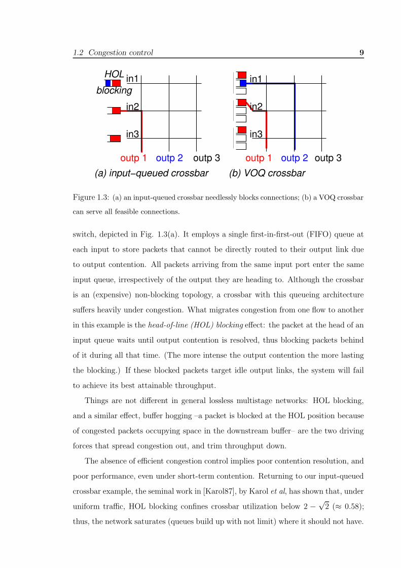
source 4 to destination B), receive poor service, as if they were congested. 71.3 (a) an input-queued crossbar needlessly blocks connections; (b) a VOQ
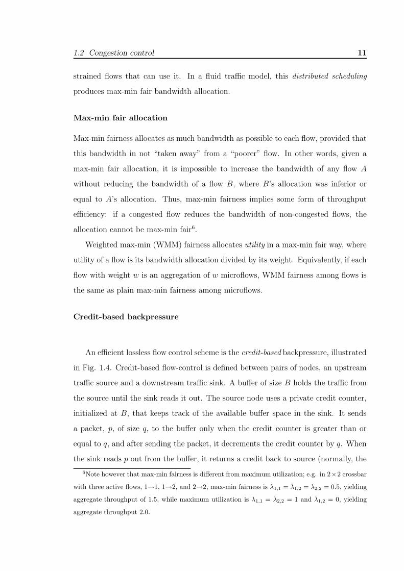
crossbar can serve all feasible connections. . . . . . . . . . . . . . . . . . 91.4 Illustration of credit-based flow control. The one way propagation delay
equals 2 packet times, and the round-trip time equals 4 packet times. As
shown in the figure, if the sink starts suddenly to read from a full buffer, the
first new data to arrive into the buffer will delay for one round-trip time;
thus, queue underflow will be avoided only if the filled queue length is ≥one round-trip time worth of data. . . . . . . . . . . . . . . . . . . . . . 12
1.5 The output queueing architecture. . . . . . . . . . . . . . . . . . . . . . 141.6 An input (virtual-output) queued switch, with shared on-chip memory. Per-
output logical queues are implemented inside the shared-memory. The mul-
tiplexing (demultiplexing) operation frequently includes serial-to-parallel
(parallel-to-serial) conversions –i.e. datapath width changes–, that perform
the routing needed in order to write an incoming packet to a specific mem-
ory location (read that packet on the correct output). Even though this
organization may be seen as a three-stage switch, it is custom to consider
it single-stage. . . . . . . . . . . . . . . . . . . . . . . . . . . . . . . . 161.7 The combined-input-output-queueing (CIOQ) switch architecture. . . . . 181.8 (a) bufferless VOQ crossbar; (b) buffered VOQ crossbar. . . . . . . . . . 191.9 Two iterations in a typical iterative bufferless crossbar scheduler. All schedul-
ing operations occur sequentially. The final, after the second iteration,
match is not maximal; one additional iteration would match the two un-
matched ports. . . . . . . . . . . . . . . . . . . . . . . . . . . . . . . . 211.10 The operations in a buffered crossbar; in each cell time, input and output
schedulers operate in parallel. . . . . . . . . . . . . . . . . . . . . . . . 221.11 A non-blocking, three-stage, Clos/Benes fabric, with no speedup; N=1024;
m = n = 32. . . . . . . . . . . . . . . . . . . . . . . . . . . . . . . . . 251.12 1024 ports in a three-stage, Clos/Benes fabric, with buffered crossbar elements. 261.13 1024 ports in a three-stage, Clos/Benes fabric, with discriminate flow-control,
and per-destination flow merging. . . . . . . . . . . . . . . . . . . . . . 271.14 1024 ports in a three-stage, Clos/Benes fabric, with hierarchical credit-based
backpressure. . . . . . . . . . . . . . . . . . . . . . . . . . . . . . . . . 28
ix

2.1 (a) traditional credit-based flow-control needs N window buffers; (b) request-
grant backpressure using one (1) window buffer. . . . . . . . . . . . . . . 322.2 Data round-trip time, and request round-trip time. Between the successive
reservations of the same credit via grant 1, the scheduler serves requests
using the rest of credits that it has available. . . . . . . . . . . . . . . . 342.3 A fabric with shared queues, one in front of each internal or output-port
link; (a) uncoordinated packet injections suffer from filled queues, inter-stage
backpressure, and subsequently HOL blocking; (b) coordinating packet in-
jections so that all outstanding packets fit into output buffers obviates the
need for inter-stage backpressure and prevents HOL blocking. . . . . . . . 372.4 Request-grant congestion control in a three-stage network. . . . . . . . . 382.5 The exact matches needed in bufferless fabrics versus the approximate matches
in buffered fabrics. . . . . . . . . . . . . . . . . . . . . . . . . . . . . . 392.6 A three-stage network using (a) discriminative backpressure, and (b) end-
to-end credit-based backpressure. . . . . . . . . . . . . . . . . . . . . . 402.7 Scheduling in bufferless three-stage Clos networks. . . . . . . . . . . . . . 50
3.1 Placement of buffers in a crossbar. Starting from the left, we have a buffer-
less crossbar, then a (buffered) crossbar containing a N -cell buffer per out-
put, and, last, on the right, a system with a 2-cell buffers per output. In
this chapter, we consider the latter type of switches (or fabrics), buffered
with less than N cell buffers per output. . . . . . . . . . . . . . . . . . . 543.2 A switch with small output queues managed using request-grant scheduled
backpressure. . . . . . . . . . . . . . . . . . . . . . . . . . . . . . . . . 563.3 The scheduling subsystem for a 4 × 4 VOQ switch with small, shared out-
put queues; the per-output (credit) schedulers and per-input (grant) sched-
ulers form a 2-stage pipeline, with the request and grant counters acting as
pipeline registers. . . . . . . . . . . . . . . . . . . . . . . . . . . . . . . 593.4 (a) when B= 1 (similar to bufferless crossbars), schedulers deterministically
desynchronize and achieve 100% throughput; (b) when B= N (similar to
buffered crossbars), 100% thoughput is achieved even when schedulers are
fully synchronized. . . . . . . . . . . . . . . . . . . . . . . . . . . . . . 613.5 100× (1− 1
N )(N ·B). . . . . . . . . . . . . . . . . . . . . . . . . . . . . . 623.6 Performance for varying buffer size, B; N= 32, P= 0, Rc= 1, and SD=1;
Uniformly-destined Bernoulli cell arrivals. Only the queueing delay is shown,
excluding all fixed scheduling and propagation delays. . . . . . . . . . . . 663.7 Performance for varying credit scheduler rate, Rc; N= 32, P= 0, SD= 1,
and B= 4; Uniformly-destined Bernoulli cell arrivals. Only queueing delay
is shown, excluding all other fixed delays. . . . . . . . . . . . . . . . . . 673.8 Performance for varying sw. size, N ; P= 0, Rc= 1, and SD= 1; Uniformly-
destined Bernoulli cell arrivals. Only queueing delay is shown, excluding all
other fixed delays. . . . . . . . . . . . . . . . . . . . . . . . . . . . . . 683.9 Performance for varying scheduling delay SD, and varying buffer size B; N=
32, P=0, Rc= 1; Uniformly-destined Bernoulli cell arrivals. Only queueing
delay is shown, excluding all other fixed delays. . . . . . . . . . . . . . . 69
3.10 Performance for varying scheduling delay SD, and varying P , with, and
without, credit prediction; N= 32, Rc= 1; Uniformly-destined Bernoulli
cell arrivals. Only queueing delay is shown, excluding all other fixed delays. 703.11 Throughput performance under unbalanced traffic for varying buffer size,
B; N= 32, P= 0, Rc= 1, and SD=1; full input load. . . . . . . . . . . . 713.12 Performance under bursty traffic, for different buffer sizes, B, when no grant
throttling is used; N= 32, P= 0, Rc= 1, and SD= 1 cell time; average burst
size 12 cells. Only queueing delay shown, excluding all other fixed delays. . 723.13 An unbalanced VOQs state, with input 2 being congested (bottlenecked):
(a) max-min fair rates; (b) credit issue rates versus credit return rates. . . 743.14 Due to the rate mismatch in Fig. 3.13(b), (a) credits accumulate in front
of congested input 2; (b) service rates when using threshold grant throttling. 753.15 Performance under bursty traffic, for different grant throttling thresholds,
TH; N= 32, B= 12; average burst size 12 cells; Only the queueing delay is
shown, excluding all other fixed delays. . . . . . . . . . . . . . . . . . . 773.16 Evolution of combined grant queue size (GQ) in front of individual inputs,
while simulating a 32×32 switch, with B= 12 cells and TH= 7, under
uniformly-destined, Bernoulli traffic at 100% input load. . . . . . . . . . . 793.17 How common-order round-robin credit schedulers, assisted by threshold
grant throttling, synchronize. Assume all inputs have request pending for
all outputs, and that TH= 2. Outputs are completely desynchronized in
the beginning of cell time 1, and one would expect them to remain desyn-
chronized thereafter. The figure shows what will happen if inputs 2 and 3
are Off in cell time 1, and turn On again in the beginning of cell time 2. . 803.18 Possible round-robin scan orders for random-shuffle output credit sched-
ulers. In a 3×3 switch, orders (a), (b), and (c) could correspond to outputs
1, 2, and 3, respectively. . . . . . . . . . . . . . . . . . . . . . . . . . . 823.19 Throughput performance under unbalanced traffic for varying buffer size, B,
and varying threshold values, TH, using common-order round-robin credit
scheduling; N= 32; Bernoulli arrivals. . . . . . . . . . . . . . . . . . . . 843.20 Throughput performance under unbalanced traffic for varying threshold,
TH, under different credit scheduling disciplines; B= 12 cells; all switches
have 32 ports, except one, 256-port clocks-TH5; Bernoulli arrivals. . . . . 853.21 Delay performance under varying average burst size (abs), for OQ, iSLIP
with 4 iterations, buffered crossbar with 1-cell crosspoint buffers, and for
the small buffers switch, with B= 12, TH= 5, and desynchronized clocks
credit schedulers; N= 32; Only the queueing delay is shown, excluding all
other fixed delays. . . . . . . . . . . . . . . . . . . . . . . . . . . . . . 863.22 Delay performance under varying average burst size (abs), for the small
buffers switch, with B= 12, TH= 5, and random-shuffle credit schedulers;
N= 32 and N= 256; Only the queueing delay is shown, excluding all other
fixed delays. . . . . . . . . . . . . . . . . . . . . . . . . . . . . . . . . 873.23 Performance under diagonal traffic for OQ, iSLIP with 4 iterations, buffered
crossbar with 1-cell crosspoint buffers, and for the small buffers switch, with
B= 12, TH= 5; N= 32; Bernoulli arrivals; Only the queueing delay is
shown, excluding all other fixed delays. . . . . . . . . . . . . . . . . . . 88

4.1 Multipath vs. static routing. . . . . . . . . . . . . . . . . . . . . . . . . 914.2 Pipelined buffer scheduling in a 4 × 4 (N= 4, M =2), three-stage, non-
blocking fabric. . . . . . . . . . . . . . . . . . . . . . . . . . . . . . . . 944.3 Simplified fabric scheduler for non-blocking networks. . . . . . . . . . . . 974.4 The in-order credits method that bounds the size of the reorder buffers.
Only credits of in-order cells are returned to the central scheduler. . . . . 100
5.1 (a) credit schedulers distributed inside the fabric, each one close to its cor-
responding output; (b) all credit schedulers in a central control chip. . . . 1025.2 An 1024×1024 three-stage, Clos/Benes fabric with buffered crossbar switch-
ing elements and a central control system. . . . . . . . . . . . . . . . . . 1045.3 An 1024×1024 three-stage, Clos/Benes fabric with central control; linecards
are not shown. . . . . . . . . . . . . . . . . . . . . . . . . . . . . . . . 1055.4 (a) fields of request/grant messages issued to and by the central scheduler,
before optimization; (b) fields of credits returned to the central scheduler,
before optimization. The width of the size field depends on the granularity
of buffer space reservations. In section 5.2.5 we remove the size field from
all messages; in section 5.2.4 we remove the route field from request/grant
messages; and in section 5.3.1 we remove the input field from request/grant
messages, and the output field from credit messages. . . . . . . . . . . . 1075.5 Datapath of a 4 × 4 fabric. Credits are sent upstream at the rate of one
credit per minimum-segment time, and convey the exact size of the buffer
space released, measured in bytes. . . . . . . . . . . . . . . . . . . . . . 1125.6 The egress linecard contains per-flow queues, in order to perform segment
resequencing and packet reassembly. . . . . . . . . . . . . . . . . . . . . 1135.7 The control (data) round-trip time; the delay of each scheduling operation
is one MinP -time. . . . . . . . . . . . . . . . . . . . . . . . . . . . . . 1145.8 Request-grant communication with the central scheduler using time di-
vision multiplexing (TDM). A single physical linecard serves both ingress
and egress functions; in the ingress path each linecard has an outgoing con-
nection to an A-switch; in the egress path, each linecard has an incoming
connection from a C-switch. . . . . . . . . . . . . . . . . . . . . . . . . 1155.9 The internal organization of the central scheduler for N= 4 and M= 2.
There are N 2 request counters, and N 2 grant counters. Not shown in the
figure are the N 2 flow distribution pointers and the N ·M credit counters. 1165.10 Throughput under unbalanced traffic; fixed-size cell Bernoulli arrivals; 100%
input load. (a) 64-port fabric (N= 64, M= 8); (b) varying fabric sizes up
to N= 256, M= 16. . . . . . . . . . . . . . . . . . . . . . . . . . . . . 1195.11 Delay versus input load, for varying fabric sizes, N ; buffer size b= 12 cells,
RTT= 12 cell times. Uniformly-destined fixed-size cell Bernoulli arrivals.
Only the queueing delay is shown, excluding all other fixed delays. . . . . 1205.12 Delay of well-behaved flows in the presence of hotspots. h/• specifies the
number of hotspots, e.g., h/4 corresponds to four hotspots. Fixed-size cell
Bernoulli arrivals; 64-port fabric, b= 12 cells, RTT= 12 cell times. Only the
queueing delay is shown, excluding all other fixed delays. . . . . . . . . . 121

5.13 Delay versus input load, for varying fabric sizes, N ; buffer size, b= 12 cells,
RTT= 12 cell times. Uniformly-destined bursty traffic with average burst
size equal to 12 cells. Only the queueing delay is shown, excluding all other
fixed delays. . . . . . . . . . . . . . . . . . . . . . . . . . . . . . . . . 1225.14 Delay versus input load; 256-port fabric, buffer size, b= 12 cells, RTT= 12
cell times; TH= 7. Uniformly-destined bursty traffic. Only the queueing
delay is shown, excluding all other fixed delays. . . . . . . . . . . . . . . 1235.15 Delay of well-behaved flows in the presence of hotspots, for varying bursti-
ness factors. Bursty fixed-size cell arrivals; 256-port fabric, b= 12 cells,
RTT= 12 cell times. Only the queueing delay is shown, excluding all other
fixed delays. . . . . . . . . . . . . . . . . . . . . . . . . . . . . . . . . 1245.16 Sophisticated output bandwidth allocation, using WRR/WFQ credit sched-
ulers; 64-port fabric, b= 12 cells, RTT=12 cell times. . . . . . . . . . . . 1255.17 Weighted max-min fair allocation of input and output port bandwidth, using
WRR/WFQ schedulers; 4-port fabric, b= 12 cells, RTT=12 cell times. . . 1275.18 Packet delay performance under variable-size packet arrivals, using variable-
size, multi-packet segments; Poisson packet arrivals on 10 Gb/s lines; uniform-
destined traffic; 64-port fabric. The SF delay includes the request-grant de-
lay, segment propagation through the fabric, as well as segment reordering
and packet reassembly delays. . . . . . . . . . . . . . . . . . . . . . . . 1295.19 Packet delay performance under variable-size packet arrivals, using variable-
size multi-packet segments; Poisson packet arrivals on 10 Gb/s lines; diag-
onal traffic distribution; 64-port fabric. The SF delay includes the request-
grant delay, segment propagation through the fabric, as well as segment
reordering and packet reassembly delays. . . . . . . . . . . . . . . . . . . 1305.20 Packet delay performance under variable-size packet arrivals, using variable-
size, multi-packet segments; Poisson packet arrivals on 10 Gb/s lines; uni-
form and hotspot destination distributions; uniform packet size; 64-port
fabric. The SF delay includes the request-grant delay, segment propagation
through the fabric, as well as segment reordering and packet reassembly
delays. . . . . . . . . . . . . . . . . . . . . . . . . . . . . . . . . . . . 1315.21 Per-stage fabric delays for (a) uniformly-destined traffic / uniform packet
size; (b) uniformly-destined traffic / bimodal packet size; and (c) 8-hotspot
traffic / uniform packet size; 64-port fabric. In (c), we only plot the delay
of the non-congested flows. . . . . . . . . . . . . . . . . . . . . . . . . . 1315.22 Throughput of SF under Poisson, variable-size packet arrivals, using variable-
size, multi-packet segments; unbalanced traffic distribution; 64-port fabric;
100% input load. . . . . . . . . . . . . . . . . . . . . . . . . . . . . . . 1325.23 Throughput of SF with crosspoint buffer size smaller than one RTT worth
of traffic; unbalanced traffic distribution; fixed-size cell Bernoulli arrivals;
256-port fabric, RTT= 64 cell times; 100% input load. . . . . . . . . . . . 1345.24 Delay of SF with crosspoint buffer size smaller than one RTT worth of
traffic; uniformly-destined traffic; 256-port fabric, RTT= 64 cell times; no
grant throttling used. Only the queueing delay is shown, excluding all other
fixed delays. . . . . . . . . . . . . . . . . . . . . . . . . . . . . . . . . 136
6.1 An 8×8, three-stage, output-buffered, banyan network, made of 2×2 switches.138

6.2 (a) Flows 1 and 2 are bottlenecked at link A-B; (b) before reserving any
buffers, the requests from these flows need to pass through the (oversub-
scribed) request link A-B, which slows them down at a feasible for link A-B
rate (the excess requests are held in per-flow request counters); (c) conse-
quently, the request from these flows that reach the credit scheduling unit
can be served fast. . . . . . . . . . . . . . . . . . . . . . . . . . . . . . 1406.3 The request and grant channels for a three-stage, 8 × 8 banyan network
made of 2× 2 switches. . . . . . . . . . . . . . . . . . . . . . . . . . . . 1426.4 The credit schedulers along the scheduling path of flows 1→1 and 1→2,
in an 8 × 8 banyan network; credit schedulers C1-B1 and B1-A1 reside in
switch B1; credit scheduler A1-Inp1 resides in switch A1. . . . . . . . . . 1436.5 Delay of well-behaved flows in the presence of hotspots. h/• specifies the
number of hotspots, e.g., h/4 corresponds to four hotspots. Bernoulli fixed-
size cell arrivals; N= 125 (M= 5), b= 12 cells, RTT= 12 cell times. Only
the queueing delay is shown, excluding all other fixed delays. . . . . . . . 1466.6 Delay of flow 1→3 when flow 5→2 is active (link B1-C1 saturated), and
when it is not (no internal link saturated). Bernoulli fixed-size cell arrivals;
8-port fabric, b= 12 cells, RTT= 12 cell times. Only the queueing delay is
shown, excluding all other fixed delays. . . . . . . . . . . . . . . . . . . 1476.7 Delay of flow 5→1 when flow 1→3 is active (link A1-B1 saturated), and
when it is not (no internal contention). Bernoulli fixed-size cell arrivals;
8-port fabric, b= 12 cells, RTT= 12 cell times. Only the queueing delay is
shown, excluding all other fixed delays. . . . . . . . . . . . . . . . . . . 148
7.1 The central scheduler of chapter 3 modified for buffered crossbar switches. 1507.2 A 3×3, buffered crossbar switch (a) with the input schedulers distributed in-
side the N ingress linecards; (b) with all input schedulers inside the crossbar
chip. . . . . . . . . . . . . . . . . . . . . . . . . . . . . . . . . . . . . 1527.3 The schedulers needed for credit prediction in buffered crossbars; the input
schedulers reserve crosspoint buffer credits as in Fig. 7.2(b); the virtual
output schedulers “predict” the release of credits. . . . . . . . . . . . . . 1557.4 Scheduling flow 1→1 in a buffered crossbar employing credit prediction; P=
2 cell times, B= 2 cells; with dark gray we mark input scheduling operations
that reserve the “same credit”, α. . . . . . . . . . . . . . . . . . . . . . 1577.5 Scheduling flow 1→1 in a traditional buffered crossbar; P= 2 cell times, B=
2 cells; with dark gray we mark input scheduling operations that reserve the
“same credit”, α. . . . . . . . . . . . . . . . . . . . . . . . . . . . . . . 1587.6 Performance for N= 32, P=0, D= 1/2 cell times, and B= 1 cell; Uniformly-
destined, Bernoulli and bursty (abs= 12 cells) cell arrivals; Only the queue-
ing delay is shown, excluding all fixed scheduling delays. . . . . . . . . . 1617.7 Throughput performance for varying rtt under unbalanced traffic; B= 2
cells; full input load. (a) traditional buffered crossbar; (b) buffered crossbar
employing credit prediction. . . . . . . . . . . . . . . . . . . . . . . . . 1627.8 Throughput performance for varying rtt under unbalanced traffic; in each
plot, B equals one rtt worth of traffic. (a) traditional buffered crossbar; (b)
buffered crossbar employing credit prediction. . . . . . . . . . . . . . . . 163

7.9 Scheduling flows 1→1 and 2→1 in a buffered crossbar employing credit
prediction; we assume that both request counters 1→1 and 2→1 are non-
zero from the beginning of cell time 1; P= 2 cell times, B= 2 cells. . . . . 165
A.1 A single path in the request and in the grant channel of the proposed dis-
tributed scheduler for three-stage Clos/Benes fabrics (N=4, M=2). . . . . 190A.2 Request and grant messages convey only the ID of the respective flow; the
information needed to identify a flow changes along the route of request-
grant messages. . . . . . . . . . . . . . . . . . . . . . . . . . . . . . . . 193A.3 Delay of well-behaved flows in the presence of hotspots; h/• specifies the
number of hotspots, e.g. h/4 corresponds to four hotspots. Fixed-size cell
Bernoulli arrivals; 64-port fabric, b= 12 cells, RTT= 12 cell times. Only the
queueing delay is shown, excluding all other fixed delays. . . . . . . . . . 195A.4 Delay of well-behaved flows in the presence of hotspots. Rate of B→C
request links equal to λc (1 requests / cell time, per link); 64-port fabric.
Hotspots are the outputs of switch C1. Fixed-size cell Bernoulli arrivals; b=
12 cells, RTT= 12 cell times. Only the queueing delay is shown, excluding
all other fixed delays. For some of the delays shown we have not achieved
the desired confidence intervals. . . . . . . . . . . . . . . . . . . . . . . 197A.5 Delay of well-behaved flows in the presence of hotspots. Rate of B→C
request links equal to 1.1·λc (1.1 requests / cell time, per link); 64-port
fabric. Hotspots are the outputs of switch C1. Fixed-size cell Bernoulli
arrivals; b= 12 cells, RTT= 12 cell times. Only the queueing delay is shown,
excluding all other fixed delays. . . . . . . . . . . . . . . . . . . . . . . 198


List of Tables
1.1 Complexity of the submodules of the switch [Katevenis04]. . . . . . 23
5.1 Packet size distributions. . . . . . . . . . . . . . . . . . . . . . . . . 128
xvii


Chapter 1
Introduction
The paradigm of digital computers –which encompasses processing, storage,
and retrieval of information– has gradually shifted during the last decades
from standalone, centralized systems, to distributed organizations built around an
interconnection network. The basic function of the interconnection network is to sup-
port the communication among otherwise isolated digital components. During the
90’s, interconnection networks have assumed a distinctive role of their own, through
the globalization of World-Wide-Web (WWW), and recently the emergence of peer-
to-peer systems. Within these digital, social networks, people, institutions, and pro-
grams from all over the world communicate with each other, full time and full range,
in selective or broadcast, exchange or sharing circumstances.
Switches are increasingly used to build the core of Internet routers, SAN cluster
and server interconnects, other bus-replacement devices, etc. The desire for scalable
systems implies a demand for switches with ever-increasing radices (port counts).
Beyond 32 or 64 ports, single-stage crossbar switches are quite expensive, and multi-
stage interconnection networks (switching fabrics) become preferable; they are made
of smaller-radix switching elements, where each such element is usually a crossbar.
It has been a longstanding objective of designers to come up with an economic in-
terconnection architecture, scaling to large port-counts, and achieving sophisticated
quality-of-service (QoS) guarantees under unfavorable traffic patterns. This thesis
addresses that challenge.
1

2 Chapter 1 Introduction
1
N
2
N
1
2
inpu
t−po
rtsinterconnectionnetwork (fabric)
contention
outp
ut−p
orts
Figure 1.1: N ×N interconnection network (fabric).
An abstract model of a N × N fabric is depicted in Fig. 1.1. There are a to-
tal of 2 · N ports, N of them serving as inputs (sources), and N of them serving
as outputs (destinations); all ports have the same bandwidth capacity (speed)1. In-
coming packets define the output-port(s) they are heading to, and the basic role of
the fabric is to forward them there as soon as possible, or, in general, according to
predefined quality-of-service (QoS) requirements. In this thesis we consider lossless
fabrics, which do not drop packets between fabric-input and fabric-output ports.
Fabric performance is often severely hurt by inappropriate decisions on how to
share scarce resources. Output contention is a primary source of such difficulties:
input ports, unaware of each other’s decisions, may inject traffic for specific outputs
that exceeds those outputs’ capacities. The excess packets must either be dropped,
thus leading to poor performance (lossy fabrics), or must wait in buffers (lossless
fabrics); buffers filled in this way may prevent other packets from moving toward
their destinations, again leading to poor performance. Tolerating output contention
in the short term, and coordinating the decisions of input ports so as to avoid output
1This model is quite general: if the numbers of inputs and outputs differ, imagine that some
of the N inputs are idle, or no packets are destined to some of the outputs; if port speed differs,
imagine that the rate of traffic injections never exceeds a given limit, or imagine that backpressure
(flow control) nevers allows the rate at some outputs to exceed a given limit.

1.1 Contents & contribution 3
contention in the long run is a complex scheduling problem, which cannot easily be
solved in a distributed manner; flow control and congestion management are aspects
of that endeavor. This thesis contributes to solving that problem.
1.1 Contents & contribution
This dissertation is structured as follows. The present chapter 1 is a general in-
troduction, describing fundamental ideas and tools, such as congestion, head-of-line
(HOL) blocking, per-flow queueing, flow merging, credit-based backpressure, hierar-
chical backpressure, etc. It also overviews alternative architectures for single-stage
switches, with emphasis given on bufferless and buffered crossbars and their schedul-
ing function. Chapter 1 concludes with an attempt to design a low-cost, three-stage
buffered fabric, with 1024 ports, using these present state-of-the-art methods, which
demonstrates the excessive cost that such a system would have.
Chapter 2 describes the key concepts of the contributions of this thesis. In particu-
lar, it describes the basic request-grant scheduled backpressure protocol, and outlines
how it can be deployed for congestion management in buffered multistage networks.
The new scheme utilizes a request-grant scheduling network, as many contemporary
bufferless networks do, but its operation is remarkably simpler, since, in a buffered
network, scheduling needs not be exact; effectively, the scheduling unit comprises
multiple, independent single-resource schedulers, that operate in parallel, and in a
pipeline. The role of the scheduling network is not to eliminate link conflicts, but to
confine their extent so as to secure well-behaved flows from congested ones. This is
accomplished by requesting and reserving buffer space in one or more buffers before
injecting the data into the network. What request-grant scheduled backpressure es-
sentially achieves is to shift the congestion avoidance burden from the data network
to the scheduling network, where it is much easier to handle “flooding requests”, as
requests have significantly smaller size than the actual data, and can be combined in
per-flow request counters. Chapter 2 also reviews prior & related work, and compares
it to our contribution.

4 Chapter 1 Introduction
In chapter 3, we apply request-grant scheduled backpressure to a single-stage
switch, with small, shared output queues. This single-stage setting serves as a sim-
plified model that allows for an in depth study of the request-grant scheduled back-
pressure. We also propose credit prediction, a scheme that makes output queue size
independent of the number of cells in transit between the linecards and the fabric.
In principle, buffer storage for only a few cells suffices for the fabric to reach high
performance: with 12 cells of buffer space per output, performance is better than in
buffered crossbars, which consume a buffer space for N (multiplied by a large control-
induced constant) cells per output! We study how transient input contention reduces
scheduling performance, by allowing buffer-credit accumulations, and we propose to
throttle the grants issued to bottleneck inputs. Finally, we discuss an intricate syn-
chronization phenomenon that shows up when all output schedulers visit inputs using
the same round-robin order; we alter these orders so as to avoid synchronization.
In chapter 4, we proceed to the multistage case. We first describe a generic
scheduling architecture, based on request-grant scheduled backpressure, that elim-
inates congestion in three-stage Benes fabrics; then, we simplify the scheduler by
capitalizing on the non-blocking property of Benes under multipath routing. Besides
congestion elimination, the scheduler can guarantee 100 percent in-order delivery us-
ing very small reorder buffers that can easily fit in on-chip memory.
Chapter 5 describes the organization of a 1024x1024, three-stage, non-blocking
Clos/Benes fabric, running with no internal speedup, made of 96 single-chip 32x32
buffered crossbar switching elements (3 stages of 32 switch chips each). This fab-
ric uses the scheduling methods proposed in chapter 4. We demonstrate that it is
feasible to place all the scheduling (control) circuity, centrally, in a single chip. The
proposed system can directly operate on variable-size packets, eliminating the padding
overhead and the associated internal speedup. Simulation results indicate very good
delay performance, and throughput that exceeds 95% under unbalanced traffic. Most
prominent is the result that, under hotspot traffic, with almost all output ports being
congested, flows destined to non-congested outputs experience negligible delay degra-
dation. In appendix A, we distribute the subunits of the scheduler inside the Benes

1.2 Congestion control 5
elements. A difficulty encountered pertains to the quadratic –due to multipath re-
quest routing– number of flows whose requests pass through each one of the switches
in the middle-stage of the network; effectively, we are forced to merge requests from
different flows. We use simulations to show that this decentralized (and thus even
more scalable) system also eliminates congested behavior.
In chapter 6, we consider some blocking network topologies, like the banyan. In a
banyan network, congestion management is even more difficult than in Benes, since,
besides output ports, internal links can cause congestion as well. We propose a fully
distributed scheduler for this network, comprising pipelined, single-resource sched-
ulers, that eliminates congestion from both internal and output-port links. The
scheduling network uses O(N) per-flow counters inside each switching element.
Chapter 7 applies credit prediction, a method that becomes feasible in conjuction
with request-grant scheduled backpressure (as proposed in chapter 3), to buffered
crossbar switches. Despite IC technology improvements, the on-chip memory in
buffered crossbars is yet a hard constraint, and the large round-trip time between the
fabric and the linecards would in principle imply a significant size for these memories.
Using credit prediction, the dependence of the crosspoint buffer size from this large
round-trip time is removed; effectively, crosspoint buffers can be made as small as
two cells each, thus significantly reducing cost. Simulations are used to demonstrate
that these new buffered crossbars perform robustly.
Finally, chapter 8 concludes this dissertation with a look back upon the work that
has taken place, and with a discussion on how future work can extend the developed
material.
1.2 Congestion control
In old-style circuit-switched networks, considerable research was driven by the de-
mand for low-cost network topologies with no internal blocking (non-blocking topolo-
gies), capable to switch in parallel any possible combination of one-to-one, input-
output connections. Clos and Benes networks [Clos53, Benes64] are among the most

6 Chapter 1 Introduction
prominent results of that research. Nowadays, that packet switching has supervened
upon circuit switching, the blocking problem has assumed new flavors and continues
to constitute a deep concern.
1.2.1 Congestion: yet another way to block connections
In order to dynamically share network resources, packet-switched networks employ
statistical multiplexing. In turn, statistical multiplexing introduces link contention
(packet conflict), when two or more packets demand the same link at the same time.
Depending on its degree, contention can either be short-term, when the long-term
packet rate is feasible, or long-term, when the long-term packet rate is infeasible.
The latter situation is commonly referred to as congestion, and assumes one or more
congested2 links. The flows and the packets using these links are similarly referred
to as congested. The behavior of a congested packet-switched network bears resem-
blances with the behavior of a circuit-switched network with internal blocking: the
latter network may not be able to connect two idling ports, because another con-
nection occupies some internal link(s). In a similar way, a packet-switched network
may not be able to provide a high-throughput connection between two idling ports,
because packets from congested connections occupy some internal buffer(s).
The congestion problem, commonly found under the name of hotspot contention,
has been identified since the very start of packet-switched networks [Kleinrock80,
Pfisher85]. The problem does not concern that much the congested flows per se,
but rather the co-existence, in certain network areas, of congested and non-congested
flows. During link overload, as the demand exceeds the available capacity, we can-
not do much to help congested flows: no matter what, their delays grow with no
bound3. It is the disturbances that congested flows bear on non-congested ones that
brings about the undesired congestion phenomena. Simply put, increasing the de-
mand beyond the capacity of a link may trim down the aggregate network throughput
2or bottleneck, or overloaded, or oversubscribed, or saturated.3On the other hand, an appropriate conjuction of packet buffering and packet scheduling can lift
the pressure caused by short-term contention.

1.2 Congestion control 7
1
2
3
4
destinationsother B
C
A
treecongestion
ingr
ess
sour
ces
hotspot 1
Figure 1.2: Ingress sources 1 to 4 inject packets destined at hotspot destination, A, ef-
fectively forming a congestion tree. Packets that have to cross areas in that tree in order
to reach non-congested destinations, (for instance from source 4 to destination B), receive
poor service, as if they were congested.
(throughput collapse).
In lossless interconnection networks, congestion is more difficult to handle than
in lossy networks, since we cannot drop packets when we discover that they are
congested; instead, we need to hold them inside network buffers, and to use flow
control (backpressure) feedback in order to prevent buffer overflow. Consider the
example in figure 1.2. Ingress sources, unaware of each other’s decisions, inject packets
into the network destined to the same link A, at an aggregate rate that this link (the
“hotspot”) cannot sustain4. The excess packets, which are outstanding inside the
network, form a congestion tree, i.e. a network of filled queues, that spans from the
conflicting sources (leaves) to the hotspot (root). Congested packets first accumulate
inside the queue in front of the hotspot (root), but, afterwards, due to backpressure
feedback, they also pile up inside queues in non-congested areas (close the leaves)5;
the congested packets depart from these queues at a rate dictated by the limited
capacity of the hotspot link. Subsequently, non-congested packets (i.e. heading to
non-congested destinations) that are using these queues progress only as the filled-
4In the long run, backpressure throttles sources’ injection, making the new incoming load feasible,
but this happens only after queues have filled up.5Congested trees may also form or disappear in other ways –see [Garcia05]

8 Chapter 1 Introduction
queue-pipe drains the congested ones, as if they were also congested (congestion
expansion).
1.2.2 The role of congestion control
The main duty of congestion control is to sustain incessant packet motion (throughput
efficiency). It should be noted here that whether the network topology be blocking or
non-blocking, congestion control is needed in order to avoid unnecessary “blocking”,
caused by flow interference. Apart from that, a good congestion control should evenly
allocate resources among equally competing flows (fairness). When links are not
oversubscribed, all users can be satisfied, and fairness is trivially obtained. It is only
when user demand surpass the available capacity that fairness becomes important
[Kleinrock80].
In order to reduce cost, congestion management schemes have been proposed that
assume that only a few links will be overloaded at any time instance. This assumption
may indeed be valid for some applications, but cannot be true for all applications,
and at all times. If one output can become overloaded, is there someone to guarantee
that N/2 or even more outputs cannot? For example, assume that, in a N × N
network, each input randomly selects one output to talk to. The probability, p, that
an output is chosen by two or more inputs (in which case it becomes overloaded)
equals 1−P [ selected by no input ]−P [selected by one input ]. Simple combinatorics
yield that, as N tends to infinity, p → N · (1− 2/e) ≈ N · 1/4; in other words, N/4
outputs are requested to carry more load than they can. Hence, a full solution to
the congestion problem should serve well-behaved flows independent of the number
of congested outputs.
1.2.3 HOL blocking & buffer hogging: congestion intermedi-
ates
To make the discussion more concrete, consider the simple input-queued crossbar
1.2 Congestion control 9
outp 3outp 2outp 1
HOL in1
in2
in3
(a) input−queued crossbar (b) VOQ crossbar
blocking
outp 2outp 1
in1
in2
in3
outp 3
Figure 1.3: (a) an input-queued crossbar needlessly blocks connections; (b) a VOQ crossbar
can serve all feasible connections.
switch, depicted in Fig. 1.3(a). It employs a single first-in-first-out (FIFO) queue at
each input to store packets that cannot be directly routed to their output link due
to output contention. All packets arriving from the same input port enter the same
input queue, irrespectively of the output they are heading to. Although the crossbar
is an (expensive) non-blocking topology, a crossbar with this queueing architecture
suffers heavily under congestion. What migrates congestion from one flow to another
in this example is the head-of-line (HOL) blocking effect: the packet at the head of an
input queue waits until output contention is resolved, thus blocking packets behind
of it during all that time. (The more intense the output contention the more lasting
the blocking.) If these blocked packets target idle output links, the system will fail
to achieve its best attainable throughput.
Things are not different in general lossless multistage networks: HOL blocking,
and a similar effect, buffer hogging –a packet is blocked at the HOL position because
of congested packets occupying space in the downstream buffer– are the two driving
forces that spread congestion out, and trim throughput down.
The absence of efficient congestion control implies poor contention resolution, and
poor performance, even under short-term contention. Returning to our input-queued
crossbar example, the seminal work in [Karol87], by Karol et al, has shown that, under
uniform traffic, HOL blocking confines crossbar utilization below 2 −√
2 (≈ 0.58);
thus, the network saturates (queues build up with not limit) where it should not have.
10 Chapter 1 Introduction
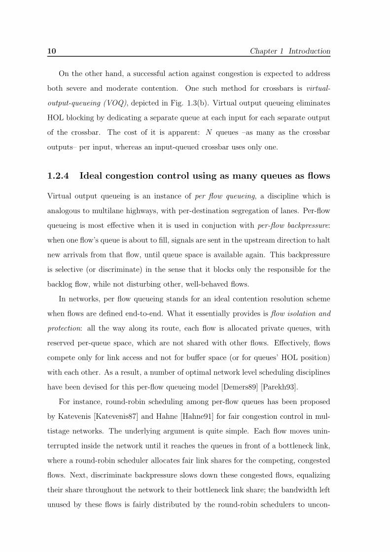
On the other hand, a successful action against congestion is expected to address
both severe and moderate contention. One such method for crossbars is virtual-
output-queueing (VOQ), depicted in Fig. 1.3(b). Virtual output queueing eliminates
HOL blocking by dedicating a separate queue at each input for each separate output
of the crossbar. The cost of it is apparent: N queues –as many as the crossbar
outputs– per input, whereas an input-queued crossbar uses only one.
1.2.4 Ideal congestion control using as many queues as flows
Virtual output queueing is an instance of per flow queueing, a discipline which is
analogous to multilane highways, with per-destination segregation of lanes. Per-flow
queueing is most effective when it is used in conjuction with per-flow backpressure:
when one flow’s queue is about to fill, signals are sent in the upstream direction to halt
new arrivals from that flow, until queue space is available again. This backpressure
is selective (or discriminate) in the sense that it blocks only the responsible for the
backlog flow, while not disturbing other, well-behaved flows.
In networks, per flow queueing stands for an ideal contention resolution scheme
when flows are defined end-to-end. What it essentially provides is flow isolation and
protection: all the way along its route, each flow is allocated private queues, with
reserved per-queue space, which are not shared with other flows. Effectively, flows
compete only for link access and not for buffer space (or for queues’ HOL position)
with each other. As a result, a number of optimal network level scheduling disciplines
have been devised for this per-flow queueing model [Demers89] [Parekh93].
For instance, round-robin scheduling among per-flow queues has been proposed
by Katevenis [Katevenis87] and Hahne [Hahne91] for fair congestion control in mul-
tistage networks. The underlying argument is quite simple. Each flow moves unin-
terrupted inside the network until it reaches the queues in front of a bottleneck link,
where a round-robin scheduler allocates fair link shares for the competing, congested
flows. Next, discriminate backpressure slows down these congested flows, equalizing
their share throughout the network to their bottleneck link share; the bandwidth left
unused by these flows is fairly distributed by the round-robin schedulers to uncon-
1.2 Congestion control 11
strained flows that can use it. In a fluid traffic model, this distributed scheduling
produces max-min fair bandwidth allocation.
Max-min fair allocation
Max-min fairness allocates as much bandwidth as possible to each flow, provided that
this bandwidth in not “taken away” from a “poorer” flow. In other words, given a
max-min fair allocation, it is impossible to increase the bandwidth of any flow A
without reducing the bandwidth of a flow B, where B’s allocation was inferior or
equal to A’s allocation. Thus, max-min fairness implies some form of throughput
efficiency: if a congested flow reduces the bandwidth of non-congested flows, the
allocation cannot be max-min fair6.
Weighted max-min (WMM) fairness allocates utility in a max-min fair way, where
utility of a flow is its bandwidth allocation divided by its weight. Equivalently, if each
flow with weight w is an aggregation of w microflows, WMM fairness among flows is
the same as plain max-min fairness among microflows.
Credit-based backpressure
An efficient lossless flow control scheme is the credit-based backpressure, illustrated
in Fig. 1.4. Credit-based flow-control is defined between pairs of nodes, an upstream
traffic source and a downstream traffic sink. A buffer of size B holds the traffic from
the source until the sink reads it out. The source node uses a private credit counter,
initialized at B, that keeps track of the available buffer space in the sink. It sends
a packet, p, of size q, to the buffer only when the credit counter is greater than or
equal to q, and after sending the packet, it decrements the credit counter by q. When
the sink reads p out from the buffer, it returns a credit back to source (normally, the
6Note however that max-min fairness is different from maximum utilization; e.g. in 2×2 crossbar
with three active flows, 1→1, 1→2, and 2→2, max-min fairness is λ1,1 = λ1,2 = λ2,2 = 0.5, yielding
aggregate throughput of 1.5, while maximum utilization is λ1,1 = λ2,2 = 1 and λ1,2 = 0, yielding
aggregate throughput 2.0.

12 Chapter 1 Introduction
credits cnt
credit
(0)
sourcesink buffer
one waypropagation del.=2 packet times
round−trip time
Figure 1.4: Illustration of credit-based flow control. The one way propagation delay equals
2 packet times, and the round-trip time equals 4 packet times. As shown in the figure, if the
sink starts suddenly to read from a full buffer, the first new data to arrive into the buffer
will delay for one round-trip time; thus, queue underflow will be avoided only if the filled
queue length is ≥ one round-trip time worth of data.
credit message contains the size q); upon receiving this credit, the source increases
the credit counter by q. To avoid deadlock, the buffer size B must be greater than or
equal to the maximum-packet-size.
The peak rate at which the source can write new data into the buffer is denoted
by λW , and the peak rate at which data are read out from the buffer is denoted by λR;
the corresponding average rates are denoted by λW and λR. Due to the conservation
law of bits, λR ≤ λW . Credit-based flow control enforces the reverse inequality,
effectively equalizing the steady write and read rates, i.e. λW = λR = λ. In order
to sustain the maximum steady rate (i.e. prevent queue underflow), the source must
be able to send a round-trip time7 (RTT ) worth of traffic before receiving a first
credit back. The traffic that worths this RTT equals RTT × λ?,, where λ? may be
computed either on steady rates, as λ, or on peak rates, as min(λW , λR), when the
former are unknown. In most cases, λW = λR = λ, and B ≥ RTT × λ; this product
is commonly referred to as one flow control (FC) window8. Observe that On/Off
7This round-trip time includes the propagation delay for the packet, and the propagation delay
for the credit (we assume that the queue implements cut-through, and we neglect interfacing and
queueing delays, as well as credit processing and packet scheduling times).8More accurately, for fixed-size packets, the flow control window is the integer multiple of the
packet size that equals or just exceeds RTT × λ; for variable-size packets, in [Katevenis04] we show
that the flow control window equals one maximum-size packet plus one RTT × λ.

1.3 Single-stage fabrics 13
backpressure (usually referred to as Stop&Go) requires at least twice that space. A
nice comparison between these two flow control schemes can be found in [Iliadis95].
1.2.5 No queueing, no congestion?
While per-flow queueing achieves excellent congestion management via extensive
buffering, at the other end of the spectrum, bufferless networks avoid congestion
in a rather straightforward manner: as no packet ever halts inside the fabric, con-
gestion trees cannot form, and the “road is always clear” for new connections. The
congestion-free property of bufferless networks comes however at the expense of ei-
ther (potentially heavy) packet loss, or, for lossless operation, at the expense of a far
too complicated central scheduler. Given the present demand at the network ingress
points, this scheduler’s duty is to identify sets of non-conflicting packets, and select
an effective one among them. This is a cumbersome task, given that it must be per-
formed in every new packet time, centrally, considering all link reservation and their
interdependencies in a single step.
Some bufferless networks, such as the Data Vortex switch [Yang00], obviate the
need of a central scheduler; instead, these networks use distributed control, and de-
flection lines inside the fabric, which misroute (or circulate) packets until the targeted
resource becomes available. However, these deflection lines form the equivalent of a
buffer, thus creating the conditions for congestion expansion [Chrysos04b] [Iliadis04].
1.3 Single-stage fabrics
Single-stage packet switches (fabrics) form the equivalent of a highway junction. Just
as with a junction connecting your home to the market square, “one turn and you are
there”, single-stage fabrics connect a small number of data ports by a single crosspoint.
Single-stage switches are not scalable, due to the quadratic cost of dedicating one
crosspoint for each input-output port pair. However, single-stage switches are easier
to comprehend and analyze than multistage fabrics, which comprise multiple single-
stage switches that operate in tandem and in parallel.

14 Chapter 1 Introduction
outputbuffer
outputbuffer
outputbuffer
Nx λ routing
λ
input 2
input 1
input N
output 1
output N
output 2
λ
Fabric
Figure 1.5: The output queueing architecture.
1.3.1 Routing and buffering
The most effective fabric that can possibly be built is the output queueing (OQ)
switch. In this ideal architecture, arriving packets are immediately stored in a buffer in
front of their output port –see Fig. 1.5. Output queueing performs best, as its internal
network does not impose any contention at all9. Effectively, packet delay depends
only on input demand and output capacity. Reference [Minkenberg01] proposes the
following definition:
A switch belongs to the class of output queueing if the buffering function is
after the routing function.
According to this description, many switches, such as the Knockout switch pro-
posed in the eighties [Yeh87], belong to the output queueing family. However, the
9To better appreciate the high quality of output queueing, consider one thousand people in their
houses, which, after watching a great advertized offer in the television, they all decide to go and
buy something from market store A. In a transportation model equivalent to output queueing, each
prospective customer, immediately after comprehending his/her need, will follow a private lane that
connects his/her house to an always available parking spot in front of store A. By contrast, in other
“switch architectures”, customers may first have to call in order to book parking area, go through
a pipe of junctions inside the city center, be delayed behind backlogs heading e.g. to a congested
public event, wait outside the filled parking lot, delay people that have an appointment with their
dentist, etc.

1.3 Single-stage fabrics 15
Knockout switch may drop packets inside the routing subsystem; by contrast, pure
(ideal) output queueing assumes perfect routing and infinite output buffers. Unfortu-
nately, it is not practical to build such switches due to memory bandwidth limitations:
each output queue must run N + 1 times faster than the line rate (λ), in order to
accommodate parallel packet arrivals from any number of up to N inputs, and, at
the same time, feed the outgoing link.
To alleviate the memory costs of output queueing, shared-memory switches are
used whenever this is feasible. These switches take advantage of the fact that the
combined write throughput to all output buffers cannot exceed N × λ (the aggregate
input rate). Thus, whereas pure output queueing uses N buffers of speed (N +1)×λ,
each, shared-memory uses a single buffer of speed 2×N × λ, which suffices to write
and read the aggregate input and output traffic, respectively.
In a shared-memory switch, the N output queues share buffer memory resources.
Sharing improves performance when some outputs are inactive, as the remaining
outputs can fully utilize the buffer space; however, sharing may also induce memory
monopolization (i.e. buffer hogging), wherein the queue of an output takes over most
of the memory space, preventing packets for other outputs from gaining access. This
bad aspect of buffer sharing led to schemes that bound the occupancy of individual
queues [Katevenis98] [Hahne98] [Minkenberg00].
Building a large buffer that accommodates the load of N links may be expensive,
because large buffers can only be implemented off-chip, and high off-chip bandwidth
requires many I/O pins and wide traces on PCBs10. This is the drawback of both
output-queueing and shared-memory. The memory bandwidth of a N × N switch
is most effectively tackled when the buffering function is distributed over N input
linecards, in front of the switching fabric. Memories at inputs need run only two
times faster than the line, and can be implemented using off-chip DRAMs. This is
how input queueing switches work. According to [Minkenberg01]:
A switch belongs to the class of input queueing if the buffering function is per-
10printed circuit boards, upon which chips are placed.

16 Chapter 1 Introduction
outp 1outp 2
outp NNλ Nλ
λ
Linecards
VOQs
VOQs
λ VOQsinp 1
inp N
inp 2
logicalqueues
on−chipshared−memory
mul
tiple
Fabric
λoutp 1
outp 2
outp N
dem
ultip
lexi
ng
Figure 1.6: An input (virtual-output) queued switch, with shared on-chip memory. Per-
output logical queues are implemented inside the shared-memory. The multiplexing (de-
multiplexing) operation frequently includes serial-to-parallel (parallel-to-serial) conversions
–i.e. datapath width changes–, that perform the routing needed in order to write an incom-
ing packet to a specific memory location (read that packet on the correct output). Even
though this organization may be seen as a three-stage switch, it is custom to consider it
single-stage.
formed before the routing function (switching).
The fabric of a single-stage, input queued switch can either be a bufferless crossbar,
or may contain small, on-chip buffers –see for instance Fig. 1.6, or Fig. 1.8(b). As
noted in section 1.2.3, input queues should be organized per-output (VOQ), in order
to eliminate HOL blocking11.
1.3.2 Bufferless crossbars vs. buffered crossbars
Based on experience gained during earlier stages of this research [Chrysos03a, Katevenis04],
we prefer buffered fabrics in this work. This earlier research demonstrated the ad-
11This especially holds for bufferless crossbars, which cannot tolerate any output contention at all
[Karol87]. It is interesting to note here that, as demonstrated in [Lin04], when traffic is smooth, a
buffered crossbar diminishes the effect of HOL blocking inside FIFO input queues: a packet at the
head of the FIFO will not be held back, even if other inputs are targeting the same output at the
same time, as long as crosspoint buffers are not full; instead, resolution of short-term conflicts can
take place inside the fabric, thus avoiding the HOL blocking behavior.

1.3 Single-stage fabrics 17
vantages of a buffered crossbar core over a bufferless one: scheduling simplicity and
efficiency.
Bufferless crossbars
The hardest part of a high-speed bufferless VOQ crossbar is the scheduler needed to
keep it busy. With VOQs at the input ports, the crossbar scheduler has to coordinate
the use of 2 × N interdependent resources. Each input has to choose among N
candidate VOQs, thus potentially affecting all N outputs; at the same time, each
output has to choose among potentially all N inputs, thus making all 2 · N port
schedulers depend on each other.
As shown by Anderson et al [Anderson94], crossbar scheduling can be formalized
as bipartite graph matching –see Fig. 1.9: create a 2N -node bipartite graph with N
input nodes on the left side, and N output nodes on the right side; match with an
edge each input node with only one output node, and vice versa. When scheduling
a crossbar, valid input-output edges are those that correspond to non-empty VOQs.
A matching has maximum size if the number of edges is maximized; a matching
has maximum weight if the sum of edge weights is maximized; and, a matching is
maximal if we cannot add a new edge to it without altering the already formed edges
[Marsan02]. McKeown et al [McKeown99b] prove that maximum weight matches
can achieve 100% throughput under any admissible traffic pattern and surpass both
maximum size and maximal matches; however, the required algorithms have O(N 3)
complexity, and cannot be implemented at high speed.
Practical architectures for high-speed crossbar scheduling use multiple iterations of
handshaking between input and output ports [Anderson94] [McKeown99a] [Serpanos00]
[YLi01], which result in or close to maximal matches. On average, log2 N scheduling
iterations are needed to obtain a maximal match, thus complexity and cost increases
significantly when the number of ports rises. These schedulers either ignore QoS
issues, or provide only static priorities and round-robin scheduling. Weighted round-
robin behavior is very hard to achieve while still maintaining high crossbar utilization
[Ni01]. In addition, existing crossbar schedulers assume that all changes in the cross-

18 Chapter 1 Introduction
outputbuffer
outputbuffer
λoutput 1
output 2
output N
s x λ s x λ
routingFabric
input 2
input N
Linecards
λinput 1 output
buffer
Linecards
VOQs
VOQs
VOQs
Figure 1.7: The combined-input-output-queueing (CIOQ) switch architecture.
bar schedule take place at the same time. For such synchronous operation to be
possible, variable-size packets need to be segmented into fixed-size cells before enter-
ing the crossbar. To cope with segmentation overhead, internal speedup is required12.
Effectively, the solution commonly used today to cope with scheduling inefficien-
cies and with packet segmentation is to provide significant internal speedup [Krishan99]:
the crossbar port rate is higher than line rate by a factor of s, considerably greater
than one. In the resulting combined-input-output-queueing (CIOQ) architecture,
packets pile up in queues in front of the external outputs, resembling the output
queueing architecture –see Fig. 1.7. Even though speedup is a good solution, it does
incur significant cost:
1. The lines in and out of the crossbar chip need to run s times faster. Crossbar
chip power consumption is often the limiting factor for aggregate throughput,
and power consumption directly and critically depends on I/O throughput. This
has as consequence that, with a speedup of three for example, the maximum
system throughput is one third of what we could reach without speedup.
2. The crossbar lines are more expensive (s times higher throughput). Also the
crossbar scheduler must find matches in 1/s of the time it would normally have
12For example, to handle a sequence of 65-byte back-to-back cells, a 64-byte-cell system needs a
speedup of 128/65 ≈ 2.

1.3 Single-stage fabrics 19
VOQB B B
VOQ
VOQ
VOQ
B B BVOQ
B B BVOQ
(a) (b)
Figure 1.8: (a) bufferless VOQ crossbar; (b) buffered VOQ crossbar.
available.
3. The buffer memories are more expensive ( (1 + s)/2 times higher throughput
), and their number is doubled: as the capacity of the crossbar core exceeds
the aggregate capacity of the external links, besides input VOQs, large (off-
chip) queues are needed at the egress side of the system as well, in order to
compensate for the rate mismatch.
Buffered crossbars
An alternative solution, with the potential to yield both faster and less expensive
switches, is to use buffered crossbars –combined-input-crosspoint-queueing (CICQ). By
adding even small amounts of buffer storage at the crosspoints (see Fig. 1.8(b)), the
scheduling problem changes radically and is dramatically simplified: the 2×N sched-
ulers, N at the inputs and N at the outputs, now work independently of each other,
since each of them deals with only a single resource. The 2 × N schedulers are still
coordinated but only over longer time-scales, through backpressure feedback from the
crosspoint buffers. Essentially, crosspoint buffering allows solving the bipartite graph
matching problem in an approximate and long-term way, rather than the exact and
short-term way needed in bufferless crossbars. The main benefit of buffered crossbars
is their efficient operation even when no internal speedup is used. Scheduler indepen-
dence in buffered crossbars removes the requirement for synchronization to a common

20 Chapter 1 Introduction
clock, hence variable-size packets (or variable-size segments) can directly be switched
through the buffered crossbar core eliminating the internal speedup needed for seg-
mentation overhead [Yoshigoe01] [Katevenis04] [Katevenis05]. Furthermore, unlike
their bufferless counterparts, buffered crossbars with no speedup achieve small delays
and high throughput13[Rojas-Cessa01] [Mhandi03] [Yoshigoe03]. Finally, thanks to
their per-flow buffers14, buffered crossbars are capable of weighted round-robin, or
strict priority, scheduling [Stephens98] [Chrysos03a] [Luijten03] [Chrysos04a].
Almost all the results reported in the aforementioned papers are based on simula-
tion experiments. Up to now, only a few analytical results consider buffered crossbars
with no speedup [Javidi01] [Georgakopoulos04a, Georgakopoulos04b]. Instead, there
is a growing body of analytical work [Magill03] [Iyer05] [Turner06] on buffered cross-
bars using considerable speedup, between 2 and 4.
Scheduling similarities and differences
The style of scheduling in buffered crossbars is similar with iterative schedulers
for bufferless crossbars. Both systems use 2 ·N subschedulers, one per crossbar port,
which all try to coordinate with each other.
The operation of a typical iterative bufferless crossbar scheduler is depicted in
Fig. 1.9. Consider that all operations shown must occur in every single cell time,
i.e. the time it takes to transmit a fixed-size cell on a link. Each scheduling cy-
cle consists of one or more iterations (two iterations in figure 1.9); each iteration
consists of a grant phase and an accept phase. In the first phase of each iteration,
each output, independently, grants one of the demanding inputs. Although output
schedulers operate independently in this phase, their final decisions are dependent.
After output scheduling, an input may receive grants from several outputs, but it can
accept only one of them. To affirm this constraint, in the second phase, each input,
independently, accepts one of the output grants issued for it. The accepted grants
13Multi-cell crosspoint buffers or sophisticated link schedulers can be used in order to improve
throughput performance under unbalanced traffic.14Flows here are defined by input-output pair of the crossbar –not network-wise end-to-end.

1.3 Single-stage fabrics 21
inputs outputs
inputs outputs
inputs outputs
S
S
inputs outputs
S
S
S
inputs outputs
inputs outputs
S
demand bipartite graph
S
ITE
RA
TIO
N 1
ITE
RA
TIO
N 2
dropped
output grant input accept
inputs outputs
inputs outputsmatching
injected cells
mat
ched
dropped
Figure 1.9: Two iterations in a typical iterative bufferless crossbar scheduler. All scheduling
operations occur sequentially. The final, after the second iteration, match is not maximal;
one additional iteration would match the two unmatched ports.
correspond to matched input-output pairs, and cells from the corresponding VOQs
can safely be injected into the crossbar. Output grants that are not accepted by their
inputs are dropped (discarded), thus wasting processing resources.
Consider what would happen if one such grant, g, produced by output o, were
stored rather than being dropped. If output o was not allowed to produce a new
grant before g got accepted by its input scheduler, then output o would have stayed
underutilized for all that time; on the other hand, if output o was allowed to produce
new grants, then it could have happened that more than one grants of the same output
were accepted concurrently by their (independent) input schedulers, thus violating
the output constraint of the bufferless crossbar. Thus, non-accepted grants must be
dropped; the next iteration(s) will try to serve the corresponding outputs. As link
rates increase, the cell time shrinks, and so does the time available for scheduling;
effectively, it becomes very difficult to implement multiple iterations.
The operation of a typical buffered crossbar is depicted in Fig. 1.10. In the
first phase, which in buffered crossbars may last for a complete cell time, each in-

22 Chapter 1 Introduction
inputsinputs outputs outputsS
S
S
inputs outputs
SS
S
S
credit
in crosspointswrite packets read packet
from crosspoints
cell time 1 cell time 3cell time 2demand graphinputs outputs
S
S
S
S
Figure 1.10: The operations in a buffered crossbar; in each cell time, input and output
schedulers operate in parallel.
put scheduler, independently, selects one output to send a cell to. Multiple input
schedulers may select the same output, but this is not a problem, since the forwarded
cells will be stored in the crosspoint buffers until their output scheduler reads them
out, one by one. As with bufferless crossbars, schedulers’ decisions may be conflicting
because schedulers operate independently. However, the difference in buffered cross-
bars is that schedulers are truly independent: no decision ever has to be cancelled
or revoked because of resource conflicts. This is a striking difference: in bufferless
crossbars, the matching procedure starts from scratch in every new cell time, and
the same conflicts may be repeated again and again, reducing switch throughput; in
buffered crossbars, conflicting packets are held in crosspoint buffers, and create the
conditions for matchings (output utilization) to become full shortly in the future.
1.3.3 Single-chip buffered crossbars
Although advantageous, the buffered crossbar architecture was not very popular in
high-end products, due to the difficulty, in the past, to integrate large amounts of
memory on the crossbar chip. With the progress of semiconductor technology, how-
ever, we are today at the point where buffer space of a few MBytes can be placed on
an ordinary chip; thus, buffered crossbars have attracted considerable interest from
industry and academia. From the industry side, IBM has designed a 64× 64 buffered
crossbar, at 40 Gbp/s per port [Abel03]. Because this large design requires excessive

1.3 Single-stage fabrics 23
Module Gates Flip-Flops SRAM Area Area Power Power
(number of (K) (K) 2-port 0.18µm 0.13µm 0.18µm 0.13µm
instances) (bits) (mm2) (mm2) (Watt) (Watt)
XPM (1024) 16 M 286.0 130.00 1.0 0.2
OS (32) 41.5 11.0 2.5 1.49 0.5 0.3
Wiring 117.7 60.94 3.6 2.2
Subtotal 41.5 11.0 16 M 405.5 192.43 5.1 2.7
Estimated power consumption of 32 link SERDES and pad drivers 23.040 14.400
Table 1.1: Complexity of the submodules of the switch [Katevenis04].
amounts of on-chip memory, the crossbar fabric is implemented in multiple chips that
operate in parallel using bit slicing. The switch architecture research team here at
FORTH has also been one of the first to identify and explore the benefits of buffered
crossbars. Our previous research considered cell-based buffered crossbars systems,
and their capability for weighted max-min fair scheduling [Chrysos02] [Chrysos03a].
Later on, the design of a single-chip, 32×32 buffered crossbar switch, at 10 Gbp/s per
port, which directly operates on variable-size packets, helped us better appreciate the
efficiency and the hardware simplicity of this architecture [Katevenis04] [Passas03]
[Simos04].
Table 1.1 depicts gate, flip-flop, SRAM, area and power consumption cost for this
32× 32 buffered crossbar chip [Katevenis04]. The lines refer to: crosspoint datapath
(XPD), crosspoint memory (XPM), and output scheduler (OS)15. Two KByte cross-
point buffers are implemented in order to support unsegmented packets of size up to
the usual IP size limit of 1500 bytes. As can be seen, everything else besides cross-
point memories and wiring occupies just 5% of the area, indicating the simplicity of
the architecture. The power consumption of the core (line subtotal) is a small fraction
of the power consumption estimated for the interfaces of the chip, which communi-
cate information with the ingress and egress linecards. The I/O portion of power
15The design implements credit-based backpressure from the crosspoint buffers to the ingress
linecards.

24 Chapter 1 Introduction
(SERDES and pad drivers) must be paid anyhow, whether the crossbar be buffered
or bufferless. Effectively, buffered crossbars, by obviating the need for speedup, can
support higher external capacities at a given cost level, or, equivalently, implement a
targeted capacity at lower cost.
1.4 Motivation
The research in this thesis is motived by the desire to scale interconnection systems to
ever larger port counts, beyond single-stage capabilities. We envision accommodating
1024 bidirectional ports in a three-stage, non-blocking Clos fabric as the first step in
this direction.
1.4.1 Non-blocking three-stage fabrics
Switching fabrics are said to present internal blocking when internal links do not
suffice to route any combination of feasible I/O rates, hence, long-term contention
may appear on internal links as well, in addition to output ports. Otherwise, a fab-
ric is called non-blocking when it can switch any set of flows that do not violate
the input and output port capacity limits16. Although internal blocking clearly re-
stricts performance, most commercial products belong to this first category, because a
practical, robust, and economic architecture for non-blocking fabrics has not been dis-
covered yet. However, neither has it been proven that such architectures do not exist.
This thesis contributes to the search for practical, robust, and economic non-blocking
switching fabrics.
Low-cost practical non-blocking fabrics are made using Clos networks [Kabacinski03];
the basic topology is a three-stage fabric, while recursive application of the principle
can yield 5- and more stage networks. One of the parameters of Clos networks, m/n,
controls the speed expansion ratio –something analogous to the “internal speedup”
used in combined input-output queueing (CIOQ) architectures: the number of middle-
16The crossbar is a non-blocking network, however its N 2 cost is prohibitively high for large N .

1.4 Motivation 25
1
2
1
2
32
32 32
CBA1
2
3232
1
1024
993
fabr
ic−i
nput
por
ts 1
993
1024 fabr
ic−o
utpu
t por
ts
Figure 1.11: A non-blocking, three-stage, Clos/Benes fabric, with no speedup; N=1024;
m = n = 32.
stage switches, m, may be greater than or equal to the number of input/output ports
per first/third-stage switch, n. In this thesis, we assume m = n, i.e. no speedup –the
aggregate throughput of the middle stage is no higher than the aggregate through-
put of the entire fabric. In this way, the fabrics considered here are the lowest-cost
practical non-blocking fabrics, oftentimes also referred to as Benes fabrics [Benes64].
1.4.2 A 1024-port, 10 Tbit/s fabric challenge
Figure 1.11 depicts a 1024×1024 Clos/Benes fabric (radix N=1024), made out of 96
single-chip 32×32 switching elements (3 stages of 32 switch chips of radix M= 32
each.) Not shown in the figure, and not included in the chip count, are the 1024
linecards. There are 1024 ingress/egress linecards, each one feeding one fabric input,
and being fed by one fabric output. In the ingress path, linecards terminate the
external incoming links, and contain VOQs where the main bulk of packet storage
takes place; in the egress path, linecards are responsible for packet resequencing and
forwarding packets to the external outgoing links. Packet reassembly, if needed, also
occurs here; however, the system that we design in this thesis is capable to directly
switch variable-size packets.
To define a full design, one has to describe the queueing organization of the switch-

26 Chapter 1 Introduction
cros
spoi
nt
cros
spoi
nt
cros
spoi
nt
A1 B1 C1out1
out2in1
in2 B2A2 C2B2
bkpr bkprbkprV
OQ
s
Figure 1.12: 1024 ports in a three-stage, Clos/Benes fabric, with buffered crossbar elements.
ing elements, and the scheduling architecture17. An important design challenge that
we took from the start of this project is to fit each switching element into a single chip.
Assuming that individual queue size (i.e. a FC window) ranges from a few hundred
bytes up to a few KBytes, we can implement a few thousands of such queues using
on-chip memory (e.g., 1024 queues, of 3 KBytes each), but not several thousands of
them (e.g., not 32K queues, since they would consume 256 Mbits of memory). Re-
placing 1024 by N , the pertaining constraint is that we cannot handle significantly
more than N queues inside any particular (single-chip) switch of the fabric.
In this setting, pure per-flow queueing is clearly infeasible, for the following reason.
Due to multipath routing, there are too many input-output pair flows to pass through
each link, and pure per-flow queueing allocates a separate queue for each one of them.
To see the cost of it, consider a flow, f , coming from fabric-input port 1 and heading
to fabric-output port 1. Multipath routing will steer the load of f across all links
going out of switch A1. Thus, per-flow queueing consumes M queues inside A1 for f
alone, and there are M ×N flows like f –from M A1-inputs to N fabric-outputs.
1.4.3 Why state-of-art fails
The first alternative we consider, shown in Fig. 1.12, employs M ×M buffered
crossbar switches in all switch stages. Without loss of generality, the figure assumes
17In the three-stage non-blocking network we consider, another central issue is the multipath
routing strategy, and the reordering method; we will address these issues later.
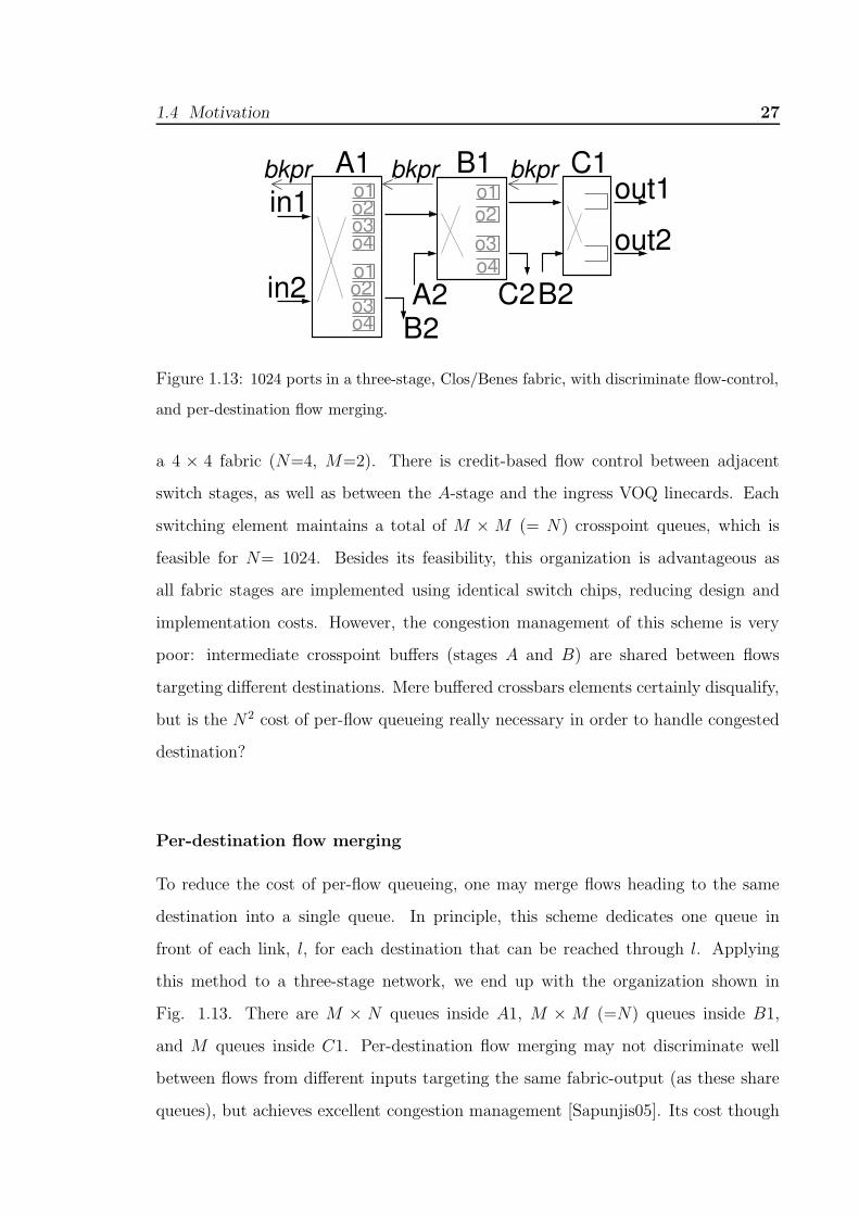
1.4 Motivation 27
B2A2 C2B2in2
in1 o2o1
o3o4
o2o1
o3o4
o1o2o3o4
bkpr bkprbkprout1
out2
C1B1A1
Figure 1.13: 1024 ports in a three-stage, Clos/Benes fabric, with discriminate flow-control,
and per-destination flow merging.
a 4 × 4 fabric (N=4, M=2). There is credit-based flow control between adjacent
switch stages, as well as between the A-stage and the ingress VOQ linecards. Each
switching element maintains a total of M × M (= N) crosspoint queues, which is
feasible for N= 1024. Besides its feasibility, this organization is advantageous as
all fabric stages are implemented using identical switch chips, reducing design and
implementation costs. However, the congestion management of this scheme is very
poor: intermediate crosspoint buffers (stages A and B) are shared between flows
targeting different destinations. Mere buffered crossbars elements certainly disqualify,
but is the N2 cost of per-flow queueing really necessary in order to handle congested
destination?
Per-destination flow merging
To reduce the cost of per-flow queueing, one may merge flows heading to the same
destination into a single queue. In principle, this scheme dedicates one queue in
front of each link, l, for each destination that can be reached through l. Applying
this method to a three-stage network, we end up with the organization shown in
Fig. 1.13. There are M × N queues inside A1, M × M (=N) queues inside B1,
and M queues inside C1. Per-destination flow merging may not discriminate well
between flows from different inputs targeting the same fabric-output (as these share
queues), but achieves excellent congestion management [Sapunjis05]. Its cost though

28 Chapter 1 Introduction
A1in1
in2B2A2
out1
out2
B1
C2B2
o1o2o3o4o1o2o3o4
cros
spoi
nt
C1A1A2
A2A1
bkprlevel−two backpr.
bkpr
Figure 1.14: 1024 ports in a three-stage, Clos/Benes fabric, with hierarchical credit-based
backpressure.
is prohibitive in the context of our “challenge”, at least within the current decade.
Besides the excessive number of queues inside A1, each queue must run at a speed of
M , in order to accommodate concurrent packet arrivals from any number of incoming
links. To alleviate this cost, one would have to partition each queue into M parts,
and associate each resulting sub-queue to a particular upstream. Doing so however
multiplies the number of queues per-switch by a factor of M 18.
Hierarchical credit-based backpressure
The approach depicted in Fig. 1.14 differs from the previous one in two fundamental
ways. First, we have moved the queues in switch A1 from the output side to the input
side. On the positive side, each queue is now associated with a particular upstream
linecard, and thus queue write speed equals line rate; on the negative side, A1 queues
are not anymore associated with switch outputs, thus a crossbar scheduler is needed
in A1.
Second, we have replaced the per-destination queues inside B1 with mere cross-
point queues. In conjuction, we consider a hierarchical credit-based flow control. Un-
der this protocol, A1 maintains private credits for a queue in front of every fabric-
18Remember that per-upstream partitioning of queues is mandatory under conventional credit-
based backpressure.

1.4 Motivation 29
output, and refrains from forwading any packets until such credits are available for
the targeted output. No backpressure is needed to control packet departures from
B-switches, as C-stage credits have already been reserved for these packets. Effec-
tively, congestion can not migrate to well-behaved flows, even if these flows share the
crosspoint queues in the second stage with congested ones: since backpressure from
the C-stage is not present, the shared crosspoint queues drain at peak rate, and thus
no HOL blocking develops in them19. As shown in Fig. 1.14, this scheme dedicates
one queue in front of each fabric-output port for every A-switch, for a total of M×M
(=N) queues per C-switch, which is feasible for N= 1024. Unfortunately, the C-stage
queues can be concurrently written by any number of B-switches, while partitioning
each one of them into M sub-queues that operate at the line rate exceeds our memory
constraint.
Observe that modifying the above hierarchical scheme so as to control packet
departures from the ingress stage, instead from the A-stage, obviates the need of
per-flow queues inside both A and B stages. However, this new scheme requires even
more queues: N queues in front of each fabric-output port, without per-B-switch
partitioning.
1.4.4 The need for new schemes to control traffic
The previous section showed that in order to protect flows from each other in a three-
stage non-blocking fabric with 1024 ports using current state-of-the-art methods, the
number of queues per switch, in at least one stage of the fabric, exceeds 32 K; un-
fortunately, traditional credit-based flow control, per-flow queueing, per-destination
flow merging, and hierarchical backpressure, do not get us to the goal that we set out
for.
Hence, new, innovative flow and congestion control methods must be devised to
19Note that, depending on the load distribution policy, the demand for a B-C link may exceed
that link’s capacity, in which case the crosspoint buffers in front of that link will fill up thus exerting
backpressure in the upstream direction. This backpressure will not spread congestion out, since the
A-stage contains per-flow queues.

30 Chapter 1 Introduction
open the way for scalable, low-cost, non-blocking fabrics.

Chapter 2
Congestion Elimination: Key
Concepts
In his chapter, we combine ideas from bufferless and buffered networks to pro-
pose request-grant scheduled backpressure, a novel architecture that eliminates
congestion in buffered multistage fabrics. Request-grant scheduled backpressure in-
corporates a network of pipelined single-resource schedulers, which coordinate inputs
in a loose and coarse-grained manner: inputs do not totally avoid conflicts –conflicts
are tolerated inside small on-chip buffers–, but consent at rates that avoid HOL
blocking and buffer hogging behavior.
2.1 Request-grant scheduled backpressure
This section defines the request-grant scheduled backpressure protocol, and outlines
its congestion management function.
2.1.1 Protocol description
Consider N sources feeding one egress port of capacity (throughput) λ, through N
links of capacity λ, as in Fig. 2.1. With traditional credit-based backpressure, Fig.
2.1(a), each input is allocated private credits corresponding to a dedicated λ×RTT
window inside the fabric. This is necessary for individual inputs to be allowed to
31

32 Chapter 2 Congestion Elimination: Key Concepts
creditcnt
��������������������
������������
����������������
������������������������
(3)
switch or fabric
NS
1
1
N
linecardsrequestλ
schedulercredit
λ
VOQ
VOQ
S
switch or fabric
λ
output 1credit−based flow control(a) traditional
output 1
(b) request−grantλ
(4) c
redi
ts
(1) req.
(2) grant
cntcredit
VOQ
N λ
queuesλ
(3) credit
(2)
linecards1
VOQ
creditcnt (1)
scheduled backpressure
λ rttx
λ rttx
λ rt
tx
����������������
Figure 2.1: (a) traditional credit-based flow-control needs N window buffers; (b) request-
grant backpressure using one (1) window buffer.
abruptly step up their transmission rate without needing prior “consultation” with
the switch so as to learn about the other inputs’ current rate. When the output is
oversubscribed by the collective input demands, then the N buffers in front of it will
fill with packets. But is it really necessary to have that many packets waiting in front
of an output link?
Since the output capacity is λ, the aggregate rate of all inputs need not and cannot
exceed λ (in the long run); thus, in principle, a single λ × RTT window suffices to
keep the output line busy. The problem with such a small buffer window is that it is
not known a priori how to divide the credits for it among the N inputs. If any single
input is to fully utilize the output, it must have access to the entire λ×RTT buffer,
and thus to all available credits; on the other hand, if multiple inputs compete for
the output, credits must be fairly divided among them. The problem can be solved
by making the inputs share access to a common credit counter for the buffer space
that they intend to share. However, in this case, credits can only be given to a source
when and if that source is ready to use them, and not ahead of time for a potential
use at an unknown time in the future.
Figure 2.1(b) depicts the proposed request-grant scheduled backpressure protocol.

2.1 Request-grant scheduled backpressure 33
For the sake of clarity, we assume that all buffer reservations are for a fixed amount
of space, equal to the size of a data unit; later, we will relax this requirement. A
shared credit counter that maintains the available buffer space (in data units) is
placed in the switch. Inputs must secure credits before transmitting data. As buffer
space is limited, inputs cannot directly send data to express their demand; instead,
they send flow identifiers, or requests. To resolve credit contention when multiple
inputs concurrently need credits, requests are routed to a credit scheduler authorized
to allocate credits. In front of the credit scheduler, requests are registered in request
queues, organized per input (and per output), waiting for their turn to be served.
Whenever the credit counter is non-zero, the scheduler selects the next non-empty
request queue to be served; subsequently, it decrements by one its credit count, and
returns a grant to the corresponding input. The recipient of the grant can now safely
forward the corresponding data. The shared credit-counter is incremented by one
when data depart from the shared buffer space.
With the new scheme one λ × RTT window suffices to support full line rate to
any input that requests for it, whereas traditional backpressure needs N windows. As
we discuss in the following section, the round-trip time of the new protocol is similar
to that of traditional credit-based flow control; hence request-grant scheduled back-
pressure achieves a N -fold reduction in buffer space requirements. This significant
benefit comes at the expense of increased latency, since data can be forwarded into
the fabric only after a request has been sent, and the corresponding grant has been
received: while this request-grant transaction is taking place, data have to wait inside
the linecard.
There can be found many instances and variations of the request-grant protocol
in the literature for networks, or systems in general. For example, in ATM available
bit rate (ABR) network connections are established using a request-grant procedure;
however, an admission in this context concerns the lifetime of a connection, and its
nature is quite different from what we consider. More close to request-grant scheduled
backpressure are the request-grant schedulers for bufferless fabrics [Anderson94]. Our
innovation is that we use the request-grant protocol in order to schedule buffered

34 Chapter 2 Congestion Elimination: Key Concepts
timeat ingress
at egresstime
req. iireq. iii
req. ivreq. i
prop. delay credit prop. delay prop. delay credit
packet
request i
data round−trip time
request round−trip time
grant 1
scheduling scheduling
grant 1
Figure 2.2: Data round-trip time, and request round-trip time. Between the successive
reservations of the same credit via grant 1, the scheduler serves requests using the rest of
credits that it has available.
fabrics: we do not reserve link slots, but rather buffer space at the entry point of
links.
In our knowledge, the only work that uses a request-grant protocol in a similar way
was recently published in [Bianco05]. That work, which was independently developed
at the Polytechnic of Torino, does not describe the internal organization of the system
implementing the request-grant protocol but only outlines its operation; furthermore,
reference [Bianco05] does not explicitly state the congestion avoidance role of the
protocol, neither why request-grant is more beneficial than traditional backpressure
schemes.
Round-trip time and buffer size
As in traditional credit-based backpressure, the data round-trip time in request-grant
backpressure spans between successive reservations of the “same” credit. This interval
does not include the transmission time of a request from the source to the central
scheduler, since, as we discuss below, we can think that flows’ requests are always
pending in front of the credit scheduler. With this in mind, the data round-trip time
comprises the delay of grant propagation to the ingress linecard, of data propagation
to the switch, and of the credit scheduling operation which will reserve the “freshly”
released credit to new data –see Fig. 2.2; hence, the data round-trip time (and the

2.1 Request-grant scheduled backpressure 35
associated buffer space) is similar to that of traditional credit-based backpressure1.
Observe that the request corresponding to the latter (new) data was assumed
to be in advance of the credit release inside the request queues. For this to work,
we must take care of the request round-trip time, which pertains to request queue
management; the request round-trip time spans from the time a request is issued by
the linecard, to the time the linecard receives the corresponding grant (assuming zero
credit contention). To prevent request queue underflow, which can idle the scheduler
thus causing buffer underflow, each linecard must be allowed to have outstanding
requests for data worth at least this request round-trip time.
Granularity of buffer reservations
Up to this point, our description of request-grant scheduled backpressure did not
specify the amount of space to be reserved through each request-grant transaction,
where and how this amount is specified, and how it relates to the amount of data
being injected into the network upon grant receipt. If we only inject fixed-size pack-
ets (cells), each buffer reservation can be for one cell, and request-grant transactions
will not have to specify a size. But this is a poor solution when external packets
have variable-size: external packets will need to be segmented into such fixed-size
cells (segments), which brings the need for internal speedup in order to cope with
segmentation overhead. On the other hand, if we choose to inject complete (unseg-
mented) variable-size packets, each request-grant transaction will need to explicitly
specify packet size and carry the corresponding count, so that the correct amount
of buffer space is reserved. Another drawback with unsegmented packets is that the
data queue size has to be greater than the maximum-packet-size, MaxP . This costs
a lot in memory bits, if large “jumbo-frames” (ten or more KBytes, per-packet) are
to be switched directly through the core.
A hybrid solution is to always request and allocate buffer space up to a fixed-
size unit, called maximum-size segment, but upon grant receipt, collect as many
1The round-trip of credit-based backpressure contains two propagation delays, and some addi-
tional processing time (see section 1.2.4)
36 Chapter 2 Congestion Elimination: Key Concepts
data as possible (from the granted flow) that fit into the granted space, annotate
header information in the front, and inject the resulting segment into the fabric.
(Multipacket, variable-size segments have been applied in CICQ switches, operated
by credit-based backpressure, in [Katevenis05].) Observe that the injected segments
may contain entire (small) packets, or packet fragments at their borders, and that
their size can vary. Thanks to the latter property, this segmentation scheme yields
no more data bytes internally than those arriving from the external lines; thus no
speedup is needed; additionally, buffer size no longer depends on MaxP . Requests
may either carry a size field, so that the space reserved matches the exact amount of
injected data, or may always refer to a maximum segment; we discuss this tradeoff
in chapter 5. For the time being, keep in mind that it is possible to always reserve a
maximum, fixed-size space, while the actually injected data may be shorter than this
fixed amount.
2.2 Congestion elimination in multistage networks
Request-grant scheduled backpressure is primarily devised for multistage networks
made of smaller switches. In this section we present an advantageous congestion
avoidance rule for such networks, and we demonstrate how request-grant scheduled
backpressure can be used to enforce it. The new scheme obviates the need for per-flow
data queues, while providing excellent protection against congestion expansion.
Without any other control but hop-by-hop backpressure, a network with shared
queues suffers from congestion. Figure 2.3(a) depicts an abstract model of a three-
stage network. (Each buffer shown is assumed to be in front of an internal or output-
port link.) Assume that the aggregate input load can exceed the capacity of any given
output, but not the capacity of internal (intermediate) links. As the figure shows, the
backpressure may stop packets targeting the filled queue in front of output 1; these
stopped packets, outstanding inside intermediate buffers as they are, block other
packets behind of them (HOL blocking), spreading congestion out.

2.2 Congestion elimination in multistage networks 37
otheroutput
output 1in
puts
Fabriccannot
bufferfilledmove
otheroutput
output 1
3 cells
inpu
ts
Fabric
buffers
no backpressureneeded
stop
output buffer
(a) (b)intermediate
buffersoutputoutputintermediate
buffersbuffers
of capac. B=3 cells
Figure 2.3: A fabric with shared queues, one in front of each internal or output-port
link; (a) uncoordinated packet injections suffer from filled queues, inter-stage backpressure,
and subsequently HOL blocking; (b) coordinating packet injections so that all outstanding
packets fit into output buffers obviates the need for inter-stage backpressure and prevents
HOL blocking.
2.2.1 Congestion avoidance rule
Our congestion control scheme tackles HOL blocking, not by separating flows in pri-
vate queues, as per-flow queueing (or virtual-output-queueing) does, but by securing
constant packet motion: we guarantee that the packets at the head of shared queues
can always move forward, independent of the load or the congestion of their down-
stream. This behavior can be attained if admissions adhere to the following congestion
avoidance rule.
The data inside the fabric that are destined to a given outgoing link never exceed
the buffer space in front of that link.
As shown in Fig. 2.3(b), this rule eliminates congestion in the sense that the data
entering the fabric steadily move to the queue of their destination: output buffers
never fill up to the point where data already inside the network cannot proceed into
them, and they never exert backpressure on the upstream (second) stage. Conse-
quently, the intermediate (shared) buffers always empty at the rate that they fill, and
thus no HOL blocking ever appears in them.
Request-grant backpressure offers a simple mechanism to enforce this congestion

38 Chapter 2 Congestion Elimination: Key Concepts
outputs123
inputs
1A−stage C−stageB−stage
(i) request output 1(ii) credit from output 1
Fabric
Sscheduler
credit
Figure 2.4: Request-grant congestion control in a three-stage network.
avoidance rule. Figure 2.4 shows an abstract model of a three-stage network. For
clarity, only three inputs and one output ports are shown. Before injecting data,
inputs issue a request to a scheduling subsystem. The scheduling subsystem is itself
a three-stage network, with the N inputs on the left side, and N credit schedulers
on the right side; each credit scheduler reserves credits for the buffer in front of
a fabric-output port. Requests travel to reach the credit scheduler of the targeted
output; once a credit scheduler reserves a credit for a request, it issues a grant to the
requesting input. On their way back, grants travel through the scheduling network
to reach the targeted input. For each accepted grant, the input can safely inject a
new data unit (packet) inside the network. Injected data are guaranteed to find room
inside the fabric-output buffer. First reserving and then injecting trades latency (for
the request round-trip time) for buffer space economy: buffers are only occupied by
packets that are guaranteed to be able to move forward, instead of being uselessly
blocked by congested-flow packets.
Our scheme does not aim at eliminating conflicts within the fabric. On the con-
trary, when compared with schedulers for bufferless fabrics, request-grant scheduled
backpressure benefits from the fact that input-output matches do need to be exact,
but, instead, matches can be approximate, as several inputs may concurrently match
to the same output –see Fig. 2.5. Such approximate matches can be produced by
loosely coordinated independent schedulers, which makes it possible to pipeline the
operations in the scheduling unit, as in buffered crossbars (see section 1.3.2). But
because buffer capacity is limited, actions are needed to affirm that conflicts will not
put network operation at risk. This is essentially the role of request-grant scheduled

2.2 Congestion elimination in multistage networks 39
Exact Matching
inputs outputs
unmatched
inputs outputs
Approximate Matching
Buffer
this ce
ll
Figure 2.5: The exact matches needed in bufferless fabrics versus the approximate matches
in buffered fabrics.
backpressure. On the one hand, its work is made easier thanks to the tolerance of
the network to short-term contention; on the other hand, its role is to limit network
contention, such that smooth data flow is guaranteed.
The most attractive feature of request-grant scheduled backpressure is that it
performs robustly, independent of the number of hotspots, and independent of their
geographic distribution. Moreover, request-grant backpressure does not need to be
harsh on flows: it allows flows step up their transmission rates, even approach satura-
tion, while delicately preventing overloads. In this way, the installed network capacity
can safely be exploited. For discriminate backpressure to keep separate packets for
N different destinations, we need N per-destination queues in front of each interme-
diate link in the fabric –see Fig. 2.6(a). With end-to-end credit-based backpressure,
Fig. 2.6(b), the queues in front of intermediate links can be shared, but we need N
queues in front of fabric-output ports, one per fabric-input. By contrast, request-
grant scheduled backpressure operates robustly with just a single queue in front of
any link2.
2Queues can be partitioned per input (i.e. adjacent upstream switch) in order to reduce their
write speed.

40 Chapter 2 Congestion Elimination: Key Concepts
1 1 11 1 1 1outputs
outputsinp 1
inp 3inp 2
123
123
1 1inputs B−stageA−stage
discriminative (per−flow) backpr.Fabric
end−to−end backpr.123
inputs
Fabric
1B−stageA−stage
C−stage
C−stage
(b)
(a)
Figure 2.6: A three-stage network using (a) discriminative backpressure, and (b) end-to-
end credit-based backpressure.
Depending on the network topology (especially for fabrics with internal block-
ing), besides output ports, internal links can become overloaded as well. Scheduled
backpressure needs to be refined in order to eliminate congestion from internal links.
Specificly, before injecting data into the fabric, buffer space needs to be reserved
in front of any link that may become oversubscribed. The optimal order of buffer
reservations depends on the network topology, but may also depend on the traffic
pattern. Buffer reservation strategies for non-blocking and for blocking topologies
are discussed in chapters 4 and 6, respectively.
2.2.2 Avoiding the extra request-grant delay under light load
The request-grant protocol adds a request round-trip time delay to the fabric response
time. For heavily loaded flows, this delay is hidden within input queueing delay.
For lightly loaded flows, it is desirable to avoid this extra delay in latency-sensitive
applications, e.g. cluster/multiprocessor interconnects. Within this thesis, we have
not defined or evaluated a precise method for achieving this goal, but we propose the
following simple framework, as a topic of further research.

2.2 Congestion elimination in multistage networks 41
Every input is allowed to send a small number of data segments without first
requesting and receiving a grant. Once these segments have exited the fabric (as
recognized by credits coming back), the input is allowed to send additional segments
without a grant. However, in order to send additional segments before receiving credits
for the original ones, the input has to follow the normal request-grant protocol. Under
light load, credits will have returned before the flow wishes to send new segments,
thus allowing continued low-latency transmission. Under heavy load, the system
operates mostly based on request-grant transactions. To guard against the case of
several inputs by coincidence sending at about the same time “free” cells to a same
output, thus creating a congestion tree, “free” cells and “request-grant” cells may
travel through separately reserved buffer space.
2.2.3 The scheduling network, and how to manage request
congestion
Request-grant backpressure employs a scheduling network that operates in parallel
with the data (payload) network. The scheduling network comprises (i) channels that
carry request and grant signals, (ii) credit schedulers that perform buffer reservations,
and (iii) buffers and queues that resolve request contention among requests and among
grants. If desirable, the scheduling network may share physical channels (links), and
switching or control chips, with the data network. To sustain full network flow, the
scheduling network must accept a new request, and return a new grant, per minimum-
packet (MinP ) time, per input3.
As any other network with limited capacity, the scheduling network may suffer
from oversubscribed links, hotspot contention, etc. In such cases, requests of oversub-
scribed flows would flood the scheduling network, reducing the scheduling throughput,
and, subsequently, reducing the data throughput as well. However we can resolve this
using traditional per-flow queueing methods, thus making the scheduling network in-
3With each request-grant transaction injecting multiple small packets packed together in a seg-
ment, we can save scheduling bandwidth by sending one request per maximum-segment time; how-
ever, this scheme suffers under the load of small packets, and we do not consider it further.

42 Chapter 2 Congestion Elimination: Key Concepts
sensitive to congestion. The reasons why per-flow queueing can be applied to requests
and grants, while it is unrealisticly expensive for the data themselves, are that (i)
request notices are significantly smaller than data packets, and (ii) requests or grants
can be combined with each other, per-flow.
Concerning size, most bits of a request signal are dedicated to a flow identifier.
In a N ×N network, an input-output pair flow identifier can be encoded in 2· log2 N
bits4. For N= 8192, such flow identifiers are 26 bits each. Assuming minimum-
packet-size MinP= 64 bytes (512 bits), the ratio of request-size to packet-size is less
than 5%. Thus, any particular queueing organization on requests requires only 5% of
the memory bits, and only 5% of the memory throughput, of an equivalent queueing
organization for data. The second reason why per-flow queueing is applicable to
request and grants is presented in the next subsection.
2.2.4 Request combining in per-flow counters
With requests carrying nothing more but a mere flow identifier (and possibly a size
field), request combining becomes possible: storage for multiple outstanding requests
of the same flow can be provided by a counter that maintains the “length” of a virtual
(per-flow) request queue. With request combining, flow identifiers do not have to be
explicitly stored using memory bits, as these are hardwired in their corresponding
per-flow request counter.
Considering that counter bits cost about 25 transistors each, with approximately
150 transistors we can implement a 6-bit counter, or the equivalent of a request
queue with 64 entries. Multiple counts stored in SRAM, with the counting function
implemented as an external adder, cost even less per stored value. By contrast,
approximately 156 transistors are needed to store just a single flow-identifying request
–assuming 26-bit flow identifiers, and six transistors per memory bit. Effectively, when
the number of flows, N , is not very very large, it is cheaper to implement N per-flow
request counters than a single, shared request queue. Besides its cost benefit, having
the requests of each flow isolated in per-flow counters (i) is a powerful tool against
4Three additional bits can be used to encode flow priority (assuming eight priority levels).

2.3 Previous work 43
congestion inside the scheduling network, hence in the data network as well, and (ii)
enables sophisticated service disciplines and fair flow treatment. These properties are
verified in chapter 5: (i) even with almost all outputs being congested, non-congested
flows experience negligible performance degradation; (ii) by isolating the per-flow
requests in per-flow counters, weighted max-min fair scheduling is achieved in a data
network with shared queues.
2.2.5 Throughput overhead of the scheduling network
An important issue is the amount of bandwidth spent on scheduling operations. This
bandwidth overhead is proportional to the request size, and inversely proportional
to the minimum-packet-size, MinP . Assuming requests carrying flow identifiers, for
N= 8192 ports (26 bit requests), and MinP= 64 bytes, the scheduling network
imposes only a 10 percent bandwidth overhead (= 2· log2N
MinP), 5% for requests, and 5%
for grants5.
By exploiting topology inferred information that becomes available along request
routes, we may cut down control overhead even further. For example, requests origi-
nating from an ingress linecard do not need to explicitly state their input ID. Anal-
ogous rules may apply at other network areas. For instance, in a banyan network,
log2 N bits suffice to encode the ID of a flow at any point along the flow’s route (see
section 6.1.1); hence, the scheduling bandwidth overhead is halved –to only 5 percent
for a 8192-port banyan network.
2.3 Previous work
This section presents previous work on scheduling and on congestion management
for multistage fabrics and compares our system to it. Many research paper on these
issues have been published during the last decades; our objective is not to provide
an exhaustive listing of these previous results; we focus on recent findings, and on
5Chapter 5 studies in detail the I/O bandwidth of a single control chip, that contains N= 1024
credit schedulers, one for each output port of a 1024× 1024 three-stage fabric.

44 Chapter 2 Congestion Elimination: Key Concepts
contemporary, sometimes controversial approaches. We also review methods that
resemble request-grant scheduled backpressure, and we point out were our protocol
differs.
2.3.1 Per-flow buffers
Sapunjis and Katevenis [Sapunjis05] apply per-flow buffer reservation and per-flow
backpressure signaling to buffered Benes fabrics; to reduce the required number of
queues from O(N 2) per switching element down to O(N), the authors introduce per-
destination flow merging. That system provides excellent congestion management;
however, the required buffer space is M ·N per-switch in at least some stages, where
M is the number of ports per switch. Current fabrics use switches with tens of
ports, M , in order to reduce the number of hops. As shown in section 1.4.3, per-
destination flow merging in a three-stage Benes, with N= 1024 and M= 32, requires
switches containing 32 K FC windows in the first stage of the fabric. Furthermore,
the buffers in this space are accessed in ways that do not allow partitioning them
for reduced throughput (e.g. per-crosspoint); besides high implementation cost, this
also complicates variable-size operation. Additionally, it is quite difficult for the
architecture in [Sapunjis05] to provide weighted max-min fair QoS, because it merges
flows in shared queues: merged-flow weight factors would have to be recomputed
dynamically during system operation.
With request-grant scheduled backpressure we can successfully address these prac-
tical problems: in chapter 5 we present the design of a three-stage Benes fabric that
uses O(M2) buffer space per switch (only 1 K windows for our reference design), ex-
plicitely partitioned and managed per-crosspoint. This partitioning allows variable-
size packet operation. Moreover, with request-grant scheduled backpressure weighted
max-min fair scheduling is possible.
2.3.2 Regional explicit congestion notification (RECN)
A promising method to handle the congestion in multistage fabrics has recently been
presented in [Duato05] [Garcia05]. A key point is that sharing a queue among multiple

2.3 Previous work 45
flows will not harm performance as long as these flows are not congested. Hence,
[Duato05] uses a single queue for all non-congested flows, and dynamically allocates
set-aside-queues (SAQs) per congestion tree, when the latter are detected. Congestion
trees may be rooted at any output or internal fabric link, and their appearance is
signaled upstream via “regional explicit congestion notification” (RECN) messages.
We consider RECN and our proposal as the two most promising architectures for
congestion management in switching fabrics. Precisely comparing them to each other
will take a lot of work, because the two systems are very different, and the comparison
results heavily depend on the relative settings of the many parameters that each
system has and on the traffic characteristics.
Nevertheless, a few rough comparisons can be made here: (i) RECN saves the
cost of the central scheduler, but at the expense of implementing the RECN and
SAQ functionality (which includes content-addressable memories) in every switch;
(ii) under light load, RECN uses very little throughput for control messages; however,
some amount of control throughput must be provisioned to be used in case of heavy
load, and this may not differ much from control throughput in request-grant scheduled
backpressure; (iii) RECN has not be studied for fabrics using multipath routing, which
is a prerequisite for economical non-blocking fabrics, hence it is not known whether
and at what cost RECN applies to non-blocking fabrics. (iv) RECN works well when
there are a few congestion trees in the network, but it is unknown how it would
behave (and at what cost) otherwise; request-grant scheduled backpressure operates
robustly independent of the number of congested links. (v) contrary to request-grant
backpressure, in RECN, during the delay time from congestion occurrence until SAQ
setup, well-behaved flows suffer from the presence of congested ones. The delay of
well-behaved flows under congestion epochs has not been studied in RECN, while our
results in chapters 5 and 6 demonstrate that, request-grant scheduled backpressure,
besides throughput efficiency, delivers very low delays to these flows. (vi) RECN
relies on local measurements to detect congestion; these measurements are performed
on an output buffer; for reliable measurement (especially under bursty traffic or with
internal speedup), that buffer cannot be too small; at the same time, RECN signaling

46 Chapter 2 Congestion Elimination: Key Concepts
delay translates into SAQs size.
The advantage of RECN is that it saves the added latency of request and grant
scheduling; note, however, that this applies to uncongested flows, and we have pro-
posed (section 2.2.2) that request-grant scheduling be used only after the onset of
heavy load or congestion. In fact, a very interesting idea is to use RECN under light
load and request-grant under heavy load.
2.3.3 Flit reservation flow control
Our request-grant scheduled backpressure protocol is reminiscent of the flit-reservation
flow control [Peh00]. Flit reservation routes control flits before forwarding data flits,
in order to orchestrate the processing that will take place once data flits arrive at
downstream nodes. A major difference with our request-grant scheduled backpres-
sure is that, in flit reservation, control flits are forwarded a predetermined amount of
time before their corresponding data flits; hence, downstream data buffers need to be
reserved for data when a control flit is forwarded. Therefore, flit-reservation, in its
basic form, does not provide a new solution for congestion management.
A significant feature of flit reservation flow control is that it utilizes buffer space
more effectively than traditional flow control schemes. The control flit, which always
arrives at a switch (A) before its corresponding data flit (f) does, schedules the
departure of f from A at some time t in the future (this scheduling may take place
before f makes it to A). When time t is known in switch A, a credit is sent upstream
so that time t is also available to the upstream node; hence, the upstream node
can bookkeep that the buffer slot in A, which is held for f , will be available from
time t and onwards, and can reserve this buffer slot for a data flit to arrive in A
immediately after f departs from A, e.g. at time t + 16. (For that purpose, each
switch maintains the number of available slots in every downstream buffer along a
future time horizon.) However, in order to sustain full line rate, the buffers in flit
reservation flow control have to contain space for every flit-on-flight between nodes.
6In traditional flow-control schemes, such as credit-based backpressure, the buffer slot released
when a flit departs from the buffer remains idle for a round-trip time.

2.3 Previous work 47
The credit prediction scheme that we describe in section 3.3 allows for high buffer
utilization similar to flit-reservation flow control, and, additionally, makes buffer size
independent of node-to-node delay.
2.3.4 Destination-based buffer management
Reference [Duato04] proposes destination-based buffer management (DBBM), which
uses a small number of queues in front of each link. The queue that will store an
incoming packet is determined by the destination address of the packet. When the
number of queues per link equals the number of final destinations, DBBM implements
per-flow queueing; when it is smaller, a queue can be shared among packets heading
to different destinations, thus introducing HOL blocking. The effectiveness of the
scheme depends on whether, with a small number of queues per link, queue sharing
among congested and non-congested flows will be infrequent or not. Certainly this
depends on the (queue) mapping function, and on the traffic pattern. We consider
this as a “poor-man’s” implementation of RECN, where flows are statically mapped
to SAQs; it avoids CAM and signaling cost, but some non-congested flows will happen
to share queue with congested ones, and hence will suffer. By contrast, request-grant
scheduled backpressure works for any number and any geographic distribution of
congested links.
2.3.5 InfiniBand congestion control
A reactive congestion management protocol for InfiniBand networks [InfiniBand] has
been proposed in [Gusat05]. A switch detects congestion at one of its output ports
when a new packet, p, increases the size of the corresponding output queue above
a predefined threshold. The switch then sets the Forward Explicit Congestion No-
tification (FECN) bit in packet p. When the destination receives a packet with the
FECN bit set, it responds back to the source of the packet with a Backwards Explicit
Congestion Notification (BECN). Upon receiving a packet with the BECN bit set on,
the source reduces its rate for the corresponding destination.
The rate of a flow is controlled at its ingress point, by the flow’s index in the

48 Chapter 2 Congestion Elimination: Key Concepts
Congestion Control Table (CCT). This table contains Inter-Packet Delay entries at
an increasing order. For each BECN packet received, the index of the corresponding
flow to that table increases, pointing to larger inter-packet delays, and thus lower
injection rates. Flows’ rates are recovered using timers. Note that, (a) the reaction
time is limited by end-to-end RTT, which is much longer than the local reaction
time of RECN; (b) during the long reaction time, congestion trees spread out, thus
signaling rate reductions to flows that pass through the congested area but are not
responsible for congestion, because they head to other, uncongested destinations or
links; (c) the absence of set-aside queues (SAQs) worsens the spreading out of rate
reduction to other, unrelated flows; (d) compared to our scheme, this congestion
management only acts after the bad effects of congestion have already spread out
(long queues - above threshold), while our scheme maintains low queue occupancy.
2.3.6 The parallel packet switch (PPS)
The Parallel Packet Switch (PPS) [Iyer03] [Khotimsky01] is a three-stage fabric where
the large (and expensive) buffers reside in the central-stage. First and third stage
switches serve a single external port each. By increasing the number of central ele-
ments, k, the PPS can reduce the bandwidth of each individual memory module, or
equivalently provide line-rate scalability. Essentially, the PPS operates like a very-
high throughput shared buffer, which is composed of k interleaved memory banks;
one expensive and complex component of the design is how to manage the shared
buffer data structures (queue pointers etc.) at the required very high rate, hence
necessarily in a distributed fashion. The PPS provides port-rate scalability, but does
not provide port-count (N) scalability. One could modify the PPS for port-count
scalability, by modifying each first-stage element from a 1-to-k demultiplexor serving
one fast input to an M × k switch serving M normal inputs; correspondingly, each
third-stage element must be changed from a k-to-1 multiplexor to a k ×M switch.
However, this latter modification would require dealing with output contention on
the new “subports”, i.e. per-subport queues along the stages of the PPS. Effectively,
then, this radically altered PPS would have to solve the same problems that this

2.3 Previous work 49
thesis solves.
2.3.7 Memory-space-memory Clos
Clos fabrics containing buffers in the first and last stages, but using bufferless middle
stage, and having a central scheduler, have been implemented in the past [Chiussi97]
and further studied recently [Oki02]. These schedulers are interesting but complex
and expensive (they require two iSLIP-style exact matchings to be found, some of
which among N ports, per cell-time). Like iSLIP, they can provide 100% throughput
under uniform traffic, but performance suffers under non-uniform load patterns. In-
order delivery results from (or is the reason for) the middle stage being bufferless. In
chapters 4 and 5 we demonstrate that the cost of allowing out-of-order traffic, and
then reordering it in the egress linecard, is minimal.
Consider also that, even with a bufferless middle-stage, per-flow queues are needed
in the first stage of the Clos network.
2.3.8 Scheduling bufferless Clos networks
Three-stage, bufferless Clos fabrics do not suffer from congestion, however schedul-
ing all their links at once is a difficult task. Clos scheduling can be decomposed into
two serial tasks [Chao03]: (a) cell scheduling, and (b) route assignment. Cell schedul-
ing resolves output contention by finding non-conflicting matches between inputs and
outputs of the fabric; this problem is equivalent to typical crossbar scheduling –see
Fig. 2.7(a). Subsequently, route assignment finds routes for the matches found by
cell scheduling. Route assignment can be formulated as edge-coloring in bipartite
graphs. First, represent each (middle-stage) B-switch by a different color. Then,
create a bipartite graph with one left node for each (first-stage) A-switch, and one
right node for each (last-stage) C-switch; there is an edge from a left node to a right
node, if a cell is scheduled to pass through the corresponding pair of switches. To find
non-conflicting routes for the scheduled connections, use the B-switch colors to color

50 Chapter 2 Congestion Elimination: Key Concepts
(2.a) A−C bipartite graph
C−switchesA−switches
Inputs OutputsInputs Outputs
(1.a) port−to−port demand graph (1.b) output contention resolved
A1 A1
A2 A2C2
C1 C1
C2
CE
LL S
CH
ED
ULI
NG
RO
UTE
AS
SIG
NM
EN
T
C−switchesA−switches
B2−switch
B1−switch
B1−switch
(2.b) A−C bipartite colored graph
1
2
3
4
1
2
3
4
1
2
3
4
1
2
3
4
1
2
3
4
1
2
3
4
1
2
3
4
1
2
3
4
Figure 2.7: Scheduling in bufferless three-stage Clos networks.
the edges of the bipartite switch graph, in a way such that no two edges incident on
the same node are assigned the same color –see Fig. 2.7(b).
The combination of these two difficult tasks makes bufferless Clos networks an
unattractive solution for scalable packet switches.
2.3.9 End-to-end rate regulation
Pappu, Turner, and Wong [Pappu03] [Pappu04] have studied a rate regulation method
analogous to request-grant scheduled backpressure. Both systems regulate the injec-
tion of packets into a fabric so as to prevent the formation of saturation trees.
In the Pappu system, each ingress port gathers the VOQ status (length) informa-
tion from all other inputs, and the OQ status from the egress ports, to orchestrate its
delivery to outputs in a way compatible with the decisions made by the other inputs
ports. (The intention of inputs is not to overload outputs.) A distributed way to
establish such a global agreement is to have each input limiting its traffic towards an
output to the ratio of its corresponding VOQ length divided by the sum of the VOQ
lengths for that output in all inputs.

2.3 Previous work 51
However, this system foresees a complex and lengthy communication and compu-
tation algorithm; to offset that cost, rate adjustments are made fairly infrequently
(e.g. every 100 µs). Such long adjustment periods (i) hurt the delay of new pack-
ets arriving at empty VOQs; and (ii) do not prevent buffer hogging and subsequent
HOL blocking during transient phenomena in between adjustment times, when these
buffers are not proportionally sized to the long adjustment period. Our scheme oper-
ates at a much faster control RTT, with much simpler algorithms, basically allocating
buffer space, and only indirectly regulating flow rates. The result is low latencies and
prevention of buffer hogging. Additionally, Pappu et al do not address the size of
resequencing buffers, while we provide a quite low bound for that size (see chapter
4).
2.3.10 Limiting cell arrivals at switch buffers
In 1992, Li [Li92] considered a crossbar with FIFO inputs queues (not VOQs) and
infinite output queues accepting a limited number of concurrent arrivals. In an analo-
gous way, the IBM SP2 Vulcan switch [Stunkel95] used requests and grants to control
the use of the limited throughput of its shared-memory buffer. Our study differs
because we consider buffer space rather than buffer throughput limitation; we also
consider multistage switches, whereas Vulcan applies its request-grant within each
single-stage switch.
2.3.11 LCS
Request-grant protocols like the one we propose are used to communicate with the
schedulers of all bufferless crossbars. However, request-grant protocols have rarely
been used for flow control, in ensuring that buffers do not overflow. Abrizio (later
PMC-Sierra) [LCS] used the LCS request-grant protocol to control the utilization of
a buffer fed by a single input in a bufferless crossbar system. Instead, we use our
request-grant protocol for queues shared among multiple inputs.

52 Chapter 2 Congestion Elimination: Key Concepts
2.3.12 The PRIZMA shared-memory switch
Recent PRIZMA work at IBM Zurich [Luijten01] [Minkenberg00] considered a switch
with VOQs and a limited shared-memory. However, the scheduling and the flow
control (On/Off) style used end up requiring O(N) –N is the number of input ports–
buffer space, per output queue in the shared-memory: when an output queue goes On,
it may accept concurrent cells from up to N inputs. With request-grant scheduled
backpressure, we explicitly specify which input is to use the “next” empty slot in an
output queue, thus reducing buffer space requirements per output down to O(1) –see
chapter 3. Furthermore, the O(N) memory size in PRIZMA increases proportionally
with round-trip time between the linecards and the fabric, whereas the O(1) memory
size in the switch that we propose in chapter 3 is independent of that RTT.

Chapter 3
Scheduling in Switches with Small
Output Queues
3.1 Introduction
The combined input-crosspoint queueing (CICQ) switch (or buffered crossbar)
receives considerable research attention because it features simple and efficient
scheduling, and also because it uses memories running at the line rate. However, these
benefits come at the expense of a memory-intensive fabric core: the internal memory
of a buffered crossbar is proportional to N 2×λ×RTT , where N is the switch radix,
RTT is the round-trip time between the ingress linecards and the crossbar fabric, plus
input and output scheduling delays, and λ is the line rate –i.e. N 2 FC windows inside
the crossbar core. The PRIZMA chip-set [Minkenberg00] features the same scheduling
architecture with buffered crossbars; although PRIZMA uses a shared memory, it still
has the same memory requirements.
In this chapter, we show that we can do equally well with considerably less than
N2 buffers: we use only N FC windows, one per output, achieving a N -fold reduction
in buffer space requirements –see Fig. 3.1. Furthermore, by using a novel technique,
credit prediction (section 3.3), the size of each output buffer is made independent of
the delay that data and flow-control signals undergo on links connecting the linecards
53
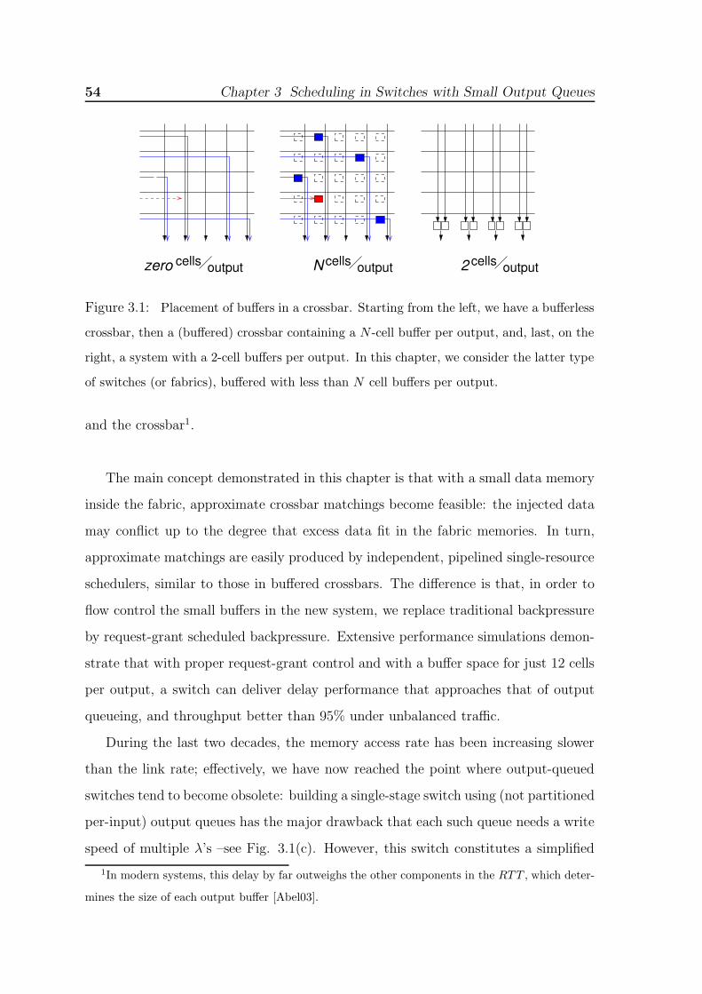
54 Chapter 3 Scheduling in Switches with Small Output Queues
cells output cells outputcells output N 2zero
Figure 3.1: Placement of buffers in a crossbar. Starting from the left, we have a bufferless
crossbar, then a (buffered) crossbar containing a N -cell buffer per output, and, last, on the
right, a system with a 2-cell buffers per output. In this chapter, we consider the latter type
of switches (or fabrics), buffered with less than N cell buffers per output.
and the crossbar1.
The main concept demonstrated in this chapter is that with a small data memory
inside the fabric, approximate crossbar matchings become feasible: the injected data
may conflict up to the degree that excess data fit in the fabric memories. In turn,
approximate matchings are easily produced by independent, pipelined single-resource
schedulers, similar to those in buffered crossbars. The difference is that, in order to
flow control the small buffers in the new system, we replace traditional backpressure
by request-grant scheduled backpressure. Extensive performance simulations demon-
strate that with proper request-grant control and with a buffer space for just 12 cells
per output, a switch can deliver delay performance that approaches that of output
queueing, and throughput better than 95% under unbalanced traffic.
During the last two decades, the memory access rate has been increasing slower
than the link rate; effectively, we have now reached the point where output-queued
switches tend to become obsolete: building a single-stage switch using (not partitioned
per-input) output queues has the major drawback that each such queue needs a write
speed of multiple λ’s –see Fig. 3.1(c). However, this switch constitutes a simplified
1In modern systems, this delay by far outweighs the other components in the RTT , which deter-
mines the size of each output buffer [Abel03].

3.2 Switch architecture 55
model preparatory for the multistage fabric studied in chapters 4 and 5; with this
in mind, besides their theoretical importance, the results that we present in this
chapter are of interest primarily for large, multistage fabrics, built out of several
smaller switches. Even if each switch is internally organized as a buffered crossbar,
the available buffer space on the path to each fabric output will be significantly smaller
than N , i.e. the number of input linecards. In chapters 4 and 5, we incorporate a
scheduling subsystem, similar to the one introduced here, in such large fabrics.
3.2 Switch architecture
Following the motivation of the previous section, this section presents the architecture
and the performance of the new switch model, with N small output queues. The new
architecture uses request-grant scheduled backpressure in order to control output
queue usage.
3.2.1 Queueing and control
For simplicity, we will consider fixed-size packets, called cells2. Storage for cells is
provided in large virtual output queues (VOQs) maintained in the ingress linecards.
A small contention resolution buffer, with capacity for B cells, is placed in front of
each output port of the switching fabric. All ports in and out of the fabric run at the
line rate (λ), as we do not use any internal speedup. The lack of speedup eliminates
the need for queues in the egress linecards.
To reduce the aggregate memory throughput, one can organize the output queues
inside a shared-memory. The scheduling unit that we describe below explicitly up-
per bounds the size of each individual output queue, thus avoiding memory space
monopolization by congested outputs.
The scheduling unit is depicted in Fig. 3.2. Before injecting a cell into the fabric,
a VOQ must first reserve a slot (secure a credit) in the buffer of the corresponding
2As outlined in section 2.1.1, we can support variable-size packets with no segmentation overhead,
by injecting variable-size segments upon grant receipt.

56 Chapter 3 Scheduling in Switches with Small Output Queues
SS
SS
N
1
Nλ
λ λ
λ
1λ
λ
VOQs
VOQs
req.
credit/gr.
cred
it/gran
t
request
grant grantcnts
requestcnts
creditschedulersschedulers
SDScheduling DelayProp. Time
1 grant/cell−timerate
inpu
ts
outp
uts
size Blinecards switch or fabricP rate R
reque
st
Figure 3.2: A switch with small output queues managed using request-grant scheduled
backpressure.
output port. For that purpose, linecards issue requests from VOQs to a control
unit. The control unit comprises N (per-output) credit schedulers, and N (per-input)
grant schedulers. Requests are routed to the credit scheduler that corresponds to the
intended output, and are registered in request counters, organized per (input-output
pair) flow. When its credit counter is zero, or when all its request counters are zero,
the credit scheduler stays idle; otherwise, it selects one among the non-zero request
counters, and issues a credit to the corresponding input. At this point, the credit
counter and the selected request counter are decremented by one. We denote by Rc
the peak rate at which credit schedulers can issue credits.
Unmatched inputs, waiting for credit, are allowed to send new requests to the
same or to other outputs. As credit schedulers work independently, multiple credits,
from different outputs, can be issued concurrently to the same input. All credits
issued to an input are first registered in per-flow grant counters. The grant scheduler
for an input selects one non-zero grant counter at a time, decrements it by one, and
sends a grant to the corresponding ingress linecard. We denote by Rg the peak rate
at which a grant scheduler can send grants, and we consider that Rg equals one grant
per cell time.

3.2 Switch architecture 57
Upon receiving a grant for output j, linecard i immediately forwards the HOL
cell of VOQ i→j to the switch. This cell is guaranteed to find an available slot in
the targeted output queue. Once the cell departs from that output queue, a credit is
returned to the corresponding credit scheduler. Besides cell forwarding, the received
grant allows for a new i→j request to be sent from ingress linecard i, if flow i→j has
enough cells in its VOQ. At start time, each flow is allowed to send up to u requests
before receiving any grant back; after u requests have been sent, new i→j requests
are refrained until the first i→j grant arrives. This request control equalizes, in the
mid to long term, a flow’s request rate with its grant rate. Note that u must be set in
accordance to the request round-trip time, which spans from the time a VOQ issues
a request, to the time it receives the respective grant (see section 2.1.1).
3.2.2 Common-order round-robin credit schedulers
The default credit scheduling discipline that we consider is pointer-based round-robin.
To determine which input to grant to, a scheduler scans among inputs 1 to N , circu-
larly, starting from the input indicated by a next-to-serve pointer. The first eligible
input found, e is served, and next-to-serve advances to (e+1) modulo N . If no input
is eligible, the next-to-serve pointer stays intact. In the baseline implementation,
all output schedulers use a common ordering of inputs, in their round-robin frames;
we will see later (section 3.6) that such a common order causes some performance
problem, and we will modify it accordingly.
The default grant scheduling discipline is defined as above, substituting term input
for term output, and vice versa, wherever appropriate.
3.2.3 RTT & output buffer size
The small output buffers used in our system resolve conflicts that occur when mul-
tiple inputs concurrently receive grants from the same output; in the worst case, k=
min(N ,B) inputs may conflict in that way. But how large output buffers do we need?
Roughly speaking, the larger the output buffer the better the performance; however,
the simulation results that we present in subsequent sections indicate that increasing

58 Chapter 3 Scheduling in Switches with Small Output Queues
this buffer space beyond 12 cells per output offers marginal only performance benefits.
In the present section, however, we are interested in a different question: what is
the minimum buffer size required to support persistent, non-contenting connections?
Let P be the (one way) propagation delay between the linecards and the fabric, and
SD be the delay of a request going through both credit and grant scheduling inside
the control unit. We define the round-trip time, RTT , to be the minimum delay
(i.e. assuming that no contention is present) between the issuing of a credit by a
credit scheduler, until the cell injected owing to that credit exits the switch, and
the corresponding credit returns to the same credit scheduler and is re-issued again
(credit cycle). Each output buffer must have a size greater than or equal to one such
RTT worth of cells. This RTT comprises the latency of grant scheduling, one P delay
until the grant reaches the ingress linecard, one additional P delay taken by the cell
to reach the fabric, and the latency of credit scheduling3; thus, RTT= 2 · P + SD.
To keep its corresponding link busy, each credit (output) or grant (input) scheduler
needs to serve a new request or grant, respectively, per cell time. Thus, the maximum
available “thinking time” for each such scheduler is one cell time, and SD ≤ 2 cell
times. In section 3.3, we will introduce a novel method that eliminates the component
2 · P from the above equation. Thus, by setting SD= 2, and neglecting P , we get
that RTT= 2 cell times, thus B ≥ 2 cells.
3.2.4 Scheduler operation & throughput
The scheduling subsystem is depicted in Fig. 3.3. This organization of credit
(output) and grant (input) schedulers resembles schedulers for bufferless crossbars,
like iSLIP, but when B≥ 2 cells, the present scheme is simpler, since there is no need
for schedulers to coordinate their decisions on an individual cell time basis, like they do
3The RTT must also include several other “minor” delays: (i) the time needed to fetch the cell
from its VOQ, (ii) the cell delay inside the fabric chip, and (ii) the time it takes for the released
credit to reach its credit scheduler (we assume that the credit schedulers reside in the same chip
with output queues).

3.2 Switch architecture 59
cnt
cnt
cnt
cnt
cnt cnt
cnt
cnt
cnt
cnt cntcnt
cnt cntcnt
S S SS
cntS
S
S
inp 1
inp 2
inp 3
inp 4outp 2
outp 3
outp 1
S r
eque
st c
ount
ers
outp 4
grant counters
Figure 3.3: The scheduling subsystem for a 4 × 4 VOQ switch with small, shared output
queues; the per-output (credit) schedulers and per-input (grant) schedulers form a 2-stage
pipeline, with the request and grant counters acting as pipeline registers.
in iSLIP; instead, they can operate independently, in a two-stage pipeline: in the first
pipeline stage, each credit scheduler independently produces a grant and increases
by one the corresponding grant (pipeline) counter; in parallel with the first stage
operations, each grant scheduler (second pipeline stage) independently selects one
among the grants accumulated up to now inside its grant counters –not yet considering
the concurrent outcomes by the credit schedulers. The matchings produced in this
way may conflict with each other, but that does not matter: if multiple ingress
linecards receive a grant for the same output at the same time, the output buffer
will absorb the resulting conflict. Actually, thanks to request and grant buffering, all
schedulers inside the control unit can work asynchronously. This type of scheduling
is as simple as buffered crossbar scheduling.
Deterministic 100% throughput when B = 1 cell, under uniform load
Assume that P= 0. When B= 1 cell, output credit schedulers reduce to link sched-
ulers, and the scheduling control unit reduces to a bufferless crossbar scheduler. As in
bufferless crossbars, a complete scheduling operation, comprising both output (credit)

60 Chapter 3 Scheduling in Switches with Small Output Queues
and input (grant) scheduling, has to complete within the boundaries of a single cell
time (SD ≤ 1 cell time).
Under uniform load, this system deterministically achieves 100% throughput. To
see why, observe that with B= 1, any particular credit scheduler may have only one
input granted at any given time –it can issue a new grant only after it is notified
that its previous grant has been accepted, when the corresponding cell departs from
the output buffer. If this output grant is not selected by the grant scheduler, it
will reside in its grant queue (counter), waiting to be served, which is equivalent
to what happens in iSLIP –and, symmetrically in DRRM [YLi01]: iSLIP, instead
of storing unaccepted grants, cancels them, but reproduces them in subsequent cell
times until they get accepted. Thanks to these persisting grants, output schedulers
desynchronize, and 100% throughput is achieved under uniform load –see Fig. 3.4(a).
A formal proof for this 100% throughput capability can easily be derived as in [YLi01]
–we skip the details, because they are identical to the proof in that work. Note that,
as in iSLIP, common-order round-robin output credit schedulers are a requisite for
desynchronization.
Statistical desychronization
For the more practical system, with two cell times pipeline scheduling latency (SD=2),
and B ≥ 2, a possible proof for the 100% throughput capability would not be trivial
at all. The problem lies in that we cannot easily identify the input that an output will
issue a credit to, after it receives a credit back from a grant scheduler, since it may
have already served several subsequent inputs, utilizing one of its additional credits.
Nevertheless, our simulation results indicate that 100% throughput is achieved when
SD= 2 and B= 2; moreover, as shown in section 3.4.4, in terms of delay, this more
practical system outperforms the previous one, for which we have proved the 100%
capability.
Whereas for B= 1 full desynchronization is needed in order to achieve 100%
throughput, for B≥N throughput is not wasted even if output schedulers get com-

3.2 Switch architecture 61
RR RR RR RR RR
RR
RR
RR
RR
RR RR
RR
RR RR
RR
RR
RR RR
RR
RR
RR
RR
RR
RR
RR
RR
1
RR
RR
RR
RR RRRR
RR
RR
RR RR
RR
RR RR
RR
RR
RRRR
RR
RRRR
credit grant creditgrant grant credit grant credit
credit grant creditgrant grant credit grant credit(output)(input)(output)(input)(output)(input)(output)(input)
3 3 3 333
2
11
1
111
1
1
11
2 2
1
22 2
1
(output) (input) (output) (input) (output) (input) (output)(input)
1
2
RR1 1
2 2
1 1 1
1
313
2
1
2
3
111
1
112
1 1
3
111
2
1
11111
1
2
3 3
111
1
2
33
2
1RR
3 31
1
1
(a) desynchronization with 1 credit available per output
cell time 1 cell time 2 cell time 3 cell time 4
(b) full throughput with 3 (=N) credits available per output
issued creditsgrant cnts
returnedcredits
Figure 3.4: (a) when B= 1 (similar to bufferless crossbars), schedulers deterministically
desynchronize and achieve 100% throughput; (b) when B= N (similar to buffered crossbars),
100% thoughput is achieved even when schedulers are fully synchronized.
pletely synchronized –see Fig. 3.4(b). For intermediate values of B, between 1 and N ,
we need credit schedulers to desynchronize to some extent. This desynchronization
need not be deterministic, but can be of statistical nature. Since there are N×B cred-
its available, and only N inputs, each input will normally have an adequate backup
supply of credits to use, even if it does not get a new grant in some specific cell
time. To this end, output pointers do not have to “lock” in some particular arrange-
ment, like they have to in bufferless crossbars; they simply need to avoid degenerate,
synchronized behavior.
A simple model will help us support this intuitive idea. Assume that every output
credit scheduler holds B credits, which it distributes uniformly, and at random, to
N inputs4. After all outputs have distributed their credits, the probability that an
input has no credit is p= (1− 1N
)(N ·B). In Fig. 3.5, we plot this average percentage of
4The allocation of each individual credit is modeled as an independent process, wherein each
input has probability 1
N of receiving the next credit.
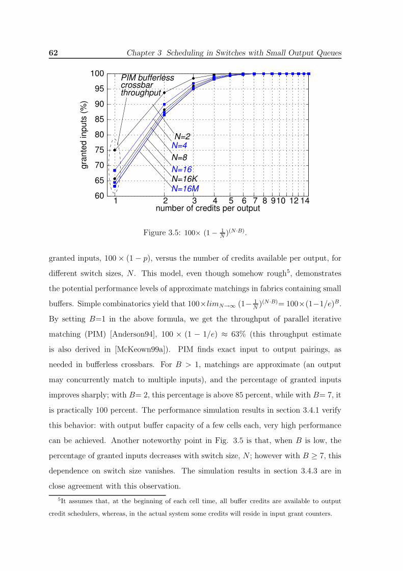
62 Chapter 3 Scheduling in Switches with Small Output Queues
N=8
N=16K
N=4
N=16
N=16M
N=2
PIM bufferlesscrossbarthroughput
14 12 10 9 8 7 6 5 4 3 2 1number of credits per output
60
65
70
75
80
85
90
95
100gr
ante
d in
puts
(%)
Figure 3.5: 100× (1− 1N )(N ·B).
granted inputs, 100× (1− p), versus the number of credits available per output, for
different switch sizes, N . This model, even though somehow rough5, demonstrates
the potential performance levels of approximate matchings in fabrics containing small
buffers. Simple combinatorics yield that 100×limN→∞(1− 1
N)(N ·B)= 100×(1−1/e)B.
By setting B=1 in the above formula, we get the throughput of parallel iterative
matching (PIM) [Anderson94], 100 × (1 − 1/e) ≈ 63% (this throughput estimate
is also derived in [McKeown99a]). PIM finds exact input to output pairings, as
needed in bufferless crossbars. For B > 1, matchings are approximate (an output
may concurrently match to multiple inputs), and the percentage of granted inputs
improves sharply; with B= 2, this percentage is above 85 percent, while with B= 7, it
is practically 100 percent. The performance simulation results in section 3.4.1 verify
this behavior: with output buffer capacity of a few cells each, very high performance
can be achieved. Another noteworthy point in Fig. 3.5 is that, when B is low, the
percentage of granted inputs decreases with switch size, N ; however with B ≥ 7, this
dependence on switch size vanishes. The simulation results in section 3.4.3 are in
close agreement with this observation.
5It assumes that, at the beginning of each cell time, all buffer credits are available to output
credit schedulers, whereas, in the actual system some credits will reside in input grant counters.

3.3 Credit prediction: making buffer size independent of propagation delay 63
3.3 Credit prediction: making buffer size indepen-
dent of propagation delay
The request-grant flow control scheme, as presented so far, reserves a separate buffer
slot for every cell or grant in transit between the linecards and the fabric. In effect,
the output buffer size computed in section 3.2.3 grows linearly with the propagation
delay, P . In this section, we introduce a novel scheme which eliminates P from
the effective round-trip time used in dimensioning the output queues. To do so, we
will first consider that departures from output queues are never blocked by external
backpressure; later on, we will relax this restriction.
Credits are generated when cells depart through the fabric-output ports. Since
there is no external backpressure to these ports, if we know that an output queue will
be non-empty at a given time in the future, we can predict that a cell will depart and
a credit will be generated (per cell time) at that time in the future. Such predicted
“future credits” can be used to trigger cell departures from the ingress linecards,
provided we can guarantee that the corresponding cells will not arrive at the buffer
before the above future time. In our case, consider a grant g selected at time t by a
grant scheduler; g will arrive at its linecard at t + P , will trigger the corresponding
cell departure, and that cell will arrive into its output buffer at t + 2P . At time t we
know g, hence we also know the output that it refers to; thus, we can safely conclude
that that output will be non-empty at time t + 2P , and consequently it will generate
a credit at t + 2P + 1. At t + 1 we can use this predicted credit to generate a grant,
given that the latency from grant generation to cell arrival at the output buffer can
never be less than 2P .
For the scheme to work correctly we must take care of one additional issue. Say
that at time t, k (> 1) grants for output o are selected by k grant schedulers in
parallel. In this case, under credit prediction, k credits must be returned to the
corresponding credit scheduler. However, observe that the credit count should not be
incremented by k at once at time t, since the credit scheduler for output o may then
drive multiple (>1) cell arrivals in time t + 2P + 1 (assuming Rc>1), whereas only

64 Chapter 3 Scheduling in Switches with Small Output Queues
one new cell position in the buffer will become available at that time. In order to
guarantee no buffer overflows, we throttle credit increments so that these occur at a
peak rate of one (credit) increment per cell time and per output. This can be realized
using an intermediate predict credit counter, in addition to the actual credit counter
used so far. The predict credit counter, which is initialized at zero (0), is incremented
every time a grant for that output is sent to an input line-card, and is decremented
by one in every new cell time when it is greater than zero; once decremented, the
corresponding (actual) credit counter is incremented by one. Observe that when Rc=
1, the need for the predict credit counter is obviated: each credit scheduler always
allocates only one new credit per cell time.
Using credit prediction, a credit can be reused just after the input grant scheduler
selects it. Thus, the RTT is reduced from its original value of 2 ·P +SD to just SD.
When the demand for an output is high, cells and grants for this output, of aggregate
volume 2P × λ, will be virtually “stored” on the lines between the linecards and the
fabric6.
3.3.1 Circumventing downstream backpressure
Now we will modify credit prediction to account for credit-based backpressure, ex-
erted upon fabric-output ports from nodes in the downstream direction. It makes no
difference whether these nodes be the egress linecards of the present switch or the
ingress linecards of the downstream neighbor: when backpressure is present, credit
prediction, as described so far, is not valid: the fact that a queue will be non-empty
at time t+2P no longer guarantees that the queue will generate a new credit at that
time, since departures from output queues can be blocked at any time. We can work
6A final economy on buffer space is possible –probably suitable for optical switches. We can
implement single-cell output queues, and permit two pending grants per-output, as needed in order
to compensate for the 2-cell time pipeline scheduling latency. When two cells concurrently arrive
at an output, one of them will be stored inside the output buffer, while the other one will bypass
the buffer on its way to the output. In the next cell time, the stored cell can depart for the output.
Assuming Rc=1, at most one new cell will arrive in this next cell time. The new cell can be stored
inside the output queue, while the previously stored cell departs.

3.4 Performance simulation results: part I 65
around this problem, if, instead of examining the downstream backpressure state at
the output ports of the fabric, i.e. for cells that have already reached their output
queue, we consult downstream backpressure before issuing new grants.
Each credit scheduler maintains two credit counters: the fabric credit counter that
holds the number of available cell positions in its corresponding output buffer, and
an additional downstream credit counter used for external backpressure purposes. Up
to now, it was safe to issue a credit as long as the fabric credit counter is non-zero;
to account for external backpressure as well, we require that the downstream credit
counter also be non-zero. After issuing a credit, both credit counters are decremented;
the fabric credit counter is incremented after grant scheduling, using credit prediction
rules, whereas the downstream credit counter is incremented when credits from the
downstream node reach the credit scheduler7.
3.4 Performance simulation results: part I
In this section we evaluate the performance of the switch with small output queues by
means of simulation experiments. The simulation environment and the traffic patterns
are described in Appendix B. In all experiments presented in this chapter, parameter
u is set equal to 10000. Credit prediction is used only in simulation experiments
where this is explicitly stated.
3.4.1 Effect of buffer size, B
In our first simulation experiment, we use uniformly-destined, Bernoulli cell ar-
rivals, and we examine the effect of the buffer space, B, on performance. For com-
parison, we also present the performance of iSLIP (iterations 1, 2 and 4), and of a
buffered crossbar switch with one cell buffer per crosspoint (bufxbar). All switches
have 32 ports. Fig. 3.6 presents average cell delay versus input load. A first point is
7Observe that this method increases the effective round-trip time pertaining to the downstream
(external) backpressure by the (internal) scheduler-linecard round-trip time.

66 Chapter 3 Scheduling in Switches with Small Output Queues
B1B12B8
B2 B4
1SLIP
2SLIP
bufxbar
0.01
0.1
1
10
100
1000av
erag
e de
lay
(cel
l−tim
es)
0.1 0.2 0.3 0.4 0.5 0.6 0.7 0.8 0.9 1normalized input load
Figure 3.6: Performance for varying buffer size, B; N= 32, P= 0, Rc= 1, and SD=1;
Uniformly-destined Bernoulli cell arrivals. Only the queueing delay is shown, excluding all
fixed scheduling and propagation delays.
that thanks to the desynchronization effect, our system, for any B value, saturates
when the (normalized) input load approaches unity. B1 behaves very close to 1SLIP
for the reasons described in section 3.2.4. With increasing B, it happens less fre-
quently that a backlogged input does not receive any grant, therefore delay improves;
B12 approaches the delay of bufxbar. Under smooth arrivals, we found no benefit in
further increasing B.
One may observe that, under medium input load, our system exhibits slightly
higher delay than bufxbar. This can be ascribed to the following behavior: at medium
load, occasional small bursts of cells for a switch output, from different inputs, enter
the fabric of our switch only at the rate the credit scheduler admits cells inside, i.e.
Rc= 1 cell (credit) per cell time; in the buffered crossbar, such small bursts may
enter the fabric immediately, regardless of output contention. In our system, these
“deferred” admissions marginally increase input contention and thereby cell delay.
The following section supports this argument.

3.4 Performance simulation results: part I 67
0.2 0.3 0.4 0.5 0.6 0.7 0.8 0.9 1normalized input load
R4
bufxbar
B=4
R1.5R2
0.01
0.1
1
10
100
1000
0.1
aver
age
dela
y (c
ell−
times
)
R1
Figure 3.7: Performance for varying credit scheduler rate, Rc; N= 32, P= 0, SD= 1, and
B= 4; Uniformly-destined Bernoulli cell arrivals. Only queueing delay is shown, excluding
all other fixed delays.
3.4.2 Effect of credit rate, Rc
In this experiment we change the rate Rc, at which credit schedulers issue credits8.
Figure 3.7 shows our results. We see that, for Rc> 1, cell delay at medium loads
approaches buffered crossbar delay, because of more cells skipping input contention.
Under high load, increasing Rc above 1 credit/cell-time does not improve delay. The
following observation explains this behavior.
Credits are usually pending: When the load approaches unity, credit sched-
ulers will usually have allocated all their credits to inputs. This happens due to
random grant conflicts, which unavoidably delay the return of some credits. There-
fore, as credit schedulers are greedy, issuing 1 credit per cell time, soon their whole
available credit moves into input grant counters. After this point is reached, on av-
erage one new credit becomes available per output in each new cell time, and that is
immediately issued to some of the requesting inputs. Therefore, even if Rc >1, the
effective credit rate equals one for most of the time.
8Grant schedulers operate at their default rate of one grant per cell time.

68 Chapter 3 Scheduling in Switches with Small Output Queues
B1
plots matchN64, for B12:
N128
N64N32
and N32N128,N256,
0.2 0.3 0.4 0.5 0.6 0.7 0.8 0.9 1normalized input load
0.1 0.01
0.1
1
10
100
aver
age
dela
y (c
ell−
times
) 1000
Figure 3.8: Performance for varying sw. size, N ; P= 0, Rc= 1, and SD= 1; Uniformly-
destined Bernoulli cell arrivals. Only queueing delay is shown, excluding all other fixed
delays.
3.4.3 Effect of switch size, N
In Fig. 3.8, we evaluate the effect of switch size, N . We find that, when B
is small, performance deteriorates with increasing N . (Iterative crossbar arbiters
exhibit similar behavior.) When B= 1, this dependance on switch size appears for
input loads above 0.5. At such loads, uncoordinated, random scheduling decisions
fail to drain VOQs9, and the need for desynchronization emerges. In the lack of
desynchronization, VOQs, and thus delays, grow. But desynchronization takes time
proportional to N [YLi01], which roughly explains this dependence on switch size.
As discussed in section 3.2.4, with increasing B, the dependence on switch size
vanishes thanks to statistical desynchronization. This is validated in Fig. 3.8: with
B= 12 cells, delay is identical for all switch sizes, N = {32, 64, 128, 256}.9As discussed in section 3.2.4, PIM algorithm, which uses random schedulers, saturates at a load
close to 0.63.

3.4 Performance simulation results: part I 69
3 matching plots for B12and all of SD=0,1,2
B2−SD=2, 1, 0
B1−SD=1, 0
0.01 0.1 0.2 0.3 0.4 0.5 0.6 0.7 0.8 0.9 1normalized input load
0.1
1
10
100
1000
aver
age
dela
y (c
ell−
times
)
Figure 3.9: Performance for varying scheduling delay SD, and varying buffer size B; N=
32, P=0, Rc= 1; Uniformly-destined Bernoulli cell arrivals. Only queueing delay is shown,
excluding all other fixed delays.
3.4.4 Effect of scheduling and propagation delays
All plots presented so far assumed scheduling delay, SD equal to one cell time.
Remember that SD is the latency incurred while a request goes through credit and
grant scheduling. A value of SD equal to one cell time is the maximum allowable
when B= 1, i.e. when the scheduler finds exact input/output matchings. But when
B ≥ 2, SD can be as large as two cells times.
In Fig. 3.9, we present three groups of plots: one for B= 1 (SD equal to 0 and
1), one for B= 2 (SD equal to 0, 1, and 2) , and one for B= 12 (SD equal to
0, 1, and 2). As the figure shows, when B equals one or two, a smaller SD value
delivers discernibly lower queueing delay. We conjecture that, with a small SD value,
schedulers’ coordination speeds up (credits return sooner to credit schedulers), thus
configurations with a small number of available credits (B) benefit. But with B= 12,
the dependance of queueing delay on coordination latency vanishes.
Next, in Fig. 3.10, we examine how performance is affected when propagation

70 Chapter 3 Scheduling in Switches with Small Output Queues
3 matching plots for B2, and all of P=0, 1, 100
B12, P100
with credit prediction, SD2
no credit predictionSD2, P1
B2 B4
0.01
0.1
1
10
100
1000av
erag
e de
lay
(cel
l−tim
es)
0.1 0.2 0.3 0.4 0.5 0.6 0.7 0.8 0.9 1normalized input load
Figure 3.10: Performance for varying scheduling delay SD, and varying P , with, and
without, credit prediction; N= 32, Rc= 1; Uniformly-destined Bernoulli cell arrivals. Only
queueing delay is shown, excluding all other fixed delays.
delay increases. A first observation is that, when credit prediction is employed, the
queueing delay does not depend on the propagation delay, P : with constant B, the
switch performed equally well for all P values examined (0, 1, and 100 cell times).
On the other hand, if we do not apply credit prediction, output buffers will need a
size proportional to 2P . This is manifested via the no credit prediction curves. In
these configurations, RTT (= 2P + SD) equals four cell times, as SD= 2 and P=
1; hence, for B= 2, the scheduler can achieve only half of the maximum throughput,
and performs satisfactory only for B= 4, or greater.
Figure 3.10 also shows that, with P= 100, SD= 2, and B= 12, the present sys-
tem performs very close to buffered crossbars (compare with Fig. 3.6). To appreciate
the buffer savings achieved by the present system, consider that a 32× 32 traditional
buffered crossbar, with 100 cell times propagation delay, requires 204 K cells of buffer-
ing, whereas the present system uses only 384 cells (not K cells) of total buffer space.
For a 64× 64 switch, the respective numbers would be 816 K cells of buffering for the
buffer crossbar, and 768 cells (not K cells) of buffering for the present system.

3.4 Performance simulation results: part I 71
0 0.2 0.4 0.6 0.8 1unbalance factor, w
0.6
.65
0.7
.75
0.8
.85
0.9
.95
1.0
norm
aliz
ed s
witc
h th
roug
hput
B1
B2 4SLIPbufxbar
B4B12
B64B32
1SLIP
Figure 3.11: Throughput performance under unbalanced traffic for varying buffer size, B;
N= 32, P= 0, Rc= 1, and SD=1; full input load.
3.4.5 Unbalanced traffic
In this section, we measure switch throughput under unbalanced, Bernoulli cell ar-
rivals –see appendix B. Traffic is uniformly-destined when w= 0, and completely
unbalanced (N non-conflicting, input i→ output i, connections) when w= 1. Our re-
sults, presented in Fig. 3.11, show that the throughput of B1 drops as low as 0.63 for
intermediate w values, similarly to iSLIP. With increasing B, throughput improves
fast; for B4, throughput is higher than 0.9, for B12 higher than 0.97, and for B32
higher than 0.99. The buffered crossbar (bufxbar) uses 1-cell buffer per crosspoint,
i.e. an equal amount of on-chip memory with B32, however its throughput is sig-
nificantly lower than B32. But even B4, which contains one eighth of the buffered
crossbar memory, achieves better performance than bufxbar. This is due to better
buffer sharing.
Under this traffic model, we can better understand the intuition that throughput
improves as the available buffer space per flow increases. Consider a heavily loaded
connection, f , from input i to output i. For intermediate w values, other flows origi-
nating from the same input with f toggle between active and inactive states. When
many of them are active, the input contention that f faces increases; symmetrically,

72 Chapter 3 Scheduling in Switches with Small Output Queues
bufxbar
OQ
1SLIP B4
B16B8
B2B32B64
1
10
100
1000
10000av
erag
e de
lay
(cel
l−tim
es)
0.1 0.2 0.3 0.4 0.5 0.6 0.7 0.8 0.9 1normalized input load
Figure 3.12: Performance under bursty traffic, for different buffer sizes, B, when no grant
throttling is used; N= 32, P= 0, Rc= 1, and SD= 1 cell time; average burst size 12 cells.
Only queueing delay shown, excluding all other fixed delays.
when multiple flows targeted to the same output as f are active, output contention
increases. The periods of increased input contention do not necessarily overlap with
the periods of increased output contention. Thus, there can be situations where many
input-“brothers” of f are active, whereas most of its output-brothers are inactive; in
this case, if there are not many cells of f stored inside the fabric in front of output
i, this output line will be underutilized. This observation explains things: a large
output buffer (B) absorbs f ’s traffic when output contention is high, and occupies
with that traffic the output line when input contention is high. In Fig. 3.11, the
bufxbar contains large, 32-cell, buffers per output, however, each flow can only access
its private, single-cell, crosspoint buffer; this justifies the relatively low throughput of
bufxbar.
3.4.6 Bursty traffic
The results presented so far were for smooth, Bernoulli cell arrivals. However,
several studies have shown that traffic in the Internet is correlated (bursty). Figure
3.12 depicts the delay performance under uniformly-destined bursty traffic with aver-

3.5 Throttling grants to a bottleneck input 73
age burst size equal to 12 cells. As can be seen, with B= 12, the delay of our system
is quite higher than that of the buffered crossbar; even worse, B must be significantly
increased in order to improve this delay. For any buffer size shown in the figure,
we can find a load point, l, after which, the delay of our switch grows sharply: for
B= 16, 32, and 64, l ≈ 0.9, 0.94, and 0.96, respectively. Previous studies suggest
that, before reaching saturation, cell delay is roughly proportional to average burst
size [Li92] [McKeown99a]. However, the delay of the present switch increases even
further. What kind of phenomena are hidden behind this behavior? The following
section dwells into switch dynamics in order to answer this question.
3.5 Throttling grants to a bottleneck input
In this section, we discuss the behavior of request-grant scheduling in switches with
small output buffers under bursty traffic. We attribute the large delays under this traf-
fic model to credit accumulations, which occur in transient, unbalanced VOQ states,
and we propose threshold grant throttling as a means to control credit accumulations.
3.5.1 Unbalanced transients with congested inputs
In any switch, there are situations where some flows are “bottlenecked” at their inputs,
rather than at their outputs: Packets may first accumulate at inputs due to output
contention; then output contention may go away, and multiple packets would be able
to depart simultaneously toward multiple outputs if they were not constrained by the
limited bandwidth of the input buffer and of the linecard. Unbalanced transients with
bottlenecked inputs appear continously under statistically multiplexed flows (even
when the long-term load is uniform and feasible), but get more severe under bursty
and heavy traffic. When output contention subsides for a while, a congested input
may receive multiple credits from different outputs at about the same time. Limited
by its link capacity, that input cannot make use of more than one credit per cell time,
thus underutilizing buffer credits. Even worse, as we describe next, a congested input
tends to accumulate an abnormaly high number of credits.
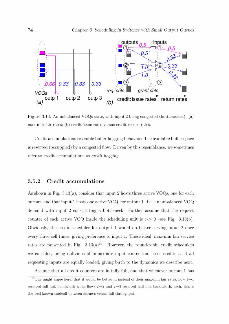
74 Chapter 3 Scheduling in Switches with Small Output Queues
outputs inputs
return rates
1 1
3
2
3
2
outp 3outp 2outp 1VOQs grant cnts
0.330.330.330.66
0.50.5
0.33
0.330.331.0
1.0
0.5
(a) issue ratescredit:
req. cnts
(b)
Figure 3.13: An unbalanced VOQs state, with input 2 being congested (bottlenecked): (a)
max-min fair rates; (b) credit issue rates versus credit return rates.
Credit accumulations resemble buffer hogging behavior: The available buffer space
is reserved (occuppied) by a congested flow. Driven by this resemblance, we sometimes
refer to credit accumulations as credit hogging.
3.5.2 Credit accumulations
As shown in Fig. 3.13(a), consider that input 2 hosts three active VOQs, one for each
output, and that input 1 hosts one active VOQ, for output 1 –i.e. an unbalanced VOQ
demand with input 2 constituting a bottleneck. Further assume that the request
counter of each active VOQ inside the scheduling unit is >> 0 –see Fig. 3.13(b).
Obviously, the credit scheduler for output 1 would do better serving input 2 once
every three cell times, giving preference to input 1. These ideal, max-min fair service
rates are presented in Fig. 3.13(a)10. However, the round-robin credit schedulers
we consider, being oblivious of immediate input contention, steer credits as if all
requesting inputs are equally loaded, giving birth to the dynamics we describe next.
Assume that all credit counters are initally full, and that whenever output 1 has
10One might argue here, that it would be better if, instead of their max-min fair rates, flow 1→1
received full link bandwidth while flows 2→2 and 2→3 received half link bandwidth, each; this is
the well known tradeoff between fairness versus full throughput.

3.5 Throttling grants to a bottleneck input 75
0.5
0.50.5
inputs
0.33
0.33
0.33
1
2
3
1
3
2
0.33
0.33
0.66
0.330.33 1.01.00.33
0.660.330.5
0.50.5
occasionally off
(a)
outputs
(b)
(iii)(ii)
(i)
inputsoutputs
1.01.0
Figure 3.14: Due to the rate mismatch in Fig. 3.13(b), (a) credits accumulate in front of
congested input 2; (b) service rates when using threshold grant throttling.
credits available, it throws a coin to decide which input to serve. In this case, output
1 will issue credits to input 2 at 1/2 rate. However, input 2 also receives credits from
outputs 2 and 3. Therefore, whereas credits issued to input 1 are recycled after one
cell time, credits issued to input 2 are recycled after three cell times, on average.
Obviously, all output 1 credits will soon pile up in front of grant scheduler for input 2
–see Fig. 3.14(a). The service rate of input 1, x, will be x= (1/2)× y, where y is the
rate at which output 1 holds some credit. As output 1 holds no backup of credits,
y= 1/3 + x, where 1/3 and x express the rates that credits return to output 1 from
input 2 and input 1, respectively. Solving the above equations yields the suboptimal
rates x= 1/3 and y= 2/311; thus, the utilization of output 1 is 2/3 where it could be
full.
Fortunately, owing to the equalization of VOQ request and grant rates, this inef-
ficient credit allocation cannot last for long, since the rate at which each flow in the
bottleneck input issues new requests will be upper bounded by 1/3, and thus, request
queue 2→1 will eventually empty. Once this happens, output 1 will give preference
to input 1. However, the drain time of a request queue can be quite long, considering
that u, its peak size, must be set in proportion to the propagation delay between the
11We have verified these rates by simulation.
76 Chapter 3 Scheduling in Switches with Small Output Queues
linecards and the scheduler, P . While the transient is active, VOQs and delay grow.
What reduces performance in credit hogging situations is not that some input
holds a lot of credits, neither that outputs, which have the authority to issue credits,
have no credits available. The problem lies in the combination of these two factors.
As we have pointed out in section 3.4.2, when the load is high, credits are usually
pending inside grant counters even under smooth traffic. However, in the smooth
case credits are pending in the grant counters of multiple inputs, thus they tend to
recycle fast.
3.5.3 Grant throttling using thresholds
One straighforward solution to diminish credit accumulations is to limit the total num-
ber of pending requests from any given input, effectively decreasing input contention
among the reserved credits. However, an input could then consume its allowable re-
quests sending them to congested outputs, thus not being able afterwards to request
other, possibly lightly loaded destinations.
To control credit accumulations when inputs are allowed to have many outstanding
requests, the key idea is for credit schedulers to stop serving inputs that do not re-
turn credits fast enough. This method constitutes an equivalent of the “output queue
length threshold” method used in shared memory systems [Katevenis98] [Hahne98]
[Minkenberg00] ; in these systems, the target is to preclude cells destined to a con-
gested output from monopolizing the shared memory; in our case, the target is to
prevent a congested input from hogging buffer credits.
Let GQ(i) denote the cumulative grant queue size for input i. (This is the sum of
the current values of all grant counters corresponding to that input.) Our mechanism
changes the eligibility of input i for credit schedulers, taking GQ(i) into account: a
request from input i is eligible at its output (credit) scheduler, iff (a) output buffer
credits are available (this was always a requirement), plus additionally (b) GQ(i) is
less than a threshold, TH. Implementing threshold grant throttling requires that
each grant scheduler i circulates a common On/Off signal to all credit schedulers,
that stays Off whenever GQ(i) ≥ TH.

3.5 Throttling grants to a bottleneck input 77
no grant throttling
TH15with grant throttling
1−SL
IP
OQ
and OQ plots matchTH7, TH5, TH3
0.1 0.2 0.3 0.4 0.5 0.6 0.7 0.8 0.9normalized input load
1 1
10
100
1000
10000
aver
age
dela
y (c
ell−
times
)
Figure 3.15: Performance under bursty traffic, for different grant throttling thresholds,
TH; N= 32, B= 12; average burst size 12 cells; Only the queueing delay is shown, excluding
all other fixed delays.
Certainly, threshold TH must be set below B, since the average GQ is ≤ B.
To make the method more reactive, a low threshold is appropriate. On the other
hand, too low a threshold may put at risk schedulers’ flexibility: if all inputs block,
output schedulers will not be able to produce new grants, and buffer space may be
underutilized.
Returning to the example depicted in Fig. 3.13, our simulations showed that,
with threshold grant throttling, the switch delivers the ideal rates. Figure 3.14(b)
depicts how this happens. Whenever the grant queue backlog in front of input 2
reaches threshold, TH, input 2 turns Off. Effectively, the credit scheduler for output
1 adapts the rate at which it issues credits to input 2 to the rate that input 2 returns
these credits back, i.e. 0.33. At times when input 2 is Off, output 1 issues credits to
input 1, increasing the rate of flow 1→1 to 0.66.

78 Chapter 3 Scheduling in Switches with Small Output Queues
3.5.4 Effect of grant throttling under bursty traffic
Figure 3.15 presents delay performance under uniformly-destined traffic, with average
burst size equal to 12 cells. The output buffer size, B equals 12 cells. We can see
that, when no grant throttling is employed, or when TH>B (TH-15), the delay of
our switch is quite above that of pure output queueing (OQ). But, by using a threhold
below B (TH= 3, 5, and 7) delay essentially matches that of OQ. Simulation results in
section 3.8.2 confirm this good performance for average burst sizes up to one hundred
cells long.
3.6 Rare but severe synchronizations
Using threshold grant thottling, the (cumulative) queue size in front of any grant
scheduler will always be ≤ TH+N -1. An input may end up with these credits, if all
(N) output schedulers serve it in synchrony when it is just below the threshold, TH.
We do not want an input to end up with that many credits, because it would then
hold roughly 1/B of the total credits in the system, which need to be distributed to
as many as N inputs, where B<N . But why should output credit schedulers get that
coordinated?
Threshold grant throttling, not only does not prevent synchronizations, but it
may indirectly induce them. This section (a) describes this phenomenon, (b) shows
that it is due to all credit schedulers using the same round-robin order, while it is
also assisted by threshold grant throttling, and (c) proposes simple and efficient ways
to remedy this problem.
We will use the following terminology. We say that two or more credit schedulers
clash when they issue credits to (serve) the same input at the same time; we say that
two or more credit schedulers are synchronized, when their “next-to-serve” pointers
point the same input.

3.6 Rare but severe synchronizations 79
normal, uniform credit allocationthroughput close to 99%
inpu
t 15 input 21
input 21
inpu
t 15
inpu
t 15 input 21
input 21
inpu
t 16input 21
degenerate credit allocation byoutputs: throughput close to 85%
(similar, not shown peaks on inputs 16−20)
synchronizedco
mbi
ned
gran
t que
ue s
ize
cell−time
66
50 45 40 35 30 25 20 15 10 5 0
5020 5040 5060 5080 25020 25040 25060 25080 25100 5000 . . .
Figure 3.16: Evolution of combined grant queue size (GQ) in front of individual inputs,
while simulating a 32×32 switch, with B= 12 cells and TH= 7, under uniformly-destined,
Bernoulli traffic at 100% input load.
3.6.1 Experimental observations
Using common-order round-robin credit schedulers (section 3.2.2), we have observed
severe synchronizations under uniform traffic, when all VOQs become persistent12.
Under these traffic conditions, the synchronized schedulers clash, thus hurting switch
throughput.
Figure 3.16 depicts the time evolution of cumulative grant queue size, GQ, in front
of individual inputs. Data were recorded while simulating a 32× 32 switch (B= 12)
with grant throttling threshold TH= 7. The switch was fed with uniformly-destined,
Bernoulli cell traffic, at 100% load. For readability, we show only inputs 15 and 21.
Before cell time 20000 (left plot), when synchronization has not yet prevailed, GQ(15)
and GQ(21) evolve more or less normally, and switch throughput exceeds 98%. But
after cell time 20000 (right plot), synchronization is so severe that each input in turn
is concurrently granted by as many as 20 outputs. The time-axis distance between
the peaks in the graphs of inputs 15 and 21 is five cell times. In this interval, inputs
16-20 “collect” credits, one after the other, identically to inputs 15 and 21. The
figure on the right also shows that periodically some input stays with no grant (GQ=
0). In other words, statistical desynchronization is not full, explaining why switch
throughput drops down to 85%.
12These are the very same conditions that produce beneficial desynchronization in iSLIP

80 Chapter 3 Scheduling in Switches with Small Output Queues
outputs inputsoutputs inputs
cell time 2 cell time 3
inputs
Off
Off
outputs
cell time 1
1
2
3
4 4
3
2
1 1
2
3
4 4
3
2
11
2
3
4 4
3
2
11
2
3
4 4
3
2
1
serve
next−to−serve
Figure 3.17: How common-order round-robin credit schedulers, assisted by threshold
grant throttling, synchronize. Assume all inputs have request pending for all outputs, and
that TH= 2. Outputs are completely desynchronized in the beginning of cell time 1, and
one would expect them to remain desynchronized thereafter. The figure shows what will
happen if inputs 2 and 3 are Off in cell time 1, and turn On again in the beginning of cell
time 2.
3.6.2 Synchronization evolution
The cooperation of several independent behaviors is responsible for bringing the next-
to-serve pointers into degenerate situations. When the threshold TH is modest (<B)
and the load is high, it is reasonable to expect that some inputs will occasionally be
Off due to random grant conflicts. Assuming that the N next-to-serve pointers of the
credit schedulers are (still) in random, uniform positions, it is very likely that the very
first On input, say input i, whose order is next to a small sequence of consecutive Off
inputs, will receive more grants than usual. The reason is that all outputs pointing
somewhere in this sequence of idling inputs will stop “scanning” on input i. After
being granted by these many outputs, input i is likely to turn Off. In this way, in the
next cell time, input i will participate in a new sequence of idling inputs, therefore
reproducing the same phenomenon. But even worse, the output schedulers that served
input i in cell time t will be synchronized at input i + 1, in cell time t + 1. Through
this procedure, depicted in Fig. 3.17, more and more output schedulers synchronize.
It is interesting to note here that with bursty traffic the synchronizations are not

3.7 Round-robin disciplines that prevent synchronizations 81
as severe as with smooth Bernoulli traffic. Under bursty traffic, some VOQs (and
the respective request queues) may occasionally empty, effectively desynchronizing
output schedulers.
3.7 Round-robin disciplines that prevent synchro-
nizations
Since we want to preserve grant throttling in order to deal with unbalanced transients,
we next look for alternative credit scheduling disciplines that avoid synchronizations.
We found that neither fair queueing (FQ), nor random, credit schedulers suffer from
synchronizations of this kind. However, these schemes increase complexity, and we
do not study them further.
Synchronization prevails because, after a random grant conflict on input i in cell
time t, the clashing outputs synchronize again on input i + 1 in cell time t + 1.
In other words, the source of synchronizations is the common ordering in which all
credit schedulers visit and serve the input ports. But round-robin operation does not
presume a common or fixed order of service!
3.7.1 Random-shuffle round-robin
Our first method, depicted in Fig. 3.18, tackles “common ordering”. Each output
credit scheduler is preprogrammed with an ordering of inputs produced by some
random shuffle of the N inputs to the N positions in the round-robin “frame”. In
this way, even if pointers happen to clash in one cell time on some input, say on input
a, they will not necessarily synchronize in the next cell time, because each output sees
a different physical input as next to input a. We name this method random-shuffle.

82 Chapter 3 Scheduling in Switches with Small Output Queues
inputs inputsinputs
4
3
2
1
4
3
2
1
4
3
2
1
(a) (b) (c)
Figure 3.18: Possible round-robin scan orders for random-shuffle output credit schedulers.
In a 3×3 switch, orders (a), (b), and (c) could correspond to outputs 1, 2, and 3, respectively.
3.7.2 Inert round-robin
Another simple method maintains common ordering of inputs, but modifies the up-
date policy of next-to-serve pointers. Assume that this pointer had the value p and
that, searching from p onwards ended up serving input i. Then, instead of updat-
ing p to (i+1) mod N , we update p to (p+1) mod N . We name this scheme inert
round-robin.
Essentially, inert round-robin is a heuristic method. On the negative side, if the
distance between p and i is large, the same input i is likely to be serviced repeatedly
while p gets incremented by 1 every cell time, until it reaches i; however notice that
all inputs between p and i are ineligible, hence these either have not issued requests
or have already received many credits, thus it may be OK for i to be serviced multiple
times. On the positive side, schedulers will only synchronize in cell time t + 1 if they
were already synchronized in cell time t.
3.7.3 Desynchronized clocks
A nice modification to the previous scheme that deterministically desynchronizes out-
puts is the following. As with inert round-robin pointers, at start time each output

3.8 Performance simulation results: part II 83
points to a distinct input. From that point on, in each cell time, either all output
pointers advance by one, or all stay still. It is trivial to see that if the N “next-to-
serve” pointers go like this, hand-by-hand, they will never synchronize. It should be
made clear though that clashes can still occur when some connections are inactive.
The particular distributed policy that we propose advances all pointers in every
cell time, irrespective of whether each particular scheduler served a flow or not. We
call this discipline desynchronized clocks. A similar method has been proposed for
input scheduling in buffered crossbar switches [Han03] [Mhamdi04].
Our simulation results in section 3.8.1 show that the aforementioned methods pre-
vent synchronizations, and achieve nearly 100% throughput under uniformly-destined
load. Among them, only the random-shuffle method preserves the underlying round-
robin discipline. The other two methods, inert and desynchronized clocks, may be
unfair under particular circumstances. Consider for instance that an output is over-
subscribed by two persistent flows, one from input 0 and one from input 1. It is easy
to verify that inert and desynchronized clocks will allocate a bandwidth of 1/N to
input 1, and a bandwidth of (N − 1)/N to input 0.
3.8 Performance simulation results: part II
In this section, we evaluate by means of simulations the performance of the system
with threshold grant throttling, and credit scheduling disciplines that avoid severe
synchronizations.
3.8.1 Switch throughput under threshold grant throttling
In the first set of experiments, we measure switch throughput under unbalanced,
Bernoulli cell traffic, at 100% input load. As in section 3.4.5, traffic imbalance is
controlled by w: when w= 0 traffic is uniformly-destined, whereas when w= 1 traffic
consists of persistent, input-output, non-conflicting connections.

84 Chapter 3 Scheduling in Switches with Small Output Queues
TH<B
TH7
TH3TH5 TH3
TH5TH7
B32−TH7
buffer size B=12 cellsexcept B32−TH7
TH>=B:THInfTH15,TH12
0 0.2 0.4 0.6 0.8 1unbalance factor, w
1
.98
.96
.94
.92
.9
.88
.86
norm
aliz
ed s
witc
h th
roug
hput
Figure 3.19: Throughput performance under unbalanced traffic for varying buffer size, B,
and varying threshold values, TH, using common-order round-robin credit scheduling; N=
32; Bernoulli arrivals.
Common-order round-robin schedulers
Figure 3.19 depicts the switch throughput, using common-order round-robin sched-
ulers, for varying grant throttling threshold, TH; all plots are for B= 12 cells, except
for one, B32-TH7.
When the load is uniform (w= 0), the normalized throughput of configurations
with TH<B drops quite below 1, due to the synchronizations discussed in section
3.6. Only B32-TH7 keeps performing well, because it contains sufficient buffer space
per output –thirty-two cells, i.e. as many as N– to cope with synchronized schedulers
–see Fig. 3.4. Once w goes above 0, throughput improves considerably, because flows
alternate between active and inactive, and the synchronization behavior vanishes.
With TH≥B, throughput is high even when w= 0, as grant throttling only rarely
gets activated, and no massive scheduler synchronization appears.
At low w values, between 0 and 0.3, lower thresholds yield higher throughput,
because credit accumulation are more effectively controlled when grant throttling is
low. However, when the imbalance grows, this trend is reversed: higher thresholds

3.8 Performance simulation results: part II 85
shuffle:TH3,TH5, TH7
bufxbarbufxbar, CP4 CP12
clocks−TH5256−port
clocks:TH7,TH5, TH3
0.2 0.4 0.6 0.8 1unbalance factor, w
1
0
.99
.98
.97
.96
.95
.94
.93
norm
aliz
ed s
witc
h th
roug
hput
Figure 3.20: Throughput performance under unbalanced traffic for varying threshold, TH,
under different credit scheduling disciplines; B= 12 cells; all switches have 32 ports, except
one, 256-port clocks-TH5; Bernoulli arrivals.
yield higher throughput. At high imbalance, flows can be categorized in two distinct
groups: one flow per input (or per output) is heavy, while the remaining (light) flows
are almost always inactive, as they get served by the time they become active. Under
such load, a low TH value may prevent a heavy flow from receiving the excess service
available when its output neighbors are inactive, by frequently turning its input Off.
Random-shuffle & desynchronized clocks schedulers
Figure 3.20 depicts switch throughput, using random-shuffle (shuffle) and desyn-
chronization clocks (clocks) credit schedulers, for varying TH values. All plots are for
B= 12 cells. The main point in this figure is that these scheduling disciplines avoid
synchronizations for any TH value; in this way, uniform traffic throughput is well
above 99%. Both shuffle and clocks maintain a throughput above 0.96, even when
the traffic is unbalanced, with clocks performing slightly better. Simulation results,
not presented here, demonstrate that inert round-robin performs very close to clocks.
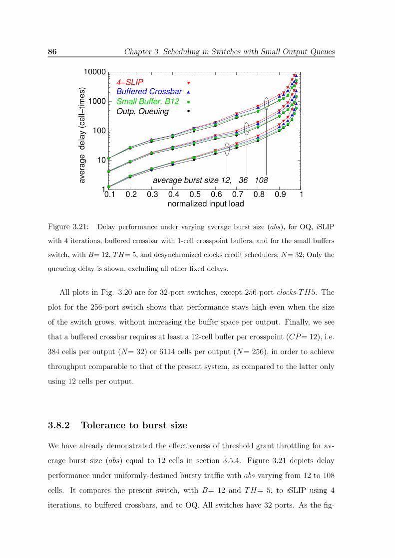
86 Chapter 3 Scheduling in Switches with Small Output Queues
Small Buffer, B12
4−SLIPBuffered Crossbar
Outp. Queuing
average burst size 12, 36 108 1
10
100
1000
10000
0.2 0.3 0.4 0.5 0.6 0.7 0.8 0.9 1 0.1normalized input load
aver
age
del
ay (c
ell−
times
)
Figure 3.21: Delay performance under varying average burst size (abs), for OQ, iSLIP
with 4 iterations, buffered crossbar with 1-cell crosspoint buffers, and for the small buffers
switch, with B= 12, TH= 5, and desynchronized clocks credit schedulers; N= 32; Only the
queueing delay is shown, excluding all other fixed delays.
All plots in Fig. 3.20 are for 32-port switches, except 256-port clocks-TH5. The
plot for the 256-port switch shows that performance stays high even when the size
of the switch grows, without increasing the buffer space per output. Finally, we see
that a buffered crossbar requires at least a 12-cell buffer per crosspoint (CP= 12), i.e.
384 cells per output (N= 32) or 6114 cells per output (N= 256), in order to achieve
throughput comparable to that of the present system, as compared to the latter only
using 12 cells per output.
3.8.2 Tolerance to burst size
We have already demonstrated the effectiveness of threshold grant throttling for av-
erage burst size (abs) equal to 12 cells in section 3.5.4. Figure 3.21 depicts delay
performance under uniformly-destined bursty traffic with abs varying from 12 to 108
cells. It compares the present switch, with B= 12 and TH= 5, to iSLIP using 4
iterations, to buffered crossbars, and to OQ. All switches have 32 ports. As the fig-

3.8 Performance simulation results: part II 87
average burst size 12 36
plots matchN32 andfor B=12 cells: N256
0.2 0.3 0.4 0.5 0.6 0.7 0.8 0.9 1normalized input load
1
10
100
1000
10000
0.1
aver
age
dela
y (c
ell t
imes
)
Figure 3.22: Delay performance under varying average burst size (abs), for the small
buffers switch, with B= 12, TH= 5, and random-shuffle credit schedulers; N= 32 and N=
256; Only the queueing delay is shown, excluding all other fixed delays.
ure shows, the present system, B12, achieves performance almost identical to OQ,
and better than 4-SLIP and buffered crossbar. These results are for 32-port switches
with clocks credit schedulers. Figure 3.22 shows that the shuffle credit schedulers
achieve similar delay; it also shows that a similar performance is achieved for 256-
port switches, without increasing buffer space per output.
3.8.3 Diagonal traffic
Last, we use another type of unbalanced traffic, named diagonal. Each input i injects
two active flows, flow i→i, and i→(i + 1) mod N . The former flow consumes two
thirds (2/3) of the incoming load, and the latter flow consumes the remaining one
third (1/3).
Figure 3.23 depicts the performance of our switch with TH= 5, and desynchro-
nized clocks credit schedulers, comparing it with that of 4-iteration iSLIP, of buffered
crossbar, and of output queueing (OQ). All switches have 32 ports. As the figure
shows, B12 saturates close to full input load, using either shuffle or clocks credit
schedulers, while the buffered crossbar saturates at 0.92 load, and 4-SLIP saturates

88 Chapter 3 Scheduling in Switches with Small Output Queues
OQ
4−SLIP
bufx
bar
B12: ,shuffle clocks
aver
age
dela
y (c
ell−
times
)
0.1 0.2 0.3 0.4 0.5 0.6 0.7 0.8 0.9 1normalized input load
0.1
10
100
0.01
1
Figure 3.23: Performance under diagonal traffic for OQ, iSLIP with 4 iterations, buffered
crossbar with 1-cell crosspoint buffers, and for the small buffers switch, with B= 12, TH=
5; N= 32; Bernoulli arrivals; Only the queueing delay is shown, excluding all other fixed
delays.
at 0.82 load.

Chapter 4
Scheduling in Non-Blocking
Three-Stage Fabrics
4.1 Introduction
It has been a longstanding objective to come up with an economic interconnection
architecture, scaling to large port-counts, and achieving sophisticated quality-of-
service (QoS) guarantees under unfavorable traffic patterns. Beyond 32 or 64 ports,
single-stage crossbar switches are quite expensive, and multistage interconnection net-
works (switching fabrics) become preferable; they are made of smaller-radix switching
elements (switches), where each such element is usually a crossbar. Theoretically, any
non-blocking multistage fabric has the capacity to perform equally well with single-
stage crossbars; however, in practice, handling the traffic that passes through such
networks is a complex distributed scheduling problem: output contention management
and in-order packet delivery are aspects of that endeavor.
This chapter lays out the fundamental scheduling methods that will allow us
to make a step towards practical three-stage, non-blocking, Clos/Benes networks in
chapter 5. The new scheduling architecture is based on request-grant backpressure,
and relies on multiple, independent, single-resource schedulers, operating in parallel
and in pipeline. It isolates well-behaved from congested flows and resequences cells
using very small buffers. In this chapter, we describe how to eliminate congestion, we
89

90 Chapter 4 Scheduling in Non-Blocking Three-Stage Fabrics
discuss effective load balancing and its role in avoiding internal link congestion, and
we show how to upper bound the size of the reorder buffers.
4.1.1 Multipath routing
In order for a non-blocking Benes fabric to operate without internal blocking in
a packet switching set-up, multipath routing (inverse multiplexing) must be used
[Valiant81] [Chiussi98]: each flow (as defined by an input-output port pair) is dis-
tributed among all middle-stage switches, in a way such as to equalize the rates of
the resulting sub-flows –see Fig 4.1. The middle-stage switches can be thought of
as parallel slices of one, faster virtual switch, and inverse multiplexing performs load
balancing among these slices. Such multipath routing introduces out-of-order packet
arrivals at the output ports; we assume that egress linecards perform packet rese-
quencing, so as to ensure in-order eventual packet delivery. Our scheduling system
specificly bounds the extent of packet mis-ordering, thus also bounding the maximum
size of the reorder buffers; effectively, the reorder buffers can be implemented using
inexpensive on-chip memory (see section 4.3). On the other hand, if static routing
were used, each flow would be routed from a given slice, thus packets would always be
delivered in-order, obviating the need for a resequencing mechanism; however, static
routing may overload internal links even when the I/O rates are feasible, thus we do
not use it.
4.1.2 Common fallacy: non-blocking fabrics do not suffer
from congestion
Due to their lack of internal blocking, one may tend to believe that non-blocking
fabrics do not suffer from congestion. Unfortunately, this is only half of the truth.
Non-blocking fabrics can route any set of feasible flows without exhibiting congestion.
However, if the set of flows is infeasible, i.e. if they generate output contention, then
congestion will appear unless measures are taken to make the flows feasible. In a gen-

4.2 Scheduling in three-stage non-blocking fabrics 91
C−stageB−stageA−stage
A1
A32
B1 C1
B32 C32
multipath routing
static routing
inputs outputs
Figure 4.1: Multipath vs. static routing.
eral network, there is no external agent that will ensure that injected flows are indeed
feasible: that is the role of the congestion management mechanism. The negative
effect of congestion, if left to spread in the network, is that congested flows occupy
resources (usually buffers) which are thus made unavailable to other, non-congested
flows. On the other hand, if the traffic injected into the network is feasible, i.e. does
not overload any fabric-output or fabric-input, and with proper load balancing, such
traffic will not overload any internal link of the fabric.
4.2 Scheduling in three-stage non-blocking fabrics
This section shows how to properly schedule, using independent and pipelined sched-
ulers, a non-blocking, three-stage Clos/Benes fabric, with as few as O(M) queues
per M ×M switch, where M=√
N . For simplicity we assume fixed-size cell traffic;
section 5.2.5 discusses how to handle variable-size segments. The first scheduler to
be presented here is derived from first principles, and for that reason it is expensive
and complicated; we simplify it in section 4.2.3.
The central idea is to use an independent credit scheduler for each fabric buffer;

92 Chapter 4 Scheduling in Non-Blocking Three-Stage Fabrics
this will later be relaxed. Our target is to apply the congestion avoidance rule pro-
posed in section 2.2: allow as many cells targeting a given link inside the fabric as
the buffer in front of that link is able to hold. We can achieve this by injecting a cell
into the fabric after all schedulers for all buffers along its route have reserved space
for it. In the next section, we discuss which buffer reservation order is beneficial in
indirect, non-blocking interconnection networks.
4.2.1 Buffer reservation order
Congestion trees normally originate at a link that cannot accept the aggregate load
from its sources, and expand in the upstream direction towards these sources: when a
link becomes congested, the buffer in front of it fills, and the cells that cannot move to
that buffer pile up in the upstream network area, filling additional buffers; effectively,
a congestion tree is formed, which spans from the congested link (tree root) to the
sources (tree leaves) that contribute to that link’s congestion.
To prevent the creation of congestion trees, we start buffer-space reservations from
the last (output) fabric stage, moving left (to the inputs), one stage at a time. Observe
that this is precisely opposite to how data progress and buffers get reserved under
traditional backpressure protocols. The reservation direction chosen prevents cells
that will later not be able to move on from entering the fabric and needlessly occupying
buffers: each reservation, when performed, is on behalf of a cell that has already
reserved space in the next downstream buffer; effectively, even if this downstream
buffer (link) is fully loaded, the cell will not excessively hold the current buffer space
while waiting for downstream buffer access, because such access to downstream buffers
has already been secured.
Of course, inputs and outputs play symmetric roles in switch scheduling. When
consuming buffers in the downstream direction, as with backpressure protocols, the
danger is for many inputs to simultaneously occupy buffers with cells going to the same
output: output contention delays cell motion. Conversely, when reserving buffers in
the upstream direction, like we do here, the danger is for many outputs to simul-
taneously reserve space for cells to come from the same internal or input link: link

4.2 Scheduling in three-stage non-blocking fabrics 93
contention delays cell arrivals, thus it also delays buffer release and reuse.
Focusing on non-blocking fabrics helps in this puzzling situation. Consider that (a)
with properly performed inverse multiplexing, reservations will be evenly distributed
on internal links –we ignore short-term discrepancies; and (b) if the load is feasible for
fabric-outputs –we force it to be such by first reserving space for the buffers in front
of the fabric-outputs–, the aggregate capacity of the internal links can sustain cell
motion1. Combining (a) and (b) implies that internal links cannot seriously impede
buffer space recycling. Now concerning input link contention, in chapter 3 we studied
its impact on buffer recycling in the context of a single-stage fabric, equipped with
small output queues. There, we found that, when at any given time each output
scheduler may have reserved space for multiple inputs, the bad effects of “synchro-
nization” are confined. However, as we saw in section 3.5.2, under unbalanced VOQ
states, which appear under bursty traffic at high loads, inputs can become overloaded;
overloaded inputs tend to accumulate buffer credits, and degrade performance when
the buffer space per output is small. If needed, such credit accumulations can be
prevented using grant throttling –see section 3.5.3.
4.2.2 Buffer scheduling
Switch schedulers match inputs to outputs (or to internal links). Schedulers for
bufferless switches do that precisely, per cell time. On the other hand, if there is a
buffer of size B in front of each output (or internal) link, the scheduling constraint is
relaxed: the amount of traffic admitted to that link can be as much as B per cell time,
but over any interval of length T that amount of traffic must not exceed λ · T + B,
where λ is the link rate. When buffer space is reserved for every cell in every buffer,
intra-fabric backpressure is not needed and cells are never dropped.
We start with a conceptual scheduler, shown in Fig. 4.2, that admits this “window-
type” feasible traffic. It consists of single-resource credit schedulers per output and
1The other condition which must also be met for unconstrained internal operation is that the
load is feasible for fabric-inputs; this condition always holds in the long run.

94 Chapter 4 Scheduling in Non-Blocking Three-Stage Fabrics
S
S
S
S
S
S
S
S
O(1,1)
O(1,2)
O(2,1)
O(2,2)B2−C2B2−
C1
B1−C2
B1−C1
A2−B1
A1−B2
A1−B1
A2−B2
Req
uest
Buf
fersS
Req
uest
Buf
fers
Req
uest
Buf
fers
Req
uest
Buf
fers
S
S
S SA2−B1
B2−C2
A1
A2 B2
B1 C1
C2
I(1,1)
I(2,2)
I(2,1)
I(1,2)
A1−B1S S S
A2−B2
A1−B2 B2−C1
B1−C2 O(2,1)
O(2,2)
O(1,1)
O(1,2)
B1−C1I(1,1)
I(1,2)
I(2,1)I(2,2)
4th (input) stage 3nd (A−B) 2nd (B−C)
(3) inject packets
from B,
in fabric
grant (2)
replenished credits from A, from C
4−stage pipeline of credit schedulers(one "time−slot" delay per−stage)
1st (output) stage
(1) request ( "ask for credits")
VOQs
Figure 4.2: Pipelined buffer scheduling in a 4×4 (N= 4, M =2), three-stage, non-blocking
fabric.
per internal link. Each scheduler hands out credits for the buffer space at the entry
point of the corresponding link. Credits are replenished when the admitted cell even-
tually frees the corresponding resource. Each credit scheduler works independently
of the others, using a private credit counter and private buffers (queues) that hold
outstanding requests, until the scheduler can serve these requests. Each scheduler
needs to grant at least one cell per cell time (as long as it has credits), in order to
keep its associated link busy. It can grant credits faster than that for a while, but
when it runs out of credits the grant rate will be dictated by the credit replenishment
rate, i.e. the actual traffic rate on the link.
As seen in Fig. 4.2, these schedulers form a 4-stage pipeline, with stages decoupled
by the request buffers. Each stage contains N schedulers. The first-stage schedulers
allocate space for the N output buffers of the C-stage switches. We call them credit
schedulers, because they hand out credits. The 2nd-stage schedulers do so for the B
switches; the 3rd stage handles A-switch outputs; we call those intermediate sched-
ulers. Finally, each 4th-stage scheduler corresponds to a linecard, and sends credits

4.2 Scheduling in three-stage non-blocking fabrics 95
(grants) to the corresponding VOQs; we call them grant schedulers. Credit sched-
ulers enforce traffic admissibility (feasible rates). Due to multipath routing, credit
(output) schedulers have the additional duty to perform path selection (choose a B
switch), and direct the request to the appropriate 2nd-stage scheduler. When a grant
is eventually sent to a linecard, it specifies both the output port (VOQ) and the route
to be followed.
Let dcrsch denote the delay incurred by any single scheduler, and dpip
sch the delay of a
complete scheduling operation; dpipsch = 4 · dcr
sch. If each scheduler starts with an initial
pool of at least λ · dpipsch worth of buffer-space credits, the pipeline can be kept busy,
and throughput is not wasted. It suffices for schedulers to generate grants at rate λ.
This is the nice feature of buffered fabrics: the control subsystem can be pipelined,
with considerable inter-stage and total latency, as long as the pipeline rate (individual
scheduler decision rate) matches link rate (one grant per cell time).
Bounded fabric delay
By removing intra-fabric backpressure, the queueing cell delay, QDs, in any fabric
stage, is bounded as: QDs≤Bλ. Adding together the queueing delays in all fabric
stages yields, QDf≤B·(δ−1)λ
, where QDf is the aggregate queueing delay inside the
fabric. Although it may be nice to have such hard limits2, our eventual system em-
ploys intra-fabric backpressure, and therefore cannot provide these delay guarantees.
For the reasons explained in the next subsection, this backpressure only rarely gets
activated, and thus is virtually harmless for congestion management purposes.
4.2.3 Simplifications owing to load balancing
Route selection, for this multipath fabric, can be performed by the (per-output) credit
schedulers. To obtain non-blocking operation, each (per input-output pair) flow must
be distributed uniformly across all B switches. Such load balancing (i) has been
shown very effective in Clos/Benes networks [Iyer03] [Sapunjis05], and (ii), as shown
2Reference [XinLi05] uses such limits to confine the size of the reorder buffers. However, to derive
these limits, [XinLi05] considers a lossy fabric, with no backpressure.

96 Chapter 4 Scheduling in Non-Blocking Three-Stage Fabrics
in section 5.2.4, can be implemented in a distributed manner.
Consider a particular fabric-output port, o. Assuming an ideal, fluid distribution
of the type discussed above, the traffic destined to output o and assigned to any
particular B-stage switch, Bb, is ( λM
, BM
) leaky-bucket regulated. Now, considering all
M outputs residing in the same C switch with output o, Cc, their collective traffic
steered on switch Bb will be the summation of M sources, each ( λM
, BM
) regulated,
i.e. during any time interval T , the traffic admitted for any particular Bb→Cc link is:
L(Bb→Cc, T ) ≤∑M
ν=1λ·T+B
M= λ · T + B. At the same time, as already mentioned,
there is no backpressure in the system of Fig. 4.2 from stage C to stage B; hence
link Bb→Cc will never be idle whenever its buffer is backlogged. Thus, in this ideal,
fluid system, the traffic admitted into C switches will always find room in Bb→Cc
buffers (these buffers will never fill up3); effectively, we can safely eliminate the second
scheduler stage, which was responsible for securing buffers in the B switches. In a
real (non-fluid) system, cell distribution will have quantization imbalance; thus, to
prevent occasional overflows, we have to use backpressure from stage B to stage A.
To simplify the scheduler further, we discard the third scheduler stage (for A
buffers) too, replacing it with conventional backpressure from stage A to the ingress
linecards. We may safely do so because, in a fluid model, owing to perfect load
balancing, the traffic entering the fabric and routed through any particular Aa→Bb
link, is: L(Aa→Bb, T ) ≤∑Mν=1
λM
= λ. Although in the fluid model no A buffers (in
front of Aa→Bb links) are needed, the real system does require them, in order to deal
with quantization imbalance (multiple inputs of a same A switch sending concurrently
to a same B switch, which is inevitable under distributed and independent load-
balancing4).
3Observe that this will work only if each Bb→Cc buffer has at least the same capacity, B, with
the buffers in front of fabric-output ports; if we do not take care of that, i.e. the capacity of Bb→Cc
buffers is less than B, then these Bb→Cc buffers might fill up when there is a lot of traffic towards
switch Cc. Buffers filled in this way will exert indiscriminate backpressure on the A-stage; this
backpressure will produce HOL blocking in the shared A-stage queues, thus delaying packets that
are heading to other, non-congested C switches.4Reference [XinLi05] removes these buffers by considering coordinated, static cell distribution
from the input side, independent of cell destination. However, this static distribution of cells may

4.3 Methods for in-order cell delivery 97
������ ����
����
����������������
S
S
S
S
S
S
jst
1stschedulers
1st
jst
output creditschedulersinput grant
N N
requestqueues
queuesgrant
Figure 4.3: Simplified fabric scheduler for non-blocking networks.
The central scheduler that we present in the next chapter uses these simplifica-
tions: only credit (output) and grant (input) schedulers are needed, without any
intermediate schedulers, as shown in Fig. 4.3. (We call the queues that store requests
in front of credit schedulers request queues, and the queues that store grants in front
of grant schedulers grant queues5.) The viability of these simplifications is supported
by simulation results under congestion epochs in section 5.4.3. Note that distributed
scheduler implementations need the intermediate nodes, in order for them to route
grants from the credit schedulers to the grant schedulers, and they need similar rout-
ing from VOQs to credit (output) schedulers –see appendix A.
4.3 Methods for in-order cell delivery
Multipath routing can result in cells from the same flow reaching the C-stage out-of-
order. Resequencing methods use reorder buffers in which “early” cells wait until the
delayed cells that preceded them in their flow’s order arrive. Managing a small reorder
buffer using conventional backpressure may lead to deadlock: the total reorder buffer
space may be held by early cells, which have to wait for the arrival of cell c; cell c is
not able to reach the reorder buffer as long as these early cells occupy it, while the
cause redundant blocking.5section 5.2.3 shows how to reduce request and grant queues to mere per-flow counters.

98 Chapter 4 Scheduling in Non-Blocking Three-Stage Fabrics
early cells do not depart before c arrives. On the other hand, with no backpressure
applied, the reorder buffer must be large enough to compensate for the worst-case
cell delay inside the fabric. Due to intra-fabric backpressure, it is difficult to bound
the delay of a cell inside the fabric; moreover, a delay bound may be coupled with a
particular queueing discipline or traffic type. Request-grant scheduled backpressure
offers a new advantageous solution to this problem.
4.3.1 Where to perform resequencing
So far, we have assumed that each switch inside the fabric contains one queue per
output; each such queue may accept up to M new cells per cell time. To reduce
queue speed, each switch output queue can be partitioned into M per-input queues,
yielding the buffered crossbar architecture. We discuss cell resequencing considering
such buffered crossbars switches.
Resequencing could be performed in the C switches, but not with the exiting
buffers. If we try to perform resequencing inside the crosspoint queues of C-switches,
deadlock may arise: consider an early cell, c1, from flow 1→1, and an early cell, c2,
from flow 2→1, each one at the head-of-line position of a crosspoint queue inside
switch C1. The cell that must depart before c1 is queued behind c2; conversely, the
cell that c2 waits for is queued behind c1; thus, neither c1 nor c2 can depart. To avoid
deadlock, the reorder buffers must be in addition to the already existing (single-lane,
crosspoint) buffers.
We can remove the burden of the extra reorder buffer in C switches by allowing
cells to depart out-of-order from the fabric: resequencing can be performed inside the
egress linecards. This placement is advantageous as each egress linecard maintains
the reorder buffers for a single output, whereas each C-switch would need to maintain
the reorder buffers for M outputs.
4.3.2 Bounding the reorder buffer size
In this section, we exploit the scheduling subsystem of request-grant backpressure, in
order to limit the extent of out-of-order cells. Simply put, an output credit scheduler

4.3 Methods for in-order cell delivery 99
stops serving input requests, when new admissions can overflow the reorder buffer of
the corresponding output. This protocol does not suffer from deadlocks, as all the
cells that are injected into the fabric can fit into their reorder buffer.
Sequence tags
A possible resequencing method could use sequence tags. Assume that the reorder
buffer at each output has space for K cells. Each output credit scheduler maintains
a sequence variable; it tags every new grant with the current value of this variable,
and subsequently it increases this variable by one. The (sequence) tag is carried by
the grant, is padded in the header of the injected cell, and is returned to the credit
scheduler together with the credit released when the cell departs from the fabric. The
credit scheduler also maintains an anticipated-tag variable, and a bitmap of size K
that keeps track of the “early” tags (tags returned before the anticipated one). In
order to ensure that the number of out-of-order cells that reach its reorder buffer
is always < K, the credit scheduler halts new admission when the anticipated-tag
variable lags behind the current sequence variable by more than K.
A drawback of this method is that a cell may be out-of-order in the order enforced
by its output scheduler, when, with respect to its flow’s order, the cell is actually in-
order. This problem can be circumvented by having each output scheduler monitoring
N , per-flow orders6. Another drawback is that, grants, cells, and credits, all need to
carry along a sequence tag. The following scheme removes these overheads.
In-order credits
A better method to limit the number of out-of-order cells at the reorder buffer is
depicted in Fig. 4.4. In this scheme, credit schedulers manage and allocate space in
the reorder buffers, just as they do for the buffers in the C switches.
We assume that each egress linecard has a reorder buffer of size equal to the
6Monitoring the per flow order of cells costs more in state overhead maintained by output credit
schedulers.

100 Chapter 4 Scheduling in Non-Blocking Three-Stage Fabrics
Controlcredits
(traditional)
credits (new)
reorder
A
B
C
out−of−orderinversemultiplexing arrivals buffer
Figure 4.4: The in-order credits method that bounds the size of the reorder buffers. Only
credits of in-order cells are returned to the central scheduler.
aggregate buffer space in front of the upstream fabric-output port. In this way, by
allocating space for a cell in the C switch, the credit scheduler also implicitly allocates
space in the reorder buffer. Next, we modify the time at which a credit is returned
to the central scheduler: up to now we assumed a credit is generated as soon as a
cell exits the fabric; in reality, the credit is only generated when the cell is no longer
waiting for any preceding cell to arrive from the fabric. This scheme, in-order credits,
effectively combines the management of the reorder buffers with that of the output-
port buffers: for a reorder buffer to overflow, the credit scheduler for the corresponding
output must have more traffic outstanding inside the fabric than the reorder buffer
(and the upstream output-port buffer) can hold, which cannot be the case.
Since we delay credit generation, the added delay (C switch to end of resequencing)
must be counted in the overall control round-trip time (RTT), to be used in sizing
fabric buffers.

Chapter 5
A Non-Blocking Benes Fabric with
1024 Ports
5.1 Introduction
Using the request-grant scheduling “tools” derived in chapter 4, this thesis
now dwells on its primary goal: the design of an 1024× 1024, non-blocking,
three-stage, Clos/Benes switching fabric. The design that we present in this chapter
employs a central control chip, which contains N credit and N grant schedulers (N=
1024); 96 single-chip, plain buffered crossbar switches comprise the datapath of the
fabric. Simulation results are used to evaluate the performance of the new architec-
ture; it: (i) does not need any internal speedup; (ii) operates robustly even when
almost all outputs are oversubscribed; (iii) provides delays that successfully compete
against output queueing; (iv) sustains 95% or better throughput under unbalanced
traffic; (v) directly operates on variable-size packets or multi-packet segments; (vi)
allocates links bandwidth in a weighted max-min fair manner. In essence, the new
system achieves the scheduling efficiency of buffered crossbars, but at a cost1 that
grows with O(N ·√
N) rather than the O(N 2) cost of buffered crossbars.
1Each switch has√
N ports, hence N crosspoint buffers; there are√
N switches per stage, hence
3 ·√
N in the entire fabric; thus, there are 3 ·N ·√
N crosspoint buffers in the fabric.
101

102 Chapter 5 A Non-Blocking Benes Fabric with 1024 Ports
SEgress
cardsline
Scredits
Control
Ingress
cardsline
Fabric
credits
Ingress
cardsline
(a) (b)++
grantreq
++req
grantEgress
linecards
Fabric
Figure 5.1: (a) credit schedulers distributed inside the fabric, each one close to its corre-
sponding output; (b) all credit schedulers in a central control chip.
5.1.1 Scheduler positioning: distributed or centralized?
The core of the scheduling architecture presented in section 4.2.2, and simplified in
section 4.2.2, is the N per-output credit schedulers. As shown in Fig. 5.1, these
credit schedulers can either be distributed inside the fabric, each one close to its
corresponding output, or all be placed in a central control chip. The distributed
implementation features better scalability; on the other hand, the centralized solution
is easier to comprehend, and may be more practical for moderate port counts, because
it allows “plain” switches in the datapath, without requiring modifications to add
parts of the (distributed) scheduler in them.
Many contemporary switch products use the generic architecture depicted in Fig.
5.1(b), but most of them contain a bufferless fabric, imposing a very heavy toll on
the control system; effectively, the centralized architecture has not been extended to
more than 64 or 128 ports. We demonstrate that an order of magnitude more ports
become available, when the central scheduler controls a buffered, three-stage fabric.
Obviously, the arrangement of all single-resource schedulers in a central chip raises
I/O and area constraints. We show (i) how to minimize the information carried by
each request/grant notice, so as to meet the single-chip bandwidth constraint; and
(ii) how to turn each request or grant queue maintained inside the scheduler into
a simple counter, thus reducing chip area. We describe the internal organization of

5.2 A 1024 × 1024 three-stage non-blocking fabric 103
the scheduler chip, and we estimate the order of magnitude of its cost in number of
transistors, showing the feasibility of the centralized solution.
5.2 A 1024 × 1024 three-stage non-blocking fabric
Although the request-grant scheduling architecture proposed and evaluated in this
thesis is quite general and applicable to many networks, our motivation for developing
it, and our primary benchmark for it, is an example next-generation fabric challenge.
5.2.1 System description
Our “reference design” is depicted in Fig. 5.2. It comprises a 1024×1024 switching
fabric (radix N= 1024), made of ninety-six 32×32, single-chip switching elements (3
stages of 32 switch chips of radix M= 32 each), plus one (1) scheduler chip. Linecards
are not included in the above chip counts. The scheduler chip contains the N output
credit schedulers and the N input grant schedulers of the scheduling architecture
presented in section 4.2.3. Hop-by-hop credit-based backpressure prevents buffer
overflow in stages A and B; C-stage buffers are managed by the central scheduler.
We consider that the line rate of each link is 10 Gb/s or more, limited mostly by
the power consumption of the switch chip I/O transceivers (roughly up to 320 Gb/s
aggregate incoming throughput, plus 320 Gb/s outgoing, per chip). Although this
topology looks like current “byte-sliced” commercial switch products, where each
packet is sliced into M subunits and concurrently routed through all B switches,
our system is very different: packets (actually, variable-size segments) are routed
intact (unsliced) through one of the B switches each, asynchronously with each other.
Resequencing is provided inside the egress linecards; the size of the reorder buffers
used for resequencing is upper bounded using the in-order credits method, described
in section 4.3.2.
We assume links carry variable size segments, each containing one or more variable-
size packets or fragments thereof, as in [Katevenis05], so as to eliminate padding

104 Chapter 5 A Non-Blocking Benes Fabric with 1024 Ports
B1
Bj
B32
�������� ����
S
S
S
S
S
S
C32
Cj
A1
Aj
1
(3) packet
32 32
1
j
1024 1024
j
1schedulersinput grant
**NO flow−control**
(1) r
eque
st
output creditschedulers
flow−control
A32
993993
1024 1024
1
(INGRESS)LINECARDS
CENTRAL SCHEDULER
flow−control
LINECARDS(EGRESS)
(4) released credit
B32Bj
A32Aj
inp32inp k
(2) grant (via B32)
C1
inp1
B1
A1
Figure 5.2: An 1024×1024 three-stage, Clos/Benes fabric with buffered crossbar switching
elements and a central control system.

5.2 A 1024 × 1024 three-stage non-blocking fabric 105
1
2
1
2
1
1024
993
fabr
ic−i
nput
por
ts
32 32
1
993
1024 fabr
ic−o
utpu
t por
ts
32 32
control scheduler
1
2
32
A B C
Figure 5.3: An 1024 × 1024 three-stage, Clos/Benes fabric with central control; linecards
are not shown.
overhead (if segments had fixed size) and reduce header and control overhead (by
carrying multiple small packets inside a segment). Linecards contain (large, off-chip)
virtual-output queues (VOQ) in the ingress path, and (small, on-chip) resequencing
and reassembly buffers in the egress path. No (large, off-chip) output queues are
needed, since we do not need or use any internal speedup.
We assume that individual switch chips are buffered crossbars, like our recent chip
design [Katevenis04] (see section 1.3.2) which proved their feasibility in the 2006-08
time frame for size 32×32, with few-KByte buffers per crosspoint, at 10 Gb/s line
rate. We chose buffered crossbars because of their simplicity, scheduling efficiency, and
support for variable-size packets. Section 4.2 used the term B to refer to the buffer
in front of a switch output. Since we assume buffered crossbar switching elements, B
is in fact partitioned per-input link of the switch; we will use the term b for the size
of each individual crosspoint buffer; the sizes are B= b·M .
5.2.2 Request/grant message size constraint
Figure 5.3 depicts the connections to and from the scheduler chip. The scheduler

106 Chapter 5 A Non-Blocking Benes Fabric with 1024 Ports
chip is connected to each A switch via one link, and to each C switch via another
link, for a total of 64 links, just like each switch chip has 64 I/O links (32 in, 32 out)2.
We chose the parameters of our reference design so that the scheduling subsystem
can fit in a single chip, although this subsystem could also be distributed among mul-
tiple chips. To achieve a single-chip scheduler, we have to ensure that the aggregate
throughput of its traffic does not exceed 1/M times the aggregate data throughput
of the fabric, where M= 32 is the switch radix, for the following reasons. Since the
M switches in each fabric stage can pass the aggregate data throughput, it follows
that the one scheduler chip can pass the aggregate control throughput, if the latter
is 1/M times the former. The scheduler chip is connected to each A and C chip via
one link; that link suffices to carry the control traffic that corresponds to the M data
links of the switch chip, if control traffic is 1/M times the data traffic.
For these relations to hold for M= 32, we assume that segment size is 64 Bytes
or larger. As we describe in section 5.3.2, the control traffic, per segment, consists
of a request (10 bits), a grant (10 bits), and a credit (5 bits). Hence, the data I/O
throughput, for a switch, per segment, is 1024 bits (512 entering, 512 exiting), while
the control I/O throughput, for the scheduler, per segment, is 25 bits (15 entering,
10 exiting); the resulting control-to-data ratio is 25/1024 ≈ 1/41 (bidirectional), or
15/512 ≈ 1/34 (entering) and 10/512 ≈ 1/52 (exiting).
To achieve these small sizes for requests and grants, we had to go through a series
of steps, which we describe in the following sections.
5.2.3 Format and storage of request/grant messages
Since each C switch buffer corresponds to a specific upstream B switch, when a
credit scheduler reserves space for a segment, it must choose a particular B switch
2A difference in I/O pin configuration between the scheduler chip and the switch chips is that
the 32 links connecting the scheduler to A chips are bidirectional (the 32 links from the C chips are
unidirectional), while switch chips have 32 input and 32 output links. However, the aggregate I/O
throughput of the scheduler chip is no higher than the aggregate I/O throughput of a switch chip.
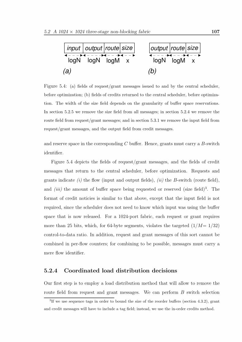
5.2 A 1024 × 1024 three-stage non-blocking fabric 107
sizeoutput route
logN logM
input
logN
sizeoutput route
logN logM
(b)(a)x x
Figure 5.4: (a) fields of request/grant messages issued to and by the central scheduler,
before optimization; (b) fields of credits returned to the central scheduler, before optimiza-
tion. The width of the size field depends on the granularity of buffer space reservations.
In section 5.2.5 we remove the size field from all messages; in section 5.2.4 we remove the
route field from request/grant messages; and in section 5.3.1 we remove the input field from
request/grant messages, and the output field from credit messages.
and reserve space in the corresponding C buffer. Hence, grants must carry a B-switch
identifier.
Figure 5.4 depicts the fields of request/grant messages, and the fields of credit
messages that return to the central scheduler, before optimization. Requests and
grants indicate (i) the flow (input and output fields), (ii) the B-switch (route field),
and (iii) the amount of buffer space being requested or reserved (size field)3. The
format of credit noticies is similar to that above, except that the input field is not
required, since the scheduler does not need to know which input was using the buffer
space that is now released. For a 1024-port fabric, each request or grant requires
more than 25 bits, which, for 64-byte segments, violates the targeted (1/M= 1/32)
control-to-data ratio. In addition, request and grant messages of this sort cannot be
combined in per-flow counters; for combining to be possible, messages must carry a
mere flow identifier.
5.2.4 Coordinated load distribution decisions
Our first step is to employ a load distribution method that will allow to remove the
route field from request and grant messages. We can perform B switch selection
3If we use sequence tags in order to bound the size of the reorder buffers (section 4.3.2), grant
and credit messages will have to include a tag field; instead, we use the in-order credits method.

108 Chapter 5 A Non-Blocking Benes Fabric with 1024 Ports
using per-flow round-robin segment distribution4. Besides other advantages discussed
in section 4.2.3, this distribution method ensures that the route of each segment
can be independently and consistently determined at both its (per-output) credit
scheduler, and at its ingress linecard. Thus, this route assignment does not have to
be communicated from the scheduler to the ingress linecard: upon receiving a grant,
the linecard can infer the route assigned to the segment by the credit scheduler. To
do so, both of those units initialize a private, per-flow pointer to an agreed upon B
switch, and then advance that pointer for every new grant or segment of that flow.
In this way, we reduce the request/grant width by log2 M bits, each. (Observe that
credits still need the route field.)
By removing the route field, it is now possible to combine the per-flow requests and
grants in per-flow request and grant counters, respectively: each such counter counts
the number of requested or granted bytes corresponding to a given flow. However,
there is a final subtle issue that we need to take care of. A grant counter maintains the
cummulative amount of buffer space reserved for a given flow, thus it does not prevent
consecutive grants from being merged with each other. This merging is not permitted
if grants have variable size, since, due to multipath routing, contiguous grants issued
to a given flow correspond to buffer spaces in different crosspoint queues.
We circumvent this intricancy by eliminating the size field from requests and
grants. This is trivial when the system operates on fixed-size packets (cells). The
following subsection shows that we can achieve the same for variable-size segments, by
making each request-grant transaction always refering to a maximum-size segment.
5.2.5 Buffer reservations: fixed or variable space?
To support variable-size segments, one has the option of either (i) having each request-
grant transaction explicitly specify a size and carry the corresponding count; or (ii)
always request and allocate buffer space for a maximum-size segment, even when
the real segment that will eventually travel through that space is of a smaller size.
We opt for fixed size allocation, for simplicity reasons: in this way, we reduce the
4This method ignores the (usually small) load imbalance caused by the varying segment size.

5.2 A 1024 × 1024 three-stage non-blocking fabric 109
width of requests and grants and the width of credits returned from C switches (these
messages do not need to carry a size field); the width of the credit counters maintained
by the credit schedulers is also reduced. But most imprortantly, this method allows
merging consequtive requests and grants into per-flow counters (with a small width
each5). Request counters maintain the number of maximum-size segments requested
by a given flow; and grant counters maintain the number of maximum-size segments
granted to a given flow.
A disadvantage of this method becomes apparent when the arriving packets have
small size. Then, some segments may not be full, and buffer space can be underuti-
lized. But this problem is valid only for light flows, and with such light flows, it may
not be a problem to underutilize some buffer space; if a flow persists, its VOQ will
grow, and segments will start having full size –see variable-size multi-packet segments
[Katevenis05], also described in section 2.1.1.
Having obviated the need for route and size fields, request/grant messages only
convey a flow identifier. Section 5.3.1 shows how, by using time division multiplexing,
each flow identifier can be encoded in log2 N bits when being conveyed to and from
the central scheduler, instead of the 2 · log2 N bits that would normally be required.
Before going into that, we review the operations in the system.
5.2.6 Operation overview
The segments injected into the fabric have size greater than or equal to a given
minimum packet size , MinP 6. All control schedulers operate at the rate of such
minimum-size packets, i.e. one new decision per MinP time. We could instead make
5If requests referred to a different number of bytes each, we would have to maintain a queue
of request sizes, rather than a mere total-bytes count. If we only a had a total-bytes count, the
problem would be the following: At grant time, we do not know the size of the packet to grant for;
if we grant for a maximum-size packet, and the input uses a portion of the granted bytes, then what
should happen to the rest of the granted bytes, which correspond to a portion of the next packet,
and cannot be discarded because no new grant will ever be issued for precisely those same bytes?6We do not want smaller segments, so that the rate of fabric schedulers can be kept ≥ than the
rate of minimum-size packets, without needlessly letting links idle.

110 Chapter 5 A Non-Blocking Benes Fabric with 1024 Ports
them operate at the rate of maximum-size segments, taking advantage of the fact that,
if the scheduling rate does not suffice to drain VOQs fast enough, VOQs will grow,
and the injected segments will become full. This would relax timing constraints and
simplify the design; the targeted control-to-data ratio would also be easier to achieve.
However, even if the scheduling rate fails to drain the aggregate VOQ load, some
VOQs may still not contain full size segments. For example, when a few VOQs carry
a high percentage of the incoming load, the remaining VOQs will almost always be
empty, as they will get served by the time they become active. Under these condi-
tions, the schedulers may frequently serve non-full segments, thus wasting scheduling
bandwidth, while heavy VOQs continue to grow.
Limiting the per-flow outstanding requests
Each ingress linecard limits the number of requests that a VOQ may have outstanding
inside the central scheduler to an upper bound u. This has the following benefits.
First, the respective request or grant counter in the central scheduler will never wrap
around (overflow) if it is at least dlog2ue-bit wide. Second, this “flow control” equalizes
a flow’s request with its grant rate, and prevents output credit schedulers from severely
synchronizing in conflicting decisions, i.e. granting buffers to a few, oversubscribed
inputs (see section 3.5.2).
Segment admission
Each linecard maintains two variables, pending requests (pr) and received grants (rg),
for every corresponding VOQ. Initially, both variables are set to zero (0); on every
(per-VOQ) request sent, pr is incremented by one; on every (per-VOQ) grant received,
pr is decremented by one, and rg is incremented by one. Finally, rg is decremented
by one when a (per-VOQ) new segment is forwarded into the fabric. The forwarding
of a new VOQ request is subject to the following two conditions: (i) pr < u; and
(ii) (pr + rg) × maximum-segment-size < VOQ-length. A request scheduler visits
the VOQs for which both conditions (i) and (ii) hold, and sends requests for the
corresponding outputs to the central scheduler, at the rate of one request per input,

5.2 A 1024 × 1024 three-stage non-blocking fabric 111
per MinP -time.
Upon reaching the central scheduler, each request, say i→o, increments the i→o
request count, which is maintained in front of the credit scheduler for output o. Every
output’s credit scheduler also maintains M credit counters, one per crosspoint queue
in its C switch, and N distribution pointers, one per flow arriving to this output. Each
credit counter is decremented by one when the credit scheduler allocates space from
that counter to one segment. Each distribution pointer identifies the B switch through
which to route the next segment of the corresponding flow, i→o; it is initialized and
incremented as described in section 5.2.4. Flow i→o is eligible for service at its
(output) credit scheduler when its request counter is non-zero and the credit counter
pointed by the distribution counter i→o is also non-zero. Once flow i→o gets served,
its request count is decremented by one, and a grant is routed to its input grant
scheduler, where it increments grant counter i→o by one. Any non-zero grant counter
is always eligible for service, and, once served, is decremented by one. When served,
grant i→o is sent to its ingress linecard, to admit a new segment inside the fabric.
Segment injection
As mentioned, when the grant arrives to linecard i, the rg variable for VOQ i→o is
incremented by one, and the queue is ready to inject its head segment into the fabric.
One segment is injected even if its size is not the maximum (grants always refer to
maximum-size segments). The reason why VOQ i→o does not contain a maximum-
size segment is that this smaller segment is the only datum in the queue at the time
of injection7. The route of the injected segment is given by input distribution counter
i→o; this counter is initialized and incremented as described in section 5.2.4. Before
injecting a segment, a sequence tag is appended in its header, specifying its order
among other segments in flow i→o. Sequence tags are used by the reordering logic in
egress linecards.
7Actually, a segment with size smaller than the maximum will also be injected when dispatching
a full size segment leaves the queue with data of size < MinP , in which case, the queue may later
have to inject a segment of size smaller than MinP .

112 Chapter 5 A Non-Blocking Benes Fabric with 1024 Ports
S
S
S
S
S
cros
spoi
nts
S
S
cros
spoi
nts
cros
spoi
nts
A1 C1
C2 B2A2B2
VOQ
s cred. cred. cred.
(ingr
ess)
(egr
ess)
B1linecard 1
linecard2 linecard2
linecard 1
Reas
sem
bly
Reor
der &
Figure 5.5: Datapath of a 4 × 4 fabric. Credits are sent upstream at the rate of one
credit per minimum-segment time, and convey the exact size of the buffer space released,
measured in bytes.
Observe that segment injection is subject to “local” backpressure exerted from
the crosspoint buffers inside the downstream A-switch, and thus it may not be pos-
sible at the time when the grant arrives. A link scheduler in each linecard forwards
segments from VOQs with rg > 0, subject to the availability of A-stage credits. The
segment has then to compete against other granted segments, and will reach its C
switch subject to hop-by-hop (“local”) backpressure. The datapath and the internal
backpressure of the fabric are depicted in Fig. 5.5. The intra-fabric (local) backpres-
sure is indiscriminate (not per-flow), but, as explained in section 4.2.3, it does not
introduce harmful blocking.
Note that our system also uses backpressure from the C stage to the B stage,
so as to allow a few segments to be injected without having first secured end-to-end
credits –see section 2.2.2. When all injected segments have been granted credits, this
backpressure will never be activated, since buffer space in stage C is reserved by the
request-grant scheduled backpressure. No “local” backpressure is needed from the
egress linecards to the C stage.
Segment resequencing & packet reassembly
When the segment reaches its egress linecard, the resequencing logic gets activated
–see Fig. 5.6. If the segment is in-order (with regard to other segments in the same

5.2 A 1024 × 1024 three-stage non-blocking fabric 113
in1in2
space: N*MxP
buffer bufferreorder packet reassembly
fabricin−order pcksegmentssegments
early packet
space: B per−inputqueues
final
outputS
inN45
5 4 2 1
8 7
Figure 5.6: The egress linecard contains per-flow queues, in order to perform segment
resequencing and packet reassembly.
flow), it is immediately handed to the packet reassembly unit. Out-of-order segments
have to wait inside the reorder buffer until the late segment(s) arrive8. For each
in-order segment, a credit is sent to the central scheduler. This credit notifies the
corresponding credit scheduler that the buffer space reserved for the segment is avail-
able again. (A segment may pull out of the reorder buffer several “early” segments
the same flow, and, thus, it may trigger the departure of multiple credits towards the
control scheduler9.) The packet reassembly unit extracts packet fragments from seg-
ments, and glues them together to form complete packets. An output link scheduler
forwards complete packets to the final output.
5.2.7 Data round-trip time
As shown in Fig. 5.7, the data round-trip time (RTT), used in sizing crosspoint
buffers, spans from the beginning of a credit scheduling operation that reserves a
credit, to the time that credit returns back to the central scheduler. It consists of
credit and grant scheduler delays plus grant sojourn time from scheduler to ingress
plus segment sojourn time from ingress to egress plus credit sojourn time from egress
linecard to scheduler (Fig. 5.2: arrows 2, 3, and 4). Observe that we measure the
8The reorder buffer and the reassembly buffer can be implemented inside a common physical
memory: no memory-copy operation is needed in order to move a segment from one buffer to the
other.9Credits are sent at the rate of one credit per MinP -time, per egress.

114 Chapter 5 A Non-Blocking Benes Fabric with 1024 Ports
Sinput 2grant SSS SScredit
output 1 creditreturn
Screditoutput 1
Sinput 2grantScredit
output 1SSS S
ingress A−st. B−st. C−st.
creditreturn
round−trip time
ingress A−st. B−st. C−st.MinPtime
reorder
reorderbuffer
buffer
Figure 5.7: The control (data) round-trip time; the delay of each scheduling operation is
one MinP -time.
RTT assuming that no contention is present, and thus with zero queueing delay.
The minimum segment delay is approximately equal to the data round-trip time.
It does not include the credit sojourn time from the egress linecard to the control
scheduler, but it includes the request travel time from the ingress linecard to the
control scheduler.
5.3 Central scheduler implementation
In this section we estimate the area and the I/O bandwidth of the central scheduling
chip. We start by showing how time division multiplexing (TDM) can reduce the size
of request (and grant) messages that are sent to and from the central scheduler.
5.3.1 TDM communication with central scheduler
Each linecard issues one VOQ request and receives one grant per MinP time. As
shown in Fig. 5.8, linecard requests travel through their corresponding A-switch, and
scheduler grants travel through their corresponding C-switch. On the links connecting
linecards to A-switches, requests carry an identifier of the output port they refer to.
Inside the A-switch, the requests from the M upstream linecards are time-division
multiplexed on a link that transfers M (equal to TDM frame size) requests to the
scheduler per MinP time, one from each linecard. The scheduler infers the ingress

5.3 Central scheduler implementation 115
in M
in 1in 2
linecards
outp
id
outp
id
outp
id
sche
dulin
g
in1in2
inM
switchC
in M
in 1in 2
outp
id
outp
id
outp
id
TDM frame
switchA
1 2 M
grantsfor linecards
TDM frameinMin2in1
requestsfrom
21 M
central scheduler
Figure 5.8: Request-grant communication with the central scheduler using time division
multiplexing (TDM). A single physical linecard serves both ingress and egress functions;
in the ingress path each linecard has an outgoing connection to an A-switch; in the egress
path, each linecard has an incoming connection from a C-switch.
port of a request from its position in the TDM frame. Similarly, the grants issued for
linecards of a particular C-switch10 depart from the scheduler on a TDM link: the
position (slot) of a grant in the TDM frame indicates the linecard that must receive
each grant.
The payload of each request or grant notice is an identifier of the fabric-output
port that the notice goes to or comes from; this destination identifier can be encoded
in log2N bits11. (The input identifier is encoded “in time”.) Besides request-grant
notices, the central scheduler must also receive credits from the switches in the C
stage. These credits are conveyed through a link connecting each C-switch with the
scheduler. Each such link carries M credits per MinP time, one per output port,
in a similar TDM manner: the position of a credit in the TDM frame identifies the
output port that the credit comes from, and its payload specifies the crosspoint queue
in front of that port that generated the credit –i.e. log2 M bits payload per TDM
slot.
10Each physical linecard serves both ingress and egress functions; therefore, the grants can be
routed to ingress linecards through the C-switches.11More accurately, we need log2(N + 1) bits, in order to be able encode idle TDM slots.

116 Chapter 5 A Non-Blocking Benes Fabric with 1024 Ports
inp 1 inp 2 inp 3 inp 4 inp 1 inp 2 inp 3 inp 4
cnt
cnt
cnt
cnt
cnt
cnt
cnt
cnt
cnt
cnt
cnt
cnt
cnt
cnt
cnt
cnt cnt
cnt cnt cnt
cnt
cnt
cnt
cnt cnt cntcnt
cnt cnt cntcnt
grant
(demux)
schedulers (mux)
(mux)
(demux)
inpu
t 4
inpu
t 1
inpu
t 2
inpu
t 3cn
t
request counters grant counters
creditschedulers
ingress linecards
pipelined, single−resource, credit and grant schedulers
A1 A2 C1 C2
outp 1
outp 2
outp 3
outp 4
inp 1 inp 2 inp 3 inp 4
Figure 5.9: The internal organization of the central scheduler for N= 4 and M= 2. There
are N2 request counters, and N 2 grant counters. Not shown in the figure are the N 2 flow
distribution pointers and the N ·M credit counters.
5.3.2 Scheduler chip bandwidth
Using TDM multiplexing, the aggregate bandwidth of the scheduler’s chip is 2 · N ·
log2 N bits per MinP time –for receiving requests from and issuing grants to all
fabric-input ports– plus N · log2 M bits per MinP time for receiving credits from all
fabric-outputs, for a total of N · (2 · log2 N + log2 M) bits per MinP time. For a
1024-port fabric (M= 32), with λ= 10 Gb/s and MinP= 64 Bytes, the aggregate
input plus output bandwidth is 25.6 Kbit per 51.2 ns, or roughly equal to 500 Gb/s.
5.3.3 Routing requests and grants to their queues
Figure 5.9 depicts the internal organization of the central scheduler. Requests from

5.4 Performance simulation results 117
different ingress ports arriving through a given A-switch are conceptually demulti-
plexed and routed to their (output) credit scheduler. (In an actual implementation,
no demultiplexing is needed, and the counters can be held in SRAM blocks, accessed
in the same TDM manner as external links.) At the interface of the scheduler’s chip,
we have N inputs that want to talk to N output schedulers. As shown in Fig. 5.9,
this can be implemented by a crossbar. Each crossbar input needs only identify the
output for which it has a new request –no other payload is being exchanged. When
a credit (output) scheduler (middle of the chip) serves an input, it increments by one
the corresponding grant counter (right half of the chip). The grant counters form
another conceptual “crossbar” analogous to the one formed by the request counters.
Transistor counts
This first, conceptual organization uses 2·N 2 request/grant counters, dlog2ue-bit wide
each, and N2, log2M -bit wide, distribution (load balancing) counters. For a 1024-
port fabric, and u= 32, this results in roughly 15 M of counter bits. Assuming that
each such bit costs about 25 transistors, the chip that used such a straightforward
implementation would need approximately 375 M transistors, in total.
A better implementation groups several counters in sets, implemented as SRAM
blocks with external adders for increments and decrements. In this way, we can
reduce the chip die considerably, since SRAM is much more compact than random
logic. At the same time, input or output operations are time multiplexed on a set of
hardware controllers running faster than the MinP time. For instance, we can group
outputs in groups of M , and use only one credit scheduler controller performing
request admissions for these outputs, in a TDM manner.
5.4 Performance simulation results
We used simulations in order to verify the design and evaluate its performance for
various fabric sizes, crosspoint buffer sizes, and round-trip times. All experiments
except those in section 5.4.6 use fixed-size cell traffic, in order to compare our archi-

118 Chapter 5 A Non-Blocking Benes Fabric with 1024 Ports
tecture to alternative ones that only work with fixed-size cells. When operating on
cells, each segment injected into the SF fabric contains one cell.
The delay reported is the average, over all cells, of the cell’s exit time –after being
correctly ordered inside the egress resequencing buffers–, minus the cell’s birth time,
minus the request-grant cold start delay, and minus the cell’s sojourn time through
the fabric. Thus, under zero contention, the reported delay of a cell can be as small
as zero.
We simulated the fabric under uniformly-destined, diagonal, unbalanced, and
hotspot traffic patterns, for smooth (Bernoulli) and for bursty cell arrivals (see Ap-
pendix B for a description of traffic patterns). Inadmissible traffic patterns were also
used in order to examine how well our architecture can distribute input and output
port bandwidth based on sophisticated QoS criteria.
We use the name Scheduled Fabric (SF) to denote our system. SF uses no internal
speedup. The default schedulers in SF are pointer-based round-robin (RR) schedulers
throughout the fabric, the linecards, and the admission unit. The credit schedulers
implement the random-shuffle round-robin discipline, presented in section 3.7, for
better “desynchronization”. The data RTT is used to size the crosspoint buffers
of SF in all experiments except those in section 5.4.7 where crosspoint buffers have
smaller size than one RTT worth of traffic. The limit of outstanding requests per
VOQ, u, is set to 32.
We compare SF to output queueing (OQ), to iSLIP, and to a three-stage Clos
fabric consisting of a bufferless middle stage, and buffered first and last stages (MSM),
scheduled using the CRRD algorithm [Oki02].
5.4.1 Throughput: comparisons with MSM
First, we measure throughput for different crosspoint buffer sizes and for different
RTTs under unbalanced, smooth traffic; for comparison, we also plot the results of
MSM using 4 iterations. Observe that parameter b is the size of crosspoint buffers
measured in cells, and that the RTT refers to the (global) data round-trip time as

5.4 Performance simulation results 119
unbalance factor, w unbalance factor, w
norm
aliz
ed th
roug
hput
SF
4 iterationsSF 64 ports
MSM 256 ports
MSM 64 ports4 iterations
b12−rtt0
b4−rtt0b8−rtt0
b16−rtt16 (64 ports)
b12−rtt12b12−rtt6
b12−rtt12(64, 144, and 256 ports)
(a) (b) 0 0.2 0.4 0.6 0.8 1 0 0.2 0.4 0.6 0.8 1
0.6 .65 0.7
.75 0.8
.85 0.9
.95 1.0
Figure 5.10: Throughput under unbalanced traffic; fixed-size cell Bernoulli arrivals; 100%
input load. (a) 64-port fabric (N= 64, M= 8); (b) varying fabric sizes up to N= 256, M=
16.
defined in section 5.2.7. Figure 5.10(a) shows that with b as small as 12 cells, SF
approaches 100% throughput under uniformly-destined traffic (w= 0), and provides
more than 95% throughput for intermediate w values, which correspond to unbalanced
loads. We also see that, with the same buffer size (b= 12), and for any RTT up to 12
cell times, this performance does not change. Figure 5.10(b) shows this performance
to stay virtually unaffected by the fabric size, N , when the latter changes from 64
to 256. By contrast, the performance of MSM drops sharply with increasing N .
Although MSM may deliver 100% throughput (similar to iSLIP), it is designed to do
that for the uniform case, when all VOQs are persistent: when some VOQs fluctuate,
pointers can get synchronized, thus directly wasting output slots. By contrast, SF
does not fully eliminate packet conflicts; in this way, every injected cell, even if
conflicting, makes a step closer to its output, thus being able to occupy it on the first
occasion.
With b= 12 cells, the size of the reorder buffer inside each egress linecard is 12 ·M
cells; for 64-byte cells, this reorder buffer space is 6 KBytes in a 64× 64 system, 12
KBytes in a 256× 256 system, and 24 KBytes in a 1024× 1024 system.
5.4.2 Smooth arrivals: comparison with OQ, iSLIP, and MSM

120 Chapter 5 A Non-Blocking Benes Fabric with 1024 Ports
Scheduled Fabric
64 ports
256 ports
normalized input load
OQ
(ports 64, 144, and 256)
2−SLIP
aver
age
dela
y (c
ell t
imes
)
4 iterationsMSM
0.1
1
10
100
1000
0.1
1
10
100
1000
0.5 0.6 0.7 0.8 0.9 1 0.4
Figure 5.11: Delay versus input load, for varying fabric sizes, N ; buffer size b= 12 cells,
RTT= 12 cell times. Uniformly-destined fixed-size cell Bernoulli arrivals. Only the queueing
delay is shown, excluding all other fixed delays.
Figure 5.11 shows the delay-throughput performance of SF under uniformly-
destined, smooth traffic, and compares it to that of MSM, iSLIP, and ideal OQ switch.
Compared to the bufferless architectures, SF delivers much better performance. The
delay of SF is not affected by fabric size, while that of MSM increases with increasing
fabric size. The delay of SF under smooth cell arrivals is within four times that of
OQ. We hypothesize that the main source of additional delay in SF relative to OQ is
the large number of contention points that a cell goes through during its trip inside
the fabric.
5.4.3 Overloaded outputs & bursty traffic
A major concern in multistage fabrics is the adverse effect that congestion at certain
outputs may have on other uncongested outputs. Our design explicitly guards against
that danger. Figure 5.12 presents the delay of uncongested flows (non-hotspot traffic),
in the presence of a varying number of other congested outputs (hotspots). All flows,

5.4 Performance simulation results 121
OQ
normalized load at non−hotspot destinations
h/50
h/16
h/0 (uniform)h/4
aver
age
dela
y of
cel
ls d
estin
ed
to n
on−h
otsp
ots
(cel
l tim
es)
MSM (4 iterations)h/32 uniform
1 0.2 0.3 0.4 0.5 0.6 0.7 0.8 0.9 0.1
1
10
100
1000
0.1
Figure 5.12: Delay of well-behaved flows in the presence of hotspots. h/• specifies the
number of hotspots, e.g., h/4 corresponds to four hotspots. Fixed-size cell Bernoulli arrivals;
64-port fabric, b= 12 cells, RTT= 12 cell times. Only the queueing delay is shown, excluding
all other fixed delays.
congested or not, are fed by Bernoulli sources. For comparison, we also plot cell delay
when no hotspot is present, denoted by h/0, and the OQ delay.
To see how well SF isolates flows, observe that the delay of h/4 –i.e. the delay of
well-behaved flows in the presence of four (4) congested outputs– is virtually identical
to that of h/0. Nevertheless, the delay of well-behaved flows is increasing with the
number of hotspots, with the increase being more pronounced for large numbers of
hotspots. If the well-behaved flows were subject to backpressure signals coming from
queues that feed oversubscribed outputs, these flows’ delay would probably grow
without bound, even at very moderate loads. However, this is not the case with SF.
The observed increase in delay is not due to congestion effects, but to hotspot traffic
increasing the contention along the shared paths inside the fabric. For instance, when
fifty out of the sixty-four output ports of the fabric are oversubscribed (h/50), and
the load of the remaining fourteen output flows is 0.1, the effective load at which
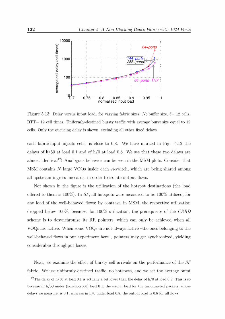
122 Chapter 5 A Non-Blocking Benes Fabric with 1024 Ports
0.7 0.75 0.8 0.85 0.9 0.95 1normalized input load
144−ports256−ports
10
100
1000
10000
aver
age
cell
dela
y (c
ell t
imes
)
64−ports
64−ports−TH7
Figure 5.13: Delay versus input load, for varying fabric sizes, N ; buffer size, b= 12 cells,
RTT= 12 cell times. Uniformly-destined bursty traffic with average burst size equal to 12
cells. Only the queueing delay is shown, excluding all other fixed delays.
each fabric-input injects cells, is close to 0.8. We have marked in Fig. 5.12 the
delays of h/50 at load 0.1 and of h/0 at load 0.8. We see that these two delays are
almost identical12! Analogous behavior can be seen in the MSM plots. Consider that
MSM contains N large VOQs inside each A-switch, which are being shared among
all upstream ingress linecards, in order to isolate output flows.
Not shown in the figure is the utilization of the hotspot destinations (the load
offered to them is 100%). In SF, all hotspots were measured to be 100% utilized, for
any load of the well-behaved flows; by contrast, in MSM, the respective utilization
dropped below 100%, because, for 100% utilization, the prerequisite of the CRRD
scheme is to desynchronize its RR pointers, which can only be achieved when all
VOQs are active. When some VOQs are not always active –the ones belonging to the
well-behaved flows in our experiment here–, pointers may get synchronized, yielding
considerable throughput losses.
Next, we examine the effect of bursty cell arrivals on the performance of the SF
fabric. We use uniformly-destined traffic, no hotspots, and we set the average burst
12The delay of h/50 at load 0.1 is actually a bit lower than the delay of h/0 at load 0.8. This is so
because in h/50 under (non-hotspot) load 0.1, the output load for the uncongested packets, whose
delays we measure, is 0.1, whereas in h/0 under load 0.8, the output load is 0.8 for all flows.
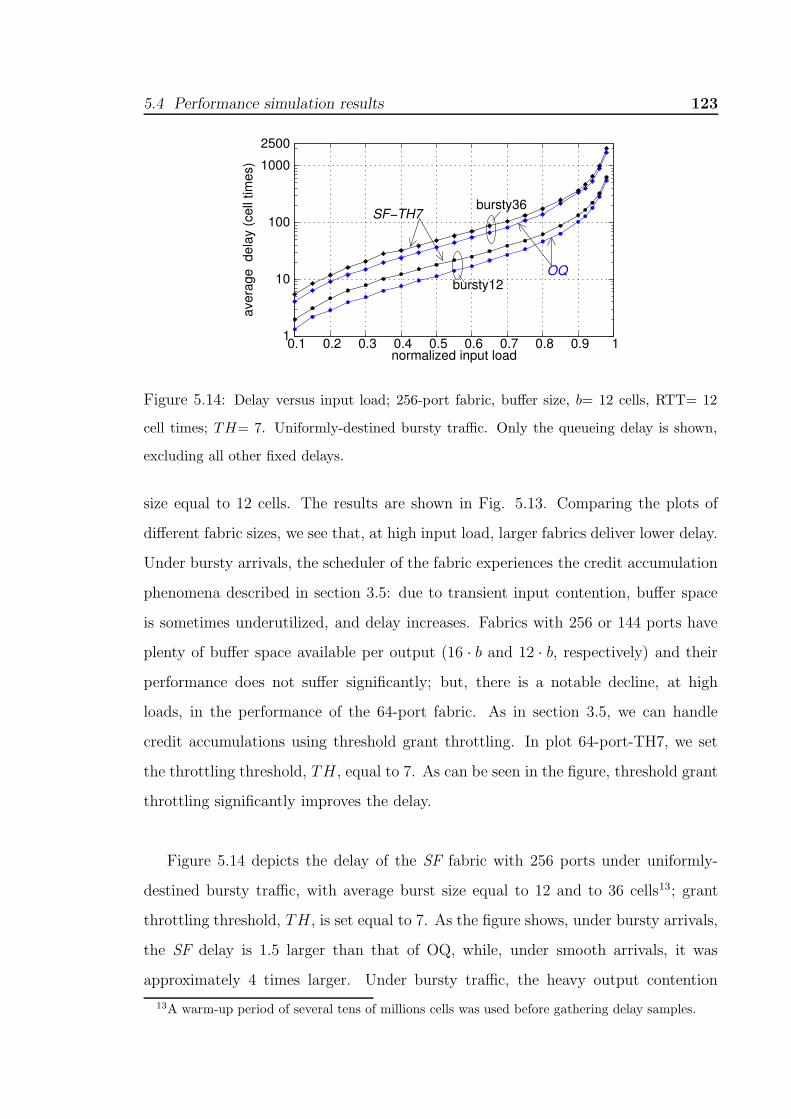
5.4 Performance simulation results 123
bursty12OQ
bursty36SF−TH7
0.1 0.2 0.3 0.4 0.5 0.6 0.7 0.8 0.9 1normalized input load
aver
age
del
ay (c
ell t
imes
)
1
10
100
1000
2500
Figure 5.14: Delay versus input load; 256-port fabric, buffer size, b= 12 cells, RTT= 12
cell times; TH= 7. Uniformly-destined bursty traffic. Only the queueing delay is shown,
excluding all other fixed delays.
size equal to 12 cells. The results are shown in Fig. 5.13. Comparing the plots of
different fabric sizes, we see that, at high input load, larger fabrics deliver lower delay.
Under bursty arrivals, the scheduler of the fabric experiences the credit accumulation
phenomena described in section 3.5: due to transient input contention, buffer space
is sometimes underutilized, and delay increases. Fabrics with 256 or 144 ports have
plenty of buffer space available per output (16 · b and 12 · b, respectively) and their
performance does not suffer significantly; but, there is a notable decline, at high
loads, in the performance of the 64-port fabric. As in section 3.5, we can handle
credit accumulations using threshold grant throttling. In plot 64-port-TH7, we set
the throttling threshold, TH, equal to 7. As can be seen in the figure, threshold grant
throttling significantly improves the delay.
Figure 5.14 depicts the delay of the SF fabric with 256 ports under uniformly-
destined bursty traffic, with average burst size equal to 12 and to 36 cells13; grant
throttling threshold, TH, is set equal to 7. As the figure shows, under bursty arrivals,
the SF delay is 1.5 larger than that of OQ, while, under smooth arrivals, it was
approximately 4 times larger. Under bursty traffic, the heavy output contention
13A warm-up period of several tens of millions cells was used before gathering delay samples.

124 Chapter 5 A Non-Blocking Benes Fabric with 1024 Ports
bursty 12
bursty 36
aver
age
dela
y of
cel
ls d
estin
ed
to n
on−h
otsp
ots
(cel
l−tim
es)
OQ
SF: h/16SF: h/4
SF: uniform
1 0.1 0.2 0.3 0.4 0.5 0.6 0.7 0.8 0.9 1normalized load at non−hotspot destinations
10
100
1000 2000
Figure 5.15: Delay of well-behaved flows in the presence of hotspots, for varying burstiness
factors. Bursty fixed-size cell arrivals; 256-port fabric, b= 12 cells, RTT= 12 cell times.
Only the queueing delay is shown, excluding all other fixed delays.
masks out the small delays at the internal contention points of the SF fabric. The
same performance trends can be found in [Sapunjis05].
In the following experiment we evaluate the performance of SF (256 ports), with no
threshold grant throttling, under bursty cell arrivals and 0, 4, and 16 hotspots; thresh-
old grant throttling gives even better results than those that we present here. For
comparison we also plot the performance of the output queueing switch. The results
are shown in Fig. 5.15. As can be seen, the presence of hotspots does not affect the
delay of well-behaved flows. In most non-blocking fabrics, the primary source of delay
under bursty arrivals is the severe (temporal) contention for the destination ports,
many of which may receive parallel bursts from multiple inputs [Li92][McKeown99a].
For the same reason, under the bursty model, the incremental delay that well-behaved
flows experience in the presence of hotspots is less pronounced than with Bernoulli
arrivals –Fig. 5.15 versus Fig. 5.12.

5.4 Performance simulation results 125
conn
ectio
ns’ r
ate
utiliz
atio
n of
out
put 1
connections’ load
2−>1 (weight: 9)
9−>1 (weight: 1)
1−>1 (weight: 20)
(other outputs 90% loaded with bursty traffic)
0.2
0.4
0.6
0.8
0.1 0.2 0.3 0.4 0.5 0.6 0.7 0.8 0.9 1
1.0
0 0
Figure 5.16: Sophisticated output bandwidth allocation, using WRR/WFQ credit sched-
ulers; 64-port fabric, b= 12 cells, RTT=12 cell times.
5.4.4 Weighted round-robin output port bandwidth reserva-
tion
The SF architecture not only protects one output flow from another, but can also
differentiate among flows going to the same output, if so desired for QoS purposes.
Previous experiments used RR schedulers. Now, we modify the (single-resource)
credit schedulers, which allocate output-port bandwidth to competing inputs: in this
experiment we use WRR/WFQ credit schedulers14 .
In Fig. 5.16, we configured three flows (connections) in a 64-port fabric, flows
1→1, 2→1, and 9→1, with weights of twenty (20), nine (9), and one (1), respectively;
each of them is the only flow active at its input, and the load it receives changes along
the horizontal axis. Inputs other than 1, 2, and 9, receive a uniformly-destined bursty
(background) traffic, at 0.9 load, targeting outputs 2 to 64. The vertical axis depicts
connections’ normalized service (rate), measured as cell rate at the output ports of
the fabric.
As Fig. 5.16 shows, when the demand for output 1 is feasible (up to 0.33 load per
14All other schedulers within the fabric are left intact (RR).

126 Chapter 5 A Non-Blocking Benes Fabric with 1024 Ports
flow), all flows’ demands are satisfied. At the other end, when all flows are saturated
(starting from 0.66 load per flow), each flow gets served at a rate equal to its fair
share –i.e. 0.66, 0.30, and 0.033. When the load of a flow is below this fair share,
the bandwidth that stays unused by this flow gets distributed to the other flows, in
proportion to those other flows’ weights.
5.4.5 Weighted max-min fair schedules
In this section, in addition to the WRR (output) credit schedulers that we had in
section 5.4.4, we also use WRR (input) request schedulers. Each VOQ flow i→j has
a unique weight; this weight is being used by the WRR request scheduler at ingress
i, as well as by the WRR credit scheduler for output port j. We model persistent
VOQs –either continuously full or continuously empty– and we measure the rate of
their flows. Each active VOQ is fed with back-to-back cells arriving at line rate. The
outstanding request threshold, u, is set equal to 32, thus the request rate of a VOQ
connection gets equalized to its grant (service) rate (see section 5.2.6).
First, we configure a “chain” of dependent flows as in [Chrysos02]. The left table
in Fig. 5.17(a) depicts flow weights in a 4×4 fabric made of 2×2 switches. When flow
1→1 is active, with a weight of 64, its weighted max-min fair (WMMF) share is 2/3,
and each subsequent connection along the diagonal of the table deserves a WMMF
rate of 1/3, 2/3, 1/3, etc15. Service rates are shown in the table on the right (upper
corner in each box): the rates that the SF fabric assigns to connections exactly match
their WMMF shares. When 1→1 is inactive, with zero weight, the fair shares of the
remaining connections get reversed, becoming 2/3, 1/3, 2/3, etc. As shown in the
bottom corner of each box in the table, again simulation rates exactly match these
new WMM fair shares.
In Fig. 5.17(b) we configured 16 active connections in the 4-port fabric; their
weights, their WMMF shares, as well as the SF simulated rates are shown in the
tables. We again see that the rate allocation produced by the SF fabric approximates
15For algorithms computing WMM fair schedules refer to [Hahne91].

5.4 Performance simulation results 127
1
4
4
4
1
3
2 1
3
2
2
1
1
1
1 1
(a)
(b)
32
16 8
4 2
1
0
.266 .383 .158 .191
.246.367.122.266
.266 .208 .316 .208
.354.158.2860.20.2 .289 .154
.20
.344
.318
.366 .244
.191.156.384
.122.267
.267
064 .667 .333
.667 .333
.667 .333
.667
.667
.333 .667
.333 .667
.333
flow weights simulated rates
flow weights
.268 .201
simulated vs.
in3
in4
in2
in1
out1 out2 out3 out4
in1
in2
in3
in4
out1 out2 out3 out4
WMM fair rates
Figure 5.17: Weighted max-min fair allocation of input and output port bandwidth, using
WRR/WFQ schedulers; 4-port fabric, b= 12 cells, RTT=12 cell times.
very close the ideal WMM fair allocation. To the best of our knowledge, this is the first
time that distributed scheduling has been shown to produce WMM fair allocations
in three-stage fabrics with shared queues.
5.4.6 Variable-size multi-packet segments
Our results up to now assumed single-cell segments carrying the payload of fixed-size
cell traffic. In the following set of experiments, we present performance simulations
of variable-size multi-packet segments that carry the payload of variable-size packets.
We assume 10 Gb/s (Poisson) sources sending variable-size packets, with exponential
inter-arrival times. We use the three packet size distributions, depicted in Table 5.1:
uniform, pareto, and bimodal. In the bimodal distribution, 95% of the packets have a
size of 64 Bytes, while the remaining 5% are 1500 Bytes in size. In these experiments,
SF uses reassembly buffers inside the egress linecards, to form (or extract) complete
packets from the multi-packet segments that depart from the reorder buffer.

128 Chapter 5 A Non-Blocking Benes Fabric with 1024 Ports
Type Minimum Size Maximum size Mean size
(Bytes) (Bytes) (Bytes)
Uniform 64 1500 814
Pareto 64 1500 454
Bimodal 64 1500 135
Table 5.1: Packet size distributions.
We compare the SF architecture to a buffered crossbar with no segmentation
or reassembly (Variable Packet-Size (VPS) crossbar), similar to the architecture in
[Katevenis04]. The round-trip time in VPS is 400 ns, yielding a FC window of 500
Bytes. The buffer space per crosspoint is 2 KBytes, i.e. ≈ 1 FC window plus one max-
imum packet size. We assume cut through operation both in VOQs and in crosspoint
buffers; the minimum packet delay is 230 ns (0.23 microseconds).
For SF, the maximum and the minimum segment size is 128 Bytes and 64 Bytes,
respectively. The data round-trip time is 1224 ns, yielding a FC window of 1530
Bytes (≈ twelve (12) 128-byte segments) at 10 Gb/s. Each crosspoint queue has size,
b, equal to 1 FC window, while the size of the reorder buffers per output is M · b (12
KBytes in a 64× 64 system, and 47 KBytes in a 1024× 1024 system). The minimum
packet delay equals 1200 ns (1.2 microseconds). Request (grants) travel at the rate
of 1 request (grant) per 64-byte time, per linecard.
Figure 5.18 presents average packet delay in SF and in VPS, under uniformly-
destined packets, for the three packet size distribution of Table 5.1. At low loads,
the dominant delay factors in SF are the VOQ delay, –VOQ delay includes 600 ns of
request-grant, cold-start delay–, as well as the reordering and the reassembly delays.
Excluding the request-grant delay overhead, and neglecting the bimodal distribution
for the moment, the delay of SF is within 2 to 3 times larger than the delay of
single-stage buffered crossbars that directly operate on variable-size packets.
Under bimodal packet sizes (Fig. 5.18), SF delivers very competent performance
up to 0.98 input load; at this high load point, SF delay increases sharply. The reason
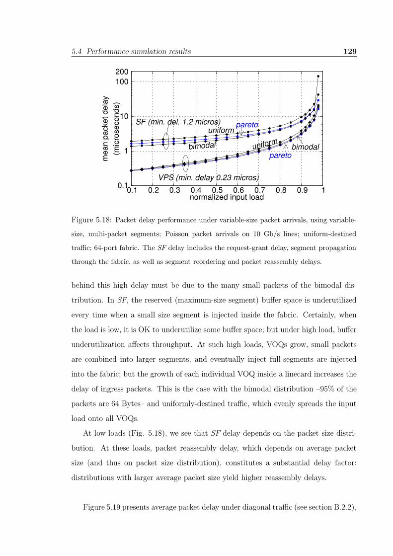
5.4 Performance simulation results 129
paretouniform
bimodal uniform
paretobimodal
VPS (min. delay 0.23 micros)
SF (min. del. 1.2 micros)
0.1 0.2 0.3 0.4 0.5 0.6 0.7 0.8 0.9 1normalized input load
0.1
1
10
100 200
mea
n pa
cket
del
ay(m
icro
seco
nds)
Figure 5.18: Packet delay performance under variable-size packet arrivals, using variable-
size, multi-packet segments; Poisson packet arrivals on 10 Gb/s lines; uniform-destined
traffic; 64-port fabric. The SF delay includes the request-grant delay, segment propagation
through the fabric, as well as segment reordering and packet reassembly delays.
behind this high delay must be due to the many small packets of the bimodal dis-
tribution. In SF, the reserved (maximum-size segment) buffer space is underutilized
every time when a small size segment is injected inside the fabric. Certainly, when
the load is low, it is OK to underutilize some buffer space; but under high load, buffer
underutilization affects throughput. At such high loads, VOQs grow, small packets
are combined into larger segments, and eventually inject full-segments are injected
into the fabric; but the growth of each individual VOQ inside a linecard increases the
delay of ingress packets. This is the case with the bimodal distribution –95% of the
packets are 64 Bytes– and uniformly-destined traffic, which evenly spreads the input
load onto all VOQs.
At low loads (Fig. 5.18), we see that SF delay depends on the packet size distri-
bution. At these loads, packet reassembly delay, which depends on average packet
size (and thus on packet size distribution), constitutes a substantial delay factor:
distributions with larger average packet size yield higher reassembly delays.
Figure 5.19 presents average packet delay under diagonal traffic (see section B.2.2),

130 Chapter 5 A Non-Blocking Benes Fabric with 1024 Ports
SF (min. del. 1.2 micros)
VPS (min. delay 0.23 micros)
uniform
uniform
bimodal
bimodal
mea
n pa
cket
del
ay(m
icro
seco
nds)
0.1 0.2 0.3 0.4 0.5 0.6 0.7 0.8 0.9 1normalized input load
0.1
1
10
100
Figure 5.19: Packet delay performance under variable-size packet arrivals, using variable-
size multi-packet segments; Poisson packet arrivals on 10 Gb/s lines; diagonal traffic distri-
bution; 64-port fabric. The SF delay includes the request-grant delay, segment propagation
through the fabric, as well as segment reordering and packet reassembly delays.
for uniform and bimodal packet size distributions. As can been seen, under this un-
balanced output distribution, VPS saturates before 0.93 input load, while SF operates
robustly up to 0.98 input load. Under diagonal traffic, the SF bimodal delay stays
low even when the load is high. Since there are only two (2) active VOQs inside
each ingress linecard, input delay is not as large as with uniformly-destined traffic (N
active VOQs per linecard).
Next, we examine performance in the presence of hotspots. In Fig. 5.20, we
present the delay of non-congested packets under 0 hotspots (uniformly-destined
traffic), 4 hotspots, and 8 hotspots. As the figure shows, well-behaved packets are
virtually unaffected by the presence of hotspots.
Figure 5.21 splits the (average) delay into its per-stage components. We see that
C-stage delay outweighs A- and B-stage delays, because C-stage resolves output
contention, whereas the other stages handle explicitly load balanced traffic. Also
observe that, the egress delay in diagram (b) is markedly lower than those in (a) and

5.4 Performance simulation results 131
uniform4 hotspots8 hotspots
SF (minimum packet delay 1.2 microseconds) 1
10
0.1 0.2 0.3 0.4 0.5 0.6 0.7 0.8 0.9 1normalized input load
100
mea
n de
lay
of p
acke
ts d
estin
edat
non
−hot
spot
s (m
icro
seco
nds)
Figure 5.20: Packet delay performance under variable-size packet arrivals, using variable-
size, multi-packet segments; Poisson packet arrivals on 10 Gb/s lines; uniform and hotspot
destination distributions; uniform packet size; 64-port fabric. The SF delay includes the
request-grant delay, segment propagation through the fabric, as well as segment reordering
and packet reassembly delays.
normalized input loadnormalized input load
(mic
rose
cond
s)av
erag
e de
lay
(a) (b) (c) normalized input load
B−stageA−stage
C−stage
egressingress ingressegress
C−stage
A−stageB−stageB−stage
A−stage
C−stage
ingress
egress
0.1 1 0.2 0.3 0.4 0.5 0.6 0.7 0.8 0.9 0.01
0.1
1
10
100
0.2 0.3 0.4 0.5 0.6 0.7 0.8 0.9 0.1 1 0.1
200
0.2 0.3 0.4 0.5 0.6 0.7 0.8 0.9 1
Figure 5.21: Per-stage fabric delays for (a) uniformly-destined traffic / uniform packet
size; (b) uniformly-destined traffic / bimodal packet size; and (c) 8-hotspot traffic / uniform
packet size; 64-port fabric. In (c), we only plot the delay of the non-congested flows.

132 Chapter 5 A Non-Blocking Benes Fabric with 1024 Ports
VPS
pareto
bimodalbimodal
uniform
SF
pareto
0.2 0.4 0.6 0.8 1unbalance factor, w
0.7
.75
0.8
.85
0.9
.95
1.0
0
norm
aliz
ed th
roug
hput
Figure 5.22: Throughput of SF under Poisson, variable-size packet arrivals, using variable-
size, multi-packet segments; unbalanced traffic distribution; 64-port fabric; 100% input
load.
in (c). This is due to the lower average packet size (bimodal vs. uniform packet size
distribution), which yields lower reassembly delay.
Finally, Fig. 5.22 presents the throughput of SF and of VPS under unbalanced
traffic, for the packet size distributions of Table 5.1. Under uniformly-destined traffic
(w= 0), SF delivers a normalized throughput around 0.98, while VPS throughput
exceeds 0.99. For the pareto and the uniform packet size distributions, SF throughput
is always above 0.95, for any w value, while the VPS throughput drops below 0.90,
when traffic is unbalanced. The SF plot for the bimodal distribution exhibits an
interesting small dip at small w values. We hypothesize that this dip is due to
many packets in the bimodal distribution having small size. At small non-zero w
values, greater than zero, flows i→j, with i6=j, have a load smaller than 1/N , thus
they frequently get served just after they become active; effectively, only one or two
packets reside in the active VOQs of these flows. When these packets have small
size (e.g. 64 Bytes), the VOQs will not inject a full-size segment, thus underutilizing
buffer space. With increasing w, these light flows contribute to a smaller fraction of

5.4 Performance simulation results 133
the total load, and the buffer space underutilization effect diminishes.
5.4.7 Sizing crosspoint buffers in systems with large RTT
The data round-trip time in the SF fabric depends on the physical packaging of the
system. A multi-terabit system, achieving the capacities of the SF fabric, may be build
using several racks, distributed in areas spanning tens of meters [Minkenberg02]; un-
der these packaging conditions, the intra-fabric delay becomes a stringent constraint.
We assume that the scheduler resides close to the switching fabric, and that signals
cover a 100 meters distance –i.e. approximately 500 ns propagation delay, assuming
speed-of-light equal to 0.2 meter/ns– to go from linecard to fabric, and vice versa.
The data round-trip time contains four (4) times this distance: grant from scheduler
to ingress, data from ingress to fabric, data from fabric to egress, and credit from
egress to scheduler. Another significant contribution to the round-trip time is due
to the serialization/deserialization (SERDES) delay, which occurs every time a signal
goes in or out of a chip; we will assume that this delay is 50 ns. The control round-trip
time in our system contains 16 chip boundary transitions: grant out of control chip,
grant in-out A chip, grant in ingress, segment out of ingress, segment in-out A, B,
and C chips, segment in egress, credit out of egress, credit in-out C chip, credit in
control chip. There are also seven (7) scheduling operations that must be accounted
in the round-trip time: credit scheduling, grant scheduling, VOQ scheduling, A, B,
and C crosspoint scheduling, and egress (credit) scheduling; we assume that each
such scheduling operation lasts for one full MinP -time, i.e. 51.2 ns at 10 Gb/s,
for MinP= 64 bytes. Under these assumptions, the overall data round-trip time
is 2000 ns (propagation) + 16× 50 ns (SERDES) + 7 × 51.2 ns (scheduling), or
approximately 3200 ns in total.
In an implementation with such a large data RTT, it may be difficult to size
each crosspoint queue with one RTT worth of space. For example, in a 1024× 1024
fabric, implementing the 1024 crosspoint queues that are needed inside each chip with
buffering capacity equal to 32000 bits (= 3200 ns× 10 bits/ns) for each queue, requires
approximately 33 Mbits of on-chip memory; despite the high density of current on-

134 Chapter 5 A Non-Blocking Benes Fabric with 1024 Ports
b = 1 RTT
b = 1/2 RTTb = 1/4 RTT
b = 1/8 RTT
.80 .82 .84 .86 .88 .90 .92 .94 .96 .98 1.0
norm
aliz
ed th
roug
hput
0 0.2 0.4 0.6 0.8 1unbalance factor, w
Figure 5.23: Throughput of SF with crosspoint buffer size smaller than one RTT worth
of traffic; unbalanced traffic distribution; fixed-size cell Bernoulli arrivals; 256-port fabric,
RTT= 64 cell times; 100% input load.
chip memory, this cost is high. Through the following experiments, we will show that
it is possible to size the crosspoint queues with less than one RTT worth of buffer
capacity. This is feasible because there are M crosspoint queues in front of each
fabric-output port, which, thanks to multipath routing, can be used by any single
connection.
In the following experiments, we set the data RTT equal to 3250 ns, as described
above, which at 10 Gb/s, and for 64-byte cells, is approximately equal to 64 cell times.
Figure 5.23 depicts the throughput of a 256× 256 SF fabric, using crosspoint buffer
sizes, b, that correspond to different fractions of the 64 cell times RTT. For simplicity,
we write “b= m· RTT”, meaning that the crosspoint buffer size is m times worth the
RTT; thus, when b= 1/2 RTT, b= 32 cells. Observe that the minimum allowable
value for b is 1/M RTT, i.e. 4 cells for the 256-port fabric (M= 16) examined in
this experiment; with b < 4 cells , the aggregate buffer space in front of each fabric-
output port will be less than the data RTT, and the system will not be able to
support persistent input-output connections. As can be seen in the figure, for b= 1,

5.4 Performance simulation results 135
1/2, and 1/4 RTT, the SF fabric delivers throughput higher than 0.95 percent under
any w value, and full throughput when w=0 (uniformly-destined traffic) or when w=
1 (persistent, non-conflicting, input-output connections). For b= 1/8 RTT, the SF
throughput drops down to 0.90 under intermediate w values.
We also have results for the minimum allowable value for b, i.e. 1/16 RTT, or 4
cells. These results show that, with b= 4 cells, the throughput of SF is approximately
0.88 when w= 0, and approximately 0.57 when w= 1. The reason why the system
fails to reach full throughput in the latter case even though one (1) full FC window
buffer (16 × 4 cells) is available in front of each fabric-output port is due to the
intra-fabric (local) backpressure from stage B to stage A. When w= 1, the total
traffic volume from each A-switch is directed to a particular C-switch. For example,
the ingress linecards connected to switch A1 target, one by one, the fabric-outputs
connected to switch C1. In this way, inside each B switch, say switch B1, there is
only one crosspoint buffer active in front of the link connecting to C1, i.e. the one
which is fed by A1. To fully utilize the fabric-outputs connected to C1, link B1→C1
(as any other B→C1 link) has to be continously busy. The only active buffer in front
of that link exerts local backpressure to A1; hence that buffer has to contain at least
one local round-trip time (between switch B1 and switch A1) worth of space16. In
our example above, b= 4 cells, whereas the B→A round-trip time is approximately
7 cell times; under these conditions, the system yields a throughput of roughly 0.57
(≈ 4/7).
Figure 5.24 depicts the delay of SF, with crosspoint buffer size smaller than the
RTT, under uniformly-destined, Bernoulli and bursty traffic patterns. Again, we see
that we can lower by four times the buffer size of SF, without significantly affecting
performance. Under bursty traffic, the maximum throughput of “b=1/8 RTT” is
just above 0.96. For RTT= 64 cell times, the buffer savings achieved through “b=
16Inverse multiplexing steers evenly the incoming traffic from each ingress linecard to M A-switch
crosspoint buffers that are fed by this linecard; hence, the long-term throughput of the ingress
linecard will not be damaged even if the size of these buffers is up to M times less than the A-to-
ingress, local round-trip time.

136 Chapter 5 A Non-Blocking Benes Fabric with 1024 Ports
bursty12
b=1/8RTT
bernoulli
4 plots for:b= 1, 1/2, 1/4, and 1/8 RTT
10
100
1000
0.1
1
0.1 0.2 0.3 0.4 0.5 0.6 0.7 0.8 0.9 1
aver
age
dela
y (c
ell t
imes
)
normalized input load
Figure 5.24: Delay of SF with crosspoint buffer size smaller than one RTT worth of traffic;
uniformly-destined traffic; 256-port fabric, RTT= 64 cell times; no grant throttling used.
Only the queueing delay is shown, excluding all other fixed delays.
1/4 RTT” are adequate. The on-chip memory required inside each switch of a 1024-
port fabric is approximately 8 Mbits, which can readily be implemented on-chip; the
reorder buffer space required inside each egress linecard is just 32 (= M) × 16 (=
64/4) cells × 64 bytes/cell, or 0.25 Mbits.

Chapter 6
Congestion Elimination in Banyan
Blocking Networks
6.1 Introduction
This chapter applies request-grant scheduled backpressure in blocking, output-
buffered banyan networks [Goke73]. Congestion management in blocking net-
works is more difficult than in non-blocking ones, like the Benes, since besides fabric-
output ports, internal links can cause congestion as well. The scheduler that we
propose in this chapter for banyan networks comprises independent single-resouce
schedulers, distributed throughout the fabric, that operate in parallel, and in pipeline.
Simulation results demonstrate that our scheduler eliminates congestion from internal
links and fabric-output ports.
6.1.1 Banyan topology
The basic banyan topology uses 2×2 switches, and has log2N stages of N/2 switches,
each; an 8× 8 example is given in Fig. 6.1. Using M ×M crossbar switches, and k
stages (M > 1, k > 1), a banyan network of N= M k ports, with Mk−1 switches per
stage, can be built.
In a banyan network, there is a unique path from every input port (source) to every
137
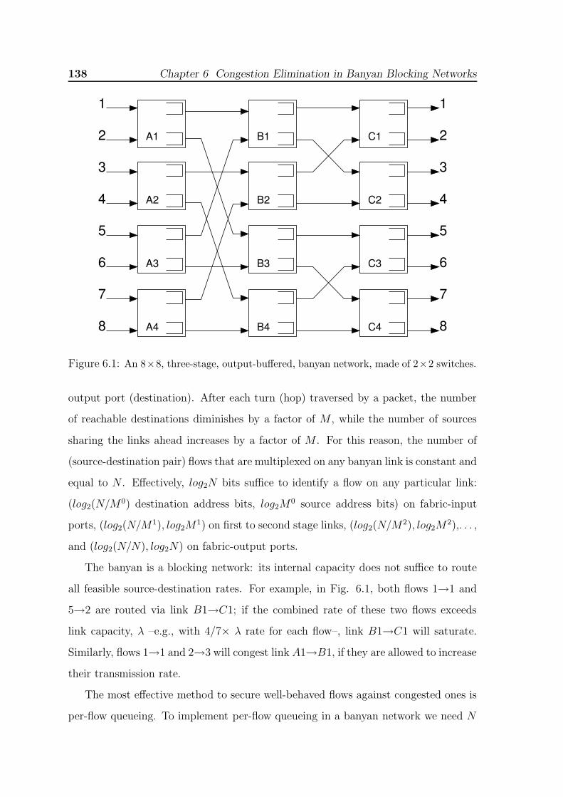
138 Chapter 6 Congestion Elimination in Banyan Blocking Networks
2 A1
1
6
3
4
5
7
8
1
2
3
4
5
6
7
8
A2
A3
A4
B1
B2
B3
B4
C1
C2
C3
C4
Figure 6.1: An 8×8, three-stage, output-buffered, banyan network, made of 2×2 switches.
output port (destination). After each turn (hop) traversed by a packet, the number
of reachable destinations diminishes by a factor of M , while the number of sources
sharing the links ahead increases by a factor of M . For this reason, the number of
(source-destination pair) flows that are multiplexed on any banyan link is constant and
equal to N . Effectively, log2N bits suffice to identify a flow on any particular link:
(log2(N/M0) destination address bits, log2M0 source address bits) on fabric-input
ports, (log2(N/M1), log2M1) on first to second stage links, (log2(N/M2), log2M
2),. . . ,
and (log2(N/N), log2N) on fabric-output ports.
The banyan is a blocking network: its internal capacity does not suffice to route
all feasible source-destination rates. For example, in Fig. 6.1, both flows 1→1 and
5→2 are routed via link B1→C1; if the combined rate of these two flows exceeds
link capacity, λ –e.g., with 4/7× λ rate for each flow–, link B1→C1 will saturate.
Similarly, flows 1→1 and 2→3 will congest link A1→B1, if they are allowed to increase
their transmission rate.
The most effective method to secure well-behaved flows against congested ones is
per-flow queueing. To implement per-flow queueing in a banyan network we need N

6.2 A distributed scheduler for banyan networks 139
queues in front of any switch output, –i.e. equal to the number of flows multiplexed
on a banyan link–, for a total of M ×N queues per switch. Observe that this cost is
lower than the cost of per-flow queueing in Benes networks1: banyan fabrics do not
use multipath routing, and therefore there are fewer internal flows. Nevertheless, the
cost of per-flow queueing is still high; for instance, in a three-stage, 512-port network
(k= 3, M= 8), we need 4096 queues in each switch. The request-grant scheme that
we present in the next section requires just N 2/3 queues per switch2 (64 queues for a
512-port network), while guarding against congestion almost as effectively as per-flow
queueing does.
6.2 A distributed scheduler for banyan networks
We consider three-stage banyan networks, comprising M × M (presumably single-
chip) buffered crossbar switches. In this setting, the number of the fabric ports, N ,
relates to the number of ports per switch, M , as N= M 3, and the number of queues
per-switch equals M 2, or N2/3. We name the first, the second, and the third fabric
stage as A, B, and C, respectively; N ingress linecards in front of the fabric contain
large, off-chip VOQs.
The architecture that we propose is based on the buffer scheduler for three-stage
fabrics, presented in section 4.2.2: each request-grant transaction reserves space in all
fabric buffers along a cell’s route; effectively, no intra-fabric backpressure is needed,
and HOL blocking does not develop inside the shared fabric queues.
6.2.1 Buffer reservation order
As in section 4.2.1, we start buffer-space reservations from the last (output) fabric
stage, moving left (to the inputs), one stage at a time: thus, each reservation, when
performed, is on behalf of a packet that has already reserved space in the next down-
stream buffer. This discipline performs very well in non-blocking Benes networks,
1Per-flow queueing requires N 2 queues in some switches of a Benes fabric (see section 1.4.3)2In principle, M queues per switch, one in front of each output port, suffice; partitioning these
queues per input for reduced queue speed yields the N 2/3 cost.

140 Chapter 6 Congestion Elimination in Banyan Blocking Networks
(b)
(a)
per−flowrequest cnts
flow 1
(c)
request link A−B
link B−Cflow 1
flow 2
link A−B
flow 3
per−flowgrant cnts
credit schedulerfor buffers A
flow 2flow 2
flow 1
AB
C
SS
Figure 6.2: (a) Flows 1 and 2 are bottlenecked at link A-B; (b) before reserving any buffers,
the requests from these flows need to pass through the (oversubscribed) request link A-B,
which slows them down at a feasible for link A-B rate (the excess requests are held in per-
flow request counters); (c) consequently, the request from these flows that reach the credit
scheduling unit can be served fast.
wherein, under proper load balancing, the contention for internal links is low. How-
ever, the internal links of banyan networks can become congested.
The example of Fig. 6.2 demonstrates a possible inefficiency of our buffer reser-
vation order in banyan networks. In (a), flows 1 and 2 oversubscribe the internal
link A-B. Flow 1 also shares link B-C, and a buffer in C, with flow 3; its bottleneck
link however is link A-B. Using our buffer reservation strategy, this flow first reserves
buffer space in C, then in B, and last in A, in front of link A-B. The problem is that
the recycling of buffer space in C that gets reserved for flow 1 will be impeded when
flow 1 requests buffer space in A. This will happen because the demand of flow 1 for
the buffer space in A, which is dictated by the rate at which flow 1 gets served by the
credit scheduler in C (consequence of our reservation order), exceeds the rate at which
new credits are generated in that buffer, i.e. the share of flow 1 at its bottleneck link
A-B; effectively, credits for the buffers in C may accumulate in front of the credit
scheduler in A.
Instead of having these buffer credits idling, we would rather allocate them to flow

6.2 A distributed scheduler for banyan networks 141
3. We can achieve this behavior, if we start buffer reservations from A, in front of the
congested link; in this way, flow 1 will request buffer C space at its bottleneck link
share, thus allowing better buffer access to flow 3. But what if link B-C, and not A-
B, were congested? Orchestrating buffers reservation order based on the dynamically
changing load that links carry may be optimal, but it is difficult to implement in
hardware. For simplicity reasons, we use a fixed order, from outputs to inputs. In
this way, we run the danger that we described above; as we discuss next, this problem
is amended in the request network, which decelerates the requests from bottlenecked
flows.
Throttling the requests from congested flows
Requests travel from the ingress linecards towards the credit schedulers through a
request banyan network3: if a cell uses data link l, the corresponding request will
need to go through request link l. In front of request links, requests are registered in
per-flow request counters, and are served at the rate of one request per cell time, per
link. Consequently, if data link l is oversubscribed, request link l will also be oversub-
scribed. Effectively, the request channel, with its per-flow “queues” (counters), acts
as a “filter”, that restrains excessive requests in front of oversubscribed links, making
the subsequent work of credit scheduling easier. Credit scheduling starts from the
buffers of the last, output stage, moving up to the buffers of the first stage, one stage
at a time.
Returning to the example of Fig. 6.2, the requests from flows 1 and 2 pile up
in front of the oversubscribed request link A-B. The portion of requests from flow 1
that first reaches the credit scheduler for the buffers in C, and, subsequently, after
reserving buffer C credits, reaches the credit scheduler for the buffers in A, does not
exceed the share of flow 1 at its bottleneck link, A-B. In this way, credit recycling
works unimpeded.
3In fact, the request network of the scheduler that we present in the next section comprises only
two stages, A and B: requests do not need to travel to the last stage of the fabric.

142 Chapter 6 Congestion Elimination in Banyan Blocking Networks
per−flowrequestcounters
per−flow
countersgrant
per−flow
countersgrant
per−flow
countersgrant
per−flowrequestcounters
A1 B1A1−B1
per−flowrequestcounters
countersrequestper−flowVOQs
VOQs
VOQs
B1A1B1−A1
A3B3
A3B3
Inp1−A1
VOQs Inp2−A1
A1−Inp1
A1−Inp2
"req
uest
sid
e""g
rant
sid
e"
per−flow
countersgrant
Figure 6.3: The request and grant channels for a three-stage, 8× 8 banyan network made
of 2× 2 switches.
6.2.2 Scheduler organization
This section describes the internal organization of the distributed scheduler we have
devised for three-stage banyan fabrics made of buffered crossbar switches. The sched-
uler comprises single-resource schedulers that are distributed over the switches of the
fabric, and operate in parallel and in a pipeline.
The distributed scheduler comprises two basic subunits –see Fig. 6.3: the request
channels, already discussed in section 6.2.1, which route requests through the fabric
towards the credit schedulers, and the grant channels, which route grants back to
the ingress linecards; inside the grant channel, credit schedulers reserve space for the
internal fabric buffers. As shown in Fig. 6.3, A- and B-stage switches contain per-
flow request counters at their output side, and per-flow grant counters at their input
side.

6.2 A distributed scheduler for banyan networks 143
C2−B1
out1
in2
in1in2 in2
in1
in1out3 out4
out2
in2in1
grant cnts
creditsB1−out1
creditsB1−out2
S
credits
creditsInp1−B3
Inp1−B1out1out2 out4
out3
out5out6
out7out8
grantsto Inp1
grant cntsS
creditsA1−C1
creditsA1−C2
S request cnts
out1
in2in1
out2
in2in1
out2out1in5 in5
in6in6A3−B1
scheduler C1−B1credit
scheduler B1−A1credit
creditscheduler A1−Inp1
grants
grants
requestsA1−B1
switch B1
switch A1
B3−A1buffers reservation order
B−STAGEA−STAGE C−STAGE
Figure 6.4: The credit schedulers along the scheduling path of flows 1→1 and 1→2, in
an 8 × 8 banyan network; credit schedulers C1-B1 and B1-A1 reside in switch B1; credit
scheduler A1-Inp1 resides in switch A1.
Credit schedulers
The allocation of the crosspoint buffer space inside a C-switch is delegated to M
credit schedulers, located inside the corresponding M , upstream, B-switches. The
allocation of the crosspoint buffer space in a B- or an A-switch is delegated to M
credit schedulers, one at each input of the present B- or A-switch, respectively4.
Figure 6.4 illustrates this partitioning of credit scheduling operations, for the
8 × 8 network depicted in Fig. 6.1. Inside switch B1, the credit scheduler C1-B1
serves the request counters of flows that target C1 and originate from inputs 1, 2,
5, and 6 (inside switch B2, a similar credit scheduler, C1-B2, serves the requests
from inputs 3, 4, 7, and 8); to each served flow, the scheduler allocates a credit for
the crosspoint buffer, in front of the targeted fabric-output, which is fed by switch
B1. Assume that credit scheduler C1-B1 serves a request from flow 1→1 (path:
Inp1→A1→B1→C1→Outp1); after service, the scheduler increments grant counter
1→1, which is maintained at the input side of switch B1. The grant counters of flows
4Observe that requests do not visit C-switches. If there were a single buffer in front of each
fabric-output, all buffer credits for a particular fabric-output would be concentrated inside the
corresponding C-switch; hence requests would need to travel up to the C-stage.

144 Chapter 6 Congestion Elimination in Banyan Blocking Networks
routed through switch A1 are served by credit scheduler B1-A1 (those routed through
A3 are served by credit scheduler B1-A3). This scheduler combines two conceptually
distinct functions; (a) it allocates credits for the crosspoint buffers in switch B1 that
are fed by switch A1, and (b) it resolves B1→A1 grant link conflicts, which occur
when multiple grants must be concurrently routed from switch B1 to switch A1.
When grant 1→1 enters switch A1, it increments by one the corresponding grant
counter, which is maintained at the input side of the switch. The grant counters
for ingress linecard 1 are served by credit scheduler A1-Inp1, which reserves credits
for the crosspoint buffers inside A1 that are fed by input 1, and sends grants to its
corresponding linecard.
Cell injection
When a grant arrives at its ingress linecard, the corresponding VOQ injects its HOL
cell into the fabric. There is no intra-fabric backpressure, since all injected cells have
space reserved in all buffers along their path. Following the departure of the cell from
the A-stage, or the B-stage, a credit is returned to the authorized A-Inp, or B-A,
credit scheduler, respectively; after the cell departs from the C-stage, a credit is sent
to the authorized C-B credit scheduler, which resides in one of the upstream, B-stage
switches.
6.2.3 Request/grant storage & bandwidth overhead
The distributed scheduler for banyan networks uses M ·N request counters and M ·Ngrant counters inside each switch in the first and second stages. These counters need
have a small width, since each VOQ is allowed to have up to u pending requests.
Effectively, no counter ever needs to store a value above u.
As mentioned in section 6.1.1, flow identifiers in banyan networks need log2N bits,
each. The request-grant protocol routes one request and one grant flow identifier
notice per cell time, per input; thus, the extra control bandwidth imposed by the
scheduler is 2 · log2N bits per cell time. For request forwarding, we may use the
data links of the fabric; however, separate links must be implemented in the grant

6.3 Performance simulation results 145
channel5.
6.3 Performance simulation results
In this section, we evaluate the performance of our system under feasible and infeasible
traffic patterns. Each crosspoint in the system has one round-trip time worth of buffer
space. The round-trip time spans from the time a C-stage credit is reserved until the
time the corresponding cell has departed from the C-stage, and the credit has returned
to the authorized C-B credit scheduler. In the experiments that follow, we set this
round-trip time equal to 12 cell times, thus b= 12 cells. All schedulers in the system
are plain round-robin, except C-B credit schedulers that perform round-robin using
fair queueing (FQ).
6.3.1 Congested fabric-output ports
In this experiment, we use hotspot traffic, i.e. overloaded fabric-output ports (see
Appendix B), and we measure the delay of cells targeting non-congested outputs.
Figure 6.5 is for an 125×125 system. The plots depict performance under no hotspot
(uniformly-destined traffic), h/0, two hotspots, h/2, eight hotspots, h/8, and sixty
hotspots, h/606. As can be seen, the curves h/2 and h/8 are very close to the curve for
the uniform load (h/0), showing that the system protects well-behaved flows against
congested ones. The delay under 60 hotspots is marginally higher but still is kept
at moderate levels; this delay increase should be attributed to the increased effective
load inside the fabric when 60 fabric-output ports are overloaded –to generate a load
of 0.1 at the non-hotspot destinations, the effective input load equals (1.0×60 +
0.1×65)/125, or 0.532. It should also be noted that, with 60 hotspots, some internal
links are also congested. Even in this case, our scheduler protects the performance of
well-behaved flows.
5Same as the credit links that would be needed under hop-by-hop backpressure.6Hotspot outputs are randomly selected.
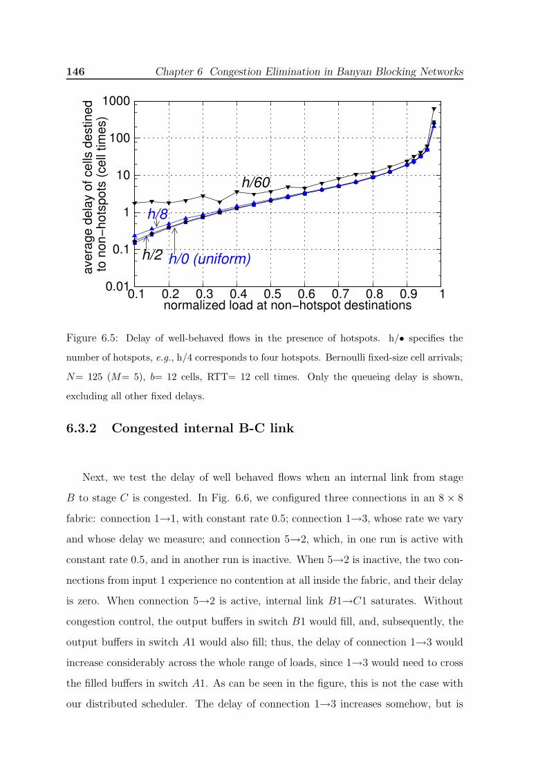
146 Chapter 6 Congestion Elimination in Banyan Blocking Networks
h/60
h/2 h/0 (uniform)
h/8
0.1 0.2 0.3 0.4 0.5 0.6 0.7 0.8 0.9 1normalized load at non−hotspot destinations
0.01
0.1
1
10
100
1000to
non
−hot
spot
s (c
ell t
imes
)av
erag
e de
lay
of c
ells
des
tined
Figure 6.5: Delay of well-behaved flows in the presence of hotspots. h/• specifies the
number of hotspots, e.g., h/4 corresponds to four hotspots. Bernoulli fixed-size cell arrivals;
N= 125 (M= 5), b= 12 cells, RTT= 12 cell times. Only the queueing delay is shown,
excluding all other fixed delays.
6.3.2 Congested internal B-C link
Next, we test the delay of well behaved flows when an internal link from stage
B to stage C is congested. In Fig. 6.6, we configured three connections in an 8 × 8
fabric: connection 1→1, with constant rate 0.5; connection 1→3, whose rate we vary
and whose delay we measure; and connection 5→2, which, in one run is active with
constant rate 0.5, and in another run is inactive. When 5→2 is inactive, the two con-
nections from input 1 experience no contention at all inside the fabric, and their delay
is zero. When connection 5→2 is active, internal link B1→C1 saturates. Without
congestion control, the output buffers in switch B1 would fill, and, subsequently, the
output buffers in switch A1 would also fill; thus, the delay of connection 1→3 would
increase considerably across the whole range of loads, since 1→3 would need to cross
the filled buffers in switch A1. As can be seen in the figure, this is not the case with
our distributed scheduler. The delay of connection 1→3 increases somehow, but is

6.3 Performance simulation results 147
A1
A2
A3
A4 B4
B3
B2
B1 C1
C2
C3
C4 8
7
6
5
4
3
11
2
3
4
5
6
7
8
load 0.5
load 0.5 bottleneck when 5−1 active
2??
(NO contention inside the fabric)connection 5 to 1 inactive
connection 5 to 1 active(link B1−C1 congested)
0 0.1 0.2 0.3 0.4 0.5normalized load of connection 1 to 3
0
5
10
15
20
aver
age
dela
y of
conn
ectio
n 1
to 3
(cel
l tim
es)
Figure 6.6: Delay of flow 1→3 when flow 5→2 is active (link B1-C1 saturated), and when
it is not (no internal link saturated). Bernoulli fixed-size cell arrivals; 8-port fabric, b=
12 cells, RTT= 12 cell times. Only the queueing delay is shown, excluding all other fixed
delays.
kept at moderate levels. Connection 1→3 experiences marginal delays at the ingress
linecard, due to contention with the backlogged cells from flow 1→17, and marginal
delays at switch A1.
6.3.3 Congested internal A-B link
Finally, we test the delay of well-behaved flows when an internal link from stage
A to stage B saturates. In Fig. 6.7, we configured connection 1→1, with constant
rate 0.5, connection 5→1, with varying rate, and connection 2→3, which, in one run
has rate 0.5, and in another run is inactive. When connection 2→3 is active, link
A1→B1 saturates. Connection 5→1, whose delay we measure, does not use neither
the bottleneck link, A1→B1, nor an upstream link. But it shares a crosspoint buffer in
switch C1 with the bottlenecked connection 1→1. If connection 1→1 delays to return
the credits for this buffer because it is bottlenecked at link A1→B1, the performance
of connection 5→1 might suffer (see section 6.2.1). As the figure demonstrates, when
the bottleneck is present, the delay of 5→1 fluctuates above the respective delay
when there is no bottleneck; however the delay discrepancy is only a few cell times.
7When the load of 1→3 equals 0.48, input 1 injects traffic at rate 0.98

148 Chapter 6 Congestion Elimination in Banyan Blocking Networks
A1
A2
A3
A4 B4
B3
B2
B1 C1
C2
C3
C4
1
2
3
4
5
6
7
8
load 0.5
bottleneck when 2−3 active
??
8
7
6
5
4
3
2
1load 0.5
2 to 3 inactive
2 to 3 active
(NO internal congestion)
(link A1−B1 congested)
20
10
1
0.1
0.01
aver
age
dela
y of
normalized load of connection 5 to 1 0 0.1 0.2 0.3 0.5 0.4
conn
ectio
n 5
to 1
(cel
l tim
es)
Figure 6.7: Delay of flow 5→1 when flow 1→3 is active (link A1-B1 saturated), and when
it is not (no internal contention). Bernoulli fixed-size cell arrivals; 8-port fabric, b= 12 cells,
RTT= 12 cell times. Only the queueing delay is shown, excluding all other fixed delays.
In another experiment, we used a request rate per link higher than one request per
cell time, and we observed that the delay of connection 5→1 increased considerably
at high input loads; actually, the system saturated at a rate of 0.46 for connection
5→1; this happens due to inefficient request throttling..

Chapter 7
Buffered Crossbars with Small
Crosspoint Buffers
7.1 Introduction
This chapter applies request-grant scheduling to single-stage buffered crossbars
so as to reduce their buffer size requirements. Traditional buffered cross-
bars operate under a credit-based type of flow control between the linecards and the
crosspoints buffers, and require one round-trip time (between the linecards and the
crossbar) worth of buffer space per crosspoint. This space is needed so that input
scheduler i (inside ingress linecard i) is able to continue writing new cells into cross-
point buffer i→ j, until it gets informed that output scheduler j (inside the crossbar)
reads these cells out of that buffer. In reality, if input i is the only one requesting
output j, the length of crosspoint buffer i→j will never grow beyond one (1) cell!
In this chapter, we position the per-input and per-output schedulers inside a central
scheduling chip; this placement allows us to speed up input-output coordination, thus
reducing the size of the flow control window down to one or two cells.
The credit prediction scheme that we proposed in section 3.3 essentially achieves
the same goal in switches with small, shared output queues: output queue size is made
independent of the cells-in-flight between the linecards and the fabric. However, in
that architecture, an output queue may accept concurrent arrivals, a drawback that
149
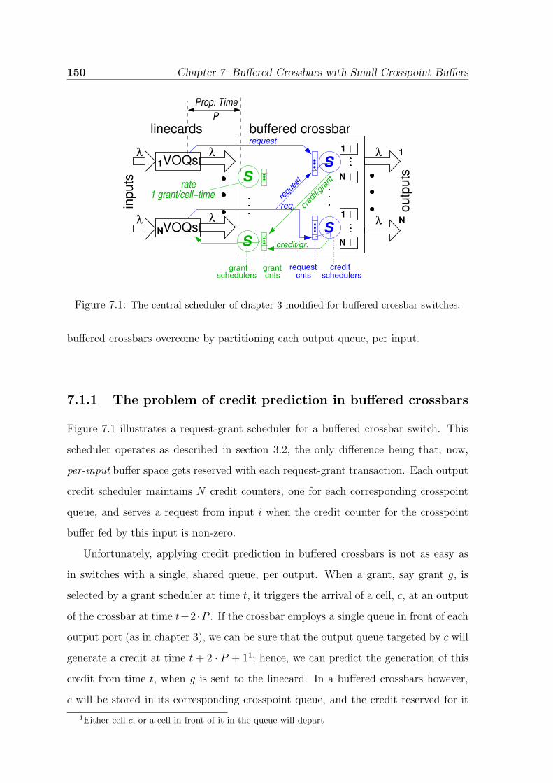
150 Chapter 7 Buffered Crossbars with Small Crosspoint Buffers
S
S
1
N
SN
1
Nλ
λ λ 1λ
λ
VOQs
VOQs
req.
credit/gr.
cred
it/gran
t
request
grant grantcnts
requestcnts
creditschedulersschedulers
Prop. Time
1 grant/cell−timerate
inpu
ts
outp
uts
linecardsP
λ1
N
S
buffered crossbar
reque
st
Figure 7.1: The central scheduler of chapter 3 modified for buffered crossbar switches.
buffered crossbars overcome by partitioning each output queue, per input.
7.1.1 The problem of credit prediction in buffered crossbars
Figure 7.1 illustrates a request-grant scheduler for a buffered crossbar switch. This
scheduler operates as described in section 3.2, the only difference being that, now,
per-input buffer space gets reserved with each request-grant transaction. Each output
credit scheduler maintains N credit counters, one for each corresponding crosspoint
queue, and serves a request from input i when the credit counter for the crosspoint
buffer fed by this input is non-zero.
Unfortunately, applying credit prediction in buffered crossbars is not as easy as
in switches with a single, shared queue, per output. When a grant, say grant g, is
selected by a grant scheduler at time t, it triggers the arrival of a cell, c, at an output
of the crossbar at time t+2 ·P . If the crossbar employs a single queue in front of each
output port (as in chapter 3), we can be sure that the output queue targeted by c will
generate a credit at time t + 2 · P + 11; hence, we can predict the generation of this
credit from time t, when g is sent to the linecard. In a buffered crossbars however,
c will be stored in its corresponding crosspoint queue, and the credit reserved for it
1Either cell c, or a cell in front of it in the queue will depart

7.2 A central scheduler for buffered crossbars 151
will be released only when the output scheduler decides to serve that crosspoint. At
time t, we do not know when this service will take place.
However, since we know all input grant schedulers that have sent grants for this
output, we can tell which crosspoint buffers will be non-empty when c arrives at
the crossbar; thus, with some extra logic, we can predict the decisions of the output
scheduler, and foretell when c is to release the buffer space reserved for it. The idea is
to make all scheduling decisions 2 ·P earlier than when a traditional scheduler would
make them. Assuming that the linecards react with a predictable delay to grants sent
to them, whatever the scheduler decides at time t determines the cells that will enter
the crossbar at time t + 2 · P , hence the crossbar traffic that will be switched at that
time.
7.2 A central scheduler for buffered crossbars
In this section, we present a new request-grant central scheduler for buffered cross-
bar switches, and we use this scheduler to implement credit prediction2. In buffered
crossbars, contrary to switches with shared output queues, there is no need for inputs
to request buffer space from per-output credit schedulers; instead, since each cross-
point buffer is private to some input, buffer space reservations can be performed by
independent (N), per-input schedulers.
Traditional buffered crossbars distribute these input schedulers into the N ingress
linecards. Figure 7.2(a) depicts the architecture with distributed input schedulers
and traditional credit-based flow control. In the worst case, N credits destined to the
same linecard can be generated in a single cell time, when all output schedulers serve
crosspoint queues from the same row of the crossbar. Despite this worst case rate,
in order to ensure stable switch operation, it suffices to sent one credit per linecard,
per cell time –i.e. equal to the peak rate at which a linecard forwards cells to the
crossbar.
2We could incorporate credit prediction directly into the scheduler of Fig. 7.1; however, the
scheduler that we present in this section has the benefit of being simpler.

152 Chapter 7 Buffered Crossbars with Small Crosspoint Buffers
S
S
S
S
S
SVOQ
VOQ
VOQ VOQ
VOQ
VOQ
S S SS S S
crossbar chiplinecardscrossbar chiplinecards
outp3outp2 outp3outp2outp1 outp1(a) (b)
credits request
grant
Figure 7.2: A 3×3, buffered crossbar switch (a) with the input schedulers distributed inside
the N ingress linecards; (b) with all input schedulers inside the crossbar chip.
7.2.1 Input line schedulers inside the crossbar chip
An alternative architecture, shown in Fig. 7.2(b), is to put all input link sched-
ulers inside the crossbar chip [Chrysos03b]. In the new scheme, each ingress linecard
communicates with the crossbar by sending one request, and receiving one grant, per
cell time. This request-grant protocol requires twice the average control throughput
of a traditional buffered crossbar, which is one credit per linecard per cell time.
Every time a cell arrives at a VOQ, the linecard issues a request to the respective
input scheduler. Each input scheduler remembers the outstanding requests using N ,
per-flow request counters; it also remembers the occupancy of the crosspoint buffers
along its row using N , per-flow credit counters, initialized at B, the size of crosspoint
buffers in cells. Even though all input schedulers reside in the same chip, each of
them operates independently, serving one request per cell time. Flows with non-zero
request and credit counters are eligible for service. Upon serving a request, the input
scheduler decrements by one the served request counter and the respective credit
counter; in parallel, it sends a grant to its corresponding ingress linecard. When the
linecard receives the grant, it immediately forwards the HOL cell of the granted VOQ
to the crossbar. In the baseline scheme, without credit prediction, the credit counter
is incremented by one when the output link scheduler forwards a cell to the output.
The data round-trip time equals the minimum delay between consecutive reser-

7.2 A central scheduler for buffered crossbars 153
vations of the same credit –i.e. one propagation delay, P , until the grant reaches the
linecard, plus another P delay until the injected cell reaches the crossbar, plus the
delay of the output link scheduling operation that releases the credit, plus the delay
of the input scheduling operation that reuses the released credit. Observe that this
round-trip time is similar as in traditional buffered crossbars.
7.2.2 Centralized scheduling in buffered crossbars: is it worth
trying?
Probably the most significant drawback of a request-grant scheduler for buffered cross-
bars is that it increases the minimum cell latency by two P delays. Apart from this
problem, the request-grant architecture has several benefits, stemming from its cen-
tralized character. The most attractive one, i.e. the capability to employ credit
prediction, is described in the next subsection. In the following paragraphs we dis-
cuss some additional implications of the centralized system.
For one, when a crosspoint buffer is served, a credit immediately returns to the
corresponding input scheduler, since credits do not cross chip boundaries; by contrast,
the distributed input schedulers of Fig. 7.2(a) receive credits with one P delay.
Moreover, up to N credits, one from each corresponding crosspoint, can readily reach
an input scheduler per cell time3. In the distributed architecture, an equivalent
operation would require a peak rate of N credits to be conveyed per linecard per cell
time, that is N/2 times more control bandwidth than that required by the request-
grant system. On the negative side, cell arrivals are imparted to the input schedulers
of the centralized architecture with one P delay. Also the input link schedulers add
to the complexity of the buffered crossbar chip4.
Several scheduling methods that try to maximize the throughput of buffered cross-
3Reference [Gramsamer02] shows that, under congestion epochs, performance improves when the
credits rate is unconstrained.4Observe that the distributed architecture may also use per-input schedulers inside the crossbar,
in order to serialize the credits that must be sent to the ingress linecards [Katevenis04]; the request-
grant architecture does not send credits, thus does not need these schedulers.

154 Chapter 7 Buffered Crossbars with Small Crosspoint Buffers
bars switches with small crosspoint buffers assume that each input and/or output
link scheduler has access to global switch information [Mhandi03] [Giaccone05]. By
maintaining global switch state in a central chip, the request-grant architecture fa-
cilitates the implementation of such systems: for instance, each individual per-input
or per-output link scheduler can examine the N 2 request counters –which mirror the
occupancy of the N 2 VOQs–, or the N 2 crosspoint buffers. A parameter often ne-
glected in the corresponding studies is that crosspoint buffers must anyhow be sized
proportionally to the round-trip time between the linecards and the crossbar. In
the next subsection, we present credit prediction, which radically lowers crosspoint
buffer requirements, by removing the round-trip time dependence; besides its inherent
significance, credit prediction also forms an excellent complement to methods that
achieve high throughput under small crosspoint buffers.
7.2.3 Credit prediction
To reduce the flow control window size, we predict the departures of cells from cross-
point queues two propagation times before they actually occur; thus, an input sched-
uler can reuse a credit, without having to wait until the respective cell reaches the
crossbar. To achieve this prediction, we incorporate N 2 virtual crosspoint counters,
and N virtual output schedulers, which are placed close to the input schedulers, inside
the crossbar chip (see Fig. 7.3). Each virtual output scheduler operates at the same
rate (one new selection per cell time), and implements the same selection discipline,
with its corresponding output link scheduler.
The prediction mechanism operates as follows. Consider a grant, gi→j, selected
by the grant scheduler for input i, at time5 t. At this time, gi→j is sent to ingress
linecard i, to trigger the injection of cell c into the crossbar; in parallel, virtual
crosspoint counter i→j is incremented by one, anticipating the enqueue operation of
cell c at crosspoint i→j, which will occur after a 2 · P delay, in the future, at time
t+2 ·P . At time t+1, the virtual output scheduler j selects one among the non-zero
5We measure time in cell times.

7.2 A central scheduler for buffered crossbars 155
S S S
S
S
S
VO
Q
linec
ards
inp3
inp2
inp1
request
schedulers
counters
counters
outp3outp2outp1
input virtual xpoint
virtual outputschedulers
grant
request
Figure 7.3: The schedulers needed for credit prediction in buffered crossbars; the input
schedulers reserve crosspoint buffer credits as in Fig. 7.2(b); the virtual output schedulers
“predict” the release of credits.
virtual crosspoint counters k→j, k ∈ [1, N ]; the selected crosspoint will actually send
a cell to its output after a 2 · P delay, i.e., at time t + 2 · P + 1. Upon this selection,
i.e., at time t + 1, the virtual scheduler decrements the selected virtual counter by
one, and increments the corresponding credit counter by one. Thus, if the selected
crosspoint counter corresponds to flow i→j, the credit reserved for grant gi→j will be
available to input scheduler i in time t + 2.
To see why this is feasible, consider the following two condition: (condition 1) the
non-zero virtual crosspoint counters for output j at time t correspond to the only
non-empty crosspoint queues for output j at time t +2 ·P ; (condition 2) the internal
state of the virtual output scheduler at time t is the same as that of the output
scheduler at time t + 2 · P . If conditions 1 and 2 are adhered to, then, the crosspoint
x that the virtual output scheduler serves at time t+1 (null if it serves none) is the
same as the crosspoint y that its corresponding output link scheduler serves at time
t+2·P+1.
Initially, all virtual credit counters are null, and all crosspoint queues are empty;
from that point on, if a virtual crosspoint counter is incremented by one, a cell will
definitely be enqueued in the respective crosspoint queue after 2 · P time; it follows
that condition 1 holds at start time. The virtual output scheduler starts with the
same state as its corresponding output link scheduler, thus, condition 2 also holds

156 Chapter 7 Buffered Crossbars with Small Crosspoint Buffers
at start time. If the virtual output scheduler and the link scheduler serve the same
crosspoint at time k and at time k+2·P , respectively, the two conditions will continue
to hold (for times k + 1 and k + 2 · P + 1); consequently, conditions 1 and 2 hold
continously, thus, the two schedulers visit the same crosspoints with a time lag of
2 · P .
Returing to our example, if the link scheduler for output j reads cell c at time
t + 2 · P + ν, ν ∈ N+, then, the virtual output scheduler j will have predicted that
future event already from time t+ν. Hence, at time t+ν +1, we can safely increment
by one the credit counter for crosspoint i→j, and reuse the space reserved for cell c
to generate a new i→j grant: at time t + 2 · P + ν + 1, when the cell utilizing this
new grant arrives at crosspoint queue i→j, cell c will have just departed from that
queue.
7.2.4 Data RTT using credit prediction
Using credit prediction, the effective data round-trip time equals the delay of a request
going through input and (virtual) output scheduling. If we name by D the delay
incurred in each such scheduling operation, then the round-trip time is 2 · D (i.e.
equal to SD according to the terminology of chapter 3). Thus, assuming that D=
1 cell time, the system will operate robustly with just two (2) cells buffer space
per crosspoint; even 1-cell buffer per crosspoint suffices when D≤ 1/2 cell times.
The buffer space needed is independent from the propagation delay (P ) between the
linecards and the crossbar. To the best of our knowledge, the only other scheme that
allows sizing the crosspoint buffers independent of the delay between the linecards
and the crossbar requires N -cell crosspoint buffers [Yoshigoe05].
Figure 7.4 depicts the timing of scheduling operations under credit prediction. The
figure assumes that (i) only connection 1→1 is active, (ii) each scheduling operation
incurs a delay, D, equal to one (1) cell time, (iii) B= 2 cells, and (iv) P= 2 cell
times. Without credit prediction, the buffer space per crosspoint required to sustain
full rate to connection 1→1 equals six (6) cells. In our example, we have two credits
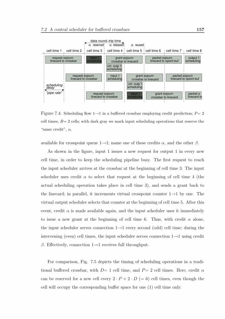
7.2 A central scheduler for buffered crossbars 157
cell time 6cell time 5cell time 4cell time 3cell time 2cell time 1 cell time 8
schedulingdelay"pipe rate"
cell time 7
reservedα reusedαreleasedαdata round−trip time
linecard to crossbarrequest sojourn
linecard to crossbarrequest sojourn grant sojourn
crossbar to linecard
linecard to xpoint bufpacket sojourngrant sojourn
crossbar to linecard
packet slinecard to
linecard to crossbarrequest sojourn grant sojourn
crossbar to linecardpacket sojourn
linecard to xpoint buf schedulingoutput 1
schedulinginput 1
schedulinginput 1
input 1
scheduling
scheduling
scheduling
virt. outp 1
virt. outp 1
Figure 7.4: Scheduling flow 1→1 in a buffered crossbar employing credit prediction; P= 2
cell times, B= 2 cells; with dark gray we mark input scheduling operations that reserve the
“same credit”, α.
available for crosspoint queue 1→1; name one of these credits α, and the other β.
As shown in the figure, input 1 issues a new request for output 1 in every new
cell time, in order to keep the scheduling pipeline busy. The first request to reach
the input scheduler arrives at the crossbar at the beginning of cell time 3. The input
scheduler uses credit α to select that request at the beginning of cell time 4 (the
actual scheduling operation takes place in cell time 3), and sends a grant back to
the linecard; in parallel, it increments virtual crosspoint counter 1→1 by one. The
virtual output scheduler selects that counter at the beginning of cell time 5. After this
event, credit α is made available again, and the input scheduler uses it immediately
to issue a new grant at the beginning of cell time 6. Thus, with credit α alone,
the input scheduler serves connection 1→1 every second (odd) cell time; during the
intervening (even) cell times, the input scheduler serves connection 1→1 using credit
β. Effectively, connection 1→1 receives full throughput.
For comparison, Fig. 7.5 depicts the timing of scheduling operations in a tradi-
tional buffered crossbar, with D= 1 cell time, and P= 2 cell times. Here, credit α
can be reserved for a new cell every 2 · P + 2 · D (= 6) cell times, even though the
cell will occupy the corresponding buffer space for one (1) cell time only.

158 Chapter 7 Buffered Crossbars with Small Crosspoint Buffers
cell time 7cell time 6cell time 5cell time 4cell time 3cell time 2cell time 1
data round−trip timereserved released reusedα α α
"pipe rate"
schedulingdelay
credit sojourncrossbar to linecardlinecard to crossbar
packet sojourn
credit sojourncrossbar to linecard
packet sojournlinecard to crossbar
input 1scheduling scheduling
output 1
schedulingoutput 1
input 1scheduling
schedulinginput 1
Figure 7.5: Scheduling flow 1→1 in a traditional buffered crossbar; P= 2 cell times, B= 2
cells; with dark gray we mark input scheduling operations that reserve the “same credit”,
α.
Figure 7.9 (page 165) illustrates the timing of scheduling operations when output
1 is requested by inputs 1 and 2, at the same time. Observe that the virtual scheduler
for output 1 always serves the same input (crosspoint) that output 1 will serve four
(4) cell times later. As can been seen, the occupancy of crosspoint buffers is always
≤ 2 cells.
7.2.5 Discussion
Since each output link scheduler always selects the same crosspoint that its corre-
sponding virtual output scheduler selected before 2 · P time, there is no reason to
recompute the same selection. Instead, the output lines of the crossbar can directly
implement the “program” computed by their corresponding virtual output scheduler.
For that purpose, we use one delay line per output, that stores and delays by 2 · P
the identifiers of the crosspoints selected by the virtual output schedulers.
Similarly, the N2 credit counters can be replaced by the virtual crosspoint coun-
ters. Input i will serve flow i→j, only if the virtual crosspoint counter i→j is ≤ B.
Another possibility is to place the per-input schedulers together with the per-
output virtual schedulers inside a separate scheduling chip, effectively removing com-
plexity from the buffered crossbar chip. This chip accepts requests and issues grants,
like the schedulers for bufferless fabrics. If we remove the output line schedulers from

7.2 A central scheduler for buffered crossbars 159
the crossbar chip, the scheduling chip will have to communicate the per-output cross-
point selections to the crossbar; otherwise, if we maintain the output line schedulers
inside the crossbar chip, no such communication will be needed.
Our description of credit prediction assumes that the HOL cells in crosspoint
queues can always be forwarded to the outputs. This may not hold however if these
cells are blocked due to backpressure exerted on the output ports of the crossbar.
Under these circumstances, credit prediction will not work properly, as credits may
not be generated at the time that the virtual output schedulers predict they will. In
section 3.3, we showed how to modify credit prediction so as to circumvent down-
stream backpressure. We can apply the same method here, by making virtual output
schedulers handle external backpressure signals: a virtual output scheduler serves a
virtual crosspoint counter only when it ensures that downstream backpressure will
not block the corresponding cell inside its crosspoint buffer.
7.2.6 Credit prediction when downstream backpressure is
present
Our description of credit prediction assumes that the HOL cells in crosspoint queues
can always be forwarded to the outputs. This may not hold however if these cells
are blocked due to backpressure exerted on the output ports of the crossbar. In this
section, we modify credit prediction to account for credit-based backpressure, exerted
upon fabric-output ports from nodes in the downstream direction. As in Section
3.3.1, we can work around this problem, if, instead of examining the downstream
backpressure state at the output ports of the fabric, i.e. for cells that have already
reached their crosspoint queue, we consult downstream backpressure before issuing
new grants. In this way we can ascertain that the cells that arrive into the crossbar
will always have downstream buffer space reserved, hence these will never need to
block in crosspoint queues.
Each virtual output scheduler maintains a downstream credit counter, used for
external backpressure purposes. Up to now, a virtual output scheduler could select a
virtual crosspoint counter (hence increment the credit counter for the corresponding

160 Chapter 7 Buffered Crossbars with Small Crosspoint Buffers
crosspoint) as long as this was non-zero. To account for external backpressure, we
require that the downstream credit counter also be non-zero. (The downstream credit
counter is decremented after serving a virtual crosspoint counter, and is incremented
when credits from the downstream node reach the virtual output scheduler6.) In this
way we guarantee that for every (predicted) credit that returns to the input scheduler,
there is buffer space reserved in the corresponding downstream buffer. Hence the cells
that use such (predicted) credits will have downstream buffer reserved when they
reach the crossbar, hence these will never need to block in crosspoint queues.
Now observe that there are no such downstream credits reserved for the cells that
the input schedulers can inject into the crossbar at start time: for each output, say
output j, the N input schedulers can generate a total of N × B grants using their
initial pool of credits, i.e. without consulting virtual output scheduler j first. The
cells that will use these grants will not have downstream buffer credits reserved when
they arrive at the crossbar. We can circumvent this problem, if the downstream
buffer has some extra space specificly allocated for these N × B cells7. Obviously,
the downstream credit counter, maintained by each virtual output scheduler, needs
to initialized at a value which is N × B smaller than the actual number of cells that
fit in the corresponding downstream buffer.
7.3 Performance simulation results
This section compares, by simulation, the performance of the centralized buffered
crossbar using credit prediction, to the performance of a traditional distributed buffered
crossbar. We use round-robin schedulers in both systems.
7.3.1 Delay performance
6Observe that this method increases the effective data round-trip time pertaining to the down-
stream (external) backpressure by the (internal) scheduler-linecard round-trip time.7Say that N= 64, that B= 2 cells, and that the cell size is 64 bytes; then, the extra buffer space
needed per downstream buffer is 64 Kbits, or 8 KBytes.

7.3 Performance simulation results 161
bernoulli
bursty12
buf. crossbar w. credit predictiontraditional buf. crossbartwo matching plots for:
and
0.1 0.2 0.3 0.4 0.5 0.6 0.7 0.8 0.9 1normalized input load
0.01
0.1
1
10
100
1000
aver
age
del
ay (c
ell t
imes
)
Figure 7.6: Performance for N= 32, P=0, D= 1/2 cell times, and B= 1 cell; Uniformly-
destined, Bernoulli and bursty (abs= 12 cells) cell arrivals; Only the queueing delay is
shown, excluding all fixed scheduling delays.
First, we compare the delay performance of the two systems under uniformly-
destined traffic. We assume a zero propagation delay (P= 0), and a delay per single-
resource scheduler, D, equal to 1/2 cell times; thus the flow control window in both
systems is 1 cell. Accordingly, we set the crosspoint buffer size, B= 1 cell. Figure
7.6 depicts mean queueing delay under Bernoulli cell arrivals, and under bursty cell
arrivals with average burst size (abs) equal to 12 cells. As can be seen, the two systems
perform identically.
7.3.2 Throughput for B=2 cells & increasing RTT
In this experiment, we set B= 2 cell times, and we measure switch throughput under
unbalanced Bernoulli cell arrivals, for varying round-trip times8: rtt= 1 (P= 0, D=
1/2), rtt= 2 (P= 0, D= 1), rtt= 12 (P= 5, D= 1), rtt= 32 (P= 15, D= 1), and rtt=
102 (P= 50, D= 1) As in [Rojas-Cessa01], w controls traffic unbalance (see Appendix
B).
8by rtt we denote the data round-trip time in the traditional buffered crossbar; with credit
prediction, the data round-trip time is equal to 2 ·D.

162 Chapter 7 Buffered Crossbars with Small Crosspoint Buffers
rtt 102
rtt 32
rtt 1rtt 2rtt 1
crosspoint buffer, B= 2 cells(NO credit prediction)
crosspoint buffer, B= 2 cells
four (4) matching plots for: rtt 12 rtt 102 rtt 2, ,rtt 32, and
rtt 12
(WITH credit prediction)
(a) (b)
0 0.1 0.2 0.3 0.4 0.5 0.6 0.7 0.8 0.9
norm
aliz
ed th
roug
hput
1.0
1 1 0.2 0.4 0.6 0.8 0unbalance factor, w
0.2 0.4 0.6 0.8 0unbalance factor, w
Figure 7.7: Throughput performance for varying rtt under unbalanced traffic; B= 2 cells;
full input load. (a) traditional buffered crossbar; (b) buffered crossbar employing credit
prediction.
Figure 7.7(a) depicts the performance of a traditional buffered crossbar. As can
be seen, performance is satisfactory only for rtt= 1 or 2 cell times; for larger rtt
values, performance declines. For rtt= 12 or 32 cell times, the system achieves full
throughput under uniformly-destined traffic (w= 0). Under uniform traffic, the load
at any particular output, j, comes evenly from all inputs, thus it utilizes all (32)
crosspoint buffers along the respective (j-th) column of the crossbar. This combined
buffer space equals 64 cells (32 × 2 cells), and can accommodate a rtt of 12 or 32
cell times. But with increasing w, the traffic for output j gradually concentrates
on input j, thus, it utilizes less buffer space; in the extreme case, when w= 1, the
2-cell crosspoint buffer j→j carries the total output load, thus rtt12, and rtt32,
yield normalized throughput 0.166, and 0.062, respectively, i.e. equal to 2/rtt. For
rtt= 102, the buffer space per output does not suffice to sustain switch throughput
for any w value: rtt102 yields a throughput of 2×32/102 (= 0.627), when traffic
is uniformly-destined (w= 0), and a throughput of 2/102 (= 0.019) when traffic is
completely unbalanced (w= 1).
Figure 7.7(b) depicts the performance of the buffered crossbar with credit pre-
diction. As can be seen, credit prediction yields high throughput for any round-trip
time, as the credit reserve and credit release operations occur contiguously inside the

7.3 Performance simulation results 163
rtt 32
rtt 102
rtt 12
rtt 102
rtt 32 rtt 12
rtt 2 rtt 2
crosspoint buffer size, "B = rtt"(NO credit prediction)
crosspoint buffer size, "B = rtt"(WITH credit prediction)
(b)(a)
0.2 0.4 0.6 0.8unbalance factor, w
1 0.2 0.4 0.6 0.8unbalance factor, w
1
1
0.9
0.8
0.7
0.6
norm
aliz
ed t
hrou
ghpu
t
0 0
Figure 7.8: Throughput performance for varying rtt under unbalanced traffic; in each plot,
B equals one rtt worth of traffic. (a) traditional buffered crossbar; (b) buffered crossbar
employing credit prediction.
crossbar chip.
7.3.3 Throughput for “B = RTT” and increasing RTT
In this experiment, everything is as in the previous section, but, in each particular
plot, we set the crosspoint buffer size, B, equal to one rtt worth of traffic. By doing
so, the system with no credit prediction operates robustly. As can be seen in Fig. 7.8,
for rtt= 2, both systems yield a normalized throughput around 0.88; with increasing
rtt, performance improves. In the traditional system, the buffer space per crosspoint
is always kept equal to the flow control window; in the system with credit prediction,
the buffer space increases above the effective flow control window, which is constant
and equal to 2 cells. Nevertheless, with increasing rtt, and thus with increasing B,
we witness similar throughput improvements in both systems, although with credit
prediction, the improvement is slightly higher.
We see that the performance of buffered crossbars under unbalanced traffic im-
proves with increasing crosspoint buffer size, even when, at the same time, the effective
data round-trip time increases proportionally. This implies that we do not need a
buffer of multiple flow control windows per crosspoint in order to improve the per-

164 Chapter 7 Buffered Crossbars with Small Crosspoint Buffers
formance of buffered crossbars (with or without credit prediction) under unbalanced
traffic: a single, large flow control window buffer suffices.

7.3
Perfo
rmance
simula
tion
results
165
cell time 5cell time 4cell time 3cell time 2 cell time 6cell time 1 cell time 9 cell time 10 cell time 11 cell time 12
crossbar to linecardgrant 1−1 sojourn
crossbar to linecardgrant 2−1 sojourn
crossbar to linecardgrant 1−1 sojourn
linecard to xpoint bufpacket 1−1 sojourn
linecard to xpoint bufpacket 2−1 sojourn
linecard to xpoint bufpacket 1−1 sojourn
linecard to xpoint bufpacket 2−1 sojourn
linecard to xpoint bufpacket 1−1 sojourn
linecard to xpoint bufpacket 2−1 sojourn
linecard to xpoint bufpacket 1−1 sojourn
crossbar to linecardgrant 2−1 sojourn
crossbar to linecardgrant 2−1 sojourn
crossbar to linecardgrant 1−1 sojourn
crossbar to linecardgrant 1−1 sojourn
schedulinginput 1
schedulinginput 1
xpoint 1−1: 0xpoint 2−1: 0
xpoint 1−1: 0xpoint 2−1: 0
xpoint 1−1: 0xpoint 2−1: 0
xpoint 1−1: 0xpoint 2−1: 0
xpoint 1−1: 0xpoint 2−1: 0
xpoint 1−1: 1xpoint 2−1: 1
xpoint 1−1: 1xpoint 2−1: 2
xpoint 1−1: 2xpoint 2−1: 1
xpoint 1−1: 1xpoint 2−1: 2
xpoint 1−1: 2xpoint 2−1: 1
input 2scheduling
schedulinginput 2
schedulinginput 1
schedulinginput 2
scheduling
output 1serves in1
output 1serves in2
serves in2output 1
serves in1output 1
serves in1output 1input 1
serves in1
serves in2
serves in1
serves in2
serves in1
virt. outp 1
virt. outp 1
virt. outp 1
virt. outp 1
virt. outp 1
Figu
re7.9:
Sch
edulin
gflow
s1→
1an
d2→
1in
abuffered
crossbar
employ
ing
credit
pred
ic-
tion;w
eassu
me
that
both
request
counters
1→1
and
2→1
arenon
-zerofrom
the
begin
nin
g
ofcell
time
1;P
=2
celltim
es,B
=2
cells.

166 Chapter 7 Buffered Crossbars with Small Crosspoint Buffers

Chapter 8
Conclusions
This dissertation has studied multistage switching fabrics, exploring ways to-
wards scalable, low cost, and robust switching systems. In this effort, conges-
tion management has been identified as a central, open issue: to deal with it using
prior state-of-the-art, one could either employ a bufferless fabric with a costly control
unit and poor performance, or a buffered fabric with a large number of queues, as re-
quired in order to segregate flows heading to different fabric-outputs. Unfortunately,
none of these solutions scales well.
8.1 Contributions
8.1.1 Request-grant scheduled backpressure
We have proposed and evaluated request-grant backpressure, a realistic scheduling
architecture for multistage buffered switching fabrics. The new architecture relies on
independent, single-resource schedulers, operating in a pipeline. It unifies the ideas
of central scheduling for bufferless fabrics and of distributed scheduling for buffered
fabrics, it provides very good performance at realistic cost, and it demonstrates the
latency - buffer space tradeoff: it avoids the many buffers that are normally required in
order to avoid HOL blocking by delaying packets by the time needed for coordination.
The request-grant scheduled backpressure protocol economizes on buffer space
relative to per-flow buffer reservation and backpressure. Effectively, instead of first
167

168 Chapter 8 Conclusions
letting data occupy buffers and then scheduling among the flows to which these data
belong (“corrective” congestion management), we schedule first among competing
requests and then let into the fabric only those data that are known to be able to
quickly get out of it (“preventive” congestion management). Despite their differences,
request-grant scheduled backpressure compares to per-flow queueing in that both
schemes explicitly disallow congestion expansion; the contribution of the new scheme
is that it requires considerably less buffer space than per-flow queueing.
Request-grant scheduled backpressure is very different, and in certain aspects
much more efficient than reactive congestion management. Reactive congestion man-
agement allows packets to reach close to the congestion point but then tries to secure
extra buffer space that still remains unoccupied, or it allows congestion to develop
and subsequently tries to break it. The main drawback is that once you allow too
many packets into the network (like too many cars into a highway intersection) but
lack the capacity to store them into per-destination queues, congestion can develop,
thus hurting the performance of well-behaved flows. Under reactive congestion man-
agement, even if the sources (end or local) contributing to congestion are eventually
throttled, transient inefficiencies cannot easily be avoided, while flows may be slowed
down harshly, beyond what is actually necessary. In principle, it takes time to dis-
tinguish short-term from long-term contention (congestion) in a distributed setup.
Commonly, queue occupancy thresholds are used to detect congestion. A proper oc-
cupancy threshold value may depend on packet size distribution, flow control round-
trip time, burst size, multiplexing degree, and many other parameters. Too low a
threshold may bring false-positives with all their consequences (wasting resources,
needlessly throttling sources, etc.); on the other hand, too high a threshold will allow
queues to grow before actions apply, thus deteriorating performance.
By contrast, in our proposal, the congestion avoidance protocol is embedded in the
normal switch operation, making the detection of congestion epochs transparent; in
addition, the scheme works robustly independent of the number of congestion points.
In our view, these features render request-grant scheduled backpressure very effective
under heavy traffic; under moderate traffic, it is advantageous to employ a reactive

8.1 Contributions 169
scheme that will not penalize lightly loaded flows with the request-grant, cold-start
latency.
Request-grant backpressure uses a scheduling network to filter the excessive de-
mands out. Effectively, the data allowed inside the fabric that are destined to a given
link never exceed the buffer capacity in front of that link. In this way we avoid HOL
blocking, since packets are very rarely slowed down at the head of a queue due to
downstream backpressure. This allows us to build shared queues inside the data net-
work, without worrying about flow interference: the data network needs only perform
the switching function, and resolve occasional (short-term) packet conflicts: it does
not have to deal with congestion. Even though congestion is eliminated in the data
network, the scheduling network is loaded with uncoordinated requests, thus being
itself subject to congestion. We circumvent request congestion via per-flow request
queues. Implementing per-flow queues in the scheduling network requires significantly
less memory bandwidth and significantly fewer memory bits than in the payload data
network; this is so because the scheduling network operates on packet headers rather
than packet payload. In addition, the per-flow request queues can be implemented
using per-flow counters, radically reducing cost. By isolating the requests from dif-
ferent flows, the scheduling network can allocate fair and efficient shares (even using
flow weights), while the fabric, by acting transparently (i.e., not developing HOL
blocking), is guaranteed to accept these scheduled rates.
8.1.2 Centralized vs. distributed arbitration
The single-resource schedulers that comprise the scheduling network can either be dis-
tributed through the fabric or can be placed all inside a central chip. The centralized
solution enables faster access to global information, improving coordination and per-
formance. These benefits are exploited in threshold grant throttling (section 3.5.3),
so that outputs can identify bottleneck inputs and stop issuing grants to them, and
in credit prediction (sections 3.3 and 7.2.3), so that inputs can reuse buffer space,
being immediately informed when outputs are going to match with them, without
having to wait for a long, off-chip feedback delay. Although there are similarities, the

170 Chapter 8 Conclusions
centralized control that we propose is quite different from the one used in bufferless
VOQ switches. On the one hand, both control systems maintain central state for N 2
flows, which certainly limits their scalability. On the other hand, our control com-
prises single-resource schedulers that are independent from each other and operate in
a pipeline. This helps to distribute state and functions over multiple (central) control
chips. By contrast, the scheduling algorithms proposed for bufferless fabrics comprise
single-resource schedulers that are dependent; furthermore, they need multiple iter-
ations of handshaking in order to improve matching quality. Such closely coupled
schedulers cannot be easily put apart.
8.1.3 Applications
We have applied request-grant scheduled backpressure in several settings:
- Shared-memory switches with small output queues: The request-grant sched-
uler that we proposed for shared-memory switches (chapter 3) generalizes the
centralized arbiters used in bufferless crossbars, demonstrating some very inter-
esting properties. The availability of small buffer space at the output ports can
decouple the scheduling operations at input ports from the scheduling opera-
tions at output ports, thus enabling pipelined operation, as in buffered cross-
bars. At the same time, with 12-cell buffer space per output1, performance is
higher than that of buffered crossbars, which use an aggregate buffer space of
N cells per output. However, as the output buffer space is small (<< N cells),
and is shared among N inputs, we need to control buffer usage. This bears
analogies with the desynchronization needed in bufferless crossbars. However,
thanks to the few buffers in the shared-memory system, we do not need deter-
ministic (full) desynchronization as in bufferless crossbars, but just statistical
desynchronization, which will prevent severe (nearly full) synchronization.
- Non-blocking three-stage Clos/Benes fabrics: In this setting, which constitutes
the core of this dissertation, we used request-grant backpressure in multistage
1Independent of N , and independent of the distance between the linecards and the fabric.

8.1 Contributions 171
fabrics, in order to prevent congested outputs from deteriorating the perfor-
mance of unrelated flows. We demonstrated the feasibility of a non-blocking,
ten Terabit/s system, with 1024 ports, made of ninety-six, single-chip, 32× 32
buffered crossbar switches in a three-stage Benes arrangement; the scheduling
subsystem that implements the request-grant scheduled backpressure is accom-
modated in a single, central control chip. The datapath of the fabric employs
inverse multiplexing (multipath routing) on a per packet basis, thus enabling
fully asynchronous switch operation. The request-grant scheduler also explic-
itly limits the extent of out-of-order packets resulting from multipath routing;
effectively, for a 1024-port fabric, a reorder buffer of size equal to a few tens of
kilobytes at each fabric-output can guarantee fully in-order delivery. Extensive
performance simulations indicate that our system can continue offering very
low delays to the packets heading to non-congested destinations, even when
nearly all other destinations are congested. To our knowledge, these findings
are among the few leading ones towards robust, non-blocking fabrics.
- Blocking three-stage banyan fabrics: Compared to non-blocking network topolo-
gies, like the Benes fabric, blocking topologies, such as the banyan network,
place additional constraints upon traffic schedules due to the limited capacity
of the internal network. Effectively, besides banyan-output ports, congestion
can develop at internal banyan links as well. We proposed a fully distributed
request-grant scheduler that manages both internal and output-port congestion
in three-stage, output-buffered, banyan networks.
- Buffered crossbars with no-RTT dependence: We devised a novel method (credit
prediction) that makes the crosspoint buffer space independent of the propa-
gation delay between the linecards and the crossbar, i.e. independent of the
number of cells in transit between these two units. This is a significant im-
provement over traditional buffered crossbars, which, as the distance between
the linecards and the fabric grows, and as the line rate increases, potentially
require an excessive amount of on-chip memory.

172 Chapter 8 Conclusions
8.2 Future work
There are several ways to improve and extend the work presented in this thesis. From
within a long list of open issues, we distinguish the following three.
8.2.1 Avoid request-grant latency under light traffic
The request-grant protocol imposes a cold-start latency. For lightly loaded flows,
it is desirable to avoid this extra delay in latency-sensitive applications, e.g. clus-
ter/multiprocessor interconnects. To achieve this, we need to send some few cells
in blind-mode (without requests and grants) in order to minimize their delay; but
when there are indications that the fabric may be heavily loaded, we need to return
to request-grant transactions; as proposed in section 2.3.2, one can employ a mech-
anism similar to RECN’s set-aside-queues (SAQs) [Duato05] so as to prevent “free”
cells from congesting the network. Under what circumstances will the system toggle
between the two types of operation, and which flows will each transition affect, are
among the problems that one has to solve in this effort. A framework for this study
has been proposed in section 2.2.2.
8.2.2 Different network topologies, different switch architec-
tures
In this thesis we considered Benes/Clos networks that provide non-blocking opera-
tion at the minimum possible cost; we also considered banyan networks as a good
representative of indirect blocking networks. Certainly, several other network topolo-
gies exist. A prominent network topology that is currently used in many commercial
products is the fat tree [Leiserson85]. The capacity of a fat tree can be tailored to
meet the application’s requirements: depending on the bandwidth provisioned for
internal links, fat trees can have zero or controlled amount of internal blocking. In
addition, fat trees are by convention bidirectional, thus they can route the control
packets that travel opposite to the direction of payload packets, e.g. credits, grants,
acknowledgments, etc., through the regular data links; in this way, fat trees remove

8.2 Future work 173
the cost of implementing separate physical links for control communication. For these
reasons, it is interesting to explore whether and at what cost request-grant scheduled
backpressure can be applied to fat tree networks.
An orthogonal issue is the architecture of the switching elements. In this thesis we
only considered fabrics made of buffered crossbar switches, but request-grant back-
pressure can operate on other switch architectures as well. One switch architecture
that is certainly worth studying is the combined input-output queueing (CIOQ).
8.2.3 Optimizing buffer-credits distribution
When using request-grant scheduled backpressure, credit accumulations (credit hog-
ging) constitute a problem analogous to buffer hogging in networks that use hop-by-
hop backpressure. Whereas buffer hogging occurs when outputs are congested, credit
hogging shows up under congested inputs. An encouraging fact is that inputs can
only be congested on a transient basis –not in the long run. In this thesis we came
up with the threshold grant throttling solution (section 3.5.3) to deal with transients
with congested inputs. Although this solution is very effective, it is best suited for
centralized architectures. Dealing with congested inputs in a distributed environment
requires further study.

174 Chapter 8 Conclusions

Bibliography
[Abel03] F. Abel, C. Minkenberg, R. Luijten, M. Gusat, I. Iliadis: “A Four-Terabit
Packet Switch Supporting Long Round-Trip Times”, IEEE Micro Magazine, vol.
23, no. 1, Jan-Feb 2003, pp. 10-24.
[Anderson94] T. Anderson, S. Owicki, J. Saxe, C. Thacker: “High-Speed Switch
Scheduling for Local-Area Networks”, ACM Transactions on Computer Systems,
vol. 11, no. 4, November 1993, pp. 319-352.
[Benes64] V. Benes: “Optimal Rearrangeable Multistage Connecting Networks”, Bell
Systems Technical Journal, vol. 43, no. 7, July 1964, pp. 1641-1656.
[Bianco05] A. Bianco, P. Giaccone, E. M. Giraudo, F. Neri, E. Schiattarella: “Perfor-
mance Analysis of Storage Area Network Switches”, Proc. IEEE HPSR, Hong-
Kong, May 2005.
[Chao03] J. Chao, Z. Jing, S.Y. Liew: “Matching Algorithms for Three-Stage Buffer-
less Clos Network Switches”, IEEE Communications Magazine, October 2003,
pp. 46-54.
[Chiussi97] F. M. Chiussi, J. G. Kneuer, V. P. Kumar: “The ATLANTA architecture
and chipset”, IEEE Communication Magazine, December 1997, pp. 44-53.
[Chiussi98] F. Chiussi, D. Khotimsky, S. Krishnan: “Generalized Inverse Multi-
plexing for Switched ATM Connections” Proc. IEEE GLOBECOM, Australia,
November 1998, pp. 3134-3140.
175
176 BIBLIOGRAPHY
[Chrysos02] N. Chrysos, M. Katevenis: “Transient Behavior of a Buffered Crossbar
Converging to Weighted Max-Min Fairness”, Inst. of Computer Science, FORTH,
August 2002, 13 pages; http://archvlsi.ics.forth.gr/bufxbar/
[Chrysos03a] N. Chrysos, M. Katevenis: “Weighted Fairness in Buffered Cross-
bar Scheduling”, Proc. IEEE HPSR, Torino, Italy, June 2003, pp. 17-22;
http://archvlsi.ics.forth.gr/bufxbar/
[Chrysos03b] N. Chrysos: “Design Issues of a Multiple-Priority, Variable-Size-
Packet Buffered Crossbar”, Inst. of Computer Science, FORTH, October 2003;
http://archvlsi.ics.forth.gr/bufxbar
[Chrysos04a] N. Chrysos, M. Katevenis: “Multiple Priorities in a Two-Lane Buffered
Crossbar”, Proc. IEEE GLOBECOM, TX, USA, Nov-Dec 2004, CR-ROM paper
ID ”GE15-3”.
[Chrysos04b] N. Chrysos, I. Iliadis, C. Minkenberg: “Architecture and Performance
of the Data Vortex Photonic Switch”, IBM Research Report, RZ3562, November
2004.
[Chrysos05] N. Chrysos, M. Katevenis: “Scheduling in Switches with Small Inter-
nal Buffers”, Proc. IEEE GLOBECOM, St. Louis, MO USA, Nov-Dec 2005;
http://archvlsi.ics.forth.gr/bpbenes
[Chrysos06] N. Chrysos, M. Katevenis: “Scheduling in Non-Blocking Buffered Three-
Stage Switching Fabrics”, Proc. IEEE INFOCOM, Barcelona, Spain, April 2006.
[Chrysos06b] N. Chrysos, M. Katevenis: “Preventing Buffer-Credit Accumulations
in Switches with Shared Small Output Queues”, Proc. IEEE HPSR, Poznan,
Poland, June 2006, pp. 409-416.
[Clos53] C. Clos: “A Study of Non-Blocking Switching Networks”, Bell Systems Tech-
nical Journal, vol. 32, no. 2, March 1953, pp. 406-424.

BIBLIOGRAPHY 177
[Demers89] A. Demers, S. Keshav, S. Shenker: “Design and Analysis of a Fair Queue-
ing Algorithm”, Proc. ACM SIGCOMM, Austin TX USA, September 1989, pp.
1-12.
[Duato04] J. Duato, J. Flich, T. Nachiondo: “A Cost-Effective Technique to Reduce
HOL Blocking in Single-Stage and Multistage Switch Fabrics”, Euromicro Con-
ference on Parallel, Distributed and Network-Based Processing, February 2004,
pp. 48-53.
[Duato05] J. Duato, I. Johnson, J. Flich, F. Naven, P. Garcia, T. Nachiondo: “A New
Scalable and Cost-Effective Congestion Management Strategy for Lossless Mul-
tistage Interconnection Networks”, Proc. 11th IEEE Symp. High-Performance
Computer Architecture (HPCA), San Francisco, CA USA, February 2005, pp.
108-119.
[Garcia05] P.J. Garcia, J. Flich, J. Duato, I. Johnson, F.J. Quiles, F. Naven: “Dy-
namic Evolution of Congestion Trees: Analysis and Impact on Switch Archi-
tecture”, Lecture Notes in Computer Science (HIPEAC), November 2005, pp.
266-285.
[Georgakopoulos04a] G. Georgakopoulos: “Nash Equilibria as a Fundamental Issue
Concerning Network-Switches Design”, Proc. IEEE ICC, Paris, France, June
2004, vol. 2, pp. 1080-1084.
[Georgakopoulos04b] G. Georgakopoulos: “Few buffers suffice: Explaining why and
how crossbars with weighted fair queuing converge to weighted max-min fair-
ness”, Dept. of Computer Science, Technical Report, Greece, July 2003, 6 pages;
http://archvlsi.ics.forth.gr/bufxbar/
[Giaccone05] P. Giaccone, E. Leonardi, D. Shah: “On the Maximal Throughput of
Networks with Finite Buffers and its Application to Buffered Crossbars”, Proc.
IEEE INFOCOM, Miami USA, vol. 2, March 2005, pp. 971-980.

178 BIBLIOGRAPHY
[Gianatti94] S. Gianatti, A. Pattavina: “Performance Analysis of ATM Banyan Net-
works with Shared Queueing –Part I: Random Offered Traffic”, IEEE Transac-
tions on Communications, vol. 2, no. 4, August 1994, pp. 398-410.
[Goke73] L. R. Goke, G. J. Lipovski: “Banyan networks for partitioning multipro-
cessor systems”, in Proc. First IEEE Symp. Computer Architecture, December
1973, pp. 21-28.
[Gramsamer02] F. Gramsamer, M. Gusat, R. P. Luijten: “Optimizing Flow Control
for Buffered Switches”, Proc. 11th Conference on Computer Communications
and Networks, October 2002, pp. 438-443.
[Gusat05] M. Gusat, D. Craddock, W. Denzel, T. Engbersen, N. Ni, G. Pfister, W.
Rooney, J. Duato: “Congestion Control in InfiniBand Networks”, HOT ICTS 13,
A Symp. on High Performance Interconnects, August 2005, Stanford University,
California.
[Hahne91] E. Hahne: “Round-Robin Scheduling for Max-Min Fairness in Data Net-
works”, IEEE Journal on Selected Areas in Communications (JSAC), vol. 9, no.
7, September 1991, pp. 1204-1039.
[Hahne98] A. K. Choudhury, E. Hahne: “Dynamic Queue Length Thresholds for
Shared-Memory Packet Switches”, IEEE/ACM Transactions on Networking, vol.
6, no. 2, April 1998, pp. 130-140.
[Han03] M.S. Han, D.Y. Kwak, B. Kim: “Desynchronized Input Buffered Switch
with Buffered Crossbar”, IEICE Transactions Communications vol. E86-B, no.
7, July 2003, pp. 2216-2219.
[Iliadis95] I. Iliadis: ”A new feedback congestion control policy for long propagation
delays”, IEEE Journal on Selected Areas in Communications (JSAC), vol. 13,
September 1995, pp. 1284-1294.
[Iliadis04] I. Iliadis, N. Chrysos, C. Minkenberg: “Performance Evaluations of the
Data Vortex Photonic Switch”, IBM Research Report, RZ3603, April 2005.

BIBLIOGRAPHY 179
[InfiniBand] InfiniBandTM , Trade Association, http://www.infiniband.com
[Iyer03] S. Iyer, N. McKeown: “Analysis of the parallel packet switch architecture”,
IEEE/ACM Transactions on Networking, 2003, pp. 314-324.
[Iyer05] S. Iyer, S. Chuang, N. McKeown: “Practical algorithms for performance
guarantees in buffered crossbars”, Proc. IEEE INFOCOM, Miami, USA, March
2005.
[Javidi01] T. Javidi, R. Magill, T. Hrabik: ”A High-Throughput Scheduling Algo-
rithm for a Buffered Crossbar Switch Fabric” Proc. IEEE ICC, vol. 5, Helsinki,
Finland, June 2001, pp. 1586-1591.
[Kabacinski03] W. Kabacinski, C-T. Lea, G. Xue - Guest Editors: 50th Anniversary
of Clos networks –a collection of 5 papers, IEEE Communications Magazine, vol.
41, no. 10, October 2003, pp. 26-63.
[Karol87] M. J. Karol, M. G. Hluchyj, S. P. Morgan: “Input Versus Output Queueing
on a Space-Division Packet Switch”, IEEE Transactions on Communications,
vol. COM35, no.12, December 1987, pp. 1347-1356.
[Katevenis87] M. Katevenis: “Fast switching and Fair Control of Congested Flow
in Broad-Band Networks”, IEEE Journal on Selected Areas in Communication
(JSAC), vol. 5, no. 8, October 1987, pp. 1315-1326.
[Katevenis95] M. Katevenis, P. Vatsolaki, A. Efthymiou: “Pipelined Memory Shared
Buffer for VLSI Switches”, Proc. ACM SIGCOMM, Cambridge, MA USA, Aug-
Sep. 1995, pp. 39-48.
[Katevenis98] M. Katevenis, D. Serpanos, E. Spyridakis: “Credit-Flow-Controlled
ATM for MP Interconnection: the ATLAS I Single-Chip ATM Switch”, Proc.
4th IEEE Symp. High-Performance Computer Architecture (HPCA), Las Vegas,
NV USA, February 1998, pp. 47-56; http://archvlsi.ics.forth.gr/atlasI/
[Katevenis04] M. Katevenis, G. Passas, D. Simos, I. Papaefstathiou, N.
Chrysos: “Variable Packet Size Buffered Crossbar (CICQ) Switches”,
180 BIBLIOGRAPHY
Proc. IEEE ICC, Paris, France, vol. 2, June 2004, pp. 1090-1096;
http://archvlsi.ics.forth.gr/bufxbar
[Katevenis05] M. Katevenis, G. Passas: “Variable-Size Multipacket Segments in
Buffered Crossbar (CICQ) Architectures”, Proc. IEEE ICC, Seoul, Korea, May
2005, paper ID ”09GC08-4”; http://archvlsi.ics.forth.gr/bufxbar/
[Khotimsky01] D. Khotimsky, S. Krishnan: “Stability analysis of a parallel packet
switch with bufferless input demultiplexors”, Proc. IEEE ICC, June 2001, pp.
100-111.
[Kleinrock80] M. Gerla, L. Kleinrock: “Flow Control: A comparative Survey”,
IEEE/ACM Transactions on Networking vol. COM-28, no. 4, April 1980.
[Kornaros99] G. Kornaros, D. Pnevmatikatos, P. Vatsolaki, G. Kalokerinos, C. Xan-
thaki, D. Mavroidis, D. Serpanos, M. Katevenis: “ATLAS I: Implementing a
Single-Chip ATM Switch with Backpressure”, IEEE Micro, vol. 19, no. 1, Jan-
Feb 1999, pp. 30-41.
[Krishan99] P. Krishna, N. Patel, A. Charny, R. Simcoe: “On the Speedup Required
for Work-Conserving Crossbar Switches”, IEEE Journal Selected Areas in Com-
munications (JSAC), vol. 17, no. 6, June 1999, pp. 1057-1066.
[LaMaire94] R. LaMaire, D. Serpanos: “Two-Dimensional Round-Robin Schedulers
for Packet Switches with Multiple Input Queues”, IEEE/ACM Transactions on
Networking, vol. 2, no. 5, October 1994, pp. 471-482.
[Leiserson85] C. E. Leiserson: “Fat-trees: universal networks for hardware-efficient
supercomputing”, IEEE Transactions on Computers, vol. 34 , October 1985, pp.
892-901.
[Li92] S. Q. Li: “Performance of a Nonblocking Space-Division Packet Switch with
Correlated Input Traffic”, IEEE Transactions on Communications, vol. 40, no.
1, January 1992, pp. 97-107.
BIBLIOGRAPHY 181
[Lin04] M. Lin, N. McKeown: “The Throughput of a Buffered Crossbar Switch”,
IEEE Communication Letters, vol. 9, May 2005, pp. 465-467.
[Luijten01] R.P.Luijten, T.Engbersen, C.Minkenberg: “Shared Memory Switching +
Virtual Output Queuing: a Robust and Scalable Switch” Proc. IEEE ISCAS,
Sydney, Australia, May 2001, pp. IV-274-IV-277.
[Luijten03] R. Luijten, C. Minkenberg, M. Gusat: “Reducing memory size in buffered
crossbars with large internal flow control latency”, Proc. IEEE GLOBECOM,
vol. 7, December 2003, pp. 3683-3687.
[LCS] PMC-SIERRA: “Linecard to Switch (LCS) Protocol”, http://www.pmc-
sierra.com/pressRoom/pdf/lcs wp.pdf
[Magill03] B. Magill, C. Rohrs, R. Stevenson: “Output-Queued Switch Emulation by
Fabrics With Limited Memory”, IEEE Journal on Selected Areas in Communi-
cations (JSAC), May 2003, pp. 606-615.
[Marsan02] M. A. Marsan, A. Biano, P. Giaccone, E. Leonardi, F. Nero: “Packet-
Mode Scheduling in Input-Queued Cell-Based Switches”, IEEE Transactions on
Networking, vol. 10, no. 5, October 2002, pp. 666-678.
[McKeown95] N. McKeown: “Scheduling Algorithms for Input-Queued Cell
Switches”, Ph.D. Thesis, University of California at Berkeley, May 1995.
[McKeown99a] N. McKeown: “The iSLIP Scheduling Algorithm for Input-Queued
Switches”, IEEE/ACM Transactions on Networking, vol. 7, no. 2, April 1999,
pp. 188-201.
[McKeown99b] N. McKeown, A. Mekkittikul, V. Anantharam, J. Walrand: “Achiev-
ing 100% Throughput in an Input-Queued Switch”, IEEE Transactions on Com-
munications, vol. 47, no. 8, August 1999. pp. 1260-1267.
[Mhandi03] L. Mhamdi, M. Hamdi: “MCBF: A High-Performance Scheduling Algo-
rithm for Buffered Crossbar Switches”, IEEE Communications Letters, vol. 7,
no. 9, September 2003, pp. 451-453.

182 BIBLIOGRAPHY
[Mhamdi04] L. Mhamdi, M. Hamdi: “Scheduling Multicast Traffic in Internally
Buffered. Crossbar Switches”, Proc. IEEE ICC, Paris, France, vol. 2, June 2004,
pp. 1103-1107.
[Minkenberg00] C. Minkenberg, T. Engbersen: “A Combined Input and Output
Queued Packet-Switched System Based on A PRIZMA Switch-on-a-Chip Tech-
nology”. IEEE Communications Magazine, vol. 38, no. 12, December 2000, pp.
70-77.
[Minkenberg01] C. Minkenberg: “On Packet Switch Design”, Ph.D. Thesis, Technical
University Eindhoven, The Netherlands, September 2001.
[Minkenberg02] C. Minkenberg, R.P. Luijten, F. Abel, W. Denzel, M. Gusat: Current
Issues in Packet Switch Design”, Proc. HOTNETS, Princeton, USA, October
2002.
[Ni01] N. Ni, L. N. Bhuyan: “Fair Scheduling for Input Buffered Switches”, Parallel
and Distributed Processing Symposium (IPDPS’01) Workshops.
[Pappu03] P. Pappu, J. Parwatikar, J. Turner, K. Wong: “Distributed Queue-
ing in Scalable High Performance Routers”, Proc. IEEE INFOCOM, vol. 3,
April/March 2003, pp. 1633-1642.
[Pappu04] P. Pappu, J. Turner, K. Wong: “Work-Conserving Distributed Schedulers
for Terabit Routers”, Proc. ACM SIGCOMM, September 2004, pp. 257-268.
[Parekh93] A. K. Parekh, R. G. Gallager: “A Generalized Processor Sharing Ap-
proach to Flow Control in Integrated Services Networks: The single Node Case”,
IEEE/ACM Transactions on Networking, vol. 1, no. 3, June 1993, pp. 344-357.
[Passas03] G. Passas: “Performance Evaluation of Variable Packet Size Buffered
Crossbar Switches”, Technical Report FORTH-ICS/TR-328, Thesis, Univ. of
Crete, November 2003, 46 pages.

BIBLIOGRAPHY 183
[Peh00] L. Peh, W. Dally: “Flit-Reservation Flow Control”, Proc. of the 6th Sympo-
sium on High Performance Computer Architecture (HPCA), Toulouse, France,
January 2000, pp. 73-84.
[Pfisher85] G. Pfisher, A. Norton: “Hot Spot Contention and Combining in Multi-
stage Interconnect Networks”, IEEE Transactions On Computers, vol. C-34, pp.
934-948, October 1985.
[Rojas-Cessa01] R. Rojas-Cessa, E. Oki, H. Jonathan Chao: “CIXOB-k: Combined
Input-Crosspoint-Output Buffered Switch”, Proc. IEEE GLOBECOM, San An-
tonio, TX, vol. 4, pp. 2654-2660.
[Ross01] S. M. Ross: Simulation Academic Press, 3rd Edition, 2001, ISBN
0125980531.
[Sapunjis05] G. Sapountzis, M. Katevenis: “Benes Switching Fabrics with O(N)-
Complexity Internal Backpressure”, IEEE Communications Magazine, vol. 43,
no. 1, January 2005, pp. 88-94.
[Serpanos00] D. Serpanos, P. Antoniadis: “FIRM: A Class of Distributed Scheduling
Algorithms for High-Speed ATM Switches with Multiple Input Queues”, Proc.
IEEE INFOCOM, Tel Aviv, Israel, March 2000, pp. 548-555.
[Simos04] D. G. Simos: “Design of a 32x32 Variable-Packet-Size Buffered Crossbar
Switch”, Inst. Computer Science, FORTH, Crete, Greece; July 2004, 102 pages;
http://archvlsi.ics.forth.gr/bufxbar/
[Stephens98] D. Stephens, H. Zhang: “Implementing Distributed Packet Fair Queue-
ing in a Scalable Switch Architecture”, Proc. IEEE INFOCOM, San Francisco,
CA, March 1998, pp. 282-290.
[Stunkel95] C. Stunkel et. al.: “The SP2 High-Performance Switch”, IBM Systems
Journal, vol. 34, no. 2, 1995.
[Turner06] J. Turner: “Strong Performance Guarantees for Asynchronous Crossbar
Schedulers”, Proc. IEEE INFOCOM, Barcelona, Spain, April 2006.

184 BIBLIOGRAPHY
[Oki01] E. Oki, R. Rojas-Cessa, H. J. Chao: “A Pipeline-Based Approach for a
Maximal-Sized Matching Scheduling in Input-Buffered Switches”, IEEE Com-
munication Letters, vol. 5, no. 6, June 2001, pp. 263-265.
[Oki02] E. Oki, Z. Jing, R. Rojas-Cessa, H. J. Chao: “Concurrent Round-Robin-
Based Dispatching Schemes for Clos-Network Switches”, IEEE/ACM Transac-
tions on Networking vol. 10, no. 2, December 2002, pp. 830-844.
[Yang00] Q. Yang, K. Bergman: “Performance of the Data Vortex Switch Archi-
tecture Under Nonuniform and Bursty Traffic”, Journal Lightwave Technology,
August 2002, pp. 1242-1247.
[Yeh87] Y. S. Yeh, M. G. Hluchyj, A. S. Acampora: “The knockout switch: A simple
modular architecture for high performance switching”. IEEE Journal on Selected
Areas in Communications (JSAC), vol. SAC-5, no. 8, October 1987, pp. 1274-
1283.
[Yoshigoe01] K. Yoshigoe, K. Christensen: “A Parallel-Polled Virtual Output Queued
Switch with a Buffered Crossbar”,Proc. IEEE HPSR, Dallas, TX, May 2001, pp.
412-414.
[Yoshigoe03] K. Yoshigoe, K. J. Christensen: “An Evolution to Crossbar Switches
with Virtual Output Queuing and Buffered Cross Points”, IEEE Network Mag-
azine, vol. 17, no. 5, Sep/Oct 2003, pp. 48-56.
[Yoshigoe05] K. Yoshigoe: “Rate-based Flow-control for the CICQ Switch”, Proc.
IEEE LCN, Sydney, Australia, November 2005, pp. 44-50.
[YLi01] Y. Li, S. Panwar, H. J. Chao: “On the Performance of a Dual Round-Robin
Switch”, Proc. IEEE INFOCOM, vol. 3, April 2001, pp. 1688-1697.
[Valiant81] L. Valiant, G. Brebner: “Universal Schemes for Parallel Communication”
Proc. 13th ACM Symp. on Theory of Computing (STOC), Milwaukee, WI USA,
May 1981, pp. 263-277.

BIBLIOGRAPHY 185
[XinLi05] X. Li, Z. Zhou, M. Hamdi: “Space-Memory-Memory Architecture for Clos-
Network Packet Switches”, Proc. IEEE ICC, Seoul, Korea, May 2005, CR-ROM
paper ID ”09GC08-4”, 6 pages.

186 BIBLIOGRAPHY

Appendix A
A Distributed Scheduler for
Three-Stage Benes Networks
This appendix describes a distributed scheduler for three-stage Clos/Benes fab-
rics, which alleviates the bandwidth and area constraints of the central sched-
uler described in chapter 5, thus being scalable to larger port counts. The new system
distributes the N credit schedulers over the M switches in the last stage; requests
(and grants) are routed to (and by) the credit schedulers through the Benes fabric
using inverse multiplexing. What is rather challenging in this decentralized approach
is the management of contention among the requests that are pending inside the
scheduling network. Due to multipath routing, each switch in the first two stages
of the Benes fabric needs to carry the requests from a quadratic number of flows.
Since it is not scalable to employ per-flow request counters for that many flows inside
each switch1, we are forced to use shared request queues in the first two stages of the
scheduling network. Consequently, if proper methods are not put to use, congested
flows can cause the shared request queues to overflow, trimming down scheduling
and data throughput. This appendix presents the many facets of this problem, and
proposes possible solutions.
1The distributed scheduler for banyan networks presented in chapter 6 uses per-flow request
counters in order to isolate flows: in 3-stage banyan networks there are only N 4/3 flows per switch.
187
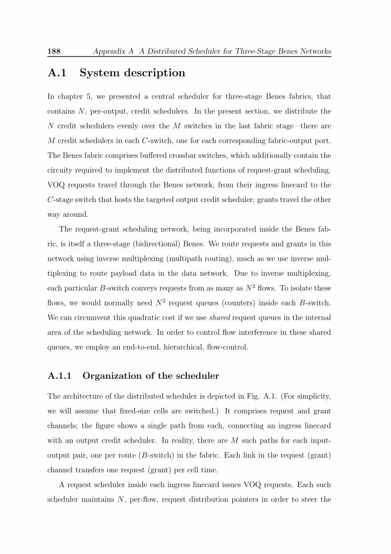
188 Appendix A A Distributed Scheduler for Three-Stage Benes Networks
A.1 System description
In chapter 5, we presented a central scheduler for three-stage Benes fabrics, that
contains N , per-output, credit schedulers. In the present section, we distribute the
N credit schedulers evenly over the M switches in the last fabric stage –there are
M credit schedulers in each C-switch, one for each corresponding fabric-output port.
The Benes fabric comprises buffered crossbar switches, which additionally contain the
circuity required to implement the distributed functions of request-grant scheduling.
VOQ requests travel through the Benes network, from their ingress linecard to the
C-stage switch that hosts the targeted output credit scheduler; grants travel the other
way around.
The request-grant scheduling network, being incorporated inside the Benes fab-
ric, is itself a three-stage (bidirectional) Benes. We route requests and grants in this
network using inverse multiplexing (multipath routing), much as we use inverse mul-
tiplexing to route payload data in the data network. Due to inverse multiplexing,
each particular B-switch conveys requests from as many as N 2 flows. To isolate these
flows, we would normally need N 2 request queues (counters) inside each B-switch.
We can circumvent this quadratic cost if we use shared request queues in the internal
area of the scheduling network. In order to control flow interference in these shared
queues, we employ an end-to-end, hierarchical, flow-control.
A.1.1 Organization of the scheduler
The architecture of the distributed scheduler is depicted in Fig. A.1. (For simplicity,
we will assume that fixed-size cells are switched.) It comprises request and grant
channels; the figure shows a single path from each, connecting an ingress linecard
with an output credit scheduler. In reality, there are M such paths for each input-
output pair, one per route (B-switch) in the fabric. Each link in the request (grant)
channel transfers one request (grant) per cell time.
A request scheduler inside each ingress linecard issues VOQ requests. Each such
scheduler maintains N , per-flow, request distribution pointers in order to steer the

A.1 System description 189
requests from each flow evenly across the M available paths. The requests from
the different flows are multiplexed on intermediate (A→B, B→C) links in the re-
quest channel, and sink in per-flow request queues (counters), in front of the targeted
credit scheduler –there are M×N request counters inside each C-switch. The request
schedulers ensure that the VOQ requests that they issue can be accommodated by
the respective request counter; as in section 5.2.6, the per-flow grants received at
the ingress linecards inform them of the space released in these counters. Through
this end-to-end flow control, the number of pending requests from each flow is upper
bounded by u, i.e. the number of requests that can be accommodated in a request
counter. The aggregate number of requests that are pending inside the scheduling
network and are destined to a given fabric-output is upper bounded by N · u. Ef-
fectively, if λc denotes the cell rate on a link –this is equal to the peak grant rate
per output–, the aggregate number of requests issued to a given fabric-output during
a time interval, T , from any number of inputs, is upper bounded by T · λc + N · u;
similarly, the aggregate number of requests issued towards all outputs in a particular
C-switch is upper bounded by M · T · λc + M ·N · u.
Each output credit scheduler maintains N , per-flow distribution pointers, and M
credit counters, one for each crosspoint in front of the corresponding fabric-output.
Credit schedulers operate independently, serving (inputs’) request counters as de-
scribed in section 5.2.6. Since we assume buffered crossbar switches, when a credit
scheduler serves an input, it must choose a particular B-switch (route), and reserve
space in the corresponding crosspoint buffer. This route is pointed by the distribution
pointer of the served flow. Subsequently, the credit scheduler issues a grant to the
served input. (We use the coordinated load distribution method described in section
5.2.4 in order to eliminate route identifiers from grant messages.) This grant will be
routed through the path (B-switch) in which the credit scheduler reserves crosspoint
buffer space for the corresponding cell2.
2We do not need separate per-flow grant distribution pointers.
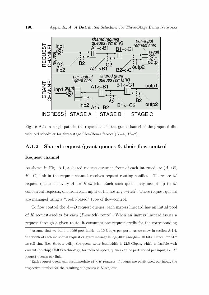
190 Appendix A A Distributed Scheduler for Three-Stage Benes Networks
SS
S
S
RE
QU
ES
TC
HA
NN
EL
GR
AN
TC
HA
NN
EL
C2B2
credit
A2 B2
STAGE B STAGE C
inp1 grant
outp1
inp2
outp1
outp2
inp1
inp2
requ
est
INGRESS STAGE A
per−inputrequest cnts
per−outputgrant cnts queues (sz: M*K)
B1<−C2A1<−B2
outp2
A1<−B1 B1<−C1
B2−>C1
B1−>C1
A2−>B1
A1−>B1
shared requestqueues (sz: M*K)
shared grant
Figure A.1: A single path in the request and in the grant channel of the proposed dis-
tributed scheduler for three-stage Clos/Benes fabrics (N=4, M=2).
A.1.2 Shared request/grant queues & their flow control
Request channel
As shown in Fig. A.1, a shared request queue in front of each intermediate (A→B,
B→C) link in the request channel resolves request routing conflicts. There are M
request queues in every A- or B-switch. Each such queue may accept up to M
concurrent requests, one from each input of the hosting switch3. These request queues
are managed using a “credit-based” type of flow-control.
To flow control the A→B request queues, each ingress linecard has an initial pool
of K request-credits for each (B-switch) route4. When an ingress linecard issues a
request through a given route, it consumes one request-credit for the corresponding
3Assume that we build a 4096-port fabric, at 10 Gbp/s per port. As we show in section A.1.4,
the width of each individual request or grant message is log24096+log264= 18 bits. Hence, for 51.2
ns cell time (i.e. 64-byte cells), the queue write bandwidth is 22.5 Gbp/s, which is feasible with
current (on-chip) CMOS technology; for reduced speed, queues can be partitioned per input, i.e. M
request queues per link.4Each request queue can accommodate M ×K requests; if queues are partitioned per input, the
respective number for the resulting subqueues is K requests.

A.1 System description 191
request queue in the downstream A-switch. This request-credit must return to the
linecard when the request departs from the A-switch. Similarly, each A-switch has a
pool of K request-credits for each B/C switch-pair. When it forwards a request, it
consumes one credit for the corresponding B/C switch-pair, that must return when
the request departs from the B-stage. The requests can freely depart from stage B,
since space for them in stage C has already been reserved via the end-to-end flow
control. Because there is no backpressure on the shared request queues in front of
B→C request links, HOL blocking cannot appear in them.
However, if the instant request rate, from all inputs, towards a particular C-switch
exceeds M · λc –i.e. the aggregate capacity of the B→C request links connecting to
a C-switch– the request queues in front of the corresponding B→C request links
will grow. In the mid- to long-term, inputs will stop sending requests towards the
“hotspot” C-switch at this excessive rate, since the aggregate request rate for this C-
switch will be equalized to the aggregate rate at which the corresponding outputs issue
grants, i.e. ≤ M ·λc. Despite this eventual throttling, the overshooted B→C request
queues may remain full, and exert (indiscriminate) backpressure on the shared A→B
request queues. Effectively, HOL blocking may develop inside these backpressured
queues, spreading congestion out. As we show in section A.2.2, this problem can be
solved by speeding up the B→C request links by some small factor (e.g. ×1.1 or even
less)5.
Grant channel
The grant channel (reverse path) contains a shared grant queue in front of each
intermediate (C→B, B→A) link. There are M grant queues in every B- or A-switch.
These grant queues are managed using a “credit-based” type of flow control. Each
credit scheduler has an initial pool of K grant-credits for each B-switch6. When it
5Considering that in an actual implementation requests can be routed from B-switches to C-
switches through the corresponding data links, this ×1.1 speedup can be realized by allowing requests
to consume a slightly higher percentage of that links’ capacity.6Each shared grant-queue can accomodate M × K grants; if grant queues are partitioned per
input for reduced queue speed, the respective number for the resulting subqueues is K grants.

192 Appendix A A Distributed Scheduler for Three-Stage Benes Networks
issues a grant through a given route, it consumes one grant-credit for that route7. In
order to prevent overflow in the grant queues that reside in B-switches, each C-switch
maintains an initial pool of K grant-credits for each B/A switch-pair. Grants can
depart from the C-switch only when a grant-credit for the targeted B/A switch-pair
is available.
We assume per-flow grant counters in front of the links that convey grants from
A-switches to ingress linecards –there are M×N counters inside each A-switch. These
grant counters do not require an explicit flow control, since by limiting the number
of pending per-flow requests, we also limit the number of pending per-flow grants8.
Independent input grant schedulers serve the per-flow grant counters, and issue grants
to the ingress linecards. Due to multipath grant routing, consecutive grants for the
same flow may be routed out-of-order to the ingress side, but there is no problem
with that since the per-flow grants are interchangeable with each other.
A.1.3 Cell injection
Upon receiving a grant, the ingress linecard injects the corresponding cell as described
in section 5.2.6. The crosspoint buffers in stages A and B exert credit-based back-
pressure in order to prevent overflow; the crosspoint buffers in the C-stage do not
exert backpressure. As pointed out in section 4.2.3, even though the backpressure
in the first fabric stages is indiscriminate, it does not hurt performance. The rese-
quencing circuit in each egress linecard determines when a cell is in-order. For each
in-order cell, a credit is sent back to the corresponding credit scheduler. As described
in section 4.3.2, this method bounds the size of the reorder buffers.
7Effectively, one additional condition must also be met for a credit scheduler to be able to issue
a new grant: grant-credits must be available for the route pointed by the distribution pointer of the
candidate flow.8It is not a strict requirement to use per-flow grant counters; if desired, these can be replace by
shared grant queues, managed in the same fashion with B→A grant queues.

A.1 System description 193
inp:log2(N)route:log2(M) inp:log2(M)
REQUESTS
GRANTS
B−s
witc
h
C−s
witc
h
A−s
witc
h outp:log2(N)outp:log2(N)
inp:log2(M)outp:log2(N) outp:log2(M)
inp:log2(N)outp:log2(N)
outp:log2(M)
linec
ard
ingr
ess
Figure A.2: Request and grant messages convey only the ID of the respective flow; the
information needed to identify a flow changes along the route of request-grant messages.
A.1.4 Request/grant messages & their storage cost
Figure A.2 depicts the size of the request and grant messages that implement
the request-grant backpressure protocol. The information required to identify a flow
changes from hop to hop. The requests that go out from an ingress linecard indicate
the targeted fabric-output port, and the path (B-switch) in the request channel; the
grants sent to ingress linecards identify the fabric-output port that they come from.
At a link between an A-switch and a B-switch, there are M inputs combined with N
outputs to identify and separate from each other; symmetrically, at a link between a
B-switch and a C-switch, there are M outputs combined with N inputs to identify
and separate from each other. Effectively, the size of a request or grant message is
always smaller than log2M + log2N bits.
Each A- or B-switch has M request queues, and each such queue has a capacity
of M ·K requests. Assume that M= 64 (N= 4096), and that K= 32 (note9). Then,
each queue will need to store 2048 requests of 18 bits each. Hence, we need 36 Kbits
per request queue, or 2.25 Mbits for all request queues in a switch. With 6 transistors
per memory bit, the number of transistors consumed for request storage per switch is
roughly equal to 13.5 M. Each B-switch additionally contains M grant queues, hence
it needs a total of 4.5 Mbits (27 M transistors) for both request and grant storage.
Each C- or A-switch contains M ·N request or grant counters, respectively. For
9In general, K must be set according to the local round-trip time between the nodes participating
in the request or grant queue flow control; the value of 32 that we consider here is rather pessimistic.

194 Appendix A A Distributed Scheduler for Three-Stage Benes Networks
our example 4096-port fabric, there are 256 K counters per switch. Assuming that
each counter can store up to 32 requests (u= 32), the counter width will be 5 bits;
for 25 transistors per counter bit, this yields 256 · 5 · 25 K ≈ 32 M transistors per
switch. To reduce the transistor count, several counters can be implemented in an
SRAM block, with external adders for increments and decrements.
A.2 Performance simulation results
In this section we evaluate the performance of the distributed scheduler under hotspot
traffic. All schedulers in the fabric and the scheduling network implement the round-
robin discipline; to improve “desychronization”, the output credit schedulers imple-
ment the random-shuffle round-robin discipline, presented in section 3.7. The data
round-trip time is set to 12 cell times, and the crosspoint buffer size is set to 12 cells.
Parameters u (i.e. the capacity of each request counter) and K (i.e. 1M
-th of the
capacity of each request or grant queue) are both set to 32.
A.2.1 Randomly selected hotspots
Figure A.3 depicts the delay of well-behaved flows in the presence of a varying number
of other congested outputs (hotspots). Hotspots are randomly selected among the
fabric outputs, and each one receives 100% traffic uniformly from all inputs. For
comparison, we also plot cell delay when no hotspot is present, denoted by h/0, and
the OQ delay. To see how well the present system isolates flows, observe that the
delay of h/2 –i.e. the delay of well-behaved flows in the presence of two (2) congested
outputs– is virtually identical to that of h/0. If the well-behaved flows were subject to
backpressure signals coming from queues that feed oversubscribed outputs, or if the
scheduling network suffered from the requests of congested flows, the delay of well-
behaved flows could probably grow without bound, even at very moderate loads. The
delay in Fig. A.3 increases with the number of hotspots, because the hotspot traffic
increases the contention along the shared paths inside the fabric and the scheduling

A.2 Performance simulation results 195
no hotspot (h/0)
OQh/32
h/16
50 hotspots (h/50)
h/2
0.01 0.1 0.2 0.3 0.4 0.5 0.6 0.7 0.8 0.9 1normalized load at non−hotspot destinations
0.1
1
10
100
500av
erag
e de
lay
of c
ells
des
tined
to n
on−h
otsp
ots
(cel
l tim
es)
Figure A.3: Delay of well-behaved flows in the presence of hotspots; h/• specifies the
number of hotspots, e.g. h/4 corresponds to four hotspots. Fixed-size cell Bernoulli arrivals;
64-port fabric, b= 12 cells, RTT= 12 cell times. Only the queueing delay is shown, excluding
all other fixed delays.
network. This effect was also observed in the centralized fabric scheduler (see section
5.4.3). The delay of h/50 at 0.1 input load is approximately equal to the delay of
h/0 at 0.8 input load; this happens because in h/50, at 0.1 load for the non-hotspot
destinations, the effective load at which each input injects traffic is ≈ 0.8.
Hence, we see that the system behaves very well in the presence of hotspots,
because there is no HOL blocking inside B→C request queues. But, in principle,
HOL blocking can appear inside the request queues in the A-stage.
A.2.2 Congested B→C links: problem & possible solutions
A B→C request queue may fill, either occasionaly, due to unlucky routing decisions,
or permanently, when the combined request rate, from all inputs, for a set of outputs
in a C-switch, say switch C1, exceeds the aggregate capacity of request links Bi→C1,
i ∈ [1, M ], i.e. M · λc. That request rate can only be sustained in a transient state,
since in the mid- to long-term, the aggregate request rate for any given output is

196 Appendix A A Distributed Scheduler for Three-Stage Benes Networks
bounded by the rate that this output issues grants, i.e. λc, which is equal to one
grant (request) per cell time; hence, the aggregate long-term request rate for all
outputs in switch C1 is upper bounded by M · λc.
But during a time interval T ≥M · u cell times, the N ingress linecards may send
a total of M · T · λc + N ·M · u requests towards switch C1; from this volume of
requests, only M ·T ·λc can make it inside switch C1, because the aggregate capacity
of the links conveying requests to C1 is M · λc. The remaining N ·M · u requests
will have to wait in the request queues in front of the M request links connecting to
C1. If these queues cannot hold this amount of requests (i.e. if the aggregate number
of requests that fit in each B→C request queue is below N · u), they will fill, thus
exerting indiscriminate backpressure on the shared request queues in the A-stage.
This problem did not appear in the previous experiments, because the aggregate
request rate for any C switch was always safely below M · λc: in any experiment,
at least one output of each C switch was not overloaded. Thus, the B-stage request
queues only rarely exerted backpressure on the request queues in the A-stage. Effec-
tively, the A-stage request queues drained at the rate that they filled, thus no HOL
blocking appeared inside them also. But this only happened by chance, in section
A.2.1.
In the following experiment, we overload the outputs 1 to 8 in a 64-port fabric, in
order to overload the request links Bi→C1, i ∈ [1, 8]. Figure A.4, plots the delay of
cells destined to non hotspot outputs, (i) when no hotspot is present, (ii) when each
one of the eight hotspots is loaded with 100% traffic, and (iii) when each one of the
eight hotspots is loaded with 300% traffic –in this case, the maximum load at each
of the non-hotspot outputs is approximately (64-3· 8)/56 ≈ 0.7. As can be seen in
the figure, well-behaved flows suffer considerably under these stressing conditions. As
described above, this happens due to HOL blocking that develops in the first stage
of the request channel: Requests destined to C1 are severely delayed inside A→B
request queues by downstream backpressure, thus blocking other requests, for lightly
loaded C-switches, which wait behind them in these request queues, or wait in the
A.2 Performance simulation results 197
all outputs in C1 are overloaded
100% load per hotspot
300% load per hotspot
no hotspot
B−>C request link rate = 1 req. per cell time 0.1 0.1 0.2 0.3 0.4 0.5 0.6 0.7 0.8 0.9 1
load at non−hotspots destinations
1
10
100
1000
aver
age
dela
y of
cel
ls d
estin
ed to
non
−hot
spot
s (c
ell−
times
)
Figure A.4: Delay of well-behaved flows in the presence of hotspots. Rate of B→C request
links equal to λc (1 requests / cell time, per link); 64-port fabric. Hotspots are the outputs
of switch C1. Fixed-size cell Bernoulli arrivals; b= 12 cells, RTT= 12 cell times. Only the
queueing delay is shown, excluding all other fixed delays. For some of the delays shown we
have not achieved the desired confidence intervals.
ingress linecards because there are no request-credits for them to move to the first
stage –the congested request queues hog these request-credits.
To avoid the performance degradation caused by overloaded B→C1 links, we
can (a) size the request queues in front of Bi→C1 links, i ∈ [1, M ], so that these
queues never fill up permanently. (In the last experiment, the size of each request
queue is M ·K, or M · u since in this experiment K = u = 32.) If each such queue
can hold ≥ N · u requests, then the requests for C1 that are pending inside the
request channel will fit in the request queues in front of B→C1 links; hence, these
queues will only sporadically exert backpressure (due to unlucky routing), drastically
diminishing in this way the HOL blocking effect inside the A→B request queues.
However, increasing by (at least) M times the request buffer storage in each B-
switch, as required by this method, is not practical. Another solution is (b) to limit
the number of requests that each ingress linecard may have pending towards each
particular C-switch. If each linecard is allowed up to u pending requests per C-
switch, we can achieve the same goal as method (a), but with the existing request

198 Appendix A A Distributed Scheduler for Three-Stage Benes Networks
300% load per hotspot
B−>C request link rate= 1.1 req. per cell time
100% load per hotspotno hotspot
all outputs in C1 overloaded
0.1 0.1 0.2 0.3 0.4 0.5 0.6 0.7 0.8 0.9 1load at non−hotspots destinations
1
10
100
to n
on−h
otsp
ots
(cel
l−tim
es)
aver
age
dela
y of
cel
ls d
estin
ed
Figure A.5: Delay of well-behaved flows in the presence of hotspots. Rate of B→C request
links equal to 1.1·λc (1.1 requests / cell time, per link); 64-port fabric. Hotspots are the
outputs of switch C1. Fixed-size cell Bernoulli arrivals; b= 12 cells, RTT= 12 cell times.
Only the queueing delay is shown, excluding all other fixed delays.
buffer storage (assuming that K = u). However an ingress linecard may consume its
allowable requests towards a particular C-switch, sending them to congested outputs,
thus not being able afterwards to request other, possible lightly loaded destinations
in the same C-switch. A different approach is (c) to use separate request queues
for the flows destined to different C-switches: the request queues in the A-stage
must be organized per C-switch, and they must exert discriminative backpressure on
the ingress linecards. This method requires significant modifications in the request
channel, which may increase cost. The following solution is much simpler.
What we essentially need to achieve is to drain the filled request queues in front of
B→C1 links. If the capacity of B→C1 request links is slightly higher than the long-
term demand for these links, the request queues will almost always be empty: they
may temporarily fill in the start of a congestion epoch, but they will subsequently
drain. In Fig. A.5, we repeat the last experiment (see Fig. A.4), but we set the rate
of each B→C request link equal to 1.1·λc, i.e. a speedup of just 10% in request rate.
All other request or grant links in the scheduling network operate at their default

A.2 Performance simulation results 199
rate, λc. As can be seen in the figure, with this marginal speedup on B→C request
links, the presence of hotspots does not affect the well-behaved flows.
We observed that the request queues in front of B→C1 links fill up in the beginning
of the experiment (which corresponds to the onset of a congestion epoch) and drain
shortly after. While the queues are filled, the delay of well-behaved might increase.
The rate that the filled queues drain, thus the duration of the transient, depends on
the value of speedup used. Considering that in an actual implementation, requests
can be forwarded from B- to C-switches through the corresponding data links, which
have an order of magnitude higher capacity than 1 request notice (log2 N+log2 M
bits) per cell time, the duration of such transients can be made arbitrarily short (or
even null).

200 Appendix A A Distributed Scheduler for Three-Stage Benes Networks

Appendix B
Performance Simulation
Environment
An event-driven simulation model was developed in order to verify the systems studied
in this thesis, and to evaluate their performance.
B.1 Simulator
The simulator uses an event heap, implemented using the priority queue template
from the SGI Standard Template Library (STL), in order to store simulation events,
and to pull them out in increasing time order. Design models are built at the system-
architecture level. The basic level of abstraction is the contention point: control
and data packets arrive at contention points, where they are queued according to a
queueing policy. At each contention point, a scheduler visits the queues according to
a service discipline; the head-of-line packet of the selected queue is served either in
constant time (e.g. a cell time, or a minimum-packet time) or in time proportional to
its size. Contention points are scheduled only when there are no more present-time
events inside the heap1.
1In this way, we avoid race conditions, as scheduling decisions do not depend on the relative order
at which concurrent events (e.g. packet arrivals at a given contention point) are pulled out of the
heap.
201

202 Appendix B Performance Simulation Environment
B.2 Traffic patterns
Unless otherwise noticed, packet arrivals are identical and independently distributed
(i.i.d.) across all inputs. To ensure that traffic input sources are independent from
each other, a separate random number generator, initialized with a different seed, is
associated with every input2. A traffic source can be characterized by two parame-
ters: (a) the packet arrivals type, which determines the way that packet arrivals are
distributed in time, and (b), the output selection function, which determines packets’
output destination.
B.2.1 Packet arrivals
For fixed-size cell traffic, we use two different arrival types: smooth and bursty. For
variable-size packet traffic, we use Poisson arrivals.
Smooth cell arrivals
Smooth cell arrivals are based on Bernoulli trials. Assume that the target normalized
load of the switch is ρ. In each cell time, we pull a uniform random variable, z
∈ (0 : 1), and we trigger a new cell arrival if and only if z ≤ ρ.
Bursty cell arrivals
Bursty cell arrivals are based on a two-state (ON/OFF) Markov chain. ON periods
(consecutive, back-to-back cells arriving at an input for a given output) last for at
least one (1) cell time, whereas OFF periods may last zero (0) cell times, in order to
achieve 100% loading of the switch. The state probabilities are calibrated so as to
achieve the desirable load, giving exponentially distributed burst length around the
average indicated in any particular experiment. The details of the traffic model used
can be found in [Minkenberg01] (pp. 194-195).
2The “erand48()” function is used in order to generate pseudo-random numbers, uniformly dis-
tributed in the interval (1, 0).

B.2 Traffic patterns 203
Poisson packet arrivals
In Poisson packet arrivals, packets’ inter-arrival times are exponentially distributed.
We generate exponential variates using the inverse transform method [Ross01].
B.2.2 Output selection
The output selection function determines packets’ destination. When arrivals are
smooth, the output selection function is executed for every new packet; when arrivals
are bursty, all packets in a burst have the same destination as the burst’s head packet.
Uniformly-destined traffic
Under uniformly-destined traffic, all input-output connections i→j have the same
load. Given the normalized switch load, ρ, each connection i→j carries a load of
(1/N)×ρ. For output selection, we pick an integer, uniform, random variable z ∈[1, N ].
Unbalanced traffic
In unbalanced traffic, some input-output connections are more loaded than the rest.
As in [Rojas-Cessa01], the unbalance degree is controlled by w, which ranges in [0, 1]:
the normalized traffic load ρi,j, from input i to output j is given by w + 1−wN
, when
i = j, and by 1−wN
, otherwise. Traffic is uniformly-destined when w= 0, and completely
unbalanced –i.e. persistent i→i, i ∈ [1, N ], connections– when w= 1. To determine
the output of a packet arriving at input i, we pull a uniform random variable, z
∈(0, 1); if z < w, the destination of the packet is i; otherwise, it is uniformly selected
among all output ports.
Diagonal traffic
Diagonal traffic is another type of unbalanced traffic. Each input i hosts two active
flows, flow i→i, and i→(i+1) mod N . The former flow consumes two thirds (2/3) of
the incoming load, and the latter flow consumes the remaining one third (1/3). For
204 Appendix B Performance Simulation Environment
output selection, when a packet arrives at input i, we pull a uniform random variable,
z ∈ (0, 1); if z ≤ 2/3, the destination of the packet is i; otherwise, it is (i + 1) mod
N .
Hotspot traffic
Under hotspot traffic, each destination belonging to a designated set of K “hotspots”
receives a normalized load l, uniformly from all sources; the rest of the destinations
receive a smaller load. In most experiments presented in this thesis, l= 1. When
a packet arrives, we pull a uniform random variable, z ∈ (0, 1); if z < l · K/N , the
destination of the packet is uniformly selected among the hotspot outputs; otherwise,
it is uniformly selected among the non-hotspots. To generate a load ρ for the non-
hotspot outputs, the effective load at which each input generates traffic is ρ · (N −K)/N + l ·K/N .
B.3 Statistics collection
Each simulation experiment consists of two successive phases: the warm-up phase
and the statistics collection phase. Delay and throughput samples are collected only
during the statistics collection phase. The transition to this phase is signaled when k
packets have been forwarded to fabric-outputs. Parameter k is ≥ 10K, and increases
with the input load, approaching 4M when the input load approaches the saturation
point of the system. These number are for 32-port switches, and for smooth or Poisson
packet arrivals. In simulations of switches with number of ports, N , greater than 32,
k increases proportionally to N/32: k ← k ·N/32. In simulations using bursty traffic,
k also increases proportionally to the average bursty size (abs): k ← k · 3, when abs
= 12, and k ← k · 3· abs/12, when abs > 12.
The statistics collection phase is divided into successive collection intervals, each
one lasting for m sampled packets3. In each interval we compute the mean packet
delay and the throughput of the system. We report the average of these measurements
3Parameter m is at least 10000, and is updated similarly to k.
B.3 Statistics collection 205
in at least 30 intervals. The simulation terminates [Ross01] either when more than
60 intervals have elapsed, in which case the system is considered unstable, or when
with 95% confidence, the “true value” of the performance metric measured is within
X% from our estimate (X= 10 for delay, X=1 for throughput). Every simulation
experiment is run at least 3 times using different random seeds.


