
NICE Research Journal, Vol.13 No.4 (2020): October-December ISSN: 2219-4282
82
Full Length Article Open Access
Stand Still and Do Nothing: COVID-19 and Stock Returns and Volatility
Muhammad Akbar1, Aima Tahir2, Syeda Faiza Urooj3
1Senior Lecturer, Birmingham City Business School, Birmingham City University, UK 2University of Reading, UK 3Assistant Professor, Department of Commerce, FUUAST Islamabad
A B S T R A C T
We examine the intraday returns and volatility in the US equity market amid the COVID-19
pandemic crisis. Our empirical results suggest an increase in volatility over time with mostly
negative returns and higher volatility in the last trading session of the day. Our Univariate
analysis reveals structural break(s) since the first trading halt in March 2020 and that failure to
account for this may lead to biased and unstable conditional estimates. Allowing for time-varying
conditional variance and conditional correlation, our dynamic conditional correlation tests suggest
that COVID-19 cases and deaths are jointly related to stock returns and realised volatility.
Key words: COVID-19, Stock Returns and Volatility, DCC, Multivariate GARCH.
1. INTRODUCTION
Financial markets have experienced unprecedented levels of volatility in March
2020 since the outbreak of the COVID-19 global pandemic. The extent of the panic can
be gauged from the US equity market where trading was halted on the New York Stock
Exchange (NYSE) on the 9th, 12th, 16th, and 18th of March as the S&P500 dropped1.
The VIX volatility index increased from 17.08 on February 21 to 82.70 on March 16 after
the World Health Organisation (WHO) declared COVID-19 a global pandemic on March
11, 20202. Stock prices fell 30% compared to the 34% drop of the 1987 market crash
(Siegel, 2020). It has led to the end of the record 11 years longest bull market in mid-
March3. In May and June, the VIX volatility index is on average double the level it was in
1 https://graphics.reuters.com/USA-MARKETS/0100B5L144C/index.html 2 https://www.who.int/emergencies/diseases/novel-coronavirus-2019/events-as-they-happen 3 https://crsreports.congress.gov/product/pdf/IN/IN11309
Address of Correspondence Syeda Faiza Urooj [email protected]
Article info Received Oct 16, 2020 Accepted Nov 26,2020 Published Dec 30,2020

NICE Research Journal, Vol.13 No.4 (2020): October-December ISSN: 2219-4282
83
January 20204. Such high levels of volatility may only favour volatility traders
particularly in the options markets; however, it is detrimental for risk-averse investors
(Chance and Brooks). It must be noted that it is the first time that such a crisis in financial
markets in peacetime is induced by a simultaneous disruption to both supply and demand
(Siegel, 2020).
The emerging literature on the COVID-19 pandemic and its implications for
financial markets is still at an early stage. These studies have focused mostly on volatility
and the aspects of the COVID-19 pandemic such as new cases, the number of daily
deaths, sentiments, media coverage, etc. (Baig et al., 2020; Haroon and Rizvi, 2020;
Onali, 2020; Papadamou et al., 2020; Baker et al., 2020). Most of these studies have
provided empirical evidence in support of the impact of the COVID-19 crisis (cases and
deaths) on stock returns and volatility (Baig et. Al., 2020; Haroon and Rizvi, 2020; Mirza
et al., 2020; Yousaf, 2020; Zhang et al, 2020). However, these studies have mainly
analysed daily data on returns; have a relatively shorter sample period post the peak of
the market volatility in March 2020.
Volatility has broad implications for trading, asset pricing, investment, and risk
management. COVID-19 pandemic-induced volatility leads to a shift of informed trading
activity to dark pools from lit avenues (Ibikunle and Rzayev, 2020). This has significant
implications for asset pricing particularly in terms of price discovery due to loss of
informational efficiency (Ibikunle and Rzayev, 2020). The conditional correlation
between stock returns of both financial and non-financial firms across countries increased
during the COVID-19 pandemic period that implies financial contagion leading to higher
optimal hedge ratios and hence higher hedging costs (Akhtaruzzaman et al., 2020). The
use of daily stock price data to measure stock returns and volatility may not be
appropriate particularly given high-frequency trading (HFT) based on algorithms that
closely monitor changes in stock prices and the resulting consequences for market
liquidity (Anagnostidis and Fontaine, 2020). The intra-day trend and patterns in both
stock returns and volatility have significant implications for market timing and trading
4 http://www.cboe.com/vix
NICE Research Journal, Vol.13 No.4 (2020): October-December ISSN: 2219-4282
84
activities. This is particularly significant given the circuit breaker rules in place on the
NYSE where trading halt do not apply after 3:25 p.m. if the S&P500 drops below 7%5.
In this study, first, we analyse the intraday day i.e. 10 minutes S&P500 index
data accounting for the evolution of the realised volatility and its trends and patterns
during different trading hours over each trading day. Then we investigate the volatility in
the market using the intraday returns using univariate GARCH models. However, unlike
the extant literature we use the log-likelihood ratio to choose different GARCH
specifications for before and after the first trading halt (i.e. 9th March 2020) as well as
the full sample period i.e. 2nd January to 5th June 2020. We do not use Exponential
GARCH given stationarity of the time series of intraday returns6. Finally, we analyse the
relationship between stock returns and volatility with COVID-19 cases and deaths using
the Dynamic Conditional Correlation (DCC) multivariate GARCH. Unlike the
conventional multivariate GARCH, the DCC multivariate GARCH directly parameterise
conditional correlations. Another advantage is that the number of series considered in the
analysis has no role in the determination of the number of parameters estimated (Engle,
2002).
2. DATA AND EMPIRICAL METHODS
For our empirical analysis and evaluation, we have used the S&P500 index as a
benchmark proxy of US equity prices. Our sample covers the intraday S&P500 index
values at the 10-minute interval from 2nd January to 5th June 2020 obtained from
Bloomberg. Data on confirmed COVID-19 total cases, new cases, total death, and new
death in the US is obtained from Oxford COVID-19 Government Response Tracker
(OxCGRT)7.
We calculate the logarithmic 10 minutes return ( ) as:
(1)
5 https://www.nyse.com/markets/hours-calendars 6 Different specifications, including ARFIMA, were considered in each case and selection was
based in each case on the Log-likelihood ratio. 7 https://www.bsg.ox.ac.uk/research/research-projects/coronavirus-government-response-
tracker#data

NICE Research Journal, Vol.13 No.4 (2020): October-December ISSN: 2219-4282
85
Where the current 10-minute is the value of the S&P500 index and is
the lagged 10-minute value of the S&P500 index. We calculate the realised volatility for
any trading day ( ) as the sum of the squared (i.e. for each
day. We then divided the trading day into four equal 2 hours’ sessions and calculate the
realised volatility for each session similarly to ascertain the pattern and trends in realised
volatility and returns over the day.
First, we use standard univariate GARCH to analyse the conditional volatility of
the intraday returns and assess different specifications in both mean and variance
equations to choose the best fit based on the log-likelihood ratio. The conditional mean
and variance equations in the standard GARCH model are given in equation 2 and 3 as:
(2)
(3)
Where is the intercept term, and are the autoregressive and
moving average components of the conditional mean equation and is a residual term
of the mean equation. Further, is the conditional variance of , is the alpha
(intercept) term while q and p represent the lag order of the squared residual term ( )
and the conditional variance ( ) with and estimated coefficients respectively in
the conditional variance equation. We selected the best fit from our estimations of the
specifications (in mean and variance) of the standard GARCH for the full sample as well
as before and after 9th March 2020 subsample periods based on the log-likelihood
criterion8.
We use the DCC, multivariate GARCH approach to measure the impact of the
COVID-19 pandemic crisis on stock returns and volatility. It is a two steps process; the
first step is a series of univariate GARCH estimates and the second step involves
8 We divided the sample based on the first trading halt on the opening of trading on the 9th of
March 2020. So we have the first period before the first trading halt from 2nd January to 6th March
2020 and then from 9th March to 5th June 2020 that includes the extreme volatility from 9th March
to the last week of trading in March.
NICE Research Journal, Vol.13 No.4 (2020): October-December ISSN: 2219-4282
86
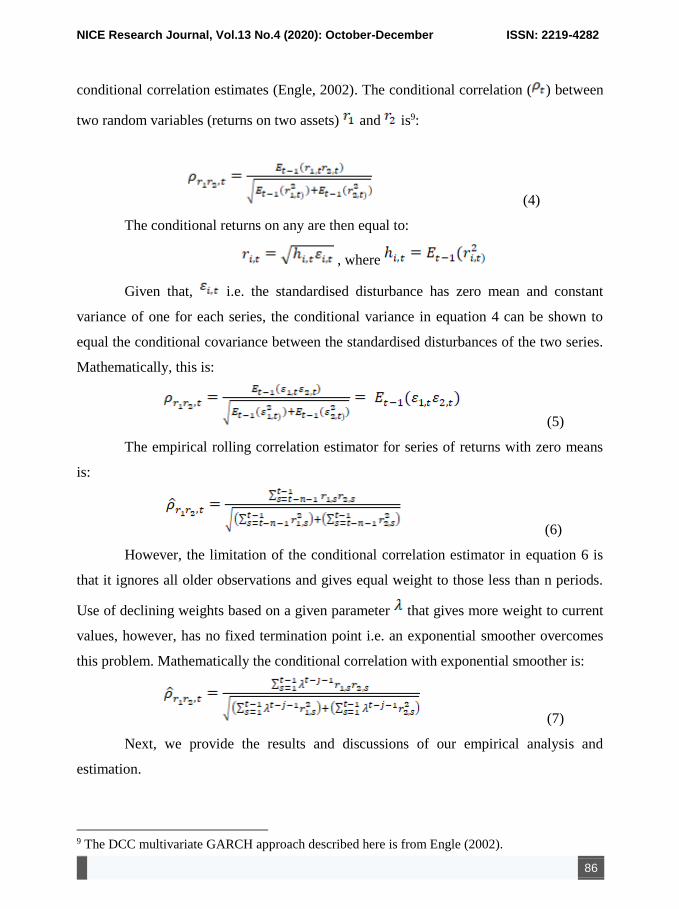
conditional correlation estimates (Engle, 2002). The conditional correlation ( ) between
two random variables (returns on two assets) and is9:
(4)
The conditional returns on any are then equal to:
, where
Given that, i.e. the standardised disturbance has zero mean and constant
variance of one for each series, the conditional variance in equation 4 can be shown to
equal the conditional covariance between the standardised disturbances of the two series.
Mathematically, this is:
(5)
The empirical rolling correlation estimator for series of returns with zero means
is:
(6)
However, the limitation of the conditional correlation estimator in equation 6 is
that it ignores all older observations and gives equal weight to those less than n periods.
Use of declining weights based on a given parameter that gives more weight to current
values, however, has no fixed termination point i.e. an exponential smoother overcomes
this problem. Mathematically the conditional correlation with exponential smoother is:
(7)
Next, we provide the results and discussions of our empirical analysis and
estimation.
9 The DCC multivariate GARCH approach described here is from Engle (2002).

NICE Research Journal, Vol.13 No.4 (2020): October-December ISSN: 2219-4282
87
3. EMPIRICAL RESULTS
Table 1 presents the descriptive statistics on the 10-minute intraday returns for
January through May 2020 and the full sample period. The returns are negative in the
first three months and then positive for April and June. The volatility as measured by
standard deviation is rising from January to March (0.278% to 0.984%) and then falling
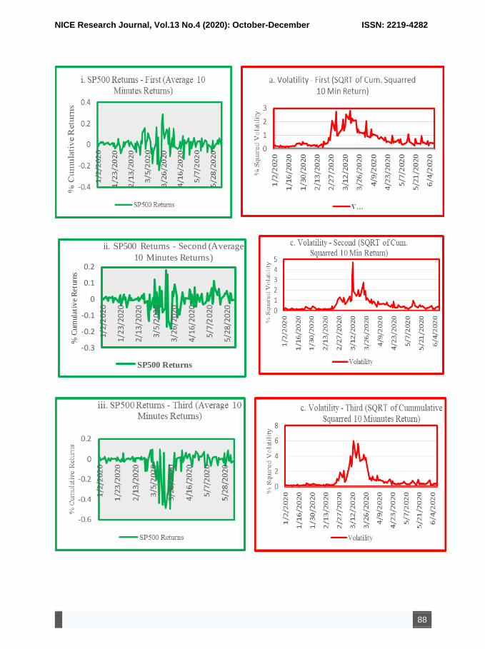
onward (0.382% in May). Figure 1 depicts the S&P500 daily average 10-minute returns
and the square root of the cumulative squared 10-minute returns as the measure of
volatility. Overall, this trend in returns and volatility coincides with the progression of the
COVID1-9 pandemic crisis. The relative stability after March 2020 is partially due to the
US government policy responses to stabilise the economy and Federal Reserve measures
for financial stability.
Table 1
Descriptive Statistics on Intraday Returns
Mean Std.Dev Min Max
Jan-20 -0.002 0.278 -1.622 1.623
Feb-20 -0.012 0.357 -1.791 2.581
Mar-20 -0.017 0.984 -8.936 8.028
Apr-20 0.015 0.562 -2.541 5.488
May-20 0.006 0.382 -1.754 4.066
Full Sample 0.000 0.574 -8.936 8.028
Figure. 1. S&P500 Cumulative Daily Returns and Volatility
NICE Research Journal, Vol.13 No.4 (2020): October-December ISSN: 2219-4282
88
-0.3
-0.2
-0.1
0
0.1
0.2
1/2
/20
20
1/23
/202
0
2/13
/202
0
3/5
/20
20
3/26
/202
0
4/16
/202
0
5/7
/20
20
5/28
/202
0
% C
um
ula
tiv
e R
eturn
s
ii. SP500 Returns - Second (Average
10 Minutes Returns)
SP500 Returns

NICE Research Journal, Vol.13 No.4 (2020): October-December ISSN: 2219-4282
89
Figure 2. S&P500 Intraday Returns Volatility in Sessions Overtime
Figure 2 presents the S&P500 average 10-minute returns and volatility for the
first, second, third, and final session of the trading day. The returns and volatility in the
last session depict relatively different levels than the first three sessions. The average
returns are mostly negative and volatility is mostly twice of other sessions before and
after the March crisis. The circuit breakers in the market are not effective after 3:25 p.m.
as well as closing positions are taken in early sessions may explain the observed pattern10.
The Augmented Dickey-Fuller (ADF) test results reported in Table 2 suggest that
the time series of S&P500 returns has no unit and are stationary; however, there are
ARCH effects as suggested by the Box-Ljung test statistic that is statistically significant
at 1%. Therefore, we use standard GARCH specifications in our univariate analysis.
Table 2
Diagnostic Tests
Augmented Dickey-Fuller Test
Lag None Drift Drift & Trend
0 -69.100 -69.100 -69.100
1 -50.600 -50.600 -50.600
2 -48.400 -48.400 -48.500
10 https://www.investopedia.com/articles/investing/050313/activities-you-can-take-advantage-
premarket-and-afterhours-trading-sessions.asp
-0.6
-0.4
-0.2
0
0.2
0.4
1/2
/20
20
1/2
3/2
02
0
2/1
3/2
02
0
3/5
/20
20
3/2
6/2
02
0
4/1
6/2
02
0
5/7
/20
20
5/2
8/2
02
0
% C
um
ula
tiv
e R
etu
rns
iv. SP500 Returns - Final (Average
10 Minutes Returns)
SP500 Returns

NICE Research Journal, Vol.13 No.4 (2020): October-December ISSN: 2219-4282
90
3 -40.400 -40.400 -40.400
4 -35.900 -35.900 -36.000
ARCH Effects
X -Squarred df p-value
Box-Ljung test 168.55 12 0.000
Table 3 presents the estimates (with and without robust standard errors) for
GARCH (2, 2), ARMA(1, 1) specification selected based on log-likelihood ratio. The
sum of and terms is less than 1 i.e. ( + <1) suggesting that our GARCH
specification is stable. In addition, the sign bias tests reported in Table 2 suggest no
misspecification of the model. However, the Nyblom joint parameter stability test is
statistically significant at one percent and suggests that at least one of the parameter is not
constant over time and hence suggest structural change(s) in the relationship overtime.
Table 3
Univariate GARCH (2,2), ARMA(1,1)
ar(1) ma(1)
Coefficient -0.001 0.749 -0.867 0.001 0.033 0.000 0.014 0.950
S.E 0.003 0.024 0.017 0.000 0.003 0.003 0.001 0.000
t-Value -0.310 31.853 -51.406 6.058 12.717 0.000 10.331 2387.686
p-Value 0.756 0.000 0.000 0.000 0.000 1.000 0.000 0.000
Coefficient -0.001 0.749 -0.867 0.001 0.033 0.000 0.015 0.950
Robust S.E 0.003 0.017 0.014 0.000 0.009 0.012 0.001 0.003
t-Value -0.283 44.039 -64.008 2.313 3.670 0.000 11.993 369.553
p-Value 0.777 0.000 0.000 0.021 0.000 1.000 0.000 0.000
Nyblom Stability Test
Individual 0.3948 0.1476 0.2231 0.103 0.1166 0.9031 0.1002 0.1045
Joint 23.701
Nyblom Asymp. C. Values Sign Bias Test
10% 5% 1%
t-Stat. p-Value
Joint Stat. 1.890 2.110 2.590
Sign Bias 0.487 0.626
Individual Stat. 0.350 0.470 0.750
Negative 0.148 0.882
Positive 1.102 0.271
Log-Likelihood -
2911.05 Joint 1.971 0.579

NICE Research Journal, Vol.13 No.4 (2020): October-December ISSN: 2219-4282
91
To analyse this further, we estimate different GARCH models dividing the
sample into before and after every trading halt in March 2020 i.e. March 9, 12, 16, and
18. The Nyblom joint parameter stability tests before and after each trading halt are
presented in Table 4. It suggests that there is a structural change in the volatility of
S&P500 returns after March 9 as the Nyblom joint parameter tests are statistically
significant at five percent in all cases that incorporate intraday data from March 9 to
March 16, 2020. It is an important observation as it suggests that GARCH specifications
used in the empirical investigation should explicitly account for this structural break. If
not accounted for, the estimates of conditional volatility may be systematically biased.
This structural break coincides with the intensity of the COVID-19 pandemic that peaked
in the second week of March 2020 as the WHO officially declared it as a global
pandemic. After which, US government announced travel restrictions, social distancing
rules and other measures related to lockdown.
Table 4
Nyblom Stability Joint Test Results Subsamples
GARCH (1,1), ARMA(0,0) GARCH(2,2), ARMA(3,2)
Before After
9th March 2020 0.748 14.604***
Log-likelihood -2249.749 -1751.550
GARCH(1,1), ARMA(3,2) GARCH(1,1), ARMA(3,2)
12th March 2020 4.161*** 13.573***
Log-likelihood -860.757 -1542.288
GARCH(1,1), ARMA(3,2) GARCH(1,1), ARMA(3,2)
16th March 2020 2.773** 1.936
Log-likelihood -1031.451 -1692.516
GARCH(1,1), ARMA(3,2) GARCH(1,1), ARMA(3,2)
18th March 2020 8.767*** 1.572
Log-likelihood -938.938 -1574.992
Subsequently, we provide the DCC multivariate GARCH estimates in Table 5.
As the DCC multivariate GARCH allows both conditional variance and conditional
NICE Research Journal, Vol.13 No.4 (2020): October-December ISSN: 2219-4282
92
correlation to vary over time and is recursive, therefore, it is robust against structural
breaks (Orskaug, 2009). We employ a copula-based multivariate GARCH model that
allows estimation without explicit regulatory conditions. The model assumes a standard
Gaussian copula and parameters are optimized using maximum likelihood. The models
with S&P 500 returns and realized volatility are of ARMA (0, 0), GARCH (1, 1), and
DCC (1, 1) order11.
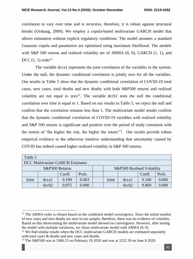
The variable dcca1 represents the joint correlation of the variables in the system.
Under the null, the dynamic conditional correlation is jointly zero for all the variables.
Our results in Table 5 show that the dynamic conditional correlation of COVID-19 total
cases, new cases, total deaths and new deaths with both S&P500 returns and realized
volatility are not equal to zero12. The variable dccb1 tests the null the conditional
correlation over time is equal to 1. Based on our results in Table 5, we reject the null and
confirm that the correlation remains less than 1. The multivariate model results confirm
that the dynamic conditional correlation of COVID-19 variables with realized volatility
and S&P 500 returns is significant and positive over the period of study consistent with
the notion of ‘the higher the risk, the higher the return’13. Our results provide robust
empirical evidence to the otherwise intuitive understanding that uncertainty caused by
COVID has indeed caused higher realized volatility in S&P 500 returns.
11 The ARMA order is chosen based on the combined model convergence. Since the initial number
of new cases and new deaths are zero in our sample, therefore, there was no evidence of volatility.
Based on this shortcoming the multivariate model showed no convergence. However, after testing
the model with multiple variations, we chose multivariate model with ARMA (0, 0) 12 We find similar results when the DCC multivariate GARCH models are estimated separately
with total cases & deaths and new cases and deaths. 13 The S&P500 was at 3386.15 on February 19 2020 and was at 3232.39 on June 8 2020.
Table 5
DCC Multivariate GARCH Estimates
S&P500 Returns
S&P500 Realised Volatility
Coeff. Prob.
Coeff. Prob.
Joint dcca1 0.109 0.063
Joint dcca1 0.100 0.000
dccb2 0.875 0.000
dccb2 0.869 0.000

NICE Research Journal, Vol.13 No.4 (2020): October-December ISSN: 2219-4282
93
4. CONCLUSION
In this paper, we analyse the patterns and trends in the intraday stock returns and
volatility in the US equity market amid the global COVID-19 pandemic. We use the
intraday 10-minute S&P500 index values as a proxy for stock prices in the US equity
market. Our descriptive analysis reveals that both returns and volatility exhibit different
patterns over the sample period in line and coinciding with the COVID-19 pandemic.
Average returns are negative (positive) and volatility is rising (falling) from January to
March 2020 (March to May 2020). Intraday day patterns in returns and volatility suggest
that the returns are mostly negatively and highly volatile in the last trading sessions
relative to earlier sessions in the day.
The findings from our univariate GARCH analysis and Nyblom parameters
stability test suggest structural break(s) in data in March 2020 after the first trading halt
took place on 9th March 2020. We find that different univariate GARCH specification
fits in each case for before and after the trading halt trading periods. Duly we employ
dynamic conditional correlation (DCC) multivariate GARCH to assess the relationship of
stock returns and volatility with the number of total and new cases as well as total deaths
and new deaths. Our empirical results confirm that COVID-19 cases and deaths (total and
new) have a statistically significant dynamic conditional correlation with stock returns
and volatility. Over time, we observe that the market has recovered from the panic in
March 2020 and a strategy of standing still and doing nothing would have enabled
investors to save on trading costs and taxes.
REFERENCES
Akhtaruzzaman, M., Boubaker, S. and Sensoy, A. (2020). Financial contagion during COVID–19 crisis. Finance Research Letters,
doi: https://doi.org/10.1016/j.frl.2020.101604 Baig, A., Butt, H., Haroon, O. and Rizvi, S.A.R. (2020). Deaths, Panic, Lockdowns and
US Equity Markets: The Case of COVID-19 Pandemic. Available at: https://papers.ssrn.com/sol3/papers.cfm?abstract_id=3584947
Baker, S.R., Bloom, N., Davis, S.J., Kost, K.J., Sammon, M.C. and Viratyosin, T. (2020). The unprecedented stock market impact of COVID-19. Becker Friedman Institute, University of Chicago. Available at: https://bfi.uchicago.edu/wp-content/uploads/BFI_White-Paper_Davis_3.2020.pdf
Chance, D.M. and Brooks, R., 2015. Introduction to derivatives and risk management.

NICE Research Journal, Vol.13 No.4 (2020): October-December ISSN: 2219-4282
94
Cengage Learning. Engle, R. (2002). Dynamic conditional correlation: A simple class of multivariate
generalized autoregressive conditional heteroskedasticity models. Journal of Business & Economic Statistics, 20(3), pp. 339-350.
doi: https://doi.org/10.1198/073500102288618487 Haroon, O. and Rizvi, S.A.R., 2020. COVID-19: Media coverage and financial markets
behavior—A sectoral inquiry. Journal of Behavioral and Experimental Finance, doi: https://doi.org/10.1016/j.jbef.2020.100343
Ibikunle, G. and Rzayev, K. (2020). Volatility, dark trading and market quality: evidence from the 2020 COVID-19 pandemic-driven market volatility. SRC Discussion Paper No. 95, London School of Economics and Political Science. Available at: https://papers.ssrn.com/sol3/papers.cfm?abstract_id=3586410
Mirza, N., Naqvi, B., Rahat, B. and Rizvi, S.K.A. (2020). Price reaction, volatility timing and funds’ performance during Covid-19. Finance Research Letters, doi: https://doi.org/10.1016/j.frl.2020.101657
Onali, E. (2020). Covid-19 and stock market volatility. University of Exeter Business School.Availableat:https://papers.ssrn.com/sol3/papers.cfm?abstract_id=3571453
Orskaug, E. (2009). Multivariate DCC-G model:-with various error distributions. Master's Thesis, Department of Mathematical Science, Norwegian University of Science and Technology. Available at: https://ntnuopen.ntnu.no/ntnu-xmlui/handle/11250/259296
Papadamou, S., Fassas, A., Kenourgios, D. and Dimitriou, D. (2020). Direct and indirect effects of COVID-19 pandemic on implied stock market volatility: evidence from panel data analysis. MPRA Paper No. 100020. Available at: https://mpra.ub.uni-muenchen.de/100020/
Siegel, L. (2020). The novelty of the coronavirus: what it means for markets. CFA Institute. Available at: https://blogs.cfainstitute.org/investor/2020/03/18/the-novelty-of-the-coronavirus-what-it-means-for-markets/
Zhang, D., Hu, M. and Ji, Q. (2020). Financial markets under the global pandemic of COVID-19.FinanceResearchLetters. doi: https://doi.org/10.1016/j.frl.2020.101528


