Graduate Theses, Dissertations, and Problem Reports
2019
Fundamental Mechanism of Time Dependent Failure in Shale Fundamental Mechanism of Time Dependent Failure in Shale
Neel Gupta [email protected]
Follow this and additional works at: https://researchrepository.wvu.edu/etd
Part of the Mining Engineering Commons
Recommended Citation Recommended Citation Gupta, Neel, "Fundamental Mechanism of Time Dependent Failure in Shale" (2019). Graduate Theses, Dissertations, and Problem Reports. 7445. https://researchrepository.wvu.edu/etd/7445
This Dissertation is protected by copyright and/or related rights. It has been brought to you by the The Research Repository @ WVU with permission from the rights-holder(s). You are free to use this Dissertation in any way that is permitted by the copyright and related rights legislation that applies to your use. For other uses you must obtain permission from the rights-holder(s) directly, unless additional rights are indicated by a Creative Commons license in the record and/ or on the work itself. This Dissertation has been accepted for inclusion in WVU Graduate Theses, Dissertations, and Problem Reports collection by an authorized administrator of The Research Repository @ WVU. For more information, please contact [email protected].

Fundamental Mechanism of Time-Dependent Failure in Shale
Neel Gupta
Dissertation submitted to the
Benjamin M. Statler College of Engineering and Mineral Resources
at West Virginia University
In partial fulfillment of the requirements for the degree of
Doctor of Philosophy
in
Mining Engineering
Brijes Mishra, Ph.D., Chair
Keith A. Heasley, Ph.D.
Edward M. Sabolsky, Ph.D.
John Quaranta, Ph.D.
Gabriel S. Esterhuizen, Ph.D.
Morgantown, West Virginia
2019
Keywords: Shale, creep, X-ray computed tomography, microcracking, image processing
Copyright 2019 Neel Gupta

ABSTRACT
Fundamental Mechanism of Time Dependent Failure in Shale
Neel Gupta
In underground coal mines, mining activity disturbs the natural equilibrium state of in-situ
stresses. The induced and in-situ stresses deform the rockmass surrounding the mine openings.
Primary roof supports impede the deformation of the rockmass overlying the entries. However,
failure can occur in the bolted rockmass, causing fatalities and injuries. The rockmass failure is
erratic, and its occurrence often varies from a few days to months and years after the opening of
the entry. One of the often-neglected factors in this process is the effect of time on the stability of
mine openings, which can often be observed in the propagation of failure in the rockmass. Coal-
measure rocks have exhibited time-dependent strength reduction in laboratory creep tests.
However, the exact mechanism responsible for this time-dependent reduction in strength is not
clear. Therefore, this thesis investigated the fundamental reason for macroscopic creep
deformation in shale through microscopic visualization using an X-ray computed tomography
(CT) technique. An approach was formulated based on the following experiments.
• Conduct compressive strength tests and X-ray powdered diffraction (XRD) analysis on
core specimens
• Perform triaxial creep tests at different triaxial stress states
• Determine the geometry of the microcracks using X-ray CT image processing
• Perform triaxial creep and recovery test with X-ray CT scan of shale specimens
The mineralogical analysis, using XRD, showed that the shale contained calcite, as well as a
minor percentage of quartz, feldspar, and illite. The uniaxial and triaxial compressive strength tests
showed brittle failure, with a high modulus of stiffness and a low Poisson’s ratio in the elastic
region. The creep behavior of shale was analyzed under constant triaxial stress. As shale is an
anisotropic rock, specimens were tested with both parallel and perpendicular bedding orientations
to the major principal stress. The triaxial experiments showed that both types of specimens
experienced creep failure; however, the creep deformation was unpredictable. The time to reach
creep failure did not show any correlation with the level of applied stress. The results of secondary
creep strain rate did not follow Norton’s creep law; the degree of determination (R2) between the
logarithm of secondary creep strain rate and logarithm of applied differential stress was
significantly small. In addition, the nature of creep deformation in brittle shale was different from
other brittle rocks, such as quartz and granite. In both parallel and perpendicular-bedded shale
specimens, the increase in confining pressure changed the inelastic volumetric strain, at the onset
of the tertiary creep stage, from dilation to the compression. The results of creep experiments
proved that shale exhibited creep deformation; however, its nature did not follow the established
empirical creep law.
The X-ray CT technique enabled the microscopic visualization of shale to a pixel resolution of
29.9 microns. However, limited research is available on the procedure for X-ray CT image
processing. Therefore, a “standard” procedure was developed to analyze the geometry of
microcracks in X-ray CT images using an open-source image analysis software, called FIJI. The

user-defined macros in FIJI efficiently processed the images and determined the geometry of
microcracks, such as volume, aperture, and area of the plane of the microcracks. Further, triaxial
creep and recovery tests were conducted on shale specimens and changes in the geometry of
microcracks was visualized between the pre- to post-test states using X-ray CT equipment. The
laboratory creep and recovery tests showed that the time-dependent strain in shale was a
combination of visco-elastic and visco-plastic strain. The X-ray CT scan in the pre-test state
showed that shale specimens contained a significant volume of pre-existing microcracks, which
varied among specimens. The X-ray CT scan in the post-test state showed that the volume of
microcracks after creep and recovery test depends on the time under constant stress, as well as the
volume of pre-existing microcracks. The growth of both plane and aperture of microcracks caused
the inelastic strain in the axial and radial directions, respectively. The orientation of bedding planes
influenced the nature of the change in the geometry of microcracks. Therefore, it was concluded
that the microcracking was the fundamental reason for creep deformation in shale.

iv
ACKNOWLEDGEMENTS
I would like to extend my sincere thanks to my thesis advisor and mentor Dr. Brijes Mishra for
his continued support, guidance, patience and encouragement throughout my doctoral research.
His valuable insights and suggestions will always be cherished. It was a wonderful opportunity to
perform research under his supervision.
I would also like to thank the members of my thesis committee, Drs. Keith A. Heasley, Edward
M. Sabolsky, John Quaranta and G.S. Esterhuizen, for their valuable comments and suggestions.
I would also like to thank the National Institute of Occupational Safety and Health (NIOSH)
for providing the necessary funding for this research. I would also like to thank the Office of
Graduate Education and Life (OGEL) of WVU which in part supported this research by providing
an Outstanding Merit Fellowship for Continuing Doctoral Student. I would also like to thank Dr.
Dustin Crandall, Dr. Sarah Brown, Johnathan E. Moore and Bryan Tennant at the National Energy
Technology Laboratory (NETL) in Morgantown, West Virginia for support of the X-ray CT scans
of the shale specimens.
A sincere thanks to the Animal Models and Imaging Facility (AMIF) of WVU, especially Dr.
Karen Martin and Sarah McLaughin for provide the access to Bruker CTAn software for image
processing. I would also like to thank Dr. Qiang Wang from the Material Characterization
Facilities for training me on X-ray diffraction (XRD) instruments. I am also thankful to Dr.
Qingqing Huang for letting me use the WVU mineral processing laboratory for preparing specimen
for the powdered XRD analysis.
I would like to express my appreciation to Karen Centofanti and Genette Chapman for their
help and contribution in purchasing numerous supplies for experiments and expediting the official
departmental work. I would also like to thank Yuting Xue, Prasoon Garg, Danqing Gao, Debashis
Das, Bonaventura Alves, Grant Speer, Chris Vaas and Qingwen Shi for being amazing colleagues
and helping me in my research.
Lastly, I would like to thank my family for their continued encouragement and support during
my study. Finally, I thank God for carrying me through all the joys and sorrows during my stay at
WVU and making me a better person through each passing day.
v
TABLE OF CONTENTS Chapter 1 Introduction ............................................................................................................................... 1
1.1 Statement of the Problem .................................................................................................................... 9
1.2 Objective ........................................................................................................................................... 10
Chapter 2 Literature review .................................................................................................................... 12
2.1 Creep study in coal-measure shale from underground coal mines.................................................... 13
2.2 Creep study in shale from oil wells, tunnels, and nuclear waste repository ..................................... 20
2.3 Application of rheological models to simulate creep deformation ................................................... 23
2.4 Creep in Ductile Rock Salt ............................................................................................................... 29
2.5 Creep in Brittle Quartz ...................................................................................................................... 34
2.6 Summary of the literature review...................................................................................................... 40
Chapter 3 Characterization of Mineralogy and Compressive Strength of Shale ............................... 42
3.1 Uniaxial and Triaxial Compressive Strength Tests ........................................................................... 43
3.2 Mineralogy of Marcellus shale through X-ray powdered diffraction ............................................... 50
3.3 Summary ........................................................................................................................................... 56
Chapter 4 Triaxial Creep Test on Bedded Marcellus Shale ................................................................. 57
4.1 Experimental procedure of triaxial creep experiments ..................................................................... 57
4.2 Results of triaxial creep experiments ................................................................................................ 59
4.3 Summary ........................................................................................................................................... 72
Chapter 5 Procedure of X-ray Computed Tomography (CT) Scanning and Image Processing to
Analyze Geometry of Microcracks .......................................................................................................... 73
5.1 Introduction of X-ray CT Equipment ................................................................................................ 73
5.2 X-ray computed tomography (CT) image processing ....................................................................... 76
5.2.1 Image processing using Global Thresholding technique ........................................................... 77
5.2.2 Image processing using Adaptive (Local) Thresholding technique ........................................... 78
5.2.3 Image processing using Adaptive Thresholding technique on pre-processed X-ray CT image 79
5.2.4 Image processing using new proposed workflow in FIJI ........................................................... 81
5.2.5 Automation of image processing in FIJI .................................................................................... 86
5.3 Geometry of microcracks from binary X-ray CT images ................................................................. 87
5.3.1 Two-dimensional (2-D) geometry of microcracks ..................................................................... 88
5.3.2 Three-dimensional (3-D) geometry of microcracks ................................................................... 95
5.4 Summary ......................................................................................................................................... 100

vi
Chapter 6 Assessment of the Geometry of Microcracks during Triaxial Creep and Recovery Tests
using the X-ray CT Scan Technique ..................................................................................................... 102
6.1 Procedure for the triaxial creep and recovery test with X-ray CT scan .......................................... 102
6.1.1 Type 1 triaxial creep and recovery test with X-ray CT scan .................................................... 103
6.1.2 Type 2 Triaxial Creep and Recovery Test with X-ray CT Scan .............................................. 104
6.2 Time-dependent strain in the rock subjected to constant stress state .............................................. 106
6.3 Results of the triaxial creep and recovery test with X-ray CT scan ................................................ 108
6.3.1 Results of Type 1 triaxial creep and recovery test on bedded Marcellus shale........................ 109
6.3.2 Results of Type 2 triaxial creep and recovery test on bedded Marcellus shale........................ 114
6.3.3 Change in geometry of microcracks during Type 1 triaxial creep and recovery test ............... 120
6.3.4 Change in geometry of microcracks during Type 2 triaxial creep and recovery test ............... 131
6.4 Comparison between permanent strain and stress-induced change in geometry of microcracks in
bedded Marcellus shale ......................................................................................................................... 140
6.5 Summary ......................................................................................................................................... 143
Chapter 7 Discussions and Conclusions ................................................................................................ 144
Chapter 8 Future Work .......................................................................................................................... 147
References ................................................................................................................................................ 149
Appendix .................................................................................................................................................. 165
A. Macro to enhance contrast and segment microcracks – Case IV ..................................................... 165
B Macro for calculating area, weighted-mean aperture, and length of microcracks of an individual 2-D
image in FIJI ......................................................................................................................................... 166
C. Script to summarize the 2-D geometry of microcracks in MATLAB .............................................. 167
D. Comparison between Measured and Calculated Volume of 3-D Rectangular Microcrack ............. 168

vii
LIST OF FIGURES
Figure 1.1 Generalized stratigraphic column of the Upper Pennsylvanian Monongahela Group showing
major coal beds (Tewalt et al., 2001) ............................................................................................................ 2
Figure 1.2 Generalized cross section of the Pittsburgh coal bed trending from Harrison County, WV to
Allegheny County, PA (Tewalt et al., 2001) ................................................................................................. 3
Figure 1.3 Historical overview of groundfall fatalities from 1906-2018 ...................................................... 4
Figure 1.4 Roof deterioration in moisture-sensitive shale roof in the Herrin #6 seam of Illinois coalmine
(Molinda and Klemetti, 2008) ....................................................................................................................... 7
Figure 1.5 Heavily loaded roof screen supporting the weak shale roof in Herrin #6 seam of Illinois
coalmine (Molinda and Klemetti, 2008) ....................................................................................................... 8
Figure 1.6 Cutters in the immediate roof on the face of a longwall gateroad development entry immediate
after cutting (Ray, 2009) ............................................................................................................................... 9
Figure 2.1 A classic trimodal creep curve (Heap, 2009)............................................................................. 12
Figure 2.2 Relation between Time Effect and Load (Phillips, 1931) ......................................................... 13
Figure 2.3 Creep of Conchas shale loaded to 10.4 kg/cm2 at room temperature (Griggs, 1939) ................ 14
Figure 2.4 Creep of the shale (dry) under compressive force of 400, 500, 600, and 960 kg/cm2 (Nishihara,
1952) ........................................................................................................................................................... 15
Figure 2.5 Creep of the sandy shale (wet) under compressive force of 80, 160, 240, and 320 kg/cm2
(Nishihara, 1952) ........................................................................................................................................ 16
Figure 2.6 Overall time-strain curve for a specimen of calcareous siltstone from Wolstanton Colliery
(Price, 1964) ................................................................................................................................................ 17
Figure 2.7 Time-strain data for specimen No. 3 of nodular muddy limestone from Warsop Colliery (Price,
1964) ........................................................................................................................................................... 17
Figure 2.8 Axial strain-time curve for Appin Colliery shale (Singh, 1975) ............................................... 19
Figure 2.9 Experimental observation on the relation between confining stress and failure modes for soft
rock under creep deformation (Liu and Zhou, 2000) .................................................................................. 21
Figure 2.10 Basic Rheological elements: (a) Hookean element; (b) Newtonian element; (c) St. Venant
element ........................................................................................................................................................ 24
Figure 2.11 Maxwell Model: (a) Schematic Diagram; (b) Strain-Time Curve ........................................... 25
Figure 2.12 Kelvin Voight Model: (a) Schematic Diagram; (b) Strain-Time Curve .................................. 25
Figure 2.13 Poynting Thomsen Model: (a) Schematic Diagram; (b) Strain-Time Curve ........................... 26
Figure 2.14 Burger Model: (a) Schematic Diagram; (b) Strain-Time Curve .............................................. 26
Figure 2.15 Bingham Model: (a) Schematic Diagram; (b) Strain-Time Curve .......................................... 27
Figure 2.16 Series Combination of Burger and Bingham Model: (a) Schematic Diagram; (b) Strain-Time
Curve ........................................................................................................................................................... 27
Figure 2.17 Schematic representation of (a) edge and (b) screw dislocations in a cubic crystalline
material, where filled circles denote the lattice points of a crystal, b is a Burgers vector, hatched area and
dashed line show the slip plane and dislocation line, respectively (Dontsova, 2013) ................................ 32
Figure 2.18 Evolution of shear stress (τ) and dislocation density (ρ) in slip system versus the total shear
strain (γp) in the Dislocation Dynamics Simulation of tensile deformation in copper crystals (Devincre et
al., 2008) ..................................................................................................................................................... 34
Figure 2.19 Schematic representation of the experimental methodology of creep experiments on granite
(Kranz, 1979) .............................................................................................................................................. 39

viii
Figure 2.20 Separation of two-feldspar grain through boundary in the vertical direction because of loading
(Kranz, 1979) .............................................................................................................................................. 39
Figure 3.1 Index map of stratigraphic cross-sections and the Devonian Outcrop belt in the Appalachian
Basin (Roen, 1984) ..................................................................................................................................... 42
Figure 3.2 Servo-controlled MTS-810 testing equipment and its components: (1) Load frame; (2)
Hydraulic actuator; (3) Strain gauge control panel; (4) MTS data acquisition system; (5) Computer; (6)
Upper steel platen; (7) Lower steel platen (Das, 2018) .............................................................................. 43
Figure 3.3 Shale specimen in the load frame of the MTS-810 mounted with the radial extensometer ...... 44
Figure 3.4 Axial Splitting of Marcellus shale specimen under unconfined compressive stress (a) parallel-
bedded, (b) perpendicular-bedded............................................................................................................... 45
Figure 3.5 Laboratory setup of GCTS RTX-1500 (Mishra and Verma, 2015) ........................................... 46
Figure 3.6 Comparison of average axial strength at four different confining conditions in parallel- and
perpendicular- bedded shale specimens ...................................................................................................... 48
Figure 3.7 Variation of axial strength with the orientation of discontinuity (Hoek & Bown, 1980) .......... 48
Figure 3.8 Axial stress-strain curve in Triaxial Strength Test: (a) Parallel Specimen; (b) Perpendicular
Specimen ..................................................................................................................................................... 49
Figure 3.9 Failure of (a) Parallel-bedded, (b) Perpendicular-bedded shale specimen along shear plane
under triaxial compressive stress ................................................................................................................ 50
Figure 3.10 PANalytical X'Pert Pro X-ray Diffractometer (Das, 2018) ..................................................... 51
Figure 3.11 Step-wise reduction of solid rock specimen into the powder sized less than 45 microns; (a)
Jaw crusher; (b) Ball mill; (c) RO-TAP sieve shaker; (d) Powder form of shale specimen ....................... 53
Figure 3.12 (a) Different parts of the specimen preparation kit; (b) specimen holder filled with powdered
specimen ..................................................................................................................................................... 54
Figure 3.13 X-ray Diffractogram of Marcellus shale specimen ................................................................. 55
Figure 4.1 Stress-strain curve for Darley Dale sandstone (Heap, 2009) ..................................................... 58
Figure 4.2 The comparison between the time to reach the onset of tertiary creep stage and level of
differential stress in parallel-bedded specimens ......................................................................................... 62
Figure 4.3 The comparison between the time to reach the onset of tertiary creep stage and level of
differential stress in perpendicular-bedded specimens ............................................................................... 62
Figure 4.4 Logarithm of the failure time in seconds versus stress difference in kilobars at confining
pressure of 1 bar, 530 bars, 1000 bars, and 1980 bars(Kranz, 1980). Best fit, least squares regression lines
and R2 are shown ........................................................................................................................................ 63
Figure 4.5 Creep strain versus time curve for bedded shale specimens ...................................................... 68
Figure 4.6 Fitting of linear trend between log (axial creep rate) and log (differential stress) for bedded
shale specimens ........................................................................................................................................... 69
Figure 4.7 Fitting of linear trend between log (radial creep rate) and log (differential stress) for bedded
shale specimens ........................................................................................................................................... 69
Figure 4.8 Dilatant volumetric strain at the onset of the tertiary creep stage as a function of confining
pressure. Open symbols represent constant-rate fracture tests; closed symbols represent creep tests. Error
bars are standard deviation and compression is negative (Kranz, 1980) .................................................... 70
Figure 4.9 The relationship between inelastic volumetric strain and confining pressure in constant strain
rate and creep tests for: (a) parallel-bedded specimens; (b) perpendicular-bedded specimens .................. 71
Figure 5.1 X-ray CT image with crack and intact rock ............................................................................... 74
Figure 5.2 NorthStar Imaging M-5000 Industrial CT scanner: (a) X-ray detector with vertical sandstone
core, (b) X-ray source with vertical sandstone core (Rodriguez et al., 2014) ............................................. 75
ix
Figure 5.3 (a) Two-dimensional grayscale image from X-ray CT scan of shale specimen; (b) Three-
dimensional image reconstructed from the stack of two-dimensional images ............................................ 76
Figure 5.4 (a) Original grayscale X-ray CT image; (b) Results of Global Thresholding through different
algorithms ................................................................................................................................................... 77
Figure 5.5 (a) Original grayscale X-ray CT image; (b) Results of Adaptive Thresholding through different
algorithms ................................................................................................................................................... 79
Figure 5.6 Comparison of the GSV across the Image Width: (a) Original X-ray CT Image; (b) Beam-
Hardening corrected X-ray CT Image ........................................................................................................ 80
Figure 5.7 (a) B-Hc X-ray CT image; (b) Results of Adaptive Thresholding through different algorithms
.................................................................................................................................................................... 81
Figure 5.8 Manual Adjustment of Brightness/Contrast of original X-ray CT Image ................................. 82
Figure 5.9 Comparison of GSV along the purple line among similar X-ray CT images at different contrast
levels. (a) Original X-ray CT image; (b) Manually Adjusted Brightness and Contrast in Original X-ray
CT image; (c) Local contrast enhancement in Original X-ray CT image ................................................... 83
Figure 5.10 Process of Trainable Weka Segmentation: (a) Tracing of Microcracks and Intact Rock in
Contrast Enhanced X-ray CT Image; (b) Colored Segmentation of X-ray CT Image; (c) Binary-
Microcracks Segmented X-ray CT Image .................................................................................................. 85
Figure 5.11 Workflow of new proposed image processing technique ........................................................ 86
Figure 5.12 (a) Montage of 2-D binary X-ray CT images spaced at 2.97 millimeters; (b) 3-D microcracks
reconstructed from 2-D binary images spaced at 29.7 microns .................................................................. 87
Figure 5.13 Different component of 2-D microcrack in binary X-ray CT image ....................................... 88
Figure 5.14 Results of the function Analyze Particles in FIJI .................................................................... 89
Figure 5.15 2-D Aperture of Microcracks using Thickness (BoneJ) in FIJI............................................... 90
Figure 5.16 2-D Length of Microcracks using Analyze Skeleton in FIJI ................................................... 91
Figure 5.17 (a) 3-D distribution of microcracks reconstructed from 2-D binary X-CT images; (b) Scatter
plot between individual slice position and cumulative 2-D area of microcracks; (c) Scatter plot between
individual slice position and weighted-mean 2-D aperture of microcracks; (d) Scatter plot between
individual slice position and cumulative 2-D length of microcracks .......................................................... 93
Figure 5.18 Visual comparison of the microcracks in the 2-D binary image at the individual slice position
of: (a) 925; (b) 926 ...................................................................................................................................... 94
Figure 5.19 (a) Sequential stack of 2-D binary X-ray CT images; (b) Results of the plugin Volume
Fraction in FIJI ............................................................................................................................................ 95
Figure 5.20 (a) Three-dimensional view of color contour of aperture of microcracks; (b) Three-
dimensional weighted-mean aperture of microcracks using Thickness in FIJI .......................................... 96
Figure 5.21 Distribution of local 3-D aperture of microcracks in Figure 5.12(b) using FIJI...................... 97
Figure 5.22 Pictorial representation of 3-D microcrack: (a) regenerated from 2-D binary images; (b)
regenerated from 2-D skeletonized binary images...................................................................................... 98
Figure 5.23 3-D distribution of microcracks, where different colors represent different 3-D apertures of
the microcracks ......................................................................................................................................... 100
Figure 6.1 Experimental procedure for Type 1 triaxial creep and recovery test with X-ray CT scan ...... 103
Figure 6.2 Experimental procedure for Type 2 triaxial creep and recovery test with X-ray CT scan ...... 105
Figure 6.3 Time dependent creep deformation of concrete (Mehta & Monteiro, 2006) ........................... 107
Figure 6.4 Decomposition of time-dependent strain in HMA from creep and recovery testing (Kim et al.,
2009) ......................................................................................................................................................... 107

x
Figure 6.5 Disintegration of differential stress versus time curve into different regions based on the nature
of differential stress ................................................................................................................................... 108
Figure 6.6 Axial stress versus strain curves for Type 1 triaxial creep and recovery tests ........................ 110
Figure 6.7 Strain versus time curve for Type 1 triaxial creep and recovery test ...................................... 111
Figure 6.8 The comparison between creep strain versus time under constant stress for parallel- (PL) and
perpendicular- (PD) bedded shale specimens ........................................................................................... 114
Figure 6.9 Axial Stress versus Strain curve for Type 2 Triaxial Creep and Recovery Test ..................... 116
Figure 6.10 Strain versus Time curve for Type 2 Triaxial Creep and Recovery Test .............................. 116
Figure 6.11 The comparison of axial creep strain with the level of differential stress in Type 2 creep and
recovery experiment .................................................................................................................................. 120
Figure 6.12 Comparison between stress-induced change in geometry of microcracks and time of constant
stress state for: (a) Perpendicular-bedded specimens; (b) Parallel-bedded specimens ............................. 122
Figure 6.13 The graph between cumulative 2-D area of microcracks and individual slice position in pre-
and post-stress state for Type 1 triaxial creep and recovery test ............................................................... 126
Figure 6.14 Vertical projection of 2-D microcracks in pre- and post-stress state in Type 1 triaxial creep
and recovery test ....................................................................................................................................... 128
Figure 6.15 Three-dimensional comparison of microcracks in pre-and post-stress state in perpendicular
specimens of Type 1 triaxial creep and recovery test ............................................................................... 129
Figure 6.16 Three-dimensional comparison of microcracks in pre-and post-stress state in parallel
specimens of Type 1 triaxial creep and recovery test ............................................................................... 130
Figure 6.17 The comparison between stress induced change in area and volume of microcracks with level
of differential stress for: (a) Perpendicular-bedded specimens; (b) Parallel-bedded specimens. ............. 133
Figure 6.18 The graph between cumulative 2-D area of microcracks and individual slice position at three
different time steps in Type 2 triaxial creep and recovery test ................................................................. 135
Figure 6.19 Comparison of vertical projection of 2-D microcracks at three different time steps in Type 2
triaxial creep and recovery test ................................................................................................................. 137
Figure 6.20 Three-dimensional distribution of microcracks in pre-stress, post-cycle 1, and post-cycle 2 of
Type 2 triaxial creep and recovery test ..................................................................................................... 139
Figure 6.21 The graph between permanent axial strain and change in area of plane of microcracks in
perpendicular-bedded specimens .............................................................................................................. 141
Figure 6.22 The graph between: (a) Permanent axial strain and change in area of plane of microcracks; (b)
Permanent radial strain and change in 3-D weighted mean aperture of parallel-bedded specimens ........ 142
Figure 8.1 Microcrack propagation in silica under the influence of water (A) atomistic view of a crack tip
in silica glass; (B) adsorption of water molecule at stressed Si-O-Si linkage (Rodrigues et al., 2017) ... 147
Figure D.1 Comparison between measured and calculated volume of microcracks…………………….169

xi
LIST OF TABLES
Table 1.1 MSHA reported roof fall accidents in underground coal mines ................................................... 5
Table 3.1 Results of unconfined compression strength test ........................................................................ 45
Table 3.2 Results of triaxial compressive strength tests ............................................................................. 47
Table 3.3 Mineralogy of Marcellus shale ................................................................................................... 55
Table 4.1 Details of triaxial creep experiments on bedded Marcellus shale ............................................... 59
Table 4.2 Results of rate of secondary creep strain and inelastic volumetric strain during triaxial creep test
.................................................................................................................................................................... 64
Table 5.1 Comparisons of average value of 2-D geometry of microcracks determined through FIJI and
Bruker CTAn .............................................................................................................................................. 92
Table 5.2 Results of 3-D geometry of microcracks using FIJI and Bruker CTAn software ....................... 99
Table 6.1 Results of the Type 1 experiment on bedded Marcellus shale .................................................. 112
Table 6.2 Different types of strain in shale specimen during Type 1 triaxial creep and recovery test ..... 113
Table 6.3 Results of Type 2 triaxial creep and recovery test on bedded Marcellus Shale ........................ 117
Table 6.4 Comparison of elastic and plastic components of axial and radial strain between stress cycle 1
and cycle 2 ................................................................................................................................................ 118
Table 6.5 Different types of strain in shale specimen during Type 2 triaxial creep and recovery test ..... 119
Table 6.6 Comparison of 2-D area and 3-D volume of microcracks tested in Type 1 triaxial experiment
.................................................................................................................................................................. 121
Table 6.7 Comparison of 2-D and 3-D geometrical parameters to analyze the mode of change in area and
volume of microcracks in Type 1 triaxial experiment .............................................................................. 124
Table 6.8 Comparison of 2-D area and 3-D volume of microcracks in Type 2 triaxial creep and recovery
test ............................................................................................................................................................. 131
Table 6.9 Comparison of weighted-mean aperture and length of microcracks in 2-D at three different time
steps .......................................................................................................................................................... 134
Table 6.10 Comparison of weighted-mean aperture and area of plane of microcracks in 3-D at three
different time steps .................................................................................................................................... 134
Table D.1 Measured and Calculated 3-D geometrical parameters of microcracks………………………168

1
Chapter 1 Introduction
Room-and-pillar and longwall are two of the most popular underground coal extraction methods
in the United States. Both methods develop rooms known as entries and leave large blocks of coal
known as pillars to support the overburden strata. In room-and-pillar mining, the entry width varies
between 16 to 20 feet. Similarly, longwall mining uses a chain pillar system to support the
overlying rock above the headgate and tailgate entries, whose widths vary between 16 to 20 feet.
After underground excavation, the overburden strata settle under the overlying load and the
redistributed stresses in the roof can cause significant deformation (Medhurst et al., 2014). In the
Appalachian Basin, the extensive mining of the Pittsburgh coal seam covers an area extending
over 11,000 sq. miles through 53 counties in Pennsylvania, West Virginia, Ohio, and Maryland
(Tewalt et al., 2001). Figure 1.1 displays the generalized stratigraphic column of the Upper
Pennsylvanian Monongahela Group; it shows that the Pittsburgh coal bed, which lies at the base
of the Monongahela group, is directly overlaid by either: 1) shale and siltstone, 2) coal, or 3) coal
and shale; and often has shale as the floor underlying the coal. Figure 1.2 shows an example of a
generalized cross section of the Pittsburgh coal bed trending from Harrison County, West Virginia
(WV), to Allegheny County, Pennsylvania (PA). In this region, shale, siltstone, and claystone
(shown in green in Figure 1.2) and coal or coal and shale (shown in gray in Figure 1.2) are the
major rock types that lie immediately above the coal seam. In addition, fireclay (shown in gold in
Figure 1.2) is the major rock type present under the coal seam. The example of Pittsburgh coal
seam in the Appalachian Basin signifies that the shale is a commonly present immediate roof in
underground coal mines.

2
Figure 1.1 Generalized stratigraphic column of the Upper Pennsylvanian Monongahela Group showing major coal
beds (Tewalt et al., 2001)

3
Figure 1.2 Generalized cross section of the Pittsburgh coal bed trending from Harrison County, WV to Allegheny
County, PA (Tewalt et al., 2001)
Shale is a sedimentary rock in the Earth’s crust (Krumbein and Sloss, 1963) and the most
common roof-rock above coal seams (Stevenson, 1913). With numerous thin bedding planes, it is
anisotropic in mechanical strength. The rock is stronger in the direction perpendicular to the
bedding planes than in the parallel direction (Molinda and Mark, 1996). It is also often moisture
sensitive, and previous research shows moisture induced weakening in the rockmass (Molinda et
al., 2006). It is the weakest unit of coal measure rocks in underground coal mines with the average
Coal Mine Roof Rating (CMRR) of 35 (Molinda, 2003; Murphy, 2016). Pappas and Mark (2010)
showed that a disproportionately large amount of roof falls occur in mines with a weak roof of
CMRR <=40. Therefore, the exposure of shale rock as immediate coal roof to the mine personnel
can pose serious ground control or roof fall problems in underground coal mines.
According to the National Institute of Occupational Safety and Health (NIOSH), roof fall
caused 33.3% of fatalities in underground coal mines (Mining Facts - 2015). Based on the Mine

4
Safety and Health Administration (MSHA) database studied by Pappas and Mark (2012), Figure
1.3 shows the frequency of roof and rib fall fatalities from the year 1906 to 2018. This figure shows
that in the early 1930’s, roof and rib fall fatalities occurred around 1,000 times annually and have
decreased gradually over time. Researchers assumed that the reasons for the reduction in roof fall
fatalities were: mechanizations of mining methods, installation of mechanical and resin-grouted
roof bolts, application of automated temporary roof supports (ATRS), and canopies, and
mandatory ground control safety and training programs by MSHA (Pappas, 1987). Although
advanced engineering supports have reduced the number of roof falls, the incidents have not stop
completely. In 1998, roof and rib falls injured 850 workers and caused 26,000 days lost of work
(Pappas et al., 2000). Bajpayee et al. (2014) showed that the number of non-injury roof fall
incidents ranged between 979 and 1,363 for every year from 1999 through 2008. The major
contributing geologic factors toward roof falls were geologic defects in the roof-rock, moisture
degradation of shale, and cutter failure in laminated roof (Bajpayee et al., 2014). The small
frequency of fatalities in the histogram from the years 1995 to 2018 in Figure 1.3 also shows that
a few roof and rib fall fatalities continue in underground coal mines. This small, yet critical,
number of falls in permanently supported roof encourages the continued laboratory research into
ground control problems.
Figure 1.3 Historical overview of groundfall fatalities from 1906-2018
5
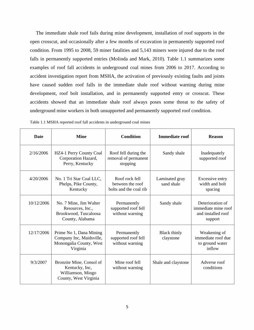
The immediate shale roof fails during mine development, installation of roof supports in the
open crosscut, and occasionally after a few months of excavation in permanently supported roof
condition. From 1995 to 2008, 59 miner fatalities and 5,143 miners were injured due to the roof
falls in permanently supported entries (Molinda and Mark, 2010). Table 1.1 summarizes some
examples of roof fall accidents in underground coal mines from 2006 to 2017. According to
accident investigation report from MSHA, the activation of previously existing faults and joints
have caused sudden roof falls in the immediate shale roof without warning during mine
development, roof bolt installation, and in permanently supported entry or crosscut. These
accidents showed that an immediate shale roof always poses some threat to the safety of
underground mine workers in both unsupported and permanently supported roof condition.
Table 1.1 MSHA reported roof fall accidents in underground coal mines
Date Mine Condition Immediate roof Reason
2/16/2006 HZ4-1 Perry County Coal
Corporation Hazard,
Perry, Kentucky
Roof fell during the
removal of permanent
stopping
Sandy shale Inadequately
supported roof
4/20/2006 No. 1 Tri Star Coal LLC,
Phelps, Pike County,
Kentucky
Roof rock fell
between the roof
bolts and the coal rib
Laminated gray
sand shale
Excessive entry
width and bolt
spacing
10/12/2006 No. 7 Mine, Jim Walter
Resources, Inc.,
Brookwood, Tuscaloosa
County, Alabama
Permanently
supported roof fell
without warning
Sandy shale Deterioration of
immediate mine roof
and installed roof
support
12/17/2006 Prime No 1, Dana Mining
Company Inc, Maidsville,
Monongalia County, West
Virginia
Permanently
supported roof fell
without warning
Black thinly
claystone
Weakening of
immediate roof due
to ground water
inflow
9/3/2007 Bronzite Mine, Consol of
Kentucky, Inc,
Williamson, Mingo
County, West Virginia
Mine roof fell
without warning
Shale and claystone Adverse roof
conditions

6
6/16/2008 Harmony Mine, UAE
Coalcorp Associates,
Mount Carmel,
Northumberland County,
Pennsylvania
Coal cutting from the
end of the pillar
during retreat mining
Very hard, dark
grey shale with
slickenside
Adverse roof
conditions
7/25/2008 Buchanan Mine #1,
Consolidation Coal
Company, Mavisdale,
Buchanan County,
Virginia
Mine roof fell during
marking roof bolt
between ATRS and
operator's canopy
Thinly bedded to
finely laminated
hard gray shale
Activation of
slickenside
formation in
unsupported area
4/28/2010 Dotiki Mine, Webster
County Coal, LLC, Nebo,
Hopkins County,
Kentucky
Draw rock fell in the
unbolted face of mine
entry
Black shale
overlain by gray
shale with pyrite
nodules
Activation of
slickenside
formation in
unsupported area
9/26/2012 Double Mountain Mine
Kopper Glo Mining, LLC,
Clairfield, Claiborne
County, Tennessee
Continuous miner
operator was inby of
permanently
supported roof
Medium hard, dark
gray, thin bedded
shale
Continuous mining
operator standing
under unsupported
roof
3/13/2013 Newton Energy, Inc.,
Peerless Rachel Mine,
Comfort, Boone County,
West Virginia
Roof rock fell
towards the roof
bolting machine
6.67 feet thick gray
shale
Miners exposed to
the unsupported roof
11/10/2014 Red Bone Mining
Company, Crawdad No. 1
Mine, Maidsville,
Monongalia County, West
Virginia
Roof rock fell
between the mine rib
and the canopy of a
roof bolting machine
Shale Failure in
identifying the roof
anomaly prior to
positioning of roof
bolting machines
2/20/2015 Heilwood mine, Rosebud
Mining Company, Inc.
Heilwood, Indiana
County, Pennsylvania
Roof rock fell
between last row of
permanent supports
and the ATRS
Gray shale bed Failure of mine
operator in
regulating the mine
operations in
inadequate
supported area
2/23/2017 Mine No. 5, C K Coal
Corporation, Delbarton,
Mingo County, West
Virginia
Inadequately
supported roof rock
fell, crushing the
miner against the
mine floor
Bed of shale rock
ranged between 4
inches to 2 feet in
thickness
Inadequate supports
to control the mine
roof

7
The moisture degradation of weak roof-rocks, such as mudstone or clay-enriched shale, was
one of the primary reasons of skin failure in underground coal mines. It refers to the failure of
small pieces or slabs of roof and rib (Bauer & Dolinar, 2000). Figure 1.4 shows the severely
deteriorated laminated shale roof near the intake shaft of the Herrin #6 seam in central Illinois
(Molinda and Klemetti, 2008). The roof consisted of weak shale from 0 to 6 feet thick, overlaid by
thick, weak gray shale. The exposure to moisture for four years deteriorated the roof and rib and
prevented access through the area. Screening the weak roof, spraying on sealants, and using fully
grouted roof bolts were possible engineering solutions to the degraded roof (Klemetti et al., 2009).
Figure 1.5 shows an example of screened roof that was 14 years old immediately adjacent to the
area shown in Figure 1.4. Molinda et al. (2006) found that mine entries with weak, moisture-
sensitive roofs were much more prone to deterioration due to the continuously changing
temperature and humidity inside an underground mine. Therefore, many researchers explained the
degradation phenomenon as time-dependent deterioration of moisture-sensitive shale rock
(Molinda and Klemetti, 2008; Klemetti et al., 2009).
Figure 1.4 Roof deterioration in moisture-sensitive shale roof in the Herrin #6 seam of Illinois coalmine (Molinda
and Klemetti, 2008)

8
Figure 1.5 Heavily loaded roof screen supporting the weak shale roof in Herrin #6 seam of Illinois coalmine
(Molinda and Klemetti, 2008)
Another important ground control problem is cutter failure in laminated roof rock. This failure
mechanism was one of the most visible ground control problems in underground mines operating
in the Pittsburgh coal seam (Hill, 1986). It is a compressional form of failure that initiates at the
corner of the mine entry and extends through the entire laminated roof span up to 18 feet (Mishra
and Verma, 2015). Figure 1.6 shows an example of cutter roof failure at the face of a longwall
gateroad (Ray, 2009). Su and Peng (1987) examined the fundamental causes of cutter roof failure
through field investigations, laboratory testing, underground instrumentation, and numerical
modelling. Their study found that high vertical stresses, excess horizontal stresses, and the relative
stiffness of coal and the immediate roof rock were some of the primary reasons for the formation
of cutter roof in West Virginia longwall coal mines. Other studies reported similar observations
through in-situ measurements and complex numerical models (Ahola et al., 1991; Gadde and Peng,
2005a). Proposed solutions to cutter failure included changes in pillar size, pillar softening, and
reorientation of mine entries to a direction 45° from either the maximum or the minimum principal
horizontal stress (Su and Peng, 1987). Gadde and Peng (2005b) proposed a strain-softening
numerical model to analyze cutter roof failure in weak roofs. Gao and Stead (2013) simulated
cutter failure due to the orientation of the maximum horizontal stress and the excavation direction
in three-dimensional distinct element code (3DEC) and three-dimensional particle flow code
(PFC3D). Since cutter-failure was not an instantaneous deformation (Ray, 2009) and numerical

9
simulation of cutter failure did not often include a time factor (Peng, 2015), the results of numerical
simulation did not always match the field observations and the exact understanding of the cutter
roof problem remains unresolved. The time-dependent nature of cutter roof indicated that time
should be a prominent factor in the assessment of the deformational behavior of shale roof.
Figure 1.6 Cutters in the immediate roof on the face of a longwall gateroad development entry immediate after
cutting (Ray, 2009)
1.1 Statement of the Problem
In underground coal mines, the excavation-induced stresses deform the surrounding rockmass.
The permanently supported or unsupported mine entries with shale in the immediate mine roof
undergo unexpected failure. Presence of stress and moisture induces time-dependent behavior in
shale. As failure of roof in the supported entries have often occurred, it is imperative to investigate
the fundamental reason of time-dependent (or creep) failure in shale. In the past, researchers have
used both numerical and empirical techniques to understand the time-dependent deformation in
shale. The laboratory experiments identified the vital parameters that affect the time-dependent
deformation of shale, and numerical or empirical models reproduced the time-dependent
deformational behavior. However, the experiments did not accurately describe the physical basis
for the time-dependent behavior (Senseny, 1983). One of the reasons for the shortcoming was
exclusion of the initial condition and nature of the rock that are subjected to constant load.

10
The physical basis for the time-dependent deformation in a rock is investigated through the
correlation of macroscopic permanent deformation with the microscopic changes in the rock under
constant stress state. Linear variable differential transformers (LVDTs), directly mounted on the
rock specimens accurately measure the macroscopic permanent deformation. In the past,
researchers used acoustic emission or scanning electron microscope (SEM) to analyze the
microscopic changes in the rock during creep experiments. However, these methods did not
consider the initial condition of the rock specimens, and only interpreted the test results based on
the observations during the creep experiment. Therefore, X-ray computed tomography (CT)
analysis was proposed to determine the initial condition of the shale specimens, and then quantify
the microscopic changes due to constant stress.
1.2 Objective
The objective of the thesis was to investigate the fundamental reason for the time-dependent
deformation in shale rock. The current research also aims to develop a standard test procedure to
analyze the creep behavior in other types of sedimentary rocks. A series of laboratory experiments
is proposed based on the extensive literature review of creep studies on other types of rocks, such
as quartz and rock salt. Each type of laboratory experiment is explained in the individual chapters.
A. Uniaxial and triaxial compressive strength tests and mineralogy examination of shale rock
Quartz and rock salt, both undergo creep deformation due to different fundamental mechanism.
Therefore, it was necessary to characterize the shale specimens obtained from Marcellus outcrop.
The compressive strength tests at uniaxial and triaxial stress states assessed the brittle or ductile
behavior of shale specimens in post-failure state. Constant strain rates test determined the time-
independent strength of shale specimen which also provided the levels of stress for the triaxial
creep experiments. The mineralogy examination of the shale rock determined the composition of
Marcellus shale.
B. Triaxial creep experiments at different triaxial stress states
The triaxial creep experiments on shale specimens at different triaxial stress states assessed the
influence of the level of differential stress and confining stress on the rate of secondary creep strain
and time to reach tertiary failure in shale. The results of triaxial creep experiments were also
compared with the available database for other types of rocks, such as quartz and granite.

11
C. Assessment of two-dimensional (2-D) and three-dimensional (3-D) geometry of microcracks in
shale using X-ray computed tomography (CT) image processing
Since the application of X-ray CT scanning is fairly new in engineering for the non-destructive
visualization of rock specimens, a very few literatures is available regarding the processing of X-
ray CT images and meaningful data extraction. In current research, an X-ray CT image processing
method was developed using an open-source image analysis software called FIJI. Two and three-
dimensional geometry of microcracks in shale was assessed in FIJI using several built-in plugins.
The X-ray CT image processing and data extraction methods characterized the initial condition of
shale specimens before the triaxial creep tests and estimated the microscopic changes in the rock
specimen due to constant stress state.
D. Triaxial creep and recovery test with X-ray CT scan of shale specimens
Triaxial creep and recovery experiments was coupled with the X-ray CT scan of shale
specimens. The triaxial creep and recovery experiments determined the permanent macroscopic
deformation in shale specimens under triaxial stress state. The two different types of triaxial tests
on the bedded Marcellus shale specimens also determined the influence of the differential stress
levels, orientation of bedding planes, stress history, and time of constant stress state on the creep
deformation. The X-ray CT scan of the shale specimens before and after the triaxial test determined
the initial condition of shale specimens, the permanent microscopic changes due to the triaxial
stress. The X-ray CT scan of shale specimens in two different types of triaxial tests also analyzed
the influence of level of differential stress, orientation of bedding planes, stress history, and time
of constant stress on the propagation of microcracks.

12
Chapter 2 Literature review
This chapter briefly discusses the available literature on the experimental and rheological study
of the time-dependent deformation of shale taken from underground coal mines, oil and gas wells,
underground tunnels, and underground nuclear waste repositories. This chapter also discusses the
literature of creep study in ductile-rock salt and brittle-quartz.
Time dependent deformation, also known as creep, is the continuous deformation of rock at
constant stress and temperature (Dusseault and Fordham, 1993). Creep deformation or strain (ε) is
usually represented as strain rate (ε°) (refer to Equation 2.1). Figure 2.1 shows that rock under a
constant stress state typically undergoes deformation at three different strain rates, referred to as
the three stages of creep deformation (Heap, 2009). The quasi-static application of stress produces
instantaneous strain in the rock, followed by the continued strain at a decreasing rate, referred to
as the “primary” or transient creep phase. The rock continues to deform, and the decreasing strain
rate becomes constant with time, referred to as the “secondary” or steady-state creep phase.
Finally, the steady strain rate starts increasing exponentially until the rock fails, referred to as
“tertiary” or accelerated creep phase.
𝜀° =𝑑𝜀
𝑑𝑡 (2.1)
Figure 2.1 A classic trimodal creep curve (Heap, 2009)

13
2.1 Creep study in coal-measure shale from underground coal mines
Phillips (1931) investigated creep behavior in coal measure rocks, performing systematic creep
experiments in a transverse loading condition. The study subjected the shale beam to transverse
load and observed two types of deflection: (a) immediate deflection and (b) deflection with time.
Based on the experimental results, Phillips (1931) proposed an empirical equation relating load
(p), time (t), and deflection (y) (Equation 2.2). Here, k1 and k2 were empirically determined
constants. Phillips found that Hooke’s Law was only valid for instantaneous loading, and the
relation between stress and strain was non-linear after some time. The creep experiments
conducted at incremental loading conditions showed that the rise in axial load increased the creep
strain (or time effect) up to a maximum value beyond which the creep strain decreased with a
further increase in load, as shown in Figure 2.2. This is called the “critical load”, beyond which no
equilibrium exists between the internal resistance of the rock beam and the forces producing
deflection. Phillips also found that beyond the critical load, any additional load for a sustained time
would produce deflection causing the fracture of the specimen.
𝑦 = 𝑘1 ∗ 𝑝 + 𝑘2 ∗ (𝑝 ∗ 𝑡) (2.2)
Figure 2.2 Relation between Time Effect and Load (Phillips, 1931)
Griggs (1939) performed creep experiments on several types of rock at compressive stresses
below the “elastic limit”. Griggs found that the creep deformation in a rock subjected to constant
differential stress was “elastoviscous” in nature, which was an aggregate of two types of flow: (a)
pseudoviscous flow, with deformation at a constant rate, and (b) elastic flow, decreasing

14
logarithmically with time. The elastic flow recovers slowly on the release of stress, also referred
to as “elastic after-working” and “creep recovery” by engineers and physicists; pseudoviscous
flow, however, is permanent strain stored in the specimen. Based on the creep results, Griggs
formulated a relationship between deformation (S) and time (t) (Equation 2.3) to explain the
instantaneous, transient, and steady state of creep deformation. Here, A, B, and C were empirical
constants. Figure 2.3 shows the experimental creep curve for Conchas Shale from New Mexico
subjected to uniaxial compressive stress of 10.4 kg/cm2 for 144 days. Although the graph between
strain and time was representative of creep behavior, Griggs did not accept the results as a true
picture of creep in shale. The reasons for the unacceptance of results were difficulty in obtaining
shale free from fractures and uncertainties about the moisture content of the paraffin coated
specimen throughout the test.
𝑆 = 𝐴 + 𝐵 ∗ 𝑙𝑜𝑔𝑡 + 𝐶 ∗ 𝑡 (2.3)
Figure 2.3 Creep of Conchas shale loaded to 10.4 kg/cm2 at room temperature (Griggs, 1939)
In 1952, Nishihara performed creep experiments on cube-shaped specimens of shale and sandy
shale, collected from the shaft bottom of Yamano colliery in Kyushu, Japan. Based on the
experimental results, Nishihara formulated an empirical relationship between strain (s) and time
(t) (Equation 2.4). Here, a and b were empirical constants. Although the rate of creep strain
increased with the differential stress in both types of specimens, the nature of the creep strain and

15
time curve was significantly different. As shown in Figure 2.4, shale specimens (dry in nature)
exhibited a linear relationship between strain and time. However, sandy shale (wet in nature)
showed deflection in the strain-time curve (Figure 2.5). Nishihara compared the test’s results with
earlier creep experiments performed by Griggs and suggested that, although Griggs disregarded
the creep test results of Conchas shale, the deflecting tendency of the creep curve downward from
a straight line for elastic flow was natural. Considering the phenomenon of the deflection of the
strain time curve, Nishihara suggested that the linear nature of the creep strain curve for dry shale
specimens showed the earlier stage of deformation, and after a longer time duration, a deflection
would occur.
𝑠 = 𝑎 + 𝑏 ∗ 𝑙𝑜𝑔𝑡 (2.4)
Figure 2.4 Creep of the shale (dry) under compressive force of 400, 500, 600, and 960 kg/cm2 (Nishihara, 1952)

16
Figure 2.5 Creep of the sandy shale (wet) under compressive force of 80, 160, 240, and 320 kg/cm2 (Nishihara,
1952)
In 1964, Price studied the strain-time behavior of coal measure rocks by testing rock specimens
in two loading conditions: bending and uniaxial compression. The bending creep tests on Pennant
and Wolstanton sandstone exhibited a linear relationship between the rate of secondary creep and
axial load. Price also observed that axial load ≤ 50% of the failure strength did not cause a
secondary state of creep in Wolstanton sandstone. However, the multi-stage compressive creep
tests on the Wolstanton calcareous siltstone showed an inverse relationship between the rate of
secondary creep strain and increments in axial stress. As shown in Figure 2.6, the strain rate in the
secondary-stage of creep continuously decreased with the subsequent increment in axial stress.
Although Price considered that the deformation of a specimen at a low level of stress might affect
the subsequent strain-time relationship at a higher stress level, he did not consider a strain-
hardening phenomenon in rock. The multi-stage uniaxial creep tests on Warsop nodular, muddy
Limestone also showed erratic results (Figure 2.7). In addition to the decrease in steady-state strain
rate with the successive increments in the axial stress, specimens No.3 of the nodular muddy
limestone experienced a decrease in steady-state strain and an overall increase in the length upon
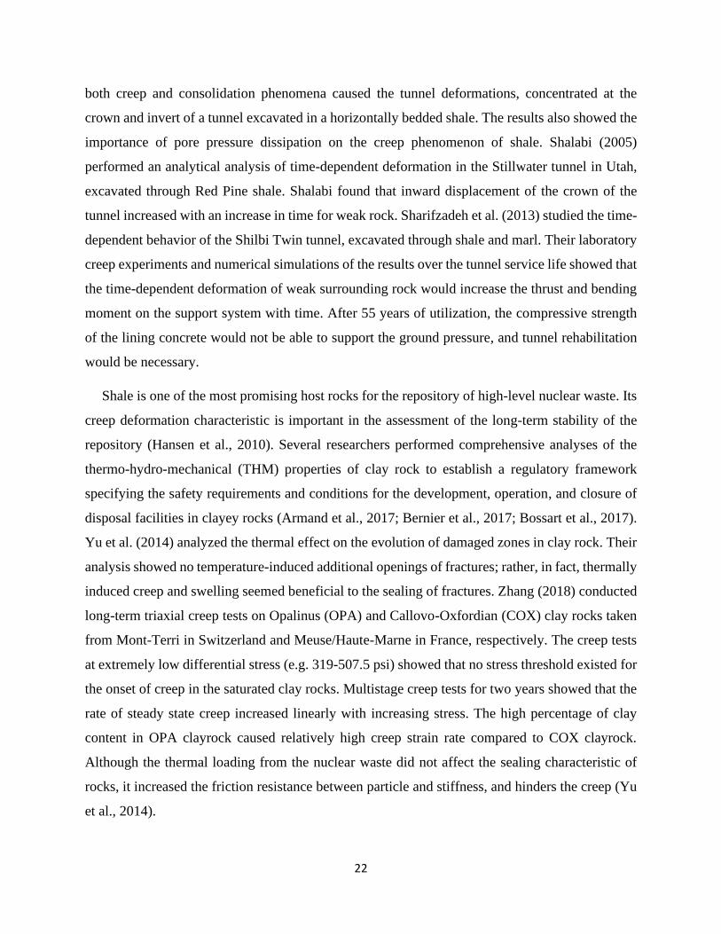
unloading of the axial stress. Price explained that, during the creep test, the inhomogeneous nature
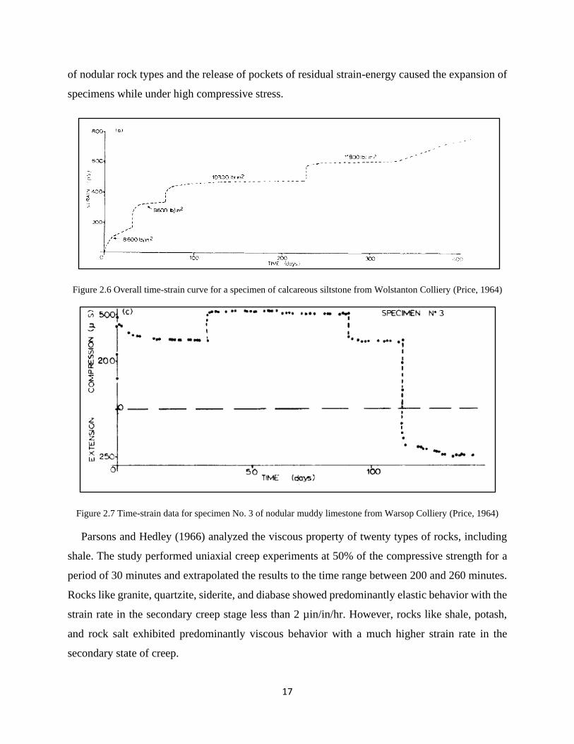
17
of nodular rock types and the release of pockets of residual strain-energy caused the expansion of
specimens while under high compressive stress.
Figure 2.6 Overall time-strain curve for a specimen of calcareous siltstone from Wolstanton Colliery (Price, 1964)
Figure 2.7 Time-strain data for specimen No. 3 of nodular muddy limestone from Warsop Colliery (Price, 1964)
Parsons and Hedley (1966) analyzed the viscous property of twenty types of rocks, including
shale. The study performed uniaxial creep experiments at 50% of the compressive strength for a
period of 30 minutes and extrapolated the results to the time range between 200 and 260 minutes.
Rocks like granite, quartzite, siderite, and diabase showed predominantly elastic behavior with the
strain rate in the secondary creep stage less than 2 µin/in/hr. However, rocks like shale, potash,
and rock salt exhibited predominantly viscous behavior with a much higher strain rate in the
secondary state of creep.

18
Hobbs (1970) conducted incremental uniaxial creep experiments on Hucknall shale, such that
uniaxial stress varied between 45% and 70% of the failure strength. Hobbs observed that the
magnitude of creep strain in Hucknall shale was equivalent to the instantaneous strain during
quasi-static loading. The empirical relationship between longitudinal strain and time is mentioned
in Equation 2.5. Here, l was longitudinal strain, t was time, and a, b, and c were empirical constants.
The creep recovery for the off-loaded specimen was appreciably less than the creep strain under
load, and the final permanent strain was about 35% of the maximum longitudinal strain under load.
Hobbs inferred that the recorded irrecoverable strain was relative to the applied stress, and neither
the instantaneous nor the primary strain under load were completely recoverable.
𝑙 = 𝑎 + 𝑏𝑡 + 𝑐2 ∗ 𝑙𝑜𝑔(𝑡 + 1) (2.5)
Singh (1975) conducted compressive-creep tests on Appin Colliery shale by an incremental
stress method, maintaining a particular stress on specimens for 2-3 hours (shown in Figure 2.8).
Unlike Price (1964), Singh observed an increase in the strain rate during the steady-stage of creep
with subsequent increments in applied stress. Singh also found that shale specimens failed along
their plane of weakness and concluded that these specimens experienced creep deformation along
the pre-existing plane of weakness, rather than the rock material itself. In addition, Singh
formulated the power creep law (Equation 2.6). Here, ε was strain, t was time, and a and b were
empirical constants.
𝜀 = 𝑎 ∗ 𝑡𝑏 (2.6)

19
Figure 2.8 Axial strain-time curve for Appin Colliery shale (Singh, 1975)
Cogan (1976) conducted laboratory creep tests on Ophir shale taken from the Burgin Mine of
the Tintic Division in Eureka, Utah. The creep failure of hard shale specimens was brittle and
varied from the development of a single crack at 50 psi confining stress to a distributed system of
hairline vertical cracks at 500 psi. The brittle behavior of rock means the continuous decrease in
the load supported by the rock as the strain increases (Jaeger, Cook, & Zimmerman, 1976).
Cogan’s tests showed a relationship between the primary and secondary stages of creep and the
volumetric change in the water saturated specimen. In the primary creep stage, a saturated
specimen consolidates, however, in the secondary stage, the volume of the specimen expands.
Cogan also found that the pre-consolidation of the saturated specimens reduced the sensitivity of
the creep strain rate to change in differential stress. Cogan’s research also showed that the level of
axial stress affected the consolidation stage of the specimen. For example, low axial stress caused
the consolidation to continue into the secondary stage of creep, while high axial stress immediately
terminated the consolidation state. Therefore, Cogan concluded that complex creep models were
essential in predicting the creep properties of shale around proposed underground openings.
Mishra and Verma (2015) performed laboratory creep tests on coal-measure shale taken from
the underground coal mines in West Virginia. Their experiments showed that laminated shale
specimen exhibits time-dependent deformation in both unconfined and confined stress conditions.

20
They concluded that the level of differential stress influences the level of creep strain and rate of
creep strain. Their experimental creep results also showed good fit to Norton’s creep law, shown
in Equation 2.7. Here, ε° is strain rate, σ is differential stress, p is an empirical exponent, and k is
an empirical constant.
𝜀° = 𝑘 ∗ 𝜎𝑝 (2.7)
These past works are examples of laboratory creep studies on coal measure shale. They detail
the influence of different levels of axial stress on the rate of creep strain, however, they did not
investigate the influence of other parameters, such as bedding planes, mineralogy, temperature,
water content.
2.2 Creep study in shale from oil wells, tunnels, and nuclear waste repository
Researchers in the oil and gas industry have extensively studied creep deformation in shale to
investigate the closure rate of hydraulic fractures. The research showed the influence of parameters
such as temperature, pore pressure, mineralogy, organic content, anisotropy, and stiffness on the
creep characteristics of shale. Chong et al. (1978) conducted uniaxial creep tests on oil shale
specimens, and their experimental results showed that the different stress levels and volumetric
organic content influenced the creep behavior of shale. Chu and Chang (1980) investigated the
influence of temperature on the creep behavior of oil shale, finding that temperature affected the
overall strength and Young’s modulus of oil shale. They noted that high temperatures increased
the rate of secondary creep strain. Rongzun et al. (1987) studied the influence of waterflooding on
the time-dependent strength of oil well casing in shale. The results of this study’s two non-linear
rheological models showed that higher water content in shale caused a higher formation creep
loading and increased the chances for casing collapse. Savage and Braddock (1991) studied the
influence of pore pressure on the rigidity and permeability of Pierre shale. Their hydrostatic tests
showed the variation in pore pressure, volumetric strain, and strain parallel and perpendicular to
the bedding orientation with time. They concluded that with increasing confining pressure, the
coefficient of consolidation and permeability decreased, however, the bulk moduli of Pierre shale
increased, possibly due to the closure of voids. Liu and Zhou (2000) investigated the change in
creep behavior of shale with water content and confining stress. The modes of failure changed
from shear flow to fracture network-shear failure to fracture network-plastic flow as the confining

21
pressure and water content increased, as shown in Figure 2.9. Sone (2012) investigated the
influence of carbonate and clay content on the creep characteristics of shale. Sone’s extensive
laboratory experiments on four different types of oil shale showed an inverse relationship between
strength and clay content. Sone and Zoback (2014) also concluded that creep deformation is an
inherent property of the dry rock, as it occurs in the absence of pore fluid. Khosravi (2017) showed
that creep behavior of shale depends on mineralogy, stress history, bedding plane orientation, and
temperature. Khosravi also found that the stiffness of the rock affects the creep deformation, as
shale rock with high instantaneous deformation also experienced high creep deformation.
Figure 2.9 Experimental observation on the relation between confining stress and failure modes for soft rock under
creep deformation (Liu and Zhou, 2000)
In tunneling, a rockmass that contains a considerable amount of clay, like shale, often shows a
time-dependent increase in the radial displacement of the tunnel walls (Barla et al., 2010). In the
situation of time-delayed deformation, the immediate installation of permanent lining restrains the
radial displacement and increases the support pressure acting on the lining. Lo et al. (1978)
analyzed the time-dependent behavior of shale rock taken from seven formations in southern
Ontario. They observed differences in the swelling characteristics of shale from the same
formations, influenced by the composition and clay fabric of the rock. Lo and Lee (1990) examined
the time-dependent deformational behavior of Queenston and southern Ontario Shale. Their
extensive tests at in-situ stress state showed that the swelling behavior of shale was orthotropic in
nature, which meant that the application of stress in one principal direction suppressed the swelling
phenomenon in all three orthogonal directions. Aristorenas (1992) studied the evolution of
deformation in tunnels excavated in two types of shales. The experimental findings concluded that
22
both creep and consolidation phenomena caused the tunnel deformations, concentrated at the
crown and invert of a tunnel excavated in a horizontally bedded shale. The results also showed the
importance of pore pressure dissipation on the creep phenomenon of shale. Shalabi (2005)
performed an analytical analysis of time-dependent deformation in the Stillwater tunnel in Utah,
excavated through Red Pine shale. Shalabi found that inward displacement of the crown of the
tunnel increased with an increase in time for weak rock. Sharifzadeh et al. (2013) studied the time-
dependent behavior of the Shilbi Twin tunnel, excavated through shale and marl. Their laboratory
creep experiments and numerical simulations of the results over the tunnel service life showed that
the time-dependent deformation of weak surrounding rock would increase the thrust and bending
moment on the support system with time. After 55 years of utilization, the compressive strength
of the lining concrete would not be able to support the ground pressure, and tunnel rehabilitation
would be necessary.
Shale is one of the most promising host rocks for the repository of high-level nuclear waste. Its
creep deformation characteristic is important in the assessment of the long-term stability of the
repository (Hansen et al., 2010). Several researchers performed comprehensive analyses of the
thermo-hydro-mechanical (THM) properties of clay rock to establish a regulatory framework
specifying the safety requirements and conditions for the development, operation, and closure of
disposal facilities in clayey rocks (Armand et al., 2017; Bernier et al., 2017; Bossart et al., 2017).
Yu et al. (2014) analyzed the thermal effect on the evolution of damaged zones in clay rock. Their
analysis showed no temperature-induced additional openings of fractures; rather, in fact, thermally
induced creep and swelling seemed beneficial to the sealing of fractures. Zhang (2018) conducted
long-term triaxial creep tests on Opalinus (OPA) and Callovo-Oxfordian (COX) clay rocks taken
from Mont-Terri in Switzerland and Meuse/Haute-Marne in France, respectively. The creep tests
at extremely low differential stress (e.g. 319-507.5 psi) showed that no stress threshold existed for
the onset of creep in the saturated clay rocks. Multistage creep tests for two years showed that the
rate of steady state creep increased linearly with increasing stress. The high percentage of clay
content in OPA clayrock caused relatively high creep strain rate compared to COX clayrock.
Although the thermal loading from the nuclear waste did not affect the sealing characteristic of
rocks, it increased the friction resistance between particle and stiffness, and hinders the creep (Yu
et al., 2014).

23
2.3 Application of rheological models to simulate creep deformation
Researchers have tried to predict the time-dependent behavior of shale through rheological
models. The rheological models assume that the time-dependent deformation is attributed to the
viscous nature of the material and each material deforms according to its intrinsic viscosity
(Aristorenas, 1992). The different types of rheological creep models are based on the appropriate
combination of three basic rheological elements: Hookean (spring), Newtonian (viscous dashpot),
and St. Venant element. To understand the complex rheological models, which simulate the
instantaneous and time-dependent deformation of shale, it is necessary to explain the meaning or
behavior of the basic rheological elements and models.
The Hookean element (shown in Figure 2.10 (a)) is a spring, which follows Hooke’s law (refer
to Equation 2.8). In rheological models, the modulus of stiffness (E) characterizes the Hookean
element. Physically, it represents the immediate strain (ε) in the material corresponding to applied
stress (σ). The Newtonian element (shown in Figure 2.10 (b)) is a viscous dashpot. The strain
induced in the Newtonian element is time-dependent; physically, it explains the creep phenomena
(refer to Equation 2.9). The coefficient of viscosity (η) characterizes the Newtonian element. The
St. Venant element is a combination of two plates with finite frictional resistance (σp) against each
other, as shown in Figure 2.10 (c). Equation 2.10 explains the stress-strain relationship of the St.
Venant element. It shows that if the applied stress (σ) is less than the frictional strength (σp) of the
St. Venant element, the induced strain (ε) is zero. However, if the applied stress is greater than or
equal to the frictional strength, the St. Venant element provides no resistance and the continuous
plastic flow occurs.
𝜎 = 𝐸 ∗ 𝜀 (2.8)
𝜎 = 𝜂 ∗ (𝑑𝜀
𝑑𝑡) (2.9)
𝜎 = 𝜎, 𝜀 = 0 𝑓𝑜𝑟 𝜎 < 𝜎𝑝
𝜎 = 𝜎𝑝, 𝜀 = 𝜀(𝜎) 𝑓𝑜𝑟 𝜎 ≥ 𝜎𝑝 (2.10)

24
Figure 2.10 Basic Rheological elements: (a) Hookean element; (b) Newtonian element; (c) St. Venant element
Based on the nature of strain developed in the rock, Aristorenas (1992) classified rheological
models into two categories: viscoelastic and viscoplastic models. In viscoelastic models, the
different combination of the Hookean and Newtonian elements provided four basic models:
Maxwell, Kelvin-Voigt, Poynting-Thomsen, and Burger. In the Maxwell model, the Hookean and
Newtonian elements are in series combination, as shown in Figure 2.11 (a). In this arrangement,
applied stress will immediately produce strain through the Hookean element that continuously
increases with time through the Newtonian element, as shown in Figure 2.11 (b). In the Kelvin-
Voigt model, the Hookean and Newtonian elements are in parallel combination, as shown in Figure
2.12 (a); therefore, this model does not show any instantaneous strain in response to the applied
stress. In fact, the viscous Newtonian element determines the rate of strain of the model, as shown
in Figure 2.12 (b), but the Hookean element determines the limit of the strain. In the Poynting-
Thomsen model, the Hookean element is in series to the Kelvin-Voigt model, as shown in Figure
2.13 (a). The strain response of this model is very similar to the Kelvin-Voigt model, except it also
shows the instantaneous strain in response to the applied stress through an independent Hookean
element in series, as shown in Figure 2.13 (b). In the Burger model, the Maxwell and Kelvin-Voigt
models are in series combination, as shown in Figure 2.14 (a). This combination represents three
types of strains: an immediate strain, a linear variation in strain, and exponential variation in strain
with time, as shown in Figure 2.14 (b). In terms of creep phenomena, the Poynting-Thomsen model
explains the instantaneous and transient creep stage, while the Burger model explains the
instantaneous, transient, and steady-state of creep. In fact, researchers widely use the Burger model
to explain the creep behavior of rocks (Price, 1964; Fakhimi and Fairhurst, 1994).
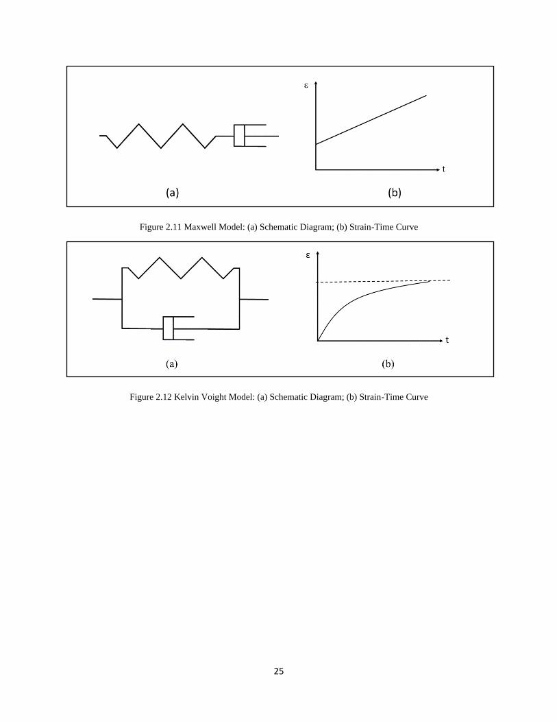
25
Figure 2.11 Maxwell Model: (a) Schematic Diagram; (b) Strain-Time Curve
Figure 2.12 Kelvin Voight Model: (a) Schematic Diagram; (b) Strain-Time Curve

26
Figure 2.13 Poynting Thomsen Model: (a) Schematic Diagram; (b) Strain-Time Curve
Figure 2.14 Burger Model: (a) Schematic Diagram; (b) Strain-Time Curve

27
In viscoplastic models, the St. Venant element represents the plastic strain in the model. Here,
the different combination of the basic rheological units provides the Bingham model. In the
Bingham model, the St. Venant element connects in parallel to the Newtonian element, as shown
in Figure 2.15 (a). This model shows no strain until the applied stress exceeds the resistance offered
through the St. Venant element and further accumulated strain releases as function of time through
the Newtonian element, as shown in Figure 2.15 (b). In addition, another combination of all three
rheological elements yields a series combination of the Burger and Bingham models, as shown in
Figure 2.16 (a). Here, the Burger model defines the primary and secondary creep stages and the
Bingham model defines the tertiary creep stage, as shown in Figure 2.16 (b).
Figure 2.15 Bingham Model: (a) Schematic Diagram; (b) Strain-Time Curve
Figure 2.16 Series Combination of Burger and Bingham Model: (a) Schematic Diagram; (b) Strain-Time Curve

28
The rheological constitutive models have also simulated the creep behavior of shale. For
example, viscoplastic and viscoelastoplastic constitutive models explained the triaxial creep
behavior of Tournemire shale, taken from the Tournemire formation in France (Rouabhi et al.,
2007; Li, Nguyen, Su, Labrie, & Barnichon, 2016). It also helped researchers to understand the
excavation distributed zone around the underground excavations of Tournemire shale. Pellet et al.
(2009) proposed a damageable viscoplastic constitutive law to understand the time-dependent
development of the excavation damage zone (EDZ) in argillaceous rock, such as shale. Both
viscoelastic and viscoplastic models explained the closure rate of hydraulic fractures in shale
formations. For example, Sone and Zoback (2011) used a viscoplastic constitutive model to
understand the time-dependent deformation in organic rich shale that influences the hydraulic
fracturing operations in shale gas reservoirs, proppant embedment, and permeability of the rock.
Guo and Liu (2012) used the Maxwell model to understand the depth of proppant embedment in
shale gas production. Li and Ghassemi (2012) proposed a linear viscoelastic Burger model to
understand the creep and closure rate of hydraulic fractures in shale; they also found that the
mineralogy influenced the elastic stiffness of the shale specimens. Almasoodi et al. (2014) studied
the unexpected early decline in the shale gas production through a viscoelastic constitutive model,
series combination of the Poynting-Thomsen and Kelvin Voigt. This model simulated the creep
behavior of the Eagle Ford shale and tested the interaction between the shale and different types
of fracturing fluids, such as water and decane.
Similarly, in tunnel excavations, rheological models predicted the deformation of tunnel walls
excavated in shale rock. For example, Aristorenas (1992) suggested an elastic-plastic creep
constitutive model, based on the drained and undrained creep experiments on Opalinus shale.
Bonini et al. (2009) presented a case study of a large size tunnel excavated through Apennines clay
shale, modeling its creep behavior using the visco-elastic plastic model and the elastic visco-plastic
Lemaitre’s model. Chen (2009) developed a visco-elastic creep model to investigate the long-term
behavior of tunnels excavated in weak rock, such as shale. Chen concluded that the creep
properties of the material should be considered in designing the tunnel support. Ghosh Roy and
Rao (2015) reviewed the validity of several constitutive models to simulate the creep behavior of
shale to understand the deformation of deep tunnels in Himalaya. Their experimental results
provided a threshold value of the creep stress; however, no single rheological model explained the
long-term behavior of the rock under various stresses and temperatures.

29
2.4 Creep in Ductile Rock Salt
The study of the time-dependent deformation in rock salt began in the early nineteenth century
to understand the formation of diapiric salt structures, or salt domes, in a sedimentary basin.
Previous theories suggested that the salt domes formed through 1) the deposition of salt from sea
water by volcanic heat and the force of crystallization pushing it upwards, or 2) tectonic activity,
or 3) the upward movement of salt into weak spots by overburden stress (Ode, 1968). Since the
information on the formation of salt domes came from observations in salt mines and geologic
inferences, many disputed the fundamental reason for salt domes formation. However, these
observations proved that rock salt can deform plastically and that its behavior is not brittle (Ode,
1968). In 1934, Nettleton experimentally presented the Arrhenius concept of gravitational
instability. Nettleton illustrated that the salt domes formed because their density was lower than
the overlying strata. The fundamental explanation assumed that salt deforms slowly under
differential stress, which depends on two primary factors: the contrast between the density of the
salt and overburden, and the creep properties of the salt. The viscosity of rock salt depends on
temperature, confining pressure, differential stress, time, and impurities, such as gypsum and
amount of water. As the creep of solid materials like rock and salt is complex, geologists did not
accept the Arrhenius’ idea of gravitational instability and relative difference in viscosity for a long
time.
Another reason for time-dependent study in rock salt was for the design of nuclear waste
repositories. The property of rock salt to creep under sustained load and seal cracks makes it a
suitable host rock for the disposal of nuclear radioactive waste (BGR, 2009). According to a US
National Academy of Sciences report, the disposal of nuclear waste must occur hundreds of meters
underground in specially constructed and mined openings, comprised of both natural and
engineered barriers to provide high levels of protection from the toxic effects of waste (Hess et al.,
1957). The two working examples of nuclear waste repository in rock salt are the Waste Isolation
Pilot Plant (WIPP) in Carlsbad, New Mexico, USA and the Endlager fur Radioactive Abfalle
Morsleben (ERAM) site in Morsleben, Germany. As such, the formation of salt domes and
assessment of long-term stability of nuclear waste repository pushed the study of creep
phenomenon in rock salt.
30
The behavior of crystalline salt masses closely resembles that of metals, like similar lattice
structures between certain metal crystals and sodium chloride crystals, as well as the ductile nature
of rock salt (Rinne, 1926). Triaxial experiments on salt crystals showed that both ductility and
ultimate strength increased with an increase in confining pressure. Therefore, the initial study of
creep in rock salt started with the knowledge of creep phenomenon in metal. The early research of
the creep phenomenon in rock salt began with laboratory experiments on single crystals of salts.
Reusch first observed plastic deformation in the single crystal of halite (Ode, 1968); Mugge and
Heide further confirmed this, stating that the mechanism of plastic deformation of salt depends on
temperature and pressure (Buerger, 1930). Stocke and Borchert (1936) performed two-hour creep
tests on rock salt at room temperature and atmospheric pressure. Griggs (1939) tested single
crystals of halite at room temperature and atmospheric pressure for 42 days loaded to 61 bars.
Griggs measured the elastic and inelastic deformation in the specimen and observed the diagonal
lines through the crystal, possibly due to plastic deformation. Kendall (1958) performed uniaxial
and triaxial creep experiments on cylindrical specimens of a single crystal of halite and Solenhofen
limestone at room temperature, with differential stress from 34.5 bars to 276 bars. The creep
experiments showed three types of deformation: instantaneous elastic strain, elastic flow, and
pseudoviscous flow, similar to the experimental observations of Griggs (1939). Kendall’s research
also showed that transient creep became non-existent with increasing confining pressure, such that
halite crystals became very plastic at high confining stress. Parker et al. (1959) tested natural dome
salt and bedded salt under uniaxial creep condition to determine the effect of nuclear waste
radiation on the creep behavior of salt. They found that at constant temperature, high radiation
doses did not change the structural properties of rock salt. However, high temperature increased
the rate of creep for both irradiated and unirradiated specimens. Brown and Jessen (1959) studied
the rate of closure of cavities in salt. They discovered that unless proper surface pressure relief
facilities were provided, one should only partially fill rock salt with nuclear waste due to its
inevitable creep characteristic. Their simulated high overburden pressure experiments showed the
complete closure of salt cavities due to plastic flow in rock salt. Serata (1959) performed creep
experiments on synthetic single crystal and fine-grained natural polycrystalline rock salt and
analyzed the influence of temperature, pressure, and saturated sodium chloride (NaCl) solution on
the creep properties of rock salt. Senseny (1985) showed that the rate of creep strain in bedded
rock salt exponentially increased with differential stress; in fact, at low stress, rock salt exhibited
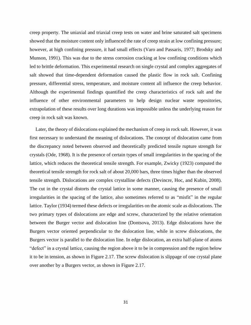
31
creep property. The uniaxial and triaxial creep tests on water and brine saturated salt specimens
showed that the moisture content only influenced the rate of creep strain at low confining pressure;
however, at high confining pressure, it had small effects (Varo and Passaris, 1977; Brodsky and
Munson, 1991). This was due to the stress corrosion cracking at low confining conditions which
led to brittle deformation. This experimental research on single crystal and complex aggregates of
salt showed that time-dependent deformation caused the plastic flow in rock salt. Confining
pressure, differential stress, temperature, and moisture content all influence the creep behavior.
Although the experimental findings quantified the creep characteristics of rock salt and the
influence of other environmental parameters to help design nuclear waste repositories,
extrapolation of these results over long durations was impossible unless the underlying reason for
creep in rock salt was known.
Later, the theory of dislocations explained the mechanism of creep in rock salt. However, it was
first necessary to understand the meaning of dislocations. The concept of dislocation came from
the discrepancy noted between observed and theoretically predicted tensile rupture strength for
crystals (Ode, 1968). It is the presence of certain types of small irregularities in the spacing of the
lattice, which reduces the theoretical tensile strength. For example, Zwicky (1923) computed the
theoretical tensile strength for rock salt of about 20,000 bars, three times higher than the observed
tensile strength. Dislocations are complex crystalline defects (Devincre, Hoc, and Kubin, 2008).
The cut in the crystal distorts the crystal lattice in some manner, causing the presence of small
irregularities in the spacing of the lattice, also sometimes referred to as “misfit” in the regular
lattice. Taylor (1934) termed these defects or irregularities on the atomic scale as dislocations. The
two primary types of dislocations are edge and screw, characterized by the relative orientation
between the Burger vector and dislocation line (Dontsova, 2013). Edge dislocations have the
Burgers vector oriented perpendicular to the dislocation line, while in screw dislocations, the
Burgers vector is parallel to the dislocation line. In edge dislocation, an extra half-plane of atoms
“defect” in a crystal lattice, causing the region above it to be in compression and the region below
it to be in tension, as shown in Figure 2.17. The screw dislocation is slippage of one crystal plane
over another by a Burgers vector, as shown in Figure 2.17.

32
Figure 2.17 Schematic representation of (a) edge and (b) screw dislocations in a cubic crystalline material, where
filled circles denote the lattice points of a crystal, b is a Burgers vector, hatched area and dashed line show the slip
plane and dislocation line, respectively (Dontsova, 2013)
Taylor (1934) showed that the plastic deformation of single crystals of metals and rock salt are
different; however, they possessed certain common characteristics. The single crystal in tension or
compression consists of shear strain and sheets of crystal parallel to a crystal plane slipping over
one another. Through a simple analytical atomic model, Taylor explained that there was a definite
temperature (TD) that was likely lower than the recrystallization temperature, allowing for the free
movement of unit dislocation along the crystal plane. At temperature above TD, any amount of
shear stress applied parallel to the slip plane would cause movement of dislocation in the direction
of applied stress. However, if the temperature was below TD, a finite value of shear stress was
necessary for the movement of dislocation. According to the theory of dislocations (Friedel, 1967;
Haasen, 1974; Anderson, Hirth and Lothe, 2017), irreversible or plastic deformation of crystals
results from the motion of dislocation on crystallographic plane. The application of finite shear
stress induces plastic flow in the crystal that multiplies the dislocations; in turn, their motion is
hindered due to mutual interactions. Therefore, an increase in shear stress is necessary to increase
the shear strain in the crystal.
Cristescu and Hunsche (1998) mentioned that, similar to the creep of metals (Haasen, 1974),
the creep of rock salt primarily occurred by transcrystalline dislocation movement, i.e., glide,
climb, and cross-slip, where at least five independent slip systems must be activated concurrently.
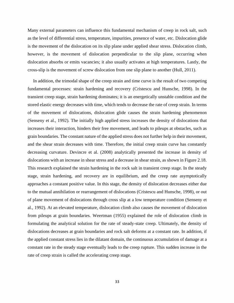
33
Many external parameters can influence this fundamental mechanism of creep in rock salt, such
as the level of differential stress, temperature, impurities, presence of water, etc. Dislocation glide
is the movement of the dislocation on its slip plane under applied shear stress. Dislocation climb,
however, is the movement of dislocation perpendicular to the slip plane, occurring when
dislocation absorbs or emits vacancies; it also usually activates at high temperatures. Lastly, the
cross-slip is the movement of screw dislocation from one slip plane to another (Hull, 2011).
In addition, the trimodal shape of the creep strain and time curve is the result of two competing
fundamental processes: strain hardening and recovery (Cristescu and Hunsche, 1998). In the
transient creep stage, strain hardening dominates; it is an energetically unstable condition and the
stored elastic energy decreases with time, which tends to decrease the rate of creep strain. In terms
of the movement of dislocations, dislocation glide causes the strain hardening phenomenon
(Senseny et al., 1992). The initially high applied stress increases the density of dislocations that
increases their interaction, hinders their free movement, and leads to pileups at obstacles, such as
grain boundaries. The constant nature of the applied stress does not further help in their movement,
and the shear strain decreases with time. Therefore, the initial creep strain curve has constantly
decreasing curvature. Devincre et al. (2008) analytically presented the increase in density of
dislocations with an increase in shear stress and a decrease in shear strain, as shown in Figure 2.18.
This research explained the strain hardening in the rock salt in transient creep stage. In the steady
stage, strain hardening, and recovery are in equilibrium, and the creep rate asymptotically
approaches a constant positive value. In this stage, the density of dislocation decreases either due
to the mutual annihilation or rearrangement of dislocations (Cristescu and Hunsche, 1998), or out
of plane movement of dislocations through cross slip at a low temperature condition (Senseny et
al., 1992). At an elevated temperature, dislocation climb also causes the movement of dislocation
from pileups at grain boundaries. Weertman (1955) explained the role of dislocation climb in
formulating the analytical solution for the rate of steady-state creep. Ultimately, the density of
dislocations decreases at grain boundaries and rock salt deforms at a constant rate. In addition, if
the applied constant stress lies in the dilatant domain, the continuous accumulation of damage at a
constant rate in the steady stage eventually leads to the creep rupture. This sudden increase in the
rate of creep strain is called the accelerating creep stage.

34
Figure 2.18 Evolution of shear stress (τ) and dislocation density (ρ) in slip system versus the total shear strain (γp) in
the Dislocation Dynamics Simulation of tensile deformation in copper crystals (Devincre et al., 2008)
Based upon the fundamental mechanism of creep in rock salt, researchers also proposed a
composite model to analyze the long-term safety of a permanent nuclear waste repository and to
predict the thermomechanical behavior of the surrounding host rock. The model treated the
material as a composite consisting of soft and hard regions, namely the subgrain interiors and the
subgrain boundaries, respectively. Researchers based this model on the physical processes
governing the deformation at the microscopic level. The research work of Weidinger et al. (1996;
1997) showed that this composite model allowed the reliable prediction of long-term behavior of
rock surrounding the permanent nuclear waste repository. As the composite model came from the
general physical principles of micromechanical deformation, the model was applicable for any
kind of crystalline material (Cristescu and Hunsche, 1998).
2.5 Creep in Brittle Quartz
In the upper Earth’s crust, most rocks accommodate deformation in a brittle manner (Brantut et
al., 2013). Once the rock reaches critical stress, brittle failure takes place either due to the
generation of a new fracture in intact rock or sliding along a pre-existing interface or shear fault
35
(Scholz, 2002; Patterson and Wong, 2005). Among the many factors affecting the brittle failure of
rocks, the least studied has been time. The time-dependent brittle deformation of rock, also referred
to as brittle creep, under constant stress holds importance in the study of the critically stressed, the
brittle Earth’s crust. It controls the precursory phase of several important geohazards (Main and
Meredith, 1991). Earthquake ruptures and volcanic eruptions are examples of the dynamic failure
of brittle Earth crust, taking place due to the relative slow deformation in a subcritically stressed
state (Heap, 2009). Creep deformation also holds importance in fault dynamics during earthquake
cycles. One such example is the change in static stress in a lobate pattern adjacent to faults
following an earthquake rupture (King et al., 1994). Although the stress change was very small,
only a few tenths of an MPa at a distance of a few kilometers, it had the potential of failure of any
fault strand within the stressed lobe (Brantut et al., 2013).
Brittle creep affects the overall strength of the Earth crust and causes rock deformation at lower
stresses. While it reduces the cohesion of intact rocks, it does not influence their internal friction
(Brantut, et al., 2013); this implies that friction controls the maximum long-term strength of the
crust. An appropriate laboratory experiment to study brittle creep would be to subject rock
specimens to a constant stress that is proportionally lower than their short-term strength and allow
them to deform naturally over time until, eventually, they fail (Brantut, et al., 2013). The constant
strain rate tests determine the short-term strength, typically at a strain rate of 10-5 s-1. Matsushima
(1960a) found that Shodoshima biotite granite experienced higher creep strain in the lateral
direction compared to the longitudinal direction. Roberston (1960) also found that, in creep
experiments, volumetric strain increased in the Solenhefen limestone specimens. Hobbs (1970)
performed uniaxial creep experiments on seven types of rocks, including Ormonde siltstone, Lea
Hall sandstone, and Portland limestone. Hobbs also recorded the increase in the volume of the
specimen during creep, and the volume prior to fracture was greater than the initial unloaded
volume. Therefore, the initial experimental creep studies on brittle igneous rocks suggested that
the volume of rock increases during creep.
Brittle rocks, such as quartz, granite, and marble, which are subjected to uniaxial or triaxial
stress state, can exhibit elastic behavior up to the stress level equivalent to 50% of the peak axial
strength. At the end of the elastic region, the volume of the specimen is minimum; at the point
when nonelastic behavior begins, the volume of the rock increases (Brace et al., 1966). As stress
36
increases and climbs to the fracture point, the rock expands more and more relative to the elastic
changes. Schock et al. (1973) defines the departure of the volumetric strain at a given mean stress
from that observed in hydrostatic loading as dilatancy. The stress level at the onset of dilatancy is
usually between one-third and two-thirds of the macroscopic fracture stress (Brace, 1978).
Ultrasonic wave measurements (Jones, 1952), special optical methods (Berg, 1950), strain gauges
(Blakey and Beresford, 1955), and direct observations of sectioned material (Hsu et al., 1963)
suggested that cracking precedes the fracture of concrete in uniaxial compression. Similarly, Brace
et al. (1966) analyzed the linear compressibility of Westerly granite in the axial and circumferential
direction and showed the formation of open axial cracks beyond the elastic range. The variation of
compressional wave velocity in the axial and radial directions also identified the formation of open
axial cracks (Tocher, 1957; Matsushima, 1960b; Scholz, 1968a). These experiments showed that,
after stress removal, the crack porosity was within the experimental error of the permanent increase
in the volume of the specimen. This finding proved that, in constant strain rate experiments, the
formation of open axial cracks caused the permanent volumetric deformation in the brittle rock,
which eventually led to failure.
Gold (1960) analyzed the creep behavior of ice under constant compressive load and detected
the cracking activity with piezoelectric crystals. Gold observed that the rate of crack formation
was proportional to the creep strain; specifically, it decreased as the creep rate approached a
constant. Above a certain stress, cracking continuously increased with the creep rate. Watanabe
(1963) studied the creep behavior of granite under compression and found that the creep strain was
directly proportional to the microcracking activity in the specimens. Wu and Thomsen (1975)
distinguished the three stages of creep in microcracking radiation in Westerly granite. They
explained that the first stage of creep involved closure of the microcracks that are perpendicular
or diagonal to the stress axis and opening of cracks that are parallel to the stress axis. In the second
stage of creep, stress-aided corrosion occurred, and cracks propagated. In the third stage of creep,
the coalescence of crack arrays occurred, and a weak zone or fault plane formed in the specimen.
This experimental research showed that the primary mechanism of creep in brittle rock is
microcracking.
The technique of microcrack observation developed with time. Adams and Williamson (1923)
first recognized the influence of void space or cavities on the physical properties of crystalline

37
brittle rocks, such as granite and diabase. They suggested that the tiny crackline voids in granite
increased its compressibility. Brace et al. (1972) used a simple physical model to study the
influence of microcavities in rock on elastic, thermal, electric, and other properties; this model
assumed the rock was a solid matrix with a dilute concentration of isolated cavities of circular or
elliptical cross section. However, the direct observation of cracks and pores was still unpopular,
partly because of their small size. Paulding (1965) observed transgranular cracks in undeformed
Westerly granite and crack growth in the direction parallel to the maximum compression using the
thin sections. Wawersik and Brace (1971) analyzed the polished sections of granite and diabase
deformed in the triaxial stress state; they observed that the distribution of microcracks depended
on the confining pressure. In the uniaxial or low confining state, local cracks were predominantly
parallel to the direction of maximum compression. However, at a confining pressure greater than
2,900 psi, local cracks predominantly inclined to the direction of maximum compression and of
macroscopic shear fracture. Additionally, at a very high confining pressure, local cracks tended to
propagate in their initial plane. Peng and Johnson (1972) analyzed the fracture propagation in thin
sections of Chelmsford granite using an 8 x binocular microscope to determine the length,
distribution, and preferred orientation of microcracks. Although these early researchers directly
analyzed the microcracks at higher resolution, the inevitable surface damage during the preparation
of thin sections caused ambiguous results for crack shape, length, and density. Standard techniques
of grinding and polishing rocks produced brittle cracks, local melting, or plastic flow, and leave
residual in the form of debris. In addition, the cracks observed were limited in size to about the
order of tenths of millimeters and important details were missed.
Brace et al. (1972) developed a new method of preparing thin sections to observe microcracks
better under an optical microscope or with a scanning electron microscope (SEM). The thin
sections were prepared in two steps: first, preparation of a finely ground surface, and second,
removal of the residual debris by ion thinning. This method produced fewer of the negative effects
of mechanical polishing, which did not influence the microscopic visualization using SEM. Sprunt
and Brace (1974) used this method on different types of brittle rocks and analyzed the various
types of grains, grain boundaries, high and low aspect ratio microcavities, crack lengths, and crack
apertures. Tapponnier and Brace (1976) investigated the stress-induced microcracks in Westerly
granite. SEM analyzed the thin-polished sections of the specimens, unloaded at successive stress

38
levels. They then correlated the crack development in the rock specimens to the stress-strain curve
and found that the dilatancy of their rock roughly coincided with the appearance of new cracks.
In 1979, Kranz investigated the growth and interaction of microcracks in Barre granite under a
constant stress state and correlated the observations with the creep strain and time curve. The
experimental methodology involved visualization and quantification of the microcracks in granite
specimens using a SEM. Kranz analyzed five granite specimens unloaded at successive time
intervals of creep strain and time, considering that each specimen was homogenous. In Figure 2.19,
specimen 30 was unstressed, and its quantitative results of microcracks were used as the baseline
to compare with the other specimens. Specimen 25 represented the stage when axial stress became
constant and the primary creep stage began. Specimen 27 represented the end of the primary creep
stage and the beginning of the secondary creep stage. Specimen 32 represented the end of the
secondary creep stage and the onset of the tertiary creep stage. Specimen 29 represented the tertiary
creep stage that lead to the inevitable failure of granite specimen. Figure 2.20 shows an example
of SEM imaging of granite specimens showing microcracks along the grain boundary of a feldspar
grain. Kranz showed that both the average length and the total length of microcracks increased
with the duration of creep experiment; however, the average width of microcracks remained
relatively constant. The average and total length of microcracks was highest in specimen 29,
followed by specimens 32, 27, 25, and 30. Based on these experimental findings, Kranz concluded
that the growth and development of microcracks caused the creep in the brittle granite. Atkinson
(1984) called this phenomenon sub-critical crack growth, or stable cracking.

39
Figure 2.19 Schematic representation of the experimental methodology of creep experiments on granite (Kranz,
1979)
Figure 2.20 Separation of two-feldspar grain through boundary in the vertical direction because of loading (Kranz,
1979)

40
Kranz (1979) also discussed the mechanistic reason for sub-critical growth of microcracks in
brittle rocks. Once a microcrack forms, the local stress drops in the vicinity of the microcrack. The
microcracks can only propagate in one of two conditions: one, the stress at the tip of microcrack
increases; or two, the strength of the tip of microcrack decreases. In the constant strain rate
compressive tests, the continuously increasing far-field stresses increases the local stress at the tip
of the microcracks, and the stress-induced microcracks grow to longer lengths in the direction of
the maximum compressive stress. However, in the creep test, the far field compressive stresses
remain constant, and the stress-induced microcracks can only propagate due to the decrease in
strength at the tip of the microcracks. Factors such as the interaction between two cavities,
temperature, and moisture (also called corrosive agents) decreases the strength at the tip of the
microcrack (Martin, 1972). Therefore, Kranz concluded that, in a constant stress state, the rate of
propagation of microcracks depends upon the rate at which corrosive agents decrease the strength
of the tip of microcracks.
Wawersik and Brown (1973) also studied the influence of confining stress on the creep strain
rate of sandstone and granite. They observed that the increase in confining stress decreases the rate
of secondary creep strain. Kranz (1980) showed that high confining stress increased the time-to-
reach failure of crystalline rock. Kranz proposed that high confining stress decreased the rate of
migration of corrosive agents at crack tips and decreased the crack interaction prior to reaching the
tertiary creep stage. Kranz et al. (1982) studied the influence of temperature on the creep behavior
of brittle rocks. The creep experiments on Barre granite showed that the time to reach failure
decreased by two orders of magnitude from 24°C to 200°C. These experimental studies explained
the creep phenomena of brittle rocks and the influence of extrinsic environmental factors.
2.6 Summary of the literature review
The literature review presented that, in different fields of engineering, studies have only
examined the creep phenomenon in shale using experimental and rheological methods. The
laboratory creep experiments showed that shale is a viscous rock that deforms at a constant stress
state, and the creep deformation is elastoviscous in nature. There are many extrinsic and intrinsic
parameters that influence the creep deformation in shale, such as level of differential stress,
confining stress, temperature, mineralogy, pore pressure, moisture content, orientation of bedding
planes, and stress history. The experimental investigation yielded both empirical and rheological

41
models (Challamel et al., 2005; Cristescu, 2012) that considered the physical characteristics of
shale to predict the time-dependent behavior. Although the previous researchers made successful
attempts in simulating the long-term response of shale, the fundamental mechanistic reason for
creep deformation is still unknown.
This review also detailed the available literature on the fundamental reason observed for creep
phenomenon in rock salt and quartz. In rock salt, the constant stress produced creep deformation
due to the movement of dislocations in the crystal lattice. The rate of movement of the dislocations
controls the rate of creep strain and causes the creep deformation and failure. The parameters, such
as level of differential stress, confining pressure, moisture content, and temperature directly
influence the motion and density of the dislocation. However, sub-critical crack growth is the
primary mechanism of creep deformation in brittle rocks, such as quartz and granite. The similar
parameters also control the growth of sub-critical cracks and influence the rate of steady-state and
time to reach failure in brittle rocks.
As such, this chapter presented that the reason for the gap in the fundamental knowledge of
creep in shale was the limited interpretation of creep phenomenon from the macroscopic
deformation at laboratory and field scale. However, the study of creep phenomenon in rock salt
and quartz showed that the fundamental reason of macroscopic creep deformation could be best
understood from the microscopic study of the rock deformation. Therefore, in a similar manner,
this research proposed to extend the microscopic study of creep to shale types sedimentary rocks
in order to understand the fundamental mechanical reason for creep in shale.

42
Chapter 3 Characterization of Mineralogy and Compressive Strength of Shale
This experimental investigation of creep phenomenon used Marcellus shale as its specimens.
Marcellus shale is an organic rich formation, belonging to the middle Devonian age unit of the
ancient sedimentary system, called the Appalachian Basin (Popova, 2017). As shown in Figure
3.1, the formation extends in the subsurface from New York State in the north to northeastern
Kentucky and Tennessee in the south, eastern Ohio to extreme western Virginia (Roen, 1984).
Marcellus shale is primarily composed of carbonaceous silty black shale with scattered pyrite,
scarce fossils, and carbonate concretions. Based on the variation in sea level during deposition, the
formation contains shale with different colors and interbedded limestone. The shale’s color ranges
from medium light gray to black that relays information about its depositional environment; for
example, Marcellus shale deposited in an oxygen-deficient environment is black in color with
significant organic content. The top elevation of the Marcellus formation varies from 1000 to -
8000 feet subsea depth (Popova, 2017). This negative elevation means that the top of the Marcellus
shale formation lies below the sea level. The thickness of the Marcellus shale formation varies
between 0 to 950 feet (Popova, 2017).
Figure 3.1 Index map of stratigraphic cross-sections and the Devonian Outcrop belt in the Appalachian Basin (Roen,
1984)
The current study obtained the Marcellus shale specimens from a Devonian outcrop located in
western New York. The specimens were light gray in color with no visible laminations. As shale

43
is an anisotropic rock, the coring direction of the specimens was parallel (PL) and perpendicular
(PD) to the orientation of bedding plane. This chapter briefly introduces the laboratory equipment
and procedures to determine the uniaxial and triaxial compressive strength of the shale specimens.
It also elaborates on the experimental procedure of X-ray powdered diffraction (XRD), as well as
the results of the mineralogy analysis of the Marcellus shale.
3.1 Uniaxial and Triaxial Compressive Strength Tests
This study conducted the uniaxial compressive strength (UCS) testing using servo-controlled
MTS-810 testing equipment, shown in Figure 3.2. The bottom steel platen of the MTS-810 uses a
linear variable differential transformer (LVDT) to measure the longitudinal displacement of the
platen during UCS testing. This LVDT was used to determine the axial displacement of the
specimen. As shown in Figure 3.3, a radial chain extensometer was mounted onto the specimen to
measure the radial strain during the UCS test. Since the rate of loading influences the compressive
strength of rocks (Rinehart, 1965), the rate of load application was determined according to the
American Society for Testing and Materials (ASTM) Standard-D7012 for quasi-static loading. By
applying stress to the specimens at quasi-static loading condition, the axial load increased at the
constant rate of 314 pounds per second (100 psi per second for 2.113 inches diameter).
Figure 3.2 Servo-controlled MTS-810 testing equipment and its components: (1) Load frame; (2) Hydraulic
actuator; (3) Strain gauge control panel; (4) MTS data acquisition system; (5) Computer; (6) Upper steel platen; (7)
Lower steel platen (Das, 2018)
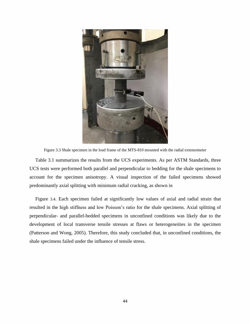
44
Figure 3.3 Shale specimen in the load frame of the MTS-810 mounted with the radial extensometer
Table 3.1 summarizes the results from the UCS experiments. As per ASTM Standards, three
UCS tests were performed both parallel and perpendicular to bedding for the shale specimens to
account for the specimen anisotropy. A visual inspection of the failed specimens showed
predominantly axial splitting with minimum radial cracking, as shown in
Figure 3.4. Each specimen failed at significantly low values of axial and radial strain that
resulted in the high stiffness and low Poisson’s ratio for the shale specimens. Axial splitting of
perpendicular- and parallel-bedded specimens in unconfined conditions was likely due to the
development of local transverse tensile stresses at flaws or heterogeneities in the specimen
(Patterson and Wong, 2005). Therefore, this study concluded that, in unconfined conditions, the
shale specimens failed under the influence of tensile stress.

45
Table 3.1 Results of unconfined compression strength test
Specimen
Type
Specimen
ID
L/D UCS
(Psi)
E
(KPsi)
Poisson’s
ratio
Strain at failure (%)
Axial Radial
Perpendicular
PD-1 1.99 16,289.3 2,589.7 0.09 0.0029 -0.0024
PD-2 1.98 8,414.35 3,778.7 0.14 0.0019 -0.0038
PD-3 1.99 10,867.75 2,173.55 0.29 0.0024 -0.0174
Parallel
PL-1 1.99 7,667.6 2,846.35 0.09 0.0015 -0.0012
PL-2 1.99 7,670.5 2,193.85 0.13 0.0021 -0.0026
PL-3 1.99 6,955.65 2,598.4 0.07 0.0021 -0.0027
Figure 3.4 Axial Splitting of Marcellus shale specimen under unconfined compressive stress (a) parallel-bedded, (b)
perpendicular-bedded

46
This study conducted triaxial compression strength experiments in the GCTS servo-controlled
RTX-1500 equipment, shown in Figure 3.5. By applying conventional triaxial stress, the major
principal stress (σ1) became greater than the minor principal stress (intermediate (σ2) = minor
principal stress (σ3)). The confining oil contained in the triaxial cell applied the circumferential
minor principal stress on the specimen. Sealing the specimen inside a polyolefin jacket helped to
prevent the contamination and absorption of confining oil in to the surface pores and cracks in the
specimen. Although the RTX-1500 has the frame LVDT to measure the longitudinal displacement,
direct mounting of both axial and lateral LVDTs onto the specimen enabled precisely determining
both the axial and lateral deformations. In the axial direction, there were two LVDTs mounted at
diametrically opposite sides, such that overall axial strain was the average value of the individual
axial LVDTs. The radial extensometer, mounted at the mid height of the specimen, measured the
radial strain. According to the ASTM standards, the loading was quasi-static in nature. Therefore,
the axial stress was increased at the constant axial strain rate of 10-5 per second. The procedure for
the triaxial strength test involved two stages. In the first stage, the specimen was consolidated by
increasing the axial and lateral stress hydrostatically up to the predetermined level of confining
stress. Once the triaxial cell attained the hydrostatic stress state, the confining stress remained
constant and the axial stress increased under a constant axial strain rate until the specimen failed.
In the triaxial strength experiments, four different confining pressures was selected to cover a
broad range of confinement in the rocks: 500 psi, 1,000 psi, 1,500 psi, and 2,000 psi. In addition
to failure strength, the elastic parameters as Poisson’s ratio (ν) and modulus of stiffness (E) were
also determined.
Figure 3.5 Laboratory setup of GCTS RTX-1500 (Mishra and Verma, 2015)

47
Table 3.2 summarizes the experimental results of the triaxial compressive strength tests. This
study considered the effect of specimen variation and heterogeneity on experimental results
through identical tests on two randomly selected shale specimens at each confining stress. The box
plot in Figure 3.6 shows that the confining pressure increased the average axial strength of both
types of shale specimens. Although the curve between average axial strength and confining
pressure was non-linear, the curve did not become concave towards the confining pressure axis;
this indicates that there was no transition from a brittle to a ductile failure mechanism (Patterson
and Wong, 2005). Figure 3.6 also shows that the mean axial strength of parallel and perpendicular
bedded specimens is comparable at different confining conditions. According to Hoek and Brown
(1980), the strength of a sedimentary rock depends on the angle between direction of major
principal stress and bedding plane (Figure 3.7), such that the strength is minimum at 30 degrees
and approximately similar at 0 and 90 degrees.
Table 3.2 Results of triaxial compressive strength tests
Specimen
Type
Specimen
ID
Axial
Strength
(Psi)
Confining
Stress
(Psi)
Modulus of
Stiffness (E)
(KPsi)
Failure
Angle
(degree)
Poisson’s
ratio
(ν)
Perpendicular
PD/5 14,232
500
4,460.2 15 0.11
PD/11 15,400 5,324.4 8 0.07
PD/4 18,683
1,000
5,325.8 15 0.09
PD/6 17,642 5,746.3 18 0.07
PD/7 21,485
1,500
6,213.2 18 0.02
PD/8 22,514 5,534.6 28 0.14
PD/9 25,226
2,000
5,782.6 30 0.02
PD/10 23,822 5,540.4 22 0.26
Parallel
PL/4 14,818
500
5,291 15 0.01
PL/5 14,197 5,724.6 10 0.27
PL/6 19,816
1,000
7,234 18 0.02
PL/7 19,566 6,404.6 20 0.28

48
PL/8 20,921
1,500
6,368.4 22 0.01
PL/9 20,055 6,407.5 30 0.33
PL/10 26,116
2,000
7,070.2 25 0.04
PL/11 23,970 6,890.4 28 0.31
Figure 3.6 Comparison of average axial strength at four different confining conditions in parallel- and
perpendicular- bedded shale specimens
Figure 3.7 Variation of axial strength with the orientation of discontinuity (Hoek & Bown, 1980)

49
In Figure 3.8, the axial stress-strain curve in the triaxial experiments shows that both types of
specimens experienced a sudden drop in strength beyond failure. The maximum axial strain at
failures was less than 0.5% for both types of specimen. In the post-failure state, the confining stress
stabilized the failure and each specimen reached a residual strength. Figure 3.8 also shows that an
increase in confining pressure increased the failure strength, residual strength, and axial strain at
failure; however, specimen failure remained brittle in nature.
(a)
(b)
Figure 3.8 Axial stress-strain curve in Triaxial Strength Test: (a) Parallel Specimen; (b) Perpendicular Specimen

50
In addition to the data analysis from the triaxial compressive strength tests, both types of
specimens were visually examined in the post-failure state. As shown in Figure 3.9, both parallel-
and perpendicular- bedded specimens failed due to the formation of shear failure planes. The
average angle of shear failure plane with respect to the direction of major principal stress (failure
angle) increased with the confining stress. According to Horii and Nemat-Naseer (1985), the
confining pressure inhibits the unstable growth of a single microcrack parallel to the direction of
axial stress, rather it allows the out-of-plane growth of a small microcrack to a finite length. The
constantly increasing axial stress led to the coalescence of small microcracks, and the specimen
fails along a macroscopic shear plane.
Figure 3.9 Failure of (a) Parallel-bedded, (b) Perpendicular-bedded shale specimen along shear plane under triaxial
compressive stress
3.2 Mineralogy of Marcellus shale through X-ray powdered diffraction
X-ray powder diffraction (XRD) analysis is a non-destructive technique that can accurately
determine the mineralogy of a rock sample (Ottner et al., 2000). The XRD equipment generates
X-rays in a sealed tube under vacuum. In the tube, current heats the filament that produces
electrons. The high voltage applied within the tube accelerates the electrons that hit the target made

51
of copper and generates X-rays. The X-ray beam interacts with the crystal lattice of the sample,
diffracting part of the beam. The detector senses the diffracted X-ray signal, processed either by a
microprocessor or electronically, and converts it into a count rate. The difference in the typical
diffraction pattern for each mineral allows identifying different minerals in the rock sample (Flohr,
1997).
XRD analysis was performed using the PANalytical XRD instrument, shown in Figure 3.10,
located in the shared research facility of West Virginia University. The XRD machine contains a
45-position specimen holder and a theta-theta goniometer. With the theta-theta goniometer, the
specimen surface is always horizontal and the X-ray source and the detector each moves in theta-
theta rotation about the specimen (Scintag, 1999). The equipment operated at a voltage of 45
kilovolts and 20 milli-ampere current. The specimen was mounted onto the spinning sample stage.
Figure 3.10 PANalytical X'Pert Pro X-ray Diffractometer (Das, 2018)
According to Pecharsky and Zavalij (2009), only the specimen containing an infinite number
of individual particles can provide a true powdered diffraction pattern. The reason for this is that
an infinite number of particles provide a completely random distributions of crystallographic

52
orientations of grains with respect to one another. Pecharsky and Zavalij suggested that, as the
ideal situation is not possible, the specimen should have a form of fine powder with the average
particle size between 10 and 50 microns. Therefore, the XRD analysis was conducted on powdered
shale specimens.
This study used five shale specimens that had failed under unconfined axial stress for the
powdered XRD analysis, reducing the solid pieces of shale specimens to the required small size
through the chronological steps of crushing, grinding, and sieving, separately. A jaw crusher,
shown in Figure 3.11(a), performed the primary crushing of the solid specimens. While keeping
the opening between the lower ends of the jaws to a minimum, the process of crushing produced
specimens with diameters sized between 5 and 20 mm. In the next step of specimen grinding, a
laboratory ball mill, shown in Figure 3.11(b), pulverized small pieces of rock into powder using
mechanical forces of impaction, compression, shearing, and attrition. The Ball mill consisted of a
steel grinding vessel of 11 inches in diameter that rolled on the drive. The rotating speed of the
drive was 132 rpm; as such, the grinding vessel was rotating at the speed of 60 rpm. The grinding
vessel contained rock pieces and solid steel balls that were 5 inches in diameter in the ratio of 4:1
for efficient mill grinding. The ground product was screened from the Ball mill through a No. 325
sieve (45 microns) using a RO-TAP sieve shaker, shown in Figure 3.11(c). After this process, five
powdered shale specimens sized less than 45 microns, shown in Figure 3.11(d), were collected.

53
Figure 3.11 Step-wise reduction of solid rock specimen into the powder sized less than 45 microns; (a) Jaw crusher;
(b) Ball mill; (c) RO-TAP sieve shaker; (d) Powder form of shale specimen
Following the standard operating procedure for the PANalytical X’Pert Pro XRD (2014), the
powdered shale specimen was filled into the specimen holder. Figure 3.12(a) shows the specimen
preparation kit for powdered specimens. The empty specimen holder ring clamped onto the
specimen preparation table. After filling the powdered specimen into the empty holder ring, the
powder press block pressed the specimen. The excess powder from the specimen, which flowed
out of the ring was cleaned up using the Stanley knife blade and dusting brush. Furthermore, the
bottom plate of the holder ring was clamped, and the complete specimen holder was removed by
turning the specimen preparation table upside down and pressing the spring-loaded knob. Figure
3.12(b) shows the specimen holder filled with powdered specimen. This method of specimen

54
preparation for XRD experiment is called the “backloading’ technique. The backloading technique
is the most accurate method for specimen preparation for XRD experiments because it minimizes
the preferential orientation of grains in the specimen and does not harm the specimen
characterization (Silva et al., 2011).
Figure 3.12 (a) Different parts of the specimen preparation kit; (b) specimen holder filled with powdered specimen
The X-ray detector captured the diffracted beam from the powdered specimen and processed
the detected signal by converting the intensity of diffracted X-ray into a count rate per second. In
the output, the detector produced an X-ray diffractogram, the curve between peak position and the
angle between incident and diffracted X-ray (Degree 2-theta), as shown in Figure 3.13. The X’Pert
High Score Plus software matched the recorded peaks in the X-ray diffractogram with the known
minerals through the American Mineralogist Crystal Structure Database or the Powder Diffraction
File (PDF) from International Centre for Diffraction Data. Table 3.3 summarizes the results of the
XRD experiments on the five powdered shale specimens. The average mineralogy showed that the
Marcellus shale had calcite as the primary constituent, 75.14% by weight. The shale also had minor

55
amounts of quartz, pyrite, and illite. These XRD results exhibited good consistency with the
published data of XRD analysis on the similar outcrop Marcellus shale specimens by Lora (2015).
Figure 3.13 X-ray Diffractogram of Marcellus shale specimen
Table 3.3 Mineralogy of Marcellus shale
Specimen ID
Carbonate Tectosilicates Clay
Calcite (%) Quartz (%) Pyrite (%) Illite (%)
PD-1
85 7 2 6
PD-2
74.3 11.8 2 11.9
PL-1
64.4 6.9 6.9 21.8
PL-2
84 5 2 9
PL-3 68 13 3 16
Average
Composition 75.14 8.74 3.18 12.94
56
3.3 Summary
The uniaxial and triaxial compressive strength tests showed that each specimen experienced a
sudden decrease in strength beyond failure. In triaxial compressive tests, the increase in confining
pressure increased the axial strength and axial strain at failure. As the axial strain at failure was
significantly small, the brittle-ductile transition (Heard, 1960) was not witnessed for the confining
pressure ranged from 500 to 2,000 psi. Therefore, the compressive strength tests showed that
Marcellus shale is a hard rock with axial strain less than 2% at failure under uniaxial compression
(ASTM, 2016), and failure remained brittle at high confining stress of 2,000 psi. In addition, the
mineralogy assessment through powdered XRD experiments showed that Marcellus shale is a
carbonate rock from composition. It contained significantly high percentage of calcite, and minor
amount of illite, quartz and pyrite. According to Ding et al. (2011), the brittle nature of Marcellus
shale was attributed to the high percentage of calcite that increased the stiffness and decreased the
Poisson’s ratio of the specimens. Therefore, in current chapter, the laboratory experiments
characterized the deformational nature of shale specimens.

57
Chapter 4 Triaxial Creep Test on Bedded Marcellus Shale
The permanently supported roofs of underground coal mines experience continued
deformation, or creep, under the influence of vertical and horizontal stresses. In addition to the
real-time monitoring of creep deformation of roof through instrument roof bolts (Benmokrane, et
al., 1995), laboratory testing is also an important method to analyze the creep properties of rock
(Zhang, et al., 2015). According to ASTM (2016), a triaxial creep test on intact rock core
specimens in the laboratory provides the quantitative parameters and, if utilized with proper
judgement, can determine the long-term stability of permanent underground structures. Therefore,
this study conducted laboratory creep experiments in the triaxial stress state to understand the creep
behavior of Marcellus shale and to better understand creep in coal mine roofs.
4.1 Experimental procedure of triaxial creep experiments
Triaxial creep experiments were conducted in the servo-controlled, GCTS triaxial test system
(RTX-1500). The procedure for the triaxial creep experiments included two stages in addition to
the initial hydrostatic consolidation of the specimen at the desired confining pressure. In stage 1,
the confining pressure remained constant and the axial stress increased at a constant rate of 70
psi/second until it reached the predetermined value of axial stress, which was smaller than the
failure strength. In stage 2, the axial stress remained constant until the specimen entered the tertiary
creep stage.
In the current research, triaxial creep experiments was conducted at two successive levels of
differential stress: 75% and 85% of the expected (differential) failure strength at each of four
confining pressures, e.g. 500, 1,000, 1,500, and 2,000 psi. Differential stress levels were selected
such that the creep experiments complete within a reasonable experimental duration (Kranz and
Scholz, 1977). According to Heap (2009), in triaxial creep experiments, the level of differential
stress should lie between the yield and dilation stress. As shown in Figure 4.1, points C’ and D’
on the differential stress and volumetric strain curve represented the level of yield stress and
dilation stress, respectively. Similarly, in this study, the yield and dilation stress levels were
determined at each of the four confining pressures from the previous triaxial compression strength
tests.

58
Figure 4.1 Stress-strain curve for Darley Dale sandstone (Heap, 2009)
As studies have associated microcracking with the deformation of brittle rock under
compression (Scholz, 1968a), Kranz and Scholz (1977) suggested a hypothesis of critical crack
density to characterize the onset of the tertiary creep stage in brittle rock. According to their
hypothesis, brittle rock enters the tertiary creep stage when it has acheived a critical value of
inelastic volumetric strain. Griggs (1940) first proposed the idea of a critical value of strain during
creep tests on water-saturated alabaster specimens. Later, Cruden (1974) showed that, if failure
was due to the coalescence of cracks, the critical strain could imply the critical crack density in
brittle rocks. Kranz and Scholz (1977) suggested that, in uniaxial stress condition, the inelastic
volumetric strain at any particular instant of time was the difference between the total and the
elastic volumetric strain, as mentioned in Equation 4.1. Equations 4.2 and 4.3 determined the total
and elastic volumetric strains, respectively. The symbols ΔV/V, εz, εr, and Δ represented volumetric
strain, axial strain, radial strain, and inelastic volumetric strain at time instant t, respectively; and
E, ν, and σ represented modulus of elasticity, Poisson’s ratio, and uniaxial stress, respectively.
∆(𝑡) = (∆𝑉(𝑡)
𝑉) − [
1−2∗ 𝜈
𝐸] ∗ 𝜎 (4.1)
(∆𝑉(𝑡)
𝑉) = 𝜖𝑧(𝑡) + 2 ∗ 𝜖𝑟(𝑡) (4.2)
𝜖𝑧 =𝜎
𝐸= −
𝜖𝑟
𝜈 (4.3)

59
As the current creep experiments were triaxial in nature (σ1 >> σ2 = σ3), the inelastic volumetric
strain was determined at the onset of tertiary creep stage using Equation 4.4, where σ1 and σ3
represented axial and confining stress, respectively.
∆(𝑡) = (∆𝑉(𝑡)
𝑉) −
[(𝜎1+2∗𝜎3)∗(1−2∗𝜈)]
𝐸 (4.4)
4.2 Results of triaxial creep experiments
Triaxial creep experiments were conducted on twenty-eight bedded shale specimens at eight
different triaxial stress states. Table 4.1 summarizes the value of the applied triaxial stresses, the
time to reach the tertiary creep stage (Tf), and remarks on the experiments. Eight specimens from
both variations of bedding orientation failed before reaching the predetermined level of differential
stress. In addition, three specimens, PL-20, PL-21, and PL-34, stressed for 463.42, 953.06, and
721.15 hours, respectively, did not enter the tertiary creep stage. In addition, the specimens under
similar levels of triaxial stress required different amounts of time to reach the onset of tertiary
creep. For example, in parallel-bedded specimens PL-15 and PL-25, it took 144.15 and 305.06
hours, respectively, to reach the tertiary creep stage at the same differential stress equivalent to
85% of failure strength. Similarly, among the perpendicular-bedded specimens, PD-15 and PD-32
took 159.49 and 1.48 hours to reach the onset of tertiary creep stage, respectively, at the same
differential stress equivalent to 85% of failure strength.
Table 4.1 Details of triaxial creep experiments on bedded Marcellus shale
Specimen
ID
Differential
Strength
(psi)
Confining
Stress
Percentage of
Differential
Stress (%)
Time to reach
tertiary creep
stage (Tf) (hours)
Remarks
PL-18 14,007 500 86.23 58.46 Entered tertiary creep stage
PL-19 500 76.21 64.86
PL-20 1,000 76.29 463.42 Did not enter tertiary creep stage
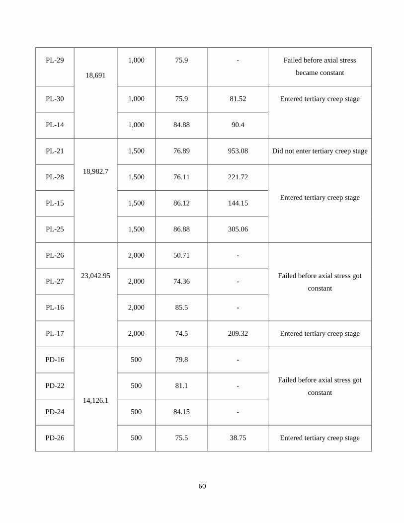
60
PL-29
18,691
1,000 75.9 - Failed before axial stress
became constant
PL-30 1,000 75.9 81.52 Entered tertiary creep stage
PL-14 1,000 84.88 90.4
PL-21
18,982.7
1,500 76.89 953.08 Did not enter tertiary creep stage
PL-28 1,500 76.11 221.72
Entered tertiary creep stage PL-15 1,500 86.12 144.15
PL-25 1,500 86.88 305.06
PL-26
23,042.95
2,000 50.71 -
Failed before axial stress got
constant PL-27 2,000 74.36 -
PL-16 2,000 85.5 -
PL-17 2,000 74.5 209.32 Entered tertiary creep stage
PD-16
14,126.1
500 79.8 -
Failed before axial stress got
constant PD-22 500 81.1 -
PD-24 500 84.15 -
PD-26 500 75.5 38.75 Entered tertiary creep stage

61
PD-21 500 84.5 11.71
PD-27
17,162.8
1,000 75.09 250.76 Entered tertiary creep stage
PD-33 1,000 75.42 0.63
PD-34 1,000 75.45 721.15 Did not enter tertiary creep stage
PD-15 1,000 86.7 159.49 Entered tertiary creep stage
PD-32 1,000 86.9 1.48
PD-28 20,499.4 1,500 75.02 3.49 Entered tertiary creep stage
PD-18 1,500 86.9 66.24
PD-23
22,518.05
2,000 73.5 20.53 Entered tertiary creep stage
PD-20 2,000 85.5 - Failed before axial stress got
constant
The time to reach the onset of tertiary creep was compared with the level of differential stress
at different confining conditions. Figures 4.2 and 4.3 show graphical comparisons for parallel- and
perpendicular-bedded shale specimens, respectively. The similar comparison for creep tests on
Barre granite is presented in Figure 4.4 (Kranz, 1980). It shows that the coefficient of
determination (R2) is significantly high for Barre granite specimens at four different confining
conditions. However, for Marcellus shale, the value of R2 is very small, varied between 0.0429 and
0.2481. It indicates that the level of differential stress did not influence the time to reach failure
for both parallel and perpendicular bedded shale specimens. In Figures 4.2 and 4.3, the value of
R2 is 1 only for two data points at specific confining pressure.

62
Figure 4.2 The comparison between the time to reach the onset of tertiary creep stage and level of differential stress
in parallel-bedded specimens
Figure 4.3 The comparison between the time to reach the onset of tertiary creep stage and level of differential stress
in perpendicular-bedded specimens

63
Figure 4.4 Logarithm of the failure time in seconds versus stress difference in kilobars at confining pressure of 1 bar,
530 bars, 1000 bars, and 1980 bars(Kranz, 1980). Best fit, least squares regression lines and R2 are shown
In Equation 4.3, Kranz and Scholz (1977) determined the modulus of elasticity (E) and
Poisson’s ratio (ν) from separate constant strain rate tests on brittle rocks. As the behavior of the
shale specimens in this testing was very heterogeneous, this study determined the E and ν
separately for each creep test to calculate the inelastic volumetric strain. The secant modulus of
elasticity and Poisson’s ratio was calculated between zero and the axial stress equivalent to 40%
of the failure strength (ASTM, 2014). Since the current creep experiments were triaxial, Equation
4.4 was used to determine the inelastic volumetric strain at the onset of tertiary creep stage. Table
4.2 summarizes the results of E, ν, rate of secondary creep strain, and inelastic volumetric strain at
the onset of tertiary creep stage.
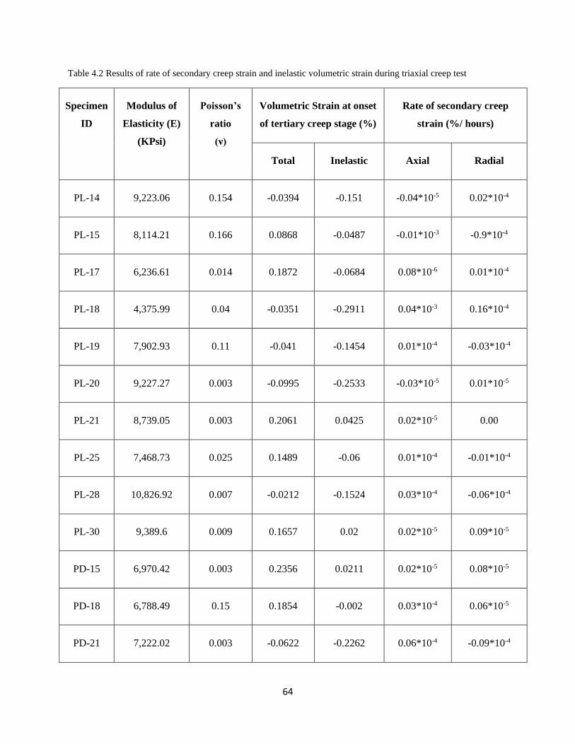
64
Table 4.2 Results of rate of secondary creep strain and inelastic volumetric strain during triaxial creep test
Specimen
ID
Modulus of
Elasticity (E)
(KPsi)
Poisson’s
ratio
(ν)
Volumetric Strain at onset
of tertiary creep stage (%)
Rate of secondary creep
strain (%/ hours)
Total Inelastic Axial Radial
PL-14 9,223.06 0.154 -0.0394 -0.151 -0.04*10-5 0.02*10-4
PL-15 8,114.21 0.166 0.0868 -0.0487 -0.01*10-3 -0.9*10-4
PL-17 6,236.61 0.014 0.1872 -0.0684 0.08*10-6 0.01*10-4
PL-18 4,375.99 0.04 -0.0351 -0.2911 0.04*10-3 0.16*10-4
PL-19 7,902.93 0.11 -0.041 -0.1454 0.01*10-4 -0.03*10-4
PL-20 9,227.27 0.003 -0.0995 -0.2533 -0.03*10-5 0.01*10-5
PL-21 8,739.05 0.003 0.2061 0.0425 0.02*10-5 0.00
PL-25 7,468.73 0.025 0.1489 -0.06 0.01*10-4 -0.01*10-4
PL-28 10,826.92 0.007 -0.0212 -0.1524 0.03*10-4 -0.06*10-4
PL-30 9,389.6 0.009 0.1657 0.02 0.02*10-5 0.09*10-5
PD-15 6,970.42 0.003 0.2356 0.0211 0.02*10-5 0.08*10-5
PD-18 6,788.49 0.15 0.1854 -0.002 0.03*10-4 0.06*10-5
PD-21 7,222.02 0.003 -0.0622 -0.2262 0.06*10-4 -0.09*10-4

65
PD-23 8,104.17 0.009 0.2093 0.0165 -0.05*10-4 0.03*10-4
PD-26 7,248.55 0.001 -0.1365 -0.2826 -0.05*10-4 -0.05*10-4
PD-27 6,374.88 0.003 0.2385 0.043 0.01*10-4 -0.01*10-5
PD-28 10,573.46 0.02 0.1691 0.0339 2.6*10-4 -0.5*10-4
PD-32 13,033.28 0.008 -0.0854 -0.1991 -0.55*10-4 -2.55*10-4
PD-33 7,027.52 0.014 -0.1928 -0.367 -1.02*10-4 5.02*10-4
PD-34 5,927.12 0.004 0.2197 0.0091 -0.09*10-6 -0.01*10-5
The creep strain versus time curve in Figure 4.5 shows that brittle shale did not experience the
significant primary stage of creep deformation. In either directions, the creep strain remained in
steady stage and increased at a very slow rate until the onset of tertiary creep stage. Figure 4.5 also
shows that, except for specimens PL-14, PL-19, and PD-23, the onset of tertiary creep stage either
first appeared on the radial creep strain curve, or sometimes simultaneously on both the axial and
radial strain curves.

66

67

68
Figure 4.5 Creep strain versus time curve for bedded shale specimens
This study analyzed the relationship between secondary creep strain rate and applied differential
stress in the axial and radial direction. The available dataset was fitted to Norton’s creep law,
mentioned in Equation 4.5. The logarithm of Equation 4.5 transformed the power law into a linear
equation, mentioned in Equation 4.6. Figures 4.6 and 4.7 show the relationship between the
logarithm of axial and radial creep rate with the logarithm of differential stress, respectively.
𝑑𝜖
𝑑𝑡= 𝜖𝑠𝑠
° = 𝐴 ∗ 𝜎𝑛 (4.5)
log 𝜖𝑠𝑠° = log 𝐴 + 𝑛 ∗ log 𝜎 (4.6)
Where: 𝑑𝜖
𝑑𝑡 = 𝜖𝑠𝑠
° = rate of secondary creep strain in either direction
A, n = material constants
𝜎 = applied differential stress

69
Figure 4.6 Fitting of linear trend between log (axial creep rate) and log (differential stress) for bedded shale
specimens
Figure 4.7 Fitting of linear trend between log (radial creep rate) and log (differential stress) for bedded shale
specimens

70
The linear equations in Figure 4.6 and Figure 4.7 show that the degree of determination (R2)
was very low between the logarithm of secondary creep rate and the logarithm of differential stress.
In addition, in Figure 4.6, the slope of the best-fit linear equation was negative (-10.812) for
perpendicular-bedded specimens, implying that the rfate of axial creep rate decreased with the
increase in the differential stress. The poor value of R2 for all four equations suggested that the
secondary creep strain rate did not follow Norton’s creep law. We believe that the inherent
heterogenoity of intact core specimens is a primary reason of this discrepancy.
This study also analyzed the relationship between the inelastic volumetric strain at the onset of
tertiary creep stage with the level of confining stress. Figure 4.8 shows the results compared to the
similar analysis on Barre granite. In Barre granite, the inelastic volumetric strain increased towards
dilation with an increase in confining pressure for both the constant-rate fracture (strength) and the
creep tests. However, this phenomenon was not the same for our shale specimens. As shown in
Figure 4.9(a), in the parallel-bedded specimens, the inelastic volumetric strain increased towards
dilation in the strength tests, and toward compression in creep tests. However, in the perpendicular-
bedded specimens (Figure 4.9(b)), the inelastic volumetric strain increased towards compression
in both the constant strain rate and the creep tests. This result implies that, unlike Barre granite,
the axial compression dominated over the radial dilation and signficantly contributed towards the
onset of the tertiary creep stage in bedded shale specimens.
Figure 4.8 Dilatant volumetric strain at the onset of the tertiary creep stage as a function of confining pressure. Open
symbols represent constant-rate fracture tests; closed symbols represent creep tests. Error bars are standard deviation
and compression is negative (Kranz, 1980)

71
(a)
(b)
Figure 4.9 The relationship between inelastic volumetric strain and confining pressure in constant strain rate and
creep tests for: (a) parallel-bedded specimens; (b) perpendicular-bedded specimens

72
4.3 Summary
The triaxial creep experiments showed that the shale specimens experienced time-dependent
deformation under a constant stress state and, without prior warning, instantaneously entered the
tertiary creep stage of failure. However, the level of differential stress did not seem to influence
the time to reach failure. A few specimens did not enter the tertiary creep stage of deformation.
The steady state of creep deformation did not follow Norton’s creep law; the rate of secondary
creep strain in the axial and radial directions did not show a correlation with the differential stress.
Unlike the creep behavior of quartz and granite, the inelastic volumetric strain increased towards
compression with the increase in confining stress for the Marcellus shale specimens. Therefore,
the current experiments proved that brittle shale exhibited time-dependent deformation; however,
the nature of the creep deformation was erratic and did not necessarily obey previous empirical
creep law.

73
Chapter 5 Procedure of X-ray Computed Tomography (CT) Scanning and
Image Processing to Analyze Geometry of Microcracks
The X-ray computed tomography (CT) technique is a useful method for the non-destructive,
three-dimensional imaging and characterization of rock properties, such as fracture geometry, pore
network, inclusions of heterogeneous minerals, etc. (Deng et al., 2016). The application of the X-
ray CT technique has extensively solved the engineering problem of characterizing rock properties
and fluid flow in a porous medium (He, 1998). This application has also been beneficial with
valuable unique specimens, such as meteorites (Gnos et al., 2010) and fossils (Rowe et al., 2001).
Sellars et al. (2003) used the X-ray CT technique during triaxial stress application to cubic quartzite
specimens and studied the fracture development. Lenoir et al. (2007) used the X-ray CT technique
to visualize the shear deformation of argillaceous rocks under triaxial compression. Jia et al. (2014)
used the X-ray CT technique for three-dimensional (3D) imaging of fractures in carbonate rocks.
Yang et al. (2016) investigated a coalfield fire by analyzing the fractures due to high temperature
in anthracite and mudstone using the X-ray CT technique.
This chapter first introduces the operating procedures for X-ray CT equipment used in current
research. Furthermore, this chapter discusses the limitations of conventional image processing
techniques to analyze the X-ray CT images. It also elaborates on the workflow of a new image
processing technique using the built-in plugins in the open-source image analysis software, FIJI
(Schindelin, et al., 2012). In addition, this chapter explains the process of data extraction of the
geometry of microcracks using FIJI. The FIJI results for microcrack geometry are also compared
with another commercial image analysis software, Bruker Computed Tomography Analyser
(CTAn), in terms of accuracy and time for computational analysis.
5.1 Introduction of X-ray CT Equipment
An X-ray CT scan is a non-destructive, direct imaging technique, which visualizes cracks at the
micrometer level of magnification. The Industrial X-ray CT scanner has an X-ray source located
opposite to an X-ray detector with the specimen located in between, such that either the specimen
rotates 360 degrees, or both the source and detector rotate 360 degrees around the specimen
(Rodriguez et al., 2014). The X-ray CT produces images based on the transmittance of the X-ray
through a specimen. The density, thickness, and composition of the specimen determine the
intensity of the transmitted X-ray that passes through to the detector. Equation 5.1 details the

74
relationship between the intensity of the incident and the transmitted X-rays, also called the Beer-
Lambert Law, where the linear attenuation coefficient (µ) depends on the material density and
mass absorption coefficient (Karacan, 2003). In the X-ray CT image, minerals with high density,
thickness, and a high atomic number block a larger portion of X-ray energy than minerals with
lower density, thinness, and a low atomic number (Xradia, 2010). Therefore, the low-density areas
(e.g. cracks) appeared dark, while high-density areas (e.g. intact rock) appeared bright in color, as
shown in Figure 5.1.
𝐼
𝐼𝑜= exp (−𝜇ℎ) (5.1)
Figure 5.1 X-ray CT image with crack and intact rock
In this study, a NorthStar Imaging (NSI) M-5000 Industrial CT scanner imaged the cylindrical-
shaped shale specimens. X-ray CT scanner used in this research is located at the National Energy
Technology Laboratory (NETL) facility in Morgantown, West Virginia. As shown in Figure 5.2,
the core specimen was placed on a rotating platform between the X-ray source and detector, such
that the X-ray source and detector remained stationary and the specimen rotated 360 degrees. The
resolution of the scanner depends on the size of the specimen, ranging between 5–40 microns in
each of three mutually perpendicular directions.

75
Figure 5.2 NorthStar Imaging M-5000 Industrial CT scanner: (a) X-ray detector with vertical sandstone core, (b) X-
ray source with vertical sandstone core (Rodriguez et al., 2014)
Specimen thickness or density influences the penetration values of X-rays (i.e. the percentage
of detector counts around and through the specimen). Typically, a penetration value between 10%
and 90% results in good scan quality (Plessis et al., 2017). As the thickness of shale specimen was
2.113 inches, the operating condition of 185 kilovolts voltage and 400 microamperes current was
appropriate to enter the specimen and maintained the best balance of resolution and energy. The
X-ray CT scanner captured 1,440 radiographs during one complete rotational scan, such that it
captured each radiograph at 0.25-degree rotations of the specimen. In this analysis, the X-ray CT
equipment scanned the entire length of the specimen in two separate scans, with the results being
stitched together at a later stage (Crandall et al., 2018). NSI’s Efx-dr software reconstructed the
radiographs of each scan and produced two-dimensional (2-D) grayscale images, as shown in
Figure 5.3(a). The sequential stacking of the 2-D circular X-ray CT images reconstructed the 3-D
image of the specimen, as shown in Figure 5.3(b). The pixel resolution of the 2-D X-ray CT image
and the spacing between two consecutive planar grayscale images was 29.9 microns (µm).

76
Figure 5.3 (a) Two-dimensional grayscale image from X-ray CT scan of shale specimen; (b) Three-dimensional
image reconstructed from the stack of two-dimensional images
5.2 X-ray computed tomography (CT) image processing
An image is a definite array of pixels containing digital information of the scanned object. The
process of converting an image into a digital form to extract useful information is known as image
processing (Bernasconi, 2005). In this study, the X-ray CT scanner produced 2-D grayscale images
of the shale specimen, termed the Original Image, as shown in Figure 5.3(a). The original X-ray
CT image contained information on microcracks, such as aperture, length, area, etc., collectively
called the “geometry” of the microcracks. The main purpose of image processing in this analysis
was the conversion of the original grayscale image into a binary image that only contained
microcracks in the foreground (black color) and intact rock in the background (white color). First,
conventional image processing techniques were used, such as global thresholding and adaptive
thresholding, to generate the binary images of microcracks and analyze their efficiency and
limitations. Next, a new workflow for image processing was proposed and its operating procedure
is briefly detailed. This study used the FIJI software for image processing for both conventional
and the newly proposed methods.

77
5.2.1 Image processing using Global Thresholding technique
In global thresholding, one can extract a desired feature from an image background by
comparing the intensity of a pixel with only one threshold value selected for the entire image
(Sonka et al., 1999). The technique of global thresholding assumes that the grayscale image has a
uniform distribution of intensity. In FIJI, the plugin subroutines, Auto Threshold, performed the
global thresholding of the 8- or 16-bit grayscale image. Unlike the thresholder applet accessed
through FIJI > Adjust > Threshold where thresholding algorithms are selected manually, the
plugin automatically determined the threshold value for each available algorithm. The plugin
generated a montage of binary images of four rows × four columns that was the result of global
thresholding through sixteen available algorithms, such as Default, Huang, Otsu, Shanbag, etc.
Figure 5.4(a) shows the original X-ray CT image of the shale specimen, while Figure 5.4(b) shows
the result of Auto Threshold on this image for the 16 algorithms. The results showed that only four
algorithms, namely Li, Mean, Otsu, and Percentile, could show a few microcracks in the binary
image. However, the results of binary image suffered from the “beam-hardening” artifact that
caused the non-segmentation of microcracks in the middle region of the image.
Figure 5.4 (a) Original grayscale X-ray CT image; (b) Results of Global Thresholding through different algorithms

78
In the X-ray CT image, an incident X-ray beam attenuates while passing through the material.
At a suitable range of energy, the rate of attenuation depends on the composition and density of
the material. In the laboratory, the incident X-ray is a polychromatic beam (a range of the energy
spectrum) that does not attenuate uniformly while passing through an object. Therefore, even in a
homogenous object, the 2-D grayscale image contains brighter pixels at the edge and darker pixels
in the middle region of the image due to the range of frequencies in the X-ray beam. This artifact
is known as the “beam-hardening” artifact (Mohapatra, 2012). The artifact generates or implies
false information about the specimen composition and density. Although the X-ray CT image
reconstruction software pre-corrected the artifact, the residual beam-hardening artifact restricted
the segmentation of microcracks in the middle region of the image.
5.2.2 Image processing using Adaptive (Local) Thresholding technique
As the original X-ray CT image possessed the beam-hardening artifacts, the grayscale image
contained a non-uniform distribution of intensity. Therefore, the single threshold value in the
global thresholding technique did not provide good segmentation results for an entire image. In
the current method, an adaptive (local) thresholding technique was used to segment the
microcracks. Unlike global thresholding with one threshold value for an entire image, local
thresholding divided an image into subimages and calculated the threshold for each subimage
(Chow and Kaneko, 1972). In FIJI, the plugin Auto Local Threshold performed the adaptive
thresholding of the original grayscale image through nine different algorithms, such as Bernsen,
Contrast, Otsu, Sauvola, etc. The plugin computed the threshold for each pixel within the local
domain, specified by the radius of the window. Figure 5.5(a) shows the original X-CT image, while
Figure 5.5(b) shows the result of Auto Local Threshold on the original X-CT image. The results
showed that, except for algorithms Phansalkar and Sauvola, each of seven algorithms segmented
microcracks and generated a binary image. Although the texture and morphology of microcracks
were visible, the binary images contained a lot of noise. In addition, the result of the Contrast
algorithm suffered with the beam-hardening artifact and the microcracks in the middle region were
still indistinguishable. Therefore, the correction of the beam-hardening artifact and low-contrast
between object and background were essential pre-processing steps for the image segmentation
with these shale specimens.

79
Figure 5.5 (a) Original grayscale X-ray CT image; (b) Results of Adaptive Thresholding through different
algorithms
5.2.3 Image processing using Adaptive Thresholding technique on pre-processed X-ray CT
image
The pre-processing steps for the original X-ray CT image were the correction of the beam-
hardening artifact and an increase in contrast between microcracks and intact rock matrix. The
beam-hardening artifact caused brighter pixels at the edges and darker pixels in the middle region
of the image of a homogenous specimen. Romano et al. (2018) developed a plugin for the
automated beam-hardening correction in an X-ray CT image. The plugin runs on FIJI software on
both the individual and stack of X-ray CT images. To analyze the efficiency of this beam-
hardening correction, first the intensity of the beam-hardening artifact was determined in the
original grayscale image. The variation in the profile of gray-scale value (GSV) across the width
of the image is a suitable indicator of the beam-hardening artifact (Mohapatra, 2012). Figure 5.6
compares the GSV of the original and beam-hardening corrected (B-Hc) X-ray CT image across
the image width. The results showed that the profile of GSV for the original X-ray CT had a
cupping artifact, initially decreasing and then increasing with minimum GSV at the middle pixel
of the image (Mohapatra, 2012). Although the beam-hardening correction plugin reduced the mean
GSV of the original X-ray CT image, the profile of GSV for the B-Hc X-ray CT image was

80
approximately constant across the image width. This result shows that the beam-hardening
correction plugin effectively removed the beam-hardening artifact from the original X-ray CT
image. In the next step of pre-processing, the contrast between microcracks and the intact rock
matrix in the B-Hc X-ray CT image was improved through image smoothing. The filters, such as
mean or median smoothing sharpen the peaks of the unimodal histogram, make it more strongly
bimodal and allow better selection of a threshold for image segmentation (Lester et al., 1980;
Schmid, 1999). The mean filter is a sliding-window spatial filter that replaces the center value in
the window with the average of all pixel values in the window (Sakthivel & Prabhu, 2014).
However, in median filter, the value of center pixel is replaced by the median value of all pixel
values in the window. Here, the window is usually square of N by N size; N = 3, 5, 7 etc. In
particular, the median filter works well for the features like fractures in the image; unlike the mean
filter, it does not blur the edges of fracture. Therefore, in this study, the median filter improved the
contrast between features of B-Hc X-ray CT image.
Figure 5.6 Comparison of the GSV across the Image Width: (a) Original X-ray CT Image; (b) Beam-Hardening
corrected X-ray CT Image

81
In FIJI, the plugin Auto Local Threshold segmented the pre-processed B-Hc X-ray CT image.
Figure 5.7(b) shows the result of the image segmentation. The comparison of the results in Figure
5.5(b) and Figure 5.7(b) showed that pre-processing of the original X- ray CT image improved the
image segmentation; except for the Phansalkar and Sauvola algorithms, microcracks were more
visible using each of the seven other algorithms. For example, the results of algorithm Contrast on
the original X-ray CT image suffered from the beam-hardening effect; however, similar algorithms
showed all microcracks in the B-Hc X-ray CT image. Although the quality of image segmentation
improved through pre-processing, the output binary images from adaptive thresholding were not
directly useable for further analysis. The binary images required post-processing for background
noise removal. In addition, binary images from each of the seven algorithms contained noise in
form of rings that indicated the presence of ring artifacts (Boas & Fleischmann, 2012) in the B-Hc
X-ray CT images.
Figure 5.7 (a) B-Hc X-ray CT image; (b) Results of Adaptive Thresholding through different algorithms
5.2.4 Image processing using new proposed workflow in FIJI
Based upon the results of three different conventional techniques, it was concluded that the
original grayscale image had low contrast between microcracks and intact rock. The image also
suffered from the residual beam hardening and ring artifacts. Therefore, the first task was to

82
improve the contrast between microcracks and intact rock. In FIJI, the option called
“Brightness/Contrast” allows the manual adjustment of brightness and contrast in the original X-
ray CT image, as shown in Figure 5.8. Although the manual adjustment of brightness/contrast
showed the invisible microcracks in the image, the beam-hardening artifact caused the non-
uniform distribution of intensity. The region in the center appeared darker in color compared to
the edges of the image. Therefore, in this current analysis, the contrast of the original X-ray CT
image was adjusted using contrast limited adaptive histogram equalization (CLAHE).
Figure 5.8 Manual Adjustment of Brightness/Contrast of original X-ray CT Image
Unlike other contrast enhancement methods, such as linear unsharp masking or histogram
equalization, CLAHE did not increase noise in the original grayscale image and increased the
contrast (Nithya et al., 2014; Yadav et al., 2014). CLAHE is an improved version of the adaptive
histogram equalization (AHE) method that enhances contrast in local regions of the image
(Zuidervald, 1994). FIJI has this plugin pre-installed. CLAHE did not require the correction of
beam-hardening artifact in the original X- ray CT image while enhancing the local contrast. Figure
5.9 shows the comparison of the GSV across the image width at three different contrast levels.
Figure 5.9(a), 5.9(b), and 5.9(c) represented the distribution of GSV across the original X-ray CT
image, manually adjusted brightness/contrast in the original X-ray CT image, and the local contrast
enhanced X-ray CT image, respectively. Figure 5.9 shows that the original X-ray CT image had
beam-hardening or cupping artifact that increased upon the manual adjustment of
brightness/contrast. Although the local contrast enhancement increased the ring artifacts in the

83
image, it removed the cupping artifact. In addition, the microcracks were easily visible in the
contrast enhanced image compared to the original or manual brightness/contrast adjusted image.
The appropriate parameter values in the CLAHE plugin was determined through numerous
iterations that remained constant for the contrast enhancement of each image of different shale
specimens.
Figure 5.9 Comparison of GSV along the purple line among similar X-ray CT images at different contrast levels. (a)
Original X-ray CT image; (b) Manually Adjusted Brightness and Contrast in Original X-ray CT image; (c) Local
contrast enhancement in Original X-ray CT image
After pre-processing the original X-ray CT image in terms of contrast enhancement, the next
step of image processing was the segmentation of the microcrack. The plugin named trainable
weka segmentation (TWS) in FIJI segmented the contrast enhanced X-ray CT image into a binary
image with microcracks in the foreground. The plugin is a combination of a machine-learning
algorithm and a set of selected image features that produces pixel-based segmentation (Arganda-
Carreras, et al., 2017). By default, the plugin started with two classes to produce a binary image in
the output, such as microcracks and intact rock in Figure 5.10(a). The traces were added to both
classes using the tools for region of interest (ROI) available in FIJI. The traces possessed the
information of intensity of the pixels belonging to the class of microcrack and intact rock. For
example, as shown in Figure 5.10(a), the freehand selection tool (red color) traced the microcracks,
while the oval selection tool (green color) traced the intact rock in the contrast enhanced X-ray CT

84
image. After adding the traces to both classes, the plugin trained the input image through the option
Train Classifier and generated an image classifier. The image classifier stored the cluster of
intensity values of microcracks and intact rock and performed the unsupervised image
segmentation on other, untrained input images. For example, as shown in Figure 5.10(b), the
classifier generated an output image with red colored microcracks and green colored intact rock.
The next step was to convert the colored-output image into a binary image using the option Make
Binary, such that the microcracks were black colored features in the foreground and intact rock
was a white colored feature in the background, as shown in Figure 5.10(c). The biggest advantage
of TWS was that it allowed the user to finely discriminate different features into different classes
by tracing a reasonable number of ROIs (Arena, Piane, & Sarout, 2014), which also improved the
accuracy of image classifier. The results of binary images in Figure 5.4(b), Figure 5.5(b), Figure
5.7(b), and Figure 5.10(c) showed that the TWS efficiently segmented microcracks in the original
X-ray CT image. This current analysis, after several iterations, generated an appropriate image
classifier that remained constant for the image processing of all shale specimens. Therefore, the
two-step workflow of image processing, shown in Figure 5.11, proved efficient in the generation
of binary images of microcracks.
Although the plugin TWS produced directly useable binary images, sometimes binary images
possessed noise of sparsely occurring black pixels. This type of noise is also called salt-and-pepper
noise (Guo, Qu, Du, Wu, & Chen, 2014), where black and white pixels occur randomly in the
image. The function named Remove Outliers in FIJI eliminated the noise in the binary image
(Ferreira & Rasband, 2012). As the presence of noise is subjected to the nature of the contrast
enhanced X-ray CT image, the standard workflow of the new image processing technique did not
include this step.

85
Figure 5.10 Process of Trainable Weka Segmentation: (a) Tracing of Microcracks and Intact Rock in Contrast
Enhanced X-ray CT Image; (b) Colored Segmentation of X-ray CT Image; (c) Binary-Microcracks Segmented X-
ray CT Image

86
Figure 5.11 Workflow of new proposed image processing technique
5.2.5 Automation of image processing in FIJI
In this study, the average length and diameter of a cylindrical shale specimen was 4.2 inches
and 2.113 inches, respectively. The industrial X-ray CT equipment produced 2-D grayscale
images, such that the distance between two consecutive images was 29.9 microns. Therefore, based
on the length of the specimen and the separation between two consecutive images, the X-ray CT
scan produced approximately 3,500 images for each shale specimen.
The comparisons of binary microcracks images generated from conventional image processing
techniques and the new proposed method showed that the new proposed technique was efficient
and accurate in image processing. As the thickness of each specimen was constant, the distance of
each specimen from X-ray source and detector during scanning remained same. This method
produced a similar range of GSV for intact rock and microcracks in different shale specimens.
Therefore, the parameters of the new image processing workflow in plugin CLAHE and TWS
remained the same to generate the binary microcrack images for the different shale specimens.
Since the steps of image processing were constant for different specimens, a macro was written
in FIJI that expedited and automated the image processing. The macro mentioned in Appendix A
automatically opened the original 2-D X-ray CT images in FIJI, enhanced the contrast using
CLAHE, and saved the image in the output directory with a name similar to the original X-ray CT
image. This macro further generated the binary microcrack image using the TWS plugin through
the image classifier and saved the output image in another directory with a name similar to the
original X-ray CT image. Both contrast enhancement and image segmentation took 1.5 minutes
(approximately) for each image and took 87.5 hours for the complete specimen.

87
5.3 Geometry of microcracks from binary X-ray CT images
As mentioned above, X-ray CT equipment generated 3,500 grayscale images of the shale
specimen. The macro in Appendix A processed each image and generated 2-D binary images of
microcracks. Figure 5.12(a) shows the result of the automated image processing as a montage of
binary images spaced at 2.97 mm, representing the portion of the specimen. The 2-D binary images
from the top left to the bottom right show the variation in the geometry of microcracks along the
length of the specimen. Furthermore, the sequential stacking of 2-D binary images spaced at 29.7
microns reconstructed the 3-D microcracks, as shown in Figure 5.12(b). As the X-ray CT image
processing and reconstruction showed the distribution of microcracks in both 2-D and 3-D
coordinate systems, the geometry of microcracks was determined in both 2-D and 3-D, separately.
This analysis first determined the geometry of microcracks using FIJI and compared the results
with Bruker CTAn, in terms of accuracy and time efficiency.
Figure 5.12 (a) Montage of 2-D binary X-ray CT images spaced at 2.97 millimeters; (b) 3-D microcracks
reconstructed from 2-D binary images spaced at 29.7 microns
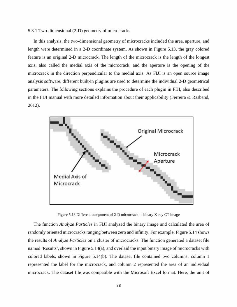
88
5.3.1 Two-dimensional (2-D) geometry of microcracks
In this analysis, the two-dimensional geometry of microcracks included the area, aperture, and
length were determined in a 2-D coordinate system. As shown in Figure 5.13, the gray colored
feature is an original 2-D microcrack. The length of the microcrack is the length of the longest
axis, also called the medial axis of the microcrack, and the aperture is the opening of the
microcrack in the direction perpendicular to the medial axis. As FIJI is an open source image
analysis software, different built-in plugins are used to determine the individual 2-D geometrical
parameters. The following sections explains the procedure of each plugin in FIJI, also described
in the FIJI manual with more detailed information about their applicability (Ferreira & Rasband,
2012).
Figure 5.13 Different component of 2-D microcrack in binary X-ray CT image
The function Analyze Particles in FIJI analyzed the binary image and calculated the area of
randomly oriented microcracks ranging between zero and infinity. For example, Figure 5.14 shows
the results of Analyze Particles on a cluster of microcracks. The function generated a dataset file
named ‘Results’, shown in Figure 5.14(a), and overlaid the input binary image of microcracks with
colored labels, shown in Figure 5.14(b). The dataset file contained two columns; column 1
represented the label for the microcrack, and column 2 represented the area of an individual
microcrack. The dataset file was compatible with the Microsoft Excel format. Here, the unit of
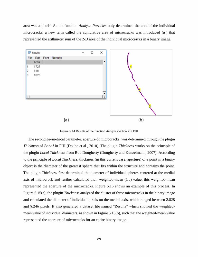
89
area was a pixel2. As the function Analyze Particles only determined the area of the individual
microcracks, a new term called the cumulative area of microcracks was introduced (ac) that
represented the arithmetic sum of the 2-D area of the individual microcracks in a binary image.
Figure 5.14 Results of the function Analyze Particles in FIJI
The second geometrical parameter, aperture of microcracks, was determined through the plugin
Thickness of BoneJ in FIJI (Doube et al., 2010). The plugin Thickness works on the principle of
the plugin Local Thickness from Bob Dougherty (Dougherty and Kunzelmann, 2007). According
to the principle of Local Thickness, thickness (in this current case, aperture) of a point in a binary
object is the diameter of the greatest sphere that fits within the structure and contains the point.
The plugin Thickness first determined the diameter of individual spheres centered at the medial
axis of microcrack and further calculated their weighted-mean (twm) value, this weighted-mean
represented the aperture of the microcracks. Figure 5.15 shows an example of this process. In
Figure 5.15(a), the plugin Thickness analyzed the cluster of three microcracks in the binary image
and calculated the diameter of individual pixels on the medial axis, which ranged between 2.828
and 8.246 pixels. It also generated a dataset file named “Results” which showed the weighted-
mean value of individual diameters, as shown in Figure 5.15(b), such that the weighted-mean value
represented the aperture of microcracks for an entire binary image.
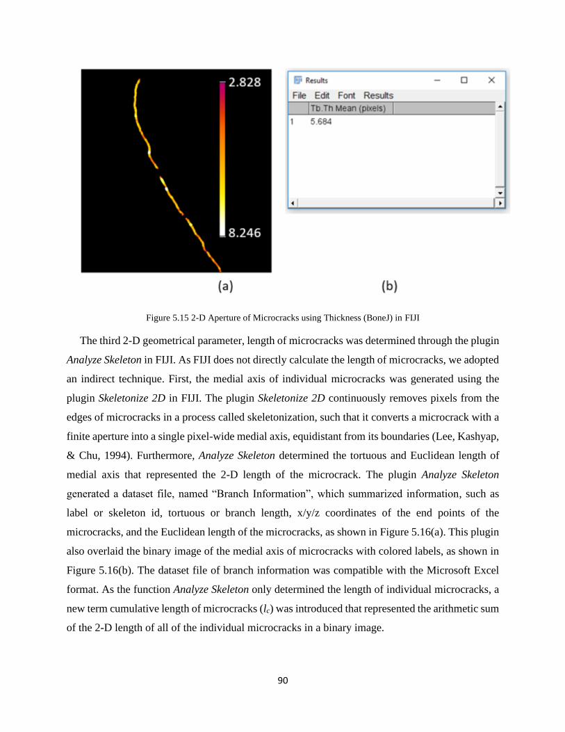
90
Figure 5.15 2-D Aperture of Microcracks using Thickness (BoneJ) in FIJI
The third 2-D geometrical parameter, length of microcracks was determined through the plugin
Analyze Skeleton in FIJI. As FIJI does not directly calculate the length of microcracks, we adopted
an indirect technique. First, the medial axis of individual microcracks was generated using the
plugin Skeletonize 2D in FIJI. The plugin Skeletonize 2D continuously removes pixels from the
edges of microcracks in a process called skeletonization, such that it converts a microcrack with a
finite aperture into a single pixel-wide medial axis, equidistant from its boundaries (Lee, Kashyap,
& Chu, 1994). Furthermore, Analyze Skeleton determined the tortuous and Euclidean length of
medial axis that represented the 2-D length of the microcrack. The plugin Analyze Skeleton
generated a dataset file, named “Branch Information”, which summarized information, such as
label or skeleton id, tortuous or branch length, x/y/z coordinates of the end points of the
microcracks, and the Euclidean length of the microcracks, as shown in Figure 5.16(a). This plugin
also overlaid the binary image of the medial axis of microcracks with colored labels, as shown in
Figure 5.16(b). The dataset file of branch information was compatible with the Microsoft Excel
format. As the function Analyze Skeleton only determined the length of individual microcracks, a
new term cumulative length of microcracks (lc) was introduced that represented the arithmetic sum
of the 2-D length of all of the individual microcracks in a binary image.

91
Figure 5.16 2-D Length of Microcracks using Analyze Skeleton in FIJI
The above paragraphs explained the application of different plugins in FIJI to calculate the 2-
D geometry of microcracks for one binary image. As there were approximately 3,500 binary
images of microcracks for one shale specimen, another macro in FIJI was used to expedite the
process of data extraction. The macro, mentioned in Appendix B, analyzed each binary image of
microcracks individually from an input directory, generated the dataset file of area, weighted-mean
aperture, and length of microcracks, and stored it in a .csv format in separate output directories.
The name of each type of dataset file was similar to the name of the input binary image. In the
output, the total number of dataset files was three times the number of the input binary images, i.e.
10,500 dataset files. MATLAB was used to condense the 10,500 dataset files into a single file that
contained information about the title of the input binary image, image ID, cumulative area,
weighted-mean aperture, and cumulative length of microcracks. The script in MATLAB
(mentioned in Appendix C) was also compatible to run on open source GNU Octave with small
changes. The script also performed the arithmetic sum of individual areas and individual lengths
of microcracks and calculated the cumulative area and cumulative length of microcracks for the
entire image.
Macro (Appendix B) and script (Appendix C) was tested for the specimen, shown in Figure
5.12 (b). The macro calculated the individual 2-D geometrical parameter, and the script generated
a single file on the 2-D geometry of microcracks. The same file also determined the average value
of cumulative area, weighted-mean aperture, and cumulative length of microcracks, mentioned in
Equation 5.2. Table 5.1 summarizes the average value of the individual 2-D geometrical

92
parameters, and the time taken for the whole process of data extraction using FIJI and data
condensation using MATLAB.
𝐴𝑣𝑒𝑟𝑎𝑔𝑒 𝑎𝑐 =∑ 𝑎𝑐𝑖
𝑛𝑖=1
𝑛
𝐴𝑣𝑒𝑟𝑎𝑔𝑒 𝑡𝑤𝑚 =∑ 𝑡𝑤𝑚𝑖
𝑛𝑖=1
𝑛
𝐴𝑣𝑒𝑟𝑎𝑔𝑒 𝑙𝑐 =∑ 𝑙𝑐𝑖
𝑛𝑖=1
𝑛 (5.2)
Table 5.1 Comparisons of average value of 2-D geometry of microcracks determined through FIJI and Bruker CTAn
Geometrical parameter FIJI
analysis
Bruker CTAn
analysis
Difference
(%)
Time (mins)
FIJI Bruker
CTAn
Average cumulative
area (mm2)
4.91 5.01 -2.04
158.62
7.77
Average weighted-mean
aperture (mm)
0.128 0.099 22.70
Average cumulative
length (mm)
39.24 - - -
Data condensation using
MATLAB
15 -
In addition, the single file was also useful in analyzing the distribution of damage intensity (in
terms of microcrack geometry) along the length of the specimen. For example, Figure 5.17(a)
shows the 3-D distribution of microcracks, while Figure 5.17(b) shows the scatter plot between
cumulative area of microcracks and individual slice position. Figure 5.17(c) and (d) show the
scatter plot of weighted-mean aperture and cumulative length of microcracks, respectively, against
the individual slice position. The graph in Figure 5.17(b) shows that the area of microcracks was
significantly higher in the bottom half length compared to the top half length of the specimen. In
Figure 5.17(b), (c), and (d), the blue colored lines indicated the instantaneous change in the
respective geometrical parameter of microcracks among consecutive images. For example, at the
slice position of 925 and 926, the cumulative area of microcracks was 6.61 and 9.06 mm2, the
weighted mean aperture was 0.15 and 0.16 mm, and the cumulative length of microcracks was

93
53.26 and 68.24 mm. This comparison indicated the possibility of the appearance of a new plane
of microcracks, whose aperture was approximately similar to the other microcracks. The visual
comparison of the consecutive images in Figure 5.18 confirmed that the new plane of microcracks
appeared in slice number 926. Therefore, the scatter plot was useful in assessing the distribution
of microcracks along the length of the specimen.
Figure 5.17 (a) 3-D distribution of microcracks reconstructed from 2-D binary X-CT images; (b) Scatter plot
between individual slice position and cumulative 2-D area of microcracks; (c) Scatter plot between individual slice
position and weighted-mean 2-D aperture of microcracks; (d) Scatter plot between individual slice position and
cumulative 2-D length of microcracks

94
Figure 5.18 Visual comparison of the microcracks in the 2-D binary image at the individual slice position of: (a)
925; (b) 926
Bruker CTAn also determined the two-dimensional (2-D) geometry of microcracks. As Bruker
CTAn is a commercial package of X-ray CT image analysis, the built-in plugin 2D Analysis
automatically determined the cumulative length and weighted-mean aperture of microcracks in a
single analysis. This process generates a single dataset file, which contains information, such as
image name, image ID, cumulative area, total area of image, structure thickness (or weighted-
mean aperture) etc. However, unlike FIJI, Bruker CTAn does not have any plugin that could
calculate the 2-D length of microcracks. Similar to the 2-D analysis using FIJI, Table 5.1 also
summarizes the results of the average value of cumulative area and weighted-mean aperture of
microcracks determined using Bruker CTAn and the time taken for the data analysis. The
comparison in Table 5.1 shows that Bruker CTAn was much faster in the computation of 2-D
geometry compared to FIJI. The average values of the cumulative area of microcracks were quite
similar using both software, with a difference of 2.04%. However, the results of the average value
of weighted-mean aperture were 22.7% different between the both software packages. As Bruker
CTAn did not determine the 2-D length of microcracks and the results of weighted-mean aperture
were significantly different between the software, FIJI was preferred over Bruker CTAn to
ultimately determine the 2-D geometry of the microcracks.

95
5.3.2 Three-dimensional (3-D) geometry of microcracks
The three-dimensional geometry of microcracks included the volume, aperture, and area of the
plane of microcracks in the 3-D coordinate system. It was determined from the sequential stack of
2-D binary images. This process was a more computationally intensive analysis than analyzing the
2-D geometry of the microcracks. In FIJI, different built-in plugins determined the individual 3-D
geometrical parameters. The following sections explain the procedure for each plugin in FIJI; the
detailed information should be referred from the FIJI manual (Ferreira & Rasband, 2012).
The first parameter was 3-D volume. In FIJI, the plugin Volume Fraction of BoneJ (Doube et
al., 2010) analyzed the sequential stack of 2-D binary images and calculated the 3-D volume of
the microcracks. In the plugin Volume Fraction, a voxel-based method counted the total number
of foreground voxels (pixels in 3-D). Figure 5.19 shows the illustration of the plugin Volume
Fraction. Figure 5.19(a) shows the sequential stack of 2-D microcracks, while Figure 5.19(b)
shows the volume of microcracks in the dataset file named “Results”. In addition to the illustration,
Table 5.2 summarizes the computational time requirements and the calculated 3-D volume of
microcracks shown in Figure 5.12.
Figure 5.19 (a) Sequential stack of 2-D binary X-ray CT images; (b) Results of the plugin Volume Fraction in FIJI
The second parameter to be analyzed was 3-D aperture. The plugin Thickness of BoneJ
determined the 3-D weighted-mean aperture of microcracks. The plugin Thickness analyzed the
sequential stack of 2-D binary images and, similar to the 2-D aperture, it first calculated the local

96
thickness of the microcracks and further calculated their weighted-mean value. As an example, the
small stack of microcracks was analyzed using the plugin Thickness. Figure 5.20(a) illustrates the
local distribution of 3-D aperture, and Figure 5.20(b) shows the weighted-mean value of 3-D
aperture. Table 5.2 also summarizes the 3-D weighted-mean aperture of shale specimen, shown in
Figure 5.12, and Figure 5.21 presents the distribution of local 3-D aperture of the microcracks in
this specimen.
Figure 5.20 (a) Three-dimensional view of color contour of aperture of microcracks; (b) Three-dimensional
weighted-mean aperture of microcracks using Thickness in FIJI
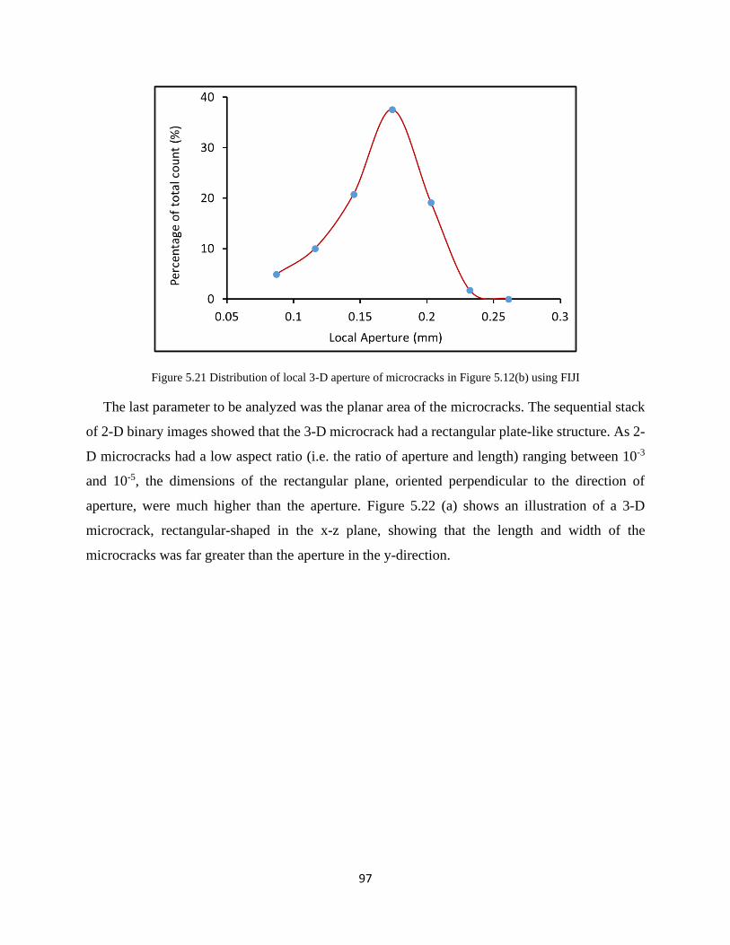
97
Figure 5.21 Distribution of local 3-D aperture of microcracks in Figure 5.12(b) using FIJI
The last parameter to be analyzed was the planar area of the microcracks. The sequential stack
of 2-D binary images showed that the 3-D microcrack had a rectangular plate-like structure. As 2-
D microcracks had a low aspect ratio (i.e. the ratio of aperture and length) ranging between 10-3
and 10-5, the dimensions of the rectangular plane, oriented perpendicular to the direction of
aperture, were much higher than the aperture. Figure 5.22 (a) shows an illustration of a 3-D
microcrack, rectangular-shaped in the x-z plane, showing that the length and width of the
microcracks was far greater than the aperture in the y-direction.

98
Figure 5.22 Pictorial representation of 3-D microcrack: (a) regenerated from 2-D binary images; (b) regenerated
from 2-D skeletonized binary images
As Section 5.3.1 stated, the process of 2-D skeletonization of a binary image converts a
microcrack with finite aperture into a single pixel-wide medial axis, always oriented perpendicular
to the direction of aperture of the microcrack. In Section 5.3.1, the macro in Appendix B (line no.
37) stored the skeletonized 2-D binary image in the separate skeleton directory. The skeletonized
2-D binary images were stacked and similar 3-D microcracks were regenerated with a unit 3-D
aperture. Figure 5.22 (b) shows an illustration of the skeletonized 3-D microcrack. A comparison
of 3-D microcrack in Figure 5.22 (a) and (b) shows that, except for the aperture in the y-direction,
both dimensions in the x- and z- directions were similar.
In FIJI, the plugin Isosurface of BoneJ (Lorensen & Cline, 1987) calculates the surface area of
a 3-D object that considers each of the three dimensions, such as the length, width and aperture of
the microcracks. However, there is no direct method in FIJI to calculate the area of only one plane
of a 3-D object. Therefore, in this study, an indirect method was improvised to calculate the area
of the plane of a 3-D microcrack. Since the volume of a 3-D object is the product of the sum of the
2-D area and the spacing between consecutive slices (Boudier, 2014), the area of a 3-D plane is
the product of sum of 2-D length of fractures and the spacing between the consecutive slices in z-

99
direction (Equation 5.3). Table 5.2 summarizes the results of the area of the plane of the
microcracks, shown in Figure 5.12(b). In addition, Appendix D presents the verification of the
rectangular-plate like structure of the 3-D microcracks.
A𝑟𝑒𝑎 𝑜𝑓 𝑝𝑙𝑎𝑛𝑒 = ∑ 𝑙𝑐𝑖
𝑛𝑖=1 ∗ 𝑍 𝑠𝑝𝑎𝑐𝑖𝑛𝑔 (5.3)
Similar to the 2-D geometry, the 3-D geometry of the microcracks was also determined using
Bruker CTAn. The plugin 3D Analysis analyzed the sequential stack of 2-D binary images and
calculated the volume and weighted-mean aperture of the microcracks. The plugin used the
Marching Cubes 33 algorithm (Chernyaev, 1995) to reconstruct the 3-D surface and calculate the
volume of the microcracks. Then, based upon the principle of local thickness (Dougherty and
Kunzelmann, 2007), the plugin 3D Analysis determined the weighted-mean value of local aperture
of microcracks. As Bruker CTAn does not calculate the 2-D skeletonized length of microcracks,
the plugin did not determine the area of the plane of the microcracks. Table 5.2 summarizes the
results of the calculation of the volume and aperture of the microcracks (shown in Figure 5.12),
and time taken for the analysis.
Table 5.2 Results of 3-D geometry of microcracks using FIJI and Bruker CTAn software
Geometrical
Parameter
FIJI Analysis Bruker CTAn
Analysis
Difference
(%)
Time (mins)
FIJI Bruker CTAn
3-D Volume (mm3) 536.30 533.8 0.5 0.5
8.1 3-D aperture (mm) 0.153 0.154 -0.65 37.8
Area of plane of
microcrack (mm2) 3,801.97 - - - -
Table 5.2 compares the results of the 3-D geometry of the microcracks and the time taken for
the analysis from FIJI and Bruker CTAn. The comparisons showed that the 3-D geometry was
approximately similar for both software, with a small percentage difference. However, the 3-D
geometrical analysis was computationally faster through Bruker CTAn when compared to FIJI.
Therefore, except for the area of the plane of the microcracks, this research calculated the 3-D
geometry of the microcracks using Bruker CTAn.

100
In addition to calculating the volume and aperture of microcracks using Bruker CTAn, the 3D
Analysis plugin also generated a new stack of 2-D binary images that contained information on the
local aperture of the microcracks. Solely for the purpose of 3-D visualization, the local aperture of
the microcracks was classified into three intervals, where each interval was represented by a
different color. Red represented the local aperture between 0.029 and 0.087 mm, green represented
the local aperture between 0.087 and 0.203 mm, and blue represented the local aperture between
0.203 and 0.319 mm. Figure 5.23 shows an illustration of this colored classification of the local
apertures of the microcracks.
Figure 5.23 3-D distribution of microcracks, where different colors represent different 3-D apertures of the
microcracks
5.4 Summary
This current section of research showed that X-ray CT is an effective technique for the non-
destructive visualization of the internal microstructure of shale. The North-Star Imaging M-5000
Industrial CT scanner showed microscopic features in the rock specimen up to a resolution of 29.7
microns. Both 2-D grayscale images and reconstructed 3-D images of the specimen provided
useful information on microcracks. The comparative analysis of several image-processing
techniques showed that the new proposed technique was useful in the image processing of the
poor-quality X-ray CT images. The macro, detailed in Appendix A, automated the image
101
processing and effectively generated the binary images of the microcracks. The macro, detailed in
Appendix B, automated the estimation of 2-D geometry and stored it in separate output directories,
while script (Appendix C) condensed the information into a single file. The comparison of the
results of the analysis of the 2-D and 3-D geometry of the microcracks showed that both FIJI and
Bruker CTAn were equally accurate. Although FIJI is an open source software with a slow speed
of computation, its capability for user-specific customization eased the estimation of the 2-D
geometry and planar area of the microcracks. The scatter plot between different 2-D geometrical
parameters against the individual slice position analyzed the distribution of microcracks. It was
found that the application of X-ray CT scanning and image processing was significantly useful in
the non-destructive quantification of microcracks in shale specimens.
102
Chapter 6 Assessment of the Geometry of Microcracks during Triaxial Creep
and Recovery Tests using the X-ray CT Scan Technique
In this chapter, the fundamental reason for creep deformation was investigated in bedded
Marcellus shale. First, this chapter describes the procedure for implementing laboratory creep and
recovery experiments combined with X-ray CT scanning of shale specimens. The next section
analyzes the results of the laboratory experiments in terms of time-dependent and time-
independent, elastic and plastic strains. The geometry of the specimen’s microcracks were
determined in 2-D and 3-D coordinate systems before and after the creep and recovery test. The
next section presents the comparison of plastic strains in shale specimens with the permanent
changes in the 3-D geometry of the microcracks. These comparisons provide useful insights on
the mechanism of creep deformation and the influence of extrinsic and intrinsic parameters on the
nature of creep deformation in the shale specimens.
6.1 Procedure for the triaxial creep and recovery test with X-ray CT scan
The ideal experimental setup to monitor the real-time changes in the geometry of microcracks
requires a dedicated X-ray CT equipment with a transparent triaxial chamber so that the
microcracks could be continuously monitored (Soldal, Wilkinson, Viken, & Sauvin, 2017; Liu,
Wang, & Zhang, 2018). However, based on the limitations of available technology, this study
adopted an alternative step-wise approach of loading and unloading the specimens and examining
the microcracks at different time steps of the laboratory experiments. This study included the
performance of two types of triaxial creep and recovery tests with X-ray CT scan. Each specimen
was a right cylindrical in shape, with both ends polished and ground flat to maintain the ends
parallel to 0.0013 mm. The ratio of length to diameter was greater than two (ASTM, 2019a). The
servo-controlled GCTS triaxial system (RTX-1500) applied conventional triaxial stress on the
specimen, such that the major principal stress (σ1) > intermediate (σ2) = minor principal stress (σ3).
The specimen remained sealed inside a Polyolefin jacket to prevent the contamination of the
confining oil and absorption of oil on the surface pores and cracks of the specimen. Axial and
lateral LVDTs, mounted onto the specimen, recorded the deformation in the axial and lateral
direction, respectively. A NorthStar Imaging M-5000 Industrial CT machine was used to scan each
specimen.

103
6.1.1 Type 1 triaxial creep and recovery test with X-ray CT scan
Figure 6.1 shows the experimental procedure for the Type 1 triaxial creep and recovery test
with X-ray CT scan. Eight Marcellus shale specimens were selected for the experiment that
included both parallel (PL) and perpendicular (PD) bedding to the orientation of the major
principal stress. In Figure 6.1, PD-29, PD-30, PD-31, and PD-37 were perpendicular-bedded
specimens, while PL-22, PL-23, PL-24, and PL-34 were parallel-bedded specimens. The X-ray
CT equipment scanned each of the eight specimens in the pre-test state. In the next step, each of
the four specimens with similar bedding orientations was maintained under constant triaxial stress
for successive time intervals. The procedure for the triaxial creep and recovery test involved four
stages, in addition to the hydrostatic consolidation of the specimen inside the RTX-1500. In the
hydrostatic consolidation stage, both axial and confining stress increased hydrostatically up to
1,000 psi. Afterwards, in stage 1, the axial stress increased to a predetermined value of differential
stress at the constant stress rate of 70 psi/second. In stage 2, the axial and confining stress remained
constant up to the predetermined time interval. In stage 3, the axial stress was lowered at the
constant rate of 70 psi/second until it reached the hydrostatic stress state of 1,000 psi. In stage 4,
the specimen was maintained at a hydrostatic stress state of 1,000 psi for at least 8 hours to monitor
the recovery of time-dependent elastic deformation. After finishing the triaxial experiment and
retrieving the intact core specimen, X-ray CT equipment scanned each specimen in the post-
triaxial stress state.
Figure 6.1 Experimental procedure for Type 1 triaxial creep and recovery test with X-ray CT scan

104
The objective of the Type 1 triaxial creep and recovery test was to analyze the influence of
bedding plane orientation and time intervals of constant stress on the creep behavior of the
Marcellus shale. This phenomenon was investigated through the application of similar levels of
constant differential stress on both types of bedded specimens for different time intervals. The
differential stress was equivalent to 70% of the failure strength at 1,000 psi confining pressure.
For example, among the perpendicular-bedded specimens, once the differential stress reached 70%
of the failure strength, PD-30 was unloaded immediately to the hydrostatic stress state. In contrast,
PD-31, PD-37, and PD-29 unloaded at successive longer time intervals. Similarly, among parallel-
bedded specimens, PL-23 unloaded immediately, while PL-24, PL-34, and PL-22 unloaded at
successive time intervals. In addition, monitoring of the strain recovery analyzed the immediate
and viscous deformation in shale. The X-ray CT imaging determined the geometry of microcracks
in the pre- and post- triaxial stress state.
6.1.2 Type 2 Triaxial Creep and Recovery Test with X-ray CT Scan
The objective of the Type 2 triaxial creep and recovery test with X-ray CT scan was to analyze
the influence of stress history, level of differential stress, and orientation of bedding plane on the
creep behavior of Marcellus shale. Figure 6.2 shows the experimental procedure for the Type 2
triaxial experiments. Four shale specimens of both parallel- and perpendicular-bedding orientation
were randomly selected for the experiment. The stress cycle 1 of loading and unloading the
bedded-shale specimen provided the stress history before the creep test in stress cycle 2. As Type
2 triaxial creep and recovery test involved the loading, unloading, and reloading of the specimen,
lower levels of differential stress was selected, such as 55% and 65% of failure strength at 1,000
psi confining pressure, in order to avoid the tertiary creep failure. For example, among the
perpendicular-bedded specimens, the experiment subjected PD-35 and PD-36 to an initial
differential stress equivalent to 55% and 65% of failure strength, respectively. Similarly, among
parallel-bedded specimens, the experiment subjected PL-32 and PL-33 to an initial differential
stress equivalent to 55% and 65% of failure strength, respectively

105
Figure 6.2 Experimental procedure for Type 2 triaxial creep and recovery test with X-ray CT scan
Each specimen was scanned before stress cycle 1 to determine the geometry of pre-existing
microcracks. In addition to the hydrostatic consolidation of the specimen at 1,000 psi, the test
procedure of stress cycle 1 involved two stages. In stage 1, the axial stress increased to the
predetermined value of differential stress at the constant stress rate increase of 70 psi/sec. In stage
2, the stress was immediately reduced to zero at the rate of 70 psi/sec. After the completion of
stress cycle 1, the specimens were retrieved from the triaxial cell and scanned using X-ray CT
equipment. In stress cycle 2, similar levels of differential stress was applied on each specimen,
which remained constant for four days. The test procedure of stress cycle 2 involved four stages.
In stage 1, the axial stress increased to the similar level of differential stress at the constant rate of
70 psi/second. In stage 2, the axial and confining stress remained constant for four days. In stage
3, the axial stress lowered at the stress rate of 70 psi/second to the hydrostatic stress of 1,000 psi.
In stage 4, the hydrostatic stress state remained constant for at least 8 hours to monitor the recovery
of time-dependent elastic deformations. Once stress cycle 2 finished, the specimens were scanned.
The X-ray CT scan at three different time steps determined the geometry of the microcracks in
pre, stress-cycle 1, post, stress-cycle 1, and post, stress-cycle 2 state.

106
6.2 Time-dependent strain in the rock subjected to constant stress state
Stress produces strain in rock. The nature of the strain depends on the level and nature of the
stress. For example, in the quasi-static loading condition, the differential stress increases at the
constant stress rate (72.5 – 145 psi/sec), or strain rate (10-5 – 10-3 per sec) (Zhang & Zhao, 2014),
and induces time-independent strain in the rock. Based on the level of differential stress, the time-
independent strain is a combination of elastic and plastic strain (Hobbs, 1970). After removing the
differential stress, some percentage of time-independent strain recovers, called the elastic strain;
the unrecovered strain in the specimen is called plastic strain (Mogi, 2006). Similarly, when
constant stress is applied on the rock for a long period of time, the induced strains are called time-
delayed or time-dependent strain, which may or may not recover completely upon the removal of
load. The time-delayed strain recovered with time upon the removal of load is called the elastic
time-strain (or viscoelastic strain), while the remaining fraction of time-delayed irrecoverable
strain is called the plastic time-strain (or viscoplastic strain) (Evans, 1936).
As shown in Figure 6.3, the creep and recovery test on concrete broke the cumulative time-
dependent creep strain into recoverable, delayed elastic strain and irrecoverable flow (Illston,
1978). Kim et al. (2009) modeled the permanent deformation in Hot Mixture Asphalt (HMA)
through the estimation of viscoplastic strain from creep and recovery tests. This study showed that
the measured time-delayed strain in creep and recovery tests allowed for the easy separation of
viscoelastic and viscoplastic strain components, as shown in Figure 6.4. Similarly, Sone (2012)
determined the viscoplastic creep deformation with the slight viscoelastic component during cyclic
creep and recovery tests on Haynesville-dark shale. The cyclic-loading and unloading method also
determined the recoverable elastic and viscoelastic strain and irrecoverable plastic and viscoplastic
strain in the composite layered specimens (Hu, Yang, Xu, & Cheng , 2019). Therefore, the creep
and recovery tests can break down the cumulative strain into elastic, plastic, viscoelastic, and
viscoplastic strains.

107
Figure 6.3 Time dependent creep deformation of concrete (Mehta & Monteiro, 2006)
Figure 6.4 Decomposition of time-dependent strain in HMA from creep and recovery testing (Kim et al., 2009)
Figure 6.5 shows the idealized curve between differential stress and time during the creep test,
subdivided into four regions that represent the accumulation and recovery of different types of
strain in the specimen. In region 1, from zero to time step 1, the differential stress increased from
zero to the predetermined level and the instantaneous strain was a combination of elastic and
plastic strain. Once the differential stress became constant, the strain accumulated between time
step 1 and time step 2 was a combination of viscoelastic and viscoplastic strain. After the end of
the constant stress state, between time step 2 and time step 3, the differential stress reduced at the

108
constant rate, and the amount of strain recovered upon unloading was elastic strain. At the zero-
differential stress from time step 3 to time step 4, the recovered strain was viscoelastic in nature.
Therefore, at the end of the triaxial creep and recovery test, the unrecovered strain in the specimen
was a combination of plastic and viscoplastic strain. As the data acquisition unit of servo-
controlled GCTS – triaxial system continuously captured the total strain in the specimen, the
mathematical relationship in equation 6.1 breaks down the total strain into its components.
Equation 6.1 represents the total strain in either direction at time step 1, time step 2, time step 3,
and time step 4 as 𝜀𝑇1, 𝜀𝑇2, 𝜀𝑇3 , and 𝜀𝑇4, respectively. In addition, Equation 6.1 represents the
elastic, plastic, viscoelastic, and viscoplastic strain as: 𝜀𝑒, 𝜀𝑝, 𝜀𝑣𝑒 , and 𝜀𝑣𝑝, respectively.
Figure 6.5 Disintegration of differential stress versus time curve into different regions based on the nature of
differential stress
𝜀𝑒 + 𝜀𝑝 = 𝜀𝑇1
𝜀𝑣𝑒 + 𝜀𝑣𝑝 = 𝜀𝑇2 − 𝜀𝑇1
𝜀𝑒 = 𝜀𝑇2 − 𝜀𝑇3
𝜀𝑣𝑒 = 𝜀𝑇3 − 𝜀𝑇4 (6.1)
6.3 Results of the triaxial creep and recovery test with X-ray CT scan
This section contains four subsections, individually explaining the experimental results of the
two different types of triaxial creep and recovery tests, as well as the geometry of the microcracks
before and after the completion of Type 1 and Type 2 experiments.
109
6.3.1 Results of Type 1 triaxial creep and recovery test on bedded Marcellus shale
The average failure strengths of parallel- and perpendicular-bedded specimens in axial
direction, confined at 1,000 psi pressure, were 19,691 psi and 18,162.7 psi, respectively. In Type
1 triaxial creep and recovery tests, both types of shale specimens were subjected to constant
differential stress equivalent to 70% of the failure strength at 1,000 psi confining pressure. Figure
6.6 shows the axial stress versus strain curve for each specimen during the Type 1 experiment.
Figure 6.7 shows the creep strain versus time curve of each specimen. Both figures show the four
different stages of the triaxial creep and recovery test; stage 1 represented the increase in axial
stress, stage 2 represented the constant axial stress, stage 3 represented the decrease in the axial
stress, and stage 4 represented the hydrostatic stress of 1,000 psi. A malfunction in data acquisition
occurred where it did not record the data for stage 3 in specimen PD-30. The figures provided the
following information:
• At constant differential stress, the creep deformation of the shale specimens did not increase
steadily with time. Although the axial and lateral LVDTs were calibrated before the creep
experiments, the creep strain fluctuated with time.
• The perpendicular-bedded specimens, PD-31 and PD-29, only experienced creep deformation
in the axial direction.
• Specimen PD-37 exhibited elastic behavior. As shown in Figure 6.6, the axial stress versus
strain curve coincided in the loading and unloading conditions. In addition, specimen PD-37
experienced strain recovery in the axial and radial directions at the constant stress state.
• Parallel-bedded specimens, PL-22 and PL-24 entered the tertiary stage of creep deformation
due to the exponential increase in radial strain. However, at a similar level of constant stress,
specimen PL-34 experienced strain recovery in the radial direction. The uniaxial creep test on
Warsop nodular, muddy limestone by Price (1964) showed similar behavior of a decrease in
creep strain at a high constant stress (Figure 2.7). According to Price, the behavior
corresponded to the release of residual strain energy from the specimens.
• In the hydrostatic stress state of 1,000 psi, specimens PD-31, PD-29, PL-22, and PL-24 showed
viscoelastic strain recovery.

110
Figure 6.6 Axial stress versus strain curves for Type 1 triaxial creep and recovery tests

111
Figure 6.7 Strain versus time curve for Type 1 triaxial creep and recovery test

112
Table 6.1 summarizes the experimental results of the Type 1 experiment, including the value
of axial stress, duration of constant stress state, rate of secondary creep strain, modulus of
elasticity, and Poisson’s ratio. Through the ASTM recommended secant method (ASTM, 2014),
the modulus of elasticity was determined using the axial stress versus axial strain curve between
zero and an axial stress equivalent to 40% of the failure strength. The results showed that, although
the triaxial stress path was the same, the secant modulus of elasticity and Poisson’s ratio were
significantly different among the parallel- and perpendicular-bedded specimens. The rate of
secondary creep strain in the axial and radial direction was very small, indicating the slow
deformation of brittle shale specimens. The negative and positive value of axial and radial rate of
secondary creep strain, respectively, also indicated that specimen PD-37, PL-34 experienced strain
recovery. Specimen PL-24 also exhibited small strain recovery in axial direction before it entered
the tertiary stage of creep deformation under radial dilation.
Table 6.1 Results of the Type 1 experiment on bedded Marcellus shale
Specimen
ID
Specimen
type
Confining
stress
(psi)
Axial
stress
(psi)
Duration of
constant
stress state
(hours)
Rate of secondary
creep strain
(%/hours)
Secant
modulus of
elasticity
(KPsi)
Poisson’s
ratio
Axial Radial
PD-30
Perpendicular
1,000
12,713.89
0 - - 18,318 0.09
PD-31 208.78 1E-06 -3E-07 10,552.53 0.003
PD-37 360 -1E-07 1E-07 9,896.86 0.02
PD-29 746.77 2E-08 1E-08 9,464.85 0.006
PL-23
Parallel
1,000
13,783.7
0 - - 21,708.17 0.05
PL-24 128.18 1E-06 -2E-07 9,306.91 0.02
PL-34 192 -3E-07 9E-07 9,773.12 0.12
PL-22 283.42 -4E-07 -4E-08 20,679.19 0.03
Based on Equation 6.1, the total strain was broken down into elastic, plastic, viscoelastic, and
viscoplastic strain. Table 6.2 summarizes the different types of strains in each specimen. The
results showed that, although the maximum axial stress and rate of increase in axial stress was the
same, the elastic and plastic strain was significantly different between parallel-and perpendicular-

113
bedded specimens. The perpendicular-bedded specimens experienced significantly small strain in
radial direction compared to parallel-bedded specimens. Figure 6.8 shows the comparison of creep
strain, i.e. the arithmetic sum of viscoelastic and viscoplastic strain, with time under constant stress
state for parallel- and perpendicular-bedded specimens. The results showed that, at similar constant
stresses, the creep strain in either direction did not always increase with time in both parallel- and
perpendicular-bedded specimens. It also showed that, although the duration of constant stress on
parallel-bedded specimens was smaller compared to perpendicular-bedded specimens, parallel-
bedded specimen experienced significantly higher radial and axial creep strain compared to
perpendicular-bedded specimens.
Table 6.2 Different types of strain in shale specimen during Type 1 triaxial creep and recovery test
Specimen
ID
Elastic
strain (%)
Viscoelastic
strain (%)
Plastic
strain (%)
Viscoplastic
strain (%)
Axial Radial Axial Radial Axial Radial Axial Radial
PD-30 0.0537 -0.0102 - - 0.0414 -0.004 - -
PD-31 0.1436 -0.0044 0.0003 0.00 0.0007 0.00 0.0184 0.00
PD-37 0.1189 -0.0046 0.0025 -0.01 0.00 0.00 0.00 0.00
PD-29 0.1004 -0.023 0.0007 0.00 0.0344 0.00 0.0285 0.00
PL-23 0.0561 -0.0277 - - 0.023 0.00 - -
PL-24 0.1123 -0.063 0.018 -0.0186 0.0302 0.00 0.0223 -0.0578
PL-34 0.0984 -0.0244 0.0073 -0.0066 0.0324 0.00 0.00 0.00
PL-22 0.0866 -0.0581 0.0081 -0.0077 0.0561 -0.0325 0.00 -0.2545

114
Figure 6.8 The comparison between creep strain versus time under constant stress for parallel- (PL) and
perpendicular- (PD) bedded shale specimens
Therefore, the type 1 triaxial creep and recovery test showed that the shale specimens exhibited
heterogeneous deformation in terms of instantaneous strain, modulus of stiffness and Poisson’s
ratio. The constant stress caused both viscoelastic and viscoplastic creep deformation. However,
the creep strain did not always increase with time at similar differential stress. The orientation of
bedding plane influenced the nature of the creep deformation in the shale specimens, such that
parallel-bedded specimens experienced higher radial deformation as compared to perpendicular-
bedded specimens.
6.3.2 Results of Type 2 triaxial creep and recovery test on bedded Marcellus shale
In the Type 2 triaxial experiments, two specimens of parallel- and perpendicular- bedding
orientation were subjected to two successive levels of differential stress. The stress was applied in
two successive stress cycles. In stress cycle 1, the axial stress increased up to the predetermined
level and immediately unloaded to the zero-stress state. In stress cycle 2, the axial stress increased
up to a similar level and remained constant for four days. Figure 6.9 shows the axial stress versus
strain curve for each specimen in stress cycle 1 and stress cycle 2, while Figure 6.10 shows the
strain and time curve for each specimen in stress cycle 1 and stress cycle 2. In the legends of both
figures, Stage 1_Cycle 1 and Stage 3_Cycle 1 represent the increase and decrease in axial stress
during stress cycle 1, respectively; similarly, Stage 1_Cycle 2 and Stage 3_Cycle 2 represent the
increase and decrease in the axial stress during stress cycle 2, respectively. In addition, Stage

115
2_Cycle 2 and Stage 4_Cycle 2 represents the constant state of axial stress equivalent to either
55% or 65% of failure strength and hydrostatic stress state of 1,000 psi, respectively. As the overall
duration of stress cycle 1 was much less than the duration of stress cycle 2, Stage 1_Cycle 1 and
Stage 3_Cycle 1 are not visible in Figure 6.10. The Figures provided the following useful
information:
• In specimen PD-35, the axial stress versus strain curve in Stage 1_Cycle 1 and Stage 3_Cycle
1 coincided with one another thereby indicating the elastic behavior of PD-35 in stress cycle 1.
The axial stress versus strain curve in Stage 1_Cycle 2 lies to the right of the Stage 1_Cycle 1;
this implies that the instantaneous strain in PD-35 was higher in stress cycle 2 than in stress
cycle 1. In stress cycle 2, the constant stress caused significant creep deformation in the axial
direction and axial strain recovery in the hydrostatic stress state. However, the specimen did not
experience significant creep deformation in the radial direction.
• In specimen PD-36, the instantaneous strain during stress cycle 1 and stress cycle 2 were quite
close to one another, such that stress cycle 2 induced smaller instantaneous strain compared to
stress cycle 1. In stress cycle 2, the constant stress caused creep deformation in the axial
direction during loading and axial strain recovery in the hydrostatic stress state. However,
similar to PD-37 and PL-34, PD-36 experienced radial strain recovery under the high constant
stress state.
• In specimen PL-32, stress cycle 2 induced higher instantaneous strain compared to stress cycle
1. The specimen also experienced significant permanent compression in the axial direction at
the end of stress cycle 1. In stress cycle 2, the constant stress did not cause creep deformation
in the axial or the radial directions; rather, the specimen showed radial strain recovery at high
constant stress state.
• In specimen PL-33, although the initial axial stress vs axial strain curve initially coincided
during Stage 1_Cycle 1 and Stage 1_Cycle 2, stress cycle 2 induced higher instantaneous axial
strain compared to stress cycle 1. In stress cycle 2, the constant stress caused creep deformation
in the axial direction and small strain recovery in the hydrostatic stress state. However, the
specimen did not experience creep deformation in the radial direction.

116
Figure 6.9 Axial Stress versus Strain curve for Type 2 Triaxial Creep and Recovery Test
Figure 6.10 Strain versus Time curve for Type 2 Triaxial Creep and Recovery Test

117
Table 6.3 summarizes the experimental results of the Type 2 triaxial creep and recovery test,
including axial stress, duration of constant stress state, rate of secondary creep strain in axial and
radial directions, modulus of elasticity, and Poisson’s ratio. Similar to the Type 1 triaxial
experiment, secant method determined the modulus of elasticity in the Type 2 triaxial experiments.
The results of rate of secondary creep strain showed that, under high constant differential stress,
specimen PD-36 and PL-32 experienced strain recovery at high constant differential stress. The
results also showed that the secant modulus of elasticity and Poisson’s ratio changed from stress
cycle 1 to stress cycle 2. The stress history of stress cycle 1 decreased the modulus of stiffness and
increased the Poisson’s ratio.
Table 6.3 Results of Type 2 triaxial creep and recovery test on bedded Marcellus Shale
Specimen
ID
Confining
stress
(psi)
Axial
stress
(psi)
Stress
cycle
Duration of
constant
stress state
(hours)
Rate of secondary creep
strain
Secant
modulus of
elasticity
(KPsi)
Poisson’s
ratio
Axial
(%/hours)
Radial
(%/hours)
PD-35
1,000
9,989
Cycle 1 0 - - 24,042.02 0.03
Cycle 2 96 4E-06 -2E-07 18,228.96 0.5
PD-36
11,805
Cycle 1 0 - - 10,351.81 0.05
Cycle 2 96 -3E-07 3E-06 10,861.57 0.29
PL-32
1,000
10,830
Cycle 1 0 - - 14,011.54 0.02
Cycle 2 96 -2E-07 9E-07 10,000.71 0.19
PL-33
12,799
Cycle 1 0 - - 10,478.69 0.25
Cycle 2 96 6E-07 4E-07 10,977.37 0.25
We also compared the elastic and plastic component of the instantaneous strain between stress
cycle 1 and stress cycle 2; Table 6.4 summarized these results. Except for specimen PL-32, the
stress cycle 1 only caused elastic deformation in each specimen with insignificantly small plastic
component. The instantaneous strain increased from stress cycle 1 to stress cycle 2. However,
except for PL-32, the plastic component of instantaneous strain increased in axial direction, while
decreased in radial direction from stress cycle 1 to stress cycle 2.

118
Table 6.4 Comparison of elastic and plastic components of axial and radial strain between stress cycle 1 and cycle 2
Specimen
ID
Stress
cycle
Axial direction
Radial direction
Change in
instantaneous strain
from stress cycle 1 to
cycle 2 (%)
Instanta
neous
strain
(%)
Elastic
component
(%)
Plastic
component
(%)
Instanta
neous
strain
(%)
Elastic
component
(%)
Plastic
component
(%)
Axial
direction
Radial
direction
PD-35
Cycle 1 0.0418 98.80 1.20 -0.0021 95.24 4.76
58.85
323.81 Cycle 2 0.0664 57.08 42.92 -0.0089 100 0
PD-36
Cycle 1 0.11 99.91 0.09 -0.0043 0 100
-7.82
-67.44 Cycle 2 0.104 92.70 7.30 -0.0014 100 0
PL-32
Cycle 1 0.0853 80.07 19.93 -0.006 98.33 1.67
21.10
121.67 Cycle 2 0.1033 96.22 3.78 -0.0133 100 0
PL-33
Cycle 1 0.109 99.08 0.92 -0.0328 93.29 6.71
8.35
-16.77 Cycle 2 0.1181 95.77 4.23 -0.0273 100 0
During cyclic tests, the increase in instantaneous strain at loading and permanent strain at
unloading is the characteristic of damage accumulation in hard rock specimens (Haimson, 1978).
In addition, the increase in Poisson’s ratio and decrease in modulus of stiffness in successive stress
cycles was indicative towards the progressive growth of damage in rock sample during loading
cycles (Taheri, Hamzah, & Dai, 2017). These results showed that the hard shale significantly
weakened due to cyclic loading condition. However, the behavior of cyclic deformation was
different than other brittle rocks. According to Haimson (1978), hard rocks like Tennessee marble
and Berea sandstone experienced the highest plastic strain in the first cycle of cyclic test, as much
as 30 to 70 percent of total plastic strain just before failure. The cyclic axial load was between 70
to 95 percent of uniaxial compressive strength. These current experiments had the axial stress
unloading at 55 and 65 percent of failure strength that primarily caused elastic strain in first stress
cycle in both types of bedded specimens. However, in the second stress cycle, overall axial strain
and its plastic component increased in specimen PD-35, PD-36 and PL-33; this implies that cyclic
loading at small stress (55-65% of failure strength) weakened the hard rock through continued

119
accumulation of higher plastic deformation. In addition, it was inferred that the higher plastic
deformation in the second stress cycle also contributed to the creep deformation.
Based on Equation 6.1, the total strain was disintegrated into elastic, plastic, viscoelastic, and
viscoplastic strain. Table 6.5 summarizes these results and shows that, in both types of bedded
specimens, constant stress caused both viscoelastic and viscoplastic creep strain in axial direction.
However, in radial direction, each specimen only experienced viscoelastic strain recovery and zero
viscoplastic strain. Figure 6.11 shows the comparison of cumulative creep strain in axial direction
with the level of differential stress. These results showed that, although the differential stress
increased from 55% to 65%, the axial creep strain decreased significantly in perpendicular-bedded
specimens. However, in parallel-bedded specimens, the axial creep strain increased with the
differential stress.
Table 6.5 Different types of strain in shale specimen during Type 2 triaxial creep and recovery test
Specimen
ID
Stress
cycle
Elastic strain (%) Viscoelastic strain (%) Plastic strain (%) Viscoplastic strain (%)
Axial Radial Axial Radial Axial Radial Axial Radial
PD-35
Cycle 1 0.0413 -0.002 - - 0.0005 -0.0001 - -
Cycle 2 0.0379 -0.0089 0.0031 -0.0066 0.0285 0.00 0.0422 0.00
PD-36
Cycle 1 0.1099 0 - - 0.0001 -0.0043 - -
Cycle 2 0.094 -0.0014 0.0033 -0.027 0.0074 0.00 0.0062 0.00
PL-32
Cycle 1 0.0683 -0.0059 - - 0.017 -0.0001 - -
Cycle 2 0.0994 -0.0133 0.0016 -0.0093 0.0039 0.00 0.00 0.00
PL-33
Cycle 1 0.108 -0.0306 - - 0.001 -0.0022 - -
Cycle 2 0.1131 -0.0273 0.0005 -0.0029 0.005 0.00 0.0127 0.00

120
Figure 6.11 The comparison of axial creep strain with the level of differential stress in Type 2 creep and recovery
experiment
Therefore, the type 2 triaxial creep and recovery test showed that the stress history weakened
the hard shale specimens. The constant stress caused both viscoelastic and viscoplastic creep
deformation of shale specimens. However, the increase in differential stress did not always
increase the creep strain in shale specimens. The orientation of bedding plane did not influence the
nature of creep deformation in shale specimens.
6.3.3 Change in geometry of microcracks during Type 1 triaxial creep and recovery test
The X-ray CT equipment scanned cylindrical shale specimens and generated two-dimensional
grayscale images; next, by sequentially stacking the two-dimensional images, it reconstructed a
three-dimensional image of the specimen. Both types of X-ray CT images yielded different types
of geometric parameters, categorized as two- and three- dimensional geometry of microcracks.
The two-dimensional (2-D) geometry of microcracks included area, weighted-mean aperture,
and length of microcracks. As explained in the previous chapter, FIJI was used to determine the 2-
D geometry of microcracks. The three-dimensional geometry of microcracks included the volume,
weighted-mean aperture, and area of plane of microcracks. Bruker CTAn and FIJI determined the
different 3-D geometric parameters. Specimens of the Type 1 triaxial experiment were scanned in
both the pre- and post- triaxial test states; next, we analyzed the stress-induced changes in the 2-D
and 3-D geometry of microcracks through the comparison of average value of cumulative area (ac)
and the volume of microcracks in the pre- and post-triaxial stress states. Table 6.6 summarizes
these results.

121
Table 6.6 Comparison of 2-D area and 3-D volume of microcracks tested in Type 1 triaxial experiment
Specimen
ID
Average 2-D microcrack
area (mm2)
3-D microcrack volume
(mm3) Stress induced difference (%)
Pre-stress Post-stress Pre-stress Post-stress Average 2-D area 3-D volume
PD-30 7.08 11.21 771.5 1,186.9 58.29 53.85
PD-31 4.7 5.87 507.36 617.24 24.9 21.66
PD-37 2.36 1.56 232.86 148.24 -33.81 -36.34
PD-29 4.31 7.11 472.17 764.09 65.08 61.83
PL-23 8.62 9.7 936.22 1,063.29 12.54 13.57
PL-24 2.76 17.2 294.93 1,883.8 524.25 538.72
PL-34 1.27 6.05 123.74 618.19 377.85 399.57
PL-22 7.46 41.11 803.75 4,521.66 451.41 462.57
The results in Table 6.6 showed that each specimen had a significant amount of microcracks in
the pre-stress state, which was considered to be pre-existing microcracks. The 2-D area and 3-D
volume of microcracks were different for each specimen in the pre-triaxial stress state, indicating
towards the non-homogeneity of specimens cored from similar locations. The results in the column
of stress induced difference in Table 6.6 indicated that the constant triaxial stress, equivalent to
70% of the failure strength, caused significant changes in the 2-D area and 3-D volume of pre-
existing microcracks. Except for specimen PD-37, each specimen exhibited an increase in the area
and volume of pre-existing microcracks. The higher value of area and volume of microcracks in
the post-triaxial stress state could be due to the propagation of pre-existing microcracks and/or the
nucleation of new microcracks. Figure 6.12 shows the comparison between stress induced
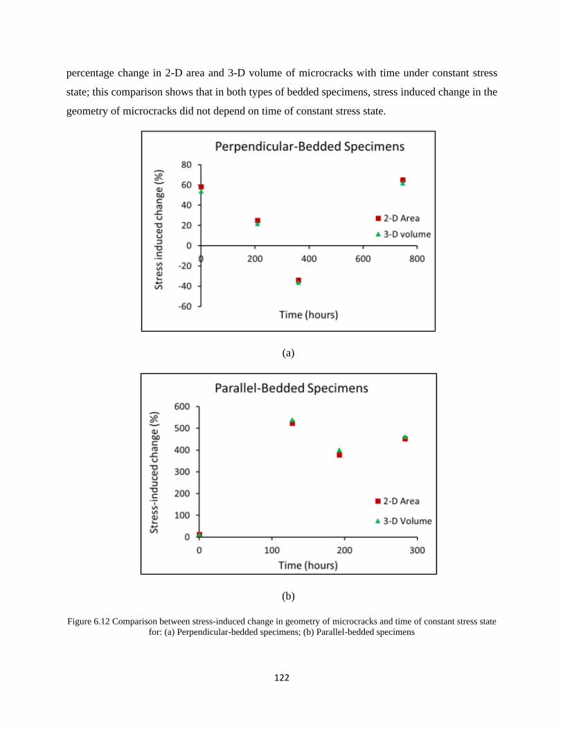
122
percentage change in 2-D area and 3-D volume of microcracks with time under constant stress
state; this comparison shows that in both types of bedded specimens, stress induced change in the
geometry of microcracks did not depend on time of constant stress state.
(a)
(b)
Figure 6.12 Comparison between stress-induced change in geometry of microcracks and time of constant stress state
for: (a) Perpendicular-bedded specimens; (b) Parallel-bedded specimens
123
The mode of increase in 2-D area of microcracks was analyzed through the comparison of
weighted-mean aperture and the 2-D length of microcracks in the pre- and post-triaxial stress
states; the mode of increase in 3-D volume of microcracks was analyzed through the comparison
of weighted-mean aperture and area of plane of microcracks in the pre- and post-triaxial stress
states. Table 6.7 summarizes these results. The stress induced percentage change in the respective
parameters showed that mode of increase in the 2-D area and the 3-D volume of microcracks was
a characteristic of the specimen’s bedding plane orientation with respect to the direction of major
principal stress. Except for specimen PD-37, each perpendicular-bedded specimen, such as PD-
30, PD-31, and PD-29 experienced a significant increase in the 2-D length and the 3-D area of
microcrack plane, whereas the 2-D and 3-D weighted-mean aperture either decreased or increased
non-significantly to contribute towards the increase in area or volume of microcracks. However,
the parallel-bedded specimens, such as PL-23, PL-24, PL-34, and PL-22 experienced a significant
increase in both aperture and length of microcracks in both 2-D and 3-D; this result implied that,
in perpendicular-bedded specimens, either the pre-existing microcracks propagated or new
microcracks nucleated with significantly small aperture compared to parallel-bedded specimens.
As the test stressed each specimen at similar levels of triaxial stress with respect to the failure
strength, the orientation of bedding plane influenced the direction of microcrack propagation.

124
Table 6.7 Comparison of 2-D and 3-D geometrical parameters to analyze the mode of change in area and volume of microcracks in Type 1 triaxial experiment
Specimen
ID
Average of 2-D
weighted-mean
aperture (mm)
Average of
cumulative 2-D
length (mm)
3-D weighted-
mean aperture
(mm)
3-D area of plane of
microcracks (mm2) Stress-induced change (%)
Pre -
stress
Post -
stress
Pre -
stress
Post -
stress
Pre -
stress
Post -
stress
Pre -
stress
Post -
stress
2-D
aperture 2-D length
3-D
aperture
3-D area of
microcrack plane
PD-30 0.114 0.109 52.05 78.76 0.136 0.135 5,859.09 9,046.73 -3.44 51.32 -0.95 54.4
PD-31 0.089 0.087 35.69 46.81 0.125 0.124 4,052.42 5,196.51 -3.48 31.16 -0.86 28.23
PD-37 0.067 0.055 15.9 10.31 0.129 0.094 1,708.38
1,119.43
-18.44 -35.16 -26.65 -34.47
PD-29 0.076 0.078 32.02 56.45 0.124 0.129 3,665.59 6,381.84 1.89 76.31 4.19 74.10
PL-23 0.107 0.119 68.04 63.45 0.138 0.160 7,619.83 7,487.84 12.14 -6.75 16.24 -1.73
PL-24 0.081 0.114 22.49 116.18 0.115 0.166 2,553.07 13,131.33 39.89 416.55 44.57 414.34
PL-34 0.076 0.101 9.83 37.99 0.106 0.145 1,072.38 4,201.41 32.37 286.5 37.21 291.78
PL-22 0.094 0.149 59.01 234.51 0.125 0.204 6,614.32 26,505.35 58.63 297.4 63.28 300.73

125
Figure 6.13 shows the graph between the cumulative area of microcracks and the individual
slice position in pre-stress state, displaying the distribution of pre-existing microcracks along the
length of specimens. In addition, the similar graphs in the post- triaxial stress state indicate the
stress-affected regions along the specimen length. Here, first and last individual slice position
represented the two different end surfaces of the specimen, in contact with the top and bottom
platen of the triaxial apparatus, respectively. The zero value of cumulative 2-D area at either end
was due to the limitation of X-ray CT equipment in imaging the end surfaces. In the pre-stress
state, the value of cumulative 2-D area was always higher at either ends; implies that the possible
reason for this higher area of microcracks at both ends could be the coring and dry cutting of shale
specimens. The figure also shows that, for specimens PL-23, PD-31, and PD-37, the overall
distribution of cumulative 2-D area of microcracks was coherent in the pre- and post- triaxial stress
states; this indicates the uniform propagation or contraction of pre-existing microcracks. However,
in specimens PD-29, PD-30, PL-22, PL-24, and PL-34, the cumulative 2-D area of microcracks
exponentially increased in the post- triaxial stress state compared to the pre-triaxial stress state;
this indicates the formation of a new plane of microcracks in the specimens. The graph also shows
the region of maximum damage intensity due to larger areas of microcracks. For example, except
for either end, the cumulative area of microcracks was highest at half of the specimen’s length in
specimens PD-30 and PD-29.

126
Figure 6.13 The graph between cumulative 2-D area of microcracks and individual slice position in pre- and post-
stress state for Type 1 triaxial creep and recovery test
127
The visual comparison of microcracks between pre- and post-triaxial stress state allowed the
evaluation of the propagation of pre-existing microcracks or formation of new plane of
microcracks. Two methods were used to visualize the microcracks. The first method was a
comparison of the vertical projection of all 2-D microcracks on a two-dimensional plane; Figure
6.14 shows these results. Except for specimens PD-31and PD-37, triaxial stress generated a new
plane of microcracks (enclosed in a red boundary in post-stress state) in each specimen. The high
intensity of new planes of microcracks in specimens PD-29, PD-30, PL-22, PL-24, and PL-34
supported the exponential increase in cumulative 2-D area of microcracks in Figure 6.13. In PD-
31, the average value of cumulative 2-D area of microcracks increased by 24.9% that indicates the
significant propagation of pre-existing microcracks under triaxial stress. In PD-37, triaxial stress
closed the pre-existing microcracks.
The second method was a visual comparison of 3-D distribution of microcracks in the pre- and
post-triaxial stress states. As shown in Figure 6.15, specimens PD-29 and PD-30 exhibited the
formation of a new plane of microcracks, parallel to the direction of major principal stress.
However, the density of pre-existing microcracks in specimen PD-31 increased in the post-stress
state compared to the pre-stress state; this indicates that the propagation of pre-existing
microcracks contributed towards the increase in the total volume of microcracks by 21.66% (Table
6.6). In specimem PD-37, the density of pre-existing microcracks decreased in the post-stress state
compared to the pre-stress state that indicates the contraction of microcracks and the decrease in
total volume of microcracks by 36.34%. In Figure 6.16, specimens PL-24, PL-34, and PL-22
exhibited the formation of a new plane of microcracks, parallel to the direction of major principal
stress and contraction of the few pre-existing microcracks. In specimen PL-23, the density of the
pre-existing plane of microcracks increased and few of pre-existing microcracks on the edges
closed in the post-stress state compared to pre-stress state; this indicates that the applied triaxial
stress caused both propagation and contraction of pre-existing microcracks.

128
Figure 6.14 Vertical projection of 2-D microcracks in pre- and post-stress state in Type 1 triaxial creep and recovery
test

129
Figure 6.15 Three-dimensional comparison of microcracks in pre-and post-stress state in perpendicular specimens of Type 1 triaxial creep and recovery test

130
Figure 6.16 Three-dimensional comparison of microcracks in pre-and post-stress state in parallel specimens of Type 1 triaxial creep and recovery test

131
Therefore, the X-ray CT scan of shale showed that each specimen was heterogenous with
varying density of pre-existing microcracks. The applied triaxial stress not only propagated and
contracted the pre-existing microcracks, but also formed a new plane of microcracks parallel to
the direction of major principal stress in both types of bedded specimens. The orientation of
bedding plane influenced the mode of increase in 2-D area and 3-D volume of microcracks.
However, time under constant stress state did not influence the stress-induced change in the
geometry of microcracks.
6.3.4 Change in geometry of microcracks during Type 2 triaxial creep and recovery test
In Type 2 experiment, the X-ray CT equipment scanned the specimen at three different time steps:
pre-stress cycle 1, post-stress cycle 1, and post-stress cycle 2. As explained previously, the X-ray
CT equipment first generated 2-D grayscale images of the specimen, and a 3-D image was
reconstructed from the sequential stacking of 2-D images. Therefore, this study determined the
geometry of microcracks in both 2-D and 3-D coordinate systems. The comparison of the average
value of cumulative 2-D area and 3-D volume of microcracks analyzed the changes in the geometry
of microcracks due to stress cycle 1 and stress cycle 2. Table 6.8 summarizes these results.
Table 6.8 Comparison of 2-D area and 3-D volume of microcracks in Type 2 triaxial creep and recovery test
Specimen
ID
Average 2-D
microcrack area (mm2)
3-D microcrack
volume (mm3)
Stress-induced change
between post-cycle 1
and pre-stress (%)
Stress-induced change
between post-cycle 2
and post-cycle 1 (%)
Pre-
stress
Post-
cycle 1
Post-
cycle 2
Pre-
stress
Post-
cycle 1
Post-
cycle 2
Average
2-D area
3-D
volume
Average
2-D area
3-D
volume
PD-35 2.23 1.65 2.55 231.71 166.04 260.25 -26.28 -28.34 54.96 56.74
PD-36 3.16 2.36 2.78 330.04 240.46 282.42 -25.44 -27.14 17.71 17.45
PL-32 1.81 0.38 0.98 185.24 36.58 96.77 -78.98 -80.25 158.95 164.57
PL-33 2.03 1.17 1.75 208.95 117.85 177.45 -42.34 -43.59 49.31 50.58
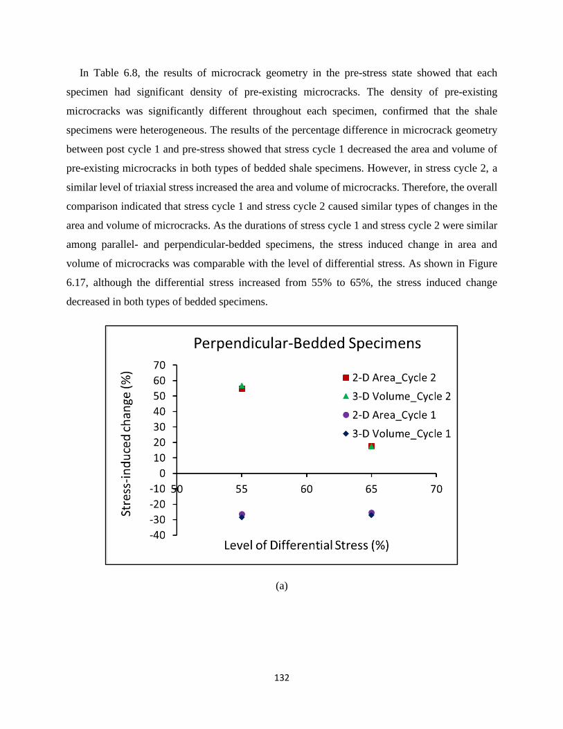
132
In Table 6.8, the results of microcrack geometry in the pre-stress state showed that each
specimen had significant density of pre-existing microcracks. The density of pre-existing
microcracks was significantly different throughout each specimen, confirmed that the shale
specimens were heterogeneous. The results of the percentage difference in microcrack geometry
between post cycle 1 and pre-stress showed that stress cycle 1 decreased the area and volume of
pre-existing microcracks in both types of bedded shale specimens. However, in stress cycle 2, a
similar level of triaxial stress increased the area and volume of microcracks. Therefore, the overall
comparison indicated that stress cycle 1 and stress cycle 2 caused similar types of changes in the
area and volume of microcracks. As the durations of stress cycle 1 and stress cycle 2 were similar
among parallel- and perpendicular-bedded specimens, the stress induced change in area and
volume of microcracks was comparable with the level of differential stress. As shown in Figure
6.17, although the differential stress increased from 55% to 65%, the stress induced change
decreased in both types of bedded specimens.
(a)

133
(b)
Figure 6.17 The comparison between stress induced change in area and volume of microcracks with level of
differential stress for: (a) Perpendicular-bedded specimens; (b) Parallel-bedded specimens.
Like the Type 1 experiment, the mode of change in area and volume of microcracks was
determined during stress cycle 1 and stress cycle 2. In 2-D, Table 6.9 summarizes the comparison
in average value of weighted-mean aperture and cumulative 2-D length of microcracks at three-
different time steps. The results show that stress cycle 1 reduced both the 2-D aperture and length
of microcracks in parallel- and perpendicular-bedded specimens. However, stress cycle 2 increased
the length and decreased the aperture of microcracks in both types of bedded specimens. In 3-D,
Table 6.10 summarizes the comparison between 3-D weighted-mean aperture and area of plane of
microcracks. The results show that stress cycle 1 reduced both the 3-D aperture and area of plane
of microcracks in parallel- and perpendicular-bedded specimens. However, stress cycle 2 increased
the area of plane of microcracks and decreased the 3-D aperture of microcracks in both types of
bedded specimens. The overall comparison indicates that the stress history of stress cycle 1 closed
the pre-existing microcracks, while stress cycle 2 propagated the microcracks with relatively small
aperture. The comparison also show that orientation of the bedding plane and level of differential
stress did not influence the nature of change in the geometry of microcracks.

134
Table 6.9 Comparison of weighted-mean aperture and length of microcracks in 2-D at three different time steps
Specimen
ID
Average of 2-D weighted-
mean aperture (mm)
Average of cumulative
2-D length (mm)
Stress-induced
change between
post-cycle 1 and
pre-stress (%)
Stress-induced
change between
post-cycle 2 and
post-cycle 1 (%)
Pre -
stress
Post –
cycle 1
Post-
cycle 2
Pre -
stress
Post –
cycle 1
Post –
cycle 2
2-D
aperture
2-D
length
2-D
aperture
2-D
length
PD-35 0.075 0.063 0.059 14.99 12.14 17.9 -15.67 -19.01 -7.57 47.45
PD-36 0.074 0.058 0.056 22.31 18.21 18.35 -21.19 -18.38 -3.82 0.78
PL-32 0.084 0.057 0.051 11.05 2.75 6.02 -31.26 -75.11 -10.44 118.91
PL-33 0.101 0.071 0.064 12.38 9.61 11.47 -29.93 -22.37 -10.35 19.35
Table 6.10 Comparison of weighted-mean aperture and area of plane of microcracks in 3-D at three different time
steps
Specimen
ID
3-D weighted-mean
aperture (mm)
3-D area of plane of
microcracks (mm2)
Stress-induced change
between post-cycle 1
and pre-stress (%)
Stress-induced change
between post-cycle 2
and post-cycle 1 (%)
Pre -
stress
Post –
cycle 1
Post-
cycle 2
Pre -
stress
Post –
cycle 1
Post –
cycle 2
3-D
aperture
3-D area of
microcrack
plane
3-D
aperture
3-D area of
microcrack
plane
PD-35 0.126 0.123 0.108 1,635.77 1,306.04 1,963.31 -3.12 -20.16 -11.51 50.33
PD-36 0.133 0.122 0.114 2,434.9 1,968.4 1,994.5 -7.91 -19.16 -6.71 1.33
PL-32 0.091 0.086 0.082 1,205.1 296.9 660.9 -6.29 -75.36 -4.04 122.59
PL-33 0.125 0.107 0.101 1,335.9 1,048.8 1,261.3 -14.18 -21.49 -6.42 20.26
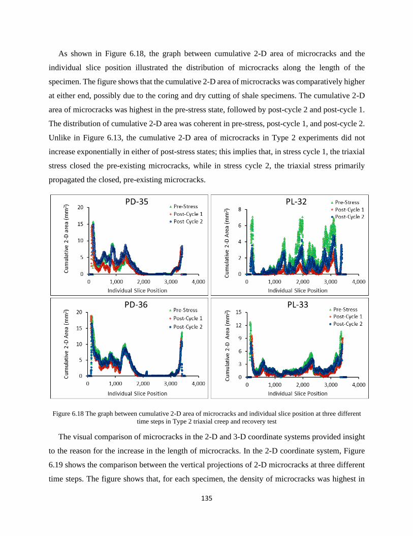
135
As shown in Figure 6.18, the graph between cumulative 2-D area of microcracks and the
individual slice position illustrated the distribution of microcracks along the length of the
specimen. The figure shows that the cumulative 2-D area of microcracks was comparatively higher
at either end, possibly due to the coring and dry cutting of shale specimens. The cumulative 2-D
area of microcracks was highest in the pre-stress state, followed by post-cycle 2 and post-cycle 1.
The distribution of cumulative 2-D area was coherent in pre-stress, post-cycle 1, and post-cycle 2.
Unlike in Figure 6.13, the cumulative 2-D area of microcracks in Type 2 experiments did not
increase exponentially in either of post-stress states; this implies that, in stress cycle 1, the triaxial
stress closed the pre-existing microcracks, while in stress cycle 2, the triaxial stress primarily
propagated the closed, pre-existing microcracks.
Figure 6.18 The graph between cumulative 2-D area of microcracks and individual slice position at three different
time steps in Type 2 triaxial creep and recovery test
The visual comparison of microcracks in the 2-D and 3-D coordinate systems provided insight
to the reason for the increase in the length of microcracks. In the 2-D coordinate system, Figure
6.19 shows the comparison between the vertical projections of 2-D microcracks at three different
time steps. The figure shows that, for each specimen, the density of microcracks was highest in

136
the pre-stress state, followed by post-cycle 2 and post-cycle 1. Some small new plane of
microcracks (enclosed in red boundary) appeared in the post-cycle 1 state compared to the pre-
stress state for specimens PD-35, PD-36, and PL-33; this shows that, although the far field triaxial
stress primarily closed the pre-existing microcracks, the high local stress also generated some new
microcracks in the specimens. Fewer small new planes of microcracks appeared in post-cycle 2
for the specimens PD-36 and PL-33 compared to the post-cycle 1. The comparison of the 3-D
projection of microcracks at three different time steps, shown in Figure 6.20, also displays similar
observations. The density of pre-existing microcracks decreased significantly in post-cycle 1.
However, the density of microcracks increased in the post-cycle 2 as compared to post-cycle 1,
such that no new major plane of microcracks formed. This implies that the increase in the area or
volume of microcracks was primarily due to the propagation of pre-existing microcracks.
As such, the comparison of microcrack geometry in Type 2 experiments showed that only the
stress history influenced the changes in the geometry of microcracks. Stress cycle 1 consolidated
both types of specimens and decreased the density of pre-existing microcracks. However, in stress
cycle 2, previously closed microcracks propagated and increased the overall density of
microcracks. The mode of decrease and increase in the area and volume of microcracks was also
independent of orientation of bedding plane; this implies that lower level of differential stress
induced a similar nature of microscopic changes in the rock specimens.

137
Figure 6.19 Comparison of vertical projection of 2-D microcracks at three different time steps in Type 2 triaxial
creep and recovery test

138

139
Figure 6.20 Three-dimensional distribution of microcracks in pre-stress, post-cycle 1, and post-cycle 2 of Type 2
triaxial creep and recovery test
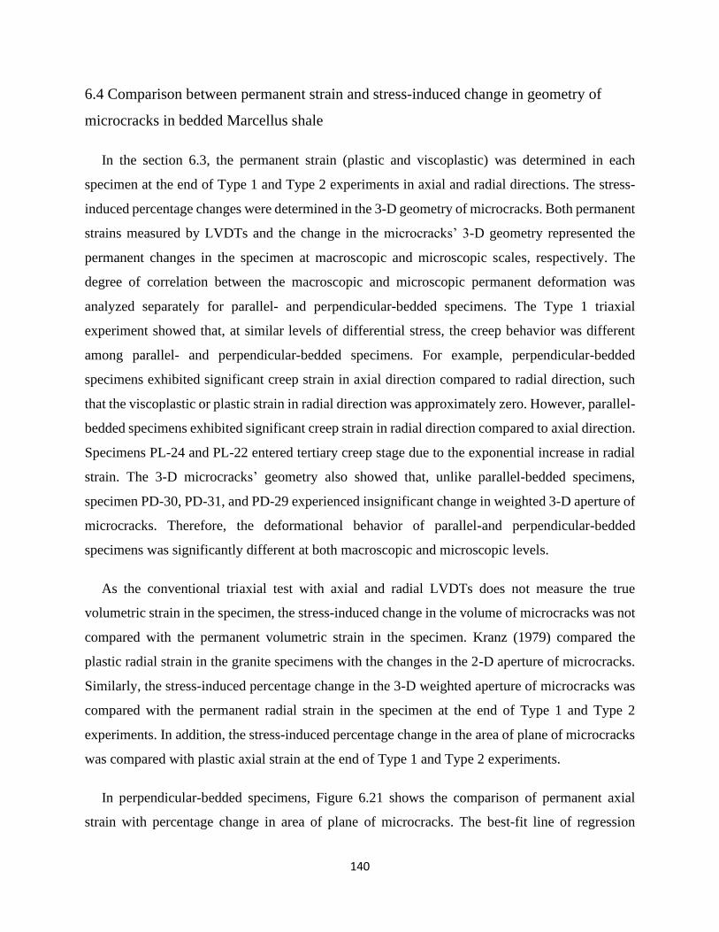
140
6.4 Comparison between permanent strain and stress-induced change in geometry of
microcracks in bedded Marcellus shale
In the section 6.3, the permanent strain (plastic and viscoplastic) was determined in each
specimen at the end of Type 1 and Type 2 experiments in axial and radial directions. The stress-
induced percentage changes were determined in the 3-D geometry of microcracks. Both permanent
strains measured by LVDTs and the change in the microcracks’ 3-D geometry represented the
permanent changes in the specimen at macroscopic and microscopic scales, respectively. The
degree of correlation between the macroscopic and microscopic permanent deformation was
analyzed separately for parallel- and perpendicular-bedded specimens. The Type 1 triaxial
experiment showed that, at similar levels of differential stress, the creep behavior was different
among parallel- and perpendicular-bedded specimens. For example, perpendicular-bedded
specimens exhibited significant creep strain in axial direction compared to radial direction, such
that the viscoplastic or plastic strain in radial direction was approximately zero. However, parallel-
bedded specimens exhibited significant creep strain in radial direction compared to axial direction.
Specimens PL-24 and PL-22 entered tertiary creep stage due to the exponential increase in radial
strain. The 3-D microcracks’ geometry also showed that, unlike parallel-bedded specimens,
specimen PD-30, PD-31, and PD-29 experienced insignificant change in weighted 3-D aperture of
microcracks. Therefore, the deformational behavior of parallel-and perpendicular-bedded
specimens was significantly different at both macroscopic and microscopic levels.
As the conventional triaxial test with axial and radial LVDTs does not measure the true
volumetric strain in the specimen, the stress-induced change in the volume of microcracks was not
compared with the permanent volumetric strain in the specimen. Kranz (1979) compared the
plastic radial strain in the granite specimens with the changes in the 2-D aperture of microcracks.
Similarly, the stress-induced percentage change in the 3-D weighted aperture of microcracks was
compared with the permanent radial strain in the specimen at the end of Type 1 and Type 2
experiments. In addition, the stress-induced percentage change in the area of plane of microcracks
was compared with plastic axial strain at the end of Type 1 and Type 2 experiments.
In perpendicular-bedded specimens, Figure 6.21 shows the comparison of permanent axial
strain with percentage change in area of plane of microcracks. The best-fit line of regression
141
between changes in the area of plane of microcracks and permanent axial strain shows that the
coefficient of determination (R2) was 0.85. No comparative analysis was performed as both
permanent radial strain and percentage changes in weighted 3-D aperture were insignificant in
perpendicular-bedded specimens. In parallel-bedded specimens, the value of R2 was 0.64 between
permanent axial strain and percentage change in the area of plane of microcracks, shown in Figure
6.22(a). Figure 6.22(b) shows that, in parallel-bedded specimens, the value of R2 was 0.55 between
permanent radial strain and percentage change in weighted 3-D aperture of microcracks. One of
the possible reasons for the small value of R2 was the significant difference in the level of accuracy
between LVDTs and magnification of the X-ray CT scanner. In addition, the radial LVDT was
always mounted onto the middle region of the cylindrical core that may have not captured the
radial dilation in the rest of the specimen. The significant value of R2 proved that the increase in
the area of plane and 3-D aperture of microcracks caused the permanent strain in axial and radial
directions, respectively.
Figure 6.21 The graph between permanent axial strain and change in area of plane of microcracks in perpendicular-
bedded specimens

142
(a)
(b)
Figure 6.22 The graph between: (a) Permanent axial strain and change in area of plane of microcracks; (b)
Permanent radial strain and change in 3-D weighted mean aperture of parallel-bedded specimens

143
6.5 Summary
The two types of triaxial creep and recovery tests showed that the bedded-shale specimens did
not experience the primary stage of creep deformation. Once the axial stress became constant, the
creep strain remained steady with time until it instantaneously entered the tertiary creep stage. The
results also showed that the creep strain was the combination of viscoelastic and viscoplastic strain.
The X-ray CT scan of the shale specimen before Type 1 and Type 2 experiments shows that each
specimen contained a significant volume of pre-existing microcracks. The comparison between
total plastic strain and stress-induced change in the geometry of the microcracks showed that the
macroscopic permanent deformation was the consequence of microscopic changes in the rock. In
addition to the level of differential stress and the duration of the constant stress state, the orientation
of the bedding planes, the volume of pre-existing microcracks, and the stress history also
influenced the creep deformation. For example, parallel-bedded specimens entered the tertiary
stage of creep deformation under the influence of radial dilation of the specimen. However, the
perpendicular-bedded specimens experienced high axial compression. The stress history in Type
2 experiments weakened the shale specimens, decreased the modulus of stiffness, and increased
the Poisson’s ratio. In Type 1 experiments, the volume of pre-existing microcracks influenced the
post-stress volume of microcracks.

144
Chapter 7 Discussions and Conclusions
In constant strain-rate experiments, small-scale microcracking is the primary reason for the
dilatancy in brittle rocks under compression (Brace et al., 1966). Scholz (1968a) analyzed the
elastic waves radiated by microcracks, compared the detected microcracks with the observed
macroscopic strains, and confirmed that the dilatancy was entirely due to the microcracking in
brittle rocks. Similarly, in uniaxial creep experiments, brittle rocks fail under dilation
(Matsushima, 1960a; Robertson, 1960), such that the creep strain in uniaxial compression, bending
and tension is directly proportional to the microcracking (Mogi, 1962; Watanabe, 1963; Brown,
1965). In the past, studies used several techniques to compare microcracking with creep strain.
Kranz (1979) visualized the microscopic growth of microcracks in Barre granite using a SEM.
Assuming the homogenous nature of granite specimens, Kranz observed that, at the end of uniaxial
creep test, the length of microcracks increased with time. Ohnaka (1983), Baud and Meredith
(1997), and Heap (2009) used acoustic emission techniques to investigate the creep mechanism in
Shinkomatsu andesite, Mannari granite, Darley Dale sandstone, Etna basalt, Bentheim sandstone,
and Crab Orchard sandstone. The comparison of the creep strain versus time curve with the
acoustic emission activity showed that the different stages of creep deformation correlated directly
with the microcracking activity in brittle rock. Okubu et al. (2008) designed a transparent triaxial
cell of acrylic resin and captured photographs of triaxially stressed brittle rock at the rate of one
image per second until the specimen failed through creep deformation. The experimental design
enabled the observation of surface cracks during creep test. Although the different experimental
methodologies involved the direct or indirect observation of microcracks during or after creep
tests, none of the techniques provided information on microcracks before the creep test. Each
technique presumed that the rock specimens were homogenous and that other factors, such as time
and level of differential stress influence the growth of the microcracks during creep the test.
In this study, the triaxial creep experiments on bedded Marcellus shale showed that the strength
of brittle shale is time-dependent. A constant stress, smaller than the time-independent strength,
led to the tertiary failure of the specimen after some interval of time. However, the creep failure
was erratic in nature. A few specimens failed before the differential stress became constant. The
time to reach faiure did not show a strong correlation with the level of differential stress. The
results of the triaxial creep experiments did not follow the empirical Norton’s creep law; that is

145
the logarithm of the rate of the secondary creep strain rate did not exhibit a linear relationship with
the logarithm of differential stress. Unlike brittle granite or quartz, which have volumes that always
increase during creep (Scholz, 1968b), shale specimens entered the tertiary creep stage of unstable
deformation either under the influence of axial compression or radial dilation. The microscopic
visualization of unstressed shale specimens using X-ray CT technique showed that each specimen
contained a significant density of pre-existing microcracks that may have developed in-situ or
during coring and dry cutting. The geometry of the microcracks, such as 2-D length, 2-D area, 2-
D aperture, 3-D volume, etc. was significantly different between the specimens. Therefore, in this
study, the application of X-ray CT technique proved that the specimens drilled from the same
block or location can be significantly different.
In this study, the application of X-ray CT technqiue proved that the intrinsic properties of the
shale, such as the orientation of bedding planes and the volume of pre-existing microcracks,
influenced the creep deformation. In the Type 1 creep and recovery experiment, parallel- and
pependicular-bedded specimens were stressed at similar levels of constant differential stress (70%
of the failure strength). Although the constant stress increased the volume of microcracks in both
orientations, the specific orientation of the bedding planes influenced the mode of increase in
volume of microcracks. Parallel-bedded specimens experienced a significant increase in the
aperture of microcracks, while perpendicular-bedded specimens only exhibited an increase in the
length of microcracks. Similarly, it was found that the presence of pre-existing microcracks
influenced the volume of microcracks after creep and recovery tests. For example, although
specimen PD-29 remained under constant stress for the longest duration of 746.77 hours, specimen
PD-30 contained the highest volume of microcracks in the post-stress state; in turn, specimen PD-
37 remained under constant stress for 360 hours and experienced macroscopic elastic behavior and
microscopic contraction of pre-existing microcracks. The volumes of pre-existing microcracks for
specimens PD-30, PD-37, and PD-29 were 771.5, 246.65, and 472.17 mm3, respectively. The
comparisons in Figure 6.8 and Figure 6.12 of Type 1 experiments show that, although the
differential stress was similar among both types of bedded specimens, the time of the applied
constant stress state did not influence the creep strain or the stress-induced changes in the area or
volume of microcracks. The comparisons in Figure 6.11 and Figure 6.17 of Type 2 experiments
show that, although the time for constant stress was constant, the differential stress did not
influence the creep strain and stress-induced change in area or volume of microcracks. Therefore,

146
it was concluded that the specimen heterogeneity and anisotropy influenced the creep behavior of
brittle shale.
The Type 1 and Type 2 triaxial creep and recovery experiments proved that constant stress
produced both viscoelastic and viscoplastic strains in the shale specimen. Although shale is a brittle
rock, the applied small stress over a long period of time did not induce strain faster than it
dissipated. Therefore, brittle shale experienced plastic flow (Nevin, 1957). As the constant
differential stress was between the yield stress and dilation stress, the instantaneously applied
stress caused both elastic and plastic strain in the shale specimens (Roylance, 2001). Therefore, at
the end of Type 1 and Type 2 creep and recovery experiments, the cumulative permanent strain
was the sum of the plastic and the viscoplastic strain. The X-ray CT equipment scanned shale
specimens either at the beginning or at the end of the Type 1 and Type 2 experimentation.
Therefore, the classification of change in the geometry of microcracks due to plastic and
viscoplastic strain was impossible. Since the microcracking caused the plastic strain in brittle rock
under compression (Scholz, 1968a) and the arithmetic sum of plastic and viscoplastic strain
exhibited positive correlation with the growth of microcracks (Figure 6.21 and Figure 6.22), it was
concluded that the microcracking caused the viscoplastic creep deformation in shale. Zaretskii and
Vyalov (1971) experimentally proved that the creep deformation of clay soils depended on stress,
time, and density of defects. Similarly, Mallet et al. (2015) proposed that the secondary creep in
brittle glass depended on temperature, stress, fluid nature, and the initial crack network or crack
density.

147
Chapter 8 Future Work
In the current research, the triaxial creep experiments on brittle Marcellus shale with
microscopic visualization using X-ray CT scan proved that the fundamental reason for the
viscoplastic creep deformation is the growth of microcracks. However, the reason for the growth
of microcracks at a constant stress state is still under investigation. One of the many theories for
the growth of microcracks in brittle rocks, e.g. quartz, granite, at a constant stress state is stress
corrosion. The phenomenon of strength reduction due to the corrosive agents at the tip of a
microcrack is called stress corrosion (Atkinson, 1984). In silicate rocks, experiments showed that
the strained Si-O-Si bonds at the crack tip, see Figure 8.1 (A), react easily with the environmental
agents like water and break, as shown in Figure 8.1 (B) (Atkinson, 1979; Michalske and Freiman,
1982). As water and aqueous solutions are abundant in the shallow crustal condition (upper 20
km), the most common mechanism of sub-critical crack growth in brittle rocks is stress corrosion
(Atkinson and Meredith, 1987; Costin, 1987). The experimental research by Sano and Kudo (1992)
and Nara et al. (2009) showed that the velocity of microcrack-tip growth in water saturated silicate
rocks was much higher than that in air. The relative humidity of air also increased the velocity of
microcracks (Nara et al., 2012). Therefore, stress corrosion, caused by moisture content, increases
the growth of sub-critical cracks and reduces the failure time of rocks.
Figure 8.1 Microcrack propagation in silica under the influence of water (A) atomistic view of a crack tip in silica
glass; (B) adsorption of water molecule at stressed Si-O-Si linkage (Rodrigues et al., 2017)
148
Although stress corrosion is a primary reason for sub-critical crack growth in monomineralic
silicate rocks, the applicability of stress-corrosion weakening reactions in complex-polymineralic
rocks is unclear (Atkinson, 1984). As the Marcellus shale is a polymineralic rock with a high
percentage of calcite, and small amount of quartz, illite and pyrite, additional laboratory
experiments would be necessary to prove the phenomenon of stress-corrosion. For example, the
moisture content test (ASTM, 2019b) and stress corrosion index for shale (Ko, 2008) could provide
useful insights about the affinity of Marcellus shale towards stress-corrosion.

149
References
Adams, L. H., & Williamson, E. D. (1923). On the Compressibility of Minerals and Rocks at
High Pressures. Journal of the Franklin Institute, 195(4), 475-529.
Ahola, M. P., Donato, D. A., & Kripakov, N. P. (1991). Application of numerical modelling
techniques to analysis of cutter roof failure. Washington D.C.: United States Bureau of
Mines.
Almasoodi, M. M., Abousleiman, Y. N., & Hoang, S. K. (2014). Viscoelastic Creep of Eagle
Ford Shale: Investigating Fluid-Shale Interaction. SPE/CSUR Unconventional Resources
Confernce (p. 8). Calgary, Canada: Society of Petroleum Engineers.
Anderson, P. M., Hirth, J. P., & Lothe, J. (2017). Theory of Dislocations 3rd edition. Cambridge
University Press, New York.
Arena, A., Piane, C. D., & Sarout, J. (2014). A new computational approach to cracks
quantification from 2D image analysis: Application to micro-cracks description in rocks.
Computers and Geosciences, 66, 106-120.
Arganda-Carreras, I., Kaynig, V., Rueden, C., Eliceiri, K. W., Schindelin, J., Cardona, A., &
Seung, H. S. (2017). Trainable Weka Segmentation: a machine learning tool for
microscopy pixel classification. Bioinformatics, 33(15), 2424-2426.
Aristorenas, G. V. (1992, May 15). Time-Dependent Behavior of Tunnels Excavated in Shale.
PhD Dissertation, Department of Civil Engineering, MIT.
Armand, G., Bumbieler, F., Conil, N., de la, V. R., Bosgiraud, J. M., & Vu, M. N. (2017). Main
outcomes from in situ thermo-hydro-mechanical experiments programme to demonstrate
feasibility of radioactive high-level waste disposal in the Callovo-Oxfordian claystone.
Journal of Rock Mechanics and Geotechnical Engineering, 9(3), 415-427.
ASTM. (2014). Standard Test Methods for Compressive Strength and Elastic Modulii of Intact
Rock Core Specimens under Varying State of Stress and Temperatures. West
Conshohocken, PA: ASTM International.
ASTM. (2016). Standard Test Methods for Creep of Rock Core Under Constant Stress and
Temperature. West Conshohocken, PA, USA: ASTM International.
ASTM. (2019). Standard Practices for Preparing Rock Core as Cylindrical Test Specimens and
Verifying Conformance to Dimensional and Shape Tolerances. West Conshohocken, PA:
ASTM International.
ASTM. (2019). Standard Test Methods for Laboratory Determination of Water (Moisture)
Content of Soil and Rock by Mass. West Conshohocken: ASTM International.
Atkinson, B. K. (1979). A fracture mechanics study of subcritical tensile cracking of quartz in
wet environments. Pure and Applied Geophysics, 117, 1011-1024.

150
Atkinson, B. K. (1984). Subcritical crack growth in Geologic Materials. Journal of Geophysical
Research, 89(B6), 4077-4114.
Atkinson, B. K., & Meredith, P. G. (1987). The theory of subcritical crack growth with
applications to minerals and rocks. In B. K. Atkinson (Ed.), Fracture Mechanics of Rock
(pp. 111-166). London: Academic Press.
Bajpayee, T. S., Pappas, D. M., & Ellenberger, J. L. (2014). Roof Instability: What Reportable
Noninjury Roof Falls in underground Coal Mines Can Tell Us. Professional Safety,
59(3), 57-62.
Barla, G., Bonini, M., & Debernardi, D. (2010). Time-dependent deformations in squeezing
tunnels. Int. J. Geoeng. Case Hist., 2(1), 819-824.
Baud, P., & Meredith, P. G. (1997). Damage accumulation during triaxial creep of Darley Dale
sandstone from pore volumometry and acoustic emission. Int. J. Rock Mech. & Min. Sci.,
34(3-4), 10.
Bauer, E. R., & Dolinar, D. R. (2000). Skin failure of roof and rib and support techniques in
underground coal mines. New Technology for Coal Mine Roof Support, pp. 99-109.
Retrieved from file:///C:/Users/Neel/Downloads/cdc_8305_DS1.pdf
Benmokrane, B., Chekired, M., & Xu, H. (1995). Monitoring Behavior of Grouted Anchors
Using Vibrating-Wire Guages. Journal of Geotechnical Engineering, 121(6), 466-475.
Berg, O. Y. (1950). On the problem of strength and plasticity of concrete. Dokladi Akademii
Bauk USSR, 70(4), 617.
Bernasconi, A. (2005). Structural analysis applied to epilepsy. In R. I. Kuzniecky, & G. D.
Jackson (Eds.), Magnetic Resonance in Epilepsy: Neuroimaging Techniques (2nd ed., p.
464). New York, NY: Elsevier.
Bernier, F., Lemy, F., Canniere, P. D., & Detilleux, V. (2017). Implications of safety
requirements for the treatment of the THMC processes in geological disposal systems for
radioactive waste. Journal of Rock Mechanics and Geotechnical Engineering, 9, 428-
434.
BGR. (2009). 50 Years BGR - An Activity Report. Hanover: Bundesanstalt für
Geowissenschaften und Rohstoffe, BGR.
Blakey, F. A., & Beresford, F. D. (1955). Tensile strains in concrete Part 1. Melbourne: CSIRO
Division of Building Research.
Boas, F. E., & Fleischmann, D. (2012). Computed tomography artifacts: Causes and reduction
techniques. Imaging in Medicine, 4(2), 229-240.
Bonini, M., Debernardi, D., Barla, M., & Barla , G. (2009). The mechanical behavior of clay
shales and implications on the design of tunnels. Rock Mechanics Rock Engineering,
42(2), 361-388.

151
Bossart, P., Jaeggi, D., & Nussbaum, C. (2017). Experiments on thermo-hydro-mechanical
behaviour of opalinus clay at Mont Terri rock laboratory, Switzerland. Journal of Rock
Mechanics and Geotechnical Engineering, 9(3), 502-510.
Boudier, T. (2014, April 16). 3D processing and analysis with ImageJ. Paris, Université Pierre et
Marie Curie, France. Retrieved from
https://imagejdocu.tudor.lu/_media/tutorial/working/workshop3d.pdf
Brace, W. F. (1978). Volume changes during frature and frictional sliding: a review. Pure Appl
Geophys, 116, 603-614.
Brace, W. F., Paulding Jr., B. W., & Scholz, C. (1966). Dilatancy in the Fracture of Crystalline
Rocks. Journal of Geophysical Research, 71(16), 3939-3953.
Brace, W. F., Silver, E., Hadley, K., & Goetze, C. (1972). Cracks and pores: A closer look.
Science, 178, 162-164.
Brantut, N., Heap, M. J., Meredith, P. G., & Baud, P. (2013). Time-dependent cracking and
brittle creep in crustal rocks: A review. Journal of Structural Geology, 52, 17-43.
Brodsky, N. S., & Munson, D. E. (1991). The effect of brine on the creep of WIPP salt in
laboratory tests. Proceedings of the 32nd U.S. Symposium on Rock Mechanics, (pp. 703-
712). University of Oklahoma, Norman.
Brown, J. W. (1965). An investigation of microseismic activity in rocj under tension. M.S.
Thesis, Pennsylvania State University.
Brown, K. E., & Jessen, F. W. (1959). Effect of pressure and temperature on cavities in salt.
Journal of Petroleum Technology, 341-345.
Buerger, M. J. (1930). Translating-Gliding in Crystals of The NaCL Structural Type. Journal
Mineralogical Society of America, 15, 174-187.
Challamel, N., Lanos, C., & Casandjian, C. (2005). Creep damage modelling for quasi-bittle
materials. Eur J. Mech., 24(4), 593-613.
Chen, R. (2009, May). Time Dependent Analysis of Tunnel in Creeping Rock. PhD Dissertation,
School of Civil Engineering, The University of Sydney, p. 257.
Chernyaev, E. (1995). Marching cubes 33: Construction of topologically correct isosurfaces.
CERN. Retrieved from
https://pdfs.semanticscholar.org/7d4b/30bbdeb1d55614e89588b7d9641c9b5a7a78.pdf
Chong, K. P., Smith, J. W., & Khaliki, B. A. (1978). Creep and Relaxation of Oil Shale. 19th
U.S. Symposium on Rock Mechanics (pp. 414-421). Reno, Nevada: American Rock
Mechanics Association.
Chow, C. K., & Kaneko, T. (1972). Automatic boundary detection of the left ventricle from
cineangiograms. Comput Biomed Res., 5, 388-410.

152
Chu, M. S., & Chang, N. Y. (1980). Uniaxial creep of oil shale under elevated temperatures. 21st
US Symposium on Rock Mechanics (pp. 207-216). Rolla, Missouri: American Rock
Mechanics Association.
Cogan, J. (1976). Triaxial creep tests of Ophonga Limestone and Ophir Shale. Int. J. Rock Mech.
Min. Sci. & Geomech. Abstr., 13, 1-10.
Compton, C., Gallagher, S., Molinda, G. M., Mark, C., & Wilson, G. (2007). Roof Screening
from Underground Coal Mines: Recent Developments. 26th International Conference on
Ground Control in Mining, (pp. 270-276). Morgantown, West Virginia .
Costin, L. S. (1987). Time-dependent deformation and failure. In B. K. Atkinson (Ed.), Fracture
Mechanics of Rock (pp. 167-216). London: Academic Press.
Crandall, D., Moore, J., Brown, S., Martin, K., Mackey, P., Paronish , T., . . . Bowers, C. (2018).
Computed Tomography Scanning and Geophysical Measurements of Core from the
Coldstream 1 MH Well. Morgantown, WV: U.S. Department of Energy, National Energy
Technology Laboratory.
Cristescu, N. (2012). Rock Rheology. Berlin: Springer.
Cristescu, N. D., & Hunsche, U. (1998). Time Effects in Rock Mechanics. John Wiley & Sons
Ltd.
Cruden, D. M. (1974). The static fatigue of brittle rock under uniaxial compression. Int. J. Rock
Mech. Min. Sci., 11, 67-73.
Das, D. (2018). Shale characterization and size-effect study using scanning electron microscopy
and x-ray diffraction. Masters Thesis, West Virginia University, p. 85.
Deng, H., Fitts, J. P., & Peters, C. A. (2016). Quantifying fracture geometry with X-ray
tomography: Technique of Iterative Local Thresholding (TILT) for 3-D image
segmentation. Computational Geosciences, 20, 231-244.
Devincre, B., Hoc, T., & Kubin, L. (2008, June). Dislocation Mean Free Paths and Strain
Hardening of Crystals. Science, 320(5884), 145-1748.
Ding, W., Li, C., Xu, C., Jiu, C., Zeng , W., & Wu, L. (2011). Fracture Development in shale and
its relationship to gas accumulation. Geoscience Frontiers, 31(1), 97-105.
Dontsova, E. (2013, January). Understanding of edge and screw dislocations in nanostructures by
modeling and simulations. Ph.D. Dissertation, The University of Minnesota, p. 129.
Doube, M., Klosowski, M. M., Arganda-Carreras, I., Cordelieres, F., Dougherty, R. P., Jackson,
J., . . . Shefelbine, S. J. (2010). BoneJ: free and extensible bone image analysis in ImageJ.
Bone, 47(6), 1076-1079.
Dougherty, R., & Kunzelmann, K. (2007). Computing Local Thickness of 3D Structures with
ImageJ. Microscopy and Microanalysis, 13(S02), 1678-1679.

153
Dusseault, M. B., & Fordham, C. J. (1993). Time-dependent behavior of rocks. In J. A. Hudson
(Ed.), Comprehensive Rock Engineering (Vol. 3, pp. 119-149). Pergamon Press.
Evans, R. H. (1936). The elasticity and plasticity of rocks and artifical stones. Proceedings of the
Leeds Philosophical and Literary Society (scientific section), 3(3), 145-158.
Fakhimi, A., & Fairhurst, C. (1994). A model for the time-dependent behavior of rock. Int. J.
Rock Mech. Min. Sci. Geomech. Abstr., 31, 117-126.
Ferreira, T., & Rasband, W. S. (2012). ImageJ User Guide. Retrieved from
https://imagej.nih.gov/ij/docs/guide/
Flohr, M. J. (1997, May). X-ray Powder Diffraction. Retrieved from USGS Information
Handout: https://pubs.usgs.gov/info/diffraction/html/
Friedel, J. (1967). Dislocations. Pergamon, Oxford.
Gadde, M. M., & Peng, S. S. (2005a). Effect of in-situ stresses on the stability of coal mine
development workings. 21st International Conference on Ground Control in Mining, (pp.
162-168). Morgantown.
Gadde, M. M., & Peng, S. S. (2005b). Numerical simulation of cutter roof failure under weak
roof conditions. Society for Mining, Metallurgy and Exploration. Salt Lake City, Utah.
Gao, F., & Stead, D. (2013). Discrete element modelling of cutter roof failure in coal mine
roadways. International Journal of Coal Geology, 116, 158-171.
Ghosh Roy, M., & Rao, K. S. (2015). Analysis of creep behaviour of soft rocks in tunneling.
ISEG-EGNM, (p. 12).
Gnos, E., & et al. (2010). Sayh al Uhaymir: A new martian meteorite from the Oman desert.
Meteorites and Planetary Sciences, 37(6), 835-854.
Gold, L. W. (1960). The Cracking Activity in Ice During Creep. Canadian Journal of Physics,
38(9), 1137-1148.
Griggs, D. (1939). Creep of Rocks. The Journal of Geology, 47(3), 225-251.
Griggs, D. W. (1940). Experimental flow of rocks under conditions favoring recrystallization.
Geol. Soc. Amer. Bull., 51, 1001-1022.
Guo, D., Qu, X., Du, X., Wu, K., & Chen, X. (2014). Salt and Pepper Noise Removal with Noise
Detection and a Patch-Based Spare Representation. Advances in Multimedia, 14.
Guo, J., & Liu, Y. (2012). Modeling of Proppant Embedment: Elastic Deformation and Creep
Deformation. SPE International Production and Operations Conference and Exhibition
(p. 8). Doha, Qatar: Society of Petroleum Engineers.
Haasen, P. (1974). Physical Metallurgy. Berlin: Springer-Verlag.

154
Haimson, B. C. (1978). Effect of Cyclic Loading on Rock. Dynamic Geotechnical Testing, 228-
245.
Hansen, F. D., Hardin, E. L., & Rechard, R. P. (2010). Shale Disposal of U.S. High-Level
Radioactive Waste. Albuquerque, New Mexico: Sandia National Laboratories.
He, M. (1998, June). Application of X-ray tomography to measurement of fractures in rocks.
Masters Thesis, Stanford University, p. 91.
Heap, M. J. (2009). Creep: Time-dependent brittle deformation in rocks. PhD Dissertation,
University College London.
Heard, H. C. (1960). Chapter 7: Transition from brittle fracture to ductile flow in Solenhofen
limestone as a function of temperature, confining pressure, and interstitial fluid pressure.
Rock Deformation. 79, pp. 193-226. Geological Society of America.
doi:10.1130/MEM79-p193
Hess, H. H., Adkins, J. N., Benson, W. E., Frye, J. C., Heroy, W. B., Hubert, M. K., . . . Theis, C.
V. (1957). Disposal of Radioactive waste on land. Waste Disposal of the Division of
Earth Sciences, National Academy of Sciences-National Research Council, Washington.
Hill, J. L. (1986). Cutter roof failure: an overview of the causes and methods for control.
Washington D.C.: United States Bureau of Mines.
Hobbs, D. W. (1970). Stress-Strain-Time Behavior of a Number of Coal Measure Rocks.
International Journal of Rock Mechanics and Mining Sciences, 7, 149-170.
Hoek, E., & Bown, E. T. (1980). Underground Excavations in Rock. Boca Raton, FL: CRC
Press.
Horii, H., & Nemat-Naseer, S. (1985). Compression-Induced Microcrack Growth in Brittle
Solids: Axial Splitting and Shear Failure. Journal of Geophysical Research, 90(B4),
3105-3131.
Hsu, T., Slate, F., Sturman, G., & Winter, G. (1963). Microcracking of Plain Concrete and the
Shape of the Stress-Strain Curve. ACI Journal, 60(14), 209-224.
Hu, B., Yang, S. Q., Xu, P., & Cheng , J. L. (2019). Cyclic loading-unloading creep behavior of
composite layered specimens. Acta Geophysica, 67, 449-464.
Hull, D. (2011). Introduction to dislocations 5th Edition. (D. J. Bacon, Ed.) Oxford:
Butterworth-Heinemann.
Illston, J. M. (1978). Creep of Concrete. In C. D. Pomeroy (Ed.), Creep of Engineering Materials
(pp. 47-66). Cambridge, Great Britain: Heffers Printers Ltd.
Jaeger, J. C., Cook, N. G., & Zimmerman, R. (1976). Fundamentals of Rock Mechanics. London:
Chapman and Hall.
155
Jia, L., Chen, M., & Jin, Y. (2014). 3D imaging of fracture in carbonate rocks using X-ray
computed tomography technology. Carbon Evaporites, 29(2), 147-153.
Jones, R. (1952). A method of studying the formation of cracks in a material ssubjected to stress.
British Journal of Applied Physics, 3, 229-232.
Karacan, C. O. (2003). Heterogenous sorption and swelling in a confined and stressed coal
during CO2 injection. Energy & Fuels, 17, 1595-1608.
Kendall, M. A. (1958). An investigation of the creep phenomena exhibited by Solenhofen
limestone, halite, and cement under medium confining pressure. Master's Thesis,
Agricultural and Mechanical College of Texas, p. 54.
Khosravi, E. (2017). An Experimental Investigaton on Creep Behavior of Shale Rocks: With
Emphasis on the Influence of Temperature and Anisotropy. Masters Dissertation,
University of Oklahoma.
Kim, Y. R., Guddati, M. N., Underwood , B. S., Yun, T. Y., Subramanian, V., & Savadatti, S.
(2009). Development of a Multiaxial Viscoelastoplastic Continuum Damage Model for
Asphalt Mixtures. U.S. Department of Transportation.
King, G. C., Stein, R. S., & Lin, J. (1994). Static Stress Changes and the Triggering of
Earthquakes. Bulletin of the Seismological Society of America, 84(3), 935-953.
Klemetti, T., Oyler, D., & Molinda, G. M. (2009). Time Dependent Roof Deterioration at a
Central Ohio Coal Mine. 28th International Conference on Ground Control in Mining,
(pp. 248-255). Morgantown, West Virginia.
Ko, T. Y. (2008). Subcritical crack growth under Mode I, II, and III loading for Coconico
Sandstone. Ph.D. Dissertation, The University of Arizona.
Kranz, R. L. (1979). Crack Growth and Development During Creep of Barre Granite. Int. J. Rock
Mech. Min. Sci. & Geomech. Abstr., 16, 23-35.
Kranz, R. L. (1980). The Effect of Confining Pressure and Stress Difference on Static Fatigue of
Granite. Journal of Geophysical Research, 85, 1854-1866.
Kranz, R. L., & Scholz, C. H. (1977). Critical Dilatant Volume of Rocks at the Onset of Tertiary
Creep. Journal of Geophysical Research, 82(No. 30), 4893-4898.
Kranz, R. L., Harris, W. J., & Carter, N. L. (1982). Static Fatigue of granite at 200 degree C.
Geophysical Research Letters, 9, 1-4.
Krumbein, W. C., & Sloss, L. L. (1963). Stratigraphy and Sedimentation. San Francisco: W.H.
Freeman and Co. .
Lee, T.-C., Kashyap, R. L., & Chu, C.-N. (1994). Building Skeleton Models via 3-D Medial
Surface/Axis Thinning Algorithms. CVGIP: Graphical Models and Image Processing,
56(6), 462-478.
156
Lenoir, N., & et al. (2007). Volumetric digital image correlation applied to X-ray
microtomography images from triaxial compression tests on argillaceous rock. Strain,
43(3), 193-205.
Lester, J. M., Brenner, J. F., & Selles, W. D. (1980). Local transforms for biomedical image
analysis. Comp Graph Imag Proc., 13, 17-30.
Li, Y., & Ghassemi, A. (2012). Creep Behavior of Barnett, Haynesville and Marcellus Shale.
46th U.S. Rock Mechanics/Geomechanics Symposium (p. 7). Chicago, IL: American
Rock Mechanics Association.
Li, Z., Nguyen, T. S., Su, G., Labrie, D., & Barnichon, J. D. (2016). Development of a
viscoelastoplastic model for a bedded argillaceous rock from laboratory triaxial tests.
Canadian Geotechnical Journal, 54, 359-372.
Liu, J., & Zhou, R. (2000). Mechanical Effects of Water Content in the Creep Parameters. 4th
North American Rock Mechanics Symposium (p. 5). Seattle, Washington: American Rock
Mechanics Association.
Liu, S., Wang, Z., & Zhang, L. (2018). Experimental study on the cracking process of layered
shale using X-ray microCT. Energy Exploration & Exploitation, 36(2), 297-313.
Lo, K. Y., & Lee, Y. N. (1990). Time-dependent deformation behaviour of Queenston shale.
Canadian Geotechnical Journal, 27(4), 461-471.
Lo, K. Y., Wai, R. S., Palmer, J. H., & Quigley, R. M. (1978). Time-dependent deformation of
shaly rocks in Southern Ontario. Candaian Geotechnical Journal, 15(4), 537-547.
Lora, R. F. (2015). Geomechanical characterization of Marcellus Shale. Graduate College
Dissertation and Thesis, University of Vermont.
Lorensen , W. E., & Cline, H. E. (1987). Marching cubes: A high resolution 3D surface
construction algorithm. 14th Annual Conference on Computer Graphics and Interactive
Techniques, (pp. 163-169). doi:10.1145/37401.37422
Main, I. G., & Meredith, P. G. (1991). Stress corrosion constitutivr laws as a possible mechanism
of intermediate-term and short-term seismic quiescence. Geophysical Journal
International, 107(2), 363-372.
Mallet, C., Fortin, J., Gueguen, Y., & Bouyer, F. (2015). Brittle creep and subcritcial crack
propagation in glass submitted to triaxial conditions. Journal of Geophysical Research:
Solid Earth, 120, 879-893.
Mark, C., Molinda, G. M., Burke, L., & Padgett, P. (2004). Preventing Falls of Ground in Coal
Mines with Exceptionally Low-Strength Roof: Two Case Studies. 23rd International
Conference on Ground Control in Mining, (pp. 220-227). Morgantown, West Virginia.
Martin, R. J. (1972). Time-dependent crack growth in quartz and its application to the creep of
rocks. Journal of Geophysical Research, 77, 1406-1419.
157
Matsushima, S. (1960a). On the flow and fracture of igneous rocks. Disaster Prevention
Research Institute Kyoto University Bulletin, 36(2).
Matsushima, S. (1960b). Variation of the elastic wave velocities of rocks in the process of
deformation and fracture under high pressure. Disaster Prevention Research Institute
Kyoto University Bulletin, 32, pp. 1-8.
Medhurst, T., Hatherly, P., & Hoyer, D. (2014). Investigation of the relationship between strata
characteristics and longwall caving behavior. 14th Coal Operator's Conference, (pp. 51-
62). The University of Wollongong, Australia.
Mehta, P. K., & Monteiro, P. J. (2006). Concrete: Microstructure, properties, and materials.
New York: McGraw-Hill.
Michalske, T. A., & Freiman, S. W. (1982). A molecular interpretation of stress corrosion in
silica. Nature, 295, 511-512.
Mining Facts - 2015. (n.d.). Retrieved from CDC:
https://www.cdc.gov/niosh/mining/works/statistics/factsheets/miningfacts2015.html
Mishra, B., & Verma, P. (2015). Uniaxial and triaxial single and multistage creep tests on coal-
measure shale rocks. International Journal of Coal Geology, 137(1), 55-65.
Mogi, K. (1962). Study of the elastic shocks caused by the fracture of a heterogenous material
and its relation to earthquake phenomena. Bull. Earthquake Res. Inst. Tokyo Univ., 40,
125.
Mogi, K. (2006). Experimental Rock Mechanics. London: CRC Press.
Mohapatra, S. (2012, December). Development and Quantitative Assessment of a Beam
Hardening Correction Model for Preclinical Micro-CT. Masters Thesis, The University of
Iowa, p. 91.
Molinda, G. M. (2003). Geologic Hazards and Roof Stability in Coal Mines. CDC NIOSH
Information Circular 9466.
Molinda, G. M., & Klemetti, T. (2008). Diagnosing and Controlling Moisture-Sensitive Roof in
Coal Mines. Electron J Geotech Eng, 13(A), 1-20.
Molinda, G. M., & Mark , C. (2010). Ground Failures in Coal Mines with Weak Roof. Electron
Journal of Geotechnical Engineering, 15(F), 547-588.
Molinda, G. M., & Mark, C. (1996). Rating the strength of coal mine roof rocks. Pittsburgh, PA:
US Department of Interior, Bureau of Mines.
Molinda, G. M., Oyler, D. C., & Gurgenli, H. (2006). Identifying Moisture Sensitive Roof Rocks
in Coal Mines. 25th International Conference on Ground Control in Mining, (pp. 57-64).
Morgantown, West Virginia.

158
Murphy, M. M. (2016). Shale Failure Mechanics and Intervention Measures in Underground
Coal Mines: Results from 50 years of Ground Control Safety Research. Rock Mechanics
and Rock Engineering, 49(2), 661-671.
Nara, Y., Morimoto, K., Hiroyoshi, N., Yoneda, T., Kaneko, K., & Benson, P. M. (2012).
Influence of relative humidity on fracture toughness of rock: Implications for subcritical
crack growth. International Journal of Solids and Structures, 49, 2471-2481.
Nara, Y., Takada, M., Igarashi, T., Hiroyoshi, N., & Kaneko, K. (2009). Subcritical crack growth
in rocks in an aqueous environment. Explor. Geophys., 40, 163-171.
Nettleton, L. L. (1934). Fluid mechanics of salt domes. American Association of Petroleum
Geologists Bulletin, 18, 1175-1204.
Nevin, C. M. (1957). Principles of Structural Geology. (F. Edition, Ed.) New York: John Wiley
& Sons, Inc.
Nishihara, M. (1952). Creep of shale and sandy shale. J. geol. Soc. Jpn., 58, 373-377.
Nithya, K., Karthik, K., & Ramasamy, K. (2014). Comparison of Contrast Enhancement
Technique with Partitioned Iterated Function System. International Journal of Scientific
& Engineering Research, 5(5), 167-172.
Ode, H. (1968). Review of Mechanical Properties of Salt Relating to Salt-Dome Genesis. The
Geological Society of America, 88, 53-78.
Ohnaka, M. (1983). Acoustic emission during creep of brittle rock. International Journal of Rock
Mechanics and Mining Sciences & Geomechanics Abstracts, 20(3), 121-134.
Okubu, S., Fukui, K., & Hashiba, K. (2008). Development of a transparent triaxial cell and
observation of rock deformation in compression and creep tests. International Journal of
Rock Mechanics and Mining Sciences, 45(3), 351-361.
Ottner, F., Gier, S., Kuderna, M., & Schwaighofer, B. (2000). Results of an inter-laboratory
comparison of methods for quantitative clay analysis. Applied Clay Science, 17, 223-243.
Pappas, D. M. (1987). Roof and rib fall accident and cost statistics: an indepth study. Pittsburgh,
PA: U.S. Department of the Interior, Bureau of Mines.
Pappas, D. M., & Mark, C. (2012). Roof and rib fall incident trends: a 10-year profile. Trans Soc
Min Metal Explor, 330, 462-478.
Pappas, D. M., Bauer, E. R., & Mark, C. (2000). Roof and Rob Fall Incidents and Statistics: A
Recent Profile. New Technology for Coal Mine Roof Support (pp. 3-21). CDC-NIOSH,
Information Circular 9453.
Pappas, D., & Mark, C. (2010). Roof and Rib Fall Accidents and Statistics - An Update, in
Characterization and Control of Coal Mine Roof in Weak Ground. NIOSH Information
Circular .

159
Parker, F. L., Boegly, W. J., Bradshaw, R. L., Crowell, J., Eastwood, E. R., Empson, F. M., . . .
Struxness, E. G. (1959). Status Report on Waste Disposal in Natural Salt Formation. Oak
Ridge National Laboratory.
Parsons, R. C., & Hedley, D. (1966). The Analysis of the Viscous Property of Rocks For
Classification. Int. J. Rock Mech. Min. Sci., 3, 323-335.
Patterson, M. S., & Wong, T. F. (2005). Experimental Rock Deformation - The Brittle Field.
Springer.
Paulding Jr., B. W. (1965). Crack growth during brittle fracture in compression. Ph.D. Thesis,
MIT.
Pecharsky, V. K., & Zavalij, P. Y. (2009). Fundamentals of Powder Diffraction and Structural
Characterization of Materials, 2nd Edition. Verlag, US: Springer.
Pellet, E., Roosefid, M., & Deleruyelle, F. (2009). On the 3D numerical modelling of the time-
dependent development of the damage zone around underground galleries during and
after excavation. Tunnelling and Underground Space Technology, 24, 665-674.
Peng, S. S. (2015). Topical areas of research needs in ground control - A state of the art review
on coal mine ground control. International Journal of Mining Science and Technology,
25, 1-6.
Peng, S. S., & Johnson, A. M. (1972). Crack growth and faulting in cylindrical specimens of
Chelmsford granite. Int. J. Rock Mech. Min. Sci., 9, 37-86.
Phillips, D. W. (1931). Further Investigation of physical properties of coal measure rocks and
experimental work on the development of fractures. Transactions of the Institution of
Mining Engineers, 82, 432-450.
Plessis, A. D., Broeckhoven, C., Guelpa, A., & Roux, S. I. (2017). Laboratory X-ray micro-
computed tomography: a user guideline for biological samples. Gigascience, 6(6), 1-11.
Popova, O. (2017). Marcellus Shale Play: Geology review. Independent Statistics and Analysis,
U.S. Energy Information Administration.
Price, N. J. (1964). A study of the time-strain behavior of coal measure rocks. International
Journal of Rock Mechanics and Mining Sciences, 1, 277-303.
Ray, A. K. (2009). Influence of cutting sequence and time effects on cutters and roof falls in
underground coal mine- numerical approach. Ph.D. Dissertation.
Rinehart, J. S. (1965). Dynamic fracture strength of rocks. Proceedings of the seventh US Rock
Mechanics Symposium, (pp. 205-208).
Rinne, F. (1926). Ûber kübstlich und natürlich umgeformtes Steinsalz. Centrbl. Mineral., 355-
358.
Robertson, E. C. (1960). Creep in Solenhofen Limestone. Geol. Soc. Am. Mem., 79, 227.

160
Rodrigues, B. P., Huhn, C., Erlebach, A., & Mey, D. e. (2017). Parameterization in models of
subcritical glass fracture: Activation offset and concerted activation. Frontiers in
Materials, 4(20).
Rodriguez, R., Crandall, D., Song, X., Verba, C., & Soeder, D. (2014). Imaging Techniques for
Analyzing Shale Pores and Minerals. Morgantown, WV: U.S. Department of Energy,
National Energy Technology Laboratory.
Roen, J. B. (1984). Geology of the Devonian black shales of the Appalachian Basin. Organic
Geochemistry, 5(4), 241-254.
Romano, C., Minto, J., Shipton, Z. K., & Lunn, R. (2018). Automated high accuracy, rapid beam
hardening correction in X-ray Computed Tomography of multi-mineral, heterogenous
core samples. InterPore 2018. New Orleans.
Rongzun, H., Zuhui, Z., & Jingen, D. (1987). The Creep Characteristics of Shale Formation And
the Analysis of Its Loading On the Oil Well Casing. 6th ISRM Congress. Montreal,
Canada: International Society of Rock Mechanics and Rock Engineering.
Rouabhi, A., Tijani, M., & Rejeb, A. (2007). Triaxial behavior of transversely isotropic
materials: Application to sedimentary rocks. International Journal for Numerical and
Analytical Methods in Geomechanics, 31, 1517-1535.
Rowe, T., & et al. (2001). Forensic palentology: The archaeoraptor forgery. Nature, 410, 539-
540.
Roylance, D. (2001, August 23). Stress-strain curves. Retrieved from
http://web.mit.edu/course/3/3.11/www/modules/ss.pdf
Sakthivel, N., & Prabhu, L. (2014). Mean-Median filtering for implusive noise removal.
International Journal of Basics and Applied Sciences, 2(4), 47-57.
Sano, O., & Kudo, Y. (1992). Relation of fracture resistance to fabric for granitic rocks. Pure
Applied Geophysics, 138, 657-677.
Savage, W. Z., & Braddock, W. A. (1991). A Model for Hydrostatic Consolidation of Pierre
Shale. Int. J. Rock Mech. Min. Sci. & Geomech. Abstr., 28(5), 345-354.
Schindelin, J., Arganda-Carreras, I., Frise, E., Kaynig, V., Longair, M., Pietzsch, T., . . .
Cardona, A. (2012). Fiji: an open-source platform for biological-image analysis. Nature
methods, 9(7), 676-682. doi:10.1038/nmeth.2019
Schmid, P. (1999). Segmentation of digitized dermatoscopic images by two-dimensional color
clustering. IEEE Trans on Med Imag., 18(2), 164-171.
Schock, R. N., Heard, H. C., & Stephens, D. R. (1973). Stress-strain behavior of a granodiorite
and two graywackes on compression to 20 kilobars. Journal of Geophysical Research,
78, 5922-5941.

161
Scholz, C. H. (1968a). Microfracturing and the inelastic deformation of rock in compression.
Journal of Geophysical Research, 73(No. 4), 1417-1432.
Scholz, C. H. (1968b). Mechanism of creep in brittle rock. Journal of Geophysical Research, 73,
3295-3302.
Scholz, C. H. (2002). The Mechanics of Earthquake and Faulting, second edition. Cambridge
University Press, Cambridge, United Kingdom.
Scintag, I. (1999). Chapter 7: Basics of X-ray Diffraction. Retrieved from
http://www.geo.umass.edu/courses/geo311/xrdbasics.pdf
Sellars, E., Vervoort, A., & Cleyenenbreugel, J. V. (2003). Three-dimensional visualization of
fractures in rock test samples, simulating deep level mining excavations, using X-ray
computed tomography. Geological Society, London, Special Publications, 215, 69-80.
Senseny, P. E. (1983). Review of constitutive laws used to describe the creep of salt.
International Journal of Mining Engineering, 2(4), 323-340.
Senseny, P. E. (1985). Determination of a Constitutive Law for Salt at Elevated Temperatures
and Pressure. (H. J. Pincus, & E. R. Hoskins, Eds.) Measurement of Rock Properties at
Elevated Pressures and Temperatures, ASTM STP 869, 55-71.
Senseny, P. E., Hansen, F. D., Russell, J. E., Carter, N. L., & Handin, J. W. (1992). Mechanical
Behaviour of Rock Salt: Phenomenology and Micromechanisms. Int. J. Rock Mech. Min.
Sci. & Geomech. Abstr., 29(4), 363-378.
Serata, S. (1959). Reactor fuel waste disposal project-- development of design principle for
disposal of reactor fuel waste into underground salt cavities. University of Texas, Civil
Engineering, Saniatry Engineering Research Laboratory.
Shalabi, F. I. (2005). FE analysis of time-dependent behavior of tunneling in squeezing ground
using two different creep models. Tunnelling and Underground Space Technology, 20,
271-279.
Sharifzadeh, M., Tarifard, A., & Moridi, M. A. (2013). Time-dependent behavior of tunnel lining
in weak rock mass based on displacement back analysis method. Tunnelling and
Underground Space Technology, 38, 348-356.
Silva, A. L., Oliveira, A. H., & Fernandes, M. L. (2011). Influence of preferred orientation of
minerals in the mineralogical identification process by X-ray diffraction. 2011
International Nuclear Atlantic Conference, (pp. 1-11). Belo Horizonte, MG, Brazil.
Singh, D. P. (1975). A Study of Creep of Rocks. Int. J. Rock Mech. Min. Sci. & Geomech. Abstr.,
12, 271-276.
Soldal, M., Wilkinson, H. D., Viken, I., & Sauvin, G. (2017). Rock visualization using micro-CT
scanner and X-ray transparent triaxial apparatus. International Symposium of the Society
of Core Analysts, (p. 9). Vienna, Austria.

162
Sone, H. (2012). Mechanical Properties of Shale gas Reservoir Rocks and its relation to the In-
situ stress Variation Observed in Shale Gas Reservoirs. PhD Dissertation, Department of
Geophysics, Stanford University.
Sone, H., & Zoback, M. D. (2011). Visco-plastic Properties of Shale Gas Reservoir Rocks. 45th
U.S. Rock Mechanics/Geomechanics Symposium (p. 7). San Francisco, CA: American
Rock Mechanics Association.
Sone, H., & Zoback, M. D. (2014). Time-dependent deformation of shale gas reservoir rocks and
its long-term effect on the in situ state of stress. International Journal of Rock Mechanics
and Mining Sciences, 69, 120-132.
Sonka, M., Hlavac, V., & Boyle, R. (1999). Image Processing, Analysis, and Machine Vision.
Pacific Grove, CA: PWS Publishing.
Sprunt, E. S., & Brace, W. F. (1974). Direct Observation of Microcavities in Crystalline Rocks.
Int. J. Rock Mech. Min. Sci. & Geomech. Abstr., 11, 139-150.
Standard Operating Procedure: PANalytical X'Pert PRO XRD. (2014). Retrieved from WVU
Shared Research Facilities: https://sharedresearchfacilities.wvu.edu/files/d/c88d36dd-
7c59-4753-91cc-e0c23b53ab37/srf_panalytical-xrd_sop_2014.pdf
Stevenson, J. J. (1913). The Formation of Coal Beds. IV. Proceedings of the American
Philosophical Society, 52(208), 31-162.
Stocke, K., & Borchert, H. (1936). Fliessgrenzen von Salzgesteinen und Salztektonik. Kali, 20,
191-194, 204-207, 214-217.
Su, W. H., & Peng, S. S. (1987). Cutter roof and its causes. Mining Science and Technology, 4,
113-132.
Taheri, A., Hamzah, N., & Dai, Q. (2017). Degradation and improvement of mechanical
properties of rock under triaxial compressive cyclic loading. Japanese Geotechnical
Society Special Publication, 5(2), 71-78.
Tapponnier, P., & Brace, W. F. (1976). Development of stress-induced microcracks in Westerly
Granite. Int. J. Rock Mech. Min. Sci. & Geomech. Abstr., 13, 103-112.
Taylor, G. I. (1934). The Mechanism of Plastic Deformation of Crystals. Part I. Theoretical.
Proceedings of the Royal Society of London, 145(855), 362-387.
Tewalt, S. J., Ruppert, L. F., Bragg, L. J., Carlton, R. W., Brezinski, D. K., Wallack, R. N., &
Butler, D. T. (2001). A Digital Resource Model of the Upper Pennsylvanian Pittsburgh
Coal Bed, Monogahela Group, Northern Appalachian Basin Coal Region. U.S.
Geological Survey Professional Paper 1625-C.
Tocher, D. (1957). Anisotropy in rocks under simple compression. Trans. Am. Geophys. Union,
38, 89-94.

163
Varo, L., & Passaris, E. (1977). The role of water on the creep properties of halite. Conference
on Rock Engineering, University of Newcastle, (pp. 85-100). Tyne, U.K.
Watanabe, H. (1963). The occurence of elastic shocks during destruction of rocks and its relation
to the sequence of earthquakes. Geophysical papers dedicated to Professor Kenso Sassa,
653-658.
Wawersik, W. R., & Brace, W. F. (1971). Post-failure behavior of granite and diabase. Rock
Mechanics and Rock Engineering, 3, 61-85.
Wawersik, W. R., & Brown, W. S. (1973). Creep fracture in rock. Salt Lake City: Department of
Mechanical Engineering, Utah University.
Weertman, J. (1955). Theory of Steady-State Creep Based on Dislocation Climb. Journal of
Applied Physics, 26(10), 1213-1217.
Weidinger, P., Blum, W., Hunsche, U., & Hampel, A. (1996). The influence of friction on plastic
deformation in compression tests. Physica Status Solidi A, 156, 305-315.
Weidinger, P., Hampel, A., Blum, W., & Hunsche, U. (1997). Creep Behaviour of natural rock
salt and its description with the composite model. Materials Science and Engineering A,
234-236, 646-648.
Wu, F. T., & Thomsen, L. (1975). Microfracturing and Deformation of Westerly Granite Under
Creep Condition. Int. J. Rock Mech. Min. Sci. & Geomech. Abstr., 12, 167-173.
Xradia. (2010, April). MicroXCT-200 and MicroXCT-400 User's Guide. Version 7.0, Revision
1.5.
Yadav, G., Maheshwari, S., & Agarwal, A. (2014). Contrast Limited Adaptive Histogram
Equalization Based Enhancement for Real Time Video System. International Conference
on Advances in Computing, Communications and Informatics (pp. 2392-2397). Delhi,
India: IEEE.
Yang, X., Lu, J.-H., Wang, C.-P., & Deng, J. (2016). Experimental study of high-temperature
fracture propagation in anthracite and destruction of mudstone from coalfield using high-
resolution microfocus X-ray computed tomography. Rock Mechanics and Rock
Engineering, 49(9), 3723-3734.
Yu, B., Bradley, R. S., Soutis, C., & Withers, P. J. (2016). A comparison of different approaches
for imaging cracks in composites by X-ray microtomography. Philos Trans R Soc A, 374,
15.
Yu, L., Weetjens, E., Sillen, X., Vietor, T., Li, X., Delage, P., . . . Charlier, R. (2014).
Consequences of the Thermal Transient on the Evolution of the Damaged Zone Around a
Repository for Heat-Emitting High-Level Radioactive Waste in a Clay Formation: a
Performance Assessment Perspective. Rock Mechanics and Rock Engineering, 47(3), 3-
19.

164
Zaretskii, Y. K., & Vyalov, S. S. (1971). Structural Mechanics of Clay Soils. Soil Mechanics and
Foundation Engineering, 8(3), 153-160.
Zhang, C.-L. (2018). Thermo-hydro-mechanical behavior of clay rock for deep disposal of high-
level radioactive waste. Journal of Rock Mechanics and Geotechnical Engineering, 10,
992-1008.
Zhang, Q. B., & Zhao, J. (2014). A review of dynamic experimental techniques and mechanical
behaviour of rock materials. Rock Mech Rock Eng, 47, 1411-1478.
Zhang, Y., Xu, W.-y., Shao, J.-f., Zhao, H.-b., & Wang, W. (2015). Experimental investigation
of creep behavior of clastic rock in Xiangjiaba Hydropower Project. Water Science and
Engineering, 8(1), 55-62.
Zuidervald, K. (1994). Contrast limited adaptive histogram equalization. In P. S. Heckbert (Ed.),
Graphic Gems IV (pp. 474-485). Academic Press Professional, Inc. San Deigo, CA,
USA.
Zwicky, F. (1923). Physik. Z., 24, 131.

165
Appendix
A. Macro to enhance contrast and segment microcracks – Case IV

166
B Macro for calculating area, weighted-mean aperture, and length of microcracks of an
individual 2-D image in FIJI

167
C. Script to summarize the 2-D geometry of microcracks in MATLAB

168
D. Comparison between Measured and Calculated Volume of 3-D Rectangular
Microcrack
In Table D.1, the measured volume, aperture and area of x-z plane is determined through the
approach explained in section 5.3.2. In addition, the calculated volume of microcracks is the
product of the area of plane of microcracks (oriented perpendicular to the direction of aperture)
and measured aperture of microcracks. Figure D.1 shows the comparison between measured and
calculated volume of microcracks. The high value of degree of determination (i.e. R2 = 0.99) of
the best-fit, least square regression line indicates that both parameters are in perfect correlation. In
addition, the slope of 1.202 represents that both parameters are equivalent, proving that the
presumption that the 3-D microcrack can be assumed as a rectangular plate is valid.
Table D.1 Measured and Calculated 3-D geometrical parameters
Specimen ID Measured
volume (mm3)
Measured aperture
(mm)
Measured Area
of plane (mm2)
Calculated
Volume (mm3)
PD-30_Pre-Stress 771.50 0.14 5,859.09 796.84
PD-31_Pre-Stress 507.36 0.13 4,052.42 506.55
PD-37_Pre-Stress 232.86 0.13 1,708.38 220.38
PD-29_Pre-Stress 472.17 0.12 3,665.60 454.53
PL-23_Pre-Stress 936.22 0.14 7,619.83 1,051.54
PL-24_Pre-Stress 294.93 0.12 2,553.07 293.60
PL-34_Pre-Stress 123.74 0.11 1,072.38 113.67
PL-22_Pre-Stress 803.75 0.13 6,614.32 826.79
PD-30_Post Stress 1,186.90 0.14 9,046.73 1,221.31
PD-31_Post Stress 617.24 0.12 5,196.51 644.37
PD-37_Post Stress 148.24 0.09 1,119.43 105.23
PD-29_Post Stress 764.09 0.13 6,381.84 823.26
PL-23_Post Stress 1,063.29 0.16 7,487.84 1,198.05
PL-24_Post Stress 1,883.80 0.17 13,131.33 2,179.80
PL-34_Post Stress 618.19 0.15 4,201.41 609.20
PL-22_Post Stress 4,521.66 0.20 26,505.35 5,407.09
PD-35_Pre-Stress 231.71 0.13 1,635.77 206.11
PD-36_Pre-Stress 330.04 0.13 2,434.91 323.84
PL-32_Pre-Stress 185.24 0.09 1,205.07 109.66
PL-33_Pre-Stress 208.95 0.13 1,335.86 166.98

169
PD-35_Post_Cycle1 166.04 0.12 1,306.04 160.64
PD-36_ Post_Cycle1 240.46 0.12 1,968.35 240.14
PL-32_ Post_Cycle1 36.58 0.09 296.93 25.54
PL-33_ Post_Cycle1 117.85 0.11 1,048.81 112.22
PD-35_ Post_Cycle2 260.25 0.11 1,963.31 212.04
PD-36_ Post_Cycle2 282.42 0.11 1,994.54 227.38
PL-32_ Post_Cycle2 96.77 0.08 660.94 54.20
PL-33_ Post_Cycle2 177.45 0.10 1,261.33 127.39
Figure D.1 Comparison between measured and calculated volume of microcracks
![Overexpression of HIF-2α-Dependent ... - Cell Physiol Biochem · [15-17]. Hypoxia-inducible factor (HIF) is involved in major mechanism mediating oxygen-dependent transcriptional](https://cdn.vdocuments.net/doc/165x107/60418717ba206b61c053200c/overexpression-of-hif-2-dependent-cell-physiol-biochem-15-17-hypoxia-inducible.jpg)


