In cooperation with the U.S. Bureau of Reclamation
Gas bubble disease in resident fish below Grand Coulee Dam. Final Report of Research
U.S. Department of the Interior U.S. Geological Survey

Cover photo: Grand Coulee Dam in northeastern Washington State, operated by the U.S.
Bureau of Reclamation. Photo taken by David Venditti.
ii

Gas Bubble Disease in Resident Fish Below Grand Coulee Dam
Final Report of Research
J.W. Beeman*, D. A. Venditti1, R. G. Morris, D. M. Gadomski, B. J. Adams2,
S. P. VanderKooi 2, T. C. Robinson and A. G. Maule.
Western Fisheries Research Center Columbia River Research Laboratory
5501A Cook-Underwood Rd. Cook, WA 98605
1 Present address: Idaho Department of Fish and Game
1414 East Locust Lane Nampa, ID 83686
2 Present address: Western Fisheries Research Center
Klamath Fall Field Station 6935 Washburn Way
Klamath Falls, OR 97603
November 3, 2003
*Corresponding author: [email protected], 509-538-2299 x257
iii
Table of Contents Executive Summary ............................................................................................................. 1 Chapter I: Depths and hydrostatic compensation of farmed fish and wild fish in Rufus Woods Lake. ............................................................................................... 4
Abstract ....................................................................................................................................... 4 Introduction................................................................................................................................. 5 Methods....................................................................................................................................... 7 Results......................................................................................................................................... 9 Discussion ................................................................................................................................. 12 References................................................................................................................................. 17
Chapter II: The progression and lethality of gas bubble disease in resident fish of Rufus Woods Lake............................................................................ 50
Abstract ..................................................................................................................................... 50 Introduction............................................................................................................................... 51 Methods..................................................................................................................................... 52 Results....................................................................................................................................... 55 Discussion ................................................................................................................................. 60 References................................................................................................................................. 67
Chapter III: Fishes of Rufus Woods Lake, Columbia River ........................ 89 Abstract ..................................................................................................................................... 89 Introduction............................................................................................................................... 90 Methods..................................................................................................................................... 91 Results....................................................................................................................................... 93 Discussion ................................................................................................................................. 95 Acknowledgments..................................................................................................................... 99 References............................................................................................................................... 100
Chapter IV: Growth of Resident Fishes Does Not Correlate with Years of High Gas Supersaturated Water ........................................................................... 111
Abstract ................................................................................................................................... 111 Introduction............................................................................................................................. 112 Methods................................................................................................................................... 113 Results..................................................................................................................................... 115 Discussion ............................................................................................................................... 117 References............................................................................................................................... 121
Chapter V: Lateral line pore diameters correlate with the development of gas bubble trauma signs in several Columbia River fishes .................... 136
Abstract ................................................................................................................................... 136 Methods................................................................................................................................... 139 Results..................................................................................................................................... 142 Discussion ............................................................................................................................... 144 Acknowledgements................................................................................................................. 147 References............................................................................................................................... 149
iv

Executive Summary
Fish kills have occurred in the reservoir below Grand Coulee Dam possibly due to total dissolved
gas supersaturation (TDGS), which occurs when water cascades over a dam or waterfall. The
highest TDGS below Grand Coulee Dam has occurred after spilling water via the outlet tubes,
though TDGS from upstream sources has also been recorded. Exposure to TDGS can cause gas
bubble disease in aquatic organisms. This disease, analogous to ‘the bends’ in human divers, can
range from mild to fatal depending on the level of supersaturation, species, life cycle stage,
condition of the fish, fish depth, and the water temperature. The USGS, Western Fisheries
Research Center’s Columbia River Research Laboratory conducted field and laboratory
experiments to determine the relative risks of TDGS to various species of fish in the reservoir
below the dam (Rufus Woods Lake). Field work included examination of over 8000 resident fish
for signs of gas bubble disease, examination of the annual growth increments of several species
relative to ambient TDGS, and recording the in-situ depths and temperatures of several species
using miniature recorders surgically implanted in both resident fish and triploid steelhead reared
in commercial net pens. Laboratory experiments included bioassays of the progression of signs
and mortality of several species at various TDGS levels. The overarching objective of these
studies was to provide data to enable sound management decisions regarding the effects of
TDGS in the reservoir below Grand Coulee Dam, though the data may also be applicable to
other locations.
Key findings of these studies include:
1) Archival pressure/temperature tags were implanted into several species of fish. Tags
from 7 net pen fish and 17 wild fish were recovered after data collection ranging from 16
to 156 d. The data indicated abrupt changes in depths of all fish near sunrise and sunset.
Most fish were deeper during the night than in the day (Chapter 1).
2) The median depths of each species, in ascending order, were steelhead (1.6 m), northern
pikeminnow (2.0 m), bridgelip sucker (2.8 m), walleye (3.7 m), longnose sucker (5.2 m)
and largescale sucker (6.8 m). Based on these results, the steelhead from the net pens
1

would receive a greater in-situ exposure to TDGS than the resident species tested
(Chapter 1).
3) Laboratory evaluations of gas bubble disease sign progression and lethality were
conducted on longnose sucker, largescale sucker, northern pikeminnow, redside shiner,
and walleye. Total dissolved gas supersaturation levels evaluated were 115, 125 and
130%. Progression of GBD signs proved to be unpredictable at any treatment level with
the exception that long-term exposure to 115% resulted in the most exaggerated signs
(Chapter 2).
4) Fish exposed to 125 and 130% TDGS died prior to extensive sign formation. The times
to 50% mortality (LT50) for all test species were twice as long at 125% than at 130%
TDGS. Species sensitivities for 125% TDGS were northern pikeminnow ≥ largescale
sucker > longnose sucker > redside shiver > walleye and at 130% were largescale sucker
> northern pikeminnow > longnose sucker ≥ reside shiner > walleye (Chapter 2).
5) To aid in evaluating possible impacts of operations at Grand Coulee Dam on fishes below
the dam, we examined fish distributions and abundances. During the 2-yr sampling
period, 8,325 fishes representing eight families and 21 taxa were collected. Eight of the
species collected were introduced, and the most abundant of these was walleye (8%).
One species, rainbow trout (14% of the catch), was mostly of net-pen origin. The
majority of the catch was native species-longnose sucker (20%), redside shiner (14%),
sculpins (9%), northern pikeminnow (6%), and bridgelip and largescale suckers (each 5-
6%) (Chapter 3).
6) The relative abundances of fish species in Rufus Woods Lake appeared to have changed
since the 1970’s, when the dominant fishes were northern pikeminnow (34% of the
catch), largescale sucker (16%), peamouth (12%), and walleye (8%). Fish assemblages
in Rufus Woods Lake also differed from other Columbia River reservoirs (Chapter 3).
2

7) We examined the growth of resident fishes in Rufus Woods Lake to see if years of high
TDGS corresponded to years of poor growth. Ages of fish were determined by counting
the annual growth rings (annuli) in scales from four species collected in 1999.
Incremental scale growth and fork length at capture were used to back-calculate length-
at-age. Only walleye had differences in growth based on the environment with 1996
growth > 1998 growth. However, we would expect the opposite trend if TDGS restricted
growth, as there was much higher TDGS in 1996 than in 1998 (Chapter 4).
8) During laboratory studies of the progression of GBD signs (Chapter 2), we noted
differences in the diameters of trunk lateral line pores. Pore diameters differed
significantly (P < 0.0001) among species (longnose sucker >largescale sucker > northern
pikeminnow > Chinook salmon > redside shiner). At all supersaturation levels
evaluated, percent of lateral line occlusion was inversely related to pore size but was not
generally related to total dissolved gas level or time of exposure. This suggests a possible
mechanism for species differences in sensitivity to GBD (Chapter 5).
9) The combination of data describing hypothetical in-situ exposures during 130% TDGS
(Chapter 1) and the progression of mortality measured during laboratory bioassays at
130% TDGS (Chapter 2) can be used to assess the relative likelihood of mortality of fish
due to TDGS within the reservoir. The shallow depths of the steelhead from the
commercial net pens indicate this group would have the greatest exposure during a
prolonged 130% TDGS event of any species studied; the LT50s of this species (not tested
in this study) range from approximately 6 to 11 h (Mesa et al. 2000), indicating they are
also among the most sensitive species we studied. The depths of the northern
pikeminnow indicate they would have less exposure than the caged steelhead, but they
had a similar LT50 (10.5 h). The depths of largescale suckers, longnose suckers and
walleye indicate they would have similar exposures to one another, but less than those of
the other species studied and bioassays indicated LT50s of 9.5 h, 30 h and 62 h,
respectively. Though a quantitative prediction is not possible, the relative time to 50%
mortality from a prolonged in-situ exposure to 130% TDGS would likely be: caged
steelhead < northern pikeminnow < largescale sucker < longnose sucker < walleye.
3

Chapter I: Depths and hydrostatic compensation of farmed fish and
wild fish in Rufus Woods Lake.
J. W. Beeman, D. A. Venditti, B. J. Adams, R. G. Morris, and A. G. Maule
Abstract
Archive tags recording pressure (i.e., depth) and temperature were implanted in adult fish within
the reservoir downstream from Grand Coulee Dam during 1999, 2000 and 2001 to determine
their relative exposures to total dissolved gas supersaturation (TDGS), the causative agent of gas
bubble disease. Triploid steelhead (Oncorhynchus mykiss; STH) reared in net pens at a
commercial fish farm and wild bridgelip sucker (Catostomus columbianus; BLS), largescale
sucker (C. macrocheilus; LSS), longnose sucker (C. catostomus; LNS), northern pikeminnow
(Ptycocheilus oregonensis; NPM) and walleye (Stizostedion vitreum; WAL) from the reservoir
were implanted with tags programmed to record pressure and temperature every 15 min. Tags
from 7 net pen fish and 17 wild fish were recovered after data collection ranging from 16 to 156
d. The data indicated abrupt changes in depths of all fish near sunrise and sunset. Most fish
were deeper during the night than in the day, but the longnose suckers and some walleye were
shallowest during the night. The median depths of each species, in ascending order, were STH
(1.6 m), NPM (2.0 m), BLS (2.8 m), WAL (3.7 m), LNS (5.2 m) and LSS (6.8 m). The TDGS
during the study period was less than levels known to cause gas bubble disease in resident fish,
so the relative exposure to TDGS was evaluated by comparing the time and distance shallower
and deeper than the hydrostatic compensation depth at a hypothetical TDGS of 130%. The
hydrostatic compensation depth is the depth at which the hydrostatic pressure equals the total gas
pressure and below which gas bubble disease does not typically occur. The relative exposures,
in ascending order of severity, were LNS, LSS, WAL, BLS, NPM and STH. Based on these
results, the STH from the net pens are expected to show signs and mortality due to gas bubble
disease prior to several of the resident species tested, though species-specific tolerances to TDGS
should also be considered.
4

Introduction
Gas bubble disease (GBD) has been documented in migratory and resident salmonids in the
Columbia River and other systems (Beiningen and Ebel 1970, Bouck et al. 1976, Montgomery
and Becker 1980, Crunkilton et al. 1980, Lutz 1995, Backman and Evans 2002). The chief cause
of GBD in these cases has been total dissolved gas supersaturation (TDGS) from water spilled at
dams, which creates TDGS when entrained air is dissolved in water under the pressure of deep
plunge pools. The effects of GBD, analogous to “the bends” in human divers, can range from
mild to fatal depending on level of TDGS, species, life cycle stage, depth, condition of the
aquatic organism, and temperature of the water (Ebel et al. 1975, Knittel et al. 1980, Weitkamp
and Katz 1980, Mesa and Warren 1997, Weiland et al. 1999).
Causes of high TDGS below Grand Coulee Dam include upstream sources, such as spill at dams
in Canada, as well as spill at the dam itself. Water can be spilled at Grand Coulee Dam over
drum gates at elevation 384.0 m (1260.0 ft) MSL and through a series of outlet works conduits at
elevations 346.5 m (1136.7 ft) and 316.0 m (1036.7 ft) MSL (Frizell 1996). Production of
TDGS is greater when water is spilled through the outlet works than over the drum gates due to
the greater depth the water plunges into the stilling basin when using the outlet works. Greater
plunge depths result in higher supersaturation because the entrained air is dissolved under greater
pressure. For example, the TDGS at the permanent monitoring station 9.6 km downstream from
the dam resulting from 40% spill would be approximately 130% if the outlet works were used
and 121% if the drum gates were used (Frizell and Cohen 1998). Water is typically only spilled
through the outlet works when the forebay elevation is too low to allow spill via the drum gates.
Elston (1998) documented mortality of steelhead (Oncorhynchus mykiss) reared at the Columbia
River Fish Farms and seven species of resident fish due to GBD from spill at, and upstream of,
Grand Coulee Dam during 1997 and indicated fish kills had also occurred in 1993 and 1996. A
fish kill also occurred in 1998 after a brief spill period in March (Ed Shallenberger, Columbia
River Fish Farms, personal communication). Elston (1998) described a mortality of 130,079 fish
reared in net pens in the reservoir downstream from Grand Coulee Dam during 1997. However,
there was uncertainty about whether GBD signs and mortality in the net pen fish were indicative
5

of a similar problem in resident fish due to the restricted depth of the pens (7.3 m, Ed
Shallenberger, Columbia River Fish Farms, personal communication). In addition, it was
uncertain whether spill at Grand Coulee Dam caused all the dead resident fish or if some dead
fish came from upstream, since TDGS was also elevated upstream of the dam.
The physiological cause of GBD in fish has been studied extensively (Bouck 1980, Colt 1984,
Hans et al. 1999, Weiland et al. 1999, Ryan et al. 2000). From a purely physical viewpoint,
bubble formation occurs when the ambient pressure acting on a liquid is less than the total gas
pressure within the liquid (Colt 1984). The ambient pressure includes the barometric pressure
(BAR) as well as the hydrostatic pressure exerted by the water above an aquatic animal. The
water depth at which BAR plus the hydrostatic pressure is equal to the total gas pressure (TGP)
is called the hydrostatic compensation depth. Bubble formation can occur when fish are
shallower than the hydrostatic compensation depth, but it is physically impossible for bubbles to
form at or below this depth. The hydrostatic compensation of each meter of fresh water is
approximately 9.6% of ambient TDGS (Colt 1984). Thus, bubbles would not form within a fish
in water with 130% TDGS if it maintained a depth of at least (130-100%) ÷ 9.6 % per m = 3.1 m
at all times.
The importance of fish depth is apparent from studies of fish recovery from GBD. Fish recovery
from GBD has been well documented (Knittle et al. 1980, Elston et al. 1997, Hans et al. 1999).
Studies have shown that recovery can be accomplished with time in equilibrated water or by
increasing fish depth in supersaturated water. Knittle et al. (1980) found that three hours at a
depth of three meters was sufficient for juvenile steelhead to fully recover from near-lethal
surface exposures to 130% TDG, and resulted in additional protection from GBT when fish were
returned to the surface. Aspen Applied Sciences (1998) found a similar relation in juvenile
Chinook salmon (O. tshawytscha) and postulated a reduction in bubble nucleation sites within
the vasculature as a mechanism.
The purpose of this study was to determine the depths of wild fish species present in the
reservoir as well as triploid steelhead commercially reared within net pens in the Columbia River
downstream from Grand Coulee Dam to determine the extent of their hydrostatic compensation
6

and hence their relative exposure to TDGS. This was accomplished by examining data collected
by depth and temperature recorders surgically implanted in several individuals from each group.
Methods
Depth/temperature archiving tags were implanted in commercially raised steelhead in 1999 and
2000 and in wild fish of several species from the reservoir during 2000 and 2001. As specified
by the manufacturer, Advanced Telemetry Systems (Isanti, Minnesota, USA), these cylindrical
tags were 50 mm long and 11 mm in diameter, weighed 14 g in air, and had a depth range of up
to 17.6 m, a resolution of 0.2 m and an accuracy of 0.4 m. The tags were surgically implanted in
the peritoneal cavity as described in Venditti et al. (2001) and were programmed to record depth
and temperature every 15 min. This would enable data from up to 5 months to be stored in the
tag memory. Wild fish implanted with archival tags were also implanted with a radio transmitter
to aid tag recovery later. The dimensions of these cylindrical transmitters from the same
manufacturer were 9 mm in diameter and 25 mm in length, with a 3.8 g weight in air. The
transmitter components were incorporated into the archive tags used in 2001, allowing a single
tag to be implanted. Wild fish (both tags implanted) weighing at least 890 g and net pen STH
(archive tag only) weighing at least 700 g were chosen for tagging to maintain conservative (i.e.,
2%) tag-weight-to-body-weight ratios (Winter 1983). The recovery method for tags implanted in
net pen fish was a reward offered for each tag returned from the fish processing facilities. Wild
fish with archival tags were recovered with a combination of electrofishing and netting after
location via the radio transmitter, and reward program for return of tags from anglers. For
analysis purposes, each tag was identified using the tag ID number provided by the manufacturer
followed by a 2-digit code to signify the year of use (e.g., tag 321 used in 2000 is tag ID 32100).
The data from the archival tags were analyzed using a variety of methods, though no statistical
comparisons were made due to the low numbers of tags recovered. The data were first examined
for the presence of depths less than expected based on the accuracy and precision of the tags.
Beeman et al. (1998) determined that a small pressure-sensitive transmitter from the same
manufacturer, with the same pressure components as those in the archive tags, had a 95%
confidence interval of precision of ± 0.32 m, so values from the archive tags less than -0.32 m
7

were omitted from further analyses. Plotting the data from each tag with reference to sunrise and
sunset visually identified general trends in fish depths. Sunrise and sunset times at Electric City,
Washington during the study period were obtained from the US Naval Observatory database at
http://mach.usno.navy.mil. Data from the first 14 d from each tag were omitted from analysis to
allow full recovery from the capture and tagging procedure; this time period was subjectively
determined by a visual observation of the data from each tag. A correlation analysis was
conducted to determine if there were any statistically significant relations between depths of
tagged fish and TDGS, water temperature and tailwater elevation. This analysis was performed
by tag ID and diel period, with day consisting of the time between sunrise and sunset and night
the period between sunset and sunrise. Pearson product moment correlations were calculated
from the daily mean, minimum, maximum and coefficient of variation of each variable. A time
series analysis was conducted with data from each recovered tag to determine if predictable
trends in depths could be mathematically modeled, which could then be used as a method of
comparison among species. The proportions of data and distances each fish was above and
below the hydrostatic compensation depth assuming a TDG concentration of 130% were
determined as a general measure of susceptibility to gas bubble disease between species. In this
analysis, the depth data from the tags and the hourly total dissolved gas (TDG) concentration
recorded at the U. S. Bureau of Reclamation monitoring station 9.6 km downstream of Grand
Coulee Dam (site abbreviation GCCW) were used. The TDG and tailwater elevation data were
from the US Army Corps of Engineers North Pacific Division Water Management Team website
at http://www.nwd-wc.usace.army.mil/tmt/wcd/tdg/months.html. For this analysis, fish depth
data collected nearest in time to the hourly TDG data were used, though fish depths were
recorded at 15-min intervals. Two instances of total dissolved gas data equal to 0% in 2001 and
data from October 18 1999 at 1800 hours (TDG=149.4%) and 1900 hours (TDG=139.8%) were
deleted because they were erroneous, as indicated by a lack of supporting data at the nearest
upstream or downstream monitors. The tailwater elevations in the US Army Corps of Engineers
North Pacific Division Water Management Team website were measured at the river gauge at the
bridge approximately 0.8 km downstream from the dam. All data analyses were performed using
the SAS software package for personal computers (SAS 1999).
8
Results
The average daily TDG levels were greater than saturation between March and November in
each year studied, but the maximum levels were much lower than during 1997 (Figure 1). The
hourly TDG levels at the automated site downstream of Grand Coulee Dam between 01 March
and 31 October were similar in 1999 and 2000, which were greater than during 2001. The
hourly TDG levels ranged from 97.1 to 115.5% in this period during 1999, from 98.0 to 120.3%
during 2000, and from 94.6 to 110.3% in 2001. The mean TDG during this period was 108.0%
in 1999, 107.8% in 2000 and 103.0% in 2001. The minimum, maximum and mean during this
period in 1997, the last year with high TDGS, were 98.4, 137.7 and 114.5%, respectively.
Archive tags were implanted in 16 adult triploid steelhead (STH) reared in net pens at the
Columbia River Fish Farms and 53 adult wild fish representing five species in Rufus Woods
Lake (Appendices 1 and 2). The wild fish species included bridgelip sucker (Catostomus
columbianus; BLS), largescale sucker (C. macrocheilus; LSS), longnose sucker (C. catostomus;
LNS ), northern pikeminnow (Ptycocheilus oregonensis; NPM) and walleye (Stizostedion
vitreum; WAL). Tags from 7 net pen fish and 17 wild fish were recovered during the study
period. The recovered tags collected data for time periods ranging from 16 to 156 d. Seven of
nine tags (78%) were recovered from net pen fish by the commercial fish processor in 1999, but
none were recovered in 2000. The recovery rate of tagged wild fish was 31% in 2000 and 33%
in 2001 (including 2 walleye from the 2000 group recovered by anglers).
Negative depths outside the expected tag precision were present in 14 of the 24 recovered tags,
two of which had over 10% of the total data in this category. Some depths less than zero are
normal, since the tag accuracy and precision are greater than zero, and when the tags are near the
water surface they may record depths of near zero plus or minus the tag precision (e.g., 0.1 m ±
0.32 m could result in a tag reporting a depth of –0.22 m). All data from tag 31299 (STH) were
omitted from analysis, because depths less than –0.32 m composed 52% of the total data. Depths
less than –0.32 m composed 14% of the total data from tag 34201 (LNS), but data from this and
all other tags were included in analyses after depths less than –0.32 m were omitted. The data
from tag 31099 (STH) were included in individual tag summaries but were omitted from species
9

summaries because the fish died within about a month after implantation and may not have
behaved normally between tagging and death.
There were differences in depths of fish within and between species (Figures 2 and 3). The
differences between the data from the two LSS were greater than differences among individuals
of the other species, but differences between individuals were common within species. As can
be seen from these figures, not all tags were implanted at the same time of year. This was due to
the difficulty in capturing suitable fish early in each sampling season (i.e., prior to about May).
There were differences in the time periods tags were active both within and among species.
Visual observations of fish depths collected at 15-minute intervals indicate diel vertical
migrations in all fish from which tags were recovered (Figures 4 through 8). A 24-h seasonal
cycle was clearly present in most fish, with the greatest changes in depths occurring near dawn
and dusk. Most tagged fish were shallower during the day than the night, but variations were
present. The STH in the net pens were shallower during the night in April and early May, but by
late May most tagged fish in the net pens were at their shallowest depths during the day. Wild
fish were generally shallower during the day than the night, with the exception of the LNS and
some WAL, which tended to be shallower during the night than during the day. Exceptions to
these patterns were often present and at times no diel patterns were evident.
The depths of the wild fish were greater than the fish from the net pens. The depth distributions
of the NPM and STH indicated these species spent the greatest proportion of their time within
the upper 1 m interval of the water column (NPM 49.1%, STH 56.4%) and progressively less
time at the greater depth intervals (the 1 m interval includes depths from -0.32 to 1.99 m; Figure
9). The other species spent much less time in this depth zone, ranging from 12.2% (WAL) to
32.3% (BLS). The vertical distribution of the STH was limited, with 95% of the depths of these
fish being less than or equal to 5.1 m. This distribution is most similar to those of the BLS and
NPM, in which 95% of the depths were less than or equal to 7.2 and 7.0 m, respectively. The
overall median depths of each species, in ascending order, were STH (1.6 m), NPM (2.0 m), BLS
(2.8 m), WAL (3.7 m), LNS (5.2 m) and LSS (6.8 m; Figure 10; Appendices 5 and 6). The
vertical distributions of the LNS, LSS and WAL had a much greater range than the other groups,
10

indicting a greater likelihood that the development of GBD signs or mortality would be tempered
by hydrostatic compensation. The maximum depth of the STH from the net pens was 7.8 m and
those of the wild species ranged from 17.4 m (NPM) to 33.1 m (BLS). Minimum depths of all
species were near zero.
Seasonal changes in depths were present in some species, but depth ranges within species
typically overlapped during each month (Figure 11). The median monthly depths of the LSS and
NPM increased by several meters during the time the tags were collecting data and the depths of
the STH and WAL decreased by approximately 2 m. There was little overall seasonal change in
median monthly depths of the BLS or LNS, though few months were represented (Appendices 3
and 4).
Tailwater elevations varied daily, with greater elevation during the day than the night. These
changes in water depth were typically in the opposite direction as fish depths, resulting in low
tailwater elevations and water depths when fish were near the deepest part of their diel cycle,
except for the LNS and some WAL (Figure 12). As mentioned earlier, the LNS, and often the
WAL, were shallower during the night than the day, which resulted in their shallowest depths
occurring during periods of the shallowest tailwater. For example, most fish depicted in Figure
12 were shallow during the day and deep at night, but the LNS were the opposite, being
shallowest in the night during low tailwater elevations on several occasions. The WAL 34100
was shallow in the day, but during late June WAL 33700 exhibited the opposite behavior (Figure
12).
Times and depths above and below the compensation depth of a hypothetical TDGS of 130%
indicate the STH, NPM and BLS would be at greater risk of GBD than the WAL, LSS or LNS.
In this condition, the STH, NPM and BLS would spend more time above the hydrostatic
compensation depth than below it (Figure 13, upper plate). In addition, their depths below the
compensation depth would be relatively shallow, indicating little hydrostatic compensation
would take place (Figure 13, lower plate).
11
The combination of the time of exposure and depth of exposure above and below the
compensation depth at 130% TDGS is summarized in Figure 14, which divides the species into
two general groups. The STH, NPM and BLS have time ratios and depth ratios greater than one,
indicating they 1) spend more time above the compensation depth than below it, resulting in a
large exposure relative to the other species and 2) have a median distance above the
compensation depth greater than the median distance below it, resulting in less hydrostatic
compensation than the other species. This indicates the STH, NPM and BLS would have a
greater overall exposure to GBD-causing conditions than the WAL, LSS or LNS. The STH
would be the species with the greatest risk of exposure.
The time series analyses did not result in models capable of predicting fish depths for more than
a few hours past the existing data and thus were not useful in comparing depth profiles between
species. The best model fits were accomplished using autoregressive integrated moving average
(ARIMA) models with simple differencing and dummy variables describing 12-h and 24-h
cycles in depth, adding little to the obvious trends from visual observation of data plots. These
results were little better than random walk models, which are based on the assumption that the
depth is similar to that of the last time period plus some random variation, and model diagnostic
tests were rarely satisfied.
Depths of the tagged fish were not correlated with TDGS, water temperature or tailwater
elevation. Thought some correlations were statistically significant (P ≤ 0.05), their Pearson
correlation coefficients were generally less than 0.6, indicating little meaningful relation between
the variables during day or night periods (data not shown).
Discussion
The collection of detailed depth histories of the species studied enabled the comparison of their
relative risks to GBD based on the cumulative times and depths each species was above and
below the hydrostatic compensation depth of a hypothetical TDGS level. The results of this
comparison suggest that the LNS, LSS and WAL are at less risk of GBD than the BLS, NPM and
STH. This is a reasonable approach due to the physical method of bubble formation, which
12
generally occurs when the TGP in the vascular system is greater than the combined total of the
BAR and the hydrostatic pressure. Thus, bubble formation occurs at a greater rate with time and
distance shallower than the compensation depth and is mediated to a greater extent with time and
distance deeper than the compensation depth. Antcliffe et al. (2001) suggested the same method
after experiments to assess the effects of intermittent exposures to TDGS on mortality due to
GBD.
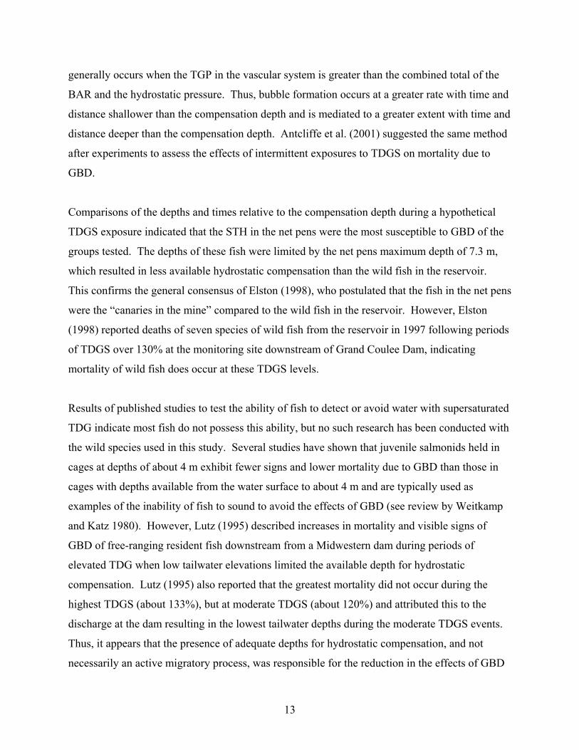
Comparisons of the depths and times relative to the compensation depth during a hypothetical
TDGS exposure indicated that the STH in the net pens were the most susceptible to GBD of the
groups tested. The depths of these fish were limited by the net pens maximum depth of 7.3 m,
which resulted in less available hydrostatic compensation than the wild fish in the reservoir.
This confirms the general consensus of Elston (1998), who postulated that the fish in the net pens
were the “canaries in the mine” compared to the wild fish in the reservoir. However, Elston
(1998) reported deaths of seven species of wild fish from the reservoir in 1997 following periods
of TDGS over 130% at the monitoring site downstream of Grand Coulee Dam, indicating
mortality of wild fish does occur at these TDGS levels.
Results of published studies to test the ability of fish to detect or avoid water with supersaturated
TDG indicate most fish do not possess this ability, but no such research has been conducted with
the wild species used in this study. Several studies have shown that juvenile salmonids held in
cages at depths of about 4 m exhibit fewer signs and lower mortality due to GBD than those in
cages with depths available from the water surface to about 4 m and are typically used as
examples of the inability of fish to sound to avoid the effects of GBD (see review by Weitkamp
and Katz 1980). However, Lutz (1995) described increases in mortality and visible signs of
GBD of free-ranging resident fish downstream from a Midwestern dam during periods of
elevated TDG when low tailwater elevations limited the available depth for hydrostatic
compensation. Lutz (1995) also reported that the greatest mortality did not occur during the
highest TDGS (about 133%), but at moderate TDGS (about 120%) and attributed this to the
discharge at the dam resulting in the lowest tailwater depths during the moderate TDGS events.
Thus, it appears that the presence of adequate depths for hydrostatic compensation, and not
necessarily an active migratory process, was responsible for the reduction in the effects of GBD
13

reported by Lutz (1995). This is a likely explanation of mortality due to GBD in other systems
as well, and would explain mortality of fish in areas known to have depths sufficient for
hydrostatic compensation. In this scenario, fish would not alter their depths in relation to TDGS
and their susceptibility to GBD would be related to the ambient TDGS, exposures to TDGS
based on species-specific depth histories (i.e., hydrostatic compensation), and species-specific
tolerances to TDGS.
It is not currently possible to accurately predict the true risk of GBD of a species even when
detailed depth data are available due to the lack of knowledge about the mechanism of
hydrostatic compensation and its function during intermittent exposures to TDGS. It is clear that
hydrostatic compensation can reduce the effects of GBD, but there is evidence that the effects are
due to more than the simple 9.6% of compensation per meter of depth that can be calculated
based on the increase in solubilities of gasses in liquids due to hydrostatic pressure. Knittle et
al. (1980) found that after previous exposure of juvenile steelhead to near-lethal levels of TDGS,
an exposure of 3-h to the hydrostatic compensation depth nearly doubled the time to 50%
mortality (LT50) during a subsequent surface exposure. They attributed this result to hydrostatic
pressure causing a resorption of gas emboli that had previously formed in the vasculature, but
this does not explain the entire effect, since the resulting LT50’s were greater than those of fish
with only a single surface exposure to TDGS. Fidler (1988) provided further information about
this effect via equations describing the dissolved gas thresholds required for formation of
bubbles in the vasculature system of rainbow trout (O. mykiss). These equations included total
gas pressure, partial pressure of oxygen, bubble nucleation site diameter and fish depth. Fidler
(1988) found that the TDG at which bubbles form within the vasculature was directly related to
fish depth and inversely related to the size of the bubble nucleation site. Aspen Applied Sciences
(1998) expanded on this work and noted an “additional protection” against GBD after fish were
exposed to depth, similar to the findings of Knittle et al. (1980). Aspen Applied Sciences (1998)
attributed this phenomenon to reductions in sizes of nucleation sites caused by the increased
pressure imparted by depth. However, there is currently no method of predicting the changes in
diameters of nucleation sites that occur during hydrostatic compensation, and thus, no method to
predict the probability of GBD during intermittent exposures to TDGS.
14

This study was conducted to assess the depths of fish relative to ambient TDG, but the ambient
TDG throughout the study was below levels generally shown to cause in-situ external GBD
symptoms and mortality of these species. Ryan et al. (2000) found few external signs of GBD in
resident fishes examined in the Columbia and Snake rivers between 1994 and 1997 when TDG
levels were less than 120%, nor was any mortality noted in fish held in net pens during these
conditions. However, the fact that fish kills are known to occur indicates that if fish do possess a
mechanism by which they can detect elevated TDG and “avoid”, or sound, to reduce the
subsequent effects of GBD, it is not a particularly effective system.
It is not clear whether maintaining a high tailwater below Grand Coulee Dam would reduce the
effects of TDGS on species that are shallow during periods of shallow tailwater elevations.
Maintaining a higher tailwater during this time period may increase the depths of resident fish,
particularly the WAL and LNS, between sunset and sunrise. However, whether this would
provide additional hydrostatic pressure or if the fish would move upward into shallow-water
habitats unavailable at lower tailwater elevations is not known. Maintaining higher tailwater
elevations could also result in greater TDGS generation during spill at Grand Coulee Dam by
increasing the depth of the plunge pool in the stilling basin, which may outweigh the benefit of a
potential increase in hydrostatic compensation.
Future research on the depths of resident fish using this method would be enhanced with the
addition of periodic estimates of the spatial locations of each test animal. These could be
provided by manually tracking an emitted radio signal by boat. The transmitters we used emitted
a radio signal to aid in their recapture only during short time windows to conserve battery life,
but the batteries on the archive tags are large relative to the tag deployment time and a radio
signal could have been emitted more often. This would allow a more detailed analysis of fish
movements relative to reservoir depth, TDG and tailwater elevation. For example, with the
current data it is not known if short forays to depths of approximately 20 m were from fish
moving along the bottom from one side of the reservoir to the other, or of fish in the middle of
the water column descending to a greater depth. Spatial location would also aid in determining
the relative importance of tailwater elevation on fish depths, since changes in tailwater elevations
diminish downstream due to the increasing cross-sectional volume of the reservoir.
15

In summary, the in-situ depths of triploid steelhead reared within a commercial net pen and
several species of wild resident fish in the reservoir were determined to assess their relative
exposures to TDGS downstream of Grand Coulee Dam on the Columbia River. Ambient TDGS
levels were low during the study period, but the relative differences in depths provided data with
which to assess their likely exposures to TDGS under simulated TDGS levels. Diel vertical
migrations were evident in all species, with changes occurring primarily near sunset and sunrise.
Most fish were deeper during the night than the day, but LNS and some WAL exhibited the
opposite behavior. The relative exposures to TDGS based on vertical distributions relative to a
standard TDGS level of 130%, in ascending order of severity, were LNS, LSS, WAL, BLS,
NPM and STH. Based on these results, the STH from the net pens would be expected to show
signs and mortality due to GBD prior to several of the resident species tested, though species-
specific tolerances to TDGS should also be considered.
16
References Antcliffe, B. L., L. E. Fidler, and I. K. Birtwell. In Press. Effects of dissolved gas
supersaturation on the survival and condition of juvenile rainbow trout (Oncorhynchus mykiss) under static and dynamic exposure scenarios. Canadian Technical Report of Fisheries and Aquatic Sciences.
Aspen Applied Sciences, Inc. 1998. Laboratory physiology studies for configuring and
calibrating the dynamic gas bubble trauma mortality model, final report. Prepared by Aspen Applied Sciences, Inc., Kalispell, Montana, for Battelle Pacific Northwest Division, contract DACW68-98-D-0002.
Backman, T. W. H., and A. E. Evans. 2002. Gas bubble trauma incidence in adult salmonids in
the Columbia River basin. North American Journal of Fisheries Management 22:579-584.
Beeman, J. W., P. V. Haner and A. G. Maule. 1998. Evaluation of a new miniature pressure-
sensitive radio transmitter. North American Journal of Fisheries Management 8:458-464. Beiningen, K. T. and W. J. Ebel. 1970. Effect of John Day Dam on dissolved nitrogen
concentrations and salmon in the Columbia River, 1968. Transactions of the American Fisheries Society 99:664-671.
Bouck, G. R. 1980. Etiology of gas bubble disease. Transactions of the American Fisheries
Society 109:703-707 Bouck, G. R., G. A. Chapman, P. W. Schneider, Jr., and D. G. Stevens. 1976. Observations on
gas bubble disease among wild adult Columbia River fishes. Transactions of the American Fisheries Society 105:114-115.
Colt, J. 1984. Computation of dissolved gas concentrations in water as functions of
temperature, salinity, and pressure. American Fisheries Society Special Publication 14. Crunkilton, R. L., J. M. Czarnezki, and L. Trial. 1980. Severe gas bubble disease in a
warmwater fishery in the Midwestern United States. Transactions of the American Fisheries Society 109:725-733.
Ebel, W. J., H. L. Raymond, G. E. Monan, W. E. Farr, and G. K. Tanonaka. 1975. Effect of
atmospheric gas supersaturation caused by dams on salmon and steelhead trout of the Snake and Columbia rivers. National Marine Fisheries Service, Northwest Fisheries Center, Seattle, Washington, USA.
Elston 1998. Fish kills in resident and captive fish caused by spill at Grand Coulee Dam in
1997: final report. Prepared by Aquatechnics Inc., Carlsborg, Washington for the Confederated Tribes of the Colville Reservation, Nespelem, Washington and Columbia River Fish Farms, Omak, Washington.
17

Elston, R., J. Colt, S. Abernethy, and W. A. Maslen. 1997. Bas bubble resorption in Chinook salmon: pressurization effects. Journal of Aquatic Animal Health 9:317-321.
Fidler, L. E. 1988. Gas bubble trauma in fish. Doctoral dissertation. University of British
Columbia. Frizell, K. H. 1996. Dissolved gas supersaturation study for Grand Coulee Dam Grand Coulee
Project, Washington. Prepared by the U.S. Bureau of Reclamation, Technical Service Center, Denver, Colorado, USA.
Frizell, K. H. and E. Cohen. 1998. Structural alternatives for TDG abatement at Grand Coulee
Dam: conceptual design report. Prepared by the U.S. Bureau of Reclamation, Technical Service Center, Denver, Colorado, USA
Hans, K. M., M. G. Mesa, and A. G. Maule. 1999. Rate of disappearance of gas bubble trauma
signs in juvenile salmonids. Journal of Aquatic Animal Health 11:383-390. Knittel, M. D., G. A. Chapman, and R. R. Garton. 1980. Effects of hydrostatic pressure on
steelhead survival in air-supersaturated water. Transactions of the American Fisheries Society 109:755-759.
Lutz, D. S. 1995. Gas supersaturation and gas bubble trauma in fish downstream from a
midwestern reservoir. Transactions of the American Fisheries Society 124:423-436. Mesa, M. G. and J. J. Warren. 1997. Predator avoidance ability of juvenile Chinook salmon
(Oncorhynchus tshawytscha) subjected to sublethal exposures of gas-supersaturated water. Canadian Journal of Fisheries and Aquatic Sciences 54:757-764.
Montgomery, J. C., and C. D. Becker. 1980. Gas bubble disease on smallmouth bass and
northern squawfish from the Snake and Columbia rivers. Transactions of the American Fisheries Society 109:734-736.
Ryan, B. A., E. M. Dawley, and R. A. Nelson. 2000. Modeling the effects of supersaturated
dissolved gas on resident aquatic biota in the main-stem Snake and Columbia rivers. North American Journal of Fisheries Management 20:92-204.
SAS (Statistical Analysis System). 1999. SAS Proprietary Software Release 8.1. Copyright
1999-2000 by SAS Institute Inc., Cary, North Carolina, USA. Venditti, D. A., T. C. Robinson, J. W. Beeman, B. J. Adams, and A. G. Maule. 2001. Gas
bubble disease in resident fish blow Grand Coulee Dam: 1999 annual report of research. Prepared by US Geological Survey, Cook Washington for US Bureau of Reclamation, Boise Idaho.
18

Weiland, L. K., M. M. Mesa, and A. G. Maule. 1999. Influence of infection with Renibacterium salmoninarum on susceptibility of juvenile spring Chinook salmon to gas bubble trauma. Journal of Aquatic Animal Health 11:123-129.
Weitkamp, D. E. and M. Katz. 1980. A review of dissolved gas supersaturation literature.
Transactions of the American Fisheries Society 109:659-702. Winter, J. D. 1983. Underwater biotelemetry. Pages 371-395 in L. A. Nielsen and D. L.
Johnson, editors. Fisheries techniques. American Fisheries Society, Bethesda, Maryland.
19
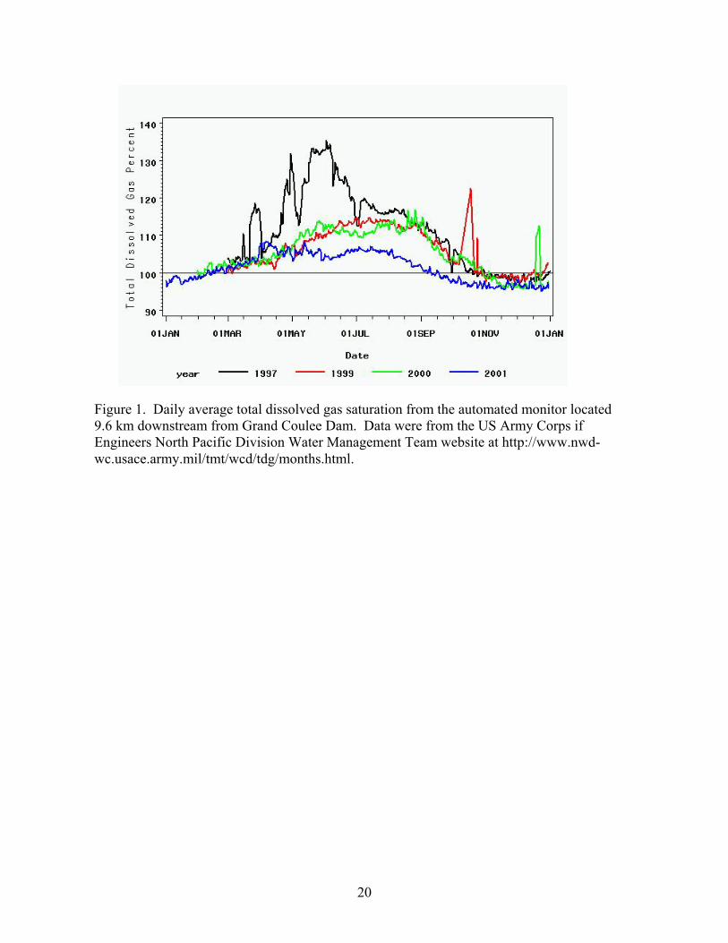
Figure 1. Daily average total dissolved gas saturation from the automated monitor located 9.6 km downstream from Grand Coulee Dam. Data were from the US Army Corps if Engineers North Pacific Division Water Management Team website at http://www.nwd-wc.usace.army.mil/tmt/wcd/tdg/months.html.
20

Figure 2. Median daily depths of wild bridgelip suckers (BLS), wild longnose suckers (LNS) and wild largescale suckers (LSS) from which archive tags were recovered during 2000 and 2001.
21

Figure 3. Median daily depths of wild northern pikeminnow (NPM), triploid steelhead reared at the Columbia River Fish Farm (STH) and wild walleye (WAL) from which archive tags were recovered during 2000 and 2001.
22
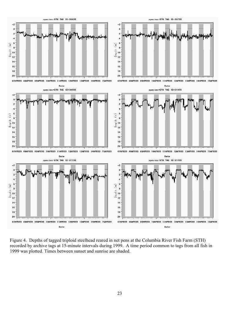
Figure 4. Depths of tagged triploid steelhead reared in net pens at the Columbia River Fish Farm (STH) recorded by archive tags at 15-minute intervals during 1999. A time period common to tags from all fish in 1999 was plotted. Times between sunset and sunrise are shaded.
23

Figure 5. Depths of bridgelip suckers (BLS) and northern pikeminnow (NPM) recorded at by archive tags 15-minute intervals during 2000. A time period common to tags from all fish in 2000 was plotted. Times between sunset and sunrise are shaded.
24

Figure 6. Depths of walleye (WAL) recorded at by archive tags 15-minute intervals during 2000. A time period common to tags from all fish in 2000 was plotted. Times between sunset and sunrise are shaded.
25

.
Figure 7. Depths of bridgelip suckers (BLS), longnose suckers (LNS) and largescale suckers (LSS) recorded at by archive tags 15-minute intervals during 2001. A time period common to tags from all fish in 2001 was plotted. Times between sunset and sunrise are shaded.
26

Figure 8. Depths of walleye (WAL) recorded by archive tags at 15-minute intervals during 2001. A time period common to tags from all fish in 2001 was plotted. Times between sunset and sunrise are shaded.
27
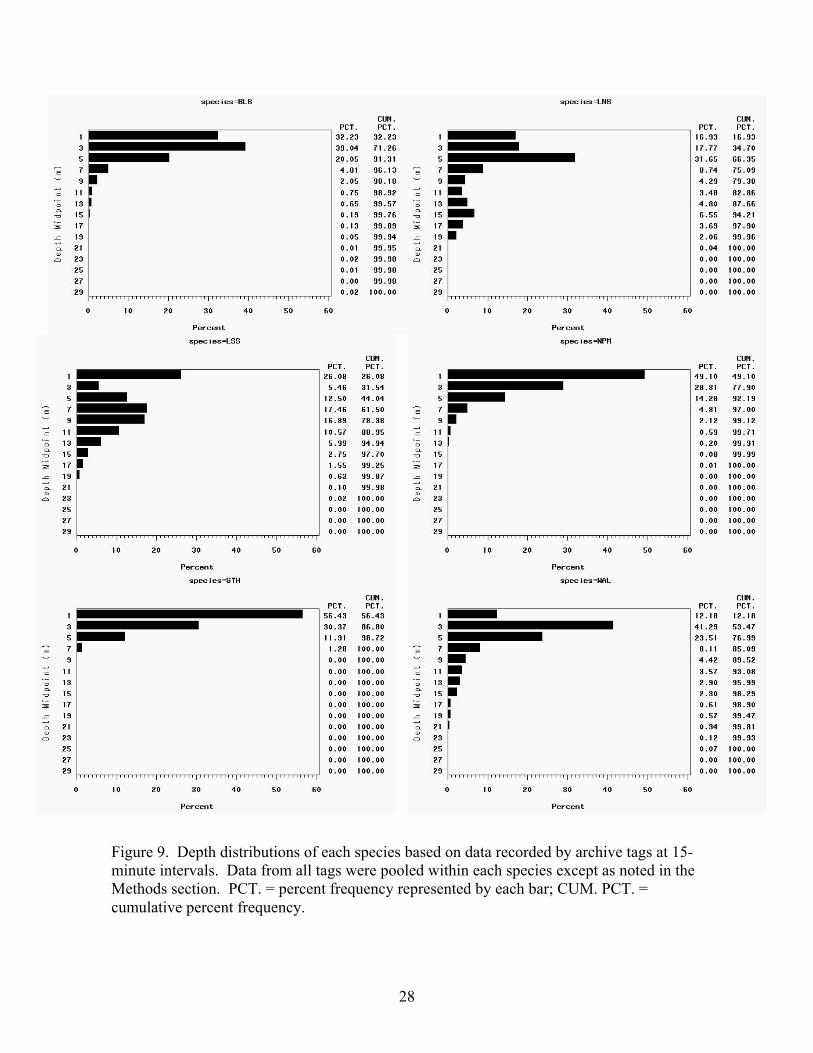
Figure 9. Depth distributions of each species based on data recorded by archive tags at 15-minute intervals. Data from all tags were pooled within each species except as noted in the Methods section. PCT. = percent frequency represented by each bar; CUM. PCT. = cumulative percent frequency.
28
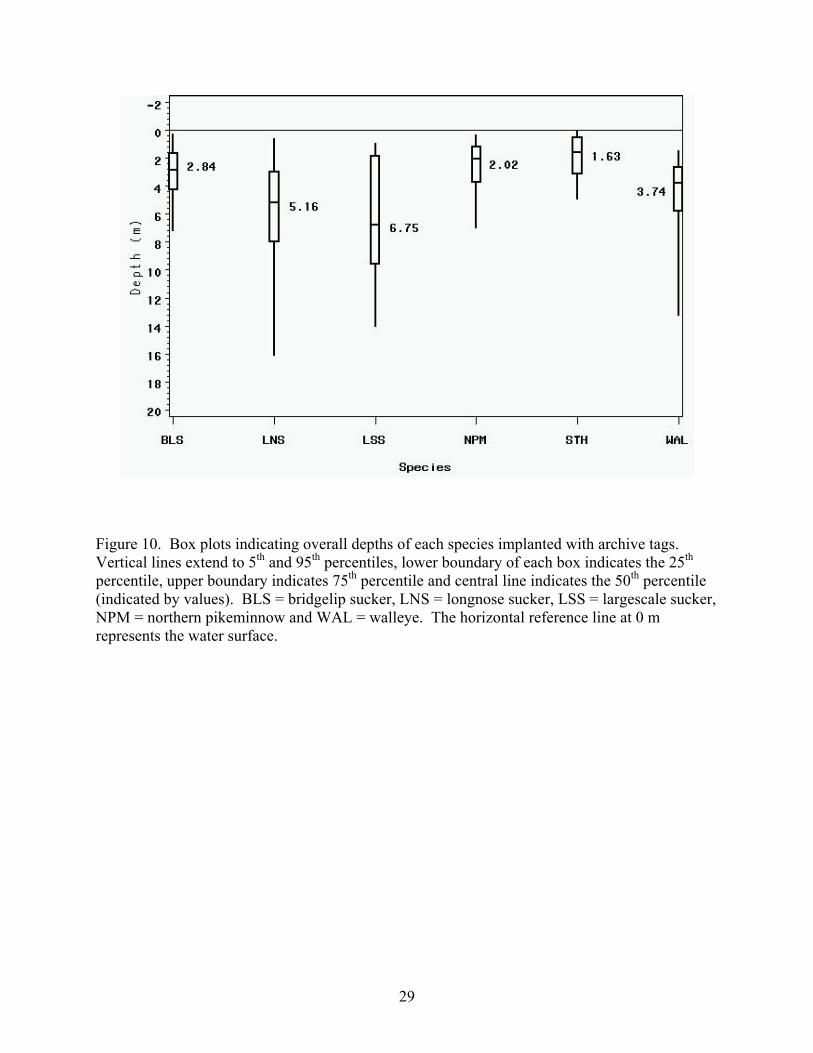
Figure 10. Box plots indicating overall depths of each species implanted with archive tags. Vertical lines extend to 5th and 95th percentiles, lower boundary of each box indicates the 25th percentile, upper boundary indicates 75th percentile and central line indicates the 50th percentile (indicated by values). BLS = bridgelip sucker, LNS = longnose sucker, LSS = largescale sucker, NPM = northern pikeminnow and WAL = walleye. The horizontal reference line at 0 m represents the water surface.
29

Figure 11. Box plots indicating depths of archive-tagged fish pooled by month. Vertical lines extend to 5th and 95th percentiles, lower boundary of each box indicates the 25th percentile, upper boundary indicates 75th percentile and central line indicates the 50th percentile (connected by lines). BLS = bridgelip sucker, LNS = longnose sucker, LSS = largescale sucker, NPM = northern pikeminnow and WAL = walleye. The horizontal reference line at 0 m represents the water surface.
30
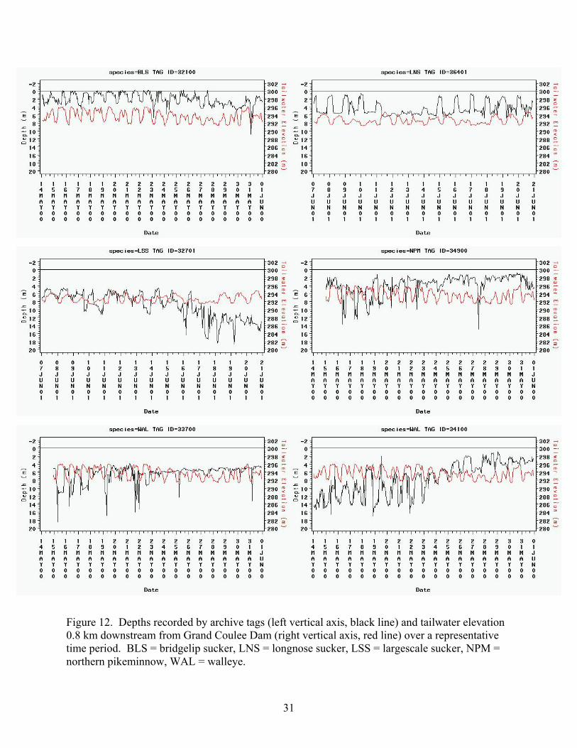
Figure 12. Depths recorded by archive tags (left vertical axis, black line) and tailwater elevation 0.8 km downstream from Grand Coulee Dam (right vertical axis, red line) over a representative time period. BLS = bridgelip sucker, LNS = longnose sucker, LSS = largescale sucker, NPM = northern pikeminnow, WAL = walleye.
31

Figure 13. Median distances and percent of data indicating archive-tagged fish would be above (upper plate) and at or below (lower plate) the hydrostatic compensation depth during an exposure to a hypothetical 130% TDGS.
32
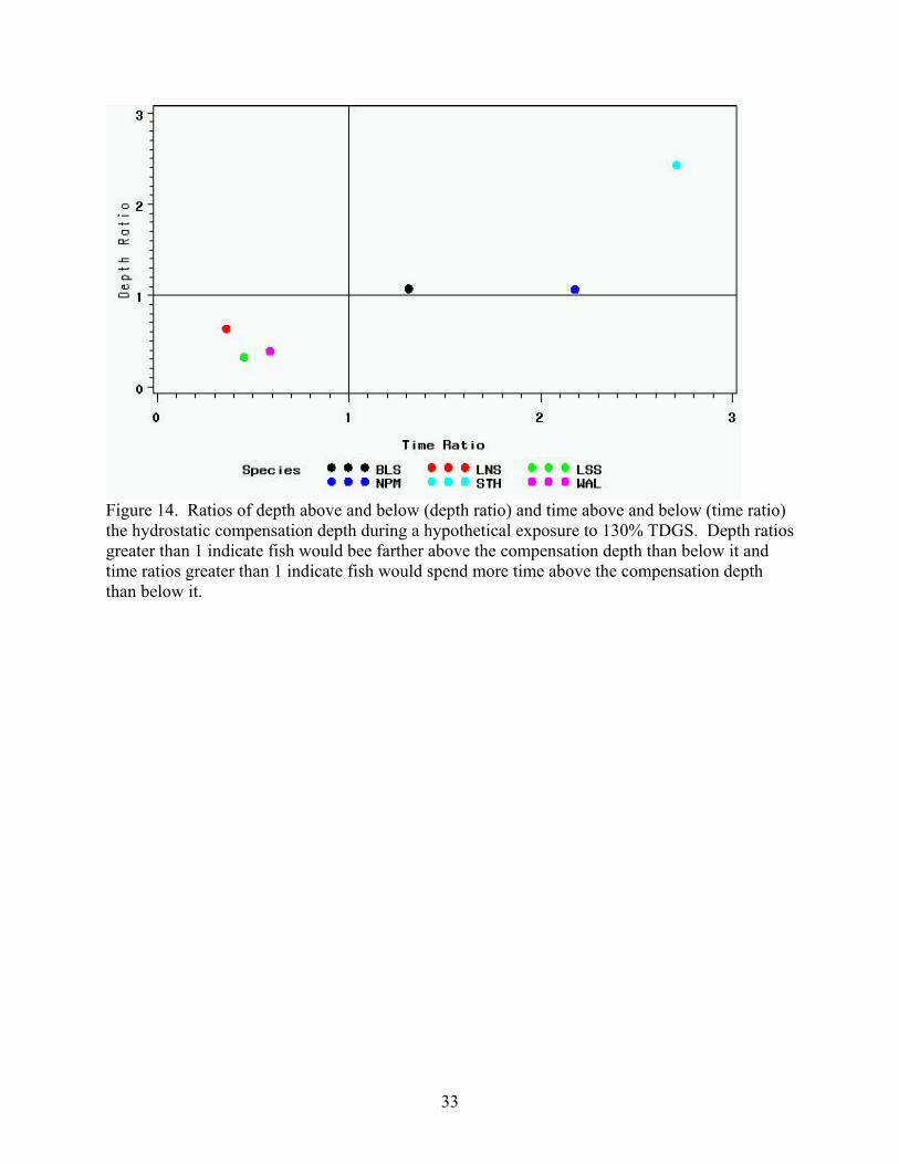
Figure 14. Ratios of depth above and below (depth ratio) and time above and below (time ratio) the hydrostatic compensation depth during a hypothetical exposure to 130% TDGS. Depth ratios greater than 1 indicate fish would bee farther above the compensation depth than below it and time ratios greater than 1 indicate fish would spend more time above the compensation depth than below it.
33
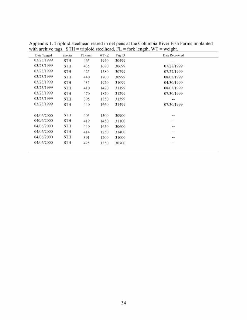
Appendix 1. Triploid steelhead reared in net pens at the Columbia River Fish Farms implanted with archive tags. STH = triploid steelhead, FL = fork length, WT = weight.
Date Tagged Species FL (mm) WT (g) Tag ID Date Recovered 03/23/1999 STH 465 1940 30499 -- 03/23/1999 STH 435 1680 30699 07/28/1999 03/23/1999 STH 425 1580 30799 07/27/1999 03/23/1999 STH 440 1700 30999 08/03/1999 03/23/1999 STH 435 1920 31099 04/30/1999 03/23/1999 STH 410 1420 31199 08/03/1999 03/23/1999 STH 470 1820 31299 07/30/1999 03/23/1999 STH 395 1350 31399 -- 03/23/1999 STH 440 1660 31499 07/30/1999
04/06/2000 STH 403 1300 30900 -- 040/6/2000 STH 419 1450 31100 -- 04/06/2000 STH 440 1650 30600 -- 04/06/2000 STH 414 1250 31400 -- 04/06/2000 STH 391 1200 31000 -- 04/06/2000 STH 425 1350 30700 --
34
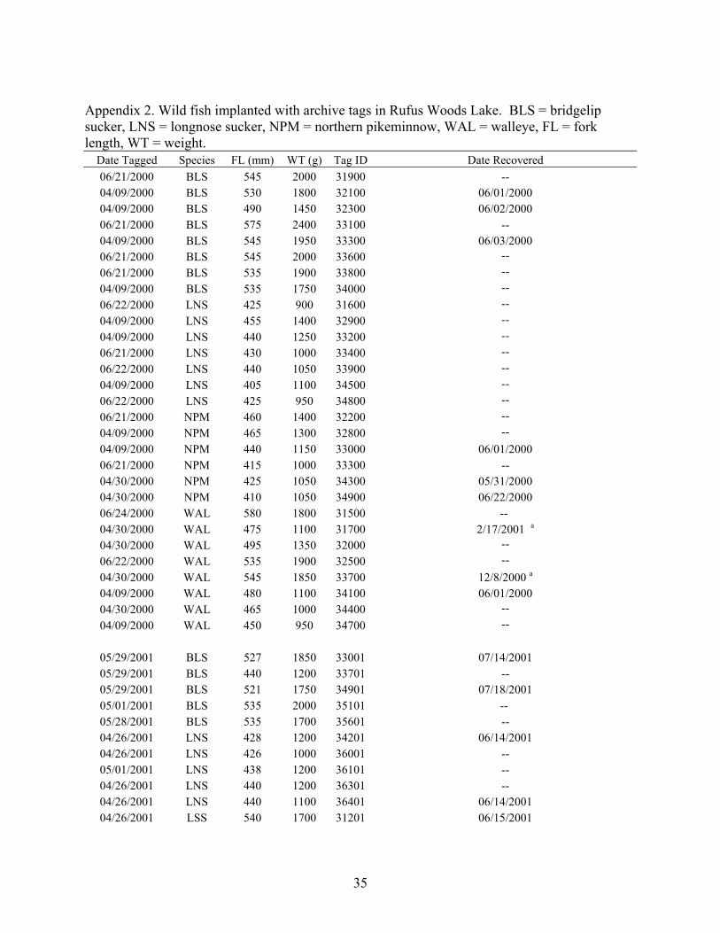
Appendix 2. Wild fish implanted with archive tags in Rufus Woods Lake. BLS = bridgelip sucker, LNS = longnose sucker, NPM = northern pikeminnow, WAL = walleye, FL = fork length, WT = weight.
Date Tagged Species FL (mm) WT (g) Tag ID Date Recovered 06/21/2000 BLS 545 2000 31900 -- 04/09/2000 BLS 530 1800 32100 06/01/2000 04/09/2000 BLS 490 1450 32300 06/02/2000 06/21/2000 BLS 575 2400 33100 -- 04/09/2000 BLS 545 1950 33300 06/03/2000 06/21/2000 BLS 545 2000 33600 -- 06/21/2000 BLS 535 1900 33800 -- 04/09/2000 BLS 535 1750 34000 -- 06/22/2000 LNS 425 900 31600 -- 04/09/2000 LNS 455 1400 32900 -- 04/09/2000 LNS 440 1250 33200 -- 06/21/2000 LNS 430 1000 33400 -- 06/22/2000 LNS 440 1050 33900 -- 04/09/2000 LNS 405 1100 34500 -- 06/22/2000 LNS 425 950 34800 -- 06/21/2000 NPM 460 1400 32200 -- 04/09/2000 NPM 465 1300 32800 -- 04/09/2000 NPM 440 1150 33000 06/01/2000 06/21/2000 NPM 415 1000 33300 -- 04/30/2000 NPM 425 1050 34300 05/31/2000 04/30/2000 NPM 410 1050 34900 06/22/2000 06/24/2000 WAL 580 1800 31500 -- 04/30/2000 WAL 475 1100 31700 2/17/2001 a
04/30/2000 WAL 495 1350 32000 -- 06/22/2000 WAL 535 1900 32500 -- 04/30/2000 WAL 545 1850 33700 12/8/2000 a
04/09/2000 WAL 480 1100 34100 06/01/2000 04/30/2000 WAL 465 1000 34400 -- 04/09/2000 WAL 450 950 34700 --
05/29/2001 BLS 527 1850 33001 07/14/2001 05/29/2001 BLS 440 1200 33701 -- 05/29/2001 BLS 521 1750 34901 07/18/2001 05/01/2001 BLS 535 2000 35101 -- 05/28/2001 BLS 535 1700 35601 -- 04/26/2001 LNS 428 1200 34201 06/14/2001 04/26/2001 LNS 426 1000 36001 -- 05/01/2001 LNS 438 1200 36101 -- 04/26/2001 LNS 440 1200 36301 -- 04/26/2001 LNS 440 1100 36401 06/14/2001 04/26/2001 LSS 540 1700 31201 06/15/2001
35
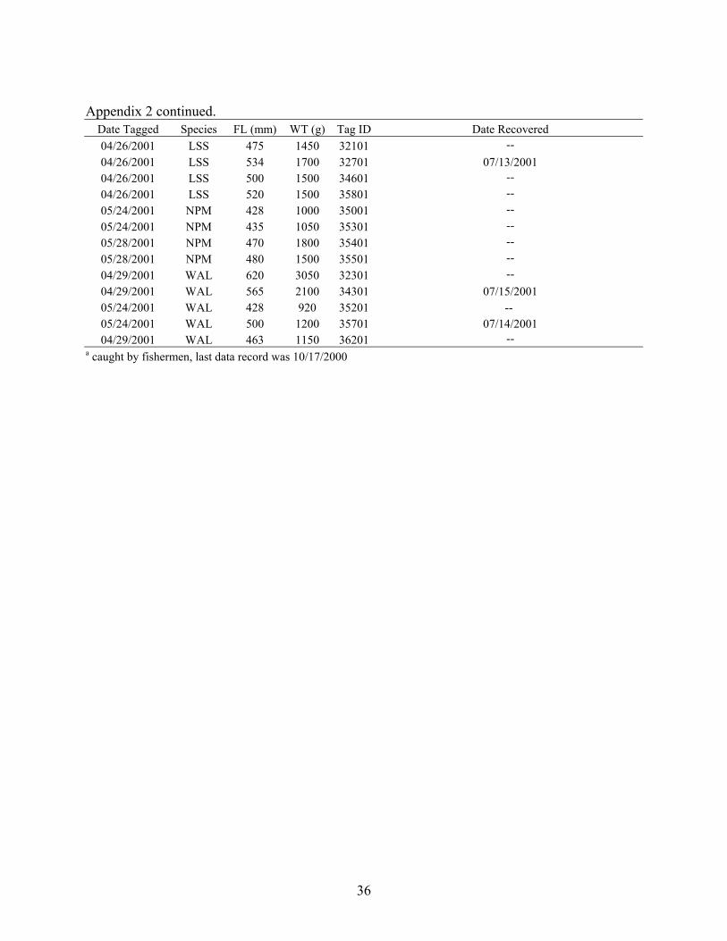
Appendix 2 continued.
Date Tagged Species FL (mm) WT (g) Tag ID Date Recovered 04/26/2001 LSS 475 1450 32101 -- 04/26/2001 LSS 534 1700 32701 07/13/2001 04/26/2001 LSS 500 1500 34601 -- 04/26/2001 LSS 520 1500 35801 -- 05/24/2001 NPM 428 1000 35001 -- 05/24/2001 NPM 435 1050 35301 -- 05/28/2001 NPM 470 1800 35401 -- 05/28/2001 NPM 480 1500 35501 -- 04/29/2001 WAL 620 3050 32301 -- 04/29/2001 WAL 565 2100 34301 07/15/2001 05/24/2001 WAL 428 920 35201 -- 05/24/2001 WAL 500 1200 35701 07/14/2001 04/29/2001 WAL 463 1150 36201 --
a caught by fishermen, last data record was 10/17/2000
36

Appendix 3. Monthly summaries of depth data (m) from archive tags implanted during 2000 and 2001. BLS = bridgelip sucker, LNS = longnose sucker, LSS = largescale sucker, NPM = northern pikeminnow, STH = triploid steelhead, WAL = walleye, Tag ID numbers ending in 00 are from 2000 and those ending in 01 are from 2001. Months are indicated by their numerical value (4 = April, 5 = May, etc.), N = sample size, Med = median, min= minimum, Max = maximum, CV = coefficient of variation, 5% = 5th percentile, 95% = 95th percentile, Wilk’s = Wilk’s lambda value for test of normality, Pr>W = probability of a larger Wilk’s lambda value (those ≤ 0.05 indicate a distribution with a significant deviation from normality). A value of . indicates no data. ________________________________________________________________________________________________________________ Species Tag ID Month N Mean Med Min Max Range CV 5% 95% Wilk's Pr>W ________________________________________________________________________________________________________________ BLS 32100 4 673 1.92 1.78 -0.25 6.89 7.14 60.78 0.39 4.12 0.9504 0.0000 5 2952 1.67 1.46 -0.25 20.25 20.50 80.83 -0.03 3.91 0.1021 0.0100 6 1 3.18 3.18 3.18 3.18 0.00 . 3.18 3.18 . . 32300 4 665 2.77 2.59 -0.31 15.46 15.77 77.78 0.04 6.65 0.9272 0.0000 5 2754 2.93 2.47 -0.31 22.31 22.62 75.55 -0.08 6.88 0.0967 0.0100 6 146 4.94 5.07 0.93 12.85 11.92 43.86 1.49 7.78 0.9417 0.0000 33001 6 1728 3.80 3.52 0.73 19.76 19.04 45.39 1.76 6.73 0.8603 0.0000 7 1252 4.31 3.52 0.31 19.76 19.45 60.41 1.55 9.11 0.8651 0.0000 33300 4 672 4.49 4.40 3.37 6.17 2.80 12.77 3.67 5.58 0.9699 0.0000 5 2976 3.56 3.37 -0.02 33.13 33.14 63.59 1.16 6.32 0.1355 0.0100 6 227 3.52 2.39 0.85 28.99 28.14 76.68 1.41 7.71 0.6738 0.0000 34901 6 1699 4.28 3.10 -0.25 15.69 15.94 87.59 0.25 12.58 0.8479 0.0000 7 1629 2.99 3.02 -0.25 15.19 15.44 56.61 0.42 5.79 0.9570 0.0000 Summary of BLS 4 2010 3.06 3.16 -0.31 15.46 15.77 58.89 0.39 5.84 0.0787 0.0100 5 8682 2.72 2.42 -0.31 33.13 33.44 78.55 0.07 6.17 0.0780 0.0100 6 3801 4.04 3.42 -0.25 28.99 29.25 71.50 0.67 10.82 0.1570 0.0100 7 2881 3.56 3.19 -0.25 19.76 20.02 62.70 0.73 8.59 0.1114 0.0100
37
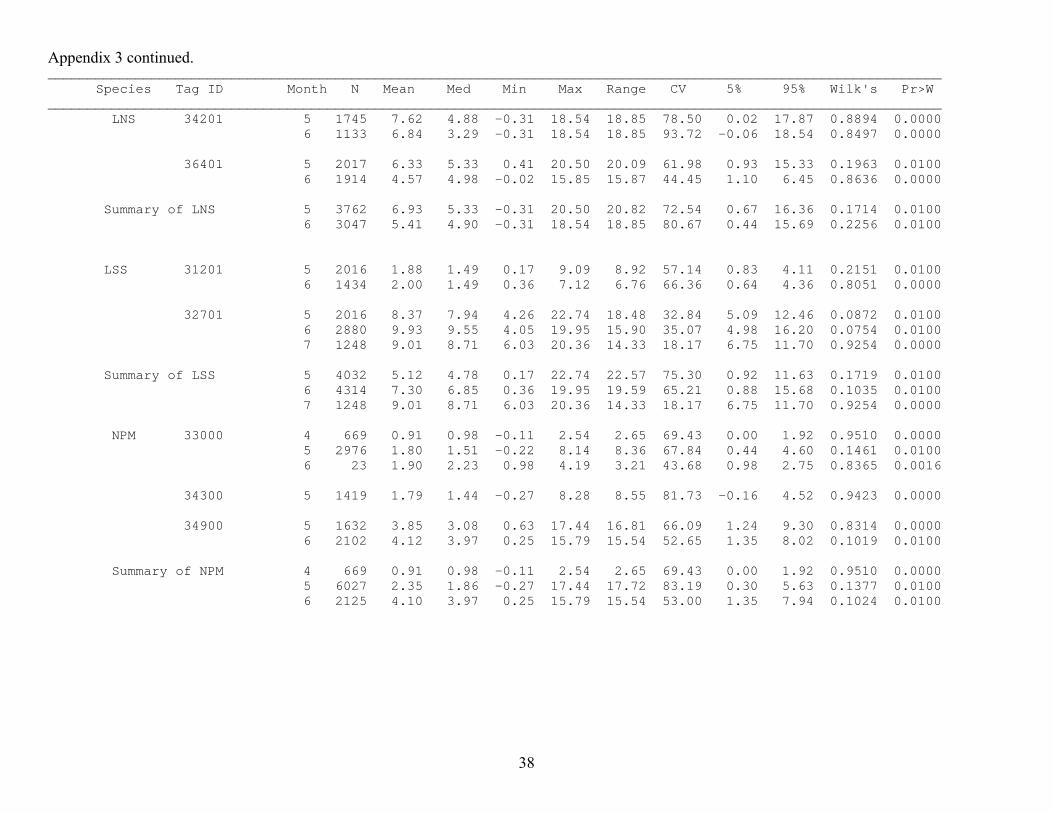
Appendix 3 continued. ________________________________________________________________________________________________________________ Species Tag ID Month N Mean Med Min Max Range CV 5% 95% Wilk's Pr>W ________________________________________________________________________________________________________________ LNS 34201 5 1745 7.62 4.88 -0.31 18.54 18.85 78.50 0.02 17.87 0.8894 0.0000 6 1133 6.84 3.29 -0.31 18.54 18.85 93.72 -0.06 18.54 0.8497 0.0000 36401 5 2017 6.33 5.33 0.41 20.50 20.09 61.98 0.93 15.33 0.1963 0.0100 6 1914 4.57 4.98 -0.02 15.85 15.87 44.45 1.10 6.45 0.8636 0.0000 Summary of LNS 5 3762 6.93 5.33 -0.31 20.50 20.82 72.54 0.67 16.36 0.1714 0.0100 6 3047 5.41 4.90 -0.31 18.54 18.85 80.67 0.44 15.69 0.2256 0.0100 LSS 31201 5 2016 1.88 1.49 0.17 9.09 8.92 57.14 0.83 4.11 0.2151 0.0100 6 1434 2.00 1.49 0.36 7.12 6.76 66.36 0.64 4.36 0.8051 0.0000 32701 5 2016 8.37 7.94 4.26 22.74 18.48 32.84 5.09 12.46 0.0872 0.0100 6 2880 9.93 9.55 4.05 19.95 15.90 35.07 4.98 16.20 0.0754 0.0100 7 1248 9.01 8.71 6.03 20.36 14.33 18.17 6.75 11.70 0.9254 0.0000 Summary of LSS 5 4032 5.12 4.78 0.17 22.74 22.57 75.30 0.92 11.63 0.1719 0.0100 6 4314 7.30 6.85 0.36 19.95 19.59 65.21 0.88 15.68 0.1035 0.0100 7 1248 9.01 8.71 6.03 20.36 14.33 18.17 6.75 11.70 0.9254 0.0000 NPM 33000 4 669 0.91 0.98 -0.11 2.54 2.65 69.43 0.00 1.92 0.9510 0.0000 5 2976 1.80 1.51 -0.22 8.14 8.36 67.84 0.44 4.60 0.1461 0.0100 6 23 1.90 2.23 0.98 4.19 3.21 43.68 0.98 2.75 0.8365 0.0016 34300 5 1419 1.79 1.44 -0.27 8.28 8.55 81.73 -0.16 4.52 0.9423 0.0000 34900 5 1632 3.85 3.08 0.63 17.44 16.81 66.09 1.24 9.30 0.8314 0.0000 6 2102 4.12 3.97 0.25 15.79 15.54 52.65 1.35 8.02 0.1019 0.0100 Summary of NPM 4 669 0.91 0.98 -0.11 2.54 2.65 69.43 0.00 1.92 0.9510 0.0000 5 6027 2.35 1.86 -0.27 17.44 17.72 83.19 0.30 5.63 0.1377 0.0100 6 2125 4.10 3.97 0.25 15.79 15.54 53.00 1.35 7.94 0.1024 0.0100
38
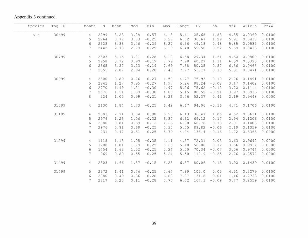
Appendix 3 continued. __________________________________________________________________________________________________________ __ Species Tag ID Month N Mean Med Min Max Range CV 5% 95% Wilk's Pr>W ________________________________________________________________________________________________________________ STH 30699 4 2299 3.23 3.28 0.57 6.18 5.61 25.68 1.83 4.55 0.0369 0.0100 5 2764 3.77 3.83 -0.25 6.27 6.52 36.67 1.29 5.91 0.0438 0.0100 6 2523 3.33 3.46 -0.29 6.27 6.56 49.18 0.48 5.85 0.0535 0.0100 7 2442 2.78 2.78 -0.29 6.19 6.48 59.50 0.22 5.68 0.0433 0.0100 30799 4 2303 3.15 3.21 -0.28 6.10 6.38 29.34 1.61 4.60 0.0800 0.0100 5 2958 3.92 3.90 -0.19 7.79 7.98 40.27 1.11 6.50 0.0393 0.0100 6 2865 3.37 3.23 -0.19 7.69 7.88 50.25 0.57 6.36 0.0468 0.0100 7 2555 2.87 2.94 -0.28 7.49 7.77 53.17 0.10 5.31 0.0471 0.0100 30999 4 2300 0.89 0.76 -0.27 4.50 4.77 75.93 0.10 2.26 0.1491 0.0100 5 2941 1.27 0.95 -0.27 4.97 5.24 88.24 -0.08 3.47 0.1402 0.0100 6 2770 1.49 1.21 -0.30 4.97 5.26 75.62 -0.12 3.70 0.1114 0.0100 7 2676 1.51 1.30 -0.30 4.85 5.15 80.52 -0.21 3.97 0.0936 0.0100 8 224 1.05 0.99 -0.21 3.26 3.46 52.37 0.41 2.19 0.9448 0.0000 31099 4 2130 1.84 1.73 -0.25 6.42 6.67 94.06 -0.16 4.71 0.1706 0.0100 31199 4 2303 2.94 3.04 0.08 6.20 6.13 36.47 1.06 4.62 0.0631 0.0100 5 2976 1.25 1.06 -0.32 6.30 6.62 69.12 0.17 2.94 0.1206 0.0100 6 2880 0.84 0.69 -0.12 4.26 4.38 68.78 0.13 2.01 0.1403 0.0100 7 2976 0.81 0.69 -0.25 5.30 5.55 89.82 -0.06 2.19 0.1059 0.0100 8 231 0.47 0.31 -0.25 3.79 4.04 133.4 -0.16 1.72 0.8363 0.0000 31299 4 1118 1.15 1.05 -0.25 4.11 4.37 72.31 0.03 2.63 0.9692 0.0000 5 1708 1.81 1.79 -0.25 5.23 5.48 56.08 0.12 3.56 0.9912 0.0000 6 1454 1.63 1.52 -0.25 5.24 5.50 70.34 -0.07 3.56 0.9744 0.0000 7 969 0.80 0.55 -0.25 5.24 5.50 119.9 -0.25 2.76 0.8572 0.0000 31499 4 2303 1.66 1.37 -0.15 6.23 6.37 80.06 0.15 3.90 0.1439 0.0100 31499 5 2972 1.41 0.76 -0.25 7.64 7.89 105.0 0.05 4.51 0.2279 0.0100 6 2880 0.49 0.36 -0.28 6.80 7.07 131.8 0.01 1.46 0.2733 0.0100 7 2817 0.23 0.11 -0.28 5.75 6.02 167.3 -0.09 0.77 0.2559 0.0100
39
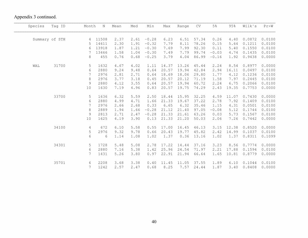
Appendix 3 continued. ________________________________________________________________________________________________________________ Species Tag ID Month N Mean Med Min Max Range CV 5% 95% Wilk's Pr>W ________________________________________________________________________________________________________________ Summary of STH 4 11508 2.37 2.61 -0.28 6.23 6.51 57.34 0.26 4.40 0.0872 0.0100 5 14611 2.30 1.91 -0.32 7.79 8.11 78.26 0.15 5.64 0.1211 0.0100 6 13918 1.87 1.21 -0.30 7.69 7.99 92.30 0.11 5.40 0.1550 0.0100 7 13466 1.58 1.04 -0.30 7.49 7.79 99.74 -0.03 4.74 0.1435 0.0100 8 455 0.76 0.68 -0.25 3.79 4.04 86.99 -0.16 1.92 0.9438 0.0000 WAL 31700 5 1632 4.67 4.02 1.11 14.37 13.26 45.44 2.24 8.54 0.8977 0.0000 6 2880 9.24 9.48 0.64 20.57 19.94 42.84 2.94 16.11 0.0497 0.0100 7 2976 2.81 2.71 0.64 18.69 18.06 29.80 1.77 4.12 0.1236 0.0100 8 2976 3.77 3.18 0.45 20.57 20.12 71.19 1.58 7.97 0.2445 0.0100 9 2880 4.12 3.55 0.64 20.57 19.94 60.72 2.24 6.75 0.2066 0.0100 10 1630 7.19 4.96 0.83 20.57 19.75 74.29 2.43 19.35 0.7753 0.0000 33700 5 1636 6.32 5.59 2.50 18.44 15.95 32.25 4.59 11.07 0.7430 0.0000 6 2880 4.99 4.71 1.66 21.33 19.67 37.22 2.78 7.92 0.1409 0.0100 7 2976 2.66 2.68 0.33 6.65 6.32 35.46 1.15 4.31 0.0501 0.0100 8 2889 1.94 1.66 -0.28 21.12 21.40 97.05 -0.08 5.12 0.1744 0.0100 9 2813 2.71 2.47 -0.28 21.33 21.61 63.26 0.03 5.73 0.1567 0.0100 10 1625 4.19 3.90 0.13 21.33 21.20 50.03 2.06 7.26 0.7442 0.0000 34100 4 672 6.10 5.58 0.55 17.00 16.45 46.13 3.15 12.38 0.8520 0.0000 5 2976 9.32 9.78 0.66 20.43 19.77 45.82 2.42 14.99 0.1037 0.0100 6 6 1.14 1.08 1.02 1.37 0.36 13.16 1.02 1.37 0.8311 0.1099 34301 5 1728 5.48 5.08 2.78 17.22 14.44 37.16 3.23 8.56 0.7774 0.0000 6 2880 7.16 5.38 1.42 25.96 24.54 71.97 2.21 17.88 0.1594 0.0100 7 1431 5.26 3.80 0.97 22.91 21.94 66.64 1.65 10.81 0.8779 0.0000 35701 6 2208 3.68 3.38 0.40 11.45 11.05 37.55 1.89 6.10 0.1044 0.0100 7 1242 2.57 2.47 0.68 8.25 7.57 24.44 1.87 3.40 0.8408 0.0000
40

Appendix 3 continued. ________________________________________________________________________________________________________________ Species Tag ID Month N Mean Med Min Max Range CV 5% 95% Wilk's Pr>W ________________________________________________________________________________________________________________ Summary of WAL 4 672 6.10 5.58 0.55 17.00 16.45 46.13 3.15 12.38 0.8520 0.0000 5 7972 6.92 5.64 0.66 20.43 19.77 52.50 2.71 14.28 0.1643 0.0100 6 10854 6.43 5.13 0.40 25.96 25.57 63.90 2.27 14.99 0.1581 0.0100 7 8625 3.13 2.71 0.33 22.91 22.58 60.21 1.45 7.87 0.2199 0.0100 8 5865 2.87 2.52 -0.28 21.12 21.40 87.05 0.23 6.09 0.1677 0.0100 9 5693 3.42 3.08 -0.28 21.33 21.61 66.11 1.15 6.19 0.1465 0.0100 10 3255 5.69 4.20 0.13 21.33 21.20 76.03 2.27 16.44 0.2604 0.0100 ________________________________________________________________________________________________________________
41
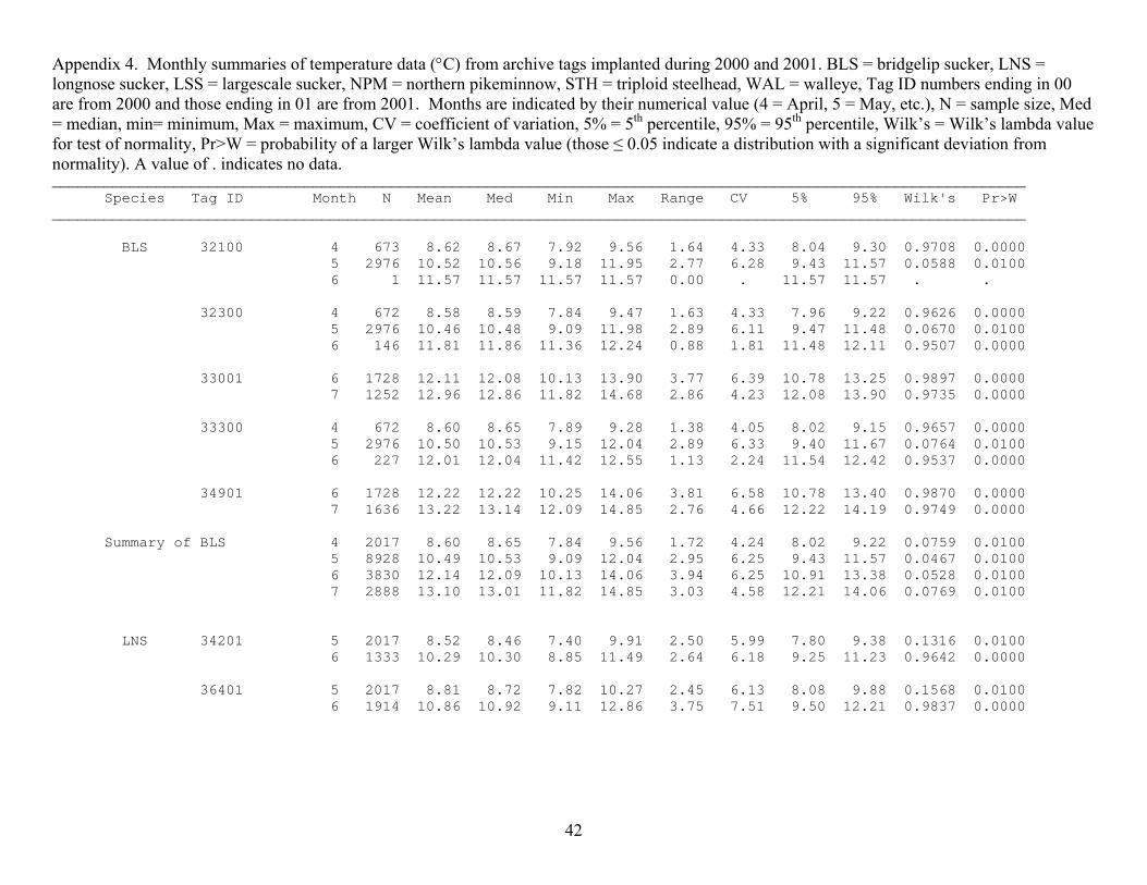
Appendix 4. Monthly summaries of temperature data (°C) from archive tags implanted during 2000 and 2001. BLS = bridgelip sucker, LNS = longnose sucker, LSS = largescale sucker, NPM = northern pikeminnow, STH = triploid steelhead, WAL = walleye, Tag ID numbers ending in 00 are from 2000 and those ending in 01 are from 2001. Months are indicated by their numerical value (4 = April, 5 = May, etc.), N = sample size, Med = median, min= minimum, Max = maximum, CV = coefficient of variation, 5% = 5th percentile, 95% = 95th percentile, Wilk’s = Wilk’s lambda value for test of normality, Pr>W = probability of a larger Wilk’s lambda value (those ≤ 0.05 indicate a distribution with a significant deviation from normality). A value of . indicates no data. ________________________________________________________________________________________________________________ Species Tag ID Month N Mean Med Min Max Range CV 5% 95% Wilk's Pr>W ________________________________________________________________________________________________________________ BLS 32100 4 673 8.62 8.67 7.92 9.56 1.64 4.33 8.04 9.30 0.9708 0.0000 5 2976 10.52 10.56 9.18 11.95 2.77 6.28 9.43 11.57 0.0588 0.0100 6 1 11.57 11.57 11.57 11.57 0.00 . 11.57 11.57 . . 32300 4 672 8.58 8.59 7.84 9.47 1.63 4.33 7.96 9.22 0.9626 0.0000 5 2976 10.46 10.48 9.09 11.98 2.89 6.11 9.47 11.48 0.0670 0.0100 6 146 11.81 11.86 11.36 12.24 0.88 1.81 11.48 12.11 0.9507 0.0000 33001 6 1728 12.11 12.08 10.13 13.90 3.77 6.39 10.78 13.25 0.9897 0.0000 7 1252 12.96 12.86 11.82 14.68 2.86 4.23 12.08 13.90 0.9735 0.0000 33300 4 672 8.60 8.65 7.89 9.28 1.38 4.05 8.02 9.15 0.9657 0.0000 5 2976 10.50 10.53 9.15 12.04 2.89 6.33 9.40 11.67 0.0764 0.0100 6 227 12.01 12.04 11.42 12.55 1.13 2.24 11.54 12.42 0.9537 0.0000 34901 6 1728 12.22 12.22 10.25 14.06 3.81 6.58 10.78 13.40 0.9870 0.0000 7 1636 13.22 13.14 12.09 14.85 2.76 4.66 12.22 14.19 0.9749 0.0000
Summary of BLS 4 2017 8.60 8.65 7.84 9.56 1.72 4.24 8.02 9.22 0.0759 0.0100 5 8928 10.49 10.53 9.09 12.04 2.95 6.25 9.43 11.57 0.0467 0.0100 6 3830 12.14 12.09 10.13 14.06 3.94 6.25 10.91 13.38 0.0528 0.0100 7 2888 13.10 13.01 11.82 14.85 3.03 4.58 12.21 14.06 0.0769 0.0100 LNS 34201 5 2017 8.52 8.46 7.40 9.91 2.50 5.99 7.80 9.38 0.1316 0.0100 6 1333 10.29 10.30 8.85 11.49 2.64 6.18 9.25 11.23 0.9642 0.0000 36401 5 2017 8.81 8.72 7.82 10.27 2.45 6.13 8.08 9.88 0.1568 0.0100 6 1914 10.86 10.92 9.11 12.86 3.75 7.51 9.50 12.21 0.9837 0.0000
42

Appendix 4 continued. ________________________________________________________________________________________________________________ Species Tag ID Month N Mean Med Min Max Range CV 5% 95% Wilk's Pr>W ________________________________________________________________________________________________________________
Summary of LNS 5 4034 8.66 8.59 7.40 10.27 2.87 6.29 7.93 9.63 0.1123 0.0100 6 3247 10.63 10.66 8.85 12.86 4.00 7.51 9.38 11.95 0.0566 0.0100 LSS 31201 5 2016 9.22 9.10 7.79 10.67 2.87 5.96 8.44 10.14 0.0943 0.0100 6 1434 10.96 10.93 9.36 12.63 3.27 6.46 9.88 11.97 0.9638 0.0000 32701 5 2016 8.52 8.36 7.31 9.93 2.62 6.39 7.84 9.41 0.1294 0.0100 6 2880 10.89 10.98 8.62 13.08 4.46 8.64 9.41 12.42 0.0626 0.0100 7 1248 12.44 12.42 11.24 13.73 2.49 3.55 11.77 13.21 0.9844 0.0000
Summary of LSS 5 4032 8.87 8.84 7.31 10.67 3.35 7.33 7.92 10.01 0.0578 0.0100 6 4314 10.91 10.98 8.62 13.08 4.46 7.98 9.54 12.29 0.0516 0.0100 7 1248 12.44 12.42 11.24 13.73 2.49 3.55 11.77 13.21 0.9844 0.0000 NPM 33000 4 672 10.17 9.87 7.49 13.63 6.14 12.17 8.49 12.38 0.9697 0.0000 5 2976 11.35 11.12 8.49 17.26 8.77 12.04 9.74 14.25 0.1594 0.0100 6 24 10.27 11.75 7.61 12.25 4.64 18.78 7.74 12.25 0.7297 0.0000 34300 5 1542 11.15 10.61 9.69 18.28 8.59 13.80 9.82 14.71 0.7549 0.0000 34900 5 1632 10.39 10.30 9.64 11.61 1.97 4.13 9.77 11.08 0.9407 0.0000 6 2102 12.26 12.26 10.82 13.97 3.15 4.20 11.35 13.05 0.0873 0.0100
Summary of NPM 4 672 10.17 9.87 7.49 13.63 6.14 12.17 8.49 12.38 0.9697 0.0000 5 6150 11.04 10.69 8.49 18.28 9.79 11.83 9.82 13.92 0.1832 0.0100 6 2126 12.24 12.26 7.61 13.97 6.36 4.81 11.35 13.05 0.1079 0.0100 STH 30699 4 2303 6.28 6.25 5.00 7.98 2.98 12.08 5.13 7.73 0.0853 0.0100 5 2976 9.22 9.35 7.73 10.73 3.00 7.34 7.98 10.23 0.1628 0.0100 6 2880 12.62 12.98 10.35 13.98 3.63 7.69 10.73 13.85 0.1624 0.0100 7 2660 14.72 14.73 13.60 16.10 2.50 3.74 13.85 15.60 0.0955 0.0100 30799 4 2303 6.41 6.38 5.13 8.10 2.98 12.15 5.25 7.85 0.1007 0.0100 5 2976 9.29 9.35 7.73 10.73 3.00 7.20 7.98 10.35 0.1569 0.0100 6 2880 12.61 12.85 10.48 13.85 3.38 6.90 10.91 13.73 0.1350 0.0100 7 2558 14.63 14.60 13.60 16.35 2.75 3.61 13.85 15.48 0.1028 0.0100 30999 4 2303 6.78 6.88 5.50 8.23 2.73 9.79 5.75 7.85 0.0763 0.0100 5 2976 9.37 9.48 7.98 11.10 3.13 7.00 8.23 10.35 0.1650 0.0100 6 2880 12.74 12.98 10.48 14.35 3.88 7.49 10.85 13.85 0.1581 0.0100 7 2976 14.94 14.98 13.73 16.35 2.63 4.00 13.98 15.85 0.1025 0.0100 8 228 16.01 15.98 15.60 16.48 0.88 1.57 15.73 16.35 0.8935 0.0000
43

Appendix 4 continued. ________________________________________________________________________________________________________________ Species Tag ID Month N Mean Med Min Max Range CV 5% 95% Wilk's Pr>W ________________________________________________________________________________________________________________ STH 31099 4 2143 6.30 6.25 5.00 8.35 3.35 11.37 5.25 7.48 0.1192 0.0100 31199 4 2303 6.41 6.38 5.13 8.23 3.10 11.95 5.25 7.73 0.0933 0.0100 5 2976 9.29 9.48 7.85 10.85 3.00 7.34 8.10 10.35 0.1586 0.0100 6 2880 12.68 12.98 10.48 14.35 3.88 7.38 10.85 13.85 0.1463 0.0100 7 2976 14.87 14.98 13.73 15.98 2.25 3.96 13.98 15.73 0.1007 0.0100 8 231 15.93 15.98 15.48 16.35 0.88 1.51 15.60 16.35 0.9299 0.0000 31299 4 2303 6.29 6.38 5.00 7.98 2.98 11.33 5.25 7.60 0.0815 0.0100 5 2976 9.17 9.35 7.73 10.73 3.00 7.14 7.98 10.10 0.1475 0.0100 6 2880 12.59 12.85 10.35 14.10 3.75 8.01 10.73 13.85 0.1643 0.0100 7 2818 14.79 14.85 13.60 15.98 2.38 3.90 13.85 15.73 0.0934 0.0100 31499 4 2303 6.35 6.38 5.00 7.98 2.98 11.93 5.25 7.60 0.0802 0.0100 5 2976 9.20 9.35 7.73 10.73 3.00 7.29 7.98 10.23 0.1694 0.0100 6 2880 12.65 12.98 10.35 13.98 3.63 7.81 10.73 13.85 0.1540 0.0100 7 2817 14.86 14.85 13.60 16.10 2.50 3.98 13.85 15.73 0.1048 0.0100
Summary of STH 4 11515 6.45 6.38 5.00 8.23 3.23 11.88 5.25 7.73 0.0744 0.0100 5 14880 9.28 9.48 7.73 11.10 3.38 7.26 7.98 10.23 0.1547 0.0100 6 14400 12.66 12.98 10.35 14.35 4.00 7.47 10.85 13.85 0.1507 0.0100 7 13987 14.81 14.85 13.60 16.35 2.75 3.95 13.85 15.73 0.0858 0.0100 8 459 15.97 15.98 15.48 16.48 1.00 1.56 15.60 16.35 0.9279 0.0000 WAL 31700 5 1632 10.07 9.91 9.25 14.55 5.30 7.16 9.38 10.97 0.7434 0.0000 6 2880 12.10 12.03 10.04 17.47 7.42 6.62 10.97 13.62 0.0936 0.0100 7 2976 14.76 14.81 12.29 19.06 6.76 7.15 12.96 16.40 0.0635 0.0100 8 2976 17.25 17.33 15.48 19.06 3.58 3.28 16.14 18.00 0.1270 0.0100 9 2880 17.39 17.60 12.96 18.39 5.44 3.57 16.40 18.00 0.1473 0.0100 10 1630 15.34 15.34 12.82 16.67 3.85 4.16 14.28 16.40 0.9625 0.0000
44
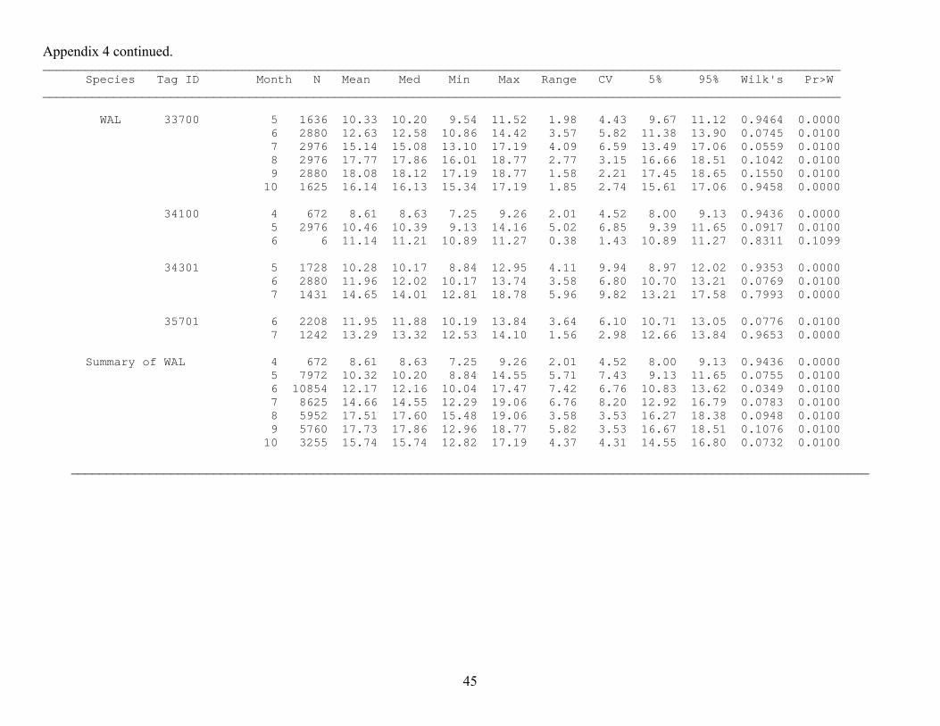
Appendix 4 continued. ________________________________________________________________________________________________________________ Species Tag ID Month N Mean Med Min Max Range CV 5% 95% Wilk's Pr>W ________________________________________________________________________________________________________________ WAL 33700 5 1636 10.33 10.20 9.54 11.52 1.98 4.43 9.67 11.12 0.9464 0.0000 6 2880 12.63 12.58 10.86 14.42 3.57 5.82 11.38 13.90 0.0745 0.0100 7 2976 15.14 15.08 13.10 17.19 4.09 6.59 13.49 17.06 0.0559 0.0100 8 2976 17.77 17.86 16.01 18.77 2.77 3.15 16.66 18.51 0.1042 0.0100 9 2880 18.08 18.12 17.19 18.77 1.58 2.21 17.45 18.65 0.1550 0.0100 10 1625 16.14 16.13 15.34 17.19 1.85 2.74 15.61 17.06 0.9458 0.0000 34100 4 672 8.61 8.63 7.25 9.26 2.01 4.52 8.00 9.13 0.9436 0.0000 5 2976 10.46 10.39 9.13 14.16 5.02 6.85 9.39 11.65 0.0917 0.0100 6 6 11.14 11.21 10.89 11.27 0.38 1.43 10.89 11.27 0.8311 0.1099 34301 5 1728 10.28 10.17 8.84 12.95 4.11 9.94 8.97 12.02 0.9353 0.0000 6 2880 11.96 12.02 10.17 13.74 3.58 6.80 10.70 13.21 0.0769 0.0100 7 1431 14.65 14.01 12.81 18.78 5.96 9.82 13.21 17.58 0.7993 0.0000 35701 6 2208 11.95 11.88 10.19 13.84 3.64 6.10 10.71 13.05 0.0776 0.0100 7 1242 13.29 13.32 12.53 14.10 1.56 2.98 12.66 13.84 0.9653 0.0000
Summary of WAL 4 672 8.61 8.63 7.25 9.26 2.01 4.52 8.00 9.13 0.9436 0.0000 5 7972 10.32 10.20 8.84 14.55 5.71 7.43 9.13 11.65 0.0755 0.0100 6 10854 12.17 12.16 10.04 17.47 7.42 6.76 10.83 13.62 0.0349 0.0100 7 8625 14.66 14.55 12.29 19.06 6.76 8.20 12.92 16.79 0.0783 0.0100 8 5952 17.51 17.60 15.48 19.06 3.58 3.53 16.27 18.38 0.0948 0.0100 9 5760 17.73 17.86 12.96 18.77 5.82 3.53 16.67 18.51 0.1076 0.0100 10 3255 15.74 15.74 12.82 17.19 4.37 4.31 14.55 16.80 0.0732 0.0100 ________________________________________________________________________________________________________________
45
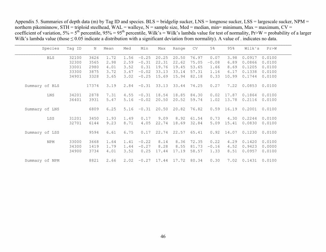
Appendix 5. Summaries of depth data (m) by Tag ID and species. BLS = bridgelip sucker, LNS = longnose sucker, LSS = largescale sucker, NPM = northern pikeminnow, STH = triploid steelhead, WAL = walleye, N = sample size, Med = median, min= minimum, Max = maximum, CV = coefficient of variation, 5% = 5th percentile, 95% = 95th percentile, Wilk’s = Wilk’s lambda value for test of normality, Pr>W = probability of a larger Wilk’s lambda value (those ≤ 0.05 indicate a distribution with a significant deviation from normality). A value of . indicates no data. ________________________________________________________________________________________________________________ Species Tag ID N Mean Med Min Max Range CV 5% 95% Wilk's Pr>W ________________________________________________________________________________________________________________ BLS 32100 3626 1.72 1.56 -0.25 20.25 20.50 76.97 0.07 3.98 0.0917 0.0100 32300 3565 2.98 2.59 -0.31 22.31 22.62 75.05 -0.08 6.89 0.0866 0.0100 33001 2980 4.01 3.52 0.31 19.76 19.45 53.65 1.66 8.69 0.1205 0.0100 33300 3875 3.72 3.67 -0.02 33.13 33.14 57.31 1.16 6.17 0.1338 0.0100 34901 3328 3.65 3.02 -0.25 15.69 15.94 82.18 0.33 10.99 0.1744 0.0100 Summary of BLS 17374 3.19 2.84 -0.31 33.13 33.44 74.25 0.27 7.22 0.0853 0.0100 LNS 34201 2878 7.31 4.55 -0.31 18.54 18.85 84.30 0.02 17.87 0.1864 0.0100 36401 3931 5.47 5.16 -0.02 20.50 20.52 59.74 1.02 13.78 0.2116 0.0100 Summary of LNS 6809 6.25 5.16 -0.31 20.50 20.82 76.82 0.59 16.19 0.2001 0.0100 LSS 31201 3450 1.93 1.49 0.17 9.09 8.92 61.54 0.73 4.30 0.2244 0.0100 32701 6144 9.23 8.71 4.05 22.74 18.69 32.84 5.09 15.41 0.0830 0.0100 Summary of LSS 9594 6.61 6.75 0.17 22.74 22.57 65.41 0.92 14.07 0.1230 0.0100 NPM 33000 3668 1.64 1.41 -0.22 8.14 8.36 72.35 0.22 4.29 0.1420 0.0100 34300 1419 1.79 1.44 -0.27 8.28 8.55 81.73 -0.16 4.52 0.9423 0.0000 34900 3734 4.01 3.52 0.25 17.44 17.19 58.57 1.33 8.51 0.0957 0.0100 Summary of NPM 8821 2.66 2.02 -0.27 17.44 17.72 80.34 0.30 7.02 0.1431 0.0100
46

Appendix 5 continued. ________________________________________________________________________________________________________________ Species Tag ID N Mean Med Min Max Range CV 5% 95% Wilk's Pr>W ________________________________________________________________________________________________________________ STH 30699 10028 3.29 3.37 -0.29 6.27 6.56 44.54 0.65 5.73 0.0353 0.0100 30799 10681 3.35 3.31 -0.28 7.79 8.08 45.72 0.61 6.00 0.0392 0.0100 30999 10911 1.30 1.04 -0.30 4.97 5.26 83.57 -0.03 3.52 0.1253 0.0100 31099 2130 1.84 1.73 -0.25 6.42 6.67 94.06 -0.16 4.71 0.1706 0.0100 31199 11366 1.36 0.97 -0.32 6.30 6.62 85.08 0.03 3.83 0.1492 0.0100 31299 5249 1.43 1.33 -0.25 5.24 5.50 75.26 -0.07 3.37 0.0608 0.0100 31499 10972 0.92 0.39 -0.28 7.64 7.92 131.5 0.01 3.70 0.2637 0.0100 Summary of STH 53958 2.01 1.63 -0.32 7.79 8.11 82.87 0.05 5.10 0.1230 0.0100 WAL 31700 14974 5.17 3.65 0.45 20.57 20.12 74.28 1.96 13.62 0.2244 0.0100 33700 14819 3.55 3.19 -0.28 21.33 21.61 63.75 0.54 6.78 0.0744 0.0100 34100 3654 8.72 8.36 0.55 20.43 19.89 48.63 2.53 14.87 0.1142 0.0100 34301 6039 6.23 5.08 0.97 25.96 24.99 67.27 1.99 15.67 0.1446 0.0100 35701 3450 3.28 2.85 0.40 11.45 11.05 39.18 1.87 5.84 0.1496 0.0100 Summary of WAL 42936 4.91 3.74 -0.28 25.96 26.24 74.54 1.42 13.33 0.1661 0.0100 ________________________________________________________________________________________________________________
47
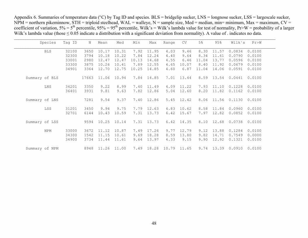
Appendix 6. Summaries of temperature data (°C) by Tag ID and species. BLS = bridgelip sucker, LNS = longnose sucker, LSS = largescale sucker, NPM = northern pikeminnow, STH = triploid steelhead, WAL = walleye, N = sample size, Med = median, min= minimum, Max = maximum, CV = coefficient of variation, 5% = 5th percentile, 95% = 95th percentile, Wilk’s = Wilk’s lambda value for test of normality, Pr>W = probability of a larger Wilk’s lambda value (those ≤ 0.05 indicate a distribution with a significant deviation from normality). A value of . indicates no data. ________________________________________________________________________________________________________________ Species Tag ID N Mean Med Min Max Range CV 5% 95% Wilk's Pr>W ________________________________________________________________________________________________________________ BLS 32100 3650 10.17 10.31 7.92 11.95 4.03 9.46 8.30 11.57 0.0834 0.0100 32300 3794 10.18 10.22 7.84 12.24 4.40 9.64 8.34 11.61 0.0790 0.0100 33001 2980 12.47 12.47 10.13 14.68 4.55 6.46 11.04 13.77 0.0596 0.0100 33300 3875 10.26 10.41 7.89 12.55 4.65 10.07 8.40 11.92 0.0679 0.0100 34901 3364 12.70 12.75 10.25 14.85 4.60 6.87 11.04 14.06 0.0591 0.0100 Summary of BLS 17663 11.06 10.94 7.84 14.85 7.01 13.44 8.59 13.54 0.0441 0.0100 LNS 34201 3350 9.22 8.99 7.40 11.49 4.09 11.22 7.93 11.10 0.1228 0.0100 36401 3931 9.81 9.63 7.82 12.86 5.04 12.60 8.20 11.82 0.1162 0.0100 Summary of LNS 7281 9.54 9.37 7.40 12.86 5.45 12.42 8.06 11.56 0.1130 0.0100 LSS 31201 3450 9.94 9.75 7.79 12.63 4.83 10.62 8.58 11.84 0.0960 0.0100 32701 6144 10.43 10.59 7.31 13.73 6.42 15.67 7.97 12.82 0.0852 0.0100 Summary of LSS 9594 10.25 10.14 7.31 13.73 6.42 14.35 8.10 12.68 0.0738 0.0100 NPM 33000 3672 11.12 10.87 7.49 17.26 9.77 12.79 9.12 13.88 0.1284 0.0100 34300 1542 11.15 10.61 9.69 18.28 8.59 13.80 9.82 14.71 0.7549 0.0000 34900 3734 11.44 11.61 9.64 13.97 4.33 9.15 9.90 12.92 0.1321 0.0100 Summary of NPM 8948 11.26 11.00 7.49 18.28 10.79 11.65 9.74 13.39 0.0910 0.0100
48
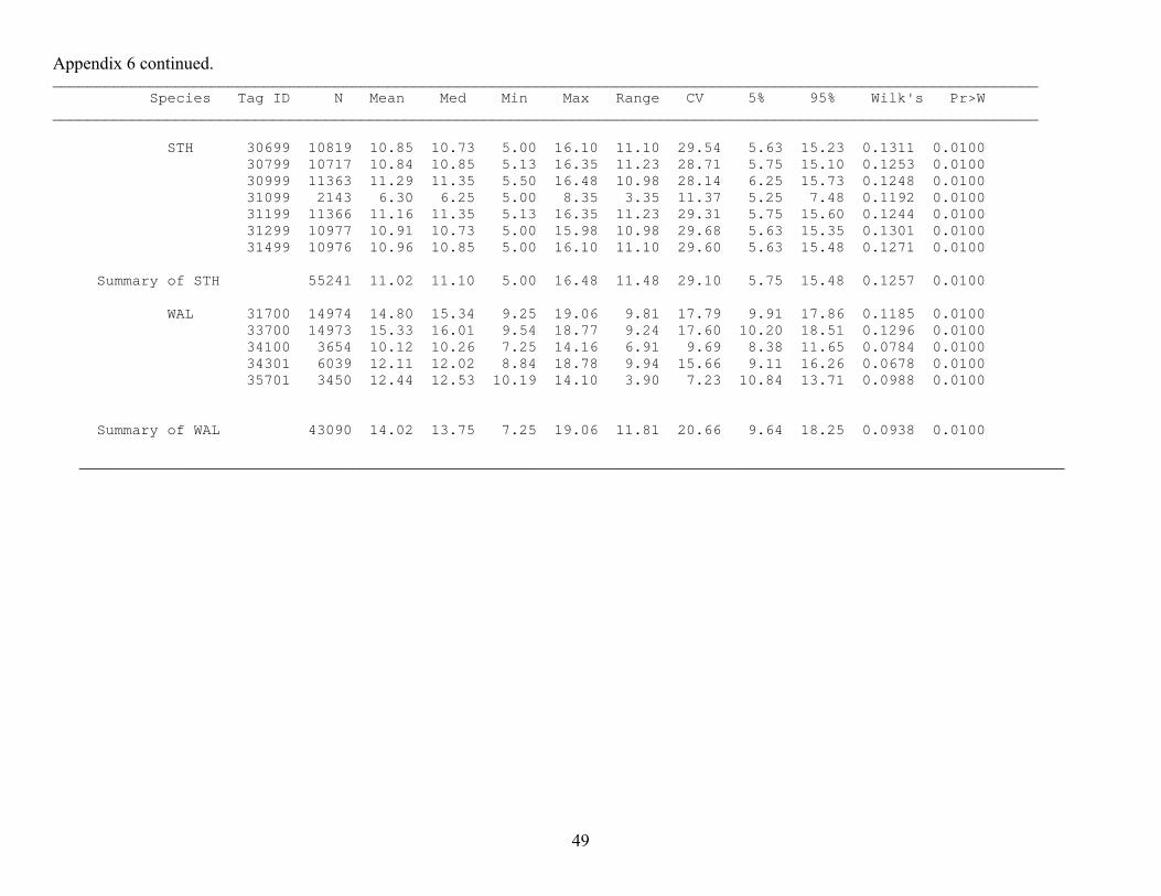
Appendix 6 continued. ________________________________________________________________________________________________________________ Species Tag ID N Mean Med Min Max Range CV 5% 95% Wilk's Pr>W ________________________________________________________________________________________________________________ STH 30699 10819 10.85 10.73 5.00 16.10 11.10 29.54 5.63 15.23 0.1311 0.0100 30799 10717 10.84 10.85 5.13 16.35 11.23 28.71 5.75 15.10 0.1253 0.0100 30999 11363 11.29 11.35 5.50 16.48 10.98 28.14 6.25 15.73 0.1248 0.0100 31099 2143 6.30 6.25 5.00 8.35 3.35 11.37 5.25 7.48 0.1192 0.0100 31199 11366 11.16 11.35 5.13 16.35 11.23 29.31 5.75 15.60 0.1244 0.0100 31299 10977 10.91 10.73 5.00 15.98 10.98 29.68 5.63 15.35 0.1301 0.0100 31499 10976 10.96 10.85 5.00 16.10 11.10 29.60 5.63 15.48 0.1271 0.0100 Summary of STH 55241 11.02 11.10 5.00 16.48 11.48 29.10 5.75 15.48 0.1257 0.0100 WAL 31700 14974 14.80 15.34 9.25 19.06 9.81 17.79 9.91 17.86 0.1185 0.0100 33700 14973 15.33 16.01 9.54 18.77 9.24 17.60 10.20 18.51 0.1296 0.0100 34100 3654 10.12 10.26 7.25 14.16 6.91 9.69 8.38 11.65 0.0784 0.0100 34301 6039 12.11 12.02 8.84 18.78 9.94 15.66 9.11 16.26 0.0678 0.0100 35701 3450 12.44 12.53 10.19 14.10 3.90 7.23 10.84 13.71 0.0988 0.0100 Summary of WAL 43090 14.02 13.75 7.25 19.06 11.81 20.66 9.64 18.25 0.0938 0.0100 ________________________________________________________________________________________________________________
49

50
Chapter II: The progression and lethality of gas bubble disease in
resident fish of Rufus Woods Lake. S. P. VanderKooi, R. G. Morris, J. W. Beeman, and A. G. Maule Abstract
Laboratory evaluations of gas bubble disease sign progression and time-to-death were conducted
at the Columbia River Research Laboratory for fish species resident to Rufus Woods Lake from
the summer of 2000 to spring of 2002. Species evaluated included: largescale sucker (LSS),
longnose sucker (LSS), northern pikeminnow (NPM), redside shiner (RSS), and walleye (WAL).
Total dissolved gas supersaturation (TDGS) levels evaluated were 115, 125 and 130%. Little
mortality was observed at 115% TDGS, yet the most dramatic signs were observed in every
species after prolonged exposure at this level of TDGS. Progression of GBD signs proved to be
unpredictable at any treatment level, with the exception that long-term exposure to 115%
resulted in the most exaggerated signs. Fish exposed to 125 and 130% TDGS died without
extensive sign formation, suggesting that prevalence and severity of signs are not predictive of
mortality. The time to 50% mortality (LT50) for all test species were nearly halved or better at
130% as compared to 125% TDGS. Species sensitivities for 125% TDGS were NPM ≥ LSS >
LNS > RSS > WAL and at 130% were LSS > NPM > LNS ≥ RSS > WAL. Largescale suckers
were the most sensitive of the two sucker species to TDGS.
51
Introduction
Gas-supersaturated water causes a condition known as gas bubble disease (GBD) in aquatic
organisms, and induces a variety of sub-lethal and lethal effects in fish and other aquatic species
(Weitkamp and Katz 1980). Historic total dissolved gas saturation in the tailrace below Grand
Coulee Dam has exceeded 140% (COE 2000) and fish kills attributed to gas-supersaturated
water below Grand Coulee Dam have occurred (Elston 1998). Similar total dissolved gas levels
have been found at other dams within the region (COE 2000), and this has resulted in extensive
research on the effects of GBD on salmonids in the Columbia River Basin (Ebel et al. 1975,
Stroud et al. 1975, Hans et al. 1999, Weiland et al. 1999, Mesa et al. 2000). While much of the
research has been focused on GBD impacts on salmon, predators of juvenile salmon or game fish
(Montgomery and Becker 1980, Bentley and Dawley 1981, Counihan et al. 1998), impacts of
GBD on resident fish have received less attention (Ryan et al. 2000).
Susceptibility to GBD varies between species (Stroud et al. 1975, Fickeisen and Montgomery
1978) and life history stage within a species (Weitkamp and Katz 1980, Alderdice and Jensen
1985, McDonough and Hemmingsen 1985, Jensen 1988, Krise and Herman 1991). Variations in
behavior or habitat preferences may also result in different susceptibilities to GBD. Each meter
of water depth compensates, via hydrostatic pressure, for approximately 10 % TDGS (Weitkamp
and Katz 1980). Juvenile Chinook salmon (Oncorhynchus tshawytscha) and steelhead (O.
mykiss) have been found to migrate at median depths of 1.7 – 2.7 m (Beeman et al. 1999). Fish
migrating at these depths would be able to compensate for TDGS levels from 117 – 126 %. Fish
occupying shallow habitats or near surface areas under similar TDGS conditions would be more
susceptible to GBD given the lack of hydrostatic compensation afforded them.
The impact a TDGS event has on a fish community depends on many factors including the level
of TDGS, the duration of the event, the suceptibility of each species, as well as the life-history
stages of each species present. Though the susceptibiltiy of juvenile salmonids has been
thoroughly studied (Dawley and Ebel. 1975, Stroud et al. 1975, Hans et al. 1999, Weiland et al.
1999, Mesa et al. 2000), little information exists on the susceptibility of resident species in the
Columbia River.

As part of a study to monitor the effects of TDGS on resident fish below Grand Coulee Dam, a
series of laboratory experiments were conducted on several resident species at the Columbia
River Research Laboratory (CRRL) in Cook, WA. Study objectives were to determine the
effects of several levels of TDGS on GBD in terms of progression of signs and time to mortality
of selected species of fish present in Rufus Woods Lake, which is the impounded Columbia
River between Chief Joseph Dam and Grand Coulee Dam (Figure 1).
Figure 1. Rufus Woods Lake
Methods
Test fish.--Trials were conducted from the summer of 2000 to spring of 2002, and study fish
included largescale sucker (LSS) Catostomus macrocheilus (mean weight (WT) ± SE = 30.0 ±
1.1 g, mean fork length (FL) ± SE = 136.7 ± 1.6 mm), longnose sucker (LNS) C. catostomus
(WT = 71.1 ± 2.5 g, FL = 180.8 ± 1.8 mm), northern pikeminnow (NPM) Ptychocheilus
oregonensis (WT = 34.6 ± 2.3 g, FL = 137.1 ± 2.7 mm), redside shiner (RSS) Richardsonius
balteatus (WT = 8.2 ± 0.3 g, FL = 87.7 ± 0.5 mm) and walleye (WAL) Stizostedian vitreum (WT
= 30.7 ± 1.5 g, FL = 153.1 ± 1.5 mm). Longnose sucker and redside shiner were collected from
Rufus Woods Lake and northern pikeminnow and largescale sucker were collected from the free-
flowing Hanford Reach of the Columbia River. Fish were collected by boat electrofisher (Smith-
Root 18-E Electrofishing Workboat, Model GPP Electrofisher, Vancouver, WA) using 400-500
V pulsed DC at 30 pulses/sec and 3-4 Amps. Fish were netted and placed in the electrofishing
boat's live well then transferred by dipnet to either a small concrete raceway supplied with well 52

53
water or 133 L mesh-walled containers anchored in the river and held for up to 2 days. Fish held
in the raceway were transferred by dipnet directly to a transport tank while fish held in-river
were transferred to the boat's live well, moved by boat to a transport vehicle, and transferred to a
transport tank. Fish were transported to CRRL in oxygenated well or river water. Walleye were
obtained from McKenzie Fish Company, Stacy, MN and shipped in chilled, oxygenated, salted
well water by truck to CRRL.
At CRRL, fish were acclimatized to well water heated to 12° C for a minimum of one week prior
to use. Excess dissolved gas was removed by passing the heated water through a packed
column; the TDGS in the holding tanks and control tanks for each experiment was maintained at
104.5 ± 0.2%. Walleye were salted initially to prevent disease and abrupt changes in water
quality. Fish were kept in outdoor 1,400-L flow-through circular fiberglass holding tanks and
were fed Deep-frozen Blood Worms™ (redside shiner) or Rangen Quality Feed for
Aquaculture™ (walleye, sucker species and northern pikeminnow) daily. Fish were not fed for
the duration of each test and were maintained under a natural photoperiod throughout the studies.
Experimental system. — Water supersaturated with atmospheric air was generated by water
heating and injecting air into water under pressure as described by Mesa et al. (2000) with the
exception that larger test tanks were used. The mean water volume (± SE) for the study tanks
was 154.8 ± 2.5 L and the mean water depth (± SE) was 26.0 ± 0.1 cm to minimize depth
compensation. Mean flow rate (± SE) was 4.8 ± 0.1 L/min. Water temperature, barometric
pressure, barometric pressure minus total pressure (delta P), and percent saturation was measured
throughout all studies using a Total Dissolved Gas and Oxygen Monitor, Model TBO-L
(Common Sensing, Inc. Clark Fork, ID). Nominal TDGS concentrations were also measured in
all tanks before and after each trial using the Common Sensing TDGS meter, a Weiss ES-2
saturometer (Eco Enterprises, Seattle, WA) or Tensionometer 300E (Alpha Designs, Victoria,
B.C.). Different meters were used due to meter malfunctions. All meters were calibrated
according to the manufacturer’s specifications.
Experimental procedure. —The progression of signs of GBD was evaluated in longnose sucker,
redside shiner and walleye at TDGS levels of 115, 125 and 130% and in largescale sucker and
northern pikeminnow at TDGS levels of 115 and 125% (Table 2). In separate experiments, the
time to 50% mortality (LT50) was determined in largescale sucker, longnose sucker, walleye,
redside shiner, and northern pikeminnow at TDGS levels of 125 and 130%. The LT50s for fish

54
at 115% TDGS were not determined as there was very little mortality for up to 4 weeks during
the progression of signs experiments. For progression of signs studies, varying numbers of fish
were stocked in each of four treatment and two control tanks (Table 2) which changed depending
upon availability of a species. For LT50 determinations, 10 fish were stocked in each of one
control and four treatment tanks, with the exception that only five fish were placed in a control
tank at 125 and 130% TDGS in northern pikeminnow tests due to limited supplies of this species
(Table 2).
In progression of signs studies, fish sampling was initiated at first mortality and three fish were
sampled at 2-h intervals from randomly designated pairs of treatment tanks with one fish being
removed from one tank and two from the other, alternately. In trials at 115% TDGS this process
was modified to sampling every 24 h due to little or no mortality. Fish were observed every 2 h
and sampled every 8 h after the first mortality at 115% TDGS. For LT50 determinations, dead
fish were removed at designated observation periods and evaluated for signs of GBD.
Sampling and examination. — Fish were rapidly netted and placed in a lethal dose of tricaine
methanesulfonate (MS-222; 200 mg/L, buffered 1:1 with sodium bicarbonate) made from the
supersaturated water supplying the treatment tanks. Mortalities were also removed at the
sampling or observation time and placed in supersaturated water until evaluation. Control fish
were sampled at the end of each trial and were placed in buffered MS-222 prepared with water
from the control tanks. The fork length and weight of each fish was measured and the fish was
placed left–side up on a paper towel moistened with water from the appropriate test solution.
Visual examinations of GBD signs were then conducted for all sampled fish using the method
described by Mesa et al. (2000). This included evaluation of the lateral line, unpaired fins
(dorsal, caudal and anal fins), and the left eye. Fish were examined externally using a dissecting
microscope with 8 – 40X zoom magnification. A ruler-like micrometer divided into units of 0.5
mm was used to measure the percent of the lateral line occluded with bubbles. The left eye and
unpaired fins were examined and assigned a rank based on the percent of area covered with
bubbles: 0 = no bubbles; 1 = 1 - 25% covered; 2 = 26 - 50% covered; 3 = 51 - 75% covered; 4 >
75% covered. The first gill arch was then excised with surgical scissors and placed in a drop of
the supersaturated water on a microscope slide. Gill filaments were then severed from the arch
with a razor blade and immediately analyzed using a compound microscope under 40 – 100X
magnification. The total number of filaments examined and the number of filaments with at least
one intravascular bubble were recorded.

55
Data analysis. —The mean percent occlusion of the lateral line, mean percent of gill filaments
with gas bubbles in the vasculature, and the mean severity rating from the unpaired fins was
calculated for each progression of signs trial using only fish sampled live. The responses of
individuals were also plotted in each of these categories versus exposure time by species for each
TDGS level tested. Data from individuals were examined visually and if necessary, transformed
to normalize distribution and equalize spread. Appropriate transformations were determined by
examination of residual plots as suggested by Ramsey and Schafer (1997).
The relationship between severity of GBD signs and exposure time to each TDGS level was
described using linear regression. The slopes of the regression lines were considered to differ
significantly from zero at a level of α = 0.05. Comparisons of means were accomplished using
General Linear Models (GLM, SAS 1999) and the Ryan’s (Ryan-Einot-Gabriel-Welsch)
multiple range test (α = 0.05) as described by Toothaker (1993). Parametric comparisons of all
fish used in a given experiment were considered valid for these data because time of exposure
was not found to be a significant factor in the development of most of the signs as indicated by
regression analysis. Signs of GBD from mortalities in progression studies were not included in
data analysis. For each mortality trial, cumulative mortality as a percentage over time was
plotted. The LT50 was estimated by extrapolation from a curve fitted to the mortality data with
simple straight-line connections through each point.
Results
Water Quality
Trials were conducted from May 2000 to April 2002 and well water with the following water
quality characteristics was used for all testing: hardness (as CaCO3) <10 mg/L; alkalinity (as
CaCO3), 20 mg/L; pH, 6.6. National Testing Laboratories LTD conducted chemical analysis of
the well water for water quality analysis and potential contaminants. No contaminants were
found above minimum detection limits. Water temperature was maintained at about 12.0 ºC for
all studies (Table 1). Total dissolved gas supersaturation varied little from the desired levels
throughout the trials (Table 1), and control tank TDGS (± SE) was consistent for all studies at
104.3 ± 0.13%; N = 50.

56
Largescale sucker
Progression of GBD signs trials for LLS were conducted at 115 and 125% TDGS. Percent
lateral line occlusion and percent of gill filaments with bubbles were significantly higher in fish
exposed to 125% TDGS than to 115% (Table 2). Fin severity ratings, on the other hand, did not
differ significantly between the two TDGS levels. Eye bubble severity rating did not differ
significantly between treatment levels and over 90% of the values at any treatment were zero.
Exophthalmia (popeye) was only observed in LSS at 115% TDGS after 216 hours of exposure.
Low-level mortality (9%) occurred in LSS over the 17 d of the progression of GBD signs trial at
115% TDGS. The slopes of the regression lines describing lateral line occlusion and gill
filament bubbles developing over time did not differ from zero (Figures 1A and B). The slope of
the regression line for fin-severity ratings differed significantly from zero (Figure 1C), but the
regression had little explanatory power (i.e., r2 = 0.13) due to high levels of inter-individual
variation. Mortality levels were high (72%) during the 20-h progression of GBD signs trial at
125% TDGS. None of the regression lines describing sign development over exposure time in
the 125% TDGS trial had slopes that differed from zero (Figure 2). Evaluation of control fish at
the termination of each study revealed no signs of gas bubble disease. Mortality rates (as LT50)
were 17 h at 125% TDGS and 9.5 h at 130% (Table 3).
Longnose sucker
Progression of GBD signs trials for LNS were conducted at 115, 125, and 130% TDGS. Lateral
line occlusion and percent of gill filaments with bubbles followed the same pattern observed in
LSS—lateral line occlusion was lowest at 115% TDGS (Table 2) and increased to its highest
levels at 125% and 130%. Although lateral line occlusion declined slightly between 125 and
130% TDGS, the values did not differ significantly. Over 80% of the fin ratings were between
zero and one for all treatments and there was no statistically significant difference between fin
ratings for any treatment.
There were no eye bubbles in over 94% of the LNS examined, and there was no difference
between treatment levels. Exophthalmia was observed in this species only at 115% TDGS after
168 h of exposure. Mortality levels were low (8%) during the 27-d progression of GBD signs
trial at 115% TDGS. The slopes of the regression lines for lateral line occlusion (square root
transformed), gill filaments with bubbles (loge transformed), and fin-severity ratings over time

57
all differed significantly from zero (P = 0.023; Figure 3). Explanatory power of all three
regressions was low (r2 ≤ 0.15). In the progression of GBD signs trial at 125% TDGS, mortality
reached 44% in 71 h. None of the slopes of regression lines describing the GBD sign
development over exposure time differed from zero (Figure 4). High levels of mortality (62%)
were observed during the 50-h GBD progression of signs trial at 130% TDGS. The slopes of the
regression lines describing lateral line occlusion and gill filament bubble development over time
differed significantly from zero (P < 0.02), but high variability between individuals resulted in
relatively weak explanatory values for these regressions (Figures 5). The slope of the regression
line for fin-severity ratings to exposure time did not differ from zero (Figure 5C).
Evaluation of control fish at the termination of each study revealed no signs of gas bubble
disease during any study and control survival was 100% for all studies except the 115%
progression of signs evaluation. One third of the control fish and one tenth of treated fish died
during this trial. This loss appeared to be related to holding stress and all mortalities were
evaluated but not used in GBD evaluation statistics. No GBD signs were observed in control
mortalities. The LT50s were 56 h at 125% TDGS and 30 h at 130% (Table 3).
Northern pikeminnow
Progression of GBD in NPM was monitored in trials at 115 and 125% TDGS. Gas bubble
disease signs followed the same pattern as those observed in largescale sucker between 115 and
125% TDGS. Lateral line occlusion did not differ significantly between treatment levels and
percent of gill filaments with bubbles increased significantly between treatment levels (Table 4),
while fin severity ratings were significantly lower at 125% than 115%. Over 80% of fin ratings
at any treatment level were either zero or one.
The progression of GBD signs trial at 115% TDGS lasted for 26 d, and there was one mortality.
Mortality levels reached 70% during the 20 h of the progression of GBD signs trial at 125%
TDGS. None of the regression lines describing the development of lateral line occlusion,
prevalence of gill filaments with bubbles, or fin-severity ratings over time in either the 115% or
the 125% trial had slopes that differed from zero (Figures 6 and 7). The percent of bubles in the
gill filaments was significantly higher at 125% than 115% TDGS (Table 2). There were no
bubbles in the eyes of any fish in these experiments and exophthalmia was observed in this
species only at 115% TDGS after 168 h of exposure. Control fish revealed no signs of gas

58
bubble disease for any study nor were there any control mortalities. Due to insufficient supplies
of fish, the progression of signs in NPM at the highest TDGS level was not examined. The LT50
was 15.3 h at 125% TDGS and 10 h at 130% (Table 3).
Redside shiner
Progression of GBD in RSS was monitored in trials at 115, 125, and 130% TDGS. Mean levels
of lateral line occlusion, gill filaments with bubbles, and fin severity ratings all increased
significantly between 115 and 130% TDGS (Table 2). However, over 90% of the fin ratings
were either zero or one for all treatment levels. Redside shiner was the only species to exhibit
significant eye bubble development between TDGS levels (Table 2); however, over 74% of the
data collected were still zero. Redside shiner also exhibited a trend in exophthalmia opposite to
the other species showing no exophthalmia at 115% and elevated levels at 125 and 130% TDGS.
There were no mortalities over the 30-d of the progression of GBD signs trial at 115% TDGS.
Mortality levels were 19% and 37% for the 125% and 130% TDGS progression of GBD signs
trials%, respectively. None of the slopes for regression lines describing lateral line occlusion,
gill filament occlusion with bubbles, or fin bubble development over exposure time in any of the
trials with redside shiner differed significantly from zero (Figs 8, 9, and 10). Evaluation of
control fish revealed no signs of gas bubble disease for any study and there were no control
mortalities in any redside shiner study. The LT50s for RSS were 116 h at 125% TDGS and 31 h
at 130% (Table 3).
Walleye
Progression of GBD in WAL was monitored in trials at 115, 125, and 130% TDGS. The percent
of gill filaments with bubbles, eye, caudal and anal fin severity ratings did not differ significantly
at any TDGS (Table 2) while mean dorsal fin rating differed significantly only between 125 and
130% TDGS (P < 0.01). Over 75% of the fin severity ratings were zero. Mean percent lateral
line occlusion differed significantly between treatments (125 %> 130 %> 115%, P < 0.0001).
The regression lines describing the progression of lateral line occlusion over time revealed
different trends at each TDGS. At 115% TDGS, the slope of the regression line was
significantly different from zero (P < 0.0001) and lateral line occlusion declined over time
(Figure 11). At 125% TDGS, the slope of the regression line did not differ significantly from

59
zero (Figure 12; P = 0.25) while at 130% TDGS, the slope of the lateral line occlusion regression
line differed significantly from zero (P < 0.0001) and lateral line occlusion increased over time
(Figure 13). Mean fin severity ratings differed significantly from zero at 115% and 130% but
not at 125% TDGS (Figures 11, 12, and13). Regressions for eye bubble severity did not differ
significantly from zero at any TDGS and over 97% of our values were zero (Figures 13, 12, and
13). Exopthalmia was first noted at 168 h. in the 115% progression of signs study and was fairly
common towards the end of the study. Popeye was not observed in either the 125% or 130%
TDGS progression of signs study. Evaluation of control fish revealed no signs of gas bubble
disease for any study and there were no control mortalities in any walleye study. The LT50 was
169 h at 125% TDGS and 62 h at 130% (Table 3).
Interspecies Comparisons
115% TDGS — Northern pikeminnow and walleye had significantly higher lateral line occlusion
(24.7% and 21.9%, respectively) than any of the other species tested (Table 4). No significant
difference in percent of gill filament with bubbles or eye bubble formation was found in any
species (Table 4) at 115% TDGS. Largescale sucker exhibited significantly greater fin bubble
formation than longnose sucker, northern pikeminnow and walleye, which did not differ, while
redside shiner ranked significantly lower than all other test species.
No LT50s were determined for any species at this exposure level due to the extremely low levels
of mortality. Largescale sucker exhibited a 10% mortality rate in the progression of signs study.
Longnose sucker also exhibited a 10% mortality rate at this treatment but the control mortality
(33%) precludes any discussion of this mortality in relation to GBD.
125% TDGS — Walleye exhibited the highest levels of lateral line occlusion (Table 4), followed
by northern pikeminnow. Redside shiner, largescale sucker and longnose sucker had the lowest
and were not significantly different from each other. Multiple comparison tests for bubbles in
gill filaments indicated that the two sucker species did not differ but were significantly higher
than walleye, northern pikeminnow or redside shiner (Table 4). Redside shiner, walleye and
northern pikeminnow did not differ, but largescale sucker fin bubble development was
significantly higher than the four other species, which were effectively equal. It is worth noting ,
however, that none of the mean fin ratings exceeded 1.0. There was no significant difference in

60
eye bubble formation between any species at this treatment (Table 4), however, 94.4% of our eye
bubble data was zero.
Walleye had the longest LT50 at 125% TDGS, exceeding 160 hours (Figure 14). Redside shiner
were the next most resistant with an LT50 of 113 hours. Largescale sucker and northern
pikeminnow were the most sensitive species at this level with LT50s at approximately 16.5 and
15.5 hours, respectively. Largescale sucker and northern pikeminnow also exhibited similar
mortality curves (Figure 15).
130% TDGS. — Only three species, longnose sucker, walleye, and redside shiner were tested for
progression of signs at this level due to inadequate supplies of fish. Walleye exhibited
significantly higher lateral line occlusion than redside shiner, which was significantly higher than
longnose sucker (Table 4). Walleye exhibited significantly lower percent bubbles in gill
filaments than redside shiner or longnose sucker, which did not differ from each other (Table 4).
Longnose sucker fin bubble rank was significantly higher than redside shiner, while walleye
ranked intermediate and did not differ from either species. None of these mean fin rankings
exceeded 1.0. There was a significant difference in eye bubble prevalence between redside
shiner and longnose sucker (Table 4) although over 86% of our observations were zero for all
three species.
The LT50s for all species were nearly halved or better at 130% as compared to 125% TDGS
(Table 3) with the exception of the most sensitive species, northern pikeminnow, which
exhibited a 31% decrease. Walleye were the most resistant species with an LT50 of 62 hours.
Redside shiner and longnose sucker exhibited almost identical LT50s at 130% TDGS of
approximately 31 hours. Largescale sucker and northern pikeminnow also exhibited extremely
close LT50s of 9.5 and 10.5 hours, respectively (Table 3). The mortality curve and the LT50 for
walleye at 130% TDGS were very similar to those of longnose sucker at 125% TDGS (Figure 7).
Discussion
Perhaps the most interesting finding in our study is the species-specific variability in the rates of
mortality as measured by LT50 (Table 3 and Figures 14 and 15). There were 10-fold differences
in the LT50s of fish exposed to 125% TDGS and 6-fold differences when fish were exposed to
130% TDGS. It is possible, and perhaps likely, that these differences in sensitivity to high

61
TDGS will differentially impact fish populations in Rufus Woods Lake. For example, a 24-h
spike in TDGS to 130% would kill a greater proportion of largescale suckers and northern
pikeminnows as compared to walleye and redside shiners—assuming that the populations are at
similar depths. Similarly, the difference in sensitivity might shift survival or fitness advantage to
the most resistant species. For example, at low TDGS or short exposure times, the ability of
sensitive fish (e.g., largescale suckers) to avoid predation might be reduced, while piscivorous
walleye would be relatively free from adverse effects and could actively prey upon the suckers.
In our examination of five fish species resident to Rufus Woods Lake we found no predictive
relation between the progression of signs of GBD and mortality caused by a combination of level
of TDGS and time of exposure. Our results also suggest that the progression of GBD in terms of
severity of signs is species dependent. That is, for some species and TDGS level there was a
significant increase in severity of signs in one or more location on the fish (e.g., gills, lateral line,
or skin) with increasing time of exposure. There were significant positive relations between some
signs and time of exposure at 115% TDGS in walleye, both sucker species tested, and at 130%
TDGS for longnose sucker. This was not, however, true of northern pikeminnow or redside
shiner, in which signs did not change through time in any exposure trials. These findings are
consistent with those of Ryan et al. (2000) who reported that severity of GBD signs was a weak
predictor, compared to prevalence of signs, for modeling susceptibility to TDGS in non-salmonid
fish from the Snake and lower Columbia rivers. On the other hand, Mesa et al. (2000) observed
that GBD signs increased significantly through time for virtually all tests with juvenile Chinook
salmon Oncorhyncus tshawytscha and steelhead O. mykiss at 110%, 120% and 130% TDGS.
The species used in this study may account for the lack of significant relations between signs of
GBD and length of exposure to TDGS, as the signs selected for evaluating the progression of
GBD may not be appropriate for all species. The monitoring design for these trials was based on
that used by Mesa et al. (2000) to describe GBD severity trends over time in juvenile Chinook
salmon and steelhead in laboratory studies. They found stronger correlations between severity
and time at higher TDGS levels. Ryan et al. (2000), however, found that severity of GBD
symptoms supplied weak or variable relations with TDGS exposure in in-situ studies and thus
were prevented from making a predictive model describing GBD signs in non-salmonid fishes.
Our results concur with those of Ryan et al. (2000) and indicate that relations between GBD sign
severity and their progression over time are highly variable between individuals and species.

62
While GBD signs generally did not worsen over time, the severity of signs increased somewhat
as TDGS level increased. In addition, the LT50 decreased for all species as TDGS level
increased (Table 3). The inverse relation between mean severity of signs and time to death
suggests that at the higher TDGS, fish are dying prior to formation of GBD signs. Stroud et al.
(1975) observed that fish exposed to high TDGS died before external lesions occurred. Colt et
al. (1985) also found that GBD signs in mortality studies with channel catfish declined over time.
Dawley and Ebel (1975) noted that severity of signs decreased in juvenile Chinook salmon as
TDGS increased and concluded that the fish died from cardiac or branchial artery occlusion
before the signs could develop.
The magnitude of responses for each GBD sign varied by species and TDGS exposure level.
The two sucker species usually exhibited signs closer to each other than to the other species
(Table 4), yet had very different LT50s (Table 3). Lateral line occlusion may be an appropriate
indicator of GBD severity within a species, however, the same comparisons between species
may be inappropriate. Northern pikeminnow and walleye exhibited 25% and 22% lateral line
occlusion, respectively, at 115% TDGS, while all other species had occlusion levels below 2%
(Table 4). Lateral line occlusion was greater in all species at 125% than at 115% TDGS, and
species specificity changed dramatically, with the greatest mean lateral line occlusion occurring
in walleye (72%), the next being pikeminnow (28%) and much lower levels in the other species
(Table 4). Lateral line occlusion did not change in longnose sucker, but increased significantly
in redside shiner between 125% and 130% (Table 4). Longnose sucker exhibited the lowest
lateral line occlusion at every TDGS level. Walleye exhibited the largest change in lateral line
occlusion between treatment levels (Table 2).
A possible explanation for the observed differences in lateral line occlusion may be differences
in lateral line pore size between species. During experiments with longnose sucker, the
relatively large size of their lateral line pores was noted. Bubbles occluding the lateral line were
also observed escaping via these pores and lines of bubbles were frequently observed in the
suckers’ mucous coat immediately above the lateral line pores (Morris et al. 2003; Chapter V,
this report). Subsequent measurements of lateral line pore diameter revealed pores were largest
in longnose sucker, slightly smaller in largescale sucker, smallest in northern pikeminnow,
walleye and redside shiner (Morris et al. 2003; Chapter V, this report). These pore sizes were
inversely related to levels of lateral line occlusion, suggesting that fish with larger pores are less
likely to develop high levels of lateral line occlusion.

63
Observations of bubbles exiting the lateral line via large pores also suggests a mechanism by
which some fish may be able to dissipate excess dissolved gas from the circulation, thus
involving the lateral line in cutaneous respiration. Since suffocation resulting from haemostasis
is one cause of death from GBD in acute exposures, it is reasonable to assume that fish with
differing rates of cutaneous respiration, as described in salmonids by Rombough and Ure (1991),
will exhibit different levels of resistance to GBD. Differing cutaneous respiration rates may also
be a stochastic factor in the formation of GBD signs. Results from our mortality trials, however,
indicate that if this mechanism does exist it has little influence on mortality from GBD and the
relative cutaneous respiration efficiencies for the species we tested are not known. The shortest
LT50s at both 125% and 130% TDGS were observed in northern pikeminnow and largescale
sucker, fish with the second highest and next to lowest levels of lateral line occlusion,
respectively (Table 4).
Changes in the percent of gill filaments with bubbles as TDGS increased followed a pattern
similar to that observed in lateral line occlusion, but the responses of individual species were
quite different. At 115% TDGS, species differences in percent of gill filament with bubbles
were apparent with largescale sucker having small but significantly higher levels of affected gills
than northern pikeminnow and redside shiner (Table 3). The percentage of gill filaments with
bubbles was low for all species at 115% TDGS and increased in each at 125%, most notably in
longnose sucker and largescale sucker. The two sucker species exhibited significantly higher gill
filament occlusion than walleye, northern pikeminnow or redside shiner at 125% TDGS (Table
3). As with lateral line occlusion, we found that the percent of gill filaments with bubbles was
greater in redside shiner at 130% than at 125% TDGS but decreased significantly in longnose
sucker between 125 and 130% TDGS (Table 3). Walleye revealed the least amount of gill
filaments with bubbles at 125% and 130% TDGS of any of the species tested, which may be one
reason for their insensitivity to elevated TDGS. However, northern pikeminnow, the most
sensitive species at 125% TDGS, had relatively low levels of gill filaments with bubbles at 125%
TDGS while largescale sucker, the next most sensitive species at 125% TDGS had the next
highest levels of affect gill filaments.
Bubble formation in the gill filaments and cardiac occlusion during TDGS exposure are thought
to be the immediate cause of death in fish (Marsh and Gorham 1905, Dawley and Ebel 1975,
Weitkamp and Katz 1980). The LT50 in longnose sucker at 130% TDGS was just over half that

64
of the trial at 125% although percent of gill filaments with bubbles declined between 125 and
130% TDGS. Similar to the conclusions of Mesa et al. (2000) working with Chinook salmon,
these results suggest that while bubbles in the gill filaments of resident fish may be related to
mortality, they cannot be used to predict mortality risk to individuals. The inability to predict
risk may be due to the rapidity with which lethal bubbles form. Individual variability in gill
filament blood vessel morphology and blood flow rates may influence when and where gas
bubbles form, and how large they become.
The results from evaluating the severity of gas bubble formation in fins were quite different than
the other signs monitored. In comparing trials at 115 and 125% TDGS, fin ratings decreased
slightly in largescale sucker and decreased significantly in northern pikeminnow, remained
unchanged in longnose sucker, and increased significantly in redside shiner (Table 3). Fin
severity ratings were significantly higher at 130% TDGS in redside shiner and slightly higher in
longnose sucker. One difficulty with the fin rating data is that over 60% of our fin ratings were
either zero or one. The results from measuring fin severity highlights the unique responses each
species has to TDGS exposure. It is interesting to note that the two species in which mean fin
severity declined were the most susceptible, in terms of mortality rates, to TDGS. These results
concur with Stroud et al. (1975) and Dawley and Ebel’s (1975) assertions that the fish die prior
to the formation of signs at higher TDGS levels. Activity is thought to be one factor in GBD
sign development (Montgomery and Becker 1980, McDonough and Hemmingsen 1985). Our
results, however, show the most active species in these studies—northern pikeminnow and
redside shiner—exhibited opposite trends in fin sign development. All of the species we tested
exhibited decreased activity between treated and control tanks and tended to settle on or swim
slowly near the bottom of the tanks. Decreased activity has been noted in numerous studies
(Dawley and Ebel 1975, Stroud et al. 1975, Nebeker et al. 1976, Weitkamp et al. 1980, Bentley
and Dawley 1981, Krise and Meade 1988, Krise 1993, Hans et al. 1999) and is usually attributed
to efforts by the fish to compensate for TDGS. Such lethargic behavior would tend to minimize
bubble formation due to movement and points to the possibility that TDGS may have an
anesthetic effect that might be related to nitrogen narcosis (A. V. Nebeker, personal
communication).
Evaluation of bubble formation on the eyes proved to be unproductive in estimating the impact
of TDGS in four out of the five species studied, and of little predictive value on redside shiner as
mean eye bubble severity rating did not exceed 0.3 for this species. While Krise and Smith
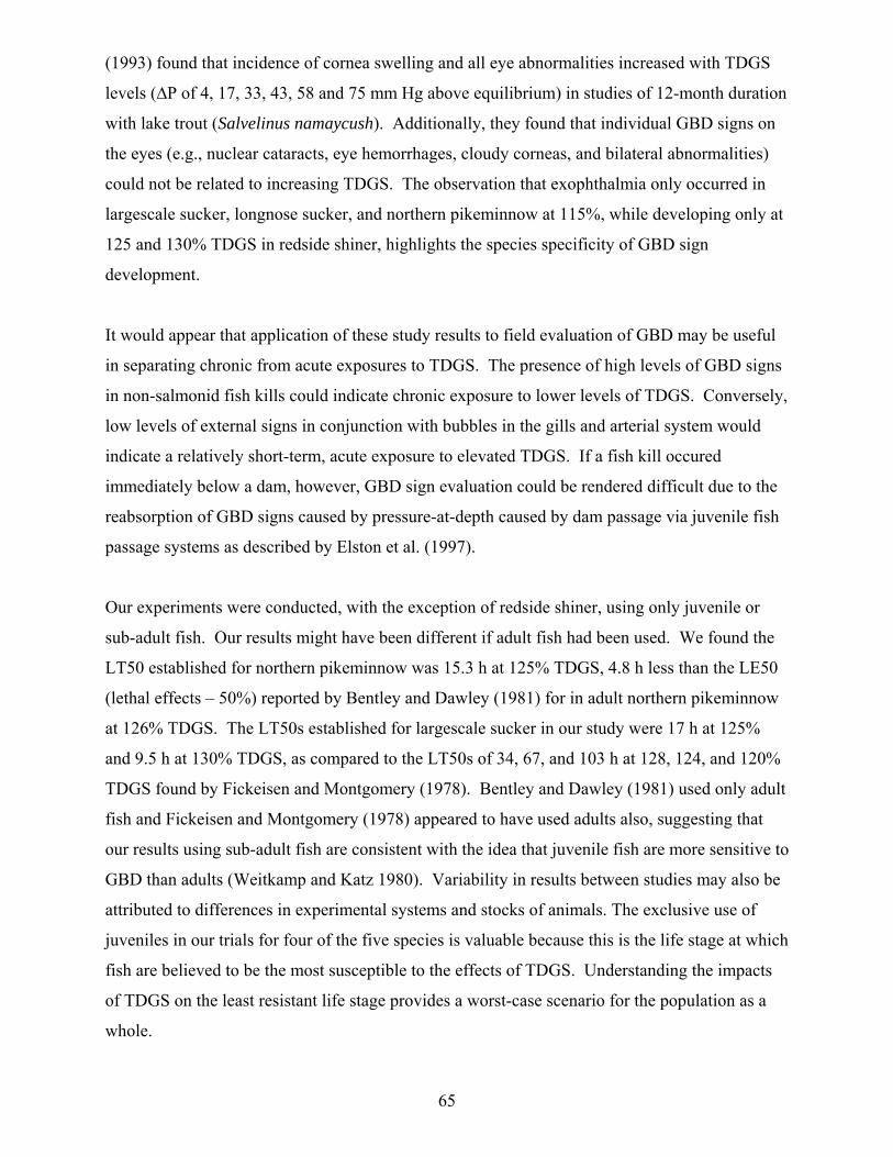
65
(1993) found that incidence of cornea swelling and all eye abnormalities increased with TDGS
levels (∆P of 4, 17, 33, 43, 58 and 75 mm Hg above equilibrium) in studies of 12-month duration
with lake trout (Salvelinus namaycush). Additionally, they found that individual GBD signs on
the eyes (e.g., nuclear cataracts, eye hemorrhages, cloudy corneas, and bilateral abnormalities)
could not be related to increasing TDGS. The observation that exophthalmia only occurred in
largescale sucker, longnose sucker, and northern pikeminnow at 115%, while developing only at
125 and 130% TDGS in redside shiner, highlights the species specificity of GBD sign
development.
It would appear that application of these study results to field evaluation of GBD may be useful
in separating chronic from acute exposures to TDGS. The presence of high levels of GBD signs
in non-salmonid fish kills could indicate chronic exposure to lower levels of TDGS. Conversely,
low levels of external signs in conjunction with bubbles in the gills and arterial system would
indicate a relatively short-term, acute exposure to elevated TDGS. If a fish kill occured
immediately below a dam, however, GBD sign evaluation could be rendered difficult due to the
reabsorption of GBD signs caused by pressure-at-depth caused by dam passage via juvenile fish
passage systems as described by Elston et al. (1997).
Our experiments were conducted, with the exception of redside shiner, using only juvenile or
sub-adult fish. Our results might have been different if adult fish had been used. We found the
LT50 established for northern pikeminnow was 15.3 h at 125% TDGS, 4.8 h less than the LE50
(lethal effects – 50%) reported by Bentley and Dawley (1981) for in adult northern pikeminnow
at 126% TDGS. The LT50s established for largescale sucker in our study were 17 h at 125%
and 9.5 h at 130% TDGS, as compared to the LT50s of 34, 67, and 103 h at 128, 124, and 120%
TDGS found by Fickeisen and Montgomery (1978). Bentley and Dawley (1981) used only adult
fish and Fickeisen and Montgomery (1978) appeared to have used adults also, suggesting that
our results using sub-adult fish are consistent with the idea that juvenile fish are more sensitive to
GBD than adults (Weitkamp and Katz 1980). Variability in results between studies may also be
attributed to differences in experimental systems and stocks of animals. The exclusive use of
juveniles in our trials for four of the five species is valuable because this is the life stage at which
fish are believed to be the most susceptible to the effects of TDGS. Understanding the impacts
of TDGS on the least resistant life stage provides a worst-case scenario for the population as a
whole.

66
The results of our study suggest that the severity of the GBD signs monitored are poor indicators
of the duration of TDGS exposure and inadequate as predictors of mortality in largescale sucker
and longnose sucker, northern pikeminnow, redside shiner, and walleye. Our results combined
with length-frequency distributions from the species composition in Rufus Woods Lake (Venditti
et al. 2001) suggest that juvenile largescale sucker and bridgelip sucker (C. columbianus) may be
more susceptible to GBD in the wild than are longnose sucker. The results of our laboratory
experiments will not allow us to predict mortality of resident fish in the field based solely on the
prevalence and severity of signs of GBD. However, these results can be combined with data on
TDGS and species-specific depth behavior (see Chapter II) to make an assessment of the relative
risk experienced by resident fish in Rufus Woods Lake during high TDGS events.

References Alderdice, D. F. and J. O. T. Jensen. 1985. An explanation for the high resistance of incubating
salmonid eggs to atmospheric gas supersaturation of water. Aquaculture 49:85-88 Beeman, J. W., T. C. Robinson, S. P. VanderKooi, and P. V. Haner. 1999. Gas Bubble Trauma
Monitoring and Research of Juvenile Salmonids, 1998 Annual Report. Prepared by U. S. Geological Survey for Bonneville Power Administration, Portland, OR, Contract 96-AI-93279.
Bentley, W.W., and E. M. Dawley. 1981. Effects of supersaturated dissolved atmospheric gases
on northern squawfish, Ptychocheilus oregonensis. Northwest Science 55:50-61. Colt, J., K. Orwicz, and D. Brooks. 1985. The effect of gas supersaturation on the growth of
juvenile channel catfish, Ictalurus punctatus. Aquaculture 50:153-160. Corps of Engineers. 2000. 1999 total dissolved gas monitoring- Columbia and Snake rivers.
US Army Corps of Engineers, Northwestern Division, NorthPacific Region, Water Management Devision, Reservoir Control Center, Water Quality Section, Portland, Oregon.
Counihan, T. D., A. I. Miller, M. G. Mesa, and M. J. Parsley. 1998. The effects of dissolved gas
supersaturation on white sturgeon larvae. Transactions of the American Fisheries Society 127:316-322.
Dawley, E.M., and W.J. Ebel. 1975. Effects of various concentrations of dissolved atmospheric
gas on juvenile Chinook salmon and steelhead trout. Fishery Bulletin 73(4): 787-796. Ebel, W.J, H.L. Raymond, G.E. Monan, W.E. Farr, and G.K. Tanonaka. 1975. Effect of
atmospheric gas supersaturation caused by dams on salmon and steelhead trout of the Snake and Columbia rivers. Northwest Fisheries Center Processed Report, Seattle, WA.
Elston, R. 1998. Fish kills in resident and captive fish caused by spill at Grand Coulee Dam in
1997: final report. Prepared by Aquatechnics Inc., Carlsborg, Washington for the Confederated Tribes of the Colville Reservation, Nespelem, Washington and Columbia River Fish Farms, Omak, Washington.
Elston, R., J. Colt, S. Abernathy, and W. Maslen. 1997. Gas bubble reabsorption in Chinook
salmon: pressurization effects. Journal of Aquatic Animal Health 9: 317-321. Feder, M. E., W. W. Burggren, and J. B. Graham. 1988. Introduction to the symposium:
Cutaneous exchange of gases and ions. American Zoologist 28:941-944. Fickeisen, D. H., and J. C. Montgomery. 1978. Tolerances of fishes to dissolved gas
supersaturation in deep tank bioassays. Transactions of the American Fisheries Society 107:376-381.
67

Hans, K. M., M. G. Mesa, and A. G. Maule. 1999. Rate of disappearance of gas bubble trauma signs in juvenile salmonids. Journal of Aquatic Animal Health 11:383-390.
Jensen, J.O.T. 1988. Combined effects of gas supersaturation and dissolved oxygen levels on
steelhead trout (Salmo gairdneri) eggs, larvae, and fry. Aquaculture 68:131-139. Krise, W. F., and J. W. Meade. 1988. Effects of low-level gas supersaturation on lake trout
(Salvelinus namaycush). Canadian Journal of Fisheries and Aquatic Science 45:666-674. Krise, W. F., and R. L. Herman. 1991. Resistance of underyearling and yearling atlantic salmon
and lake trout to supersaturation with air. Journal of Aquatic Animal Health 3:248-253. Krise, W. F. 1993. Effects of one-year exposures to gas supersaturation on lake trout. The
Progressive Fish-Culturist 55:169-176. Krise, W. F., and R. A. Smith. 1993. Eye abnormalities of lake trout exposed to gas
supersaturation. The Progressive Fish-Culturist 55:177-179. Marsh, M.C. and F.P. Gorham. 1905. The gas disease in fishes. Report of the United States
Bureau of Fisheries for 1904. McDonough, P.M., and E.A. Hemmingsen. 1985. Swimming movements initiate bubble
formation in fish decompressed from elevated gas pressures. Comparative Biochemistry and Physiology 81A(1):209-212.
Mesa, M. G., L. K. Weiland, and A. G. Maule. 2000. Progression and severity of gas bubble
trauma in juvenile salmonids. Transactions of the American Fisheries Society 129:174-185.
Montgomery, J. C., and C. D. Becker. 1980. Gas bubble disease in smallmouth bass and
northern squawfish from the Snake and Columbia rivers. Transactions of the American Fisheries Society 109:734-736.
Morris, R. G., J. W. Beeman, S. P. Vanderkooi, and A. G. Maule. 2003. Lateral line pore
diameters correlate with the development of gas bubble trauma signs in several Columbia River fishes. Comparative Biochemistry and Physiology Part A 135:309-320.
Nebeker, A. V., D. G. Stevens, and R. K. Stroud. 1976. Effects of air-supersaturated water on
adult sockeye salmon (Oncorhynchus nerka). Journal of the Fisheries Research Board of Canada 33:2629–2633.
Ramsey, F. L., and D. W. Schafer. 1997. The Statistical Sleuth: A Course in Methods of Data
Analysis. Duxbury Press, Belmont California.
68

Rombough, P. J. and D. Ure. 1991. Partitioning of oxygen uptake between cutaneous and branchial surfaces in larval and young juvenile Chinook salmon Oncorhynchus tshawytscha. Physiological Zoology 64(3):717-727.
Ryan, B. A., E. M. Dawley, and R. A. Nelson. 2000. Modeling the effects of supersaturated
dissolved gas on resident aquatic biota in the main-stem Snake and Columbia rivers. North American Journal of Fisheries Management 20:180-192.
SAS (Statistical Analysis System). 1999. SAS Proprietary Software Release 8.1. Copyright
1999-2000 by SAS Institute Inc., Cary, North Carolina, USA. Stroud, R. K., G. R. Bouck, and A. V. Nebeker. 1975. Pages 435-449 in Pathology of acute and
chronic exposure of salmonid fishes to supersaturated water in Chemistry and Physics of Aqueous Gas Solutions. The Electrochemical Society, Inc.
Toothaker, L.E. 1993. Multiple Comparison Procedures. Sage Publications, Inc. Newbury Park,
CA. 96 pp. Venditti, D. A., T. C. Robinson, J. W. Beeman, B. J. Adams, and A. G. Maule. 2001. Gas
bubble disease in resident fish below Grand Coulee Dam. 1999 Annual Report of Research. A report to the U. S. Geological Survey and the U. S. Bureau of Reclamation, 28 p.
Weiland, L. K., M. G. Mesa, and A. G. Maule. 1999. Influence of infection with Renibacterium
salmoninarum on susceptibility of juvenile spring Chinook salmon to gas bubble trauma. Journal of Aquatic Animal Health 11:123-129.
Weitkamp, D. E., and M. Katz. 1980. A review of dissolved gas supersaturation literature.
Transactions of the American Fisheries Society 109:659-702.
69

Table 1. Mean (± SE) total dissolved gas supersaturation (TDGS) levels, water temperatures and numbers of fish used (N) from progression of signs and mortality experiments on largescale sucker (LSS), longnose sucker (LNS), northern pikeminnow (NPM), and redside shiner (RSS). TDGS was measured in all treatment tanks (N = 4) at the start and end of all but two experiments. Values listed without SEs are the TDGS measurement from a single treatment tank.
Species Experiment type and
TDGS target Mean starting
TDGS (%) Mean ending TDGS (%)
Mean Water Temperature (ºC)
N
LSS Progression – 115% 115.5 ± 0.3 114.1 ± 0.1
12.2 ± 0.01
150
Progression – 125% 124.6 ± 0.1 124.2 ± 0.2
12.2 ± 0.03
150
Mortality – 125% 124.2 ± 0.2 124.2 ± 0.2
12.2 ± 0.01
60
Mortality – 130% 129.1 ± 0.1 129.3 ± 0.1
12.2 ± 0.03
60
LNS Progression – 115% 114.6 ± 0.1 115.2 ± 0.1
12.4 ± 0.04
150
Progression – 125% 125.8 ± 0.5 124.4 ± 0.3
12.1 ± 0.02
150
Mortality – 125% 126.5 ± 0.2 123.9 ± 0.2
12.0 ± 0.04
60
Progression – 130% 130.2 ± 0.3 128.5 ± 0.2
12.4 ± 0.05
150
Mortality – 130% 128.5 ± 0.2 131.0 ± 0.1
12.2 ± 0.03
60
NPM Progression – 115% 114.8 ± 0.2 114.9 ± 0.1
12.2 ± 0.01
132
Progression – 125% 124.9 ± 0.1 125.9 ± 0.2
12.2 ± 0.02
150
Mortality – 125% 124.9 ± 0.2 127.2 ± 0.2
12.2 ± 0.01
45
Mortality – 130% 129.5 ± 0.2 130.9 ± 0.1
12.1 ± 0.01
45
RSS Progression – 115% 115.7 ± 0.2 118.1 ± 0.2
11.9 ± 0.04
198
Progression – 125% 126.3 ± 0.1 123.9
11.9 ± 0.04
198
Mortality – 125% 123.9 125.4 ± 0.7
11.9 ± 0.01
60
Progression – 130% 131.0 ± 0.1 130.3 ± 0.5
12.1 ± 0.02
198
Mortality – 130% 130.3 ± 0.4 130.5 ± 0.1
12.0 ± 0.03
60
70

Table 2. Within species comparisons of gas bubble signs in for largescale sucker (LSS), longnose sucker (LNS), northern pikeminnow (NPM), redside shiner (RSS), and walleye (WAL) exposed to water with various levels of gas supersaturation (% Sat). Comparisons were performed using General Linear Models and Ryan’s multiple range tests. Different letters indicate signs that differ significantly (α = 0.05) between saturation levels. Data from which these means were derived are presented in figures 1, 2, 4, 6, 8, 9, 11, 12, and 13.
Species
% Sat.
N
% Lateral Line occluded
Ryan’s Rating
% Gill Filaments with bubbles
Ryan’s Rating
Fin Rating Ryan’s Rating
Eye Rating
Ryan’s Rating
115
84
1.2
B
1.5
B
0.66
A
0.05
A
125
24
3.1
A
16.8
A
0.53
A
0.00
A
LSS
Model
P = 0.0001
P < 0.0001
P = 0.38
P = 0.28
115
87
0.3
B
1.1
C
0.28
A
0.05
A
125
51
1.4
A
19.4
A
0.28
A
0.04
A
130
36
1.2
A
13.5
B
0.38
A
0.04
A
LNS
Model
P < 0.0001
P < 0.0001
P = 0.54
P = 0.71
115
77
24.7
A
0.4
B
0.27
A
0.00
125
20
28.5
A
1.8
A
0.10
B
0.00
NPM
Model
P = 0.13
P = 0.007
P = 0.03
115
87
1.5
C
0.3
B
0.01
C
0.00
C
125
101
5.7
B
4.7
A
0.10
B
0.17
B
130
75
15.9
A
8.3
A
0.19
A
0.29
A
RSS
Model
P < 0.0001
P = 0.0007
P < 0.0001
P < 0.0001
115
81
21.9
C
0.7
A
0.19
A
0.28
A
125
36
72.3
A
0.1
A
0.19
A
0.11
A
130
54
54.0
B
0.1
A
0.31
A
0.33
A
WAL
Model
P < 0.0001
P = 0.46
P = 0.06
P = 0.24
71

Table 3. Time to 50% mortality (LT50) for largescale sucker (LSS), longnose sucker (LNS), northern pikeminnow (NPM), redside shiner (RSS), and walleye (WAL) at 125 and 130% total dissolved gas supersaturations.
Species
LT50 (h) 125% 130%
LSS
17.0
9.5
LNS
56.0
30.0
NPM
15.3
10.5
RSS
116.0
31.0
WAL
169
62
72

Table 4. Between species comparisons of signs of gas bubble disease in largescale suckers (LSS), longnose suckers (LNS), northern pike minnow (NPM), redside shiner (RSS), and walleye (WAL) exposed to various levels of gas supersaturation (% Sat). Comparisons were performed with General Linear Models and Ryan’s multiple range tests. Different letters indicate signs differing significantly (α = 0.05) between species. Data from which these means were derived are presented in figures 1, 2, 4, 6, 8, 9, 11, 12, and 13. (%LLOc = Percent lateral line occlusion).
%Sat
Species
N
% LLOc
Ryan’s Rating
% Gill Filaments with bubbles
Ryan’s Rating
Fin Rating
Ryan’s Rating
Eye Rating
Ryan’s Rating
LSS
84
1.2
B
1.5
A
0.66
A
0.05
A
LNS
87
0.3
B
1.1
A
0.28
B
0.05
A
NPM
77
24.7
A
0.4
A
0.27
B
0.00
A
RSS
87
1.5
B
0.3
A
0.01
C
0.00
A
WAL
81
21.9
A
0.73
A
0.19
B
0.09
A
115
Model
F = 150.1, P < 0.0001
F = 1.9, P = 0.11
F = 25.6, P < 0.0001
F = 1.7, P = 0.15
LSS
24
3.1
C
16.8
A
0.53
A
0.00
A
LNS
51
1.4
C
19.4
A
0.28
B
0.04
A
NPM
20
28.5
B
1.8
B
0.10
B
0.00
A
RSS
101
5.7
C
4.6
B
0.10
B
0.17
A
WAL
36
72.3
A
0.31
B
0.19
B
0.00
A
125
Model
F = 306.1, P < 0.0001
F = 12.5, P < 0.0001
F = 8.3, P < .0001
F = 2.8, P = 0.03
LNS
36
1.2
C
13.5
A
0.38
A
0.08
B
RSS
75
15.9
B
8.3
A
0.19
B
0.29
A
WAL
54
54.0
A
0.2
B
0.31
A:B
0.0
B
130
Model
F = 183.7, P < 0.0001
F = 9.4, P < 0.001
F = 3.5, P = 0.03
F = 10.6, P < 0001
73
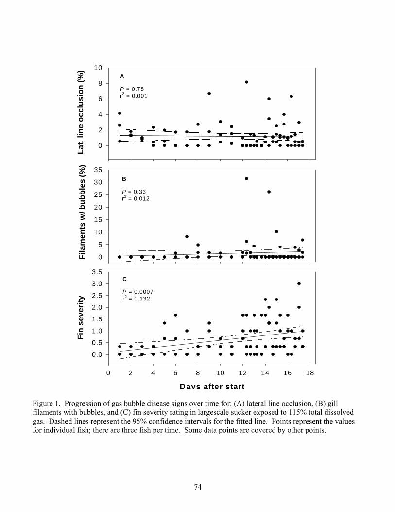
Lat.
line
occl
usio
n (%
)
0
2
4
6
8
10
Fila
men
ts w
/ bub
bles
(%)
0
5
10
15
20
25
30
35
Days after start0 2 4 6 8 10 12 14 16 18
Fin
seve
rity
0.0
0.5
1.0
1.5
2.0
2.5
3.0
3.5
A
P = 0.78r2 = 0.001
B
P = 0.33r2 = 0.012
C
P = 0.0007r2 = 0.132
Figure 1. Progression of gas bubble disease signs over time for: (A) lateral line occlusion, (B) gill filaments with bubbles, and (C) fin severity rating in largescale sucker exposed to 115% total dissolved gas. Dashed lines represent the 95% confidence intervals for the fitted line. Points represent the values for individual fish; there are three fish per time. Some data points are covered by other points.
74

Lat.
line
occl
usio
n (%
)
0
2
4
6
8
10
12
Fila
men
ts w
/ bub
bles
(log
%)
0
1
2
3
4
5
Hours after start0 2 4 6 8 10 12 14 16 18 20
Fin
seve
rity
0.0
0.5
1.0
1.5
2.0
2.5
A
P = 0.62r2 = 0.012
B
P = 0.27r2 = 0.055
C
P = 0.93r2 = 0.001
Figure 2. Progression of gas bubble disease signs over time for: (A) lateral line occlusion, (B) gill filament occlusion (Loge transformed data), and (C) fin severity rating in largescale sucker exposed to 125% total dissolved gas. Dashed lines represent the 95% confidence intervals for the fitted line. Points represent the values for individual fish; there are three fish per time. Some data points are covered by other points.
75

Days after start
0 5 10 15 20 25 30
Fin
seve
rity
0
1
2
3
Lat.
line
occl
usio
n (%
)
0
1
2
3
Fila
men
ts w
/ bub
bles
(log
%)
0
1
2
3
4
A
P = 0.023r2 = 0.060
B
P = 0.0002r2 = 0.150
C
P = 0.002r2 = 0.112
Figure 3. Progression of gas bubble disease signs over time for: (A) lateral line occlusion, (B) percent gill filaments with bubbles (Loge transformed data), and (C) fin severity rating in longnose sucker exposed to 115% total dissolved gas. Dashed lines represent the 95% confidence intervals for the fitted line. Points represent the values for individual fish; there are three fish per time. Some data points are covered by other points.
76

Hours after start0 20 40 60
Fin
seve
rity
0
1
2
3Fila
men
ts w
/ bub
bles
(log
%)
0
1
2
3
4
5
Lat.
line
occl
usio
n (%
)
0
2
4
6
8A
P = 0.60r2 = 0.006
B
P = 0.30r2 = 0.023
C
P = 0.17r2 = 0.041
Figure 4. Progression of gas bubble disease signs over time for: (A) lateral line occlusion, (B) percent gill filaments with bubbles (Loge transformed data), and (C) fin severity rating in longnose sucker exposed to 125% total dissolved gas. Dashed lines represent the 95% confidence intervals for the fitted line. Points represent the values for individual fish; there are three fish per time. Some data points are covered by other points.
77

H ours after start0 10 20 30 40 50
Fin
seve
rity
0
1
2
Lat.
line
bubb
les
(%)
0
2
4
6
8
10Fi
lam
ents
w/ b
ubbl
es (%
)
0
20
40
60
80
A
P = 0.017r2 = 0.156
B
P = 0.0003r2 = 0.326
C
P = 0.36r2 = 0.025
Figure 5. Progression of gas bubble disease signs over time for: (A) lateral line occlusion, (B) percent gill filaments with bubbles, and (C) fin severity rating in longnose sucker exposed to 130% total dissolved gas. Dashed lines represent the 95% confidence intervals for the fitted line. Points represent the values for individual fish; there are three fish per time. Some data points are covered by other points.
78
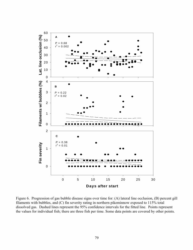
Lat.
line
occl
usio
n (%
)
0
10
20
30
40
50
60
Days after start0 5 10 15 20 25 30
Fin
seve
rity
0
1
2
Fila
men
ts w
/ bub
bles
(%)
0
1
2
3
4
A
P = 0.68r2 = 0.002
B
P = 0.22r2 = 0.02
C
P = 0.38r2 = 0.01
Figure 6. Progression of gas bubble disease signs over time for: (A) lateral line occlusion, (B) percent gill filaments with bubbles, and (C) fin severity rating in northern pikeminnow exposed to 115% total dissolved gas. Dashed lines represent the 95% confidence intervals for the fitted line. Points represent the values for individual fish; there are three fish per time. Some data points are covered by other points.
79

Lat.
line
occl
usio
n (%
)
0
10
20
30
40
50
Hours after start888 1010 121212 141414 161616 181818 202020
Fin
seve
rity
0.0
0.2
0.4
0.6
0.8
Fila
men
ts w
/ bub
bles
(%)
0
2
4
6
8
10
12
A
P = 0.78r2 = 0.004
B
P = 0.69r2 = 0.009
C
P = 0.76r2 = 0.005
Figure 7. Progression of gas bubble disease signs over time for: (A) lateral line occlusion, (B) percent gill filaments with bubbles, and (C) fin severity rating in northern pikeminnow exposed to 125% total dissolved gas. Dashed lines represent the 95% confidence intervals for the fitted line. Points represent the values for individual fish; there are three fish per time. Some data points are covered by other points.
80
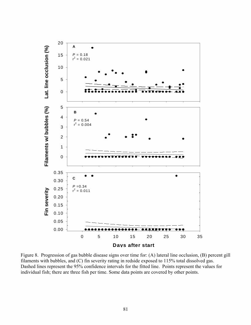
Lat.
line
occl
usio
n (%
)
0
5
10
15
20Fi
lam
ents
w/ b
ubbl
es (%
)
0
1
2
3
4
5
Days after start0 5 10 15 20 25 30 35
Fin
seve
rity
0.00
0.05
0.10
0.15
0.20
0.25
0.30
0.35
A
P = 0.18r2 = 0.021
B
P = 0.54r2 = 0.004
C
P =0.34r2 = 0.011
Figure 8. Progression of gas bubble disease signs over time for: (A) lateral line occlusion, (B) percent gill filaments with bubbles, and (C) fin severity rating in redside exposed to 115% total dissolved gas. Dashed lines represent the 95% confidence intervals for the fitted line. Points represent the values for individual fish; there are three fish per time. Some data points are covered by other points.
81

Lat.
line
occl
usio
n (%
)
05
10152025303540
Fila
men
ts w
/ bub
bles
(log
%)
0
1
2
3
4
5
Hours after start0 20 40 60 80 100
Fin
seve
rity
0
1
2
A
P = 0.19r2 = 0.017
B
P = 0.19r2 = 0.023
C
P = 0.39r2 = 0.007
Figure 9. Progression of gas bubble disease signs over time for: (A) lateral line occlusion, (B) percent gill filaments (Loge transformed data), and (C) fin severity rating in redside shiner exposed to 125% total dissolved gas. Dashed lines represent the 95% confidence intervals for the fitted line. Points represent the values for individual fish; thee are three fish per time. Some data points are covered by other points.
82

Lat.
line
occl
usio
n (lo
g %
)
0
1
2
3
4
5Fi
lam
ents
w/ b
ubbl
es (l
og %
)
0
1
2
3
4
5
Hours after start0 20 40 60 80
Fin
seve
rity
0.0
0.5
1.0
1.5
2.0
A
P = 0.13r2 = 0.03
B
P = 0.46r2 = 0.008
C
P = 0.06r2 = 0.046
Figure 10. Progression of gas bubble disease signs over time for: (A) lateral line occlusion (Loge transformed data), (B) percent gill filaments with bubbles (Loge transformed data), and (C) fin severity rating in redside shiner exposed to 130% total dissolved gas. Dashed lines represent the 95% confidence intervals for the fitted line. Points represent the values for individual fish; there are three fish per time. Some data points are covered by other points.
83

Lat.
line
occl
usio
n (%
)
20
40
60
80
r ² = 0 .29P < 0 .0001
Fila
men
ts w
/ bub
bles
(%)
0
10
20
30
40
50
r ² = 0 .003P = 0 .65
H o u rs a fter s tart0 100 200 300 400 500 600 700
Fin
seve
rity
0
1
2
r ² = 0 .05P = 0 .03
A
B
C
Figure 11. Progression of gas bubble disease signs over time for: (A) percent lateral line occlusion, (B) percent gill filaments with bubbles, and (C) fin severity rating in walleye exposed to 115% total dissolved gas. Dashed lines represent the 95% confidence intervals for the fitted line. Points represent the values for individual fish; there are three fish per time. Some data points are covered by other points.
84

Lat.
line
occl
usio
n (%
)
0
20
40
60
80
100A
P = 0.25r2 = 0.04
Fila
men
ts w
/ bub
bles
(%)
0
1
2
3B
P = 0.38r2 = 0.02
Hours after start5 10 15 20 25 30 35 40
Fin
seve
rity
0
1
2C
P = 0.22r2 = 0.05
Figure 12. Progression of gas bubble disease signs over time for: (A) percent lateral line occlusion, (B) percent gill filaments with bubbles, and (C) fin severity rating in walleye exposed to 125% total dissolved gas. Dashed lines represent the 95% confidence intervals for the fitted line. Points represent the values for individual fish; there are three fish per time. Some data points are covered by other points.
85

Lat.
line
occl
usio
n (%
)
0
20
40
60
80
100A
P < 0 .0001r2 = 0.42
Fila
men
ts w
/ bub
bles
(%)
0
1
2
3
4B
P = 0 .41r2 = 0.02
H ours after start5 10 15 20 25 30 35 40 45
Fin
seve
rity
0
1
2 C
P < 0 .002r2 = 0.18
Figure 13. Progression of gas bubble disease signs over time for: (A) percent lateral line occlusion, (B) percent gill filaments with bubbles, and (C) fin severity rating in walleye exposed to 130% total dissolved gas. Dashed lines represent the 95% confidence intervals for the fitted line. Points represent the values for individual fish; there are three fish per time. Some data points are covered by other points.
86

Hours after start0 20 40 60 80 100 120 140 160 180
Cum
ulat
ive
mor
talit
y(%
)
0
20
40
60
80
100RSS 125%LNS 125%Wal 125%RSS 130%LNS 130%WAL 130%
LT 50
Figure 14. Cumulative percent mortality for longnose sucker (LNS), walleye (WAL), and redside shiners (RSS) as a function of exposure time to 125 and 130% total dissolved gas supersaturation (TDGS). Horizontal solid line marks the point at which 50% mortality (LT50) occurred.
87

Hour0 5 10 15 20 25 30
Cum
ulat
ive
Mor
talit
y(%
)
20
40
60
80
100LSS 125% TDGSNPM 125% TDGS LSS 130% TDGS NPM 130% TDGS
LT50
Figure 15. Cumulative percent mortality for largescale sucker (LSS) and northern pikeminnow (NPM) as a function of exposure time to 125 and 130% total dissolved gas supersaturation (TDGS). Horizontal solid line marks the point at which 50% mortality (LT50) occurred.
88

Chapter III: Fishes of Rufus Woods Lake, Columbia River
D. M. Gadomski, D. A. Venditti, T. C. Robinson, J. W. Beeman, and A. G. Maule
Abstract
As a first step in aiding evaluations of possible impacts of operations at Grand Coulee Dam on fishes
below the dam, we examined fish distributions and abundances in shorelines of Rufus Woods Lake during
July 1998 and April-July 1999. During the 2-yr sampling period, 8,325 fishes representing eight families
and 21 taxa were collected during 72 h of electrofishing and 108 beach seine hauls. Eight of the species
collected were introduced, and the most abundant of these was walleye (8%). One species, rainbow trout
(14% of the catch), was mostly of net-pen origin. The majority of the catch was native species--longnose
suckers (20%), redside shiners (14%), sculpins (9%), northern pikeminnow (6%), and bridgelip and
largescale suckers (each 5-6%). The relative abundances of fish species in Rufus Woods Lake appeared to
have changed since the 1970s, when the dominant fishes were northern pikeminnow (34% of the catch),
largescale suckers (16%), peamouth (12%), and walleye (8%). This may be partly due to changes in the
seasonal hydrograph that occurred when four water storage dams were constructed on the Canadian
portion of the Columbia River during 1967-1984. Fish assemblages in Rufus Woods Lake also differed
from other Columbia River reservoirs. There are no fish passage facilities at Chief Joseph Dam, and thus
all species were resident. Because of the more northerly location of Rufus Woods Lake, we collected
species not found in the lower Columbia River, such as longnose sucker and burbot. Additionally, after
impoundment, Rufus Woods Lake remained a relatively fast-flowing system with few large backwater
areas. In contrast, many other reservoirs became more lacustrine and currently have greater abundances
of introduced taxa adapted to lentic conditions than does Rufus Woods Lake.
89

Introduction
The area of the upper Columbia River below Grand Coulee Dam, Rufus Woods Lake, has been of
concern because operations at Grand Coulee Dam could be detrimentally affecting fishes in this area. In
particular, fish kills in net pens in Rufus Woods Lake during the 1990s have been attributed to water spill
at Grand Coulee Dam causing high total dissolved gas supersaturation (TDGS) levels in the reservoir
(Elston 1998). However, little is known about populations of wild fishes in Rufus Woods Lake, and how
high TDGS levels may be affecting these species. There are few descriptions of fish abundances and
species assemblages in the upper Columbia River. Although fish assemblages in the mid and lower
Columbia River have been described (Gray and Dauble 1977, Poe et al. 1994, Barfoot et al. 2002),
conditions in these areas differ significantly from Rufus Woods Lake.
Chief Joseph Dam was completed in 1955, which changed the 83 km free-flowing reach into a river-run
reservoir (Erickson et al. 1977). Fish passage facilities were not constructed, and therefore current fish
assemblages contain only resident species. Because of the overall steep gradient of this reach and narrow
canyon morphology, much of the upper reservoir has retained more riverine characteristics than lower
Columbia River reservoirs. It has been suggested by Erickson et al. (1977) and others that short water
retention times (1.2-4.0 days) in Rufus Woods Lake might limit plankton and fish production, and thus a
major source of fish recruitment in the reservoir may be young-of-the-year fish entrained through Grand
Coulee Dam.
The only previous survey of fishes in Rufus Woods Lake was conducted during 1974-75 (Erickson et al.
1977), but conditions in the reservoir have changed since this period. In 1977, a modification of Chief
Joseph Dam raised water levels in the reservoir about 3 m. During 1967-1984, four water storage dams
on the Canadian portion of the Columbia River were constructed that altered the seasonal hydrograph
(DART River Environment 2002, Dams of the Columbia Basin 2002).
Our objective was to survey the fishes in Rufus Woods Lake as a first step in aiding evaluations of
possible impacts of dam operations. This information is also of value since it is one of the few
descriptions of fish species in a reservoir of the upper Columbia River, adding to the basic understanding
of this ecosystem. We examined fish distributions and abundances in the littoral zones of Rufus Woods
90

Lake in 1999 in relation to reservoir reach, substrate, and time period (late spring versus early summer).
To substantiate species abundances observed in 1999, results of a preliminary survey in 1998 are also
presented.
Methods
1998 Sampling. —A preliminary survey of fishes in Rufus Woods Lake was conducted during seven
nights from July 29 through August 4, 1998, using boat electrofishing and beach seining. Methods
are described in more detail below. During this period, 5-6 electrofishing sites (each receiving 10
minutes of effort) and six beach seine sites were sampled at each of five locations centered at river
kilometers (rkms) 888, 914, 939, 950, and 958, resulting in 28 electrofishing units and 30 beach seine
hauls.
1999 Substrate Mapping. —Rufus Woods Lake was divided into three reaches of approximately equal
length (Figure 1). Reach 1 extended from the Grand Coulee Dam tailrace to rkm 934, Reach 2 extended
from rkm 934 to rkm 907, and Reach 3 extended from rkm 907 to the Chief Joseph Dam forebay. The
upper reservoir (Reach 1) is characterized by higher water velocities, while the lower reservoir is more
lentic (Erickson et al. 1977). Dominant shoreline substrates were mapped along the periphery and
assigned to one of five categories based on particle diameter: sand (< 0.25 cm), gravel (0.25 to 5.1 cm),
cobble (5.1 to 25.4 cm), boulder (> 25.4 cm), and bedrock (Cummings 1962). Transition points between
substrate types were identified by visual inspection and by dragging the end of a hollow metal rod over
the substrate (Bramblett and White 2001). These transition points were recorded as waypoints in a
Trimble Pro-XR1 global positioning system (GPS) receiver and the resulting shoreline segments were
given unique identification numbers based on shoreline (north or south), reach, and substrate.
1999 Sampling. —We used a stratified random sampling design with reach and substrate as strata.
Sampling was conducted on nine consecutive nights twice each month from April through July 1999.
Sampling began about one hour before sunset and continued until approximately 0300 hours. Boat
electrofishing was the primary method of fish collection, and was conducted during each night of
sampling. Electrofishing sites were randomly selected each month in order to sample 4-6 sites per
1 Use of trade names does not imply endorsement by the United States Government.
91

substrate type in each reach. Sampling was conducted without replacement within each month, but all
sites became eligible for sampling at the start of the next month.
An electrofishing boat delivered 2 to 3 A of current to the water with 30 Hz pulsed DC at 400 to 425 V.
Shoreline segments (see substrate mapping section above) were located using a GPS on the night of
sampling and reflective markers were used to identify the upstream and downstream boundaries prior to
sampling. The entire length of shoreline segments less than 1000 m were electrofished by starting at the
upstream end and proceeding downstream. Segments greater than 1000 m long were divided for
subsampling. Segments that were 1000-1500 m in length were divided in two, and segments 1500-2500
m in length were divided into three sections; we randomly chose and electrofished one site from each of
these. Segments >2500 m were divided into 500 m sections and we randomly sampled three sites from
these. Stunned fish were immediately netted and placed in a live-well. After each segment was
electrofished, water temperature was measured.
Beach seining was conducted on two randomly selected nights during each 9-d sample period. Five beach
seine sites with sand, gravel, or cobble substrate were selected each night based on proximity to the
electrofishing sites sampled that evening. Square sets were made with a 5-mm stretch-mesh seine (30.5 m
x 2.4 m) set parallel to the shoreline. Bridal lines (6.1 m long) connected to each of the brails were used
to pull the net to shore.
Fish Identification.—Fish were lightly anesthetized in tricaine methanesulfonate (MS-222, 100 mg/l) and
generally identified to species with the exception of sculpins (Cottus spp.) and some suckers (Catostomus
spp.), which were only identified to genus. During 1998, bridgelip suckers (C. columbianus) and
largescale suckers (C. macrocheilus) were not differentiated, and were placed in an unidentified sucker
category. Also, all suckers < 150 mm fork length (FL) were placed in this category. During 1999, only
bridgelip and largescale suckers < 150 mm FL were not identified to species. Fish < 300 mm FL were
measured to the nearest 1 mm, and fish > 300 mm FL were measured to the nearest 5 mm. After
examination, fish were placed in fresh water to recover for at least 15 min before release back into the
reservoir.
92

Data Analysis. —For the data summary (Table 1), numbers of fishes collected were adjusted to
account for level of effort per shoreline substrate type, which was necessary because sampling was
not completely random. If a substrate type was sampled more or less than its actual occurrence in
reservoir shorelines, and a species preferred this substrate type, then the percent abundance of this
species would be increased or decreased over the actual value as an artifact of the stratified random
sampling plan. For example, adjusted number of carp collected during beach seining = actual
number of carp collected at sand sites x (% sand substrate in reservoir shorelines (as determined from
the shoreline substrate survey) / % sand sites sampled) + similarly adjusted numbers for other
shoreline substrate types.
For the most abundant taxa collected by each gear type in 1999, we used analysis of variance (ANOVA;
GLM procedures; SAS 1999) to test for significant effects of reach, substrate, and sampling period (April-
May versus June-July) on unadjusted catch-per-unit-effort (CPUE). Where applicable, we also divided
taxa into size groups for analysis. A unit of effort for beach seining was one haul, while for
electrofishing, a unit of effort was 10 minutes of current “on time”. Values were transformed to ln(CPUE
+ 1) for statistical comparisons. If the overall model was significant (P ≤ 0.05), Tukey’s studentized
range test was used to examine which mean transformed CPUE values differed.
Results
Environmental Variables
Reach 1 had the highest percentage of boulder substrate of all reaches, the least sand, and an intermediate
amount of cobble (Figure 1). Reach 2 was almost exclusively sand and cobble. The lowest section of
Rufus Woods Lake, Reach 3, was composed primarily of sand, gravel, and cobble.
Temperature increased steadily from 5 to 11oC during the first sampling period, April-May, and increased
from 11 to 16 oC during June-July.
93

Overview
During the 2 yr sampling period, 8,325 fishes representing 8 families and 21 taxa were collected during
72 h of electrofishing and 108 beach seine hauls (Table 1). Eight of these species were introduced. Based
on body shapes and fin condition, we determined that rainbow trout (Oncorhynchus mykiss), mainly
originated from net-pen operations in Chief Joseph and Grand Coulee reservoirs. The origin of the few
Chinook salmon (O. tshawytscha) we collected is unknown since this species is not currently stocked in
Chief Joseph or Grand Coulee reservoirs. The most abundant taxa were northern pikeminnow
(Ptychocheilus oregonensis), redside shiner (Richardsonius balteatus), three species of suckers, rainbow
trout, walleye (Stizostedion vitreum), and sculpins. We examined the catch of these species in relation to
reach, substrate, and sampling period for our primary sampling year, 1999, and for both gear types.
Except for northern pikeminnow and suckers, fishes collected by electroshocking were generally of larger
size classes and were maintained as one group per species (Figures 2 and 3). Length frequency
distributions of the most abundant species collected, longnose sucker (Catostomus catostomus), indicated
the presence of three size classes (< 150 mm, 150-299 mm, and >299 mm FL), which were separated for
analysis (Figure 4). Conversely, most fishes collected by the beach seine were of smaller sizes (Figure 5).
Electrofishing
Reach and sample period (April-May versus June-July) clearly affected CPUE of most fishes, and
distribution patterns were strongly species-specific. However, there were few significant effects of
substrate. Northern pikeminnow were collected in significantly (P < 0.01) greater numbers in Reach 3
during both time periods (Figure 2). In contrast, rainbow trout were more abundant during April-May in
Reach 1 (P < 0.01). Catches of walleye were significantly higher during April-May in all reaches, while
sculpin were significantly (P < 0.01) more abundant during June-July in Reaches 2 and 3 (Figure 2).
Larger sizes (>299 mm FL) of all three species of suckers were collected in significantly (P < 0.01)
greater numbers in Reach 1 (Figures 3 and 4). There was no significant effect of period on the abundance
of large longnose suckers, while largescale suckers were more numerous in April-May, and bridgelip
suckers more commonly collected during June-July. Substrate also significantly (P < 0.05) affected
sucker distributions, with bridgelip and largescale suckers somewhat less abundant over sand, and
conversely, longnose suckers more abundant over sand in some locations (Figures 3 and 4). There were
94
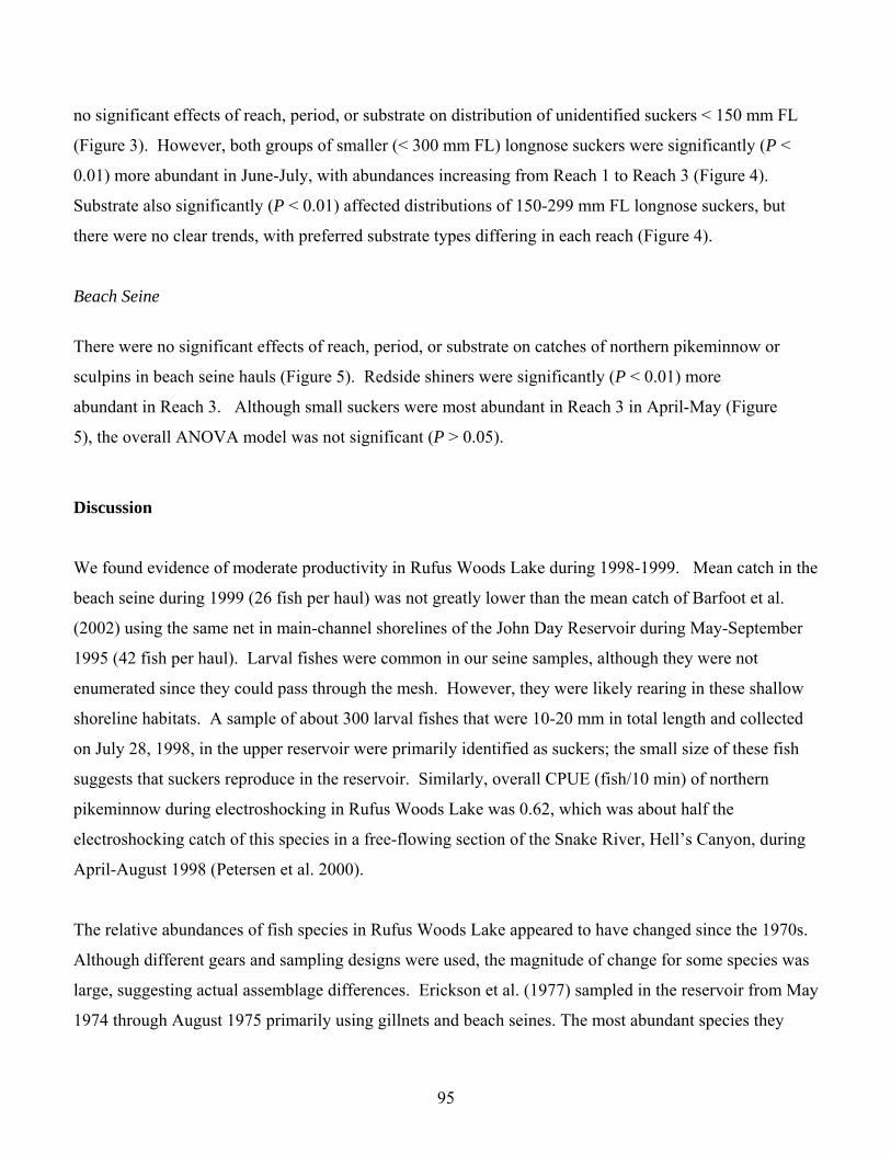
no significant effects of reach, period, or substrate on distribution of unidentified suckers < 150 mm FL
(Figure 3). However, both groups of smaller (< 300 mm FL) longnose suckers were significantly (P <
0.01) more abundant in June-July, with abundances increasing from Reach 1 to Reach 3 (Figure 4).
Substrate also significantly (P < 0.01) affected distributions of 150-299 mm FL longnose suckers, but
there were no clear trends, with preferred substrate types differing in each reach (Figure 4).
Beach Seine
There were no significant effects of reach, period, or substrate on catches of northern pikeminnow or
sculpins in beach seine hauls (Figure 5). Redside shiners were significantly (P < 0.01) more
abundant in Reach 3. Although small suckers were most abundant in Reach 3 in April-May (Figure
5), the overall ANOVA model was not significant (P > 0.05).
Discussion
We found evidence of moderate productivity in Rufus Woods Lake during 1998-1999. Mean catch in the
beach seine during 1999 (26 fish per haul) was not greatly lower than the mean catch of Barfoot et al.
(2002) using the same net in main-channel shorelines of the John Day Reservoir during May-September
1995 (42 fish per haul). Larval fishes were common in our seine samples, although they were not
enumerated since they could pass through the mesh. However, they were likely rearing in these shallow
shoreline habitats. A sample of about 300 larval fishes that were 10-20 mm in total length and collected
on July 28, 1998, in the upper reservoir were primarily identified as suckers; the small size of these fish
suggests that suckers reproduce in the reservoir. Similarly, overall CPUE (fish/10 min) of northern
pikeminnow during electroshocking in Rufus Woods Lake was 0.62, which was about half the
electroshocking catch of this species in a free-flowing section of the Snake River, Hell’s Canyon, during
April-August 1998 (Petersen et al. 2000).
The relative abundances of fish species in Rufus Woods Lake appeared to have changed since the 1970s.
Although different gears and sampling designs were used, the magnitude of change for some species was
large, suggesting actual assemblage differences. Erickson et al. (1977) sampled in the reservoir from May
1974 through August 1975 primarily using gillnets and beach seines. The most abundant species they
95

collected were northern pikeminnow (34% of the catch), largescale sucker (16%), peamouth (Mylocheilus
caurinus) (12%), and walleye (8%), with speckled dace (Rhinichthys osculus), bridgelip sucker, mountain
whitefish (Prosopium williamsoni), yellow perch (Perca flavescens), and prickly sculpin (Cottus asper)
each composing 3-5% of the catch. In contrast, the most abundant species during 1998-1999 were redside
shiners, longnose suckers, and rainbow trout (Table 1), each of which were only 1-2% of the catch in
1974-1975. The most notable declines from the mid-1970s to the late 1990s were the proportions of two
native cyprinids, peamouth and northern pikeminnow. However, it should be noted that because of
differences in sampling methodology, we cannot determine if absolute abundances of these fishes
declined.
Significant environmental changes occurred in Rufus Woods Lake from the 1960s and 1970s to the
1990s, which may have affected fish assemblage structure. The mean water level increased about 3 m
during 1977 due to dam modifications (Erickson et al. 1977). This decreased the riverine portion of the
upper reservoir, and may have increased potential down-river rearing areas. Additionally, flow patterns
differed between the two periods due to the construction during 1967-1984 of four dams on the Canadian
portion of the Columbia River (DART River Environment 2002, Dams of the Columbia Basin 2002).
These were designed to provide water storage, thus allowing regulation of seasonal flows to control
flooding and meet hydroelectric demands. Outflows from Grand Coulee Dam displayed much greater
seasonal variations during 1966-1975, reaching a 10-year average of about 7 kcms (1000 m3/sec) in June,
while in 1990-1999 the hydrograph was less variable and average flow reached a maximum of only 4.5
kcms in June (Figure 6). Changes in shoreline water level elevations were also greater during the earlier
period; yearly coefficients of daily water level variation at Chief Joseph Dam forebay were 0.15-0.45
during 1971-1975, and 0.06-0.10 during 1995-1999 (DART River Environment 2002). Temperature
regimes, however, were similar between the two periods.
The more stable conditions in Rufus Woods Lake in the 1990s may have resulted in a more productive
environment, perhaps increasing recruitment of some fishes. For example, stable conditions could have
contributed to the increase of redside shiners from the 1970s to the 1990s, since fluctuating waters levels
have been shown to reduce population densities of this species (Wydoski and Bennett 1981). Geist et al.
(1996), in a modeling exercise, determined that stable flows in Columbia River reservoirs during resident
fish spawning and rearing seasons resulted in positive benefits. High flows during late spring-early
96
summer, a common spawning period for many resident fishes, may flush eggs and larvae from protected
rearing areas. Periods of low water levels may reduce survival of eggs of shallow-spawning species such
as kokanee (O. nerka), and also disrupt benthic invertebrate prey sources (Cushman 1985). In addition,
water level fluctuations may affect shoreline habitat structure such as vegetation abundance and be
detrimental to growth and survival of age-0 fish in nursery areas (Sheidegger and Bain 1995).
Fish assemblages in Rufus Woods Lake also varied from other Columbia River reservoirs, perhaps in part
because of habitat differences due to impoundment. After impoundment, Rufus Woods Lake remained a
relatively fast-flowing system with few large backwater areas (Erickson et al. 1977). Conversely, many
other reservoirs became more lacustrine, resulting in a shift from fish assemblages composed primarily of
native riverine species to those with an abundance of introduced taxa adapted to lentic conditions (Li et al.
1987, Poe et al. 1994). For example, Barfoot et al. (2002) found that 34% of the fishes in John Day
Reservoir during 1995 were introduced, primarily sunfishes (Centrarchidae) and yellow perch, while
sunfishes remained at very low levels in Rufus Woods Lake (Table 1). Similarly, one of the few free-
flowing areas of the Columbia River, the Hanford Reach near Richland, Washington, has low abundances
of introduced fishes (Gray and Dauble 1977, Li et al. 1987). In contrast, the redside shiner, a native
cyprinid found in lotic systems, is very abundant in both the Hanford Reach and Rufus Woods Lake, but
is rare in other Columbia River impoundments (Gray and Dauble 2001, Barfoot et al. 2002).
In addition, the location of Rufus Woods Lake affected fish assemblage structure. Li et al. (1987)
presented a diagram of native fishes along a river continuum in the Pacific Northwest. They found that as
the gradient increased and water temperatures decreased, largescale and bridgelip suckers are gradually
replaced by mountain (C. platyrhynchus) and longnose suckers. Our results corroborate this model, since
we found longnose suckers to be very common in Rufus Woods Lake, while they have not been reported
further downsteam in the Columbia River (Gray and Dauble 1977, Barfoot et al. 2002). Our catch of
burbot (Lota lota) also reflects the more northerly location of Rufus Woods Lake, since this species is
very rare in the mid and lower Columbia River (Bonar et al. 2000).
Within Rufus Woods Lake, there were species and size-related differences in fish abundances, which
were primarily linked to reservoir reach. Larger sizes of some species, such as suckers, were most
abundant in upper Rufus Woods Lake, probably due in part to up-river spawning migrations. Longnose
97
suckers initiate upstream spawning migrations at 50C and continue through about 150C (Geen et al. 1966).
In the Hanford Reach of the central Columbia River, largescale suckers move upstream to spawn
primarily during June, with peak spawning at 12-150C (Dauble 1986). Similarly, we collected larger
northern pikeminnow (mean = 393 mm FL, N = 13) mostly in Reach 1 of Rufus Woods Lake, and
spawning of this species has been reported to occur in dam tailraces at temperatures > 14oC (Gadomski et
al. 2001). The higher abundances of rainbow trout in Reach 1 during April-May was probably largely due
to the location of net-pen facilities, but upriver spawning migrations of this species have also been
reported (Davies and Sloane 1987).
Conversely, although adult walleye are most abundant in upper sections of lower Columbia River
reservoirs (Beamesderfer and Rieman 1991, Zimmerman and Parker 1995), in Rufus Woods Lake they
were found in similar numbers in all reaches. This could be related to spawning distributions or forage
patterns. Walleye spawn over shallow gravel/cobble substrate in early spring when water temperatures
are about 7-9 oC (Williams and Brown 1985). Perhaps in lake-like lower Columbia River reservoirs,
walleye are restricted to spawning in tailraces with more lotic conditions and shallow depths (< 15 m),
whereas in Rufus Woods Lake, the more overall riverine environment has expanded spawning to other
reaches. Alternatively, observed distribution patterns may be related to prey availability. Walleye
aggregate below dams in lower Columbia River reservoirs and ingest outmigrating juvenile salmonids
(Poe et al. 1991), but this prey type is not available in Rufus Woods Lake.
The lower reservoir contained greater abundances of smaller fishes, probably because this area has lower
flows, smaller substrates, and more complex shoreline areas with woody debris that would offer smaller
fish refuge. Some taxa that were abundant in this area, such as sculpins and redside shiners, are smaller at
maturity. However, rearing juveniles of some species were also common. Immature longnose suckers (<
300 mm FL, and likely < 4-yrs-old; Bailey 1969) were most abundant during June-July in this area. Adult
northern pikeminnow are about 200-500 mm in length (Parker et al. 1995), and thus the fish we collected
in the lower reservoir (mean size 75 mm FL) were primarily immature.
The only species in Rufus Woods Lake that displayed significant differences in abundance due to
substrate were suckers. Adult longnose suckers were somewhat more abundant over sand substrate than
bridgelip or largescale suckers. This may be related to foraging behavior more than spawning
98

preferences, since all three species have been reported to spawn primarily over gravel substrate (McCart
and Aspinwall 1970, Dion et al. 1994). In the Hanford Reach of the middle Columbia River, both
bridgelip and largescale sucker diets are dominated by algal periphyton, which they graze from cobble
and other rock substrates (Dauble 1980, 1986). Longnose suckers have been shown to feed selectively on
cladocerans (Daphnia spp.) and chironomids, if available, in addition to algae (Brown and Graham 1954,
Barton 1980). Chironomids are commonly in fine sediment and sand substrates (Pennak 1978, Ingram
and Zieball 1983). Although Daphnia spp. are primarily pelagic, they have been reported to be ingested
by juvenile lake sturgeon (Acipenser fulvescens) over sand substrates, and it was suggested that Daphnia
spp. might be strained from sediments when they are on or near the bottom (Kempinger 1996).
Our results are one of the few descriptions of fishes in the upper Columbia River. Relative fish
abundances in Rufus Woods Lake appeared to have changed since an earlier study conducted in the 1970s
(Erickson et al. 1977), perhaps due to changes in environmental conditions during this 24-yr period.
Assemblage differences between Rufus Woods Lake and the lower Columbia River were also evident due
to both the morphology of the reservoir, and its more northerly location. Rufus Woods Lake additionally
differs from other reservoirs in the Columbia River system in that there are no fish passage facilities at
Chief Joseph and Grand Coulee dams, and therefore no upriver migration of fishes from lower reservoirs.
Because of the barriers to migration, two species we collected, rainbow trout and kokonee, were land-
locked populations of two anadromous fishes, steelhead (O. mykiss) and sockeye salmon (O. nerka),
respectively. We found that the reservoir was relatively productive. Larval fishes were present and there
were areas of juvenile rearing habitat in the littoral zone, particularly in the lower reservoir. Although
spawning was not actually documented, walleye and kokanee in spawning condition have been observed
in Rufus Woods Lake (Gregg Morris, personal communication, USGS, Cook, WA). We also collected
more large fish of some species in the upper reservoir, suggesting that upriver spawning migrations may
have been occurring.
Acknowledgments
We thank the staff of the U.S. Bureau of Reclamation Boise and Grand Coulee Dam offices, the
Confederated Tribes of the Colville Reservation, and the Columbia River Fish Farm for their cooperation
during this study. The work during this project was completed with the help of Scott VanderKooi of the
99

U.S. Geological Survey, and Sheryl Sears and Joseph Snyder of Johnson Controls World Services, Inc.
The U.S. Geological Survey and the U.S. Bureau of Reclamation jointly funded this study.
References
Bailey, M. M. 1969. Age, growth, and maturity of the longnose sucker Catostomus catostomus, of western Lake Superior. Journal Fisheries Research Board of Canada 26:1289-1299.
Barfoot, C. A., D. M. Gadomski, and J. H. Petersen. 2002. Resident fish assemblages in shallow
shorelines of a Columbia River impoundment. Northwest Science 76: 103-117.
Barton, B. A. 1980. Spawning migrations, age and growth, and summer feeding of white and longnose suckers in an irrigation reservoir. The Canadian Field-Naturalist 94:300-304.
Beamesderfer, R. C., and B. E. Rieman. 1991. Abundance and distribution of northern squawfish,
walleyes, and smallmouth bass in John Day Reservoir, Columbia River. Transactions of the American Fisheries Society 12:439-447.
Bonar, S. A., L. G. Brown, P. E. Mongillo, and K. Williams. 2000. Biology, distribution and
management of burbot (Lota lota) in Washington State. Northwest Science 74:87-96 .
Bramblett, R.G., and R.G. White. 2001. Habitat use and movements of pallid and shovelnose sturgeon in the Yellowstone and Missouri rivers in Montana and North Dakota. Transactions of the American Fisheries Society 130:1006-1025.
Brown, C. J. D., and R. J. Graham. 1954. Observations on the longnose sucker in Yellowstone Lake.
Transactions of the American Fisheries Society 83:38-46.
Cummings, K. W. 1962. An evaluation of some techniques for the collection and analysis of benthic samples with special emphasis on lotic waters. American Midland Naturalist 67: 477-504.
Cushman, R. M. 1985. Review of ecological effects of rapidly varying flows downstream from
hydroelectric facilities. North American Journal of Fisheries Management 5:330-339.
Dams of the Columbia Basin. 2002. http://www.ccrh.org/comm/river/dams9.htm.
DART River Environment. 2002. http://www.cqs.washington.edu/dart/river.html.
Dauble, D. D. 1980. Life history of the bridgelip sucker in the central Columbia River. Transactions of the American Fisheries Society 109:92-98.
Dauble, D. D. 1986. Life history and ecology of the largescale sucker (Catostomus macrocheilus) in
the Columbia River. The American Midland Naturalist 116:356-367.
100

Davies, P. E., and R. D. Sloane. 1987. Characteristics of the spawning migrations of brown trout Salmo trutta L., and rainbow trout, S. gairdneri Richardson, in Great Lake, Tasmania. Journal of Fish Biology 31:353-373.
Dion, R., M. Richardson, L. Roy, and F. G. Whoriskey. 1994. Spawning patterns and interspecific
matings of sympatric white (Catostomus commersoni) and longnose (C. catostomus) suckers from the Gouin reservoir system, Quebec. Canadian Journal of Zoology 72:195-200.
Elston, R. 1998. Fish kills in resident and captive fish caused by spill at Grand Coulee Dam in 1997:
final report. Prepared by Aquatechnics Inc., Carlsborg, Washington for the Confederated Tribes of the Colville Reservation, Nespelem, Washington and Columbia River Fish Farms, Omak, Washington.
Erickson, A. W., Q. J. Stober, J. J. Brueggeman, and R. L. Knight. 1977. An assessment of the
impact on the wildlife and fisheries resource of Rufus Woods Lake expected from the raising of Chief Joseph Dam from 946 to 956 ft. M.S.L. Unpublished report to the Colville Tribal Council, Colville Indian Reservation, and the Seattle District of the U.S. Army Corps of Engineers.
Gadomski, D. M., C. A. Barfoot, J. M. Bayer, and T. P. Poe. 2001. Early life history of the northern
pikeminnow in the lower Columbia River Basin. Transactions of the American Fisheries Society 130:250-262.
Geen, G. H., T. G. Northcote, G. F. Hartman, and C. C. Lindsey. 1966. Life histories of two species
of catostomid fishes in Sixteenmile Lake, British Columbia, with particular reference to Inlet Stream spawning. Journal of the Fisheries Research Board of Canada 23:1761-1788.
Geist, D. R., L. W. Vail, and D. J. Epstein. 1996. Analysis of potential impacts to resident fish from
Columbia River system operation alternatives. Environmental Management 20:275-288.
Gray, R. H., and D. D. Dauble. 1977. Checklist and relative abundance of fish species from the Hanford Reach of the Columbia River. Northwest Science 51:208-215.
Gray, R. H., and D. D. Dauble. 2001. Some life history characteristics of cyprinids in the Hanford
Reach, Mid-Columbia River. Northwest Science 75:122-136. Ingram, W. and C. D. Zieball. 1983. Diet shifts to benthic feeding by threadfin shad. Transactions
of the American Fisheries Society 112:554-556.
Kempinger, J. J. 1996. Habitat, growth, and food of young lake sturgeons in the Lake Winnebago system, Wisconsin. North American Journal of Fisheries Management 16:102-114.
Li, H. W., C. B. Shreck, C. E. Bond, and E. Rexstad. 1987. Factors influencing changes in fish
assemblages of Pacific Northwest streams. Pages 193-202 In W. J. Matthews and D. C. Heins (editors), Community and Evolutionary Ecology of North American Stream Fishes, University of Oklahoma Press, Norman, Oklahoma.
101

McCart, P. and N. Aspinwall. 1970. Spawning habits of the largescale sucker, Catostomus
macrocheilus, at Stave Lake, British Columbia. Journal of the Fisheries Research Board of Canada 27:1154-1158.
Parker, R. M., M. P. Zimmerman, and D. L. Ward. 1995. Variability in biological characteristics of
northern squawfish in the lower Columbia and Snake rivers. Transactions of the American Fisheries Society 124:335-346.
Pennak, R. W. 1978. Fresh-water invertebrates of the United States. John Wiley and Sons, Inc., New
York.
Petersen, J. H., C. A. Barfoot, S. T. Sauter, D. M. Gadomski, P. J. Connolly, and T. P. Poe. 2000. Predicting the effects of dam breaching in the lower Snake River on losses of juvenile salmonids to predation. Unpublished report to the U. S. Army Corps of Engineers, Walla Walla, Washington.
Poe, T. P., H. C. Hansel, S. Vigg, D. E. Palmer, and L. A. Prendergast. 1991. Feeding of predaceous
fishes on out-migrating juvenile salmonids in John Day Reservoir, Columbia River. Transactions of the American Fisheries Society 120:405-420.
Poe, T. P., R. S. Shively, and R. A. Tabor. 1994. Ecological consequences of introduced piscivorous
fishes in the lower Columbia and Snake rivers. Pages 347-360 In D. J. Stouder, K. L. Fresh, and R. J. Feller (editors), Theory and Application in Fish Feeding Ecology, University of South Carolina Press, Columbia, South Carolina.
Scheidegger, K. J., and M. B. Bain. 1995. Larval fish distribution and microhabitat use in free-
flowing and regulated rivers. Copeia 1995:125-135. Williams, K., and L. Brown. 1985. Mid-Columbia walleye—fisheries, life history, management:
1979-1982. Unpublished report to the Washington Department of Game, Olympia, Washington.
Wydoski, R. S., and D. H. Bennett. 1981. Forage species in lakes and reservoirs of the western
United States. Transactions of the American Fisheries Society 110:764-771.
Zimmerman, M.P., and R.M. Parker. 1995. Relative density and distribution of smallmouth bass, channel catfish, and walleye in the lower Columbia and Snake rivers. Northwest Science 69:19-28.
102

Table 1. Adjusted numbers of fishes collected by electroshocking (ES), and beach seining (BS) in Rufus Woods Lake during July 29-August 4, 1998, and April 4-July 28, 1999, and percent (%) catch for all gears and years combined. Gear types are combined for 1998 because of the limited sampling period. Numbers are adjusted to account for level of effort per substrate type. i = introduced species. n = primarily net pen origin. ___________________________________________________________________________________ 1998 _____1999_______ ES, BS ES BS _________ _________________ Actual number of fish collected: 865 5403 2057 Adjusted number of fish collected: 865 5671 2026 Number of hours sampled (ES) or hauls (BS): 4.7 h, 30 67.3 h 78 _____________________________________________________________________________________ Adjusted numbers 1998 1999 1999 Common name Scientific name % Catch ES, BS ES BS _____________________________________________________________________________________ Carps and minnows--Cyprinidae Carpi Cyprinus carpio 1 0 82 2 Peamouth Mylocheilus caurinus <1 5 0 19 Northern pikeminnow Ptychocheilus oregonensis 6 100 251 164 Redside shiner Richardsonius balteatus 14 50 183 937 Tenchi Tinca tinca <1 0 32 3 Unid. cyprinid <1 0 16 3 Suckers--Catostomidae Longnose sucker Catostomus catostomus 20 113 1520 82 Bridgelip sucker C. columbianus 6 -- 488 5 Largescale sucker C. macrocheilus 5 -- 409 19 Unid. catostomid 11 218 465 277 Bullhead catfishes--Ictaluridae Brown bullheadi Ameiurus nebulosus <1 0 1 0
103

Table 1. Continued. ____________________________________________________________________________________ Adjusted numbers 1998 1999 1999 Common name Scientific name % Catch ES, BS ES BS _____________________________________________________________________________________ Trouts--Salmonidae Rainbow trout n Oncorhynchus mykiss 14 103 1070 64 Kokanee O. nerka 2 1 156 10 Chinook salmon O. tshawytscha <1 1 3 1 Mountain whitefish Prosopium williamsoni 1 29 7 64 Brown trouti Salmo trutta <1 2 34 2 Bull trout Salvelinus confluentus <1 0 1 1 Brook trouti Salvelinus fontinalis <1 1 21 1 Unid. salmonid 1 0 27 21 Cods--Gadidae Burbot Lota lota 1 1 52 0 Sunfishes--Centrarchidae Smallmouth bassi Micropterus dolomieu 1 3 72 0 Perches--Percidae Yellow perchi Perca flavescens 1 8 58 4 Walleyei Stizostedion vitreum 7 49 477 38 Sculpins--Cottidae Unid. Sculpins 9 181 246 309 ____________________________________________________________________________________
104

Figure 1. Sample reaches in Rufus Woods Lake, Columbia River, Washington. Substrate composition in each reach is presented. Rkm = River kilometer.
105
0
1
2
3
4
5
6
Sculpins93 + 24 mm FL
N=253
0
1
2
3
4
5
6
Northern pikeminnow141+ 93 mm FL
N=260M
ean
CPU
E (fi
sh/1
0 m
in)
0
1
2
3
4
5
6
sandgravelcobbleboulderbedrock
ig. 2
April-May
June-July
Rainbow trout289 + 81 mm FL
N=978M
ean
CPU
E (fi
sh/1
0 m
in)
0
2
4
6
8
10
Reach
0
1
2
3
4
5
6
Walleye316 + 76 mm FL
N=442
0
1
2
3
4
5
6
0
2
4
6
8
10
April-May
June-July
Reach
0
1
2
3
4
5
6
June-July
1 2 31 2 3
1 2 3 1 2 3
Figure 2. Mean catch per unit effort (CPUE) of four taxa collectethree reaches of Rufus Woods Lake during two sample periods (Aover five substrates. CPUE is measured as fish collected per 10 mMean fork length (FL) + one standard deviation of each taxon is pNote different vertical axes scales.
106
F
d by boat electroshocking in pril-May and June-July) and inutes of current “on time”. resented. N = number of fish.
0
1
2
3
4
5
6
0
1
2
3
4
5
6
Bridgelip sucker
mea
n C
PUE
(fish
/10
min
)
0
1
2
3
4
5
6
sandgravelcobbleboulderbedrock
Fig. 3
Reach
0
1
2
3
4
5
6
April-May
June-July
Largescale sucker477 + 60 mm FL
N=440
0
1
2
3
4
5
6
Suckers < 150 mm FL82 + 28 mm FL
N=274
0
1
2
3
4
5
6469 + 91 mm FL
N=487
1 2 3 1 2 31 2 3
Figure 3. Mean catch per unit effort (CPUE) of three taxa collected by boat electroshocking in three reaches of Rufus Woods Lake during two sample periods (April-May and June-July) and over five substrates. CPUE is measured as fish collected per 10 minutes of current “on time”. Mean fork length (FL) + one standard deviation of each taxon is presented. N = number of fish.
107

0
1
2
3
4
5
6
Longnose suckers <150 mm FL
N=270
mea
n C
PUE
(fish
/10
min
)
0
1
2
3
4
5
6
Reach
0
1
2
3
4
5
6
April-May
June-July
Longnose suckers 150-299 mm FL
N=369
0
1
2
3
4
5
6Longnose suckers
>299 mm FLN=735
0
1
2
3
4
5
6
0
1
2
3
4
5
6
Fig. 4
1 2 3 1 2 3 1 2 3
sandgravelcobbleboulderbedrock
Figure 4. Mean catch per unit effort (CPUE) of three sizes of longnose suckers collected by boat electroshocking in three reaches of Rufus Woods Lake during two sample periods (April-May and June-July) and over five substrates. CPUE is measured as fish collected per 10 minutes of current “on time”. FL = Fork length. N = number of fish.
108

Fig. 5
Redside shiners54 + 12 mm FL
N=543
01020304050
Reach
01020304050
Sculpins59 + 15 mm FL
N=330
0369
1215
0369
1215
April-May
June-July
Northern pikeminnow75 + 34 mm FL
N=137
Mea
n C
PUE
0369
1215
Reach
0369
1215
April-May
June-July
April-May
June-July
05
1015202505
10152025
Mea
n C
PUE
April-May
June-July
1 2 31 2 3
sandgravelcobble
Suckers66 + 11 mm FL
N=141
1 2 31 2 3
Figure 5. Mean catch per unit effort (CPUE) of four taxa collected by beach seining in three reaches of Rufus Woods Lake during two sample periods (April-May and June-July) and over three substrates. CPUE is one beach seine haul. Mean fork length (FL) + one standard deviation of each taxon is presented. N = number of fish. Note different vertical axes scales.
109
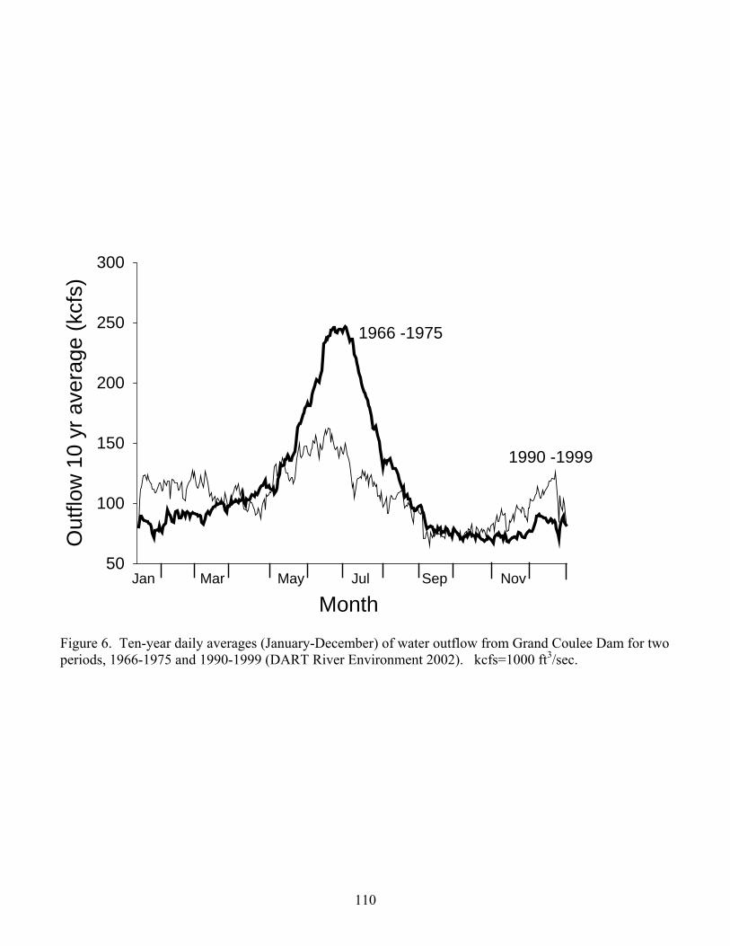
Month
Out
flow
10
yr a
vera
ge (k
cfs)
50
100
150
200
250
300
Jan May Jul NovMar Sep
1966 -1975
1990 -1999
Figure 6. Ten-year daily averages (January-December) of water outflow from Grand Coulee Dam for two periods, 1966-1975 and 1990-1999 (DART River Environment 2002). kcfs=1000 ft3/sec.
110

Chapter IV: Growth of Resident Fishes Does Not Correlate with
Years of High Gas Supersaturated Water
A. G. Maule, B. J. Adams, R. G. Morris, J. W. Beeman, and D. A. Venditti
Abstract
The growth of fish reflects the genetic capacity of the individuals, nutrition, and environmental
conditions. Environmental conditions include habitat quality and intra- and inter-specific
competition, both of which might limit the availability of food items or the ability of fish to
obtain and use food efficiently. Poor water quality such as non-optimal water temperature or
high total dissolved gas supersaturation (TDGS) can restrict growth by impacting food
availability, altering metabolism, or diverting energy resources from somatic growth to stress
responses. We examined the growth of resident fishes in Rufus Woods Lake, an impoundment of
the upper Columbia River, to see if years of high TDGS correspond to years of poor growth.
Ages of fish were determined by counting the annual growth rings (annuli) on scales from four
species collected in 1999. Incremental scale growth and fork length at capture were used to
back-calculate length-at-age. General linear models and multiple range tests were used to look
for differences in growth due to fish age and environment (year). All species had differences in
incremental scale growth based on the age of the fish—generally decreasing with age. Only
walleye had differences in growth based on the environment with 1996 growth > 1998 growth.
However, this was the opposite of what we would expect if TDGS restricted growth, as there was
much higher TDGS in 1996 than in 1998.
111

Introduction
The growth of fishes is indeterminate, meaning that, within some genetically determined limits,
growth rates of fish will increase when conditions are good and decrease when conditions are
poor (Summerfelt and Hall 1987). Ecosystem conditions that affect growth include fish density,
abundance of food, water temperature (either too hot or too cold), and other natural or
anthropogenic stresses. In most temperate aquatic systems, seasonal changes in temperature and
food availability result in rapid growth of fish in the spring and summer and reduced or no
growth in the winter. These seasonal changes in growth are reflected in growth rings on bony
structures in fish, such as otoliths and scales. Similar to the rings in trees, the annual growth
rings on fish scales can be enumerated to estimate age, and used to back-calculate growth rates in
previous years.
An environmental stressor that could potentially impact fish growth is total dissolved gas
supersaturation (TDGS). As water spills over a dam or a waterfall, it becomes mixed with
atmospheric air that can be forced into solution as the water hits the plunge-pool. If this
hydrostatic pressure caused by the plunging water is great enough it can cause TDGS, which can
lead to gas bubble disease (GBD)—a condition that can injure or kill fish. Gas bubble disease is
a non-infectious condition that affects aquatic organisms by producing emboli in blood and
tissues as well as causing other physiological stress responses (Bouck 1980, Weitkamp and Katz
1980). Fish tolerance to TDGS differs by life stages (Rucker and Kangas 1974, Weitkamp and
Katz 1980). Gas bubble disease has been reported to adversely affect the growth of fish
(Schiewe 1974, Elston 1998) by causing stress-induced lethargy, which may result in decreased
feeding (Bentley et al. 1976).
In 1996, Rufus Woods Lake, an impoundment of the Columbia River between Chief Joseph
Dam and Grand Coulee Dam, experienced TDGS > 120% during April and May (Figure 1). In
1997, TDGS reached a maximum of over 151% for one day in April, stayed between 125 to
130% for at least four days, and was above 120% for most of the period. For a three-week
period in May and June, TDGS in Rufus Woods Lake averaged over 130% and peaked at over
135% (Figure 1). Based on the presence of dead fish with obvious external signs of GBD, it
112

appears that these high-gas events caused a fish kill in Rufus Woods Lake (Elston 1998).
Surviving fish may have also experienced sublethal effects, such as reduced growth.
In 1999, as part of our study to investigate the effects of gas supersaturated water on resident fish
in Rufus Woods Lake, we collected over 7,000 fish of 21 species, and collected scales from
hundreds of the most abundant fish species. Our objectives were (1) determine the ages and
growth rates of the most abundant species in the lake by examining annual growth rings on
scales and (2) determine if the years when TDGS was high are reflected in reduced growth as
compared to years when TDGS was low.
Methods
Field collection methods in Rufus Woods Lake (rkm 877 to 960 of the Columbia River) are
described in Gadomski et al. (in press) and in Chapter III of this report and included boat
electrofishing and beach seining. We used a stratified random sampling design to collect fishes
from three reaches and five substrates ranging from sand to bedrock. Sampling was conducted
on nine consecutive nights twice each month from April through July 1999. Sampling began
about one hour before sunset and continued until approximately 0300 hours. Fish < 300 mm
fork length (FL) were measured to the nearest 1 mm, and fish > 300 mm FL were measured to
the nearest 5 mm. For each species, scales were collected for age determination from up to 10
individuals in each 5-mm length group between 30 and 600 mm FL. All scales were collected
from the left side of the fish, above the lateral line and below the dorsal fin (Dauble 1980, Jearld
1983, Maule and Horton 1985). After examination, fish were placed in fresh water to recover for
at least 15 min before release back into the reservoir. We removed scales from all species
collected; however, we limited our analyses to species for which we had readable scales from at
least 50 individuals that represented at least four year-classes. Four species met these criteria:
longnose suckers (Catostomus catostomus), northern pikeminnow (Ptychocheilus oregonensis),
rainbow trout (Oncorhynchus mykiss), and walleye (Stizostedion vitreum).
Scales were cleaned in a mild soap solution for 2 to 3 minutes and cleared of skin and debris
using a camelhair brush or a fine tipped probe. Regenerated scales—that do not have a full
113
complement of annual growth rings—were discarded at this time. Useable scales were then
rinsed in tap water, blotted dry, and mounted on gummed scale-cards. A 6.35 x 7.62 cm (2.5 x 3
inch) acetate slide was placed over the scale card and placed in a Carver laboratory press (Model
C, Fred S. Carver, Inc. Menomonee Falls, WI). The pressure was raised to 100 psi for one
minute to allow the acetate to heat to 66˚ C (150˚ F) and then increased to 6000 psi for two
minutes. Scale impressions were highlighted using a blue highlighter to improve the annulus
contrast (John Sneva, Washington Department of Fish and Wildlife, Olympia, WA, personal
communication) and examined using a microfiche reader (Devries and Frie 1996) at 24X
magnification. Annuli were interpreted as areas of compact or discontinuous circuli, which also
crossed on the anterior and lateral fields of the scale (Devries and Frie 1996). Species-specific
scale age and growth reports were used for verification of scale readings (Steinmetz and Muller
1991, Scoppettone 1988, Dauble 1980, Kisanuki 1980, Wydoski and Whitney 1979, Scott and
Crossman 1973, Alvord 1953, Scidmore and Glass 1953). Northern pikeminnow scales were
exceptional and required the use of a dichotomous key based on counting circuli to identify the
first and second annuli (Olson and Rien 1987). After the locations of annuli were determined,
the distances from the focus to each annulus and scale edge were marked on strips of paper from
which the annual change in scale radii (i.e., scale increments) were measured.
Mean annual incremental scale growth and fork length-at-ages for all species were determined
using a computer program for analyzing the growth of fish (Weisberg and Frie 1987, Weisberg
1989). The Weisberg program partitions fish growth—based on the incremental growth of
scales—to back-calculate the length of fish at different ages. We also used two-way General
Linear Models (GLM, an ANOVA for unequal sample sizes; SAS 1999) to estimate the effects
of age of the fish, the environment, and their interactions on scale growth; pairwise comparisons
were performed with Ryan-Einot-Gabriel-Welsch multiple range test (REGWQ test). Results of
statistical comparisons were considered significant when P ≤ 0.05. We also looked separately at
the second and third years of growth of each species across years. We believe this is reasonable
biologically because growth increments decreased significantly in older fish and including those
increments in the two-way GLM analyses might hide the effects of the environment on the faster
growing, younger fish. This was justified statistically because there were significant differences
in growth between ages across most year-classes.
114

The back-calculated lengths-at-age were also used to infer the age structure of the sampled
populations (Ricker 1975). Age-frequency distributions for the four fish populations were
determined for all fish collected during beach seining and electrofishing in 1999. The sizes of
these samples are listed on Figures 2 – 4 and in Gadomski et al. (in press; also see Chapter III
this report).
Results
Scales were collected from most species sampled in Rufus Woods Lake during 1999; however,
sample sizes were too low to do statistical analyses on all but four species. Back-calculated
length-at-age and population age frequency proportions were performed on longnose sucker,
northern pikeminnow, rainbow trout and walleye. Of the species collected from Rufus Woods
Lake, northern pikeminnow were the oldest—reaching 12 years of age (Figure 2)—followed by
10-year-old longnose sucker (Figure 3), 8-year-old rainbow trout (Figure 4) and 7-year-old
walleye (Figure 5).
Population year-class strength
Northern pikeminnow and rainbow trout year-class strength (frequency plots) showed that the
1998 year-classes (i.e., 1-year old fish) were not as abundant as the 1996 and 1997 year-classes
(Figures 2 and 4). The walleye frequency plot suggests that the 1997 and 1998 year-classes were
not as abundant in the population as the 1995 and 1996 year-classes (Figure 5). Longnose
suckers appeared to have an abundant 1998 year-class, but had decreased year-class strength for
1995 through 1997 (Figure 3).
Incremental scale growth
As would be expected, two-way GLM revealed significant age-effects for the incremental
growth of scales for all species (Table 1; Age, P < 0.0301). Pairwise comparisons of the scale
increments generally resulted in the expected pattern of decreasing increments with increasing
115

age (Table 2). The one exception to this was the longnose sucker in which incremental scale
growths of the age-2 and age-3 fish were significantly longer than that of age-1 fish (Table 2). It
should be noted that because we did not collect scales from 7-, 8-, or 10-year-old northern
pikeminnow, the GLM analysis of scale growth of this species was only conducted on 1-year-old
through 6-year-old fish.
Environmental effects on scale increments
Walleye was the only species to have a significant effect of the environment (i.e., year) on
incremental scale growth when we used the two-way GLM (Table 1). Scale growth in 1996—a
high gas supersaturation year—was significantly greater than in 1998—a low gas supersaturation
year—(REGWQ multiple range test, P < 0.05), but no other pairwise comparisons between years
differed (data not shown). We also looked separately at the second and third years of growth of
each species across years (Table 3). Second year scale growth of longnose suckers was greater
in 1998 than in 1993, 1994 or 1997, while third year scale growth of rainbow trout was greater in
1997 than 1996 (Table 3). The GLM analysis of walleye indicated that there were no differences
in second or third year growth (P = 0.0658); however, REGWQ pairwise (P < 0.05) comparison
indicated that second year scale growth in 1996 was greater than that in 1994 (Table 3).
Length-at-age
Incremental scale growth was used to back-calculate lengths-at-age for the year classes of the
four species. The interrelations of lengths-at-age differ from those of scale increments because
they relate the mean incremental scale growth of all individuals to each individual’s length at the
time of capture. The lengths-at-age by year class are presented for longnose sucker (Table 4),
walleye (Table 5), northern pikeminnow (Table 6), and rainbow trout (Table 7). Even though we
did not do statistical comparisons of length-at-age between year classes, we did note the percent
difference between the maximum and minimum values for each age. Maximum-minimum
differences varied between 1.5 and 12%, with northern pikeminnow and rainbow trout at the low
end (3.6% or less) and longnose sucker and walleye at the high end (up to12%).
116
Discussion
The objective of this study was to determine if we could detect reduced somatic growth in fish in
Rufus Woods Lake, and attribute the reduced growth to environmental perturbations caused by
high TDGS. Using incremental scale growth as an indicator, we found no evidence that
environmental variability influenced somatic growth of four species of fish. It is important to
note that our analyses of the growth of these fish are contingent upon several assumptions,
foremost of which is that our fish collections reflect accurately the true populations of fish in the
lake. This assumption could be violated if our collection gear failed to capture fish of a
particular size, or if we failed to sample in habitats where a significant proportion of the
population resided. We used a stratified random sampling design (Gadomski et al. in press; also
see Chapter III this report) in an attempt to collect fish from all habitats within the river, and
conducted our sampling at night. The most likely places where we could have failed to collect
fish were in the deep parts of the lake (i.e., below 4 m deep). Our work with archival depth tags
(Beeman et al.; Chapter I this report), however, suggests that at night most walleye and longnose
suckers were in shallow water where, and when, they would be vulnerable to our collection gear.
Although northern pikeminnow tended to be in deeper water in the night than in the day, they
spent over 92% of their total time in water < 5 m deep. Moreover, our samples contained many
fish, across a broad range of sizes and we believe that the populations are well represented.
We also assumed that we were able to accurately determine the locations of annuli on scales and,
thus, the ages and incremental scale growth of most of the fish we sampled. It is most likely that
this assumption would be violated when looking at scales of older fish because in older fish
somatic and scale growth slows down, which results in annuli being very close together or non-
existent (Beamish 1973). We cannot discount this possibility in the present study and it is most
likely to have happened in those species with the oldest individuals—northern pikeminnow and
longnose suckers. We did not collect individuals from some of the older northern pikeminnow
year-classes (i.e., no age 7, 8 or 10 fish; Figure 2), and the scale growth increments of age 9 and
10 longnose sucker are < 5 mm (Table 2). Despite the possibility that we failed to correctly age
the older individuals of these species, it was still appropriate to use them in our analyses because
117

we only used northern pikeminnow through age 6 and the older longnose suckers represented
fewer than 5% of the total longnose suckers in the analysis.
Analyses of variance (GLM) indicated significant differences in incremental scale growth of all
species based on the age of the fish (Table 1). For the most part this followed the expected
pattern of decreased growth as the fish aged. However, the first year incremental scale growth of
longnose suckers was significantly less than that of second and third year scale growth (Table 2).
This analysis considered the first year of scale growth for all 10 year classes (1989 through 1998)
that we identified, indicating that this difference between the first three years of scale growth was
the result of species-specific differences in behavior (e.g., a changes in feeding) or physiology
(e.g., changes in metabolism) between 1- 2- and 3-year old fish, as opposed to environmental
effects. The lack of similar differences in any of the other three species supports the
interpretation that environmental variability did not play a role in the age-specific differences in
longnose sucker scale incremental growth.
We used a GLM procedure to test for environmental effects based on differences between years
in scale growth across all ages. Of the four species considered, only walleye showed a
significant (P = 0.011) effect of the environment on incremental scale growth. Based on the
REGWQ multiple range test, there were no differences in scale growth between years, with the
exception that for all ages of walleye, their scales grew more in 1996 than in 1998. Since 1996
was a year of relatively high TDGS and 1998 had relatively low TDGS (Figure 1), the relation is
the opposite of what would be predicted if high TDGS inhibited growth. When we examined
incremental scale growth during the second and third year of growth for each species (Table 3),
we found that in only two cases did differences occur between year classes—second year growth
of longnose suckers was greater in 1998 than in 1993, 1994 and 1997, and third year growth of
rainbow trout was greater in 1997 than 1996. The longnose sucker results support the possibility
of gas supersaturation affecting growth as 1998 was a low gas year and 1997 was a high gas
year; however, the rainbow trout results do not support the possibility, as gas supersaturation was
high in both years (Table 1).
118
We also back-calculated individual fish somatic growth based on the incremental scale growth
and the length of each fish at the time of capture. We agree with Weisberg and Frie (1987), who
state that the additional variability of including fish length when calculating annual growth
makes incremental scale growth a better measure of fish growth. Nonetheless, we looked at
variability in length-at-age and found that there were as great as 12% differences in the
maximum and minimum values of length-at-age between some year classes of longnose sucker
(Table 4) and walleye (Table 5). Differences in northern pikeminnow (Table 6) and rainbow
trout (Table 7), however, were 3.6% or less.
We do not believe that the differences in length-at age—especially those for northern
pikeminnow and rainbow trout—are large enough to suggest annual environmental influences on
fish growth. It is interesting, however, to compare the growth of fish in Rufus Woods Lake to
that of fish in other areas, especially within the Columbia River Basin. Parker et al. (1995)
reported that growth of northern pikeminnow in the lower Columbia River was very similar to
that of northern pikeminnow in the lower Snake River, with both groups reaching 50, 200 and
300 mm after 1, 3, and 6 years of growth, respectively. First year growth of northern
pikeminnow in Rufus Woods Lake was comparable, but growth lagged behind populations in the
lower river by about 60% at subsequent ages (Table 6). Similarly, walleye growth in Rufus
Woods Lake was 60 to 70% less than that reported by Maule and Horton (1985) for walleye in
the lower Columbia River. To our knowledge there are no published reports on the growth of
longnose suckers in the Columbia River Basin; however, longnose suckers in the Great Slave
Lake in northern Canada (Harris 1962) grew at about the same annual rates as those reported
here but reached 19 years of age. Carlander (1969) reported the growth rates of several rainbow
trout populations in the Pacific Northwest, including the Snake River, and Scott and Crossman
(1973) reported growth rates of rainbow trout in Canada. Generally for the first two years, the
rainbow trout in Rufus Woods Lake grew at the same, or faster, rates as those reported for other
areas. However from the third to sixth years, Rufus Woods Lake fish grew at much slower rates,
so that they were about 420 mm after six years as compared to 600 to over 900 mm in many
other areas. One exception was rainbow trout in the pre-impounded Snake River, which grew at
rates very similar to those we report here. Most of the rainbow trout in Rufus Woods Lake
originated from the netpen “grow-and-release” operations in Lake Roosevelt, and we do not
119
know if there is any natural reproduction of these fish. Thus, the rapid first years of growth are
undoubtedly the result of artificial feeding prior to release.
Although the growth rates of fish in Rufus Woods Lake do not reflect annual influences of a
changing environment, such as the differences in gas supersaturation, the overall pattern of
slower growth of fish, as compared to other areas, is suggestive of an oligotrophic aquatic
ecosystem. This confirms our intuitive appraisal of the lake as a fast-water riverine system that
is cold, deep and supports slower growth than some other Columbia River reservoirs.
120

References Alvord, W. 1953. Validity of age determinations from scale of brown trout, rainbow trout and
brook trout. Transactions of the American Fisheries Society 83: 91-103. Beamish, R.J. 1973. Determination of age and growth of populations of the white sucker
(Catostomus commersoni) exhibiting a wide range in size at maturity. Journal of the Fisheries Research Board of Canada 30: 607-616.
Bentley, W. W., E. M. Dawley and T. W. Newcomb. 1976. Some effects of excess dissolved gas
on squawfish, Ptychocheilus oregonensis (Richardson). In D. H. Fickeisen and M. J. Schneider (eds.), Gas bubble disease: proceedings of a workshop held in Richland, Washington, Oct. 8-9, 1974. Energy Res. Dev. Admin., Office of Public Affairs, Tech. Inf. Center, Oak Ridge, Tennessee.
Bouck, G. R. 1980. Etiology of gas bubble disease. Transactions of the American Fisheries
Society 109:703-707. Carlander, K.D. 1969. Handbook of freshwater fishery biology. Volume 1. Iowa State University
Press, Ames. 752 pages. Dauble, D. D. 1980. Life history of the bridgelip sucker in the central Columbia River.
Transaction of the American Fisheries Society 109: 92-98. Devries, D.R. and R.V. Frie 1996. Determination of age and growth. Pages 483-512 in B.R.
Murphy and D.W. Willis, editors. Fisheries Techniques 2nd edition. American Fisheries Society.
Elston, R. 1998. Fish kills in resident and captive fish caused by spill at Grand Coulee Dam in
1997: final report. Prepared by Aquatechnics Inc., Carlsborg, Washington for the Confederated Tribes of the Colville Reservation, Nespelem, Washington and Columbia River Fish Farms, Omak, Washington.
Erickson, A. W., Q. J. Stober, J. J. Brueggeman, and R. L. Knight. 1977. An assessment of the
impact on the wildlife and fisheries resource of Rufus Woods Lake expected from the raising of Chief Joseph Dam from 946 to 956 ft. M.S.L. Report to the Colville Tribal Council, Colville Indian Reservation, and the Seattle District of the U.S. Army Corps of Engineers. University of Washington, 444 p.
Gadomski, D. M., D. A. Venditti, T. C. Robinson, J. W. Beeman, and A. G. Maule. in press.
Distribution and relative abundance of fishes in littoral areas of Chief Joseph Reservoir, Columbia River. Northwest Science 78(1).
Harris, R. H. D. 1962. Growth and reproduction of the longnose sucker, Catostomus catostomus
(Forster), in Great Slave Lake. Journal of Fisheries Research Board of Canada 19: 113-125.
121

Jearld, A., Jr. 1983. Age determination. Pages 301-324 in L.A. Nielsen and D.L. Johnson,
editors. Fisheries techniques. American Fisheries Society, Bethesda, Maryland. Joeris, L. S. 1956. Structure and growth of scales of yellow perch of Green Bay. Transactions of
the American Fisheries Society 86: 169-194. Kisanuki, T. J. 1980. Age and growth of the Humboldt sucker (Catostomus occidentalis
humboldtianus) and the golden shiner (Notemigonus crysoleucas) from Ruth Reservoir, California. Master’s thesis. Humboldt State University, Arcata, CA.
Klumb, R. A., M. A. Bozek and R. V. Frie. 1999. Proportionality of body to scale growth
validation of two back-calculation models with individually tagged and recaptured smallmouth bass and walleyes. Transactions of the American Fisheries Society 128: 815-831.
Maule, A.G., and H.F. Horton. 1985. Probable causes for the rapid growth and high fecundity
of walleye in the mid-Columbia River. Fisheries Bulletin 83(2):701-706. Montgomery, J. C. and C. D. Becker. 1980. Gas bubble disease in smallmouth bass and northern
squawfish from the Snake and Columbia Rivers. Transactions of the American Fisheries Society 109: 734-736.
Olson, D. E. and T. A. Rien. 1987. Methods of aging northern squawfish. A report to the Oregon
Department of Fish and Wildlife Dam and Hydro Studies Program Columbia River Predator-Prey Studies.
Parker, R.M., M.P. Zimmerman, and D.L. Ward. 1995. Variability in biological characteristics of
northern squawfish in the lower Columbia and Snake rivers. Transactions of the American Fisheries Society 124:335-346.
Ricker, W. E. 1975. Computation and interpretation of biological statistics of fish populations.
Fisheries Research Board of Canada Bulletin 191. Rucker, R. R. and P. M. Kangas. 1974. Effect of nitrogen supersaturated water on coho and
Chinook salmon. The Progressive Fish-Culturist 36: 152-156. SAS (Statistical Analysis System). 1999. SAS Proprietary Software Release 8.1. Copyright
1999-2000 by SAS Institute Inc., Cary, North Carolina, USA. Scidmore, W. J. and A. W. Glass 1953. Use of pectoral fin rays to determine age of the white
sucker. The Progressive Fish-Culturist 15: 114-115. Schiewe, M. H. 1974. Influence of dissolved atmospheric gas on swimming performance of
juvenile Chinook salmon. Transactions of the American Fisheries Society 103: 717-721.
122

Scoppettone, G. G. 1988. Growth and longevity of the cui-ui and longevity of other catostomids and cyprinids in western North America. Transactions of the American Fisheries Society 117: 301-307.
Scott, W. B. and E. J. Crossman. 1973. Freshwater fishes of Canada. Bulletin 184 Fisheries
Research Board of Canada, Ottawa. Steinmetz, B. and R. Muller. 1991. Atlas of fish scales and other bony structures used for age
determination non-salmonid species found in European fresh waters. Samara Publishing, Tresaith, Great Britain.
Summerfelt, R.C. and G.E. Hall (editors). 1987. Age and growth of fish. Iowa State University
Press, Ames. 544 pages. Toothaker, L. E. 1993. Multiple comparison procedures. Sage University paper series on
quantitative applications in the social sciences, 07-089. Newbury Park, CA; Sage. Weisberg, S. and R. V. Frie. 1987. Linear models for the growth of fish. Pages 127-143 in R. C.
Summerfelt and G. E. Hall, editors. Age and growth of fish. Iowa State University Press, Ames.
Weisberg, S. 1989. A computer program for analyzing the growth of fish. Published by the
Minnesota Sea grant College Program. University of Minnesota. 16 p. Weitkamp, D. E. and M. Katz. 1980. A review of dissolved gas supersaturation literature.
Transactions of the American Fisheries Society 109:659-702. Wydoski, R. S. and R.R. Whitney. 1979. Inland fishes of Washington. University of Washington
Press. Seattle and London.
123

Table 1. Results of two-way analyses of variance of growth of four species of fish from Rufus Woods Lake. Analyses considered scale increments as a surrogate for fish growth and examined variation due to age (for example, differences in incremental scale growth of 1-year old fish as opposed to 2-year old fish independent of the year) and year (i.e., environment; for example, differences in 1-year old fish based on the year).
Northern pikeminnow
Source df MS F P Age 5 225.6 11.32 <0.0001 Year/Environment 5 1.6 0.08 0.9952 Interaction 10 21.5 1.08 0.3809 Error 159 19.9
Longnose sucker
Source df MS F P Age 9 2378.7 43.95 <0.0001 Year/Environment 9 101.8 1.88 0.0516 Interaction 36 65.5 1.21 0.1877 Error 782 54.1
Walleye
Source df MS F P Age 6 4626.7 57.45 <0.0001 Year/Environment 6 224.8 2.79 0.0111 Interaction 15 117.2 1.46 0.1172 Error 505 89.5
Rainbow trout
Source df MS F P Age 7 104.5 2.24 0.0301 Year/Environment 7 20.1 0.43 0.8826 Interaction 21 63.4 1.36 0.1333 Error 459 46.7
124
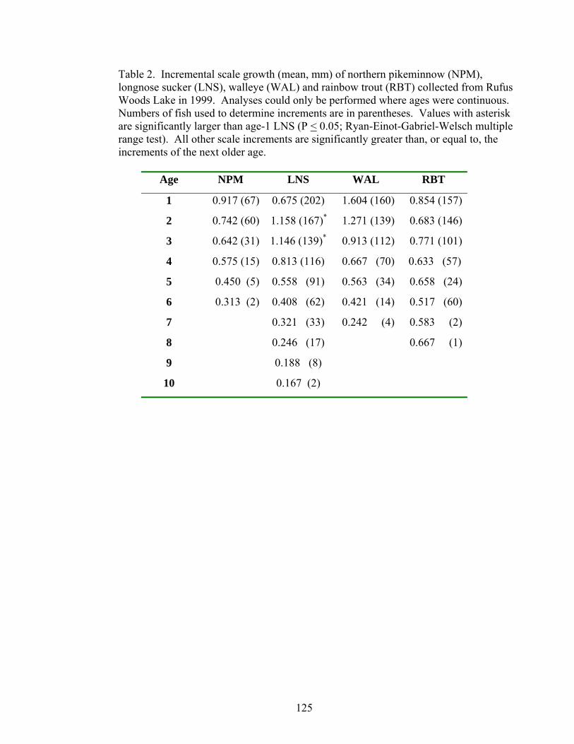
Table 2. Incremental scale growth (mean, mm) of northern pikeminnow (NPM), longnose sucker (LNS), walleye (WAL) and rainbow trout (RBT) collected from Rufus Woods Lake in 1999. Analyses could only be performed where ages were continuous. Numbers of fish used to determine increments are in parentheses. Values with asterisk are significantly larger than age-1 LNS (P < 0.05; Ryan-Einot-Gabriel-Welsch multiple range test). All other scale increments are significantly greater than, or equal to, the increments of the next older age.
Age NPM LNS WAL RBT
1 0.917 (67) 0.675 (202) 1.604 (160) 0.854 (157)
2 0.742 (60) 1.158 (167)* 1.271 (139) 0.683 (146)
3 0.642 (31) 1.146 (139)* 0.913 (112) 0.771 (101)
4 0.575 (15) 0.813 (116) 0.667 (70) 0.633 (57)
5 0.450 (5) 0.558 (91) 0.563 (34) 0.658 (24)
6 0.313 (2) 0.408 (62) 0.421 (14) 0.517 (60)
7 0.321 (33) 0.242 (4) 0.583 (2)
8 0.246 (17) 0.667 (1)
9 0.188 (8)
10 0.167 (2)
125

Table 3. Results of one-way general linear model (GLM) and Ryan-Einot-Gabriel-Welsch (REGWQ) pair-wise comparison of age-specific growth of four species of fish from Rufus Woods Lake—northern pikeminnow (NPM), longnose sucker (LNS), walleye (WAL) and rainbow trout (RBT). Analyses were done independently on each age across year-classes in which our sample size was > 10. The number of year-classes used in the analysis is equal to the degrees of freedom (df) plus one.
Species Age (years)
n df F P
NPM 2 55 2 0.20 0.8193
3 26 1 0.89 0.3548
LNS 2 150 5 4.81 0.00041
3 122 4 0.62 0.6502
WAL 2 135 4 2.26 0.06582
3 108 3 0.54 0.6554
RBT 2 139 3 0.66 0.5811
3 94 2 4.23 0.01753
1 – 1998 year class > 1993, 1994, 1997 and = 1995 and 1996 year classes 2 – although GLM was not significant, 1996 year class > 1994 year class based on
REGWQ pairwise comparison 3 – 1997 year class > 1996 = 1998 year class
126

Table 4. Mean back-calculated length-at-age measurements (mm) and ±1 SE (in parentheses) for annual year classes of longnose sucker in Rufus Woods Lake collected in 1999. Percent difference (% Diff) between minimum and maximum length-at-age is shown for all ages with more than two year classes. Only those year classes with sample sizes > 2 were used in this analysis.
Year Class Age (Years)
% Diff 1998 1997 1996 1995 1994 1993 1992 1991 1990 1989
1 11.7 97.60 (1.14)
92.76 (1.11)
94.63 (1.26)
94.91 (1.21)
89.75 (1.06)
87.87 (1.07)
86.62 (1.50)
86.19 (2.19)
91.93 (3.24)
94.83 (8.92)
2 9.9 173.31 (1.84)
170.35(2.01)
172.50(1.75)
167.63(1.75)
160.58(1.75)
157.44 (2.40)
155.77 (4.62)
161.08 (4.62)
169.72 (11.07)
3 10.4 234.36(2.58)
231.67(2.46)
228.67(2.23)
221.90(2.24)
213.61 (3.01)
210.04 (5.56)
214.11 (5.56)
222.32 (12.48)
4 10.0 293.47(2.77)
285.63(2.49)
280.74(2.52)
272.72 (3.41)
264.00 (4.66)
266.18 (6.15)
273.14 (13.32)
5 8.0 339.39(2.66)
329.65(2.68)
323.51 (3.64)
315.17 (4.96)
312.09 (6.48)
317.16 (13.82)
6 5.6 362.19(2.58)
351.21 (3.85)
344.64 (5.27)
341.94 (6.86)
341.86 (14.35)
7 3.2 385.24 (4.33)
373.83 (7.19)
373.00 (7.58)
373.19 (15.44)
8 1.5 383.35 (6.84)
377.68 (8.71)
379.75 (17.18)
9 421.49 (10.09)
418.72 (19.29)
10 447.98 (27.80)
127

Table 5. Mean back-calculated length-at-age measurements (mm) and ±1 SE (in parentheses) for annual year classes of walleye in Rufus Woods Lake collected in 1999. Percent difference (% Diff) between minimum and maximum length-at-age is shown for all ages with more than two year classes. Only those year classes with sample sizes > 2 were used in this analysis.
Year Class Age (Years)
% Diff 1998 1997 1996 1995 1994 1993 1992
1 10.1 176.63 (3.20)
173.13 (2.89)
176.94 (2.37)
171.06 (2.48)
166.45 (3.26)
162.16 (4.59)
158.98 (7.83)
2 11.8 246.46 (3.88)
246.77 (3.11)
244.71 (3.34)
234.21 (4.33)
225.31 (6.04)
217.84 (9.99)
3 12.0 325.65 (3.54)
320.09 (3.76)
313.41 (4.98)
298.63 (6.87)
286.55 (11.18)
4 10.9 359.20 (4.14)
349.03 (5.45)
338.06 (7.64)
320.10 (12.26)
5 7.5 386.70 (6.08)
372.24 (8.50)
358.09 (13.68)
6 377.03 (9.81)
359.39 (15.67)
7 425.54 (20.26)
128
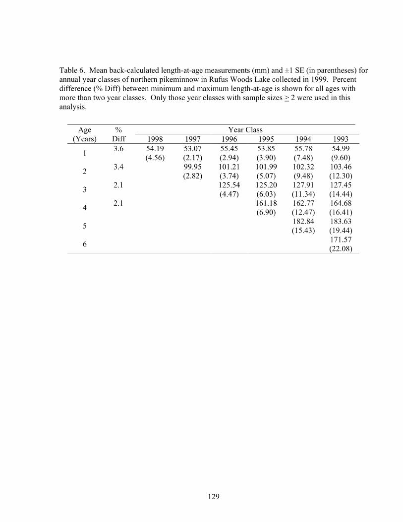
Table 6. Mean back-calculated length-at-age measurements (mm) and ±1 SE (in parentheses) for annual year classes of northern pikeminnow in Rufus Woods Lake collected in 1999. Percent difference (% Diff) between minimum and maximum length-at-age is shown for all ages with more than two year classes. Only those year classes with sample sizes > 2 were used in this analysis.
Year Class Age (Years)
% Diff 1998 1997 1996 1995 1994 1993
1 3.6 54.19 (4.56)
53.07 (2.17)
55.45 (2.94)
53.85 (3.90)
55.78 (7.48)
54.99 (9.60)
2 3.4 99.95 (2.82)
101.21 (3.74)
101.99 (5.07)
102.32 (9.48)
103.46 (12.30)
3 2.1 125.54 (4.47)
125.20 (6.03)
127.91 (11.34)
127.45 (14.44)
4 2.1 161.18 (6.90)
162.77 (12.47)
164.68 (16.41)
5 182.84 (15.43)
183.63 (19.44)
6 171.57 (22.08)
129
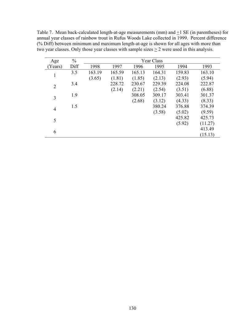
Table 7. Mean back-calculated length-at-age measurements (mm) and +1 SE (in parentheses) for annual year classes of rainbow trout in Rufus Woods Lake collected in 1999. Percent difference (% Diff) between minimum and maximum length-at-age is shown for all ages with more than two year classes. Only those year classes with sample sizes > 2 were used in this analysis.
Year Class Age (Years)
% Diff 1998 1997 1996 1995 1994 1993
1 3.5 163.19 (3.65)
165.59 (1.81)
165.13 (1.85)
164.31 (2.13)
159.83 (2.93)
163.10 (5.94)
2 3.4 228.72 (2.14)
230.67 (2.21)
229.39 (2.54)
224.08 (3.51)
222.87 (6.88)
3 1.9 308.05 (2.68)
309.17 (3.12)
303.41 (4.33)
301.37 (8.33)
4 1.5 380.24 (3.58)
376.88 (5.02)
374.39 (9.59)
5 425.82 (5.92)
425.73 (11.27)
6 413.49 (15.13)
130

90
100
110
120
130
140
150
160
6-Apr
13-A
pr20
-Apr
27-A
pr4-M
ay11
-May
18-M
ay25
-May
1-Jun
8-Jun
15-Ju
n22
-Jun
29-Ju
n6-J
ul13
-Jul
20-Ju
l27
-Jul
3-Aug
10-A
ug
TDG
(%)
1996 1997 1998 1999
Figure 1. Total dissolved gas (TDG; % saturation) in Rufus Woods Lake in the spring and summer, 1996 through 1999. Data from US Army Corps of Engineers.
131

Northern pikeminnowN = 326
0
10
20
30
40
50
60
1998 1996 1994 1992 1990 1988Year Class
Freq
uenc
y (%
)
Figure 2. Frequencies of year classes of northern pikeminnow in Rufus Woods Lake, 1999.
132
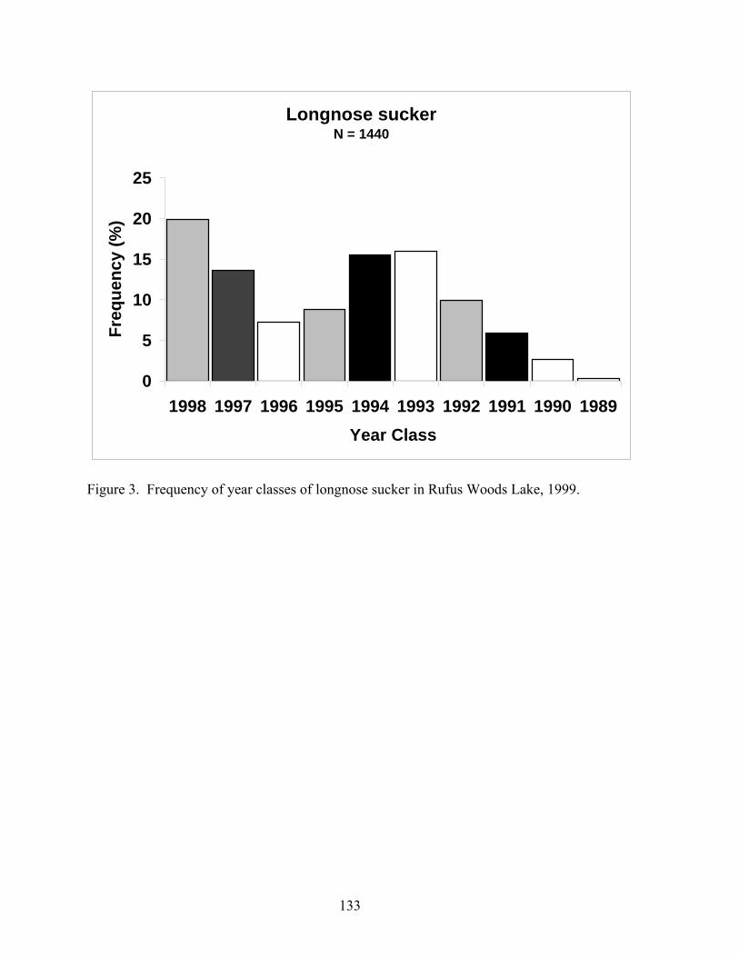
Longnose suckerN = 1440
0
5
10
15
20
25
1998 1997 1996 1995 1994 1993 1992 1991 1990 1989Year Class
Freq
uenc
y (%
)
Figure 3. Frequency of year classes of longnose sucker in Rufus Woods Lake, 1999.
133
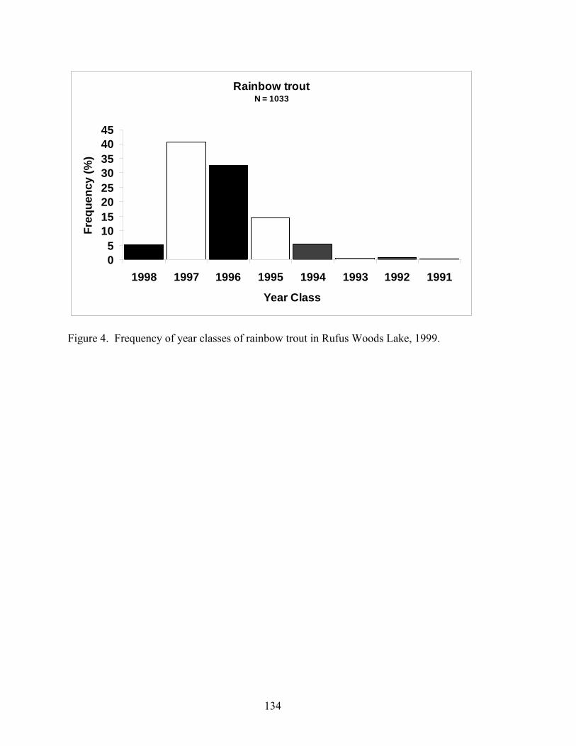
Rainbow troutN = 1033
05
1015202530354045
1998 1997 1996 1995 1994 1993 1992 1991
Year Class
Freq
uenc
y (%
)
Figure 4. Frequency of year classes of rainbow trout in Rufus Woods Lake, 1999.
134

WalleyeN = 465
0
5
10
15
20
25
30
35
1998 1997 1996 1995 1994 1993 1992
Year Class
Freq
uenc
y (%
)
Figure 5. Frequency of year classes of walleye in Rufus Woods Lake, 1999.
135
Chapter V: Lateral line pore diameters correlate with the
development of gas bubble trauma signs in several Columbia River
fishes
R. G. Morris, J. W. Beeman, S. P. VanderKooi and A. G. Maule. Abstract Gas bubble trauma (GBT) caused by gas supersaturation of river water continues to be a problem
in the Columbia River Basin. A common indicator of GBT is the percent of the lateral line
occluded with gas bubbles; however, this effect has never been examined in relation to lateral
line morphology. The effects of 115%, 125%, and 130% total dissolved gas levels were
evaluated on five fish species common to the upper Columbia River. Trunk lateral line pore
diameters differed significantly (P < 0.0001) among species (longnose sucker >largescale sucker
> northern pikeminnow > Chinook salmon > redside shiner). At all supersaturation levels
evaluated, percent of lateral line occlusion exhibited an inverse correlation to pore size but was
not generally related to total dissolved gas level or time of exposure. This study suggests that the
differences in lateral line pore diameters between species should be considered when using
lateral line occlusion as an indicator of gas bubble trauma.
136

Introduction
Gas bubble trauma (GBT) or gas bubble disease has re-emerged as an issue in the Columbia
River Basin in part due to the listing of salmonid runs under the Endangered Species Act
(http://www.nwr.noaa.gov). Listing salmonids has caused the dams on the Columbia and Snake
rivers to release extra water to aid in smolt migration. This has resulted in increases in total
dissolved gas supersaturation (TDGS) levels due to gas entrainment by water plunging into these
rivers from spillways or other release points (US Army Corps of Engineers 2000).
Total dissolved gas supersaturation has been proven to be hazardous to fish resulting in GBT
(Marsh and Gorham 1905, Ebel 1971, Ebel et al. 1975, Weitkamp and Katz 1980, Krise and
Herman 1991, Mesa and Warren 1997, Counihan et al. 1998, Mesa et al. 2000, Ryan et al. 2000).
Gas bubble trauma (disease), as defined by Bouck (1980), is “a non-infectious, physically
induced process caused by uncompensated, hyperbaric total dissolved gas pressure, which
produces primary lesions in blood (emboli) and in tissues (emphysema) and subsequent
physiological dysfunctions”. Signs of GBT typically include bubbles in the eyes, fins, skin,
lateral line and gill filaments, hemorrhaging and exophthalmia (popeye). Methods for evaluating
GBT in salmonids and other species typically include examining the eyes, fins, skin, gular
palette and the lateral line for bubble formation (Ebel 1971, Ebel et al. 1975, Weitkamp and Katz
1980, Mesa and Warren 1997, Ryan et al. 2000, Mesa et al. 2000). The signs of GBT are highly
variable; Ryan et al. (2000) investigated the effects of TDGS on over 25 species of non-salmonid
fishes from the Columbia and Snake Rivers and found a positive correlation between the
incidence and severity of GBT and TDGS. However, they concluded that the high variability in
GBT signs precluded creating an accurate model relating TDGS to mortality.
The accepted function of the lateral line canal is that of a “mechano-sensory” organ (Dijkgraaf
1967, Coombs and Montgomery 1999). However, bubbles in the lateral line (lateral line
occlusion) have been routinely evaluated as an index of GBT (Ebel 1971, Dawley and Ebel
1975, Ebel et al. 1975, Stroud et al. 1975, Fickeisen and Montgomery 1978, Montgomery and
Becker 1980, Nebeker et al. 1980, Krise and Herman 1991, Mesa and Warren 1997, Hans et al.
1999, Mesa et al. 2000) and lateral line bubbles are typically the first signs of GBT observed in
fish (Weitkamp and Katz 1980). The assumptions for these evaluations being that the
137

morphology of the lateral line is identical regardless of fish size, the lateral line pores are the
same size in all species, and that lateral line morphology plays no role in the expression of GBT
signs. Weber and Schiewe (1976) evaluated lateral line morphology and function of juvenile
steelhead trout in relation to GBT, but their study was focused on the changes in response
capability of the lateral line due to gas bubble formation.
The function and morphology of the lateral line have been evaluated in many species
(Jakubowski 1966,1966A, 1967, 1974, Montgomery et al. 1994, Janssen et al. 1999). Janssen et
al. (1999) measured the diameter of lateral line pores on the heads of sculpin and their potential
effects on prey sensing ability but they did not measure trunk lateral line pore diameters. Lateral
line pore morphology and its potential significance to lateral line sensory function, GBT lateral
line bubble formation, and gas bubble retention, and species-specific differences are unknown.
Krise and Herman (1991) reported observing bubbles in the lateral line pores due to TDGS in
juvenile Atlantic salmon Salmo salar but not in lake trout Salvelinus namaycush in the same
system; however, they did not investigate the issue further.
Resident fish populations from Rufus Woods Lake (also known as Chief Joseph Reservoir) have
exhibited shifts in species composition and dominance from the 1970s (Erickson et al. 1977) to
1999 (Venditti et al. 1999, Gadomski et al. in press), possibly in response to hydropower
operations, including TDGS events. In particular, Venditti et al. (1999) and Gadomski et al. (in
press; also see Chapter 3 of this report) found that sucker populations exhibited shifts in
community structure and species dominance. The order of abundance reversed between 1970
and 1999 with longnose sucker (Catostomus catostomus), shifting from very small numbers to
numeric dominance over largescale (C. macrocheilus) and bridgelip suckers (C. columbianus)
with suckers accounting for 41.5% of the total fish observed (Venditti et al. 1999). It was also
noted that some size classes of bridgelip and largescale suckers appeared to be absent (or present
in very small numbers).
Laboratory GBT studies were conducted at the Columbia River Research Laboratory (CRRL)
examining gas bubble trauma effects on fish resident to Rufus Woods Lake, attempting to
determine if species exhibited differences in TDGS sensitivity. Systematic evaluation of pore
138

sizes was initiated when obvious differences in trunk lateral line occlusion and pore sizes
between species were observed. The objectives of this study were to determine (1) if trunk
lateral line pore diameters differed between species, location on the lateral line or between fish of
different lengths and (2) if there was a correlation between lateral line pore diameter and lateral
line occlusion when fish were exposed to TDGS. Lateral line pore diameters were evaluated for
four species common in this reservoir - largescale sucker, longnose sucker, northern pikeminnow
(Ptychocheilus oregonensis), and redside shiner (Richardsonius balteatus). Yearling Chinook
salmon (Oncorhynchus tshawytscha) were also evaluated for comparative purposes, as they
exhibited up to 30% occlusion at 110% TDGS when tested by Mesa et al. (2000). Trunk lateral
line pore sizes were not evaluated in their study or in any other previous GBT study.
Methods Laboratory GBT trials were conducted at CRRL, Cook, WA, from May 2000 to April 2001.
Well water with the following water quality characteristics was used for all testing: hardness <
10 mg/L; alkalinity (total as CaCO3) = 20 mg/L; pH = 6.6. National Testing Laboratories LTD,
Cleveland, OH, conducted chemical analysis of the well water for water quality analysis and
potential contaminants according to EPA approved methods for particular compounds or
Standard Methods. These analyses were conducted to drinking water standards and scans
included: metals, fluoride, chloride, nitrite, nitrate, sulfate, total dissolved solids, turbidity,
trihalomethanes, pesticides and PCBs.
Experimental system —This experimental system followed the design used by Mesa et al.
(2000). Supersaturated water was generated by injecting atmospheric air into heated water under
pressure. The treatment tanks had a mean water depth (± SE) of 26.0 ± 0.1 cm to minimize
depth compensation and a mean water volume of 154.8 ± 2.5 L. Target water temperature for all
studies was 12.0 ºC (for specific study values see Table 1). The system had a one-time flow-
through design with a mean flow rate of 4.8 ± 0.1 L/min per tank. Factors measured which
affect TDGS included water temperature, barometric pressure, barometric pressure minus total
pressure (∆ P), and percent saturation. These factors were monitored throughout all studies
using a Total Dissolved Gas and Oxygen Monitor, Model TBO-L (Common Sensing, Inc., Clark
Fork, ID). In order to compensate for gas instability, the meter’s probe was placed near the
139
bottom of a vertical 3-m long, clear PVC tube plumbed in parallel with the system. Nominal
TDGS concentrations were also measured in all tanks before and after each trial (Table 1) using
the Common Sensing TDGS meter, a Weiss ES-2 Saturometer (Eco Enterprises, Seattle, WA) or
Tensionometer 300E (Alpha Designs, Victoria, B.C.). Different meters were used due to meter
malfunctions and all meters were calibrated according to the manufacturer’s specifications. We
dealt with gas instability in the water and sensor membrane bubble formation by gently sweeping
the gas probes in a circular motion for five-minutes before taking the readings in each tank.
Fish collection and handling —Fish used in this study were largescale sucker (N = 67, mean
weight (WT) ± SE = 30.0 ± 0.1 g, mean fork length (FL) ± SE = 136.7 ± 0.1 mm), longnose
sucker (N = 28, WT = 71.1 ± 2.5 g, FL = 180.8 ± 1.8 mm), northern pikeminnow (N = 75, WT =
34.6 ± 2.3 g, FL = 137.1 ± 2.7 mm), Chinook salmon (N = 75, WT = 15.8 ± 1.2 g, FL = 123.5 ±
3.4 mm) and redside shiner (N = 27, WT = 8.2 ± 0.1 g, FL = 87.7 ± 0.1 mm). The study fish,
with the exception of the Chinook salmon (see below), were collected from Rufus Woods Lake
(the reservoir between Chief Joseph and Grand Coulee dams) and the Hanford Reach of the
Columbia River in the spring and summer of 2000 and returned to CRRL for study. Fish were
collected by boat electrofisher (Smith-Root 18-E Electrofishing Workboat, Model GPP
Electrofisher, Vancouver, WA) using 400-500 V pulsed DC at 30 pulses/sec and 3-4 Amps. Fish
were netted and placed in a live well then held in 133-L mesh-walled containers in the river or in
a small concrete raceway supplied with well water for up to 2 days prior to transportation to
CRRL. Yearling hatchery fall Chinook salmon were obtained from the Abernathy Fish
Technology Center, Longview, WA, (brood stock 2000).
All test fish were held in outdoor 1,400-L flow-through circular fiberglass holding tanks and
were acclimatized to 12° C well water for a minimum of one week prior to testing. Holding
tanks and the control tanks used heated water from the same source. All water used in these
experiments was first allowed to cascade through a column (66 cm tall by 18 cm diameter)
packed with one-inch bio-barrels to remove any excess dissolved gas due to water heating. Fish
were fed Deep-frozen Blood Worms™ (redside shiner) or Rangen Quality Feed for
Aquaculture™ (Chinook salmon, both sucker species and northern pikeminnow) daily. Fish were
maintained under a natural photoperiod and were not fed during individual trials.
140
Experimental protocols— To create signs of GBT, fish were exposed to 115, 125 and 130%
TDGS as described by Mesa et al. (2000). At the beginning of an experiment, fish were stocked
into four treatment tanks in which the water was at the pre-determined TDGS level (Table 1),
and two control tanks. As soon as the first mortality was noted, we began sampling every 2 h
until all treatment fish had been sampled or had died. At sampling, fish were netted within 5 sec
of opening the tank lid and placed in a lethal dose of buffered tricaine methanesulfonate (MS-
222; 200 mg/L). The MS-222 solution was prepared from water with TDGS equal to that of the
tank. We do not believe this sampling protocol affects signs of GBT and it has been used
extensively in similar research (Mesa and Warren 1997, Hans et al. 1999, Mesa et al. 2000).
Evaluation of GBT included examining the unpaired fins, the eyes, and the gills (data not
included here) as well as the lateral line for bubbles. Bubbles in the trunk lateral line were
quantified using a dissecting microscope with 8-40X-zoom magnification. A micrometer with
0.5 mm gradations was laid along side of the trunk lateral line to determine the proportion of its
length occluded with bubbles (expressed as percent). An exception to this protocol was Chinook
salmon, which were only evaluated to compare development of bubbles in the lateral line. In
separate experiments, juvenile Chinook salmon were exposed to 125 and 130% TDGS (20 fish in
each of two treatment and one control tanks) and were examined for lateral line occlusion hourly
for 5 h.
Trunk lateral line pore diameters were measured at 25X or 40X magnification using a calibrated
ocular micrometer. Pore diameters were always measured horizontally along the axes of the fish.
Three pores per fish were measured -- the first measurable pore adjacent to the gill operculum,
one pore at the midpoint of the body near the dorsal fin, and one adjacent to the caudal fin.
Data analysis — The relationship between lateral line occlusion and TDGS exposure was
evaluated using General Linear Models or linear regression. Since these data were percentage
data, arcsine transformation was conducted and comparisons of means were accomplished using
General Linear Models (GLM, SAS 1999) and the Ryan’s (Ryan-Einot-Gabriel-Welsch,
REGWQ) multiple range tests (MRT, α = 0.05). Data were not collected from mortalities
because the exact time of death and its effect on lateral line bubble retention was not known.
141

The relationships between fork length and trunk lateral line pore diameter were also evaluated
using General Linear Models and Ryan’s MRT. Ryan’s MRT also was used to compare pore
diameters at the three locations pores were measured on the fish. During some trials lateral line
occlusion changed through time of exposure (i.e., longnose sucker in 115% and 130% TDGS and
Chinook salmon in 125 and 130% TDGS), nonetheless, we pooled data within these trials to get
exposure-specific measures of bubble formation in the lateral lines of the five species we
examined.
Results
Water Quality
The TDGS levels were generally successfully maintained at the desired level throughout the
exposures (Table 1). TDGS levels in treatment tanks were calibrated to the airflow to the
system, which was regularly monitored before and during the studies. This insured the
constancy of tank gas levels and allowed us to use data where only one tank gas level was
measured. The TDGS in control tanks was consistent for all studies and maintained at 104.3 ±
0.1%; N = 50 and no water quality problems were detected in our testing water.
Largescale sucker
Mean levels of lateral line occlusion were significantly lower in fish exposed to 115% TDGS
than at 125% (N = 171, F = 21.9, P< 0.0001; Figure 1). Mean lateral line pore width for
largescale suckers was 0.18 ± 0.01 mm and the slope for the regression line of fork length to pore
width did not differ significantly from zero (Figure 2a, N = 59, F = 1.48, P= 0.23, r2 = 0.03).
There was no significant difference between lateral line pore diameters measured at different
locations on the lateral line (Table 2) and the pores were uniformly oval.
142
Longnose sucker
Mean lateral line occlusion was significantly lower at 115% than 125 or 130% TDGS (N = 274,
F = 13.6, P< 0.0001; Figure 1). There was no significant difference between mean lateral line
occlusion at 125 and 130% TDGS. On many specimens, GBT was characterized by bead-like
rows of bubbles in the mucous directly above trunk lateral line pores. Bubbles were observed
exiting these pores on several occasions in this species but not in other species used in these
studies.
Mean lateral line pore diameter of longnose suckers was 0.49 ± 0.01 mm. The slope for the
regression line of fork length to pore width did not differ significantly from zero (N = 27, F =
0.3, P= 0.62, r2 = 0.01, Figure 2a). Lateral line pore diameters decreased slightly towards the
caudal fin (Table 2) and the trunk lateral line pores ranged from crescent shaped to box-like in
appearance.
Northern pikeminnow
Mean lateral line occlusion was significantly lower at 115% than 125% TDGS (N = 143, F =
35.5, P< 0.0001; Figure 1). Mean lateral line pore diameter for northern pikeminnows was 0.08
± 0.01 mm. The slope of the regression line of fork length to pore diameter did not differ
significantly from zero (Figure 2a, N = 66, F = 2. 63, P= 0.11, r2 = 0.04). There was no
significant difference between lateral line pore diameters measured at different locations on the
lateral line (Table 2). The lateral line pores were oval and uniform.
Redside shiner
Mean levels of lateral line occlusion increased significantly according to treatment level at 115,
125 and 130% TDGS (N = 330, F = 77.2, P< 0.0001; Figure 1). The slope for the regression line
of fork length to pore diameter did not differ significantly from zero (Figure 2b, N = 27, P= 0.08,
F = 3.3, r2 = 0.12). There was no significant difference (N = 81, P= 0.83, F = 0.18) between
mean lateral line pore diameters measured at different locations on the lateral line (Table 2). The
143
mean lateral line pore diameter for redside shiners was 0.06 ± 0.01 mm and the lateral line pores
were oval and uniform.
Chinook salmon
Bubbles were observed in the lateral line within the first hour of exposure at 125 and 130%
TDGS and increased hourly (Figure 3). The slope for the regression line of fork length to lateral
line pore width did not differ significantly from zero (Figure 2b, N = 75, F = 1.4, P= 0.22, r2 =
0.78). The mean lateral line pore width of salmon was 0.07 ± 0.01 mm. There was no
significant difference between mean lateral line pore diameters measured at different locations
on the lateral line (Table 2) and lateral line pores were oval and uniform.
Lateral line pore diameters and occlusion
Lateral line pore diameters were highly variable between species, such that: longnose sucker >
largescale sucker > northern pikeminnow ≥ Chinook salmon ≥ redside shiner (Figure 4). For
each species, lateral line occlusion increased with increasing TDGS (Figure 1). We also found
an inverse relationship between mean trunk lateral line pore diameter and lateral line occlusion,
using the data from exposures at 125% TDGS (Figure 5).
Discussion Our study revealed a significant variability in trunk lateral line pore diameters with mean
longnose sucker pore width > largescale sucker > northern pikeminnow ≥ Chinook salmon ≥
redside shiner (Figure 4). This is the first GBT study to evaluate the influence of lateral line pore
diameter on lateral line occlusion and mean lateral line occlusion rate by gas bubbles. Lateral
line occlusion exhibited an inverse relationship to species pore size (Figure 5.). This inverse
relationship between trunk lateral line pore diameter and trunk lateral line occlusion indicates
that measures of lateral line occlusion should not be used as an index of GBT in studies
comparing species when exposure histories (e.g., TDGS, temperature, and individual depth
history) and lateral line pore sizes are not known. Many field and laboratory studies have
evaluated GBT effects on a variety of fish species and examined lateral line occlusion in the
144
process (Ebel 1971, Stroud et al. 1975, Montgomery and Becker 1980, Nebeker et al. 1980,
Krise and Herman 1991, Mesa and Warren 1997, Hans et al. 1999, Mesa et al. 2000) but none of
these studies examined the lateral line pore and its relationship to lateral line occlusion with
bubbles.
The longnose sucker had the largest and most varied trunk pore shapes, ranging from square to
crescent shapes. The largescale sucker did not exhibit this level of variability, having very
regular and oval-shaped pores, similar to the other species examined. The longnose sucker was
the only species studied where the lateral line pore size differed significantly at varying locations
on the lateral line with the mean head pore diameter larger than the caudal peduncle pore
diameter (Table 2). It is important to note that the diameter measurement may not be the most
accurate measure of pore size in species with irregular-shaped pores.
The trunk lateral line pore diameters within every species studied did not change with fish length
(Figure 1), indicating that the pore size is fixed early in development. The facts that (1) two
sucker species of the same genus exhibit very different lateral line pore morphology, and (2) the
extremely regular size of the pores within each species studied, suggest a species-specific
function for the lateral line pore. What this function may be has yet to be discovered despite
extensive work conducted on the lateral line and its function (Parker 1904, Flock 1967,
Bleckmann 1986, Bleckmann et al. 1986, Coombs, Janssen and Webb 1988, Coombs and
Montgomery 1999). The trunk lateral line pore has been described (Parker 1904, Lowenstein
1957, Disler 1960, Jacubowski 1966, 1967, Weber and Shiewe 1976, Marshall 1979, Janssen et
al. 1999, Webb 1989), counted (Maruska 2001) and mentioned as having different sizes in
different species, but we found no record of measurements of trunk lateral line pore morphology
or description of its function.
The overall size of the lateral line pore seems to be the dominant factor in bubble retention by the
lateral line, as is evident from the inverse relationship (Figure 5) between pore size and lateral
line occlusion. One possible reason for this could be that larger pores allow bubbles formed in
the lateral line to more easily escape. Bubbles were repeatedly observed exiting longnose sucker
145
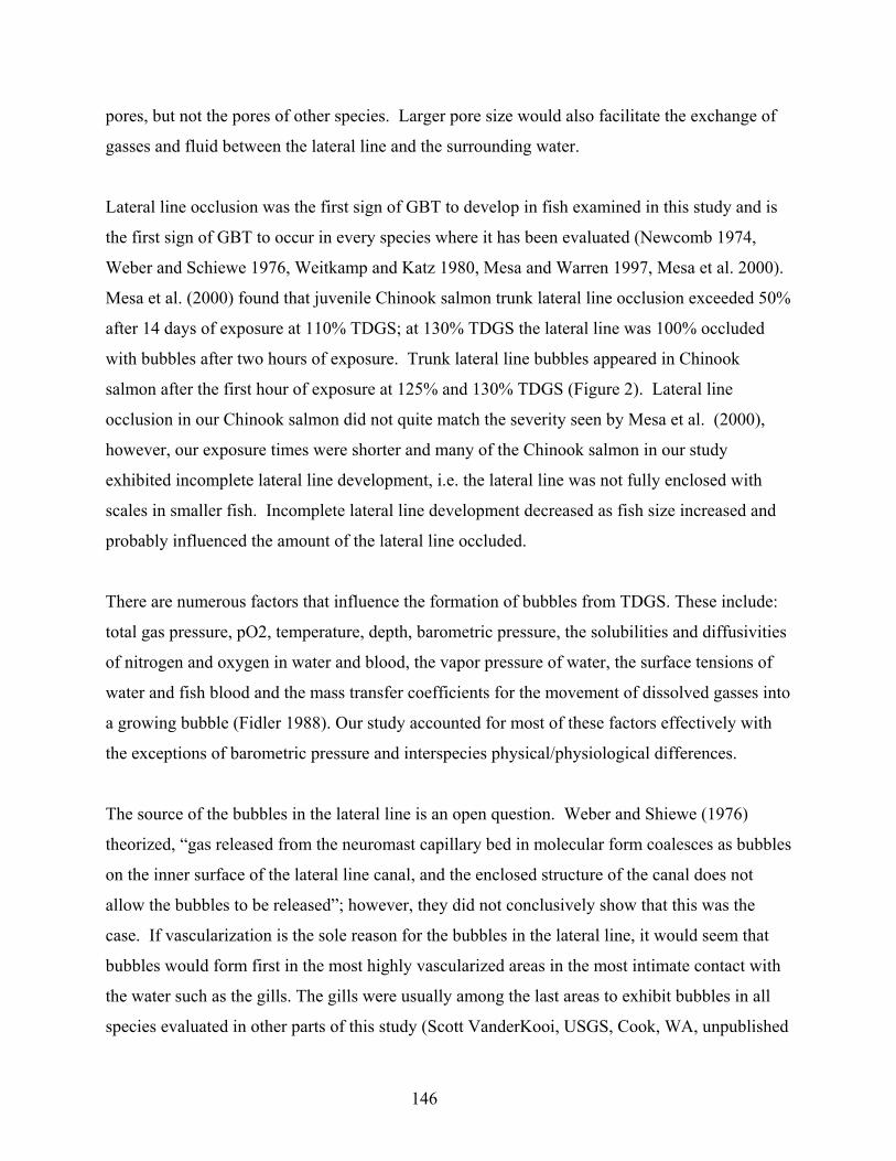
pores, but not the pores of other species. Larger pore size would also facilitate the exchange of
gasses and fluid between the lateral line and the surrounding water.
Lateral line occlusion was the first sign of GBT to develop in fish examined in this study and is
the first sign of GBT to occur in every species where it has been evaluated (Newcomb 1974,
Weber and Schiewe 1976, Weitkamp and Katz 1980, Mesa and Warren 1997, Mesa et al. 2000).
Mesa et al. (2000) found that juvenile Chinook salmon trunk lateral line occlusion exceeded 50%
after 14 days of exposure at 110% TDGS; at 130% TDGS the lateral line was 100% occluded
with bubbles after two hours of exposure. Trunk lateral line bubbles appeared in Chinook
salmon after the first hour of exposure at 125% and 130% TDGS (Figure 2). Lateral line
occlusion in our Chinook salmon did not quite match the severity seen by Mesa et al. (2000),
however, our exposure times were shorter and many of the Chinook salmon in our study
exhibited incomplete lateral line development, i.e. the lateral line was not fully enclosed with
scales in smaller fish. Incomplete lateral line development decreased as fish size increased and
probably influenced the amount of the lateral line occluded.
There are numerous factors that influence the formation of bubbles from TDGS. These include:
total gas pressure, pO2, temperature, depth, barometric pressure, the solubilities and diffusivities
of nitrogen and oxygen in water and blood, the vapor pressure of water, the surface tensions of
water and fish blood and the mass transfer coefficients for the movement of dissolved gasses into
a growing bubble (Fidler 1988). Our study accounted for most of these factors effectively with
the exceptions of barometric pressure and interspecies physical/physiological differences.
The source of the bubbles in the lateral line is an open question. Weber and Shiewe (1976)
theorized, “gas released from the neuromast capillary bed in molecular form coalesces as bubbles
on the inner surface of the lateral line canal, and the enclosed structure of the canal does not
allow the bubbles to be released”; however, they did not conclusively show that this was the
case. If vascularization is the sole reason for the bubbles in the lateral line, it would seem that
bubbles would form first in the most highly vascularized areas in the most intimate contact with
the water such as the gills. The gills were usually among the last areas to exhibit bubbles in all
species evaluated in other parts of this study (Scott VanderKooi, USGS, Cook, WA, unpublished
146

data). There are also extensive vascular beds on the surface of the body (Graham 1997,
Lillywhite and Maderson 1988) and at the base of the fins yet the lateral line canal is the first
area to exhibit bubble development. McDonough and Hemmingsen (1985) concluded that fish
movements induced bubble formation in fins “perhaps via tribonucleation” following
decompression, however they did not evaluate lateral line occlusion. The dominant GBT signs
observed by Newcomb (1974) and Mesa et al. (2000) in juvenile salmonids exposed to 110 and
115% TDGS were lateral line bubbles.
Perhaps the bubbles in the lateral line are the result of the gas being trapped and concentrated in
the covered canal but the fact that lateral line bubbles formed after only one hour (Figure 2) of
exposure in Chinook salmon seems to indicate a more active lateral line role. The possibility
that the lateral line may play a role in cutaneous respiration and creating lateral line bubbles in
the process has apparently not been examined (Rombough and Ure 1991, Graham 1997, Sacca
and Burggren 1982) but may provide an explanation for the source of lateral line bubbles. The
simplest explanation of the differences in lateral line occlusion relative to the pore diameter may
be that larger pore diameters allow more bubbles to escape, reducing lateral line occlusion.
However, this does not address the question of why the bubbles appear in the lateral line before
other GBT signs, apparently regardless of species.
In conclusion, differences in lateral line pore sizes between species were inversely related to
lateral line bubble occlusion in GBT experiments, indicating this measure of the severity of GBT
should not be used to compare GBT results between species unless they have similar lateral line
pore sizes. The uniformity of pore size within a species, irrespective of fish length, indicates that
intraspecific comparisons of lateral line occlusion are not affected by lateral line pore size. The
uniformity of the lateral line pores within a species also indicates that these pores may serve an
important, as yet unidentified function in fish.
Acknowledgements
We thank the staff at the Boise and Grand Coulee Dam offices of the U.S. Bureau of
Reclamation, the Confederated Tribes of the Colville Reservation, and the Columbia River Fish
147

Farm for their cooperation during this study. The work during this project was completed with
the help of David Venditti, Barbara Adams, Rhonda Dasher and Ross Huffman, which was
greatly appreciated. Thanks are also due to Dena Gadomski for her insightful comments. The
U.S. Geological Survey and the U.S. Bureau of Reclamation jointly funded this study.
148

References
Bleckmann, H. 1986. Role of the lateral line in fish behavior. Pages 177-202 in T. J. Pitcher, editor. The Behavior of Teleost Fishes. Johns Hopkins University Press, Baltimore, Maryland.
Bleckmann, H., Tittel, G., Blübaum, E. 1986. The lateral line system of surface-feeding:
anatomy, physiology, and behavior. Pages 501-526 in T. J. Pitcher, editor. The Behavior of Teleost Fishes. Johns Hopkins University Press, Baltimore, Maryland.
Bouck, G. R. 1980. Etiology of gas bubble disease. Transactions of the American Fisheries
Society 109:703-707. Coombs, S., Montgomery, J. C. 1999. The enigmatic lateral line system. Pages 319-362 in A.
N. Popper and R. R. Fay, editors. Comparative Hearing: Fishes and Amphibians. Springer-Verlag, New York, , New York.
Coombs, S., Janssen, J., Webb, J. F. 1988. Diversity of lateral line systems: evolutionary and
functional considerations. Pages 553-593 in J. Atema, R. R. Fay, A. N. Popper, and W. N. Tavolga, editors. Sensory Biology of Aquatic Animals. Springer-Verlag, New York, New York.
Counihan, T. D., Miller, A. I., Mesa, M. G., Parsely, M. J. 1998. The effects of dissolved gas
supersaturation on white sturgeon larvae. Transactions of the American Fisheries Society 127:316-322.
Dawley, E. M., Ebel, W. J. 1975. Effects of various concentrations of dissolved atmospheric
gas on juvenile Chinook salmon and steelhead trout. Fisheries Bulletin 73(4):787-796. Dijkgraaf, Sven, 1967. Biological significance of the lateral line organs. Pages 83-95 in P. H.
Cahn, editor. Lateral Line Detectors. Proceedings of a conference held at Yeshiva University, New York, April 16-18, 1966. Indiana University Press, Bloomington, New York.
Disler, N. N. 1960. Lateral line sense organs and their importance in fish behavior. Israel
Program for Scientific Translations, Academy of Sciences of the USSR, Severtsof Institute of Animal Morphology.
Ebel, W. J. 1971. Dissolved nitrogen concentrations in the Columbia and Snake Rivers in 1970
and their effects on Chinook salmon and steelhead trout. NOAA Technical Report NMFS SSRF-646.
Ebel, W. J., Raymond, H. L., Monan, G. E., Farr, W. E., Tanonaka, G. 1975. Effect of
atmospheric gas supersaturation caused by dams on salmon and steelhead trout of the Snake and Columbia rivers. NOAA. NMFS, NWFC, Seattle, WA.
149

Fickeisen, D. H., Montgomery, J. C. 1978. Tolerances of fishes to dissolved gas supersaturation
in deep tank bioassays. Transactions of the American Fisheries Society 107(2):376-381. Fidler, L.E. 1988. Gas bubble trauma in fish. Masters Thesis, pp. 16-17. Univ. of British
Columbia, Vancouver, B.C. Flock, A. 1967. Ultrastructure and function in the lateral line organs. Pages 83-95 in P. H.
Cahn, editor. Lateral Line Detectors. Proceedings of a conference held at Yeshiva University, New York, April 16-18, 1966. Indiana University Press, Bloomington, New York.
Gadomski, D. M., D. A. Venditti, T. C. Robinson, J. W. Beeman, and A. G. Maule. in press.
Distribution and relative abundance of fishes in littoral areas of Chief Joseph Reservoir, Columbia River. Northwest Science 78(1).
Graham, J. B. 1997. Air-breathing in fishes: evolution, diversity, and adaptation. Academic
Press Ltd., San Diego, California. Hans, K. M., Mesa, M. G., Maule, A. G. 1999. Rate of disappearance of gas bubble trauma
signs in juvenile salmonids. Journal of Aquatic Animal Health 11:383-390. Jakubowski, M. 1966. Cutaneous sense organs of fishes. Part VI. The lateral-line organs in the
perch-pike (Lucioperca lucioperca L), perch (Perca fluviatilis L.), their topography, innervation, vascularization, and structure. Acta Biologica Craco Series Zoology 9, 137-149.
Jakubowski, M. 1966 (A). Cutaneous sense organs of fishes. Part VI. Canal system of lateral-
line organs in Mullus barbatus ponticus Essipov and Spicara smaris L. (topography, innervation, structure). Acta Biologica Craco Series Zoology 9, 225-237.
Jakubowski, M. 1967. Cutaneous sense organs of fishes. Part VII. The structure of the system
of lateral-line organs in Percidae. Acta Biologica Craco Series Zoology 10, 69-81. Jakubowski, M. 1974. The structure of the lateral-line canal system and related bones in the
berycoid fish Hoplostethus mediterraneus Cuv. Et Val. (Trachichthydae, Pisces). Acta Anatomy 87, 261-274.
Janssen, J., Sideleva, V., Biga H. 1999. Use of the lateral line for feeding in two Lake Baikal
sculpins. Journal of Fish Biology 54:404-416. Krise, W. F., Herman, R. L. 1991. Resistance of underyearling and yearling Atlantic salmon
and lake trout to supersaturation with air. Journal of Aquatic Animal Health 3:248-253. Lillywhite, H. B., Maderson, P. F. A. 1988. The structure and permeability of integument.
American Zoology 28:945-962.
150

Lowenstein, O. 1957. The sense organs: the acoustico-lateralis system. Pages 155-158 in M. E.
Brown, editor. The Physiology of Fishes. Academic Press Inc., New York. Marsh, M. C., Gorham, F. P. 1905. The gas disease in fishes. Report of the United States
Bureau of Fisheries for 1904. Marshall, N. B. 1979. Developments in deep sea biology. Blandford Press Ltd., Poole, Dorset,
United Kingdom. Maruska, K. P. 2001. Morphology of the mechanosensory lateral line system in elasmobranch
fishes: ecological and behavioral considerations. Environmental Biology of Fishes 60:47-75.
McDonough, P. M., Hemmingsen, E. A. 1985. Swimming movements initiate bubble formation
in fish decompressed from elevated gas pressures. Comparative Biochemistry and Physiology 81A(1):209-212.
Mesa, M. G., Warren, J. J. 1997. Predator avoidance ability of juvenile Chinook salmon
(Onchorhynchus tshawytscha) subjected to sublethal exposures of gas-supersaturated water. Canadian Journal of Fisheries and Aquatic Sciences 54(4):757-764.
Mesa, M. G., Weiland, L. K., Maule, A. G. 2000. Progression and severity of gas bubble trauma
in juvenile salmonids. Transactions of the American Fisheries Society 129:174-185. Montgomery, J. C., Becker, C. D. 1980. Gas bubble disease in smallmouth bass and northern
pikeminnow from the Snake and Columbia rivers. Transactions of the American Fisheries Society 109:734-736.
Montgomery, J., Coombs, S., Janssen, J. 1994. Form and function relationships in lateral line
systems: comparative data from six species of Antarctic Notothenioid fish. Brain, Behavior and Evolution 44, 299-306.
Nebeker, A. V., Hauck, A. K., Baker, F. D., Weitz, S. L. 1980. Comparative responses of
speckled dace and cutthroat trout to air-supersaturated water. Transactions of the American Fisheries Society 109:760-764.
Newcomb, T. W. 1975. Changes in the blood chemistry of juvenile steelhead trout, Salmo
gairdneri, following sublethal exposure to nitrogen saturation. Proceedings of the Gas Bubble Disease Workshop, Battelle Pacific Northwest Laboratories, Richland, Washington.
Parker, G. H. 1904. The function of the lateral line organ in fishes. Bulletin of the US Bureau of
Fisheries. 24:185-207.
151

Rombough, P. J., Ure, D. 1991. Partitioning of oxygen uptake between cutaneous and branchial surfaces in larval and young juvenile Chinook salmon Oncorhynchus tshawytscha. Physiological and Biochemical Zoology 64(3), 717-727.
Ryan, B. A., Dawley, E. M., Nelson, R. A. 2000. Modeling the effects of supersaturated
dissolved gas on resident aquatic biota in the main-stem Snake and Columbia rivers. North American Journal of Fisheries Management 20:180-192.
Sacca, R., Burggren, W. 1982. Oxygen uptake in air and water in the air-breathing redfish
Calamoicthys calabaricus: Role of skin, gills and lungs. Journal of Experimental Biology 97:179-186.
Stroud, R. K., Bouck, G. R., Nebeker, A. V. 1975. Pathology of acute and chronic exposure of
salmonid fishes to supersaturated water in Chemistry and Physics of Aqueous Gas Solutions. The Electrochemical Society, Inc. pp. 435-449.
US Army Corps of Engineers, 2000. 1999. Total Dissolved Gas Monitoring Columbia and
Snake Rivers. Northwestern Division, Water Management Division, Reservoir Control Center, Water Quality Section.
Venditti, D. A., Robinson, T. C., Beeman, J. W., Adams, B. J., Maule, A. G. 2001. Gas bubble
disease in resident fish below Grand Coulee Dam. 1999 Annual Report of Research. Report to the U. S. Bureau of Reclamation by the U. S. Geological Survey.
Webb, J. F. 1989. Developmental constraints and evolution of the lateral line system in teleost
fishes. Pages 79-97 in S. Coombs, P. Görner, and H. Münz, editors. The mechanosensory lateral line: neurobiology and evolution. Springer-Verlag, New York, New York
Weber, D. D., Schiewe, M. H. 1976. Morphology and function of the lateral line of juvenile
steelhead trout in relation to gas-bubble disease. Journal of Fish Biology 9:217-233. Weitkamp, D. E., Katz, M. 1980. A review of dissolved gas supersaturation literature.
Transactions of the American Fisheries Society 109:659-702.
152

Table 1.— Mean (±SE) total dissolved gas supersaturation (TDGS) levels from lateral line occlusion studies in largescale sucker (LSS), longnose sucker (LNS), northern pikeminnow (NPM), redside shiner (RSS) and Chinook salmon (CHI). We measured TDGS in all treatment tanks (N = 4) at the start and end of all but two experiments. Value listed without SE is the TDGS measurement from a single treatment tank.
Species TDGS Starting TDGS (%) Ending TDGS (%)
Water temperature
(ºC) LSS 115% 115.5 ± 0.3 114.1 ± 0.1 12.2 ± 0.1
125% 124.6 ± 0.1 124.2 ± 0.2 12.2 ± 0.1
LNS 115% 114.6 ± 0.1 115.2 ± 0.1 12.4 ± 0.1
125% 125.8 ± 0.5 124.4 ± 0.3 12.1 ± 0.1
130% 130.2 ± 0.3 128.5 ± 0.2 12.4 ± 0.1
NPM 115% 114.8 ± 0.2 114.9 ± 0.1 12.2 ± 0.1
125% 124.9 ± 0.1 125.9 ± 0.2 12.2 ± 0.1
RSS 115% 115.7 ± 0.2 118.1 ± 0.2 11.9 ± 0.1
125% 126.3 ± 0.1 123.9 11.9 ± 0.1
130% 131.0 ± 0.1 130.3 ± 0.5 12.1 ± 0.1
CHI 125% 125.05 ± 0.1 124.7 ± 0.2 11.3 ± 0.1
130% 131.45 ± 0.1 130.6 ± 0.8 12.0 ± 0.1
153

Table 2. Pore diameter comparisons at different locations on the trunk lateral line of largescale sucker (LSS), longnose sucker (LNS), northern pikeminnow (NPM), redside shiner (RSS), and Chinook salmon (CHI). For explanation of pore measurement locations, see text. Diameters with the same letter do not differ significantly (P > 0.05).
Species Head pore diameter
(mm)
Mid - pore diameter
(mm)
Caudal pore diameter
(mm) Model statistics
LSS 0.19 (A) 0.17 (A) 0.17 (A) N = 180, F = 1.6, P= 0.2
LNS 0.58 (A) 0.51 (A:B) 0.43 (B) N = 63, F = 3.8, P= 0.02
NPM 0.082 (A) 0.083 (A) 0.086 (A) N = 195, F = 0.6, P= 0.5
RSS 0.056 (A) 0.053 (A) 0.057 (A) N = 81, F = 0.2, P= 0.8
CHI 0.12 (A) 0.12 (A) 0.14 (A) N = 105, F = 0.8, P= 0.5
154
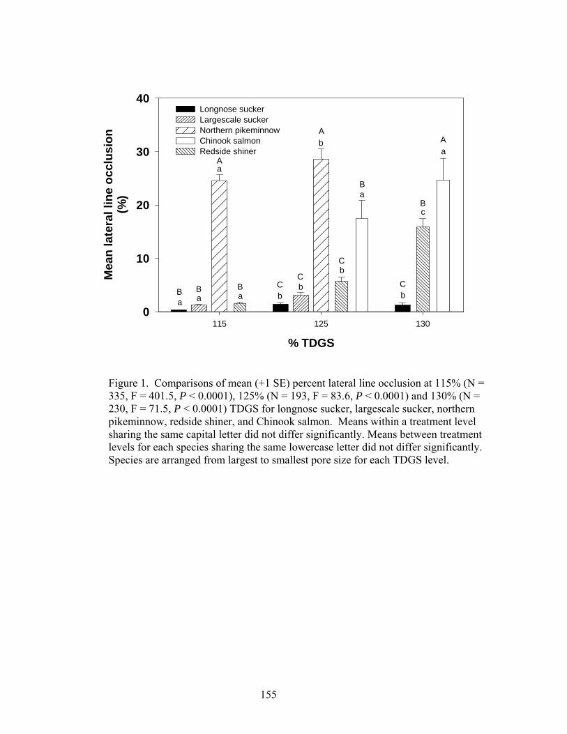
% TDGS115 125 130
Mea
n la
tera
l lin
e oc
clus
ion
(%)
0
10
20
30
40Longnose suckerLargescale suckerNorthern pikeminnowChinook salmonRedside shiner
A
B B B
A
B
CC
C
A
B
C
ab ba
b
a
b
a
b
c
a
a
Figure 1. Comparisons of mean (+1 SE) percent lateral line occlusion at 115% (N = 335, F = 401.5, P < 0.0001), 125% (N = 193, F = 83.6, P < 0.0001) and 130% (N = 230, F = 71.5, P < 0.0001) TDGS for longnose sucker, largescale sucker, northern pikeminnow, redside shiner, and Chinook salmon. Means within a treatment level sharing the same capital letter did not differ significantly. Means between treatment levels for each species sharing the same lowercase letter did not differ significantly. Species are arranged from largest to smallest pore size for each TDGS level.
155

a)
b)
0 100 200 300 400 500 600
Pore
dia
met
er(m
m)
0.0
0.2
0.4
0.6
0.8
1.0
N P MLS SLN S
Fork length(m m )
20 40 60 80 100 120 140 160 180 200 220
Pore
dia
met
er(m
m)
0.03
0.04
0.05
0.06
0.07
0.08
0.09
0.10
0.11
C H IR SS
Figure 2. Upper plate: Comparison of mean pore widths to fork lengths for longnose sucker (LNS), largescale sucker (LSS), and northern pikeminnow (NPM), and lower plate: Chinook salmon (CHI), and redside shiner (RSS). Lines are first order regressions.
156

Figure 3. Progression of lateral line bubble development in Chinook salmon at 125% (open boxes) and 130% TDGS (filled circles). First order regressions for 125% and 130% TDGS are dashed and solid lines, respectively.
157

Species
Mea
n po
re d
iam
eter
(mm
)
0.0
0.1
0.2
0.3
0.4
0.5
0.6
LNS LSS NPM CHI RSS
A
B
C
C:D D
Figure 4. Comparisons of mean (+ 1 SE) lateral line pore widths for longnose sucker (LNS), largescale sucker (LSS) northern pikeminnow (NPM), redside shiner (RSS), and Chinook salmon (CHI) (N = 256, F = 452, P < 0.0001). Means sharing the same letter did not differ significantly
158

Pore diameter(mm)
0.0 0.1 0.2 0.3 0.4 0.5 0.6 0.7 0.8
Late
ral l
ine
occl
usio
n(%
)
0
10
20
30
40
50
Y = 1.29*(X)/(3.16 + X)r2 = 0.17
Figure 5. Comparisons of mean percent lateral line occlusion for longnose sucker, largescale sucker, northern pikeminnow, redside shiner, and Chinook salmon and mean lateral line pore width.
159


