
Gene Ontology Annotation as Text Categorization: An Empirical Study
Kazuhiro Seki †,1
Organization of Advanced Science and Technology, Kobe University1-1 Rokkodai, Nada, Kobe 657-8501, JapanE-mail: [email protected]: +81-78-803-6480Fax: +81-78-803-6316
Javed Mostafa‡
‡ Laboratory of Applied Informatics Research, University of North Carolina at Chapel Hill216 Lenoir Drive, CB#3360, 100 Manning Hall, Chapel Hill, NC 27599-3360, USAE-mail: [email protected]: +1-919-962-2182
Kazuhiro Seki is the corresponding author.
1This work started when the first author was a Ph.D. student at Indiana University, Bloomington and has been continued at his current
institution.

2
Abstract
Gene Ontology (GO) consists of three structured controlled vocabularies, i.e., GO domains, developed for describ-
ing attributes of gene products, and its annotation is crucial to provide a common gateway to access different model
organism databases. This paper explores an effective application of text categorization methods to this highly prac-
tical problem in biology. As a first step, we attempt to tackle the automatic GO annotation task posed in the Text
Retrieval Conference (TREC) 2004 Genomics Track. Given a pair of genes and an article reference where the genes
appear, the task simulates assigning GO domain codes. We approach the problem with careful consideration of the
specialized terminology and pay special attention to various forms of gene synonyms, so as to exhaustively locate
the occurrences of the target gene. We extract the words around the spotted gene occurrences and used them to
represent the gene for GO domain code annotation. We regard the task as a text categorization problem and adopt
a variant of kNN with supervised term weighting schemes, making our method among the top-performing systems
in the TREC official evaluation. Furthermore, we investigate different feature selection policies in conjunction with
the treatment of terms associated with negative instances. Our experiments reveal that round-robin feature space
allocation with eliminating negative terms substantially improves performance as GO terms become specific.
KeywordsText Categorization, Gene Ontology Annotation, Supervised Term Weighting, Feature Selection Policy, Automatic
Database Curation, Genomic Information Retrieval

3
Molecular
function (MF)
Biological
process (BP)
Binding Motor
activity
N CellN Develop-
ment
BehaviorN N
GO
Cellular com-
ponent (CC)
Figure 1. Structure of Gene Ontology.
1 Introduction
Given the intense interest and the fast growing literature, biomedicine is an attractive domain for exploration of intel-
ligent information processing techniques, such as information retrieval (IR), information extraction, and information
visualization. Hence, it has been increasingly drawing much attention of researchers in IR and other related research
communities (Azuaje & Dopazo, 2005; Hirschman et al., 2002; Shatkay & Feldman, 2003), which in part resulted
in a track at Text Retrieval Conference (TREC)1 solely dedicated to the biomedical domain, namely, the Genomics
Track (Hersh, 2002, 2004; Hersh & Bhuptiraju, 2003; Hersh et al., 2004, 2005). This work is motivated by one of
the task challenges at the track and introduces a successful application of general text categorization and IR methods
to this evolving field of research targeting biomedical text.
In the post-genomic era, one of the major activities in molecular biology is to determine the precise functions
of individual genes or gene products, which has been producing a large number of publications with the help of
high throughput gene analyses. To structure the information related to gene functions scattered over the literature, a
great deal of efforts have been made to annotate articles by using the Gene Ontology2 (GO) terms. GO (The Gene
Ontology Consortium, 2000) was first developed as a collaborative project among three model organism databases,
FlyBase, the Saccharomyces Genome Database, and the Mouse Genome Database, in order to facilitate uniform
queries across the different databases. GO consists of three structured controlled vocabularies (ontologies) that
describe gene products in terms of their associated biological process (BP), cellular component (CC), and molecular
function (MF). The ontologies are structured—under the top three nodes—as directed acyclic graphs, which allow a
child term to have multiple parents. Figure 1 illustrates the structure of GO.
Because of the large number of publications and specialized content, GO annotation requires extensive human
efforts and substantial domain knowledge, usually conducted by experts. However, Baumgartner et al. (2007) re-
ported that current manual curation for GO annotation would never complete at the current rate of production through
careful analyses based on a metric known as the found/fixed graph from software engineering. Thus, there is a po-
1http://trec.nist.gov/2http://www.geneontology.org/

4
tential need to automate or semi-automate GO annotation, which could greatly alleviate the human curation. This
was one of the primary objectives pursued at the Genomics Track 2004 (Hersh et al., 2004).
The Genomics Track consisted of two tasks: ad hoc retrieval and categorization tasks. For the former, given
50 topics obtained through interviews with real research scientists, the participants were required to find relevant
documents from 10 years’ worth of MEDLINE data. The latter task, which is our focus in this paper, was composed
of two sub-tasks; one was called the triage task and the other the annotation task. Both tasks mimicked some parts
of the GO annotation process currently carried out by human experts at Mouse Genome Informatics (MGI) initiative.
In brief, the goal of the triage task was to correctly identify whether an input article contains experimental evidence
that warrants GO annotation regardless of particular GO terms. The annotation task was the next step to the triage
decision, and the primary goal was to correctly assign GO domain codes, i.e., MF, BP, and CC (not the actual GO
terms) or not to assign them, i.e., negative, for each of the given genes that appear in the article.3 Note that there
may be more than one gene associated with an article and there may be more than one domain code assigned to a
gene. The secondary goal of the annotation task—although not discussed in this paper—was to identify the correct
GO evidence code that indicates the type of evidence for the assigned domain code. Compared to the other tasks
which attracted numbers of runs and participants, the latter part of the annotation task was challenged by only two
research groups including ours (Seki et al., 2004), which partly indicates the difficulty of the task.
The triage task can be seen as a standard text categorization problem to classify an input article into one of the
predefined categories (positive and negative), while the annotation task requires to classify not an article as a whole
but each given gene appearing in the article. In other words, each 〈article, gene〉 pair is to be independently treated
and classified even when two (or more) genes appear in a single article. We address the problem by extracting
document fragments that are likely to contain the gene in question by gene name expansion and a flexible term
matching scheme. The resulting document fragments are then used for representing the particular gene. For classifi-
cation, we use a variant of k-Nearest Neighbor (kNN) classifiers with a supervised term weighting scheme (Debole
& Sebastiani, 2003) which consider word distributions in different categories.
This paper focuses on an application of general text categorization and IR techniques to the domain-specific
problem requiring the involvement of an expert and it typically is a highly intellectual process demanding a care-
ful consideration of the properties of the terminology in biomedicine. In the following, Section 2 introduces our
proposed framework for GO domain code annotation in detail, and then Section 3 describes the data and evalua-
tion measures used for our experiments. In Section 4, we show the validity of our framework through a number
of experiments with various different settings. In addition, we compare different feature selection policies to study
their effects on GO annotation. Section 5 reports an application of our framework to the triage task as well. After
Section 6 discussing the related work, Section 7 concludes this paper with a brief summary of our approach and
major findings, and possible future directions.
3Assuming perfect triage decision, there would not be negative cases at the annotation stage. However, there were negative instances
purposefully included in the TREC data (see Section 3.2).

5
2 Methods
This section details our proposed framework for automatic GO domain code annotation. Hereafter, we will refer to
GO domain code annotation as “GO annotation” for short unless otherwise noted. First, Section 2.1 describes how
input is processed and represented in a vector space, and then Section 2.2 presents a classifier to be used for GO
annotation.
2.1 Document representation
2.1.1 Identification of relevant paragraphs
GO annotation needs to be made not for each input article but for each gene for which there is experimental evidence
that warrants GO annotation. Therefore, each 〈article, gene〉 pair can be treated as a “document” or “text” in the
sense of text categorization. For this purpose, we propose a simple but effective approach to extract only the text
fragments that are likely to contain the gene in question and treat a set of the extracted text fragments as a “document”
to represent the 〈article, gene〉 pair. This process can be broken down into gene name expansion and gene name
identification, each explained in the following.
Gene name expansion Gene name expansion refers to a process to associate synonyms with a given gene name.
Gene names (and their products) are known to have several types of synonyms including aliases, abbreviations, and
gene symbols (Sehgal & Srinivasan, 2006). For instance, “membrane associated transporter protein” (GeneID4:
22293) can be referred to as underwhite, dominant brown, Matp, uw, Dbr, bls, Aim1, etc. Therefore, all of these
names should be considered to identify text fragments mentioning the gene. To obtain such synonyms, we used
two sources of information: the article itself and a gene name dictionary. As described later in Section 3, the input
article is annotated with SGML tags and there are two relevant fields, <KEYWORD> and <GLOSSARY>, in which a gene
name and its synonym may be explicitly stated.5 An example is given in Figure 2, where five pairs of entity names
and their abbreviations are defined. If the given gene is found in the pairs, we use the information to expand the
gene name. Incidentally, we also examined the use of body text because gene name abbreviations often appear with
parentheses immediately following the official names (Schwartz & Hearst, 2003). However, it slightly degraded
classification in our preliminary experiments and thus was not used thereafter.
As another source of gene name expansion, a gene name dictionary was automatically compiled from existing
databases. For this work, we experimentally used the SWISS-PROT (O’Donovan et al., 2002) and LocusLink (Pruitt
& Maglott, 2001) databases.6 The resulting name dictionary contains 493,473 records, where each record has a
4From the Entrez Gene database available at http://www.ncbi.nlm.nih.gov/sites/entrez?db=gene5The DTD is found at http://highwire.stanford.edu/about/dtd/6LocusLink has been superseded by Entrez Gene.

6
<GLOSSARY>
<DEFLIST>
<TERM ID="G1">MHC</TERM>
<DD><P>major histocompatibility complex</P></DD>
<TERM ID="G2">Hsp</TERM>
<DD><P>heat shock protein</P></DD>
<TERM ID="G3">T4Hsp10</TERM>
<DD><P>bacteriophage T4 Hsp10</P></DD>
<TERM ID="G4">MES</TERM>
<DD><P>4-morpholineethanesulfonic acid</P></DD>
<TERM ID="G5">E-64</TERM>
<DD><P>trans-epoxysuccinyl-<SC>l</SC>-leucylamido-(4-guanidino)butane</P></DD>
</DEFLIST>
</GLOSSARY>
Figure 2. An excerpt of a <GLOSSARY> field from an SGML file (bc0102000155.gml in the TREC 2004 Genomics Track
data set for GO annotation task; see Section 3.2 for detail).
gene/protein name as an index and lists its synonyms. Hereafter, we use the word “gene names” to refer to all of
official names, aliases, abbreviations, and gene symbols.
It is often the case that gene name dictionaries automatically compiled from existing databases, such as ours,
are noisy due to multi-sense gene names, inconsistent format in the databases, etc. Therefore, it usually requires
manual curation to build a high-quality dictionary (Egorov et al., 2004; Hanisch et al., 2003), which is important for
general-purpose gene name recognition systems. Fortunately, the quality of a dictionary would not be as important
in our application, because even if the dictionary provides wrong gene names as synonyms of a given gene, those
wrong names are unlikely to appear in an article as they are irrelevant to the given target gene with which the article
is associated.
Gene name identification The next step is to find text fragments mentioning the gene in question, where we
considered a paragraph as a unit of analysis. Here, the problem is that, besides synonyms, gene names often have
many variants due to arbitrary use of special symbols, white space, and capital and small letters (Cohen et al., 2002;
Cohen, 2005; Fang et al., 2006; Morgan et al., 2007). To tolerate these minor differences in identifying gene names,
both gene names and text were normalized using the following heuristic rules partly derived from the work by Cohen
et al. (2002). Note that the actual order of applying the rules does not make difference.
• Replace all special symbols (non-alphanumeric characters) with space (e.g., NF-kappa→ NF kappa)

7
• Insert space between different character types, such as alphabets and numerals (e.g., Diet1→ Diet 1)
• Insert space between Greek alphabets and other words (e.g., kappaB→ kappa B)
• Lowercase all characters
Then, each paragraph (identified by SGML tags) in the article was scanned if it contained any of the gene names
associated with the gene in question. Note that section titles were appended to each paragraph since they are often
descriptive. In addition, if the paragraph referred to figures and/or tables for the first time in the article, their captions
were also appended to the paragraph.
We have so far obtained gene name synonyms and normalized both gene names and text to facilitate gene name
identification. However, there remains another problem. That is, gene names are frequently written in slightly
different forms with extra words, different word order, etc. For example, “peroxisome proliferator activated receptor
binding protein” (GeneID: 19014) may be referred to as “peroxisome proliferator activator receptor (PPAR)-binding
protein” where underlines indicate the differences. To deal with the problem, we used approximate word matching.
To be precise, for each target gene name (denoted as gene) and each candidate which mentions any word composing
the gene name (denoted as candidate), a word-overlap score defined below was computed.
Overlap(gene, candidate) =M − α · U
N + β(1)
where M and U represent the number of matching and unmatching words, respectively; α is a penalty for unmatching
words (set to 0.3); N is the number of words composing the gene name; and β penalizes shorter gene names (set to 2).
If any candidate associated with a paragraph had a score exceeding a predefined threshold (set to 0.3), the paragraph
was used to represent the 〈article, gene〉 pair after stopword removal and stemming by the PubMed stopword list7 and
Lovins stemmer (Lovins, 1968), respectively. For instance, the example of “peroxisome. . .” above has five matching
and two unmatching words, resulting in an overlap score of 0.55. Because it is greater than the threshold (0.3), the
paragraph containing the candidate is extracted and used in part to represent the corresponding 〈article, gene〉 pair.
Incidentally, the values of the parameters were arbitrarily determined based on our preliminary experiments using
the training data (see Section 3 for the description of the data set).
Here, we treated a paragraph as a unit of extraction since it is thought to be organized in a single topic and seems
to be an appropriate unit. In Section 4.2, we will examine other alternatives.
2.1.2 MeSH terms
Along with the article itself, we took advantage of external resources, specifically, Medical Subject Heading
(MeSH)8 terms assigned to the article. MeSH is a controlled vocabulary developed at the National Library of
Medicine (NLM) for indexing biomedical articles and is annotated by human experts at NLM.
7http://www.ncbi.nlm.nih.gov/entrez/query/static/ help/pmhelp.html8http://www.nlm.nih.gov/mesh/

8
For each input article, all the associated MeSH terms were obtained from the MEDLINE database9 using Entrez
Utilities.10 Because these MeSH terms are annotated with the article (not with particular genes in it), they were
added to every document (i.e., a set of paragraphs) representing a pair of the article and any gene coupled with it.
Note that a special symbol MESH+ was concatenated to each MeSH term so as to distinguish MeSH from other terms.
2.1.3 Feature selection
Feature selection identifies the features (terms) that are more informative in terms of classification according to
some statistic measure, which not only reduces the size of the feature space but often improves classification (Yang
& Pedersen, 1997). For this work, we adopted the chi-square statistic and compute it for every term composing the
“documents” obtained through the previous steps.
Chi-square statistic of term t in class c is defined as:
χ2(t, c) =N(AD −CB)2
(A + C) (B + D) (A + B) (C + D)(2)
where c is one of the GO domain codes (BP, MF, and CC) or negative (NEG), A is the number of documents
containing term t in class c, B is the number of documents containing t that are not in c, C is the number of
documents not containing t in c, D is the number of documents not containing t in classes that are not in c, and
N is the total number of documents. For each term t, chi-square statistic was computed for every class, and the
maximum score was taken as the chi-square statistic for term t; that is, χ2(t) = maxi χ2(t, ci). Only the top n terms
with higher chi-square were selected and used for the following processes. We empirically chose n=3000 based on
our preliminary experiments. It should be mentioned that, for real-world applications, a smaller feature set would
be preferred from the view point of computer resources and processing time. However, this work pursues highest
performance possibly obtained by the proposed framework, where those issues are secondary.
2.1.4 Term weighting
Each 〈article, gene〉 pair is associated with a set of selected terms in the preceding steps. To apply kNN for classifi-
cation as described in the next section, we convert it to a term vector using the classic vector space model (Salton &
McGill, 1983) with conventional TFIDF (term frequency-inverse document frequency) defined as:
TFIDF(t, d) = (1 + log TF(t, d)) · logN
DF(t)(3)
where TF(t, d) is a term frequency of term t within document d, N is the total number of documents, and DF(t) is
the number of documents in which term t appears. In cases where TF(t, d) = 0, TFIDF(t, d) is defined to be 0.
9http://www.ncbi.nlm.nih.gov/entrez/query.fcgi10http://www.ncbi.nlm.nih.gov/entrez/query/static/eutils help.html

9
We also examine another term weighting scheme, so called supervised term weighting, proposed by Debole &
Sebastiani (2003). It takes into account pre-labeled class information in training data and reuses statistic computed
in the feature selection step (e.g., chi-square statistics, information gain, etc.) in place of IDF. We use TFCHI which
is defined as a product of TF and chi-square statistic. Specifically, we test two variants of the scheme, denoted as
TFCHI1 and TFCHI2, respectively.
TFCHI1(t, d) = (1 + log TF(t, d)) · χ2(t)
TFCHI2(t, d) = (1 + log TF(t, d)) · log χ2(t)(4)
2.2 kNN classifiers
We use a variant of kNN classifiers to assign GO domain codes to each pair of article and gene. kNN is an instance-
based classifier and is reported as one of the best classifiers for text categorization in both newswire and medical
domains (Yang & Liu, 1999). In brief, it classifies input v to one or more predefined classes depending on what
classes its neighbors belong to. The decision rule can be expressed as
if Score(c, v) =∑
i
sim(v, nc,i) > tc, then assign c to v (5)
where nc is the k nearest neighbors having class c ∈ {BP, MF, CC}, tc is a per-class threshold, and sim(v, nc,i) returns
cosine similarity between the arguments. Threshold tc can be optimized to maximize an arbitrary metric (e.g., F1
score) using tuning data.
In cases where none of the GO domain codes is assigned to input v, then it is considered to be negative. This
ensures that an input does not have both positive (BP, MF, or CC) and negative classes together. It should be noted
that, however, negative class does affect classification because more negative instances included in k neighbors
generally lead to lower scores for the positive classes.
We slightly modified the standard scoring scheme above to multiply the similarity scores by the number of k
neighbors having class c, denoted as |nc|.
if Score(c, v) =∑
i
sim(v, nc,i) × |nc| > tc, then assign c to v (6)
It intended to boost the scores for more frequent classes within the k neighbors. This modification slightly but
constantly improved classification (around 2% in F1 score), presumably because for evaluation we used micro-
averaged F1 which emphasizes larger classes (see Section 3.3).

10
3 Experimental Setup
3.1 Implementation
We implemented for evaluation the categorization framework described in Section 2 in the R programming language,
where data preprocessing including feature selection was done by Perl scripts. All the experiments reported in this
paper were carried out on a PC running Linux with two 2.00 GHz Intel Pentium 4 processors and 3.5 GB of RAM.
3.2 Data sets
For evaluation, we use the data set from the Genomics Track 2004 GO annotation task (Cohen & Hersh, 2006).
The data set is composed of 504 full-text articles for training and 378 for test, both in SGML format. Each of the
articles is associated with one or more genes and each gene is annotated with one or more classes (BP, MF, and
CC) or negative by MGI curators. The total number of triplets 〈article, gene, class〉 is 1,661 (589 positives and 1,072
negatives) and 1,077 (495 positives and 582 negatives) for the training and test data, respectively. Because gene
names often contain Greek alphabets, character entities used for representing Greek alphabets (e.g., “&agr;” for α)
were converted to the corresponding English spellings (e.g., alpha) in advance to facilitate gene name identification.
The training data were used for tuning parameters including the number of k neighbors and per-class thresholds
tc in Equation (6) and were used as pre-labeled instances in classifying the test data by kNN.
3.3 Measures
Following the TREC Genomics Track, we used the micro-averaged F1 score as an evaluation metric for GO anno-
tation, so as to make our results directly comparable with the official evaluation. Micro-averaged F1 is an instance-
based measure paying equal importance to each instance (or label) and hence more influenced by the performance in
larger classes, whereas the another measure—macro-averaged F1—is class-based, paying equal importance to each
class (Jackson & Moulinier, 2007). Both types of F1 are defined as the harmonic mean of precision and recall, which
are calculated based on either instances or classes depending on the type of F1 intended. Equation (7) presents the
definitions of the micro-averaged measures, where classes are biological process (BP), cellular component (CC),
and molecular function (MF) and do not include negative (NEG).
Recall =# of class labels correctly predicted by the system
# of true class labels
Precision =# of class labels correctly predicted by the system
# of class labels predicted by the system
F1 =2 × Precision × Recall
Precision + Recall
(7)

11
Table 1: The TREC official results and our results for GO domain code annotation (on the test data set).
Prec Recall F1
Best 0.441 0.769 0.561
TREC Worst 0.169 0.133 0.149
Mean 0.360 0.581 0.382
TFIDF 0.445 0.849 0.584
Ours TFCHI1 0.460 0.764 0.575
TFCHI2 0.501 0.707 0.586
4 Results and discussion
4.1 Primary results
Our proposed framework for GO annotation was applied to the test data, where the per-class thresholds tc in Equa-
tion (6) and other parameters including the number of k neighbors were optimized to maximize F1 for each term
weighting scheme using the training data.11 Table 1 compares our results (TFIDF, TFCHI1, and TFCHI2) on the test
data and the representative results from the TREC official evaluation. For the annotation task, there were 36 runs
submitted from 10 different research groups (Hersh, 2004). Incidentally, the best result in TREC was also obtained
by our group using TFCHI2 (Seki et al., 2004; Seki & Mostafa, 2005). The improvement from 0.561 (“Best”) to
0.586 (“TFCHI2”) is due to a few corrections in our codes for feature selection and classification. It should be also
mentioned that the TFCHI2 scheme performed the best for the GO domain and evidence codes annotation task at the
TREC 2004 as well (see Hersh, 2004; Seki et al., 2004).
We can observe that, despite the simplicity of our approach, it performed quite well especially with TFIDF and
TFCHI2. In the following sections, we take a closer look at major features or components of our framework and
discuss their contribution.
4.2 Additional experiments
4.2.1 Alternative settings
We have made a number of design decisions in developing our framework and system features. To investigate the
impact of the decisions, we conducted several experiments with various different settings. Particularly, we were
interested whether the features or components below had made any impact on GO annotation.
• Gene name identification: We identified the paragraphs that were likely to contain the target gene using
approximate word matching (see Section 2.1). Did it actually improve GO annotation? To answer the question, we
11For instance, for TFCHI2, k was set to 60 and tc was set to 211.4, 194.4, and 275.8 for BP, CC, and MF, respectively.

12
used exact word matching to identify gene names.
• Gene name dictionary: Assuming gene name identification above worked, did the dictionary for gene name
expansion contribute to the performance? We examined our framework without the help of the dictionary.
• Glossary and keyword fields: Similarly, did the use of SGML tags, <GLOSSARY> and <KEYWORD>, for finding
gene name synonyms improve GO annotation? We tested our framework without the information.
• MeSH terms: Did the inclusion of MeSH terms contribute to classification? We tested our framework without
using MeSH terms.
• Unit of extraction: Was a paragraph as a unit of extraction appropriate? We explored other units:
• Only the sentence containing the target gene (denoted as G)
• In addition to G, an immediately succeeding sentence (denoted as G+S)
• In addition to G+S, an immediately preceding sentence (denoted as P+G+S)
• The entire article irrespective of the target gene (denoted as ART)
Note that, however, we did not let both G+S and P+G+S go beyond paragraph boundaries. Incidentally, our frame-
work focusing on paragraphs would be placed somewhere between P+G+S and ART.
4.2.2 Empirical observations
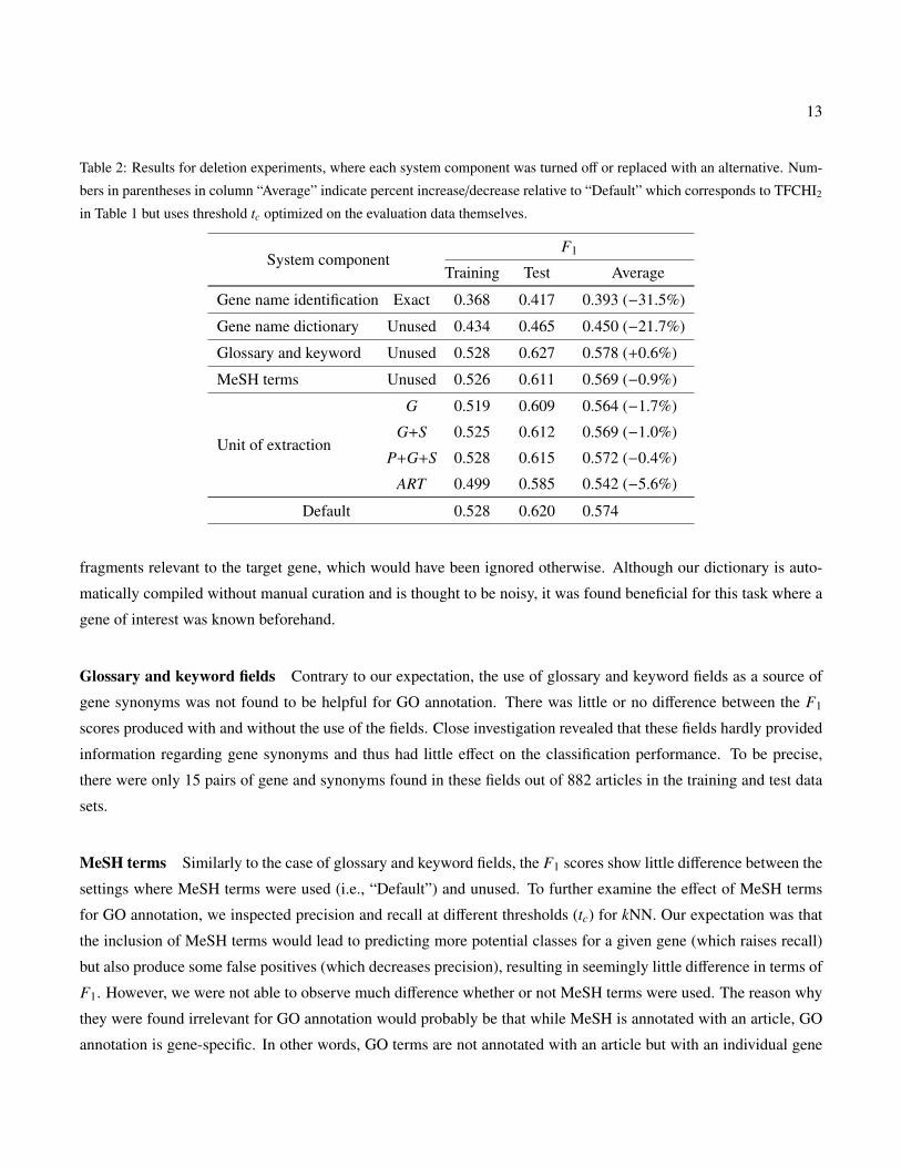
Table 2 summarizes the system performance in F1 for each of the experimental settings described above, where
the training data were classified using leave-one-out cross-validation, while the test data were classified using the
training data as before. Note that the bottom row “Default” corresponds to TFCHI2 in Table 1 but shows higher F1.
This is because threshold tc for kNN was optimized on the evaluation data themselves for this experiment in order
to compare possible maximum gain by different settings.
Gene name identification Using exact word matching for gene name identification severely deteriorated the per-
formance both on the training and test data sets. This supports our observation that gene names are often written
in slightly different forms from their canonical ones (i.e., database entries). Thus, a flexible name matching scheme
such as the one proposed here is needed in order to exhaustively locate gene name occurrences. A possible drawback
of approximate word matching is that it may recognize irrelevant word sequences as gene names (i.e., false posi-
tives), leading to an inclusion of irrelevant text fragments into the representation of the target gene. However, the
influence can be minimized by properly tuning the threshold (and parameters) for the word-overlap score defined in
Equation (1). Based on our experiments, a threshold of 0.3 (which was used for our experiments) constantly yielded
the best performance.
Gene name dictionary Disabling the gene name dictionary also decreased F1 score both on the training and
test data by 21.7% on average. It verifies that gene name expansion using the dictionary did help to identify text
13
Table 2: Results for deletion experiments, where each system component was turned off or replaced with an alternative. Num-
bers in parentheses in column “Average” indicate percent increase/decrease relative to “Default” which corresponds to TFCHI2
in Table 1 but uses threshold tc optimized on the evaluation data themselves.
System componentF1
Training Test Average
Gene name identification Exact 0.368 0.417 0.393 (−31.5%)
Gene name dictionary Unused 0.434 0.465 0.450 (−21.7%)
Glossary and keyword Unused 0.528 0.627 0.578 (+0.6%)
MeSH terms Unused 0.526 0.611 0.569 (−0.9%)
Unit of extraction
G 0.519 0.609 0.564 (−1.7%)
G+S 0.525 0.612 0.569 (−1.0%)
P+G+S 0.528 0.615 0.572 (−0.4%)
ART 0.499 0.585 0.542 (−5.6%)
Default 0.528 0.620 0.574
fragments relevant to the target gene, which would have been ignored otherwise. Although our dictionary is auto-
matically compiled without manual curation and is thought to be noisy, it was found beneficial for this task where a
gene of interest was known beforehand.
Glossary and keyword fields Contrary to our expectation, the use of glossary and keyword fields as a source of
gene synonyms was not found to be helpful for GO annotation. There was little or no difference between the F1
scores produced with and without the use of the fields. Close investigation revealed that these fields hardly provided
information regarding gene synonyms and thus had little effect on the classification performance. To be precise,
there were only 15 pairs of gene and synonyms found in these fields out of 882 articles in the training and test data
sets.
MeSH terms Similarly to the case of glossary and keyword fields, the F1 scores show little difference between the
settings where MeSH terms were used (i.e., “Default”) and unused. To further examine the effect of MeSH terms
for GO annotation, we inspected precision and recall at different thresholds (tc) for kNN. Our expectation was that
the inclusion of MeSH terms would lead to predicting more potential classes for a given gene (which raises recall)
but also produce some false positives (which decreases precision), resulting in seemingly little difference in terms of
F1. However, we were not able to observe much difference whether or not MeSH terms were used. The reason why
they were found irrelevant for GO annotation would probably be that while MeSH is annotated with an article, GO
annotation is gene-specific. In other words, GO terms are not annotated with an article but with an individual gene

14
0.2 0.4 0.6 0.8 1.0
0.2
0.3
0.4
0.5
0.6
0.7
0.8
Recall
Pre
cis
ion
Paragraphs (test)
Article (test)
Paragraphs (train)
Article (train)
Figure 3. Relation between recall and precision where either selected paragraphs (i.e., Default) or entire article (ART) were
used for document representation.
appearing in it. Therefore, it might be possible to improve GO annotation if each MeSH term could be precisely
associated with an individual gene.
Unit of extraction Four different units were compared in extracting text fragments. In short, as going from G
(only sentences containing the target gene) to ART (entire article) in Table 2, more text was extracted for document
representation. As can be seen, there is a trend that F1 gradually increases from G to P+G+S (sentence containing
the target gene plus immediately preceding and succeeding sentences) and then decreases when the entire article was
used (i.e., ART) compared to “Default.” From this observation, it is verified that our framework to extract paragraphs
is optimum, although the difference from G, G+S, or P+G+S is insignificant.
To highlight the effect of extracting gene-bearing paragraphs, Figure 3 compares recall-precision curves for
selected paragraphs (Default) and entire article (ART) on the training and test data.
The top two curves were obtained on the test data and the bottom two were obtained on the training. Overall, it can
be seen that using only paragraphs mentioning the target gene (shown as solid lines) improves precision at the same
recall level both on the training and test data. Especially, the effect is more evident with higher recall. This means
that selectively using only relevant paragraphs suppresses false positives when lowering the threshold.

15
Title Abs Intro Proc Method Result MeSH All
Sections
F1
0.0
0.1
0.2
0.3
0.4
0.5
0.6
73%
86%
78% 79%
53%
97%
79%
100%
Figure 4. Results produced by individual sections. “All” used all the sections. Percentages above bars indicate the respective
proportions to “All”.
4.2.3 Contributions of different parts of articles
Our current framework makes use of paragraph boundaries in extracting text fragments containing the target gene.
However, it does not consider or distinguish the structure of an article, e.g., sections. Such information may be useful
for GO annotation because different parts of articles may have different importance with respect to GO annotation.
For example, “Results” or “Conclusion” sections may be more relevant to GO annotation as they usually report
findings from experiments. Therefore, we examined how useful the individual sections were for GO annotation by
using only one section at a time from which gene-bearing paragraphs were extracted. Specifically, we focused on
the following sections: abstract, introduction, procedures, methods, and results. Both discussion and conclusion
sections were regarded as result sections since they are sometimes not clearly separated from results (e.g., “Results
and Discussion” section). Incidentally, these sections were identified based on section names annotated by SGML
tags.
Figure 4 shows a histogram for F1 scores produced using individual sections on the training data, where we
include results from the use of only titles and only MeSH terms for comparison. The rightmost bar “All” used all the
sections including MeSH, which corresponds to “Default” in Table 2.
Surprisingly, the Result section alone yielded almost as good F1 as All, followed by Abs (abstract), MeSH, Proc
(procedures), and so on. On the other hand, the Method sections showed the worst performance—worse than only
titles—for GO annotation. This is, however, consistent with the suggestion given by experts that “Materials and
Methods” sections can be used for identifying species and GO evidence codes but should not be used for predicting

16
Table 3: System performance in F1 for different feature selection policies.
Policy Term weight Training Test Average
max χ2TFIDF 0.512 0.619 0.566
TFCHI2 0.528 0.620 0.574
Round-robinTFIDF 0.510 0.621 0.566
TFCHI2 0.525 0.629 0.577
GO terms (Camon et al., 2005). Although not presented here, our experiments on the test data also showed similar
results.
In an attempt to improve GO annotation, we explored a better use of the logical structure of articles in two
ways: a) we weighted each section differently considering its relative importance, and b) we appended section
information to each term to indicate where the term came from. For example, the same word “cell” was treated as
two distinct features in cases where it was found in Title and Method sections, respectively, as “Title+cell” and
“Method+cell.” Unfortunately, both attempts failed to improve system performance and rather decreased F1 a few
points. More work is needed to identify the best use of article structure.
4.3 Discussions on alternative feature selection policies
4.3.1 Round-robin feature space allocation
As described in Section 2.1.3, we selected discriminative features (terms) based on the maximum chi-square statistic,
maxi χ2(t, ci). A potential shortcoming of this feature selection policy is that it by definition does not take into
account how many features took maximum chi-square for each class. As a result, the distribution of features is not
necessarily balanced. In fact, among the 3000 features selected for the preceding experiments, 242 took maximum
in class BP, 339 in MF, 463 in CC, and 1956 in NEG.
An alternative feature selection policy would be the round-robin proposed by Forman (2004), which allocates
the feature space equally among all classes. For instance, given four classes, 3000 features would be equally divided
into four (i.e., 750 features) and be allocated to each class. The intention of the policy is to avoid selecting a large
number of strong features for only some “easy” classes and to select a certain number of good predictive features
for every class including more difficult ones. On 19 different benchmark data sets, Forman demonstrated that the
round-robin policy could gain a substantial improvement over max χ2 especially when the feature size was small.
In order to examine if Forman’s observation holds for GO annotation, we tested the round-robin policy on our
data sets while using TFIDF and TFCHI2. Note that all the parameters remained the same as the best setting from the
previous experiments. Only exception was threshold tc for kNN as before, which was optimized on the evaluation
data themselves for cross-setting comparison. The results are summarized in Table 3.

17
GO
Cellular
component
Molecular
function
Biological
process
Biological
adhesion
Cellular
process
a a
1
N
d
1
Cell
adhesion
De
pth
leve
l
12
3
Figure 5. An illustration of different levels of specificity in GO hierarchy. Note that GO allows a node to have multiple parents.
In brief, the results are mixed; when adopting round-robin, F1 decreased on the training data and increased on
the test data. In either event, however, the difference is insignificant. The small effect may be due to the fact that the
number of classes dealt with in this task is very small. With only four classes (and the relatively large feature size
of 3000), it would be easy to include a reasonable number of features for each class without applying round-robin
even though the distribution is skewed. Also, because the number of classes is small, it is likely that good features
for one class are also good features for the others.
To investigate the impact of different feature selection policies on GO annotation with a larger number of classes,
we conducted another set of experiments by looking at more specific GO terms instead of the GO domains. The next
section describes the design of the experiments and reports the results.
4.3.2 GO term annotation
Each gene (or its product) appearing in the TREC Genomics Track data set is annotated with one or more GO
terms along with GO domains. For example, “vascular cell adhesion molecule 1” (GeneID: 22329) appearing in a
MEDLINE article (PubMed ID: 12021259) is assigned, in addition to a GO domain code BP, a more specific GO
term “cell adhesion (GO code: 0008378),” which is at the third depth level of the GO hierarchy as illustrated in
Figure 5. Based on these GO term annotations, we examined how the round-robin policy affected automatic GO
annotation for different levels of specificity. Incidentally, GO annotation at the deeper depth level is inherently more
difficult since there are combinatorially more classes (GO terms) barely used (Ogren et al., 2005), meaning less
training instances for many classes.
For each depth level from 1 (corresponding to GO domains) to 6, we carried out experiments to assign GO terms
at that level. Note that a greater depth level involves more classes (GO terms). Since the annotated GO terms in our
data set had different depth levels, we traced back each annotated GO term to the root of the ontology and re-assigned
GO term(s) at any given level in-between. For instance, suppose that we are attempting to annotate GO terms at the
second depth level. In this case, both “biological adhesion” and “cellular process” are treated as the correct GO

180.0
0.1
0.2
0.3
0.4
0.5
0.6
Depth level
F1
1 2 3 4 5 6
TFCHI2TFCHI2 w/ Round−Robin
TFIDF
TFIDF w/ Round−Robin
0 50 100 150 200
Number of classes (GO terms)
0.0
0.1
0.2
0.3
0.4
0.5
0.6
Depth level
F1
1 2 3 4 5 6
TFCHI2TFCHI2 w/ Round−Robin
TFIDF
TFIDF w/ Round−Robin
0 50 100 150 200
Number of classes (GO terms)
Figure 6. Relations between system performance in F1 and different depth levels of Gene Ontology. The left and right figures
show the results on training data and test data, respectively.
terms for “cell adhesion” because they are ancestors (parents) of “cell adhesion” at the second depth level. In cases
where the depth level is greater than that of the original GO term, the original is used as the correct one (e.g., “cell
adhesion” for the fourth, fifth, or sixth depth level). We tested again TFCHI2 and TFIDF with/without adopting
round-robin. Figure 6 shows the plots for the training data (left-hand side) and the test data (right-hand side), where
the number of classes at each depth level is indicated by the upper x axis.
As can be seen, we still have mixed results. For the training data, adopting round-robin (shown as dotted
lines) deteriorates F1 at first and then recovered to those without round-robin (solid lines). For the test data, on
the other hand, the effect of round-robin did not have a clear, consistent tendency in either direction. In sum, the
round-robin policy did not improve GO annotation even for a larger number of classes by contraries. However, the
next section demonstrates that the feature selection policy does make difference when the features associated with
negative instances are properly treated.
4.3.3 Effects of negative features
For GO domain annotation, we have selected predictive features based on the chi-square statistic, where four classes
(i.e., BP, MF, CP, and NEG) were considered. In classification, however, the features whose chi-square was maximize
in NEG were not actively used. (Remember that those instances which were assigned none of the GO domains were
considered as negatives.) Thus, one may argue that selecting good predictive features for NEG is actually wasting

190.0
0.1
0.2
0.3
0.4
0.5
0.6
Depth level
F1
1 2 3 4 5 6
0 50 100 150 200
Number of classes (GO terms)
TFCHI2TFCHI2 w/ Round−Robin
TFIDF
TFIDF w/ Round−Robin
0.0
0.1
0.2
0.3
0.4
0.5
0.6
Depth level
F1
1 2 3 4 5 6
0 50 100 150 200
Number of classes (GO terms)
TFCHI2TFCHI2 w/ Round−Robin
TFIDF
TFIDF w/ Round−Robin
Figure 7. Relations between system performance in F1 and different depth levels of GO, where no negative features were
selected. The left and right figures show the results on the training and test data, respectively.
the feature space, which otherwise could be allocated to the other classes. In other words, including more features
not for NEG but for GO domains/terms may boost the classification performance. In the following, we call those
features strongly associated with NEG as “negative features” for short.
We tested this idea in conjunction with round-robin to see how those negative features interact with different
feature selection policies and consequently affect GO annotation. Figure 7 plots F1 with different levels of GO term
specificity, where NEG was not considered at the feature selection stage. That is, no negative features were selected
to represent documents.
Now, observe that round-robin used with TFCHI2 outperforms the others both on the training and test data after
the depth level reached at 3 (where the number of classes is 79). This indicates that some classes are not receiving
good predictive features based on the standard max χ2 as the number of classes increases. When excluding negative
features, round-robin was able to avoid the pitfall with no or little side effect at lower depth levels.
It should be also noted that TFIDF did not work well as compared with TFCHI2 when the number of classes
increased despite the fact that they used exactly the same set of features. Although round-robin improved F1 for
TFIDF on the test data at the second and third depth levels, it does not match TFCHI2 with round-robin overall.
It implies that TFIDF is not necessarily a good term weighting scheme depending on several factors, including the
number of classes considered, feature selection policy, and negative features. We will return to this point later in
Section 5.

20
5 The triage task
5.1 Overview
The framework we described so far targeted GO annotation. However, it can be also applied to another task from the
TREC Genomics Track, i.e., the triage task (see Section 1). In brief, the triage task is to determine if an input article
contains experimental evidence that warrants GO annotation, where no particular gene is specified. This task can be
naturally regarded as a binary text categorization problem to classify input text (article) into two bins, i.e., positive
and negative.
In terms of text categorization, a primary difference between GO annotation tackled in the previous sections and
the triage task is that the former takes a pair of article and gene as input, whereas the latter takes only an article. As
input is not gene-specific, the triage task could simply rely on an entire article for document representation without
the necessity to locate text fragments containing a particular gene. Yet, because the triage decision must be made
in consideration of the genes mentioned in a given article, our framework to use only gene-bearing paragraphs may
be more appropriate. Thus, we adapted our system to extract paragraphs that were likely to contain any gene name
identified by gene name recognizer YAGI (Settles, 2004). Note that MeSH terms associated with a given article were
also included as features as in GO annotation.
5.2 Methods
We used the same methods described in Section 2 for document representation and classification except the follow-
ings.
• For document representation, paragraphs that were likely to contain any gene name (determined by YAGI)
were used. Feature selection and term weighting were done in the same ways as GO annotation. Note that the issues
regarding feature selection policies raised in GO annotation do not exist for the triage task since there are only two
classes; Chi-square statistic for a given term takes the same value for both classes, and thus there is no need for
round-robin or special consideration for negative features.
• For classification, the variant of kNN classifiers defined in Equation (6) was used but had only one class, i.e.,
positive (POS).
5.3 Data and evaluation measures
We used the TREC data set provided for the triage task, which was composed of 5837 full text articles for training
(375 positives and 5462 negatives) and 6043 for test (420 positives and 5623 negatives) taken from three journals:
Journal of Biological Chemistry, Journal of Cell Biology, and Proceedings of the National Academy of Science. The
training data is a subset of the articles published in 2002 and the test data is a subset of those published in 2003.
As is the case with GO annotation, the training data were used for tuning parameters and were used as pre-labeled

21
Table 4: The TREC official results and our results for the triage task (on the test data set).
Prec Recall Unorm
Best 0.157 0.888 0.651
TREC Worst 0.200 0.014 0.011
Mean 0.138 0.519 0.330
TFIDF 0.112 0.752 0.455
Ours TFCHI1 0.160 0.883 0.651
TFCHI2 0.137 0.826 0.567
instances by kNN to classify the test data. Specifically, the number of neighbors k and the value of threshold tPOS
were set to 160 and 93.4, respectively, so as to maximized the normalized utility measure (explained next) on the
training data.
For the evaluation measure, normalized utility measure Unorm defined below was used according to the TREC
evaluation.
Unorm = Uraw/Umax (8)
where
Uraw = ur × T P − FP
Umax = ur × (T P + FP)(9)
TP and FP denote the number of articles correctly identified as positive (true positives) and the number of articles
falsely identified as positive (false positives), respectively. The coefficient ur in the right-hand side of the equations
denotes the relative utility of a relevant document, defined as the ratio of the number of positive instances and the
number of negative instances. For the Genomics Track 2004 data set, ur was set to 20.
5.4 Results and discussion
Table 4 compares our results with the representative results from the TREC official evaluation, where precision and
recall are also presented.
Our framework with the term weighting scheme TFCHI1 compared favorably with the best performing system
developed by Dayanik et al. (2004), while TFIDF did not perform as well. This is mainly because the TFIDF scheme
could not assign an appropriate (high) weight to the MeSH term “Mice” since it appeared in many documents
(leading to a low IDF value). It was reported that a simple rule which classified articles annotated with the MeSH
term Mice as positive and those without it as negative could have achieved nearly as good performance as the best
reported result (Dayanik et al., 2004).

22
0 100 200 300 400
02
46
8
Chi−square statistics
IDF
Animals
Mice
MiceKnockout
blastocyst
embryon
genotypheterozyg
knockout
litterm
Figure 8. A scatter plot for χ2 and IDF.
Unlike TFIDF, TFCHI considered word distributions across different classes and was able to assign higher
weights even to the terms that appeared in many documents but almost only within a class, such as Mice in this par-
ticular data set. To contrast the difference between IDF and χ2 values, we plotted a scatter diagram for corresponding
IDF and χ2 as shown in Figure 8, where MeSH terms are indicated by capitalization.
As can be seen, high-χ2 words, such as Mice, Animals, embryon (the stem for embryonic), and knockout, were
not necessarily assigned high IDF values. Interestingly, the correlation coefficient for IDF and χ2 turned out to be
−0.13, which is usually strongly and positively correlated as reported in the text categorization literature (Yang &
Pedersen, 1997). The result suggests that TFIDF, which is frequently used for text categorization, is not necessarily
optimum depending on the characteristics of the target data. This supports the idea of the supervised term weighting
schemes (Debole & Sebastiani, 2003) that class-based term weights such as chi-square statistic is more appropriate
for classification.
It may be also possible, however, that our framework with TFCHI1 performed well solely because of the notably
high value of χ2 associated with the MeSH term Mice (remember that simple heuristics using Mice could perform
very well). To examine the possibility, we applied the TFCHI1 scheme to hypothetical test data where the MeSH
term Micewas completely removed. The resulting normalized utility score was 0.548, which outperforms the TFIDF
scheme in Table 4 and is still comparable to the second best system (Fujita, 2004), which yielded a Unorm of 0.549,
in the TREC evaluation.

23
Table 5: Triage performance in Unorm comparing Cohen et al. (2004)’s system and ours on the training and test data. The
results for the test data correspond to those in Table 4. Numbers in parentheses indicate percent increase/decrease relative to
the performance on “Training.”
Training Test
Cohen’s voting perceptron 0.660 0.498 (−24.5%)
TFIDF 0.557 0.455 (−18.3%)
Ours TFCHI1 0.654 0.651 (−0.5%)
TFCHI2 0.584 0.567 (−2.9%)
5.5 Concept drift
An interesting aspect of the triage task data set is that there seems to exist concept drift (see Wang et al., 2003, for
example) between the training and test data, reported by Cohen et al. (2004). For the triage task, Cohen and his
colleagues used a feature (term) set similar to our proposed method and tested three different classifiers: SVM, naı̈ve
Bayes, and voting perceptron. They observed that all the classifiers performed significantly worse on the test data
than on the training data with a decrease ranging from 22.2% to 40.5% in Unorm. A possible source of the problem
is that the features and/or their weights derived from the training data do not well represent the test data. They
investigated the data set along this line and showed that the overlap ratio between the feature sets obtained from the
training and test data was only 0.250, even though frequent terms between the two data sets overlap more than 90%
of times.
To examine whether our method is subject to the same problem concerned with the concept drift, we looked at
how well our system performed on the training data. Table 5 compares Cohen et al.’s result using voting perceptron
(which produced their best) and ours with the three different term weighting schemes, where the system performance
is shown in Unorm. Note that the percent decrease in the parentheses can be seen as an indicator for the vulnerability
of a system to concept drift. In short, our system performed consistently well also on the training data except for
the case where TFIDF was used as a term weighting scheme; When TFIDF was used, the normalized utility score
dropped from 0.557 to 0.455 on the training test data, respectively. This result suggests another advantage of TFCHI
that it is a more robust term weighting scheme than TFIDF for data demonstrating concept drift.
5.6 Follow-up experiments on the TREC 2005 data set
The triage task continued to be challenged at the following Genomics Track 2005 (Hersh et al., 2005).12 Basically,
the article set used for the TREC 2005 is the same as the 2004 but additional articles were judged as positives by
MGI. Consequently, ur was updated from 20 to 11, reflecting the change in the ratio of positive and negative articles.
12One difference is that Genomics Track 2005 introduced three other types of information for triage in addition to GO annotation.

24
Table 6: The TREC 2005 official results and our results on the updated ur and data set.
Prec Recall Unorm
Best 0.212 0.886 0.587
TREC Worst 0.071 0.174 −0.034
Median 0.322 0.566 0.458
TFIDF 0.192 0.712 0.439
Ours TFCHI1 0.212 0.875 0.578
TFCHI2 0.199 0.782 0.495
We again ran our system on the new gold standard with the updated ur to see whether our proposed framework
could yield a consistent performance. As before, the parameters including feature size n, number of neighbors k, and
thresholds tc were tuned to maximize the normalized utility score using the training data. The results are summarized
in Table 6.
As shown, our approach with TFCHI1 yielded comparable performance with the best Unorm reported by Niu et
al. (2005), though slightly behind by 0.009 points. Section 6 looks at other’s approaches including Niu et al.’s which
attained good performance among the TREC participants.
6 Related work
This section first discusses representative work by other researchers for the GO annotation and triage tasks in turn.
Then, it looks at another important workshop, the BioCreative challenge, which in part targeted GO annotation.
For GO domain annotation, Settles & Craven (2004) developed a two-tier classification framework using Naı̈ve
Bayes (NB) classifiers and Maximum Entropy (ME) models with several external resources and specialized features.
They exploited the structure of articles and distinguished six section types (such as introduction and discussion)
as a unit of classification. They created an NB classifier for each section and the output probabilities of the NB
classifiers were then combined using ME models which differently weighted each of the section types and classes.
The features used for the NB classifiers included not only words from body text but also syntactic patterns and
what they call informative terms. The syntactic patterns are frequent patterns for subjects and direct objects (e.g.,
“translation of X”) automatically collected from training data using a shallow parser. The informative words were
word n-grams (1≤n≤3) having high chi-square statistic. To supplement the relatively small size of the training data
provided by TREC, they used external resources including the BioCreAtIvE data set (Hirschman & Blaschke, 2003)
and MEDLINE abstracts with which specific genes and GO codes were associated in existing databases other than
MGI. The reported F1 score was 0.514, which is 12.3% lower than our best score reported here. The difference is
presumably due to the fact that their system did not employ gene name expansion and approximate word matching

25
which we found highly important for GO annotation.
For the triage task at the Genomics Track 2004, Dayanik et al. (2004) applied Bayesian logistic regression (BLR)
models, which estimate a probability that an input belongs to a specific class. For document representation, they
used MeSH terms from the MEDLINE database in addition to input articles. Their best result was achieved by
applying the following configuration. They used only title, abstract, and MeSH terms for features and applied the
conventional TFIDF term weighting scheme, and proposed a two-stage classifier which assigned negative to all
articles not indexed with the MeSH term Mice and classified those indexed with Mice by using BLR. The reported
normalized utility score is 0.641. In spite of using TFIDF, which yielded suboptimal results in our experiments, their
approach outperformed other TREC participants thanks to the first-stage filtering.
For the following Genomics Track 2005, Niu et al. (2005) proposed a framework incorporating a domain-specific
term selection module for the triage task. In contrast to other approaches including ours which select predictive fea-
tures (terms) based on some form of a statistical analysis on the Genomics Track data set, they compared the word
distributions in the Genomics Track corpus and another corpus from different domains, specifically, the TREC .GOV
collection (Craswell & Hawking, 2002), so as to identify domain-specific term bigrams appearing in the Genomics
Track data set. Only terms appearing near those domain-specific bigrams were used for document representation,
where the window size was set to 2. As a classifier, they tested a few classifiers including Support Vector Machines
(SVM) (Joachims, 1998), kNN, and Rocchio (Rocchio, 1971), and reported that SVM had shown the best perfor-
mance (Unorm = 0.587; see Table 6). Unfortunately, however, it has not been reported what contributed to the final
output, i.e., the domain-specific terms, the choice of the classifier (SVM), or their combination. Judging from the
fact that our approach not using corpus comparison yielded a comparable performance with theirs, the effect of the
domain-specific terms may be limited.
Besides the Genomics Track, there was another workshop focusing on biomedical text processing, i.e., the first
BioCreative challenge, held in 2004 (Blaschke et al., 2005). BioCreative consisted of two main tasks: named entity
recognition and GO annotation. Similarly to the Genomics Track, the latter, called task 2, assumed an article and
protein pair as input but aimed at predicting actual GO terms and providing a passage which supports each GO term
prediction. In order to assign specific GO terms, most participants in BioCreative took advantage of pattern matching
and regular expressions and searched for GO term mentions in a given article. The output (i.e., triplets of protein-GO
term-passage) submitted by participants was manually evaluated by three expert curators at the European Institute
of Bioinformatics (EBI). In total, 5258 predictions (triplets) were submitted; Of them, 422 were judged as “perfect
predictions,” meaning that the extracted passage supports the relation between the associated protein and GO term.
Because this evaluation was done only on the submitted predictions, there are likely to be more true positives.
Nonetheless, if we regard the number (422) as the total number of true positives for the purpose of computing
recall, the highest (and likely overestimated) F1 obtained among the participants is 0.216 by Ray & Craven (2005).
Although the lessons and data set obtained through the BioCreative challenge are indeed invaluable resources, it was
concluded that significant improvement was still needed for practical applications (Blaschke et al., 2005; Camon et

26
al., 2005).
Following the BioCreative challenge in which most participants looked for evidence in a given article, Stoica &
Hearst (2006) explored the use of orthologs and GO code co-annotation in order for predicting GO terms. The former
focuses on the fact that orthologous genes—similar genes found in different species but originated from a common
ancestor—often have the same functions. Stoica & Hearst used this information as a constraint and considered only
the GO codes that have been annotated with the orthologs of a given gene (product). The latter, GO code annotation,
is based on the observation that there are cases where some GO terms are not usually co-annotated together to
the same gene because annotating them together is illogical (e.g., transcription (GO:0006350) and extracellular
(GO:0005576) are not likely to be co-annotated as transcription cannot happen outside of a cell). For every pair of
GO terms, they computed χ2 as their association and filtered out unlikely GO code assignment. On the BioCreative
data set, their proposed approach achieved an F1 of 0.227—moderately higher than Ray & Craven’s. Their approach
were also tested on two different data sets from EBI human and MGI databases, producing F1 of 0.118 and 0.140,
respectively.
7 Conclusions
This paper presented our work primarily on automating GO domain code annotation. We approached this task by
treating it as a text categorization problem and adopted a variant of kNN classifiers. To apply kNN, we first repre-
sented each input, 〈article, gene〉 pair, by a term vector, where terms were collected from text fragments (paragraphs)
containing the given target gene. To exhaustively locate the gene name occurrences, we took advantage of existing
databases to automatically compile a gene synonym dictionary and preprocessed both gene names and text to tolerate
minor differences between them. In addition, we utilized approximate word matching to identify gene occurrences
to deal with other irregular forms of the gene names. The collected words were then fed to feature selection using
chi-square statistic, which was reused for term weights adopting supervised term weighting schemes.
We evaluated the proposed framework on the TREC 2004 Genomics Track data sets and showed that, overall,
our method performed the best compared with the TREC official evaluation. Further analyses revealed that the
flexible gene name matching used in conjunction with the gene name dictionary was notably effective. Another
finding is that the result sections of articles contributed the best for GO annotation, and the method sections the
worst. In addition, experiments comparing different feature selection policies showed that when terms associated
with negative instances were excluded, the advantage of the round-robin policy became prominent as the number
of classes increases. Furthermore, it was demonstrated that our framework was successfully applied to a related but
different problem, the triage task, producing a normalized utility score of 0.651 and 0.578 for the TREC 2004 and
2005 data sets, respectively, which were found comparable to the best reported performance. In addition, the TFIDF
term weighting scheme was found suboptimal for this particular task and data sets.
For future research, we are planning to explore a better use of article structure and local context around the

27
target gene. Such information may be incorporated into the current framework by way of term weights or a different
representation of features. Another direction is to extend our work to more advanced, realistic settings. For example,
in real-world GO annotation, gene names are not given in advance. Taking only articles as input without particular
genes would be an interesting challenge.
Acknowledgments
This project is partially supported by KAKENHI #19700147, the Nakajima Foundation, the Artificial Intelligence
Research Promotion Foundation grant #18AI-255, and the NSF grant ENABLE #0333623. We would like to thank
Dr. Fabrizio Sebastiani for his helpful comments. Also, we are grateful to the anonymous reviewers for their
insightful feedback, which significantly improved the manuscript.
References
Azuaje, F., & Dopazo, J. (Eds.). (2005). Data analysis and visualization in genomics and proteomics. John Wiley
& Sons, Inc.
Baumgartner, J., William A., Cohen, K. B., Fox, L. M., Acquaah-Mensah, G., & Hunter, L. (2007). Manual curation
is not sufficient for annotation of genomic databases. Bioinformatics, 23(13), i41–48.
Blaschke, C., Leon, E., Krallinger, M., & Valencia, A. (2005). Evaluation of BioCreAtIvE assessment of task 2.
BMC Bioinformatics, 6(Suppl 1), S16.
Camon, E., Barrell, D., Dimmer, E., Lee, V., Magrane, M., Maslen, J., Binns, D., & Apweiler, R. (2005). An
evaluation of GO annotation retrieval for BioCreAtIvE and GOA. BMC Bioinformatics, 6(Suppl 1), S17.
Cohen, A., & Hersh, W. (2006). The TREC 2004 genomics track categorization task: classifying full text biomedical
documents. Journal of Biomedical Discovery and Collaboration, 1(1), 4.
Cohen, A. M. (2005). Unsupervised gene/protein named entity normalization using automatically extracted dic-
tionaries. In Proceedings of the acl-ismb workshop on linking biological literature, ontologies and databases:
Mining biological semantics (pp. 17–24).
Cohen, A. M., Bhupatiraju, R., & Hersh, W. (2004). Feature generation, feature selection, classifiers, and conceptual
drift for biomedical document triage. In Proceedings of the 13th text retrieval conference (TREC).
Cohen, K. B., Acquaah-Mensah, G. K., Dolbey, A. E., & Hunter, L. (2002). Contrast and variability in gene names.
In Proceedings of the acl-02 workshop on natural language processing in the biomedical domain (pp. 14–20).
Morristown, NJ, USA: Association for Computational Linguistics.

28
Craswell, N., & Hawking, D. (2002). Overview of the TREC-2002 Web track. In Proceedings of the 11th text
retrieval conference (TREC) (pp. 86–95).
Dayanik, A., Fradkin, D., Genkin, A., Kantor, P., Lewis, D. D., Madigan, D., & Menkov, V. (2004). DIMACS at the
TREC 2004 genomics track. In Proceedings of the 13th text retrieval conference (TREC).
Debole, F., & Sebastiani, F. (2003). Supervised term weighting for automated text categorization. In Proceedings
of SAC-03, 18th ACM symposium on applied computing (pp. 784–788).
Egorov, S., Yuryev, A., & Daraselia, N. (2004). A simple and practical dictionary-based approach for identification
of proteins in MEDLINE abstracts. Journal of the American Medical Informatics Association, 11(3), 174–178.
Fang, H. R., Murphy, K., Jin, Y., Kim, J., & White, P. (2006). Human gene name normalization using text matching
with automatically extracted synonym dictionaries. In Proceedings of the hlt-naacl bionlp workshop on linking
natural language processing and biology (pp. 41–48). Association for Computational Linguistics.
Forman, G. (2004). A pitfall and solution in multi-class feature selection for text classification. In Proceedings of
the 21st international conference on machine learning (p. 38).
Fujita, S. (2004). Revisiting again document length hypotheses TREC-2004 genomics track experiments at Patolis.
In Proceedings of the 13th text retrieval conference (TREC).
Hanisch, D., Fluck, J., Mevissen, H., & Zimmer, R. (2003). Playing biology’s name game: Identifying protein
names in scientific text. In Proceedings of the pacific symposium on biocomputing (Vol. 8, pp. 403–414).
Hersh, W. (2002). Text retrieval conference (TREC) genomics pre-track workshop. In Proceedings of the 2nd
ACM/IEEE-CS joint conference on digital libraries (p. 428).
Hersh, W. (2004). Report on TREC 2003 genomics track first-year results and future plans. SIGIR Forum, 38(1),
69–72.
Hersh, W., & Bhuptiraju, R. T. (2003). TREC 2003 genomics track overview. In Proceedings of the 12th text
retrieval conference (TREC).
Hersh, W., Bhuptiraju, R. T., Ross, L., Ross, L., Cohen, A. M., & Kraemer, D. F. (2004). TREC 2004 genomics
track overview. In Proceedings of the 13th text retrieval conference (TREC).
Hersh, W., Cohen, A. M., Yang, J., Bhuptiraju, R. T., Roberts, P., & Hearst, M. (2005). TREC 2005 genomics track
overview. In Proceedings of the 14th text retrieval conference (TREC).
Hirschman, L., & Blaschke, C. (2003). BioCreAtIvE – critical assessment of information extraction systems in
biology. (Retrieved August 20, 2003, from http://www.mitre.org/public/biocreative/)

29
Hirschman, L., Park, J. C., Tsujii, J., Wong, L., & Wu, C. H. (2002). Accomplishments and challenges in literature
data mining for biology. Bioinformatics, 18(12), 1553–1561.
Jackson, P., & Moulinier, I. (2007). Natural language processing for online applications: Text retrieval, extraction
& categorization (Second ed.). John Benjamins.
Joachims, T. (1998). Text categorization with support vector machines: Learning with many relevant features. In
Proceedings of the 10th European conference on machine learning (ECML 98) (pp. 137–142).
Lovins, J. B. (1968). Development of a stemming algorithm. Mechanical Translation and Computational Linguis-
tics, 11, 22–31.
Morgan, A. A., Wellner, B., Colombe, J. B., Arens, R., Colosimo, M. E., & Hirschman, L. (2007). Evaluating
the automatic mapping of human gene and protein mentions to unique identifiers. In Proceedings of the pacific
symposium on biocomputing (Vol. 12, pp. 281–291).
Niu, J., Sun, L., Lou, L., Deng, F., Lin, C., Zheng, H., & Huang, X. (2005). WIM at TREC 2005. In Proceedings of
the 14th text retrieval conference (TREC).
O’Donovan, C., Martin, M. J., Gattiker, A., Gasteiger, E., Bairoch, A., & Apweiler, R. (2002). High-quality protein
knowledge resource: SWISS-PROT and TrEMBL. Brief Bioinform, 3(3), 275–284.
Ogren, P. V., Cohen, K. B., & Hunter, L. (2005). Implications of compositionality in the gene ontology for its
curation and usage. In Proceedings of the pacific symposium on biocomputing (Vol. 10, pp. 174–185).
Pruitt, K. D., & Maglott, D. R. (2001). RefSeq and LocusLink: NCBI gene-centered resources. Nucleic Acids
Research, 29(1), 137–140.
Ray, S., & Craven, M. (2005). Learning statistical models for annotating proteins with function information using
biomedical text. BMC Bioinformatics, 6(Suppl 1), S18.
Rocchio, J. J. (1971). Relevance feedback in information retrieval. In G. Salton (Ed.), The SMART retrieval system:
Experiments in automatic document processing (pp. 313–323). Prentice-Hall, Inc.
Salton, G., & McGill, M. J. (1983). Introduction to modern information retrieval. McGraw-Hill, Inc.
Schwartz, A. S., & Hearst, M. A. (2003). A simple algorithm for identifying abbreviation definitions in biomedical
text. In Proceedings of the pacific symposium on biocomputing (Vol. 8, pp. 451–462).
Sehgal, A., & Srinivasan, P. (2006). Retrieval with gene queries. BMC Bioinformatics, 7(1), 220.

30
Seki, K., Costello, J. C., Singan, V. R., , & Mostafa, J. (2004). TREC 2004 genomics track experiments at IUB. In
Proceedings of the 13th text retrieval conference (TREC).
Seki, K., & Mostafa, J. (2005). An application of text categorization methods to gene ontology annotation. In
Proceedings of the 28th annual international ACM SIGIR conference on research and development in information
retrieval (pp. 138–145).
Settles, B. (2004). Biomedical named entity recognition using conditional random fields and rich feature sets. In
Proceedings of the international joint workshop on natural language processing in biomedicine and its applica-
tions (NLPBA).
Settles, B., & Craven, M. (2004). Exploiting zone information, syntactic rules, and informative terms in gene
ontology annotation of biomedical documents. In Proceedings of the 13th text retrieval conference (TREC).
Shatkay, H., & Feldman, R. (2003). Mining the biomedical literature in the genomic era: An overview. Journal of
Computational Biology, 10(6), 821–856.
Stoica, E., & Hearst, M. (2006). Predicting gene functions from text using a cross-species approach. In Proceedings
of the pacific symposium on biocomputing (Vol. 11, pp. 88–99).
The Gene Ontology Consortium. (2000). Gene ontology: tool for the unification of biology. Nature Genetics, 25,
25–29.
Wang, H., Fan, W., Yu, P. S., & Han, J. (2003). Mining concept-drifting data streams using ensemble classifiers.
In Proceedings of the ninth acm sigkdd international conference on knowledge discovery and data mining (pp.
226–235). New York, NY, USA: ACM.
Yang, Y., & Liu, X. (1999). A re-examination of text categorization methods. In Proceedings of the 22nd annual
international ACM SIGIR conference on research and development in information retrieval (pp. 42–49).
Yang, Y., & Pedersen, J. O. (1997). A comparative study on feature selection in text categorization. In Proceedings
of the 14th international conference on machine learning (pp. 412–420).
Vitae
Dr. Kazuhiro Seki received his Ph.D. in information science from Indiana University, Bloomington. His research
interests are in the areas of natural language processing, information retrieval, machine learning, and their applica-
tions to intelligent information processing and management systems. He is currently an assistant professor in the

31
Organization of Advanced Science and Technology at Kobe University, Japan.
Dr. Javed Mostafa is an associate professor in the University of North Carolina at Chapel Hill. He teaches and
conducts research in the information science area, specializing in information retrieval and user modeling. He has
joint faculty affiliations in the information science program and biomedical research and imaging center (a Medical
School entity) at UNC. Recently, his research focused on personalized health information delivery while preserving
privacy (a National Science Foundation funded project). He is also the PI on an ongoing educational grant from the
Institute of Museum and Library Services focusing on training next generation digital librarians.


