Linköping Studies in Science and Technology
ISRN: LIU-IEI-TEK-A--11/01216--SE
Generic Simulation Model Development
of Hydraulic Axial Piston Machines
Omer Khaleeq Kayani
Muhammad Sohaib
Master Thesis
Institute of Technology (LiTH)
Department of Management and Engineering (IEI)
Division of Fluid and Mechatronic Systems
SE-581 83, Linköping, Sweden
Linköping 2011

Linköping University Electronic Press
Upphovsrätt
Detta dokument hålls tillgängligt på Internet – eller dess framtida ersättare –från
publiceringsdatum under förutsättning att inga extraordinära omständigheter
uppstår.
Tillgång till dokumentet innebär tillstånd för var och en att läsa, ladda ner,
skriva ut enstaka kopior för enskilt bruk och att använda det oförändrat för icke-
kommersiell forskning och för undervisning. Överföring av upphovsrätten vid
en senare tidpunkt kan inte upphäva detta tillstånd. All annan användning av
dokumentet kräver upphovsmannens medgivande. För att garantera äktheten,
säkerheten och tillgängligheten finns lösningar av teknisk och administrativ art.
Upphovsmannens ideella rätt innefattar rätt att bli nämnd som upphovsman i
den omfattning som god sed kräver vid användning av dokumentet på ovan be-
skrivna sätt samt skydd mot att dokumentet ändras eller presenteras i sådan form
eller i sådant sammanhang som är kränkande för upphovsmannens litterära eller
konstnärliga anseende eller egenart.
För ytterligare information om Linköping University Electronic Press se för-
lagets hemsida http://www.ep.liu.se/
Copyright
The publishers will keep this document online on the Internet – or its possible
replacement –from the date of publication barring exceptional circumstances.
The online availability of the document implies permanent permission for
anyone to read, to download, or to print out single copies for his/hers own use
and to use it unchanged for non-commercial research and educational purpose.
Subsequent transfers of copyright cannot revoke this permission. All other uses
of the document are conditional upon the consent of the copyright owner. The
publisher has taken technical and administrative measures to assure authenticity,
security and accessibility.
According to intellectual property law the author has the right to be
mentioned when his/her work is accessed as described above and to be protected
against infringement.
For additional information about the Linköping University Electronic Press
and its procedures for publication and for assurance of document integrity,
please refer to its www home page: http://www.ep.liu.se/.
© Omer Khaleeq Kayani, Muhammad Sohaib


Examiner Dr. Karl-Erik Rydberg Division of Fluid and Mechatronic Systems (Flumes), Linköping University
Supervisors Mr. Per-Ola Vallebrant Pump and motor division (Trollhättan), Parker Hannifin AB
Mr. Mirsad Ferhatovic Pump and motor division (Trollhättan), Parker Hannifin AB
Master Thesis Omer Khaleeq Kayani
Muhammad Sohaib ISRN: LIU-IEI-TEK-A--11/01216—SE
http://urn.kb.se/resolve?urn=urn:nbn:se:liu:diva-76575
Master’s Program in Mechanical Engineering
Linköping 2011
Department of Management and Engineering
Division of Fluid and Mechatronic Systems
Linköping University
SE-581 83, Linköping, Sweden
Pump and Motor Division
Hydraulics Group
Parker Hannifin Manufacturing Sweden AB
SE-461 82, Trollhättan, Sweden


i
Abstract his master thesis presents a novel methodology for the development of simulation models for
hydraulic pumps and motors. In this work, a generic simulation model capable of representing
multiple axial piston machines is presented, implemented and validated. Validation of the developed
generic simulation model is done by comparing the results from the simulation model with
experimental measurements. The development of the generic model is done using AMESim.
Today simulation models are an integral part of any development process concerning hydraulic
machines. An improved methodology for developing these simulation models will affect both the
development cost and time in a positive manner. Traditionally, specific simulation models dedicated to
a certain pump or motor are created. This implies that a complete rethinking of the model structure has
to be done when modeling a new pump or motor. Therefore when dealing with a large number of
pumps and motors, this traditional way of model development could lead to large development time
and cost. This thesis work presents a unique way of simulation model development where a single
model could represent multiple pumps and motors resulting in lower development time and cost.
An automated routine for simulation model creation is developed and implemented. This routine uses
the generic simulation model as a template to automatically create simulation models requested by the
user. For this purpose a user interface has been created through the use of Visual Basic scripting. This
interface communicates with the generic simulation model allowing the user to either change it
parametrically or completely transform it into another pump or motor.
To determine the level of accuracy offered by the generic simulation model, simulation results are
compared with experimental data. Moreover, an optimization routine to automatically fine tune the
simulation model is also presented.
T

ii
iii
Acknowledgements he authors would like to express their sincere gratitude to the wonderful guidance, support and
help given by our examiner Dr. Karl-Erik Rydberg. The master thesis work presented here is
carried out at Pump and Motor Division, Parker Hannifin Manufacturing AB in Trollhättan, Sweden.
At Parker tremendous amount of support and immensely valuable feedback was received at every
stage during the thesis work. From Parker, first and foremost we would like to say a special thanks to
our supervisors Mr. Mirsad Ferhatovic and Mr. Per-Ola Vallebrant for making this master thesis work
possible. We honestly could not have asked for better supervisors. We would like to thank them for
taking a personal interest in the work and for numerous valuable discussions we had with them
enabling us to develop a better understanding of the problem. This not only helped us immensely in
performing the task at hand but also in understanding the design of hydraulic machines in general.
Furthermore, the authors would also like to express their gratitude to Mr. Ronnie Werdin and Mr. Lars
Schärlund for providing the opportunity to carry out the thesis and also for their support and guidance
during the work, especially at the start in defining the scope of the work. We would also like to thank
Mr. Anders Hilldigsson and Mr. Lars Karlsson for their time, valuable inputs and critical feedback.
Many errors would have gone unnoticed if not for these gentlemen. Lastly, the authors would also like
to appreciate and say thanks to Mr. Conny Hugosson for sharing his valuable knowledge and
experience especially regarding bent axis machines.
In addition, the authors would also like to thank all the people, staff and colleagues at the Division of
Fluid and Mechatronic Systems and Parker Hannifin in regards to this thesis work.
Trollhättan , October 2011
Omer Khaleeq Kayani
Muhammad Sohaib
T

iv
v
Contents 1 Introduction ................................................................................................................................... 17
1.1 Background ........................................................................................................................... 17
1.2 Parker Hannifin Manufacturing Sweden AB......................................................................... 17
1.3 Aim and Objectives ............................................................................................................... 18
1.4 Scope and Limitations ........................................................................................................... 19
1.5 Motivation ............................................................................................................................. 20
1.6 Application ............................................................................................................................ 21
1.6.1 Internal Pump/Motor Investigation ............................................................................... 21
1.6.2 System Investigation ..................................................................................................... 21
1.6.3 New Design Concepts ................................................................................................... 21
1.7 Methodology ......................................................................................................................... 22
2 Theory ........................................................................................................................................... 25
2.1 Displacement Machines: Working principle ......................................................................... 25
2.2 Types of Pumps and Motors .................................................................................................. 26
2.3 Axial Piston Pumps and Motors ............................................................................................ 27
2.4 Forces in Axial Piston Machines ........................................................................................... 28
2.4.1 Setting Piston Force ....................................................................................................... 28
2.4.2 Pumping Group Inertial Force ....................................................................................... 28
2.4.3 Pressure Pulsation Force ................................................................................................ 28
2.4.4 Servo Spring Force ........................................................................................................ 29
2.4.5 Frictional Forces ............................................................................................................ 29
3 Approach & Implementation ......................................................................................................... 31
3.1 Identify Common Elements ................................................................................................... 31
3.1.1 Setting Piston ................................................................................................................. 31
3.1.2 Servo Spring .................................................................................................................. 32
3.1.3 Pumping Group ............................................................................................................. 33
3.2 Generic Model ....................................................................................................................... 34
3.2.1 Definition ....................................................................................................................... 34
3.2.2 Structure: Modular Approach ........................................................................................ 35
3.2.3 Software ......................................................................................................................... 37
3.3 User-Interface ........................................................................................................................ 38
3.3.1 Purpose .......................................................................................................................... 38
3.3.2 Software ......................................................................................................................... 38
3.3.3 Architecture ................................................................................................................... 38

vi
4 Model Development ...................................................................................................................... 41
4.1 Components (Mechanisms) Modeled .................................................................................... 41
4.2 Submodel Development Process ........................................................................................... 41
4.3 Equation development ........................................................................................................... 43
4.3.1 Inline Axial Piston Pumps ............................................................................................. 43
4.3.2 PVplus ........................................................................................................................... 43
4.3.3 VP1 ................................................................................................................................ 56
4.3.4 P2 ................................................................................................................................... 67
4.4 Bent Axis Motors .................................................................................................................. 75
4.4.1 C24 ................................................................................................................................ 75
4.4.2 V14 .............................................................................................................................. 100
4.4.3 V12 .............................................................................................................................. 104
4.5 AMESet Code Development ............................................................................................... 107
4.6 Components ......................................................................................................................... 107
5 Generic Simulation Model ......................................................................................................... 109
5.1 Generic Model ..................................................................................................................... 109
5.2 AMESim-Excel Interface .................................................................................................... 110
5.2.1 User Interface .............................................................................................................. 110
5.2.2 Parameter Library ........................................................................................................ 111
5.2.3 Transformation of Generic model ............................................................................... 112
6 Controllers ................................................................................................................................... 115
6.1 MMC: Constant Pressure Controller ................................................................................... 115
6.1.1 Introduction ................................................................................................................. 115
6.1.2 AMESim Model .......................................................................................................... 116
6.1.3 Testing ......................................................................................................................... 116
6.1.4 Equations ..................................................................................................................... 118
6.2 D1FB Controller .................................................................................................................. 120
6.2.1 Introduction ................................................................................................................. 120
6.2.2 AMESim Model .......................................................................................................... 120
6.2.3 Testing ......................................................................................................................... 121
6.3 HP Control ........................................................................................................................... 124
6.3.1 Introduction ................................................................................................................. 124
6.3.2 AMESim Model .......................................................................................................... 125
6.3.3 Testing ......................................................................................................................... 126
7 Validation .................................................................................................................................... 127
7.1 Purpose ................................................................................................................................ 127

vii
7.2 Approach ............................................................................................................................. 127
7.3 Scope ................................................................................................................................... 127
7.4 Workflow............................................................................................................................. 128
7.5 PVplus 360: Validation ....................................................................................................... 130
7.5.1 System Diagram .......................................................................................................... 130
7.5.2 Experimental Data ....................................................................................................... 130
7.5.3 Results ......................................................................................................................... 131
7.6 C24-195: Validation ............................................................................................................ 134
7.6.1 System Diagram .......................................................................................................... 134
7.6.2 Experimental Data ....................................................................................................... 134
7.6.3 Results ......................................................................................................................... 134
7.7 Auto-Tuning: Optimization ................................................................................................. 136
7.7.1 Mathematical Formulation .......................................................................................... 136
7.7.2 Algorithm .................................................................................................................... 137
7.7.3 Results ......................................................................................................................... 137
8 Documentation ............................................................................................................................ 141
9 Conclusions ................................................................................................................................. 143
10 Future Work ............................................................................................................................ 145
11 References ............................................................................................................................... 147
12 Appendix-A Model Application Example .............................................................................. 149
12.1 Internal Pump study ............................................................................................................. 149
12.1.1 Pv plus: Chain Length vs. Setting Piston Torque/Force .............................................. 149
12.1.2 Pumping Piston Mass vs. Pumping Group Inertial Torque ......................................... 149
12.1.3 Setting Time vs. Lubrication Orifice Diameter ........................................................... 150
12.2 System Investigation ........................................................................................................... 151
12.3 New Design Concept ........................................................................................................... 152
13 Appendix-B Pump motor supercomponent ............................................................................ 153
13.1 Motor ................................................................................................................................... 155
13.2 Pump .................................................................................................................................... 156
13.3 Pump-Motor ........................................................................................................................ 157
14 Appendix-C Created Components, Submodels & Supercomponents List ............................. 159

viii

ix
List of Figures Figure 1-1: Applications of the generic simulation model for hydraulic axial piston machines ........... 22
Figure 1-2: Breakdown of the master thesis work ................................................................................. 23
Figure 2-1: Displacement principle ....................................................................................................... 25
Figure 2-2: Classification of hydrostatic machines (adapted from [1]) ................................................. 26
Figure 2-3: Axial piston (a) inline (b) bent axis machine...................................................................... 27
Figure 2-4: Forces in a hydraulic machine (a) Inline (b) Bent axis ....................................................... 28
Figure 3-1: Setting piston mechanism (a) PVplus (b) VP1 (c) P2 (d) V14 (e) C24 .............................. 31
Figure 3-2: Servo spring mechanism (a) PVplus (b) P2 (c) VP1 .......................................................... 32
Figure 3-3: Stroking piston group (a) PVplus (b) P2 (c) VP1 (d) C24 ................................................. 33
Figure 3-4: Generic model (a) Parametric change (b) Transformation ................................................. 34
Figure 3-5 Modular approach ................................................................................................................ 35
Figure 3-6: Figure 3 6: Module (a) Parametric change (b) Transformation example ........................... 35
Figure 3-7: Conceptual representation of the generic simulation model ............................................... 36
Figure 3-8: LMS AMESim [17] ............................................................................................................ 37
Figure 3-9: Layout 1 for user interface and parameter library ............................................................. 38
Figure 3-10: Layout 2 for user interface and parameter library ............................................................ 39
Figure 3-11: Implemented layout of user interface and parameter library ............................................ 40
Figure 4-1: Representation of a component and its submodels in AMESim ........................................ 41
Figure 4-2: Submodel development process ......................................................................................... 42
Figure 4-3: Setting piston displacement (PVplus) ................................................................................. 43
Figure 4-4: Setting piston velocity (PVplus) ......................................................................................... 45
Figure 4-5: Setting piston torque (PVplus) ........................................................................................... 46
Figure 4-6: Setting piston mechanism dimensions (PVplus) ................................................................ 47
Figure 4-7: Setting piston dimension (PVplus) ..................................................................................... 47
Figure 4-8: Servo spring compression (PVplus) ................................................................................... 48
Figure 4-9: Servo spring dimensions (PVplus) ..................................................................................... 50
Figure 4-10: Stroking piston inertial forces in inline machine (corutesy Parker Hannifin AB) ............ 51
Figure 4-11: Barrel radius (PVplus) ...................................................................................................... 52
Figure 4-12: Pressure pulsation torque component ............................................................................... 53
Figure 4-13: AMESim model of the PVplus pump ............................................................................... 54
Figure 4-14: Comparison of chain link angle (PVplus) ........................................................................ 55
Figure 4-15: Compression of servo spring compression (PVplus) ........................................................ 55
Figure 4-16: Upper setting piston displacement and torque (VP1) ....................................................... 56
Figure 4-17: Upper setting piston mechanism dimensions (VP1) ......................................................... 57
Figure 4-18: Upper setting piston dimensions (VP1) ............................................................................ 57
Figure 4-19: Lower setting piston displacement and torque (VP1) ....................................................... 58
Figure 4-20: Lower setting piston mechanism dimension (VP1) .......................................................... 59
Figure 4-21: Upper setting piston dimensions (VP1) ............................................................................ 59
Figure 4-22: Servo spring compression (VP1) ...................................................................................... 60
Figure 4-23: Servo spring torque (VP1) ................................................................................................ 61
Figure 4-24: Servo spring dimension (VP1) ......................................................................................... 62
Figure 4-25: Offset definition (VP1) ..................................................................................................... 63
Figure 4-26: Barrel radius (VP1) ........................................................................................................... 64
Figure 4-27: AMESim model of the VP1 pump ................................................................................... 65
Figure 4-28: Comparison of servo spring compression (VP1) .............................................................. 66

x
Figure 4-29: Comparison of upper setting piston displacement (VP1) ................................................. 66
Figure 4-30: Comparison of lower setting piston displacement (VP1) ................................................ 66
Figure 4-31: Setting piston displacement (P2) ...................................................................................... 67
Figure 4-32: Setting piston mechanism dimension (P2) ....................................................................... 69
Figure 4-33: Setting piston mechanism dimension (P2) ....................................................................... 69
Figure 4-34: Setting piston mechanism dimension (P2) ....................................................................... 70
Figure 4-35: Setting piston dimension (P2) ........................................................................................... 70
Figure 4-36: Servo spring compression (P2) ......................................................................................... 71
Figure 4-37: Servo spring torque (P2) ................................................................................................... 72
Figure 4-38: Servo spring dimensions (P2) ........................................................................................... 72
Figure 4-39: AMESim model of the P2 pump ...................................................................................... 73
Figure 4-40: Comparison of servo spring compression (P2) ................................................................. 74
Figure 4-41: Comparison of setting piston displacement (P2) .............................................................. 74
Figure 4-42: Comparison of chain link angle (P2) ................................................................................ 74
Figure 4-43: Setting piston forces (C24) ............................................................................................... 75
Figure 4-44: C24 Top view ................................................................................................................... 76
Figure 4-45: Moment arm armx_A1 ..................................................................................................... 77
Figure 4-46: Moment arm armx_B1 ...................................................................................................... 78
Figure 4-47: Moment arm armx_A11 ................................................................................................... 78
Figure 4-48: Setting piston tilt angle (C24) ........................................................................................... 79
Figure 4-49: Moment due to tilt forces affecting swivel angle (C24) ................................................... 80
Figure 4-50: Moments M_x_A_1 and M_x_B_1 .................................................................................. 81
Figure 4-51: Moment M_x_A_2 and M_x_B_2 ................................................................................... 82
Figure 4-52: Moment M_z_A_1 and M_z_A_1 ................................................................................... 83
Figure 4-53: C24 Angle direction convention (Front view) .................................................................. 85
Figure 4-54: Setting piston angle θ (C24) ............................................................................................. 86
Figure 4-55: Setting piston mechanism dimension (C24) ..................................................................... 89
Figure 4-56: Setting piston mechanism dimension (C24) ..................................................................... 89
Figure 4-57: Setting piston dimension (C24) ........................................................................................ 90
Figure 4-58: Rotation of a stroking piston ............................................................................................ 91
Figure 4-59: Elliptical movement of a stroking piston head ................................................................. 91
Figure 4-60: Ellipse parameter definition .............................................................................................. 92
Figure 4-61: Horizontal and vertical (a) acceleration (b) inertial force ................................................. 92
Figure 4-62: Projection of lp (length of piston) ..................................................................................... 92
Figure 4-63: Horizontal movement of the piston head (Front view) ..................................................... 94
Figure 4-64: Stroking piston center of gravity ...................................................................................... 95
Figure 4-65: C24 - Radius of circle where pistons are mounted (C24) ................................................. 96
Figure 4-66: AMESim model of the C24 pump-motor ......................................................................... 97
Figure 4-67: Comparison of setting piston-A angle (C24) .................................................................... 98
Figure 4-68: Setting piston-A displacement (C24) ............................................................................... 98
Figure 4-69: Comparison of setting piston-B angle (C24) .................................................................... 99
Figure 4-70: Comparison of setting piston-B displacement (C24) ........................................................ 99
Figure 4-71: Setting piston torque (V14) ............................................................................................ 100
Figure 4-72: Setting piston displacement (V14) ................................................................................. 101
Figure 4-73: Setting piston mechanism dimension (V14) ................................................................... 102
Figure 4-74: AMESim model of the V14 motor ................................................................................. 103
Figure 4-75: Setting piston displacement (V14) ................................................................................. 103
Figure 4-76: Setting piston torque (V12) ............................................................................................ 104
xi
Figure 4-77: Setting piston displacement (V12) ................................................................................. 105
Figure 4-78: AMESim model of the V12 motor ................................................................................. 106
Figure 4-79: Custom created components and submodels .................................................................. 107
Figure 5-1: Generic simulation model for hydraulic axial piston machines ....................................... 109
Figure 5-2: User-Interface (AMESim-EXCEL Interface) ................................................................... 110
Figure 5-3: Parameter Library: PVplus parameter sheet ..................................................................... 111
Figure 5-4: Workflow followed by the user interface ......................................................................... 112
Figure 5-5: Transformation to pump/motor model.............................................................................. 113
Figure 6-1: Schematic of MMC controller [14] .................................................................................. 115
Figure 6-2: Flow vs. pressure curve for a constant pressure controller [14] ....................................... 115
Figure 6-3: Simulation model of MMC............................................................................................... 116
Figure 6-4: MMC connected to a PVplus simulation model ............................................................... 116
Figure 6-5: Flow vs. pressure curve of the MMC simulation model .................................................. 117
Figure 6-6: MMC: Step response ........................................................................................................ 117
Figure 6-7: MMC: Step response ........................................................................................................ 118
Figure 6-8: Forces on the MMC spool ................................................................................................ 118
Figure 6-9: D1FB: (a) Schematic (b)Spool and ports [15] .................................................................. 120
Figure 6-10: D1FB simulation model.................................................................................................. 120
Figure 6-11: Metering hole on the bushing (a) Actual (b) Simulation model ..................................... 121
Figure 6-12: D1FB: Input signal and flow characteristics (a) Theoretical [10] (b) Simulated ........... 121
Figure 6-13: Flow limit (a) Theoretical [16] (b) Simulated ................................................................ 122
Figure 6-14: Flow limit implementation ............................................................................................. 122
Figure 6-15: Flow vs. pressure relation ............................................................................................... 123
Figure 6-16: HP Control: Schematic ................................................................................................... 124
Figure 6-17: HP control function [17] ................................................................................................ 124
Figure 6-18: Pressure vs. displacement [17] ....................................................................................... 125
Figure 6-19: HP Control: AMESim model ......................................................................................... 125
Figure 6-20: Displacement vs. pressure (simulated) ........................................................................... 126
Figure 7-1: Validation process ............................................................................................................ 129
Figure 7-2: PVplus simulation model.................................................................................................. 130
Figure 7-3: Comparison of simulated and actual swivel angles .......................................................... 131
Figure 7-4: Resultant torque on swash plate ....................................................................................... 132
Figure 7-5: Individual torques ............................................................................................................. 132
Figure 7-6: Comparison of simulated and actual swivel angles .......................................................... 133
Figure 7-7: C24 (and D1FB) simulation model .................................................................................. 134
Figure 7-8: Comparison of simulated and actual swivel angles .......................................................... 135
Figure 7-9: Comparison of simulated and actual swivel angles .......................................................... 135
Figure 7-10: Optimization results (a) Objective function value (b) Optimization variables (c)
Simulated and actual response............................................................................................................. 138
Figure 7-11: Optimization results (a) Objective function value (b) Optimization variables (c)
Simulated and actual response............................................................................................................. 139
Figure 8-1: Help section - Example..................................................................................................... 141
Figure 12-1: Chain length vs. setting piston torque............................................................................. 149
Figure 12-2: Pumping piston mass vs. pumping group inertial torque ............................................... 150
Figure 12-3: (a) Setting time (b) Setting time vs. lubrication orifice diameter ................................... 150
Figure 12-4: System level investigation .............................................................................................. 151
Figure 12-5: System level investigation - AMESim implementation ................................................. 152
Figure 12-6: New design concept ........................................................................................................ 152

xii
Figure 13-1: Pump-motor supercomponent external variables ........................................................... 153
Figure 13-2: Pump-motor supercomponent schematic ........................................................................ 154
Figure 13-3: (a) Standard AMESim motor (b) Supercomponent running as a motor ......................... 155
Figure 13-4: Standard AMESim motor and pump-motor supercomponent (a) flow (b) pressure (c)
shaft speed comparison ....................................................................................................................... 155
Figure 13-5: (a) Standard AMESim pump (b) Supercomponent running as a pump ......................... 156
Figure 13-6: Standard AMESim pump and pump-motor supercomponent (a) flow (b) pressure (c) shaft
speed comparison ................................................................................................................................ 156
Figure 13-7: Pump-motor used to regenerate energy using a flywheel ............................................... 157
Figure 13-8: Pump-motor (a) swivel angle (b) shaft speed (c) flow (d) total flow ............................. 157

xiii
List of Tables Table 7-1: Genetic algorithm parameters ............................................................................................ 137
Table 14-1: Created components and submodels ................................................................................ 159
Table 14-2: Created supercomponents ................................................................................................ 160

xiv

xv
Nomenclature Symbol Description
β Swivel Angle
lact Length of the actuator
lpin Length of the pin
disp Displacement
Rb Barrel Radius
mp Mass of one piston
nt Total number of pistons
lchain Length of the chain link
Abbreviations Abbreviations Description
PMD Pump and Motor Division
CAD Computer Aided Design
VB Visual Basic
VBA Visual Basic for Applications
API Application Programming Interface
HP Hydraulic Proportional
Pro-E Pro Engineer (CAD software)
LVDT Linear Variable Differential Transformer
NLQPL Non-linear Programming by Quadratic Lagrangian
AMESim Advance Modeling Environment for Simulation
AMESim Advance Modeling Environment - Submodel Editing Tool

xvi

1 Introduction
1.1 Background
Hydraulics is a well proven technology which has been constantly developed over a long period of
time and as a consequence it is being widely used in numerous applications. Today, it offers a lot of
advantages over competing technologies like high force and power density, excellent dynamic
response, high durability and robustness. However an ever increasing demand for a more compact
design, higher operating pressures and more efficient machines require constant development and
refinement of hydraulic systems and components.
In any system the performance of all individual components reflect in the overall performance of the
system. However within a hydraulic system the hydraulic pump and motor hold a unique place.
Improving the performance of a hydraulic pump or a motor usually results in significant improvement
in the overall system performance. Development and improvement of hydraulic pumps and motors
through the use of simulation models has been done for a significant amount of time now. This usage
of simulation models in the development process has increased significantly in the past decade mainly
due to a decrease in computing hardware cost and better simulation tools. Now, simulation models are
a standard feature in any development process. An improved methodology for developing these
simulation models will affect both the development cost and time in a positive manner. Traditionally,
specific simulation models dedicated to represent a certain pump or motor are created. This implies
when modeling multiple pumps or motors a complete rethinking of the model structure has to be done
every time. Therefore when dealing with a large number of pumps and motors, this traditionally way
of model development could lead to large development time and cost.
This thesis work presents a unique way of simulation model development where a single model could
represent multiple pumps and motors. It is believed that through this generic approach of model
development, significant reduction in development time and cost would be possible.
1.2 Parker Hannifin Manufacturing Sweden AB
The thesis work presented in this document has been carried at Pump and Motor Division, Parker
Hannifin Manufacturing AB in Trollhättan, Sweden. Parker Hannifin is a global leader in providing
control and motion technologies and systems. Parker products and solutions are being used in a wide
range of applications ranging from aerospace, industrial, offshore and mobile applications.
The facility at Trollhättan is part of the Parker Hannifin pump and motor division Europe. Pump and
motor division (PMD) Trollhättan is considered as one of the center of excellence for hydraulic piston
pumps and motors within Europe. With state of the art testing faculties, PMD Trollhättan also serves
as a hub for research for Parker. At this facility everything from design, testing, manufacturing,
assembling, sales and after sales regarding piston pumps and motors is carried out. Major products
being developed and manufactured at PMD Trollhättan are variable motors, fixed motors and truck
pumps.

Introduction
18
1.3 Aim and Objectives
There are primarily four aims in carrying out this work. They are stated as follows;
a) Generic Model
A single simulation model should be created that is capable of accurately representing both
inline and bent axis axial piston pumps and motors. In other words a simulation model should
be developed that is generic in its nature. While transforming to various pumps and motor the
basic structure of the generic model should not change. Moreover, the developed generic
model should also be flexible so that other pumps or motors can be incorporated into the
model at a later stage.
b) Validation
One of the most important steps in any simulation model development process is its
validation. Through validation of the simulation model it is made sure that the simulation
model is a true representation of the actual system. Moreover, the level of accuracy of the
simulation model is also established during validation. Knowing the level of accuracy offered
by any simulation model is of vital importance. In the absence of knowledge regarding the
accuracy of simulation model, the simulation results cannot be trusted and thus renders the
simulation model useless for any practical application. Therefore the generic simulation model
developed for hydraulic pumps and motors should be tested and validated.
c) User Interface
A generic simulation model implies that it should be able to transform or change
parametrically in order to represent both inline and bent axis machines. These two capabilities
are necessary to represent both types of machines by a single simulation model. To automate
and facilitate the user to transform or change the model parametrically a user-interface should
be developed. Ease of use and an intuitive, self explanatory layout are the fundamental
requirements regarding the user interface design. This user interface in essence would act as a
bridge between the user and the generic simulation model.
d) Parameter Library
A simulation model is constructed through a physical description of a system. This physical
description of a system requires dimensions, properties and other system information in the
form of inputs from the user.
As the generic model should be able to transform automatically through the user interface, a
library containing all the parameters of the modeled pumps and motors is required. This
parameter library would serve as a database for the user interface. In response to a
transformation or parametric change requested by the user, the user interface would fetch the
appropriate parameters from the parameter library and transfer them to the generic model.
Introduction
19
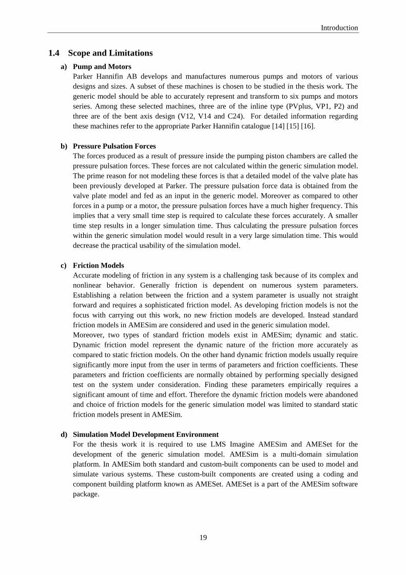
1.4 Scope and Limitations
a) Pump and Motors
Parker Hannifin AB develops and manufactures numerous pumps and motors of various
designs and sizes. A subset of these machines is chosen to be studied in the thesis work. The
generic model should be able to accurately represent and transform to six pumps and motors
series. Among these selected machines, three are of the inline type (PVplus, VP1, P2) and
three are of the bent axis design (V12, V14 and C24). For detailed information regarding
these machines refer to the appropriate Parker Hannifin catalogue [14] [15] [16].
b) Pressure Pulsation Forces
The forces produced as a result of pressure inside the pumping piston chambers are called the
pressure pulsation forces. These forces are not calculated within the generic simulation model.
The prime reason for not modeling these forces is that a detailed model of the valve plate has
been previously developed at Parker. The pressure pulsation force data is obtained from the
valve plate model and fed as an input in the generic model. Moreover as compared to other
forces in a pump or a motor, the pressure pulsation forces have a much higher frequency. This
implies that a very small time step is required to calculate these forces accurately. A smaller
time step results in a longer simulation time. Thus calculating the pressure pulsation forces
within the generic simulation model would result in a very large simulation time. This would
decrease the practical usability of the simulation model.
c) Friction Models
Accurate modeling of friction in any system is a challenging task because of its complex and
nonlinear behavior. Generally friction is dependent on numerous system parameters.
Establishing a relation between the friction and a system parameter is usually not straight
forward and requires a sophisticated friction model. As developing friction models is not the
focus with carrying out this work, no new friction models are developed. Instead standard
friction models in AMESim are considered and used in the generic simulation model.
Moreover, two types of standard friction models exist in AMESim; dynamic and static.
Dynamic friction model represent the dynamic nature of the friction more accurately as
compared to static friction models. On the other hand dynamic friction models usually require
significantly more input from the user in terms of parameters and friction coefficients. These
parameters and friction coefficients are normally obtained by performing specially designed
test on the system under consideration. Finding these parameters empirically requires a
significant amount of time and effort. Therefore the dynamic friction models were abandoned
and choice of friction models for the generic simulation model was limited to standard static
friction models present in AMESim.
d) Simulation Model Development Environment
For the thesis work it is required to use LMS Imagine AMESim and AMESet for the
development of the generic simulation model. AMESim is a multi-domain simulation
platform. In AMESim both standard and custom-built components can be used to model and
simulate various systems. These custom-built components are created using a coding and
component building platform known as AMESet. AMESet is a part of the AMESim software
package.

Introduction
20
e) User Interface and Parameter Library Environment
If possible, it is required to use MS Excel as the platform for developing and creating both the
user interface and the parameter library. The software’s ability to handle large amounts of data
and abundant knowledge among the potential users are the two prime reasons for its selection.
1.5 Motivation
A generic simulation model offers a series of advantages over the traditional method of model
development. These significant advantages that can be gained through the use of a generic simulation
model are the prime motivation behind its development. Some of the advantages of using a generic
simulation model to represent hydraulic pumps and motors are listed below.
a) Common Model Structure
Through the use of a generic simulation model, multiple pumps and motors can be modeled
using the same structure. This is demonstrated in this work by using a single generic
simulation model to represent both inline and bent axis pumps and motors.
b) Easier Comparison
By using the generic structure, it is easier to compare different pumps and motors. As all of
them are based on the same structure, it is easier to find out the similarities and differences in
pumps and motors of various sizes or types.
c) Shorter Startup Time
The generic model enables automated model creation of different pumps and motors resulting
in shorter startup time for performing a simulation or an analysis. This also enables the
designer to spend less time on model development and more on performing simulation and
analysis.
d) Less File Management
The generic simulation model requires only a relatively smaller number of files to operate as
opposed to large number of files resulting from traditional models. This is due to the fact that
multiple machines can be modeled using a single generic model while traditional modeling
techniques require that each and every machine has its own individual model file. Due to less
number of files to deal with, the task of maintaining, tracking of all the revisions and updating
the simulation model requires significantly less effort and time as compared to traditional
modeling methodologies.
e) Standard Procedure
A standard way of model development can be adopted through the use of a generic simulation
model. Subsequent to the development and finalization of the basic structure for the generic
simulation model, all pumps and motors can be modeled using the same model structure.
Same model structure implies that similar steps are needed to be performed in order to develop
a simulation model for a pump or a motor. So when using a generic simulation model the steps
in the model development process remain the same, thus a standard procedure for simulation
model development can be introduced.

Introduction
21
f) Cost Reduction
Incorporating a generic simulation model into the design process would lead to a reduction in
development costs. A generic simulation model offers the capability of automated model
creation and modification thus decreasing the time and cost required for developing and
modifying a simulation model.
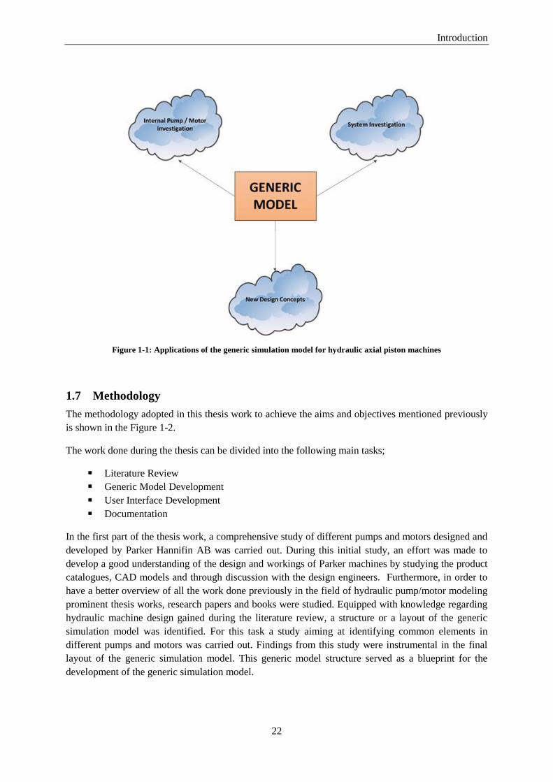
1.6 Application
Intended application of a simulation model contributes heavily towards the final model structure and
design. Therefore, before the commencement of the model development process it is vitally important
to outline how and where a simulation model is intended to be used. The generic simulation model of
hydraulic axial piston machines developed and implemented as part of this thesis work is envisioned
to be used in three distinct scenarios illustrated in Figure 1-1.
1.6.1 Internal Pump/Motor Investigation
The generic model can be used for studying the internal workings of a pump or a motor referred here
as an internal pump/motor investigation. In this role, the generic model can be used to study the
individual design, performance and dynamics of pump or motor components. Through sensitivity
analysis, the contribution of individual component performance in the overall pump/motor
performance can be investigated. Inversely, similar techniques can be used to analyze the effect of
pump/motor parameters on the performance of a component. As an example, it might be of interest to
investigate the amount of forces or torques generated by the setting piston by changing the setting
piston dimension or to study the minimum setting time achievable by changing the flow entering the
setting piston chamber etc. Moreover, interaction of components among each other within a
pump/motor can also be studied.
1.6.2 System Investigation
The same generic model can be used for performing system level investigations. In this role, the inner
working of the pump or motor model are not of interest but rather how the pump or motor performs
and interacts with other components in a system is of value. For example, a system investigation may
be performed on a hydraulic system comprising of many pumps and motors along with other
components such as valves, prime movers, loads etc. In such a system all these pumps and motor can
be modeled using the generic model. Furthermore, as an optional feature the internal workings of the
generic model can be locked, so that they are not visible or accessible during a system level
investigation. In essence the generic model acts as a black box in this case. Such a feature is helpful in
protecting confidential data and design when such an investigation is needed to be performed by a
customer.
1.6.3 New Design Concepts
The generic model can be used for designing and testing new concepts for pumps and motors. As the
generic model is built in a standardized manner, new types of pumps and motors can be studied,
simulated and analyzed with minimum modification to the generic model.
Introduction
22
Figure 1-1: Applications of the generic simulation model for hydraulic axial piston machines
1.7 Methodology
The methodology adopted in this thesis work to achieve the aims and objectives mentioned previously
is shown in the Figure 1-2.
The work done during the thesis can be divided into the following main tasks;
Literature Review
Generic Model Development
User Interface Development
Documentation
In the first part of the thesis work, a comprehensive study of different pumps and motors designed and
developed by Parker Hannifin AB was carried out. During this initial study, an effort was made to
develop a good understanding of the design and workings of Parker machines by studying the product
catalogues, CAD models and through discussion with the design engineers. Furthermore, in order to
have a better overview of all the work done previously in the field of hydraulic pump/motor modeling
prominent thesis works, research papers and books were studied. Equipped with knowledge regarding
hydraulic machine design gained during the literature review, a structure or a layout of the generic
simulation model was identified. For this task a study aiming at identifying common elements in
different pumps and motors was carried out. Findings from this study were instrumental in the final
layout of the generic simulation model. This generic model structure served as a blueprint for the
development of the generic simulation model.

Introduction
23
Figure 1-2: Breakdown of the master thesis work
During the generic model development, all the internal components necessary for the true
representation of the hydraulic machines under consideration were modeled. Development of the
generic simulation model was preceded by its validation in order to judge the accuracy of its results.
The validation was performed by comparing the simulation model results with the experimental
measurements. In order to have the same physical and simulated systems, simulation models of some
pump/motor controllers were also developed during this validation phase. So, these simulation models
of the pump/motor controllers were coupled with the generic simulation model of pump/motors to
perform the validation.
Alongside the development of the generic simulation model a user-interface was also developed. This
user interface enables the user to communicate with generic model. Development of this user interface
also included development of a parameter library. This parameter library serves a database of all the
inputs required by the generic simulation model. Finally to document the generic simulation model, a
complete help section was created for every component created in AMESim.

Theory
25
2 Theory
2.1 Displacement Machines: Working principle
Hydraulic pumps are positive displacement devices. This positive displacement is achieved in two
steps; firstly the fluid enters a cavity through the suction side which has an expanding cavity, and
leaves it at the discharge side, which has a decreasing cavity.
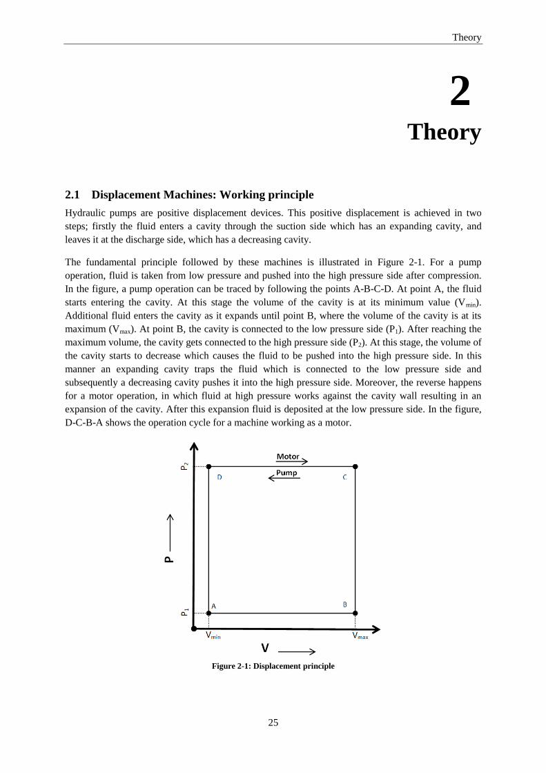
The fundamental principle followed by these machines is illustrated in Figure 2-1. For a pump
operation, fluid is taken from low pressure and pushed into the high pressure side after compression.
In the figure, a pump operation can be traced by following the points A-B-C-D. At point A, the fluid
starts entering the cavity. At this stage the volume of the cavity is at its minimum value (Vmin).
Additional fluid enters the cavity as it expands until point B, where the volume of the cavity is at its
maximum (Vmax). At point B, the cavity is connected to the low pressure side (P1). After reaching the
maximum volume, the cavity gets connected to the high pressure side (P2). At this stage, the volume of
the cavity starts to decrease which causes the fluid to be pushed into the high pressure side. In this
manner an expanding cavity traps the fluid which is connected to the low pressure side and
subsequently a decreasing cavity pushes it into the high pressure side. Moreover, the reverse happens
for a motor operation, in which fluid at high pressure works against the cavity wall resulting in an
expansion of the cavity. After this expansion fluid is deposited at the low pressure side. In the figure,
D-C-B-A shows the operation cycle for a machine working as a motor.
Figure 2-1: Displacement principle

Theory
26
2.2 Types of Pumps and Motors
The fundamental working principle of hydraulic displacement machines described above could be
realized through a large number of designs. A classification of the hydraulic machines could be done
based on their design to achieve the aforementioned displacement principle. Figure 2-2 provides an
overview for such a classification. This thesis work focuses on the development of simulation models
of swash plate/inline and bent axis pump/motors which are a subcategory of axial piston machines.
Figure 2-2: Classification of hydrostatic machines (adapted from [1])

Theory
27
2.3 Axial Piston Pumps and Motors
This thesis work is limited to the study of axial piston machines; therefore a brief description of the
internal design of these machines is presented here. From the Figure 2-2 we can see that axial piston
machines are divided into two main types; inline and bent axis. In both of these machines, pistons are
radially arranged in a cylinder barrel. In the pump operation, the reciprocating linear motion of these
pistons causes suction of fluid at the low pressure and its delivery at the high pressure port. The
mechanical energy to rotate these pistons is delivered by a prime mover through a mechanical shaft.
These machines can have either fixed or variable displacement. For a fixed pump the output flow
remains constant for a given rotational speed, on the other hand in a variable pump this flow could be
changed by altering the pump displacement. In an inline machine the pumping pistons slide against a
plate called the swash plate. The angle of the swash plate determines the displacement and
consequently the flow output of a pump. While in a bent axis machine the angle between the
mechanical shaft and the cylinder barrel determines the displacement of the machine. In variable
displacement machines the angle of the swash plate or the barrel assembly is set by a piston called the
setting piston. The movement of this setting piston is controlled by a compensator or controller. This
controller based on the current system parameters (e.g. system pressure) and the desired type of
control (e.g. constant pressure) directs appropriate flow into the setting piston chamber causing the
movement of the setting piston.
Another important component in these machines is the valve plate. The valve plate lies in between the
cylinder barrel and the inlet/outlet ports. Hydraulic fluid entering the barrel through the inlet port or
the fluid going out from the barrel into the outlet port passes through the cavities of the valve plate.
The design of these cavities on the valve plate greatly affects the performance of a machine.
Moreover, at startup the pressure in the system is low implying that the controller is unable to set the
displacement of the pump. Therefore, in pumps a spring called the servo spring is attached to the
swash plate to stroke up the pump at startup.
In the case of a motor operation, high pressure fluid enters the machine causing a reciprocating motion
of the pistons in the cylinder barrel. This in turn rotates the mechanical shaft which results in an output
speed and torque. Theoretically, most hydraulic machines can be used as both pump and motor,
however to achieve an optimal design, machines are specifically designed to work as either a pump or
a motor. Hydraulic machines are normally classified by their maximum displacement, operating
pressure and speed.
Figure 2-3: Axial piston (a) inline (b) bent axis machine
Theory
28
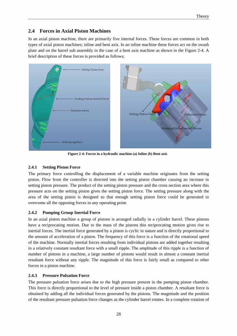
2.4 Forces in Axial Piston Machines
In an axial piston machine, there are primarily five internal forces. These forces are common in both
types of axial piston machines; inline and bent axis. In an inline machine these forces act on the swash
plate and on the barrel sub assembly in the case of a bent axis machine as shown in the Figure 2-4. A
brief description of these forces is provided as follows;
Figure 2-4: Forces in a hydraulic machine (a) Inline (b) Bent axis
2.4.1 Setting Piston Force
The primary force controlling the displacement of a variable machine originates from the setting
piston. Flow from the controller is directed into the setting piston chamber causing an increase in
setting piston pressure. The product of the setting piston pressure and the cross section area where this
pressure acts on the setting piston gives the setting piston force. The setting pressure along with the
area of the setting piston is designed so that enough setting piston force could be generated to
overcome all the opposing forces in any operating point.
2.4.2 Pumping Group Inertial Force
In an axial piston machine a group of pistons is arranged radially in a cylinder barrel. These pistons
have a reciprocating motion. Due to the mass of the pistons this reciprocating motion gives rise to
inertial forces. The inertial force generated by a piston is cyclic in nature and is directly proportional to
the amount of acceleration of a piston. The frequency of this force is a function of the rotational speed
of the machine. Normally inertial forces resulting from individual pistons are added together resulting
in a relatively constant resultant force with a small ripple. The amplitude of this ripple is a function of
number of pistons in a machine, a large number of pistons would result in almost a constant inertial
resultant force without any ripple. The magnitude of this force is fairly small as compared to other
forces in a piston machine.
2.4.3 Pressure Pulsation Force
The pressure pulsation force arises due to the high pressure present in the pumping piston chamber.
This force is directly proportional to the level of pressure inside a piston chamber. A resultant force is
obtained by adding all the individual forces generated by the pistons. The magnitude and the position
of the resultant pressure pulsation force changes as the cylinder barrel rotates. In a complete rotation of

Theory
29
the barrel, the resultant forces moves in a distinct pattern closely resembling the digit ´8´. The
magnitude of the resultant force is large and is comparable to the maximum setting piston force.
2.4.4 Servo Spring Force
The servo spring force originates from a spring attached to the swash plate in an inline pump. This
spring is placed to mechanically upstroke the pump at start up when the system pressure is not enough
to generate any significant setting force. Servo springs are normally only found in pumps. The
magnitude of this force during steady state condition is small and is somewhat comparable to the
pumping group inertial resultant force.
2.4.5 Frictional Forces
As with any system with moving parts, friction forces also exist in hydraulic machines. A friction
force is associated with every component that moves against a surface in a hydraulic machine however
the major sources of frictional forces in an inline machine are the swash plate moving against the
concave shaped cradle, movement of the setting piston in its chamber and rotation of the cylinder
barrel against the valve plate. In the case of a bent axis machine the prime sources of friction forces
are movement of barrel sub assembly, setting piston and the rotation of barrel against the valve plate.
Generally the machines are designed to provide oil between these sliding or rotating surfaces in order
to reduce the frictional forces. The magnitude of frictional forces is highly dependent on the running
conditions of the machine.


3 Approach &
Implementation
3.1 Identify Common Elements
In order to identify a simulation model structure for the development of the generic simulation model,
a study was carried out to identify the common elements and features that are present in different types
of pumps and motors.
3.1.1 Setting Piston
The setting piston sub-assembly along with components connecting the setting piston to the swash
plate or the barrel sub assembly used in pumps and motors under consideration are shown in Figure
3-1.
Figure 3-1: Setting piston mechanism (a) PVplus (b) VP1 (c) P2 (d) V14 (e) C24

Approach & Implementation
32
A closer look at the various pumps and motors shown in the figure above reveals the following three
distinct common features.
Piston
Inertia
Connection Mechanism
From the figure it can be clearly seen that a setting piston is connected to either a swash plate or a
barrel sub assembly via a connection mechanism. At a fundamental level a swash plate and the barrel
sub assembly are same as both can be thought of as an inertia. The force generated by the setting
piston is transferred to the swivel inertia through a connection mechanism. This connection
mechanism is the only element in the assemblies shown above which varies in design. This connection
mechanism translates the force and the linear movement of the setting piston into an equivalent torque
and rotation of the swivel inertia respectively.
3.1.2 Servo Spring
Figure 3-2 shows the servo spring along with components connecting the servo spring with the swash
plate present in hydraulic machines under consideration.
Figure 3-2: Servo spring mechanism (a) PVplus (b) P2 (c) VP1
Similar to the setting piston assemblies, the following three common components or features can be
identified in the figure shown above.
Spring
Inertia
Connection Mechanism
A connection mechanism connects the servo spring to swivel inertia. This connection mechanism
transforms the force generated by the servo spring into an equivalent torque acting on the swivel
inertia. Like in the case of the setting piston mechanism, this servo spring connection mechanism is
the only component varying in design when comparing servo spring assemblies of different pumps
under consideration.

Approach & Implementation
33
3.1.3 Pumping Group
The pumping piston groups present in pumps/motors under consideration are shown in Figure 3-3
along with the components fixing it to the swash plate or the yoke sub assembly. As mentioned earlier,
both pumping piston inertial forces and pressure pulsation forces originate from the pumping piston
group.
Figure 3-3: Stroking piston group (a) PVplus (b) P2 (c) VP1 (d) C24
The following three common elements can be identified from the figure above.
Pumping Group
Inertia
Connection Mechanism
Similar to the previous two cases, the pumping group is connected to the swivel inertia through a
connection mechanism. Also identical to the setting piston and servo spring assemblies, this
connection mechanism varies in design among different pump/motors.
From the above brief investigation, elements that are common and varying in pumps/motors under
consideration can be identified.

Approach & Implementation
34
3.2 Generic Model
3.2.1 Definition
From the above discussion, we can conclude that a simulation model capable of representing pumps
and motors of various sizes and designs requires the following characteristics;
a) Parametric
Among different machines belonging to the same pump or a motor series, the design of the
components remains the same. The components in this case only differ in size. Therefore, a
simulation model should be parametric to be able to represent different machine sizes from the
same pump or motor series. So, by changing these parameters values the model can convert
from one machine size to another. This conversion is represented in Figure 3-4(a).
b) Transformable
While comparing two machines from different pump or motor series the design of some of
their components also differ. Therefore, in the case where the simulation model needs to able
to represent machines from two or more different series, it needs to be able to transform.
Transformation of a simulation model is represented in Figure 3-4(b).
So a generic model in this context can be defined as a model that is parametric and has the ability to
transform to some extent.
Figure 3-4: Generic model (a) Parametric change (b) Transformation

Approach & Implementation
35
3.2.2 Structure: Modular Approach
The methodology used to develop a generic simulation model can be termed as modular. In this
modular approach every connection mechanism identified in the previous section is considered as a
module. Figure 3-5 shows a connection mechanism which connects the setting piston with the swivel
inertia in an inline pump. This connection mechanism is modeled as a single module.
Figure 3-5 Modular approach
These modules are connected together to form the generic simulation model. As mentioned
previously, for a simulation model to be generic it should be parametric and capable of transformation.
Therefore, if all the modules making up the simulation model are parametric and transformable then
the entire simulation model consequently becomes parametric and transformable. This in turn implies
that the simulation model is generic. So the task of developing a generic simulation model boils down
to making all of its constituent modules generic. Figure 3-6 shows an example of a parametric and
transformation of a setting piston mechanism module.
Figure 3-6: Figure 3 6: Module (a) Parametric change (b) Transformation example
Figure 3-7 shows the conceptual representation of the generic simulation model. The modules in the
simulation model can be roughly divided into three main categories; force source modules, connection
mechanism modules, inertia module.
The components in a hydraulic machine generating a force are referred here as force source modules.
From the figure, we can see that these force sources are setting piston, inertia of the pumping piston
group, pressure pulsation and servo spring. The force generated by these force source modules is fed
into connection mechanism modules. These connection modules transform the input force into an
equivalent output torque. The output torques generated by the connection mechanisms are applied on
the swivel inertia. This swivel inertia is roughly equivalent to the inertia of the swash plate in an inline

Approach & Implementation
36
type machine while for bent axis type machine this inertia represents the inertia of the barrel sub
assembly. The rotation angle and velocity of the swivel inertia is also fed back to the connection
mechanism where it is converted into an equivalent linear displacement and velocity. This linear
displacement and velocity is then applied on the force source modules. Figure 3-7 also highlights the
fact that the only difference between the simulation models for two different machines is the
connection mechanism modules. These connection mechanism modules can be changed parametrically
or replaced by other connection mechanism modules to transform the simulation model from one
machine to another.
Figure 3-7: Conceptual representation of the generic simulation model

Approach & Implementation
37
3.2.3 Software
The software used for the development of the generic simulation model is the LMS AMESim.
AMESim is a multi domain simulation platform for modeling and analyzing one dimensional systems.
The AMESim simulation package includes a number of validated standard component libraries for
different physical domains like mechanical, hydraulics, electromechanical etc. The components from
diverse domains can be joined together to form a complex simulation model of a complete system.
Alongside the pre built component libraries, AMESim also provides the capability to create and
develop custom libraries. For creating custom component libraries a coding and component creation
platform known as AMESet can be used.
Furthermore AMESim is also able to communicate with numerous other softwares like MATLAB,
Simulink and Microsoft Excel etc. Through the use of VBA scripting and AMESim API many task
can be automated. AMESim also provides scripting interface using Python, C++ and Visual Basic
languages.
Due to these aforementioned features AMESim is an ideal simulation platform for modeling
mechatronic systems like a hydraulic pump/motor. In addition to that the existence of the AMESim
API and ability to communicate with MS Excel also makes it a suitable tool for automated
modification and transformation of the generic simulation model.
Figure 3-8: LMS AMESim [17]
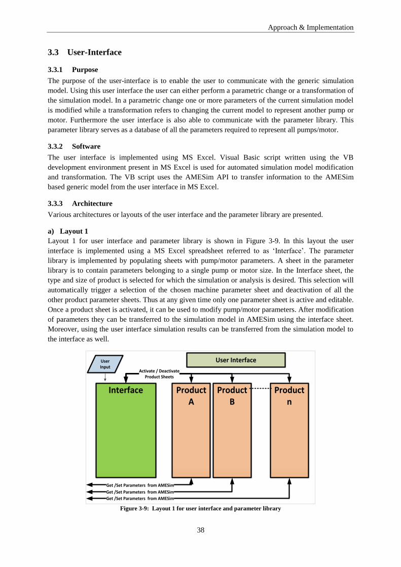
Approach & Implementation
38
3.3 User-Interface
3.3.1 Purpose
The purpose of the user-interface is to enable the user to communicate with the generic simulation
model. Using this user interface the user can either perform a parametric change or a transformation of
the simulation model. In a parametric change one or more parameters of the current simulation model
is modified while a transformation refers to changing the current model to represent another pump or
motor. Furthermore the user interface is also able to communicate with the parameter library. This
parameter library serves as a database of all the parameters required to represent all pumps/motor.
3.3.2 Software
The user interface is implemented using MS Excel. Visual Basic script written using the VB
development environment present in MS Excel is used for automated simulation model modification
and transformation. The VB script uses the AMESim API to transfer information to the AMESim
based generic model from the user interface in MS Excel.
3.3.3 Architecture
Various architectures or layouts of the user interface and the parameter library are presented.
a) Layout 1
Layout 1 for user interface and parameter library is shown in Figure 3-9. In this layout the user
interface is implemented using a MS Excel spreadsheet referred to as ‘Interface’. The parameter
library is implemented by populating sheets with pump/motor parameters. A sheet in the parameter
library is to contain parameters belonging to a single pump or motor size. In the Interface sheet, the
type and size of product is selected for which the simulation or analysis is desired. This selection will
automatically trigger a selection of the chosen machine parameter sheet and deactivation of all the
other product parameter sheets. Thus at any given time only one parameter sheet is active and editable.
Once a product sheet is activated, it can be used to modify pump/motor parameters. After modification
of parameters they can be transferred to the simulation model in AMESim using the interface sheet.
Moreover, using the user interface simulation results can be transferred from the simulation model to
the interface as well.
Interface Product A
Product B
Product n
Activate / DeactivateProduct Sheets
Get /Set Parameters from AMESim
Get /Set Parameters from AMESim
Get /Set Parameters from AMESim
UserInput
User Interface
Figure 3-9: Layout 1 for user interface and parameter library
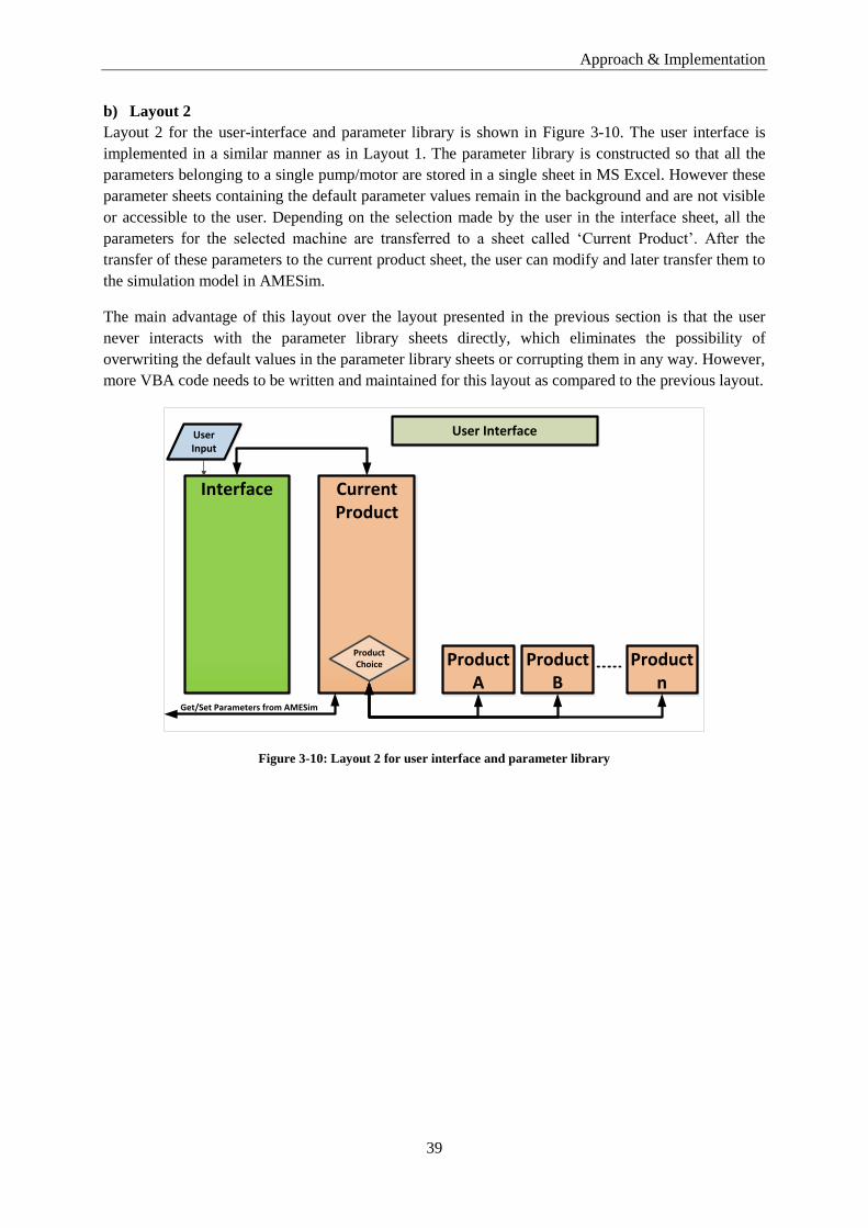
Approach & Implementation
39
b) Layout 2
Layout 2 for the user-interface and parameter library is shown in Figure 3-10. The user interface is
implemented in a similar manner as in Layout 1. The parameter library is constructed so that all the
parameters belonging to a single pump/motor are stored in a single sheet in MS Excel. However these
parameter sheets containing the default parameter values remain in the background and are not visible
or accessible to the user. Depending on the selection made by the user in the interface sheet, all the
parameters for the selected machine are transferred to a sheet called ‘Current Product’. After the
transfer of these parameters to the current product sheet, the user can modify and later transfer them to
the simulation model in AMESim.
The main advantage of this layout over the layout presented in the previous section is that the user
never interacts with the parameter library sheets directly, which eliminates the possibility of
overwriting the default values in the parameter library sheets or corrupting them in any way. However,
more VBA code needs to be written and maintained for this layout as compared to the previous layout.
Interface CurrentProduct
Product A
Product B
Product n
User Interface
Product Choice
UserInput
Get/Set Parameters from AMESim
Figure 3-10: Layout 2 for user interface and parameter library

Approach & Implementation
40
3.3.3.1 Chosen/Implemented Layout
The chosen/implemented layout of the user-interface and parameter library is shown in the Figure
3-11.
Figure 3-11: Implemented layout of user interface and parameter library
In the chosen layout, the user interacts with the generic model in AMESim through the ‘User
Interface’. Moreover the user interface also serves a bridge between the parameter library and the
generic model. The type and size of pump or motor can be selected in the interface sheet. The interface
sheet contains buttons for the transformation of the generic model into specific pump or motor model
and also for setting and modifying the parameters.
Furthermore, the parameter library is implemented by accumulating all the parameters belonging to a
pump or a motor in separate sheets. These parameter sheets are populated using the CAD models and
after populating they should be made read-only to avoid modifying the default parameters by mistake.
Once the type and size of the pump or motor is selected, the parameters from individual pump or
motor parameter sheet are transferred to the current model sheet. All the required modification in the
parameter values are to be done in the current model sheet. This will prevent the user from overwriting
the default parameters in the parameter library sheets.
Population of Parameter Library
In order to create a simulation model of a pump or motor, equations are required which
mathematically describe the different components. These equations then in turn require parameters as
inputs. The geometrical parameters required in the AMESim simulation model are extracted from the
CAD models in Pro-E. While extracting properties like inertia it is important that the reference in the
CAD and simulation model is the same. To keep things simple and intuitive, a global coordinate
system is defined. All the properties are measured with reference to this global coordinate system. The
parameters collected from CAD models are used to populate the parameter library in the user-
interface.
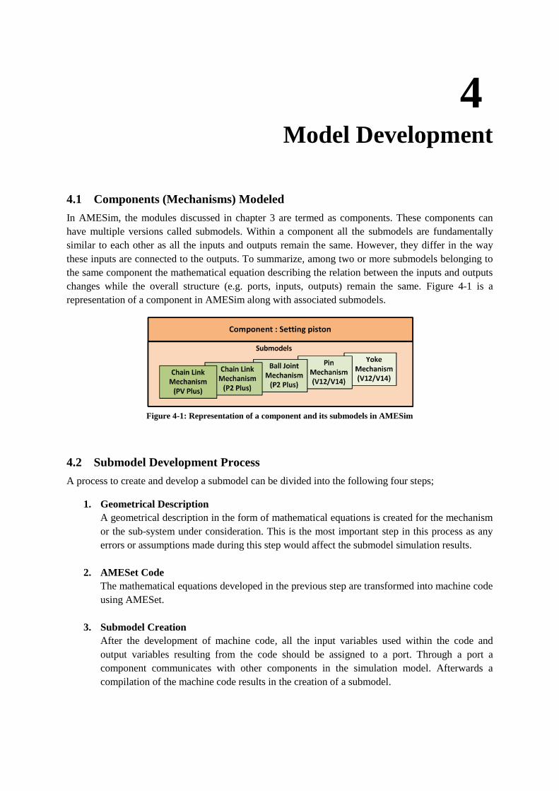
4 Model Development
4.1 Components (Mechanisms) Modeled
In AMESim, the modules discussed in chapter 3 are termed as components. These components can
have multiple versions called submodels. Within a component all the submodels are fundamentally
similar to each other as all the inputs and outputs remain the same. However, they differ in the way
these inputs are connected to the outputs. To summarize, among two or more submodels belonging to
the same component the mathematical equation describing the relation between the inputs and outputs
changes while the overall structure (e.g. ports, inputs, outputs) remain the same. Figure 4-1 is a
representation of a component in AMESim along with associated submodels.
Figure 4-1: Representation of a component and its submodels in AMESim
4.2 Submodel Development Process
A process to create and develop a submodel can be divided into the following four steps;
1. Geometrical Description
A geometrical description in the form of mathematical equations is created for the mechanism
or the sub-system under consideration. This is the most important step in this process as any
errors or assumptions made during this step would affect the submodel simulation results.
2. AMESet Code
The mathematical equations developed in the previous step are transformed into machine code
using AMESet.
3. Submodel Creation
After the development of machine code, all the input variables used within the code and
output variables resulting from the code should be assigned to a port. Through a port a
component communicates with other components in the simulation model. Afterwards a
compilation of the machine code results in the creation of a submodel.

Model Development
42
4. Component Assignment
In AMESim every submodel should belong to a component. Therefore, the submodel created
in the previous step is assigned to an appropriate component in AMESim. At this stage, this
component and the submodel can be used in a similar way as a standard AMESim component
or submodel.
Figure 4-2: Submodel development process

Model Development
43
4.3 Equation development
4.3.1 Inline Axial Piston Pumps
The following three inline axial piston pumps are modeled.
1. PVplus
2. VP1
3. P2
4.3.2 PVplus
4.3.2.1 Introduction
PVplus is a variable inline axial piston pump. It is designed for industrial applications. The
displacement for this pump ranges from 16 to 360 . Refer to Parker Hannifin
catalogue # HY30-3245/UK for detailed information on PVplus series of pumps.
4.3.2.2 Component (Mechanism) Equations
4.3.2.2.1 Setting Piston Mechanism
a) Equations
Setting Piston Displacement
Equations describing the displacement of the setting piston for a given swivel angle are presented
below. Figure 4-3 illustrates the trigonometry diagram used for the calculation of the setting piston
displacement.
Figure 4-3: Setting piston displacement (PVplus)
In the figure above, point C is the point of rotation for the swivel inertia. This point is also the origin
for the coordinate system i.e;
Coordinates of point A (w.r.t point C)

Model Development
44
Coordinates of B (w.r.t point C)
The length of the chain remains constant, therefore from the geometry we can write;
Putting in the values of A and B gives;
Solving for disp;
Ignoring the negative term gives the following equation describing the displacement of the setting
piston.
Where R is calculated as follows;
And theta ( ) is calculated as

Model Development
45
Setting Piston Velocity
The velocity of the setting piston can be calculated using the set of equations presented below. Figure
4-4 shows the trigonometry diagram used for these equations.
Figure 4-4: Setting piston velocity (PVplus)
From the figure above, we have;
Here point serves as the instantaneous center of velocity, from that we can write;
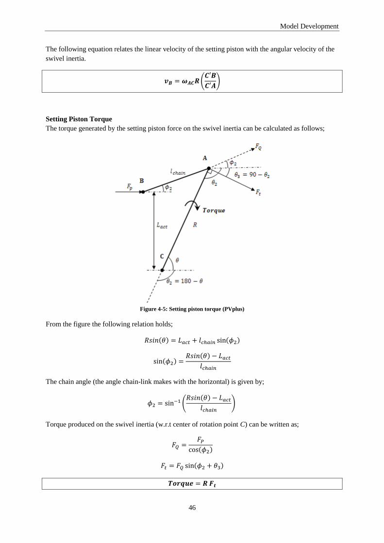
Model Development
46
The following equation relates the linear velocity of the setting piston with the angular velocity of the
swivel inertia.
Setting Piston Torque
The torque generated by the setting piston force on the swivel inertia can be calculated as follows;
Figure 4-5: Setting piston torque (PVplus)
From the figure the following relation holds;
The chain angle (the angle chain-link makes with the horizontal) is given by;
Torque produced on the swivel inertia (w.r.t center of rotation point C) can be written as;

Model Development
47
b) Inputs
The inputs that are required for the setting piston mechanism are,
Radius of the Swash plate - Rswash [mm]
Horizontal distance from Swash circular endpoint to Chain attachment point - dess [mm]
Distance between Chain attachment point on Swash plate to Point S prime -dl2S [mm]
Vertical distance from rotation axis to center of Setting Piston - Lact [mm]
Length of the chain - lchain [mm]
Mass of setting piston + chain link - m [kg]
Mass of the setting Piston - [kg]
Mass of the chain link - [kg]
c) Parameters
The parameters that are required for the calculation of the setting piston displacement, velocity and
torque are shown using the CAD models in Figure 4-6 and Figure 4-7.
Figure 4-6: Setting piston mechanism dimensions (PVplus)
Figure 4-7: Setting piston dimension (PVplus)

Model Development
48
4.3.2.2.2 Servo Spring
a) Equations
The equations describing the compression of the servo spring for a given swivel angle in PV plus
machine are presented below. Moreover equations describing the force and the corresponding torque
generated due the compression of the spring are also presented. Figure 4-8 shows the trigonometry
diagram used for the formulation of these equations.
Figure 4-8: Servo spring compression (PVplus)
From the figure, we can see that
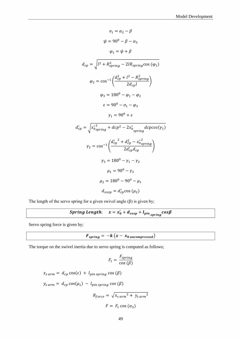
Model Development
49
The length of the servo spring for a given swivel angle (β) is given by;
Servo spring force is given by;
The torque on the swivel inertia due to servo spring is computed as follows;

Model Development
50
b) Inputs
The inputs that are required are,
Spring Constant - k [N/m]
Radius of the Swash Plate - d1 [mm]
Horizontal distance from the Swash plate circular edge to Pin attachment point - d3 [mm]
Distance between Pin attachment point to point S - dsspring [mm]
Pin Length - lpinspring [mm]
Horizontal distance between Initial spring length (beta = 0) and Center of rotation -
x0primespring [mm]
Initial spring length- x0prime [mm]
Uncompressed length of the spring - x0uncompressed [mm]
c) Parameters
The parameters that are required for the calculation of the servo spring compression, force and torque
are shown in Figure 4-9.
Figure 4-9: Servo spring dimensions (PVplus)

Model Development
51
4.3.2.2.3 Stroking pistons inertial forces
a) Equations
Equations describing the inertial forces and the torque acting on the swivel inertia due to these forces
are presented below. Figure 4-10 illustrates the parameters used in these equations.
Figure 4-10: Stroking piston inertial forces in inline machine (corutesy Parker Hannifin AB)
For a stroking piston the force produced due to its inertia can be written as;
The acceleration of a piston during its stroke can be calculated as follows;
Taking the derivative of the above equation twice gives acceleration;
The moment produced by this inertial force on the swivel inertia can be written as;
The moment arm is given by;
Where

Model Development
52
The total torque due to inertia of all the pumping pistons at an instance is given by;
b) Inputs
The inputs that are required are listed as follows;
Barrel Radius - Rb [mm]
Mass of one piston- mp [kg]
Total number of pistons - nt [null]
Inertia of Barrel + shaft - J [kg*m^2]
c) Parameters
The parameter that is required is shown in Figure 4-11.
Figure 4-11: Barrel radius (PVplus)
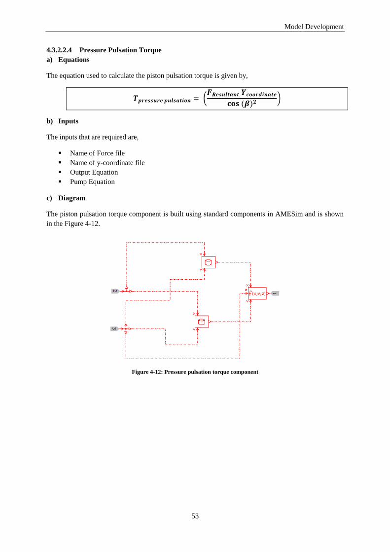
Model Development
53
4.3.2.2.4 Pressure Pulsation Torque
a) Equations
The equation used to calculate the piston pulsation torque is given by,
b) Inputs
The inputs that are required are,
Name of Force file
Name of y-coordinate file
Output Equation
Pump Equation
c) Diagram
The piston pulsation torque component is built using standard components in AMESim and is shown
in the Figure 4-12.
Figure 4-12: Pressure pulsation torque component
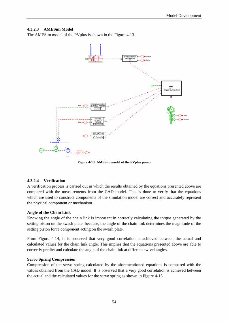
Model Development
54
4.3.2.3 AMESim Model
The AMESim model of the PVplus is shown in the Figure 4-13.
Figure 4-13: AMESim model of the PVplus pump
4.3.2.4 Verification
A verification process is carried out in which the results obtained by the equations presented above are
compared with the measurements from the CAD model. This is done to verify that the equations
which are used to construct components of the simulation model are correct and accurately represent
the physical component or mechanism.
Angle of the Chain Link
Knowing the angle of the chain link is important in correctly calculating the torque generated by the
setting piston on the swash plate, because, the angle of the chain link determines the magnitude of the
setting piston force component acting on the swash plate.
From Figure 4-14, it is observed that very good correlation is achieved between the actual and
calculated values for the chain link angle. This implies that the equations presented above are able to
correctly predict and calculate the angle of the chain link at different swivel angles.
Servo Spring Compression
Compression of the servo spring calculated by the aforementioned equations is compared with the
values obtained from the CAD model. It is observed that a very good correlation is achieved between
the actual and the calculated values for the servo spring as shown in Figure 4-15.
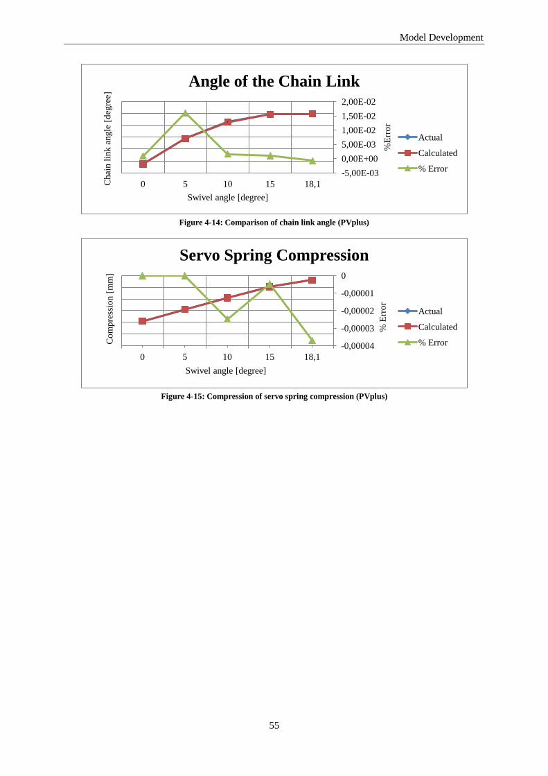
Model Development
55
Figure 4-14: Comparison of chain link angle (PVplus)
Figure 4-15: Compression of servo spring compression (PVplus)
-5,00E-03
0,00E+00
5,00E-03
1,00E-02
1,50E-02
2,00E-02
-6
-4
-2
0
2
4
6
0 5 10 15 18,1
%E
rro
r
Chai
n l
ink a
ngle
[d
egre
e]
Swivel angle [degree]
Angle of the Chain Link
Actual
Calculated
% Error
-0,00004
-0,00003
-0,00002
-0,00001
0
160
170
180
190
200
210
220
0 5 10 15 18,1
% E
rro
r
Co
mp
ress
ion [
mm
]
Swivel angle [degree]
Servo Spring Compression
Actual
Calculated
% Error

Model Development
56
4.3.3 VP1
4.3.3.1 Introduction
VP1 is a variable inline axial piston pump. It is mainly intended for truck applications. This pump
series is available in four different sizes ranging from 45 to 120 . For more
information on VP1 series pumps features and typical applications refer to Parker Hannifin catalogue
HY30-8200/UK.
4.3.3.2 Component (Mechanism) Equations
4.3.3.2.1 Upper Setting Piston Mechanism
a) Equations
The equations describing the upper setting piston displacement, velocity and torque are presented
below. Figure 4-16 shows the trigonometry diagram used for the formulation of these equations.
Figure 4-16: Upper setting piston displacement and torque (VP1)
The angle of upper setting piston at a given swivel angle (β) is given by;
Torque generated by the upper setting piston acting on the swivel angle is given by;

Model Development
57
Displacement of the piston is given by;
Velocity of the upper setting piston is given by derivative of the displacement;
b) Inputs
The inputs required for the above equations are listed as follows,
β
β –
c) Parameters
The parameters listed above are shown in Figure 4-17 and Figure 4-18.
Figure 4-17: Upper setting piston mechanism dimensions (VP1)
Figure 4-18: Upper setting piston dimensions (VP1)

Model Development
58
4.3.3.2.2 Lower Setting Piston Mechanism
a) Equations
The equations describing the lower setting piston displacement, velocity and torque are presented
below. Figure 4-19 shows the trigonometry diagram used for the formulation of these equations.
Figure 4-19: Lower setting piston displacement and torque (VP1)
Torque generated by the lower setting piston acting on the swivel inertia is given by;
Displacement of the lower setting piston is given by;
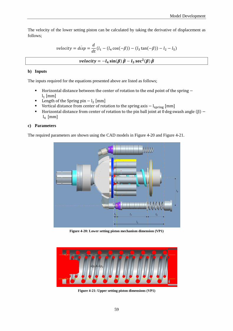
Model Development
59
The velocity of the lower setting piston can be calculated by taking the derivative of displacement as
follows;
b) Inputs
The inputs required for the equations presented above are listed as follows;
β
c) Parameters
The required parameters are shown using the CAD models in Figure 4-20 and Figure 4-21.
Figure 4-20: Lower setting piston mechanism dimension (VP1)
Figure 4-21: Upper setting piston dimensions (VP1)

Model Development
60
4.3.3.2.3 Servo Spring
a) Equations
The spring compression, spring force and the torque generated by the spring force acting on the swivel
inertia can be described using the equations presented below. Figure 4-22 and Figure 4-23 show the
trigonometry diagram used for formulating the equations for spring compression and spring torque
respectively.
Figure 4-22: Servo spring compression (VP1)
The spring length at a given swivel angle (β) is given by;
The spring force is given by;
Where is the e equivalent spring constant of the two parallelly placed springs and it is given by;
The torque on the swivel inertia due to servo spring is given by;
Moment arm is computed as follows;
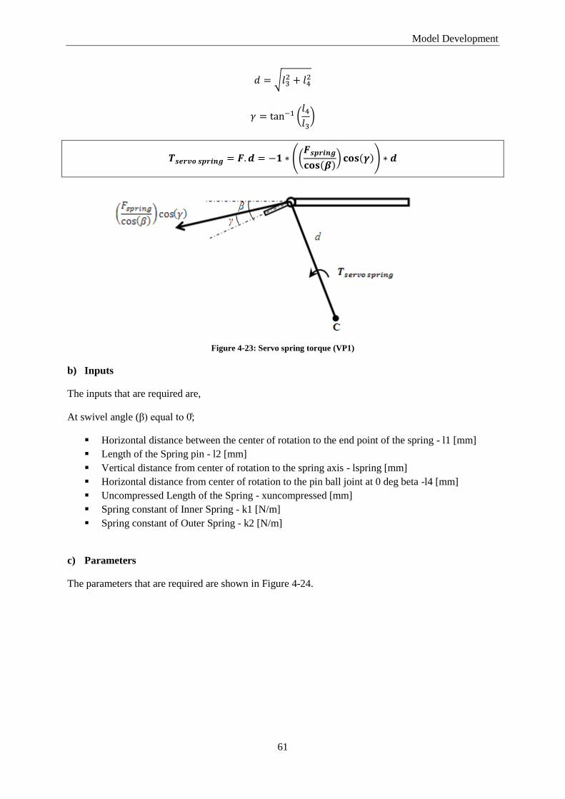
Model Development
61
Figure 4-23: Servo spring torque (VP1)
b) Inputs
The inputs that are required are,
At swivel angle (β) e ual to ;
Horizontal distance between the center of rotation to the end point of the spring - l1 [mm]
Length of the Spring pin - l2 [mm]
Vertical distance from center of rotation to the spring axis - lspring [mm]
Horizontal distance from center of rotation to the pin ball joint at 0 deg beta -l4 [mm]
Uncompressed Length of the Spring - xuncompressed [mm]
Spring constant of Inner Spring - k1 [N/m]
Spring constant of Outer Spring - k2 [N/m]
c) Parameters
The parameters that are required are shown in Figure 4-24.

Model Development
62
Figure 4-24: Servo spring dimension (VP1)
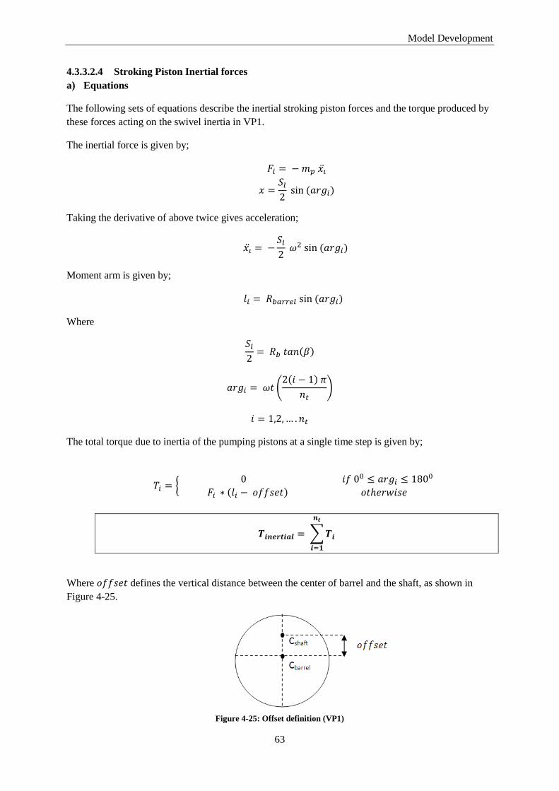
Model Development
63
4.3.3.2.4 Stroking Piston Inertial forces
a) Equations
The following sets of equations describe the inertial stroking piston forces and the torque produced by
these forces acting on the swivel inertia in VP1.
The inertial force is given by;
Taking the derivative of above twice gives acceleration;
Moment arm is given by;
Where
The total torque due to inertia of the pumping pistons at a single time step is given by;
Where defines the vertical distance between the center of barrel and the shaft, as shown in
Figure 4-25.
Figure 4-25: Offset definition (VP1)

Model Development
64
b) Inputs
The inputs required for the equations presented above are listed as follows;
Barrel Radius -Rb [mm]
Mass of One Piston - mp [kg]
Total Number of Pistons - nt [null]
Barrel Axis Offset - offset [mm]
Inertia of Barrel + Shaft [kgm^2]
c) Parameters
The parameters are shown in Figure 4-26.
Figure 4-26: Barrel radius (VP1)
4.3.3.2.5 Pressure Pulsation Torques
The pressure pulsation torque component used for VP1 simulation model is identical to the component
developed for PV plus. For diagram, inputs and equations please refer to section 4.3.2.2.4.
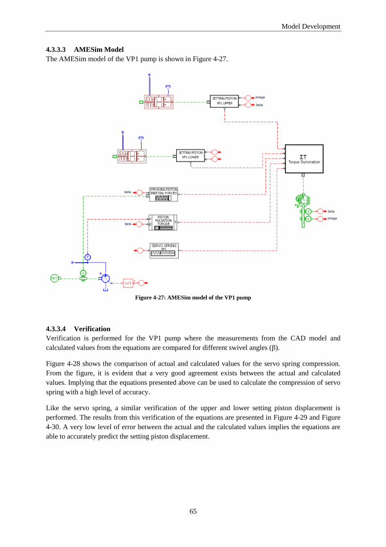
Model Development
65
4.3.3.3 AMESim Model
The AMESim model of the VP1 pump is shown in Figure 4-27.
Figure 4-27: AMESim model of the VP1 pump
4.3.3.4 Verification
Verification is performed for the VP1 pump where the measurements from the CAD model and
calculated values from the equations are compared for different swivel angles (β).
Figure 4-28 shows the comparison of actual and calculated values for the servo spring compression.
From the figure, it is evident that a very good agreement exists between the actual and calculated
values. Implying that the equations presented above can be used to calculate the compression of servo
spring with a high level of accuracy.
Like the servo spring, a similar verification of the upper and lower setting piston displacement is
performed. The results from this verification of the equations are presented in Figure 4-29 and Figure
4-30. A very low level of error between the actual and the calculated values implies the equations are
able to accurately predict the setting piston displacement.

Model Development
66
Figure 4-28: Comparison of servo spring compression (VP1)
Figure 4-29: Comparison of upper setting piston displacement (VP1)
Figure 4-30: Comparison of lower setting piston displacement (VP1)
-0,025
-0,02
-0,015
-0,01
-0,005
0
0
20
40
60
80
0 5 10 15 19,5
% E
rro
r
Co
mp
ress
ion [
mm
]
Swivel angle [degree]
Servo Spring
Actual
Calculated
% Error
-0,04
-0,03
-0,02
-0,01
0
0,01
0,02
0
5
10
15
20
25
30
0 5 10 15 19,5
% E
rro
r
Dis
pla
cem
ent
[mm
]
Swivel angle [degree]
Upper Setting Piston
Actual
Calculated
% Error
-0,04
-0,03
-0,02
-0,01
0
0,01
0,02
0
5
10
15
20
25
30
0 5 10 15 19,5
% E
rro
r
Dis
pla
cem
ent
[mm
]
Swivel angle [degree]
Lower Setting Piston
Actual
Calculated
% Error

Model Development
67
4.3.4 P2
4.3.4.1 Introduction
P2 is a variable inline axial piston pump. This pump series is available in four different sizes ranging
from 60 to 145 . For more information on P2 series pumps features and typical
applications refer to Parker Hannifin catalogue HY02-8001/UK.
4.3.4.2 Component (Mechanism) Equations
4.3.4.2.1 Setting Piston Mechanism
a) Equations
Setting Piston Displacement
As in the P2 pump the mechanism connecting the swivel inertia to the setting piston is identical to the
connection mechanism in PVplus, the displacement of the setting piston can be described by the same
equation. The displacement equation is given as follows;
However in P2, the setting piston is inclined at an angle, so the displacement needs to be
projected to get the actual displacement of the setting piston,
Figure 4-31: Setting piston displacement (P2)
From figure above we can see that;
As the setting piston is inclined, the Lact changes with the changing swivel angle. In order to calculate
Lact two points are taken to form a linear equation between Lact and swivel angle.
The general equation for a line is given by;

Model Development
68
The two points are,
(x1,y1): At β = , Lact = 75.83mm
(x2,y2): At β = , Lact = 82.87mm
Putting these values in the above equation and solving for Lact we get;
Setting Piston Velocity
Similarly the velocity of the setting piston can be calculated by the same equation used for PVplus.
Setting Piston Torque
The equation used to calculate the torque on the swivel inertia due to setting piston force also remains
the same as in PVplus.
As the mechanism in PV plus series pumps and P2 series pumps remain the same (i.e. chain link) the
equations governing the relation between the swivel angle and the setting piston displacement, swivel
velocity and setting piston velocity, setting piston force and torque on the swivel inertia remain the
same. The only major difference between the two setting piston deigns is that in P2 the setting piston
is inclined at an angle with the horizontal while in PV plus it is horizontal. This implies that we have
changing Lact value w.r.t swivel angle in P2 while in PV plus it remains constant.
b) Inputs
The inputs that are required are listed as follows;
Minimum Swivel Angle - b1 [deg]
Maximum Swivel Angle - b2 [deg]
Minimum Vertical length of Actuator - Lact1 [mm]
Maximum Vertical length of Actuator - Lact2 [mm]
Vertical distance between the chain link attachment point to swash plate and center of rotation
at swivel angle = 0 degree - dL2s [mm]
Horizontal distance between the center of rotation and the chain link connection point to the
swash plate at swivel angle = 0 degree - dcs [mm]
Radius of Swash Plate - Rswash [mm]
Length of the Chain Link - Lchain [mm]
Mass of Setting Piston and Chain link - m [kg]
Horizontal distance from center of rotation to the end point of the piston end stop - l1 [mm]
Length of the Piston - l2 [mm]
Angle of the piston to the center axis of the pump - alpha [deg]

Model Development
69
c) Parameters
The parameters that are required are shown using the Figure 4-32, Figure 4-33, Figure 4-34 and Figure
4-35.
Figure 4-32: Setting piston mechanism dimension (P2)
Figure 4-33: Setting piston mechanism dimension (P2)
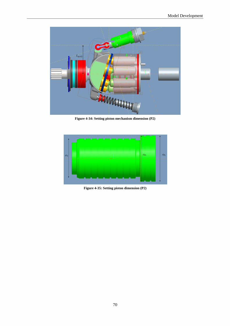
Model Development
70
Figure 4-34: Setting piston mechanism dimension (P2)
Figure 4-35: Setting piston dimension (P2)

Model Development
71
4.3.4.2.2 Servo spring
a) Equations
The spring compression, spring force and the torque generated by the spring force acting on the swivel
inertia can be described using the equations presented below. Figure 4-22 and Figure 4-37Figure 4-23
show the trigonometry diagrams used for formulating the equations for spring compression and spring
torque respectively.
Figure 4-36: Servo spring compression (P2)
The compression or spring length at a given swivel angle (β) is given by;
The force exerted by the servo spring due to its compression is given by;
Torque on the swivel inertia due to spring force is calculated as follows;

Model Development
72
Figure 4-37: Servo spring torque (P2)
b) Inputs
The following inputs are required.
Horizontal distance between the center of rotation and end point of the spring - l1 [mm]
Vertical distance between the center of rotation and spring axis - (lspring) l3 [mm]
Horizontal distance from center of rotation to the ball joint at swivel angle = 0 degree - l4
[mm]
Geometrical Angle of the Spring to the central axis of the pump - alpha [deg]
Uncompressed Length of the Spring -xuncompressed [mm]
Spring Constant - k [N/m]
c) Parameters
The parameters that are used are shown in Figure 4-38.
Figure 4-38: Servo spring dimensions (P2)

Model Development
73
4.3.4.2.3 Stroking Pistons Inertial Forces
Same pumping groups are used in PV plus and P2 series pumps. In both the cases these pumping
groups is held in place with help of part called the retainer ring. This retainer ring is directly fastened
to the swash plate.
Therefore the exact same equations and submodel developed for torque acting on the swivel inertia
due to inertia of the pumping group in PV plus can be used for P2 series pumps as well. Refer to
section 4.3.2.2.3 for equations, diagrams, inputs and parameters.
4.3.4.2.4 Piston Pulsation Torque
The pressure pulsation torque component used for P2 simulation model is identical to the component
developed for PV plus. For diagram, inputs and equations please refer to section 4.3.2.2.4.
4.3.4.3 AMESim Model
The AMESim model of the P2 pump is shown in the figure below;
Figure 4-39: AMESim model of the P2 pump
4.3.4.4 Verification
The verification process for the P2 pump equations include comparison of servo spring compression,
setting piston displacement and chain link angle values obtained by the equations presented above
with the CAD model measurements. The results are summarized in the Figure 4-40, Figure 4-41 and
Figure 4-42. A good agreement between the actual and the calculated values can be observed in these
figures.
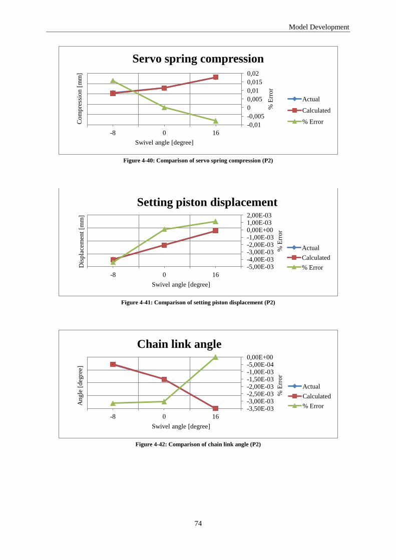
Model Development
74
Figure 4-40: Comparison of servo spring compression (P2)
Figure 4-41: Comparison of setting piston displacement (P2)
Figure 4-42: Comparison of chain link angle (P2)
-0,01
-0,005
0
0,005
0,01
0,015
0,02
0
20
40
60
80
100
-8 0 16
% E
rro
r
Co
mp
ress
ion [
mm
]
Swivel angle [degree]
Servo spring compression
Actual
Calculated
% Error
-5,00E-03 -4,00E-03 -3,00E-03 -2,00E-03 -1,00E-03 0,00E+00 1,00E-03 2,00E-03
-40
-30
-20
-10
0
-8 0 16 %
Err
or
Dis
pla
cem
ent
[mm
]
Swivel angle [degree]
Setting piston displacement
Actual
Calculated
% Error
-3,50E-03 -3,00E-03 -2,50E-03 -2,00E-03 -1,50E-03 -1,00E-03 -5,00E-04 0,00E+00
0
10
20
30
40
-8 0 16
% E
rro
r
Angle
[d
egre
e]
Swivel angle [degree]
Chain link angle
Actual
Calculated
% Error

Model Development
75
4.4 Bent Axis Motors
The following three machine series of bent axis design are studied.
1. C24
2. V14
3. V12
4.4.1 C24
4.4.1.1 Introduction
C24 is a bent-axis pump-motor. As it can act both as a pump and a motor it is used to recover or
regenerate energy in various applications. The size of the C24 that is modeled is C24-195
(195 ).
4.4.1.2 Component (Mechanism) Equations
4.4.1.2.1 Setting Piston Mechanism
a) Equations
The forces in the two setting pistons due to pressure inside the setting piston chamber can be split into
two forces as shown in the Figure 4-43. In the figure point C is the center of rotation for the swivel
inertia. This point also serves as the origin for the coordinate system.
Figure 4-43: Setting piston forces (C24)
Figure 4-44 defines the naming convention for the setting pistons. So looking at the top view as shown
in the figure the setting piston to the right is referred to as ‘setting piston A’ while the setting piston to
the left is referred to as ‘setting piston B’.
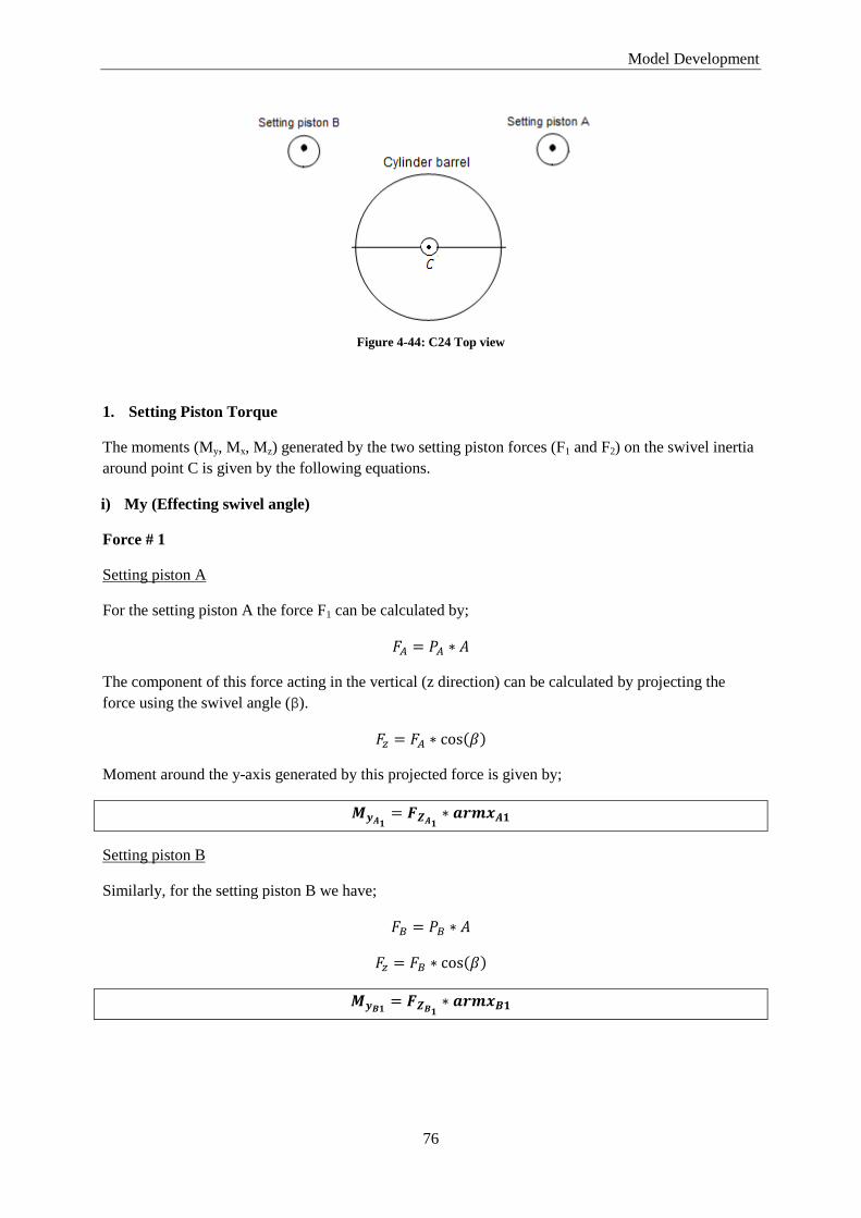
Model Development
76
Figure 4-44: C24 Top view
1. Setting Piston Torque
The moments (My, Mx, Mz) generated by the two setting piston forces (F1 and F2) on the swivel inertia
around point C is given by the following equations.
i) My (Effecting swivel angle)
Force # 1
Setting piston A
For the setting piston A the force F1 can be calculated by;
The component of this force acting in the vertical (z direction) can be calculated by projecting the
force using the swivel angle (β).
Moment around the y-axis generated by this projected force is given by;
Setting piston B
Similarly, for the setting piston B we have;

Model Development
77
The moment arms change as the swivel angle (β) changes. These moment arms ( and )
can be calculated as follows;
The distance r as shown in Figure 4-45 is defined by the following equation. In this equation the
and are defined as vertical and horizontal distances
from the center of rotation C to the top of the setting piston chamber respectively at swivel angle .
The moment arms for the two setting pistons are;
Figure 4-45: Moment arm armx_A1
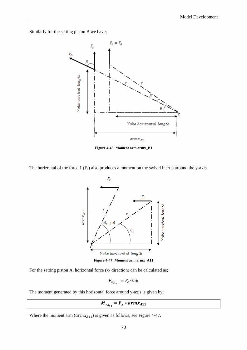
Model Development
78
Similarly for the setting piston B we have;
Figure 4-46: Moment arm armx_B1
The horizontal of the force 1 (F1) also produces a moment on the swivel inertia around the y-axis.
Figure 4-47: Moment arm armx_A11
For the setting piston A, horizontal force (x- direction) can be calculated as;
The moment generated by this horizontal force around y-axis is given by;
Where the moment arm ( ) is given as follows, see Figure 4-47.
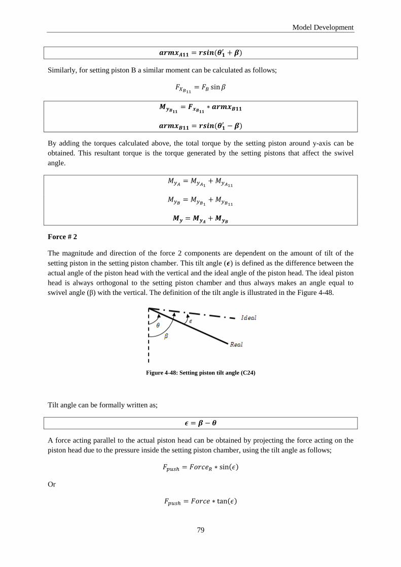
Model Development
79
Similarly, for setting piston B a similar moment can be calculated as follows;
By adding the torques calculated above, the total torque by the setting piston around y-axis can be
obtained. This resultant torque is the torque generated by the setting pistons that affect the swivel
angle.
Force # 2
The magnitude and direction of the force 2 components are dependent on the amount of tilt of the
setting piston in the setting piston chamber. This tilt angle ( ) is defined as the difference between the
actual angle of the piston head with the vertical and the ideal angle of the piston head. The ideal piston
head is always orthogonal to the setting piston chamber and thus always makes an angle equal to
swivel angle (β) with the vertical. The definition of the tilt angle is illustrated in the Figure 4-48.
Figure 4-48: Setting piston tilt angle (C24)
Tilt angle can be formally written as;
A force acting parallel to the actual piston head can be obtained by projecting the force acting on the
piston head due to the pressure inside the setting piston chamber, using the tilt angle as follows;
Or

Model Development
80
This force also produces a moment on the swivel inertia around y-axis (i.e. a moment that
affects the swivel angle of the machine). This moment produced by the two setting pistons is
illustrated in Figure 4-49.
Figure 4-49: Moment due to tilt forces affecting swivel angle (C24)
This moment can be calculated as follows;
The magnitude of the tilt angle is small ( ), thus the magnitude of tilt forces is also
small. Consequently when comparing the moments that affect the swivel angle, the moments produced
by the tilt forces are almost insignificant as compared to moments produced by other forces. Due to
this, the moment produced by the tilt forces is not included in the simulation model.

Model Development
81
ii) Mx (Effecting friction)
Some components of the setting piston force produce a moment around the x-axis. This moment will
tend to push one side of the yoke into the yoke bearing, thus contributing to an increased friction
between the yoke and the yoke bearing. Here the equations showing moment generated by the setting
piston forces in the x-axis are presented. While the impact of this moment on the friction coefficients
is not given as it is beyond the scope of the thesis work. Moreover, in the simulation model the
moment Mx is presented only as additional information for the user and is not used to calculate any
other parameter.
Force # 1
The contribution of the force F1 towards moment Mx can be calculated using the following set of
equations.
Setting piston A
Figure 4-50: Moments M_x_A_1 and M_x_B_1
For setting piston A, the component of the force F1 in the vertical (z-direction) can be written as;
The moment generated by this force is given by;
Where the moment arm is the horizontal distance between the center of rotation point C and the top of
the setting piston chamber. This moment arm remains constant.
Setting piston B
Similarly for setting piston B, the moment around x-axis can be written as follows;

Model Development
82
Both
do not change their direction and always support each other in trying to push the
upper part of the yoke (according to Figure 4-50) into the yoke bearing.
Force # 2
The contribution of the force F2 towards moment Mx can be calculated using the following set of
equations.
Figure 4-51: Moment M_x_A_2 and M_x_B_2
Setting piston A
The component of F2 in the vertical (- z-direction) can be written as follows;
The moment generated by this force about x-axis is given by;
Where the moment arm is the same as in the previous case and is given by;
Setting piston B
Similarly the corresponding moment can be calculated as follows;
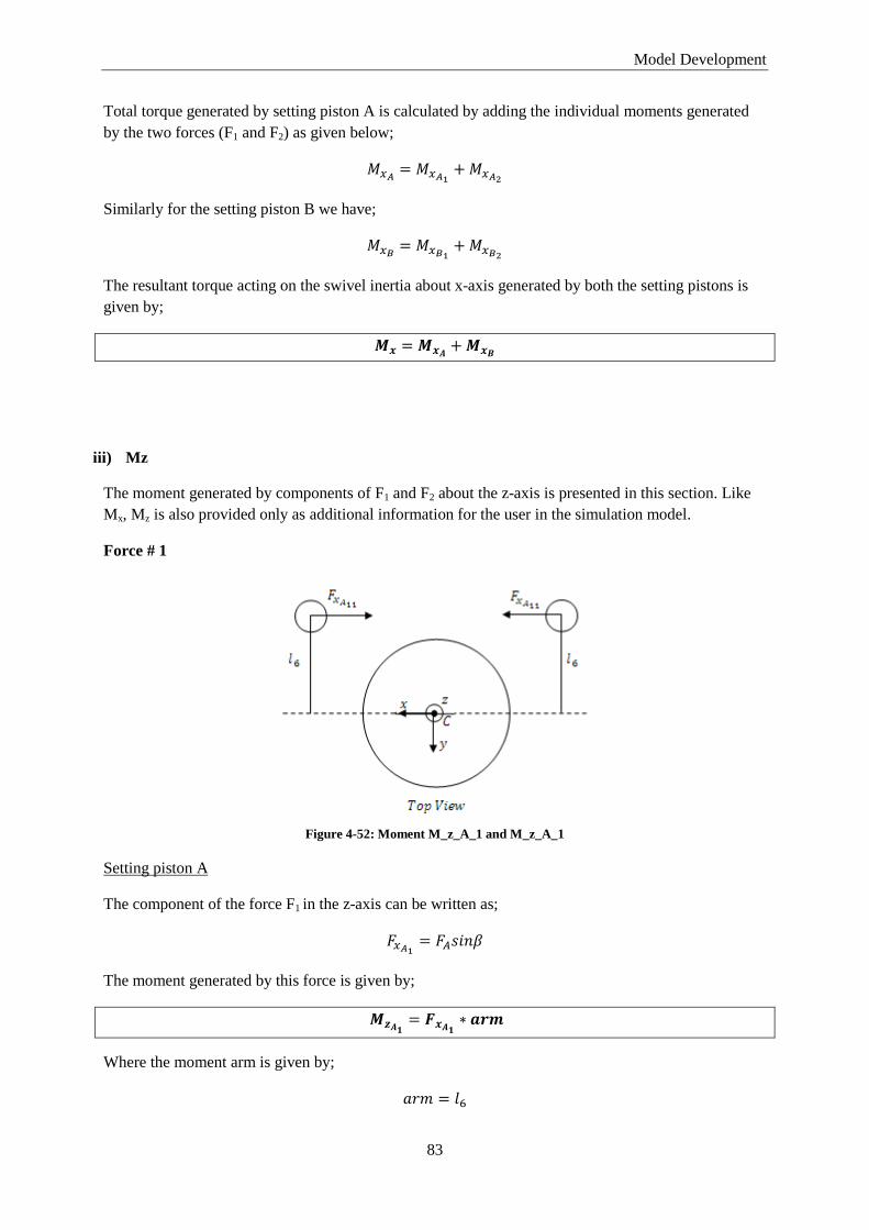
Model Development
83
Total torque generated by setting piston A is calculated by adding the individual moments generated
by the two forces (F1 and F2) as given below;
Similarly for the setting piston B we have;
The resultant torque acting on the swivel inertia about x-axis generated by both the setting pistons is
given by;
iii) Mz
The moment generated by components of F1 and F2 about the z-axis is presented in this section. Like
Mx, Mz is also provided only as additional information for the user in the simulation model.
Force # 1
Figure 4-52: Moment M_z_A_1 and M_z_A_1
Setting piston A
The component of the force F1 in the z-axis can be written as;
The moment generated by this force is given by;
Where the moment arm is given by;

Model Development
84
Setting piston B
Similarly for the setting piston B, we have;
Force # 2
Setting piston A
By projecting the force F1 using angle , the component of force F2 in the x-direction can be written as
follows;
The moment generated by about z-axis is given by;
While the moment arm is given by;
Setting piston B
Similarly for setting piston we have;

Model Development
85
The total torque generated by the setting piston about z-axis is given by;
2. Setting Piston Displacement
The equations describing the relationship between the swivel angle (β) and the setting piston
displacement are presented in this section.
C24 Angle Convention
Before the description of the equations to calculate the setting piston displacement for a given swivel
angle, it is necessary to present the convention for the direction of the swivel angle (β) and angle of the
setting piston with the vertical (θ) used. Figure 4-53 illustrates this convention.
Figure 4-53: C24 Angle direction convention (Front view)
Setting piston A
Following set of equations can be used to calculate the angle of the setting piston with the vertical;
Setting Piston Angle

Model Development
86
Figure 4-54: Setting piston angle θ (C24)
Setting Piston Displacement
For a given swivel angle (β) the corresponding displacement of the setting piston ( ) can be
calculated as follows;

Model Development
87
Setting Piston Velocity
The velocity of the setting piston can be given by;
Where is given by;
Setting piston B
Similarly for setting piston B, the angle of the setting piston with the vertical is given as follows;
Setting Piston Angle
Setting Piston Displacement
The displacement of the setting piston is given by;

Model Development
88
Setting Piston Velocity
The velocity of the setting piston is given by;
Where is given by;
b) Inputs
The inputs required by the simulation model to calculate the setting piston torque, displacement and
velocity are listed as follows;
Setting Piston A
For the setting piston A the required inputs are;
Length of the piston from center of ball joint to piston head center - l1 [mm]
Radius of piston ring - l2 [mm]
Horizontal distance between center of rotation and setting piston chamber at swivel angle = 0
degree - l3 [mm]
Horizontal distance between center of rotation and center of setting piston ball joint at swivel
angle = 0 degree - l4 [mm]
Vertical distance between center of rotation and center of setting piston ball joint at swivel
angle = 0 degree - l5 [mm]
Side view distance between center of rotation and center of setting piston ball joint - l6 [mm]
Distance between center of rotation and center of setting piston head at maximum swivel
angle - R1 [mm]
Setting piston stroke - xmin [mm]
a - Yoke vertical length [mm]
b - Yoke horizontal length [mm]
Setting Piston B
For the setting piston B the required inputs are;
Length of the piston from center of ball joint to piston head center - l1 [mm]
Radius of piston ring - l2 [mm]
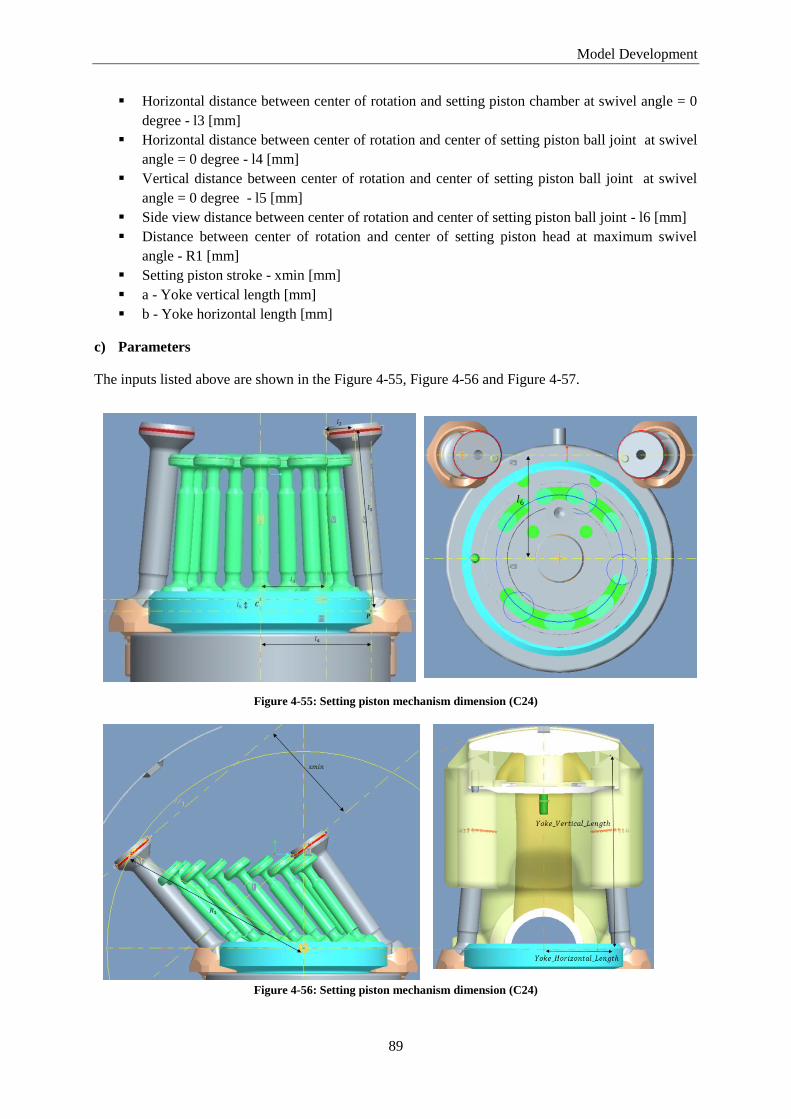
Model Development
89
Horizontal distance between center of rotation and setting piston chamber at swivel angle = 0
degree - l3 [mm]
Horizontal distance between center of rotation and center of setting piston ball joint at swivel
angle = 0 degree - l4 [mm]
Vertical distance between center of rotation and center of setting piston ball joint at swivel
angle = 0 degree - l5 [mm]
Side view distance between center of rotation and center of setting piston ball joint - l6 [mm]
Distance between center of rotation and center of setting piston head at maximum swivel
angle - R1 [mm]
Setting piston stroke - xmin [mm]
a - Yoke vertical length [mm]
b - Yoke horizontal length [mm]
c) Parameters
The inputs listed above are shown in the Figure 4-55, Figure 4-56 and Figure 4-57.
Figure 4-55: Setting piston mechanism dimension (C24)
Figure 4-56: Setting piston mechanism dimension (C24)
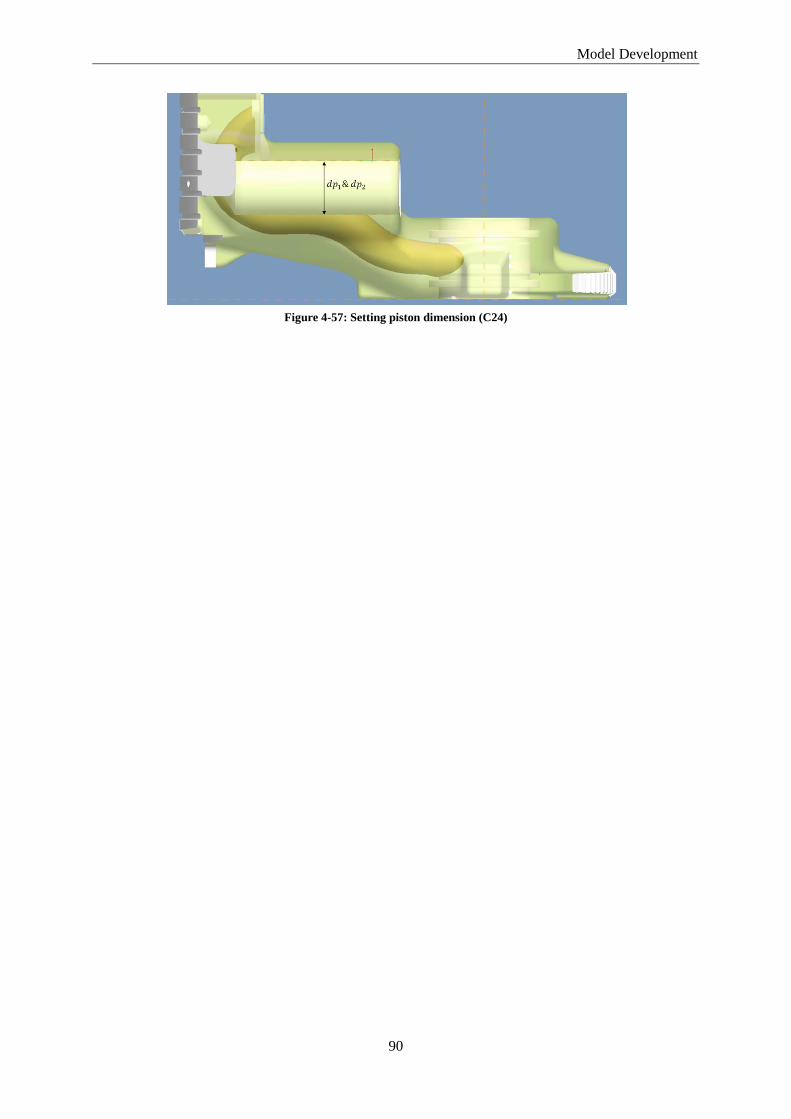
Model Development
90
Figure 4-57: Setting piston dimension (C24)

Model Development
91
4.4.1.2.2 Stroking Piston Inertial Forces
Mathematical equations describing the inertial forces generated by the reciprocating motion of the
stroking pistons are presented in this section. Moreover the equations describing the torque generated
by these inertial forces on the swivel inertia are also presented here.
a) Equations
The base of a stroking piston (i.e. ball socket) rotates in a circle as shown in Figure 4-58.
Figure 4-58: Rotation of a stroking piston
However the head of a stroking piston does not follow a completely circular trajectory. Instead it
moves in an elliptical shape as shown in Figure 4-59. The shape and size of this ellipse is dependent
on the swivel angle (β). or a swivel angle this ellipse takes the shape of a circle and elongates as the
swivel angle increases.
Figure 4-59: Elliptical movement of a stroking piston head
The semi-major and semi-minor axes of the ellipse along with other parameters are defined in the
Figure 4-60.

Model Development
92
Figure 4-60: Ellipse parameter definition
Due to its elliptical trajectory, the piston head with reference to its base moves both vertically and
horizontally. Moreover, the relation of the vertical and horizontal movement of the piston head is not
linear with the angle of rotation of the piston. In other words the piston head accelerates and
decelerates during these movements. Inertial forces arise due to these accelerations. Therefore a
vertical acceleration of the piston head gives rise to a vertical inertial force while a horizontal force is
generated due to a horizontal acceleration, as shown in Figure 4-61.
Figure 4-61: Horizontal and vertical (a) acceleration (b) inertial force
Figure 4-62: Projection of lp (length of piston)
From Figure 4-60 and Figure 4-62 we can write that;

Model Development
93
The horizontal distance of the piston head with reference to its base at angle of rotation of the piston
( ) is given by;
Furthermore;

Model Development
94
The horizontal distance of the piston head with reference to its base at 1 angle of rotation of the
piston ( ) is given by;
The horizontal distance between the piston head and its base is maximum at and 1 angle of
rotation ( ) of the piston as shown in Figure 4-63. Moreover this distance is ero at and 2 . The
movement of the piston head follows a cosine function. The hori ontal distance at and 1 can be
used to calculate the amplitude of this cosine function.
Figure 4-63: Horizontal movement of the piston head (Front view)
The amplitude is given by;
The horizontal displacement is given by;
The vertical displacement is given by;
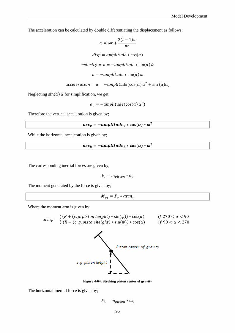
Model Development
95
The acceleration can be calculated by double differentiating the displacement as follows;
Neglecting for simplification, we get
Therefore the vertical acceleration is given by;
While the horizontal acceleration is given by;
The corresponding inertial forces are given by;
The moment generated by the force is given by;
Where the moment arm is given by;
Figure 4-64: Stroking piston center of gravity
The horizontal inertial force is given by;

Model Development
96
The moment generated by the force is given by;
Where the moment is given by;
The total torque due to stroking pistons is obtained by adding all the torques generated by individual
pistons.
b) Inputs
The inputs that are required are listed as follows;
Mass of piston - mp [kg]
Number of Pistons - nt [null]
Length of the Pumping Piston - lp [mm]
Radius of the circle where the pistons are mounted - R [mm]
Ellipse radius of the pistons at beta = 0 or barrel radius of the piston - Radius1 [mm]
Center of gravity of piston (w.r.t piston base, in the direction of piston axis) - cgheight [mm]
c) Parameters
The required inputs are shown in the figure below,
Figure 4-65: C24 - Radius of circle where pistons are mounted (C24)

Model Development
97
4.4.1.2.3 Piston Pulsation Torque
a) Equations
The equation that is used is given by,
b) Inputs
The inputs that are required are,
Name of Force file
Name of y-coordinate file
Output Equation
Motor Equation
c) Diagram
The piston pulsation torque component is built using the standard AMESim components as shown in
the Figure 4-12.
4.4.1.3 AMESim Model
The AMESim model of the C24 pump-motor is shown in the figure below,
Figure 4-66: AMESim model of the C24 pump-motor
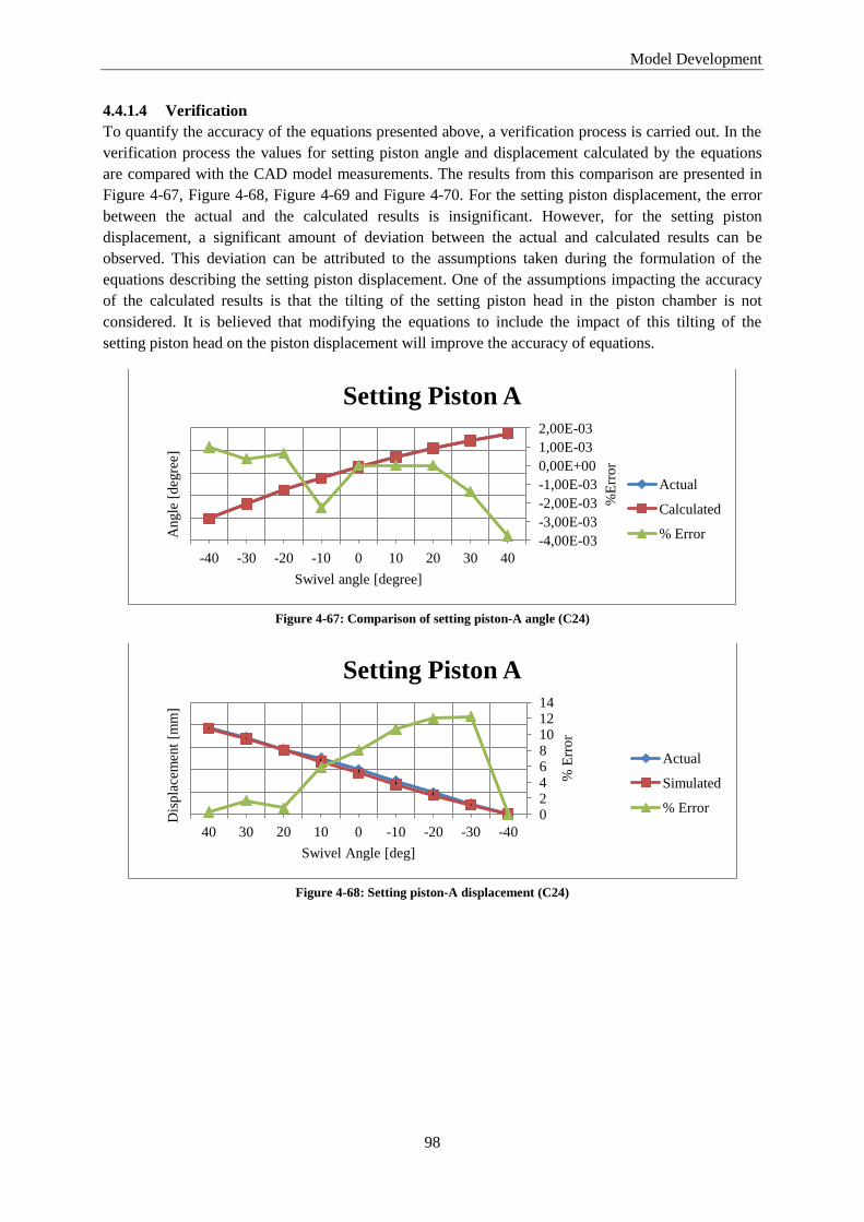
Model Development
98
4.4.1.4 Verification
To quantify the accuracy of the equations presented above, a verification process is carried out. In the
verification process the values for setting piston angle and displacement calculated by the equations
are compared with the CAD model measurements. The results from this comparison are presented in
Figure 4-67, Figure 4-68, Figure 4-69 and Figure 4-70. For the setting piston displacement, the error
between the actual and the calculated results is insignificant. However, for the setting piston
displacement, a significant amount of deviation between the actual and calculated results can be
observed. This deviation can be attributed to the assumptions taken during the formulation of the
equations describing the setting piston displacement. One of the assumptions impacting the accuracy
of the calculated results is that the tilting of the setting piston head in the piston chamber is not
considered. It is believed that modifying the equations to include the impact of this tilting of the
setting piston head on the piston displacement will improve the accuracy of equations.
Figure 4-67: Comparison of setting piston-A angle (C24)
Figure 4-68: Setting piston-A displacement (C24)
-4,00E-03
-3,00E-03
-2,00E-03
-1,00E-03
0,00E+00
1,00E-03
2,00E-03
-60
-40
-20
0
20
40
-40 -30 -20 -10 0 10 20 30 40
%E
rro
r
Angle
[d
egre
e]
Swivel angle [degree]
Setting Piston A
Actual
Calculated
% Error
0 2 4 6 8 10 12 14
0
20
40
60
80
100
40 30 20 10 0 -10 -20 -30 -40
% E
rro
r
Dis
pla
cem
ent
[mm
]
Swivel Angle [deg]
Setting Piston A
Actual
Simulated
% Error
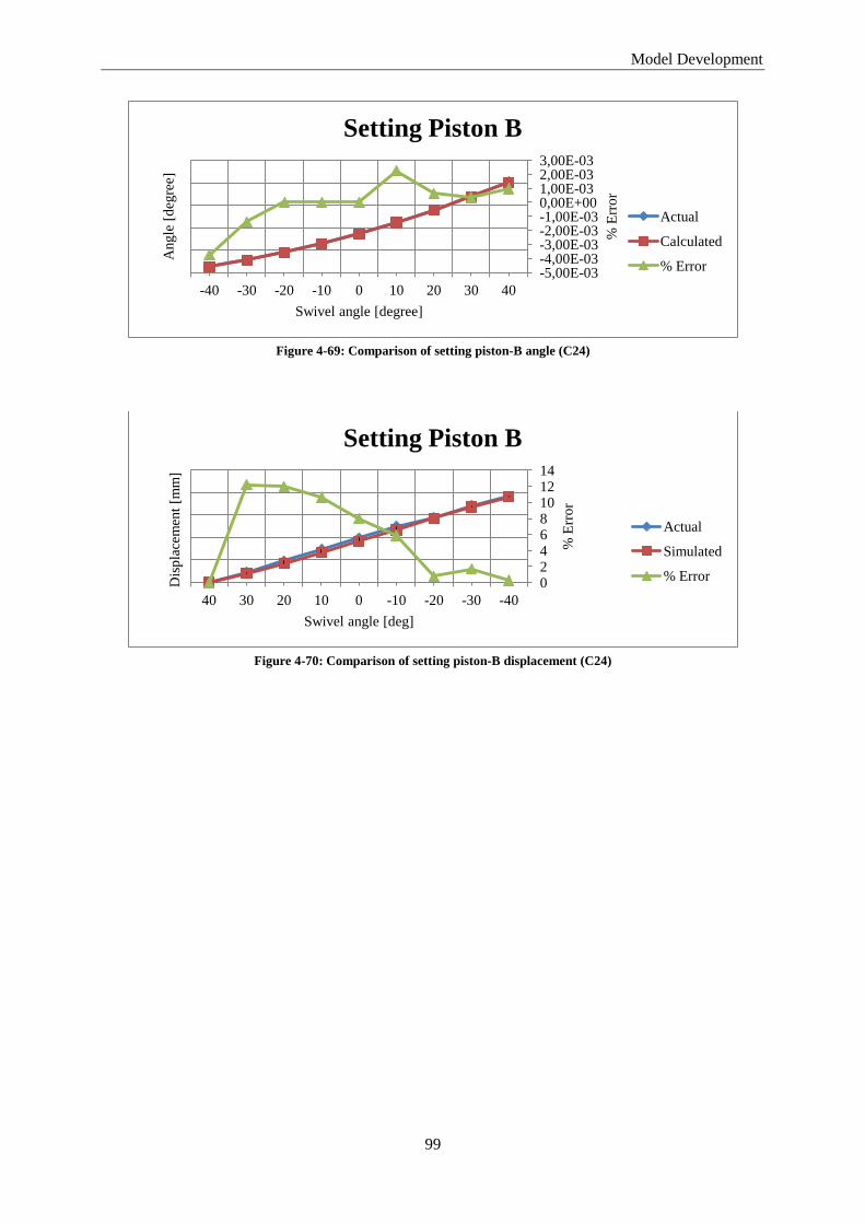
Model Development
99
Figure 4-69: Comparison of setting piston-B angle (C24)
Figure 4-70: Comparison of setting piston-B displacement (C24)
-5,00E-03 -4,00E-03 -3,00E-03 -2,00E-03 -1,00E-03 0,00E+00 1,00E-03 2,00E-03 3,00E-03
-40
-20
0
20
40
60
-40 -30 -20 -10 0 10 20 30 40
% E
rro
r
Angle
[d
egre
e]
Swivel angle [degree]
Setting Piston B
Actual
Calculated
% Error
0 2 4 6 8 10 12 14
0
20
40
60
80
100
40 30 20 10 0 -10 -20 -30 -40
% E
rro
r
Dis
pla
cem
ent
[mm
]
Swivel angle [deg]
Setting Piston B
Actual
Simulated
% Error

Model Development
100
4.4.2 V14
4.4.2.1 Introduction
V14 is a variable bent-axis motor. It is based on the Parker Hannifin V12 motor design. This motor is
designed for both open and closed circuit transmissions with focus on high performance machines.
The V14 motor is manufactured in two different sizes V14-110 (110 ) and 14-160
(160 ). Detail information about V14 motor can found in the Parker Hannifin catalogue
HY30-8223/UK.
4.4.2.2 Component (Mechanism) Equations
4.4.2.2.1 Setting Piston Mechanism
a) Equations
Setting Piston Torque
In V14, the setting piston is coincident with the horizontal (i.e. x-axis), therefore
Torque produced by around the center of rotation C is given by;
The moment arm is given by;
Figure 4-71: Setting piston torque (V14)

Model Development
101
Setting Piston Displacement
The displacement of the setting piston is given by,
Figure 4-72: Setting piston displacement (V14)
Setting Piston Velocity
Then the velocity of the setting piston is given by,
b) Inputs
The inputs that are required are,
Length of the Actuator in top view - lact [mm]
Length of the pin in top view - lpin [mm]
Setting Piston Displacement at minimum setting angle - xmin [mm]
Angle of the Setting Piston - thetas [deg]
c) Parameters
The required inputs are shown in Figure 4-73.

Model Development
102
Figure 4-73: Setting piston mechanism dimension (V14)
4.4.2.2.2 Stroking Piston Inertial Forces
The rotating group used in V14 motors is identical in design to the rotating group used in C24 pump
motor. Therefore the equations describing the inertial forces and the torque resulting from them in a
C24 machine are also applicable for V14.
4.4.2.2.3 Pressure Pulsation Torque
Like the inertial forces, component and equation used for the pressure pulsation forces in the V14
simulation model are the same as C24.For diagram, inputs and equations please refer to section
4.4.1.2.3.
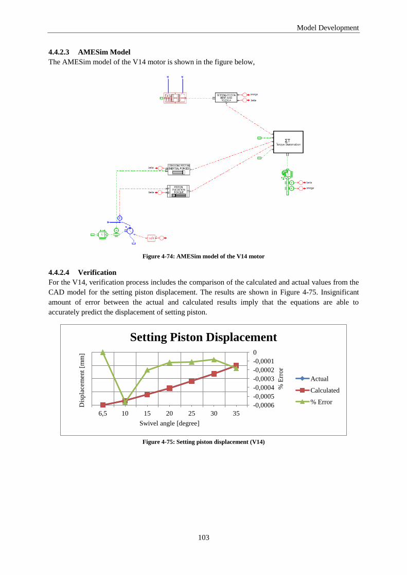
Model Development
103
4.4.2.3 AMESim Model
The AMESim model of the V14 motor is shown in the figure below,
Figure 4-74: AMESim model of the V14 motor
4.4.2.4 Verification
For the V14, verification process includes the comparison of the calculated and actual values from the
CAD model for the setting piston displacement. The results are shown in Figure 4-75. Insignificant
amount of error between the actual and calculated results imply that the equations are able to
accurately predict the displacement of setting piston.
Figure 4-75: Setting piston displacement (V14)
-0,0006
-0,0005
-0,0004
-0,0003
-0,0002
-0,0001
0
0
20
40
60
80
6,5 10 15 20 25 30 35
% E
rro
r
Dis
pla
cem
ent
[mm
]
Swivel angle [degree]
Setting Piston Displacement
Actual
Calculated
% Error

Model Development
104
4.4.3 V12
4.4.3.1 Introduction
V12 is a variable bent-axis motor. This motor is primarily used in mobile machinery. The V12 motor
is available in two sizes V12-60 (60 ) and V12-80 (80 ). Refer to Parker Hannifin
catalogue HY30-8223/UK for more information on the V12 motor.
4.4.3.2 Component (Mechanism) Equations
4.4.3.2.1 Setting Piston Mechanism
a) Equations
Setting Piston Torque
The force (F) produced by the setting piston can be resolved into its components;
Torque produced by around center of rotation C is given by;
The moment arm is given by;
Figure 4-76: Setting piston torque (V12)

Model Development
105
Setting Piston Displacement
For a certain swivel angle the setting piston displacement is given by;
Figure 4-77: Setting piston displacement (V12)
Setting Piston Velocity
The velocity of the setting piston is determined by differentiating the displacement equation;
b) Inputs
The inputs are defined as,
Length of the Actuator in top view - lact [mm]
Length of the pin in top view - lpin [mm]
Setting Piston Displacement at minimum setting angle - xmin [mm]
Angle of the Setting Piston - thetas [deg]
4.4.3.2.2 Stroking Piston Inertial Forces
The trigonometry and the equations are the same as described for the C24 pump-motor.
4.4.3.2.3 Piston Pulsation Torque
The pressure pulsation torque component used for V14 simulation model is identical to the component
developed for C24. For diagram, inputs and equations please refer to section 4.4.1.2.3.
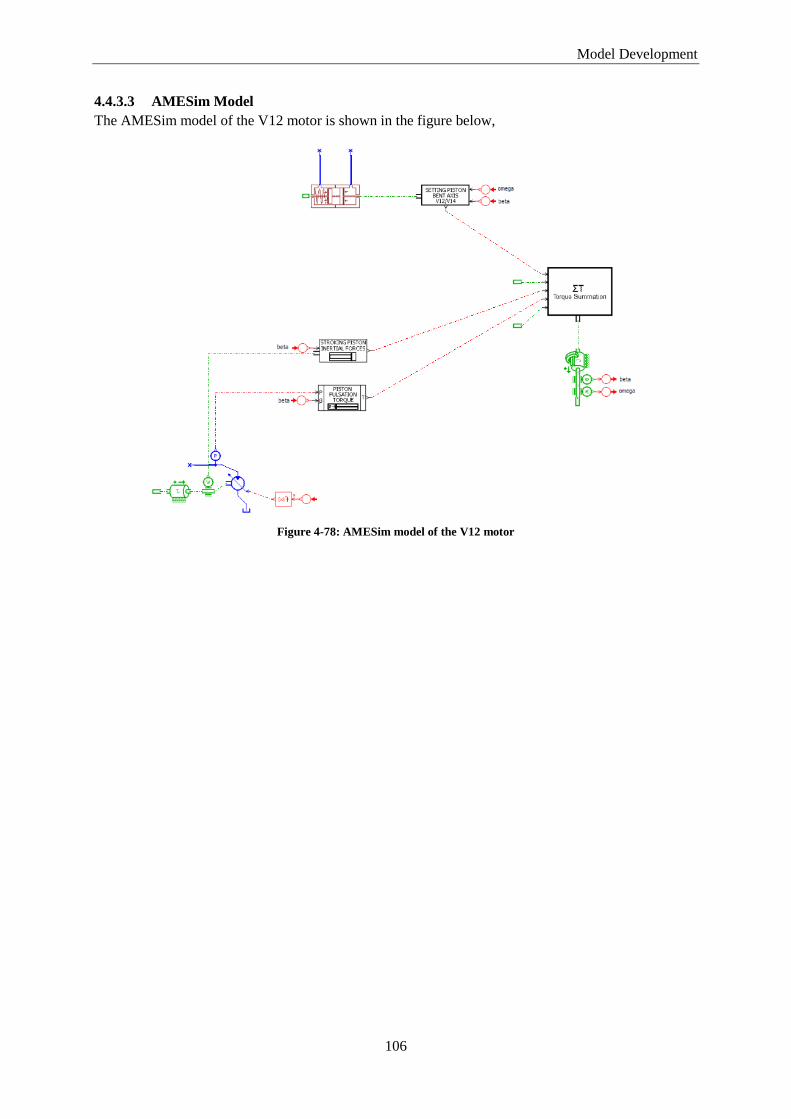
Model Development
106
4.4.3.3 AMESim Model
The AMESim model of the V12 motor is shown in the figure below,
Figure 4-78: AMESim model of the V12 motor
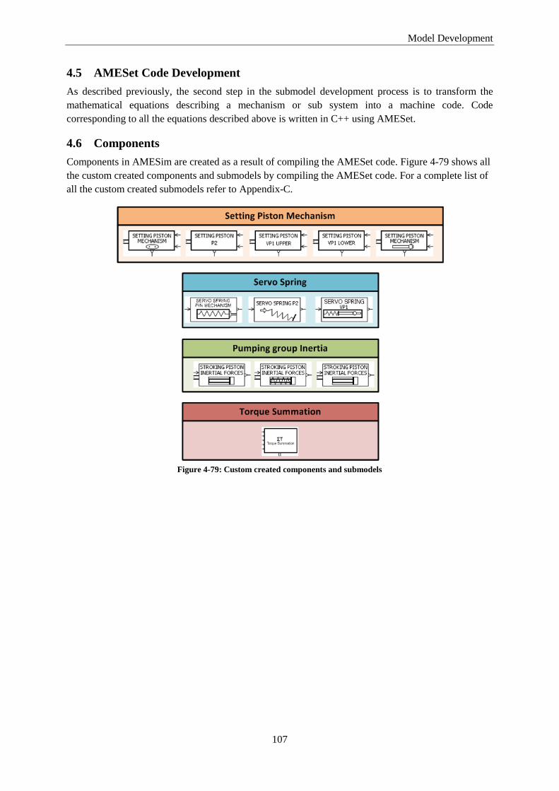
Model Development
107
4.5 AMESet Code Development
As described previously, the second step in the submodel development process is to transform the
mathematical equations describing a mechanism or sub system into a machine code. Code
corresponding to all the equations described above is written in C++ using AMESet.
4.6 Components
Components in AMESim are created as a result of compiling the AMESet code. Figure 4-79 shows all
the custom created components and submodels by compiling the AMESet code. For a complete list of
all the custom created submodels refer to Appendix-C.
Figure 4-79: Custom created components and submodels


5 Generic
Simulation Model
5.1 Generic Model
After the creation of components and its associated submodels, the generic simulation model of
hydraulic axial piston machines is developed. Figure 5-1 shows the generic simulation model. The
generic model contains all the components and submodels so that it is able to represent any pump or
motor under consideration. In the generic model, the setting piston mechanism, servo spring
mechanism, stroking piston inertial forces, piston pulsation forces and corresponding torques are
modeled. In the model standard AMESim components are used alongside with custom built
components and submodels. This generic simulation model is able to be transformed into a model
representing any of the six pumps/motors under consideration. Moreover, through parametric changes
in the generic simulation model it is able to represent any size of a pump/motor within the six
pump/motor series.
Figure 5-1: Generic simulation model for hydraulic axial piston machines
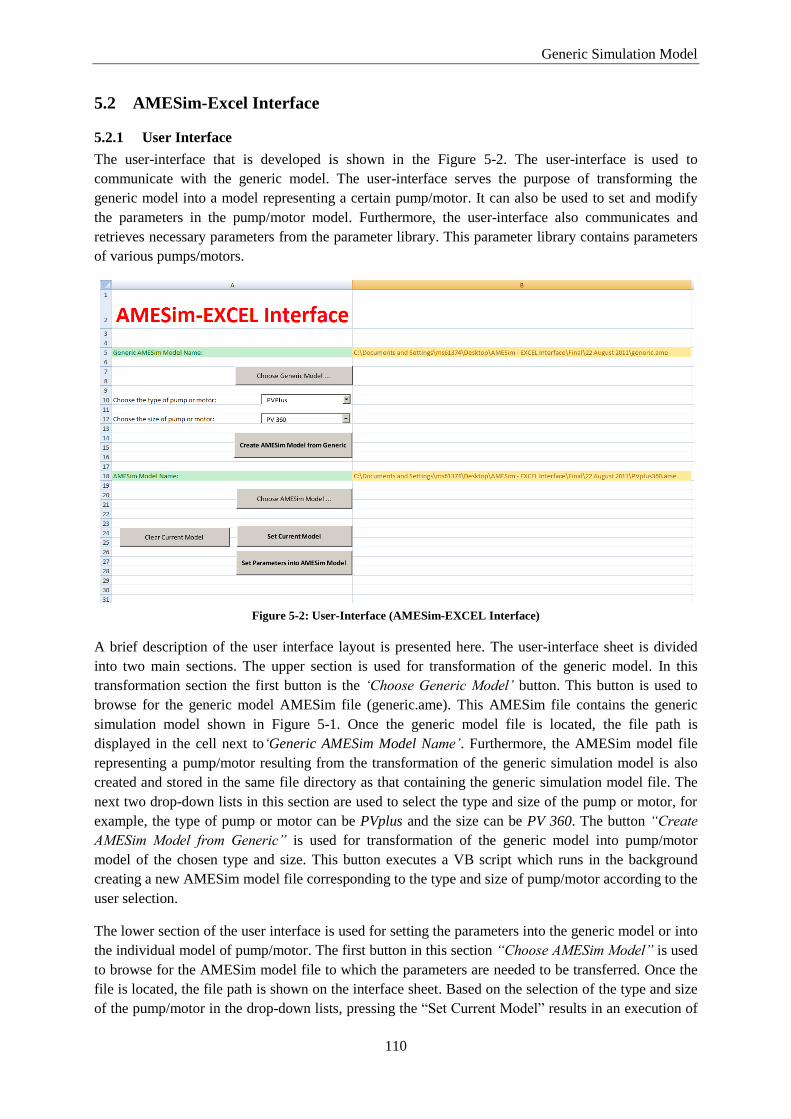
Generic Simulation Model
110
5.2 AMESim-Excel Interface
5.2.1 User Interface
The user-interface that is developed is shown in the Figure 5-2. The user-interface is used to
communicate with the generic model. The user-interface serves the purpose of transforming the
generic model into a model representing a certain pump/motor. It can also be used to set and modify
the parameters in the pump/motor model. Furthermore, the user-interface also communicates and
retrieves necessary parameters from the parameter library. This parameter library contains parameters
of various pumps/motors.
Figure 5-2: User-Interface (AMESim-EXCEL Interface)
A brief description of the user interface layout is presented here. The user-interface sheet is divided
into two main sections. The upper section is used for transformation of the generic model. In this
transformation section the first button is the ‘Choose Generic Model’ button. This button is used to
browse for the generic model AMESim file (generic.ame). This AMESim file contains the generic
simulation model shown in Figure 5-1. Once the generic model file is located, the file path is
displayed in the cell next to‘Generic AMESim Model Name’. Furthermore, the AMESim model file
representing a pump/motor resulting from the transformation of the generic simulation model is also
created and stored in the same file directory as that containing the generic simulation model file. The
next two drop-down lists in this section are used to select the type and size of the pump or motor, for
example, the type of pump or motor can be PVplus and the size can be PV 360. The button “Create
AMESim Model from Generic” is used for transformation of the generic model into pump/motor
model of the chosen type and size. This button executes a VB script which runs in the background
creating a new AMESim model file corresponding to the type and size of pump/motor according to the
user selection.
The lower section of the user interface is used for setting the parameters into the generic model or into
the individual model of pump/motor. The first button in this section “Choose AMESim Model” is used
to browse for the AMESim model file to which the parameters are needed to be transferred. Once the
file is located, the file path is shown on the interface sheet. Based on the selection of the type and size
of the pump/motor in the drop-down lists, pressing the “Set Current Model” results in an execution of

Generic Simulation Model
111
a VB script that transfers all the parameters of the selected pump/motor into the current model sheet.
In the current model sheet the parameters can then be modified by the user. The “Clear Current
Model” button is used to clear the contents of the current model sheet. Once all the necessary changes
to the parameters are made in the current model sheet, the parameters can be transferred to the
AMESim model file by pressing the “Set Parameters Into AMESim Model” button. Pressing this
button triggers a VB script, which runs in the background and transfers the parameters into appropriate
components and submodels in the AMESim model file thus updating it.
5.2.2 Parameter Library
The parameter library is a database of all the parameters that are required to model the pumps and
motors under consideration in this work. As an example, the parameter sheet for the PVplus 360 pump
is shown in the Figure 5-3.
Figure 5-3: Parameter Library: PVplus parameter sheet
As we can see from the figure that all the parameters are systematically placed in the parameter sheet
by grouping them into nine sections. The sections are Maximum and minimum swash angle, Setting
piston mechanism, Setting piston dimensions, Servo spring mechanism, Stroking piston inertial forces
mechanism, Other pump characteristics, Rotary load, Mechanical and volumetric efficiency, Piston
pulsation torque. The parameter values are taken from the CAD models, product catalogues and other
sources. The diagrams next to the parameters define the different parameters. Separate columns are
assigned to track the changes made in the parameter values. Individual parameter sheets are populated
for PVplus, VP1, P2, V12, V14 and C24.

Generic Simulation Model
112
5.2.3 Transformation of Generic model
The workflow followed to perform a transformation or a parametric change of the generic model is
shown in Figure 5-4. The user-interface is used to perform either of these operations on the generic
model.
Figure 5-4: Workflow followed by the user interface
5.2.3.1 AMESim API
In order to perform a transformation of the generic model, a Visual Basic script is written that utilizes
the AMESim Application Programming Interface (API). AMESim API consists of a set of functions
and classes that are used to communicate with AMESim. This API contains, for example functions for
addition and deletion of components and hydraulic lines, changing of submodels, rotating and flipping
the components, and setting the parameter value of components and submodels etc. For further
information on the AMESim API refer to AMESim help [12].
5.2.3.2 Parametric Change
In order to perform a parametric change in the generic simulation model, firstly, the type and size of
the pump or motor model is selected. Secondly, the AMESim file is browsed for which the parameter
values are needed to be changed. Once this is done, the parameters can be transferred to the current
model sheet by using the set current model button. A visual basic script runs in the background when
this button is pressed, copying all the contents of the selected pump/motor sheet and transferring it to
the current model sheet. The user has then the ability to change the parameter values in the current
model sheet. Once the user is satisfied with the parameter values to transfer to the AMESim model,

Generic Simulation Model
113
the set parameters to AMESim button is pressed. This button runs a Visual Basic script that utilizes the
AMESim API file to open the simulation model in the background, and set parameter values into all
the components of the model. Once the parameter values are transferred into the simulation model, the
model file is saved and closed.
5.2.3.3 Transformation to a Pump/Motor Model
In order to perform a transformation of the generic model into a certain pump or motor model, firstly,
the type and size of the pump or motor is selected in the user-interface. After this selection, the create
AMESim model from generic button is pressed. This button triggers a Visual Basic code which runs in
the background utilizing the AMESim API in order to transform the generic model into the required
pump/motor file. Firstly this code opens the generic model in AMESim followed by the deletion of
components in the generic model file that are not required. After the deletion of components, if
required, components are added in the simulation model. The VB code then links these components
automatically using hydraulic and signal lines. After all the components are linked, the code then
changes the submodels of the components to submodel describing the required pump/motor. The code
then saves the generic model as a new AMESim model file (.ame file). The final step is to close the
generic model and AMESim API.
A transformation of the generic simulation model into a PVplus 360 model is illustrated in the Figure
5-5. In the figure, it can be seen that some components are deleted and submodels are changed to
create a PVplus 360 simulation model.
Figure 5-5: Transformation to pump/motor model

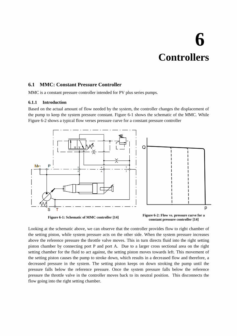
6 Controllers
6.1 MMC: Constant Pressure Controller
MMC is a constant pressure controller intended for PV plus series pumps.
6.1.1 Introduction
Based on the actual amount of flow needed by the system, the controller changes the displacement of
the pump to keep the system pressure constant. Figure 6-1 shows the schematic of the MMC. While
Figure 6-2 shows a typical flow verses pressure curve for a constant pressure controller
Figure 6-1: Schematic of MMC controller [14] Figure 6-2: Flow vs. pressure curve for a
constant pressure controller [14]
Looking at the schematic above, we can observe that the controller provides flow to right chamber of
the setting piston, while system pressure acts on the other side. When the system pressure increases
above the reference pressure the throttle valve moves. This in turn directs fluid into the right setting
piston chamber by connecting port P and port A. Due to a larger cross sectional area on the right
setting chamber for the fluid to act against, the setting piston moves towards left. This movement of
the setting piston causes the pump to stroke down, which results in a decreased flow and therefore, a
decreased pressure in the system. The setting piston keeps on down stroking the pump until the
pressure falls below the reference pressure. Once the system pressure falls below the reference
pressure the throttle valve in the controller moves back to its neutral position. This disconnects the
flow going into the right setting chamber.
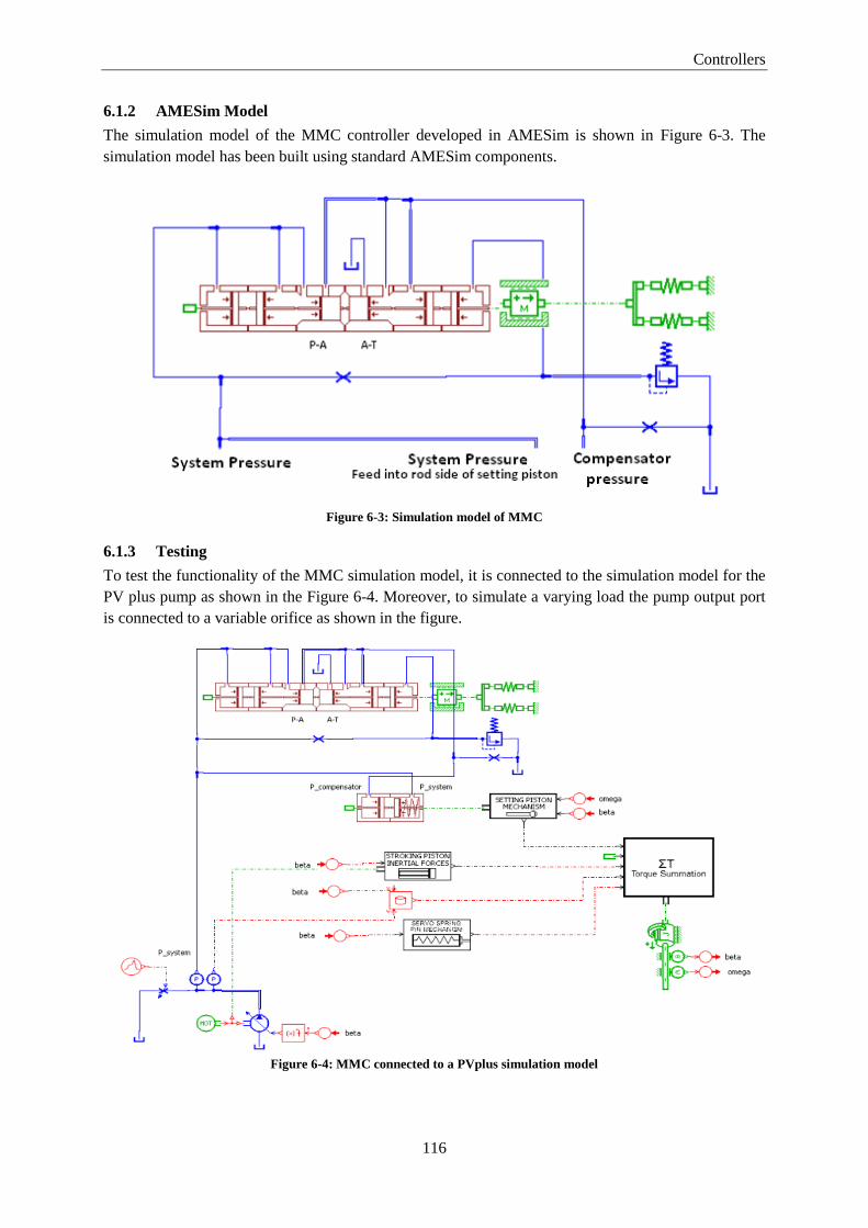
Controllers
116
6.1.2 AMESim Model
The simulation model of the MMC controller developed in AMESim is shown in Figure 6-3. The
simulation model has been built using standard AMESim components.
Figure 6-3: Simulation model of MMC
6.1.3 Testing
To test the functionality of the MMC simulation model, it is connected to the simulation model for the
PV plus pump as shown in the Figure 6-4. Moreover, to simulate a varying load the pump output port
is connected to a variable orifice as shown in the figure.
Figure 6-4: MMC connected to a PVplus simulation model

Controllers
117
To study the overall performance of the constant pressure controller, the load in the system is changed
by changing the variable orifice area. We can see in Figure 6-5 that until the system pressure remains
below the reference pressure the pump is allowed to deliver the required flow. However, once the
system pressure goes beyond the reference pressure the controller decreases the pump displacement
and consequently the flow out from the pump. The same is repeated with multiple reference pressures.
This simulated flow verses pressure curve closely corresponds with the theoretical curve shown in
Figure 6-2.
Figure 6-5: Flow vs. pressure curve of the MMC simulation model
In order to study the ability of the simulation model in keeping the pump pressure constant in response
to a changing load, the system pressure is reduced by increasing the load orifice cross sectional area as
shown in Figure 6-6. In response to this step increase in the orifice diameter, the constant pressure
controller forces the displacement of the pump to increase. An increase in the pump displacement
results in additional flow into the system, thus preventing the system pressure to fall below the
reference pressure of 200 bar. As we can see in the figure below the system pressure falls below the
reference pressure momentarily. This simulated result corresponds with the actual behavior of such a
system where the pressure would also drop momentarily below the reference pressure. This happens
due to the fact that it is impossible to stroke up a pump instantly due to its inertia.
Figure 6-6: MMC: Step response

Controllers
118
To study the dynamic response of the system in more detail the system pressure is increased rapidly by
decreasing the orifice area as shown in Figure 6-7.
Figure 6-7: MMC: Step response
Same test is performed at multiple reference pressures. As we can see in the figure, that at higher
pressures the magnitude of the oscillations and setting time is longer as compared to lower pressures.
The reason for this behavior is that the magnitude of forces acting on the spool of the controller and
the swash plate are significantly higher at high pressures. Some degree of deviation between the
simulated and the actual dynamic response is expected as the simulation model does not include the
leakage flow over the spool of the controller.
6.1.4 Equations
In the start of the operation, the spool of the controller is in contact with only one small spring.
However, as the spool moves and reaches the control position, it comes into contact with a larger
spring. The distance the spool has to move before it comes into the control position determines the
pressure differential across the spool before it starts to move in the control position. As a default value
the differential pressure is set at 15 bar, however this distance can be changed to change this pressure
differential. This distance can be determined for a given pressure differential using the fact that the
forces should be in equilibrium with each other at the control position.
Figure 6-8: Forces on the MMC spool

Controllers
119
Force balance on the spool can be written as;
Solving for we get;
Where;
distance the spool has to move before it comes into the control position
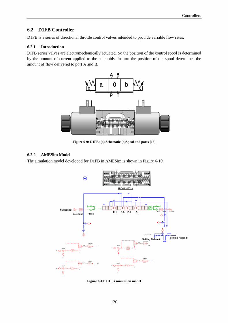
Controllers
120
6.2 D1FB Controller
D1FB is a series of directional throttle control valves intended to provide variable flow rates.
6.2.1 Introduction
DIFB series valves are electromechanically actuated. So the position of the control spool is determined
by the amount of current applied to the solenoids. In turn the position of the spool determines the
amount of flow delivered to port A and B.
Figure 6-9: D1FB: (a) Schematic (b)Spool and ports [15]
6.2.2 AMESim Model
The simulation model developed for D1FB in AMESim is shown in Figure 6-10.
Figure 6-10: D1FB simulation model

Controllers
121
6.2.3 Testing
Figure 6-12 shows the relation between the input current signal and the flow for a D1FB control with
E01H spool. As we can see, the simulated and theoretical characteristics correspond closely with each
other. The slight difference between the simulated and the theoretical curves can be contributed to a
simplification made regarding the shape of the metering holes on the spool bushing. In the simulation
model it is assumed that the metering holes are circular in shape. However in reality these holes have a
shape similar to a square. Therefore, as the spool moves in the bushing, the cross sectional flow area is
slightly different resulting in slight deviation between the theoretical and simulated curves.
Figure 6-11: Metering hole on the bushing (a) Actual (b) Simulation model
Figure 6-12: D1FB: Input signal and flow characteristics (a) Theoretical [10] (b) Simulated
The spool type E01H has a maximum flow limit for a given pressure drop shown in Figure 6-13. We
can see from the figure a good level of agreement exists between the simulated and theoretical results.
This flow limit is implemented in the simulation model using a variable orifice as shown in Figure
6-14. The area of this orifice is adjusted by using a look up table. This look up table takes in the

Controllers
122
current pressure difference across a metering edge and outputs the corresponding maximum flow that
can pass through it. By using the flow and pressure difference an appropriate area of the orifice is
calculated using the basic flow equation;
Figure 6-13: Flow limit (a) Theoretical [16] (b) Simulated
Figure 6-14: Flow limit implementation
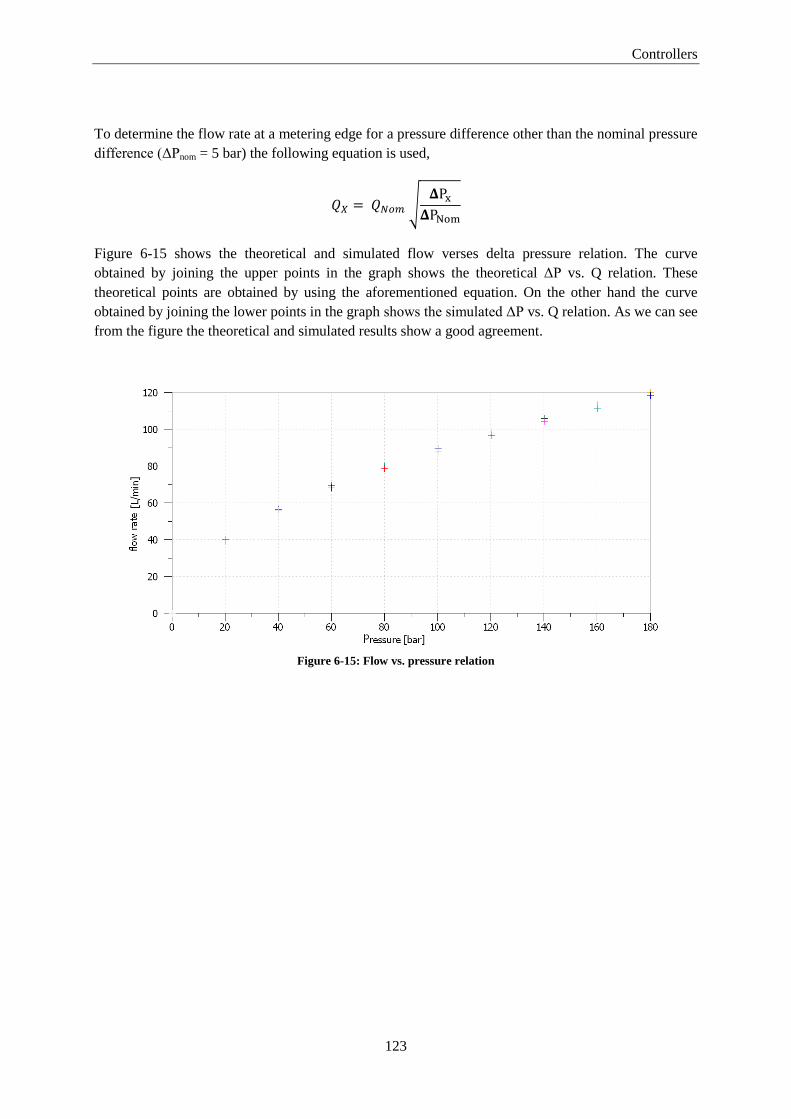
Controllers
123
To determine the flow rate at a metering edge for a pressure difference other than the nominal pressure
difference (ΔPnom = 5 bar) the following equation is used,
Figure 6-15 shows the theoretical and simulated flow verses delta pressure relation. The curve
obtained by joining the upper points in the graph shows the theoretical ΔP vs. Q relation. These
theoretical points are obtained by using the aforementioned equation. On the other hand the curve
obtained by joining the lower points in the graph shows the simulated ΔP vs. Q relation. As we can see
from the figure the theoretical and simulated results show a good agreement.
Figure 6-15: Flow vs. pressure relation

Controllers
124
6.3 HP Control
The HP control (hydraulic proportional control) is intended for applications where continuously
variable shaft speed is required. A prime example of such an application is a hydrostatic transmission.
6.3.1 Introduction
The HP proportional control provides continuously variable displacement for a hydraulic motor. A
hydraulic pilot pressure is used to control and adjust the displacement in a HP controller. The
schematic for this control is shown in Figure 6-16
.
Figure 6-16: HP Control: Schematic
Figure 6-16 shows the hardware level implementation of the HP control. A decrease in the pilot
pressure at port X5 causes the servo spool to move towards the right side. This movement of the servo
spool directs the flow into the right setting piston chamber. This in turn, displaces the setting piston
towards the left side. From the figure, we can see that a leftward movement of the setting piston would
result in an increase in the swivel angle. To summarize, a decrease in the pilot pressure would result in
an increase in the displacement setting and vice versa.
Figure 6-17: HP control function [17]

Controllers
125
In the HP control, normally the setting piston stays in the maximum displacement position until a pilot
pressure greater than the threshold pressure is applied as shown Figure 6-18. When a sufficiently large
pilot pressure is applied the setting piston displacement starts to decrease. The change in the
displacement is directly proportional to the applied modulating pressure. Both the threshold and
modulating pressures are adjustable.
Figure 6-18: Pressure vs. displacement [17]
6.3.2 AMESim Model
The simulation model developed in AMESim for the HP control is shown in Figure 6-19.
Figure 6-19: HP Control: AMESim model

Controllers
126
6.3.3 Testing
The displacement versus pressure curve obtained from the simulation model is shown is Figure 6-20.
In the simulation mode, like the actual controller, the threshold and the modulating pressures are
adjustable. By comparing Figure 6-18 and Figure 6-20 we can see that the behavior of the simulation
model is identical to the theoretical curve.
Figure 6-20: Displacement vs. pressure (simulated)

7 Validation
Development of the generic simulation model is succeeded by a validation phase. The purpose,
methodology and the results obtained during this phase are presented in this chapter.
7.1 Purpose
To use any simulation model in a practical scenario it is vital to quantify the level of accuracy offered
by the model. This is normally done by comparing the simulated results obtained from the simulation
model with experimental results obtained from the actual hardware. Through validation of the model
one can increase the level of confidence of the user on the simulation model. Moreover, by comparing
simulated and actual results identification and rectification of inaccuracies or errors in the model can
be done as well.
7.2 Approach
The methodology or the approach followed in the validation phase is quite straight forward. It can be
summari ed as “If the simulation model is fed with actual/experimental data then the output from the
simulation model should also match the actual/experimental data.” If this is not the case then the
simulation model fails to accurately represent a pump or a motor under consideration.
It is virtually impossible to develop a simulation model that fully corresponds to actual results in all
aspects. So, a tolerance or an acceptable amount of deviation of the simulation results from the actual
results is usually used.
7.3 Scope
The authentication process of a simulation model can be divided into two main steps;
a) Verification
b) Validation
a) Verification
Verification is the first step of this process and predominately deals with the correctness of the
model. In this step each part of the model is individually analyzed by observing whether the
direction and magnitude of the results are reasonable. Afterwards, effect of an individual
component on the behavior of the complete system is observed and analyzed for correctness in
a similar manner. However the level of difficulty in predicting the correct effect of a certain
component on the complete system increases rapidly with the size of the system. Therefore it
is usually difficult to correctly predict how a certain component in the model will affect the
behavior of the overall system especially in mid to large sized systems.
Moreover, this verification step is also useful in identifying some fundamental errors in the
model. As mentioned earlier, this generic simulation model needs to accurately represent three

Validation
128
inline and three bent-axis pumps and motor series. Therefore this verification step is carried
out for all of these six pumps and motors series.
b) Validation
Once it has been made sure that the simulation models are a correct overall representation of a
pump or a motor, one needs to check for the accuracy of this representation. This judgment
about the accuracy of the model is carried out in a step called the validation. The validation is
usually performed by comparing the results from the simulation model with the measurements
obtained from the actual system under same inputs and running conditions. However,
sometimes it is also possible to validate some parts of a simulation model by using results
from another simulation model which has been already validated and benchmarked.
As compared to the verification phase the validation phase is more thorough and consequently
requires more time. As a result validation of only two hydraulic units, one of inline type and
other of a bent axis type, is carried out. The two hydraulic units chosen for the validation
process are PVplus and C24, mainly because of the presence and availability of abundant
test/experimental data for these units. Both the units are representative of their corresponding
design types i.e. inline and bent axis. Thus the observations made during this validation phase
are applicable and transferrable to other pumps and motors as well.
7.4 Workflow
The procedure followed during the validation process is shown in Figure 7-1. The workflow followed
during the validation phase can be divided into two main activities; data acquisition and simulation.
a) Data Acquisition
In this step the data which is either required as an input to the simulation model or as an
output (data against which the simulation results will be compared) are measured, filtered and
put in an AMESim compatible format.
As mentioned before, large amount of test/experimental data is available spanning almost all
the working pressure, speed and displacement ranges. As this data covers almost all the
working points of a pump or a motor, it is used for validating the simulation model. The data
obtained from such tests is usually noisy. If noisy data is fed into a simulation model then the
time to complete a simulation (simulation time) becomes too large. The reason for a large
simulation time in this case is that the solver tries to lower the time step in presence of a noise
in the signal. The noise usually has a frequency many times higher than the actual signal.
Moreover, a noisy input not only increases the simulation time, it could also result in
simulation terminating prematurely. This premature termination of a simulation usually occurs
when the solver reaches its lower time step limit. Therefore it is necessary to filter the
experimental data using a low pass filter. Furthermore, to reduce the simulation time, it is also
sometime necessary to resample the experimental data to a lower sampling rate, thus reducing
the number of data points the solver needs to solve. In some cases it is also necessary to
smooth out the data to avoid catastrophic errors during the simulation. All these data
operations are very effective in reducing the simulation time and avoiding any errors during
the simulation, however extreme care should be taken to preserve the shape and magnitude of
the original signal. So, there is always a compromise between the reduction of simulation time
and keeping the shape of the original signal intact.

Validation
129
The signal processing phase results in a data suitable for a simulation however it is not in an
AMESim compatible format. A data file contains multiple channels where every channel
contains data for a single variable (e.g. shaft speed, high pressure etc). Every data file needs to
be broken into individual text files. In these text files the data needs to be in a specific format
so that it is compatible with AMESim. For more details on AMESim compatible data formats
refer to AMESim Help [12]. At this stage this processed data is ready to be put in an
AMESim simulation model.
b) Simulation
In the simulation part of the validation, the processed experimental data is fed into the
simulation model. Afterwards, an iterative process of performing a simulation and comparing
the simulation results with the experimental data is carried out. The fine tuning of the
simulation model is performed until the error between the simulation results and the
experimental data is negligible. The parameters used to fine tune the model are the coefficient
of frictions and scaling factors. These scaling factors are introduced to compensate for
inaccuracies in modeling a certain force from a component. These inaccuracies usually arise
from assumptions made while modeling. So by using such a scaling factor a force calculated
by a certain component can be modified up to +/- 3 % of its original value.
Figure 7-1: Validation process

Validation
130
7.5 PVplus 360: Validation
The simulation model, experimental data and results obtained during the validation process of the
PVplus 360 inline axial piston pump are presented in the following section.
7.5.1 System Diagram
The simulation model used for the validation process is shown in Figure 7-2.
Figure 7-2: PVplus simulation model
7.5.2 Experimental Data
The following four experimental parameters were used for the validation of this pump.
Shaft speed
Compensator pressure
High pressure
LVDT signal
7.5.2.1 Inputs
Shaft speed, compensator pressure and high pressure are fed into the simulation model (referred here
as inputs). Shaft speed is the rotational velocity of the pump shaft. It is measured at the point where
the prime mover (in this case an electric motor) is coupled to the pump. Compensator pressure is the
pressure in the setting piston chamber due to the flow from the controller. The high pressure, as the
name implies, is the pressure measured at the high pressure or the output port of the pump.
7.5.2.2 Output/Target
The experimental parameter against which the simulation results are tested is the LVDT signal. LVDT
(Linear Variable Differential Transformer) is a type of electrical transformer used to measure
linear\translational displacement [13]. The LVDT indirectly measures the swivel angle by measuring
the linear displacement of the setting piston.
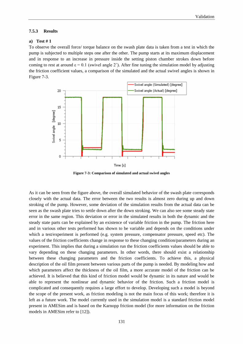
Validation
131
7.5.3 Results
a) Test # 1
To observe the overall force/ torque balance on the swash plate data is taken from a test in which the
pump is subjected to multiple steps one after the other. The pump starts at its maximum displacement
and in response to an increase in pressure inside the setting piston chamber strokes down before
coming to rest at around ε .1 (swivel angle 2˚). After fine tuning the simulation model by adjusting
the friction coefficient values, a comparison of the simulated and the actual swivel angles is shown in
Figure 7-3.
Figure 7-3: Comparison of simulated and actual swivel angles
As it can be seen from the figure above, the overall simulated behavior of the swash plate corresponds
closely with the actual data. The error between the two results is almost zero during up and down
stroking of the pump. However, some deviation of the simulation results from the actual data can be
seen as the swash plate tries to settle down after the down stroking. We can also see some steady state
error in the same region. This deviation or error in the simulated results in both the dynamic and the
steady state parts can be explained by an existence of variable friction in the pump. The friction here
and in various other tests performed has shown to be variable and depends on the conditions under
which a test/experiment is performed (e.g. system pressure, compensator pressure, speed etc). The
values of the friction coefficients change in response to these changing condition/parameters during an
experiment. This implies that during a simulation run the friction coefficients values should be able to
vary depending on these changing parameters. In other words, there should exist a relationship
between these changing parameters and the friction coefficients. To achieve this, a physical
description of the oil film present between various parts of the pump is needed. By modeling how and
which parameters affect the thickness of the oil film, a more accurate model of the friction can be
achieved. It is believed that this kind of friction model would be dynamic in its nature and would be
able to represent the nonlinear and dynamic behavior of the friction. Such a friction model is
complicated and consequently requires a large effort to develop. Developing such a model is beyond
the scope of the present work, as friction modeling is not the main focus of this work; therefore it is
left as a future work. The model currently used in the simulation model is a standard friction model
present in AMESim and is based on the Karnopp friction model (for more information on the friction
models in AMESim refer to [12]).
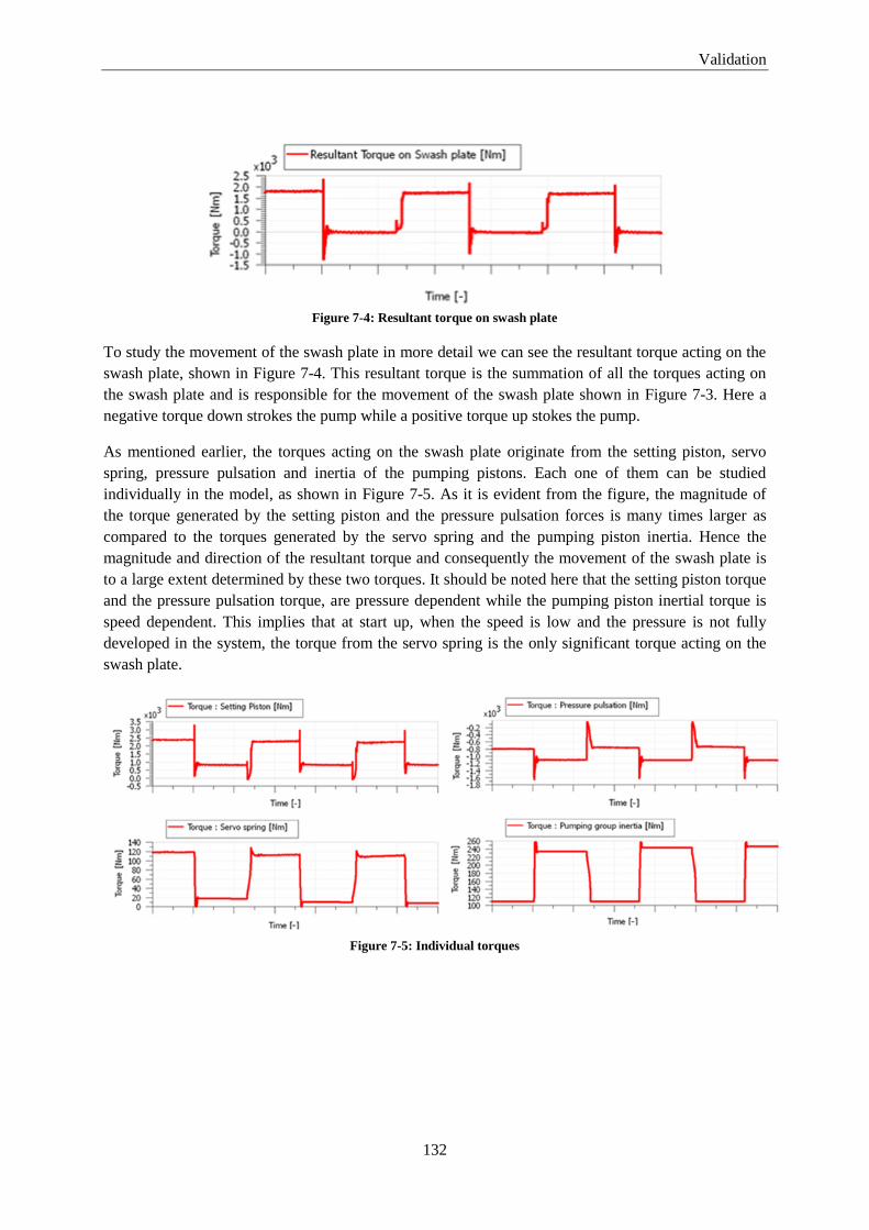
Validation
132
Figure 7-4: Resultant torque on swash plate
To study the movement of the swash plate in more detail we can see the resultant torque acting on the
swash plate, shown in Figure 7-4. This resultant torque is the summation of all the torques acting on
the swash plate and is responsible for the movement of the swash plate shown in Figure 7-3. Here a
negative torque down strokes the pump while a positive torque up stokes the pump.
As mentioned earlier, the torques acting on the swash plate originate from the setting piston, servo
spring, pressure pulsation and inertia of the pumping pistons. Each one of them can be studied
individually in the model, as shown in Figure 7-5. As it is evident from the figure, the magnitude of
the torque generated by the setting piston and the pressure pulsation forces is many times larger as
compared to the torques generated by the servo spring and the pumping piston inertia. Hence the
magnitude and direction of the resultant torque and consequently the movement of the swash plate is
to a large extent determined by these two torques. It should be noted here that the setting piston torque
and the pressure pulsation torque, are pressure dependent while the pumping piston inertial torque is
speed dependent. This implies that at start up, when the speed is low and the pressure is not fully
developed in the system, the torque from the servo spring is the only significant torque acting on the
swash plate.
Figure 7-5: Individual torques

Validation
133
b) Test# 2
To validate the dynamic response of the swash plate, data is taken from a test where a step is applied
to the swash plate. The test from which the data is obtained is very similar to the test in the previous
section; however, the two tests were performed at two different pressure levels. As in the previous
case, the pump starts at its maximum displacement and strokes down in response to a step applied by
the compensator. The simulated and the actual dynamic behavior of the swash plate are shown Figure
7-6. As we can see from the figure, the error (represented by the blue curve) between the simulated
and the actual swivel angles is small. Moreover, the steady state error is almost zero. This deviation
between the simulated and the actual results can also be explained by the presence of variable (or
parameter dependent) friction. In the figure, we can observe that the simulated swash plate after the
first peak moves and remains stationary for a brief period before moving again. This behavior points
towards a ‘stick-slip’ phenomenon, which is also related to friction. When the simulated swash plate
reaches the peak and changes direction the velocity of the swash plate goes to zero brining stiction into
effect. The value of the stiction is large enough to stop the swash plate from moving. Therefore the
simulated swash plate remains stationary until enough torque is applied on it. A simple and straight
forward solution to rectify this deviation from the actual response is to decrease the stiction coefficient
value; however doing so would result in a larger error in the earlier part of the response. Therefore a
friction model which is able to change its friction coefficient values based on some system parameters
is needed. Although a dynamic friction model would increase the accuracy of the simulation model,
even with a static friction model like the one used here, sufficiently accurate results could be obtained.
Figure 7-6: Comparison of simulated and actual swivel angles
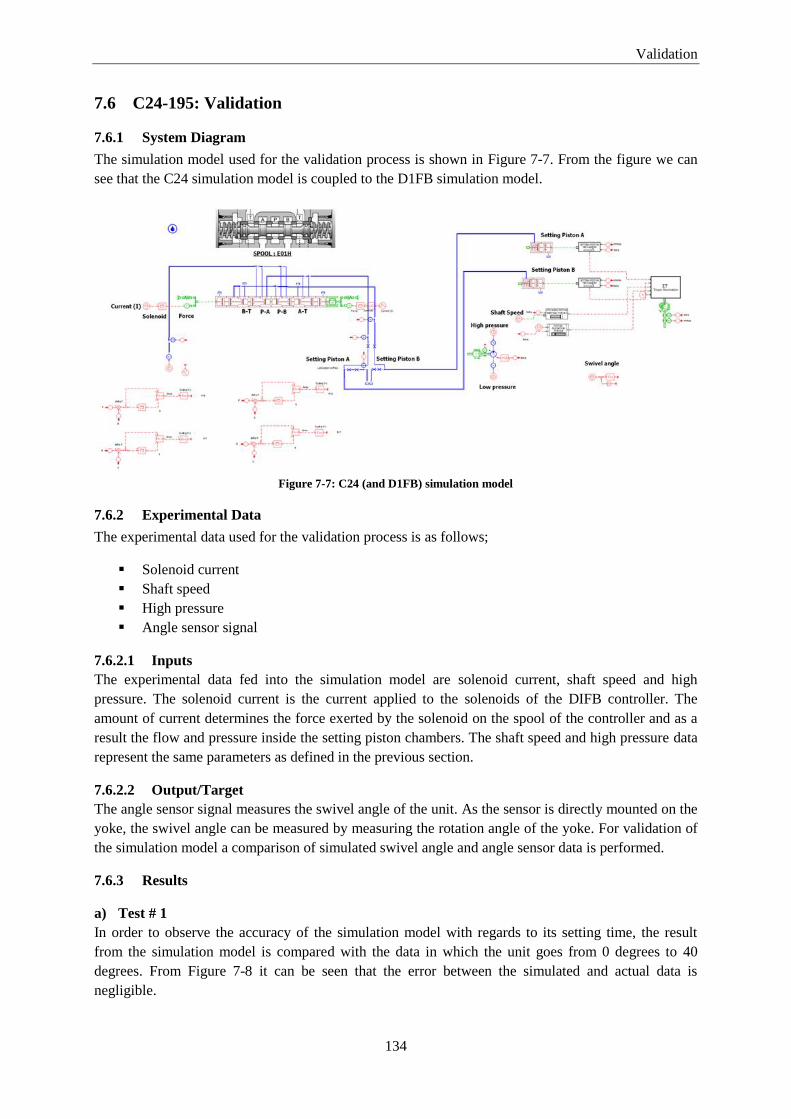
Validation
134
7.6 C24-195: Validation
7.6.1 System Diagram
The simulation model used for the validation process is shown in Figure 7-7. From the figure we can
see that the C24 simulation model is coupled to the D1FB simulation model.
Figure 7-7: C24 (and D1FB) simulation model
7.6.2 Experimental Data
The experimental data used for the validation process is as follows;
Solenoid current
Shaft speed
High pressure
Angle sensor signal
7.6.2.1 Inputs
The experimental data fed into the simulation model are solenoid current, shaft speed and high
pressure. The solenoid current is the current applied to the solenoids of the DIFB controller. The
amount of current determines the force exerted by the solenoid on the spool of the controller and as a
result the flow and pressure inside the setting piston chambers. The shaft speed and high pressure data
represent the same parameters as defined in the previous section.
7.6.2.2 Output/Target
The angle sensor signal measures the swivel angle of the unit. As the sensor is directly mounted on the
yoke, the swivel angle can be measured by measuring the rotation angle of the yoke. For validation of
the simulation model a comparison of simulated swivel angle and angle sensor data is performed.
7.6.3 Results
a) Test # 1
In order to observe the accuracy of the simulation model with regards to its setting time, the result
from the simulation model is compared with the data in which the unit goes from 0 degrees to 40
degrees. From Figure 7-8 it can be seen that the error between the simulated and actual data is
negligible.
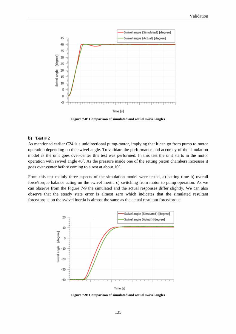
Validation
135
Figure 7-8: Comparison of simulated and actual swivel angles
b) Test # 2
As mentioned earlier C24 is a unidirectional pump-motor, implying that it can go from pump to motor
operation depending on the swivel angle. To validate the performance and accuracy of the simulation
model as the unit goes over-center this test was performed. In this test the unit starts in the motor
operation with swivel angle 40˚. As the pressure inside one of the setting piston chambers increases it
goes over center before coming to a rest at about 10˚.
From this test mainly three aspects of the simulation model were tested, a) setting time b) overall
force\torque balance acting on the swivel inertia c) switching from motor to pump operation. As we
can observe from the Figure 7-9 the simulated and the actual responses differ slightly. We can also
observe that the steady state error is almost zero which indicates that the simulated resultant
force/torque on the swivel inertia is almost the same as the actual resultant force/torque.
Figure 7-9: Comparison of simulated and actual swivel angles

Validation
136
It was observed during the validation process that the magnitude of the friction in bent axis units is
significantly smaller as compared to an inline unit. In other words, in a bent axis unit the influence of
the friction on the overall behavior of the unit is less as compared to an in-line machine. This smaller
range in which the friction can vary for a bent axis unit also reduces the time and effort required to
fine tune a simulation model as compared to an inline machine.
7.7 Auto-Tuning: Optimization
In the fine tuning phase of the validation process, the friction values are adjusted so as to minimize the
error between the simulated and actual results. The fine tuning for the validation results presented
above is done manually. This fine tuning phase is a repetitive, time and effort expensive task.
Therefore, to minimize the effort required by the user to fine tune a model, an optimization routine is
developed. This optimization routine tries to minimize the error between the simulated and the actual
results by adjusting the friction values within predefined limits. This optimization falls under the
category of simulation based optimization. So every objective function evaluation is actually a
result/output of a simulation run.
7.7.1 Mathematical Formulation
The aforementioned optimization routine can be written mathematically as;
Objective function;
Where
Swivel angle:
Penalty function weight:
Penalty function:
Subject to constraints;
Coefficient of viscous friction
Coulomb friction torque
Stiction friction torque

Validation
137
7.7.2 Algorithm
The following two optimization algorithms were used.
a) NLQPL (Non-linear Programming by Quadratic Lagrangian)
b) Genetic algorithm
The time required by NLQPL to converge to a solution is significantly less than the time needed by the
genetic algorithm. However NLPQL being a gradient based method resulted in many runs converging
to local optima. On the other hand genetic algorithm is many times more robust when it comes to
finding the global or true optimum of a problem. Therefore NLPQL was abandoned in favour of
genetic algorithm. The design exploration tool in AMESim was used for the implementation of the
optimization routine (for more details on design exploration tool refer to [12]).
7.7.3 Results
As mentioned above genetic algorithm was used for the optimization routine. The parameters for the
algorithm are summarized in Table 7-1.
Parameter Value Number of Individuals/ generation 50
Reproduction ratio 75
Max number of generation 22
Mutation probability 25
Mutation amplitude 0.3
Seed(s) 3
Table 7-1: Genetic algorithm parameters
Figure 7-10(a) shows the objective function value for each iteration. This objective function value
indicates the amount of error between the simulated and actual results. From the figure we can see that
the error is large in the start of the optimization process however the algorithm tires to reduce it until
the optimization converges or some other termination criteria is met. Figure 7-10(b) shows the
progress of the optimization variables (friction coefficients) during the optimization routine. The
values of optimization variables change rapidly in the start of the optimization. This variation in the
values of the optimization variables decreases as the optimization progresses. As we can see in the
figure these values do not change after some number of iterations indicating that the optimization has
converged to a solution. The result of this optimization process is called the ‘best individual’. This best
individual is basically a set of friction coefficient values resulting in minimum error between the
simulated and actual results. Figure 7-10(c) shows the comparison of the simulated and the actual
results with the optimal friction values applied to the simulation model.
It should be noted here that using an optimization routine as compared to manually fine tuning a
model significantly decreases the manual effort required by the user. Here the user is only required to
set up the optimization. On the other hand, the time required to reach a fine-tuned simulation model
does not always decrease when using an optimization routine. Instead it can increase especially when
using genetic algorithm. For results presented here a large number of individuals per generation and
maximum number of generation were used. This meant the optimization routine required a large
number of iterations (>800 iterations) and time (3-4 hours) to converge. However increasing these
algorithm parameters yielded a result closer to the global optimum (i.e. Error = 0).

Validation
138
Figure 7-10: Optimization results (a) Objective function value (b) Optimization variables (c) Simulated and actual
response

Validation
139
Figure 7-11: Optimization results (a) Objective function value (b) Optimization variables (c) Simulated and actual
response


8 Documentation
For all created component and their submodel a corresponding help section is developed in AMESim.
Through this help section a user can easily understand the input/output variables, usage, required
parameters and the mathematical equations used to create a submodel. This help section is similar to
the AMESim standard help section, in its structure. It contains the icon, a brief description and usage
of the submodel. The inputs that are required by the submodel and the outputs that are generated along
with their respective port numbers are also presented. This is followed by a list of input and output
variables along with corresponding variable names and units. All the parameters required as inputs
from the user are also listed under the real parameters. Finally, all the mathematical equations and the
corresponding diagrams used to create a submodel are also provided in this help section. An example
of such a help section is shown is Figure 8-1.
Figure 8-1: Help section - Example


9 Conclusions
From the work presented above the following major conclusions can be drawn.
1. Generic Model
The prime motivation of carrying out this thesis work was to find out if it is possible to accurately
represent both inline and bent axis piston machines with a single generic model. As a result of the
thesis work, one can safely say that it is feasible to create a generic simulation model representing
both inline and bent axis machines. Not only is such a generic model feasible it also offers a lot of
advantages when comparing to the conventional way of creating simulation models. Some of these
advantages include a single model structure to represent a large number of machines, easier
comparison of different machines, less file management and possible reduction in development
cost. So such a generic approach for simulation model development offers a very viable alternative
to the conventional way of modeling especially when dealing with a large number of machines.
2. Friction Models
Friction is a complex phenomenon to model due to its non linearity. Moreover, friction is dynamic
in its nature especially when a body goes from a stationary to a moving/rotational state. The
friction model used in the generic simulation model is a static friction model. Such a static model
does not accurately represent the dynamic behavior of the friction. In addition to that, it was also
observed that the amount of friction present in a hydraulic machine is dependent on the working
conditions (e.g. system pressure, barrel rotation speed, oil temperature etc). So as these working
conditions change, friction in a hydraulic machine changes as well. So a much more advanced
friction model is needed to accurately represent the friction in a machine. In spite of these
relatively simple friction models, sufficiently good agreement between the simulated and
experimental data was achieved. This means that although an advance friction model would
increase the accuracy of the simulation model by better describing the friction phenomenon,
simple friction models can also be used.
3. Minimum Error Propagation
The generic model developed during this thesis work is modular in its structure. Using a modular
approach to build a simulation model offers a great advantage by isolating the error locally within
a module. In other words, this modular approach minimizes the error propagation through the
model. So in case of a faulty module in a simulation model, the fault or the error remains localized
and does not propagate and effect other parts of the model. In a modular simulation model a faulty
module can be easily replaced by a working module or even bypassed, if that module is not
critical. On the other hand, a model where every part is dependent on each other, a faulty part
would make the complete model faulty and useless. In a modular approach error detection is also
relatively simpler to perform.

Conclusions
144
4. User Interface
The user-interface presented in the thesis work connecting the user with generic model, provides a
good platform for transferring high-level parameters from the user into low level parameters
required by the generic model. Example of a high level information is the maximum swivel angle
of a pump or a motor, while the corresponding low level parameter is ‘rotation inertia end stop
angle 1’. So a high level parameter is some knowledge or parameter easily understandable for a
user, while a low level parameter lies on the other end of the spectrum. Normally, a low level
parameter is not very intuitive and requires a good knowledge about the simulation model to
understand. This user interface only requires information that is easier for the user to understand
and automatically applies those parameters into corresponding simulation model parameters.
Through this automatic assignment of simulation model parameters the need for detail knowledge
regarding the simulation model to perform simulations is eliminated.
5. Flexibility
As described above, a modular approach has been used for the development of the generic
simulation model. This modular structure is flexible for incorporating new changes in the model.
For example to create simulation models of existing pumps and motors not modeled during the
thesis work. One only needs to develop a small number of additional modules. These additional
modules would be identical in structure to the existing modules with some changes in
mathematical equations describing the relation of input with the outputs. The main advantage of
this approach is that one does not need to rethink the whole structure of the simulation model
when modeling other pumps and motors.
10 Future Work
The thesis work explores a novel way to model hydraulic machines. The work performed during this
thesis could serve as a platform for further refining and developing this new methodology for model
development. As future work to this master thesis the following recommendations are presented;
1. Generic model for controllers
The generic approach, methodology and structure developed for modeling hydraulic pumps
and motors could be applied to model other components and machines. As a start it is
recommended that a generic model, based on the same approach presented in this work, could
be developed for controllers as well. Due to somewhat inherent modular structure of the
controllers it might be relatively easier to develop such a generic modular simulation model as
compared to hydraulic pumps and motors.
2. Populate Parameter Library
Currently, the parameter library in the user-interface contains parameters of only a limited
number of the pump and motor sizes. This in turn limits the number of pumps and motor the
generic model can represent. It is recommended that the parameter library be populated to
include the parameters of all pump and motor series sizes.
3. Extended Validation
As described in chapter 7 validation of only two hydraulic units (PVplus and C24) is carried
out. To increase the level of confidence in the simulation model it is recommended that this
validation process could be extended to validate models for other pumps and motors (i.e. P2,
VP1, V12 and V14). During the validation of these machines same methodology presented in
this work could be used.
4. Detail Friction Models
As described earlier, a static friction model has been used to represent the friction present in a
pump or a motor. It is recommended that a detailed friction model is developed, that will
improve the accuracy of the simulation results. Such a model should describe the development
of oil film between various moving components in a pump or a motor and factors affecting its
thickness. This model could be developed either within the current simulation model as an
extension or as a standalone model which could be coupled to the generic simulation model.

11 References
[1] Ivantysyn, J., & Ivantysynova, M., Hydrostatic pumps and motors. (First English Edition).
Wurzburg, Germany: Vogel Verlag und Druck GmbH, 2001, pp100.
[2] Jeffery W. Dobchuk, “Sub-component level modeling of a Variable displacement axial piston
Pump”, Department of Mechanical Engineering, University of Saskatchewan, Canada, 2 .
[3] Parr A., Hydraulics and Pneumatics: A Technician's and Engineer's Guide 3rd Edition,
Butterworth-Heinemann, 2011, pp31-47.
[4] Hussian Z., Abdullah Z., Alimuddin Z., Basic Fluid Mechanics and Hydraulic Machines, BS
Publications, 2008, Chap 2.
[5] Noah D. and ikreadam A., “The control tor ue on the swash plate of an Axial Piston Pump
utili ing Piston Bore Springs”, Journal of Dynamic Systems, Measurements and Control, Vol.
123, September, 2011, pp. 471-478.
[6] N.D. Manring and R.E. Johnson, “Modeling and Designing a Variable displacement Open
Loop Pump”, Journal of Dynamic Systems, Measurements and Control, Vol. 11 , June, 1996,
pp. 267-271.
[7] Alessandro R., Salvatore M. and Nicola N., “Modeling a Variable Displacement Axial Piston
Pump in a Multibody Simulation Environment”, Transactions of ASME, Vol. 12 , July 2 ,
pp. 456-468.
[8] Daniel Anderson, “Modeling and Simulation of Volumetric Hydraulic Pumps in AMESim”,
Department of Management and Engineering (IEI), LMS Imagine, Lyon Office.
[9] Wikipedia, http://en.wikipedia.org/wiki/Hydraulic_motor, , Last accessed 18 Aug 2011
[10] Wikipedia, http://www.tpub.com/content/engine/14105/css/14105_47.htm, Last accessed 18
Aug 2011
[11] Wikipedia, http://en.wikipedia.org/wiki/Hydraulic_pump, Last accessed 18 Aug 2011
[12] AMESim v11, AMESim help

References
148
[13] Wikipedia, Linear Variable differential transformer http://en.wikipedia.org/wiki/Linear
_variable_differential_transformer, Last accessed 7 Sept 2011.
[14] Parker Hannifin catalogue HY30-3245/UK
[15] Parker Hannifin catalogue HY14-2550/US
[16] Parker Hannifin catalogue HY30-8223/UK
[17] LMS website, http://www.lmsintl.com, Last accessed 2 Sept 2011

12 Appendix-A
Model Application Example
Some examples of the possible scenarios where the generic simulation model can be used are
presented in this section.
12.1 Internal Pump study
12.1.1 Pv plus: Chain Length vs. Setting Piston Torque/Force
As an example of an internal pump study, the generic simulation model can be used to study the
relation between the length of the chain joining the setting piston to the swivel inertia and the torque
generated by the setting piston on the swivel inertia. This relation is shown in Figure 12-1.
Figure 12-1: Chain length vs. setting piston torque
12.1.2 Pumping Piston Mass vs. Pumping Group Inertial Torque
Another example of an internal pump study would be to study the effect of the mass of a pumping
piston on the resultant inertial torque generated by the pumping group acting on the swivel inertia.
Figure 12-2 shows a linear relation between the two parameters.

Appendix-A
150
Figure 12-2: Pumping piston mass vs. pumping group inertial torque
12.1.3 Setting Time vs. Lubrication Orifice Diameter
Studying the impact of changing the lubrication orifice diameter on the setting time of the machine is
another example of an internal pump study. The results are presented in the Figure 12-3.
Figure 12-3: (a) Setting time (b) Setting time vs. lubrication orifice diameter

Appendix-A
151
12.2 System Investigation
An example of a system investigation is presented in Figure 12-4. The system comprises of a PV plus
360 pump delivering fluid to a C24-195 pump-motor, which in this case is working as a motor. A
MMC controller is used to control the pump displacement while a D1FB control valve adjusts the C24
displacement. In AMESim supercomponents are used to implement the schematic as shown in Figure
12-5.
Figure 12-4: System level investigation
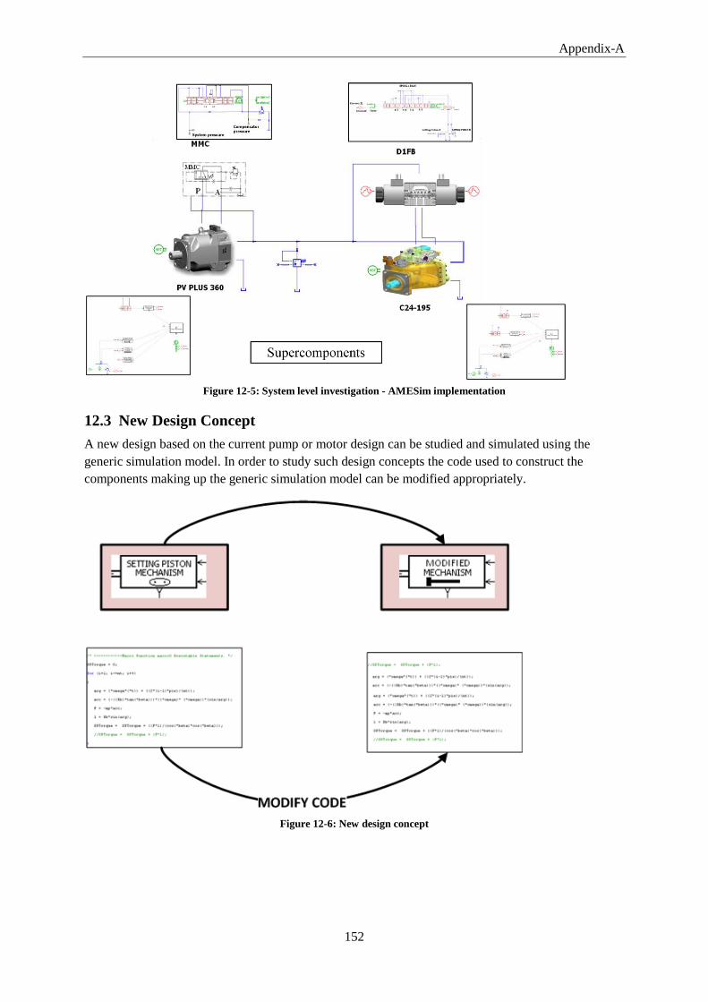
Appendix-A
152
Figure 12-5: System level investigation - AMESim implementation
12.3 New Design Concept
A new design based on the current pump or motor design can be studied and simulated using the
generic simulation model. In order to study such design concepts the code used to construct the
components making up the generic simulation model can be modified appropriately.
Figure 12-6: New design concept

13 Appendix-B
Pump motor supercomponent
A unidirectional pump-motor supercomponent is created. Figure 13-1 shows the ports and the
input/output variables associated with them, while Figure 13-2 shows the implementation of the
supercomponent in AMESim.
Figure 13-1: Pump-motor supercomponent external variables
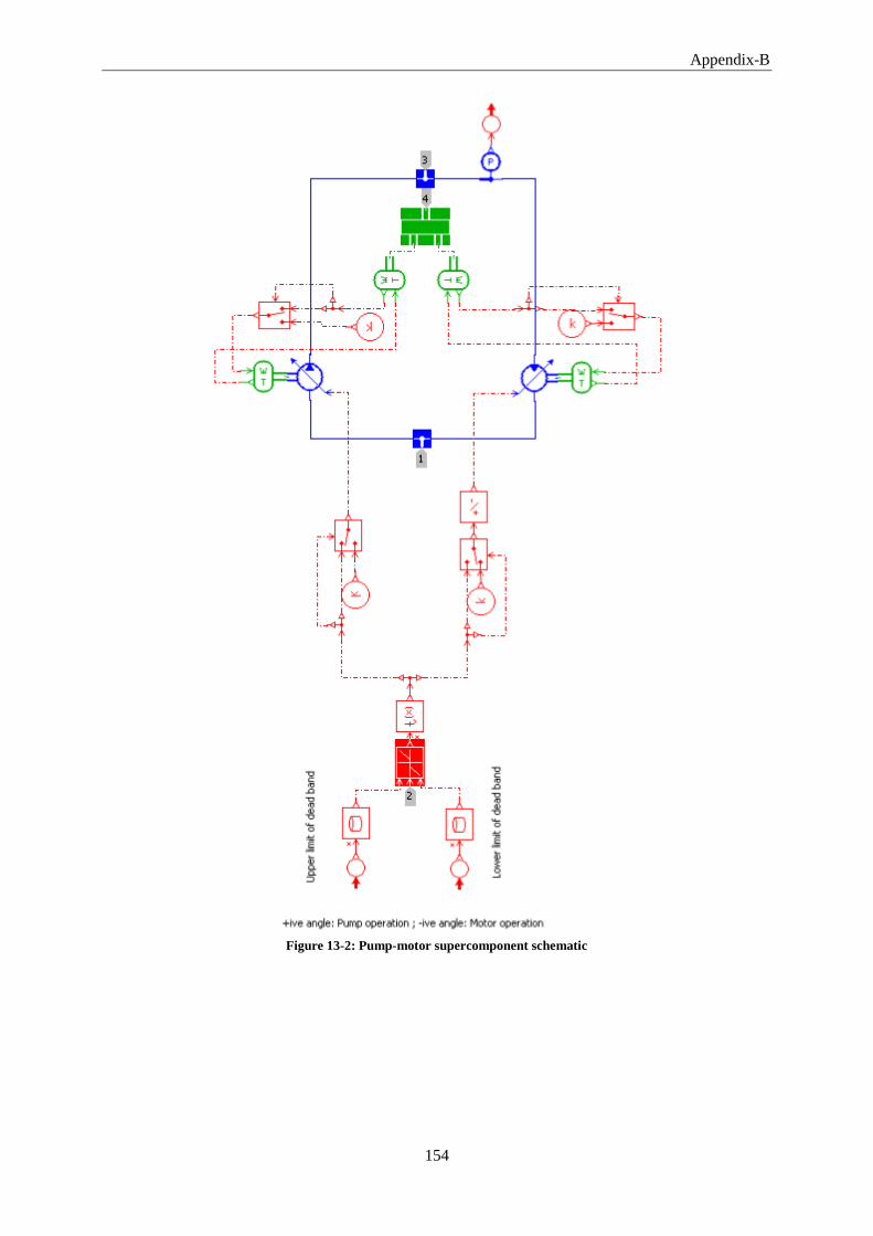
Appendix-B
154
Figure 13-2: Pump-motor supercomponent schematic

Appendix-B
155
13.1 Motor
To test the functionality of the created supercomponent, it is run only as a motor and its results are
compared with a standard motor in AMESim. Afterwards the supercomponent is run as a pump, and
the results are compared with a standard pump in AMESim.
Figure 13-3: (a) Standard AMESim motor (b) Supercomponent running as a motor
Figure 13-4: Standard AMESim motor and pump-motor supercomponent (a) flow (b) pressure (c) shaft speed
comparison

Appendix-B
156
13.2 Pump
Figure 13-5: (a) Standard AMESim pump (b) Supercomponent running as a pump
Figure 13-6: Standard AMESim pump and pump-motor supercomponent (a) flow (b) pressure (c) shaft speed
comparison

Appendix-B
157
13.3 Pump-Motor
To test the supercomponent working as a pump-motor, it is placed in a hydraulic system to regenerate
energy shown in Figure 13-7. Initially the pump-motor works as a motor speeding up the flywheel
attached to its shaft. After some time by changing the swivel angle, the pump-motor is operated like a
pump. Now the kinetic energy stored in the rotating flywheel is used by this pump to deliver additional
flow to the load. The hydraulic load in the system is modeled using a simple orifice. Results from this
test are presented in Figure 13-8.
Figure 13-7: Pump-motor used to regenerate energy using a flywheel
Figure 13-8: Pump-motor (a) swivel angle (b) shaft speed (c) flow (d) total flow


14 Appendix-C
Created Components, Submodels
& Supercomponents List
Component Submodel Pump/ Motor
series Description
Setting piston
mechanism
Chain PV Plus
Models how the setting
piston is connected to
swivel inertia.
Ball VP1 VP1
Ball VP1 Lower VP1
Chain mechanism P2 P2
Pin mechanism V12 v14 V12 & V14
Setting piston mechanismA C24 C24
Setting piston mechanismB C24 C24
Servo spring Pin mechanism Pv Plus Models how the Servo
spring is connected to
swivel inertia.
Servo spring P2 P2
Servo spring VP1 VP1
Stroking piston
inertial forces Direct connection PV Plus & P2 Calculates the torque on
the swivel inertia due to
inertia of the pumping
group.
Spring connection VP1
C24 pumping piston C24, V12 & V14
Torque
Summation Torque Summation All
Sums up all the torques
and applies it to the
inertia.
Spring
Spring_01 Simple Spring
User can specify the
distance covered before
it engages (starts to
compress).
Piston
pulsation
torque
Piston pulsation torque All
Used to input the
pressure pulsation force
and position.
Table 14-1: Created components and submodels

Appendix-C
160
Super Component Submodel Pump/ Motor
series Description
Generic pump
motor PV Plus 360 PV Plus
Generic supercomponent to
model various pump and
motors.
(Mainly used for system-level
investigation.)
P2 075 VP1
VP1 095 VP1
C24 195 P2
V14 110 V12 & V14
V12 60 C24
MMC MMC MMC
Model for standard constant
pressure controller for PVplus.
D1FB D1FB D1FB
Model for D1FB controller
(C24). Spring connection VP1
C24 pumping piston C24, V12 & V14
Table 14-2: Created supercomponents


