GEOCHEMICAL CHARACTERIZATION OF MUDFLAT
AND MANGROVE SEDIMENTS IN ZUARI ESTUARY
Ph.D THESIS
By
Cheryl A. Noronha e D’Mello
M.Sc.
JULY, 2016

GEOCHEMICAL CHARACTERIZATION OF MUDFLAT AND MANGROVE
SEDIMENTS IN ZUARI ESTUARY
THESIS
SUBMITTED TO THE GOA UNIVERSITY FOR THE AWARD OF THE DEGREE OF
DOCTOR OF PHILOSOPHY
IN
MARINE SCIENCES
BY
CHERYL A. NORONHA E D’MELLO
M.Sc.
RESEARCH GUIDE
PROF. G. N. NAYAK
Department of Marine Sciences,
Goa University,
Taleigao, Goa, India -403206
JULY 2016

DEDICATED TO MY
FAMILY
STATEMENT
As required under the University ordinance OB.9.9 (iv), I state that the present thesis entitled
“GEOCHEMICAL CHARACTERIZATION OF MUDFLAT AND MANGROVE
SEDIMENTS IN ZUARI ESTUARY” is my original contribution and the same has not been
submitted on any other previous occasion. To the best of my knowledge, the present study is the
first comprehensive work of its kind from the area mentioned.
The literature related to the problem investigated has been cited. Due acknowledgements have
been made wherever facilities and suggestions have been availed of.
Place: Goa University
Date : 19th
April 2017
Mrs. Cheryl A. Noronha e D’Mello

CERTIFICATE
This is to certify that the thesis entitled, “GEOCHEMICAL CHARACTERIZATION OF
MUDFLAT AND MANGROVE SEDIMENTS IN ZUARI ESTUARY”, submitted by Mrs.
Cheryl A. Noronha e D’Mello for the award of the Degree of Doctor of Philosophy in Marine
Science is based on her original studies carried out by her under my supervision. The thesis or
any part thereof has not been previously submitted for any other degree, diploma, associateship,
fellowship or similar titles in any universities or institutions. This thesis represents independent
work carried out by the student.
Place: Goa University
Date: 19th
April 2017
Prof. G. N. Nayak
(Research Guide)
Department of Marine Sciences,
Goa University, Goa
Acknowledgements
First and foremost, I would like to express my sincere gratitude to my research guide and
supervisor Prof. G. N. Nayak, whose expertise, understanding, and patience, added considerably
to my research experience. His systematic guidance helped me in all the times of research and in
writing of this thesis. I would like to thank him for encouraging my work with many insightful
discussions and suggestions, and the great effort he put into training me in the scientific field.
I would also like to thank the FRC members, Dr. N. B. Bhosle, retired Scientist, NIO, Goa; Prof.
M. K. Janarthanam, Dean of the faculty of life sciences and environment; Prof. C. U. Rivonkar,
Head of the Department of Marine Sciences and Prof. G. N. Nayak, for their encouragement,
insightful comments, and thought provoking questions.
I wish to acknowledge Dr. S. R. Shetye, Vice Chancellor of Goa University and Prof. Y. V.
Reddy, Registrar and their subordinates for their support and administrative help throughout the
Ph.D. program. I also wish to thank Prof. Dileep Deobagkar, former Vice Chancellor of Goa
University and Prof. V. P. Kamat, former Registrar, for their support and encouragement.
I am grateful to Dr. S.W.A. Naqvi, Director, NIO, Goa for permitting me to carry out some of
the analysis at the institute. My sincere thanks go to Dr. V. P. Rao, Scientist, NIO, Goa, for
assistance in the clay mineralogy analysis and Dr. Pratima Kessarkar, Scientist, NIO, Goa, for
providing assistance in magnetic susceptibility measurements. Further, I wish to thank Dr. S.
Kurian, Dr. Lidita Khandeparkar, Dr. Lina Fernandes Scientists, NIO, Goa and technical officers
Mr. Girish Prabhu and Mr. B. G. Naik for their co-operation, support and suggestions during the
analysis. I also wish to thank Dr. Sangeeta Jadhav, Dr. R. Shynu and A. Prajith, NIO, Goa for
their help and support during the analysis.
My sincere thanks go to the faculty of department of Marine Sciences, Goa University, Prof. C.
U. Rivonkar, Prof. H. B. Menon, Dr. S. Upadhyay, Prof. V.M. Matta and Dr. A. Can, for their
encouragement.

I wish to acknowledge the non-teaching staff of the department of Marine Sciences, Mr.
Yeshwant Naik, Mr. Samrat Gaonkar, Mr. Shatrugan Shetgaonakar, Mr. Ratnakar Naik, Ms.
Reena Tari, Mrs. Mangal and Mrs. Concessao as well as the former staff, Mr. Ashok Parab and
Mr. Rosario for their help and support. I also wish to thank Prof. Savita Kerkar, Head of the
Department of Biotechnology, Prof. U.D. Muraleedharan, former Head of the Department of
Biotechnology, Prof. B. F. Rodrigues, Head of the Department of Botany and non-teaching staff
Mr. Redualdo Serrao, Mr. Ulhas and Mr. Martin from the Department of Biotechnology for their
kind help.
I am also grateful to my colleagues in research, Dr. Deepti Dessai, Dr. Lina Fernandes, Dr,
Ratnaprabha Siraswar, Dr. Samida Volvoikar, Dr. Anant Pande, Mr. Maheshwar Nasnodkar, Ms.
Maria Fernandes, Ms. Purnima Bejugam, Ms. Shabnam Choudhary, Mrs. Janhavi Kamat, Ms.
Tanu Hoskatta, Dr. Vinay Padte, Dr. Mahableshwar Hegde, Mr. Dinesh Velip, Ms. Vijaylaxmi
Parwar, Ms. Mithila Bhat, Ms. Samiksha Prabhudessai, Ms. Sahita Desai, Mr. Ganesh Hegde,
Mr. Shrivardhan Hulswar, Ms. Neha Shaikh, Dr. Nutan Sangekar, Dr. Shilpa Shirodkar, Dr.
Renosh Remanan, Mr. Santosh Nulageri, Ms. Veloisa Mascharenhas, Mr. Vinit Lotlikar, Mr.
Satyam Shirvoikar, Mr. Abhilash Nair, Mr. Vineel Deshpande, Mrs. Soniya Khedekar, Ms.
Sweety Halarnekar, Ms. Cynthia Gaonkar, Ms. Kalpana Dhiman, Mrs. Nita Rane, Mrs. Nila
Sankpal, Mr. Joshua D’Mello, Ms. Richita Naik, Mrs. Jesly Araujo, Mrs. Puja Naik, Mrs. Renu
Paropkari and Mr. Siddesh Nagoji for their support during my Ph.D. research work.
Moreover, I specially thank Ms. Maria Fernandes, Mr. Maheshwar Nasnodkar, Ms. Purnima
Bejugam, Ms. Tanu Hoskatta, Ms. Queenie Dias, Mr. Gautam Lolienkar, Mr. Akshay Parab, Mr.
Amogh Mahavarkar, Mr. Sunil and Mr. Rajesh for their willing assistance during sampling. I
also thank the people of Goa for providing information about the study area, helping us at the
sampling locations as well as in collecting the sediment samples and for their hospitality during
the field work.
Most importantly, none of this would have been possible without the love and patience of my
family. My immediate family, to whom this thesis is dedicated to, has been a constant source of
love, concern, support and strength all these years. I would like to express my heart-felt gratitude

to my family. My extended family has aided and encouraged me throughout this endeavor.
Finally, there are my friends. We were not only able to support each other by deliberating over
our problems and findings, but also happily by talking about things including research.
In conclusion, I recognize that this research would not have been possible without the financial
assistance of the University Grants Commission Maulana Azad National Fellowship and the Goa
University, Goa, and express my gratitude to these agencies.
Above all I thank almighty God for granting health, strength and wisdom, to undertake and
complete this research work successfully.
Mrs. Cheryl A. Noronha e D’Mello

i
Table of contents
Sr. no. Title Page No.
Contents i
List of Tables iv
List of Figures vii
Preface x
Chapter 1 Introduction 1-25
1.1 Introduction 2
1.2 Literature review 10
1.3 Objectives 23
1.4 Study area 24
Chapter 2 Methodology 26-45
2.1 Introduction 27
2.2 Field survey: Sediment core sample collection and sub sampling 28
2.3 Laboratory analysis 30
2.3.1 pH 30
2.3.2 Sediment components (Sand, silt and clay) analysis 30
2.3.3 Clay minerals analysis 32
2.3.4 Magnetic susceptibility measurements 32
2.3.5 Total organic carbon estimation 35
2.3.6 Analysis of bulk sediment chemistry 36
2.3.7 Clay fraction chemistry analysis 36
2.3.8 Speciation of metals 36
2.4 Sampling of biota 39
2.4.1 Metals in sediment associated organism’s tissues 39
2.4.2 Metals in mangrove pneumatophores 40
2.5 Atomic Absorption Spectrophotometry 41
2.6 Data processing 41
2.6.1 Ternary diagram, Isocon diagram and statistical analysis 41
2.6.2 Sediment quality assessment 42
2.6.3 Bioaccumulation tools to estimate uptake of metals by biota 44
Chapter 3 Results and Discussions 46–217
3.1 Sediment cores collected in premonsoon of 2011 47
3.1A Mangroves 47
3.1.A.1 Sediment components (pH, sand, silt, clay and total organic
carbon)
47
3.1.A.2 Clay mineralogy 52
3.1.A.3 Magnetic susceptibility 56
3.1.A.4 Geochemistry of sediments 63
3.1.A.4a Metals in bulk sediments 63
3.1. A.4b Metals in the clay fraction of sediments 73
3.1.B Mudflats 77
3.1.B.1 Sediment components (pH, sand, silt, clay and total organic
carbon)
77
3.1.B.2 Clay mineralogy 82

ii
3.1.B.3 Magnetic susceptibility 85
3.1.B.4 Geochemistry of sediments 89
3.1.B.4a Metals in bulk sediments 90
3.1. B.4b Metals in the clay fraction of sediments 97
3.1.C Comparison of mangrove and mudflat core sediments in the
Zuari estuary
102
3.1.D Enrichment Factor and Geoaccumulation index 104
3.1.E Speciation of metals (Fe, Mn, Cr, Co, Cu and Zn) 107
3.1.E.1 Mangroves 107
3.1.E.1a Iron 109
3.1.E.1b Manganese 112
3.1.E.1c Chromium 116
3.1.E.1d Cobalt 119
3.1.E.1e Copper 122
3.1.E.1.f Zinc 126
3.1.E.2 Mudflats 130
3.1.E.2a Iron 130
3.1.E.2b Manganese 134
3.1.E.2c Chromium 137
3.1.E.2d Cobalt 140
3.1.E.2e Copper 143
3.1.E.2f Zinc 146
3.1.F Comparison of sediment geochemical fractions in mangroves
and mudflats
151
3.1.G Risk assessment 156
3.2 Seasonal Study 160
3.2.A Mangroves 160
3.2.A.1 Sediment components: pH, sand, silt, clay and TOC. 160
3.2. A.2 Geochemistry of metals 163
3.2.B Mudflats 166
3.2.B.1 Sediment components: pH, sand, silt, clay and TOC. 166
3.2.B.2 Geochemistry of metals 169
3.2.C Geoaccumulation index 172
3.2.C.1 Mangroves 172
3.2.C.2 Mudflats 172
3.2.D Speciation of metals 173
3.2.D.1 Mangroves 173
3.2.D.1a Iron 173
3.2.D.1b Manganese 175
3.2. D.1c Chromium 176
3.2. D.1d Cobalt 178
3.2. D.1e Copper 180
3.2. D.1f Zinc 181
3.2. D.2 Mudflats 182
3.2. D.2a Iron 182

iii
3.2. D.2b Manganese 184
3.2. D.2c Chromium 185
3.2. D.2d Cobalt 187
3.2. D.2e Copper 188
3.2. D.2f Zinc 190
3.2. E Risk assessment 192
3.3 Sediment collection in premonsoon of 2015, after mining ban 194
3. 3.A Mangroves 194
3.3. A.1 Sediment components 194
3.3. A.2 Geochemistry of metals 196
3.3. B Mudflats 198
3.3. B.1 Sediment components 198
3.3. B.2 Geochemistry of metals 199
3.3.C Geoaccumulation index 203
3.3.C.1 Mangroves 203
3.3.C.2 Mudflats 204
3.3.D Speciation of metals 204
3.3.D.1 Mangroves 204
3.3.D.1a Risk assessment 210
3.3.D.2 Mudflats 211
3.3.D.2a Risk assessment 216
Chapter 4 Bioaccumulation of metals 218-235
4.1 Bioaccumulation of metals in mangrove pneumatophores 219
4.2 Bioaccumulation of metals in sediment associated biota 225
Chapter 5 Summary and Conclusions 236-244
References 245-279
iv
List of tables
Table No. Title Page No.
1.1 Literature survey of the research studies carried out of late in
India and other regions of the world
10
2.1 Details of sediment cores and sampling locations of premonsoon
sampling of 2011.
29
2.2 Time schedule used for pipette analysis 31
2.3 Magnetic susceptibility parameters, their definitions and
implications
33
2.4 Screening Quick Reference table for metals in marine sediments
(Buchman, 1999)
43
2.5 Classification of risk assessment code (RAC) by Perin et al.
(1985)-.
44
3.1.1 Range and average values of sediment components (a), clay
minerals (b) and magnetic susceptibility parameters (c) in
sediment cores S1, S2, S3 and S4
49
3.1.2 Range and average values of metals in bulk sediments (a) and
metals in the clay fraction (b) in mangrove sediment cores S1,
S2, S3, and S4 of the Zuari estuary.
65
3.1.3 Pearson’s correlation coefficients of sediment components and
bulk metals of mangrove cores S1 (a), S2 (b), S3 (c) and S4 (d)
of the Zuari estuary.
69
3.1.4 Range and average values of sediment components, clay
mineralogy, and magnetic susceptibility parameters in mudflat
cores M1, M3, and M4 of the Zuari estuary.
78
3.1.5 Range and average values of metals in bulk sediments (a) and
clay fraction (b) in mudflat sediments of M1, M3 and M4 of the
Zuari estuary.
91
3.1.6 Pearson’s correlation coefficient of sediment components and
bulk metals in mudflat cores of M1, M3 and M4.
94
3.1.7 Enrichment Factors of metals in mangroves (a) and mudflats (b). 105
3.1.8 Geoaccumulation index of metals in mangroves (a) and mudflats
(b).
106
3.1.9 Average values of metals in the five sedimentary fractions of the
mangrove sediments and their respective % in parenthesis
108
3.1.10 Average concentrations of metals in the five sedimentary
fractions in the mudflat cores M1, M3 and M4.
131
3.1.11 Screening Quick Reference table for metals in marine sediments
(Buchman, 1999)
156
3.1.12 Average concentrations of bulk metals, bioavailable fractions
and exchangeable and carbonate bound fraction of Fe, Mn, Cr,
Co, Cu and Zn of mangrove sediments.
158
3.1.13 Average concentrations of bulk metals, bioavailable fractions
and exchangeable and carbonate bound fraction of Fe, Mn, Cr,
Co, Cu and Zn of mudflat sediments.
159
3.2.1 Range and average values of sediment components and bulk 161

v
metals in mangrove sediments in the in the premonsoon,
monsoon and postmonsoon seasons.
3.2.2 Range and average values of sediment components and bulk
metals in the mudflat sediments in the premonsoon, monsoon
and postmonsoon seasons.
167
3.2.3 Geoaccumulation index of metals in mangrove sediments in
premonsoon, monsoon and postmonsoon
172
3.2.4 Geoaccumulation index of metals in mudflat sediments in
premonsoon, monsoon and postmonsoon.
173
3.2.5 Concentrations of metals in the bioavailable fraction of
mangrove and mudflat sediments expressed in ppm (except for
Fe expressed in percentage)
192
3.2.6 Risk assessment code calculated form Mangrove and mudflat
sediments with reference to the labile fraction (exchangeable
+carbonate) expressed in percentage.
193
3.3.1 Range and average values of sediment components and metals in
bulk sediment (a, b) in cores of the present study- 2015 and in
2011 (c, d) collected at mangroves S1, S2, S3 and S4
respectively.
195
3.3.2 Paired-samples t-test for the comparison of means of sediment
components and metals in cores S1, S2, S3 and S4 with respect
to year 2011 before mining ban and 2015 after mining ban.
196
3.3.3 Range and average values of sediment components and metals in
bulk sediment (a, b) in cores of the present study- 2015 and in
2011 (c , d) collected at mudflats M1, M3 and M4
respectively.
200
3.3.4 Paired-samples t-test for the comparison of means of sediment
components and metals in cores M1, M3 and M4 with respect to
years 2011 before mining ban and 2015 after mining ban
202
3.3.5 Geoaccumulation index of metals in sediments of core mangrove
S1, S2, S3 and S4.
203
3.3.6 Geoaccumulation index of metals in sediments of core mudflat
M1, M3 and M4.
204
3.3.7 Concentration of metals in various sediment fractions,
bioavailable and Labile (Exchangeable + carbonate) fractions of
mangrove cores S1, S2, S3 and S4 in present study 2015 (a) and
2011 (b).
205
3.3.8 Concentration of metals in various sediment fractions,
bioavailable fraction and Exchangeable + carbonate fractions of
mudflat cores M1, M3 and M4 in present study (a) and 2011 (b).
212
4.1.1 Mangrove species identified at the four mangrove sampling
locations
219
4.1.2 Concentration of metals in mangrove pneumatophores expressed
in ppm.
219
4.1.3 Concentration of metals Fe, Mn, Cr, Co, Ni, Cu and Zn
determined in bulk sediments, bioavailable and labile fractions
221

vi
in the 2015 post-mining ban collection expressed in ppm.
4.1.4 Bioconcentration factors in pneumatophores calculated using the
bulk and bioavailable metals at sampling locations S1, S2, S3
and S4.
222
4.2.1 Sediment associated biota collected from the intertidal
environments of the Zuari estuary.
226
4.2.2 Concentration of metals Fe, Mn, Cr, Co, Ni, Cu and Zn
determined in bulk sediments, bioavailable and labile fractions
in the 2015 post-mining ban collection and Apparent effects
threshold (AET) in sediments for Benthic invertebrate and
Oysters (Gries and Waldow, 1996).
227
4.2.3 The concentration of metals in tissues of the sediment associated
biota in mangrove S2 and mudflats M3 and M4.
228
4.2.4 Biota Sediment Accumulation Factor (BSAF) calculated relative
to concentrations of bulk metals, bioavailable metals and labile
metals.
231
4.2.5 Metal pollution index (MPI) for organism collected from the
intertidal environments along the Zuari estuary.
232
4.2.6 Pearson’s correlation coefficient (r) and significance (p) of
metals in tissues with bulk sediments, bioavailable and labile
fraction of metals.
234

vii
List of figures
Figure
No.
Title Page No.
1.1 Classic estuarine zonation depicted from the head region where
fluvial processes dominate, to the mid- and mouth regions where
tidal and wave processes are dominant controlling physical
forces, respectively. Differences in the intensities and sources of
physical forcing throughout the estuary also result in the
formation of distinct sediment facies. (Dalrymple et al., 1992;
Bianchi, 2006)
3
2.1 Sampling locations of sediment cores collected from the Zuari
estuary. S1- Upper middle estuary (Borim), S2-Cumbharjua
Canal, S3- Lower middle Estuary (Cortalim) and S4- Lower
Estuary (Chicalim).
27
2.2 Schematic flowchart of steps followed in processing of sediment
samples for metal analysis by Atomic absorption
spectrophotometer
28
2.3 Schematic flowchart of steps followed in processing of biota
samples for metal analysis by Atomic absorption
spectrophotometer
40
2.4 Ternary diagram proposed by Pejrup, 1988. 42
3.1.1 Vertical distribution of sediment components in mangrove cores
S1, S2, S3 and S4.
50
3.1.2 Ternary plots of sand, silt and clay as proposed by Pejrup,
(1988) for mangrove sediment cores S1, S2, S3 and S4
52
3.1.3 Distribution of clay minerals in the mangrove sediment cores S1,
S2, S3, and S4.
54
3.1.4 Plot of χfd % versus χARM /SIRM for mangrove sediments
from the Zuari estuary.
59
3.1.5 IRM acquisition curves of mangrove sediments collected from
the Zuari estuary
60
3.1.6 Distribution of magnetic susceptibility parameters with depth in
cores mangrove sediment cores S1, S2, S3, and S4
62
3.1.7 Distribution of bulk metals Fe, Mn, Cr, Co, Ni, Cu and Zn with
depth in mangrove sediment cores S1, S2, S3 and S4
66
3.1.8 Distribution of metals in the clay fraction of sediments in
mangrove cores S1, S2, S3 and S4.
74
3.1.9 Isocon diagram of metals in bulk sediments versus metals in clay
fraction in mangrove cores S1, S2, S3 and S4
77
3.1.10 Distribution of sediment components with depth in mudflat
sediments of core M1, M3 and M4.
79
3.1.11 Ternary diagram proposed by Pejrup (1988) of sand, silt and
clay of mudflat cores M1, M3 and M4.
82
3.1.12 Distribution of clay minerals with depth in mudflat sediments of
cores M1, M3 and M4.
84
3.1.13 Distribution of magnetic susceptibility parameters with depth in 87
viii
mudflat sediments of cores M1, M3 and M4.
3.1.14 Plot of χfd % versus χARM /SIRM for mudflat sediments from
the Zuari estuary.
88
3.1.15 IRM acquisition curves of mangrove sediments collected from
the Zuari estuary.
89
3.1.16 Distribution of bulk metals with depth in mudflat cores M1, M3
and M4.
92
3.1.17 Distribution of metals in the clay fraction of sediments with
depth in mudflat cores M1, M3 and M4.
99
3.1.18 Isocon diagram of metals in bulk sediments versus metals in the
clay fraction of mudflat cores M1, M3 and M4
101
3.1.19 Isocon diagram of metals in mudflat sediments versus mangrove
of sediments collected from Station 1 of the upper middle
estuary, station 3 of the lower middle estuary and station 4 of the
lower estuary.
102
3.1.20 Speciation of Fe in cores S1, S2, S3 and S4 110
3.1.21 Speciation of Mn in cores S1, S2, S3 and S4 114
3.1.22 Speciation of Cr in cores S1, S2, S3 and S4. 118
3.1.23 Speciation of Co in cores S1, S2, S3 and S4. 121
3.1.24 Speciation of Cu in cores S1, S2, S3 and S4. 125
3.1.25 Speciation of Zn in cores S1, S2, S3 and S4. 128
3.1.26 Speciation of Fe in cores M1, M3 and M4. 133
3.1.27 Speciation of Mn in cores M1, M3 and M4. 136
3.1.28 Speciation of Cr in cores M1, M3 and M4. 139
3.1.29 Speciation of Co in cores M1, M3 and M4. 142
3.1.30 Speciation of Cu in cores M1, M3 and M4. 145
3.1.31 Speciation of Zn in cores M1, M3 and M4. 148
3.1.32 Isocon diagram of bioavailability of metals in mudflats versus
mangroves
151
3.1.33 Isocon diagram of species of metals in mudflats versus
mangroves of station 1 of the upper middle estuary.
152
3.1.34 Isocon diagram of species of metals in mudflats versus
mangroves at station 3 of the lower middle estuary.
153
3.1.35 Isocon diagram of species of metals in mudflats versus
mangroves at station 4 of the lower estuary.
154
3.2.1 Spatial distribution of sediment component at stations in
mangroves S1, S2, S3 and S4 in the premonsoon, monsoon, and
postmonsoon.
162
3.2.2 Spatial distribution of bulk metals at mangrove stations S1, S2,
S3 and S4 in the premonsoon, monsoon and postmonsoon.
164
3.2.3 Spatial distribution of sediment components at stations M1, M3
and M4 in the premonsoon, monsoon and postmonsoon.
168
3.2.4 Spatial distribution of bulk metals at stations M1, M3 and M4 in
the premonsoon, monsoon and postmonsoon.
170
3.2.5 Spatial distribution of Fe speciation in mangrove sediments in 174

ix
the premonsoon, monsoon and postmonsoon.
3.2.6 Spatial distribution of Mn speciation in mangrove sediments in
the premonsoon, monsoon and postmonsoon.
175
3.2.7 Spatial distribution of Cr speciation in mangrove sediments in
the premonsoon, monsoon and postmonsoon.
177
3.2.8 Spatial distribution of Co speciation in mangrove sediments in
the premonsoon, monsoon, and postmonsoon.
179
3.2.9 Spatial distribution of Cu speciation in mangrove sediments in
the premonsoon, monsoon and postmonsoon.
180
3.2.10 Spatial distribution of Zn speciation in mangrove sediments in
the premonsoon, monsoon and postmonsoon.
182
3.2.11 Spatial distribution of Fe speciation in mudflat sediments in the
premonsoon, monsoon and postmonsoon.
183
3.2.12 Spatial distribution of Mn speciation in mudflat sediments in the
premonsoon, monsoon and postmonsoon.
185
3.2.13 Spatial distribution of Cr speciation in mudflat sediments in the
premonsoon, monsoon and postmonsoon.
186
3.2.14 Spatial distribution of Co speciation in mudflat sediments in the
premonsoon, monsoon and postmonsoon.
188
3.2.15 Spatial distribution of Cu speciation in mudflat sediments in the
premonsoon, monsoon and postmonsoon.
189
3.2.16 Spatial distribution of Zn speciation in mudflat sediments in the
premonsoon, monsoon and postmonsoon.
190
3.3.1 Isocon diagram of Fe, Mn, Cr, Co, Cu and Zn in the
exchangeable (F1), Carbonate (F2), Fe-Mn oxide bound (F3),
Organic matter/ sulfide bound (F4), Residual (F5) and total
bioavailable (B) fraction of sediments of cores S1, S2, S3 and S4
in 2011 and 2015.
208
3.3.2 Isocon diagram of Fe, Mn, Cr, Co, Cu and Zn in the
exchangeable (F1), Carbonate (F2), Fe-Mn oxide bound (F3),
Organic matter/ sulfide bound (F4), Residual (F5) and total
bioavailable (B) fraction of sediments of cores M1, M3 and M4
in 2011 and 2015.
214

x
Preface
An estuary is a dynamic environment in which sediment’s received from various sources interact
under the influence of different processes. The estuary comprises of the main channel, the
intertidal areas like mudflats and wetland vegetation such as mangroves that act as enormous
natural filters removing nutrients, pollutants and retain then in sediments. Metals received from
the weathering of rocks from catchment area, the sea, and anthropogenic sources, are
incorporated into sediments of mangroves and mudflats. The metals further are transformed, due
to biogeochemical processes or are buried, forming a part of the sediment record. The metals
accumulated within estuarine sediments can reach toxic levels and involve in bioaccumulation
processes and uptake into the food chain. The assessment of metals in estuarine sediments is
therefore, of prime importance as sediments act as a sink and a useful indicator of a long and
medium term flux in the coastal zone.
The present study was carried out to understand the abundance and distribution of metals in
sediments and the role of physicochemical and geochemical processes influencing the
distribution of metals in the Zuari estuary, West coast of India, so as to apply them in the
perspective of global environmental issues. Further, an attempt was made to study the
concentration of metals in soft tissue of selected biota associated with sediments and to establish
a relation between bioavailability of metals in sediments and bioaccumulation of metals in biota.
The study is focused on the tracing the source of metals entering into the estuary, understanding
their geochemical transformation in the estuary, their mobility and their uptake by estuarine
biota.
The first chapter introduces the different aspects of an estuary, relating to definition and
classification of estuaries and the various physical, chemical and biological processes that occur
within the estuaries. Further, a brief outline is provided on the importance of estuarine sub-
environments of interest i.e. mangroves and mudflats and the nature of the depositional
environments. In addition, the different components of the estuarine sediments are presented
with emphasis on metals. The chemical speciation of metals in the five sedimentary fractions and
the bioavailability of metals are discussed with reference to uptake of metals by sediment

xi
associated biota. Additionally, recent literature review is presented followed by the objectives of
the study and the description of the study area. `
The next chapter describes the detailed analytical methodology for various sediment parameters,
components and metals in sediment and biota that were used to achieve the objectives of the
study. The details of the sampling and subsampling procedure and the standard analytical
techniques are described along with the necessary operational precautions.
The third chapter describes the results of the various sedimentological and geochemical
parameters that were analyzed. The results and discussions are divided in to three subsections. In
the first section, the results of the sampling carried out during the premonsoon season of 2011
using sediment cores are discussed under two subsections of mangrove and mudflats. The
sediment cores were analyzed for pH, grain size, clay mineralogy, magnetic susceptibility and
bulk metals and metals in the clay fraction. The sedimentological parameters were used to
interpret the distribution of metals in the sediments. Further, the sediment quality was assessed
using the enrichment factor and geoaccumulation index. Speciation of metals was also carried
out with depth to understand the mobility and bioavailability of the metals. Further the toxicity
risk to sediment biota was assessed using standard reference tables and risk assessment code. In
addition, the sediment components and metals abundance were compared with respect to
mangroves and mudflats. The second section describes the results of the analysis of surface
samples that were collected during the premonsoon, monsoon and post monsoon seasons. The
variations in sediment parameters, bulk metal abundance and speciation of metals and their
toxicity risk during the three different seasons were discussed. In the third section, the results of
the sedimentological and geochemical parameters of sediments collected in the premonsoon
season of 2015 after the imposition of a mining ban in 2012 were discussed and compare with
the 2011 data set.
The fourth chapter deals with the bioaccumulation of metals by mangrove plants using
pneumatophores and by sediment associated molluscs. The bioconcentration factor and biota
sediment accumulation factor was calculated to understand the metal bioaccumulation ability and

xii
identification of probable bioindicators. The fifth chapter provides a summary of the study along
with conclusions. Lastly, the references are listed in alphabetical order.
1
Chapter 1
Introduction

2
1.1 Introduction
The coastal zone is characterized by a variety of landforms out of which estuaries have
received considerable attention due to large land-sea interaction mechanisms (Bianchi, 2006;
Buddemeier et al., 2008). Estuaries are complex and dynamic aquatic environments, where
fresh water from river mixes with rhythmically intruding seawater of completely different
composition. Estuaries are major nutrient suppliers to coastal oceans, breeding and nursery
grounds for marine organisms and a potential fishery habitat. They act as transportation
routes and also recreational places for humans (Yu et al., 2010; Liu et al., 2003).
The word “Estuary" is derived from the Latin "aestus", meaning the tide (American
Geological Institute, 1960), and implies that tidal mixing is a pronounced process in estuarine
environments. Cameron and Pritchard (1963) and Pritchard (1967) defined an estuary as a
semi-enclosed and coastal body of water, with free communication to the ocean, and within
which ocean water is diluted by freshwater derived from land. Kjerfve and Magill (1989)
later defined an estuary as an inland river valley or section of the coastal plain, drowned as
the sea invaded the lower course of a river during the Holocene sea-level rise, containing sea
water measurably diluted by land drainage, affected by tides, and usually shallower than 20
m.
Freshwater inflow plays a key role in carrying continental material from the watershed to the
estuary and in balancing effects of tidal inputs of saltwater and of evaporation in the estuary
(Hedges et al., 1997). Physical, chemical, and biological interactions between terrestrial and
coastal systems profoundly affect the transport and fate of material in to the estuary (Ip et al.,
2007). Material is carried in, from the land via rivers and from the sea by the tides (Figure
1.1).
Waves and tides carry coarse marine sediments from the seabed to an estuary. Meanwhile,
rivers carry finer sediments into the estuary. Tidal currents provide the steady supply of
energy that causes sediment movement into and out of estuaries. Waves and swell at the
entrances to estuaries can stir up large amounts of sediment, which move into the estuary by
the incoming tide. Fresh river water floats over seawater. So when sediment-laden
floodwaters enter an estuary, the finer suspended particles may be flushed out to sea quite
quickly. But heavier particles sink to the bottom as the flow meets salt water. This results in
3
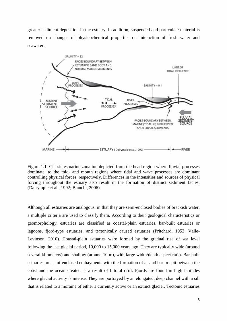
greater sediment deposition in the estuary. In addition, suspended and particulate material is
removed on changes of physicochemical properties on interaction of fresh water and
seawater.
Figure 1.1: Classic estuarine zonation depicted from the head region where fluvial processes
dominate, to the mid- and mouth regions where tidal and wave processes are dominant
controlling physical forces, respectively. Differences in the intensities and sources of physical
forcing throughout the estuary also result in the formation of distinct sediment facies.
(Dalrymple et al., 1992; Bianchi, 2006)
Although all estuaries are analogous, in that they are semi-enclosed bodies of brackish water,
a multiple criteria are used to classify them. According to their geological characteristics or
geomorphology, estuaries are classified as coastal-plain estuaries, bar-built estuaries or
lagoons, fjord-type estuaries, and tectonically caused estuaries (Pritchard, 1952; Valle-
Levinson, 2010). Coastal-plain estuaries were formed by the gradual rise of sea level
following the last glacial period, 10,000 to 15,000 years ago. They are typically wide (around
several kilometers) and shallow (around 10 m), with large width/depth aspect ratio. Bar-built
estuaries are semi-enclosed embayments with the formation of a sand bar or spit between the
coast and the ocean created as a result of littoral drift. Fjords are found in high latitudes
where glacial activity is intense. They are portrayed by an elongated, deep channel with a sill
that is related to a moraine of either a currently active or an extinct glacier. Tectonic estuaries

4
were formed by earthquakes and fractures of the Earth’s crust that generated faults in the
regions near the ocean, causing the crust to sink and form a hollow basin that is filled by the
ocean.
Further, based on stratification and circulation, estuaries have also been classified as salt
wedge estuaries, vertically homogeneous estuaries and partially mixed estuaries. A salt-
wedge estuary is highly stratified and has minimal mixing wherein the seawater forms a
wedge, thickest at the seaward end, tapering to a very thin layer at the landward limit. The
vertically homogenous estuary occurs when the river flow is low and strong tidal currents
eliminate the vertical layering of fresh water floating above denser seawater. The saline water
and fresh water tend to mix vertically, and at times laterally as well. Intermediate estuaries
are partially mixed and exhibit circulation patterns that are somewhere between the salt-
wedge and vertically homogenous estuaries wherein the deeper water layers remain more
saline than the upper layers.
On the basis of water balance, estuaries are classified into three types: positive, inverse and
low-in flow estuaries. In positive estuaries, freshwater additions from river discharge, rain
and melting ice exceed freshwater losses from evaporation or freezing and a longitudinal
density gradient established. Inverse estuaries are found in arid regions where loss of
freshwater from evaporation exceeds freshwater additions from precipitation and the river
discharge scarce into these systems. Low-inflow estuaries also occur in regions with high
evaporation rates but with a small influence from river discharge.
Based on tidal range, Hayes (1975) defined three types of estuaries: microtidal, mesotidal and
macrotidal estuaries. Microtidal estuaries have a tidal range less than 2 m and are dominate
by wind and wave action. The principal forms of deposition are river and flood deltas, wave
built features such as spits, bars, beaches, and storm deposits. Mesotidal estuaries have a tidal
range between 2 m and 4 m. Macrotidal estuaries have a tidal range greater than 4 m and are
generally have a broad and funnel shaped mouth with linear sand bodies occupying the
central portion and extensive tidal flats and salt marshes bordering the coasts
Estuaries contain many different habitats such as shallow open waters, sandy beaches, salt
marshes mud and sand flats, rocky shores, mangrove forests, seagrass beds, river deltas and
tidal pools. Out of these, mangrove and mudflats have received considerable attention as they

5
are very effective in coastal protection, respond to sea level changes and offer an important
habitat for wildlife, food and recreation.
Mangroves are a diverse group of trees, palms, shrubs, vines and ferns that have the ability to
thrive in waterlogged saline soils that are subjected to regular flooding by tides. The global
mangrove area is estimated to cover l00000 km2 to 230000 km
2 of sheltered coastal intertidal
land which is <0.2% of the global land surface area (Bunt, 1992; Snedaker, 1984; Jennerjahn
and Ittekkot, 1997) and accounts for approximately 75% of coastal vegetation (Linden and
Jernelov, 1980). They are highly specialized plants that have developed specialized
adaptations to the unique environmental conditions in which they are found. Mangrove
forests are typically found in the tropical and sub-tropical latitudes, lying between the land
and the sea in sheltered coastal areas that are subjected to tidal influence and are among the
most productive ecosystems (Kathiresan and Bingham, 2001; Kathiresan, 2002). The
mangrove ecosystems play an important role in carbon, nitrogen, phosphorus, and sulfur
cycles, in addition to providing protection to coastal areas from waves and storms (Meng et
al., 2016). Mangroves are known for being sites for sediment deposition and are associated
carbon and nutrients (Eyre, 1993; Furukawa and Wolanski, 1996). The mangroves trap
sediment by their complex aerial root structure and are an important sink for suspended
sediments and thus function as land builders (Woodroffe, 1992; Wolanski et al., 1992;
Wolanski 1994, 1995; Furukawa et al., 1997). Mangroves tend to accelerate the
sedimentation process with the annual sedimentation rate in mangroves ranging from 1 to
8 mm (Bird and Barson, l977; Woodroffe, l992). In addition, they are vital habitats for
aquatic organisms, birds and other terrestrial animals. The mangrove trees supply large
amounts of organic matter, which is consumed by many small aquatic animals. These
organisms provide food for larger fish and other animals. Mangroves also help to maintain
water quality by filtering the silt from runoff and recycling nutrients.
Mudflats are coastal wetlands formed in sheltered shores where greater amounts of
sediments, detritus are deposited by the rivers or tides. They are frequently associated with
estuaries, and are usually situated adjacent to mangroves and comprise around 7 % of total
coastal shelf areas (Stutz and Pikey, 2002). Intertidal mudflats play a critical role in the
estuarine exchange of marine and continental supplies of nutrients and sediments. The
mudflat habitat represents a transition from subtidal sediment areas that are successively
flooded and uncovered by tides and/ or river discharge variations (Deloffre et al., 2005,

6
2007). Mudflats are the interface between the flood plain and the main river channel, and are
characterized by a cross-shore slope typically separated into two specific environments: the
shore in the upper part of the mudflat that flooded during high spring tides; and the tidal flat
that is the lower part of the mudflat and has an upper limit corresponding to the highest sea
level reached during the mean tidal range (Jaud et al., 2016). The sediments consist mainly
of fine particles, mostly in the silt and clay fraction. Little oxygen penetrates through the
cohesive sediments, and an anoxic layer is often present within millimeters of the
sediment surface. Mudflats generally support very little vegetation other than green algae.
Their biodiversity centers on the range of invertebrates living in the sediment which are
biologically productive. The intertidal mudflats support communities characterized by
polychaetes, bivalves and oligochaetes and large numbers of birds and fish. Mudflats
provide an important nursery and feeding ground for many fish species.
The characteristics of an estuary are determined by the dynamics of various processes and the
sediment sources. Material is imported from the river and its catchments, and sea into the
estuary where the transformation of material takes place. Post transformation, a part of the
material such as a particulate matter is retained in the estuary in sediments whereas the
dissolved material is exported to the sea (Turner and Riddle, 2001). The main sediment
sources of an estuary are from existing base material, terrigenous material held in the
catchment and sand transported from the open-coast marine environment. In addition
particulate and dissolved matter composed of organic and inorganic material is added in to
the estuary that may be supplied naturally or from anthropogenic sources. The distribution of
the sediments within an estuary is regulated by interactions between the available sediments,
bottom morphology and flow hydrodynamics (Frey and Howard, 1986). The dynamics of
sediment transport depend on the water circulation, salinity, biological interaction, and
sediment type (Wang and Andutta, 2013). The interaction among cohesive sediments (mud)
is different from that of non-cohesive sediments (sand). Cohesive sediments may aggregate,
forming flocs by the flocculation process caused by chemical or biological interaction.
Flocculation increases the settling velocity of sediment particles. Chemical flocculation is
started by salinity, ions that attach to the small mud particles, cause electronic forces between
the particles, which start aggregating and thus forming a larger mud floc. In contrast,
“Biological flocculation” is caused by bacteria and plankton that produce exopolymer and
binds mud particles leading to formation of extremely large flocs of ~1000 µm in size
(Wolanski et al., 2012).
7
Sediments that are transported by the estuarine waters typically cover a range of sizes
from less than 0.002 mm to more than 4 mm, with the finer sizes dominant in most estuaries.
Estuarine sand is typically composed of quartz, although other minerals such as feldspar or
various heavy minerals such as magnetite may be present depending on the sediment
source. The fine sediments in estuaries are mixtures of inorganic minerals, organic materials,
and biochemicals. Mineral grains usually consist of clays such as montmorillonite, illite, and
kaolinite and chlorite, and non-clay minerals like quartz and carbonate. Organic materials
comprise of biogenic detritus and microorganisms (McNally and Mehta, 2004).
The estuarine system is mainly an area of deposition and acts as an important sink for metals
in the environment. Metals are supplied to the estuary by natural factors such as chemical
leaching of bedrocks, water drainage basins, and runoff from banks while the discharge of
urban and industrial waste water, combustion of fossil fuels, mining and smelting operations,
waste disposal and transportation activities are the important anthropogenic sources of the
metal pollutants (Abdullah et al., 1999; Shazili et al., 2006; Dragun et al., 2009; Pardo et al.,
1990; Zhou et al., 2008). Metals brought into the estuary are transferred from solution to
sediments by adsorption onto suspended particulate matter, and are deposited with relatively
short lag times and tend to get trapped and accumulate in the sediments (Spencer et al.,
2003). The distribution and accumulation of metals are influenced by the sediment texture,
mineralogical components and physical transport (Buccolieri et al., 2006; Marchand et al.,
2006). The metals get assimilated in the sediment along with organic matter, Fe/Mn oxides,
sulphide, and clay and thus undergo alterations in their speciation due to geochemical
modifications by processes such as dissolution, precipitation, sorption and complexation
when discharged into the estuary and form several reactive components (Lim et al., 2012).
The sediment characteristics such as pH, cation exchange capacity, organic matter content,
redox conditions, chloride content and salinity determine metal sorption and precipitation
processes, which are associated to the metal mobility, bioavailability and potential toxicity
(Du Laing et al., 2002). The organic matter content in the sediments leads to relatively higher
metal accumulation (Zhong et al., 2006). In addition, sediment grain size substantially
influences the metal concentration in the estuarine sediments as the clay fractions that have a
high specific surface area, favor adsorption processes (Thuy et al., 2000). Following
deposition and burial, metals become subject to a variety of physical, chemical and biological
processes which may mix and remobilize the metals into the water column (Lee and Cundy,

8
2001) or may be immobilized in the sediments for long periods of time and undergo
compaction and diagenesis.
The chemical speciation of metals in sediments involves the identification and quantification
of the different forms or phases of the metal present in the sediments and provides advanced
information on the potential availability of metals to biota under various environmental
conditions (Álvarez-Iglesias and Rubio, 2009; Fytianos and Lourantou, 2004; Gao et al.,
2008; Rauret et al., 1998). The fractionation procedure can indicate the propensity for metals
to be remobilized and can help distinguish those metals having a lithogenic origin from those
with an anthropogenic origin (Förstner et al., 1990; Korfali and Jurdi, 2011). Tessier et al.
(1979) devised a fractionation procedure which defined the desired partitioning of trace
metals into fractions that are likely to be affected by various environmental conditions i.e.
exchangeable, bound to carbonates, bound to iron and manganese oxides, organic
matter/sulfide bound and the residual fraction. The metals in the exchangeable fraction are
likely to be affected by sorption-desorption processes such as weakly bound to clays,
hydrated oxides of iron and manganese and humic acids while the metals in the carbonate
fractions can be associated with sediment carbonates and this fraction is susceptible to
changes of pH. Together the exchangeable and carbonate fractions are known as the labile
fraction (Perin et al., 1985). The third fraction of sediment consists of metals bound to iron
and manganese oxides and these oxides are excellent scavengers for trace metals (Gutierrez,
2000) and are thermodynamically unstable under anoxic conditions. The fourth fraction
consists of trace metals bound to various forms of organic matter such as detritus, humic and
fulvic acids etc, through complexation and peptization phenomenon. A large amount of
sulfides are also leached into this fraction. Under oxidizing conditions in natural waters, the
degradation of organic matter leads to the release of soluble trace metals. The residual
fraction of the sediments consists of primary and secondary minerals which may retain trace
metals within their crystal structure and are not released easily into solution. The first four
fractions are known as the bioavailable fraction as they exhibit mobility and are potentially
available for uptake by organisms. The mobile fractions introduced by anthropogenic
activities remain bound to the exchangeable, the carbonate and the easily reducible phases
(Nair, 1992). The sediment-associated metals have the potential to be ecotoxic due to their
mobility and bioavailability, and this in turn affects both ecosystems and life through a
process of bioaccumulation and biomagnification, respectively (Buccolieri et al., 2006; Ip et
al., 2007). Thus, evaluating metal speciation can provide detailed information about the

9
origin, mobilization, contamination risks, biological availability and toxicity of metals (Yang
et al., 2014).
As sediments are often the final repository of metals, accumulation of high concentrations of
metals can present a risk to organisms (Casado-Martinez et al., 2013). Metals normally
occurring in nature are not harmful to the environment, because they play an essential role in
tissue metabolism and growth of plants and animals (Amundsen et al., 1997). However,
metals like Cu, Zn, Fe, Co, Mo, Ni, Si, and Sn become predominantly toxic when their level
exceeds the limit, and V, Cd, Pb, and Hg are prominently classified as toxic because of their
detrimental effect even at low concentrations (Michael, 2010). Marine organisms can
accumulate metals in their tissues that may threaten the health of organisms higher in the
food chain through trophic transfer to terrestrial, estuarine and eventually coastal species that
become prey for oceanic predators and humans (Boyle et al., 2008; Cheung and Wang, 2008).
Metals are ingested of metal-enriched sediment and suspended particles during feeding, and
by uptake from solution (Luoma, 1983). The ecological risk posed by metal-contaminated
sediments depends strongly on the sediment characteristics, specific chemical forms of the
metals, influencing their availability to aquatic organisms (bioavailability) and the ability of
these organisms to accumulate (bioaccumulation) or remove metals. The efficiency of
bioaccumulation via sediment ingestion is dependent on geochemical characteristics of the
sediment. Various accumulation patterns have been described regulating the uptake of metals
defined by the balance between uptake and excretion rates (Luoma et al., 2008; Rainbow,
2002) and by detoxification processes usually involving proteins such as metallothioneins
(Casado – Martinez et al., 2010; Greim and Snyder, 2008; Walker et al., 2012).
Thus, the analysis of estuarine sediments offers certain advantages. The surface sediment
often exchanges with suspended materials, thereby affecting the release of metals to the
overlying water (Zvinowanda et al., 2009). As a result, the top few centimeters of the
sediments reflect the continuously changing present-day degree of contamination, whereas
the bottom sediments record its history (Seshan et al., 2010). Therefore, the metal
concentration in sediment core profiles give information on the weathering processes and
post- depositional mobility of metals (Subramanian and Mohanchandran, 1994).

10
1.2 Literature review
Table 1.1 Literature survey of the research studies carried out of late in India and other
regions of the world
Authors Parameters
analyzed
Observations
Prajith et al.,
2016
Grain size, organic
carbon, major
elements and trace
metals, speciation
of metals
Major elements and trace metals were analyzed in
sediment cores of the Mandovi estuary to
investigate their distribution, provenance and early
diagenesis. The results showed that the sediment
texture ranged from clayey silts to sand-dominated
sediments and the organic carbon content was
higher in fine-grained sediments. The contribution
metals Ti, V, Cr and Zr to the sediments were
probably from the laterites of the hinterland and
abundant Fe and Mn in the estuary were due to the
anthropogenic activities on the shore. The trace
metals were redistributed in the organic-rich
sediments due to early diagenetic processes. In
addition, the sediments showed significant pollution
by Mn and Cr and the high Mn content is
susceptible to be mobilized along with redox-
sensitive metals under reducing conditions.
Prajith et al.,
2015
Grain size, organic
carbon, magnetic
parameters, Fe and
Mn
The magnetic properties of sediments were
examined in 7 gravity cores that were collected
along transect of the Mandovi estuary, to
understand sediment provenance and pollution. The
magnetic parameters indicated that hematite and
goethite dominated in the sediments of the
upper/middle estuary and magnetite-dominated in
the sediments of the lower estuary/bay and the two
sediment types were discernible because of the

11
deposition of abundant ore material in the
upper/middle estuary whereas detrital sediment
were deposited in the lower estuary/bay. The
enrichment factor and the index of geo-
accumulation of metals indicated significant to
strong pollution by Fe and Mn in the upper/middle
estuary.
Kessarkar et al.,
2015
Magnetic
parameters
The environmental magnetic properties of
sediments of the Mandovi and Zuari estuaries and
the adjacent shelf were investigated. The study
revealed that the magnetic susceptibility (χlf) and
saturation isothermal remanent magnetization
(SIRM) values of sediments were highest in
upstream and, decreased gradually towards the
downstream region of the estuary and were lowest
on the adjacent shelf. The χlf values of the Mandovi
estuary were two to four folds higher than those in
the Zuari. In addition, the sediments of these two
estuaries showed the enrichment of older magnetite
after the mining ban.
Rao et al., 2015
Grain size, clay
minerals, Sr- Nd
isotopes
The clay mineralogy and Sr-Nd isotopes of the
suspended particulate matter (SPM) and the bottom
sediments in the Mandovi and Zuari estuaries were
investigated to determine the provenance and role
of estuarine processes on their distribution. It was
reported that kaolinite and illite followed by minor
gibbsite, goethite and chlorite are the intense
chemical weathering products of the laterites in the
hinterland whereas smectite may have formed in the
coastal plains. The high 87
Sr/86
Sr ratios at river end
stations of both estuaries indicated intense chemical
weathering of the hinterland laterites while the ƐNd

12
values indicated the influence of lateritic weathering
and anthropogenic contribution of ore material to
the SPM and the bottom sediments of both the
estuaries.
Venkatramanan
et al., 2015
Salinity, grain size,
organic matter,
speciation of
metals in
sediments
A study was carried out to estimate the
concentrations of the metals Fe, Mn, Cr, Cu, Co, Ni,
Pb and Zn in surface sediments from the
Tirumalairajan river estuary with an aim to
investigate their speciation, the effects of grain size,
physico-chemical parameters and organic matter, to
trace the metal source and to understand the
seasonal variation and the geochemical
accumulative phase of the metals. The results
revealed that metals were higher in the residual
fraction and were thus derived mainly from
geogenic origin in addition to minor contribution
from anthropogenic origin. The fine sediments and
organic matter acted as efficient scavengers for
metals and the metal concentrations posed a low
environmental risk.
Kumar and
Ramanathan,
2015
Grain size,
speciation of
metals
The study was conducted to highlight the
distribution of trace metals in the mangrove
sediments of the Sundarbans in India and
Bangladesh using a speciation technique to
document the bioavailability and the environmental
hazards associated with the operationally defined
chemical forms of trace metals. The results
indicated the dominance of anthropogenic activity
and the lack of freshwater flow affected the
speciation profile of trace metals in the mangrove
sediments.

13
Birch et al., 2015 Fine nutritive
roots, leaves and
pneumatophores,
metals
The study was carried out to determine the
remediation effectiveness of a former Pb-
contaminated industrial site in Homebush Bay in
the Sydney estuary (Australia) through the sampling
of intertidal sediments and mangrove (Avicennia
marina) tissues (fine nutritive roots,
pneumatophores, and leaves). The results indicated
that since remediation carried out 6 years ago, the
metal concentrations in the surficial sediment have
increased which may have been sourced either from
the surface/ subsurface water from the catchment or
more likely the remobilized contaminated sediments
from the un-remediated regions. The results also
indicated that with increasing surficial sediment
metal concentrations, the metal levels in mangrove
tissue are likely to increase over time.
Fernandes and
Nayak, 2015
Grain size, organic
carbon, speciation
of metals
Sediment cores collected from mudflat
environments of the Swarna and Gurpur estuaries,
India were studied to understand the bioavailability
of metals in sediments and their probable toxicity.
Most trace metals in both the cores were mainly
from lithogenic source and the metal speciation
indicated that Mn, Ni, Cu and Co concentrations in
Gurpur estuary indicated anthropogenic additions in
recent years whereas in Swarna estuary most metals
exhibited diagenetic remobilization and diffusion to
the water column from surface sediments.
Veerasingam et
al., 2015
Grain size, trace
metals, scanning
electron
microscopy
The concentrations of trace metals (Fe, Mn, Cu, Cr,
Co, Pb and Zn) in three sediment cores were
analyzed to assess the depositional trends of metals
and their respective contamination levels in the
Mandovi estuary, west coast of India. The

14
enrichment of trace metals suggested an excess of
anthropogenic loadings (including mining activities)
occurred lately. Scanning electron microscope
images of core sediments distinguished the shape,
size and structure of particles derived from
lithogenic and anthropogenic sources. The geo-
accumulation index (Igeo) values indicated that
Mandovi estuary sediments are ‘moderately
polluted’ with Pb, and ‘unpolluted to moderately
polluted’ with Fe, Mn, Cu, Cr, Co and Zn.
da Silva et al.,
2014
Grain size, cation
exchange capacity,
organic matter, pH,
speciation of
metals in
sediments
The study was carried out on mangrove sediments
of the Tibiri River Estuary, Brazil to evaluate the
three geochemical fractions of trace metals (Cd, Cr,
Cu, Ni, Pb and Zn) in sediments i.e. the
exchangeable/acid-soluble, reducible and oxidizable
fractions and to assess the risks of trace metals
using the TEL/PEL and ERL/ERM guide values for
the protection of the aquatic life. The results
demonstrated that metal levels were below TEL
(Threshold effect level) and ERL (effect range low)
ranges and was associated with occasional adverse
biological effects for the aquatic life.
He et al., 2014 Mangrove leaves
and stems, metals
Heavy metals in mangrove sediments and plants
were assessed in the Futian mangrove forest of
Shenzhen, China to evaluate the characteristics of
heavy metal contamination, that included essential
elements (Cu and Zn) and non-essential elements
(Cr, Ni, As, Cd, Pb and Hg). The results indicated
that the heavy metals Cd, As, Pb and Hg contents
were higher than the background values in
sediments while in mangrove plants’ leaves and
stems, concentrations of Cu, Zn and As were

15
higher. The high heavy metal concentrations in
sediments and low levels in leaves and stems
indicated that mangrove plants actively avoided the
uptake of heavy metals even when sediment metal
concentrations are high. The high bioconcentration
factors for Cr implied its potential use as a temporal
Cr contamination indicator in sediments.
Chakraborty et
al., 2014 (a)
Sediment grain
size, total carbon,
total nitrogen,
metals in
mangrove
sediments and
roots, kinetic
speciation of Ni
and Cu in the
mangrove
sediments
Kinetic speciation study was carried out to
determine the concentrations of labile metal-
complexes and their dissociation rate constants in
the mangrove sediments of the Divar Island in Goa,
India to establish a linkage between chemical
speciation of copper and nickel and their
bioavailability in the mangrove ecosystem.
It was found that the bioaccumulation of both the
metals gradually increased with the increase in
concentrations of the labile metal complexes and
their dissociation rate constants in the mangrove
sediments. In addition, the concentration of labile
metal complexes and their dissociation rate
constants in mangrove sediment can be a useful
indicator of their bioavailability.
Chakraborty et
al., 2014 (b)
Metals in
sediments
This review comprehended the changes in metal
contamination levels with time in surface estuarine
sediments around India. This study indicated that
estuarine sediments from the east coast of India
were comparatively less contaminated by metals
than the west coast. In addition, the sediments of
estuaries that were located near major cities were
found to be more contaminated by metals. An
improvement in estuarine sediment quality over
time around India was noted.
16
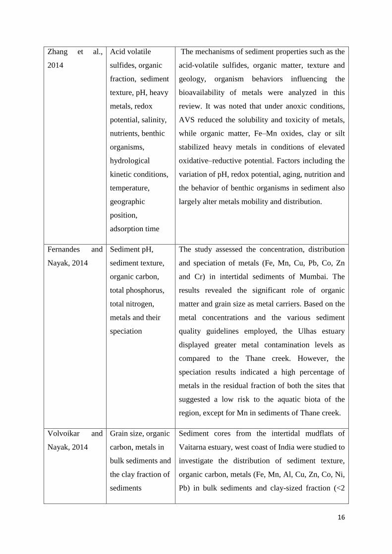
Zhang et al.,
2014
Acid volatile
sulfides, organic
fraction, sediment
texture, pH, heavy
metals, redox
potential, salinity,
nutrients, benthic
organisms,
hydrological
kinetic conditions,
temperature,
geographic
position,
adsorption time
The mechanisms of sediment properties such as the
acid-volatile sulfides, organic matter, texture and
geology, organism behaviors influencing the
bioavailability of metals were analyzed in this
review. It was noted that under anoxic conditions,
AVS reduced the solubility and toxicity of metals,
while organic matter, Fe–Mn oxides, clay or silt
stabilized heavy metals in conditions of elevated
oxidative–reductive potential. Factors including the
variation of pH, redox potential, aging, nutrition and
the behavior of benthic organisms in sediment also
largely alter metals mobility and distribution.
Fernandes and
Nayak, 2014
Sediment pH,
sediment texture,
organic carbon,
total phosphorus,
total nitrogen,
metals and their
speciation
The study assessed the concentration, distribution
and speciation of metals (Fe, Mn, Cu, Pb, Co, Zn
and Cr) in intertidal sediments of Mumbai. The
results revealed the significant role of organic
matter and grain size as metal carriers. Based on the
metal concentrations and the various sediment
quality guidelines employed, the Ulhas estuary
displayed greater metal contamination levels as
compared to the Thane creek. However, the
speciation results indicated a high percentage of
metals in the residual fraction of both the sites that
suggested a low risk to the aquatic biota of the
region, except for Mn in sediments of Thane creek.
Volvoikar and
Nayak, 2014
Grain size, organic
carbon, metals in
bulk sediments and
the clay fraction of
sediments
Sediment cores from the intertidal mudflats of
Vaitarna estuary, west coast of India were studied to
investigate the distribution of sediment texture,
organic carbon, metals (Fe, Mn, Al, Cu, Zn, Co, Ni,
Pb) in bulk sediments and clay-sized fraction (<2

17
microns). The results demonstrated that Fe-Mn oxy-
hydroxides controlled the distribution of most
metals in the core collected towards the lower
middle estuary and the mouth. The greater
deposition of metals in the clay fraction in recent
times was due to increased marine inundation that
caused greater flocculation and deposition of metals
and finer clay particles. The metals associated with
the clay fraction were least affected by
anthropogenic activities while the metals that
showed enrichment in the bulk sediments implied
the association of metals with the coarser sediment
particles and Fe-Mn oxy-hydroxides, thus
indicating their anthropogenic additions along with
lithogenic inputs.
Kathiresan et al.,
2014
Metals in
sediments,
mangrove bark,
root and leaves
The study was carried out to analyze the
concentrations of 12 micro-nutrients (Al, B, Cd, Co,
Cr, Cu, Fe, Mg, Mn, Ni, Pb, and Zn) in various
plant parts of Avicennia marina and its rhizosphere
soil of the south east coast of India. The sediments
held more levels of metals than plant parts, but
within the permissible limits of concentration. The
bark and root accumulated higher concentrations of
trace elements than other plant parts. The essential
elements accumulated in higher concentrations in
mature mangrove forest while non-essential
elements accumulated high metal concentrations in
the industrially polluted mangroves.
Birch et al., 2014 Oyster tissue,
metals, sediments,
SPM
The study aimed to deduce the relationship between
metals in sediments and metal bioaccumulation in
oyster tissues in the Sydney estuary, Australia. The
SPM and surficial sediment contained high Cu, Pb

18
and Zn concentration. The oyster tissue metal
content varied greatly at a single locality over
temporal scales of years. The Oyster tissue was
found to exceed consumption levels for Cu. It was
proposed that the bioaccumulation of metals in
oyster tissue is a useful indicator of anthropogenic
influence in estuaries.
Nath et al., 2014 Metals in
sediments,
pneumatophores,
bioavailability
Heavy metal concentrations in pneumatophore
tissues and ambient sediments from Sydney
Estuary, Australia were investigated to assess the
bio-indication potential of Avicennia marina. The
results indicated that the metal concentrations in
sediment were mostly above the Australian interim
sediment quality guidelines and the enrichment
factors indicated “very severe” modification of
sediment. High bioconcentration factors were
observed for Cu and Ni in comparison with other
metals (As, Cd, Co, Cr, Pb and Zn). In addition, a
strong, positive relationship between metals in
sediments and pneumatophores suggested the
potential use of these tissues as a bio-indicator of
estuarine contamination and that metals are entering
the biotic environment. The study further
highlighted the positive role of mangroves in metal
sequestration from sediments and the water column
and thus protecting the estuarine environments from
pollution.
Kesavan et al.,
2013
Metals in
sediments, shells
and tissues of
molluscs.
The concentration of metals (Cd, Co, Cu, Fe, Mg,
Mn, Pb, Zn) were analyzed in sediments, shells and
tissues of molluscs i.e. Meretrix meretrix,
Crassostrea madrasensis and Cerithidea cingulata
from the Uppanar Estuary, southeast coast of India.

19
The results demonstrated that the concentrations of
the heavy metals analyzed exhibited spatial
variations in sediments, tissues and shells. The
concentration of heavy metals in the tissue was
higher than the shell. Furthermore, it was proposed
that oysters are particularly recommended as
biomonitors over bivalves, due to their strong
accumulation patterns for many metals, their large
size and their local abundance whereas the bivalves
assimilate metals from solution and suspended
material.
Shynu et al.,
2013
Suspended
particulate matter,
salinity, rare earth
elements, major
elements
The concentrations of Al, Fe, Mn and rare earth
elements (REE) were measured in suspended
particulate matter (SPM) and surficial sediments
from the Zuari estuary and the adjacent shelf to
understand their distribution, provenance and
estuarine processes. The results indicated that the
REE of SPM/sediment is dominated by Fe, Mn ore
dust and, its distribution along transect is influenced
by the estuarine turbidity maximum (ETM). The
ETM and seasonal circulation in the estuary
controlled the mixing and the advective transport of
particulates to the shelf during monsoon and into
the estuary during dry season. This study indicated
that the sediment contribution to the shelf from
tropical, minor rivers is controlled by the
hydrodynamic conditions in the estuaries.
Singh et al.,
2013
Grain size, organic
carbon, major
elements and
metals
This study presented the variation in sediment
components and metal distributions between three
cores collected from three mudflats of the Zuari
estuary. The cores collected from upper middle
estuarine mudflats showed higher values of finer

20
fractions, TOC and metals, than the core collected
near the river mouth. Mn, Ca, and to some extent
with Fe and Zn in sediments were likely of local
anthropogenic inputs. Overall, the highest
concentrations of metals were found in the upper
middle estuarine mudflats and may be attributed to
the nearby mining zone and the transportation of ore
by barges in these water courses. In the lower
estuarine core, the diagenetic signal was masked by
the high input of Fe and Mn. The enrichment factors
revealed a high degree of metal contamination in
sediments.
Rumisha et al.,
2012
Organic matter,
sediments grain
size, metal analysis
in sediments and
molluscan tissues
The effects of trace metal pollution on the
community structure of soft bottom molluscs were
investigated in intertidal areas of the Dar es Salaam
coast, Tanzania. The result revealed that the
community structure of the soft bottom molluscs
along the Dar es Salaam coast was influenced by
trace metals pollution. The soft bottom molluscs
exhibited species-specific responses to specific
contaminants wherein the gastropods L. aberrans,
A. fortis and A. ovata were very sensitive to trace
metals pollution whereas the gastropod M. honkeri
was tolerant to As and other trace metals. The study
also revealed that soft bottom molluscs exhibited
species-specific responses to specific contaminants
due to the different capabilities in accumulating and
regulating toxicants.
Palpandi and
Kesavan, 2012
Metals in
sediments and
gastropod shell and
tissue.
The objective of the study was to estimate the
levels of the metals Fe, Al, Mg, Mn, Cd, Cu, Pb,
Zn, Cr and Ni in mangrove sediments of the Vellar
estuary, Southeast coast of India and shells and soft
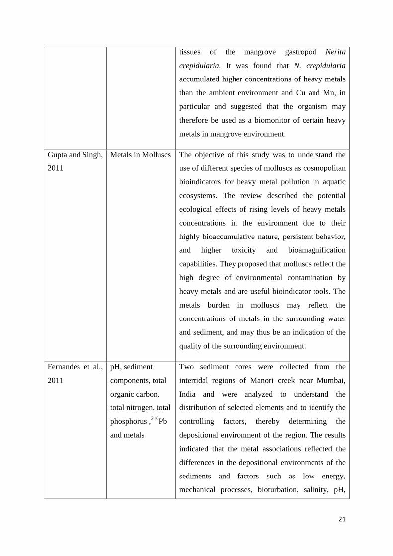
21
tissues of the mangrove gastropod Nerita
crepidularia. It was found that N. crepidularia
accumulated higher concentrations of heavy metals
than the ambient environment and Cu and Mn, in
particular and suggested that the organism may
therefore be used as a biomonitor of certain heavy
metals in mangrove environment.
Gupta and Singh,
2011
Metals in Molluscs The objective of this study was to understand the
use of different species of molluscs as cosmopolitan
bioindicators for heavy metal pollution in aquatic
ecosystems. The review described the potential
ecological effects of rising levels of heavy metals
concentrations in the environment due to their
highly bioaccumulative nature, persistent behavior,
and higher toxicity and bioamagnification
capabilities. They proposed that molluscs reflect the
high degree of environmental contamination by
heavy metals and are useful bioindicator tools. The
metals burden in molluscs may reflect the
concentrations of metals in the surrounding water
and sediment, and may thus be an indication of the
quality of the surrounding environment.
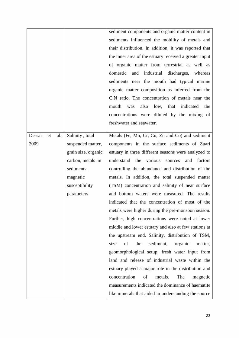
Fernandes et al.,
2011
pH, sediment
components, total
organic carbon,
total nitrogen, total
phosphorus ,210
Pb
and metals
Two sediment cores were collected from the
intertidal regions of Manori creek near Mumbai,
India and were analyzed to understand the
distribution of selected elements and to identify the
controlling factors, thereby determining the
depositional environment of the region. The results
indicated that the metal associations reflected the
differences in the depositional environments of the
sediments and factors such as low energy,
mechanical processes, bioturbation, salinity, pH,
22
sediment components and organic matter content in
sediments influenced the mobility of metals and
their distribution. In addition, it was reported that
the inner area of the estuary received a greater input
of organic matter from terrestrial as well as
domestic and industrial discharges, whereas
sediments near the mouth had typical marine
organic matter composition as inferred from the
C:N ratio. The concentration of metals near the
mouth was also low, that indicated the
concentrations were diluted by the mixing of
freshwater and seawater.
Dessai et al.,
2009
Salinity , total
suspended matter,
grain size, organic
carbon, metals in
sediments,
magnetic
susceptibility
parameters
Metals (Fe, Mn, Cr, Cu, Zn and Co) and sediment
components in the surface sediments of Zuari
estuary in three different seasons were analyzed to
understand the various sources and factors
controlling the abundance and distribution of the
metals. In addition, the total suspended matter
(TSM) concentration and salinity of near surface
and bottom waters were measured. The results
indicated that the concentration of most of the
metals were higher during the pre-monsoon season.
Further, high concentrations were noted at lower
middle and lower estuary and also at few stations at
the upstream end. Salinity, distribution of TSM,
size of the sediment, organic matter,
geomorphological setup, fresh water input from
land and release of industrial waste within the
estuary played a major role in the distribution and
concentration of metals. The magnetic
measurements indicated the dominance of haematite
like minerals that aided in understanding the source

23
and depositional processes.
Dessai and
Nayak, 2009
Grain size, organic
carbon, bulk
metals and
speciation of
metals in
sediments.
Surface sediments from Zuari estuary, Goa were
analyzed by a sequential procedure for metals Fe,
Mn, Cu, Zn, Cr and Co to determine their
distribution the in five geochemical phases. The
total metal content, sand, silt, clay and organic
carbon were also determined of the surface
sediments. The results indicated an enrichment of
metals probably due to anthropogenic inputs. The
results obtained from the sequential procedure
showed that Mn and Co were potentially
bioavailable indicating their importance in toxicity
whereas metals Fe, Cu, Zn and Cr were high in the
residual phase. Further, it was reported that the
main source of metals to the estuary was mining
and its associated activities in the study area.
1.3 Objectives
Earlier studies have focused on the sediment distribution, transport and geochemistry within
the estuarine channel using suspended particulate matter, surface sediments and mudflat cores
of the Zuari estuary. Further research is necessary to provide information on the distribution
of metals and their speciation in the sediment to understand the deposition, migration and
accumulation mechanisms, their bioavailability, bioaccumulation and toxicity to organisms
associated with the sediments. Therefore, a comprehensive multi proxy approach analysis
was carried out to understand the processes occurring in the estuary, specifically in the
mangroves and mudflats as these depositional environments are sinks as well as sources for
many metals, natural as well as anthropogenic. The present study was carried out along
transect of the Zuari estuary with the following objectives:
1. To study the abundance and distribution of metals in sediments and to understand the role
of physicochemical and geochemical parameters influencing the distribution of metals.

24
2. To study the concentration of metals in soft tissue of selected biota associated with
sediments.
3. To establish a relation between bioavailability of metals in sediments and bioaccumulation
of metals in biota.
1.4 Study area
The Zuari estuary is located on the west coast of India, is classified as a tide-dominated,
coastal plain estuary and geomorphologically as drowned river valley estuary (Murty et al.,
1976). The estuary has a basin area of 973 km2, catchment area of around 550 km
2 and tidal
range of 2.3 (Singh et al., 2013) with surface run off of 2247.4 MCM (Kessarkar et al., 2015).
The Zuari River originates in Hemad– Barshem in the Western Ghats and is about 70 km in
length. The hinterland of Zuari is covered by rocks of the Dharwar Super Group of the
Archaean Proterozoic age represented by metamorphosed basic and acid volcanic rocks and
sediments at the base, overlain by greywacke suite of rocks, which in turn, is followed by
pyroclasts and tuffs with the associated chaemogenic precipitates of lime, manganese and
iron and again overlain by greywacke suite of rocks (Gokul et al., 1985; Dessai et al., 2009).
Most of these formations have been lateritized, with original unweathered rocks exposed only
in coastal headlands, along steep slopes of high hills or in manmade cuttings like quarries,
road cuts, and railway tunnels (Fernandes, 2009) The hinterland rocks of the Zuari estuary are
subjected to intense chemical weathering under humid tropical climate conditions. Two
thirds of the area in Goa is covered by laterite (Nayak, 2002), that has been formed after
extensive leaching of other elements and due to the concentration of iron and aluminum.
Alluvial and loamy soils are found along the riverbanks and are rich in minerals and humus.
River flow dominates during monsoon, but in the remaining period, tidal flow dominates and
the lower estuary becomes an extension of the sea (Shetye et al., 2007). The Cumbharjua
canal of length around 17 km connects the Mandovi and Zuari at distances of 14 and 11 km,
respectively, from their mouths. The catchment areas of the adjacent Mandovi and the Zuari
estuaries are known for open cast mining of ferromanganese ores. The mined ore is stored in
stacks on the river banks for loading onto barges that transport the ores to the Mormugao
harbor located at the southern bank of the Zuari and loaded onto larger ships. Around 15
million tons of iron and manganese ore was transported annually along these rivers to the

25
nearby Mormugao harbor in 1990’s (Satyanarayana and Sen Gupta, 1996) which increased to
around 50 million tons in 2010’s. The ore stored for transportation at different points on the
shores of the estuary gets eroded and flushed into the estuaries during heavy monsoon rains
and part of the ore and/or dust ultimately gets accumulated in the estuaries and is
incorporated into sediments (Shynu et al., 2012; Alagarsamy, 2006; Dessai et al., 2009). The
Cumbharjua canal adds much of the mining material to the Zuari during the monsoons and
ebb tide (Dessai and Nayak, 2009). Iron ore was mined from the banded iron formations of
Goa, India, and transported through the Mandovi and Zuari estuaries for six decades until the
ban on mining from September 2012. Mining in Goa has resulted in an environmental threat,
though that was first felt in the year 1978, as a consequence 287 mining concessions/leases
were terminated in the year 2012, that led to a complete ban on mining (Nayak, 2002;
Kessarkar et al., 2015). In addition to mining discharges, several jetties, barge building and
repairing industries, constructions, industrial and domestic waste discharges along the estuary
also release large amounts of organic and inorganic contaminants to the estuary. The estuary
has a prominent cover of mangroves, the composition and configuration of which varies as
per the salinity gradient from the mouth of the river to upstream (Misra and Vethamony,
2015). The mangroves are subjected to increased pressure due to increasing amount of
urbanization in recent times. There are also prominent mudflats environments that extend
from the lower estuarine region to the upper middle estuarine region of the Zuari estuary at
the fringes of the mangroves.
26
Chapter 2
Materials and
Methods

27
2.1 Introduction
Sampling is the process or technique of selecting a representative part of a field site in a
particular environment for the purpose of determining parameters or characteristics of the
entire environment. The sampling strategy is critically important and should be undertaken
with caution in order to represent the sampling site and achieve the objectives. Maintaining
the integrity of the collected sample is of primary concern as the way in which sediment
samples are collected, processed, transported, and stored might alter metal complexation,
bioavailability and concentration by introducing contaminants to the sample or by changing
the physical, chemical, or biological characteristics of the sample. Choosing the most
appropriate sampling device and technique depends on: (1) the purpose of the sampling; (2)
the location of the sediment sample; and (3) the characteristics of the sediment sample.
Further, techniques and materials should be selected to minimize sources of contamination
and variation, and sample treatment prior to analysis should be as consistent as possible.
Figure 2.1: Sampling locations of sediment cores collected from the Zuari estuary. S1 - Upper
middle estuary (Borim), S2 - Cumbharjua Canal, S3 - Lower middle Estuary (Cortalim) and
S4 - Lower Estuary (Chicalim).
For the present study, sediment cores were collected from mudflat and mangrove
environments from the upper middle-S1 (Borim), lower middle-S3 (Cortalim), lower
estuarine-S4 (Chicalim) regions of the Zuari estuary and from mangrove environment of

28
adjoining Cumbharjua canal-S2 (Figure 2.1). Precautions were taken to avoid contamination
of sediment samples during collection and handling and a systematic procedure for the
analysis of the sediments was followed. All the apparatus were cleaned with acid and distilled
water prior to collection and analysis Analytical grade reagents and standards were used in all
the analysis. The procedure adopted on the collection, handling, and analysis of sediment and
biological samples collected from the study area and the details of the protocol followed is
given in figure 2.2.
Figure 2.2: Schematic flowchart of steps followed in processing of sediment samples for
metal analysis by Atomic absorption spectrophotometer.
2.2 Field survey: Sediment core sample collection and sub sampling.
Sediment cores were collected from intertidal mudflats and mangroves of the Zuari estuary in
three planned periods: (1) premonsoon season collection of long (24-54 cm) sediment cores
in May 2011, (2) Seasonal sampling of surface samples representing premonsoon (May
2011), monsoon (September 2011) and post monsoon seasons (January 2012) and (3)
premonsoon season collection of short 10 cm sediment cores and biota in May 2015.
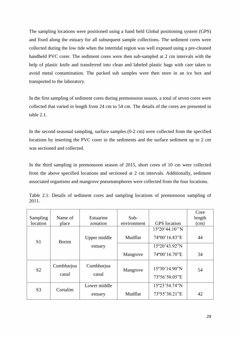
29
The sampling locations were positioned using a hand held Global positioning system (GPS)
and fixed along the estuary for all subsequent sample collections. The sediment cores were
collected during the low tide when the intertidal region was well exposed using a pre-cleaned
handheld PVC corer. The sediment cores were then sub-sampled at 2 cm intervals with the
help of plastic knife and transferred into clean and labeled plastic bags with care taken to
avoid metal contamination. The packed sub samples were then store in an ice box and
transported to the laboratory.
In the first sampling of sediment cores during premonsoon season, a total of seven cores were
collected that varied in length from 24 cm to 54 cm. The details of the cores are presented in
table 2.1.
In the second seasonal sampling, surface samples (0-2 cm) were collected from the specified
locations by inserting the PVC corer in the sediments and the surface sediment up to 2 cm
was sectioned and collected.
In the third sampling in premonsoon season of 2015, short cores of 10 cm were collected
from the above specified locations and sectioned at 2 cm intervals. Additionally, sediment
associated organisms and mangrove pneumatophores were collected from the four locations.
Table 2.1: Details of sediment cores and sampling locations of premonsoon sampling of
2011.
Sampling
location
Name of
place
Estuarine
zonation
Sub-
environment GPS location
Core
length
(cm)
S1 Borim Upper middle
estuary
Mudflat
15º20’44.10’’N
74º00’16.83”E 44
Mangrove
15º20’43.92”N
74º00’16.70”E 34
S2 Cumbharjua
canal
Cumbharjua
canal Mangrove 15º30’14.90”N
73º56’50.05”E
54
S3 Cortalim Lower middle
estuary Mudflat
15º23’54.74”N
73º55’30.21”E 42

30
Mangrove
15º23’54.99”N
73º55’30.86”E 40
S4 Chicalim Lower estuary Mudflat
15º24’01.07”N
73º50’47.36”E 30
Mangrove
15º23’56.94”N
73º50’47.88”E 24
2.3 Laboratory analysis
2.3.1 pH
The pH of each sub sample was measured using a Themo Orion 420A+ pH/mV/ temperature
meter with temperature compensation. The pH meter was calibrated using a three point
calibration using freshly prepared buffer solutions of 4.01, 7.00 and 10.1. The pH was
measured by inserting the electrode into the sediment subsamples and the pH was noted from
the digital meter display.
2.3.2 Sediment components (sand, silt and clay) analysis
The percentage of sand, silt and clay in the sediment subsamples was determined by the
procedure proposed by Folk (1974). Sand, silt, and clay fractions contain particles whose
diameters range from 2000 to 62.5 µm, 62.5 to 3.91 µm, and less than 3.91 µm, respectively.
About 15 g of each dried subsample were placed in a beaker with 1000 ml of distilled water.
The samples were lightly disaggregated with a glass stirring rod. The sediments were then
allowed to settle and after 24 hours the overlying water was decanted. This step was repeated
at least 4 to 5 times to remove salinity that was tested using a solution of AgNO3.
10 ml of 10 % sodium hexametaphosphate (calgon) was added to dissociate the clay particles
because of the unbalanced electrostatic charges on most clay particles that will cause the clay
particles to aggregate or flocculate in suspensions, unless a dispersant is added to inhibit
flocculation. After 24 hours, 5 ml of 30 % Hydrogen peroxide was added to oxidize the
organic matter. The sediment was wet sieved on a 63 µ screen to separate the sand and mud
(silt and clay) fractions. The sand fraction was collected in a pre-weighed 100 ml beaker and
dried in an oven at 60 ºC. Grain size of the mud fraction was determined in a constant

31
temperature room by pipette technique which is based on settling velocities of particles
calculated from Stokes' Law wherein a particle falling freely through a quiescent fluid will
cease to accelerate when the frictional force exerted on the particle by the fluid exactly
balances the downward force of gravity on the particle. The velocity of the particle under
these conditions is called the settling velocity. The solution with mud in the cylinder was
homogenized using a stirrer and stirring time was noted. A pipette withdrawal of 25 ml was
taken at time corresponding to time intervals (Table 2.2) of 8Φ by inserting the pipette up to
10cm depth from the solution level in the cylinder. The pipetted solution was then transferred
into a pre-weighed 100 ml beaker and dried in an oven at 60 ºC. The oven dried beakers
containing sand and silt were then weighed and the percentage of sand, silt and clay was
determined and calculated as follows
Sand (%) = (Weight of sand/ Total weight of sediment) * 100
Clay (%) = [((Weight of clay* 1000 / 25) - 1) / Total weight of sediment)] * 100
Silt (%) = 100 – (Sand % + Clay %)
Table 2.2: Time schedule used for pipette analysis
Size Depth to which pipette
was inserted Time after which suspension was pipetted out
Φ (cm) (Hours: Minutes: Seconds)
28 ºC 29 ºC 30 ºC 31 ºC 32 ºC
4 20 00:00:48 00:00:46 00:00:46 00:00:44 00:00:44
5 10 00:01:36 00:01:34 00:01:32 00:01:29 00:01:28
6 10 00:06:25 00:06:15 00:06:06 00:06:57 00:05:52
7 10 00:25:40 00:25:02 00:24:25 00:24:49 00:23:27
8 10 01:42:45 01:40:13 01:37:42 01:37:15 01:33:51
9 10 06:30:00 06:40:40 06:32:50 06:32:10 06:11:30
10 10 27:06:00 26:30:00 -- -- --

32
2.3.3 Clay minerals analysis
The method of Rao and Rao (1995) was adopted for the analysis of clay minerals. The
procedure for separation of clay sediment fraction is the same as that for pipette analysis. The
clay suspension was pipetted out at 10 cm depth to a 100 ml beaker at 9 Φ from the 1000 ml
cylinder containing the mud suspension. 5 ml of glacial acetic acid and 10 ml hydrogen
peroxide was added to render the clay free of carbonates and organic matter and stirred well.
The contents of the beaker were allowed to settle for 24 hours. The clear solution above the
settled clay was decanted and distilled water was added. Addition of distilled water followed
by decantation was repeated several times to free the clay from excess reagents. Slides for
analysis of clay minerals were prepared by pipetting 1 ml of the concentrated clay suspension
onto a pre-numbered glass slide and uniformly spreading it across the slide. Extreme care was
taken to obtain uniform distribution of clay and to avoid size sorting. The slides were further
air dried and preserved in a box away from moisture till further analysis. For analysis by X-
ray diffractometer, the slides were processed by exposing them to ethylene glycol vapors at
100 ºC for 1 hour in a glass desiccator. The slides were then scanned on a Rigaku X-ray
diffractometer (Ultima IV) apparatus using nickel- filtered CuKα as target and scanning
between 3 º to 30 º 2Ɵ at 1.2º 2Ɵ / min. Clay minerals were then identified and quantified
following the semi-quantitative method of Biscaye (1965). The clay mineral analyses were
carried out in the sedimentology laboratory of the National Institute of Oceanography (NIO),
Goa.
2.3.4 Magnetic susceptibility measurements
For the measuring of magnetic susceptibility, a known weight of sediment sample was
packed in a 10 cc plastic sample container, which was wrapped with a plastic film to reduce
the possibility of cross contamination and generally to keep the sediment immobile within the
sample container while handling the sample. The containers with the packing material are
pre-measured for mass and susceptibility and the values were corrected.
A Bartington MS2 system was used for magnetic susceptibility measurements. The high (4.7
kHz) and low (0.47 kHz) frequency measurements were determined using a dual frequency
Bartington MS2 susceptibility meter. Magnetic susceptibility (χ) measurements of very weak
samples were carried out employing the more sensitive Agico’s Kappabridge KLY-4S

33
instrument. Frequency dependent susceptibility (χfd%) was calculated using the formula (χlf-
χhf)/ χhf *100 where χlf is magnetic susceptibility at low frequency and χhf is susceptibility at
high frequency.
Anhysteretic remanence magnetization (ARM) was imparted in a steady 0.05 Mt field
superimposed over decreasing alternating field from 100 mT to 0 mT using a Molspin A.F.
demagnetizer. ARM created within the sample was then measured using a Molspin spinner
magnetometer.
Isothermal remnant magnetization (IRM) was acquired by first exposing the samples to series
of successively larger fields along one direction and then in the opposite direction (backfields
-20mT, -30mT, -40mT, -100mT, -200mT and -300mT) using a Pulse magnetizer (Magnetic
measurement Ltd.). After each forward and reverse field (DC magnetization), samples were
measured using the Molspin spinner magnetometer. The IRM at 3T is referred as the
saturation isothermal remnant magnetization (SIRM).
Using the above parameters various other parameters were calculated in terms of magnetic
concentration, mineralogy and grain size as summarized by Thomson and Oldfied (1986) and
Oldfield (1999). The descriptions of different parameters are presented in table 2.3.
Table 2.3: Magnetic susceptibility parameters, their definitions and implications
Magnetic parameters Definitions/ formulas Implications
1.Magnetic
susceptibility χ (10-8
m3/ kg)
It indicates the degree of
magnetization of a material in
response to an applied magnetic
field.
χ = M/H
Where M is the magnetization of the
material and
H is the magnetic field strength.
Proportional to the
concentration of magnetic
minerals.
2. Frequency Variation in χ between low (0.47 Used to detect the presence of
ultrafine (<0.03 μm)

34
dependent
susceptibility, χfd (%)
kHz) and high (4.7 kHz) frequency.
Defined as (χlf -χhf/χlf) x 100 where χlf
is the susceptibility at low frequency
and χhf is the susceptibility at high
frequency.
superparamagnetic ferrimagnetic
minerals occurring as crystals
produced largely by biochemical
processes
3.Isothermal
remanent
magnetization, IRM
(10-5 Am2/kg-1)
Magnetization acquired
instantaneously in an external field
Proportional to the
concentration of magnetic
minerals.
4.Anhysteretic
remanent
magnetization, ARM
(10-5
Am2/kg)
Magnetization acquired by the
combined effects of a large
alternating field and a small DC
field
ARM gives an estimation of
the concentration and presence
of fine grain minerals.
5. Susceptibility of
ARM, χARM (10-
8m
3/kg-1)
It is a form of normalized ARM for
the strength of a steady field
Proportional to the
concentration of magnetic
minerals of stable single
domain size range
6. Saturation
isothermal remanent
magnetization ,
SIRM (10-5
Am2/kg)
It is measured as the highest volume
of magnetic remanence that can be
produced in a sample by applying a
very high field
It is a characteristic of mineral
type and concentration.
7. S-ratio (%) It is defined as IRM (-300
mT)/SIRM.
S-ratio provides a measure of
the relative proportions of
ferrimagnetic and
antiferromagnetic minerals
(high ratio = relatively
high proportion of magnetite)
8. χ ARM/χ It is the ratio of the susceptibility of
Anhysteretic remnant magnetization
to magnetic susceptibility.
Indicative of magnetic grain
size of ferrimagnetic minerals
High values indicate
significant stable single
domain (magnetite) grains.
9. χ ARM/ SIRM It is the ratio of the susceptibility of Indicative of magnetic grain

35
(10-3
A-1
m) Anhysteretic remnant magnetization
to Saturation isothermal remnant
magnetization.
size
2.3.5 Total organic carbon estimation
An estimate of total organic carbon (TOC) was used to assess the amount of organic matter in
sediments. The total organic carbon percentage in sediments was determined following the
chromic acid wet oxidation method protocol of Walkley and Black (1934). The method is
based on the principle wherein oxidisable matter in the sediment is oxidised by 1 N K2Cr2O7
solution. The reaction is assisted by the heat generated when two volumes of H2SO4 are
mixed with one volume of the dichromate. The remaining dichromate is titrated with ferrous
ammonium sulfate. The titre is inversely related to the amount of Carbon present in the
sediment sample.
Prior to analysis, all glassware was rinsed with chromic acid and distilled water, followed by
drying in an oven. 0.5 g of sediment was weighed on a digital 4 decimal weighing balance
and transferred to a 500 ml conical flask. 10 ml of 1 N K2Cr2O7 solution was added to the
flask using a graduated burette followed by 20 ml of concentrated H2SO4 with silver sulfate
(AgSO4) to prevent oxidation of chloride ions. The flask was gently swirled for 1 minute to
mix the contents and allowed to react for 30 minutes. After 30 minutes, 200 ml of distilled
water was added to the flask, followed by 10 ml of 85 % phosphoric acid (H3PO4) and 0.2 g
of Sodium Fluoride (NaF). The solution was then back-titrated with 0.5 N Ferrous
ammonium sulfate solution using diphenylamine as an indicator to a one-dropt end point
(brilliant green). Standardization blank was run following the same procedure.
The percentage of organic carbon was calculated as follows:
TOC % = 10 (1-T/S) * F
Where S= Volume in ml of Ferrous ammonium sulfate used in blank titration
T= Volume in ml of Potassium dichromate used in sample titration
F=Factor which is derived as
36
F= (1.0N)*12/4000 * 100/ Sample weight
=0.6
where sample weight is 0.5 g and 12/4000 is the milli equivalent weight of Carbon.
2.3.6 Analysis of bulk sediment chemistry
For analysis of total/bulk metal concentrations in sediments, sediment samples were digested
by the total decomposition procedure using strong acids HF, HClO4 and HNO3 given by
Jarvis and Jarvis (1985). 0.2 g of oven dried sediments were homogenized and weighed on an
electronic weighing balance and transferred to pre-cleaned Teflon beakers. To this, 10 ml of
acid mixture i.e. HF: HNO3:HClO4 in the ratio 7:3:1 was slowly added to avoid excessive
frothing and was completely dried on an electric hot plate at 150 ºC. After drying, 5 ml of the
acid mixture was added and dried on the hot plate for 1 hour. 2 ml of concentrated HNO3 was
then added followed by complete drying. After ensuing complete drying and the resultant
residue was dissolved in10 ml of 1:1 HNO3 and the clear solution was transferred into an acid
washed 50 ml volumetric flask and diluted up to the mark with millique water. The digested
sediment extracts were then analyzed using an Atomic Absorption spectrophotometer (Flame
AAS). Sediment standard reference 2702 obtained from National Institute of Standards and
Technology (NIST) was digested following the same procedure.
2.3.7 Clay fraction chemistry analysis
The clay fraction of sediments was separated using the pipette technique at 9 Φ as described
in section 2.3.2. The clay fraction was collected in a 500 ml beaker after pipetting the clay
suspension from the cylinder containing the mud suspension by inserting the pipette at 10 cm
depth. The collected clay suspension was allowed to settle for 24 hours followed by oven
drying at 60 ºC. The dried clay was then collected and stored in plastic vials. 0.2 g of the
dried clay was then digested following the procedure for digestion of bulk sediments as
described in section 2.3.6 and metals were analyzed using an flame AAS.
2.3.8 Speciation of metals
An analytical procedure developed by Tessier et al. (1979) involving sequential chemical
extractions of sediments for the partitioning of trace metals into five fractions: exchangeable,
bound to carbonates, bound to Fe-Mn oxides, bound to organic matter/ sulfides, and residual
was employed. The speciation of metals in sediments furnishes detailed information about the
origin, mode of occurrence, biological and physicochemical availability, mobilization, and

37
transport of trace metals. The following steps were followed for extraction of each of the five
phases/ fractions.
(i) Exchangeable fraction (F1): Exchangeable metals are a measure of those traces metals
which are released most readily to the environment. This fraction involves weakly adsorbed
metals retained on the solid surface by relatively weak electrostatic interaction, metals that
can be released by ion-exchangeable processes. Exchangeable fraction can be released by the
action of cations such as K, Ca, Mg or NH4 displacing metals weakly bond electrostatistically
organic or inorganic sites. The common reagents used for the extraction of metals in this
fraction are MgCl2 or sodium acetate.
1 g of dried ground sediment was weighed and transferred into plastic capped tubes. 8 ml of
magnesium chloride solution (1 M MgCl2, pH 7.0) was added and the sediment was extracted
at room temperature for 1 h with continuous agitation. The sediment suspension was
centrifuged at 8000 rpm for 10 minutes and the supernatant was collected for analysis of
metals. The residue was washed with millique water and decanted.
(ii) Bound to Carbonates (F2): The carbonate fraction is a loosely bound phase and bound
to changes with environmental factors such as pH. This fraction is sensitive to pH changes,
and metal release is achieved through dissolution of a fraction of the solid
material at pH close to 5.0. The most popular reagent used for the extraction of trace metals
from carbonates phases in sediments is 1 M sodium acetate adjusted to pH 5.0 with acetic
acid.
Metals in the residue from step (i) were leached at room temperature with 8 mL of 1M
Sodium acetate (NaOAc) adjusted to pH 5.0 with acetic acid (HOAc). Continuous agitation
was maintained and the time necessary for complete extraction was evaluated. The
suspension was centrifuged at 8000 rpm for 10 minutes and the supernatant was collected for
analysis of metals. The residue was then washed with millique water and decanted.
(iii) Bound to Fe-Mn Oxides (F3): This phase is referred to as sink for heavy metals. The
scavenging of metals by the oxides, present as coating on mineral surfaces or as fine discrete
particle can occur as a combination of the precipitation, adsorption, surface complex

38
formation and ion exchange. Hydroxylamine, oxalic acid and dithionite are the most
commonly used reagents to extract metals associated with this phase.
The residue from step (ii) was extracted with 20 mL of 0.04 M Hydroxylamine hydrochloride
(NH20H-HCl) in 25% (v/v) acetic acid (HOAc) at 96 ± 3 ºC with occasional agitation for 5
hours. The suspension was centrifuged at 8000 rpm for 10 minutes and the supernatant was
collected for analysis of metals. The residue was then washed with millique water and
decanted.
(iv) Bound to Organic Matter/ Sulfides (F4): In organic phase, metals bound to this phase
are assumed to stay in the sediment for longer periods but may be immobilized by
decomposition process. Under oxidizing conditions, degradation of organic matter can lead to
a release of soluble trace metals bound to this component. The extracts obtained during this
step also contain metals bound to sulfides. The most commonly used reagent for the
extraction of metals in organic phases is hydrogen peroxide with ammonium acetate re-
adsorption or precipitation of released metals
To the residue from step (iii), 3 mL of 0.02 M HN03 and 5 mL of 30% H2O2 adjusted to pH 2
with HN03 were added and the mixture was heated to 85 ± 2 ºC for 2 h with occasional
agitation. A second 3 ml aliquot of 30 % H2O2 (pH 2 with HNO3) was then added and the
sample was heated again to 65 ± 2 ºC for 3 h with intermittent agitation. After cooling, 5 mL
of 3.2 M ammonium acetate NH4OAc in 20 % (v/v) HN03 was added and the sample was
diluted to 20 ml and agitated continuously for 30 min. The addition of ammonium acetate
(NH4OAc) is designed to prevent adsorption of extracted metals onto the oxidized sediment.
The suspension was centrifuged at 8000 rpm for 10 minutes and the supernatant was
collected for analysis of metals. The residue was then washed with millique water and
decanted.
(v) Residual (F5): Metals in the residual fraction are associated with the silicate matrix and
are resistant metals bound to primary and secondary minerals in the crystalline lattice. Its
destruction is achieved by digestion with strong acids, such as HF, HClO4, HCl and HNO3.
The residue from step (iv) was then transferred into a teflon beaker and oven dried at 60 ºC.
The residue was further digested using a HF-HNO3-HClO4 mixture following the procedure
for total/ bulk metal analysis.

39
The extracts from the five steps described above were then aspirated into an AAS for analysis
of metals. The first four fractions are known as the bioavailable fractions and the first two
fractions are knows as the labile fractions.
2.4 Sampling of biota
Sediment associated organisms and mangrove pneumatophores were collected from the
specified sampling locations during the premonsoon season in 2015. From each sampling
location, Gastropod organisms which were easily available on the surface and subsurface
were handpicked from the sediments and transferred into clean polythene bags and stored in
an ice box. The organisms were washed with distilled water to remove dirt and sediments
particles that adhered to the organisms. The organisms were then identified and refrigerated
at - 23 ºC in plastic zip log bags until further analysis.
Mature pneumatophores were randomly collected surrounding the sediment core. Mangrove
pneumatophores of Avicennia officinalis were collected at locations S1, S2 and S3, whereas
pneumatophores of Sonneritia alba was collected at S4. Pneumatophores were cut at the
sediment surface with a stainless steel knife at each sediment core site. Three strands of
pneumatophores were pooled together to make one sample for each core site. Pneumatophore
samples were stored in a zip-lock plastic bag and transferred to an ice box and transported to
the laboratory for preservation at 4 °C until further processing. The schematic diagram for
processing of biota samples to study bioaccumulation of metals is presented in figure 2.3.
2.4.1 Metals in sediment associated organism’s tissues
The frozen samples were brought to room temperature. Gastropod shells were opened by
breaking their shells. A pair of stainless steel forceps was used to dislodge and to remove the
soft tissues from the shell. The tissue of each sub sample was oven dried in a glass petri dish
to a constant weight at 60 ºC for 72 hours (Ferreira et al., 2004). The dried samples were
pulverized together into fine powder using a porcelain mortar and pestle. The digestion of the
tissue was carried out by taking 0.5 g of tissue sample in a Teflon beaker with 2 ml of HNO3
and 1 ml of HClO4 at 120 ºC for 3 hours. The digest was diluted with millique water and the
final volume was made up to 25 ml in a glass volumetric flask and stored in pre-cleaned

40
plastic bottles (Yüzereroglu et al., 2010). Metals in the extracts were then analyzed using the
AAS.
Figure 2.3: Schematic flowchart of steps followed in processing of biota samples for metal
analysis by Atomic absorption spectrophotometer.
2.4.2 Metals in mangrove pneumatophores
The collected pneumatophores were washed with distilled water to remove dirt and sediment
particles, and dried in an oven at 60 °C for 24 h. Oven-dried samples were ground to fine
powder using a porcelain mortar and pestle and kept in a plastic container for chemical
analysis (Nath et al., 2014). The digestion of dried pneumatophore samples was carried out
by adding HNO3 and H2O2 in teflon beakers at 90 ºC for 2 hours. The digested extracts were
then diluted to 25 ml with millique water and were analyzed using AAS (MacFarlane and
Burchette, 2002).

41
2.5 Atomic Absorption Spectrophotometry
The digested bulk sediment, clay fraction, sediment fractions, gastropod tissue and
pneumatophore extracts were analyzed for metals using a Varian AA240FS flame atomic
absorption spectrometry (AAS) with an air/acetylene flame for all metals at specific
wavelengths. The bulk sediment and clay extracts were analyzed for Al, Fe, Mn , Cr, Co, Ni,
Cu and Zn whereas sediment fractions were analyzed for metals, Fe, Mn, Cr, Co, Cu and Zn.
Biota samples i.e. organism tissue and pneumatophore fraction were analyzed for metals Fe,
Mn, Cr, Co, Ni, Cu and Zn. The accuracy of the analytical method was obtained by the
standard reference 2702 from National Institute of Standards and Technology (NIST). The
average recoveries and ± standard deviations found for metals Fe, Mn, Cr, Co, Ni, Cu and Zn,
were 89±12, 91±15, ±14, 74±12, 86±16, 82±15, and 84±16 respectively. Precision was
monitored by running triplicates after every ten samples and the relative standard deviation
was generally <6 % for major and trace elements. Analytical grade reagents and standards
were used in all the analysis
2.6 Data processing
2.6.1. Ternary diagram, Isocon diagram and statistical analysis
To understand the hydrodynamic conditions in which sediments have been deposited, the
data of the cores were plotted on a ternary diagram by Pejrup (1988). According to his
classification, lines of constant clay content of the mud fraction (smaller than 4 phi) are
drawn to divide the triangle. The finest part of the mud fraction (smaller than 4 phi) of
estuarine sediments very often has a constant textural composition, because these small grain
sizes occur in the water as part of sediment flocs. The percentage of this flocculated grain
size population in the mud fraction of estuarine sediment can therefore be used as a simple
indicator of the hydrodynamic conditions under which deposition took place. Sections
labelled I to IV, (Figure 2.4) which indicate increasingly high energy hydrodynamic
conditions. The sediments are classified according to their sand content into four sections, A
to D. The triangle is thus divided into 16 sections, each of which can be named by a letter
indicating the type of sediment and a number indicating the hydrodynamic conditions during
deposition (Shi, 1992). Section I represents calm conditions, II – relatively calm conditions,
III- relatively violent conditions and IV- violent conditions. In this scheme, class A-IV
designates the highest, class D-I the lowest energy regime.
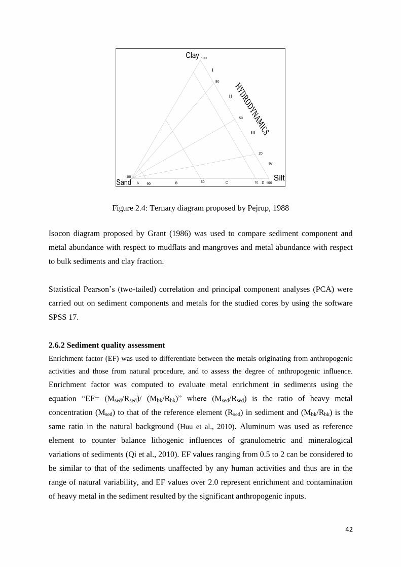
42
Figure 2.4: Ternary diagram proposed by Pejrup, 1988
Isocon diagram proposed by Grant (1986) was used to compare sediment component and
metal abundance with respect to mudflats and mangroves and metal abundance with respect
to bulk sediments and clay fraction.
Statistical Pearson’s (two-tailed) correlation and principal component analyses (PCA) were
carried out on sediment components and metals for the studied cores by using the software
SPSS 17.
2.6.2 Sediment quality assessment
Enrichment factor (EF) was used to differentiate between the metals originating from anthropogenic
activities and those from natural procedure, and to assess the degree of anthropogenic influence.
Enrichment factor was computed to evaluate metal enrichment in sediments using the
equation “EF= (Msed/Rsed)/ (Mbk/Rbk)” where (Msed/Rsed) is the ratio of heavy metal
concentration (Msed) to that of the reference element (Rsed) in sediment and (Mbk/Rbk) is the
same ratio in the natural background (Huu et al., 2010). Aluminum was used as reference
element to counter balance lithogenic influences of granulometric and mineralogical
variations of sediments (Qi et al., 2010). EF values ranging from 0.5 to 2 can be considered to
be similar to that of the sediments unaffected by any human activities and thus are in the
range of natural variability, and EF values over 2.0 represent enrichment and contamination
of heavy metal in the sediment resulted by the significant anthropogenic inputs.

43
Geo-accumulation index- Igeo (Muller, 1979) was computed to assess the level of metal
contamination in sediments using the equation “Igeo= Log2 (Cn/1.5Bn)” where Cn is the
concentration of the metal in the sample and Bn is the background metal concentration in
average shale (Turekian and Wedepohl, 1961). Igeo values are categorized based on level of
pollution into seven classes viz. “Very strongly polluted”-Igeo class 6 (Igeo >5); “Strong to
very strong”-Igeo class 5 (Igeo 4–5); “Strongly polluted”-Igeo class 4 (Igeo 3–4);
“Moderately to strongly polluted”-Igeo class 3 (Igeo 2–3); “Moderately polluted”-Igeo class
2 (Igeo 1–2); “Unpolluted to moderately polluted—Igeo class 1 (Igeo 0–1) and “Unpolluted”-
Igeo class 0 (Igeo < 0).
Concentration of metals in the bioavailable fractions (sum of first four fractions) and bulk
sediments was compared with the sediment quality values (SQV) following screening quick
reference table (SQUIRT) (Table 2.4) developed by NOAA (Buchman, 1999) and labile
fractions (exchangeable and carbonate) was compared with the Risk Assessment Code- RAC
(Perin et al., 1985) to explain the toxicity level of the metals (Table 2.5).
Table 2.4 Screening Quick Reference table for metals in marine sediments (Buchman, 1999)
Metal Threshold
Effect level
(TEL)
Effects
range level
(ERL)
Probable
Effects level
(PEL)
Effects
Range
Median
(ERM)
Apparent Effects Threshold (AET)
Fe NA NA NA NA 22 % / 22000 ppm (Neanthes)
Mn NA NA NA NA 260 (Neanthes)
Cr 52.30 81.00 160.00 370.00 62 (Neanthes)
Co NA NA NA NA 10 (Neanthes)
Ni 15.90 20.90 42.80 51.60 110 (Echinoderm larvae)
Cu 18.70 34.00 108.00 270.00 390 (Microtox and Oyster Larve)
Zn 124.00 150.00 271.00 410.00 410 (Infaunal community)
*All values are in ppm or indicated otherwise

44
Sediment guidelines
Threshold Effect level (TEL) Maximum concentrations at which no toxic
effects are observed
Effects range level(ERL)
10th
percentile values in effects or toxicity
may begin to be observed in sensitive
species.
Probable Effects level(PEL) Lower limit of concentrations at which toxic
effects are observed
Effects Range Median(ERM) 50th
percentile value in effects
Apparent Effects Threshold (AET) Concentrations above which adverse
biological impacts are observed.
Table 2.5: Classification of risk assessment code (RAC) by Perin et al. (1985)-.
RAC Criteria (%)
No risk < 1
Low risk 1-10
Medium risk 11-30
High risk 31-50
Very high risk > 50
2.6.3 Bioaccumulation tools to estimate uptake of metals by biota.
Biosediment accumulation factor (BSAF) was used to investigate the capability of the sediment
associated organisms to accumulate heavy metal from the environment and hereby, suggesting its
possibility as biomonitor for heavy metals. BSAF was calculated to assess the bioaccumulation
of metals by organisms. BSAF was calculated using the equation
“BSAF = Cx/ Cs”
where Cx and Cs are metal concentrations in biota and sediments, respectively (Szefer et al.,
1999). If the BSAF >1, bioaccumulation is considered to reach threshold with respect to
contamination. Based on the values calculated, the gastropod could be classified into a few

45
groups such as macro concentrator (BSAF >2), micro concentrator (1< BSAF <2) or de-
concentrator (BSAF <1) as proposed by Dallinger (1993).
Bioconcentration Factor (BCF) was computed on similar lines to BSAF, to assess metal
accumulation in pneumatophores relative to environmental loadings using the equation
“BCF= metal concentration in pneumatophore/ Metal concentration in sediments”
(MacFarlane et al., 2007).

46
Chapter 3
Results
and
Discussions

47
Section 3.1: Sediment cores collected in premonsoon of 2011.
3.1A Mangroves
3.1. A.1 Sediment components (pH, sand, silt, clay and total organic carbon)
The range and average values of sediment pH, grain size, and total organic carbon within the
mangroves of the Zuari estuary are presented in table 3.1.1 (a). The sediment core collected
from the upper middle region (S1) of the Zuari estuary (Borim) during premonsoon season in
2011 was with length 34 cm. The sediments were of near neutral pH and clay was the
dominant sediment size fraction followed by silt and sand. The pH in this core ranged from
6.12 to 7.54 (average 7.09). The sand content ranged from 0.49 % to 6.14 % (average 2.28
%), whereas silt ranged from 22.52 % to 48.41 % (average 36.8 %) and clay ranged from
48.00 % to 71.68 % (average 60.92 %). Total organic carbon (TOC) ranged from 2.50 % to
3.53 % (average 2.85 %) in the mangrove sediments of S1. In sediment core of length 54 cm
collected from the mangrove sub-environment of the Cumbharjua canal (S2) during the
premonsoon season, the pH was weakly acidic ranging from 5.9 to 6.5 (average 6.19). The
sand content ranged from 2.28 % to 13.85 % (average 5.82 %). Silt was the dominant
sediment component in this core and ranged from 24.51 % to 69.39 % (average 48.55 %).
The clay percentage in the core ranged between 26.90 % and 61.64 % (average 45.64 %) and
the TOC varied from 1.64 % to 2.96 % (average 2.13 %). In sediment core collected from the
Cortalim representing the lower middle estuarine mangroves (S3) was with 40 cm in length
and the sediment pH was of near neutral nature, ranging from 6.44 to 6.94 (average 6.65).
Clay was the dominant fraction in the sediments followed by silt and sand. Sand percentage
ranged from 0.46 % to 2.17 % (average 1.04 %). Silt percentage ranged between 29.38 % and
55.13 % (average 37.01 %) whereas clay ranged from 43.52 % to 68.88 % (average 61.95 %).
TOC in core S3 ranged between 1.31 % and 3.18 % (average value of 2.52 %). The sediment
core collected from Chicalim mangrove region represented the lower estuary (S4) was of 24
cm length. The pH of the sediments was near neutral, ranging from 6.73 to 7.01 (average
6.86). The dominant sediment fraction in this core was sand that ranged between 29.98 % and
84.74 % (average 57.5 %). Silt content in the core sediments ranged between 3.21 and 44.05
% (average 19.88 %). Clay percentage however, was higher than silt, but less than sand and
ranged between 7.68 % and 34.88 % (average of 22.61 %) and the TOC content ranged
between 0.37 % and 1.99 % (average of 1.26 %).
48
The distribution of sediment components with depth in cores S1, S2, S3 and S4 are presented
in figure 3.1.1. The sediment components in core S1 exhibited distinct distribution patterns.
The pH was relatively constant with depth except at 8 cm where the profile showed a
decreased peak. Sand distribution in core S1 showed percentages above average up to 26 cm
from bottom, followed by constant percentages below the average towards the surface. Silt
and clay distribution patterns compensated each other with fluctuations. The distribution of
TOC with depth in core S1 was constant up to 20 cm and showed an increased peak at 14 cm
that corresponded to the higher clay values followed by lower than average TOC values up to
the surface. In core S2, the pH exhibited a constant distribution pattern with depth. The sand
percentage decreased from the core base to 22 cm followed by an increase towards the
surface. The clay values decreased towards the surface and was compensated by an increase
in silt with fluctuating trends. The TOC percentage was constant up to 26 cm followed by an
increased peak at 24 cm. The distribution of pH in core S3 was relatively constant with depth
with minor peaks at 26 cm, 20 cm and 12 cm. The distribution of sand, silt and clay
percentages showed little variation with depth. The sand percentage showed a uniform
distribution pattern towards the surface from the base of the core. The distribution of silt was
constant towards the surface with the exception of higher silt percentages at 40 cm, 32 cm, 16
cm and 8cm. The clay distributions compensated silt. TOC in core S3 showed higher than
average but constant values from the base of the core up to 24 cm. Further above, values
showed large fluctuations with an overall decreasing trend. In core S4, the pH showed a
uniform distribution with depth. The sand content decreased towards the surface and that was
compensated by an increase in silt percentage. The clay percentage gradually increased
towards the surface along with silt. In core S4 collected from the lower estuarine region, large
amount of calcareous material was noted in the deeper portion. The higher sand percentage in
the lower part may have been the result of the presence of coarse calcareous sand, gastropods
shells, and bivalves (Welle et al., 2004). The TOC percentage increased towards the surface
along with the finer sediments.
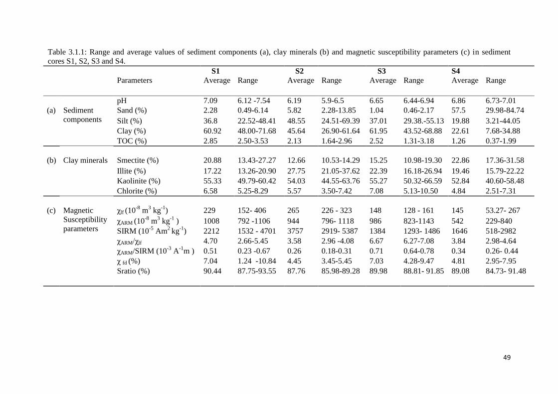
49
Table 3.1.1: Range and average values of sediment components (a), clay minerals (b) and magnetic susceptibility parameters (c) in sediment
cores S1, S2, S3 and S4.
S1 S2 S3 S4 Parameters Average Range Average Range Average Range Average Range
pH 7.09 6.12 -7.54 6.19 5.9-6.5 6.65 6.44-6.94 6.86 6.73-7.01
(a) Sediment
components
Sand (%) 2.28 0.49-6.14 5.82 2.28-13.85 1.04 0.46-2.17 57.5 29.98-84.74
Silt (%) 36.8 22.52-48.41 48.55 24.51-69.39 37.01 29.38.-55.13 19.88 3.21-44.05
Clay (%) 60.92 48.00-71.68 45.64 26.90-61.64 61.95 43.52-68.88 22.61 7.68-34.88
TOC (%) 2.85 2.50-3.53 2.13 1.64-2.96 2.52 1.31-3.18 1.26 0.37-1.99
(b) Clay minerals Smectite (%) 20.88 13.43-27.27 12.66 10.53-14.29 15.25 10.98-19.30 22.86 17.36-31.58
Illite (%) 17.22 13.26-20.90 27.75 21.05-37.62 22.39 16.18-26.94 19.46 15.79-22.22
Kaolinite (%) 55.33 49.79-60.42 54.03 44.55-63.76 55.27 50.32-66.59 52.84 40.60-58.48
Chlorite (%) 6.58 5.25-8.29 5.57 3.50-7.42 7.08 5.13-10.50 4.84 2.51-7.31
(c) Magnetic
Susceptibility
parameters
χlf (10-8
m3 kg
-1) 229 152- 406 265 226 - 323 148 128 - 161 145 53.27- 267
χARM (10-8
m3 kg
-1 ) 1008 792 -1106 944 796- 1118 986 823-1143 542 229-840
SIRM (10-5
Am2
kg-1
) 2212 1532 - 4701 3757 2919- 5387 1384 1293- 1486 1646 518-2982
χARM/χlf 4.70 2.66-5.45 3.58 2.96 -4.08 6.67 6.27-7.08 3.84 2.98-4.64
χARM/SIRM (10-3
A-1
m ) 0.51 0.23 -0.67 0.26 0.18-0.31 0.71 0.64-0.78 0.34 0.26- 0.44
χ fd (%) 7.04 1.24 -10.84 4.45 3.45-5.45 7.03 4.28-9.47 4.81 2.95-7.95
Sratio (%) 90.44 87.75-93.55 87.76 85.98-89.28 89.98 88.81- 91.85 89.08 84.73- 91.48

50
Figure 3.1.1: Distribution of sediment components with depth in mangrove cores S1, S2, S3
and S4.
The sediments exhibited wide variations in grain size at different sampling stations of the
Zuari estuary. The percentage of the coarser sediment decreased towards the upper middle
estuary with a corresponding increase in finer sediment. The high sand content in the lower
estuary sediments was due to the higher hydrodynamic conditions prevailing owing to high
energy waves that prevented the accumulation of finer sediments. High silt content was
observed in the canal sediments whereas clay was notably higher in the lower middle
estuarine sediments. Overall, clay and silt dominated the sediments collected from the upper
middle, lower middle estuary and Cumbharjua canal. Thus, the high-energy conditions in the
lower estuary caused the finer sediments carry in suspension and deposited at places where

51
hydrodynamic conditions were quiet. When the distributions of the sediment components
with depth, amongst the stations, are considered, the lower middle estuary seems to maintain
uniform hydrodynamic conditions with time as shown by constant distribution trends of
sediment components. The higher sand in the lower part of the cores collected from the upper
middle estuary, Cumbharjua canal and the lower estuary indicated that higher energy
hydrodynamic conditions prevailed in the past compared to recent years.
The accumulation of organic matter in estuarine mangrove sediments is controlled by several
factors that include organic matter sources, sedimentation rate, preservation potential and the
decomposition rate of organic materials (Yang et al., 2011). The high TOC percentage in the
core collected from the upper middle estuary that coincided with high clay was attributed to
the enhanced adsorption of organic carbon onto the clay minerals in the low salinity regimes
(Akhil et al., 2013). The increased TOC percentage along with silt in the upper sections of the
core in the Cumbharjua canal may be due to the rapid burial of organic matter. Rapid
sedimentation and burial can enhance TOC preservation that is accomplished by a high influx
of inorganic detritus, biogenic inorganic sediment or organic material (Waples, 2013). The
higher TOC in the lower part of the sediment core of the lower middle estuary might have
been caused either by the additional supply of terrestrial organic matter, better preservation
or increased surface water productivity (Wahyudi and Minagawa, 1997).
Further, to understand the hydrodynamic conditions in which sediments were deposited, the
ternary diagram of sand, silt and clay proposed by Pejrup (1988) was employed (Figure
3.1.2). The data of sediment samples of core S1 and S3 fell in section IID indicating the
sediments were deposited under relatively calm conditions. The sediments of mangrove core
S2 fell in sections IID and IIID revealing the sediments were deposited under relatively calm
to relatively violent depositional conditions. The sediments of core S4 however, fell in
sections IIB, IIC and IIIC suggesting varying hydrodynamic environments, with time at this
location.
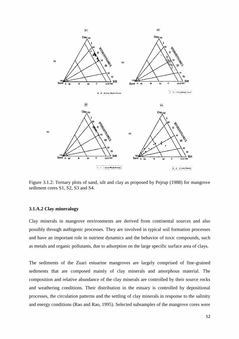
52
Figure 3.1.2: Ternary plots of sand, silt and clay as proposed by Pejrup (1988) for mangrove
sediment cores S1, S2, S3 and S4.
3.1.A.2 Clay mineralogy
Clay minerals in mangrove environments are derived from continental sources and also
possibly through authigenic processes. They are involved in typical soil formation processes
and have an important role in nutrient dynamics and the behavior of toxic compounds, such
as metals and organic pollutants, due to adsorption on the large specific surface area of clays.
The sediments of the Zuari estuarine mangroves are largely comprised of fine-grained
sediments that are composed mainly of clay minerals and amorphous material. The
composition and relative abundance of the clay minerals are controlled by their source rocks
and weathering conditions. Their distribution in the estuary is controlled by depositional
processes, the circulation patterns and the settling of clay minerals in response to the salinity
and energy conditions (Rao and Rao, 1995). Selected subsamples of the mangrove cores were

53
subjected to clay mineral analysis using X-ray Diffraction and the range and average values
obtained are presented in table 3.1.1(b). The clay mineral assemblage of the Zuari estuary
was comprised of kaolinite, smectite, chlorite and illite. Kaolinite was the major clay mineral
at all stations along the estuary followed by illite, smectite and chlorite.
In the mangrove sediment core S1, the percentages of smectite ranged between 13.43 % and
27.27 % (average 20.88%), illite ranged between 13.26 % and 20.90 % (average 17.22 %),
kaolinite ranged between 49.79 % and 60.42 % (average 55.33 %) and chlorite ranged
between 5.25 % and 8.29 % (average 6.58 %). The sediment core S2 collected from the
Cumbharjua canal showed smectite percentages that ranged between 10.53 % and 14.29 %
(average 12.66 %), illite ranged between 21.05 % and 37.62 % (average 27.75 %), kaolinite
ranged between 44.55 % and 63.76 % (average 54.03 %) and chlorite ranged between 3.50
% and 7.42 % (5.57 %). The clay minerals composition of the sediments collected from the
lower middle estuarine mangrove core S3 consisted of smectite that ranged between 10.98 %
and 19.30 % (average 15.25 %), illite ranged between 16.18 % and 26.94 % (average 22.39
%), kaolinite ranged between 50.32 % and 66.59 % (average 55.27 %) and chlorite ranged
between 5.13 % and 10.50 % (average 7.08 %). In the case of the lower estuarine mangrove
sediment core S4, smectite content ranged between 17.36 % and 31.58 % (average 22.86 %),
illite ranged between 15.79 % and 22.22 % (average 19.46 %), kaolinite ranged between
40.60 % and 58.48 % (average 52.84 %) and chlorite ranged between 2.51 % and 7.31 %
(average 4.84 %).
In the distribution of clay minerals with depth (Figure 3.1.3), in the sediment core S1
collected from the upper middle estuary, smectite percentage decreased from the base of the
core up to 14 cm and then increased towards the surface. Illite increased up to 10 cm and then
decreased towards the surface. Kaolinite showed opposite distribution pattern to smectite and
chlorite exhibited opposite distribution pattern to illite. In the clay mineral distributions in
core S2 with depth, smectite displayed little variation, illite showed a fluctuating distribution
pattern with a decrease in percentage from the base of the core up to 22 cm followed by an
increase up to 10 cm and further decreased and then constant values along the average
towards the surface. Kaolinite exhibited an opposite distribution pattern to illite. Smectite and
chlorite percentages decreased up to 18 cm followed by fluctuations around the average line
towards the surface.

54
Figure 3.1.3: Distribution of clay minerals in the mangrove sediment cores S1, S2, S3, and
S4.
In the distribution of clay mineral with depth of the lower middle estuarine mangrove core
S3, smectite exhibited near uniform distribution up to 18 cm followed by fluctuating
distribution towards the surface. The illite showed a minor increase up to 18 cm followed by
a fluctuating distribution towards the surface similar to smectite. Kaolinite values were
constant with depth except for a minor positive peak at 6 cm. Chlorite values decreased up to
30 cm from the base of the core followed by a uniform distribution towards the surface.
Overall, clay minerals showed minor variations in their distributions with depth in this core.
From the distribution of clay minerals with depth in core S4, smectite showed a fluctuating

55
trend with overall decrease towards the surface. Illite showed a minor decrease up to 10 cm
followed by an increase towards the surface. Kaolinite percentage increased up to 18 cm
followed by a steady distribution pattern towards the surface. Chlorite percentages decreased
towards the surface with minor fluctuations.
Clay minerals are good indicators of the source area, weathering intensity and maturity of
modern marine and fluvial sediments. As the distance from the source area increases, the
sediments present a clay mineral assemblage that might have changed in relation to transport,
deposition, remobilization and inputs from tributaries (Guyot et al., 2007). Abundant
kaolinite reflected intense chemical weathering of the rocks along the drainage basin under
humid tropical conditions in the catchment area and marks well developed leached soils and
mature sediments. Feuillet and Fleischer (1980) stated that the estuarine circulation exerts the
dominant influence on the clay mineral distribution. Average clay mineral percentages in the
mangrove sediments indicated that smectite was abundant in core S4, illite in core S2,
kaolinite in core S1 and chlorite in core S3. Smectite being the finest clay and flocculated at
higher salinity explained the higher smectite concentration in the lower estuarine core. A
decrease of kaolinite from the upstream regions towards downstream was noted in Zuari
estuary within the mangrove sediments. The higher values of kaolinite in the upper middle
estuarine sediments have resulted from its characteristic flocculation at low salinity.
Furthermore, the relatively low kaolinite content in the Cumbharjua canal, as compared to the
upper middle and lower middle estuarine sediments, suggested that the Cumbharjua canal
does not make a strong impact with respect to addition of kaolinite but may have supplied a
considerable amount of illite to the Zuari estuary. However, minor amounts of Illite and
chlorite seem to be added as products of weathering of rocks from the catchment area. The
smectite percentage was also high in sediments of the upper middle estuary. Smectite as a
weathering product of the lithological formations in coastal plains and transported into the
Zuari estuary during the monsoon season was reported by Kessarkar et al. (2013). However,
Bukhari and Nayak (1996) have interpreted higher smectite near the mouth as input from sea
side as weathering products of coastal basalts. The input of smectite from the seaside was
possible as continental shelf sediments off Goa contain high smectite (Rao and Rao, 1995).
The clay mineral distributions at each station as a whole did not show much variation with
depth that suggested little change in source in the catchment area. However, smectite and to
some extent illite showed opposite distribution patterns to that of kaolinite. This distribution

56
pattern implied an authigenic transformation process likely taking place, from kaolinite to Fe-
illite/glauconite, through transitory kaolinite - smectite and illite - smectite phases in the
mangrove sediments. The reaction is triggered by high Fe activity in solution generated by
dissolution of Fe oxides and pyrite present in the sediment, at approximately neutral pH and
high salt content in the water (Pugliese-Andrade et al., 2014). Thus, the clay mineral
assemblage reflected the weathering conditions in the catchment area, in addition to the
transportation and depositional processes occurring in the mangrove environments.
3.1.A.3 Magnetic susceptibility
The magnetic parameters that determine the concentration of magnetic minerals are magnetic
susceptibility (χlf), saturation isothermal remnant magnetization (SIRM) and susceptibility of
anhysteretic remnant magnetization (χARM). These parameters increase in denomination as the
concentration of magnetic material in sediment increases. S-ratio was used as a mineral
dependent parameter and values of S-ratio near 100 % indicate a high proportion of
magnetite, whereas lower values indicate an increasing amount of haematite and goethite.
The magnetic grain size is denoted by the frequency dependent susceptibility (χfd) and the
ratios χARM/ χlf and χARM/SIRM. Higher values of these parameters reflect more Stable Single
Domain (SSD) grains and lower values reflect more Multi-Domain (MD) or Super-
Paramagnetic (SP) grains (Dessai et al., 2009; Singh et al., 2013). The range and average
values of magnetic susceptibility parameters in mangrove sediments are presented in table
3.1.1(c).
The magnetic mineral concentration parameters, χlf values of the core S1 collected from the
upper middle estuarine mangroves varied distinctly from 152 ×10-8
m3
kg-1
to 406 ×10-8
m3
kg-1
(average 228.60 ×10⁻⁸
m3
kg-1
), χARM values ranged from 792 ×10-8
m3
kg-1
to 1106 ×10-8
m3
kg-1
(average 1008 ×10-8
m3
kg-1
) and SIRM values ranged from 1532 ×10-5
Am2 kg
-1 to
4701 ×10-5
Am2 kg
-1 (average of 2212×10
-5 Am
2 kg
-1). The inter-parameter ratios of χARM /
χlf, χARM /SIRM vary with magnetic grain size and are used to assess the relative change in
the concentrations of fine magnetic grain sizes (Peters and Dekkers, 2003; Maher, 1988). The
χARM / χlf ratio ranged from 2.66 to 5.45 (average of 4.70) whereas the χARM /SIRM ratio
ranged from 0.23×10⁻³
A-1
m to 0.67×10⁻³
A-1
m (average 0.51×10⁻³
A-1
m). χfd, a parameter
that is a measure of the concentration of ultra-fine magnetic grains in the SP or SSD size

57
range that are produced during pedogenesis, in core S1 ranged from 1.24 % to 10.84 %
(average 7.04 %). The S-ratio % of core S1 ranged from 87.75 % to 93.55 % (average 90.44
%). In the sediment core S2 collected from the Cumbharjua canal, the χlf values ranged from
226 ×10-8
m3
kg-1
to 321 ×10-8
m3
kg-1
(average 264.85×10⁻⁸
m3
kg-1
), χARM values ranged
between 796 ×10-8
m3
kg-1
and 1118×10-8
m3
kg-1
(average 944×10-8
m3
kg-1
) and SIRM
values ranged from 2919×10-5
Am2 kg
-1 to 5387 ×10
-5 Am
2 kg
-1 (average of 3757×10
-5 Am
2
kg-1
). The ratio of χARM / χlf varied between 2.96 and 4.08 (average 3.58) whereas the ratio of
χARM /SIRM in the core ranged between 0.18 ×10⁻³
A-1
m and 0.31 ×10⁻³
A-1
m (average
0.26×10⁻³
A-1
m) and χfd in core S2 ranged from 3.45 % to 5.45 % (average 4.45 %) and the
S-ratio varied between 85.98 % to 89.28 % (average 87.76 %). In the mangrove sediment
core S3 collected from the lower middle estuary magnetic susceptibility parameters, χlf
ranged from 128 ×10-8
m3
kg-1
to 161 ×10-8
m3
kg-1
(average 147×10-8
m3
kg-1
), χARM varied
between 823×10-8
m3
kg-1
and 1143×10-8
m3
kg-1
(average 986×10-8
m3
kg-1
) and SIRM
ranged from 1293×10-5
Am2 kg
-1 to 1486×10
-5 Am
2 kg
-1 (average 1384×10
-5 Am
2 kg
-1). The
values of the ratio of χARM / χlf varied between 6.27 and 7.08 (average of 6.67) and χARM
/SIRM values ranged from 0.64×10⁻³
A-1
m to 0.78×10⁻³
A-1
m (average 0.71×10⁻³
A-1
m). χfd
values ranged from 4.28 % to 9.47 % (average 7.03) and S-ratio varied from 88.81 % to
91.85 % (average 89.98 %). In the lower estuary core S4, the magnetic susceptibility
measurements of χlf varied from 53.27×10⁻⁸
m3
kg-1
to 267×10-8
m3
kg-1
(average 145.39×10-
8 m
3 kg
-1), χARM ranged from 229×10
-8 m
3 kg
-1 to 840×10
-8 m
3 kg
-1 (average 542×10
-8 m
3 kg
-1)
and SIRM varied from 518×10-5
Am2 kg
-1 to 2982×10
-5 Am
2 kg
-1 (average 1646×10
-5 Am
2
kg-1
). The magnetic grain size distribution parameters χARM / χlf values varied from 2.98 to
4.64 (average 3.84), χARM /SIRM values ranged from 0.26×10⁻³
A-1
m to 0.44×10⁻³
A-1
m
(average 0.34×10⁻³
A-1
m) and χfd values ranged from 2.95 % to 7.95 % (average 4.81 %). S-
ratio values in the core range from 84.73 % to 91.48 % (average 89.08 %).
The distribution of magnetic susceptibility parameters with depth in core sediment S1 showed
that the χlf, χARM, and SIRM values decreased up to 14 cm from the core base followed by a
constant distribution pattern towards the surface. The ratios of χARM / χlf, χARM /SIRM and
χfd% increased towards the surface but showed lower values at the surface, than at 6 cm, and
χARM /SIRM and χfd% exhibited a decreased peak at 14 cm. S-ratio values decreased from the
base of the core up to 14 cm followed by an increase towards the surface. A decrease at 14
cm was noted for most magnetic susceptibility parameters i.e. magnetic concentration, grain
size and mineralogy. In sediment core S2, the distribution of χlf, χARM and SIRM with depth

58
exhibited higher values from 40 cm to 22 cm followed by a sharp decrease up to 18 cm and
constant values towards the surface. The profiles of χARM / χlf, χARM /SIRM and χfd showed a
similar distribution trend i.e. a minor decrease from 40 cm to 22 cm followed by constant
distribution towards the surface. The distribution of S-ratio exhibited a decreasing trend up to
18 cm followed by an increase towards the surface. The distribution of magnetic
susceptibility parameters with depth in core S3 revealed that the magnetic mineral
concentration parameters χlf and SIRM exhibited a uniform distribution pattern with depth
whereas χARM distribution showed minor variations around the average. χARM / χlf and χARM
/SIRM showed values slightly higher than average below 22 cm followed by constant
distribution pattern towards the surface whereas χfd exhibited constant distribution pattern up
to 14 cm followed by fluctuating distribution towards the surface. The S-ratio showed little
variation in its distribution with a decrease up to 30 cm followed by constant distribution
pattern towards the surface with a minor decreased peak at 10 cm. Overall the magnetic
susceptibility parameters showed little variation in distributions with depth in the lower
middle estuarine region. The variation in the vertical distribution of magnetic parameters in
core S4 revealed that concentration dependent parameters χlf, χARM and SIRM values to
increase towards the surface of the core. Magnetic grain size distribution parameters χARM /
χlf, χARM /SIRM and χfd displayed similar distribution trends i.e. increase up to 30 cm
followed by decrease towards the surface. The S-ratio increased up to 14 cm from the base of
the core followed by relatively constant values above average towards the surface.
The mean values of the magnetic parameters and inter-parametric ratios for the four sediment
cores collected from the mangroves of the Zuari estuary indicated the presence of magnetite
and hematite in the sediments. High χlf values were noted in the upper middle estuary and the
Cumbharjua canal which decreased towards the downstream regions of the estuary. The
SIRM values were high in the upper middle estuary and the Cumbharjua canal than the
downstream regions of the estuary. Thus, the high magnetic susceptibility values in the upper
middle estuary indicated the presence of ferromagnetic minerals such as magnetite. χfd, is a
measure of the concentration of ultra-fine magnetic grains in the Super-Paramagnetic (SP) or
SSD size range and is produced during pedogenesis (Maher and Taylor, 1988). χfd, showed
low values at S2 and S4 (4.45% to 4.81 %) suggesting that much of the material in these
regions was derived from natural sources with some contribution from the mining material
and ship building activities in the lower estuary. The ratios of χARM / χlf and χARM /SIRM are
used to interpret magnetic grain size. Higher χARM/χlf value reflects more Stable Single

59
Domain (SSD) grains and lower values reflect more Multi-Domain (MD) or Super-
Paramagnetic (SP) grains. The average χARM / χlf values decreased in the order of S3 > S1>
S4>S2 which indicated the presence of SSD grains at S3, S1 and S4 whereas S2 may have
some amount of MD or SP grains. The low average values of grain size parameters at S2
suggested the association of higher concentrations of mineral with the coarser grains
indicating that the control was detrital as well as authigenic components (Sangode et al.,
2001). According to Dearing et al. (1997), a χARM /SIRM value of <20 ×10-5
Am-1
indicated
MD + PSD grains and values between 20 and 90×10-5
Am-1
suggested coarse SSD grains.
From the average values of χARM /SIRM of the four locations, it was noted that the Zuari
estuary had a higher amount of coarse SSD grains. A plot of χfd % versus χARM /SIRM with
superimposed threshold values allowed estimates of the proportions of frequency dependent
SP and non-SP grains (Maher and Taylor, 1988; Dearing et al., 1997; Sandeep et al., 2010).
Figure 3.1.4: Plot of χfd % versus χARM /SIRM for mangrove sediments from the Zuari
estuary.
The plot of χfd versus χARM/SIRM (Figure 3.1.4) showed wide variations in magnetic grain
size ranging from MD + PSD, coarse SSD and indicated the overall coarse SSD nature of the
sediments of the Zuari estuary. A higher proportion of SP grains were noted in S1 followed
by S3. The sediments of the Cumbharjua canal however, had some contribution from the
MD+ PSD grains suggesting some inputs from mining activities. From the IRM acquisition
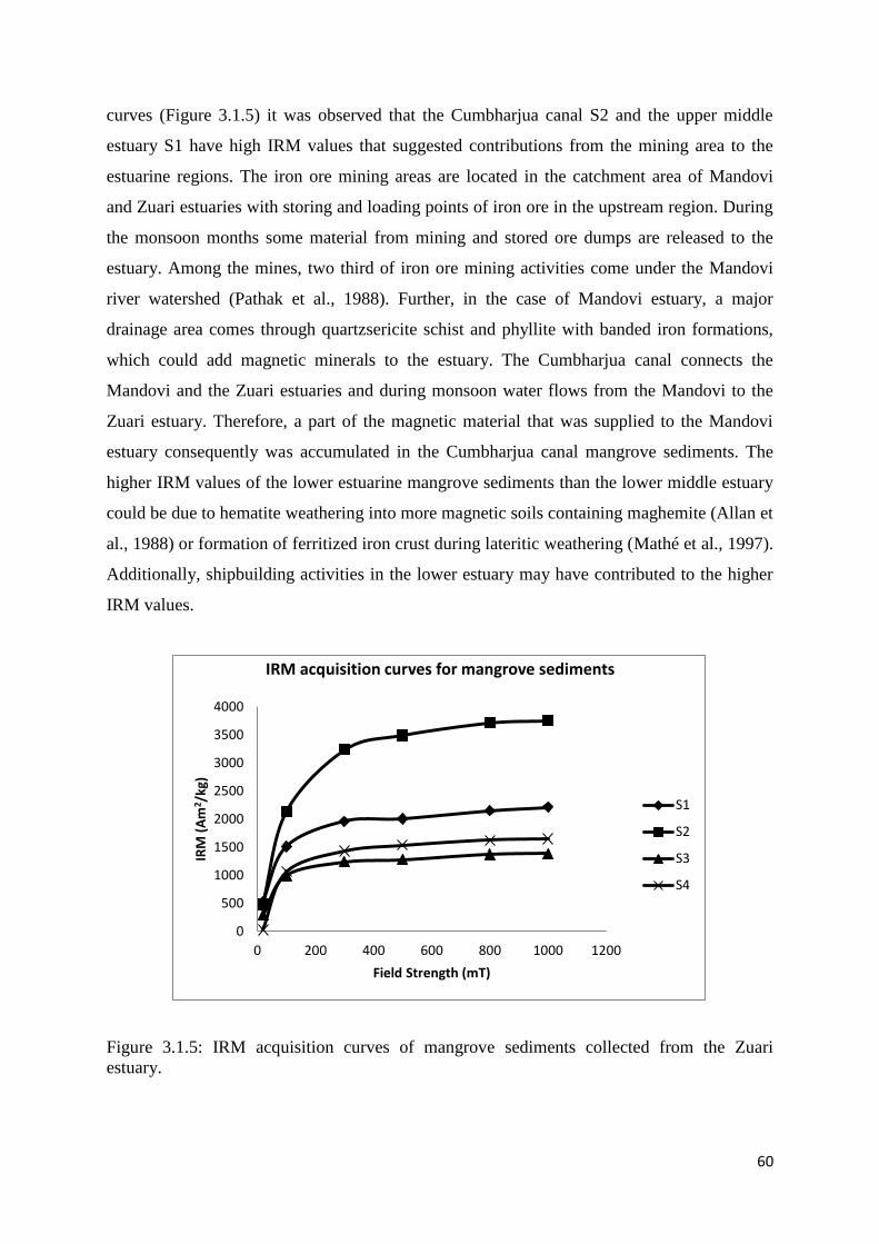
60
curves (Figure 3.1.5) it was observed that the Cumbharjua canal S2 and the upper middle
estuary S1 have high IRM values that suggested contributions from the mining area to the
estuarine regions. The iron ore mining areas are located in the catchment area of Mandovi
and Zuari estuaries with storing and loading points of iron ore in the upstream region. During
the monsoon months some material from mining and stored ore dumps are released to the
estuary. Among the mines, two third of iron ore mining activities come under the Mandovi
river watershed (Pathak et al., 1988). Further, in the case of Mandovi estuary, a major
drainage area comes through quartzsericite schist and phyllite with banded iron formations,
which could add magnetic minerals to the estuary. The Cumbharjua canal connects the
Mandovi and the Zuari estuaries and during monsoon water flows from the Mandovi to the
Zuari estuary. Therefore, a part of the magnetic material that was supplied to the Mandovi
estuary consequently was accumulated in the Cumbharjua canal mangrove sediments. The
higher IRM values of the lower estuarine mangrove sediments than the lower middle estuary
could be due to hematite weathering into more magnetic soils containing maghemite (Allan et
al., 1988) or formation of ferritized iron crust during lateritic weathering (Mathé et al., 1997).
Additionally, shipbuilding activities in the lower estuary may have contributed to the higher
IRM values.
Figure 3.1.5: IRM acquisition curves of mangrove sediments collected from the Zuari
estuary.
0
500
1000
1500
2000
2500
3000
3500
4000
0 200 400 600 800 1000 1200
IRM
(A
m2 /
kg)
Field Strength (mT)
IRM acquisition curves for mangrove sediments
S1
S2
S3
S4
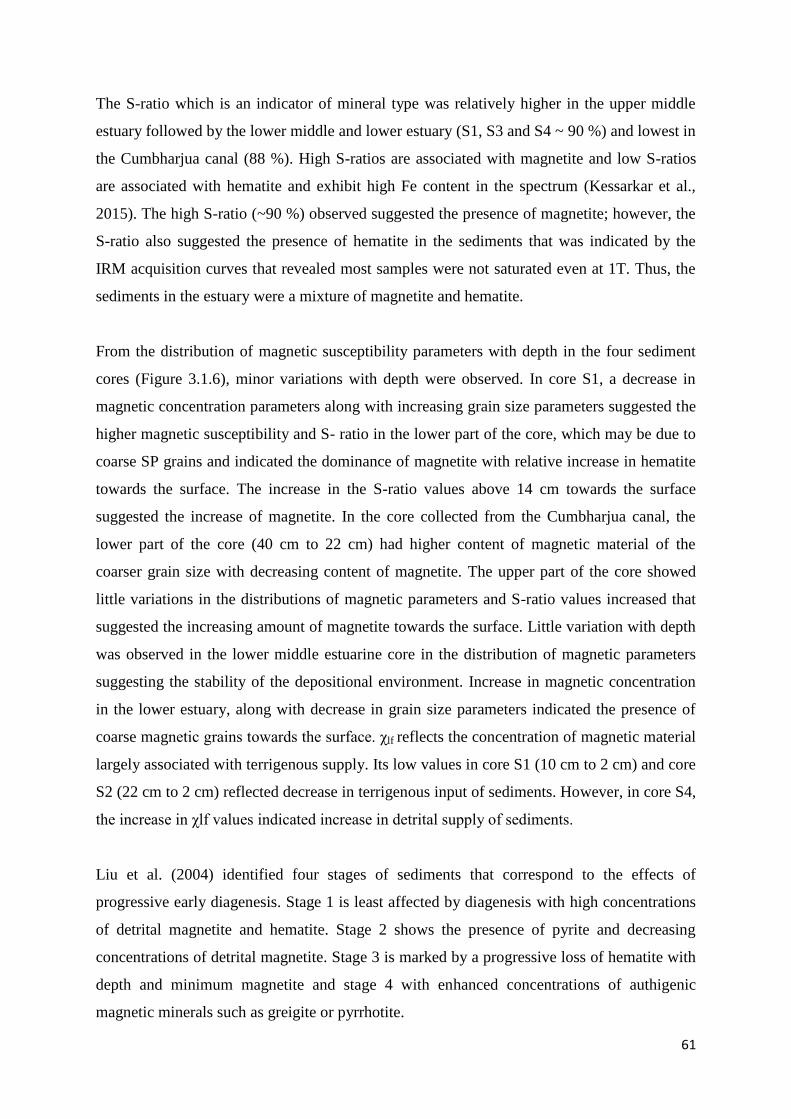
61
The S-ratio which is an indicator of mineral type was relatively higher in the upper middle
estuary followed by the lower middle and lower estuary (S1, S3 and S4 ~ 90 %) and lowest in
the Cumbharjua canal (88 %). High S-ratios are associated with magnetite and low S-ratios
are associated with hematite and exhibit high Fe content in the spectrum (Kessarkar et al.,
2015). The high S-ratio (~90 %) observed suggested the presence of magnetite; however, the
S-ratio also suggested the presence of hematite in the sediments that was indicated by the
IRM acquisition curves that revealed most samples were not saturated even at 1T. Thus, the
sediments in the estuary were a mixture of magnetite and hematite.
From the distribution of magnetic susceptibility parameters with depth in the four sediment
cores (Figure 3.1.6), minor variations with depth were observed. In core S1, a decrease in
magnetic concentration parameters along with increasing grain size parameters suggested the
higher magnetic susceptibility and S- ratio in the lower part of the core, which may be due to
coarse SP grains and indicated the dominance of magnetite with relative increase in hematite
towards the surface. The increase in the S-ratio values above 14 cm towards the surface
suggested the increase of magnetite. In the core collected from the Cumbharjua canal, the
lower part of the core (40 cm to 22 cm) had higher content of magnetic material of the
coarser grain size with decreasing content of magnetite. The upper part of the core showed
little variations in the distributions of magnetic parameters and S-ratio values increased that
suggested the increasing amount of magnetite towards the surface. Little variation with depth
was observed in the lower middle estuarine core in the distribution of magnetic parameters
suggesting the stability of the depositional environment. Increase in magnetic concentration
in the lower estuary, along with decrease in grain size parameters indicated the presence of
coarse magnetic grains towards the surface. χlf reflects the concentration of magnetic material
largely associated with terrigenous supply. Its low values in core S1 (10 cm to 2 cm) and core
S2 (22 cm to 2 cm) reflected decrease in terrigenous input of sediments. However, in core S4,
the increase in χlf values indicated increase in detrital supply of sediments.
Liu et al. (2004) identified four stages of sediments that correspond to the effects of
progressive early diagenesis. Stage 1 is least affected by diagenesis with high concentrations
of detrital magnetite and hematite. Stage 2 shows the presence of pyrite and decreasing
concentrations of detrital magnetite. Stage 3 is marked by a progressive loss of hematite with
depth and minimum magnetite and stage 4 with enhanced concentrations of authigenic
magnetic minerals such as greigite or pyrrhotite.

62

63
Figure 3.1.6: Distribution of magnetic susceptibility parameters with depth in cores mangrove
sediment cores S1, S2, S3, and S4.
A decreased peak of all the parameters, namely magnetic concentration, grain size and
mineralogy in sediments of core S1 at 14 cm indicated stage 2 diagenesis. High TOC at 14
cm may have favored reductive diagenesis and dissolution of magnetic minerals. The high S-
ratios in lower portion of the core and surface sediments indicated that the ferrimagnetic
material was the dominant component. The low values of χARM, χARM / χlf and χARM /SIRM at
10 cm indicated that the fine grained ferrimagnetic components are selectively dissolved
during early diagenesis (Karlin, 1990) leaving a residue of coarse grained lithogenic
magnetites (Rolph et al., 2004).
3.1.A.4 Geochemistry of sediments
3.1.A.4a Metals in bulk sediments
The range and average values of metals in the bulk sediments of mangrove cores S1, S2, S3
and S4 are presented in table 3.1.2.
The metal content in the sediment core S1 showed that major elements Al % varied from 7.28
% to 11.24 % (average 8.75 %), Fe % ranged from 9.26% to 12.47 % (average 10.84 %) and

64
Mn concentration varied between 4132 ppm and 6793 ppm (average 5181 ppm). Trace metals
Cr, Co, Ni, Cu and Zn ranged from 228 ppm to 405 ppm (average 274 ppm), 14.00 ppm to
27.75 ppm (average 21.75 ppm), 33.75 ppm to 58.00 ppm (average 41.78 ppm), 34.50 ppm to
59.25 ppm (average 45.9 ppm) and 122 ppm to 187 ppm (average 144 ppm ) respectively. In
sediment core S2 collected from the Cumbharjua canal, Al, Fe and Mn ranged from 6.64 % to
10.73 % (average 8.38 %), 11.20 % to 20.89 % (average 14.53 %) and 2049 ppm to 8134
ppm (average 5122 ppm) respectively. The trace metal concentrations of Cr, Co, Ni, Cu and
Zn ranged from 175 ppm to 428 ppm (average 271 ppm), 18.50 ppm to 30.75 ppm (average
22.85 ppm), 36.50 ppm to 73.75 ppm (average 47.15 ppm), 30.50 ppm to 50.00 ppm (average
36.26 ppm) and 85.50 ppm to 194 ppm (average104 ppm) respectively. The lower middle
estuarine sediment core S3 showed that, Al, Fe and Mn concentrations ranged from 10.28 %
to 15.80 % (average 11.59 %), 8.57 % to 12.10 % (average 10.54 %) and 1281 ppm to 4004
ppm (average 2138 ppm) respectively. Trace metals Cr, Co, Ni, Cu and Zn concentrations
ranged from 210 ppm to 494 ppm (average 318 ppm), 17.75 ppm to 27.75 ppm (average
23.23 ppm), 35.75 ppm to 49.50 ppm (average 44.33 ppm) , 33.50 ppm to 52.25 ppm
(average 42.11 ppm) and 117 ppm to 153 ppm (average 127 ppm) respectively. In the lower
estuarine core sediment S4, major elements Al, Fe and Mn ranged from 3.63 % to 9.94 %
(average 6.33 %), 7.25 % to 10.35 % (average 9.15 %) and 448 ppm to 2286 ppm (average
1153 ppm). Trace metals Cr, Co, Ni, Cu and Zn concentrations varied from 216 ppm to 542
ppm (average 336 ppm), 2.25 ppm to 29.50 ppm (average 19.98 ppm), 18.75 ppm to 39.50
ppm (average 27.6 ppm), 18.75 ppm to 37.75 ppm (average 26.92 ppm) and 46.25 ppm to
119.50 ppm (average 79.63 ppm).
The distribution of metals with depth in the four-mangrove sediment cores are presented in
figure 3.1.7. In the distribution of major and trace metals in core S1 with depth, Al showed a
near uniform distribution with minor increase from 34 cm to 12 cm followed by constant
distribution pattern toward the surface. Fe also exhibited a near uniform distribution with
minor positive peaks at 26 cm and negative peak at 24 cm. Mn concentrations decreased from
34 cm to 14 cm with a peak at 22 cm followed by constant distribution towards the surface.
Cr, Co, Ni, Cu, and Zn showed similar distribution trends to Fe with common peaks around
26 cm and 24 cm depth. The similar distribution trends of Cr, Co, Ni, Cu, and Zn with Fe
suggested the adsorption of metals onto Fe oxides. However, peak values at 10 cm for most
of the trace metals along with Mn indicated their diagenetic enrichment in the sedimentary
column. Co, Ni, Cu showed slightly increased concentrations at the surface.
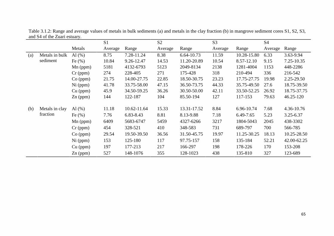
65
Table 3.1.2: Range and average values of metals in bulk sediments (a) and metals in the clay fraction (b) in mangrove sediment cores S1, S2, S3,
and S4 of the Zuari estuary.
S1 S2 S3 S4 Metals Average Range Average Range Average Range Average Range
(a) Metals in bulk
sediment
Al (%) 8.75 7.28-11.24 8.38 6.64-10.73 11.59 10.28-15.80 6.33 3.63-9.94
Fe (%) 10.84 9.26-12.47 14.53 11.20-20.89 10.54 8.57-12.10 9.15 7.25-10.35
Mn (ppm) 5181 4132-6793 5123 2049-8134 2138 1281-4004 1153 448-2286
Cr (ppm) 274 228-405 271 175-428 318 210-494 336 216-542
Co (ppm) 21.75 14.00-27.75 22.85 18.50-30.75 23.23 17.75-27.75 19.98 2.25-29.50
Ni (ppm) 41.78 33.75-58.00 47.15 36.50-73.75 44.33 35.75-49.50 27.6 18.75-39.50
Cu (ppm) 45.9 34.50-59.25 36.26 30.50-50.00 42.11 33.50-52.25 26.92 18.75-37.75
Zn (ppm) 144 122-187 104 85.50-194 127 117-153 79.63 46.25-120
(b) Metals in clay
fraction
Al (%) 11.18 10.62-11.64 15.33 13.31-17.52 8.84 6.96-10.74 7.68 4.36-10.76
Fe (%) 7.76 6.83-8.43 8.81 8.13-9.88 7.18 6.49-7.65 5.23 3.25-6.37
Mn (ppm) 6409 5683-6747 5459 4327-6266 3217 1804-5043 2045 438-3302
Cr (ppm) 454 328-521 410 348-583 731 689-797 700 566-785
Co (ppm) 29.54 19.50-39.50 36.56 31.50-45.75 19.97 11.25-30.25 18.13 10.25-28.50
Ni (ppm) 153 125-180 117 97.75-157 158 135-184 52.21 42.00-62.25
Cu (ppm) 197 177-213 217 166-297 198 178-226 170 153-208
Zn (ppm) 527 148-1076 355 128-1023 438 135-810 327 123-689

66

67
Figure 3.1.7: Distribution of bulk metals Fe, Mn, Cr, Co, Ni, Cu and Zn with depth in
mangrove sediment cores S1, S2, S3 and S4.
In core S2, when the distribution of metals was considered with depth, Al displayed a
constant distribution trend towards the surface with minor fluctuations around the average. Fe
and Mn showed resemblance in their distribution patterns with an increasing trend up to 22
cm followed by a decreasing trend towards the surface. The peaks at 30 cm and 24 cm in the
profiles of Fe and Mn suggested their diagenetic mobilization. Trace metals Cr, Co, Ni, Cu
and Zn exhibited high concentrations in the lower part of the core (54 cm to 46 cm) with
higher peak at 50 cm that agreed with Al and Fe. Cr, Ni, Cu and Zn showed slight increase
near the surface. The depth profile of metals in core S3 showed uniform distribution patterns
for major elements Al and Fe with depth. Mn increased between 12 cm to 0 cm indicating
recent inputs. Most of the trace metals Cr, Co, Ni, and Zn displayed uniform distribution
patterns with depth similar to Al and Fe. The concentration of Cu increased up to 14 cm from
the bottom of the core. Overall, no large variations in concentrations with depth were
observed except for Mn and Cu. Most of the metals showed a positive peak at 32 cm and
negative peak at 12 cm depth. The distribution of metals with depth in sediment core S4
showed that Al, Fe, and Mn concentrations increased towards the surface. Trace metals Cr,
Ni, Cu and Zn closely followed the distribution of Al, Fe and Mn in the vertical distribution
suggesting their association with aluminosilicates and Fe-Mn oxides.

68
Further, Pearson’s correlation analysis was carried out to understand the association of metals
with the sediment components to ascertain the factors that govern their distribution in the
sediments of the estuary and the results are presented in table 3.1.3. The range and average
values showed considerable spatial variations in the distribution of metals. High average
values of Mn, Cu, and Zn were noted in core S1, Fe and Ni in the core S2, Al and Co in core
S3 and Cr in core S4 sediments.
The trends and associations observed in the sediment cores indicated different sedimentary
processes operated at the four locations. In the upper middle estuary (S1), the highest
concentrations of Mn, Cu and Zn were noted which implied the proximity of their source to
the sampling location. The similar distribution trends of Cr, Co, Ni and Cu with Fe and their
positive correlation with sand suggested the formation of Fe oxides coating on the sand
particles. The trace metals must have adsorbed onto the Fe-oxide surfaces and/or may be
present as silicates in rock fragment or heavy minerals (d’Anglejan et al., 1990). Burdige
(1993) reported that iron and manganese oxides take up a variety of transition elements and
heavy metals, either by adsorption to the oxide surface or by direct incorporation into the
crystal structure. The distribution of Fe and Mn in estuarine sediments was affected by
variations in several physicochemical factors like salinity, pH, Eh along the estuary. Low
salinity in the upper reaches of the estuary must have caused the flocculation of Fe oxides
along with the adsorbed trace metals. All trace metals in core S1 showed poor correlation
with Al indicating their different source may be anthropogenic or different depositional
process. However, peak values of metals at 10 cm for most of the trace metals along with Mn
indicated their diagenetic re-mobilization in the sedimentary column (Jenne, 1968; Turekian,
1977). Thus, the distribution of most trace metals in this core was influenced by adsorption
onto Fe-oxides and flocculation in low salinity.
Highest concentrations of Fe and Ni were recorded in sediment core S2 collected from the
Cumbharjua canal. Mn in the Cumbharjua canal sediments was either associated with the silt-
sized particles or may have occurred in the form of detrital mining particles that was implied
by the significant correlation of Mn with silt. Further, Fe and Mn showed synchronous
distribution with depth in this core reflecting similarity in their redox behaviors and the peak
at 30 cm suggested their diagenetic enrichment. The high concentration of trace metals in the
lower part of the core (54 cm to 50 cm), along with Al, Fe and Mn peak indicated lithogenic
input. The significant association of Cr with Al and Fe implied a detrital source for Cr.

69
Table 3.1.3: Pearson’s correlation coefficients of sediment components and bulk metals of mangrove cores S1 (a), S2 (b), S3 (c) and S4 (d) of
the Zuari estuary.
(a) Correlations-S1
pH Sand Silt Clay TOC Al Fe Mn Cr Co Ni Cu Zn
pH 1.00
Sand -0.04 1.00
Silt 0.07 -0.45 1.00
Clay -0.07 0.21 -0.97** 1.00
TOC 0.65** -0.11 -0.11 0.15 1.00
Al 0.19 -0.56 0.07 0.08 0.26 1.00
N=17
Fe -0.19 0.59* -0.13 -0.03 -0.23 -0.04 1.00
Mn 0.09 -0.15 0.26 -0.24 -0.28 0.00 -0.01 1.00
Cr -0.11 0.39 -0.24 0.15 -0.22 -0.10 0.53* 0.00 1.00
Co 0.15 0.49* 0.05 -0.20 0.11 -0.06 0.59* 0.12 0.18 1.00
Ni -0.08 0.38 -0.19 0.10 -0.17 0.00 0.31 -0.29 -0.22 0.27 1.00
Cu 0.10 0.69** -0.16 -0.02 -0.18 -0.49* 0.53* 0.10 0.70** 0.39 -0.03 1.00
Zn -0.53** 0.12 -0.03 0.00 -0.68** -0.05 0.37 -0.10 0.02 0.05 0.52* -0.01 1.00
Correlations- S2 (b) pH Sand Silt Clay TOC Al Fe Mn Cr Co Ni Cu Zn
pH 1.00
Sand 0.10 1.00
Silt -0.16 -0.44* 1.00
Clay 0.15 0.18 -0.96** 1.00
TOC 0.42* 0.00 0.32 -0.35 1.00
Al 0.11 0.05 0.05 -0.07 0.22 1.00
N=27
Fe -0.50** -0.23 0.16 -0.11 -0.14 0.32 1.00
Mn -0.32 -0.52** 0.58** -0.47* -0.12 -0.03 0.41* 1.00
Cr -0.11 0.19 -0.14 0.09 -0.19 0.52** 0.42* -0.08 1.00
Co -0.18 0.29 -0.15 0.08 -0.03 -0.03 0.18 0.04 0.16 1.00
Ni 0.11 0.30 -0.64** 0.61** -0.08 -0.12 -0.10 -0.30 0.24 0.36 1.00
Cu -0.10 0.15 -0.34 0.33 -0.03 0.00 0.35 -0.26 0.49* 0.56** 0.65** 1.00
Zn 0.15 0.24 -0.26 0.21 0.08 0.02 -0.17 -0.25 0.37 0.59** 0.66** 0.69** 1.00

70
Correlations-S3 (c) pH Sand Silt Clay TOC Al Fe Mn Cr Co Ni Cu Zn
1.00
Sand 0.39 1.00
Silt -0.42 -0.02 1.00
Clay 0.40 -0.04 -1.00** 1.00
TOC -0.19 -0.07 0.16 -0.15 1.00
Al -0.08 -0.14 0.39 -0.39 0.47* 1.00
Fe -0.28 -0.12 0.34 -0.33 0.27 0.58** 1.00
N=20
Mn 0.13 0.01 0.06 -0.06 -0.60** -0.36 -0.02 1.00
Cr -0.12 -0.14 0.42 -0.41 0.23 0.80** 0.63** -0.17 1.00
Co -0.40 0.12 0.33 -0.34 0.02 0.12 0.46* 0.22 0.34 1.00
Ni -0.20 0.14 0.35 -0.36 0.03 0.19 0.49* 0.27 0.24 .510* 1.00
Cu -0.13 0.15 0.34 -0.35 -0.11 0.37 0.65** 0.18 0.66** 0.66** 0.34 1.00
Zn -0.29 -0.04 0.53* -0.53* 0.26 0.69** 0.83** 0.07 0.78** 0.59** 0.45* 0.82** 1.00
(d) Correlations- S4
pH Sand Silt Clay TOC Al Fe Mn Cr Co Ni Cu Zn
1.00
Sand -0.34 1.00
Silt 0.18 -0.95** 1.00
Clay 0.51 -0.90** 0.72** 1.00
TOC 0.49 -0.86** 0.82** 0.77** 1.00
Al 0.29 -0.91** 0.91** 0.75** 0.82** 1.00
N=12
Fe 0.13 -0.55 0.44 0.62* 0.45 0.62* 1.00
Mn 0.38 -0.90** 0.90** 0.74** 0.83** 0.98** 0.49 1.00
Cr -0.15 -0.59* 0.63* 0.42 0.52 0.77** 0.79** 0.65* 1.00
Co -0.10 -0.19 0.35 -0.06 0.30 0.44 -0.04 0.49 0.25 1.00
Ni 0.40 -0.83** 0.82** 0.71* 0.71** 0.91** 0.46 0.91** 0.53 0.45 1.00
Cu 0.55 -0.86** 0.78** 0.83** 0.76** 0.87** 0.59* 0.86** 0.50 0.31 0.93** 1.00 Zn 0.44 -0.90** 0.87** 0.80** 0.85** 0.96** 0.60* 0.95** 0.72** 0.26 0.85** 0.86** 1.00
71
However, the similar distribution trends of Co, Ni, Cu and Zn and their significant correlation
implied a common source for these metals that may be anthropogenic. It is important to note
that substantial amount of material from the Mandovi River is added to the Zuari via the
Cumbharjua canal. Singh et al. (2013) previously reported high concentrations of trace metals
in mudflats of the Zuari estuary in the upper middle and Cumbharjua canal sediments, which
they have interpreted as due to the effects of the nearby mining zones and ore transportation
by barges. Further, they stated that increased accumulation of Fe and Mn in the upper middle
estuary and Cumbharjua canal can considerably trap trace metals that can cause damage to
the sediment quality.
The lower middle estuary (S3) showed little variations in metal distribution patterns and
sediment grain size suggesting not much change in sediment and metal input with time. At
this location, the canal joins the Zuari estuary and facilitates mixing of the two waters and
sediment. Metals associated with suspended matter may have been fully mixed and then
deposited in this area thus showed the uniform distribution in the depth profiles. Zhou et al.
(2004) reported similar observation earlier. The increasing trend of Mn in this core suggested
recent input probably of anthropogenic origin. The similar distribution pattern and good
correlation indicated that metals Cr, Co, Ni, Cu and Zn were associated with Fe oxides in the
sediments. Cr and Zn, however, showed association with Al, thus indicating a lithogenic
source.
Further, most of the studied metals were less concentrated at the lower estuary (S4). Mistch et
al. (2009) and Sun et al. (2015) stated that the sites that are subjected to intensive tidal
washing generally have lower metal concentrations, while those subjected to relatively lower
energy facilitated the deposition of metal particles. In the lower estuary core, the metals were
associated with the finer sediments, TOC, Al, Fe, and Mn that suggested their lithogenic
source. The low concentration of metals towards the base of the core can be related to the
dilution of metals by coarser sediments.
The comparison of bulk metals and clay minerals profiles revealed that in core S1 the
distribution to Cr showed similar to chlorite whereas Ni showed similar to kaolinite. Zinc
exhibited similar to smectite in core S2. Metals showed little association with the clay
minerals in cores S3 and S4. Albee (1962) reported that in natural chlorites, small amounts of
Cr do substitute Si. Mattigod et al. (1979) studied the adsorption of Ni onto kaolinite and

72
found that increasing ionic strength decreased adsorption of Ni. Thus, the low salinity in the
upper middle estuary must have facilitating the adsorption of Ni onto kaolinite as compared
to the other locations in the estuary. Further, Zinc has a high affinity to adsorb onto clay
minerals due to its high ionic potential. The adsorption of Zn onto smectite was therefore,
thought to occur since the swelling of smectite allows greater access to interlayer sites.
Additionally, Aluminum ions are replaced from the octahedral interstices by zinc to form
sauconite, a type of smectitic clay (Kolay, 2007).
Further, the distribution of metals with depth was compared with magnetic susceptibility
parameters in the mangrove sediments. In core S1, Fe and Mn exhibited similar distribution
with the magnetic concentration parameters suggesting the source of Fe and Mn may be
anthropogenic, probably from active mining and transport of ferromanganese ores in the
upstream regions of the Zuari estuary. In core S2, Fe and Mn showed similar distribution
with magnetic grain size parameters with a peak at 22 cm, indicating that these metals were
anthropogenically influenced by mining inputs. The trace metals Cr, Co, Cu, Zn and to some
extent Ni in core S2 showed similarity to the magnetic grain size and mineralogy parameters
from 40 cm to 22cm and may have been associated with the coarse grain size. In core S3, no
significant association of metals along with the magnetic parameters was observed. In core
S4, Fe, Mn, Cr, Ni, Cu and Zn showed similar distribution pattern to the magnetic
concentration parameters that suggested that these metals have some anthropogenic influence
and are probably associated with Fe-oxides. The iron ore mined in the catchment areas and
transported contribute significantly to the ferrimagnetic particles of sediments resulting in
enhancement of magnetic susceptibility.
The similar distribution profiles between magnetic parameters and metal concentrations
revealed an understandable relation between ferrimagnetic oxides and metals. Previous
studies by Schmidt et al. (2005) indicated that the correlation between magnetic susceptibility
and metal contamination only exists for the polluted samples, like those that carry magnetic
inclusions. Since the magnetic susceptibility of the sediments was mainly influenced by iron
oxides, the association of the trace metals with these iron oxides could result in association of
the metals with the magnetic parameters. Magnetic particles, in the form of fine iron oxide
dusts, could have been released along with other metals from a combination of different
sources and introduced into the sediments (Lu et al., 2007) and the reduction of these iron
oxides can have direct influence on the recycling of metals (Burdige, 1993). Fine grains that

73
are known to have a high surface to volume ratio are sensitive to the active sites of iron
oxides. The grain size and hence the surface area thus influence the kinetics and extent of
iron oxide dissolution and mobilization of associated trace metals in sediments (Roden and
Zachara, 1996; Haese et al., 1997, Dessai and Nayak, 2007). Additionally, magnetic grain
size parameters did not show association with the metal concentrations indicating association
of metals towards the coarser magnetic grains. Thus, the comparison between magnetic
susceptibility and metal distributions indicated the role played by particle size and iron oxide
in the distribution of metals.
3.1. A.4b Metals in the clay fraction of sediments
To understand the distribution of metals in the clay fraction of sediments, the clay fraction
was separated for analysis as clay has a strong tendency to adsorb trace metals. Analysis of
metals Al, Fe, Mn, Cr, Co, Ni, Cu and Zn in clay fraction was carried out for selected
samples of the four mangrove cores and the range and average values are presented in table
3.1.2 (b). In sediment core S1, Al, Fe and Mn concentrations ranged from 10.62 % to 11.64
% (average 11.18 %), 6.83 % to 8.43 % (average 7.76 %) and 5683 ppm to 6747 ppm
(average 6409 ppm). The trace metals Cr, Co, Ni, Cu and Zn concentrations varied from 328
ppm to 521 ppm (average 454 ppm), 19.50 ppm to 39.50 ppm (average 29.54 ppm), 125 ppm
to 180 ppm (average 153 ppm), 177 ppm to 212 ppm (average 197 ppm) and 148 ppm to
1076 ppm (average 527 ppm). In sediment core S2 collected from the Cumbharjua canal, Al,
Fe and Mn content ranged from 13.31 % to 17.52 % (average 15.33 %), 8.13 % to 9.88 %
(average 8.81 % ), 4327 ppm to 6265 ppm (average 5459 ppm) respectively. The trace metals
Cr, Co, Ni, Cu and Zn concentrations ranged from 348 ppm to 583 ppm (average 410 ppm),
31.50 ppm to 45.75 ppm (average 36.56 ppm), 97.75 ppm to 157 ppm (average 117 ppm) ,
166 ppm to 297 ppm (average 217 ppm) and 128 ppm to 1025 ppm (average 355 ppm)
respectively. Metals in the lower middle estuary core S3 showed that Al, Fe and Mn
concentrations ranged from 6.96 % to 10.74 % (average 8.84 %), 6.49 to 7.65 % (average
7.18 %) and 1804 ppm to 5043 ppm (average 3217 ppm) respectively. Trace metal
concentrations in the clay fraction of Cr, Co, Ni, Cu and Zn ranged from 689 ppm to 797
ppm (average 731 ppm), 11.25 ppm to 30.25 ppm (average 19.97 ppm), 135 ppm to 184
ppm (average 158 ppm), 178 ppm to 226 ppm (average 198 ppm) and 135 ppm to 810 ppm
(average 438 ppm). The sediment core collected from the lower estuary S4, showed major
metals Al, Fe and Mn in the clay fraction of sediments to range from 4.36 % to 10.76 %
(average 7.68 %), 3.25 % to 6.37 % (average 5.23 %) and 440 ppm to 3302 ppm (average

74
2045 ppm). Trace metals Cr, Co, Ni Cu and Zn in the clay fraction of sediments ranged from
566 ppm to 785 ppm (average 700 ppm), 10.25 ppm to 28.50 ppm (average 18.13 ppm),
42.00 ppm to 62.25 ppm (average 52.21 ppm), 153 ppm to 208 ppm (average 170 ppm) and
123 ppm to 689 ppm (average 327 ppm).
The highest concentrations of Al, Fe, Co and Cu were observed in core S2; Cr, Ni and Zn in
core S3 and Mn in core S1.

75
Figure 3.1.8: Distribution of metals in the clay fraction of sediments in mangrove cores S1,
S2, S3 and S4.
From the distribution of metals in the clay fraction with depth presented in figure 3.1.8, metal
distribution in core S1 revealed that Al showed a constant distribution trend with depth. Fe,
Mn and Cu concentrations decreased towards the surface while Cr, Ni and Zn showed similar
distribution trends with a decrease from the base of the core to around 22 cm followed by a
peak at around 14 cm, and Co fluctuated in its distribution with a peak at 18 cm followed by
higher concentration towards the surface. Overall, the lower portion of the core had high
concentrations for most metals. The minor decrease in the Mn profile at 14 cm and increase
around 10 cm suggested the diagenetic enrichment of Mn, similar to its distribution in the
76
bulk sediments. The distribution of the metals in the clay fraction with depth in core S2
revealed that the Al distribution showed a peak at 18 cm followed by decrease towards the
surface. Cr, Co, Ni and Zn showed similar distribution to the profile of Fe suggesting that Fe
oxides played a major role in their distribution. Mn concentrations gradually increased
towards the surface whereas Cu showed a fluctuating increase towards the surface. In the
distribution of metals in the clay fraction with depth in core S3, Al, Fe and Mn concentrations
gradually increased towards the surface. Cr concentration decreased whereas Co, Ni, Cu and
Zn showed similar distribution profiles with a common peak at 18 cm. The distribution of
metals in the clay fraction of sediments with depth of the lower estuary mangrove core S4
exhibited an increase in Cr, Co, Ni and Cu towards the surface. Al, Fe and Mn increased up
to 10 cm and then showed gradual decrease towards the surface. Zn showed constant value up
to 18 cm followed by sharp decrease up to 14 cm and then gradual increase towards the
surface.
In the core collected from the upper middle estuary, Fe exhibited similar distribution to Al
with depth and Ni similar to Zn indicating that they are derived from a common source. Trace
metals, Cr, Co, Ni and Zn in the Cumbharjua canal showed similar distribution to Fe and
indicated that Fe oxides strongly influenced the distribution of Cr, Co, Ni and Zn and were
derived from a common source. Further, the similar distribution of Al, Fe and Mn in the
lower middle estuary core indicated natural source whereas the similar distributions of Co,
Ni, Cu and Zn suggested a common source for these metals and were probably of detrital
nature. In core collected from the lower estuary the similar distribution of trace metals Cr,
Co, Ni and Cu indicated that the metals were derived from a common source whereas Zn may
have been derived from a different source.
The average concentrations of metals in the clay fraction (table 3.1.2) were compared with
the bulk metals using the Isocon diagram (Grant, 1986) presented in figure 3.1.9.
In core S1 and core S2, all metals showed higher concentrations in the clay fraction except
for Fe. Further, in core S3, Al, Fe and Co showed higher concentrations in the bulk and other
metals were higher in the clay fraction. Fe and Co in sediment core S4 showed higher
concentrations in the bulk suggesting their association with the larger sized sediments.
Volvoikar and Nayak (2014) reported that the clay-sized fraction of sediments represents last
and stable weathering product of strong erosion of source rocks and holds metals within the

77
lattice structure of aluminosilicate minerals. The high content of Fe in the bulk sediments
indicated Fe association with larger sediment particles like sand and silt (Roussiez et al.,
2006).
Figure 3.1.9: Isocon diagram of metals in bulk sediments versus metals in clay fraction in
mangrove cores S1, S2, S3 and S4.
3.1.B Mudflats
Three mudflat cores were collected from the Zuari estuary, one each from the upper middle
estuary M1, lower middle estuary M3 and lower estuary M4. The cores were analyzed for
sediment components, clay mineralogy, magnetic susceptibility and metal chemistry and the
results are presented in the following sections.
3.1. B.1 Sediment components (pH, sand, silt, clay and total organic carbon)
The range and average values of sediment components of mudflat cores are presented in table
3.1.4 (a).

78
Table 3.1.4: Range and average values of sediment components, clay mineralogy, and magnetic susceptibility parameters in mudflat cores M1,
M3, and M4 of the Zuari estuary.
M1 M3 M4 Parameters Average Range Average Range Average Range
pH 6.87 6.47-7.34 7.05 6.78-7.38 7.24 7.00-7.43 (a) Sediment
components
Sand (%) 2.52 1.07- 8.55 1.62 0.35 -8.42 9.79 4.75- 16.51
Silt (%) 40.1 24.93 -47.41 34.47 23.56 -41.66 40.66 34.04 -47.55 Clay (%) 57.38 49.52-64.52 63.91 49.92 -75.92 49.55 42.84 - 57.36 TOC (%) 2.58 1.79-3.10 2.48 2.18-2.94 2.01 1.71 -2.43 (b) Clay minerals Smectite (%) 15.93 10.87 -18.80 16.19 11.11-20.00 31.83 17.87 - 50.00
Illite (%) 20.86 16.67- 23.93 21.12 17.50- 24.00 18.85 7.92 - 25.00 Kaolinite (%) 56.67 51.24- 62.21 55.37 51.99- 62.02 45.03 20.31- 62.34 Chlorite (%) 6.54 4.34- 9.63 7.32 3.61 -12.43 4.29 2.70 - 5.67 (c) Magnetic
Susceptibility
parameters
χlf (10-8
m3 kg
-1) 229 200 - 273 159 139 -169 172 136 - 194
χARM (10-8
m3 kg
-1 ) 1135 1086-1281 1025 925 - 1092 942 794- 1040
SIRM (10-5
Am2
kg-
1)
2090 1723 - 2669 1402 1360 -1465 1839 1522- 2186 χARM/χlf 5.02 4.09-5.53 6.44 6.13 - 6.76 5.49 5.1- 5.84 χARM/SIRM (10
-3 A
-
1m )
0.55 0.41-0.64 0.73 0.67- 0.78 0.52 0.46- 0.60 χ fd (%) 6.24 4.04- 7.67 7.59 2.68 -9.76 6.60 2.22-12.40 S-ratio (%) 89.73 87.50-91.99 89.87 87.78 - 92.59 90.22 85.69-92.74

79
In the sediment core collected from the upper middle estuary (M1) representing the mudflat
environment, the pH was near neutral in nature and ranged from 6.47 to 7.34 (average 6.87).
The sediments showed that sand, silt and clay content ranged from 1.07 % to 8.55 % (average
2.52 %), 24.93 % to 47.41 % (average 40.1 %) and 49.52 % to 64.52 % (average 57.38 %)
respectively. The TOC content in the mudflat core M1 ranged from 1.79 % to 3.10 %
(average 2.58 %). The variation in sediment components in the lower middle estuarine
region (M3) showed that the pH was near neutral and ranged from 6.78 to 7.38 (average
7.05). The sand, silt and clay content in mudflat core M3 varied from 0.35 % to 8.42 %
(average 1.62 %), 23.56 % to 41.66 % (average 34.47 %) and 49.92 % to 75.92 % (average
63.91 %) respectively. TOC in core M3 ranged from 2.18 % to 2.94 % (average 2.48 %).
Figure 3.1.10 Distribution of sediment components with depth in mudflat sediments of core
M1, M3 and M4.
In the mudflat core collected from the lower estuary (M4). The pH was weakly alkaline
ranging from 7.00 to 7.43 (average 7.24). The sand, silt and clay percentages ranged from

80
4.75 % to 16.51 % (average 9.79 %), 34.04 % to 47.55 % (average 40.66 %) and 42.84 % to
57.36 % (average 49.55 %). The TOC content in the core ranged from 1.71 % to 2.43 %
(average 2.01 %).
The distribution of sediment components with depth in cores M1, M3 and M4 are presented
in figure 3.1.10. In the vertical profile of sediment components of core M1, the pH was
relatively constant with depth except for a few higher values in the lower portion of the core
(44 cm to 38 cm). Sand exhibited a uniform distribution pattern throughout the core with the
exception of higher sand percentages in the lower part of the core (44 cm to36 cm). Silt and
clay showed a complementary distribution pattern wherein silt percentage increased up to 28
cm and clay decreased up to 28 cm followed by a fluctuating distribution towards the surface.
TOC showed a gradual increase towards the surface and showed some similarity to the
distribution of silt. Overall clay was the dominant grain size over sand and silt. From the
distribution of sediment components with depth in core M3, pH was noted to be constant with
depth. Sand exhibited higher percentages in the lower portion of the core (42 cm to 40 cm)
followed by uniform distribution towards the surface. Silt and clay exhibited complementary
distribution patterns, with large fluctuations in their profiles, especially between 42 cm to 24
cm. This was followed by a decrease in silt percentage above 24 cm, which was compensated
by an increase in clay percentage towards the surface. The TOC percentages were almost
constant with depth with slightly higher percentages than average between 28 cm and 14 cm.
Overall, the core was dominated by clay. The distribution of sediment components in mudflat
core M4 with depth revealed that the distribution of pH in the core was relatively constant.
The sand content gradually decreased towards the surface, which was compensated by an
increase in silt content. The distribution of clay showed an opposite distribution to silt with
large fluctuations. The TOC content showed a minor increase towards the surface above the
average line and was largely associated with silt.
The range and average values revealed that the pH values recorded were among the normal
range values for estuarine sediments i.e. between 5 to 7 (Caçador et al., 2004; Reddy and
DeLaune, 2008). Higher pH was recorded in the lower estuary, which decreased towards the
upper middle estuary due to the decreasing tidal influence towards the upstream regions. The
average pH values at all stations were noted to be near neutral (7.0) which was also observed
by Spetter et al. (2014) particularly in non-vegetated sediments. The mudflat sediments along
the estuary were dominated by silt and clay. The lower estuary sediments had higher

81
percentage of sand and silt content whereas higher clay was noted in the lower middle
estuary. The lower estuary is subjected to high hydrodynamics due to turbulence by waves
that cause resuspension of the finer sediments, which are carried in suspension retaining the
larger sediment size fractions. Activities by waves are controlled by wind direction and
intensity, the water level on the mudflat, and the sediment characteristics (Deloffre et al.,
2007). In all the three mudflat cores, higher sand content was noted in the lower portion of
the cores, which indicated a higher energy regime prevailed during the deposition of the
sediments in the past.
Highest TOC values were recorded in the upper middle estuary M1 that may be related to the
high content of finer sized sediments or inputs from sewage and waste water on considering
the proximity of the sampling location to a ship building industry. In addition, as the upper
middle estuary has lower hydrodynamics, organic matter dissolution rates may have been
lower. Organic matter is supplied to the environments from both external (i.e. terrestrial,
agricultural domestic and municipal sewage) and internal (i.e. algal and microbial) sources.
Benthic invertebrates and microorganisms may also contribute significant amounts of organic
carbon to sediments (Reddy and DeLaune, 2008). In the core collected from the upper middle
estuary, similarity of the profiles of TOC with silt suggest increasing loads of silt deposited
with higher sedimentation rates must have trapped the higher TOC (Carreira et al., 2002).
Finer sediments have large surface areas and tend to have associated negative charges.
Therefore, on interacting with seawater, their surfaces are quickly coated with a layer of
organic material (Rojas and Silva, 2005). The core collected from the lower middle estuary
exhibited large fluctuations in the silt and clay profile suggesting prevailed varying
depositional conditions. The profile of TOC was similar to that of clay indicating the
association of organic matter with the fine sediment. In the core collected from the lower
estuary, the decreasing sand content towards the surface indicated calm conditions in recent
times with increase in the fine sediments and TOC.
Furthermore, by using the ternary diagram of Pejrup (1988), an understanding of the
depositional conditions was attempted for the three mudflat cores (Figure 3.1.B.2). The
sediments of mudflat cores M1 and M3 fell in class II (D) indicating relatively calm
hydrodynamic conditions prevailed during sediment deposition. The sediments of core M4
however fell in class II (C), II (D) and III (D) indicating varying hydrodynamic conditions
during deposition.

82
Figure 3.1.11 Ternary diagram proposed by Pejrup (1988) of sand, silt and clay of mudflat
cores M1, M3 and M4.
3.1.B.2 Clay mineralogy
Smectite, illite, kaolinite and chlorite comprised the clay mineral assemblage of the mudflat
sediments and the ranges and average values are presented in table 3.1.4 (b).
In the mudflat core M1, smectite, illite, kaolinite and chlorite percentages ranged from 10.87
% to 18.80 % (average 15.93 %), 16.67 % to 23.93 % (average 20.86 %), 51.24 % to 62.21 %
(average 56.67 %) and 4.34 % to 9.63 % (average 6.54 %), respectively. In core M3 collected
from the lower middle estuary, clay mineral percentages of smectite, illite, kaolinite and
chlorite ranged from 11.11 % to 20.00 % (average 16.19 %), 17.50 % to 24.00 % (average
21.12 %), 51.99 % to 62.02 % (average 55.37 %) and 3.61 % to 12.43 % (average 7.32 %)
respectively. The percentages of smectite, illite, kaolinite and chlorite in the core collected
from the lower estuary M4, ranged from 17.87 % to 50.00 % (average 31.83 %), 7.92 % to

83
25.00 % (average 18.85 %), 20.31 % to 62.34 % (average 45.03 %) and 2.70 % to 5.67 %
(average 4.29 %) respectively.
In the distribution profiles of clay minerals with depth (Figure 3.1.12), of core M1, all the
clay minerals showed a near uniform distribution profiles with minor fluctuations at 22 cm.
Smectite and illite showed similar distribution patterns, with minor decreased peak at 14 cm.
Kaolinite exhibited an opposite distribution pattern to smectite and illite. Chlorite showed a
positive peak at 14 cm depth. Little variations with depth were observed in the distribution
clay minerals in core M3 with depth. Smectite percentages were relatively constant with
depth except between 10 cm to 2 cm wherein a peak was observed at 6 cm. Illite percentage
showed minor fluctuations around the average line while kaolinite exhibited an opposite
distribution trend to smectite. Chlorite however, showed large variation in its distribution
wherein percentages increased from the base of the core up to 18 cm followed by decrease
towards the surface, except it showed an increase at the surface. The distribution of clay
minerals with depth in mudflat core M4 exhibited large fluctuations and opposite trends for
smectite and kaolinite. Smectite increased between 30 cm to 10 cm (except at 18 cm)
followed by a decrease towards the surface whereas kaolinite decreased up to 10 cm and then
increased. Illite percentages decreased towards the surface whereas chlorite percentage was
constant with depth.
Kaolinite was the most abundant clay mineral in the Zuari estuary followed by illite, smectite
and chlorite, except for the lower estuary where smectite was higher than illite. Kaolinite
was enriched in the upper middle estuary whereas smectite was high in the lower estuary and
illite and chlorite were abundant in the lower middle estuary. The transport and deposition of
sediments in estuaries are complex processes with various interacting factors affecting the
fate of the sediments. Clay minerals in estuary may be derived from weathering profiles on
the continents called detrital clays or they may be formed during and after deposition known
as diagenetic clays. Meade (1972) proposed three influencing factors that govern the
distribution of clay minerals, (i) dynamic processes that circulate and mix estuarine waters,
(ii) the flocculation process which increases the settling velocities of sediment particles, and
(iii) properties of the particles themselves. The precipitation of clay minerals mainly depends
on the flocculation, so the crystal habit of the clay minerals and geochemical environment of
the depositional region are also important factors affecting the distribution of clay minerals
(Yang, 1988).

84
Figure 3.1.12 Distribution of clay minerals with depth in mudflat sediments of cores M1, M3
and M4.
Studies by Edzwald and O'Melia (1975) reported that illite is more stable than kaolinite so
that under similar physical conditions, illite would be expected to aggregate more slowly than
kaolinite and be deposited downstream of kaolinite. For any given salinity, the fresh water
sediment is relatively unstable compared to downstream sediments. The lower estuary
sediment is more stable than the upper estuary sediment which is more stable than the fresh
water sediment. The clay deposited upstream undergone particle aggregation more rapidly
than those deposited downstream. Those clays, which are relatively stable will be transported
farther downstream due to slow aggregation rates before deposition can occur. As kaolinite is
less stable than illite and smectite, it was deposited towards the upstream region of the
estuary and hence explains the spatial variability in the abundance of the clay minerals.

85
Abundant smectite towards the lower estuary may have been transported from offshore
regions into the estuary.
The vertical distribution of clay minerals in the mudflats of the upper middle and lower
middle estuary revealed minor variations with depth that suggested little change in
provenance over time. The lower estuary however, showed large variations in the clay
mineral distributions mainly with respect to kaolinite and smectite that show opposite
distribution patterns. The increase in smectite and peak at 10 cm in the mudflat core of the
lower estuary suggested an increased seawater intrusion that transported large amount
smectite into the estuary. As mudflats are more in contact with the water as compared to
other intertidal sedimentary environments, the mudflats are more sensitive to the changes in
flux of material and provide a more accurate record of the prevailing environmental
conditions.
3.1.B.3 Magnetic susceptibility
The range and average values of magnetic susceptibility parameters of the mudflat cores M1,
M3 and M4 are presented in table 3.1.4(c). The magnetic mineral concentration parameters χlf
,values of the mudflat core M1 collected from the upper middle estuarine mangroves
markedly varied from 200 ×10-8
m3
kg-1
to 273 ×10-8
m3
kg-1
(average 229×10-8
m3
kg-1
), χARM
values ranged from 1085 ×10-8
m3
kg-1
to 1281 ×10-8
m3
kg-1
(average 1135 ×10-8
m3
kg-1
) and
SIRM values ranged from 1723 ×10-5
Am2 kg
-1 to 2669 ×10
-5 Am
2 kg
-1 (average of 2090 ×10
-
5 Am
2 kg
-1). The inter-parametric ratios of χARM / χlf, χARM /SIRM and χfd, that are indicative
of magnetic grain size ranged from 4.09 to 5.53 (average of 5.02), 0.41×10⁻³
A-1
m to
0.64×10⁻³
A-1
m (average of 0.55×10⁻³
A-1
m) and 4.04 % to 7.67 % (average 6.24 %)
respectively. The S-ratio % of core M1 ranged from 87.50 % to 91.99 % (average 89.73 %).
In the lower middle estuary mudflat core M3, χlf ,values ranged from 139 ×10-8
m3
kg-1
to
169 ×10-8
m3
kg-1
(average 159×10-8
m3
kg-1
), χARM values ranged from 925 ×10-8
m3
kg-1
to
1092 ×10-8
m3
kg-1
(average 1025×10-8
m3
kg-1
) and SIRM values ranged from 1360×10-5
Am2 kg
-1 to 1464 ×10
-5 Am
2 kg
-1 (average of 1402×10
-5 Am
2 kg
-1). The magnetic grain size
parameters of χARM / χlf, χARM /SIRM and χfd, ranged from 6.13 to 6.76 (average of 6.44),
0.67×10⁻³
A-1
m to 0.78×10⁻³
A-1
m (average of 0.73×10⁻³
A-1
m) and 2.68 % to 9.76 %
(average 7.59 %) respectively. The S-ratio % of core M3 ranged from 87.78 % to 92.59 %
(average 89.87 %). The core M4 of the mudflat environment of the lower estuary showed
that the concentration of magnetic material parameters χlf, χARM and SIRM ranged from 136
86
×10-8
m3
kg-1
to 194 ×10-8
m3
kg-1
(average 172×10-8
m3
kg-1
), χARM values ranged from 794
×10-8
m3
kg-1
to 1041×10-8
m3
kg-1
(average 942×10-8
m3
kg-1
) and SIRM values ranged from
1522×10-5
Am2 kg
-1 to 2186 ×10
-5 Am
2 kg
-1 (average of 1839×10
-5 Am
2 kg
-1). The magnetic
grain size parameters of χARM / χlf, χARM /SIRM and χfd ranged from 5.1 to 5.84 (average of
5.49), 0.46×10⁻³
A-1
m to 0.60×10⁻³
A-1
m (average of 0.52×10⁻³
A-1
m) and 2.22 % to 12.40 %
(average 6.60 %) respectively. The S-ratio of core M4 ranged from 85.69 % to 92.74 %
(average 90.22 %).
In the distribution of magnetic parameters with depth (Figure 3.1.13) in core M1,
concentration dependent parameters χlf, χARM and SIRM did not show much variation with
depth. However, relatively higher values in the lower portion of the core (40 cm to 30 cm) as
well as upper 2 cm suggested that the region received increased concentration of magnetic
material. The grain size parametric ratios of χARM / χlf, χARM /SIRM and χfd exhibited an
increase from the base of the core up to 14 cm suggesting increased deposition of finer grain
size magnetic material. Towards the surface, they showed decrease. The S-ratio gradually
decreased towards the surface of the core indicating an increasing amount of hematite. The
distribution of magnetic concentration parameters in mudflat core M3 with depth showed that
χlf, χARM and SIRM exhibited uniform distribution with depth. The grain size dependent
parameters χARM / χlf, χARM /SIRM and χfd also showed little variation with depth except for
χfd wherein low value was noted at 2 cm, and high values were recorded at the bottom of the
core. The S-ratio however, displayed a decrease from the base of the core up to 6 cm
suggesting increase in the proportion of hematite. In the distribution of magnetic
susceptibility parameters with depth in core M4, χlf values were constant with depth. χARM and
SIRM values increased towards the surface. A common decreased peak at 10 cm was noted in
the profiles of magnetic concentration parameters. The inter-parametric ratios of χARM / χlf,
χARM /SIRM exhibited similar distribution pattern with a decrease in values towards the
surface. χfd values however decreased up to 10 cm followed by increase towards the surface.
The profile of S-ratio exhibited a fluctuating trend with depth, with a steep increase in values
between 18 cm to 10 cm.
Considering the spatial variations of the magnetic susceptibility values, the upper middle
estuary mudflats had a higher concentration of magnetic material as indicated from the
magnetic concentration parameters χlf, χARM, and SIRM. Higher amount of finer magnetic
material was noted in the lower middle estuary as indicated from the grain size parameters of

87
Figure 3.1.13: Distribution of magnetic susceptibility parameters with depth in mudflat
sediments of cores M1, M3 and M4.

88
inter parametric ratios. Overall, the sediments were made up of a mixture of magnetite and
hematite with slightly higher magnetite in the lower estuary. Low values of χfd at M1 and M4
indicated that these regions receive most material from natural weathering processes although
there may be some contribution from mining and ship building activities. The average χARM /
χlf values decreased in the order of M3 > M4> M1 which indicated the presence of SSD
grains at M3, M4 and M1. The low average values of grain size parameters in the three
mudflat cores indicated the association of higher concentrations of mineral with the coarser
grains, which suggested that the sediment was made up of detrital components. The average
values of χARM /SIRM in the three cores revealed that the mudflat sediments of the Zuari
estuary have a higher amount of coarse SSD grains.
Figure 3.1.14: Plot of χfd % versus χARM /SIRM for mudflat sediments from the Zuari estuary.
The plot of χfd versus χARM /SIRM (Figure 3.1.14) indicated that the sediments of mudflat
core M3 contained higher percentage of coarse SSD material as compared to the upper
middle estuary and lower estuary, whose sediments fell between 10 % to 50 % SP grains. The
coarse SSD nature of the sediments indicated that most of the material supplied to the Zuari
estuary was of detrital nature.

89
Figure 3.1.15: IRM acquisition curves of mangrove sediments collected from the Zuari
estuary.
From the IRM acquisition curves (Figure 3.1.15), it was noted that the sediments of the upper
middle estuary contained higher amount of magnetic material than other regions of the
estuary. Additionally, the presence of hematite was noted in addition to magnetite as the IRM
acquisition curves had not yet saturated at 1000 mT. Thus, higher amount of hematite was
present in the upper middle estuary as compared to other regions. Further, the average S-ratio
(~90 %) of the cores collected from the three regions of the estuary indicated that the
sediments are of mixed nature particularly of hematite and magnetite.
In the distribution of magnetic parameters with depth, little change in magnetic susceptibility
parameters of core M1, M3 and M4 suggested little change in source of magnetic materials to
the estuary with time.
3.1.B.4 Geochemistry of sediments
In this sub-section, abundance and distribution of elements namely Al, Fe, Mn, Cr, Co, Ni,
Cu, and Zn are presented in an attempt to elucidate the different processes influencing the
trace element composition of the bulk and clay fraction of sediments in the estuarine,
environments.
0
500
1000
1500
2000
2500
3000
3500
4000
0 200 400 600 800 1000 1200
IRM
(A
m2 /
kg)
Field Strength (mT)
IRM acquisition curves for mudflat sediments
M1
M3
M4
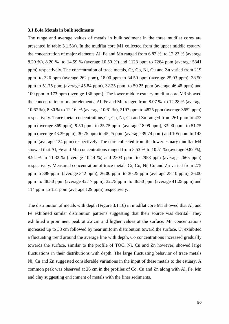
90
3.1.B.4a Metals in bulk sediments
The range and average values of metals in bulk sediment in the three mudflat cores are
presented in table 3.1.5(a). In the mudflat core M1 collected from the upper middle estuary,
the concentration of major elements Al, Fe and Mn ranged from 6.82 % to 12.23 % (average
8.20 %), 8.20 % to 14.59 % (average 10.50 %) and 1123 ppm to 7264 ppm (average 5341
ppm) respectively. The concentration of trace metals, Cr, Co, Ni, Cu and Zn varied from 219
ppm to 326 ppm (average 262 ppm), 18.00 ppm to 34.50 ppm (average 25.93 ppm), 38.50
ppm to 51.75 ppm (average 45.84 ppm), 32.25 ppm to 50.25 ppm (average 46.48 ppm) and
109 ppm to 173 ppm (average 136 ppm). The lower middle estuary mudflat core M3 showed
the concentration of major elements, Al, Fe and Mn ranged from 8.07 % to 12.28 % (average
10.67 %), 8.30 % to 12.16 % (average 10.61 %), 2197 ppm to 4875 ppm (average 3652 ppm)
respectively. Trace metal concentrations Cr, Co, Ni, Cu and Zn ranged from 261 ppm to 473
ppm (average 369 ppm), 9.50 ppm to 25.75 ppm (average 18.99 ppm), 33.00 ppm to 51.75
ppm (average 43.39 ppm), 30.75 ppm to 45.25 ppm (average 39.74 ppm) and 105 ppm to 142
ppm (average 124 ppm) respectively. The core collected from the lower estuary mudflat M4
showed that Al, Fe and Mn concentrations ranged from 8.53 % to 10.51 % (average 9.82 %),
8.94 % to 11.32 % (average 10.44 %) and 2203 ppm to 2958 ppm (average 2665 ppm)
respectively. Measured concentration of trace metals Cr, Co, Ni, Cu and Zn varied from 275
ppm to 388 ppm (average 342 ppm), 26.00 ppm to 30.25 ppm (average 28.10 ppm), 36.00
ppm to 48.50 ppm (average 42.17 ppm), 32.75 ppm to 46.50 ppm (average 41.25 ppm) and
114 ppm to 151 ppm (average 129 ppm) respectively.
The distribution of metals with depth (Figure 3.1.16) in mudflat core M1 showed that Al, and
Fe exhibited similar distribution patterns suggesting that their source was detrital. They
exhibited a prominent peak at 26 cm and higher values at the surface. Mn concentrations
increased up to 38 cm followed by near uniform distribution toward the surface. Cr exhibited
a fluctuating trend around the average line with depth. Co concentrations increased gradually
towards the surface, similar to the profile of TOC. Ni, Cu and Zn however, showed large
fluctuations in their distributions with depth. The large fluctuating behavior of trace metals
Ni, Cu and Zn suggested considerable variations in the input of these metals to the estuary. A
common peak was observed at 26 cm in the profiles of Co, Cu and Zn along with Al, Fe, Mn
and clay suggesting enrichment of metals with the finer sediments.

91
Table 3.1.5: Range and average values of metals in bulk sediments (a) and clay fraction (b) in mudflat sediments of M1, M3 and M4 of the Zuari
estuary.
M1 M3 M4
Average Range Average Range Average Range
(a) Metals in
bulk
sediments
Al % 8.2 6.82-12.23 10.67 8.07-12.28 9.82 8.53-10.51
Fe % 10.5 8.20-14.59 10.61 8.30-12.16 10.44 8.94-11.32
Mn (ppm) 5341 1123-7264 3652 2197-4876 2665 2203-2958
Cr (ppm) 262 219-326 369 261-473 342 275-388
Co(ppm) 25.93 18.00-34.50 18.99 9.50-25.75 28.1 26.00-30.25
Ni (ppm) 45.84 38.50-51.75 43.39 33.00-51.75 42.17 36.00-48.50
Cu (ppm) 46.48 32.25-50.25 39.74 30.75-45.25 41.25 32.75-46.50
Zn(ppm) 136 109-173 124 105-142 129 114-150
(b) Metals in
the clay
fraction
Al (%) 11.05 9.86-12.53 11.19 9.26-14.52 2.76 0.42-7.95
Fe (%) 7.75 6.83-8.51 7.21 6.35-8.38 2.24 0.2-7.14
Mn (ppm) 7121 6573-7618 4862 3771-5966 1699 777-3696
Cr (ppm) 506 353-575 659 501-727 615 486-791
Co (ppm) 33.81 17.25-43.75 23.94 12.00-39.00 13.25 7.00-28.00
Ni (ppm) 105 53.00-153 153 116-189 71.25 54.75-87.75
Cu (ppm) 184 161-234 170 145-179 117 87.25-174
Zn (ppm) 691 135-1064 757 428-1166 515 42.25-1717
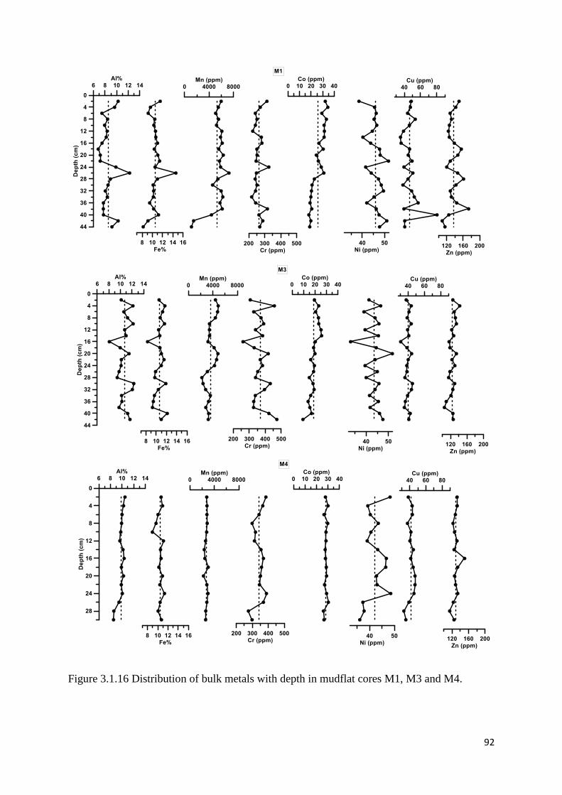
92
Figure 3.1.16 Distribution of bulk metals with depth in mudflat cores M1, M3 and M4.

93
In core M3, the distribution of metals with depth revealed that major elements Al and Fe
exhibited similar distribution pattern with fluctuations and overall increase towards the
surface. Mn concentrations increased towards the surface with higher values at 20 cm. Trace
elements of Cr and Ni showed large fluctuations with depth. Co and Zn increased towards the
surface along with Mn, whereas Cu exhibited slight increase up to 14 cm followed by
constant distribution towards the surface. The distribution of metals with depth in core M4
showed that the percentage of Al exhibited minor enrichment towards the surface and higher
values between 24 cm and 14 cm depth. The profile of Fe and Mn showed uniform
distribution pattern except for a negative peak at 10 cm for Fe. Cr and Ni and to some extent
Cu and Zn displayed similar distribution trends to Al which could indicate a detrital source
for these metals. However, among them Cr and Ni showed large fluctuations.
Pearson’s correlation analysis (Table 3.1.6) carried out on the data set for each of the mudflat
cores, helped in understanding the source and geochemical associations of the metals.
Substantial spatial and temporal variations were noted from the ranges, averages and vertical
distribution profiles of the three mudflat cores. Highest concentrations of Mn, Ni, Cu and Zn
were noted in the upper middle estuary; Al, Fe and Cr in the lower middle estuary and Co in
the lower estuary. Most metals were accumulated in higher amounts in the middle estuary
than the lower estuary due to higher estuarine hydrodynamics, which increased towards the
mouth under the influence of strong waves. Metals may have been resuspended and
mobilized under high hydrodynamic conditions in the lower estuary. Shiyuan et al. (1997)
reported that there is a close relationship between the accumulation of heavy metals and the
geomorphic features of the tidal flats in the estuary.
In the core M1 collected from the upper middle estuary mudflat, metal distributions were less
influenced by sediment grain size. Fe and Mn were significantly associated indicating
similarity in their redox behaviors. Fe-Mn oxides accounted for the down-core variation of
metals Co and Zn in the sediments. Fe and Mn oxides are very effective scavengers for trace
metals and play an important role in the remobilization processes of the adsorbed trace metals
between the sediments, pore water, and overlying water (Amiard-Triquet and Rainbow,
2009). Additionally, Mn was significantly associated with the silt size particles. The
fluctuating trends of Ni, Cu and Zn suggested large variations in their inputs to the estuary
and their poor association to the lithogenic elements.

94
Table 3.1.6: Pearson’s correlation coefficient of sediment components and bulk metals in mudflat cores of M1, M3 and M4.
(a) Correlations-M1 pH Sand Silt Clay TOC Al Fe Mn Cr Co Ni Cu Zn
pH 1.00
Sand 0.58** 1.00
Silt -0.63** -0.63** 1.00
Clay 0.51* 0.33 -0.94** 1.00
TOC -0.53* -0.54** 0.540** -0.42 1.00
Al 0.11 0.27 -0.42 0.39 -0.11 1.00
N=22
Fe -0.18 -0.48* 0.19 -0.02 0.18 0.37 1.00
Mn -0.57** -0.74** 0.58** -0.38 0.32 -0.10 0.64** 1.00
Cr 0.26 0.19 -0.41 0.41 -0.22 0.29 -0.03 -0.13 1.00
Co -0.47* -0.56** 0.26 -0.07 0.61** 0.19 0.33 0.43* 0.07 1.00
Ni 0.50* 0.29 -0.09 -0.01 -0.06 -0.29 -0.22 -0.43* -0.37 -0.44* 1.00
Cu -0.12 -0.11 0.05 -0.01 -0.34 -0.08 0.21 0.05 -0.25 -0.24 0.10 1.00
Zn -0.30 -0.22 0.36 -0.34 0.12 -0.11 0.33 0.53* 0.10 0.05 -0.15 -0.03 1.00
(b) Correlation M3
pH Sand Silt Clay TOC Al Fe Mn Cr Co Ni Cu Zn
pH 1.00
Sand 0.13 1.00
Silt -0.09 0.10 1.00
Clay 0.03 -0.44* -0.94** 1.00
TOC 0.00 -0.17 -0.39 0.42 1.00
Al -0.20 0.16 -0.08 0.01 -0.34 1.00
N=21
Fe -0.37 0.25 0.13 -0.21 -0.14 0.76** 1.00
Mn -0.56** -0.23 -0.13 0.20 0.25 0.09 0.37 1.00
Cr -0.09 0.39 -0.20 0.04 -0.05 0.83** 0.73** 0.06 1.00
Co -0.54* -0.43 0.17 0.00 -0.01 0.19 0.19 0.33 -0.08 1.00
Ni 0.08 0.15 -0.27 0.19 0.05 0.71** 0.56** 0.15 0.75** -0.11 1.00
Cu -0.12 0.09 -0.02 -0.02 -0.15 0.93** 0.83** 0.18 0.80** 0.21 0.72** 1.00
Zn -0.61** 0.00 -0.10 0.09 0.08 0.70** 0.75** 0.53* 0.65** 0.50* 0.39 0.73** 1.00

95
(c ) Correlations- M4 pH Sand Silt Clay TOC Al Fe Mn Cr Co Ni Cu Zn
pH 1.00
Sand 0.66** 1.00
Silt -0.67** -0.57* 1.00
Clay 0.29 -0.09 -0.77** 1.00
TOC -0.35 -0.40 0.70** -
0.54*
1.00
Al -0.51 -0.72** 0.57* -0.13 0.32 1.00
N=15
Fe 0.35 0.13 -0.15 0.08 0.07 0.16 1.00
Mn -0.06 -0.17 0.38 -0.33 0.40 0.01 -0.21 1.00
Cr -0.17 -0.41 0.34 -0.10 0.22 0.75** 0.46 0.17 1.00
Co -0.16 -0.40 0.10 0.18 0.33 0.41 0.11 0.25 0.39 1.00
Ni -0.07 -0.33 0.35 -0.17 0.11 0.72** 0.17 0.21 0.63* 0.12 1.00
Cu -0.18 -0.39 0.39 -0.17 0.11 0.68** 0.25 -0.01 0.62* 0.22 0.45 1.00 Zn -0.08 -0.62* 0.31 0.11 0.18 0.60* 0.37 0.02 0.61* 0.13 0.58* 0.40 1.00

96
Metals in the intertidal sediments may partially originate from the weathering of parent rocks,
may also stem from wastewater discharges or atmospheric deposition and are mostly retained
or adsorbed by intertidal sediments of the estuary (Xue-Feng et al., 2013). Al, Fe and Mn
indicated they are of mixed origins probably anthropogenic. Co however, showed association
with TOC which implied that Co might have been mobilized through processes involving
organic materials. The increasing distribution pattern of Co suggested recent inputs and a
different source from other trace metals. The concentrations of Cr, Co, Ni, Cu and Zn along
with Al above 14 cm, increased towards the surface implying detrital input of these metals in
the recent past. Thus, in the upper estuarine mudflat, metal distributions were influenced by
Fe and Mn and were anthropogenic in nature.
In the core M3 collected from the lower middle estuary, the influence of sediment
components on metal distributions was noted to be negligible. Modification of sediments
with respect to early diagenetic changes in reductive dissolution of Fe and Mn was very
prominent between 22 cm to 20 cm. Under the sediment–water interface, the reductive
dissolution of Mn and Fe oxides leads to the remobilization of initially bound trace elements
which further can be re-adsorbed onto or co-precipitated with newly-formed Mn and Fe
mineral phases (Dang et al., 2015). Cr, Ni, Cu and Zn were associated with Al and Fe. As, Al
is a naturally occurring metal and its concentration is generally not influenced by
anthropogenic sources (Schropp and Windom, 1988), metal associations with Al suggested a
detrital source influencing metal distributions. Metal distribution patterns also exhibited
constant or decreasing trends towards the surface, which suggested reduced anthropogenic
inputs. Co, in a similar manner to the upper middle estuary, increased towards the surface.
Thus a common source of Co may have influenced the upper middle and lower middle
estuary.
The sediments of core M4 collected from the lower estuary showed little variations in the
distribution pattern of metals. Metal distributions were less affected by sediment components.
Association of metals Cr, Ni, Cu and Zn with Al and their significant inter-metal association
suggested a detrital source. The uniform distribution of most metals suggested a constant rate
of input of metals. Overall, metal distributions in this core were influenced by
aluminosilicates.

97
On comparing the distribution profile of metals with clay minerals, no significant association
was evident. This indicated that the clay mineralogy had very little influence on metal
distribution and was more influenced by other sediment components and physiochemical
processes. The major clay minerals of illite, kaolinite as well as chlorite weakly associated
with all the investigated trace metals probably due to the weak competing strength of these
clays compared with the other adsorbents and to low availability of the mobile trace metals in
the system (He et al., 2012).
Additionally, an attempt was made to understand that association of metals with the magnetic
material in the sediments by comparing distribution profiles. In mudflat core M1, the Cr
profile showed similarity with χARM that implied that some amount of Cr might have been
anthropogenically sourced to the upper middle estuary sediments. Association of Mn and Co
with the magnetic grain size parameters suggests their association with the fine grains.
Scraps containing rust fragments and paints enriched in heavy metals may have settled
through the water column and eventually deposited in the sediments and caused high levels of
magnetic susceptibility. No significant association of metals with the magnetic susceptibility
parameters were noted in core M3, that suggested that this region of the estuary subjected to
low amount of the pollutant load as compared to other regions of the estuary. In core M4, Cr
and Ni showed similar distribution to SIRM suggesting that Cr and Ni may be associated
with some amount of ferromagnetic materials as SIRM primarily responds to the
concentration of ferrimagnetic material in the sediments such as magnetite.
Magnetic particles in the sediments may be detrital derived geologically from catchment area
sources; anthropogenic, if they are derived from industrial emissions and atmospheric; or
biogenic in nature. The strong similarity in distribution between magnetic susceptibility and
several sediment metal concentrations suggested a significant contribution to the magnetic
material from anthropogenic sources (Chan et al., 1998). The ferric oxide and trace metals are
associated as metals are preferentially adsorbed on to the exterior surface of Fe- oxides and
precipitated to the sediments. Thus, the metals associated with the magnetic material may
have been supplied anthropogenically from mining and shipbuilding discharges.
3.1. B.4b Metals in the clay fraction of sediments
Further, the geochemistry of the clay fraction of sediments was studied as metals have a
strong tendency to associate with the fine sediments. The range and average values of metals

98
content in the clay fraction of cores M1, M3 and M4 are presented in Table 3.1.5(b). In the
mudflat core M1, concentrations of major elements Al, Fe and Mn ranged from 9.86 % to
12.53 % (average 11.05 %), 6.83 % to 8.51 % (average 7.75 %) and 6573 ppm to 7618 ppm
(average 7121 ppm). Trace metal concentrations of Cr, Co, Ni, Cu and Zn in the core ranged
from 353 ppm to 575 ppm (average 506 ppm), 17.25 ppm to 43.75 ppm (average 33.81
ppm), 53.00 ppm to 153 ppm (average 105 ppm), 161 ppm to 234 ppm (average 184 ppm)
and 135 ppm to 1064 ppm (average 691 ppm). The concentrations of major elements Al, Fe
and Mn in the sediment core M3 collected from the lower middle estuary mudflat ranged
from 9.26 % to 14.52 % (average 11.19 %), 6.35 % to 8.38 % (average 7.21 %) and 3771
ppm to 5966 ppm (average 4862 ppm ) respectively. Further, the trace metal concentrations
of Cr, Co, Ni, Cu and Zn ranged from 501 ppm to 727 ppm (average 659 ppm), 12.00 ppm to
39.00 ppm (average 23.94 ppm), 116 ppm to 189 ppm (average 153 ppm), 145 ppm to 179
ppm (average 170 ppm) and 428 ppm to 1166 ppm (average 757 ppm) respectively. In
sediment core M4 collected from the lower estuary mudflat, major elements Al, Fe and Mn
concentrations ranged from 0.42 % to 7.95 % (average 2.76 %), 0.20 % to 7.14 % (average
2.24 %) and 777 ppm to 3696 ppm (average 1699 ppm) respectively. Trace metals Cr, Co,
Ni, Cu and Zn concentrations ranged from 486 ppm to 791 ppm (average 615 ppm ), 7.00
ppm to 28.00 ppm (average 13.25 ppm), 54.75 ppm to 87.75 ppm (average 71.25 ppm), 87.25
ppm to 174 ppm (average 117 ppm) and 42.25 ppm to 1717 ppm (average 515 ppm).
Highest average concentration of Fe, Mn, Co and Cu was noted in the upper middle estuary
mudflat, Al, Cr, Ni and Zn in the lower middle estuary mudflat and the lowest concentration
of most trace metals in the clay fraction (except for Cr) was noted in the lower estuary.
From the vertical distribution of metals in the clay fractions (Figure 3.1.17) in core M1, it
was observed that Al and Fe showed similar distribution trends wherein concentrations
increased up to 30 cm followed by a minor decrease towards the surface. The trace metals Cr,
Co, Ni, Cu and Zn exhibited similar distribution pattern among themselves and to the profiles
of Al and Fe suggesting their common source that was mainly detrital. Mn concentrations
showed a minor increase up to 14 cm followed by decrease towards the surface and exhibited
a distribution pattern different from Al and Fe suggesting some alternative source possibly
anthropogenic.

99
Figure 3.1.17 Distribution of metals in the clay fraction of sediments with depth in mudflat
cores M1, M3 and M4.
In the vertical distribution of metals in the clay fraction of sediments of mudflat core M3, Al
distribution exhibited a peak at 30 cm followed by decrease up to 22 cm and then constant

100
values towards the surface. Fe concentrations decreased up to 30 cm and showed near
uniform distribution towards the surface. Mn concentrations gradually increased towards the
surface with a prominent peak at 6 cm. The trace metals exhibited distinct distribution
patterns wherein Cr gradually increased towards the surface along with Mn, while, Co
exhibited a fluctuating distribution with peaks at 14 cm and 6 cm that corresponded to Mn.
Ni, Cu and Zn exhibited similar distributions along with Al below 18 cm, followed by
distinct distribution towards the surface that corresponded to Mn. From the vertical profile of
metals in the clay fraction of mudflat core M4 showed that Al, Fe and Mn exhibited a
corresponding distribution pattern with a prominent peak at 18 cm. Similar peak was noted in
the profiles of Cr, Co and Cu. The concentrations of Co above 10 cm and Ni above 18 cm
were below detection limits. Zn however, exhibited a peak in its distribution profile at 10 cm
followed by low concentrations at the surface suggesting a difference source.
The comparison of metal profiles in clay fraction (Table 3.1.5) of core M1 revealed that all
metals were associated with Al and Fe, which indicated the role of aluminosilicates and Fe-
oxyhydroxides in the distribution of the trace metals. The trace metals however, were weakly
associated with Mn. Similar distributions of Cr, Co, Ni and Zn suggested a common source
for these metals. In core M3, all metals in the clay fraction were associated with Mn
suggesting the role of Mn-oxyhydroxides in the distribution of the trace metals. Similar
distributions of Ni and Cu indicated a common source for these two metals. Similar
distributions of Al, Fe and Mn along with the trace metals in sediment core M4 suggested the
terrigenous origin of these metals.
Further, comparison of average metal concentrations in the bulk sediments and clay fraction
using the isocon diagram (Figure 3.1.18) was established. In the upper middle and lower
middle estuary, concentrations of all metals except for Fe were high in the clay fraction
indicating a detrital control for Al, Mn, Cr, Co, Ni, Cu and Zn and were mainly associated
with aluminosilicates. Zn, Ni and Cu however, formed a group of high concentrations in the
clay fraction. Further, Fe may have been associated with larger sediment particles or may
have formed larger aggregates of iron oxides. In the lower estuary mudflat core M4, Cr, Ni,
Cu and Zn concentrations were high in the clay fraction of sediments whereas Al, Fe, Mn and
Co concentrations were higher in the bulk sediments. The association of Al, Fe and Mn with
the coarse sediments suggested physically weathered coarse material or deposition of ore
material in the sediments that may have come from the spillage from ore carrying barges.

101
Figure 3.1.18: Isocon diagram of metals in bulk sediments versus metals in the clay fraction
of mudflat cores M1, M3 and M4.
Metals are known to be more adsorbed to the smaller sediment particles especially clay than
the coarser fractions. Higher concentrations of metals found in the finer sediment particles are
due to the synergetic action of physical and chemical properties of the particles of each size
fraction. The smaller sediment grains have a greater specific surface area than the larger
grains. Also, most fine particles consist mainly of clay minerals, which have more metal
binding sites than the silicate or carbonate minerals, which are the major components of
coarser material in marine sediments (Campbell et al., 1988).
In general, the coarse material is an important constituent of the sediment and may represent
more than 50 percent of the bulk sediment mass. Although high metal concentrations can be
occasionally found in coarse sediment material (Filipek et al., 1981; Robinson, 1982), the silt
and clay fractions usually contain higher metal concentrations than the sand fraction. The
vicinity of land based pollution sources, which may dispose large particles with relatively
high metal content through urban and industrial effluents and deposits, may lead to enhanced
metal concentrations in coarse sediment material (Horowitz, 1991). Metal enrichments in

102
coarse sediments may be explained by the formation of coatings on the surface of the
particles (Krumgalz et al., 1992) through carbonates, hydroxy-oxides and organic matter that
enhance the specific surface area of particles that may lead to the increase of their adsorption
capacity (Horowitz and Elrick, 1987). The coating formation may also bring about the
consolidation of fine particles to the formation of larger particles with smaller specific
surface area and thus, smaller adsorption capacity. The particle consolidation may also lead
to an ‘artificial’ enhancement of metal concentrations in the coarser sediment fractions
(Aloupi and Angelidis, 2002). Thus, most Fe may have been of anthropogenic origin and the
associated metals like Mn, Co in the lower estuary may have led to the formation of coating
around the larger sediment grains.
3.1.C Comparison of mangrove and mudflat core sediments in the Zuari estuary
Figure 3.1.19: Isocon diagram of metals in mudflat sediments versus mangrove of sediments
collected from Station 1 of the upper middle estuary, station 3 of the lower middle estuary
and station 4 of the lower estuary.
A comparison of sediment components and metals in the mangrove cores with the mudflat
cores collected at the sampling locations 1, 3 and 4 using the isocon diagram was made to
understand the degree of metal association within each of the estuarine sub-environments and
the processes controlling them.
103
In the upper middle estuary (station 1), the average values plotted on the isocon diagram
(Figure 3.1.19) revealed higher content of sand, silt, Mn, Co, Ni and Cu in the mudflat
whereas clay, TOC , Cr and Zn were higher in the mangrove. In the lower middle estuary
(station 3), sand, clay, Mn and Cr were high in the mudflat whereas silt, Co, Ni, Cu and Zn
were higher in the mangrove. In the lower estuary (station 4), silt, clay, TOC, Al, Fe, Mn, Co,
Cu, Ni and Zn were higher in the mudflat sediments whereas sand was higher in the
mangrove.
The sediments of the upper middle estuary showed less variation with respect to the sediment
components and metal concentrations as most of the point fell close to the central line.
Proceeding seawards, the variation in the sediment component and metals increased and with
highest variation observed in the lower estuary. This difference was mainly due the
geomorphic characteristics and the physical processes in the estuary. The Mormugao Bay, at
the mouth of the Zuari River, is relatively large in area and is funnel-shaped with a width of 5
km at the mouth and narrows down to 1 km at the joining point of the channel. The funnel-
shaped bay favors the enhancement of physical processes. Sampling location 1 was located in
close proximity to the upstream region of the estuary where much of the fluvial sedimentary
material is supplied. The narrow width of the canal and the less magnitude of the tidal
currents in the upstream regions of the estuary facilitated quick removal of material from the
water column to the sediments. Thus, less variation between the mudflats and mangrove
sediment components were observed. In the mudflat, higher content of Co, Ni and Cu may be
probably associated with the Fe-Mn oxyhydroxides whereas enrichment of Cr and Zn in the
mangrove may be associated with Fe oxides and TOC. The mangrove sediments contain
higher percentage of organic matter that may be related to the accumulation of litter within
the mangrove forest (Tam and Wong, 1998). In the lower middle estuary, the relatively
broader width of the channel allowed for an increased tidal magnitude and thus may have
caused resuspension of sediments to the water column which facilitated sorting of material
and its subsequent deposition in the intertidal regions. Higher Cr content in the mudflats may
have been influenced by sand, clay, Mn-oxides whereas Co, Ni, Cu and Zn in mangroves
were positively correlated with silt and thus co-precipitated together. In the lower estuary, the
broad width of the bay and the high energy conditions caused turbulence due to which much
of the sediments were re-suspended and transported to calmer regions. The larger grain size
material got trapped in the mangroves due to the effect of the specialized network of

104
mangrove roots called pneumatophores that aid in trapping larger grain size particles brought
in by the tide. The fine sediments along with adsorbed metals accumulated in the mudflats.
Additionally the coarse calcareous material in the mangrove sediments provides little surface
for adsorption of metals. The accumulation of Co, Cu, Ni and Zn in mudflats is attributed to
the higher silt, clay, TOC, Al, Fe, Mn that facilitated the accumulation of metals. In the lower
estuary, metals in the mudflat are associated with silt and clay particles due to the processes
of adsorption and coagulation (Anithamary et al., 2012).
The transfer and the chemical stability of metal contaminants in sediments are controlled by a
complex series of biogeochemical processes depending on parameters like pH, clay content,
and redox potential (Vanbroekhoven et al., 2006). Mangroves are known for the high organic
matter content and their sediments are favorable to reducing conditions, where metals can be
immobilized in the form of sulfides or complexed with organic matter (da Silva et al., 2014).
Oxidizing conditions generally increase the retention capacity of metals in sediments, while
reducing conditions will generally lessen the retention capacity of metals (McLean and.
Bledsoe, 1992). The decomposition of the organic matter received in the mangroves provides
reducing conditions in the mangroves that causes mobility of redox sensitive elements Fe and
Mn along with associated metals. These mobilized metals may either get re-precipitated at the
oxidizing surface of the sedimentary column or may escape to the water column. This was
evident from the marginally higher TOC content in mangroves from the isocon diagram. The
mudflat habitat provides an interesting case study in metal geochemistry in a system with a
high suspended particulate concentration through ebb and flood tide (Rezaie-Boroon et al.,
2013). During the transition to oxidizing condition in ebb, solid iron oxide (e.g. FeOOH) will
precipitate dramatically, reducing the mobility of metals, which co-precipitate with iron
(Andrews et al., 2004). Thus, the mobilized metals from the mangrove sediments are trapped
along with oxides of Fe and Mn in the mudflat sediments, which was evident from the higher
Mn content in the mudflat sediments along with metals.
3.1.D Enrichment Factor and Geoaccumulation index
Enrichment factors and Geoaccumulation index were calculated to assess the extent of metal
enrichment and pollution levels of the estuary. The average values of the enrichment factors
are present in table 3.1.7 for mangroves and mudflats at each of the sampling locations.
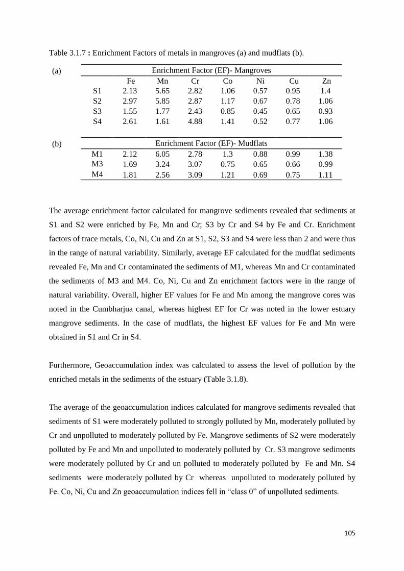
105
Table 3.1.7 : Enrichment Factors of metals in mangroves (a) and mudflats (b).
(a) Enrichment Factor (EF)- Mangroves
Fe Mn Cr Co Ni Cu Zn
S1 2.13 5.65 2.82 1.06 0.57 0.95 1.4
S2 2.97 5.85 2.87 1.17 0.67 0.78 1.06
S3 1.55 1.77 2.43 0.85 0.45 0.65 0.93
S4 2.61 1.61 4.88 1.41 0.52 0.77 1.06
(b) Enrichment Factor (EF)- Mudflats
M1 2.12 6.05 2.78 1.3 0.88 0.99 1.38
M3 1.69 3.24 3.07 0.75 0.65 0.66 0.99
M4 1.81 2.56 3.09 1.21 0.69 0.75 1.11
The average enrichment factor calculated for mangrove sediments revealed that sediments at
S1 and S2 were enriched by Fe, Mn and Cr; S3 by Cr and S4 by Fe and Cr. Enrichment
factors of trace metals, Co, Ni, Cu and Zn at S1, S2, S3 and S4 were less than 2 and were thus
in the range of natural variability. Similarly, average EF calculated for the mudflat sediments
revealed Fe, Mn and Cr contaminated the sediments of M1, whereas Mn and Cr contaminated
the sediments of M3 and M4. Co, Ni, Cu and Zn enrichment factors were in the range of
natural variability. Overall, higher EF values for Fe and Mn among the mangrove cores was
noted in the Cumbharjua canal, whereas highest EF for Cr was noted in the lower estuary
mangrove sediments. In the case of mudflats, the highest EF values for Fe and Mn were
obtained in S1 and Cr in S4.
Furthermore, Geoaccumulation index was calculated to assess the level of pollution by the
enriched metals in the sediments of the estuary (Table 3.1.8).
The average of the geoaccumulation indices calculated for mangrove sediments revealed that
sediments of S1 were moderately polluted to strongly polluted by Mn, moderately polluted by
Cr and unpolluted to moderately polluted by Fe. Mangrove sediments of S2 were moderately
polluted by Fe and Mn and unpolluted to moderately polluted by Cr. S3 mangrove sediments
were moderately polluted by Cr and un polluted to moderately polluted by Fe and Mn. S4
sediments were moderately polluted by Cr whereas unpolluted to moderately polluted by
Fe. Co, Ni, Cu and Zn geoaccumulation indices fell in “class 0” of unpolluted sediments.

106
Table 3.1.8 : Geoaccumulation index of metals in mangroves (a) and mudflats (b).
(a) Geoaccumulation index (Igeo)-Mangroves
Fe Mn Cr Co Ni Cu Zn
S1 0.61 2.01 1 -0.42 -0.85 -0.57 0
S2 1.02 1.9 0.97 -0.33 -0.69 -0.91 -0.47
S3 0.57 0.68 1.22 -0.31 -0.76 -0.69 -0.17
S4 0.36 -0.36 1.27 -0.69 -1.49 -1.37 -0.9
(b) Geoaccumulation index (Igeo)-Mudflats
M1 0.56 1.97 0.95 -0.17 -0.71 -0.56 -0.07
M3 0.58 1.48 1.44 -0.62 -0.8 -0.77 -0.2
M4 0.56 1.06 1.33 -0.02 -0.84 -0.72 -0.15
Geoaccumulation index was also calculated for the metals of the mudflats sediments.
According to the established classification of the geoaccumulation index, sediments of
mudflat core S1 were moderately polluted by Mn and unpolluted to moderately polluted by
Fe and Cr. In the mudflat sediments of core S3 and S4, Mn and Cr were moderately polluted
and unpolluted to moderately polluted by Fe. The sediment at all three mudflat location fell in
“class 0” of unpolluted sediments for Co, Ni, Cu and Zn.
Overall, similar to EF in the mangroves highest Igeo values of Fe were noted in S2, Mn in S1
and Cr in S4. In the case of mudflats, highest Igeo value for Fe was noted in M3, Mn in M1
and Cr in M3. The lowest EF and Igeo was noted for Ni in the mangroves as well as
mudflats.
Thus, average EF values and geoaccumulation indices of Fe, Mn and Cr indicated significant
anthropogenic inputs of Fe, Mn and Cr in to the estuary. Co, Ni, Cu and Zn did not show
enrichment in the estuarine sediments and are of natural origin.
The Zuari estuary receives a large input of mining material from Mandovi estuary via the
Cumbharjua canal. Part of this material must have settled within the canal leading to the
enrichment of Fe, Mn and Cr in the sediments. The enrichment of Fe and Mn in core S1 and
Mn in core S1 was probably salinity dependent in addition to mining input. Fe and Mn is
supplied to the riverine flow in reduced and soluble Fe(II) and Mn (II) state which undergoes
oxidative conversion to insoluble Fe (III) and Mn (IV) state as the riverine waters encounter

107
saline waters (Chester and Jickells, 2012). The behavior of Fe and Mn is similar but Fe is
precipitated at lower salinities compared to Mn. Dessai and Nayak (2009) noted that higher
salinity of the waters was maintained from the mouth of the Zuari estuary up to slightly
upstream of the Cumbharjua canal. Thus, in the upper middle estuary, much of the Fe and Mn
were removed from the solution to the sediments on encountering waters of higher salinity.
Cr, however, showed higher Igeo values in the lower estuary that decreased towards the
upper middle estuary. Association of Cr with Fe ores was earlier reported (Bukhari, 1994)
within the catchment of the Mandovi estuary that is connected to the Zuari estuary via the
Cumbharjua canal. Ore processing units operate all along the banks of the estuary and these
industries release associated elements to the waters of the estuary. In addition, the loading
jetties in the upstream of Zuari estuary are also expected to release considerable amount of
Fe, Mn and Cr. Cr may have been released as leachates from loading of mining ores and
shipping activities at the Mormugao harbor located nearby and may have accumulated in the
sediments. Additionally, Cr may be released from effluents from treated domestic sewage and
industrial discharges and corrosion of uncoated steels from ships in the harbor at the mouth
and ship building industries located along the estuary.
3.1.E Speciation of metals (Fe, Mn, Cr, Co, Cu and Zn)
The sequential extraction of metals within the five geochemical phases viz. exchangeable
(F1), carbonate (F2), Fe-Mn oxide (Reducible- F3), organic matter/sulfide bound
(Oxidisable- F4) and residual (F5) was estimated for selected sub-samples of the cores of the
mangroves and mudflats of the Zuari estuary. The non-residual metals (F1 to F4) are
considered to represent the bioavailable fraction of total metal content of the sediments
(Loring and Hill, 1992).
3.1.E.1 Mangroves
The average values of metals in the five geochemical fractions are presented in table 3.1.9
and their respective ranges are described below.

108
Table 3.1.9: Average values of metals in the five sedimentary fractions of the mangrove sediments and their respective % in parenthesis.
Exchangeable Carbonate Fe-Mn oxide Organic/Sulfide Residual
(ppm) (%) (ppm) (%) (ppm) (%) (ppm) (%) (ppm) (%)
Fe S1 11.76 0.01 5.80 0.01 8129 9.54 1272 1.48 76319 88.96
S2 13.34 0.01 8.95 0.01 7131 6.98 1246 1.23 95834 91.76
S3 50.12 0.06 6.98 0.01 5144 6.45 1707 2.26 72791 91.22
S4 64.62 0.01 28.5 0.04 3694 5.57 156 0.24 62849 94.05
Mn S1 600 11.10 1982 36.23 2165 39.55 246 4.48 469 8.64
S2 756 13.24 786 14.28 3500 56.36 286 4.76 628 11.36
S3 484 21.76 487 19.70 698 28.39 195 8.07 508 22.08
S4 83.85 5.45 263 18.32 348 28.79 150 11.18 418 35.63
Cr S1 1.38 0.64 0.91 0.43 11.53 5.39 12.92 6.05 189 87.50
S2 0.90 0.47 1.34 0.70 9.87 5.10 11.24 5.84 171 87.89
S3 2.22 1.02 1.05 0.48 12.87 5.92 24.88 11.36 178 81.22
S4 1.17 0.55 1.75 0.82 11.33 5.37 10.79 5.21 187 88.05
Co S1 1.16 2.42 1.08 2.23 9.36 19.73 3.13 6.62 33.15 69.00
S2 1.04 2.63 1.00 2.25 10.82 27.67 2.28 5.88 24.20 61.27
S3 2.11 4.62 1.32 2.87 5.94 12.97 2.65 5.78 33.80 73.76
S4 1.63 4.74 2.41 7.12 4.66 13.59 0.98 2.74 24.98 71.81
Cu S1 1.26 1.30 1.56 1.60 2.74 2.79 22.25 22.10 73.79 71.21
S2 1.35 1.46 1.13 1.23 2.17 2.35 11.18 12.27 85.23 82.68
S3 0.89 1.22 0.87 1.18 1.37 1.83 12.46 16.64 59.02 79.13
S4 1.09 2.42 1.29 3.18 0.63 1.40 3.58 7.63 37.87 85.36
Zn S1 0.61 0.56 1.64 1.48 21.26 19.32 9.69 8.89 76.72 69.73
S2 0.75 0.92 1.37 1.68 12.73 15.40 6.07 7.49 61.42 74.50
S3 1.21 1.19 1.69 1.56 13.33 12.48 6.67 6.57 84.64 78.20
S4 3.99 5.09 1.63 2.66 10.58 15.34 2.34 3.41 49.72 73.49

109
3.1.E.1a Iron
In mangrove core S1, Fe association with different fractions varied in the order of abundance
F5>F3>F4>F1>F2. The concentration of Fe in the residual phase (F5) varied from 67198
ppm to 86623 ppm (average 76319 ppm) that accounted for 85 % to 91 % (average 88.96 %)
when recalculated taking all the five fractions to hundred percent. Following residual, Fe was
enriched in the Fe-Mn oxide bound fraction ranging from 6723 ppm to 9053 ppm (average
8129 ppm) that accounted for 7.27 % to 11.07 % (average 9.54 %). Fe in the organic/ sulfide
bound fraction varied from 640 ppm to 2820 ppm (average 1272 ppm) that accounted for
0.67 % to 3.05 % (average 1.48 %) while, Fe in the exchangeable phase ranged from 0.30
ppm to 44.03 ppm (average 11.76 ppm) that accounted for 0.0003 % to 0.05 % (average 0.01
%). The lowest concentrations of Fe were associated with the carbonate phase that ranged
from 1.00 ppm to 15.80 ppm (average 5.80 ppm) that accounted for 0.001 % to 0.019 %
(average 0.007 %). The concentration of Fe in core S2 in different sediment fractions varied
in the order of abundant F5>F3>F4>F1>F2. The concentration of Fe in the residual phase
(F5) varied from 78963 ppm to 112773 ppm (average 95834 ppm) that accounted for 89 % to
95 % (average 91.76 %) when recalculated taking all five fractions to hundred percent.
Following residual, Fe was enriched in the Fe-Mn oxide bound fraction ranging from 4685
ppm to 9368 ppm (average 7131 ppm) that accounted for 3.95 % to 9.21 % (average 6.98 %).
Fe in the organic/ sulfide bound fraction varied from 734 ppm to 1725 ppm (average 1246
ppm) that accounted for 0.64 % to 2.00 % (average 1.23 %) while, Fe in the exchangeable
phase ranged from 0.43 ppm to 55.25 ppm (average 13.34 ppm) that accounted for 0.0004 %
to 0.05 % (average 0.013 %). The lowest concentrations of Fe were noted in the carbonate
phase that ranged from 0.30 ppm to 60.58 ppm (average 8.95 ppm) that accounted for 0.0003
% to 0.07 % (average 0.0097 %). In core S3, the distribution of Fe was in the order of
abundance F5> F3> F4>F1> F2. Fe in the residual fraction varied from 59323 ppm to 84468
ppm (average 72790 ppm) that accounted for 84 % to 94 % (average 91.22 %) when
recalculated taking all five fractions to hundred percent. Fe in the Fe- Mn oxide bound
fraction varied from 3803 ppm to 6375 ppm (average 5144 ppm) that accounted to 4.99 % to
7.66 % (average 6.45 %) while, Fe concentrations in the organic/ sulfide fraction ranged from
582.5 ppm to 5653.55 ppm (average 1707 ppm) that accounted for 0.64 % to 8.03 % (average
2.26 %). Less quantity of Fe was associated with the exchangeable fraction ranging from
26.40 ppm to 100.30 ppm (average 50.12 ppm) that accounted to 0.04 % to 0.12 % (average
0.06 %). The lowest concentration of Fe was in the carbonate bound fraction ranging from

110
0.525 ppm to 31.175 ppm (average 6.98 ppm) that accounted to 0.0005 % to 0.03 % (average
0.01 %). The concentration of Fe in core S4, varied in the order of abundance F5> F3>
F4>F1> F2. Fe in the residual fraction varied from 55893 ppm to 70325 ppm (average 62849
ppm) that accounted for 92 % to 96 % (average 94.05 %) when recalculated taking all five
fractions to hundred percent. Fe in the Fe- Mn oxide bound fraction varied from 3033 ppm to
4403 ppm (average 3694 ppm) that accounted to 4.12 % to 6.96 % (average 5.57 %) while,
Fe concentrations in the organic/ sulfide fraction ranged from 61.73 ppm to 228 ppm
(average 155.81 ppm) that accounted for 0.08 % to 0.35 % (average 0.24 %). Some amount
of Fe was associated with the exchangeable fraction ranging from 26.70 ppm to 147.85 ppm
(average 64.62 ppm) that accounted to 0.04 % to 0.23 % (average 0.10 %). The lowest
concentration of Fe was noted in the carbonate bound fraction ranging from 1.40 ppm to
143.85 ppm (average 28.50 ppm) that accounted to 0.002 % to 0.23 % (average 0.04 %).
Overall, Fe followed the same order of abundance F5>F3>F4>F1>F2 in the four mangrove
cores. Further Fe in the residual phase varied from 88.96 % to 94.05 %, highest being in core
S4. Fe in the Fe-Mn oxide phase ranged from 5.57 % to 9.54 %, highest being in core S1. Fe
in the organic/ sulfide fraction varied from 0.24 % to 2.26 % highest being in core S3.
Fractions F1 and F2 in all the cores were less than 1 %.
Figure 3.1.20 Speciation of Fe in cores S1, S2, S3 and S4.

111
From the distribution of Fe with depth in the five sediment fractions of core S1 (Figure
3.1.20) Fe in the residual fraction was highest at all depths. Next to residual, Fe was enriched
in the Fe-Mn-oxide phase with highest concentrations at 14 cm. The concentration of Fe in
the organic/sulfide bound phase was significant at depth 30 cm and 14 cm which suggested
the formation of iron sulfides. In the distribution of Fe with depth in the five phases of core
S2, the residual fraction of Fe was the dominant sedimentary fraction with depth. The
concentration of Fe in the Fe-Mn oxide fraction was relatively low at depths below 14 cm.
followed by higher concentrations towards the surface. Significant concentration of Fe in
organic/sulfide phase was noted at depths at 40, 6 and 4 cm. The distribution of Fe with depth
of core S3 showed that highest concentration was associated with the residual phase. The
concentration of residual Fe at depths 40 cm and 30 cm were slightly lower than those depths
towards the surface. The concentration of Fe in the Fe-Mn oxide phase did not exhibit large
variations with depth. The organic/ sulfide bound Fe was higher in concentration at depth 40
cm, 30 cm and 8 cm indicating the presence of iron sulfides. Fe in the exchangeable and
carbonate fraction was found to be negligible. In core S4, the distribution of Fe with depth in
the different phases showed that the dominant fraction of Fe was the residual phase
throughout the core. Fe in the Fe- Mn fraction exhibited increased concentrations towards the
surface. Fe in fractions F4, F1 and F2 was in traces.
The data obtained showed that Fe maintained over 90 % in residual fraction, in all the four
cores with depth. Iron in the residual fraction is immobile and not available to organisms as it
is bound to primary and secondary minerals (Tessier et al., 1979). Highest average
concentration of Fe in the Fe-Mn oxide bound fraction was noted in core S1 due to
precipitation of Fe at low salinities whereas highest average concentration of Fe in the
exchangeable and carbonate fractions was noted in the lower estuary. Analysis of magnetic
parameters (S-ratio) indicated that high coercivity minerals such as haematite like minerals
phases were dominating in the upper estuarine region and less haematite like minerals are
dominating in the lower estuarine region. Dessai et al. (2009) studied the magnetic
susceptibility of the surface sediments of the Zuari estuary and noted soft (magnetite like
phase) and hard (haematite like phase) minerals are contributing to the sediment. The iron ore
deposits of Goa are essentially of hematite and are associated with ferrogenous quartzite and
phylites. The iron ore mined in the hinterland is transported and stored on the riverbanks in
the upstream region. Winds and rains erode these stacks of ores into the river, carrying along
with it the sediments in suspension. These suspended sediments were deposited in the estuary

112
causing elevated concentrations of Fe. Singh et al. (2014) found an increase in organic carbon
and ferromagnetic minerals together with high sand content that suggested the possibility of
more terrigenous input, which was reflected through increase in sedimentation rate.
Veerasingam et al. (2015) also found polyhedral iron oxide particles in the sediments that are
coarse grained iron particles of lithogenic origin derived from natural weathering processes.
The transport of material from the Mandovi estuary to the Zuari estuary via the Cumbharjua
canal has been reported earlier. Thus, coarse grained iron particles might have been present in
the bulk sediments as discussed earlier. These lithogenic iron particles may have also
constituted the residual fraction of the sediments. Thus, the higher Fe concentration in the
bulk and residual phases may be due to these magnetic iron minerals. However, Singh et al.
(2014) also reported the presence of fine grained ferrimagnetic minerals in mudflat sediments
of the adjacent Mandovi estuary and stated that might have been derived from anthropogenic
activities. Further, Veerasingam et al. (2015), studied sediment magnetic extracts of the
mangrove sediments of the Mandovi estuary and found magnetic spherical iron oxides due to
deposition of iron spherules from the atmosphere.
3.1.E.1b Manganese
Mn like Fe is a redox sensitive element and is biogeochemically reactive in the aqueous
environment as it readily undergoes transformation between dissolved and particulate phases
in response to physicochemical changes (Chester and Jickells, 2012). A large quantity of Mn
was associated with the bioavailable fractions in the sediments of the Zuari estuary.
Mn concentrations in core S1 varied in the order of F3>F2>F1>F5>F4. Large quantity Mn
was associated with the Fe-Mn oxide phase, which ranged from 1373 ppm to 2743 ppm
(average 2165 ppm) that accounted for 24.75 % to 47.45 % (average 39.55 %). Considerable
amount of Mn was associated with the carbonate bound phase ranging from 1413 ppm to
2728 ppm (average 1982 ppm) that accounted for 31.18 % to 49.19 % (average 36.23 %),
while, Mn concentration in the exchangeable fraction ranged from 428.46 ppm to 760.35 ppm
(average 600 ppm) that accounted for 7.60 % to 17.34 % (average 11.10 %). Following
exchangeable Mn was associated with the residual phase with concentrations varying from
418 ppm to 538 ppm (average 469 ppm) that accounted for 7.33 % to 9.57 % (average 8.64
%). Mn was least associated with the organic / sulfide bound phase, in which the
concentrations ranged from 185 ppm to 305 ppm (average 246 ppm) that accounted for 3.34
% to 5.28 % (average 4.48 %). In core S2, Mn concentrations varied in the order of

113
F3>F2>F1>F5>F4 similar to sediments in core S1. Highest Mn was associated with the Fe-
Mn oxide phase, which ranged from 1298 ppm to 5798 ppm (average 3500 ppm) that
accounted for 40.92 % to 66.86 % (average 56.36 %). Considerable amount of Mn was
associated with the carbonate bound phase ranging from 568 ppm to 988 ppm (average
785.50 ppm) that accounted for 9.49 % to 25.44 % (average 14.28 %), while, Mn in the
exchangeable fraction ranged from 481 ppm to 1102 ppm (average 756 ppm) that accounted
for 9.36 % to 18.89 % (average 13.24 %). Following exchangeable Mn was associated with
the residual phase with concentrations varying from 510 ppm to 715 ppm (average 628 ppm)
that accounted for 7.58 % to 18.01 % (average 11.36 %). Mn was least associated with the
organic / sulfide bound phase in which, the concentrations ranged from 128 ppm to 568 ppm
(average 286 ppm) and accounted for 3.65 % to 6.54 % (average 4.76 %). Mn concentrations
in the sediments core S3, varied in the order of F3>F5>F2>F1>F4. Mn was mainly associated
with the Fe-Mn oxide phase, which ranged from 324 ppm to 1078 ppm (average 698 ppm)
that accounted for 16.14 % to 37.04 % (average 28.39 %). Mn concentration in the residual
phase varied from 453 ppm to 595 ppm (average 508 ppm) that accounted for 17.32 % to
29.18% (average 22.08 %). Considerable amount of Mn was associated with the carbonate
bound phase ranging from 84.50 ppm to 774 ppm (average 487 ppm) that accounted for 4.50
% to 26.98 % (average 19.70 %), while Mn concentration in the exchangeable fraction
ranged from 273 ppm to 898 ppm (average 484 ppm) that accounted for 10.79 % to 47.77 %
(average 21.76 %). Mn was least associated with the organic/sulfide bound phase in which
the concentrations ranged from 90.00 ppm to 318 ppm (average 195 ppm) and accounted for
4.79 % to 10.74 % (average 8.07 %). The concentration of Mn in core S4 collected from the
lower estuary mangrove varied in the order of F5>F3>F2>F4>F1. Highest Mn in this core
was associated with the residual phase ranging from 295 ppm to 505 ppm (average 418 ppm)
that accounted for 26.39 % to 52.58 % (average 35.63 %) of total sediments considering the
sum of the five fractions. Mn was largely available in the Fe-Mn oxide phase ranging from
175 ppm to 543 ppm (average 348 ppm) that accounted for 18.54 % to 40.78 % (average
28.79 %) of total sediments. Mn concentration in the carbonate fraction varied from 25.25
ppm to 496 ppm (average 263 ppm) that accounted for 4.50 % to 28.33 % (average 18.32 %)
of total sediments. Mn in the organic/ sulfide bound fraction varied from 61.73 ppm to 228
ppm (average 150 ppm) that accounted for 7.69 % to 17.59 % (average 11.81 %) whereas
Mn concentrations in the exchangeable fraction varied from 1.73 ppm to 178.43 ppm
(average 83.85 ppm) that accounted for 0.31 % to 10.85 % (average 5.45 %).

114
Overall, the Fe-Mn oxide fraction was the main carrier phase (28.39 % to 56.36 %) for Mn in
the sediments with highest concentrations in core S2. Considerable amounts of Mn were
noted in the carbonate bound fraction (14.28 % to 36.23 %) with highest average
concentrations in core S1, and in the exchangeable (5.45 % to 21.76 %) with highest average
values in core S2. The concentration of Mn in the organic matter/ sulfide bound fractions was
4.48 % to 11.18 % with high average concentration in core S4. In all, a large quantity of Mn
was associated with the first four extractable fractions of the sediments. Average Mn
concentration in the residual fraction ranged from 8.64 % to 35.63 % with highest
concentration in core S4.
Figure 3.1.21: Speciation of Mn in cores S1, S2, S3 and S4.
The distribution of Mn with depth in the different phases of core S1 (Figure 3.1.21) showed
Mn in exchangeable and carbonate bound fractions decreased towards the surface whereas
the concentration in the Fe-Mn oxide phase increased. This distribution pattern indicated
early diagenetic changes with a decrease in Fe-Mn oxide fraction at around 10 cm and
remobilization and precipitation towards the surface as oxides. However, higher values of Mn
in the exchangeable and carbonate fraction at depths 30 cm, 14 cm and 10 cm coincided with

115
Fe in the organic phase that may imply reductive dissolution of Fe and Mn. The distribution
of Mn with depth in core S2 showed that the concentration of Mn in the Fe-Mn oxide phase
increased up to 14 cm and further decreased towards the surface. Exchangeable and carbonate
phases showed increase towards the surface and are available for biota as well as to diffuse to
the water column. The peak in the exchangeable and carbonate phase at 40, 6 and 4 cm also
correspond with the peaks of Fe in organic phase.
Large Mn variations with depth were in the five fractions in core S3. An important
observation in the depth profile was that the concentration of Mn in the Fe-Mn oxide phase
was low below 14 cm whereas Mn in the exchangeable phase was high which implies redox
mobilization of Mn and re-precipitation towards the surface sediment layers. Mn in the
carbonate phase showed increase towards the surface. In the distribution of Mn within the
five fractions of core S4, Mn concentrations in the bioavailable fractions (sum of all four
fractions) gradually increased towards the surface whereas Mn in the residual fractions
decreased which indicated anthropogenic input of Mn. Near the surface exchangeable phase
changed to Fe-Mn oxide phase allowing Mn to precipitate in high salinity zone.
Overall, the highest concentration of Mn in the Fe-Mn oxide phase was noted in the canal
sediments. Highest concentrations in exchangeable and carbonate bound phases were noted in
the lower middle estuary and the upper middle estuary respectively. Mn was mainly enriched
in the Fe-Mn oxide bound phase as it readily forms oxides and oxyhydroxides. The carbonate
fraction is a loosely bound phase and considerable quantity of Mn in the carbonate bound
fraction is probably due to the similarity in ionic radii of Mn to that of calcium, which allows
Mn to substitute for Ca in carbonate phase (Pedersen and Price, 1982; Zhang et al., 1988).
Diagenetic modification of Mn species was observed as Manganese oxides were reduced in
anoxic sediments at depth to the more soluble Mn2+
form, which can enter the interstitial
waters of the sediment (Beeftink and Rozema, 1988). The manganese enrichment seen in the
younger sediments of the cores may be partly re-precipitated Mn2+, presumably in the form
of insoluble oxides and hydroxides diffusing to the surface (Krupadam et al., 2006). The
exchangeable phase contains loosely bound Mn, which can be easily desorbed. Mn was
comparatively low in the organic/sulfide bound fraction due to weak affinity of Mn for
organics (Young and Harvey, 1992) and the geochemical association of Mn as manganese
oxide, manganese carbonate, organo-metallic complexes or manganese sulfide depends on

116
the prevailing redox condition, pH, salinity and presence of carbonate ions (Farias et al.,
2007).
3.1. E.1c Chromium
A large quantity of Cr was associated with the residual phase in the sediments of Zuari
estuary.
In core S1, Cr varied in the sequence of an abundance of F5>F4>F3>F1>F2. Large Cr
concentration was found to be associated with the residual phase, which ranged from 157.95
ppm to 239.78 ppm (average 189 ppm) that accounted for 85.66 % to 89.56 % (average 87.50
%) of total sedimentary fractions. A considerable Cr concentration was found to be associated
with the organic/ sulfide bound fraction, which ranged from 10.48 ppm to 14.00 ppm
(average 12.92 ppm) that accounted for 4.82 % to 7.34 % (average 6.05 %) of total
sediments. Cr in the Fe-Mn oxide bound fraction ranged from 9.35 ppm to 14.10 ppm
(average 11.53 ppm) that accounted for 4.46 % to 7.10 % (average 5.39 %) while, a small
fraction of Cr was associated with the exchangeable phase with concentrations ranging from
0.93 ppm to 2.08 ppm (average 1.38 ppm) that accounted for 0.48 % to 0.86 % (average 0.64
%). Traces of Cr were found in the carbonate bound phase with concentrations ranging from
0.78 ppm to 1.30 ppm (average 0.91 ppm) that accounted for 0.34 % to 0.72 % (average 0.43
%) of total sedimentary fractions. In the core S2 collected from the Cumbharjua canal
mangrove, Cr distribution varied in the order of F5>F4>F3>F2<F1. Cr concentrations in the
residual phase varied from 135.95 ppm to 207.28 ppm (average 171 ppm) that accounted for
84.24 % to 89.99 % (average 87.89 %) of the total sedimentary fractions. Cr concentration in
the organic/sulfide phase ranged from 10.25 ppm to 12.60 ppm (average 11.24 ppm) that
accounted for 4.98 % to 6.93 % (average 5.84 %) of the total sedimentary fractions while, Cr
contents in the Fe-Mn oxide fraction ranged from 7.98 ppm to 17.20 ppm (average 9.87 ppm)
that accounted for 4.01 % to 8.74 % (average 5.10 ppm). A small amount of Cr was
associated with the carbonate bound fraction with concentrations ranging from 1.23 ppm to
1.45 ppm (average 1.34 ppm) that accounted for 0.61 % to 0.83 % (average 0.70 %) of the
total of sedimentary fractions. Traces of Cr were found in the exchangeable phase with
concentrations ranging from 0.48 ppm to 1.43 ppm (average 0.90 ppm) that accounted for
0.21 % to 0.67 % (average 0.47 %). In core S3, Cr concentrations varied in the order of
abundance F5>F4>F3>F1>F2 similar to mangrove core S1. Large concentrations of Cr was
associated with the residual phase which, varied between 157.10 ppm and 190.93 ppm

117
(average 178 ppm) that accounted for 79.12 % to 83.04 % (average 81.22 %) of the total of
the five sedimentary fractions. Cr concentration in the organic / sulfide bound ranged from
20.18 ppm to 29.98 ppm (average 24.88 ppm) that accounted for 8.92 % to 13.10 % (average
11.36 %) while, Cr in the Fe-Mn oxide bound phase ranged from 9.23 ppm to 17.93 ppm
(average 12.87 ppm) that accounted for 4.03 % to 8.85 % (average 5.92 %). Concentration of
Cr in the exchangeable phase ranged from 1.58 ppm to 2.65 ppm (average 2.22 ppm) that
accounted for 0.68 % to 1.23 % (average 1.02 %) while, Cr in the exchangeable fraction
ranged from 0.75 ppm to 1.55 ppm (average 1.05 ppm) that accounted for 0.38 % to 0.77 %
(average 0.48 %) of the sum of the five sedimentary fractions. The concentration of Cr in
core S4 varied in the order F5>F3>F4>F2>F1 in the sediments. The concentration of Cr in
the residual phase varied from 158.48 ppm to 209.68 ppm (average 187 ppm) that accounted
for 84.50 % to 92.04 % (average 88.05 %) of the sum of the five sedimentary fractions.
Following the residual phase, considerable amount of Cr was noted in the Fe-Mn oxide
bound fraction with concentrations ranging from 9.78 ppm to 13.03 ppm (average 11.33 ppm)
that accounted for 4.71 % to 6.04 % (average 5.37 %) of the sediments. The concentration of
Cr in the organic/ sulfide bound fraction ranged between 4.15 ppm to 16.88 ppm (average
10.79 ppm) that accounted for 1.82 % to 8.37 % (average 5.21 %) whereas Cr in the
carbonate bound fraction varied from 1.28 ppm to 2.45 ppm (average 1.75 ppm) that
accounted for 0.66 % to 1.09 % (average 0.82 %). Cr was least available in the exchangeable
fraction the concentrations which ranged from 0.23 ppm to 2.25 ppm (average 1.17 ppm) that
accounted for 0.10 % to 1.00 % (average 0.55 %) of total sedimentary fractions.
Overall, major quantity of Cr was associated with the residual fraction followed by
substantial amounts in the organic matter/ sulfide bound and Fe-Mn oxide bound fraction.
The concentration of Cr in the residual phase varied from 81.22 % to 88.05 % with highest
concentrations in core S4. Cr in the organic matter/ sulfide bound phase varied from 5.21 %
to 11.36 % whereas, Fe-Mn oxide bound Cr concentrations varied from 5.10 % to 5.92 %
with highest concentration in core S3, for both the fractions. Concentration of Cr in the
exchangeable and carbonate bound fractions were below 1 % except for exchangeable Cr in
core S3.

118
Figure 3.1.22: Speciation of Cr in cores S1, S2, S3 and S4.
In the distribution of Cr in core S1, the concentrations of Cr in the residual fraction showed
little variations with depth. At depths 30 cm, 14 cm and 6 cm (Figure 3.1.22), higher
concentrations of Cr was noted in the bioavailable fractions which corresponded to
previously described peaks of Fe in the organic/sulfide fraction and Mn in the exchangeable
and carbonate phases which may suggest redox mobilization of Cr along with Fe and Mn at
these depths. The distribution of Cr with depth in the five fractions in core S2 showed that
much of the Cr was associated with the residual phase and showed less variations with depth.
Concentration in the bioavailable fractions showed minor enrichment in the surface layers (4
cm to 2 cm) which corresponded to high Mn in exchangeable and carbonate fractions. Thus,
Mn may have affected the mobilization of Cr in the canal sediments. In core S3, Cr
concentrations varied with decreasing trend of the bioavailable fractions towards the surface
of the core. Concentrations of Cr in the F4 fraction was high at depths 18 and 14 cm with
corresponding decrease in the Fe-Mn oxide bound fraction. Additionally, a similarity in the
distribution of bioavailable phases of Cr to Fe was noted in the lower part of the core. Cr in
the vertical distribution profiles in the five fractions of core S4, exhibited high concentrations
in the residual phase. The concentration in the bioavailable fractions were increased towards
119
the surface along with Mn, which may suggest anthropogenic input of Cr and its association
with Mn.
Overall, among the four cores, highest average concentration of Cr was in the residual
fraction. Among the bioavailable fractions, Cr was higher in the exchangeable, Fe-Mn oxide
and organic/sulfide bound fractions in the lower middle estuarine region. The higher
percentage of bioavailable Cr in the lower middle estuarine region may be due to
anthropogenic additions. Chromium was mainly associated with the residual phase and and
hence considered to be held within the mineral matrix (Sharmin et al., 2010), therefore, it is
interpreted that the concentration of Cr was largely controlled by the mineralogy and extent
of weathering of source rocks. The residual fraction was followed by a considerable amount
of the organic/sulfide bound fraction. Cr may have been bound to organic matter over
sulfides because Cr (III) uptake by authigenic Fe-sulfides is very limited due to structural and
electronic incompatibilities with pyrite and not known to form an insoluble sulfide (Huerta-
Diaz and Morse, 1992; Morse and Luther, 1999). Reduced Cr (III) in anoxic sediments can
easily bind to humic and fulvic acids. The concentration in the exchangeable and carbonate
bound fractions was very less compared to the other three fractions.
3.1.E.1d Cobalt
Co in the sediments was found to be mainly associated with the residual fraction with
considerable amounts in the Fe-Mn oxide and organic/ sulfide bound fractions. In mangrove
core S1, the abundance of Co within the five fractions varied in the order F5> F3>F4>F1>F2.
The Co concentration in the residual phase ranged from 24.10 ppm to 38.70 ppm (average
33.15 ppm) that accounted for 63.21 % to 73.54 % (average 69.00 %) of the total of the five
sedimentary fractions. Co concentrations in the Fe-Mn oxide bound phase ranged from 7.43
ppm to 10.28 ppm (average 9.36 ppm) that accounted for 16.20 % to 24.19 % (average 19.73
%). A small quantity of Co was associated with the organic/ sulfide bound fraction varied
between 2.85 ppm to 3.53 ppm (average 3.13 ppm) that accounted for 5.46 % to 8.35 %
(average 6.62 %). Co in the exchangeable and carbonate fraction was very low, with
exchangeable concentrations ranging from 0.48 ppm to 1.90 ppm (average 1.16 ppm) that
accounted for 0.92 % to 3.70 % (average 2.42 %) whereas Co concentration in the carbonate
bound fraction varied between 0.73 ppm to 1.55 ppm (average 1.08 ppm) that accounted for
1.49 % to 3.01 % (average 2.23 %). Co content in the sedimentary fractions in core S2 varied
in the order F5>F3>F4>F1>F2. Co concentrations in the residual fraction varied between

120
17.45 ppm to 30.23 ppm (average 24.20 ppm) that accounted to 53.04 % to 66.60 % (average
61.27 %). Co content in the Fe-Mn oxide bound fraction ranged from 8.08 ppm to 12.78 ppm
(average 10.82 ppm) that accounted for 22.52 % to 34.57 % (average 27.67 %). Minor
amounts of Co were associated with the organic/ sulfide bound, exchangeable and carbonate
bound fractions. Concentrations in the organic/sulfide bound fractions ranged from 1.95 ppm
to 2.93 ppm (average 2.28 ppm) that accounted for 4.61 % to 7.57 % (average 5.88 %)
whereas Co in the exchangeable fractions ranged from 0.60 ppm to 1.70 ppm (average 1.04
ppm) that accounted for 1.70 % to 4.11 % (average 2.63 %). Cr concentrations in the
carbonate bound fractions ranged from 0.25 ppm to 1.43 ppm (average 1.00 ppm) that
accounted for 0.65 % to 3.44 % (average 2.55 %) of the total of sedimentary fractions. The
concentration of Co with the five sedimentary fraction in core S3, varied in the order of
F5>F3>F4>F1>F2. Co content was highest in the residual fraction and ranged from 27.88
ppm to 37.08 ppm (average 33.80 ppm) that accounted for 66.69 % to 78.59 % (average
73.76 %). Co in the Fe-Mn oxide fraction ranged from 5.18 ppm to 7.08 ppm (average 5.94
ppm) that accounted for 10.97 % to 14.07 % (average 12.97 %). Concentrations of Co in the
organic/sulfide bound fraction ranged from 1.95 ppm to 3.63 ppm (average 2.65 ppm) that
accounted for 4.16 % to 7.78 % (average 5.78 %). The concentrations of Co were low in the
exchangeable fraction that ranged from 0.95 ppm to 3.23 ppm (average 2.11 ppm) and
accounted for 2.01 % to 7.72 % (average 4.62 %). Co concentrations in the carbonate bound
fraction ranged from 0.90 ppm to 1.70 ppm (average 1.32 ppm) that accounted for 2.06 % to
3.83 % (average 2.87 %). In core S4, Co concentrations varied in the order of abundance
F5>F3>F2>F1>F4. The concentration of Co in the residual phase varied from 19.65 ppm to
31.75 ppm (average 24.98 ppm) that accounted for 67.41 % to 78.05 % (average 71.81 %) of
the total of sedimentary fractions. Co in the Fe-Mn oxide fraction ranged between 4.28 ppm
and 5.15 ppm (average 4.66 ppm) that accounted for 11.97 % to 15.18 % (average 13.59 %).
The concentration of Co in the carbonate bound fraction varied from 2.08 ppm to 2.85 ppm
(average 2.41 ppm) that accounted for 5.47 % to 9.78 % (average 7.12 %) whereas Co
concentrations in the exchangeable fraction ranged from 0.60 ppm to 2.43 ppm (average 1.63
ppm) that accounted for 1.61 % to 7.72 % (average 4.74 %). The least amount of Co in this
core was associated with the organic/sulfide bound fraction that varied between 0.33 ppm and
1.53 ppm (average 0.98 ppm) that accounted for 1.10 % to 4.48 % (average 2.74 %).
In general, the concentrations of Co varied in the order of F5>F3>F4>F1>F2. Further, the Co
content in the residual phase varied from 61.27 % to 73.76 %, with highest concentrations in

121
core S3. Co in the Fe-Mn oxide phase varied from 12.97 % to 27.67 % with highest content
in core S2. The organic matter/ sulfide bound Co concentrations varied from 2.74 % to 6.62
%, highest being in core S1. Co in the exchangeable bound fractions were less that ranged
between 1.04 % to 2.11 % highest being in core S3 while carbonate bound Co content varied
between 1.00 % to 2.41 %, highest being in core S4.
Figure 3.1.23: Speciation of Co in cores S1, S2, S3 and S4.
In the distribution of Co in the five sedimentary fractions with depth (Figure 3.1.23) of core
S1 showed that the dominant phase for Co, in the residual phase, which was relatively
constant with depth except at 22 cm and 6 cm, and was compensated by higher percentages
of bioavailable Co mainly due to the Fe-Mn oxide bound fraction. An increase in the
exchangeable fraction was observed from the base of the core up to 10 cm, which
corresponded to the profile of Mn in core S1 and indicated diagenetic mobilization of Co and
co-precipitation towards the surface along with Mn oxides which was noted around 6 cm. In
core S2, the distribution of Co with in the five fractions showed large quantity in the residual
phase, throughout the core depth with considerable amounts in the Fe-Mn oxide bound
fraction. Co in the exchangeable and carbonate bound fractions increased towards the surface
whereas that in the Fe-Mn oxide exhibited a minor decrease. This distribution pattern was

122
synonymous with the Mn speciation profile and indicated diffusion of the mobilized Co along
with Mn to the water column. In the distribution of Co with depth in core S3, the dominant
geochemical phase was the residual phase throughout the depth of the core. The
concentration of Co in the bioavailable fractions was noted to be higher at depths from 40 cm
to 22 cm, which was mainly attributed to the exchangeable, carbonate and organic/ sulfide
phases. The distribution of Co in the bioavailable phases corresponds to Fe and Mn at depths
from 40 cm to 22 cm that indicated diagenetic enrichment of Co along with Fe and Mn. In the
lower estuary core S4, the concentration of Co was mainly associated with the residual phase,
which increased towards the surface from the base of the core indicating the increased input
of terrestrial derived Co in recent times. Unlike the mangrove cores of S1, S2 and S3 the
profile of Co exhibited no similarities to the profile of Fe and Mn in core S4. Co in the
bioavailable fractions decreased towards the surface. A high amount of Co in the
exchangeable phase and carbonate phase was noted between depths 22 cm to 8 cm.
Among the four locations, the highest percentage of Co in the residual phase was found in all
the locations. Fe-Mn oxide bound Co was high at core S3, organic/ sulfide bound Co at cores
S1 and S2, and exchangeable and carbonate bound Co at cores S3 and S4.
The sequential extraction results of Co suggest that Fe-Mn oxides may have been the main
carriers of bioavailable Co in the estuary. The mobilization of Co occurs under anoxic
conditions when Fe-Mn oxides in deeper sediments dissolve and migrate upwards in the
sedimentary column and gets re-precipitated with Fe and Mn as oxides when the conditions
become oxic (Petersen et al., 1997). Under oxic conditions, Co co-precipitates with
carbonates and/or adsorption on organic matter and freshly formed hydrous ferric oxides
(Choque et al., 2013). The high content of Co in the residual fraction indicated that large
quantity of Co was derived from terrestrial rocks.
3.1. E.1e Copper
The sequential extraction of Cu into five geochemical phases revealed that large quantity of
Cu in the sediments was mainly associated with the residual phase. In core S1, the
concentration of Cu varied in the order F5>F4>F3>F2>F1. Cu was found to be mainly
associated with the residual phase with concentration ranging from 54.48 ppm to 146.23 ppm
(average 73.79 ppm) that accounted for 63.38 % to 85.89 % (average 71.21 %) of the total of
the five sedimentary fractions. Among the bioavailable fractions, Cu was largely associated

123
with the organic / sulfide bound fraction with concentrations ranging from 16.98 ppm to
28.43 ppm (average 22.25 ppm) that accounted for 10.91 % to 29.84 % (average 23.10 %).
Cu concentration in the Fe-Mn oxide bound fraction ranged from 1.68 ppm to 3.70 ppm
(average 2.74 ppm) that accounted for 1.53 % to 3.71 % (average 2.79 %). The concentration
of Cu in the carbonate bound fraction ranged from 1.20 ppm to 2.10 ppm (average 1.56 ppm)
that accounted for 0.90 % to 1.97 % (average 1.60 %). Least Cu was associated with the
exchangeable fraction with concentrations ranging from 1.15 ppm to 1.35 ppm (average 1.26
ppm) that accounted for 0.78 % to 1.70 % (average 1.30 %) of the total of sedimentary
fractions. The concentrations of Cu in core S2 sediments varied in the order of abundance
F5>F4>F3>F1>F2. The residual fraction was the main carrier for Cu in the sediments with
concentrations ranging from 49.50 ppm to 146.73 ppm (average 85.23 ppm) that accounted
for 73.96 % to 90.89 % (average 82.68 %) of the total of the five sediment fractions. The
organic/sulfide bound Cu concentration ranged between 9.23 ppm to 13.58 ppm (average
11.18 ppm) that accounted for 5.91 % to 20.28 % (average 12.27 %). The Fe-Mn oxide
bound, exchangeable and carbonate bound fractions constituted for a minor amount of the
bioavailable Cu. The concentration of Cu in the Fe-Mn oxide bound fraction ranged from
1.90 ppm to 2.63 ppm (average 2.17 ppm) that made up for 1.49 % to 3.09 % (average 2.35
%) whereas Cu in the exchangeable fraction ranged from 0.90 ppm to 2.43 ppm (average 1.35
ppm) that accounted for 0.78 %to 2.57 % (average 1.46 %) of the total of the sedimentary
fractions. Cu was least available in the carbonate bound phase with concentration ranging
from 0.78 ppm to 1.23 ppm (average 1.13 ppm) that accounted for 0.69 % to 1.65 % (average
1.23 %). In core S3, the abundance of Cu in the five geochemical fractions varied in the order
F5> F4> F3> F1>F2. The concentration of Cu in the residual phase varied from 52.93 ppm to
73.58 ppm (average 59.02 ppm) that accounted for 72.20 % to 82.58 % (average 79.13 %) of
the total of the five sedimentary fractions. Cu in the organic/sulfide bound phase varied from
8.98 ppm to 16.60 ppm (average 12.46 ppm) and accounted for 13.51 % to 22.65 % (average
16.64 %). A very small quantity of Cu was associated for the Fe-Mn oxide, exchangeable and
carbonate bound phases. The concentration of Cu in the Fe-Mn oxide bound fraction ranged
between 0.95 ppm and 1.88 ppm (average 1.37 ppm) that accounted for 1.33 % to 2.39 %
(average 1.83 %) whereas the exchangeable fraction of Cu ranged from 0.58 ppm to 1.50
ppm (average 0.89 ppm) that accounted for 0.62 % to 2.10 % (average 1.22 %) of the total of
the five sedimentary fractions. The concentration of Cu in the carbonate bound fraction
ranged from 0.65 ppm to 1.15 ppm (average 0.87 ppm) that accounted for 0.95 % to 1.61 %
(average 1.18 %) of the total sedimentary fractions. In core S4, collected from the lower

124
estuarine mangrove, Cu in the five geochemical fractions varied in the order
F5>F4>F2>F1>F3. Major portion of Cu in the sediments was associated with the residual
fraction with concentrations ranging from 25.75 ppm to 55.15 ppm (average 37.87 ppm) that
accounted for 80.79 % to 90.38 % (average 85.36 %). A considerable amount of Cu was
associated with the organic/sulfide bound fraction wherein concentrations ranged from 0.95
ppm to 6.63 ppm (average 3.58 ppm) that accounted for 3.22 % to 12.12 % (average 7.63 %).
Cu in the carbonate fraction ranged from 1.18 ppm to 1.58 ppm (average 1.29 ppm) that
accounted for 1.87 % to 5.34 % (average 3.18 %). The concentration of Cu in the
exchangeable phase ranged from 0.48 ppm to 2.38 ppm (average 1.09 ppm) that accounted
for 1.04 % to 4.84 % (average 2.42 %) and concentrations in the Fe-Mn bound phased ranged
from 0.35 ppm to 1.20 ppm (average 0.63 ppm) that accounted for 1.07 % to 1.91 % (average
1.40 %).
Overall, Cu followed the order of abundance of F5>F4>F3>F2>F1 in most of the cores.
Further, Cu in the residual fraction varied from 71.21 % to 85.36 % highest being in core S4.
The organic matter/ sulfide bound Cu varied from 7.63 % to 22.10 %, highest being in core
S1. Fe-Mn oxide bound Cu content ranged from 1.40 % to 2.79 % with highest
concentrations in core S1. Low concentration if Cu was found in the exchangeable and
carbonate fractions. Cu in the carbonate fraction varied from 0.87 % to 1.56 % with highest
concentrations in core S1, while, the concentration of Cu in the exchangeable fraction ranged
from 0.89 % to 1.35 %, with highest content in core S2.
In the distribution of Cu with depth (Figure 3.1.24) in core S1, the concentration of Cu in the
residual phase was high at the surface than deeper sediment layers. Most of the bioavailable
Cu was associated with the organic/sulfide bound fraction, which showed higher
concentrations in the deeper anoxic sediments. A peak in the organic/ sulfide bound Cu was
noted at 8 cm which corresponded to the enrichment of Fe in the organic/ sulfide bound phase
at the same depth. Under oxic conditions, a significant fraction of Cu reaching the sediment
surface may diffuse to the overlying water column by mineralization of the host organic
material at the surface (Choque et al., 2013). Concentrations of Cu in the Fe-Mn oxide bound,
carbonate bound and exchangeable fractions were very low and did show much variations
with depth.

125
Figure 3.1.24: Speciation of Cu in cores S1, S2, S3 and S4.
The distribution of Cu with depth in the five geochemical fractions of core S2 revealed that
the concentration in the residual phase was higher in the lower section of the core (30 cm to
18 cm) followed by a decrease towards the surface except at 4 cm. The concentration of Cu in
the bioavailable fractions was mainly attributed to the organic/sulfide bound fraction, which
decreased from the base of the core up to 18 cm. Followed by higher concentrations towards
the surface (except at 4 cm). Higher Fe in organic/sulfide phase was also noted at depths at 40
cm, 6 cm, and 4 cm, which indicated the presence of sulfides at those depths. In the
distribution of Cu with depth in core S3, the concentration of Cu in the residual phase
increased from the base of the core towards the surface with a corresponding decrease in the
bioavailable fractions. The increase in residual Cu indicated the input of detrital weathered
material. The organic/sulfide fraction of Cu accounted for most of the bioavailable fractions.
The high concentrations of organic/ sulfide bound Cu in the lower core may be due to the
formation of insoluble Cu sulfides under anoxic conditions which decrease towards the
surface oxic layers. The high concentrations in the lower layers (40 cm to 30 cm)
corresponded to enriched Fe in the organic/ sulfide bound fraction at the same depths. The
decrease in the organic matter bound Cu towards the surface may also be due to diffusion of
Cu to the water column. The distribution of Cu with depth in core S4, large quantity of Cu
126
was associated with the residual fraction throughout the depth profile. The concentrations of
Cu in the residual fraction decreased up to 10 cm and followed by increase towards the
surface indicating lithogenic input of Cu to the recent sediments. The concentration of Cu in
the organic/sulfide phase was noted to increase from the base of the core up to 10 cm
followed by decrease towards the surface. The peak at 10 cm indicated formation of Cu
sulfides. The low concentration of organic matter bound Cu towards the surface indicated
diffusion into the water column. The enrichment of Cu with the carbonate bound fraction in
the lower part of the core (22 cm to 14 cm) was possibly due to the presence of large amount
of calcareous material.
Most of the bioavailable Cu in the sediments was bound to the organic matter fraction that
indicated Cu in the sediment was less mobile. Copper easily forms complexes with organic
matter due to the stability constant of organic Cu compounds, and is mainly transported
towards the sediment surface in association with a biogenic carrier phase (Callender and
Bowser, 1980; Collier and Edmond, 1984). Copper has a high affinity to humic substances
(Pempkowiase et al., 1999). Under oxidizing conditions at the sediments-water interface,
most of the organic bound Cu is mobilized releasing Cu into the dissolved phase. Some of
this Cu migrates downward and get incorporated into sediment, but most of it gets recycled
back into water column (Klinkhammer et al., 1986; Faragallah and Khalil, 2009) which
explains the lower concentration of bioavailable Cu towards the surface.
3.1. E.1.f Zinc
Zinc in the sediments was found to be largely associated with the residual and Fe-Mn oxide
bound fractions. In core S1, the concentration of Zn in the five fractions varied in the order
F5>F3>F4>F2>F1. The concentration of Zn in the residual phase varied from 63.50 ppm to
103 ppm (average 76.72 ppm) that accounted for 58.26 % to 76.58 % (average 69.73 %).
Among the bioavailable fractions, Zn was enriched in the Fe-Mn oxide fraction with
concentration ranging from 13.60 ppm to 30.08 ppm (average 21.26 ppm) that accounted for
14.34 % to 27.59 % (average 19.32 %). The concentrations of Zn in the organic/sulfide
bound phase ranged from 8.38 ppm to 12.13 ppm (average 9.69 ppm) that accounted for 6.63
% to 11.12 % (average 8.89 %). Zn concentrations in the carbonate fraction varied between
0.95 ppm and 2.60 ppm (average 1.64 ppm) that accounted for 0.92 % to 2.25 % (average
1.48 %) whereas Zn in the exchangeable fraction ranged from 0.50 ppm to 0.85 ppm (average

127
0.61 ppm) that accounted for 0.42 % to 0.78 % (average 0.56 %). In core S2 collected from
the Cumbharjua canal, the concentration of Zn in the five fractions varied in the order
F5>F3>F4>F2>F1. A large quantity of Zn was associated with residual phase, which ranged
from 40.25 ppm to 73.83 ppm (average 61.42 ppm) that accounted for 70.00 % to 79.04 %
(average 74.50 %). Among the bioavailable fractions, highest concentrations were noted in
the Fe-Mn oxide bound phase wherein Zn ranged from 8.98 ppm to 17.05 ppm (average
12.73 ppm) that accounted for 12.54 % to 18.96 % (average 15.40 %). Considerable amount
of Zn was available in the organic/ sulfide bound phase with concentrations ranging from
4.90 ppm to 8.80 ppm (average 6.07 ppm) that accounted 5.53 % to 10.58 % (average 7.49
%) of the total of the sedimentary fractions. Zn in the carbonate bound fraction ranged from
0.85 ppm to 2.10 ppm (average 1.37 ppm) that accounted for 0.89 % to 2.32 % (average 1.68
%) whereas concentration in the exchangeable fraction varied from 0.43 ppm to 2.18 ppm
(average 0.75 ppm) and accounted for 0.51 % to 2.14 % (average 0.92 %). The, concentration
of Zn varied in the order of F5>F3>F4>F2>F1 in core S3 collected from the lower middle
estuarine region. The concentration of Zn in the residual phase ranged from 56.93 ppm to 109
ppm (average 85.64 ppm) that accounted for 71.34 % to 82.60 % (average 78.20 %). The
concentration of Zn in the Fe-Mn oxide bound fraction ranged from 9.10 ppm to15.55 ppm
(average 13.33 ppm) that accounted for 10.38 % to 11.61 % (average 12.48 %). Considerable
amount of Zn was associated with the organic/sulfide bound phase with concentrations
ranging from 4.73 ppm to 9.70 ppm (average 6.67 ppm) that accounted for 0.71 % to 2.67 %
(average 1.56 %) of the total of the sediment fractions. Zn concentrations in the carbonate
bound fraction ranged from 0.80 ppm to 3.13 ppm (average 1.69 ppm) that accounted for
0.71 % to 2.67 % (average 1.56 %) whereas concentrations in the exchangeable fractions
ranged from 0.68 ppm to 2.45 ppm (average 1.21 ppm) that accounted for 0.57 % to 2.59 %
(average 1.19 %). In core S4, the concentration of Zn in the five fractions varied in the order
of F5>F3>F1>F4>F2. Zn was found to be highest in the residual phase with concentration
ranging from 31.58 ppm to 79.10 ppm (average 49.72 ppm) that accounted for 66.54 % to
79.08 % (average 73.49 %) of the total of the five sedimentary fractions. The concentration of
Zn in the Fe-Mn oxide fraction ranged from 5.15 ppm to 17.30 ppm (average 10.58 ppm) that
accounted for 12.64 % to 19.00 % (average 15.34 %). Considerable amount of Zn was
available in the exchangeable fraction with concentrations ranging from 0.23 ppm to 11.70
ppm (average 3.99 ppm) that accounted for 0.47 % to 13.74 % (average 5.09 %). The
concentration of Zn in the organic/sulfide phase varied between 1.10 ppm to 3.28 ppm
(average 2.34 ppm) that accounted for 2.68 % to 4.02 % (average 3.41 %) whereas

128
concentration in the carbonate bound fraction ranged from 0.95 ppm to 2.55 ppm (average
1.63 ppm) that accounted for 1.32 % to 4.88 % (average 2.66 %).
Figure 3.1.25: Speciation of Zn in cores S1, S2, S3 and S4.
Overall, Zn followed the order of abundance of F5>F3>F4>F2>F1 in most of the cores.
Further, Zn in the residual fraction varied from 69.73 % to 78.20 %, highest being in core S3.
Zn content in the Fe-Mn oxide bound phase varied from 12.48 % to 19.32 % with highest
content noted in core S1 and organic matter/sulfide bound Zn ranged from 3.41 % to 8.89 %,
highest being in core S2. Low amount of Zn was associated with the carbonate and
exchangeable fractions. Zn content in the carbonate bound fraction varied from 1.48 % to
2.66 % while Zn in the exchangeable fraction ranged from 0.56 % to 5.09 %, highest
concentrations for both fractions being in core S4.
The profile of Zn with depth in the five geochemical fractions is presented in figure 3.1.25. In
core S1, Zn was mainly associated with the residual phase, which decreased from the base of
the core up to 8 cm, followed by an increase towards the surface. The distribution of Zn in the
bioavailable fractions exhibited peaks at 22 cm and 8 cm that corresponded to the profile of
bioavailable Co (22 cm and 6 cm) which may indicate a common source for Co and Zn. The

129
Fe-Mn oxide bound fraction of Zn accounted for most of the bioavailable fraction with depth.
The distribution of Zn in the Fe-Mn oxide bound fraction increased from bottom to 8 cm
followed by decrease towards the surface, which was similar to the vertical distribution of Fe-
Mn oxide bound Mn. This indicated that Zn was affected by the redox cycle of Mn. Zn in the
organic / sulfide bound fraction exhibited lower concentrations above 8 cm, which suggested
diffusion of organic bound Zn into the water column. The concentration of Zn in the
exchangeable and carbonate bound fractions were negligible as compared to the other three
fractions. In the distribution of five fractions of core S2, large quantity of Zn was associated
with the residual phase. The concentration of Zn in the residual fraction exhibited an increase
up to 18 cm followed by a decrease towards the surface. The distribution trend of residual Zn
exhibited similar to residual Fe. The concentration of Zn in the Fe-Mn oxide phase accounted
for most bioavailable Zn, which showed higher concentrations towards the surface similar to
Fe-Mn oxide bound Fe. Considerable amount of Zn was associated the organic/ sulfide bound
phase which showed higher concentrations between 40 and 22 cm. The distribution of Zn in
core S3 exhibited an increase in the residual fraction towards the surface with fluctuations.
The bioavailable Zn exhibited higher concentrations in the deeper sediments followed by
decrease up to 14 cm and enrichment around 8 cm. The distribution pattern was similar to the
bioavailable fractions of Fe and Mn. The Fe-Mn oxide and organic matter /sulfide bound
fractions accounted for most of the variations of the bioavailable fractions. The distribution of
Zn in the Fe-Mn oxide bound fraction was similar to the Fe-Mn oxide bound fraction of Mn
whereas the distribution of the Zn in the organic matter/ sulfide bound fraction was similar to
the organic/ sulfide fraction of Fe. The concentration of Zn in the carbonate and
exchangeable fraction was found to be negligible as compared to the other three fractions.
The distribution of Zn in the five fractions of core S4 revealed that large quantity of Zn was
associated with the residual phase throughout the depth profile. The concentration of residual
Zn decreased up to 6 cm from the base of the core followed by an increase towards the
surface. The distribution of the bioavailable fractions of Zn with high concentrations between
14 cm and 4 cm, exhibited a similar pattern to the distribution of bioavailable Co and Mn.
Between 14 cm and 4 cm, a prominent increase in the exchangeable fraction of Zn was noted
which was also observed in the profiles of exchangeable Cu and Mn.
A large quantity of Zn was associated with the immobile residual fraction indicating that its
major source was of detrital origin. The dominant bioavailable content of Zn was bound to
the Fe-Mn (III) oxides. The Zn bound to the Fe-Mn oxides fraction had significant

130
association with reducible Mn and reducible Fe concentrations (Fe-Mn oxides), suggesting
that Fe-Mn oxides may be the main carriers of Zn from the fluvial environment to the
estuaries (Krupadam et al., 2006). Li et al. (2000) reported earlier that hydrous oxides of Fe
and Mn are significant carriers for Zn in aquatic systems as the Zn adsorption onto these
oxides has higher stability constants than onto carbonates (Turki, 2007).
3.1.E.2 Mudflats
The average values of metal concentrations in the five fractions of mudflat cores are
presented in table 3.1.10 and their respective ranges are described in the text below.
3.1. E.2a Iron
The concentration of Fe in mudflat core M1 varied in the order of F5>F3>F4>F1>F2. The
residual phase constituted major concentrations, which ranged from 63130 ppm to 73865
ppm (average 67142 ppm) that accounted for 85.82 % to 90.08 % (average 87.72 %) of the
total of the sedimentary fractions (Table 3.1.10). The Fe-Mn oxide phase also accounted for
considerable quantity of Fe with concentrations that ranged from 5940 ppm to 9642 ppm
(average 7895 ppm) that accounted for 8.48 % to 11.20 % (average 10.29 %). The
concentration of Fe in the organic/sulfide phase varied from 823 ppm to 2510 ppm (average
1498 ppm) that accounted for 1.07 % to 3.34 % (average 1.94 %) and concentrations in the
exchangeable phase ranged from 17.15 ppm to 79.73 ppm (average 35.29 ppm) that
accounted for 0.02 % to 0.11 % (average 0.05 %). Fe was least concentrated in the carbonate
fraction wherein it varied between 0.36 ppm and 11.03 ppm (average 5.44 ppm) that
accounted for 0.001 % and 0.02 % (average 0.01 %). In core M3, the concentration of Fe
varied in the order of F5>F3>F4>F1>F2. The concentration of Fe in the residual fraction
varied from 69318 ppm to 84723 ppm (average 79733 ppm) that accounted for 90.31 % to
93.20 % (average 92.20 %) of the total of the sedimentary fractions. This was followed by
considerable amount of Fe in the Fe-Mn oxide bound fraction, which ranged from 4933 ppm
to 6795 ppm (average 5757 ppm) that accounted for 6.14 % to 7.65 % (average 6.65 %). The
concentration of Fe in the organic matter/ sulfide bound fractions varied from 476 ppm to
2320 ppm (average 943 ppm) that accounted for 0.56 % to 2.52 % (average 1.07 %). Fe in the
exchangeable fraction ranged from 25.00 ppm to 94.03 ppm (average 60.55 ppm) that
accounted for 0.03 % to 0.10 % (average 0.07 %) whereas concentration in the carbonate
bound fraction ranged from 0.48 ppm to 26.25 ppm (average 9.80 ppm) that accounted for
0.001 % to 0.03 % (average 0.01 %).

131
Table 3.1.10: Average concentrations of metals in the five sedimentary fractions in the mudflat cores M1, M3 and M4.
Exchangeable Carbonate Fe-Mn oxide Organic/Sulfide Residual
(ppm) (%) (ppm) (%) (ppm) (%) (ppm) (%) (ppm) (%)
Fe M1 35.29 0.05 5.44 0.01 7895 10.29 1498 1.94 67142 87.72
M3 60.55 0.07 9.80 0.01 5757 6.65 943 1.07 79733 92.20
M4 97.39 0.20 22.26 0.04 4478 8.48 310 0.66 54751 90.62
Mn M1 757 13.71 1409 25.18 2366 42.06 343 6.14 712 12.91
M3 306 8.83 1064 26.70 1684 40.94 322 8.30 533 15.76
M4 99.28 3.38 860 29.35 1138 38.27 252 8.52 596 20.48
Cr M1 1.41 0.62 0.91 0.40 11.48 5.04 11.84 5.27 205 88.66
M3 1.57 0.55 1.18 0.42 11.45 4.07 22.34 7.95 251 87.01
M4 3.68 1.71 1.48 0.68 10.99 5.10 20.93 9.71 180 82.80
Co M1 1.46 2.97 2.14 4.36 9.39 19.08 3.75 7.64 32.63 65.95
M3 1.39 2.99 1.65 3.50 6.05 12.90 2.37 4.98 36.04 75.62
M4 1.99 4.70 1.55 3.79 5.51 13.21 1.61 3.88 31.29 74.43
Cu M1 1.12 1.27 1.53 1.73 3.38 3.79 24.32 27.14 59.02 66.08
M3 0.96 1.26 0.74 0.98 1.66 2.18 10.63 14.11 61.50 81.46
M4 0.47 0.67 1.11 1.59 1.19 1.70 6.71 9.67 61.07 86.36
Zn M1 0.91 0.89 1.4 1.36 19.81 19.18 10.5 10.19 70.39 68.37
M3 1.34 1.41 1.8 1.92 13.18 13.96 5.66 5.93 73.45 76.77
M4 1.64 1.62 2.14 2.10 14.74 14.46 3.86 3.81 80.25 78.02

132
The concentration of Fe in the five fractions varied in the order of F5>F3>F4>F1>F2 in core
M4. The concentration of Fe in the residual phase varied from 16670 ppm to 66775 ppm
(average 54751 ppm) that accounted for 77.30 % to 94.18 % of the total of the five
sedimentary fractions. Fe content in the Fe-Mn oxide bound fraction ranged from 3418 ppm
to 5363 ppm (average 4478 ppm) that accounted for 5.24 % to 19.60 % (average 8.48 %).
Considerable amount of Fe was present in the organic/ sulfide bound fraction with
concentrations ranging from 153.60 ppm to 564.30 ppm (average 310 ppm) that accounted
for 0.27 % to 2.35 % (average 0.66 %). The concentrations in the exchangeable fraction
ranged from 56.35 ppm to 154 ppm (average 97.39 ppm) that accounted for 0.09 % to 0.72 %
(average 0.20 %) whereas the carbonate bound Fe concentration varied from 6.83 ppm to
63.95 ppm (average 22.26 ppm) that accounted for 0.01 % to 0.10 % (average 0.04 %).
Overall, Fe followed the same order of abundance F5>F3>F4>F1>F2 in all four mudflat
cores. The Fe content in the residual fraction varied from 87.72 % to 92.20 %, highest being
in core M3. The concentration of Fe in the reducible fraction ranged from 6.65 % to 10.29 %,
with highest concentrations in core M1. Further, organic matter/sulfide bound Fe content in
the mudflat sediments varied from 0.66 % to 1.94 %, highest being in core M1. Fe in the
exchangeable and carbonate bound fractions was less than 1 % in all the mudflat cores.
From the distribution of Fe with depth in the five fractions (Figure 3.1.26) of core M1, large
quantity of Fe was associated with the residual fraction, which showed uniform distribution
throughout the depth profile. The concentration in the bioavailable phase was mainly
attributed to the Fe-Mn oxide fraction of Fe, which also exhibited little variation with depth.
However, slightly higher Fe in the organic phase was seen in the deeper sediments which
decreased up to 10 cm followed by an increase at 8 cm. Fe concentration in the exchangeable
and carbonate bound fractions was negligible as compared to the residual, Fe-Mn oxide
bound and organic/ sulfide bound fractions. In the distribution of Fe with depth in the five
fractions of core M3, the residual fraction was the dominant sedimentary fraction. The Fe-Mn
oxide phase accounted for most of the bioavailable Fe and was noted to show uniform
distribution with depth. The concentration of Fe in the organic matter/ sulfide bound fraction
was higher at depths between 40 cm to 22 cm, which indicated the formation of Fe sulfides in
the deeper anoxic sediments. The concentration of Fe in the exchangeable and carbonate
bound fractions was negligible in this core also.

133
Figure 3.1.26: Speciation of Fe in cores M1, M3 and M4.
The distribution of Fe species in core M4 revealed that the residual fraction was the dominant
sedimentary fraction throughout the depth profile. Lower concentrations however, were noted
between 30 cm to 22 cm. The concentration of Fe in the bioavailable fractions was mainly
accounted by the Fe-Mn oxide bound fraction, which exhibited higher concentrations
between 30 cm to 22 cm. Higher Fe at depths 30 cm to 22 cm was also noted for the organic
/sulfide bound fraction. The concentration of Fe in the exchangeable and carbonate bound
phases exhibited minor variation with depth.
Overall, highest average concentrations of residual Fe was noted in all three mudflat cores.
Among the bioavailable phases, slightly higher Fe-Mn oxide and organic/ sulfide bound Fe
was noted in core M1. The higher Fe content in the Fe-Mn oxide and organic / sulfide bound
fraction in core M1 may be due early removal of Fe from fluvial solution on encountering
saline waters in the upstream regions of the estuary. The relatively higher concentration of Fe
in the exchangeable and carbonate bound fractions in the lower estuary mudflat compared to
the other two cores may be a result of the presence of coarse sediments with marine
calcareous material which provide low binding sites for Fe. However, the concentration of
Fe in the exchangeable and carbonate bound fractions accounted for <1 % in the estuarine

134
sediments, and this level was toxicologically insignificant to cause any adverse effect on
biota (Dhanakumar et al., 2013). The fractionation study of Fe indicated that the major
geochemical phases for the metals were the residual, with minor Fe and Mn oxide fractions.
The high concentration of Fe in the residual phase indicated its association with the primary
and secondary minerals in the sediments. Fe was mainly available in the Fe-Mn oxide phase
due to its strong ability to precipitate as hydrous Fe- oxides. A small fraction of Fe was
associated with organic / sulfide fraction due its ability to form iron sulfides under anoxic
conditions.
3.1. E.2b Manganese
In core M1, the concentration of Mn varied in the order of F3>F2>F1>F5>F4. A large
quantity of Mn was associated with the bioavailable fractions indicating its main source as
anthropogenic. Mn mainly associated with the Fe-Mn oxide bound fraction, which ranged
from 1428 ppm to 2913 ppm (average 2366 ppm) and accounted for 31.97 % to 48.94 %
(average 42.06 %) of the five sedimentary fractions. Mn in the carbonate bound fraction
ranged from 950 ppm to 1784 ppm (average 1409 ppm) that accounted for 19.15 % to 34.18
% (average 25.18 %). The concentration of Mn in the exchangeable fraction was relatively
high i.e. from 633 ppm to 880 ppm (average 757 ppm) that accounted for 11.26 % to 19.70 %
(average 13.71 %). The concentration of Mn in the residual fraction varied between 620 ppm
and 792 ppm (average 712 ppm) that accounted for 10.62 % to 17.47 % (average 12.91 %) of
the total of the sedimentary fractions whereas Mn concentration in the organic/ sulfide bound
fraction ranged from 252.50 ppm to 422.50 ppm (average 343.00 ppm ) that accounted for
5.41 % to 6.84 % (average 6.14 %). The concentration of Mn in core M3, collected from the
lower estuary mudflat sediments varied in the order of F3>F2>F5>F4>F1. The main phase
for Mn in the sediments was found to be the Fe-Mn oxide fraction wherein concentrations
ranged from 508 ppm to 2473 ppm (average 1684 ppm) and accounted for 27.34 % to 50.60
% (average 40.94 %) of the total of the five sedimentary fractions. A considerable amount of
Mn was also associated with the carbonate bound phase wherein concentrations ranged from
327 ppm to 1450 ppm (average 1064 ppm) and accounted for 17.62% to 33.42 % (average
26.70 %). The concentration of Mn in the residual fraction ranged from 463 ppm to 598 ppm
(average 533 ppm) that accounted for 10.18 % to 29.09 % (average 15.76 %) whereas the
concentration of Mn in the organic/ sulfide bound fraction varied between 175 ppm to 448
ppm (average 322 ppm) that accounted for 7.19 % to 9.43 % (average 8.30 %). The least

135
concentration of Mn noted in the exchangeable fraction ranging from 203 ppm to 424 ppm
(average 306 ppm) that accounted for 5.06 % to 16.53 % (average 8.83 %) of the total of the
sedimentary fractions. In core M4, the concentration of Mn in the five fractions varied in the
order F3>F2>F5>F4>F1. Large quantity of Mn was associated with the Fe-Mn oxide bound
fraction that ranged from 705 ppm to 1428 ppm (average 1138 ppm) and accounted for 26.12
% to 43.61 % (average 38.27 %) of the total of the five sedimentary fractions. Mn in the
carbonate bound fraction ranged from 728 ppm to 962 ppm (average 860 ppm) and accounted
for 25.73 % to 35.63 % (average 29.35 %). Considerable amount of Mn was associated with
the residual fraction, which ranged from 478 ppm to 708 ppm (average 596 ppm) that
accounted for 14.78 % to 27.02 % (average 20.48 %). The concentration of Mn in the
organic/ sulfide bound fraction ranged from 189 ppm to 490 ppm (average 252 ppm) that
accounted for 6.10 % to 15.17 % (average 8.52 %) of the sediments. The lowest
concentrations of Mn was associated with the exchangeable fraction which ranged from
51.65 ppm to 133 ppm (average 99.28 ppm) that accounted for 1.60 % to 4.26 % (average
3.38 %) of the total of the five sedimentary fractions.
Overall, Mn was largely concentrated in the F3 and F2 of the sediments. The concentration of
Mn in the reducible fraction varied from 38.27 % to 42.06 %, highest being in core M1.
Further, Mn in the carbonate bound fraction varied from 25.18 % to 29.35 % with high
concentration in core M4. Mn in the exchangeable fraction varied from 3.38 % to 13.71 %
with high concentrations in core M1. Organic matter/ sulfide bound Mn concentration varied
from 6.14 % to 8.52 % with highest concentration in core M4. The residual Mn content of
sediments varied from 12.91 % to 20.48 % highest being in core M4. In all, considerable
quantity of Mn was found in the bioavailable fractions at all the three mudflat cores.
The distribution of Mn in the five fractions (Figure 3.1.27) of core M1 revealed that a large
quantity of Mn was associated with the bioavailable fractions with depth. The concentration
of Mn in the residual phase decreased towards the surface, which was compensated by an
increase in the bioavailable fractions. The Fe-Mn oxide fraction was the main carrier phase
for Mn among the bioavailable phases and the concentrations was observed to decrease up to
10 cm followed by an increase towards the surface. Mn distribution in the Fe-Mn oxide
bound fraction was complemented by the carbonate bound Mn where in concentrations
increased up to 10 followed by decrease towards the surface, indicating diagenetic
mobilization of Mn where Fe-Mn oxides undergo dissolution in the deeper anoxic sediments

136
and was re-precipitated in the oxic conditions. Fe in the Fe-Mn oxide bound fraction showed
similar distribution. The Mn concentration in the exchangeable phase decreased from the
base of the core up to 10 cm followed by relatively higher concentrations towards the surface.
The distribution of organic/sulfide bound Mn showed little variation with depth.
Figure 3.1.27: Speciation of Mn in cores M1, M3 and M4.
The bioavailable fractions accounted for major amount of Mn in the sediments in core M3,
and increased towards the surface indicating that Mn was mainly of anthropogenic source.
Large quantity of Mn was associated with the Fe-Mn oxide phase throughout the depth
profile. The concentration of Mn in the Fe-Mn oxide fraction was highest at 22 cm and
decreased up to 14 cm followed by an increase towards the surface. The low concentration of
Fe-Mn oxide bound Mn between 40 cm and 30 cm was noted. The decrease from 22 cm up to
14 cm of Fe-Mn oxide bound Mn was compensated by an increase in the exchangeable
fraction of Mn indicating redox mobilization and re-precipitation of Mn oxides towards the
surface. Mn in the organic/ sulfide bound phase exhibited little variation with depth. From the
distribution profile of Mn in the five geochemical phases of core M4, the concentration of Mn
in the bioavailable phases increased towards the surface. Large quantity of Mn was associated
with the Fe-Mn oxide bound fraction, which showed large variations with depth. The

137
concentration of Mn in the Fe-Mn oxide bound phase decreased from the base of the core up
to 18 cm followed by an increase towards the surface but with a decrease at 6 cm. The
carbonate bound fraction of Mn exhibited a complementary distribution pattern to the Fe-Mn
oxide fraction of Mn with higher values at 18 cm and 6 cm. The decrease in the Fe- Mn oxide
fraction at 18 cm may be attributed dissolution of Fe-Mn oxides and enrichment in the
carbonate and exchangeable fractions. The concentration of Mn in the exchangeable fraction
and carbonate bound fraction increased towards the surface of the core, which may facilitate
diffusion of available labile Mn to the water column from the surface sediments.
Overall, highest concentrations of Mn in the bioavailable sediment fractions were noted in
core S1 of the upper middle estuary compared to other cores. This enrichment was attributed
to the proximity of the sampling location to the source of Mn, which is mainly a product of
mining activities.
Contrasting Fe, a large proportion of Mn was found in all of the four bioavailable fractions of
the three mudflat cores. Among the bioavailable phases, a considerable amount of Mn was
detected in the reducible fraction (Fe-Mn oxide bound) in which Mn exists as oxides and may
be released to the water if the sediment conditions become more reducing (Panda et al.,
1995). In addition, in the exchangeable and carbonate bound fractions, weakly sorbed Mn
retained on sediment surface by relatively weak electrostatic interactions may be released to
the water column by ion-exchange processes and dissociation of Mn- carbonate phase if
sediment nature become more acidic (Tessier et al., 1979; Thomas et al., 1994; Yuan et al.,
2004). Thus re-working of the sediments may cause substantial release of Mn into water
column. In the distribution with depth, the concentration of Mn in the bioavailable fractions
increased towards the surface indicating enhanced anthropogenic inputs of Mn in recent
times. Early diagenetic mobilization was also noted in the cores.
3.1. E.2c Chromium
The concentration of Cr in the core M1 collected from the upper middle estuary, in the five
phases varied in the order F5>F4>F3>F1>F2. Large quantity of Cr was associated with the
residual fraction ranged from 167 ppm to 310 ppm (average 205 ppm) that accounted for
86.63 % to 91.75 % (average 88.66 %). Considerable amount of Cr was associated with the
organic matter/ sulfide bound fraction and Fe-Mn oxide bound fraction. The concentrations in

138
the organic matter/ sulfide bound fraction ranging from 10.80 ppm to 13.08 ppm (average
11.84 ppm) that accounted for 3.26 % to 6.77 % (average 5.27 %) whereas the concentration
of Cr in the Fe-Mn oxide bound fraction ranged from 10.33 ppm to 14.45 ppm (average 11.48
ppm) that accounted for 4.27 %to 5.64 % (average 5.04 %). Low concentrations of Cr were
noted in the exchangeable and carbonate bound fractions. Cr in the exchangeable fractions of
Cr ranged from 1.15 ppm to 2.05 ppm (average 1.41 ppm) that accounted for 0.41 % to 0.97
% (average 0.62 %) whereas concentrations in the carbonate bound fraction ranged from 0.68
ppm to 1.08 ppm (average 0.91 ppm) that accounted for 0.29 % to 0.50 % (average 0.40 %).
The concentration of Cr varied in the order of F5>F4>F3>F1>F2 in core M3. A large
quantity of Cr was associated with the residual phase ranging from 184 ppm to 299 ppm
(average 251 ppm) that accounted for 82.57 % and 89.93 % (average 87.01 %). The
concentration of Cr in the organic matter/ sulfide bound phase ranged from 19.03 ppm to
24.13 ppm (average 22.34 ppm) that accounted for 5.99 % to 10.51 % (average 7.95 %). Cr
in the Fe-Mn oxide bound fraction ranged from 9.43 ppm to 17.85 ppm (average 11.45 ppm)
that accounted for 2.83 % to 6.12 % (average 4.07 %). Cr in the exchangeable fraction ranged
from 0.65 ppm to 4.38 ppm (average 1.57 ppm) that accounted for 0.23 % to 1.64 % (average
0.55 %) whereas the concentration in the carbonate bound phase ranged from 0.93 ppm to
1.43 ppm (average 1.18 ppm) that accounted for 0.29 % to 0.64 % (average 0.42 %). The
concentration of Cr in core M4, varied in the order F5>F4>F3>F1>F2. The residual phase
was the main carrier for Cr in the sediments with concentration ranging from 150 ppm to 213
ppm (average 180 ppm) that accounted for 80.08 % to 85.24 % (average 82.80 %) of the total
of the five fractions. Mn concentration in the organic matter/ sulfide bound fraction ranged
from 19.60 ppm to 22.23 ppm (average 20.93 ppm) that accounted for 8.39 % to 11.12 %
(average 9.71 %). Mn content in the Fe-Mn oxide bound fraction ranged from 9.70 ppm to
12.23 ppm (average 10.99 ppm) that accounted for 4.36 % to 6.16 % (average 5.10 %) of the
total of the five fractions. The Cr concentration in the exchangeable fraction varied from 3.50
ppm to 3.83 ppm (average 3.68 ppm) that accounted for 1.43 % to 2.01 % (average 1.71 %)
whereas the concentration in the carbonate bound fraction ranged from 1.35 ppm to 1.70 ppm
(average 1.48 ppm) that accounted for 0.58 % to 0.76 % (average 0.68 %).
Overall, Cr followed the order of abundance F5>F4>F3>F1>F2 in all cores. The residual Cr
content varied from 82.80 % to 88.66 %, highest being in core M1. Further, oxidisable Cr
content in the sediments ranged from 5.27 % to 9.71 %, highest being in core M4. The Fe-Mn
oxide bound Cr in the sediments varied from 5.04 % to 5.10 %, highest being in core M4.

139
Exchangeable and carbonate bound Cr was less than 1 % in the mudflat sediments, except for
exchangeable Cr in core M4.
Figure 3.1.28: Speciation of Cr in cores M1, M3 and M4.
The distribution of Cr with depth in the five fractions (Figure 3.1.28) of core M1 revealed
that Cr was mainly associated with the residual phase, which exhibited relatively uniform
pattern with depth. The concentrations of Cr in the bioavailable phase showed little variation
with depth except at 6 cm wherein minor enrichment was noted in the organic matter/ sulfide
fraction, which was similar to Fe at the same depth. The distribution of Cr with depth in the
five fractions of the sediments of core M3 showed that large quantity of Cr was associated
with the residual fraction of sediments throughout the depth profile. The distribution of Cr in
the residual phase increased from the base of the core up to 22 cm followed by constant
concentrations between 22 cm to 8 cm and further decreased towards the surface. Higher Cr
concentrations in the organic/sulfide bound phase was noted in the deeper sediments as well
as near surface sediments. Cr distribution with depth, in the five fractions of core M4, Cr in
the residual fraction increased in the surface of the sediment column with a corresponding
decrease in the bioavailable organic/ sulfide bound Cr indicating the dilution of bioavailable

140
Cr by terrestrial derived material. Little variation in the distribution of Cr in the Fe-Mn oxide
and exchangeable fraction was noted.
Between the cores, highest concentrations of Cr in the exchangeable and carbonate bound
phases were noted at M4. In all the cores, however, the residual fraction was the major
fraction in the sediments.
Enrichment of Cr in the oxidisable phase indicated that Cr was immobilized in the sediments
as Cr-organic compounds (Lacerda et al., 1991). In the natural environment, Cr (III) can only
be oxidized to Cr (VI) by Mn-oxides. In the upper middle estuary, oxidation of Cr (III) to Cr
(VI) must have occurred in association with Mn-oxide. On the other hand, Fe (II) production
in deeper sediments of core M1 may have led to the reduction of Cr (VI), and Cr precipitation
with Fe oxide (Fendorf, 1995). However, within the anoxic organic-rich layers, Cr (VI) may
have been reduced by organic matter and sulfides, inducing a lower bioavailability and
toxicity of Cr (Marchand et al., 2012).
3.1. E.2d Cobalt
In core M1, the abundance of Co varied in the order of F5>F3>F4>F2>F1 in the sediments.
Co was mainly associated with the residual fraction, which ranged from 27.79 ppm to 37.63
ppm (average 32.63 ppm) that represented 60.74 % to 69.78 % (average 65.95 %) of the total
of five fractions. Considerable amount of Co was associated with the Fe-Mn oxide phase that
varied between 8.25 ppm and 10.08 ppm (average 9.39 ppm) and accounted for 6.28 % to
8.97 % (average 7.64 %). Co in the organic matter / sulfide bound phase ranged from 3.43
ppm to 4.10 ppm (average 3.75 ppm) that accounted for 6.28 % to 8.97 % (average 7.64%) of
the five fractions. Co concentrations in the carbonate bound fraction ranged from 1.70 ppm to
2.45 ppm (average 2.14 ppm) that accounted for 3.48 % to 5.36 % (average 4.36 %) whereas
concentration in the exchangeable fraction ranged from 0.80 ppm to 2.18 ppm (average 1.46
ppm) that accounted for 1.76 % to 4.58 % (average 2.97 %) of the total of the five fractions.
In core M3, the concentration of Co varied in the order of F5>F3>F4>F2>F1. A large amount
of Co was present in the residual phase, which ranged from 27.70 ppm to 42.90 ppm (average
36.04 ppm) that represented 71.44 % to 79.69 % of the five fractions in the sediments. The
concentration of Co in the Fe-Mn oxide phase varied between 5.35 ppm and 6.80 ppm
(average 6.05 ppm) and accounted for 9.79 % to 15.51 % (average 12.90 %). Co in the
organic matter/ sulfide bound fraction ranged from 1.93 ppm to 3.60 ppm (average 2.37 ppm)

141
that accounted for 4.11 % to 6.58 % (average 4.98 %). Co concentrations in the carbonate
bound fraction ranged from 1.33 ppm to 1.88 ppm (average 1.65 ppm) that accounted for
2.90 % to 4.61 % (average 3.50 %) whereas concentrations of Co in the exchangeable
fraction ranged from 0.83 ppm to 2.08 ppm (average 1.39 ppm) that accounted for 1.92 % to
5.29 % (average 2.99 %). The concentration of Co in core M4, in the five fractions varied in
the order of F5>F3>F1>F4>F2. Major content of Co in the sediments of the lower estuary
was associated with the residual fraction, which ranged from 25.63 ppm to 34.83 ppm
(average 31.29 ppm) that represented 70.50 % to 78.28 % (average 74.43 %) of the total of
the five sediment fractions. Co was mainly available in the Fe-Mn oxide phase among the
bioavailable phases with concentrations ranging from 5.20 ppm to 5.78 ppm (average 5.51
ppm) that accounted for 12.08 % to 15.39 % (average 13.21 ppm). Co in the exchange able
fraction ranged from 1.23 ppm to 2.88 ppm (average 1.99 ppm) that accounted for 2.82 % to
6.62 % (average 4.70 %). The Co concentration in the organic/ sulfide bound fraction ranged
from 1.15 ppm to 1.85 ppm (average 1.61 ppm) that accounted for 2.65 % to 5.09 % (average
3.88 %) whereas concentration of Co in the carbonate bound fraction ranged from 0.78 ppm
to 2.43 ppm (average 1.55 ppm) and accounted for 1.78 % to 6.52 % (average 3.79 %).
Overall, Co was mainly concentrated in the F5 and F3 fractions as compared to F4, F2 and F1
fractions. Residual Co content in the mudflat cores varied from 65.95 % to 75.62 %, highest
being in core M3. Co in the Fe-Mn oxide fraction varied from 12.90 % to 19.08 % highest
being in core M1. Organic matter/ sulfide bound Co content in the sediments ranged from
3.88 % to 7.64 % highest being in core M1. Co in the carbonate bound fraction varied from
3.50 % to 4.36 % with higher content in core M1 while, Co in the exchangeable fraction
varied from 2.97 % to 4.70 % highest being in core M4.
From the distribution of Co (Figure 3.1.29) in mudflat core M1, large amount of Co in the
sediments was of detrital nature. However, the increasing concentration of Co in the
bioavailable fraction from the base of the core towards the surface was evident of either
diagenetic remobilization or recent anthropogenic inputs into the estuary. Also, the increase
in the labile fractions (exchangeable and carbonate fractions) towards the surface indicated
possible diffusion of Co into the water column. The Fe-Mn oxide phase of Co increased
towards the surface indicating co-precipitation of Co. The concentration of Co in the
bioavailable phases increased towards the surface in core M3. The Fe-Mn oxide phase of Co
accounted for major variation of the bioavailable fractions and its decrease from 22 cm to 8
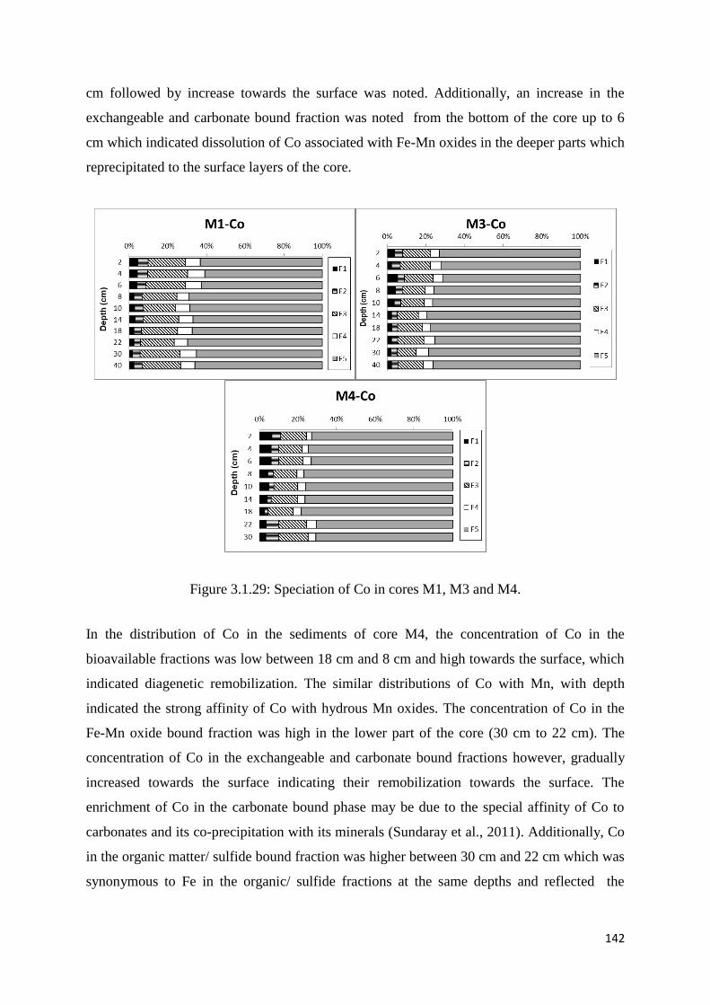
142
cm followed by increase towards the surface was noted. Additionally, an increase in the
exchangeable and carbonate bound fraction was noted from the bottom of the core up to 6
cm which indicated dissolution of Co associated with Fe-Mn oxides in the deeper parts which
reprecipitated to the surface layers of the core.
Figure 3.1.29: Speciation of Co in cores M1, M3 and M4.
In the distribution of Co in the sediments of core M4, the concentration of Co in the
bioavailable fractions was low between 18 cm and 8 cm and high towards the surface, which
indicated diagenetic remobilization. The similar distributions of Co with Mn, with depth
indicated the strong affinity of Co with hydrous Mn oxides. The concentration of Co in the
Fe-Mn oxide bound fraction was high in the lower part of the core (30 cm to 22 cm). The
concentration of Co in the exchangeable and carbonate bound fractions however, gradually
increased towards the surface indicating their remobilization towards the surface. The
enrichment of Co in the carbonate bound phase may be due to the special affinity of Co to
carbonates and its co-precipitation with its minerals (Sundaray et al., 2011). Additionally, Co
in the organic matter/ sulfide bound fraction was higher between 30 cm and 22 cm which was
synonymous to Fe in the organic/ sulfide fractions at the same depths and reflected the

143
partitioning of Co as a result of low Eh with depth along with formation of FeS2 (Evans et
al., 1988).
Between the three cores, higher Co in the exchangeable fraction was noted at M4, whereas
Co in the carbonate bound, Fe-Mn oxide bound and organic/sulfide bound fraction was high
at M1.
From the above, it was noted that the distribution and speciation of Co in sediments varied
with changes in pH, ionic strength and organic matter (Mahara and Kudo, 1981). Co was
precipitated to the sediments in the adsorbed state with oxides of iron and manganese or with
the crystalline sediments such as aluminosilicates and goethite. The higher content of Co in
the Fe-Mn oxides phase in sediments was due to adsorption of larger amount of Co to Fe-Mn
oxides (McLaren et al., 1986). In deeper oxygen depleted sediment layers, the lowering of
sediment redox potential and pH may have occurred which resulted in the reduction of iron
and manganese oxides. Consequently, the adsorbed Co was released by dissolution of the
oxides and thus increased Co mobility towards the surface and precipitation in the oxic layers
along with Fe-Mn oxides (Smith and Carson, 1981, Kim et al., 2006), resulting in enrichment
in the surface layers which was seen in all the three mudflat cores. Further, the considerable
amount of Co in the organic/ sulfide fraction was due to the formation of complexes with
fulvic and humic acids or other organic ligands but are however, less stable.
3.1. E .2e Copper
The concentration of Cu in the five fractions is in the order of F5>F4>F3>F2>F1 in core M1
which was collected from the upper middle estuary mudflat. Large quantity of Cu was
associated with the residual fraction ranging from 52.93 ppm to 73.58 ppm (average 59.02
ppm) that accounted for 61.83 % to 72.10 % (average 66.08 %). Among the bioavailable
fractions, considerable quantity of Cu was associated with the organic/ sulfide bound phases
with concentrations ranging from 20.38 ppm to 33.08 ppm (average 24.32 ppm) that
accounted for 21.86 % to 31.55 % (average 27.14 %). The concentration of Cu in the Fe-Mn
oxide fraction ranged from 2.95 ppm to 4.20 ppm (average 3.38 ppm) that accounted for 3.34
% to 4.31 % (average 3.79 %) whereas concentrations in the carbonate fraction ranged from
1.33 ppm to 1.73 ppm (average 1.53 ppm) that accounted for 1.41 % to 1.89 % (average 1.73
%). Least amount of Cu was found in the exchangeable fraction with a range of 1.00 ppm to
1.28 ppm (average 1.12 ppm) and accounted for 1.01 % to 1.51 % (average 1.27 %) of the
144
total of the five fractions. The concentration of Cu in core M3 varied in the order of
F5>F4>F3>F1>F2. The concentration of Cu in the residual phase ranged from 52.83 ppm to
67.98 ppm (average 61.50 ppm) that accounted for 76.23 % to 85.06 % (average 81.46 %).
Considerable amount of Cu however, was found in the bioavailable phases mainly in the
organic/ sulfide fraction concentrations ranged from 8.65 ppm to 13.80 ppm (average 10.63
ppm ) and accounted for 11.41 % to 19.91 % (average 14.11 %). The concentration in the Fe-
Mn oxide fraction ranged from 1.18 ppm to 2.38 ppm (average 1.66 ppm) that accounted for
1.70 % to 3.08 % (average 2.18 %) whereas the concentration of Cu in the exchangeable
fraction ranged from 0.53 ppm to 1.83 ppm (average 0.96 ppm) that accounted for 0.72 % to
2.37 % (average 1.26 %). Least quantity of Cu was noted in the carbonate bound fraction that
ranged from 0.63 ppm to 0.88 ppm (average 0.74 ppm) and accounted for 0.86 % to 1.12 %
(average 0.98 %). In core M4, the concentration of Cu varied in the order of
F5>F4>F3>F2>F1. Large quantity of Cu was associated with the residual phase ranging from
50.50 ppm to 78.18 ppm (average 61.07 ppm) which accounted for 80.90 % to 89.75 %
(average 86.36 %). The concentration of Cu in the organic/ sulfide bound fraction varied
form 5.60 ppm to 9.00 ppm (average 6.71 ppm) that accounted for 6.83 % to 14.42 %
(average 9.67 %) whereas Cu in the Fe-Mn oxide fraction ranged from 0.98 ppm to 1.60 ppm
(average 1.19 ppm) that accounted for 1.41 % to 2.28 % (average 1.70 %). Cu in the
carbonate bound fraction ranged from 0.98 ppm to 1.25 ppm (average 1.11 ppm) that
accounted for 1.23 % to 1.99 % (average 1.59 %). Least Cu concentrations were found in the
exchangeable phase, which ranged from 0.20 ppm to 0.68 ppm (average 0.47 ppm) and
accounted for 0.28 % to 1.04 % (average 0.67 %).
Overall, Cu in the sediments was enriched in the F5, F4 and F3 fractions followed by low
concentrations in the F2 and F1 fractions. Residual Cu in the mudflat sediments varied from
66.08 % to 86.36 %, highest being in core M4. The concentration of Cu in the organic
matter/ sulfide bound fraction ranged from 9.67 % to 27.14 %, highest being in core M1. Fe-
Mn oxide bound Cu content varied from 1.70 % to 3.79 %, with higher concentration in core
M1. Cu content in carbonate bound and exchangeable fraction varied from 1.59 % to 1.73 %
and 0.67 % to 1.72 % respectively, with higher concentrations in core M1 for both fractions.
In the distribution of Cu with depth in the five fractions of core M1 (Figure 3.1.30) Cu in the
residual fraction exhibited relatively uniform distribution except for higher values at 22 cm
and 14 cm. The organic/ sulfide fraction was the main repository for Cu among the
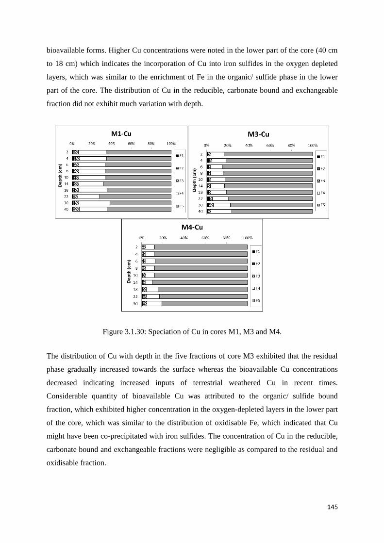
145
bioavailable forms. Higher Cu concentrations were noted in the lower part of the core (40 cm
to 18 cm) which indicates the incorporation of Cu into iron sulfides in the oxygen depleted
layers, which was similar to the enrichment of Fe in the organic/ sulfide phase in the lower
part of the core. The distribution of Cu in the reducible, carbonate bound and exchangeable
fraction did not exhibit much variation with depth.
Figure 3.1.30: Speciation of Cu in cores M1, M3 and M4.
The distribution of Cu with depth in the five fractions of core M3 exhibited that the residual
phase gradually increased towards the surface whereas the bioavailable Cu concentrations
decreased indicating increased inputs of terrestrial weathered Cu in recent times.
Considerable quantity of bioavailable Cu was attributed to the organic/ sulfide bound
fraction, which exhibited higher concentration in the oxygen-depleted layers in the lower part
of the core, which was similar to the distribution of oxidisable Fe, which indicated that Cu
might have been co-precipitated with iron sulfides. The concentration of Cu in the reducible,
carbonate bound and exchangeable fractions were negligible as compared to the residual and
oxidisable fraction.

146
From the distributions of Cu with depth in the five fractions of core M4, Cu in the residual
fractions increased towards the surface indicating the increased input of terrestrial material.
Higher bioavailable Cu concentrations were noted in the deep part of the core (18 cm to 30
cm) which decreased up to 14 cm. The high concentrations of Cu in the oxidisable phase in
the lower part of the core indicated the association of Cu with iron sulfides.
Overall, relatively high Cu concentration in the bioavailable phases was noted in the upper
middle estuary followed by lower middle and lower estuary. The enrichment of bioavailable
Cu in the upper middle estuary indicated that the source as anthropogenic probably from
marine transportation and shipbuilding activities wherein Cu is employed as an active
ingredient in antifouling paints for recreational and commercial vessels moored and
maintained in the estuary (Burton et al., 2005). High content of Cu in the residual fraction in
the estuarine system indicated that Cu was occluded within the crystal structure of
recalcitrant minerals and is not available to biota or due to diagenetic processes (Tessier et
al., 1979). Cu in the oxidisable fraction was due to the formation of stable organic complexes
(Stumm and Morgan, 1996). Bubb et al. (1991) reported that Cu tends to have a high affinity
for the clay/silt fraction. Thus, the higher proportion of Cu may be due to sorption to clay
minerals (Pickering, 1986; Massolo et al., 2012). The carbonate and exchangeable fractions
contained negligible concentrations of Cu.
3.1. E.2f Zinc
The concentration of Zn in core M1, varied in the order of abundance F5>F3>F4>F2>F1.
Large proportion of Zn was associated with the residual phase ranging from 58.43 ppm to
86.35 ppm (average 70.39 ppm) that accounted for 64.36 % to 72.00 % (average 68.37 %).
Considerable amount of Zn was associated with the bioavailable fractions. The concentration
of Zn in the Fe-Mn oxide fraction ranged from 15.50 ppm to 26.10 ppm (average 19.81 ppm)
that accounted for 16.68 % to 22.47 % (average 19.18 %) whereas, Zn in the organic/sulfide
bound fractions with concentrations varying between 8.08 ppm to 12.78 ppm (average 10.50
ppm) that accounted for 9.14 % to 11.72 % (average 10.19 %). Zn in the carbonate bound
fraction ranged from 0.98 ppm to 1.98 ppm (average 1.40 ppm) that accounted for 0.95 % to
1.93 % (average 1.36 %) whereas concentrations in the exchangeable fraction ranged from
0.63 ppm to 1.43 ppm (average 0.91 ppm) that accounted for 0.61 % to 1.35 % (average 0.89
%). In core M3, the concentration of Zn in the five fractions varied in the order of abundance
F5>F3>F4>F2>F1. The concentrations of Zn in the residual fraction varied between 61.53

147
ppm to 90.47 ppm (average 73.45 ppm) that accounted for 69.79 % to 82.55 % (average
76.77 %). Among the bioavailable fractions, Zn was mainly associated with the Fe-Mn oxide
fraction wherein its concentration ranged from 10.80 ppm to 14.40 ppm (average 13.18 ppm)
that accounted for 9.85 % to 16.78 % (average 13.96 %). Considerable amounts of Zn were
noted in the organic/ sulfide bound fraction wherein it ranged from 4.58 ppm to 8.30 ppm
(average 5.66 ppm) that accounted for 4.94 % to 8.41 % (average 5.93 %). Zn in the
carbonate fraction ranged from 1.23 ppm to 4.05 ppm (average 1.80 ppm) that accounted for
1.16 % to 4.51 % (average 1.92 %) whereas Zn in the exchangeable fraction ranged from
0.33 ppm to 4.05 ppm (average 1.34 ppm) that accounted for 0.40 % to 4.51 % (average 1.41
%) of the total of the five fractions. The concentration of Zn in core M4 varied in the order of
F5>F3>F4>F2>F1. The residual phase contained the highest Zn concentrations among the
five fractions, which ranged from 59.65 ppm to 104.78 ppm (average 80.25 ppm) that
accounted for 68.01 % to 84.67 % (average 78.02 %). Among the bioavailable phases, the Fe-
Mn oxide fraction was the main phase wherein Zn ranged from 11.38 ppm to 24.60 ppm
(average 14.74 ppm) that accounted for 10.26 % to 20.91 % (average 14.46 %). Zn
concentrations in the organic/ sulfide fraction varied between 2.98 ppm and 6.78 ppm
(average 3.86 ppm) that accounted for 2.75 % to 5.76 % (average 3.81 %). The
concentrations of Zn in the carbonate fraction ranged from 1.15 ppm to 4.85 ppm (average
2.14 ppm) that accounted for 0.99 % to 4.86 % (average 2.10 %) whereas concentrations in
the exchangeable fraction ranged from 1.10 ppm to 2.38 ppm (average 1.64 ppm) that
accounted for1.09 % to 2.35 % (average 1.62 %).
Overall, Zn followed the same order of abundance in the three mudflat cores of
F5>F3>F4>F2>F1. Further, Zn in the residual fraction varied from 68.37 % to 78.02 %,
highest being in core M4. The Fe-Mn oxide bound Zn in the mudflat sediments varied from
13.96 % to 19.18 % with higher concentrations in core M1. Zn content in the organic matter/
sulfide bound phase ranged from 3.81 % to 10.19 %, highest concentrations being in core
M1. Low content of carbonate bound and exchangeable Zn were noted in the mudflats values
varying from 1.36 % to 2.10 % and 0.89 % to 1.62 % respectively, being in core M4.
The distribution of Zn with depth (Figure 3.1.31) in five fractions of core M1 showed that Zn
was mainly present in the residual phase, which exhibited a fluctuating with an overall
decreasing distribution pattern towards the surface. The distribution of Zn in the bioavailable
phases showed a minor increase towards the surface similar to the distribution of bioavailable
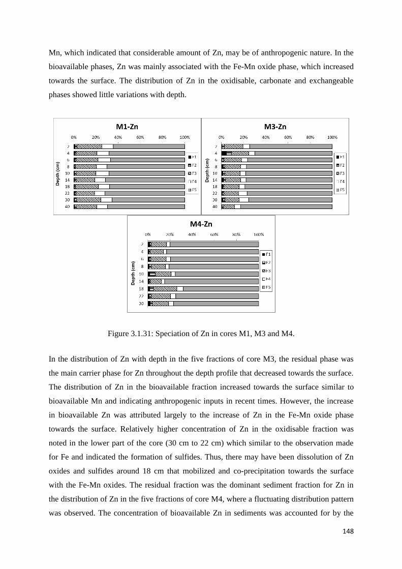
148
Mn, which indicated that considerable amount of Zn, may be of anthropogenic nature. In the
bioavailable phases, Zn was mainly associated with the Fe-Mn oxide phase, which increased
towards the surface. The distribution of Zn in the oxidisable, carbonate and exchangeable
phases showed little variations with depth.
Figure 3.1.31: Speciation of Zn in cores M1, M3 and M4.
In the distribution of Zn with depth in the five fractions of core M3, the residual phase was
the main carrier phase for Zn throughout the depth profile that decreased towards the surface.
The distribution of Zn in the bioavailable fraction increased towards the surface similar to
bioavailable Mn and indicating anthropogenic inputs in recent times. However, the increase
in bioavailable Zn was attributed largely to the increase of Zn in the Fe-Mn oxide phase
towards the surface. Relatively higher concentration of Zn in the oxidisable fraction was
noted in the lower part of the core (30 cm to 22 cm) which similar to the observation made
for Fe and indicated the formation of sulfides. Thus, there may have been dissolution of Zn
oxides and sulfides around 18 cm that mobilized and co-precipitation towards the surface
with the Fe-Mn oxides. The residual fraction was the dominant sediment fraction for Zn in
the distribution of Zn in the five fractions of core M4, where a fluctuating distribution pattern
was observed. The concentration of bioavailable Zn in sediments was accounted for by the

149
Fe-Mn oxide fraction wherein the Zn showed a peak at 18 cm followed by an almost uniform
distribution towards the surface. This decrease from 18 to 14 cm indicated redox mobilization
and increase at 10 cm indicated re-precipitation as oxides and similar to Mn and to a lesser
extent Fe. Zn in the organic/ sulfide fraction showed higher concentrations in the deeper
layers of the sediment core (30 cm to 18 cm) which may indicate that Zn incorporation into
sulfides.
Overall, relatively higher bioavailable fractions were noted in the lower estuary. High Zn
content in the reducible and oxidisable phases in the upper estuary indicated the role of Fe-
Mn oxides and organic matter in the removal of Zn from the water column to sediments.
The bioavailability of Zn in sediments was thus controlled by adsorption/desorption and
precipitation/dissolution mechanisms. Sorption was the dominant reaction governing
transport of zinc to sediments. Zn in the bioavailable fraction was associated with Fe and Mn
oxides (Lopez-Sanchez et al., 1996) due the ability of Zn to substitute for Fe in the structure
of oxide minerals (Stumm and Morgan, 1996). Zn in deeper reduced sediments below 22 cm
that contained sulfides might have incorporated in to sulfides. Due to anoxic conditions in
deeper sediments, dissolution of Fe-Mn oxides may have occurred, which mobilized the
adsorbed Zn and was thus re-precipitated near the surface in sub-oxic sediments. However,
large quantity of Zn was bound to the clastic detrital fraction of sediments resulting in overall
low mobility. The content of Zn in sediments therefore, depends on the chemical and
mineralogical properties of the sediment such as nature of parent rocks, sediment texture,
organic matter, and pH that determine the species and stability of Zn in the solid phase.
The speciation analysis of metals Fe, Mn, Cr, Co, Cu and Zn indicated that the main carrier
phase for Fe, Cr, Co, Cu and Zn was the residual phase suggesting a detrital control for these
metals whereas large quantity of Mn was associated with the non-residual or bioavailable
fraction indicating an anthropogenic source for Mn in addition to natural source. Among the
bioavailable fractions Fe, Mn, Co and Zn were mainly associated with the Fe-Mn oxide
phases which may have become soluble under the changing redox conditions whereas Cr and
Cu were associated with the organic matter/ sulfide fraction (except at S4 for Cr wherein
higher concentrations in Fe-Mn oxide phase were noted). Sediment organic matter is
important for the distribution of Cu and Cr in sediments as these metals have a strong affinity
to bind to the organic phases. The abundance of Fe, Cr, Co, Cu and Zn in the residual
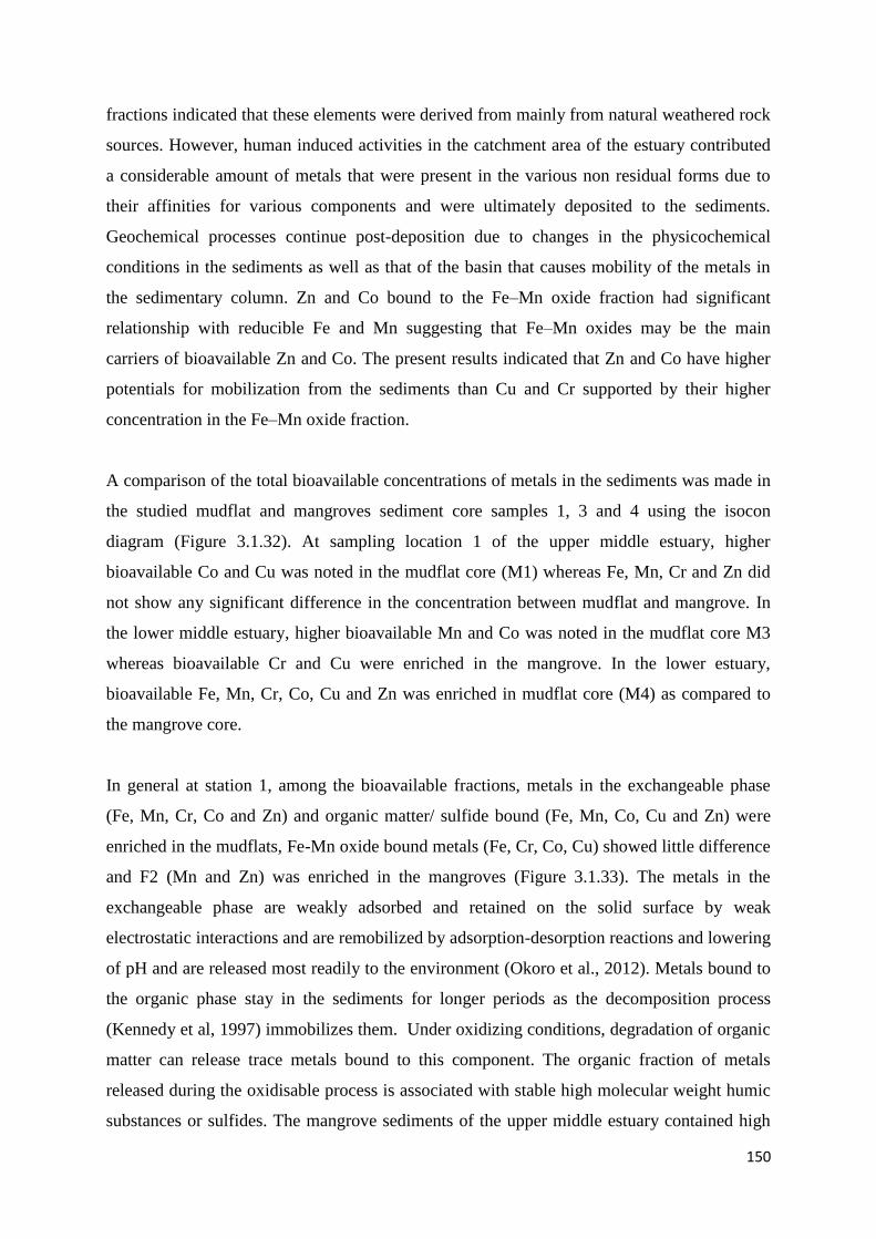
150
fractions indicated that these elements were derived from mainly from natural weathered rock
sources. However, human induced activities in the catchment area of the estuary contributed
a considerable amount of metals that were present in the various non residual forms due to
their affinities for various components and were ultimately deposited to the sediments.
Geochemical processes continue post-deposition due to changes in the physicochemical
conditions in the sediments as well as that of the basin that causes mobility of the metals in
the sedimentary column. Zn and Co bound to the Fe–Mn oxide fraction had significant
relationship with reducible Fe and Mn suggesting that Fe–Mn oxides may be the main
carriers of bioavailable Zn and Co. The present results indicated that Zn and Co have higher
potentials for mobilization from the sediments than Cu and Cr supported by their higher
concentration in the Fe–Mn oxide fraction.
A comparison of the total bioavailable concentrations of metals in the sediments was made in
the studied mudflat and mangroves sediment core samples 1, 3 and 4 using the isocon
diagram (Figure 3.1.32). At sampling location 1 of the upper middle estuary, higher
bioavailable Co and Cu was noted in the mudflat core (M1) whereas Fe, Mn, Cr and Zn did
not show any significant difference in the concentration between mudflat and mangrove. In
the lower middle estuary, higher bioavailable Mn and Co was noted in the mudflat core M3
whereas bioavailable Cr and Cu were enriched in the mangrove. In the lower estuary,
bioavailable Fe, Mn, Cr, Co, Cu and Zn was enriched in mudflat core (M4) as compared to
the mangrove core.
In general at station 1, among the bioavailable fractions, metals in the exchangeable phase
(Fe, Mn, Cr, Co and Zn) and organic matter/ sulfide bound (Fe, Mn, Co, Cu and Zn) were
enriched in the mudflats, Fe-Mn oxide bound metals (Fe, Cr, Co, Cu) showed little difference
and F2 (Mn and Zn) was enriched in the mangroves (Figure 3.1.33). The metals in the
exchangeable phase are weakly adsorbed and retained on the solid surface by weak
electrostatic interactions and are remobilized by adsorption-desorption reactions and lowering
of pH and are released most readily to the environment (Okoro et al., 2012). Metals bound to
the organic phase stay in the sediments for longer periods as the decomposition process
(Kennedy et al, 1997) immobilizes them. Under oxidizing conditions, degradation of organic
matter can release trace metals bound to this component. The organic fraction of metals
released during the oxidisable process is associated with stable high molecular weight humic
substances or sulfides. The mangrove sediments of the upper middle estuary contained high

151
organic matter to which metals probably bound easily and were deposited in the sediments.
Earlier researchers (Clark et al., 1998; Harbison, 1986; Machado et al., 2002) noted that
mangrove sediments are usually characterized by water logged anaerobic soils and have high
organic matter and sulfide contents.
3.1.F Comparison of sediment geochemical fractions in mangroves and mudflats
Figure 3.1.32: Isocon diagram of bioavailability of metals in mudflats versus mangroves.

152
Figure 3.1.33: Isocon diagram of species of metals in mudflats versus mangroves of station 1
of the upper middle estuary.
Low pH values are often observed in mangrove sediments compared to un-vegetated mudflat
sediments and are due to the microbial decomposition of mangrove litter and hydrolysis of
tannin in mangrove plants, which releases organic acids (Clark et al., 1998; Tam and Wong,
1998). Additionally, the extensive mangrove root system leads to increased oxygen
translocation into the sediment that facilitates pyrite oxidation leading to an increase in
sediment acidity (Thibodeau and Nickerson, 1986). Thus, oxidation of organic matter may
have occurred in mangrove sediments, which released the metals bound to organic matter as
compared to mudflats, which have less oxygen percolation into the sediments. These released
organic bound metals may have been bound to carbonates or diffused to the water column
during tidal inundation where they may have interacted with the sediment particles of the
mudflats through weak bonding reactions such as adsorption. The carbonate phase also tends

153
to adsorb metals when there is a reduction of Fe-Mn oxides and oxidation of organic matter
in the aquatic system. Thus, in the upper middle estuary, most metals were noted in the
exchangeable fraction in mudflats whereas due to less oxidizing conditions in the mudflats,
most metals may have been retained in the organic/ sulfide fraction.
Figure 3.1.34: Isocon diagram of species of metals in mudflats versus mangroves at station 3
of the lower middle estuary.
At station 3, carbonate bound metals (Fe, Mn, Cr, Co and Zn) and Fe-Mn oxide bound metals
(Fe, Mn and Cu) were enriched in the mudflats whereas organic matter/ sulfide bound metals
(Fe, Cr, Co, Cu and Zn) was enriched in the mangroves (Figure 3.1.34). The exchangeable
fraction was distributed in the mudflats for metals Fe, Cu and Zn and in mangrove for Mn,
Co and Cr. In the lower middle estuary, higher percentages of silt and clay were recorded in

154
the mangrove sediments, which may have led to the rapid deposition and preservation of
organic matter in the sediment. This might have led to compaction of the sediments with very
little amount of oxygen to percolate into the sediments and consequently resulted in low
oxidation of organic matter. Thus, most metals associated with the organic matter may have
been either preserved or converted/associated with sulfides. However, the lower content of
metals in the Fe-Mn oxide and carbonate bound fractions in the mangroves indicated that the
metals may have been mobilized through redox changes and diffused from the sediments.
Figure 3.1.35: Isocon diagram of species of metals in mudflats versus mangroves at station 4
of the lower estuary.
The lower middle estuary is tidally influenced than the upper middle estuary. The intertidal
flats are submerged and exposed for similar periods. As they are usually submerged during
mid tide, when tidal currents tend to reach their maximum speeds, sediment movement is

155
mainly controlled by these currents, but wave action may also be a factor especially when the
water is shallow during the low tide. Thus, the sediments are more disturbed physically as
compared to the upstream regions which may cause mobilization of metals from the anoxic
sediments and re-precipitated as oxides or loosely bound forms. The higher content of bulk
Mn in the mudflats may have trapped the metals that were mobilized from the mangrove
sediments.
At sampling location S4, exchangeable (Fe, Mn, Cr, and Co), Fe-Mn oxide bound metals
(Fe, Mn, Co, Cu and Zn) and organic matter/ sulfide bound metals (Fe, Mn. Cr, Co, Cu and
Zn) were enriched in the mudflats whereas carbonate bound metals (Fe, Cr, Co and Cu) was
enriched in mangroves (Figure 3.1.35). In the mangrove sediments, the presence of
calcareous material may have caused association of metals with the carbonates. Additionally
the higher sand content in the mangroves that comprise larger quartz particles which have
trigonal or hexagonal smooth crystal surfaces are unable to provide sufficient interaction area
resulting in higher solubility of metals (Guven and Akinci, 2013). Thus, the coarse sediments
may have provided low surface for retention of trace metals in loosely bound forms. The
higher content of fine sediments and organic matter in the mudflat sediments of the lower
estuary effectively trapped trace metals within the sediments. Thus, most metals were
adsorbed onto the active surface of clay minerals and organic matter. Studies by Jingchun et
al. (2010) found that mangrove sediments have higher salt content compared to mudflat and
as salt contents in downstream sites were significantly higher than those in upstream sites of
the estuary, which is attributed the salt accumulation in mangrove surface sediments due to
evaporation and increased daily tidal inundation in downstream site. The relative high salinity
in the lower estuary can inhibit the growth and activity of Sulfate reducing bacteria and thus
affect the reduction of SO4 2−
and the decomposition of organic matter in sediment, resulting
in metals bioavailability (Hou et al., 2013; Nizoli and Luiz-Silva, 2012). The high salinity in
the lower estuary also enhanced in the content of major cations (e.g., Na, K, Ca, Mg) that
compete for the sorption sites with heavy metals and decrease the binding of metals to humic
acids (Du Laing et al., 2009).
Thus, the accumulation and bioavailability of metals within sediments depends upon various
factors namely organic matter supply, sediment redox conditions, the rate of sulfate
reduction, salinity and sediment particle size (Zhang et al., 2014). As sediment
physicochemical parameters varied between vegetated and non-vegetated sediments along the

156
estuary, the partitioning and bioavailability of metals also changed. Studies by Almeida et al.
(2005) and Jacob and Otte (2004) showed that sediments colonized by plants exhibit stronger
oxidizing conditions than un-vegetated sediments. The surface sediment of mangroves may
desiccate during low tide, become aerated by biological processes such as bioturbation or
oxygen release from mangrove roots, resulting in oxidizing conditions (Clark et al., 1998).
However, due to the high density of roots and a short period of flooding in the mangrove
forest environment, the redox status of vegetated sediments may become the key limiting
factor for bioavailability of metals in mangroves. In tidal mudflats, where sediments are not
aerated by oxygen released from plant roots and higher moisture contents exist due to longer
periods of tidal inundation, organic matter content become the important limiting factor for
bioavailability of metals.
3.1. G Risk assessment
To understand the risk of metals to the sediment-associated benthic organisms, the total metal
content in the bioavailable fractions were compared with sediment quality values (SQV)
using SQuiRT (screening quick reference table) (Table 3.1.11).
Table 3.1.11: Screening Quick Reference table for metals in marine sediments (Buchman,
1999)
Metal Threshold
Effect level
(TEL)
Effects range
level (ERL)
Probable
Effects level
(PEL)
Effects
Range
Median
(ERM)
Apparent Effects
Threshold (AET)
Fe NA NA NA NA 22 % (Neanthes)
Mn NA NA NA NA 260 (Neanthes)
Cr 52.30 81.00 160 370 62 (Neanthes)
Co NA NA NA NA 10 (Neanthes)
Ni 15.9 20.9 42.8 51.6 110 (Echinoderm larvae)
Cu 18.7 34 108 270 390 (Microtox and Oyster
Larvae)
Zn 124 150 271 410 410 (Infaunal community)
Sediment guidelines
Threshold Effects
Level
Maximum concentration at which no effects are observed
Effects Range low 10th percentile values in effects
Probable Effects Level Lower limit of the range of concentrations at which adverse effects are
always observed
Effects Range Median 50th percentile value in effects
Apparent Effects
Level
Concentration above which biological indicator effects always observed

157
In the mangroves, the concentration of Fe in the bioavailable fractions and bulk metals at all
four stations fell below the Apparent Effects Threshold (AET) indicating no toxicity risk to
biota. Mn showed higher concentrations in the bulk sediment as well as in bioavailable
fractions than AET with relatively higher values in the upper middle estuary and Cumbharjua
canal sediments (Table 3.1.12). Cr concentrations were also higher than the AET in the bulk
sediments but lower in the bioavailable fractions. The concentration of Co in the bulk
sediments were higher than AET at all four locations, however, Co in the bioavailable
fractions was higher than the AET only at upper middle estuary and Cumbharjua canal and
posed a toxicity risk. Cu in bulk sediments was greater than the ERL in cores S1, S2 and S3
and greater than TEL at S4 whereas bioavailable Cu was greater than TEL only in core S1.
The concentration of Zn at all four mangrove cores was greater than TEL in the bulk
sediments whereas bioavailable Zn concentrations did not pose any toxicity risk.
Average concentrations of bulk metals, bioavailable fractions and exchangeable and
carbonate bound fraction of Fe, Mn, Cr, Co, Cu and Zn of mudflat sediments are presented in
table 3.1.13. In mudflats, the concentration of Fe in the bulk sediments and bioavailable
fractions fell below the AET and thus posed no toxicity risk. Mn concentrations in the bulk
and bioavailable fractions were greater than the AET with higher values in core M1. Cr
concentrations in the bulk sediments were greater than the AET; however, bioavailable Cr did
not pose any toxicity risk. Co in the bulk and bioavailable fractions were higher than the AET
and may pose considerable risk to biota. Cu concentrations in the bulk sediments were greater
than the ERL whereas bioavailable Cu was greater than the TEL in core M1. Zn
concentrations in the bulk sediments were greater than the TEL; however, bioavailable Zn did
not pose any risk to biota.

158
Table 3.1.12: Average concentrations of bulk metals, bioavailable fractions and exchangeable
and carbonate bound fraction of Fe, Mn, Cr, Co, Cu and Zn of mangrove sediments.
Mangrove Bulk
(ppm)
Bioavailable
fraction
Exchangeable + Carbonate
(ppm) (%)
Fe S1 108400 (10.84 %) 9418 (0.94%) 0.02
S2 145300 (14.53 %) 8399 (0.84%) 0.02
S3 105400 (10.54 %) 6908 (0.69%) 0.08
S4 91500 (9.15 %) 3943 (0.39%) 0.15
Mn S1 5181(>AET) 4993 (>AET) 47.33 (High risk)
S2 5122(>AET) 5327(>AET) 27.52 (Medium risk)
S3 2138(>AET) 1864( >AET) 41.46 (High risk)
S4 1153(>AET) 844 (>AET) 23.77(Medium risk)
Cr S1 274 (>AET) 26.75 1.07
S2 271(>AET) 23.35 1.17
S3 318(>AET) 41.01 1.5
S4 336(>AET) 25.04 1.38
Co S1 21.75(>AET) 14.73(>AET) 4.65
S2 22.85(>AET) 15.13(>AET) 5.18
S3 23.23(>AET) 8.98 7.49
S4 19.98(>AET) 9.67 11.86 (Medium risk)
Cu S1 45.90(>ERL) 27.82 (>TEL) 2.91
S2 36.26 (>ERL) 15.83 2.69
S3 42.11(>ERL) 15.6 2.4
S4 26.92 (>TEL) 6.59 5.6
Zn S1 144(>TEL) 33.21 2.05
S2 104(>TEL) 20.91 2.61
S3 127(>TEL) 22.9 2.76
S4 79.63(>TEL) 18.54 7.76
Risk assessment code was also used to evaluate the toxicity of the labile phases
(exchangeable + carbonate bound) of Fe, Mn, Cr, Co, Cu and Zn in sediments. In the
mangrove cores, Fe concentrations in the labile phases posed no risk to the organisms. Mn,
however, posed a medium risk in the lower estuary and canal sediments and a high risk in the
upper middle and lower middle estuary. Cr in the labile fractions posed a low risk to the biota
at all the four locations. Labile Co concentrations posed medium risk in the lower estuary.

159
The concentrations of labile Cu and Zn fell in the low risk category at all four mangrove
cores.
Table 3.1.13: Average concentrations of bulk metals, bioavailable fractions and exchangeable
and carbonate bound fraction of Fe, Mn, Cr, Co, Cu and Zn of mudflat sediments.
Mudflat Bulk sediments Bioavailable
Fraction
Exchangeable+
Carbonate
(ppm) %
Fe M1 10.50 9433 (0.94%) 0.05
M3 10.61 6771 (0.68%) 0.08
M4 10.44 4907 (0.49%) 0.24
Mn M1 5341(>AET) 4875 (>AET) 38.89 (High risk)
M3 3652(>AET) 3375 (>AET) 35.37 (High risk)
M4 2665(>AET) 2349(>AET) 32.73(High risk)
Cr M1 262(>AET) 25.63 1.03
M3 369(>AET) 36.53 0.97
M4 342(>AET) 37.07 2.39
Co M1 25.93(>AET) 16.74 (>AET) 7.33
M3 18.99(>AET) 11.45 (>AET) 6.50
M4 28.10(>AET) 10.67 (>AET) 8.20
Cu M1 46.48(>ERL) 30.35 (>TEL) 2.99
M3 39.74(>ERL) 13.99 2.25
M4 41.25(>ERL) 9.48 2.26
Zn M1 136(>TEL) 32.61 2.25
M3 124(>TEL) 21.98 3.34
M4 129(>TEL) 22.38 3.72
In the mudflat cores, concentration of labile Mn fell in the high risk category at all three
mudflat cores whereas labile Cr, Cu and Zn fell in the low risk category and labile Fe
concentrations fell in the no risk category.
Thus, the sources and level of input of Mn, Cr and Co should be continuously monitored to
understand the risk to the estuarine biota.

160
3.2 Seasonal Study
3.2. A Mangroves
3.2. A.1 Sediment components: pH, sand, silt, clay and TOC.
The range and average values of sediment components in mangrove sediments in the
premonsoon, monsoon and postmonsoon seasons are presented in table 3.2.1(a).
The pH of the mangrove sediments in the Zuari estuary during premonsoon, monsoon and
postmonsoon ranged from 6.54 to 7.22 (average 6.79), 6.05 to 6.85 (average 6.51) and 6.32 to
7.00 (average 6.68) respectively. Sand content in the estuary ranged from 0.97 % to 29.98 %
(average 9.57 %) during the premonsoon, 0.77 % to 30.04 % (average 9.23 %) during the
monsoon and 0.47 % to 35.57 % (average 10.51 %) during the postmonsoon. The silt content
in the estuary varied between 37.56 % and 56.15 % (average 44.18 %) during the
premonsoon, 8.48 % and 53.79 % (average 37.30 %) during the monsoon and 34.24 % and
46.38 % (average 39.01 %) during the postmonsoon. The dominant sediment size fraction
was clay ranging from 25.97 % to 60.52 % (average 46.26 %) during the premonsoon, 19.38
% to 89.84 % (average 53.47 %) during the monsoon and 27.52 % to 64.54 % (average 50.49
%) during the postmonsoon. The TOC content in the mangrove surface sediments during the
premonsoon, monsoon and postmonsoon ranged from 1.88 % to 2.60 % (average 2.26 %),
1.16 % to 3.06 % (average 2.27 %) and 1.46 % to 2.70 % (average 2.30 %) respectively.
Average silt was high during the premonsoon, clay during the monsoon, and sand and TOC
during the postmonsoon.
In the spatial distribution of sediment components, near neutral pH was noted in the estuary
sediments. The pH of the sediments at S1, S2 and S3 was low during monsoon followed by
higher values during premonsoon season and postmonsoon (Figure 3.2.1). Highest sand
content was noted in the lower estuary for all three seasons. Sand percentage decreased from
the upper middle estuary to the lower middle estuary followed by as large increase towards
the lower estuary. Considerable amount of sand was also noted in the Cumbharjua canal.
Highest silt content was noted in the Cumbharjua canal for all three seasons whereas lowest
values were noted in the upper middle estuary. The silt content increased from the upper
middle estuary to the lower estuary. Highest clay content was noted in the upper middle
estuary during the monsoon season. The clay content in the estuary decreased from the upper
middle estuary to the lower estuary.

161
Table 3.2.1: Range and average values of sediment components and bulk metals in mangrove sediments in the in the premonsoon, monsoon and
postmonsoon seasons.
Premonsoon Monsoon Postmonsoon Average Range Average Range Average Range (a) Sediment
components
pH 6.79 6.54 - 7.22 6.51 6.05- 6.85 6.68 6.32- 7.00 Sand (%) 9.57 0.97-29.98 9.23 0.77-30.04 10.51 0.47-35.57 Silt (%) 44.18 37.56-56.15 37.30 8.48-53.79 39.01 34.24-46.38 Clay (%) 46.26 25.97-60.52 53.47 19.38-89.84 50.49 27.52-64.54 TOC (%) 2.26 1.88-2.60 2.27 1.16-3.06 2.30 1.46-2.70 (b) Bulk metals Al (%) 9.78 8.73-10.97 9.54 5.87-11.34 10.40 8.11-11.22 Fe (%) 10.93 9.79-12.68 13.44 9.52-19.05 7.67 6.98-9.08 Mn (ppm) 3734 2286-4664 5325 1847-8983 5134 3331-6440 Cr (ppm) 353 264-542 242 147-305 274 246-300 Co (ppm) 22.5 17.00-29.50 16.94 10.00-24.50 18.44 15.75-21.25 Ni (ppm) 43.19 35.50-46.00 79.56 26.75-118.25 50.25 32.25-59.25 Cu (ppm) 39.25 30.00-48.25 113 74.25-174.25 108 101-117 Zn (ppm) 128 118-142 123 95.25-181 123 117-133
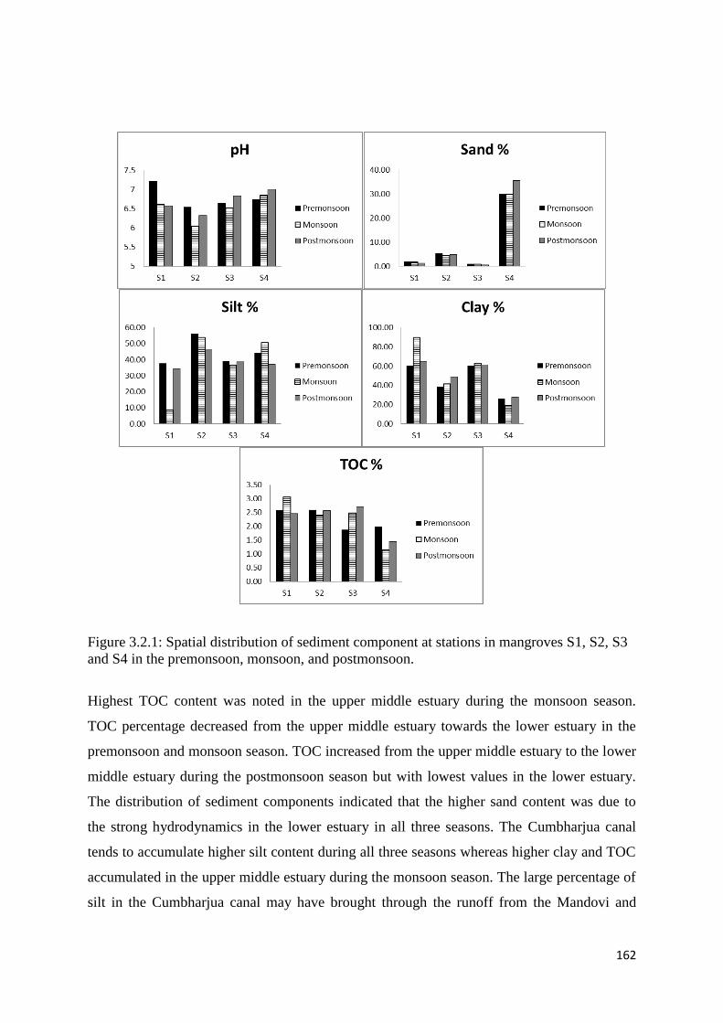
162
Figure 3.2.1: Spatial distribution of sediment component at stations in mangroves S1, S2, S3
and S4 in the premonsoon, monsoon, and postmonsoon.
Highest TOC content was noted in the upper middle estuary during the monsoon season.
TOC percentage decreased from the upper middle estuary towards the lower estuary in the
premonsoon and monsoon season. TOC increased from the upper middle estuary to the lower
middle estuary during the postmonsoon season but with lowest values in the lower estuary.
The distribution of sediment components indicated that the higher sand content was due to
the strong hydrodynamics in the lower estuary in all three seasons. The Cumbharjua canal
tends to accumulate higher silt content during all three seasons whereas higher clay and TOC
accumulated in the upper middle estuary during the monsoon season. The large percentage of
silt in the Cumbharjua canal may have brought through the runoff from the Mandovi and
163
deposited in the canal. Similarly, a large amount of organic matter accumulated in the upper
middle estuary along with clay during the monsoon season due to the increase in fluvial
runoff as a result of high rainfall and runoff.
3.2. A.2 Geochemistry of metals
The concentration of bulk metals in the mangrove sediments during premonsoon, monsoon
and postmonsoon are presented in table 3.2.1(b). The percentage of Al during the
premonsoon, monsoon and postmonsoon season varied from 8.73 % to 10.97 % (average
9.78 %), 5.87 % to 11.34 % (average 9.54 %) and 8.11 % to 11.22 % (average 10.40 %)
respectively. The concentrations of Fe ranged from 9.79 % to 12.68 % (average 10.93 %)
during the premonsoon, 9.52 % to 19.05 % (average 13.44 %) during the monsoon and 6.98
% to 9.08 % (average 7.67 %) during the postmonsoon. Mn content ranged from 2286 ppm to
4664ppm (average 3734 ppm) in the premonsoon, 1847 ppm to 8983 ppm (average 5325
ppm) in monsoon and 3331 ppm to 6440 ppm (average 5134 ppm) in the postmonsoon. Cr
concentrations varied from 264 ppm to 542 ppm (average 353.13 ppm) in the premonsoon
season, 147 ppm to 305 ppm (average 242 ppm) in the monsoon and 246 ppm to 300 ppm
(average 274 ppm) in the postmonsoon season. The concentrations of Co in the mangrove
sediments ranged from 17.00 ppm to 29.50 ppm (average 22.50 ppm) during the premonsoon,
10.00 ppm to 24.50 ppm (average 16.94 ppm) in the monsoon and 15.75 ppm to 21.25 ppm
(average 18.44 ppm) in the postmonsoon. Ni concentrations varied from 35.50 ppm to 46.00
ppm (average 43.19 ppm) in premonsoon, 26.75 ppm to 118.25 ppm (average 79.56 ppm) in
monsoon and 32.25 ppm to 59.25 ppm (average 50.25 ppm) in postmonsoon. Cu
concentrations varied from 30.00 ppm to 48.25 ppm (average 39.25 ppm) in the premonsoon,
74.25 ppm to 174 ppm (average 113 ppm) in monsoon and 101 ppm to 117 ppm (average 108
ppm) in postmonsoon. Zn content in the mangrove sediments ranged from 118 ppm to 115
ppm (average 128 ppm) in premonsoon, 95.25 ppm to 181 ppm (average 123 ppm) in the
monsoon and 117 ppm to 133 ppm (average 123 ppm) in the postmonsoon. Highest average
concentrations of Cr, Co and Zn were noted during the premonsoon, Fe, Mn, Ni and Cu
during the monsoon and Al during the postmonsoon.

164
Figure 3.2.2: Spatial distribution of bulk metals at mangrove stations S1, S2, S3 and S4 in the
premonsoon, monsoon and postmonsoon.
From the spatial distribution of metals in the mangroves of the Zuari estuary during the three
seasons (Figure 3.2.2), it was observed that during the premonsoon season, the concentrations
of Cr and Co increased along with sand from the upper middle to lower estuary. Fe along
with silt exhibited similar distribution pattern with higher value in the Cumbharjua canal. Ni,

165
Cu and Zn showed decrease along with clay and Mn, during the premonsoon season from the
upper middle to lower estuary with highest values in the upper middle estuary indicating their
association with clay and co-precipitation with Mn oxides. Following premonsoon,
concentration of most metals (Al, Fe, Mn, Ni, and Cu) increased, during the monsoon. The
highest concentrations of Cr, Cu and Zn along with clay, TOC Al and Fe, decreased from the
upper middle estuary towards the lower estuary during monsoon indicating source from the
catchment area and the role of aluminosilicates, TOC and Fe oxides that favoured the
retention of metals in sediments in the upstream region. Mn and Ni exhibited similar spatial
distribution trend with peak values in the Cumbharjua canal. In the postmonsoon season, Co,
Ni, Zn along with clay, TOC, Al and Mn exhibited similar distribution with overall
decreasing trend from the upper middle estuary towards the lower estuary with enrichment in
the lower middle estuary. Cr and Cu increased along with sand from the upper middle to
lower estuary indicating their association with coarse sediments. Fe and silt exhibited similar
spatial distribution pattern with peak values in the Cumbharjua canal.
It is thus apparent that metals show different associations with different seasons in the Zuari
estuary mangrove sediments. During the pre-monsoon (dry) season, the water in the estuarine
system remains well mixed and the intrusion of salt water is felt as far as 65 km upstream
(Qasim and Sengupta, 1981). In natural settings, flocculation of clay minerals occurs
dominantly in estuaries where fluvial (approximately 0 psu) waters are mixed with marine
waters (approximately 30 psu) (Sutherland et al., 2015). Fe and Mn are known to precipitate
at lower salinity through the formation of oxyhydroxides. Early removal of metals from
solution occurs on changes of physicochemical properties of water in the upstream, through
processes of flocculation and adsorption onto the active surfaces of clay minerals and Fe-Mn
oxyhydroxides that are deposited to the sediments. Thus most trace metals (Ni, Cu and Zn)
might have adsorbed on these oxides and clay particles and deposited in the upper middle
estuary. Cr and Co along with sand were enriched in the lower estuary and may have been
derived from local sources. Fe in the Cumbharjua canal either may have associated with the
silt sized particle or formed large clusters that fall in the silt size range.
During the monsoon season, the estuary becomes stratified and a salt wedge is formed which
extends up to about 12 km in the Zuari estuary. Heavy precipitation and land runoff in the
monsoon season bring about large changes in physicochemical properties of the estuarine
waters and the estuary becomes freshwater dominated. The large influx of terrestrial runoff

166
adds considerable suspended material to the estuary. Also abundant ore material is being
flushed into the estuary that is stored on the banks in the upstream region for loading onto
barges (Kessarkar et al., 2013). Since small rivers are originating from monsoon-dominated
and/or mountainous regions, their total TOC contribution to the estuarine system must be
substantial (Shynu et al., 2015). Thus high amount of aluminosilicates, Fe-Mn oxides and
organic matter in the estuary many have trapped the trace metals (Cr, Cu and Zn) in the upper
middle estuary. The monsoon season is followed by a recovery period during the
postmonsoon season wherein there is a reduction in fresh water influx. Higher accumulation
of trace metals, Co, Ni and Zn were related to the high content of fine sediments, organic
matter and Mn oxides in the upper middle estuary that were brought during the monsoons. Cr
and Cu were found to be enriched in the lower estuary and may be products of local
discharges.
3.2.B Mudflats
3.2.B.1 Sediment components: pH, sand, silt, clay and TOC
The range and average values of sediment components and metals in the mudflats along the
Zuari estuary in premonsoon, monsoon and postmonsoon are presented in table 3.2.2.
The pH of the mudflat sediments during the premonsoon, monsoon and postmonsoon season
ranged from 6.72 to 7.21 (average 6.93), 6.95 to 7.46 (average 7.21) and 6.75 to 7.05
(average 6.93) respectively. The percentage of sand varied from 1.90 % to 9.65 % (average
4.66 %) during the premonsoon, 3.93 % to 6.98 % (average 5.16 %) in the monsoon and 0.40
% to 3.57 % (average 1.83 %) in the postmonsoon. Silt varied from 36.54 % to 45.35 %
(average 41.37 %) in the premonsoon, 32.58 % to 50.45 % (average 40.78 %) in monsoon
and 36.27 % to 43.29 % (average 40.39 %) in the postmonsoon. Clay dominated the mudflat
sediments ranging from 45.00 % to 61.56 % (average 53.97 %) in premonsoon, 42.57 % to
62.83 % (average 54.06 %) in monsoon and 55.20 % to 60.16 % (average 57.79 %) in
postmonsoon. TOC exhibited minor seasonal variations ranging from 2.12 % to 2.75 %
(average 2.45 %) in premonsoon, 2.11 % to 3.03 % (average 2.60 %) in monsoon and 2.23 %
to 2.76 % (average 2.51 %) in postmonsoon.

167
Table 3.2.2 : Range and average values of sediment components and bulk metals in the mudflat sediments in the premonsoon, monsoon and
postmonsoon seasons.
Premonsoon Monsoon Postmonsoon
Average Range Average Range Average Range
(a) Sediment
components
pH 6.93 6.72-7.21 7.21 6.95-7.46 6.93 6.75-7.05
Sand (%) 4.66 1.90-9.65 5.16 3.93-6.98 1.83 0.40-3.57
Silt (%) 41.37 36.54-45.35 40.78 32.58-50.45 40.39 36.27-43.29
Clay (%) 53.97 45.00-61.56 54.06 42.57-62.83 57.79 55.20-60.16
TOC (%) 2.45 2.12-2.75 2.60 2.11-3.03 2.51 2.23-2.76
(b) Bulk metals Al (%) 10.29 10.12-10.51 10.38 8.65-11.58 10.93 10.29-11.45
Fe (%) 10.91 10.56-11.52 13.21 9.53-15.56 7.79 7.44-8.18
Mn (ppm) 4384 2747-5985 4892 3746-6251 5472 4243-6422
Cr (ppm) 335 306-385 235 176-271 262 242-296
Co (ppm) 26.50 19.50-32.25 15.00 6.75-19.75 18.75 14.50-23.00
Ni (ppm) 42.67 38.50-48.25 80.50 72.50-89.25 68.08 60.25-83.50
Cu (ppm) 41.42 37.50-48.50 122 97.50-166 111 99.50-120
Zn (ppm) 136 126-150 124 108-155 118 99.75-136

168
Figure 3.2.3: Spatial distribution of sediment components at stations M1, M3 and M4 in the
premonsoon, monsoon and postmonsoon.
The spatial distribution of sediment components in the mudflat sediments (Figure 3.2.3)
indicated that pH increased from the upper middle estuary to the lower estuary in the
premonsoon and monsoon season whereas higher pH were noted in the upper middle estuary
in the postmonsoon season. Sand content gradually increased towards the lower estuary in the
premonsoon and monsoon season owing to strong hydrodynamics but showed lower
percentage in the postmonsoon season. Silt content increased towards the lower estuary in
monsoon and postmonsoon seasons. In premonsoon season, silt was low in the lower middle
estuary. Clay exhibited higher percentage in the lower middle estuary during the premonsoon
whereas gradually decreased in clay content was observed from the upper middle estuary to
the lower estuary during the monsoon and postmonsoon. TOC was enriched in the upper

169
middle estuary mudflats in the premonsoon and monsoon, which decreased towards the lower
estuary whereas higher TOC was noted in the lower middle estuary in the postmonsoon
season.
3.2. B.2 Geochemistry of metals
The concentration of Al in mudflat sediments of the Zuari estuary ranged from 10.12 % to
10.51 % (average 10.29 %) in the premonsoon, 8.65 % to 11.58 % (average 10.38 %) in the
monsoon and 10.29 % to 11.45 % (average 10.93 %) in the postmonsoon (Table 3.2.2(b)). Fe
concentrations ranged from 10.56 % to 11.52 % (average 10.91 %) in premonsoon, 9.53 % to
15.56 % (average 13.21 %) in monsoon and 7.44 % to 8.18 % (average 7.79 %) in
postmonsoon. Mn content in the mudflat sediment varied from 2747 ppm to 5985 ppm
(average 4384 ppm) in premonsoon, 3746 ppm to 6251 ppm (average 4892 ppm) in monsoon
and 4243 ppm to 6422 ppm (average 5472 ppm) in postmonsoon. Cr concentrations in the
estuarine mudflats ranged from 306 ppm to 385 ppm (average 335 ppm) in premonsoon, 176
ppm to 271 ppm (average 235 ppm) in monsoon and 242 ppm to 296 ppm (average 262 ppm)
in postmonsoon. Co concentrations varied from 19.50 ppm to 32.25 ppm (average 26.50
ppm) in premonsoon, 6.75 ppm to 19.75 ppm (average 15.00 ppm) in monsoon and 14.50
ppm to 23.00 ppm (average 18.75 ppm) in postmonsoon. Ni concentrations varied from 38.50
ppm to 48.25 ppm (average 42.67 ppm) in premonsoon, 72.50 ppm to 89.25 ppm (average
80.50 ppm) in monsoon and 60.25 ppm to 83.50 ppm (average 68.08 ppm) in postmonsoon.
Cu content in sediments ranged from 37.50 ppm to 48.50 ppm (average 41.42 ppm) in
premonsoon, 97.50 ppm to 166 ppm (average 122 ppm) in monsoon and 99.50 ppm to 120
ppm (average 111 ppm) in postmonsoon. Zn concentrations varied from 126 ppm to 150 ppm
(average 136 ppm) in premonsoon, 108 ppm to 155 ppm (average 124 ppm) in monsoon and
99.75 ppm to 136 ppm (average 118 ppm) in postmonsoon. Highest average concentrations
of Cr, Co and Zn were noted in the premonsoon, Fe, Ni and Cu in the monsoon and Al and
Mn in postmonsoon.
When the spatial distribution of metals namely Cr, Co and Zn in the mudflat sediments
(Figure 3.2.4) of premonsoon season are considered, they varied similar to sand, silt and Al
distributions. These metals concentration decreased from the upper middle estuary to the
lower middle estuary followed by higher value in the lower estuary indicating that input of
Cr, Co and Zn was from the upstream regions of the estuary as well as from local point
sources in the lower estuary. Cu co-varied with Fe, Mn and TOC with highest values in the

170
upper middle estuary indicating that Cu was co-precipitated along with Fe-Mn oxides and
organic matter. Ni showed increase towards the lower estuary.
Figure 3.2.4: Spatial distribution of bulk metals at stations M1, M3 and M4 in the
premonsoon, monsoon and postmonsoon.
171
Following premonsoon, most metals (Al, Fe, Mn, Ni, Cu and Zn) concentrations considerably
increased. In monsoon, the spatial distribution of Cr, Ni, Cu and Zn co-varied with clay,
TOC, Al and Mn whereas decreasing trend towards the lower estuary was noted with highest
concentration in the upper middle estuary. Fe exhibited similar distribution to silt with
increasing trend from the upper middle estuary to the lower estuary. The spatial distribution
Co was noted to be similar to the distribution of sand where low content was noted in the
lower middle estuary and high values were noted in the lower estuary. In the postmonsoon
season, trace metal distribution of Cr, Co, Ni and Zn co-varied along with the distributions of
TOC with peak values in the lower middle estuary whereas the distribution of Cu was similar
to silt with higher concentration in the lower estuary. Al, Fe and Mn exhibited similar
distribution pattern to clay with a gradual decrease from the upper middle estuary to the
lower estuary.
The metal distribution showed seasonal differences in the mudflat sediments of the Zuari
estuary. In the premonsoon season, most trace metals Cr, Co, Ni, Cu and Zn are enriched in
the upper middle estuary sediments. This enrichment was due to the removal of metals during
early estuarine mixing of fluvial and seawater. Further, enrichment of metals towards the
upstream region of the estuary must be due to the proximity of the sampling location to the
metal sources namely mining and ore processing units located in the upper reaches of the
estuary, which could be a contributory factor for metals. Additionally, sediment grain size,
organic matter and hydrous Fe-Mn oxides played a considerable role in the adsorption and
deposition of metals to the sediments. In the monsoon, trace metals Co, Cr, Ni, Cu and Zn
were enriched in the upper middle estuarine sediments along with fine sediments, organic
matter and Mn oxides possible due to the large influx of fresh sedimentary material during
the monsoon land runoff and may be altering the elemental budget in the estuarine sediments
(Joseph and Srivastava, 1993). Significant amount of suspended /fine sediments and organic
matter are added to the estuary that favors binding of metals, during this season. In the
postmonsoon season, Cr, Co, Ni and Zn were enriched in the lower middle estuary along with
organic matter suggests that these metals may be associated with sewage or industrial
effluents. Dessai et al. (2009) made a similar observation, with higher enrichment of metals
in the postmonsoon season in the middle estuary. Most metals showed low concentrations in
the lower estuary. During the postmonsoon, the river discharge is negligible and saltwater
intrudes progressively into the estuarine channel (Shetye et al., 2007). The absence of
estuarine circulation and saltwater intrusion suppress turbulence and effectively removes fine

172
suspended sediments from the channel. Rao et al. (2011) reported that the turbidity maximum
occurs in the bay region of Zuari estuary due to resuspension fine sediments from the
marginal tidal flats and the combined the effect of wind-generated and ebb currents at neap
tide and their interaction with shallow bottom may have eroded and re-suspended sediments
from the shallow bathymetry.
3.2. C Geoaccumulation index
3.2. C.1 Mangroves
The geoaccumulation index was computed for metals, Fe, Mn, Cr, Co, Ni, Cu and Zn (Table
3.2.3). It was noted that in premonsoon, Igeo values of Mn and Cr fell in class 2 (Igeo 1-2) of
moderately polluted sediments, Fe in class 1(Igeo 0-1) of unpolluted to moderately polluted
sediments and Co, Ni, Cu and Zn in class 0 (Igeo <0) of unpolluted sediments. In the
monsoon season, Igeo values of Fe, Mn, Ni and Cu have shown considerable increase as
compared to premonsoon season whereas Cr, Co and Zn showed a decrease. Mn fell in class
3 (Igeo 2-3) of moderately to strongly polluted sediments, Fe, Cr, Ni and Cu values fell in
class1 (Igeo 0-1) of unpolluted to moderately polluted sediments and Co and Zn fell in class 0
(Igeo < 0) of unpolluted sediments. In the postmonsoon season, Fe, Mn, Ni, and Cu values
showed decrease as compared to monsoon season whereas Cr and Co Igeo values have
showed an increase. Mn fell in class 3 (Igeo 2-3) of moderately to strongly polluted
sediments, Cr fell in class 2 (Igeo1-2) of moderately polluted sediments, Fe and Cu fell in
class 1 (Igeo 0-1) of unpolluted to moderately polluted sediments and Co, Ni and Zn fell in
class 0 (Igeo<0) of unpolluted sediments.
Table 3.2.3: Geoaccumulation index of metals in mangrove sediments in premonsoon,
monsoon and postmonsoon.
Igeo-Mangrove
Fe Mn Cr Co Ni Cu Zn
Premonsoon 0.63 1.55 1.39 -0.34 -0.80 -0.78 -0.16
Monsoon 0.93 2.06 0.84 -0.75 0.09 0.74 -0.21
Postmonsoon 0.11 2.01 1.02 -0.63 -0.58 0.68 -0.21
3.2. C.2 Mudflats
Considerable seasonal variation was noted in the Igeo values in the mudflat sediments (Table
3.2.4). In premonsoon season, Igeo values of Mn and Cr fell in class 2 (Igeo 1-2) of
moderately polluted sediments, Fe in class 1 (Igeo 0-1) of unpolluted to moderately polluted

173
sediments and Co, Ni, Cu and Zn in class 0 (Igeo<0) of unpolluted sediments, similar to
mangrove sediments. In the monsoon season, Fe, Mn, Ni, and Cu Igeo values significantly
increased as compared to premonsoon season whereas Cr, Co and Zn decreased. Mn fell in
class 2 (Igeo 1-2) of moderately polluted sediments, Fe, Cr, Ni, and Cu fell in class 1 (Igeo 0-
1) of unpolluted to moderately polluted sediments and Co and Zn in class 0 (Igeo<0) of
unpolluted sediments.
Table 3.2.4 Geoaccumulation index of metals in mudflat sediments in premonsoon, monsoon
and postmonsoon.
Igeo-Mudflats
Fe Mn Cr Co Ni Cu Zn
Premonsoon 0.62 1.78 1.31 -0.10 -0.81 -0.70 -0.07
Monsoon 0.90 1.94 0.80 -0.93 0.10 0.85 -0.20
Postmonsoon 0.14 2.10 0.96 -0.60 -0.14 0.72 -0.27
In postmonsoon, Mn, Cr and Co Igeo values increased as compared to monsoon season
whereas Fe, Ni, Cu and Zn values decreased. Igeo value of Mn fell in class 3 (Igeo 2-3) of
moderately to strongly polluted sediments, Fe, Cr and Cu fell in class 1 (Igeo 0-1) of
unpolluted to moderately polluted sediments and Co and Ni in class 0 (Igeo <0) of unpolluted
sediments.
The considerable increase in Igeo values in the monsoon season was due to the increase in the
terrestrial runoff from the catchment area which adds considerable amount of trace metals of
anthropogenic origin into the estuary.
3.2. D Speciation of metals
3.2. D.1 Mangroves
3.2. D.1a Iron
The concentration Fe in the mangrove sediments of the Zuari estuary varied in the order of
abundance F5>F3>F4>F1>F2 in premonsoon, monsoon and post monsoon season. The
concentration of Fe in the residual phase varied from 63122 ppm to 85063 ppm (average
76718 ppm) in premonsoon, 58010 ppm to 92243 ppm (average 76959 ppm) in monsoon and
68060 ppm to 91495 ppm (average 80454 ppm) in postmonsoon. Fe in the reducible fraction
varied from 4403 ppm to 8453 ppm (average 6833 ppm) in premonsoon, 5948 ppm to 6465
ppm (average 6221 ppm) in monsoon and 4243 ppm to 6288 ppm (average 5381 ppm) in

174
postmonsoon. Fe content in the oxidisable fraction varied from 185 ppm to 750 ppm (average
566 ppm) in premonsoon, 374 ppm to 2154 ppm (average 1279 ppm) in monsoon and 62.50
ppm to 555 ppm (average 329 ppm) in postmonsoon. The concentrations of Fe n the
exchangeable phase ranged from 7.30 ppm to 113 ppm (average 52.33 ppm) in premonsoon,
2.10 ppm to 89.20 ppm (average 43.91 ppm) in monsoon and 5.73 ppm to 101 ppm (average
61.59 ppm) in postmonsoon. The least concentration of Fe was associated with the carbonate
fraction with concentrations ranging from 0.53 ppm to 1.68 ppm (average 1.24 ppm) in
premonsoon, 0.45 ppm to 6.78 ppm(average 2.81 ppm) in monsoon and 0.48 ppm to 87.13
ppm (average 23.28 ppm) in post monsoon. Highest average concentrations of reducible Fe
was noted in the premonsoon, oxidisable Fe in monsoon, and exchangeable, carbonate and
residual Fe in the post monsoon. Overall, highest bioavailable Fe (F1+F2+F3+F4) was noted
in the monsoon season (7547 ppm) followed by premonsoon (7452 ppm) and postmonsoon
(5795 ppm).
Figure 3.2.5: Spatial distribution of Fe speciation in mangrove sediments in the premonsoon,
monsoon and postmonsoon.
The spatial distribution of Fe in the five fractions (Figure 3.2.5) revealed that the bioavailable
Fe (sum of the first four fractions) was negligible in concentration as compared to the
residual fraction at all four mangrove sites. However, among bioavailable phases, higher Fe
in the Fe-Mn oxide bound fraction was noted at S1 and S2 in the premonsoon season as
compared to monsoon and postmonsoon seasons. Residual Fe during the premonsoon
increased from the upper middle estuary to the lower middle estuary followed by low
concentrations in the lower estuary whereas gradual decrease was noted in monsoon and
postmonsoon season towards the mouth of the estuary. Residual Fe was enriched at S2 in
premonsoon and monsoon season indicating that the significant amount of Fe was supplied to
the Zuari estuary, from the Mandovi estuary through the Cumbharjua canal, more
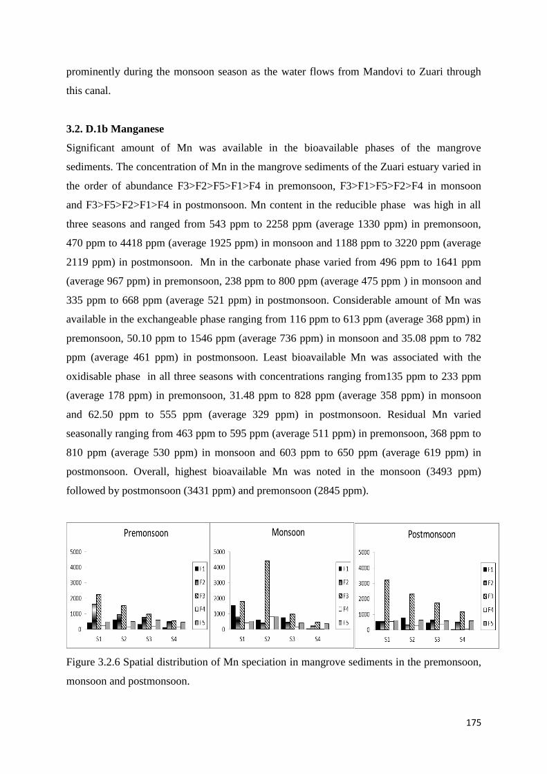
175
prominently during the monsoon season as the water flows from Mandovi to Zuari through
this canal.
3.2. D.1b Manganese
Significant amount of Mn was available in the bioavailable phases of the mangrove
sediments. The concentration of Mn in the mangrove sediments of the Zuari estuary varied in
the order of abundance F3>F2>F5>F1>F4 in premonsoon, F3>F1>F5>F2>F4 in monsoon
and F3>F5>F2>F1>F4 in postmonsoon. Mn content in the reducible phase was high in all
three seasons and ranged from 543 ppm to 2258 ppm (average 1330 ppm) in premonsoon,
470 ppm to 4418 ppm (average 1925 ppm) in monsoon and 1188 ppm to 3220 ppm (average
2119 ppm) in postmonsoon. Mn in the carbonate phase varied from 496 ppm to 1641 ppm
(average 967 ppm) in premonsoon, 238 ppm to 800 ppm (average 475 ppm ) in monsoon and
335 ppm to 668 ppm (average 521 ppm) in postmonsoon. Considerable amount of Mn was
available in the exchangeable phase ranging from 116 ppm to 613 ppm (average 368 ppm) in
premonsoon, 50.10 ppm to 1546 ppm (average 736 ppm) in monsoon and 35.08 ppm to 782
ppm (average 461 ppm) in postmonsoon. Least bioavailable Mn was associated with the
oxidisable phase in all three seasons with concentrations ranging from135 ppm to 233 ppm
(average 178 ppm) in premonsoon, 31.48 ppm to 828 ppm (average 358 ppm) in monsoon
and 62.50 ppm to 555 ppm (average 329 ppm) in postmonsoon. Residual Mn varied
seasonally ranging from 463 ppm to 595 ppm (average 511 ppm) in premonsoon, 368 ppm to
810 ppm (average 530 ppm) in monsoon and 603 ppm to 650 ppm (average 619 ppm) in
postmonsoon. Overall, highest bioavailable Mn was noted in the monsoon (3493 ppm)
followed by postmonsoon (3431 ppm) and premonsoon (2845 ppm).
Figure 3.2.6 Spatial distribution of Mn speciation in mangrove sediments in the premonsoon,
monsoon and postmonsoon.

176
The spatial distribution of Mn in the five fractions is presented in figure 3.2.6. The
concentration of Mn in the bioavailable fractions exhibited significant variations across the
three seasons. Exchangeable Mn exhibited a decreasing trend from the S1 to S4 with peak
values at S2 in the premonsoon and postmonsoon seasons. However, in the monsoon season,
there was a considerable increase in exchangeable Mn at S1 and S3. Carbonate bound Mn
showed a decreasing trend from S1 to S4 during the premonsoon season followed by lower
concentrations during the monsoon season and enrichment at S3 and S4 in postmonsoon
season. Most seasonal variability was noted for the Fe-Mn oxide fraction. The concentration
of reducible Mn decreased from S1 to S4 in the premonsoon and postmonsoon, with
relatively higher values during the postmonsoon. In monsoon, lower concentrations were
noted at S1 and S4 whereas enrichment at S2 was noted. Oxidisable Mn concentrations were
very low in premonsoon season, followed by increase at S1 and S2 in the monsoon and
increase at S1 and S3 in postmonsoon. Residual Mn exhibited little variation with seasons.
The upstream regions of the Zuari estuary have high Mn content due to the ore bearing
landmass (Zingde et al., 1976) and storage of ores on banks for transportations. Leachates
from the stored ore enter into the estuarine waters and are removed to the sediments as oxides
through processes of precipitate and flocculation of encountering saline waters in the estuary.
Thus, most Mn is removed in the upstream regions of the estuary resulting in enrichment in
sediments. In the monsoon season, due to increase in fresh water input to the estuary, the Mn
oxides formed in the sediments may undergo partial dissolution resulting in lower
concentrations in the Fe-Mn oxide fraction and enrichment in the labile fractions
(exchangeable and carbonate bound). Further, when there is heavy influx of fresh water from
the river, the estuarine sediments may be exchanging part of the exchangeable phase of the
metals of the water (Ouseph, 1987). A large amount of Mn enters into the estuary through run
off and accumulates in the sediments from anthropogenic sources. This was also reported
earlier. Additionally, the enrichment of reducible Mn in the Cumbharjua canal indicated large
contribution of Mn from the Mandovi estuary to the Zuari estuary through the canal. In the
postmonsoon season, due to decreasing fluvial discharge and with intrusion of sea water, the
Mn re-precipitates as oxides in the estuary.
3.2. D.1c Chromium
Cr was less associated with the bioavailable phase and exhibited little spatial variability in all
three seasons. The abundance of Cr in the five fractions varied in the order of abundance

177
F5>F4>F3>F1>F2 in premonsoon, monsoon and postmonsoon seasons. Most Cr was
associated with the residual fraction ranging from 153 ppm to 240 ppm (average 193 ppm) in
premonsoon, 171 ppm to 236 ppm (average 206 ppm) in monsoon and 195 ppm to 257 ppm
(average 220 ppm) in postmonsoon. However, among the bioavailable phases, considerable
amount of Cr was associated with the oxidisable phase varying from 12.08 ppm to 25.60 ppm
(average 16.85 ppm) in premonsoon, 7.28 ppm to 13.23 ppm (average 11.31 ppm ) in
monsoon and 8.10 ppm to 14.00 ppm (average 11.81 ppm) in postmonsoon. Cr in the
reducible phase ranged from 9.80 ppm to 11.95 ppm (average 10.68 ppm) in premonsoon,
9.08 ppm to 12.30 ppm (average 11.13 ppm) in monsoon and 9.13 ppm to 10.78 ppm
(average 9.93 ppm) in postmonsoon. Low concentrations of Cr was found in the
exchangeable phase that varied from 0.95 ppm to 2.38 ppm (average 1.91 ppm) in
premonsoon, 0.60 ppm to 0.83 ppm (average 0.68 ppm) in monsoon and 0.73 ppm to 1.33
ppm (average 1.06 ppm) in postmonsoon. Negligible concentration was noted in the
carbonate bound fraction ranging from 1.03 ppm to 1.65 ppm (average 1.32 ppm) in
premonsoon, 0.18 ppm to 0.68 ppm (average 0.33 ppm) in monsoon and 0.15 ppm to 0.73
ppm (average 0.36 ppm) in postmonsoon. Highest concentrations of exchangeable, carbonate
bound and oxidisable Cr was noted in premonsoon, reducible Cr in monsoon and residual Cr
in postmonsoon. Overall, highest bioavailable Cr was noted in premonsoon (30.77 ppm),
followed by monsoon (23.45 ppm) and postmonsoon (23.15 ppm).
Figure 3.2.7: Spatial distribution of Cr speciation in mangrove sediments in the premonsoon,
monsoon and postmonsoon.
The spatial distribution of bioavailable Cr across all three seasons showed little variations
(Figure 3.2.7). Cr in the residual phase was highest in the upper estuary followed by the
lower estuary and with lowest concentrations in the Cumbharjua canal during premonsoon. In
178
monsoon, residual Cr concentrations increased in the Cumbharjua canal and lower middle
estuary and decreased in the lower estuary. In postmonsoon, the concentration of residual Cr
was noted to increase considerably in the lower estuary.
As large Cr is bound in the mineral lattice form, minor amount of Cr is available for mobility
in the estuarine mangrove sediments. It was noted that during premonsoon season, most Cr
was supplied from the upstream regions of the estuary whereas enrichment in the lower
estuary indicated that a small fraction of Cr might be supplied from local sources like harbor,
barge building, etc. In the monsoon, enrichment of Cr in the Cumbharjua canal indicated
input of considerable amount of Cr from the Mandovi estuary to the Zuari estuary. The
decrease in the lower estuary suggested that Cr might have been re-suspended under
influence of strong wind induced waves and may have deposited in the lower middle estuary.
In the postmonsoon season, increase in the Cr in the lower estuary may be due to increasing
marine influx that transports Cr into the estuary, from harbor.
3.2. D.1d Cobalt
The concentration of bioavailable Co in mangrove sediments was considerably low as
compared to the residual fraction in all three seasons. The abundance of Co varied in the
order of F5>F3>F4>F2>F1 in premonsoon, F5>F4>F3>F2>F1 in monsoon, and
postmonsoon. The concentration of Co in the residual fraction varied from 26.48 ppm to
35.78 ppm (average 31.61 ppm) in premonsoon, 17.48 ppm to 35.95 ppm (average 28.81
ppm) in monsoon and 27.55 ppm to 36.40 ppm (average 32.27 ppm) in postmonsoon. The
concentration range for reducible Co was from 4.48 ppm to 9.75 ppm (average 7.48 ppm) in
premonsoon, 6.55 ppm to 11.43 ppm (average 6.82 ppm) in monsoon and 4.93 ppm to 9.33
ppm (Average 7.61 ppm) in postmonsoon. The Co associated with the organic matter/ sulfide
bound fraction varied from 1.05 ppm to 2.88 ppm (average 1.98 ppm) in premonsoon, 7.28
ppm to 13.23 ppm (average 11.31 ppm) in monsoon and 8.10 ppm to 14.00 ppm (average
11.81 ppm) in postmonsoon. Smaller quantity of Co was found in the labile fractions in all
three seasons. Carbonate bound Co varied from 1.43 ppm to 2.08 ppm (average 1.64 ppm) in
premonsoon, 1.40 ppm to 2.43 ppm (average 1.94 ppm) in monsoon and 1.13 ppm to 1.78
ppm (average 1.44 ppm) in postmonsoon. Least Co content was found in the exchangeable
fraction ranging from 0.60 ppm to 2.20 ppm (average 1.43 ppm) in premonsoon, 0.88 ppm to
1.13 ppm (average 1.01 ppm) in monsoon and 0.65 ppm to 1.60 ppm (average 1.12 ppm) in
postmonsoon. Highest average Co content in the exchangeable was noted in the premonsoon,

179
carbonate bound Co in the monsoon season and reducible, oxidisable, and residual Co in the
postmonsoon season. Overall, bioavailability of Co was high in the monsoon (22.88 ppm)
followed by postmonsoon (21.99 ppm) and premonsoon (12.53 ppm) seasons.
Figure 3.2.8: Spatial distribution of Co speciation in mangrove sediments in the premonsoon,
monsoon, and postmonsoon.
In the spatial distribution of Co in the five fractions, large seasonal variability was observed
in mangrove sediments (Figure 3.2.8). Exchangeable and carbonate bound Co maintained low
concentrations in all the three seasons at each mangrove location. However, relatively higher
exchangeable concentrations were noted in the premonsoon. Fe-Mn bound Co exhibited a
decreasing trend from S1 to S4 with peak values at S2 in all three seasons. Co in the organic
matter/ sulfide bound fraction exhibited large seasonal variations. Low carbonate bound Co
concentrations were noted in the premonsoon season. However, considerable increase in
oxidisable Co was observed in monsoon and postmonsoon seasons. The concentration of
residual Co at S1 was relatively constant in all the three seasons whereas other stations
showed variations. Residual concentrations were low during premonsoon at S2 and monsoon
and postmonsoon seasons at S4.
Most bioavailable Co in the mangrove sediments was associated with the Fe-Mn oxide and
organic matter/ sulfide bound phases. Similar enrichment of organic matter bound Mn in the
monsoon season indicated that the chemistry of Co and Mn in the estuary are closely related
and may be possibly linked to the same anthropogenic source.

180
3.2. D.1e Copper
Cu in the sediments of the Zuari estuary showed little seasonal variations in the bioavailable
fractions. The abundance of Cu in the five fraction varied in the order of F5>F4>F3>F2>F1
in premonsoon, F5>F4>F3>F1>F2 in monsoon and F5>F4>F1>F3>F1 in postmonsoon.
Large amount of Cu was associated with the residual fraction ranging from 49.50 ppm to 146
ppm (average 77.78 ppm) in premonsoon, 69.88 ppm to 202 ppm (average 115 ppm) in
monsoon and 56.40 ppm to 89.08 ppm (average 68.69 ppm) in postmonsoon. Among the
bioavailable fractions, Cu was mainly associated with the organic matter/sulfide fractions
with concentrations ranging from 4.60 ppm to 18.58 ppm (average 11.65 ppm) in
premonsoon, 6.28 ppm to 48.95 ppm (average 18.91 ppm) in monsoon and 8.58 ppm to 18.95
ppm (average 13.66 ppm) in postmonsoon. Cu content in the Fe-Mn oxide bound fraction
varied from 1.10 ppm to 2.60 ppm (average 1.72 ppm) in premonsoon, 2.43 ppm to 5.33 ppm
(average 3.79 ppm) in monsoon and 2.20 ppm to 2.80 ppm (average 2.64 ppm) in
postmonsoon. Carbonate bound Cu ranged from 0.78 ppm to 1.53 ppm (average 1.07 ppm) in
premonsoon, 1.23 ppm to 1.60 ppm (average 1.47 ppm) in monsoon and 1.43 ppm to 1.75
ppm (average 1.57 ppm) in postmonsoon. The concentration of exchangeable Cu varied from
0.65 ppm to 1.33 ppm (average 1.01 ppm) in monsoon, 1.10 ppm to 4.08 ppm (average 2.59
ppm) in monsoon and 2.00 ppm to 5.18 ppm (average 3.72 ppm) in postmonsoon. Highest
concentrations of exchangeable and carbonate bound Cu was noted in the postmonsoon and
Fe-Mn oxide bound, organic matter/sulfide bound and residual Cu in the monsoon. In
general, elevated concentrations of bioavailable Cu were noted in the monsoon (26.76 ppm)
followed by postmonsoon (21.59 ppm) and least in the premonsoon (15.44ppm).
Figure 3.2.9: Spatial distribution of Cu speciation in mangrove sediments in the premonsoon,
monsoon and postmonsoon.
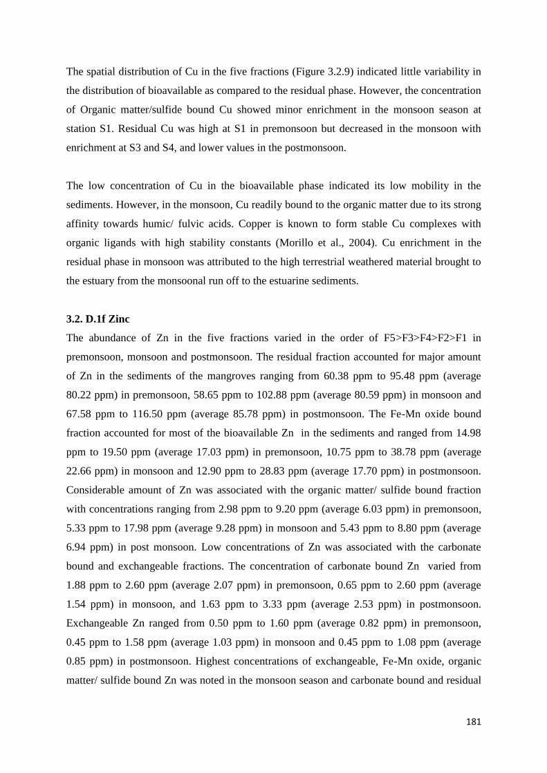
181
The spatial distribution of Cu in the five fractions (Figure 3.2.9) indicated little variability in
the distribution of bioavailable as compared to the residual phase. However, the concentration
of Organic matter/sulfide bound Cu showed minor enrichment in the monsoon season at
station S1. Residual Cu was high at S1 in premonsoon but decreased in the monsoon with
enrichment at S3 and S4, and lower values in the postmonsoon.
The low concentration of Cu in the bioavailable phase indicated its low mobility in the
sediments. However, in the monsoon, Cu readily bound to the organic matter due to its strong
affinity towards humic/ fulvic acids. Copper is known to form stable Cu complexes with
organic ligands with high stability constants (Morillo et al., 2004). Cu enrichment in the
residual phase in monsoon was attributed to the high terrestrial weathered material brought to
the estuary from the monsoonal run off to the estuarine sediments.
3.2. D.1f Zinc
The abundance of Zn in the five fractions varied in the order of F5>F3>F4>F2>F1 in
premonsoon, monsoon and postmonsoon. The residual fraction accounted for major amount
of Zn in the sediments of the mangroves ranging from 60.38 ppm to 95.48 ppm (average
80.22 ppm) in premonsoon, 58.65 ppm to 102.88 ppm (average 80.59 ppm) in monsoon and
67.58 ppm to 116.50 ppm (average 85.78 ppm) in postmonsoon. The Fe-Mn oxide bound
fraction accounted for most of the bioavailable Zn in the sediments and ranged from 14.98
ppm to 19.50 ppm (average 17.03 ppm) in premonsoon, 10.75 ppm to 38.78 ppm (average
22.66 ppm) in monsoon and 12.90 ppm to 28.83 ppm (average 17.70 ppm) in postmonsoon.
Considerable amount of Zn was associated with the organic matter/ sulfide bound fraction
with concentrations ranging from 2.98 ppm to 9.20 ppm (average 6.03 ppm) in premonsoon,
5.33 ppm to 17.98 ppm (average 9.28 ppm) in monsoon and 5.43 ppm to 8.80 ppm (average
6.94 ppm) in post monsoon. Low concentrations of Zn was associated with the carbonate
bound and exchangeable fractions. The concentration of carbonate bound Zn varied from
1.88 ppm to 2.60 ppm (average 2.07 ppm) in premonsoon, 0.65 ppm to 2.60 ppm (average
1.54 ppm) in monsoon, and 1.63 ppm to 3.33 ppm (average 2.53 ppm) in postmonsoon.
Exchangeable Zn ranged from 0.50 ppm to 1.60 ppm (average 0.82 ppm) in premonsoon,
0.45 ppm to 1.58 ppm (average 1.03 ppm) in monsoon and 0.45 ppm to 1.08 ppm (average
0.85 ppm) in postmonsoon. Highest concentrations of exchangeable, Fe-Mn oxide, organic
matter/ sulfide bound Zn was noted in the monsoon season and carbonate bound and residual

182
Zn in postmonsoon season. Overall, high bioavailable Zn was found in the monsoon (34.50
ppm) followed by postmonsoon (28.02 ppm) and premonsoon (25.95 ppm).
Figure 3.2.10: Spatial distribution of Zn speciation in mangrove sediments in the
premonsoon, monsoon and postmonsoon.
The spatial distribution of Zn in the five fractions revealed that the exchangeable and
carbonate bound fraction maintained very low concentrations in all three seasons (Figure
3.2.10). The Fe-Mn oxide fractions were constant in all four stations during the premonsoon.
However, during the monsoon season, an increase in the Fe-Mn oxide bound Zn at stations
S1 and S4 and during postmonsoon at station S4 was noted. The organic matter/ sulfide
bound Zn showed high values in the monsoon season at station S1. Residual Zn considerably
increased at stations S1 and S2 during monsoon and high at station S3 during premonsoon
and postmonsoon.
Zn is known to complex with humic/fulvic acid and adsorb on Fe-Mn oxyhydroxides in the
aquatic environment. The large influx of monsoonal runoff facilitated binding of Zn to
particulate matter and was removed to the sediments increasing the concentrations. Most
mineral bound Zn tends to settle in the upstream areas upon entering the estuary.
3.2. D.2 Mudflats
3.2. D.2a Iron
The percentage abundance of Fe in the five fractions varied in the order of F5>F3>F4>F1>F2
in the premonsoon, monsoon and postmonsoon seasons. The dominant fraction of Fe was the
residual fraction with concentrations ranging from 51215 ppm to 76233 ppm (average 64343
ppm) in premonsoon, 74648 ppm to 84248 ppm (average 77883 ppm) in monsoon and 76668
ppm to 88073 ppm (average 81171 ppm) in postmonsoon. Fe in the bioavailable phase was

183
most abundant in the Fe-Mn oxide bound fraction with concentrations ranging from 4750
ppm to 8285 ppm (average 6140 ppm) in premonsoon, 6183 ppm to 6345 ppm (average 6247
ppm) in monsoon and 4385 ppm to 6043 ppm (average 5012 ppm) in postmonsoon.
Considerable amount of Fe was associated with oxidisable phase ranging from 154 ppm to
1125 ppm (average 597 ppm) in premonsoon, 1534 ppm to 3421 ppm (average 2456 ppm) in
monsoon and 303 ppm to 513 ppm (average 417 ppm) in postmonsoon. Low concentrations
of Fe were associated with the exchangeable phase ranging from 20.60 ppm to 88.70 ppm
(average 54.12 ppm) in premonsoon, 5.28 ppm to 48.93 ppm (21.30 ppm) in monsoon and
7.18 ppm to 104.48 ppm (average 40.21 ppm) in postmonsoon. The carbonate bound Fe
ranged from 0.48 ppm to 17.83 ppm (average 7.16 ppm) in premonsoon, 0.63 ppm to 0.78
ppm (average 0.73 ppm) in monsoon and 0.35 ppm to 34.3 ppm (average 1.53 ppm) in
postmonsoon. Highest average concentration of exchangeable and carbonate bound Fe was
noted in premonsoon, reducible and oxidisable Fe in monsoon and residual Fe in
postmonsoon. In general, highest bioavailable Fe was noted during the monsoon season
(8724 ppm) followed by premonsoon (6798 ppm) and postmonsoon (5471 ppm).
Figure 3.2.11: Spatial distribution of Fe speciation in mudflat sediments in the premonsoon,
monsoon and postmonsoon.
The spatial variation of Fe in the five fractions showed that bioavailable Fe concentration was
very low as compared to the residual fraction (Figure 3.2.11). However, Fe in the reducible
phase exhibited a decreasing trend from M1 to M4 in premonsoon and monsoon seasons. Fe
in the residual fraction was low at M1 and M4 during the premonsoon whereas residual Fe at
M1 and M4 increased during monsoon and post monsoon. During monsoon season, a large
amount of terrestrial Fe is added which is transported and deposited in the estuary. The
concentration of residual Fe at M3 was almost constant in all three seasons indicating that the

184
intensive estuarine mixing at the lower middle estuary facilitates largely uniform
sedimentation processes.
3.2. D.2b Manganese
Mn in mudflat sediments exhibited large seasonal variability with the five fractions of
sediments. The concentration of Mn varied in the order of abundance F3>F2>F5>F1>F4 in
premonsoon, F3>F1>F2>F5>F4 in monsoon and F3>F2>F5>F4>F1 in postmonsoon. Most
bioavailable Mn was associated with the reducible fraction in all the three seasons ranging
from 1110 ppm to 2703 ppm (average 2042 ppm) in premonsoon, 975 ppm to 2203 ppm
(average 1536 ppm) in monsoon and 1785 ppm to 3083 ppm (average 2310 ppm) in
postmonsoon. Mn in the carbonate bound fraction ranged from 780 ppm to 1450 ppm
(average 1096 ppm) in premonsoon, 538 ppm to 728 ppm (average 607 ppm) in monsoon and
608 ppm to 893 ppm (709 ppm) in postmonsoon. Exchangeable Mn concentrations varied
from 83.83 ppm to 764 ppm (average 385 ppm) in premonsoon, 270 ppm to 1020 ppm
(average 613 ppm) in monsoon and 130 ppm to 475 ppm (average 314 ppm) in postmonsoon.
Least bioavailable Mn was associated with the oxidisable phase with concentrations ranging
from 189 ppm to 378 ppm (average 307 ppm) in premonsoon, 183 ppm to 458 ppm (average
287 ppm) in monsoon and 303 ppm to 513 ppm (average 417 ppm) in postmonsoon. The
concentration of Mn in the residual phase ranged from 483 ppm to 620 ppm (average 539
ppm) in premonsoon, 400 ppm to 608 ppm (average 502 ppm) in monsoon and 583 ppm to
670 ppm (average 613 ppm) in postmonsoon. Highest concentration of carbonate bound
metals was noted in the premonsoon, exchangeable metals in the monsoon and reducible,
oxidisable, and residual Mn in the postmonsoon. Overall, highest bioavailable Mn was noted
in the premonsoon (3830 ppm), followed by postmonsoon (3750 ppm) and monsoon season
(3042 ppm).
In the spatial distribution of Mn in the five fractions, the concentration of Mn in the
exchangeable fraction decreased from M1 to M4 in the premonsoon and monsoon (Figure
3.2.12), however with an increase in exchangeable Mn in the monsoon season at M1, M3
and M4. In the postmonsoon season, exchangeable Mn concentrations decreased but
relatively higher concentration at station M3 compared to M2 and M4. Carbonate bound Mn
was highest in premonsoon, decreased during the monsoon followed by minor increase in the
postmonsoon. Most carbonate bound Mn was enriched at M3 in the premonsoon and
postmonsoon season. Fe-Mn oxide bound Mn exhibited large variations among all the five

185
fractions. Reducible Mn showed a decreasing trend from M1 to M4 in premonsoon and
postmonsoon whereas during monsoon, lower value at M3 was noted than M1 and M4.
Oxidisable and residual Mn exhibited little seasonal variations.
Figure 3.2.12: Spatial distribution of Mn speciation in mudflat sediments in the premonsoon,
monsoon and postmonsoon.
In all three seasons, Mn was enriched in the upper middle estuary in the Fe-Mn oxide form
due to the proximity of Mn sources in the upstream regions of the estuary and removal as
oxides from solution during early estuarine mixing. Lower concentrations of reducible Mn
was noted in the monsoon season may be due to redox changes in the sediment and
mobilization of Mn which may have adsorbed to other sediment components or diffused to
the water column. However, during the postmonsoon, due to sea water intrusion, the
solubilized Mn gets re-precipitated as oxides on encountering waters of high salinity.
3.2. D.2c Chromium
In the mudflat sediments of the Zuari estuary, large quantity of Cr was associated with the
residual phase with low concentrations in the bioavailable fractions in all the three seasons.
The abundance of Cr in the five fractions varied in the order of F5>F4>F3>F1>F2 in
premonsoon, monsoon and postmonsoon seasons. Residual Cr concentrations varied from
185 ppm to 193 ppm (average 190 ppm) in premonsoon, 182 ppm to 203 ppm (average 190
ppm) in monsoon and 206 ppm to 212 ppm (average 208 ppm) in postmonsoon. The
concentration of Cr in the oxidisable phase ranged from 11.90 ppm to 23.83 ppm (average
18.44 ppm) in premonsoon, 11.75 ppm to 13.48 ppm (average 12.42 ppm) in monsoon and
12.28 ppm to 14.25 ppm (average 12.96 ppm) in postmonsoon. Reducible Cr concentrations
varied from 10.78 ppm to 11.93 ppm (average 11.23 ppm) in premonsoon, 10.33 ppm to

186
11.88 ppm (average 11.09 ppm) in monsoon and 8.98 ppm to 10.25 ppm (average 9.50 ppm)
in postmonsoon. Negligible concentration of Cr was noted in the exchangeable and carbonate
bound phases. The concentration of Cr in the exchangeable fraction ranged from 0.68 ppm to
3.65 ppm (average 2.13 ppm) in premonsoon, 0.58 ppm to 0.98 ppm (average 0.78 ppm) in
monsoon and 0.78 ppm to 0.80 ppm (average 0.78 ppm) in postmonsoon. Least Cr
concentrations were noted in the carbonate bound fraction ranging from 0.90 ppm to 1.70
ppm (average 1.33 ppm) in premonsoon, 0.25 ppm to 0.30 ppm (average 0.27 ppm) in
monsoon and 0.35 ppm to 0.60 ppm (average 0.43 ppm) in postmonsoon. Highest
concentration of exchangeable, carbonate, reducible and oxidisable Cr was noted in the
premonsoon and residual in the postmonsoon. Overall, bioavailable Cr was highest in the
premonsoon season, followed by monsoon and least in postmonsoon.
Figure 3.2.13: Spatial distribution of Cr speciation in mudflat sediments in the premonsoon,
monsoon and postmonsoon.
The spatial distribution of Cr showed that Cr was low in the bioavailable fractions in all three
seasons (Figure 3.2.13). However, oxidisable Cr was marginally high in the premonsoon
season. The concentration of Cr in the residual fraction in premonsoon, was almost constant
in all the three mudflat locations. However, during monsoon an increase in Cr in the upper
middle estuary was noted whereas during postmonsoon, concentrations at M1, M3 and M4
considerably increased.
Cr was largely bound to the detrital fraction of sediments with little seasonal variation in the
distribution in mudflats. However, slightly higher bioavailable Cr in the premonsoon, suggest
anthropogenic addition of Cr from mining activities in the upstream regions of the estuary.
The decrease of bioavailable Cr in the monsoon was probably due to dilution by addition of
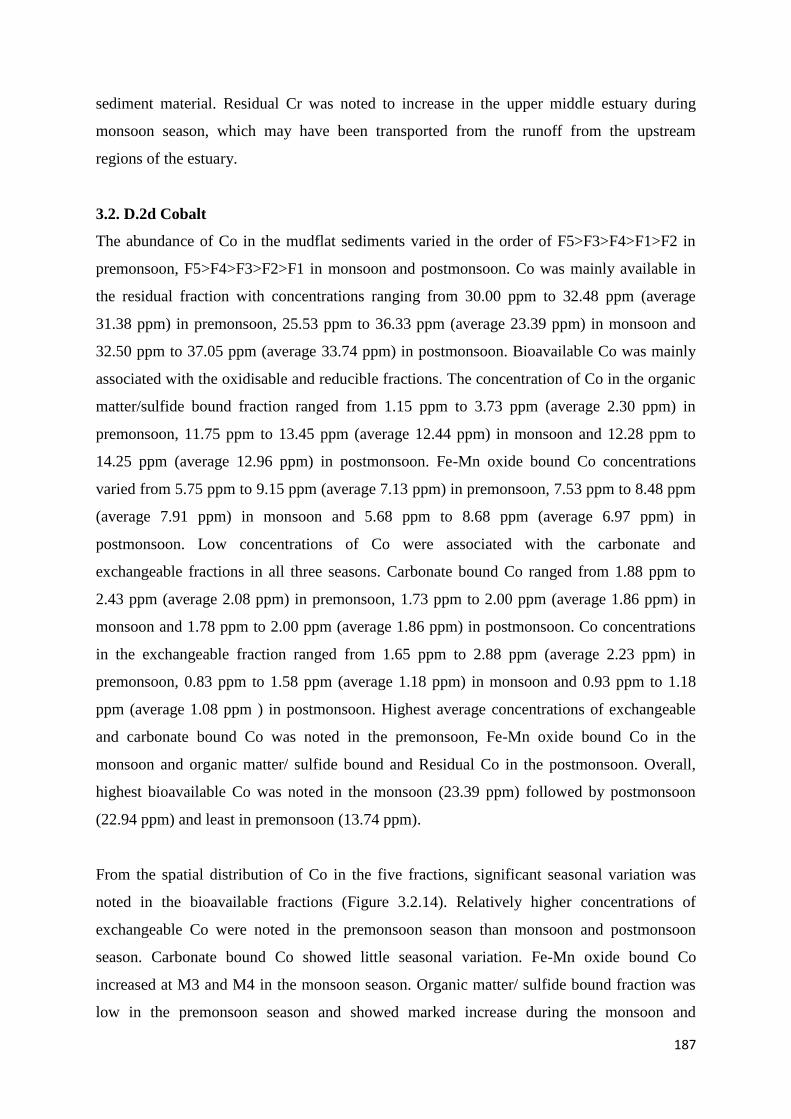
187
sediment material. Residual Cr was noted to increase in the upper middle estuary during
monsoon season, which may have been transported from the runoff from the upstream
regions of the estuary.
3.2. D.2d Cobalt
The abundance of Co in the mudflat sediments varied in the order of F5>F3>F4>F1>F2 in
premonsoon, F5>F4>F3>F2>F1 in monsoon and postmonsoon. Co was mainly available in
the residual fraction with concentrations ranging from 30.00 ppm to 32.48 ppm (average
31.38 ppm) in premonsoon, 25.53 ppm to 36.33 ppm (average 23.39 ppm) in monsoon and
32.50 ppm to 37.05 ppm (average 33.74 ppm) in postmonsoon. Bioavailable Co was mainly
associated with the oxidisable and reducible fractions. The concentration of Co in the organic
matter/sulfide bound fraction ranged from 1.15 ppm to 3.73 ppm (average 2.30 ppm) in
premonsoon, 11.75 ppm to 13.45 ppm (average 12.44 ppm) in monsoon and 12.28 ppm to
14.25 ppm (average 12.96 ppm) in postmonsoon. Fe-Mn oxide bound Co concentrations
varied from 5.75 ppm to 9.15 ppm (average 7.13 ppm) in premonsoon, 7.53 ppm to 8.48 ppm
(average 7.91 ppm) in monsoon and 5.68 ppm to 8.68 ppm (average 6.97 ppm) in
postmonsoon. Low concentrations of Co were associated with the carbonate and
exchangeable fractions in all three seasons. Carbonate bound Co ranged from 1.88 ppm to
2.43 ppm (average 2.08 ppm) in premonsoon, 1.73 ppm to 2.00 ppm (average 1.86 ppm) in
monsoon and 1.78 ppm to 2.00 ppm (average 1.86 ppm) in postmonsoon. Co concentrations
in the exchangeable fraction ranged from 1.65 ppm to 2.88 ppm (average 2.23 ppm) in
premonsoon, 0.83 ppm to 1.58 ppm (average 1.18 ppm) in monsoon and 0.93 ppm to 1.18
ppm (average 1.08 ppm ) in postmonsoon. Highest average concentrations of exchangeable
and carbonate bound Co was noted in the premonsoon, Fe-Mn oxide bound Co in the
monsoon and organic matter/ sulfide bound and Residual Co in the postmonsoon. Overall,
highest bioavailable Co was noted in the monsoon (23.39 ppm) followed by postmonsoon
(22.94 ppm) and least in premonsoon (13.74 ppm).
From the spatial distribution of Co in the five fractions, significant seasonal variation was
noted in the bioavailable fractions (Figure 3.2.14). Relatively higher concentrations of
exchangeable Co were noted in the premonsoon season than monsoon and postmonsoon
season. Carbonate bound Co showed little seasonal variation. Fe-Mn oxide bound Co
increased at M3 and M4 in the monsoon season. Organic matter/ sulfide bound fraction was
low in the premonsoon season and showed marked increase during the monsoon and

188
maintained higher concentrations during the postmonsoon. Residual concentrations also
showed significant variations with an increase in the monsoon season at M1 and decrease at
M3 and M4.
Figure 3.2.14: Spatial distribution of Co speciation in mudflat sediments in the premonsoon,
monsoon and postmonsoon.
In the premonsoon season, higher exchangeable concentrations may be attributed to
anthropogenic inputs. The decrease of exchangeable Co in the monsoon season was possibly
due to diffusion of Co to the water column from sediments and also the Co ions must have
interacted with the Fe-Mn oxides and deposited to the sediments. High organic matter bound
Co in the monsoon season was probably due to the high influx of terrestrial matter into the
estuary through runoff and the affinity of Co to humic/ fulvic substances.
3.2. D.2e Copper
The abundance of Cu in the mudflats varies in the order of F5>F4>F3>F2>F1 in
premonsoon, F5>F4>F3>F1>F2 in monsoon and F5>F4>F1>F3>F2 in postmonsoon. The
residual fraction was the dominant phase for Cu with concentrations ranging from 60.23 ppm
to 64.50 ppm (average 62.07 ppm) in premonsoon, 90.33 ppm to 222 ppm (average 135 ppm)
in monsoon and 66.30 ppm to 70.28 ppm (average 68.11 ppm) in postmonsoon. The organic
matter/ sulfide bound fraction was the major portion of the bioavailable fraction of Cu which
ranged from 5.60 ppm to 26.53 ppm (average 13.91 ppm) in premonsoon, 6.35 ppm to 54.18
ppm (average 25.62 ppm) in monsoon and 8.50 ppm to 20.10 ppm (average 14.69 ppm) in
postmonsoon. Cu in the Fe-Mn oxide bound fraction ranged from 1.45 ppm to 3.28 ppm
(average 2.11 ppm) in premonsoon and 2.58 ppm to 5.75 ppm (average 3.79 ppm) in
monsoon and 2.18 ppm to 3.13 ppm (average 2.77 ppm) in postmonsoon. Low concentration

189
of Cu was associated with the exchangeable fraction ranging from 0.28 ppm to 1.15 ppm
(average 0.77 ppm) in premonsoon, 1.23 ppm to 4.35 ppm (average 2.34 ppm) in monsoon
and 3.10 ppm to 5.05 ppm (average 3.93 ppm) in postmonsoon. Concentrations of Cu in the
carbonate bound fraction varied from 0.80 ppm to 1.65 ppm (average 1.18 ppm) in
premonsoon, 1.08 ppm to1.98 ppm (average 1.43 ppm) in monsoon and 3.10 ppm to 5.05
ppm (average 3.93 ppm) in postmonsoon,. Highest concentrations of exchangeable and
carbonate Cu were noted in the postmonsoon season whereas Fe-Mn oxide, organic matter/
sulfide bound and residual Cu were high in monsoon. Overall, bioavailable Cu concentrations
were highest during monsoon (33.18 ppm) followed by postmonsoon (22.94 ppm) and
premonsoon (17.96 ppm).
Figure 3.2.15: Spatial distribution of Cu speciation in mudflat sediments in the premonsoon,
monsoon and postmonsoon.
The spatial distribution of Cu in the three seasons indicated significant variations in the
distribution of bioavailable Cu and residual phase (Figure 3.2.15). Cu in the exchangeable,
carbonate and Fe-Mn oxide fractions maintained low concentrations in all three seasons.
However, organic matter/ sulfide bound Cu increased in the monsoon season more
prominently at stations M1 and M3 followed by decrease in postmonsoon. The residual
fraction showed significant enrichment in the monsoon season especially at station M3.
It was noted that bioavailable Cu increased in the monsoon season due to increase in the
oxidisable fraction. High organic matter influx into the estuary during the monsoon resulted
in increased binding ability of Cu to organic matter. Additionally, increased influx of
weathered material to the estuary during the monsoon led to increase in residual Cu
concentrations.

190
3.2. D.2f Zinc
The concentration of Zn in sediments varied in the order of F5>F3>F4>F2>F1 in
premonsoon, monsoon and postmonsoon seasons. Major amount of Zn was associated with
the residual fraction which ranged from 61.53 ppm to 82.33 ppm (average 70.63 ppm) in
premonsoon, 71.40 ppm to 118.45 ppm (average 91.92 ppm) in monsoon and 79.85 ppm to
84.75 ppm (average 81.92 ppm) in postmonsoon. The Fe-Mn oxide bound fraction accounted
for most quantity of the bioavailable fraction with concentrations varying from 13.85 ppm to
23.75 ppm (average 17.32 ppm) in premonsoon, 15.53 ppm to 29.33 ppm (average 20.66
ppm) in monsoon and 12.98 ppm to 15.90 ppm (average 14.38 ppm) in postmonsoon.
Considerable amount of Zn was present in the organic matter/ sulfide bound fraction ranging
from 2.98 ppm to 10.83 ppm (average 6.24 ppm) in premonsoon, 7.55 ppm to 16.30 ppm
(average 11.91 ppm) in monsoon and 6.88 ppm to 8.48 ppm (average 7.76 ppm) in
postmonsoon. Low concentration of Zn was associated with the carbonate bound and
exchangeable fractions. Zn in the carbonate bound fraction varied from 1.35 ppm to 1.80 ppm
(average 1.61 ppm) in premonsoon, 1.38 ppm to 1.98 ppm (average 1.61 ppm) in monsoon
and 1.23 ppm to 3.45 ppm (average 2.48 ppm) in postmonsoon. Least concentrations of Zn
were found in the exchangeable fraction and ranged from 0.43 ppm to 1.80 ppm (average
1.22 ppm) in premonsoon, 0.68 ppm to 1.13 ppm (average 0.85 ppm) in monsoon and 0.95
ppm to 1.58 ppm (average 1.23 ppm) in postmonsoon. Highest Zn concentrations for
exchangeable and carbonate bound Zn were noted in postmonsoon and Fe-Mn oxide, organic
matter/ sulfide bound and residual Zn in monsoon season. Overall, the sediments had higher
concentration of Zn in the monsoon season (average 35.03 ppm) followed by premonsoon
(26.38 ppm) and postmonsoon (25.85 ppm).
Figure 3.2.16: Spatial distribution of Zn speciation in mudflat sediments in the premonsoon,
monsoon and postmonsoon.
191
The spatial distribution of Zn exhibited low concentrations for exchangeable and carbonate
bound fraction in all the three seasons (Figure 3.2.16). Fe-Mn oxide bound Zn showed minor
enrichment in the monsoon season. Significant increase was also noted for organic matter /
sulfide bound Zn in monsoon season at all three mudflat locations. The residual fraction of
Zn showed marked increase in monsoon season more prominently at M1 and M3. This
variation was due to the large influx of terrestrial matter in the estuary that aided in binding
of metals.
From the results described above, it was noted that the bioavailable concentration of metals in
mangroves (Fe, Mn, Co, Cu and Zn) and mudflats (Fe, Co, Cu and Zn) was high during the
monsoon season. However, most residual metals showed enrichment in the postmonsoon
season for mangroves (Fe, Mn, Cr, Co and Zn) as well as mudflats (Fe, Mn, Cr and Co).
Among the bioavailable fractions of metals in the surface sediments, most seasonal variations
was observed in the Fe-Mn oxide bound and organic/sulfide bound fractions. A seasonal
effect is apparent mainly for Mn and Co, which show large similarity and thus may be related
to the same anthropogenic source.
The Zuari estuary is affected by several human activities such as mining, boating barge/
shipbuilding and land reclamation etc. through which considerable amount of material is
added to the estuary overtime. In addition, high rainfall in the Western Ghats leads to active
drainage, permitting strong to very strong hydrolytic action on parent rocks (Kessarkar et al.,
2013) which wash off into the tributaries of river and estuary. Mining and associated
industries also elevate the level of metals in the estuary.
An increase in the concentrations of few metals in the sediments during premonsoon and
post-monsoon periods indicated that these metals were mobilized from the over-flooding of
metal rich wastewater into the estuary during high rainfall and by reworking of the sediments
(Ansari et al., 2000). Further, geochemical processes facilitated the metal dispersion and
mobilization in estuarine sediments after, large-scale sediment-water movement during the
monsoon period. In monsoon, the metals released by from the basin, mining effluents, and
other anthropogenic sources, are drained into the Zuari estuary mainly through surface and
subsurface discharges increasing bioavailable metal concentrations. Heavy rainfall during the
monsoon would have flushed Fe–Mn oxides stored on the surface, associated with some

192
transition metals Co, Ni, Cu, Zn in particular (Kabata-Pendias and Pendias, 2001) and the
Fe–Mn oxides along with their leachates transported to the estuary (Kessarkar et al., 2013).
Further, in postmonsoon, the subsurface discharge might have contributed substantial detrital
metals to the estuary. In Goa, 52% of monsoon rainfall accounts for the surface runoff while
16 % accounts for charging the ground water (Ghosh, 1985). The ground water discharges
into estuary from the laterites, that contain water reservoirs in them and sustain several
springs, could be significant in the non-monsoon seasons (Chachadi, 2009; Anand et al.,
2014). Subramaniam (1981) found that the effluence of the leaky laterites sustains the high
discharges from rivers and tributaries, all along their course, especially in postmonsoon
season. Additionally, discharges of fresh water from the Selaulim dam in the upstream region
and subsurface flow contributes to the Zuari estuarine system in dry seasons (Shetye et al.,
2007, Subramaniam, 1981). Thus, the ground water from the lateritic rocks could add
minerals resulting in higher residual bound metals to the estuary in the postmonsoon season.
Moreover, geomorphology and drainage type combined with sedimentation processes played
a substantial role on distribution of metals bound to sediments. Therefore, the monsoon
hydrography and physico-chemical parameters of the estuary play a major role in regulating
the concentrations and behavior of the metals in the estuarine system.
3.2. E Risk assessment
The average bioavailable concentrations of metals Fe, Mn, Cr, Co, Cu and Zn (Table 3.2.5)
were compared with the Sediment quality values of the SQuiRT proposed by Buchman
(1999).
Table 3.2.5: Concentrations of metals in the bioavailable fraction of mangrove and mudflat
sediments expressed in ppm (except for Fe, which is expressed in percentage)
Fe Mn Cr Co Cu Zn
(a) Mangrove Premonsoon 0.75 2845(>AET) 30.77 12.53(>AET) 15.44 25.95
Monsoon 0.75 3493(>AET) 23.45 22.88(>AET) 26.76(>TEL) 34.5
Postmonsoon 0.58 3431(>AET) 23.15 21.99(>AET) 21.59(>TEL) 28.02
(b) Mudflats Premonsoon 0.68 3830(>AET) 33.12 13.74(>AET) 17.96 26.38
Monsoon 0.87 3042(>AET) 24.56 23.39(>AET) 33.18(>TEL) 35.03
Postmonsoon 0.55 3750(>AET) 23.68 22.94(>AET) 22.94(>TEL) 25.85

193
In the mangroves and mudflat sediments, bioavailable Mn and Co concentrations were higher
than the Apparent Effects Threshold in all three seasons and can cause adverse effects on
biota, whereas bioavailable concentrations of Cu in monsoon and postmonsoon were greater
than the Threshold Effect Level and can pose considerable risk to biota. Moreover, higher
concentrations during monsoon can cause significant toxicity to the sediment dwelling
organisms.
Table 3.2.6: Risk assessment code calculated form Mangrove and mudflat sediments with
reference to the labile fraction (exchangeable +carbonate) expressed in percentage.
Fe Mn Cr Co Cu Zn
(a) Mangroves Premonsoon 0.07 38.90 1.45 7.02 2.45 2.75
Monsoon 0.05 32.15 0.445 6.07 3.35 2.21
Postmonsoon 0.10 24.55 0.59 4.81 5.84 3.02
(b) Mudflats Premonsoon 0.10 33.74 1.55 9.58 2.37 2.90
Monsoon 0.02 34.47 0.49 5.86 2.53 2.03
Postmonsoon 0.05 23.61 0.53 5.35 6.00 3.44
The Risk assessment code calculated for the metals in the mangrove and mudflat sediments
(Table 3.2.6) revealed that concentrations of labile Mn (exchangeable + carbonate) posed
high risk in the premonsoon and monsoon seasons and medium risk in the postmonsoon
season. The decrease in labile Mn in postmonsoon was probably due to dilution by seawater
with higher salinity and conversion of labile Mn to oxide form.

194
3.3 Sediment collection in premonsoon of 2015, after mining ban
Sediment cores of 10 cm each were collected in the premonsoon season of 2015 to evaluate
the concentration of metals in sediments following the mining ban imposed in 2012 to
understand the changes in bioavailability. Further, efforts were made to assess the
bioaccumulation of metals in mangrove pneumatophores and sediment associated biota
relative to the bulk, bioavailable and labile metal content in sediments of the Zuari estuary.
Four mangrove (S1, S2, S3 and S4) and three mudflat (M1, M2 and M4) cores collected were
analyzed at 2 cm interval and the average data was considered for data interpretations. The
sediments were analyzed for pH, sediment component, organic carbon, bulk metals and metal
concentration in various sediment fractions.
3. 3.A Mangroves
3.3. A.1 Sediment components
The range and average values of sediment components are presented in table 3.3.1(a).
The data revealed that the pH values recorded varied between 6 and 7. Near neutral pH was
noted in the lower estuarine sediments whereas the sediments towards the upstream regions
of the estuary and the Cumbharjua canal were weakly acidic in nature. The sediments of the
estuarine mangroves were characterized by the fine size. Higher clay was noted in the upper
middle estuary (80 %) which decreased towards the lower estuary (48 % at station S4) due to
changes in hydrodynamics. Highest silt percentage was noted in the Cumbharjua canal (28.53
%) and sand in the lower estuary (27.96 %). The lower estuary is subjected to high
hydrodynamics due to turbulence by waves causing resuspension of the finer sediments
which are carried in suspension thus retaining the larger sediment size fractions at the lower
estuary. High total organic carbon (TOC) content was noted in the lower middle estuarine
(4.67 %) sediments. Organic matter is supplied to the estuarine environments from both
external (terrestrial, domestic and municipal sewage) and internal (algal and microbial mats)
sources. Benthic invertebrates and soil microorganisms may also contribute significant
amounts of organic carbon to sediments (Reddy and DeLaune, 2008).
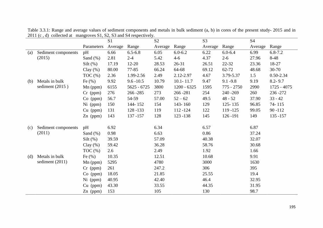
195
Table 3.3.1: Range and average values of sediment components and metals in bulk sediment (a, b) in cores of the present study- 2015 and in
2011 (c , d) collected at mangroves S1, S2, S3 and S4 respectively.
S1 S2 S3 S4
Parameters Average Range Average Range Average Range Average Range
(a) Sediment components
(2015)
pH 6.66 6.5-6.8 6.05 6.0-6.2 6.22 6.0-6.4 6.99 6.8-7.2
Sand (%) 2.81 2-4 5.42 4-6 4.37 2-6 27.96 8-48
Silt (%) 17.19 12-20 28.53 26-31 26.51 22-32 23.36 18-27
Clay (%) 80.00 77-85 66.24 64-68 69.12 62-72 48.68 30-70
TOC (%) 2.36 1.99-2.56 2.49 2.12-2.97 4.67 3.79-5.37 1.5 0.50-2.34
(b) Metals in bulk
sediment (2015 )
Fe (%) 9.92 9.6 -10.5 10.79 10.1- 11.7 9.47 9.1 -9.8 9.19 8.2- 9.7
Mn (ppm) 6155 5625 - 6725 3800 1200 - 6325 1595 775 - 2750 2990 1725 - 4075
Cr (ppm) 276 266 -285 273 266 -281 254 240 -269 260 236 -272
Co (ppm) 56.7 54-59 57.00 52 – 62 49.5 48 - 52 37.90 33 - 42
Ni (ppm) 150 144- 152 154 143- 160 129 125- 135 96.85 74- 115
Cu (ppm) 131 128 -133 119 112 -124 122 119 -125 99.05 90 -112
Zn (ppm) 143 137 -157 128 123 -138 145 126 -191 149 135 -157
(c) Sediment components
(2011)
pH 6.92 6.34 6.57 6.87
Sand (%) 0.98 6.63 0.86 37.24
Silt (%) 39.59 57.09 40.38 32.07
Clay (%) 59.42 36.28 58.76 30.68
TOC (%) 2.6 2.49 1.92 1.66
(d) Metals in bulk
sediment (2011)
Fe (%) 10.35 12.51 10.68 9.91
Mn (ppm) 5295 4780 3000 1630
Cr (ppm) 261 247.2 306 395
Co (ppm) 18.05 21.85 25.55 19.4
Ni (ppm) 40.95 42.40 46.4 32.95
Cu (ppm) 43.30 33.55 44.35 31.95
Zn (ppm) 153 105 130 98.7

196
3.3. A.2 Geochemistry of metals
The range and average values of metals Fe, Mn, Cr, Co, Ni, Cu and Zn in bulk sediments are
presented in table 3.3.1(b).
Substantial spatial variations were noted in the distribution of metals. Highest average
concentrations of Fe, Co and Ni were noted in the Cumbharjua canal, followed by the upper
middle estuary which progressively decreased towards the lower estuary. Mn, Cr, and Cu were
enriched in the upper middle estuary and Zn in the lower estuary. The distribution of Co and Ni
in the Cumbharjua canal sediments may have been influenced by Fe oxyhydroxides and silt. The
enrichment of Cr and Cu in the upper middle estuary may have been influenced by Mn
oxyhydroxides and clay. Zn enrichment in the lower estuary may have been influence by pH of
the sediments
A comparison of the average values of sediment components and metal concentrations was
attempted with the data of mangrove sediments collected in the year 2011 of the upper 10 cm of
the cores at the same sampling locations before the mining ban was imposed (Table 3.3.1 c and
d). It was observed that the silt fraction of the sediments at all the locations has considerably
decreased which was compensated by an increase in the clay fraction. The trace metals
concentrations have significantly increased in recent times. Mn, Cr, Co, Ni and Cu showed
higher values at site S1; Cr, Co, Ni, Cu and Zn in core S2; Co, Ni, Cu and Zn at S3, and Mn, Co,
Ni, Cu and Zn at S4. However, Fe concentrations at all sampling locations were lower as
compared to 2011.
Table 3.3.2: Paired-samples t-test for the comparison of means of sediment components and
metals in cores S1, S2, S3 and S4 with respect to year 2011before mining ban and 2015 after
mining ban.
Pairs of variables
Difference of
means T df Sig. (2-tailed)
S1 Sand2011 - Sand2015 -1.82 -3.49 4.00 0.03
Silt2011 - Silt2015 22.40 9.15 4.00 0.00
Clay2011 - Clay2015 -20.58 -9.11 4.00 0.00
TOC2011 - TOC2015 0.23 2.16 4.00 0.10
Fe2011 - Fe2015 0.43 1.54 4.00 0.20
Mn2011 - Mn2015 -860 -2.37 4.00 0.08
Cr2011 - Cr2015 -15.05 -2.53 4.00 0.06
Co2011 - Co2015 -38.65 -15.26 4.00 0.00
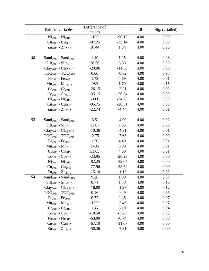
197
Pairs of variables
Difference of
means T df Sig. (2-tailed)
Ni2011 - Ni2015 -109 -90.13 4.00 0.00
Cu2011 - Cu2015 -87.25 -32.14 4.00 0.00
Zn2011 - Zn2015 10.44 1.34 4.00 0.25
S2 Sand2011 - Sand2015 1.40 1.25 4.00 0.28
Silt2011 - Silt2015 28.56 8.53 4.00 0.00
Clay2011 - Clay2015 -29.96 -11.36 4.00 0.00
TOC2011 - TOC2015 0.00 -0.02 4.00 0.98
Fe2011 - Fe2015 1.72 4.69 4.00 0.01
Mn2011 - Mn2015 980 1.79 4.00 0.15
Cr2011 - Cr2015 -26.15 -2.21 4.00 0.09
Co2011 - Co2015 -35.15 -26.54 4.00 0.00
Ni2011 - Ni2015 -111 -24.26 4.00 0.00
Cu2011 - Cu2015 -85.75 -28.31 4.00 0.00
Zn2011 - Zn2015 -22.74 -4.44 4.00 0.01
S3 Sand2011 - Sand2015 -3.51 -4.00 4.00 0.02
Silt2011 - Silt2015 13.87 7.85 4.00 0.00
Clay2011 - Clay2015 -10.36 -4.81 4.00 0.01
TOC2011 - TOC2015 -2.75 -7.63 4.00 0.00
Fe2011 - Fe2015 1.20 4.40 4.00 0.01
Mn2011 - Mn2015 1405 5.08 4.00 0.01
Cr2011 - Cr2015 51.65 4.60 4.00 0.01
Co2011 - Co2015 -23.95 -26.23 4.00 0.00
Ni2011 - Ni2015 -82.25 -32.05 4.00 0.00
Cu2011 - Cu2015 -77.90 -58.72 4.00 0.00
Zn2011 - Zn2015 -15.10 -1.13 4.00 0.32
S4 Sand2011 - Sand2015 9.28 1.00 4.00 0.37
Silt2011 - Silt2015 8.71 1.70 4.00 0.16
Clay2011 - Clay2015 -18.00 -1.97 4.00 0.12
TOC2011 - TOC2015 0.16 0.49 4.00 0.65
Fe2011 - Fe2015 0.72 2.45 4.00 0.07
Mn2011 - Mn2015 -1360 -2.46 4.00 0.07
Cr2011 - Cr2015 135 3.10 4.00 0.04
Co2011 - Co2015 -18.50 -3.26 4.00 0.03
Ni2011 - Ni2015 -63.90 -6.74 4.00 0.00
Cu2011 - Cu2015 -67.10 -11.07 4.00 0.00
Zn2011 - Zn2015 -50.36 -7.81 4.00 0.00

198
The paired sample t-test (Table 3.3.2) conducted on the means of the four cores with respect to
the years 2011 and 2015, support the observations made in table 3.3.1 (c and d), with
significantly higher mean values of trace metal concentrations in 2015 indicated by negative t-
values. Positive t-values of Fe indicated higher mean values in the year 2011 before mining ban,
which decreased in the year 2015. The decrease in Fe content may be due to the reduced input
from iron ore mining activities and transportation from the catchment area of the Zuari. Positive t
values were also obtained for silt at all the locations. It was reported previously that Iron was
associated with the larger grain sized sediments such as magnetic iron minerals in the Mandovi-
Zuari estuarine system (Dessai et al., 2009; Veerasingam et al., 2015; Noronha-D’Mello and
Nayak, 2015). The increase in trace metal concentrations may be due to the increase in the clay
fraction, which has a higher adsorption capacity than the larger grain size fractions. In the recent
years, sand mining has increased in the Zuari estuary, which caused resuspension and settling of
the fine sediments with time. This must have helped in remobilization of trace metals, which
later deposited in the calm mangrove sediments. Additionally, discharges from ship building
industries and sewage release on the shores of the Zuari River may have also contributed to the
enhancement of trace metal concentrations in the Zuari estuary. Kessarkar et al. (2013), however,
suggested that suspended particulate matter from fluvial sources could be the dominant source of
trace metals in the Zuari estuary.
3.3. B Mudflats
The distribution of various sediment components and metals in the three sediments cores M1,
M3 and M4 of 10 cm each collected in 2015 from mudflats of the Zuari estuary are presented
below.
3.3. B.1 Sediment components
The range and average values of the sediment components in mudflat sediments is presented in
table 3.3.3 (a). The results revealed that the mudflat sediments were characterized by near neutral
pH and high mud fraction. The dominant grain size fraction was clay and was high in the lower
middle estuary (73.12 %), followed by silt that was abundant in the upper middle estuary (31.19
%) and least was sand that showed higher percentage in the lower estuary (6.63 %). The presence
of coarser sediments in the lower estuary indicated strong hydrodynamic conditions operated in

199
the area whereas higher finer sediments in the middle estuary indicated calmer depositional
conditions. TOC was abundant in the upper middle estuary (2.41 %) among the mudflats and
was associated with the higher silt content. The lower estuary is known for higher wave and tidal
dynamics that is responsible for facilitating the deposition of coarser sediments (Chen, 1992) and
carrying finer sediments towards the middle estuary during the flood tide.
3.3. B.2 Geochemistry of metals
The distribution of metals in the mudflat sediments exhibited considerable spatial variations.
From table 3.3.3(b), Mn, Co and Ni showed high concentrations in the upper middle estuary, Cr
and Cu were enriched in the lower middle estuarine sediments, and Fe and Zn showed high
concentrations in the lower estuary. The high silt and TOC content in the upper middle estuary
mudflat along with the high Mn content may have influenced the enrichment of Co and Ni. The
enrichment of Cr and Cu in the sediments of the lower middle estuarine mudflat might have
influenced by the high clay content. Further, the enrichment of Zn in the lower estuary can be
attributed to the high Fe content in the sediments along with pH and to some extent the sand
content.
A comparison of average values of sediment components and metal concentration of 2011 and
2015 datasets revealed that the concentrations of trace metals along with clay in the estuarine
sediments had considerably increased whereas Fe concentration along with silt and organic
matter had decreased (Table 3.3.3). In core M1, metal concentrations of Mn, Cr, Co, Ni, Cu and
Zn along with sand, clay were higher in 2015 as compared to 2011 whereas Fe along with silt
and TOC were higher in 2011. In core M3, Co Ni, Cu and Zn concentrations along with sand and
clay were higher in 2015 whereas Fe, Mn and Cr along with silt and TOC showed higher average
values in 2011. In core M4, Fe, Mn, Co Ni, Cu, Zn and clay were higher in 2015 whereas Cr,
sand, silt and TOC were higher in 2011.
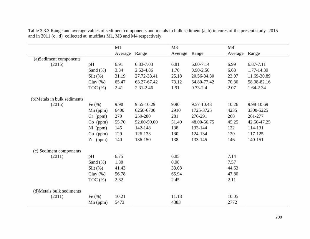
200
Table 3.3.3 Range and average values of sediment components and metals in bulk sediment (a, b) in cores of the present study- 2015
and in 2011 (c , d) collected at mudflats M1, M3 and M4 respectively.
M1 M3 M4
Average Range Average Range Average Range
(a)Sediment components
(2015) pH 6.91 6.83-7.03 6.81 6.60-7.14 6.99 6.87-7.11
Sand (%) 3.34 2.52-4.86 1.70 0.90-2.50 6.63 1.77-14.39
Silt (%) 31.19 27.72-33.41 25.18 20.56-34.30 23.07 11.69-30.89
Clay (%) 65.47 63.27-67.42 73.12 64.80-77.42 70.30 58.08-82.16
TOC (%) 2.41 2.31-2.46 1.91 0.73-2.4 2.07 1.64-2.34
(b)Metals in bulk sediments
(2015) Fe (%) 9.90 9.55-10.29 9.90 9.57-10.43 10.26 9.98-10.69
Mn (ppm) 6400 6250-6700 2910 1725-3725 4235 3300-5225
Cr (ppm) 270 259-280 281 276-291 268 261-277
Co (ppm) 55.70 52.00-59.00 51.40 48.00-56.75 45.25 42.50-47.25
Ni (ppm) 145 142-148 138 133-144 122 114-131
Cu (ppm) 129 126-133 130 124-134 120 117-125
Zn (ppm) 140 136-150 138 133-145 146 140-151
(c) Sediment components
(2011) pH 6.75
6.85
7.14
Sand (%) 1.80
0.98
7.57
Silt (%) 41.43
33.08
44.63
Clay (%) 56.78
65.94
47.80
TOC (%) 2.82
2.45
2.11
(d)Metals bulk sediments
(2011) Fe (%) 10.21
11.18
10.05
Mn (ppm) 5473
4383
2772

201
Cr (ppm) 264
371
342
Co (ppm) 32.10
21.90
28.45
Ni (ppm) 44.40
43.30
42.35
Cu (ppm) 47.95
40.95
40.65
Zn (ppm) 136
133
128
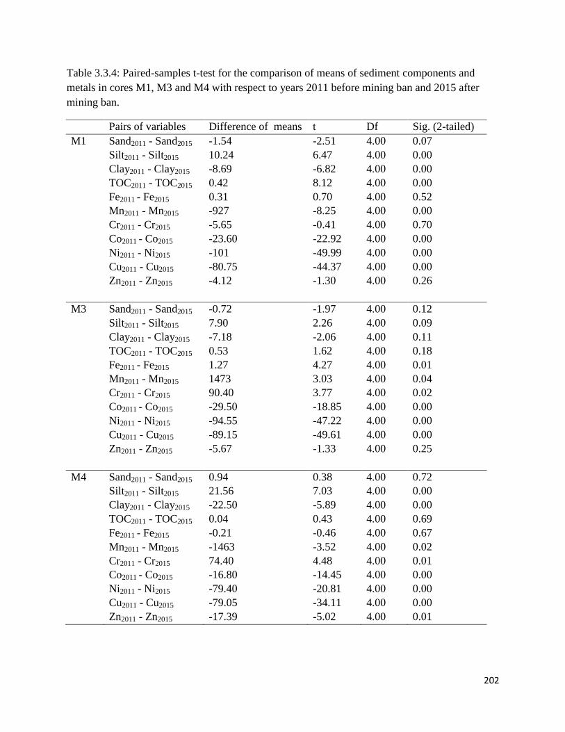
202
Table 3.3.4: Paired-samples t-test for the comparison of means of sediment components and
metals in cores M1, M3 and M4 with respect to years 2011 before mining ban and 2015 after
mining ban.
Pairs of variables Difference of means t Df Sig. (2-tailed)
M1 Sand2011 - Sand2015 -1.54 -2.51 4.00 0.07
Silt2011 - Silt2015 10.24 6.47 4.00 0.00
Clay2011 - Clay2015 -8.69 -6.82 4.00 0.00
TOC2011 - TOC2015 0.42 8.12 4.00 0.00
Fe2011 - Fe2015 0.31 0.70 4.00 0.52
Mn2011 - Mn2015 -927 -8.25 4.00 0.00
Cr2011 - Cr2015 -5.65 -0.41 4.00 0.70
Co2011 - Co2015 -23.60 -22.92 4.00 0.00
Ni2011 - Ni2015 -101 -49.99 4.00 0.00
Cu2011 - Cu2015 -80.75 -44.37 4.00 0.00
Zn2011 - Zn2015 -4.12 -1.30 4.00 0.26
M3 Sand2011 - Sand2015 -0.72 -1.97 4.00 0.12
Silt2011 - Silt2015 7.90 2.26 4.00 0.09
Clay2011 - Clay2015 -7.18 -2.06 4.00 0.11
TOC2011 - TOC2015 0.53 1.62 4.00 0.18
Fe2011 - Fe2015 1.27 4.27 4.00 0.01
Mn2011 - Mn2015 1473 3.03 4.00 0.04
Cr2011 - Cr2015 90.40 3.77 4.00 0.02
Co2011 - Co2015 -29.50 -18.85 4.00 0.00
Ni2011 - Ni2015 -94.55 -47.22 4.00 0.00
Cu2011 - Cu2015 -89.15 -49.61 4.00 0.00
Zn2011 - Zn2015 -5.67 -1.33 4.00 0.25
M4 Sand2011 - Sand2015 0.94 0.38 4.00 0.72
Silt2011 - Silt2015 21.56 7.03 4.00 0.00
Clay2011 - Clay2015 -22.50 -5.89 4.00 0.00
TOC2011 - TOC2015 0.04 0.43 4.00 0.69
Fe2011 - Fe2015 -0.21 -0.46 4.00 0.67
Mn2011 - Mn2015 -1463 -3.52 4.00 0.02
Cr2011 - Cr2015 74.40 4.48 4.00 0.01
Co2011 - Co2015 -16.80 -14.45 4.00 0.00
Ni2011 - Ni2015 -79.40 -20.81 4.00 0.00
Cu2011 - Cu2015 -79.05 -34.11 4.00 0.00
Zn2011 - Zn2015 -17.39 -5.02 4.00 0.01

203
Furthermore, the observations of the compared average values was supported by the results of
the paired sample t-test where negative t-values of the variables indicated increase in trace metal
concentrations in recent times and positive t-values indicated a significant decrease (Table 3.3.4).
The increase in trace metals in the estuary may be related to sand mining operations that might
have re-suspended the sediments causing the metals to interact with suspended matter and clay
and were re-deposited to sediments. Additionally, anthropogenic inputs and their deposition to
the sediments was facilitated by adsorption onto clay particles or formation of coating on sand
particles. However, a significant decrease in Fe and silt (M1 and M3) indicated reduction in Fe
inputs to the estuary in recent times.
3.3.C Geoaccumulation index
3.3.C.1 Mangroves
Table 3.3.5: Geoaccumulation index of metals in sediments of core mangrove S1, S2, S3 and S4.
Fe Mn Cr Co Ni Cu Zn
S1 0.49 2.27 1.03 0.99 0.74 0.95 0.00
S2 0.61 1.40 1.02 1.00 0.77 0.82 -0.16
S3 0.42 0.19 0.91 0.80 0.51 0.86 0.00
S4 0.37 1.16 0.95 0.40 0.09 0.55 0.06
Geo-accumulation index (Muller, 1979) was computed to assess the level of metal contamination
of sediments (Table 3.3.5). There was significant contamination of Mn and Cr in the estuary
which varied spatially. Overall, higher Igeo values for all metals except for Zn were noted in the
upper middle estuary and Cumbharjua canal. On comparing Igeo values with earlier study based
on collection in 2011 (Noronha-D’Mello and Nayak, 2015), mangrove sediments that were
previously significantly polluted by Fe, Mn and Cr in 2011 showed lower index for Fe in the
present study and Igeo values of Mn increased at locations S1 and S4 and decreased at S2 and
S3. Igeo values of Cr were similar to previously reported values at S1 and S2, however, Igeo
values decreased at locations S3 and S4 than previously reported. This indicated that there was a
substantial reduction of Fe and Cr inputs to the Zuari estuary due to ban on mining in the
catchment area.

204
3.3. C.2 Mudflats
Table 3.3.6: Geoaccumulation index of metals in sediments of core mudflat M1, M3 and M4.
Fe Mn Cr Co Ni Cu Zn
M1 0.48 2.33 1.00 0.96 0.69 0.93 -0.03
M3 0.48 1.14 1.06 0.85 0.61 0.95 -0.05
M4 0.53 1.70 0.99 0.67 0.43 0.83 0.03
The Geoaccumulation index of mudflat sediments revealed that there was significant amount of
Mn and Cr in the sediments (Table 3.3.6). On comparing with the Igeo values of mudflat
sediments collected in the premonsoon season of 2011, Igeo values of Fe at the three mudflat
stations decreased after the imposition of the mining ban. Igeo values of Mn at M1 and M4
increased whereas Mn at M3 decreased in recent times. Igeo value of Cr at M1 increased
whereas at M3 and M4 it decreased in recent times. The Igeo values of Co, Ni, Cu and Zn
increased after the imposition of the mining ban. Thus, there was considerable remobilization of
Mn, Co, Ni, Cu and Zn in the sediments in recent times due increased human activities like sand
mining. Additionally, enhanced anthropogenic input in recent years must have contributed to the
increase of index.
3.3.D Speciation of metals
3.3.D.1 Mangroves
The average values of bioavailability of metals in the sediments carried out through sequential
extraction within the five geochemical phases viz. exchangeable (F1), Carbonate (F2), Fe-Mn
oxide/reducible (F3), organic matter and sulfide bound/ oxidisable (F4) and residual (F5) for
cores S1, S2, S3 and S4 in the present study (a) and 2011 (b) are presented in table 3.3.7.
The metal data collected in the pre-mining ban period (2011) was compared with the post mining
ban period (2015) using the isocon diagram for each of the analyzed metals and is illustrated in
figure 3.3.1.

205
Table 3.3.7 Concentration of metals in various sediment fractions, bioavailable and Labile
(Exchangeable + carbonate) fractions of mangrove cores S1, S2, S3 and S4 in present study 2015
(a) and 2011 (b).
(a) Exchangeable Carbonate Fe-Mn
oxide
Organic
matter/
Sulfide
Residual Sum of
Bioavailable
fractions
Exchangeable
+ Carbonate
(ppm) (ppm) (ppm) (ppm) (ppm) (ppm) (%) (ppm)
Fe S1 3.56 10.91 6053 3170 83805 9236 0.02 14.47
S2 4.86 15.48 5464
.00
2368 95122 7852 0.02 20.34
S3 3.22 34.34 4537 7990 69751 12564 0.05 37.56
S4 1.99 17.55 5623 1089 77083 6732 0.02 19.54
Mn S1 518 1849 2838 489 557 5696 37.97 2369
S2 590 765 1592 218 499 3165 35.09 1355
S3 371 345 313 66.00 329 1094 50.33 715
S4 158 1025 1047 107 614 2337 39.41 1183
Cr S1 7.79 0.94 8.26 14.73 305 31.71 2.59 8.73
S2 5.53 2.42 11.14 21.06 301 40.13 2.32 7.95
S3 8.75 0.91 8.40 12.39 213 30.45 4.08 9.66
S4 7.92 3.00 6.26 16.23 248 33.41 3.88 10.92
Co S1 1.72 4.02 8.87 4.71 40.20 19.31 9.64 5.74
S2 2.05 3.15 9.20 4.22 37.99 18.61 9.17 5.20
S3 2.69 4.19 6.21 5.34 40.56 18.42 11.69 6.88
S4 0.86 3.73 6.09 2.69 36.97 13.36 9.10 4.59
Ni S1 0.79 1.63 8.59 7.91 96.77 18.91 2.08 2.42
S2 1.92 1.70 10.43 7.90 92.59 21.95 3.16 3.62
S3 1.96 1.80 7.08 8.52 85.25 19.35 3.64 3.76
S4 1.81 1.94 6.58 3.52 76.28 13.84 4.21 3.75
Cu S1 3.67 1.07 1.38 16.29 65.64
22.40 5.38 4.74
S2 3.67 0.43 1.39 15.84 57.21 21.32 5.20 4.10
S3 6.39 0.36 0.37 22.45 55.58 29.57 7.91 6.75
S4 0.19 1.58 1.30 9.57 73.11 12.63 2.08 1.77
Zn S1 5.38 3.32 24.03 14.06 107 46.78 5.68 8.70
S2 5.12 1.88 16.63 10.55 83.35 34.17 5.97 7.00
S3 6.69 3.50 21.63 17.05 87.13 48.86 7.60 10.19
S4 2.87 4.12 30.28 9.20 103 46.46 4.68 6.99

206
(b) Core Exchangeable Carbonate Fe-Mn
oxide
Organic/Sulfide Residual Bioavailable
Fraction
(ppm) (ppm) (ppm) (ppm) (ppm) (ppm)
Fe S1 15.84 5.69 7921 902 76452 8844
S2 14.88 3.50 8326 1280 89240 9624
S3 64.51 5.03 5650 955 77690 6674
S4 76.68 7.38 3887 184 62464 4154
Mn S1 562 1945 2362 268 485 5136
S2 609 717 2717 228 612 4270
S3 338 666 984 248 516 2235
S4 130 350 411 174 471 1064
Cr S1 1.62 0.91 11.43 13.27 198 27.22
S2 0.87 1.37 10.86 11.26 169 24.35
S3 2.16 0.95 11.54 24.07 177 38.70
S4 1.38 1.49 10.99 14.27 177 28.12
Co S1 1.00 1.32 9.71 3.16 34.19 15.19
S2 1.27 1.19 11.51 2.19 27.12 16.16
S3 2.14 1.21 5.89 2.31 33.93 11.55
S4 1.32 2.25 4.77 1.20 27.37 9.54
Cu S1 1.30 1.56 2.91 21.82 82.52 27.59
S2 1.13 1.11 2.06 11.27 69.12 15.56
S3 0.88 0.83 1.23 10.34 56.39 13.28
S4 1.36 1.21 0.74 4.38 44.24 7.68
Zn S1 0.67 1.95 22.06 9.75 80.95 34.42
S2 0.87 1.56 15.24 6.72 69.00 24.38
S3 1.22 2.18 14.66 5.87 87.08 23.93
S4 6.23 1.54 12.78 2.80 57.82 23.35
Iron was mainly associated with the residual fraction of sediments at all the four studied sites of
the estuary (69751 ppm to 95122 ppm) which accounted to 85% to 92 %. Fe in the bioavailable
fractions (F1+F2+F3+F4) was low in all cores. On comparing bioavailability of Fe in the post
mining ban period (2015) with pre-mining ban (2011) Fe in the exchangeable fraction decreased
at all stations and Fe-Mn oxide decreased at stations S1, S2 and S3 in the post mining ban period
(Figure 3.3.1). Considerable increase of Fe in organic/sulfide bound and carbonate fraction was

207
noted in the present study as compared to 2011. Increased Fe in the organic/sulfide phase in
recent times suggested the association of Fe with organic matter and/or sulfides probably in the
absence of fresh Fe input from mining. Also, organic matter decay by microorganisms must have
facilitated Fe immobilization.
Cr in the Zuari estuary was mainly associated with the residual phase (213 ppm to 385 ppm) that
accounted to 87 % to 91 %. Highest bioavailable Cr concentrations was noted in core S2
followed by S4, S1 and S3. Bioavailable concentrations of Cr at S1, S2, and S4 were higher in
the post-mining ban period than pre-mining ban (Figure 3.3.1). The increase in bioavailable
concentrations at S1, S2 and S4 was due to increase of exchangeable, organic matter and
carbonate bound Cr.
Considerable amount of Co was associated with the residual phase as compared to other phases
(36.97 ppm to 40.56 ppm that accounted to 67 % to 73 %) with considerable quantity in
bioavailable phases. Most bioavailable Co concentration was noted in sediments of S1 followed
by S2, S3, and S4 and was mainly associated with the Fe-Mn oxide phase. Comparison of
bioavailability of Co in the pre-mining ban with the present results showed that Co
bioavailability had significantly increased in recent times due to increase in organic bound,
carbonate, and exchangeable fractions.
Ni in the Zuari estuary was also largely associated with residual fraction (76.28 ppm to 96.77
ppm that accounted to 81 % to 85 %) that consists essentially of detrital silicate minerals.
Highest average concentration of bioavailable Ni was noted at S2 followed by S3, S1 and S4 and
was mainly associated with the Fe-Mn oxide bound and organic matter/ sulfide bound phases.
Cu was also mainly associated with the residual phase (55.58 ppm to 73.11 ppm that accounted
to 65% to 85 %) in the Zuari estuary with considerable quantity in the bioavailable phases.
Higher average bioavailable Cu concentration was noted in S3 followed by S1, S2 and S4 with
high concentrations in the organic matter/sulfide bound phase. The bioavailability of Cu
increased in recent times at S2, S3, and S4 when compared with pre-mining ban results mainly
due to the increase in the organic bound and exchangeable fractions.

208
Figure 3.3.1 : Isocon
diagram of Fe, Mn,
Cr, Co, Cu and Zn in
the exchangeable
(F1), Carbonate
(F2), Fe-Mn oxide
bound (F3), Organic
matter/ sulfide
bound (F4),
Residual (F5) and
total bioavailable
(B) fraction of
sediments of cores
S1, S2, S3 and S4 in
2011 and 2015.

209
Much of the Zn was associated with the residual phase of the sediments (83.35 ppm to 107 ppm
that accounted to 64 % to 71 %) with considerable quantity in the bioavailable phases. The
bioavailability of Zn had considerably increased in recent times when compared with 2011
speciation data, and was attributed to increase in the organic, Fe-Mn oxides, carbonate bound,
and exchangeable fractions of Zn.
Manganese displayed spatial variability in its distribution in the five phases. A large quantity of
Mn (1094 ppm to 5696 ppm that accounted for 77 % to 91 %) was associated with the
bioavailable fractions of the mangrove sediments. Highest average concentration of Mn in the
bioavailable phases was noted in core S1 followed by cores S2, S4 and S3. Mn in core S1, S2
and S4 was mainly associated with the reducible phase (F3) as it easily forms oxides. The
comparison of Mn speciation data with earlier reported data based on sample collection in 2011
pre-mining ban period showed that bioavailable concentrations of Mn at S1 and S4 have
increased in recent times. Increased concentrations of reducible Mn led to higher bioavailable
Mn concentrations in S1 whereas exchangeable, carbonate and reducible Mn led to higher
concentrations of bioavailable Mn at S4 than previously reported. Concentrations of bioavailable
Mn at S2 and S3 have considerably decreased in recent years, after the ban on mining.
Mn in the reducible phase acts as a redox sensitive element that generally undergoes a change in
mobility with respect to different physicochemical conditions. The high Mn concentrations
associated with the reducible fraction in cores S1, S2 and S4 raised concerns over their potential
mobility and subsequent bioavailability due to dredging or sand mining. Concentration of Mn in
core S3 was mainly associated with the exchangeable and carbonate fractions, though, the
concentrations in the exchangeable fraction was low as compared to cores S1 and S2 in the
estuary. The concentration of bioavailable Mn in S3 and S4 was relatively lower compared to
cores S1 and S2.
Overall, there was a considerable increase in the bioavailable fractions of most metals in recent
times, which may be attributed to resuspension due to dredging of sediments and sand mining
activities, which must have caused mobilization of metals that interact with the organic and
inorganic components and are redeposited onto the surface sediments. Additionally, increase in

210
human activities in the catchment area must have contributed in the increase of metals. Increase
in industrialization, shipbuilding, and transport activities in and around the estuary and domestic
sewage discharges release considerable amount of organic matter and other metal contaminants
in dissolved and particulate form. The elevated levels of Mn in the bioavailable fractions
particularly in the exchangeable fraction were indicative of high mobility and potential toxicity
to sediment dwelling organisms.
3.3. D.1a Risk assessment
To understand the risk of metals to the sediment-associated benthic organisms, the metal content
in the bioavailable fractions (Table 3.3.7(a)) were compared with sediment quality values (SQV)
using screening quick reference table (SQuiRT) proposed by Buchman (1999). The
concentration of bioavailable Fe in all four stations fell below the Apparent Effects Threshold
(AET) and Cr and Zn concentrations were below Threshold Effects Level (TEL) indicating no
toxicity risk to biota. Concentration of bioavailable Ni and Cu at station S1, S2 and S3 fell
between TEL and Effects Range Level (ERL) whereas Ni and Cu concentrations at S4 fell below
TEL. Bioavailable Co concentrations were higher than AET at all stations and bioavailable Mn
concentrations were well above AET at all locations in the estuary. Thus, bioavailable
concentration of Co, Ni, and Cu suggests their potential toxicity to biota and concentrations of
Mn indicated high toxicity to the sediment dwelling organisms. On comparing with the 2011
metal speciation concentrations, higher bioavailable concentrations in 2015 of Fe (S1, S3, S4),
Mn (S1, S4), Cr (S1, S2, S4), Co (S1, S2, S3, S4), Cu (S2, S3, S4) and Zn (S1, S2, S3, S4)
indicated the decrease in sediment quality in recent times and increased risk to sediment biota.
Risk assessment code was also used to evaluate the toxicity of the labile phases (exchangeable+
carbonate bound) of metals in sediments based on criteria described by Perin et al. (1985). The
concentrations of labile Fe (Table 3.3.7(a)) were below 1 % and therefore pose no risk to
sediment associated biota. However concentrations of labile Cr, Co, Ni, Cu and Zn were between
1 % and 10 % and posed a low risk and concentrations of labile Co at S3 posed medium toxicity
risk (between 11 and 30 %). Labile Mn at S1, S2 and S4 (between 31 and 50 %) posed a high
risk whereas at S3 fell in a very high risk category (>50 %). Thus, the concentrations of Mn in
the sediments can cause detrimental effects to the associated biota including the mangroves. The

211
sequential extraction of metals therefore provided an insight on the potential bioavailability and
mobility of sediment-bound metals, thus serving to predict the fate of heavy metals in the
sediments.
3.3. D.2 Mudflats
The average values of metal concentrations in the five sedimentary fractions of the mudflat cores
M1, M3 and M4 collected in 2015 is presented in table 3.3.8 (a) and that was compared with
previously obtained data in 2011 (b). In addition, the metal data collected in the pre-mining ban
period (2011) was compared with the post mining ban period (2015) using the isocon diagram
for each of the analyzed metals and is illustrated in figure 3.3.2.
Iron was mainly associated with the residual fraction of the sediments at all three studied sites
(81634 ppm to 85613 ppm) and accounted for 90 % to 92 %. Bioavailability of Fe was low at all
locations as compared to residual Fe, however, among locations higher content of bioavailable
Fe was noted in M1 followed by M3 and M4. Among the bioavailable fractions Fe was mainly
associated with the Fe-Mn oxide bound fraction followed by organic/ sulfide bound fraction,
carbonate and least in exchangeable fraction. A comparison of bioavailable Fe content with pre-
mining ban concentration showed that bioavailable Fe content had increased post-mining ban
and was attributed to increase in organic/ sulfide bound Fe and to some extent Fe-Mn oxide
bound and carbonate bound Fe. Fe in the organic matter/ sulfide bound fraction and carbonate
bound fraction had increased at M1, M3 and M4 whereas Fe-Mn oxide bound Fe increased at
M3 and M4 in recent times. The significant increase in organic matter/ sulfide bound Fe during
post mining ban indicated that organic matter might have played a significant role to bind Fe
when there was a reduction of inputs of detrital mining Fe ore particles.
Chromium in the sediments was noted to be present mainly in the residual form (234 ppm to 293
ppm) which accounted for 85 % to 89 %. Bioavailability of Cr was mainly due to Cr content in
the organic/ sulfide fraction followed by exchangeable and Fe-Mn oxide bound fractions. Higher
bioavailable Cr was noted in M4 followed by M1 and M3. When 2015 bioavailable Cr
concentrations was compared with 2011 data, it was noted that the bioavailability of Cr had
significantly increased at M1 and M4 in recent times

212
Table 3.3.8: Concentration of metals in various sediment fractions, bioavailable fraction and
Exchangeable + carbonate fractions of mudflat cores M1, M3 and M4 in present study (a) and
2011 (b).
(a) Exchangeable Carbonate Fe-Mn
oxide
Organic/
Sulfide
Residual Bioavailable
fraction
Exchangeable +
Carbonate
ppm ppm ppm ppm ppm ppm % ppm
Fe M1 5.14 12.41 6303 3407 83308 9727 0.02 17.55
M3 2.90 19.95 6643 2800 85613 9466 0.02 22.84
M4 1.45 66.31 5692 1716 81634 7475 0.08 67.76
Mn M1 437 1722 3098 527 555 5784 34.07 2159
M3 381 927 1251 195 480 2754 40.58 1308
M4 263 1410 1751 232 510 3656 39.81 1673
Cr M1 9.60 1.49 8.28 15.88 293 35.24 3.37 11.08
M3 11.86 0.74 9.71 11.56 250 33.87 4.45 12.60
M4 9.64 5.39 7.01 18.19 234 40.23 5.52 15.03
Co M1 2.07 4.47 9.19 5.01 39.70 20.73 10.83 6.53
M3 1.83 3.64 7.35 3.93 40.05 16.75 9.63 5.47
M4 1.23 4.11 6.55 3.30 47.05 15.17 8.53 5.33
Ni M1 0.85 1.56 8.79 8.23 95.26 19.42 2.10 2.41
M3 1.34 1.36 7.90 7.27 97.32 17.87 2.34 2.70
M4 2.21 2.51 7.15 5.60 91.73 17.46 4.29 4.71
Cu M1 3.33 0.63 1.82 19.62 60.12 25.39 4.66 3.96
M3 5.09 1.21 1.26 15.65 67.54 23.20 6.94 6.30
M4 3.26 1.59 1.02 14.50 68.23 20.37 5.44 4.85
Zn M1 4.51 2.46 23.70 27.43 91.50 58.10 4.88 6.97
M3 4.08 2.63 22.84 11.90 107 41.43 4.53 6.70
M4 4.49 3.58 26.76 11.55 112 46.36 5.03 8.06

213
(b) Core Exchangeable Carbonate Fe-Mn
oxide
Organic/Sulfide Residual Bioavailable
Fraction
(2011) (ppm) (ppm) (ppm) (ppm) (ppm) (ppm)
Fe M1 34.40 5.25 7514 1336 64872 8889
M3 52.08 10.39 5350 515 76392 5929
M4 98.37 28.97 4640 241 60110 5008
Mn M1 756 1471 2424 346 666 4997
M3 339 1222 1883 343 529 3787
M4 116 859 1189 229 577 2392
Cr M1 1.45 0.86 11.16 12.07 194 25.53
M3 1.72 1.18 10.04 22.82 243 35.75
M4 3.64 1.56 10.85 20.92 189 36.97
Co M1 1.72 2.33 9.23 3.73 31.59 17.00
M3 1.67 1.66 5.99 2.08 32.39 11.40
M4 2.49 1.53 5.47 1.56 32.80 11.04
Cu M1 1.17 1.57 3.26 23.32 56.39 29.31
M3 0.89 0.74 1.45 9.38 62.78 12.44
M4 0.33 1.08 1.21 6.05 61.92 8.66
Zn M1 0.98 1.31 19.81 10.87 68.46 32.96
M3 1.51 2.01 13.48 4.81 66.41 21.81
M4 1.58 2.23 14.10 3.48 84.54 21.39
Cobalt was also associated with the residual fraction (39.70 ppm to 47.05 ppm) which accounted
for 66 % to 76 %. Among the four bioavailable fractions, the Fe-Mn oxide fraction accounted for
most bioavailability of Co followed by organic matter/sulfide and carbonate bound Co with least
concentrations in the exchangeable fraction. Higher bioavailability of Co was noted in the upper
middle estuary mudflat which decreased toward the lower estuary. Comparison of bioavailability
of Co with the previous study in 2011 revealed increased values in recent times at all stations.
Increase in the organic matter/ sulfide bound, carbonate bound Co at M1, M3 and M4 were noted
whereas Fe-Mn oxide bound Co increased at M3 and M4 and exchangeable Co at M1 and M3.

214
Figure 3.3.2 : Isocon
diagram of Fe, Mn,
Cr, Co, Cu and Zn in
the exchangeable
(F1), Carbonate
(F2), Fe-Mn oxide
bound (F3), Organic
matter/ sulfide
bound (F4),
Residual (F5) and
total bioavailable
(B) fraction of
sediments of cores
M1, M3 and M4 in
2011 and 2015.

215
The residual fraction of the sediments was a major repository for Ni (91.73 ppm to 97.32 ppm)
which accounted for 83 % to 84 %. Bioavailability of Ni was low at all there mudflat stations,
however, the Fe-Mn oxide and organic matter/ sulfide phase had higher Ni concentrations than
the carbonate and exchangeable fractions. Among stations higher bioavailable Ni was noted in
M1 followed by M3 and M4.
Speciation of Cu in the sediments revealed that large amount of Cu was associated with the
residual fraction of sediments (60.12 ppm to 68.23 ppm) which accounted for 70 % to 77 %.
The organic matter/ sulfide bound Cu accounted for most bioavailability of Cu. Overall higher
bioavailable Cu concentrations were noted in M1 followed by M3 and M4. The comparison of
Cu speciation data with previous study in 2011 indicated higher bioavailable concentrations at
M3 and M4 in recent times. In addition, Cu in the exchangeable fractions was enriched at M1,
M3 and M4 whereas organic matter/sulfide bound and carbonate bound Cu was enriched at M3
and M4 in recent times.
Zinc in was present chiefly in the residual fractions the mudflat sediments (91.50 ppm to 112
ppm) which accounted for 63 % to 72 %. Considerable amount of Zn was associated with the
bioavailable fractions in the Fe-Mn oxide and organic matter/ sulfide bound fractions. In general
higher bioavailable Zn was noted in M1 followed by M4 and M3. When the speciation of Zn
data was compared with the previous data of 2011, it was observed that the bioavailability of Zn
had increased two fold in recent times due to increase in concentrations in all four bioavailable
fractions.
High concentrations of Mn in the mudflat sediments were associated with the bioavailable
fraction (2754 ppm to 5784 ppm) that accounted for 85 % to 91 % of the total Mn. Highest
concentrations of bioavailable Mn was noted in M1 followed by M4 and M3. Manganese was
mainly associated with the Fe-Mn oxide and carbonate bound fractions and significant
concentrations were also present in the exchangeable and organic matter/ sulfide bound fractions.
Comparison of bioavailable Mn with previously analyzed data of 2011 indicated that there was
significant input of Mn in the upper middle estuary and lower estuary in recent times.

216
Higher concentration of bioavailable Mn in the upper middle estuary indicated that most
anthropogenic Mn was removed on encountering saline waters during early estuarine mixing.
Elevated concentrations in the lower estuary mudflats may be due to precipitation of Mn as
oxides due to remobilization. Part of the Mn must have been incorporated into carbonates, which
are higher in the lower estuary mudflats. Thus, elevated Mn concentrations in the sediments were
indicative of high anthropogenic inputs of Mn and the probable to cause toxicity to biota.
As metals Fe, Cr, Co, Ni, Cu, and Zn had high percentage concentrations in the residual phase, it
can be inferred that these metals are potentially less mobile and pose a lower toxicity risk as the
distribution of these metals in the sediments are more strongly associated with clastic material.
High Mn concentrations in the bioavailable fractions could be potentially toxic. A comparison of
bioavailability of metals in post-mining ban period with pre-mining ban revealed elevated
concentration of metals in the bioavailable fractions in the post-mining ban period. This increase
might be due to remobilization of metals due to sand mining. Additionally, anthropogenic inputs
into estuary from the catchment area must have contributed. Shipbuilding industries and jetties
located along the banks of the estuary release considerable amount of metals as leachates to the
waters, which are ultimately deposited to the sediments. In addition, industrial, agricultural, and
domestic discharges release considerable amount of organic matter to the estuary, which adsorb
metals and are deposited to the sediments. As the discharges of the mining activities and its
effects in the catchment area had considerably reduced, role of other factors such as organic
matter, hydrous oxides, pH that were suppressed earlier due to large influx of mining material
are now accentuated in the distribution of metals.
3.3. D.2a Risk assessment
The concentration of metals in the bioavailable fraction of the mudflat sediments (Table 3.3.8(a))
were compared with the sediment quality values of SQuiRT. Bioavailable concentrations of Fe,
Cr and Zn in the mudflat sediments were below the AET in all cores and thus posed no toxicity
to sediment biota. Bioavailable concentrations of Ni and Cu were greater than the TEL but may
not have any toxicity effects. The concentration of bioavailable Mn and Co were above the AET
in all mudflat cores, which can cause adverse biological effects. When the bioavailable metal
concentrations of 2015 were compared with 2011 bioavailable metal concentrations, the increase
217
in Fe (M1, M2, M3), Mn (M1 and M4), Cr (M1 and M4), Co (M1, M3 and M4), Cu (M3 and
M4) and Zn (M1, M3 and M4) concentration indicated that the sediment quality has decreased
over times due to remobilization or anthropogenic inputs.
RAC was computed for the labile fraction of metals in the sediments. The concentrations of
labile Mn fell in the high risk category of RAC ranging from 31 % to 50 %. However, the
concentrations of labile Fe, Cr, Co, Ni, Cu and Zn fell in the low risk category ranging from 1 %
to 10 % in all mudflat cores except for Co in M1 that showed labile concentration of 10.83 %
which borderlines the medium risk category.
Thus, the concentrations of Mn and other metals in the estuary should be continuously monitored
to assess their concentrations and potential toxicity to biota. Anthropogenic activities in the
catchment area of the estuary can release significant amount of metals that settle to the sediments
which act a repository for pollutants. The metals may be continued to be stored in the sediments
or can be mobilized due to changes in redox conditions, bioturbation or dredging. The mobilized
metals undergo a phase change from solid to solution, which can either be re-precipitated or
diffuse to the water column. These metals may be mobilized in the estuary or are taken up by
biota, which undergo bioaccumulation and biomagnification and then transferred in the food
chain to higher organisms.

218
Chapter 4
Bioaccumulation
of metals

219
4.1 Bioaccumulation of metals in mangrove pneumatophores
The mangrove species Avicennia officinalis was present at sampling locations S1, S2 and S3
whereas Sonnertia alba was present at sampling location S4 (Table 4.1.1). The families of
Avicinnaceae and Sonnertiaceae have evolved distinct morphological changes to deal with
anoxic sediments and possess aerial roots called pneumatophores that enable gaseous exchange
and oxygenation for respiration in an anoxic environment. Different mangrove species have
different ability to alter sediment physico-chemical properties and affect the organic matter
content of mangrove sediment (Lacerda et al., 1995).
Table 4.1.1: Mangrove species identified at the four mangrove sampling locations.
Mangrove Mangrove species
S1 Avicennia Officinalis
S2 Avicennia Officinalis
S3 Avicennia Officinalis
S4 Sonnertia Alba
The concentration of metals in pneumatophores is presented in table 4.1.2. The abundance of
metals in mangrove pneumatophores varied in the order Fe>Mn>Zn>Cu>Cr>Ni>Co at locations
S1 and S3. At the other two locations namely S2 and S4, Co was higher than Ni. Metals Fe, Mn,
Cu, and Zn are considered as essential elements for mangrove growth, however higher
concentrations of these elements might have negative effect on the plants. Concentration of
metals in A. officinalis pneumatophores was found to be higher than that in S. alba.
Table 4.1.2: Concentration of metals in mangrove pneumatophores expressed in ppm.
Mangrove Fe Mn Cr Co Ni Cu Zn
S1 4015 1045 10.15 3.65 4.75 16.85 52.16
S2 2610 525 7.05 3.10 2.10 11.50 37.97
S3 3580 955 7.90 3.40 4.05 10.10 38.93
S4 840 75 3.90 2.70 2.40 7.80 14.42

220
Metal concentrations in the mangrove pneumatophores were compared with the metal
concentrations in the sediments (Table 4.1.3). Fe ranged from 91900 ppm to 107900 ppm in bulk
sediments, 6732 ppm to 12564 ppm in the bioavailable fractions and 14.47 ppm to 37.56 ppm in
the labile fractions whereas in pneumatophores it varied from 840 ppm to 4015 ppm. Mn, on the
other hand, ranged from 1595 ppm to 6155 ppm in the bulk sediments, 1094 ppm to 5696 ppm in
the bioavailable fractions and 715 ppm to 2369 ppm in the labile fraction of sediments whereas
in the pneumatophore it varied from 75 ppm to 1045 ppm. Cr concentration in the bulk
sediments ranged from 254 ppm to 276 ppm, 30.45 ppm to 40.13 ppm in the bioavailable and
7.95 ppm to 10.92 ppm in the labile fraction whereas the concentration in the pneumatophores
varied from 3.90 ppm to 10.15 ppm. The concentration of Co in the sediments varied from 37.90
ppm to 57.00 ppm in bulk, 13.36 ppm to 19.31 ppm in bioavailable and 4.59 ppm to 6.88 ppm in
the labile fraction whereas Co in pneumatophores ranged from 2.70 ppm to 3.65 ppm. Ni
concentration varied from 96.85 ppm to 154 ppm in the bulk, 13.84 ppm to 21.95 ppm in the
bioavailable and 2.42 ppm to 3.76 ppm in the labile fraction of the sediments whereas Ni in
mangrove pneumatophores ranged from 2.10 ppm to 4.75 ppm. The concentration of Cu in the
sediments ranged from 99.05 ppm to 131 ppm in the bulk, 12.63 ppm to 29.57 ppm in the
bioavailable and 1.77 ppm to 6.75 ppm in the labile fraction whereas in pneumatophore, Cu
concentration varied from 7.80 ppm to 16.85 ppm. Zn concentration in the sediments ranged
from 128 ppm to 149 ppm in bulk, 34.17 ppm to 48.86 ppm in the bioavailable and 6.99 ppm to
10.19 ppm in labile whereas Zn concentrations in pneumatophores ranged from 14.42 ppm to
52.16 ppm.
Large amount of Fe and Mn were present in the bulk sediments, bioavailable, and labile fractions
of the sediments as compared to Cr, Co, Ni, Cu, and Zn. The concentration of metals in the
pneumatophores showed that Fe and Mn were higher as compared to Cr, Co, Ni, Cu, and Zn.
Thus, Fe and Mn possibly were taken up in large quantities due to their high availability in the
sediments, mainly in the bioavailable and labile fractions. Additionally, the range of Cu and Zn
concentrations in the mangrove pneumatophores were higher than their respective labile
fractions, which reflect the accumulation affinity for Cu and Zn by the mangrove plants.

221
Table 4.1.3: Concentration of metals Fe, Mn, Cr, Co, Ni, Cu and Zn determined in bulk
sediments, bioavailable and labile fractions in the 2015 post-mining ban collection expressed in
ppm.
Fe Mn Cr Co Ni Cu Zn
Bulk
sediments S1 99200 6155 276 56.70 150 131 143
S2 107900 3800 273 57.00 154 119 128
S3 94700 1595 254 49.50 129 122 145
S4 91900 2990 260 37.90 96.85 99.05 149
Bioavailable S1 9236 5696 31.71 19.31 18.91 22.40 46.78
S2 7852 3165 40.13 18.61 21.95 21.32 34.17
S3 12564 1094 30.45 18.42 19.35 29.57 48.86
S4 6732 2337 33.41 13.36 13.84 12.63 46.46
Labile S1 14.47 2369 8.73 5.74 2.42 4.74 8.70
S2 20.34 1355 7.95 5.20 3.62 4.10 7.00
S3 37.56 715 9.66 6.88 3.76 6.75 10.19
S4 19.54 1183 10.92 4.59 3.75 1.77 6.99
The bioconcentration factor (BCF) was calculated to assess the metals accumulation in
pneumatophores relative to the environmental loadings and estimate chemical residuals in the
plants (MacFarlane et al., 2007; Mountouris et al., 2002). The calculated BCF values with
respect to bulk, bioavailable, and labile metal concentrations in sediments are presented in table
4.1.4.
The BCF values that were calculated using bulk concentrations for all metals were below 0.5 at
all locations, except for Mn at S3 (0.6). The bioavailable BCF values were greater than bulk BCF
for all metals. High BCF values of bioavailable Zn and Cu were noted at S1 (1.12 and 0.75
respectively) and S2 (1.11 and 0.54 respectively) as compared to other metals. However,
bioavailable Mn (0.87) and Zn (0.80) showed high BCF for sampling location S3. At site S4, Cu
(0.62) showed higher bioavailable BCF value as compared to other metals. Further, BCF values
of labile sediment fractions (Exchangeable + carbonate bound fractions) revealed very high
values for Fe (276), Ni (1.97), Cu (3.56) and Zn (6.00) at S1; Fe (128), Cu (2.81) and Zn (5.42)
at S2; Fe (95.33), Cu (1.50) and Zn (3.82) at S3 and Fe (43.01), Cu (4.42) and Zn (2.07) at S4.
Thus, Fe, Cu, and Zn were more bioaccumulated in the mangrove pneumatophores as compared
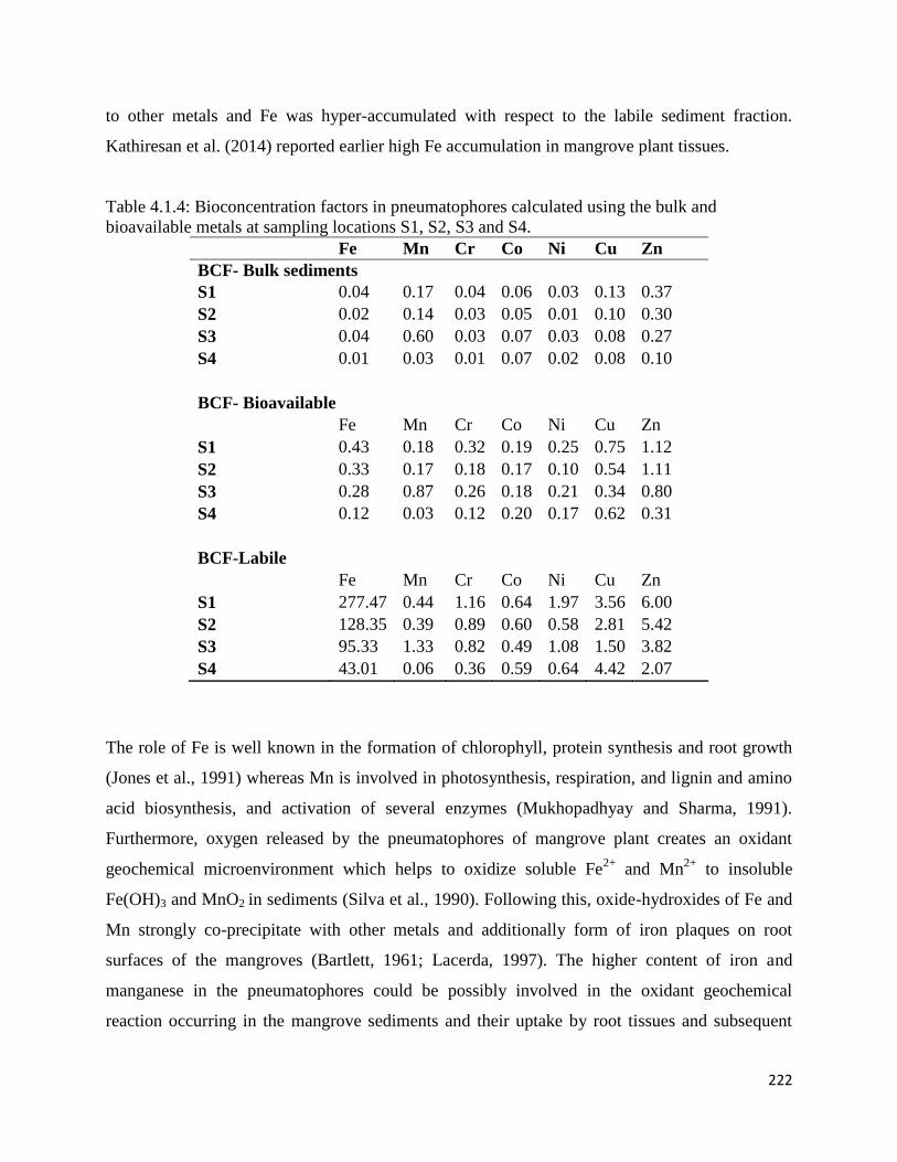
222
to other metals and Fe was hyper-accumulated with respect to the labile sediment fraction.
Kathiresan et al. (2014) reported earlier high Fe accumulation in mangrove plant tissues.
Table 4.1.4: Bioconcentration factors in pneumatophores calculated using the bulk and
bioavailable metals at sampling locations S1, S2, S3 and S4.
Fe Mn Cr Co Ni Cu Zn
BCF- Bulk sediments
S1 0.04 0.17 0.04 0.06 0.03 0.13 0.37
S2 0.02 0.14 0.03 0.05 0.01 0.10 0.30
S3 0.04 0.60 0.03 0.07 0.03 0.08 0.27
S4 0.01 0.03 0.01 0.07 0.02 0.08 0.10
BCF- Bioavailable
Fe Mn Cr Co Ni Cu Zn
S1 0.43 0.18 0.32 0.19 0.25 0.75 1.12
S2 0.33 0.17 0.18 0.17 0.10 0.54 1.11
S3 0.28 0.87 0.26 0.18 0.21 0.34 0.80
S4 0.12 0.03 0.12 0.20 0.17 0.62 0.31
BCF-Labile
Fe Mn Cr Co Ni Cu Zn
S1 277.47 0.44 1.16 0.64 1.97 3.56 6.00
S2 128.35 0.39 0.89 0.60 0.58 2.81 5.42
S3 95.33 1.33 0.82 0.49 1.08 1.50 3.82
S4 43.01 0.06 0.36 0.59 0.64 4.42 2.07
The role of Fe is well known in the formation of chlorophyll, protein synthesis and root growth
(Jones et al., 1991) whereas Mn is involved in photosynthesis, respiration, and lignin and amino
acid biosynthesis, and activation of several enzymes (Mukhopadhyay and Sharma, 1991).
Furthermore, oxygen released by the pneumatophores of mangrove plant creates an oxidant
geochemical microenvironment which helps to oxidize soluble Fe2+
and Mn2+
to insoluble
Fe(OH)3 and MnO2 in sediments (Silva et al., 1990). Following this, oxide-hydroxides of Fe and
Mn strongly co-precipitate with other metals and additionally form of iron plaques on root
surfaces of the mangroves (Bartlett, 1961; Lacerda, 1997). The higher content of iron and
manganese in the pneumatophores could be possibly involved in the oxidant geochemical
reaction occurring in the mangrove sediments and their uptake by root tissues and subsequent
223
accumulation in other plant tissues as suggested by Kathiresan et al. (2014). Copper is an
essential micronutrient required in the mitochondria and chloroplast reactions, enzyme systems
related to photosystem II electron transport, cell wall lignification, carbohydrate metabolism, and
protein synthesis (Verkleij and Schat, 1990). Zinc is also an essential micro-nutrient of numerous
enzyme systems, respiration enzyme activators, and the biosynthesis of plant growth hormones
(Ernst et al., 1992). Thus possibly essential elements viz. Fe, Mn, Zn and Cu were more bio-
accumulated compared to Co, Cr and Ni. Cr, Ni and Co are considered as non-essential elements
and toxic to plant growth (Bonanno and Giudice, 2010; He et al., 2014). Between the two
species, Avicennia officinalis accumulated higher metal concentrations in pneumatophore tissues.
Similar observation was made earlier by Sarangi et al. (2002) wherein metal concentrations in
five mangrove species were studied and A. officinalis accumulated highest concentrations of
metals analyzed. A. officinalis tends to manage the uptake of essential metals to fulfil metabolic
requirements while restricting the uptake of non-essential metals to avoid toxicity (Chakraborty
et al., 2013). The low accumulation of metals in S. alba pneumatophores than A. officinalis is
likely due to physiological differences and variations that exist in accumulation strategies of
different plant species (Defew et al., 2005). The variations in metal accumulation between the
two species and location in the estuary might be due to the metal need of the specific tissues,
variation in salinity, the amount/quantity of metals deposition in the mangrove sediments and
seawater intrusion during high tide as observed by Edu et al. (2015). In addition, the plant
species, types of plant components, physiological age of tissue and seasons likewise, have
significant influence on metal accumulation ability of the plants (Jones, 1998). Thus, the effects
of biological and physical phenomena, such as tidal inundation, salinity changes, wind and
waves that allow the processes of bioturbation, re-suspension and erosion and affect the metal
concentrations in sediments (Bellucci et al., 2002), may have a large influence on the uptake
and accumulation ability of metals by the mangrove plants.
The labile fraction of the sediments is anthropogenically influenced and is easily available to
biota. High uptake and accumulation of labile Fe, Cu and Zn by the mangrove plants suggest
their potential phytoremediation ability and thus act as long term sinks for metals.
Phytoextraction of contaminants from sediments requires translocation from root to other plant

224
parts and hyper-accumulation of contaminants requires species tolerant to high concentrations of
bioavailable metals (MacFarlane et al., 2007).
Pearson’s correlation of metal concentrations in pneumatophores versus average metal
concentrations of bulk sediments, bioavailable fraction and labile fraction was computed.
Statistically significant correlation (p<0.005, n=7) was obtained for the data set of bulk
sediments and bioavailable fraction. For core S1, r=0.98; p=0.0001 was obtained for metals in
pneumatophore with bulk sediments and r=0.94; p=0.0014 for metals in pneumatophores with
bioavailable fraction. For core S2 pneumatophores with bulk, r=0.99; p=0.00004 and
pneumatophores with bioavailable, r=0.98; p=0.0001 values were obtained. For core S3,
pneumatophore with bulk, r=0.97; p=0.0003 and pneumatophore with bioavailable, r=0.98;
p=0.00007 and for S4, pneumatophores with bulk, r=1.00; p=0.0000001 and pneumatophore
with bioavailable, r=0.97, p=0.0004 values were obtained. Hence, the strong correlation
indicated that pneumatophores are able to accumulate metals in accordance to the metal content
deposited in the underlying sediments. Pneumatophores are perennial organs that have a longer
duration of accumulation of trace elements as they contain high concentrations of tannins
compared to other tissue types, which provides a greater ability to bind trace metals (Silva et al.,
1990; Zheng et al., 1997; Ismail, 2002). Nath et al. (2014) found a strong positive relationship
between metals in sediments and pneumatophores that suggest the potential use of
pneumatophore tissues as a bio-indicator of estuarine contamination. Pearson’s correlation test
showed no significant correlation with respect to the labile fraction of sediments, i.e. r=0.09;
p=0.84 for core S1; r=0.04; p=0.93 for core S2; r=0.14; p=0.76 for core S3, and, r= -0.73; p=0.88
for S4. The poor correlation of metal concentrations in pneumatophores and metals in the labile
fraction may be due to the low concentration of metals in the labile fraction of sediments and
their subsequent uptake, translocation and storage in other plant parts such as root, bark and
leaves.
Thus, mangrove plants accumulated Fe, Mn, Cu and Zn in their pneumatophores tissues and
exhibited differences in accumulation of metal with respect to location and species due the
spatial variation in sediment characteristics, quantity of metals deposited in the sediments, their
bioavailability and differences in plant species and tissue physiology.

225
4.2 Bioaccumulation of metals in sediment associated biota
Sediments are sinks for heavy metals in estuarine/marine environments and play a key role in the
transmission and deposition of metals (Bastami et al., 2015). Sediments may contain higher than
average abundances of metals due to input from anthropogenic activities, which may cause the
formation of the more bioavailable forms of the metals. Benthic organisms can take up the
bioavailable fraction of metals from the sediments and accumulate them in their tissues that can
cause toxicity. Such effects can significantly affect the trophic structure of a biological
community. The metals deposited in the sediments at the water-sediment interface are important
to the fauna as compared with subsurface sediments since most fauna live above the reduced
zone in sediments. Therefore, the composition of surface sediments has a significant influence on
the living conditions of marine organisms. Thus, establishing a correlation between metal form
and concentrations in sediments and their uptake by biota is important to understand the impact
of sediment contaminants in the food chain in estuarine environments (Birch et al., 2014).
The molluscs are a diverse and species–rich phyla of the animal kingdom wherein gastropods
make up more than 80 % of the species and bivalves constituting a major part (15 %) of the rest
(Oehlmann and Schulte-Oehlmann, 2003). They are common, macroscopic, ecologically and
commercially important on a global scale as food and as non-food resources (Palpandi and
Kesavan, 2012). Molluscs are in direct contact with the ambient medium (water or sediment) due
to the lack of an exoskeleton and can assimilate contaminants not only from the diet via the
gastro-intestinal tract but also from ambient water or sediment via the integument and respiratory
organs resulting in greater contaminant accumulation potential. They are being successfully
applied as biological indicators due to their effective accumulation of organic and metallic
pollutants in their tissues at concentrations several orders of magnitude above those observed in
the field environment (Elder and Collins, 1991; Bryan et al., 1983). Bivalves and gastropod
molluscs are also considered as useful biomonitors of certain metals. Most metals are generally
concentrated many times higher within an organism’s soft tissue, rather than the shell (Kesavan
et al., 2013). The objective of the present study was to estimate the heavy metal concentrations
such as Fe, Mn, Cr, Co, Ni, Cu, and Zn, in the soft tissues of molluscs collected from different
locations along the Zuari estuary and explore the potential of using these molluscs as a

226
bioindicator for metal accumulation. The different species collected from the sedimentary
environments are listed in table 4.2.1.
Table 4.2.1: Sediment associated biota collected from the intertidal environments of the Zuari
estuary.
Sample
location
Subenvironment Species Phyllum Class
S2 Mangrove Neritina (Dostia)
violacea
Mollusca Gastropoda
M3 Mudflat Telescopium telescopium Mollusca Gastropoda
Crassostrea sp. Mollusca Bivalvia
Muricidae sp. Mollusca Gastropoda
Neritina (Dostia)
violacea
Mollusca Gastropoda
M4 Mudflat Cerithidea quadrata Mollusca Gastropoda
Telescopium telescopium Mollusca Gastropoda
Crassostrea sp. Mollusca Bivalvia
In Zuari estuary, one gastropod species Neritina (Dostia) violacea was collected from the
Cumbharjua canal mangrove S2, two gastropods Telescopium telescopium and Muricidae sp.
and one bivalve belonging to genus Crassostrea was collected from M3 mudflat and three
gastropods Neritina (Dostia) violacea, Cerithidea quadrata and Telescopium telescopium and
bivalves belonging to genus Crassostrea were collected at M4 mudflat (Table 4.2.1).
The concentration of metals Fe, Mn, Cr, Co, Ni, Cu, and Zn determined in bulk sediments,
bioavailable and labile fractions in the year 2015 post-mining ban collection (Table 4.2.2) was
used for comparison and calculation of various indices. Highest bulk metal concentration of Fe,
Co and Ni were noted in S2, Cr and Cu in M3 and Mn and Zn in M4. Metals in the bioavailable
fractions showed greater abundance for Co and Ni at S2, Fe and Cu at M3 and Mn, Cr and Zn at
M4. The labile fraction of metals showed higher content of Co and Cu at M3 and Fe, Mn, Cr, Ni
and Zn at M4. Overall, abundance of metals in the sediments decreased in the order of Bulk
sediments> bioavailable> labile.

227
Table 4.2.2: Concentration of metals Fe, Mn, Cr, Co, Ni, Cu and Zn determined in bulk
sediments, bioavailable and labile fractions in the 2015 post-mining ban collection and Apparent
effects threshold (AET) in sediments for Benthic invertebrate and Oysters (Gries and Waldow,
1996).
Fe Mn Cr Co Ni Cu Zn
Ppm Ppm Ppm Ppm Ppm ppm ppm
Bulk
sediments
S2 107945 3800 273 57.00 154 119 128
M3 99015 2910 281 51.40 138 130 138
M4 102595 4235 268 45.25 122 120 146
Bioavailable
S2 7852 3165 40.13 18.61 21.95 21.32 34.17
M3 9466 2754 33.87 16.75 17.87 23.20 41.43
M4 7475 3656 40.23 15.17 17.46 20.37 46.36
Labile
S2 20.34 1355 7.94 5.20 3.62 4.10 7.00
M3 22.85 1308 12.60 5.47 2.70 6.30 6.71
M4 67.76 1673 15.03 5.34 4.72 4.85 8.07
Benthic AET NA NA 260 NA >140 530 410
Oyster AET NA NA NA NA NA 390 1600
The concentrations of metals in bulk, bioavailable, and labile fractions were compared with the
Apparent effects threshold (AET) of benthic invertebrates and oysters. The AETs are
concentrations of specific metals of concern in sediments above which a significant adverse
biological effect always occurs. The concentration of Cr in bulk sediments was above the AET
for benthic invertebrates at S2, M3, and M4; and concentration of Ni at S2 was above the AET
for benthic in vertebrates when compared to the standard values available (Gries and Waldor,
1996).
The concentration of metals in the benthic organisms was observed to vary spatially and among
the different species (Table 4.2.3). Overall, the organisms showed significantly higher
concentrations of Fe, Mn, Cu and Zn in their tissues whereas Cr, Co and Ni were accumulated in
lesser amounts.

228
Table 4.2.3: The concentration of metals in tissues of the sediment associated biota in mangrove
S2 and mudflats M3 and M4.
Fe Mn Cr Co Ni Cu Zn
ppm Ppm ppm Ppm ppm ppm ppm
S2 Neritina (Dostia)
violacea 2276 517 11.43 17.68 22.67 23.67 190
M3 Telescopium
telescopium 2640 782 7.12 6.67 8.67 213 237
Crassostrea sp. 939 170 4.15 4.79 5.39 341 804
Muricidae sp. 1183 166 13.01 7.33 ND 1994 556
M4 Neritina (Dostia)
violacea 2095 440 8.17 13.53 12.98 23.35 161
Crassostrea sp. 1348 74.91 4.49 3.65 1.30 207 1525
Cerithidea quadrata 978 414 5.94 10.68 12.78 74.57 69.75
Telescopium
telescopium 517 1229 3.53 6.17 9.00 161 409
ND- Not detectable
Highest concentrations of Fe (2640 ppm) were found in tissues of T. telescopium at M3, Mn
(1229 ppm) in T. Telescopium of M4, Cr (13.01 ppm) and Cu (1994 ppm) in Muricidae sp. of
M3, Co (17.68 ppm) and Ni (22.67 ppm) in N. violacea of S2 and Zn (1525 ppm) in Crassostrea
sp. of M4. The concentration of metals varied in the order Fe>Mn>Zn>Cu>Ni>Co>Cr in N.
violacea at S2. At M3, metals varied in the order of Fe>Mn>Zn>Cu>Ni>Cr>Co in T.
Telescopium, Fe>Zn>Cu>Mn>Ni>Co>Cr in Crassostrea sp. and Fe>Cu>Zn>Mn>Cr>Co>Ni in
Muricidae sp. At M4, metals concentrations varied in the order of Fe>Mn>Zn>Cu>Co>Ni>Cr in
N. violacea, Zn>Fe>Cu>Mn>Cr>Co>Ni in Crassostrea sp., Fe>Mn>Cu>Zn>Ni>Co>Cr in C.
quadrata, Mn>Fe>Zn>Cu>Ni>Co>Cr in T. telescopium. N. violacea of the Cumbharjua canal S2
accumulated higher content of metals Fe, Mn, Cr, Ni, Co, Cu and Zn than the same species
collected from the mudflat of the lower middle estuary. T. telescopium of M3 accumulated higher

229
content of Fe, Cr, Co and Cu whereas T. telescopium of M4 had higher content of Mn, Ni and Zn
in its tissues. Crassostrea sp. of M3 had higher concentration of Mn, Co, Ni, and Cu in their
tissues whereas Fe, Cr and Zn were higher in Crassostrea sp. of M4.
The concentration of metals in the biota was compared with the concentration of metals in the
bulk sediments, bioavailable, and labile fractions. The concentration of Fe ranged from 99015
ppm to 107945 ppm in the bulk sediments, 7475 ppm to 9466 ppm in the bioavailable fraction
and 20.34 ppm to 67.76 ppm in the labile fraction of the sediments whereas Fe in the tissues of
the molluscs ranged from 517 ppm to 2640 ppm, highest being in T. telescopium at M3. Mn
concentrations in the sediments ranged from 2910 ppm to 4235 ppm in the bulk sediments, 2754
ppm to 3656 ppm in the bioavailable fraction and 1308 ppm to 1673 ppm in the labile fraction
while Mn in the mollusc’s tissues varied from 74.91 ppm to 1229 ppm, highest being in T.
telescopium at M4. The concentration of Cr varied from 268 ppm to 281 ppm in the bulk
sediments, 33.87 ppm to 40.23 ppm in the bioavailable fraction and 7.94 ppm to 15.03 ppm in
the labile fraction whereas Cr in the molluscs tissues ranged from 3.53 ppm to 13.01 ppm,
highest being in Muricidae sp. at M3. Co concentration in the sediments ranged from 45.25 ppm
to 57.00 ppm in the bulk sediments, 15.17 ppm to 18.61 ppm in the bioavailable fraction and
5.20 ppm to 5.47 ppm in the labile fraction while Co in molluscs tissues varied from 3.65 ppm to
17.68 ppm, highest being in N. violacea at S2. Ni concentration in the sediments varied from 122
ppm to 154 ppm in the bulk sediments, 17.46 ppm to 21.95 ppm in the bioavailable fraction of
sediments and 2.70 ppm to 4.72 ppm in the labile fraction whereas Ni in the mollusc’s tissues
varied from 1.30 ppm to 22.67 ppm, highest being in N. violacea at S2. Cu in the sediments
ranged from 119 ppm to 130 ppm in the bulk sediments, 20.37 ppm to 23.20 ppm in the
bioavailable fraction and 4.10 ppm to 6.30 ppm in the labile fraction whereas Cu in the tissues
ranged from 23.35 ppm to 1994 ppm, highest being in Muricidae sp. at M3. Zn concentration in
the sediments ranged from 128 ppm to 146 ppm in bulk sediments, 34.17 ppm to 46.36 ppm in
bioavailable fraction and 6.71 ppm to 8.07 ppm in the labile fraction whereas Zn in molluscs
tissues varied from 69.75 ppm to 1525 ppm, highest being in Crassostrea sp. at M4.
Overall, Fe and Mn concentrations were highest in the mollusc’s tissues, which may have been
due to its high bioavailability in the sediments resulting in increased uptake by biota. Cu and Zn

230
concentrations were higher in the mollusc’s tissues than the sediments, which indicated that Cu
and Zn were, taken up in large amounts and were bioaccumulated in the organism tissues. Cr,
Co, and Ni were taken up in low concentrations by the organisms due to their low bioavailability
in the sediments.
The Biota Sediment Accumulation Factor (BSAF) of metals was calculated which described the
bioaccumulation of the sediment-associated metals into tissues of ecological receptors. The
BSAF values (Table 4.2.4) with respect to the bulk sediments showed that T.telescopium,
Crassostrea sp. and Muricidae sp. at M3, and Crassostrea sp. and T. telescopium at M4 showed
values greater than 1.00 for Cu. Further, all the sampled organisms at the three locations, except
for C. quadrata at M4, exhibited values greater than 1.00 for Zn. The BSAF values for Fe, Mn,
Cr, Co and Ni were less than 1.00 for all collected biota samples. Higher BSAF values were
noted with respect to the bioavailable metal concentrations as compared to the bulk metal
concentrations. Cu and Zn showed high BSAF values ranging from 1.00 to 85.96 in the species
collected at the three locations. Fe, Mn, Cr, Co and Ni exhibited BSAF values less than 1.00,
except for Ni for N. violacae (1.03) at S2. BSAF values were also calculated using the labile
fraction of the sediments. The BSAF values varied from less than 1.00 to as high as 317. The
BSAF values of Fe, Zn and Cu were greater than 1.00 for all species at the three locations in
addition to Cr, Co and Ni for some species. N. violacea at S2 showed BSAF values greater than
1.00 for Fe, Cr, Ni, Cu, and Zn. At M3, T. telescopium exhibited BSAF values greater than 1.00
for Fe, Co, Ni, Cu and Zn, Crassostrea sp. for Fe, Ni, Cu and Zn, and Muricidae sp. for Fe, Cr,
Co, Cu and Zn. At station M4, N. violacea exhibited BSAF values greater than 1.00 for Fe, Co,
Ni, Cu and Zn, Crassostrea sp. for Fe, Cu and Zn, C. quadrata and T. telescopium for Fe, Co,
Ni, Cu and Zn. From the computed BSAF values, it is clear that Crassostrea sp. and Muricidae
sp. accumulated large amount of Cu and Zn.

231
Table 4.2.4: Biota Sediment Accumulation Factor (BSAF) calculated relative to concentrations
of bulk metals, bioavailable metals and labile metals.
Station
n
Organism Fe Mn Cr Co Ni Cu Zn
BSAF-Bulk
metals
S2 N.violacea 0.02 0.14 0.04 0.3
1
0.15 0.20 1.49
M3 T. telescopium 0.03 0.27 0.03 0.1
3
0.06 1.63 1.72
Crassostrea sp. 0.01 0.07 0.01 0.0
9
0.04 2.62 5.82
Muricidae sp. 0.01 0.06 0.05 0.1
4
--
0.01 15.33 4.03
M4 N. violacea 0.02 0.10 0.03 0.3
0
0.11 0.20 1.10
Crassostrea sp. 0.01 0.02 0.02 0.0
8
0.01 1.73 10.47
C. quadrata 0.01 0.10 0.02 0.2
4
0.10 0.62 0.48
T. telescopium 0.01 0.29 0.01 0.1
4
0.07 1.34 2.81
BSAF-
Bioavailable
S2 N.violacea 0.29 0.16 0.28 0.9
5 1.03 1.11 5.57
M3 T. telescopium 0.28 0.28 0.21 0.4
0
0.49 9.16 5.73
Crassostrea sp. 0.10 0.07 0.12 0.2
9
0.30 14.72 19.40
Muricidae sp. 0.12 0.06 0.38 0.4
4
--
0.09 85.96 13.42
M4 N.violacea 0.28 0.12 0.20 0.8
9
0.74 1.15 3.46
Crassostrea sp. 0.18 0.02 0.11 0.2
4
0.07 10.15 32.89
C. quadrata 0.13 0.11 0.15 0.7
0
0.73 3.66 1.50
T. telescopium 0.07 0.34 0.09 0.4
1
0.52 7.89 8.82
BSAF-
Labile
S2 N.violacea 112 0.38 1.44 3.4
0
6.26 5.78 27.20
M3 T. telescopium 116 0.60 0.57 1.2
2
3.21 33.74 35.37
Crassostrea sp. 41.09 0.15 0.33 0.8
8 2.00 54.20 120
Muricidae sp. 51.75 0.13 1.03 1.3
4
--
0.61 317 82.89
M4 N. violacea 30.91 0.26 0.54 2.5
3
2.75 4.81 19.89
Crassostrea sp. 19.90 0.04 0.30 0.6
8
0.28 42.64 189
C.quadrata 14.44 0.25 0.40 2.0
0
2.71 15.37 8.64
T. telescopium 7.63 0.73 0.23 1.1
6
1.91 33.14 50.68
The metal pollution index (MPI) was calculated using the equation MPI= (Cf1 x Cf2 x Cf3….x
Cfn) 1/n
where Cfi is the concentration of metal in the sample and the results were presented in
table 4.2.5. The MPI revealed that gastropods tend to accumulate more metals in their tissues
than bivalves-Crassostrea sp.

232
Table 4.2.5 :Metal pollution index (MPI) for organism collected from the intertidal environments
along the Zuari estuary.
Sample
location
Organism MPI N
S2 N. violacea 81.69 7
M3 T. telescopium 88.62 7
Crassostrea sp. 65.63 7
Muricidae sp. 166 6
M4 N. violacea 65.10 7
Crassostrea sp. 48.99 7
C. quadrata 55.91 7
T. telescopium 69.95 7
The analysis of the metals content in the tissues, along with BSAF and MPI of the mollucs
revealed that the sediment-associated biota accumulated more Fe, Mn, Cu, and Zn over Cr, Co
and Ni. Fe, Mn, Cu, and Zn are considered as essential elements whereas Cr, Co and Ni are non-
essential but are required for metabolism in trace quantities and both essential and non-essential
metals are taken up from water, sediment, or food, by the benthic organisms. Essential elements
Fe, Mn, Cu, and Zn are important for the metabolism of the organism. Iron is associated with
various enzymes in living systems such as peroxidase, catalase, cytochrome, oxidase,
nitrogenase (Cole, 1983). Cu and Zn play an important role in the composition of approximately
90 enzymes in animal metabolism (Carvalho et al., 1993). Mn though available in high
concentrations in the sediment bioavailable fractions and tissues, showed low BSAF values,
which may indicate the slowing of Mn uptake after reaching the maximal level of this metal in
the organisms
The enhanced accumulation of Fe, Mn, Zn, and Cu in organisms may be due to sequestration of
metal cations in insoluble metal- rich granules and cellular metal detoxification/redistribution
(Viarengo and Nott, 1993; Irato et al., 2003). The rates of metal uptake and excretion are affected
by the biology of the organism, the permeability of the external surface, the nature of food, and
the efficiency of the osmoregulational system present (Rainbow, 1995). The scrap metals from
the boat metals and fishing vessels and paint residues (antifouling paints) from local boat jetties
may be the source of zinc and copper to the sediment and which is taken up by the organism and

233
accumulated in the tissues (Palpandi and Kesavan, 2012). Fe in the labile fraction is directly
related to anthropogenic metal inputs exhibited higher BSAF, which may be from leachates of
mining ores. BSAF values for Mn were low which may be due to homoestasis (internal
regulation) of metals by the organisms (Fasulo et al., 2008).
The differences between BSAF and MPI in the different molluscs species may be related to the
differences in the detoxification mechanisms and/or metabolic activities (Azevedo et al., 2012).
It is known that accumulation of metals in large concentrations can cause toxicity to the
organism. However, the organisms have regulatory and detoxification mechanisms. Some
metalloproteins are known by their function in detoxification such as Metallothioneins which are
low-molecular-weight cytosolic proteins with a high cysteine content, showing a strong affinity
towards certain essential and nonessential trace elements, such as Cu and Zn (Kägi and Schäffer,
1988) and, therefore, make them less toxic to other cellular constituents (HEATH, 1990). Zn and
Cu are known as essential elements that activate many enzymatic systems. Zn especially has an
important function since it is a component of metallothionein. This protein is very important in
the detoxification of toxic metals through the dismutation of zinc-binding (Smirnov et al., 2005).
Since molluscs have a limited ability to excrete pollutants, metabolize organic chemicals, and
physiologically inactivate toxic metals by binding to metallothioneins, the molluscs tend to attain
higher bioaccumulation factors for many metals (Berger et al., 1995, Oehlmann and Schulte-
Oehlmann, 2003).
Thus, benthic invertebrates are important in the assessment of ecological risks of aquatic sites.
One of the primary contaminant exposure pathways for these organisms is the consumption of
contaminated food. Deposited sediments often act as a local sink for contaminants, which may
increase the contaminant exposure for sediment associated biota that ingest sediment particles
while foraging. These sediment benthic invertebrates are an important food source for fish and
some terrestrial wildlife. Therefore, the concentrations of bioavailable contaminants in sediment
revealed the food chain transfer and the potential toxicity of sediment contaminants (Jacobs,
1998). The metals in sediments are not always bioavailable, since their bioavailability depends
on a series of factors such as pH, Eh, granulometry and organic matter content. Nonetheless,

234
metals in the environment are taken up by the organisms and can accumulate in tissues (HEATH,
1990).
Table 4.2.6: Pearson’s correlation coefficient (r) and significance (p) of metals in tissues with
bulk sediments, bioavailable and labile fraction of metals.
Species Sampling
location
Metal correlation r p
N. violacae S2 Tissue/ bulk sediment 0.98 <0.05
Tissue/bioavailable metals 0.98 <0.05
Tissue/labile metals 0.05 >0.05
M4 Tissue/ bulk sediment 0.99 <0.05
Tissue/bioavailable metals 0.96 <0.05
Tissue/labile metals 0.06 >0.05
T. telescopium M3 Tissue/ bulk sediment 0.97 <0.05
Tissue/bioavailable metals 0.99 <0.05
Tissue/labile metals 0.12 >0.05
M4 Tissue/ bulk sediment 0.22 >0.05
Tissue/bioavailable metals 0.59 >0.05
Tissue/labile metals 0.90 <0.05
Crassostrea sp. M3 Tissue/ bulk sediment 0.68 >0.05
Tissue/bioavailable metals 0.65 >0.05
Tissue/labile metals -0.15 >0.05
M4 Tissue/ bulk sediment 0.58 >0.05
Tissue/bioavailable metals 0.45 >0.05
Tissue/labile metals -0.23 >0.05
Muricidae sp. M3 Tissue/ bulk sediment 0.32 >0.05
Tissue/bioavailable metals 0.24 >0.05
Tissue/labile metals -0.30 >0.05
C. quadrata M4 Tissue/ bulk sediment 0.93 <0.05
Tissue/bioavailable metals 0.99 <0.05
Tissue/labile metals 0.27 >0.05
When Pearson’s correlation of metals in tissue with metals in the bulk, bioavailable and labile
fractions was computed (Table 4.2.6), N. violacae showed significant correlation of metals in

235
tissue with the bulk sediments and bioavailable fractions at locations S2 and M4. T. telescopium
exhibited significant positive correlations of metals in tissue with metals in bulk sediments and
bioavailable fraction at M3 and metals in sediments with labile fraction in M4. C. quadrata
showed significant correlation of metals with the bulk sediment and bioavailable fractions.
Crassostrea sp. and Muricidae sp. did not show any significant relation of metals in tissues with
metals in sediments.
N. violacae exhibited consistency in its correlation of metals in tissue with bulk and bioavailable
metals at both sample locations along with high MPI at S2 and M4, which may suggest its use as
a bioindicator since it tends to accumulate metals relative to that available in the sediments. T.
telescopium and C. quadrata also exhibited significant correlation of metals in tissue with bulk
and bioavailable metals and showed high MPI suggesting their ability in biomonitoring of
metals. The bivalve Crassostrea did not show any significant correlation of metals in tissues
with sediments, along with lowest MPI at M3 and M4, Muricidae sp. exhibited poor correlation
of metals in tissues with metals in sediments but with high MPI. Thus, gastropods N. violacae, T.
telescopium, and C. quadrata can be used as potential bioindicators in the estuarine environment
since they reflect the conditions of the local environment.
The bioaccumulation study showed that there were evidences of bioaccumulation of metals Fe,
Cu and Zn in the biota of the Zuari estuary. However, information on the impact of pollutants on
biota can only be obtained by applying long-term in situ biomonitoring assays (Bervoets et al.,
2004) due to fluctuations in anthropogenic metal inputs and estuarine dynamics,
physicochemical processes and changes in macrofauna community structure. Thus, long-term
studies should be carried out to continuously monitor the estuarine quality and identify potential
threats to the estuarine fauna.

236
Chapter 5
Summary
and
Conclusions
237
Mudflats and mangroves are important estuarine sub-environments, found in the inter-tidal zone
of tropical and subtropical coasts. The mangrove and mudflats receive large contaminant inputs
from catchments derived from run-off, anthropogenic leachates and discharges, as well as
atmospheric and marine inputs. Consequently these environments have become important sinks
for nutrients, organic and inorganic contaminants. Among these pollutants, metals have received
significant attention due to their long-term effects on the environment. Metals originating from
both natural and anthropogenic sources are discharged into estuarine system, which are
transported and distributed in the aqueous phase and sediments. Physicochemical processes like
adsorption and co-precipitation cause deposition of large quantity of metals to the sediment.
Additionally, sediment parameters like sediment size, mineralogy, salinity, pH, organic matter
content and oxidation–reduction potential are important parameters controlling the accumulation
and the availability of metals in the sediment.
The Zuari estuary, located on the west coast of India is one of the major estuaries in Goa. Its
catchment area is known for open cast iron and ferromanganese mines and is used to transport
iron ores to the Mormugao harbor located at the mouth of the Zuari estuary. Mining in Goa has
resulted in an environmental threat that was first felt in the year 1978 and as a consequence 287
mining concessions/leases were terminated and again in the year 2012, that led to a complete ban
on mining. Several jetties, barge building and repairing industries, constructions and domestic
waste discharges along the estuary release a large amount of organic and inorganic contaminants
to the estuary. The Cumbharjua canal links the Zuari estuary to the adjacent Mandovi estuary and
adds more mining material to the Zuari during the monsoons and ebb tide. These contaminants
accumulate in the estuarine sediments over long periods and degrade the environmental quality
and cause detrimental effect to the estuarine ecosystems. The estuarine sediments thus record the
regional environmental changes and anthropogenic impacts. A geochemical investigation of
estuarine sediment should illustrate the distribution, source, and enrichment of chemical elements
in relation to sedimentary processes in the estuary. With this background the following objectives
of the study were formulated:

238
1. To study the abundance and distribution of metals in sediments and to understand the
role of physicochemical and geochemical parameters influencing the distribution of
metals.
2. To study the concentration of metals in soft tissue of selected biota associated with sediments.
3. To establish a relation between bioavailability of metals in sediments and bioaccumulation of
metals in biota.
To fulfil the above objectives, sediment grain size, total organic carbon, clay mineralogy,
magnetic susceptibility parameters and bulk and clay metal chemistry and fractionation of metals
was carried out on sediment cores, seasonal surface samples along with metal accumulation in
biota. Four sampling locations in the Zuari estuary were selected from which one mudflat and
mangrove from the upper middle estuary, lower middle estuary and lower estuary and one
mangrove from the Cumbharjua canal were sampled. Furthermore, to understand the depositional
environment, metal association and possible sources, statistical analysis of Pearson’s correlation,
principal component analysis and isocon diagrams were used. Pollution indices of enrichment
factor, geoaccumulation index were used to know the metal contamination status of the estuary.
Furthermore, geochemical speciation of metals into five fractions was carried out to understand
the mobility and bioavailability of metals in the sediments. The contamination of metals in
different sediment fractions was compared with sediment quality guidelines to determine the
toxity risk to biota.
The sediment cores of approximately 40 cm were collected from mudflat and mangrove
environments of the upper middle estuary, lower middle estuary and lower estuary and one
mangrove from the Cumbharjua canal in 2011 during premonsoon season. In the mangrove
environments, finer sediments, organic matter and metals were higher in the middle estuary and
canal sediments while coarser sediments with fewer metal concentrations were seen in the lower
estuary. The hydrodynamic conditions changed from lower estuary towards the upstream regions
owing to mixing of riverine and sea water that led to finer sediment deposition in the middle
estuary. Kaolinite, smectite, illite and traces of chlorite constituted the clay mineral assemblage

239
and had a minor influence on metal distributions. Magnetic susceptibility measurements
indicated that there are substantial inputs of mining material into estuary mainly in the upper
middle estuary and Cumbharjua canal. The variations in metal abundance were attributed to a
difference in hydrodynamic conditions regulated by the tide, freshwater flow and
geomorphology of the Zuari estuary. The results revealed that the estuary received material from
natural weathering of rocks as well as from anthropogenic sources such as mining and
industrial/domestic discharges.
In the upper middle estuary, trace metal distribution was influenced by adsorption onto Fe-oxides
and flocculation in low salinity. In the Cumbharjua canal, there was substantial anthropogenic
input of metals that was transported from the Mandovi estuary during periods of high rainfall and
was accumulated in the sediments. The lower middle estuary mangrove showed little variations
in metal distribution patterns and sediment grain size as metals associated with suspended matter
may have been fully mixed and then deposited in this region. Hydrous Fe-oxides and
aluminosilicates influenced the distribution patterns of metals in the sediments. Metals were less
concentrated at the lower estuary mangrove, which was due to intensive tidal washing and
dilution of metals by coarser sediments. However, the metals were associated with the finer
sediments. Al, Fe and Mn distributions indicated lithogenic source. Correlation analysis of bulk
metals with the clay minerals revealed that Cr was associated with chlorite in core S1 whereas Ni
was associated with kaolinite and Zn was associated with smectite in core S2. Metals did not
show significant association with the clay minerals in cores S3 and S4. Salinity played a
significant role in the association of Ni with kaolinite whereas Zn may have replaced Al in the
smectitic clays. Correlation analysis of magnetic susceptibility parameters and metals in the
mangrove sediments indicated that the iron ore mined and transported from the catchment areas
contributed ferrimagnetic particles to the sediments resulting in enhancement of magnetic
susceptibility. Comparison of metals in the clay fraction with bulk metals in the mangrove
sediments showed that most trace metals were enriched in the clay fraction. Fe and to some
extent Co showed higher concentrations in the bulk suggesting their association with the larger
sized sediments of sand and silt. Enrichment factor and Geo-accumulation index showed that Fe,
Mn and Cr were enriched in the mangrove sediments. Fractionation of metals Fe, Mn, Cr, Co, Cu
and Zn revealed that concentrations of bioavailable Mn pose a considerable risk to biota. Metals

240
Fe, Cr, Co, Cu and Zn were associated with the residual fraction of the sediments and thus have a
major detrital control.
The mudflat cores collected from the upper middle estuary, lower middle estuary and lower
estuary were also analyzed for sediment components, clay mineralogy, magnetic susceptibility
and metal geochemistry and fractionation. The mudflat sediments along the estuary were
dominated by silt and clay. The lower estuary sediments had higher percentage of coarse
sediments whereas higher clay was noted in the lower middle estuary. This distribution of grain
size was influenced by hydrodynamic conditions which are stronger towards the mouth and
becomes calmer towards the upstream regions. Organic matter was higher in the upper middle
estuary either due to the high content of finer sized sediments, inputs from sewage and
wastewater or lower hydrodynamics. Clay mineralogy analysis of the mudflat sediments revealed
that kaolinite was the most abundant clay mineral and was enriched in the upper middle estuary,
whereas Smectite was high in the lower estuary and illite and chlorite was abundant in the lower
middle estuary and their distribution varied due to estuarine dynamics, flocculation and stability
properties of the clay minerals. Analysis of magnetic susceptibility parameters of the mudflat
sediments indicated that the upper middle estuary contained higher amount of magnetic material
than other regions of the estuary. Among metals, most were accumulated in the upper middle
estuary than the mouth due to estuarine hydrodynamics, which increases towards the mouth
under the influence of strong waves. In the upper middle estuary, metal distributions were
influenced by Fe-Mn oxides and organic matter and less influenced by sediment grain size.
Correlation analysis indicated that the metals were supplied from an anthropogenic source, as
they do not show significant correlation with Al. In the lower middle estuary, the influence of
sediment grain size and organic matter on metal distributions was noted to be negligible.
However it was noted that the mudflat sediments were undergoing early diagenetic processes.
The mudflat sediments of the lower estuary revealed that metal distributions were less affected by
sediment components and the most metals were of detrital origin and associated with
aluminosilicates. Poor correlation of bulk metals and clay minerals indicated the clay mineralogy
had very little influence on metal distribution and was more influenced by other sediment
components and physiochemical processes. The strong correlation between magnetic
susceptibility and several heavy metal concentrations suggests a significant contribution to the

241
magnetism from anthropogenic sources and revealed the metals may have been preferentially
adsorbed onto the exterior surface of Fe- oxides and precipitated to the sediments. The
comparison of metal concentrations in the bulk sediments and clay fraction, however, revealed
that most trace metals were enriched in the clay fraction of sediments and were associated with
aluminosilicates except for Fe, which was higher in the bulk sediments suggesting its association
with coarse sediments. Enrichment factor and Geoaccumulation indices revealed that the
mudflats sediments were contaminated by Fe, Mn and Cr. Speciation of metals Fe. Mn, Cr, Co,
Cu and Zn revealed that Fe, Cr, Co, Cu and Zn were associated with the residual phase and thus
have low mobility and bioavailability. However, bioavailable concentrations of Mn in the
sediments were considerably high indicating high potency for mobility and toxicity.
A comparison of mudflat and mangrove sediment components and metals was made using the
isocon diagram which revealed that, the variability in the distribution of metals and sediment
components within mudflats and mangroves increased towards the lower estuary and may be
attributed to the geomorphic characteristics and the physical processes in the estuary. In the upper
middle estuary, much of the sedimentary material is supplied and the narrow canal width and the
low tidal current magnitude facilitated quick removal of material from the water column to the
sediments. Fe-Mn oxyhydroxides and organic matter adsorbed trace metals in the mudflats
whereas in the mangroves, organic matter played a significant role in metal accumulation. In the
lower middle estuary, the relatively broader channel width that allows for an increased tidal
magnitude and thus may cause resuspension and re-deposition of sediments. Metals in the
mudflats were influenced by sand, clay Mn-oxides and whereas silt influenced metal distribution
in mangroves. In the lower estuary, the broad width of the bay and the high energy conditions
caused turbulence due to which much of the sediments are re-suspended and transported to
calmer regions. Hydrodynamics played as significant role in the lower estuary and most metals
were enriched in the mudflats sediments than mangroves due to higher fine sediments and Fe Mn
oxides. In general, the sediments of the mudflats were influenced by physico-chemical processes
whereas metals in the mangroves sediment were influenced by organic matter.
Differences in speciation of mudflat and mangrove sediments showed that the accumulation and
bioavailability of metals within sediments depends organic matter supply, salinity and sediment

242
particle size. Due to the high density of roots and a short period of flooding in the mangrove
forest environment, the redox conditions of vegetated sediments may be the main limiting factor
for bioavailability in mangroves. In tidal mudflats, where sediments are not aerated by oxygen
released from plant roots and higher moisture contents exist for longer periods of tidal
inundation, organic matter content becomes the important limiting factor for bioavailability
Surface sediments were collected in the premonsoon, monsoon and postmonsoon season. Metals
showed differential associations with different seasons in the Zuari estuary mangrove sediments.
During the pre-monsoon (dry) season, with high salinity intrusion, hydrous Fe-Mn oxides played
a role in the distribution of metals in the mangrove sediments. During the monsoon season, the
stratification of the estuary and large land runoff bring about large changes in physicochemical
properties of the estuarine waters and a large amount of material is transported into the estuary.
In the postmonsoon, there is a reduction in fresh water influx, accumulation of trace metals, is
related to fine sediments, organic matter and Mn oxides that were brought during the monsoons.
The metal distribution showed observable seasonal differences in the mudflat sediments of the
Zuari estuary. In the premonsoon season, enrichment of most trace metals in the upper middle
estuary sediments was due to the removal of metals during early estuarine mixing and proximity
of the sampling location to the metal sources. The sediment grain size, organic matter and
hydrous Fe-Mn oxides affected metal distributions. In the monsoon, trace metals were enriched
in the upper middle estuarine sediments along with fine sediments, organic matter and Mn oxides
due to the large influx of fresh sedimentary material from land runoff from the catchment area.
In the post-monsoon season, trace metals were enriched in the lower middle estuary along with
organic matter suggesting that these metals may be associated with increasing sewage effluxion.
Most metals showed least concentrations in the lower estuary. Resuspension of sediments may
have been a major process influencing metal distribution in the postmonsoon.
Sediments collected from the estuarine mangroves and mudflat environments of the Zuari
estuary and adjoining Cumbharjua canal in 2015 premonsoon season were analyzed to assess
concentration and bioavailability of metals in the estuarine environment after ban on mining.
Following the ban on mining, Fe concentrations in sediments decreased in the estuary with silt
243
whereas trace metals Mn, Cr, Co, Ni, Cu and Zn increased with the clay fraction of sediments.
Speciation studies revealed that Fe, Cr, Co, Ni, Cu and Zn were mainly of lithogenic origin, less
mobile and bioavailable and posed low risk to biota associated with the sediments. The high
content of Mn in the bioavailable fraction raised concerns over its potential mobility,
bioavailability and subsequent toxicity.
In the mudflat sediments, the spatial variations of metals in the sediments were attributed to
various hydrodynamic and physicochemical processes. A comparison of average values of
sediment components and metal concentration of 2011 and 2015 datasets revealed that the
concentrations of trace metals along with clay in the estuarine sediments had considerably
increased whereas Fe concentration along with silt and organic matter had decreased. The
increase in trace metals in the estuary may be related to anthropogenic inputs and their
redistribution in the sediments was facilitated by adsorption onto clay particles or formed coating
on sand particles. Additionally, resuspension of bottom sediments may have considerably
influenced the metal distribution. Speciation of metals revealed that Fe, Cr, Co, Ni, Cu and Zn
were concentrated in the residual phase indicating these metals are potentially less mobile and
pose a lower toxicity risk. Concentrations of bioavailable Mn in the estuary posed a high risk to
biota. A comparison of bioavailability of metals in post-mining ban period with pre-mining ban
revealed elevated concentration of metals in the bioavailable fractions in the post-mining ban
period and indicated increased anthropogenic inputs into estuary from the catchment area.
Although the mining in the catchment area has been stopped, the leachates of ore stored on the
river banks continue to enter into the estuary. In addition, input of metals from various sources,
couples with resuspension of sediments due to sand mining has resulted in an increase in trace
metal content in sediments in recent times.
Further, an attempt was made to assess bioaccumulation of metals in biota using mangrove
pneumatophores and sediment associated molluscs. Mangrove plants accumulated Fe, Cu and Zn
in their pneumatophores tissues and exhibited differences in accumulation of metal with respect
to location and species due the spatial variation in sediment characteristics, quantity of metals
deposited in the sediments, their bioavailability. Differences in plant species and tissue
physiology may have contributed to the variations in bioaccumulation. The strong correlation of

244
metal content in sediment with metals in pneumatophores indicated that mangroves are able to
accumulate metal in accordance to availability of metals in the underlying sediments.
Sediment associated biota was also assessed for metal bioaccumulation. It was found that Fe, Cu
and Zn were preferentially bioaccumulated over other metals. The rates of metal uptake and
excretion are affected by the biology of the organism, the permeability of the external surface,
the nature of the food, and the efficiency of the osmoregulational system present. The difference
in bioaccumulation ability in different molluscs species may be related to the differences in the
detoxification mechanisms and/or metabolic activities. Gastropods N.violacae, T.telescopium and
C. quadrata were identified as potential bioindicators in the estuarine environment since they
reflect the conditions of the local sedimentary environment.

245
References
246
Abdullah, A.R., Tahir, N.M., Loong, T.S., Hoque, T.M. and Sulaiman, A.H., 1999. The
GEF/UNDP/IMO Malacca Straits demonstration project: sources of pollution. Marine
Pollution Bulletin, 39, 229-233.
Akhil, P.S., Nair, M.P. and Sujatha, C.H., 2013. Core sediment biogeochemistry in specific
zones of Cochin Estuarine System (CES). Journal of Earth System Science, 122, 1557-1570.
Alagarsamy, R., 2006. Distribution and seasonal variation of trace metals in surface
sediments of the Mandovi estuary, west coast of India. Estuarine, Coastal and Shelf Science,
67, 333-339.
Albee, A.L., 1962. Relationships between mineral association, chemical composition and
physical properties of chlorite series. American mineralogist, 47, 851.
Allan, J.E., Coey, J.M.D., Resende, M. and Fabris, J.D., 1988. Magnetic properties of iron-
rich oxisols. Physics and Chemistry of Minerals, 15, 470-475.
Almeida, C.M., Mucha, A.P. and Vasconcelos, M.T., 2005. The role of a salt marsh plant on
trace metal bioavailability in sediments, estimation by different chemical approaches.
Environmental Science and Pollution Research, 5, 271–277.
Aloupi, M. and Angelidis, M.O., 2002. The significance of coarse sediments in metal
pollution studies in the coastal zone. Water, air and soil pollution, 133,121-131.
Álvarez-Iglesias, P. and Rubio, B., 2009. Redox status and heavy metal risk in intertidal
sediments in NW Spain as inferred from the degrees of pyritization of iron and trace
elements. Marine pollution bulletin, 58, 542-551.
American Geological Institute, 1960. Glossary of Geology and Related Sciences with
Supplement. Am. Geol. Inst., Washington, D.C., 2nd Ed., 371pp.
Amiard-Triquet, C. and Rainbow, P.S. (eds.), 2009. Environmental assessment of estuarine
ecosystems: a case study. CRC press. pp 90.

247
Amundsen, P.A., Staldvik, F.J., Lukin, A.A., Kashulin, N.A., Popova, O.A. and Reshetnikov,
Y.S., 1997. Heavy metal contamination in freshwater fish from the border region between
Norway and Russia. Science of the Total Environment, 201, 211-224.
Anand, S.S., Sardessai, S., Muthukumar, C., Mangalaa, K.R., Sundar, D., Parab, S.G. and
Kumar, M.D., 2014. Intra-and inter-seasonal variability of nutrients in a tropical monsoonal
estuary (Zuari, India). Continental Shelf Research, 82, 9-30.
Andrews J.E., Brimblecombe, P., Jickells, T.D. and Liss, P.S., 2004. An Introduction to
Environmental Chemistry, 2nd Edition, Blackwell Publishing, Oxford.
Anithamary, I., Ramkumar, T. and Venkatramanan, S., 2012. Distribution and accumulation
of metals in the surface sediments of Coleroon river estuary, east coast of India. Bulletin of
environmental contamination and toxicology, 88, 413-417.
Ansari, A.A., Singh, I.B. and Tobschall, H.J., 2000. Role of monsoon rain on concentrations
and dispersion patterns of metal pollutants in sediments and soils of the Ganga Plain, India.
Environmental Geology, 39, 221-237.
Azevedo, J.D.S., Hortellani, M.A. and Sarkis, J.E.D.S., 2012. Accumulation and distribution
of metals in the tissues of two catfish species from Cananéia and Santos-São Vicente
estuaries. Brazilian Journal of Oceanography, 60, 463-472.
Bartlett, R.J., 1961. Iron oxidation proximate to plant roots. Soil Science, 92, 372-379.
Bastami, K.D., Neyestani, M.R., Shemirani, F., Soltani, F., Haghparast, S. and Akbari, A.,
2015. Heavy metal pollution assessment in relation to sediment properties in the coastal
sediments of the southern Caspian Sea. Marine pollution bulletin, 92, 237-243.
Beeftink, W.G. and Rozema, J., 1988. The nature and functioning of salt marshes. In
Pollution of the North Sea, Springer Berlin Heidelberg, 59-87.

248
Bellucci, L.G., Frignani, M., Paolucci, D. and Ravanelli, M., 2002. Distribution of heavy
metals in sediments of the Venice Lagoon: the role of the industrial area. Science of the Total
Environment, 295, 35-49.
Berger, B., Dallinger, R. and Thomaser, A., 1995. Quantification of metallothionein as a
biomarker for cadmium exposure in terrestrial gastropods. Environmental toxicology and
chemistry, 14, 781-791.
Bervoets, L., Meregalli, G., De Cooman, W., Goddeeris, B. and Blust, R., 2004. Caged midge
larvae (Chironomus riparius) for the assessment of metal bioaccumulation from sediments in
situ. Environmental toxicology and chemistry, 23, 443-454.
Bianchi, T.S., 2006. Biogeochemistry of Estuaries. Oxford University Press, Oxford, pp.720.
Birch, G.F., Melwani, A., Lee, J.H. and Apostolatos, C., 2014. The discrepancy in
concentration of metals (Cu, Pb and Zn) in oyster tissue (Saccostrea glomerata) and ambient
bottom sediment (Sydney estuary, Australia). Marine pollution bulletin, 80, 263-274.
Birch, G., Nath, B. and Chaudhuri, P., 2015. Effectiveness of remediation of metal-
contaminated mangrove sediments (Sydney estuary, Australia). Environmental Science and
Pollution Research, 22, 6185-6197.
Bird, E.C.F. and Barson, M.M., 1977. Measurement of physiographic changes on mangrove-
fringed estuaries coastlines. Marine Research in Indonesia, 18, 73-80.
Biscaye, P.E., 1965. Mineralogy and sedimentation of recent deep sea clay in the Atlantic
Ocean and adjacent seas and oceans. Geological Society of America Bulletin, 76, 803-832.
Bonanno, G. and Giudice, R.L., 2010. Heavy metal bioaccumulation by the organs of
Phragmites australis (common reed) and their potential use as contamination indicators.
Ecological indicators, 10, 639-645.

249
Boyle, D., Brix, K.V., Amlund, H., Lundebye, A.K., Hogstrand, C. and Bury, N.R., 2008.
Natural arsenic contaminated diets perturb reproduction in fish. Environmental science and
technology, 42, 5354-5360.
Bryan, G.W., Langston, W.J., Hummerstone, L.G., Burt, G.R. and Ho, Y.B., 1983. An
assessment of the gastropod, Littorina littorea, as an indicator of heavy-metal contamination
in United Kingdom estuaries. Journal of the Marine Biological Association of the United
Kingdom, 63, 327-345.
Bubb, J.M., Rudd, T. and Lester, J.N., 1991. Distribution of heavy metals in the River Yare
and its associated Broads III. Lead and zinc. Science of the total environment, 102, 189-208.
Buccolieri, A., Buccolieri, G., Cardellicchio, N., Dell'Atti, A., Di Leo, A. and Maci, A., 2006.
Heavy metals in marine sediments of Taranto Gulf (Ionian Sea, southern Italy). Marine
chemistry, 99, 227-235.
Buchman, M.F., 1999. NOAA screening quick reference tables. NOAA HAZMAT report,
99–111, Coastal Protection and Restoration Division, National Oceanic and Atmospheric
administration, Seattle, WA, p 12.
Buddemeier, R.W., Smith, S.V., Swaney, D.P., Crossland, C.J. and Maxwell, B.A., 2008.
Coastal typology: An integrative “neutral” technique for coastal zone characterization and
analysis. Estuarine, Coastal and Shelf Science, 77, 197-205.
Bukhari, S.S., 1994. Studies on Mineralogy and Geochemistry of Bed and Suspended
Sediment of Mandovi River and its Tributaries in Goa, West Coast of India (Ph.D. thesis).
Department of Marine Sciences, Goa University, Goa, India, p. 240.
Bukhari, S.S. and Nayak, G.N., 1996. Clay minerals in identification of provenance of
sediments of Mandovi estuary, Goa, west coast of India. Indian journal of marine sciences,
25, 341-345.
250
Bunt, J.S., 1992. How can fragile ecosystems best be conserved? In: Use and Misuse of the
Seafloor, K.J. Hsü, J. Thiede, ed. Dahlem Workshop Reports, Wiley and Sons, Chichester,
229-242.
Burdige, D.J., 1993. The biogeochemistry of manganese and iron reduction in marine
sediments. Earth-Science Reviews, 35, 249-284.
Burton, E.D., Phillips, I.R. and Hawker, D.W., 2005. Geochemical partitioning of copper,
lead, and zinc in benthic, estuarine sediment profiles. Journal of environmental quality, 34,
263-273.
Caçador, I., Costa, A.L. and Vale, C., 2004. Carbon storage in Tagus salt marsh sediments.
Water, Air and Soil Pollution: Focus, 4, 701-714.
Callender, E. and Bowser, C.J., 1980. Manganese and copper geochemistry of interstitial
fluids from manganese nodule-rich pelagic sediments of the northeastern equatorial Pacific
Ocean. American journal of science, 280, 1063-1096.
Cameron, W.M. and Pritchard, D.W., 1963. Estuaries, The Sea, 2, 306-324.
Campbell, P.G.C., Lewis, A.G., Chapman, P.M., Crowder, A.A., Fletcher, W.K., Imber, B.,
Luoma, S. N., Stokes, P.M. and Winfrey, M., 1988. Biologically Available Metals in
Sediments, No. NRCC 27694, National Research Council of Canada, Ottawa, pp.298.
Carreira, R.S., Wagener, A.L., Readman, J.W., Fileman, T.W., Macko, S.A. and Veiga, A.,
2002. Changes in the sedimentary organic carbon pool of a fertilized tropical estuary,
Guanabara Bay, Brazil: an elemental, isotopic and molecular marker approach. Marine
Chemistry, 79, 207-227.
Carvalho, C.E.V., Lacerda, L.D. and Gomes, M.P., 1993. Application of a model system for
the study of transport and diffusion in complex terrain to the tract experiment. Acta
Limnoogica, Brasiliense, 6, 222-229.

251
Casado-Martinez, M.C., Smith, B.D. and Rainbow, P.S., 2013. Assessing metal
bioaccumulation from estuarine sediments: comparative experimental results for the
polychaete Arenicola marina. Journal of Soils and Sediments, 13, 429-440.
Casado-Martinez, M.C., Smith, B.D., Luoma, S.N. and Rainbow, P.S., 2010. Metal toxicity
in a sediment-dwelling polychaete: threshold body concentrations or overwhelming
accumulation rates? Environmental Pollution, 158, 3071-3076.
Chachadi, A. G., 2009. Hydrogeology and water availability status in the state of Goa. In:
Natural Resources of Goa: A Geological Perspective, Mascarenhas A. and Kalavampara, G.
(eds.), Geological Society of Goa, Goa, 119-148.
Chakraborty, D., Bhar, S., Majumdar, J. and Santra, S.C., 2013. Heavy metal pollution and
phytoremediation potential of Avicennia officinalis L. in the southern coast of the Hoogly
estuarine system. International Journal of Environmental Science, 3, 2291-2303.
Chakraborty, P. (a), Chakraborty, S., Ramteke, D. and Chennuri, K., 2014. Kinetic speciation
and bioavailability of copper and nickel in mangrove sediments. Marine pollution bulletin,
88, 224-230.
Chakraborty, P. (b), Ramteke, D., Chakraborty, S. and Nath, B.N., 2014. Changes in metal
contamination levels in estuarine sediments around India–an assessment. Marine pollution
bulletin, 78, 15-25.
Chan, L.S., Yeung, C.H., Yim, W.S. and Or, O.L., 1998. Correlation between magnetic
susceptibility and distribution of heavy metals in contaminated sea-floor sediments of Hong
Kong Harbour. Environmental Geology, 36, 77-86.
Chen, W. Y., 1992. Sediment transport and sediment dynamic environment of the mudflat
with reference to the northern bank of Hangzhou Bay and southern bank of Changjiang
Estuary (in Chinese with an English abstract). Acta Oceanologia Sinica, 13, 813–821.
Chester, R. and Jickells, T., 2012. The transport of material to the oceans: The fluvial
pathway. Marine Geochemistry, 11-51.

252
Cheung, M.S. and Wang, W.X., 2008. Analyzing biomagnification of metals in different
marine food webs using nitrogen isotopes. Marine Pollution Bulletin, 56, 2082–2088.
Choque, L.F.C., Ramos, O.E.R., Castro, S.N.V., Aspiazu, R.R.C., Mamani, R.G.C., Alcazar,
S.G.F., Sracek, O. and Bhattacharya, P., 2013. Fractionation of heavy metals and assessment
of contamination of the sediments of Lake Titicaca. Environmental monitoring and
assessment, 185, 9979-9994.
Clark, M.W., McConchie, D., Lewis, D.W. and Saenger, P., 1998. Redox stratification and
heavy metal partitioning in Avicennia-dominated mangrove sediments: a geochemical model.
Chemical Geology, 149, 147–171.
Collier, R. and Edmond, J., 1984. The trace element geochemistry of marine biogenic
particulate matter. Progress in oceanography, 13, 113-199.
Dallinger, R., 1993. Strategies of metal detoxification in terrestrial invertebrates. In:
Dallinger, R. and Rainbow, P.S. (eds.) Ecotoxicology of Metals in Invertebrates Lewis
Publisher, Boca Raton, FL. 246-332.
Dalrymple, R.W., Zaitlin, B.A. and Boyd, R., 1992. A conceptual model of estuarine
sedimentation. Journal of Sedimentary Petrology, 62, p.116.
Dang, D.H., Lenoble, V., Durrieu, G., Omanović, D., Mullot, J.U., Mounier, S. and Garnier,
C., 2015. Seasonal variations of coastal sedimentary trace metals cycling: Insight on the
effect of manganese and iron (oxy) hydroxides, sulphide and organic matter. Marine
pollution bulletin, 92, 113-124.
d'Anglejan, B., Ramesh, R. and Lucotte, M., 1990. Metal-rich coatings on residual sand
deposits in the St. Lawrence upper estuary. Science of the Total Environment, 97, 395-406.
da Silva, G.S., do Nascimento, A.S., de Sousa, E.R., Marques, E.P., Marques, A.L.B., Corrêa,
L.B. and Silva, G.S., 2014. Distribution and Fractionation of Metals in Mangrove Sediment
from the Tibiri River Estuary on Maranhão Island. Revista Virtual de Química, 6, p.323.

253
Dearing, J.A., Bird, P.M., Dann, R.J.L. and Benjamin, S.F., 1997. Secondary ferrimagnetic
minerals in Welsh soils: a comparison of mineral magnetic detection methods and
implications for mineral formation. Geophysical Journal International, 130, 727-736.
Defew, L.H., Mair, J.M. and Guzman, H.M., 2005. An assessment of metal contamination in
mangrove sediments and leaves from Punta Mala Bay, Pacific Panama. Marine Pollution
Bulletin, 50, 547-552.
Deloffre, J., Lafite, R., Lesueur, P., Lesourd, S., Verney, R. and Guézennec, L., 2005.
Sedimentary processes on an intertidal mudflat in the upper macrotidal Seine estuary, France.
Estuarine, Coastal and Shelf Science, 64, 710-720.
Deloffre, J., Verney, R., Lafite, R., Lesueur, P., Lesourd, S. and Cundy, A.B., 2007.
Sedimentation on intertidal mudflats in the lower part of macrotidal estuaries: sedimentation
rhythms and their preservation. Marine Geology, 24, 19-32.
Dessai, D.V.G. and Nayak, G.N., 2007. Seasonal distribution of surface sediments and
hydrodynamic conditions in Zuari Estuary, Goa, central west coast of India. Journal of Indian
Association of Sedimentologists, 26, 25 - 32.
Dessai, D.V. and Nayak, G.N., 2009. Distribution and speciation of selected metals in surface
sediments, from the tropical Zuari estuary, central west coast of India. Environmental
monitoring and assessment, 158, 117-137.
Dessai, D.V., Nayak, G.N. and Basavaiah, N., 2009. Grain size, geochemistry, magnetic
susceptibility: proxies in identifying sources and factors controlling distribution of metals in a
tropical estuary, India. Estuarine, Coastal and Shelf Science, 85, 307-318.
Dhanakumar, S., Murthy, K.R., Solaraj, G. and Mohanraj, R., 2013. Heavy-metal
fractionation in surface sediments of the Cauvery River Estuarine Region, southeastern coast
of India. Archives of environmental contamination and toxicology, 65, 14-23.

254
Dragun, Z., Roje, V., Mikac, N. and Raspor, B., 2009. Preliminary assessment of total
dissolved trace metal concentrations in Sava River water. Environmental Monitoring and
Assessment, 159, 99-110.
Du Laing, G., Bogaert, N., Tack, F.M., Verloo, M.G. and Hendrickx, F., 2002. Heavy metal
contents (Cd, Cu, Zn) in spiders (Pirata piraticus) living in intertidal sediments of the river
Scheldt estuary (Belgium) as affected by substrate characteristics. Science of the Total
Environment, 289, 71-81.
Du Laing, G., Rinklebe, J., Vandecasteele, B., Meers, E. and Tack, F.M.G., 2009. Trace
metal behavior in estuarine and riverine floodplain soils and sediments: a review. Science of
the Total Environment, 407, 3972-3985.
Edu, E.A.B., Edwin-Wosu, N.L. and Inegbedion, A., 2015. Bio-Monitoring of Mangal
Sediments and Tissues for Heavy Metal Accumulation in the Mangrove Forest of Cross River
Estuary. Doi:10.5567/ECOLOGY-IK.2015.46.52.
Edzwald, J.K. and O'Melia, C.R., 1975. Clay distributions in recent estuarine sediments.
Clays and Clay minerals, 23, 39-44.
Elder, J.F. and Collins, J.J., 1991. Freshwater molluscs as indicators of bioavailability and
toxicity of metals in surface-water systems. In Reviews of environmental contamination and
toxicology, Springer New York. pp. 37-79.
Ernst, W.H.O., Verkleij, J.A.C. and Schat, H., 1992. Metal tolerance in plants. Acta Botanica,
Neerlandica, 41, 229-248.
Evans, R.D., Andrews, D. and Cornell, R.J., 1988. Chemical fractionation and bioavailability
of cobalt-60 to benthic deposit-feeders. Canadian Journal of Fisheries and Aquatic Sciences,
45, 228-236.
Eyre, B., 1993. Nutrients in the sediments of a tropical north-eastern Australian estuary,
catchment and nearshore coastal zone. Marine and Freshwater Research, 44, 845-866.

255
Faragallah, H.M. and Khalil, M.K., 2009. Chemical Fractionation of Copper and Manganese
in the Sediment of Alexandria Two Bays, Egypt. Global Journal of Environmental Research,
3, 61-67.
Farias, C.O., Hamacher, C., Wagener, A.D.L.R., Campos, R.C.D. and Godoy, J.M., 2007.
Trace metal contamination in mangrove sediments, Guanabara Bay, Rio de Janeiro, Brazil.
Journal of the Brazilian Chemical Society, 18, 1194-1206.
Fasulo, S., Mauceri, A., Giannetto, A., Maisano, M., Bianchi, N. and Parrino, V., 2008.
Expression of metallothionein mRNAs by in situ hybridization in the gills of Mytilus
galloprovincialis, from natural polluted environments. Aquatic toxicology, 88, 62-68.
Fendorf, S.E., 1995. Surface reactions of chromium in soils and waters. Geoderma, 67, 55-
71.
Fernandes, L.L. and Nayak, G.N., 2014. Characterizing metal levels and their speciation in
intertidal sediments along Mumbai coast, India. Marine pollution bulletin, 79, 371-378.
Fernandes, L., Nayak, G.N., Ilangovan, D. and Borole, D.V., 2011. Accumulation of
sediment, organic matter and trace metals with space and time, in a creek along Mumbai
coast, India. Estuarine, Coastal and Shelf Science, 91, 388-399.
Fernandes, M.C. and Nayak, G.N., 2015. Speciation of metals and their distribution in
tropical estuarine mudflat sediments, southwest coast of India. Ecotoxicology and
environmental safety, 122, 68-75.
Fernandes, O.A., 2009. Physiography and general geology of Goa. In: A. Mascarenhas, G.
Kalavampara (eds), Natural resources of Goa: a geological perspective. Published by
Geological Society of Goa, 11–23.
Ferreira, G.A., Machado, A.L.S. and Zalmin, I.R., 2004. Temporal and spatial variation on
heavy metal concentrations in the bivalve Perna perna (Linnaeus, 1758) on the northern coast
of Rio de Janerio state, Brazil. Brazilian Archives of Biology and Technology, 47, 319-327.

256
Feuillet, J.P. and Fleischer, P., 1980. Estuarine circulation: controlling factor of clay mineral
distribution in James River estuary, Virginia. Journal of Sedimentary Research, 50(1).
Filipek, L.H., Chao, T.T. and Carpenter, R.H., 1981. Factors affecting the partitioning of Cu,
Zn and Pb in boulder coatings and stream sediments in the vicinity of a polymetallic sulfide
deposit. Chemical Geology, 33, 45-64.
Folk, R.L., 1974. In Petrology of sedimentary rocks. Austin, Texas: Hemphill. pp 182.
Förstner, U., Ahlf, W., Calmano, W., Kersten, M., and Schoer, J., 1990. Assessment of
mobilityin sludges and solid wastes. In: Broeckaert, J.A.C., Gucer, S. and Adams, F. (eds.),
Metal speciation in the environment. NATO ASI Series G, Ecological Sciences, 23, Springer,
Berlin. 1–41.
Frey, R.W. and Howard, J.D., 1986. Mesotidal estuarine sequences: a perspective from the
Georgia Bight. Journal of Sedimentary Research, 56.
Furukawa, K. and Wolanski, E., 1996. Sedimentation in mangrove forests. Mangroves and
salt marshes, 1, 3-10.
Furukawa, K., Wolanski, E. and Mueller, H., 1997. Currents and sediment transport in
mangrove forests. Estuarine, Coastal and Shelf Science, 44, 301-310.
Fytianos, K. and Lourantou, A., 2004. Speciation of elements in sediment samples collected
at lakes Volvi and Koronia, N. Greece. Environment International, 30, 11-17.
Gao, X., Chen, S., and Long, A. 2008. Chemical speciation of 12 metals in surface sediments
from the northern South China Sea under natural grain size. Marine Pollution Bulletin, 56,
770–797.
Ghosh, T.K., 1985. Groundwater potential evaluation of an area in Goa by remote sensing
methods. Proc. Earth Resources for Goa’s Development, Geological Society of India,
Hyderabad, 419-421.
257
Gokul, A.R., Srinivasan, M.D., Gopalakrishnan, K. and Vishwanathan, L.S., 1985.
Stratigraphy and structure of Goa. In: Earth Resources for Goa's Development. Geological
Survey of India, Hyderabad, 1-13.
Grant, J.A., 1986. The isocon diagram- a simple solution to Gresen’s equation for
metasomatic alteration. Economic. Geology, 81, 1976-1982.
Greim, H. and Snyder, R. (eds.), 2008. Toxicology and risk assessment: a comprehensive
introduction. John Wiley and Sons, 1-18.
Gries, T.H. and Waldow, K.H., 1996. Progress re-evaluating Puget Sound apparent effects
thresholds (AETs). Volume I: Amphipod and Equinoderm Larval AETs. Olympia:
Washington Department of Ecology. Washington Department of Natural Resources.
Gupta, S.K. and Singh, J., 2011. Evaluation of mollusc as sensitive indicator of heavy metal
pollution in aquatic system: a review. IIOAB journal, 2, 49-57.
Gutierrez, M., 2000. Trace element concentration patterns in sediments of the lower Rio
Conchos, Mexico. Water, air and soil pollution, 121, 259-270.
Guven, D.E. and Akinci, G., 2013. Effect of sediment size on bioleaching of heavy metals
from contaminated sediments of Izmir Inner Bay. Journal of Environmental Sciences, 25,
1784-1794.
Guyot, J.L., Jouanneau, J.M., Soares, L., Boaventura, G.R., Maillet, N. and Lagane, C., 2007.
Clay mineral composition of river sediments in the Amazon Basin. Catena, 71, 340-356.
Haese, R.R., Wallmann, K., Dahmke, A., Kretzmann, U., Müller, P.J. and Schulz, H.D.,
1997. Iron species determination to investigate early diagenetic reactivity in marine
sediments. Geochimica et Cosmochimica Acta, 61, 63-72.
Harbison, P.A.T., 1986. Mangrove muds—a sink and a source for trace metals. Marine
Pollution Bulletin, 17, 246-250.
258
Hayes, M.O. 1975. Morphology of sand accumulation in estuaries. In: L.E. Cronin (Editor),
Estuarine research, Vol. 2, Academic press, New York, 3-22.
HEATH, A.G., 1990. Water pollution and fish Physiology. 2. ed. Boca Raton; Boston: CRC
Press. p. 245.
He, B., Li, R., Chai, M. and Qiu, G., 2014. Threat of heavy metal contamination in eight
mangrove plants from the Futian mangrove forest, China. Environmental geochemistry and
health, 36, 467-476.
He, C., Bartholdy, J. and Christiansen, C., 2012. Clay mineralogy, grain size distribution and
their correlations with trace metals in the salt marsh sediments of the Skallingen barrier spit,
Danish Wadden Sea. Environmental Earth Sciences, 67, 759-769.
Hedges, J.I., Keil, R.G. and Benner, R., 1997. What happens to terrestrial organic matter in
the ocean?. Organic geochemistry, 27, 195-212.
Horowitz, A. J., 1991. A Primer on Sediments – Trace Element Chemistry, Lewis Publ.,
Michigan, U.S.A., pp 136.
Horowitz, A.J. and Elrick, K.A., 1987. The relation of stream sediment surface area, grain
size and composition to trace element chemistry. Applied Geochemistry, 2, 437-451.
Hou, D., He, J., Lü, C., Ren, L., Fan, Q., Wang, J. and Xie, Z., 2013. Distribution
characteristics and potential ecological risk assessment of heavy metals (Cu, Pb, Zn, Cd) in
water and sediments from Lake Dalinouer, China. Ecotoxicology and environmental safety,
93, 135-144.
Huerta-Diaz, M.A. and Morse, J.W., 1992. Pyritization of trace metals in anoxic marine
sediments. Geochimica et Cosmochimica Acta, 56, 2681-2702.
Huu, H.H. H., Rudy, S. and Van Damme, A., 2010. Distribution and contamination
status of heavy metals in estuarine sediments near Cau Ong harbor, Ha Long Bay,
Vietnam. Geology Belgica, 13, 37 – 47.

259
Ip, C.C., Li, X.D., Zhang, G., Wai, O.W. and Li, Y.S., 2007. Trace metal distribution in
sediments of the Pearl River Estuary and the surrounding coastal area, South China.
Environmental Pollution, 147, 311-323.
Irato, P., Santovito, G., Cassini, A., Piccinni, E. and Albergoni, V., 2003. Metal accumulation
and binding protein induction in Mytilus galloprovincialis, Scapharca inaequivalvis, and
Tapes philippinarum from the Lagoon of Venice. Archives of environmental contamination
and toxicology, 44, 476-484.
Ismail, S., 2002. Assessment of heavy metal pollution in mangrove habitat of Karachi and
vicinity. Unpublished PhD thesis, Botany Department, Karachi University, p. 174.
Jacob, D.L. and Otte, M.L., 2004. Long-term effects of submergence and wetland vegetation
on metals in a 90-year old abandoned Pb, Zn mine tailings pond. Environmental Pollution,
130, 337–345.
Jacobs, B., 1998. Biota Sediment Accumulation Factors for Invertebrates: Review and
Recommendations for the Oak Ridge Reservation. BJC/OR-112, Bechtel Jacobs Company
LLC, Oak Ridge, Tennessee.
Jarvis, I.J. and Jarvis, K., 1985. Rare earth element geochemistry of standard sediments: a
study using inductively coupled plasma spectrometry. Chemical Geology, 53, 335-344.
Jaud, M., Grasso, F., Le Dantec, N., Verney, R., Delacourt, C., Ammann, J., Deloffre, J. and
Grandjean, P., 2016. Potential of UAVs for Monitoring Mudflat Morphodynamics
(Application to the Seine Estuary, France). ISPRS International Journal of Geo-Information,
5, 50.
Jenne, E.A., 1968. Controls on Mn, Fe, Co, Ni, Cu, and Zn concentrations in soils and water:
the significant role of hydrous Mn and Fe oxides. Advances in chemistry series, 73, 337-387.

260
Jennerjahn, T.C. and Ittekkot, V., 1997. Organic matter in sediments in the mangrove areas
and adjacent continental margins of Brazil. 1. Amino acids and hexosamines. Oceanolica
Acta, 20, 359-369.
Jingchun, L., Chongling, Y., Spencer, K.L., Ruifeng, Z. and Haoliang, L., 2010. The
distribution of acid-volatile sulfide and simultaneously extracted metals in sediments from a
mangrove forest and adjacent mudflat in Zhangjiang Estuary, China. Marine Pollution
Bulletin, 60, 1209-1216.
Jones, J.B., 1998. Plant nutrition manual. New York: CRC Press.
Jones, J.B., Wolf, B. and Mills, H.A., 1991. Plant analysis hand book: a practical sampling,
preparation, analysis and interpretation guide. New York: Micro Macro Publishing.
Kabata-Pendias, A. and Pendias, H., 2001. Trace elements in soils. 3rd Ed. Boca Raton,
London, New York, CRC Press. pp. 413.
Kagi, J.H. and Schaeffer, A., 1988. Biochemistry of metallothionein. Biochemistry, 27, 8509-
8515.
Karlin, R., 1990. Magnetite diagenesis in marine sediments from the Oregon continental
margin. Journal of Geophysical Research: Solid Earth, 95, 4405-4419.
Kathiresan, K., 2002. Greening the blue mud. Revista de biología tropical, 50, 869-874.
Kathiresan, K. and Bingham, B.L., 2001. Biology of mangroves and mangrove ecosystems.
Advances in marine biology, 40, 81-251.
Kathiresan, K., Saravanakumar, K. and Mullai, P., 2014. Bioaccumulation of trace elements
by Avicennia marina. Journal of Coastal Life Medicine, 2, 888-894.
Kennedy, V.H., Sanchez, A.L., Oughton, D.H. and Rowland, A.P., 1997. Use of single and
sequential chemical extractants to assess radionuclide and heavy metal availability from soils
for root uptake. Analyst, 122, 89R-100R.

261
Kesavan, K., Murugan, A., Venkatesan, V. and Kumar, V., 2013. Heavy metal accumulation
in molluscs and sediment from Uppanar Estuary, southeast coast of India. Thalassas, 29, 15-
21.
Kessarkar, P.M., Shynu, R., Rao, V.P., Chong, F., Narvekar, T. and Zhang, J., 2013.
Geochemistry of the suspended sediment in the estuaries of the Mandovi and Zuari rivers,
central west coast of India. Environmental monitoring and assessment, 185, 4461-4480.
Kessarkar, P.M., Suja, S., Sudheesh, V., Srivastava, S. and Rao, V.P., 2015. Iron ore
pollution in Mandovi and Zuari estuarine sediments and its fate after mining ban.
Environmental monitoring and assessment, 187, 1-17.
Kim, J.H., Gibb, H.J. and Howe, P.D., 2006. Cobalt and inorganic cobalt compounds, Issue
69 of Concise international chemical assessment document. World Health Organization, pp
88.
Kjerfve, B. and Magill, K.E., 1989. Geographic and hydrodynamic characteristics of shallow
coastal lagoons. Marine geology, 88, 187-199.
Klinkhammer, G., Elderfield, H., Greaves, M., Rona, P. and Nelsen, T., 1986. Manganese
geochemistry near high-temperature vents in the Mid-Atlantic Ridge rift valley. Earth and
planetary science letters, 80, 230-240.
Kolay, A.K., 2007. Soil genesis, classification survey and evaluation (Vol. 2). Atlantic
Publishers and Dist.
Korfali, S.I. and Jurdi, M.S., 2011. Speciation of metals in bed sediments and water of
Qaraaoun Reservoir, Lebanon. Environmental monitoring and assessment, 178, 563-579.
Krumgalz, B.S., Fainshtein, G. and Cohen, A., 1992. Grain size effect on anthropogenic trace
metal and organic matter distribution in marine sediments. Science of the total environment,
116, 15-30.
262
Krupadam, R.J., Smita, P. and Wate, S.R., 2006. Geochemical fractionation of heavy metals
in sediments of the Tapi estuary. Geochemical Journal, 40, 513-522.
Kumar, A. and Ramanathan, A.L., 2015. Speciation of selected trace metals (Fe, Mn, Cu and
Zn) with depth in the sediments of Sundarban mangroves: India and Bangladesh. Journal of
Soils and Sediments, 15, 2476-2486.
Lacerda, L.D., 1997. Trace metals in mangrove plants: why such low concentrations? In:
Kjerfive B, Lacerda LD, Drop ES, editors. Mangrove ecosystem studies in Latin America and
Africa. Paris, France: UNESCO, 171-178.
Lacerda, L.D., Ittekkot, V. and Patchineelam, S.R., 1995. Biogeochemistry of Mangrove Soil
Organic Matter: a Comparison Between Rhizophora and Avicennia Soils in South-eastern
Brazil. Estuarine, Coastal and Shelf Science, 40, 713-720.
Lacerda, L.D., Rezende, C.E., Aragon, G.T. and Ovalle, A.R., 1991. Iron and chromium
transport and accumulation in a mangrove ecosystem. Water, Air and Soil Pollution, 57, 513-
520.
Lee, S.V. and Cundy, A.B., 2001. Heavy metal contamination and mixing processes in
sediments from the Humber Estuary, Eastern England. Estuarine, Coastal and Shelf Science,
53, 619-636.
Lim, W.Y., Aris, A.Z. and Zakaria, M.P., 2012. Spatial variability of metals in surface water
and sediment in the Langat river and geochemical factors that influence their water-sediment
interactions. The Scientific World Journal, Doi: http://dx.doi.org/10.1100/2012/652150.
Linden, O. and Jernelov, A., 1980. The mangrove swamp-an ecosystem in danger. Ambio, 9,
81-88.
Liu, J., Zhu, R., Roberts, A.P., Li, S. and Chang, J.H., 2004. High‐resolution analysis of early
diagenetic effects on magnetic minerals in post‐middle‐Holocene continental shelf sediments
from the Korea Strait. Journal of Geophysical Research: Solid Earth, 109, 1-15.

263
Liu, W.X., Li, X.D., Shen, Z.G., Wang, D.C., Wai, O.W.H. and Li, Y.S., 2003. Multivariate
statistical study of heavy metal enrichment in sediments of the Pearl River Estuary.
Environmental Pollution, 121, 377-388.
Li, X., Shen, Z., Wai, O.W. and Li, Y.S., 2000. Chemical partitioning of heavy metal
contaminants in sediments of the Pearl River Estuary. Chemical Speciation and
Bioavailability, 12, 17-25.
Lopez-Sanchez, J.F., Rubio, R., Samitier, C. and Rauret, G., 1996. Trace metal partitioning in
marine sediments and sludges deposited off the coast of Barcelona (Spain). Water Research,
30, 153-159.
Loring, D.H. and Hill, S., 1992. Factors controlling the Bioavailability of Heavy Metals in
sediments: report for ICES working group on Biological contaminants. ICES, Copenhagen,
70.
Luoma, S.N., 1983. Bioavailability of trace metals to aquatic organisms—a review. Science
of the total environment, 28, 1-22.
Luoma, S.N., Rainbow, P.S. and Luoma, S., 2008. Metal contamination in aquatic
environments: science and lateral management. Cambridge University Press, pp. 141-150.
Lu, S.G., Bai, S.Q. and Xue, Q.F., 2007. Magnetic properties as indicators of heavy metals
pollution in urban topsoils: a case study from the city of Luoyang, China. Geophysical
Journal International, 171, 568-580.
MacFarlane, G.R. and Burchett, M.D., 2002. Toxicity, growth and accumulation relationships
of copper, lead and zinc in the grey mangrove Avicennia marina (Forsk.) Vierh. Marine
Environmental Research, 54, 65–84.
MacFarlane, G.R., Koller, C.E. and Blomberg, S.P., 2007. Accumulation and partitioning of
heavy metals in mangroves: a synthesis of field-based studies. Chemosphere, 69, 1454-1464.

264
Machado, W., Silva-Filho, E.V., Oliveira, R.R. and Lacerda, L.D., 2002. Trace metal
retention in mangrove ecosystems in Guanabara Bay, SE Brazil. Marine Pollution Bulletin,
44, 1277–1280.
Mahara, Y. and Kudo, A., 1981. Interaction and mobility of cobalt-60 between water and
sediments in marine environments possible effects by acid rain. Water Research, 15, 413-
419.
Maher, B.A., 1988. Magnetic properties of some synthetic sub-micron magnetites.
Geophysical Journal International, 94, 83-96.
Maher, B.A. and Taylor, R.M., 1988. Formation of ultrafine-grained magnetite in soils.
Nature, 336, 368-370.
Marchand, C., Lallier-Verges, E., Baltzer, F., Albéric, P., Cossa, D. and Baillif, P., 2006.
Heavy metals distribution in mangrove sediments along the mobile coastline of French
Guiana. Marine chemistry, 98, 1-17.
Marchand, C., Fernandez, J.M., Moreton, B., Landi, L., Lallier-Verges, E. and Baltzer, F.,
2012. The partitioning of transitional metals (Fe, Mn, Ni, Cr) in mangrove sediments
downstream of a ferralitized ultramafic watershed (New Caledonia). Chemical Geology, 300,
70-80.
Massolo, S., Bignasca, A., Sarkar, S.K., Chatterjee, M., Bhattacharya, B.D. and Alam, A.,
2012. Geochemical fractionation of trace elements in sediments of Hugli River (Ganges) and
Sundarban wetland (West Bengal, India). Environmental monitoring and assessment, 184,
7561-7577.
Mathé, P.E., Rochette, P. and Colin, F., 1997. The origin of magnetic susceptibility and its
anisotropy in some weathered profiles. Physics and Chemistry of the Earth, 22, 183-187.
Mattigod, S.V., Gibali, A.S. and Page, A.L., 1979. Effect of ionic strength and ion pair
formation on the adsorption of nickel by kaolinite. Clays and Clay Minerals, 27, 411-416.

265
McLean, J.E. and Bledsoe, B.E., 1992. Behavior of metals in soils. USEPA Ground Water
Issue. EPA/540/S-92/018. 1-25.
McNally, W. H. and Mehta, A. J., 2004. Sediment Transport and Deposition in Estuaries
(Sample Chapter). In Encyclopedia of Life Support Systems (EOLSS): Coastal Zones and
Estuaries, Retrieved from http://www.eolss.net/sample-chapters/c09/E2-06-01-04.pdf.
Meade, R.H., 1972. Transport and deposition of sediments in estuaries. Geological Society of
America Memoirs, 133, 91-120.
Meng, X., Xia, P., Li, Z. and Liu, L., 2016. Mangrove forest degradation indicated by
mangrove-derived organic matter in the Qinzhou Bay, Guangxi, China, and its response to
the Asian monsoon during the Holocene climatic optimum. Acta Oceanologica Sinica, 35,
95-100.
Michael H.C., 2010. In: Encyclopedia of Earth. Monosson Cleveland C, editor. Washington
DC: National Council for Science and the Environment. Heavy metal.
Misra, A. and Vethamony, P., 2015. Assessment of the land use/land cover (LU/LC) and
mangrove changes along the Mandovi–Zuari estuarine complex of Goa, India. Arabian
Journal of Geosciences, 8, 267-279.
Mistch, W.J., Gosselink, J.G., Anderson, C.J. and Zhang, L., 2009. Wetland Ecosystems.
John Wiley and Sons, Inc., Hoboken, New Jersey.
Morillo, J., Usero, J. and Gracia, I., 2004. Heavy metal distribution in marine sediments from
the southwest coast of Spain. Chemosphere, 55, 431-442.
Morse, J.W. and Luther, G.W., 1999. Chemical influences on trace metal-sulfide interactions
in anoxic sediments. Geochimica et Cosmochimica Acta, 63, 3373-3378.
Mountouris, A., Voutsas, E. and Tassios, D., 2002. Bioconcentration of heavy metals in
aquatic environments: the importance of bioavailability. Marine Pollution Bulletin, 44, 1136-
1141.

266
Mukhopadhyay, M.J. and Sharma, A., 1991. Manganese in cell metabolism of higher plants.
The Botanical Review, 57, 117-149.
Muller, G., 1979. Schwermetalle in den Sedimentation des Rheins– Ver-anderungen seit
1971. Umschau, 79, 778–783.
Murty, C.S., Das, P.K., Nair, R.R., Veerayya, M. and Varadachari, V.V.R., 1976. Circulation
and sedimentation processes in and around the Aguada Bar conservative and
non-conservative. Indian Journal of Marine Sciences, 5, 7-17.
Nair, C. K., 1992. Chemical partitioning of trace metals in sediments of a tropical estuary.
Thesis submitted to The Cochin University of Science and Technology, pp 4.
Nath, B., Birch, G. and Chaudhuri, P., 2014. Assessment of sediment quality in Avicennia
marina-dominated embayments of Sydney Estuary: the potential use of pneumatophores
(aerial roots) as a bio-indicator of trace metal contamination. Science of the Total
Environment, 472, 1010-1022.
Nayak, G. N., 2002. Impact of mining on environment in Goa. New Delhi: International
Publishers, p.112
Nizoli, E.C. and Luiz-Silva, W., 2012. Seasonal AVS–SEM relationship in sediments and
potential bioavailability of metals in industrialized estuary, southeastern Brazil.
Environmental geochemistry and health, 34, 263-272.
Noronha-D'Mello, C.A. and Nayak, G.N., 2015. Geochemical characterization of mangrove
sediments of the Zuari estuarine system, West coast of India. Estuarine, Coastal and Shelf
Science, 167, 313-325.
Oehlmann, J. and Schulte-Oehlmann, U., 2003. Molluscs as bioindicators. Trace Metals and
other Contaminants in the Environment, 6, 577-635.

267
Okoro, H.K., Fatoki, O.S., Adekola, F.A., Ximba, B.J. and Snyman, R.G., 2012. A review of
sequential extraction procedures for heavy metals speciation in soil and sediments. Open
Access Scientific Reports, 181(1).
Oldfield, F., 1999. Environment magnetism: The range of applications In Walden, J., Smith,
J.P. and Oldfield, F. (eds.) Environmental magnetism, a practical guide, Quaternary research
association, Technical Guide, 6, 212-222.
Ouseph, P.P., 1987. Heavy metal pollution in the sediments of Cochin estuarine system. Proc.
of National Sem. Estuarine Management, 123-127.
Palpandi, C. and Kesavan, K., 2012. Heavy metal monitoring using Nerita crepidularia-
mangrove mollusc from the Vellar estuary, Southeast coast of India. Asian Pacific Journal of
Tropical Biomedicine, 2, S358-S367.
Panda, D., Subramanian, V. and Panigrahy, R.C., 1995. Geochemical fractionation of heavy
metals in Chilka Lake (east coast of India)—a tropical coastal lagoon. Environmental
Geology, 26, 199-210.
Pardo, R., Barrado, E., Lourdes, P. and Vega, M., 1990. Determination and speciation of
heavy metals in sediments of the Pisuerga River. Water Research, 24, 373-379.
Pathak, M.C., Kotnala, K.L. and Prabaharan, N., 1988. Effects of bridge piers on a tropical
estuary in Goa, India. Journal of coastal Research, 475-481.
Pedersen, T.F. and Price, N.B., 1982. The geochemistry of manganese carbonate in Panama
Basin sediments. Geochimica et Cosmochimica Acta, 46, 59-68.
Pejrup, M., 1988. The triangular diagram used for classification of estuarine sediments: a new
approach. In: deBoer, P.L., van Gelder, A., and Nio, S.D. (eds.), Tide-influenced
Sedimentary Environments and Facies. Dordrecht: D. Reidel Publishing Company, pp 289-
300.

268
Pempkowiase, J., Sikora, A., and Biernacka, E., 1999. Speciation of heavy metals in marine
sediments versus their bioaccumulation by mussels. Chemosphere, 39, 313–321.
Perin, G., Craboledda, L., Lucchese, M., Cirillo, R., Dotta, L., Zanetta, M.L. and Oro, A.A.,
1985. Heavy metal speciation in the sediments of Northern Adriatic Sea. A new approach for
environmental toxicity determination. In: Lakkas, T.D., (ed). Heavy Metals in the
Environment, CEP Consultants Edinburg, 454-456.
Peters, C. and Dekkers, M.J., 2003. Selected room temperature magnetic parameters as a
function of mineralogy, concentration and grain size. Physics and Chemistry of the Earth,
Parts A/B/C, 28, 659-667.
Petersen, W., Willer, E. and Willamowski, C., 1997. Remobilization of trace elements from
polluted anoxic sediments after resuspension in oxic water. Water, Air and Soil Pollution, 99,
515–522.
Pickering, W.F., 1986. Metal ion speciation—soils and sediments (a review). Ore Geology
Reviews, 1, 83-146.
Prajith, A., Rao, V.P. and Chakraborty, P., 2016. Distribution, provenance and early
diagenesis of major and trace metals in sediment cores from the Mandovi estuary, western
India. Estuarine, Coastal and Shelf Science, 170, 173-185.
Prajith, A., Rao, V.P. and Kessarkar, P.M., 2015. Magnetic properties of sediments in cores
from the Mandovi estuary, western India: Inferences on provenance and pollution. Marine
pollution bulletin, 99, 338-345.
Pritchard, D.W., 1952. Estuarine hydrography. In: H.E. Landsberg (Editor), Advances in
Geophysics. Academic Press, New York, 1, 243-280.
Pritchard, D.W., 1967. What is an estuary: physical viewpoint. American Association for the
Advancement of Science, 83, 3-5.

269
Pugliese Andrade, G.R., de Azevedo, A.C., Cuadros, J., Souza, V.S., Correia Furquim, S.A.,
Kiyohara, P.K. and Vidal-Torrado, P., 2014. Transformation of Kaolinite into Smectite and
Iron-Illite in Brazilian Mangrove Soils. Soil Science Society of America Journal, 78, 655-672.
Qasim, S.Z. and Gupta, R.S., 1981. Environmental characteristics of the Mandovi-Zuari
estuarine system in Goa. Estuarine, Coastal and Shelf Science, 13, 557-578.
Qi, S., Leipe, T., Rueckert, P., Di,, Z. and Harff, J., 2010. Geochemical sources, deposition
and enrichment of heavy metals in short sediment cores from the Pearl River Estuary,
Southern China. Journal of Marine Systems, 82, S28-S42,
Rainbow, P.S., 1995. Biomonitoring of heavy metal availability in the marine environment.
Marine Pollution Bulletin, 31, 183-192.
Rainbow, P.S., 2002. Trace metal concentrations in aquatic invertebrates: why and so what?
Environmental Pollution, 120, 497-507.
Rao, V.P. and Rao, B.R., 1995. Provenance and distribution of clay minerals in the sediments
of the western continental shelf and slope of India. Continental Shelf Research, 15, 1757-
1771.
Rao, V.P., Shynu, R., Kessarkar, P.M., Sundar, D., Michael, G.S., Narvekar, T., Blossom, V.
and Mehra, P., 2011. Suspended sediment dynamics on a seasonal scale in the Mandovi and
Zuari estuaries, central west coast of India. Estuarine, Coastal and Shelf Science, 91, 78-86.
Rao, V.P., Shynu, R., Singh, S.K., Naqvi, S.W.A. and Kessarkar, P.M., 2015. Mineralogy
and Sr–Nd isotopes of SPM and sediment from the Mandovi and Zuari estuaries: Influence of
weathering and anthropogenic contribution. Estuarine, Coastal and Shelf Science, 156, 103-
115.
Rauret, G., 1998. Extraction procedures for the determination of heavy metals in
contaminated soil and sediment. Talanta, 46, 449-455.

270
Reddy, K.R. and DeLaune, R.D., 2008. Biogeochemistry of wetlands: science and
applications. Crc Press.
Rezaie-Boroon, M.H., Toress, V., Diaz, S., Lazzaretto, T., Tsang, M. and Deheyn, D.D.,
2013. The geochemistry of heavy metals in the mudflat of Salinas de San Pedro Lagoon,
California, USA. Journal of Environmental Protection, 4, 12-25. Doi:
10.4236/jep.2013.41002.
Robinson, G.D., 1982. Trace metal adsorption potential of phases comprising black coatings
on stream pebbles. Journal of Geochemical Exploration, 17, 205-219.
Roden, E.E. and Zachara, J.M., 1996. Microbial reduction of crystalline iron (III) oxides:
Influence of oxide surface area and potential for cell growth. Environmental Science and
Technology, 30, 1618-1628.
Rojas, N. and Silva, N., 2005. Early diagenesis and vertical distribution of organic carbon and
total nitrogen in recent sediments from southern Chilean fjords (Boca del Guafo to Pulluche
Channel)/Diagénesis temprana y distribución vertical de carbono orgánico y nitrógeno total
en sedimentos recientes de los fiordos del sur de Chile (Boca del Guafo hasta canal Pulluche).
Investigaciones Marinas. Valparaiso, 3, 3183.
Rolph, T.C., Vigliotti, L. and Oldfield, F., 2004. Mineral magnetism and geomagnetic secular
variation of marine and lacustrine sediments from central Italy: timing and nature of local and
regional Holocene environmental change. Quaternary Science Reviews, 23, 1699-1722.
Roussiez, V., Ludwig, W., Monaco, A., Probst, J.L., Bouloubassi, I., Buscail, R. and
Saragoni, G., 2006. Sources and sinks of sediment-bound contaminants in the Gulf of Lions
(NW Mediterranean Sea): a multi-tracer approach. Continental Shelf Research, 26, 1843-
1857.
Rumisha, C., Elskens, M., Leermakers, M. and Kochzius, M., 2012. Trace metal pollution
and its influence on the community structure of soft bottom molluscs in intertidal areas of the
Dar es Salaam coast, Tanzania. Marine pollution bulletin, 64, 521-531.
271
Sandeep, K., Shankar, R. and Krishnaswamy, J., 2010. Assessment of suspended particulate
pollution in the Bhadra River catchment, Southern India: an environmental magnetic
approach. Environmental Earth Sciences, 62, 625-637.
Sangode, S.J., Suresh, N. and Bagati, T.N., 2001. Godavari source in the Bengal fan
sediments: results from magnetic susceptibility dispersal pattern. Current Science-Bangalore,
80, 660-664.
Sarangi, R.K., Kathiresan, K. and Subramanian, A.N., 2002. Metal concentrations in five
mangrove species of the Bhitarkanika, Orissa, east coast of India. Indian Journal of Marine
Sciences, 31, 251-253.
Satyanarayana, D., and Sen Gupta, R., 1996. Present status of coastal pollution in India and
future strategies. In: Qasim, S.Z. and Roonwal, G.S. (eds.), India’s Exclusive Economic
Zone, Omega Scientific Pubs, New Delhi, India. 158–169.
Schmidt, A., Yarnold, R., Hill, M. and Ashmore, M., 2005. Magnetic susceptibility as proxy
for heavy metal pollution: a site study. Journal of Geochemical Exploration, 85, 109-117.
Schropp, S.J. and Windom, H.L. (eds.), 1988. A guide to the interpretation of metal
concentrations in estuarine sediments. Tallahassee, Florida, USA: Florida Department of
Environmental Regulation, Coastal Zone Management Section, p.44.
Seshan, B.R.R., Natesan, U. and Deepthi, K., 2010. Geochemical and statistical approach for
evaluation of heavy metal pollution in core sediments in southeast coast of India.
International Journal of Environmental Science and Technology, 7, 291-306.
Sharmin, S., Zakir, H.M. and Shikazono, N., 2010. Fractionation profile and mobility pattern
of trace metals in sediments of Nomi River, Tokyo, Japan. Journal of Soil Science and
Environmental Management, 1, 001-014.
Shazili, N.A.M., Yunus, K., Ahmad, A.S., Abdullah, N. and Rashid, M.K.A., 2006. Heavy
metal pollution status in the Malaysian aquatic environment. Aquatic Ecosystem Health and
Management, 9, 137-145.

272
Shetye, S.R., Shankar, D., Neetu, S., Suprit, K., Michael, G.S. and Chandramohan, P., 2007.
The environment that conditions the Mandovi and Zuari estuaries. In: Shetye, S.R., Dileep
Kumar, M. and Shankar, D., (eds.), The Mandovi and Zuari estuaries. NIO; Dona Paula, Goa,
India, 29-38.
Shiyuan, X., Jing, T., Zhenlou, C., Zhongyuan, C. and Quanrong, L., 1997. Dynamic
accumulation of heavy metals in tidal flat sediments of shanghai. Oceanologia et Limnologia
Sinica, 5, p.8.
Shi, Z., 1992. Application of the 'Pejrup Approach' for the Classification of the Sediments in
the Microtidal Dyfi Estuary, West Wales, U.K. Journal of Coastal Research, 8, 482-491.
Shynu, R., Rao, V.P., Kessarkar, P.M. and Rao, T.G., 2012. Temporal and spatial variability
of trace metals in suspended matter of the Mandovi estuary, central west coast of India.
Environmental Earth Sciences, 65, 725-739.
Shynu, R., Rao, V.P., Parthiban, G., Balakrishnan, S., Narvekar, T. and Kessarkar, P.M.,
2013. REE in suspended particulate matter and sediment of the Zuari estuary and adjacent
shelf, western India: Influence of mining and estuarine turbidity. Marine Geology, 346, 326-
342.
Shynu, R., Rao, V.P., Sarma, V.V.S.S., Kessarkar, P.M. and ManiMurali, R., 2015. Sources
and fate of organic matter in suspended and bottom sediments of the Mandovi and Zuari
estuaries, western India. Current Science, 108, 226- 238.
Silva, C.A.R., Lacerda, L.D. and Rezende, C.E., 1990. Metals reservoir in a red mangrove
forest. Biotropica, 339-345.
Singh, K.T., Nayak, G.N. and Fernandes, L.L., 2013. Geochemical evidence of
anthropogenic impacts in sediment cores from mudflats of a tropical estuary, Central west
coast of India. Soil and Sediment Contamination: An International Journal, 22, 256-272.
273
Singh, K.T., Nayak, G.N., Fernandes, L.L., Borole, D.V. and Basavaiah, N., 2014. Changing
environmental conditions in recent past—Reading through the study of geochemical
characteristics, magnetic parameters and sedimentation rate of mudflats, central west coast of
India. Palaeogeography, Palaeoclimatology, Palaeoecology, 397, 61-74.
Smirnov, L.P., Sukhovskaya, I.V. and Nemova, N.N., 2005. Effects of environmental factors
on low-molecular-weight peptides of fishes: a review. Russian Journal of Ecology, 36, 41-47.
Smith, I.C. and Carson, B.L., 1981. Trace metals in the environment, Ann Arbor, MI, Ann
Arbor Science publishers.
Snedaker, S.C., 1984. Mangroves: A summary of knowledge with emphasis on Pakistan. In:
Marine Geology and Oceanography of Arabian Sea and Coastal Pakistan, Haq, B.U. and
Milliman, J.O., (eds). Van Nostrand Reinhold Company, New York, 255-262.
Spencer, K.L., Cundy, A.B. and Croudace, I.W., 2003. Heavy metal distribution and early-
diagenesis in salt marsh sediments from the Medway Estuary, Kent, UK. Estuarine, Coastal
and Shelf Science, 57, 43-54.
Spetter, C.V., Buzzi, N.S., Fernández, E.M., Cuadrado, D.G. and Marcovecchio, J.E., 2014.
Assessment of the physicochemical conditions sediments in a polluted tidal flat colonized by
microbial mats in Bahía Blanca Estuary (Argentina). Marine pollution bulletin, 91, 491-505.
Stumm, M., and J.J. Morgan. 1996. Aquatic chemistry. 3rd ed. John Wiley and Sons, New
York.
Stutz, M. L. and O. H. Pilkey. 2002. Global distribution and morphology of deltaic barrier
island systems. Journal of Coastal Research, 36, 694-707.
Subramaniam, A., 1981. Surface and groundwater resources in the northern part of Goa.
Proc. Earth resources for Goa’s Development, Panaji, Goa, 475-483.

274
Subramanian, V. and Mohanchandran, G., 1994. Deposition and Fluxes of Heavy Metals in
the Sediments of three major Peninsular Estuaries. In: Dyer, K.R. and Orth, R.J.
(eds), Changes in Fluxes in Estuaries, Olsen and Olsen Pub., Denmark, 97-106.
Sundaray, S.K., Nayak, B.B., Lin, S. and Bhatta, D., 2011. Geochemical speciation and risk
assessment of heavy metals in the river estuarine sediments—a case study: Mahanadi basin,
India. Journal of hazardous materials, 186, 1837-1846.
Sun, Z., Mou, X., Tong, C., Wang, C., Xie, Z., Song, H., Sun, W. and Lv, Y., 2015. Spatial
variations and bioaccumulation of heavy metals in intertidal zone of the Yellow River
estuary, China. Catena, 126, 43-52.
Sutherland, B.R., Barrett, K.J. and Gingras, M.K., 2015. Clay settling in fresh and salt water.
Environmental Fluid Mechanics, 15, 147-160.
Szefer, P., Ali, A.A., Ba-Haroon, A.A., Rajeh, A.A., Geldon, J. and Nabrzyski, M., 1999.
Distribution and relationships of selected trace metals in molluscs and associated sediments
from the Gulf of Aden, Yemen. Environmental Pollution, 106, 299-314.
Tam, N.F.Y. and Wong, Y.S., 1998. Variations of soil nutrient and nutrient and organic
matter content in a subtropical mangrove ecosystem. Water, Air and Soil Pollution, 103, 245–
261.
Tessier, A., Campbell, P.G. and Bisson, M., 1979. Sequential extraction procedure for the
speciation of particulate trace metals. Analytical chemistry, 51, 844-851.
Thibodeau, F.R. and Nickerson, N.H., 1986. Differential oxidation of mangrove substrate by
Avicennia germinans and Rhizophora mangle. American Journal of Botany, 73, 512–516.
Thomas, R.P., Ure, A.M., Davidson, C.M., Littlejohn, D., Rauret, G., Rubio, R. and López-
Sánchez, J.F., 1994. Three-stage sequential extraction procedure for the determination of
metals in river sediments. Analytica Chimica Acta, 286, 423-429.

275
Thomson, R. and Oldfield, F., 1986. Environmental magnetism. Allen and Unwin, London,
pp. 227.
Thuy, H.T.T., Tobschall, H.J. and An, P.V., 2000. Trace element distributions in aquatic
sediments of Danang–Hoian area, Vietnam. Environmental Geology, 39, 733-740.
Turekian, K.K., 1977. The fate of metals in the oceans. Geochimica et Cosmochimica Acta,
41, 1139-1144.
Turekian, K.K. and Wedepohl, K.H., 1961. Distribution of the elements in some major units
of the earth’s crust. Geological Society of America Bulletin, 72, 175–192.
Turki, A.J., 2007. Metal Speciation (Cd, Cu, Pb and Zn) in Sediments from Al Shabab
Lagoon, Jeddah, Saudi Arabia. Marine Sciences, 18.
Turner, S. and Riddle, B. 2001. Estuarine Sedimentation and Vegetation – Management
Issues and Monitoring Priorities. Environment Waikato Internal Series 2001/05. Document #:
686944.
Valle-Levinson, A. ed., 2010. Contemporary issues in estuarine physics. Cambridge
University Press.
Vanbroekhoven, K., Van Roy, S., Gielen, C., Maesen, M., Diels, L. and Seuntjens, P., 2006.
Varying redox conditions changes metal behavior due to microbial activities. In Geophysical
Research Abstracts, 8, 2292.
Veerasingam, S., Vethamony, P., Murali, R.M. and Fernandes, B., 2015. Depositional record
of trace metals and degree of contamination in core sediments from the Mandovi estuarine
mangrove ecosystem, west coast of India. Marine pollution bulletin, 91, 362-367.
Venkatramanan, S., Chung, S.Y., Ramkumar, T., Gnanachandrasamy, G. and Kim, T.H.,
2015. Evaluation of geochemical behavior and heavy metal distribution of sediments: the
case study of the Tirumalairajan river estuary, southeast coast of India. International Journal
of Sediment Research, 30, 28-38.

276
Verkleij, J.A.C. and Schat, H., 1990. Mechanisms of metal tolerance in higher plants. Heavy
metal tolerance in plants: Evolutionary aspects, 179-193.
Viarengo, A. and Nott, J.A., 1993. Mechanisms of heavy metal cation homeostasis in marine
invertebrates. Comparative Biochemistry and Physiology Part C: Comparative
Pharmacology, 104, 355-372.
Volvoikar, S.P. and Nayak, G.N., 2014. Factors controlling the distribution of metals in
intertidal mudflat sediments of Vaitarna estuary, North Maharashtra coast, India. Arabian
Journal of Geosciences, 7, 5221-5237.
Wahyudi, C. and Minagawa, M., 1997. Response of benthic foraminifera to organic carbon
accumulation rates in the Okinawa Trough. Journal of Oceanography, 53, 411-420.
Walker, C.H., Sibly, R.M., Hopkin, S.P. and Peakall, D.B., 2012. Principles of
ecotoxicology, CRC press.
Walkley, A. and Black, I.A., 1934. An examination of the degtjareff method for the
determining organic matter and a proposed modification of the chromic acid titration method.
Soil Science, 37, 29-38.
Wang, X.H. and Andutta, F.P., 2013. Sediment transport dynamics in ports, estuaries and
other coastal environments. Intech. Open Access Publisher.
Waples, D.W., 2013. Organic facies. In: Geochemistry in Petroleum Exploration. Springer
Science and Business Media, Springer Netherlands, p. 14.
Welle, B.A., Hirsch, A.C., Davis, L.E., Johnson, A.C., Hunt, G.J. and Eves, R.L., 2004.
Origin of calcareous sediments in the Holocene Pigeon Creek tidal lagoon and tidal delta, San
Salvador Island, Bahamas. American Journal of Undergraduate Research, 3, 1-8.
Wolanski, E., 1994. Physical oceanographic processes of the Great Barrier Reef. CRC Press.

277
Wolanski, E., 1995. Transport of sediment in mangrove swamps. Hydrobiologia, 295, 31-42.
Wolanski, E., Andutta, F. and Delhez, E., 2012. Estuarine hydrology. In Encyclopedia of
Lakes and Reservoirs, Springer Netherlands, 238-249.
Wolanski, E., Mazda, Y. and Ridd, P.. 1992. Mangrove hydrodynamics. In: Robertson, A.I.
and. Alongi, D.M., (eds.). Tropical mangrove ecosystem, American Geophysical Union,
Washington D.C., 436-462.
Woodroffe, C. 1992. Mangrove sediments and geomorphology. In Robertson, A. I. and
Alongi, D.M. (eds.), Tropical mangrove ecosystem, American Geophysical Union,
Washington, 7-41.
Xue-Feng, H.U., Yan, D.U., Jian-Wei, F.E.N.G., Sheng-Qiong, F.A.N.G., Xiao-Jiang,
G.A.O. and Shi-Yuan, X.U., 2013. Spatial and seasonal variations of heavy metals in wetland
soils of the tidal flats in the Yangtze Estuary, China: Environmental implications.
Pedosphere, 23, 511-522.
Yang, J., Cao, L., Wang, J., Liu, C., Huang, C., Cai, W., Fang, H. and Peng, X., 2014.
Speciation of metals and assessment of contamination in surface sediments from Daya Bay,
South China Sea. Sustainability, 6, 9096-9113.
Yang, S., Tang, M., Yim, W.W.S., Zong, Y., Huang, G., Switzer, A.D. and Saito, Y., 2011.
Burial of organic carbon in Holocene sediments of the Zhujiang (Pearl River) and Changjiang
(Yangtze River) estuaries. Marine Chemistry, 123, 1-10.
Yang Z., 1988, Mineralogical assemblages and chemical characteristic of clay from
sediments of the Yellow, Yangtze and Pearl Rivers and their relationship to the climate
environment in their sediment source areas. Oceanologia et Limnologia Sinica, 19, 336 - 346.
Young, L.B. and Harvey, H.H., 1992. The relative importance of manganese and iron oxides
and organic matter in the sorption of trace metals by surficial lake sediments. Geochimica et
Cosmochimica Acta, 56, 1175-1186.
278
Yuan, C.G., Shi, J.B., He, B., Liu, J.F., Liang, L.N. and Jiang, G.B., 2004. Speciation of
heavy metals in marine sediments from the East China Sea by ICP-MS with sequential
extraction. Environment International, 30, 769-783.
Yu, X., Yan, Y. and Wang, W.X., 2010. The distribution and speciation of trace metals in
surface sediments from the Pearl River Estuary and the Daya Bay, Southern China. Marine
Pollution Bulletin, 60, 1364-1371.
Yüzereroglu, T.A., Gök, G., Çogun, H.Y., Firat, Ö., Aslanyavrusu, S., Maruldal, O. and
Kargi, F., 2010. Heavy metals in Patella caerulea (Mollusca, Gastropoda) in polluted and
non-polluted areas from the Iskenderun Gulf (Mediterranean Turkey). Environmental
Monitoring and Assessment, 167, 257–264. Doi: 10.1007/s10661-009-1047-x.
Zhang, C., Yu, Z.G., Zeng, G.M., Jiang, M., Yang, Z.Z., Cui, F., Zhu, M.Y., Shen, L.Q. and
Hu, L., 2014. Effects of sediment geochemical properties on heavy metal bioavailability.
Environment international, 73, 270-281.
Zhang, J., Huang, W.W. and Martin, J.M., 1988. Trace metals distribution in Huanghe
(Yellow River) estuarine sediments. Estuarine, Coastal and Shelf Science, 26, 499-516.
Zheng, S., Zheng, D., Liao, B. and Li, Y., 1997. Tideland pollution in Guangdong Province
of China and mangrove afforestation. Forest Research, 10, 639-646.
Zhong, A.P., Guo, S.H., Li, F.M., Gang, L.I. and Jiang, K.X., 2006. Impact of anions on the
heavy metals release from marine sediments. Journal of Environmental Sciences, 18, 1216-
1220.
Zhou, H.Y., Peng, X.T. and Pan, J.M., 2004. Distribution, source and enrichment of some
chemical elements in sediments of the Pearl River Estuary, China. Continental Shelf
Research, 24, 1857-1875.

279
Zhou, J., Ma, D., Pan, J., Nie, W. and Wu, K., 2008. Application of multivariate statistical
approach to identify heavy metal sources in sediment and waters: a case study in Yangzhong,
China. Environmental Geology, 54, 373-380.
Zingde, M.D., Singbal, S.Y.S., Moraes, C.F. and Reddy, C.V.G., 1976. Arsenic, copper, zinc
and manganese in the marine flora and fauna of coastal and estuarine waters around Goa.
Indian Journal of Marine Sciences, 5, 212-217.
Zvinowanda, C.M., Okonkwo, J.O., Shabalala, P.N. and Agyei, N.M., 2009. A novel
adsorbent for heavy metal remediation in aqueous environments. International Journal of
Environmental Science and Technology, 6, 425-434.


