Manuscript version: Accepted Manuscript This is a PDF of an unedited manuscript that has been accepted for publication. The manuscript will undergo copyediting,
typesetting and correction before it is published in its final form. Please note that during the production process errors may
be discovered which could affect the content, and all legal disclaimers that apply to the journal pertain.
Although reasonable efforts have been made to obtain all necessary permissions from third parties to include their
copyrighted content within this article, their full citation and copyright line may not be present in this Accepted Manuscript
version. Before using any content from this article, please refer to the Version of Record once published for full citation and
copyright details, as permissions may be required.
Accepted Manuscript
Geochemistry: Exploration, Environment,
Analysis
An improved method for assessing the degree of geochemical
similarity (DOGS2) between samples from multi-element
geochemical datasets
Patrice de Caritat & Alan Mann
DOI: https://doi.org/10.1144/geochem2018-021
Received 16 March 2018
Revised 19 May 2018
Accepted 4 June 2018
© 2018 Commonwealth of Australia (Geoscience Australia). This is an Open Access article
distributed under the terms of the Creative Commons Attribution License
(http://creativecommons.org/licenses/by/3.0/). Published by The Geological Society of London for
GSL and AAG. Publishing disclaimer: www.geolsoc.org.uk/pub_ethics
To cite this article, please follow the guidance at http://www.geolsoc.org.uk/onlinefirst#cit_journal
by guest on April 2, 2020http://geea.lyellcollection.org/Downloaded from
An improved method for assessing the degree of geochemical similarity (DOGS2)
between samples from multi-element geochemical datasets
P. de CARITAT1,2,* & A. MANN3
1Geoscience Australia, GPO Box 378, Canberra, Australian Capital Territory, 2601, Australia 2Research School of Earth Sciences, Australian National University, Canberra, Australian
Capital Territory, 2601, Australia 3Geochemical Consultant, PO Box 778, South Fremantle, Western Australia, 6162, Australia
*Corresponding author: Patrice de Caritat; phone: +612 6249 9378;
email: [email protected]
ORCID: 0000-0002-4185-9124
Running Title: Degree of Geochemical Similarity
ABSTRACT: The multi-element aqua regia National Geochemical Survey of Australia
(NGSA) database is used to demonstrate an improved method for quantifying the degree of
geochemical similarity (DOGS2) between soil samples. The improvements introduced here
address issues relating to compositional data (closure, relative scale). After removing the
elements with excessive censored (below detection) values, the rank-based Spearman
correlation coefficient (rs) between samples is calculated for the remaining 51 elements. Each
element is given equal weight through the rank-based correlation. The rs values for pairs of
samples of known similar origin (e.g. granitoid-derived) are significantly positive, whereas
they are significantly negative for pairs of samples of known dissimilar origin (e.g. granitoid-
versus greenstone-derived). Maps of rs for all samples in the database against various
reference samples are used to obtain correlation maps for lithological derivations. Likewise,
the distribution of soils having a geochemical fingerprint similar to established mineralised
provinces can be mapped, providing a simple, first order mineral prospectivity tool.
Sensitivity of results to the removal of up to a dozen elements from the correlation indicates
the method to be extremely robust. The new method is compliant with contemporary
compositional data analysis principles and is applicable to various digestion methods.
KEYWORDS: Geochemical signature, ranking, Spearman correlation, aqua regia
digestion, National Geochemical Survey of Australia, compositional data analysis
ACCEPTED MANUSCRIPT
by guest on April 2, 2020http://geea.lyellcollection.org/Downloaded from
Multi-element databases, often containing in excess of 50 elements, are a common product of
modern soil geochemistry programs, primarily due to the quality and quantity of data
produced by modern instrumentation, in particular inductively coupled plasma-mass
spectrometry (ICP-MS). Presentation of informative statistical analysis derived from such
datasets can be challenging and is commonly limited to one or two elements of interest, either
because they are sought-after commodities or pathfinders in an exploration program or are
potential contaminants in an environmental impact assessment. The alternative approach is to
consider a geochemical composition as a multi-dimensional ‘whole’ and treat the data in a
multivariate way. Correlation analysis can thus be used to define elements with common
geochemical behaviour. Recently, principal component analysis (PCA) has been used to
objectively ‘discover’ suites of elements with common characteristics (e.g. Caritat &
Grunsky 2013; Zhang et al. 2014a), which can then guide follow-up interpretation. Grunsky
(2010) provided a comprehensive discussion of multivariate data analysis techniques,
including PCA and cluster analysis methods. The systematic and objective examination of
databases for pattern recognition or inference of lithology and geology commonly requires
advanced statistical and/or coding skills. The widely varying concentrations of elements in a
multi-element compositional database and their interdependencies present special problems
for statistics-based methods of analysis (Aitchison 1986).
Determining quantitatively how geological samples are similar or not based on major,
trace element or isotopic geochemistry has applications in many fields. These include:
sediment provenance, archaeology, agriculture, environmental investigations, geological
mapping, digital soil mapping, resource evaluation, geochemical exploration, and forensic
geochemistry (e.g. McBratney et al. 2003; Welte & Eynatten 2004; Keegan et al. 2008; Feng
et al. 2011; Bowen & Caven 2013; Frei & Frei 2013; Reid et al. 2013; Zhang et al. 2014b;
Mann et al. 2015, 2016; Blake et al. 2016; Sylvester et al. 2017).
Mann et al. (2016) used the multi-element Mobile Metal Ion® (MMI - Mann et al.
1998; Mann 2010) dataset from the National Geochemical Survey of Australia (Caritat &
Cooper 2011a) to develop the concept of degree of geochemical similarity (DOGS). This
straightforward concept was introduced to statistically assess the similarity of two rock,
sediment or soil samples to one another, using all the statistically significant elements, i.e.
those with all or most results reported above the detection limit, in the database. By choosing
a single reference sample and calculating the Pearson correlation coefficients of all the other
samples relative to it, Mann et al. (2016) plotted maps making use of the exploratory data
analysis symbology (Tukey 1977). However, those elements with concentrations far removed
from the mean (e.g. MMI Ca and MMI Au) and thus likely to be outliers are systematically
heavily weighted in this parametric statistical method. This can lead to unrealistically high
Pearson correlation coefficients. In order to overcome this problem, we use rank-based
Spearman rather than concentration-based Pearson correlation coefficients in the current
paper to obtain geochemical information about sample pairs and produce maps of this
improved degree of geochemical similarity (dubbed DOGS2 to distinguish it from the earlier
method). Also, we use data from the NGSA aqua regia (AR) digestion database, rather than
from the MMI database as Mann et al. (2016) did, to test if the method applies to stronger
digestion data. Scheib’s (2013) review of the NGSA AR data in relation to Western Australia
included some statistical correlation based on ranking of log-transformed data.
Aqua regia (HCl:HNO3 3:1 molar mixture) digestion of samples is commonly used in
exploration and environmental geochemistry programs. For instance, AR digestion of soil
and sediment samples has been recommended in geochemical exploration for mineral
deposits (Church et al. 1987; Rubeska et al. 1987; Heberlein 2010). In Europe the legislation
requires soils, sediments and sludges to be analysed after AR digestion, e.g. for
ACCEPTED MANUSCRIPT
by guest on April 2, 2020http://geea.lyellcollection.org/Downloaded from
environmental impact assessment or remediation (REACH 2008). This digestion method is
also recommended by the United States Environmental Protection Agency and the
International Standards Organization for trace element analysis of soils (e.g. see Tighe et al.
2004; Gaudino et al. 2007; USEPA 2015; ISO, 2016). Aqua regia dissolves most sulfates,
sulfides, oxides and carbonates, but only partially attacks silicates, which are common rock-
forming and therefore soil-forming minerals (Gaudino et al. 2007). Thus, AR is not a total
digestion method and should instead be considered a strong partial digestion method
(Taraškevičius et al. 2013). It has been argued that this is a useful characteristic of the
digestion, especially for trace metals and metalloids, as it avoids unnecessary ‘dilution’ by
silicate matrix elements (Kisser 2005).
METHODS
Sample Collection and Preparation
In the National Geochemical Survey of Australia (NGSA) project (www.gsa.gov.au/ngsa),
the lowest point of each catchment, as determined by digital elevation and hydrological
modelling, was the target site for sample collection, whether it was near the catchment
boundary or, in the case of an internally draining catchment, toward its centre (Lech et al.
2007). The NGSA samples are similar to floodplain sediments where alluvial processes
dominate, but can also be strongly influenced by aeolian processes in many parts of arid and
semi-arid Australia (e.g. Gawler Region; see Caritat et al. 2008). At each target site a surface
(0-10 cm deep) ‘Top Outlet Sediment’ or TOS, and a deeper (on average ~60-80 cm deep)
‘Bottom Outlet Sediment’ or BOS sample were collected. To the extent that these sediments
are biologically active (e.g. presence of roots) and pedogenised (e.g. presence of soil
horizons), they can also be referred to as soils (e.g. Caritat et al. 2011).
All samples were prepared in a central laboratory (Geoscience Australia, Canberra).
The samples were oven dried at 40 °C, homogenised and riffle split into an archive sample
for future investigations and an analytical sample for immediate analysis. The latter was
further riffle split into a bulk subsample, a dry sieved <2-mm (US 10-mesh) grain-size
fraction subsample and a dry sieved <75-μm (~US 200-mesh) grain-size fraction subsample
(Caritat et al. 2009). Each of these subsamples was further split into aliquots of specific
mass/volume as per analytical requirements.
Sample Analysis and Quality Control/Quality Assessment
The analytical program for the NGSA project was extensive (Caritat et al. 2010; Caritat &
Cooper 2016), with the relevant analysis for the present study being the determination of AR-
soluble concentrations of 60 elements (Ag, Al, As, Au, B, Ba, Be, Bi, Ca, Cd, Ce, Co, Cr, Cs,
Cu, Dy, Er, Eu, Fe, Ga, Gd, Ge, Hf, Hg, Ho, In, K, La, Li, Lu, Mg, Mn, Mo, Na, Nb, Nd, Ni,
Pb, Pr, Rb, Re, Sb, Sc, Se, Sm, Sn, Sr, Ta, Tb, Te, Th, Tl, Tm, U, V, W, Y, Yb, Zn, Zr) using
ICP-MS in an external commercial laboratory (Actlabs, Perth). For Au determination, a 25.00
± 1.00 g aliquot of the sample, and for multi-element analysis (all elements above excluding
Au), a 0.50 ± 0.02 g aliquot of the sample were digested in a hot AR solution to leach the
acid-soluble components. Once the sample had cooled to room temperature, the solution was
diluted, capped and homogenised. The sample was then allowed to settle in the dark before
being diluted further with 18 MΩ/cm water. All details are given in Caritat et al. (2010).
Quality control measures of the NGSA included:
a field sampling manual (Lech et al. 2007) describing in detail all standard operating
procedures to ensure homogenous field practices;
ACCEPTED MANUSCRIPT
by guest on April 2, 2020http://geea.lyellcollection.org/Downloaded from
the use of the same field equipment and consumables provided centrally to all field
parties to avoid random contamination due to variable quality of tools and storage
bags;
the use of gloves during sample collection to minimise contamination;
the double labelling of all samples to minimise sample mix-up;
the collection of composite samples at each site to address the natural heterogeneity of
soil and sediment, such as the ‘nugget’ effect (e.g. Ingamells 1981);
the collection of field duplicates at 10% of the sites to assess sample collection,
preparation and analysis uncertainty;
the randomisation of sample numbers including the field duplicates to avoid spurious
spatial anomalies due to instrument drift or memory effects;
the insertion of blind laboratory duplicates to assess sample preparation and analysis
uncertainty; and
the insertion of blind internal project standards, exchanged project standards (e.g.
Reimann et al. 2012), and certified reference materials (CRMs) at regular intervals in
samples submitted to the laboratory to assess accuracy and instrument drift.
Quality assessment results are detailed in Caritat & Cooper (2011b). In summary:
elements with >50% censored values (i.e. below the lower limit of detection, LLD) were B,
Ge, Hf, Lu, Re, Ta, and W; those with >50% relative standard deviation (RSD) on laboratory
duplicates were B (note: numerous censored values), Na, Re (note: numerous censored
values), and Se; those with >20% negative or positive bias (i.e. <80% or >120% of the
certified values of the CRMs) were Mn; and those with >70% RSD on field duplicates were
Ag, Au, Cd, Re (note: numerous censored values), and Te.
Data Analysis
All the NGSA data and metadata are open access and free to download from the project
website (www.ga.gov.au/ngsa). Here we focus on the fine fraction (<75 μm) of the NGSA
TOS samples digested by AR and analysed by ICP-MS, a subset of the NGSA database that
hitherto has been little studied. Elemental values below the LLD were replaced in the final
database with values set to half LLD. Nine elements (B, Ge, Hf, In, Lu, Re, Ta, Tm, W) with
>40% of values <LLD were removed from the database, leaving a 51 element suite for this
study (Ag, Al, As, Au, Ba, Be, Bi, Ca, Cd, Ce, Co, Cr, Cs, Cu, Dy, Er, Eu, Fe, Ga, Gd, Hg,
Ho, K, La, Li, Mg, Mn, Mo, Na, Nb, Nd, Ni, Pb, Pr, Rb, Sb, Sc, Se, Sm, Sn, Sr, Tb, Te, Th,
Tl, U, V, Y, Yb, Zn, Zr). Note that of these, only three elements (Hg, Nb, Te) have between
20% and 40% of values <LLD; all the others have <20% of values <LLD. Haslauer et al.
(2017; their Fig. 1) have shown that this imputation method (replacing <LLD values by half
LLD) does not bias outcomes when up to 40% of results are <LLD. Whilst two elements, Al
and Sr, had reported upper limits of detection (ULDs), no sample exceeded the ULD for Al
and only 12 samples returned values above the ULD for Sr (1000 mg/kg or ppm); these were
assigned a value of twice ULD. Compositional data issues such as closure and relative scale
(Aitchison 1986) were addressed in the method presented here by using rank (non-
parametric) statistics. Rank transformation delivers data that are not summing up to a fixed
value (regardless of whether all components have been analysed or not), are not expressed in
relative units (dimensionless), and are not subject to distortion by outliers and therefore are
not skewed. Mainstream spreadsheet calculation software Microsoft Office/Excel
(products.office.com) and open access geographical information system software QGIS
(www.qgis.com) were used for data, spatial and graphical analysis.
ACCEPTED MANUSCRIPT
by guest on April 2, 2020http://geea.lyellcollection.org/Downloaded from
Spearman DOGS2 method
A Spearman rank-based correlation is obtained by calculating a standard Pearson correlation
on ranks, rather than on raw concentration values. Accordingly, the Spearman DOGS2
method proposed here consisted of six steps:
1. Remove elements with more than 40% of values <LLD and, for the remaining
elements, replace censored values by half LLD.
2. Rank each element using the RANK.AVG function in Excel:
= RANK.AVG(Sample i, Range(1:N), 1), (Eqn 1)
where N, the number of samples, is 1055, i ranges from 1 to N, and the final 1 is a
flag indicating that the ranking is to be performed in ascending order (increasing from
low to high concentrations).
3. Select a suitable reference sample.
4. Calculate the Spearman correlation coefficient rs versus the reference sample for all
elements (here 51) using the CORREL function of Excel on the ranked values.
5. Plot selected pairs of samples on an XY scatter diagram for pairwise comparison (thus
51 points).
6. Map the rs values using 10 Jenks natural breaks (see below) classification in QGIS,
with the topmost class representing the samples most similar to the reference sample.
The Spearman coefficient is applied here because it circumvents issues inherent to
compositional data, the ranks of concentrations being no longer subject to the closure effect
or in proportional units. Additionally, ranked data have a similar standardised range for each
element, removing the heavily weighted influence of elements with concentrations far
removed from the mean concentration (e.g. Au and Ca). This range is typically from 1 to
1055 in the present dataset although, because the RANK.AVG function assigns an average
rank between the previous and the next rank when ties (samples with the same concentration)
occur, this can vary somewhat. Thus, if the ordered lowest concentrations for an element are,
say, 1, 1.2, 1.2, 2.7 mg/kg, the corresponding ranks will be 1, 2.5, 2.5, 4. For the present
dataset with 51 variables, an rs of 0.4 is significant at p <0.002 and an rs of 0.5 is significant
at p <0.0001.
Application of DOGS2 to key NGSA Catchment sites
The average size of the NGSA catchments is ~5200 km2, an area that in most cases will
include more than one lithology. In order to demonstrate the capabilities of the DOGS2
methodology, NGSA catchments likely to be representative of different but dominant
underlying geochemical characteristics ultimately derived from bedrock have been chosen as
reference sites; in each case the TOS sample represents the integrated geochemistry of the
catchment. The aim of comparisons in this case is to exemplify and validate the outcomes of
DOGS2 catchment comparisons, not to delineate specific lithologies; the latter is an aim
which would be more accurately realised using residual soils over known and identified
geological sites as reference samples. Reference catchment sites were chosen after consulting
1:250,000 scale geology maps, the Australian mineral deposits and occurrences databases
OZMIN and MINLOC (Sexton 2011), and, the element concentration values within the
NGSA AR database. The result is that we have identified a small number of ‘acid felsic’,
‘sediment’ and ‘mafic/ultramafic’ dominated catchments as well as some hosting ‘typical’
gold, copper, and iron deposits and occurrences with which we illustrate the scope and
potential of the DOGS2 technique. Their locations are shown on Figure 1.
ACCEPTED MANUSCRIPT
by guest on April 2, 2020http://geea.lyellcollection.org/Downloaded from
Selecting which DOGS2 results to highlight
The results of DOGS2 analysis can be spatially mapped in various ways (1) using
Exploratory Data Analysis classifications (Mann et al. 2016), (2) by applying an arbitrary r
cut-off value, e.g. 0.5, to highlight higher values deemed ‘closely related’, or (3) by
identifying the highest class of samples using ‘statistical breaks’ within the range of rs values;
this highest class denotes closest relationship to the reference sample. In the present case rs
values obtained by the Spearman correlation approach described above are classified into 10
classes using Jenks natural breaks optimisation (Jenks 1967), related to Fisher’s discriminant
analysis, as the classification method. The method iteratively uses different breaks in the
dataset to determine which set of breaks has the smallest in-class variance. This visualisation
provides an effective method for interrogating the database for samples with closest affinity
(say, top one or two Jenks classes) to the chosen reference sample. Maps are plotted here
using QGIS software in Lambert conformal projection.
RESULTS Results from the AR analysis of the NGSA TOS fine fraction samples are summarised in
Table 1 for 51 elements. Basic concentration and rank statistics are given and clearly
illustrate that all elements regardless of their general abundance in these samples (ranging
from <0.0001 mg/kg for Au to 400,000 mg/kg for Ca) play an equal role once rank values are
used (all within 1-1055 range). Using these ranks for subsequent data analysis circumvents
compositional data limitations of closure and relative scale. The compositions of sample pairs
are independent and thus correlation analysis and linear regression are statistically valid
techniques.
Application of DOGS2 to catchments of known provenance
The XY scatter plots of the rankings of any two samples provide a useful insight into the
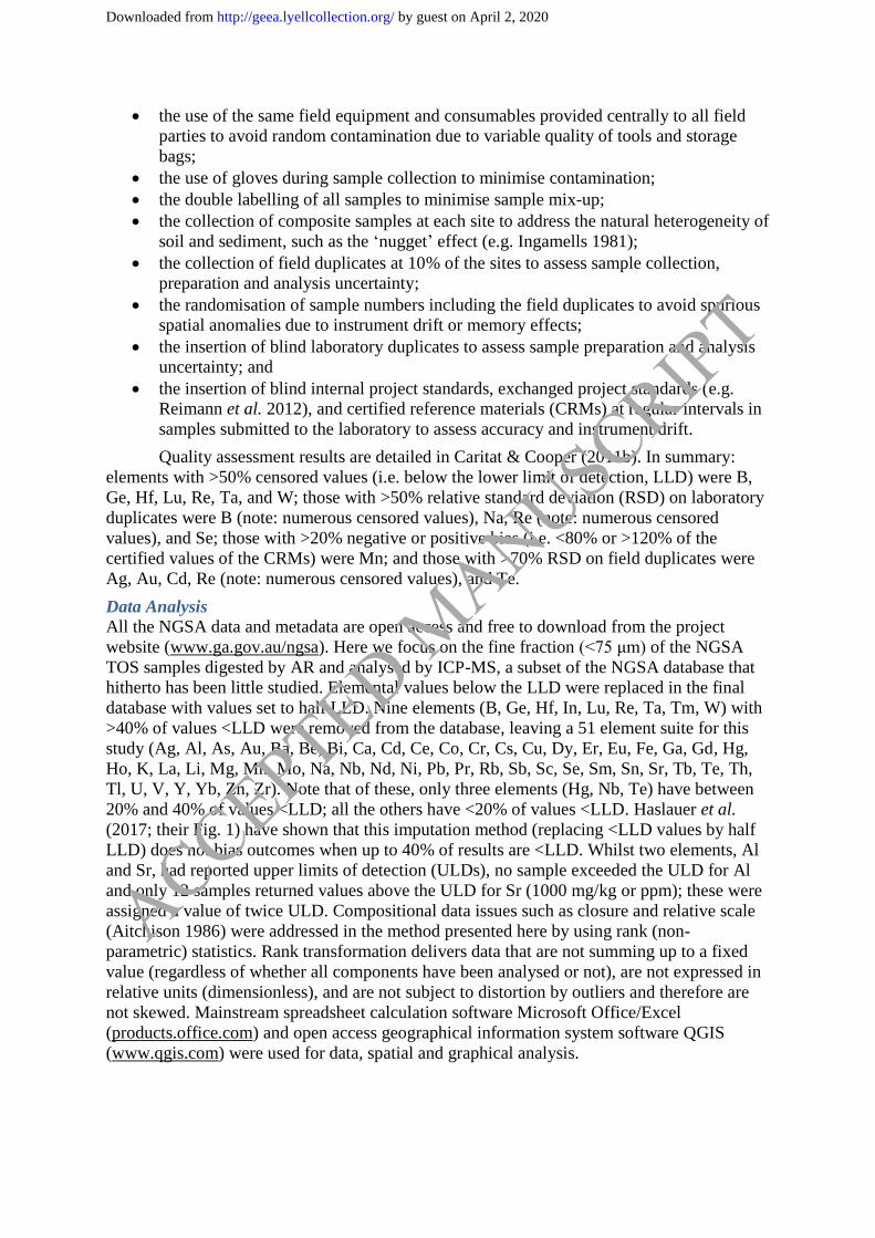
Spearman correlation and the geochemistry. Sample #2007191559 is a sample from a sub-
catchment of the main Swan-Avon drainage system near Beverley on the western side of the
Yilgarn Craton (see Fig. 1). The 1:250,000 scale geological sheet for Corrigin (Muhling &
Thom 1985a) indicates that the main rock types for this catchment are adamellite, gneiss and
migmatite (i.e. acid felsics) with minor (<5%) greenstone enclaves. The rankings in Figure 2
compare this sample with sample #2007190602 from near Merredin, also from the Swan-
Avon system, some 140 km to the northeast; the 1:250,000 geological sheet for Kellerberrin
(Muhling & Thom 1985b) indicates that the main rock types for this catchment are adamellite
(Kellerberrin batholith), adamellite with xenoliths of gneiss (i.e. acid felsics), and again with
less than 5% greenstone enclaves.
Despite there being some elements with different rankings in the two samples (e.g.
Ho, Yb, Zn, Cd) a high positive Spearman correlation coefficient (rs = 0.75) confirms that
these samples are geochemically very similar. Moreover, the linear regression on the ranks
has a slope close to unity (0.88) and a small intercept (84.9). It is concluded that this
geochemical fingerprint is diagnostic of ‘acid felsic’ geochemistry.
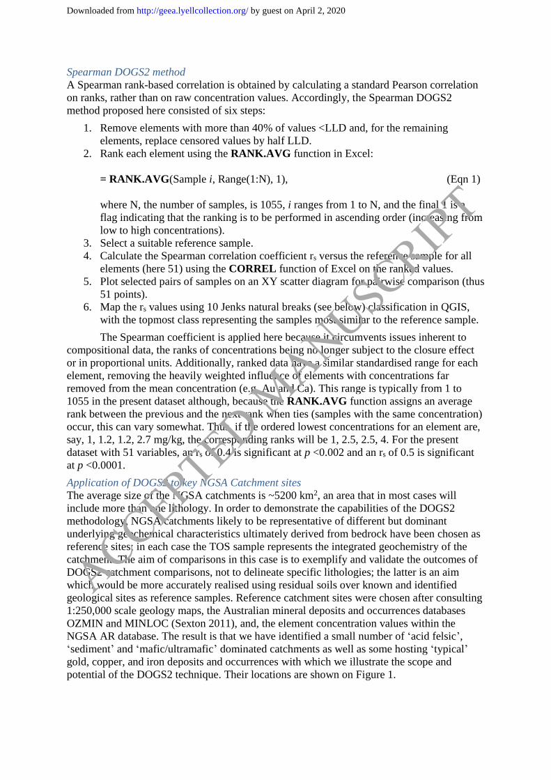
The ranking diagram for the TOS from the Beverley acid felsic catchment versus the
TOS selected from a mafic/ultramafic dominated catchment 100 km east of Kalgoorlie, is
very different (Fig. 3); the 1:250,000 geological sheet for Kurnalpi (Williams & Doepel
1971) suggests that the main rock units for the latter (#2007190484) are mainly from the
Mulgabbie (basic) and to a lesser extent Gindalbie and Gundockerta (turbidites, clastics, acid
volcanics) Formations.
ACCEPTED MANUSCRIPT
by guest on April 2, 2020http://geea.lyellcollection.org/Downloaded from
In this case the Spearman coefficient of correlation is negative (rs = -0.55). The linear
regression on the ranks has a negative slope (-0.81) and a large intercept (986). This is driven
by elements such as the REEs, U and Th, which are elevated in the granitoid-derived soil and
depleted in the greenstone-derived soil, and elements such as Au, Co, Cu, V, Se, Sr and Ca,
which have the opposite behaviour.
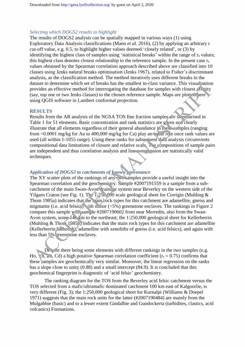
The ranking diagram between two soil samples from two predominantly
mafic/ultramafic catchments is shown in Figure 4. In this case the Kalgoorlie greenstone
(#2007190484) sample is compared to one further south in the Yilgarn Craton
(#2007190142) – from a catchment near lake Cowan 100 km east of Widgiemooltha. The
Widgiemooltha 1:250,000 geological sheet (Griffen & Hickman 1988) indicates that the main
rock types in this catchment are metamorphosed Archaean mafic and ultramafic rocks with
minor amounts of mafic/ultramafic material from Proterozoic dykes. The Erayinia granitoid
complex is marginal to the northeast.
The high positive Spearman correlation coefficient (rs = 0.66) between these two
samples together with the positive slope (0.72) and low intercept (160) of the linear
regression suggest a high degree of geochemical similarity. This is evident on the distribution
of elemental values on the XY scatter plot (Fig. 4) where elements such as Cr (labelled), Ni,
V, Sr, Se, Sc (unlabelled) in the top right of the diagram are all ranked relatively highly in
both samples. The REEs (within the ellipse in Fig. 4) are ranked relatively low in both of
these samples. It appears that the Spearman correlation coefficient of sample pairs has the
potential to provide a meaningful measure of the degree of geochemical similarity between
them.
Selection and use of reference samples
The selection of reference samples and the lithological and geochemical characteristics used
to select them are shown in Table 2; their locations are shown in Figure 1.
Selection of the first four references sample in Table 2 is facilitated by the fact that in
general catchments in the Yilgarn Craton are granite-dominated towards the west, and
greenstone-dominated towards the east, although it is likely that all catchments comprise
multiple/mixed lithologies. Column 4 of this table shows the concentrations of elements Ca,
Ce, Fe and Ni, which represent diagnostic characteristics. The various lithologies as
identified here appear to be represented by elevated concentrations of various elements in the
NGSA samples: acid felsics (Ce), mafics/ultramafics (Ni), marine carbonates (Ca), and
banded iron formation (Fe). The concentrations of Cu in catchment samples #2007190065
and #2007191289, which will be investigated in some detail below, are both elevated and
similar. Likewise values for Au in the Coolgardie and Ballarat catchment samples are similar
and higher than in other reference samples and were used in the selection of these catchments
as reference samples representative of catchments dominant in gold prospective lithologies
(‘auriferous geology’).
As with selection of the reference catchments, ‘identified samples’ (those highlighted
in red or orange on the accompanying maps) with closest affinity to the reference samples
identified by the DOGS2 process are subject to the same constraints imposed by the NGSA
sampling method (e.g. low sampling density, large catchments and ensuing likely mixed
lithological input, variable distance of sample site to bedrock outcrop/subcrop, weathering
history, etc.). Only a selected number of ‘identified samples’ with closest affinity to the
ACCEPTED MANUSCRIPT
by guest on April 2, 2020http://geea.lyellcollection.org/Downloaded from
reference sample (as determined by the Jenks breaks, see Methods section) are plotted in each
case for clarity.
From each reference sample a Spearman correlation coefficient for very other sample
in the NGSA database can be obtained. The correlation coefficients can be plotted as a single
independent variable located on a map by the sample coordinates (for further detail please
refer to the Methods section).
Degree of geochemical similarity map versus Beverley acid felsic catchment
The map with Beverley acid felsic catchment as the reference is shown in Figure 5. This map
highlights the top Jenks class many of which are located in the Yilgarn Craton; Cassidy et al.
(2013) discuss some of the reasons why more of the Yilgarn Craton catchments are not in this
top class. In addition, samples within the same class are located immediately southeast of the
Yilgarn Craton in the Proterozoic Albany-Fraser geological region and to the northwest of the
Craton where rivers draining the northern part of the Yilgarn Craton reach the Indian Ocean.
The quartz monzonites and adamellites of the Albany-Fraser geological region are thought to
be reworked Archean granitic material (www.ga.gov.au/provexplorer/province). The high
DOGS2 of a soil sample here supports this contention in at least one catchment. Other
samples with a similar high degree of similarity (rs >0.58) occur along northern Australian
coastlines and are related to acid felsics within catchments on Cape York Peninsula and in
Arnhem Land. A group of top Jenks class samples are shown in central Australia, and one is
also evident in western Victoria in the vicinity of the Grampian Mountains (Victoria Valley
granites), and another in southern South Australia near a granite quarry.
Degree of geochemical similarity map versus Kalgoorlie mafic/ultramafic
Figure 6 shows the map obtained when the Kalgoorlie mafic/ultramafic dominated catchment
is chosen as the reference sample for DOGS2 analysis. Proximal samples with DOGS2 in the
top Jenks class with respect to that reference sample are limited to the eastern goldfields
portion of the Yilgarn Craton. Only in this part of the Yilgarn Craton are catchments
dominated by mafic/ultramafic lithology. Three top Jenks class samples with high rs relative
to the Kalgoorlie mafic/ultramafic catchment sample also occur within the western Eucla
geological region near the boundary to the Albany-Fraser Belt. Recent Au discoveries in this
belt, such as the 6 million ounce Tropicana deposit (Doyle et al. 2013), occur in felsic
granulite thought to be the reworked margin of the Craton. A few catchments with a high
degree of similarity (rs >0.52) to the Kalgoorlie mafic/ultramafic dominated catchment also
occur in the Pilbara geological region. This similarity is probably based on geochemistry
resulting from a combination of predominantly mafic/ultramafic bedrock lithology and
regolith generated in arid to semi-arid terrain. Two catchments also with high similarity to
Kalgoorlie greenstone catchment occur in near coastal environments, on the Exmouth Gulf in
Western Australia and on the Nullarbor Coast in South Australia; these are more likely to be
marine carbonates (dolomites?) than locally derived greenstone, although the possibility of
transport of mafic/ultramafic material from the Pilbara and Yilgarn Cratons cannot be
excluded. Looking at the map of Australia highlighted with the highest Jenks class as shown
in Figure 6, it would appear that catchments with highest similarity to the Kalgoorlie
mafic/ultramafic dominated catchment are proximal to known mafic/ultramafic
outcrop/subcrop (Yilgarn, Pilbara, northeastern New South Wales, central eastern
Queensland, Tasmania, and Victoria).
ACCEPTED MANUSCRIPT
by guest on April 2, 2020http://geea.lyellcollection.org/Downloaded from
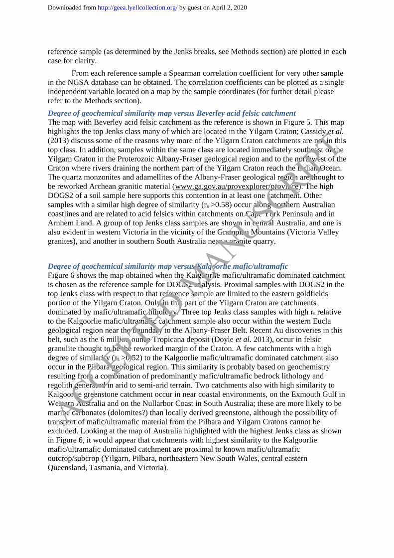
Degree of geochemical similarity map versus Nullarbor limestone
Both the NGSA MMI Ca map of Mann et al. (2012) and the modelling of Wilford et al.
(2015), among other evidence, indicate that carbonate terrain is common in the arid and semi-
arid areas of Australia. However, when a carbonate soil sample from the Nullarbor Plain
(#2007190159) is chosen as the reference, and the other NGSA AR samples correlated with
it, the distribution of the most highly correlated samples is more limited (Fig. 7). There is
however more than one type of carbonate (high Ca) terrain in Australia and it is likely that
multi-element geochemistry distinguishes them. All except four of the samples with the
highest DOGS2 relative to the Nullarbor Plain reference (Fig. 7) are within the Eucla
geological region (Blake & Kilgour 1998). The Nullarbor Plain in the Eucla geological region
may be the most extensive Miocene carbonate deposit described to date (O’Connell et al.
2012). The four other samples are either just outside the eastern boundary of the Eucla region
(just inside the Gawler geological region), or in the St Vincent and Pirie basins within the
Adelaide geological region, and the Murray Basin to the east of the Eucla region. The first of
these probably represents a mechanically transported geochemical signature. The three others
are in basins of more recent (Cenozoic) marine sediments that have progressively been
overlain in part by fluvial-lacustrine sediments (www.minerals.dmitre.sa.gov.au). Thus, it
appears that sample #2007190159 is a specific reference for marine limestone. For much of
the remainder of inland Australia soil samples have a (much) lower degree of similarity to
Nullarbor limestone sediments. Clearly a large number of secondary or regolith-derived
calcretes in Australia are distinct from these primary marine sediments when multi-element
geochemistry is considered.
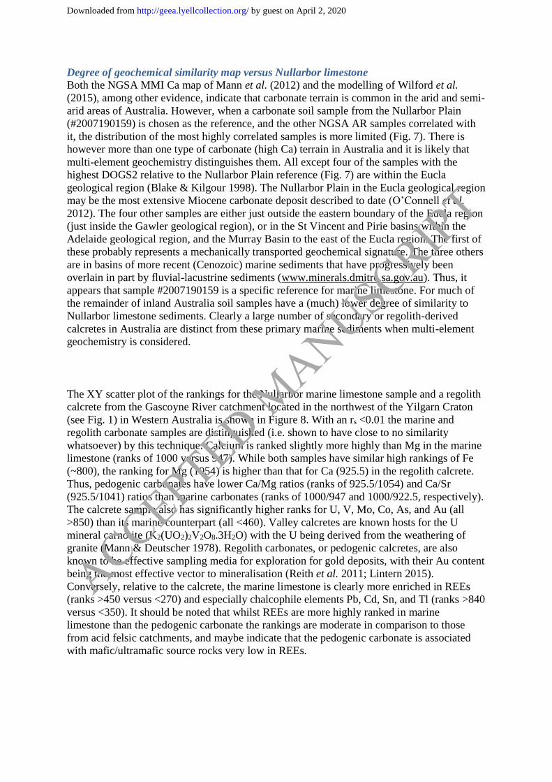
The XY scatter plot of the rankings for the Nullarbor marine limestone sample and a regolith
calcrete from the Gascoyne River catchment located in the northwest of the Yilgarn Craton
(see Fig. 1) in Western Australia is shown in Figure 8. With an rs <0.01 the marine and
regolith carbonate samples are distinguished (i.e. shown to have close to no similarity
whatsoever) by this technique. Calcium is ranked slightly more highly than Mg in the marine
limestone (ranks of 1000 versus 947). While both samples have similar high rankings of Fe
(~800), the ranking for Mg (1054) is higher than that for Ca (925.5) in the regolith calcrete.
Thus, pedogenic carbonates have lower Ca/Mg ratios (ranks of 925.5/1054) and Ca/Sr
(925.5/1041) ratios than marine carbonates (ranks of 1000/947 and 1000/922.5, respectively).
The calcrete sample also has significantly higher ranks for U, V, Mo, Co, As, and Au (all
>850) than its marine counterpart (all <460). Valley calcretes are known hosts for the U
mineral carnotite (K2(UO2)2V2O8.3H2O) with the U being derived from the weathering of
granite (Mann & Deutscher 1978). Regolith carbonates, or pedogenic calcretes, are also
known to be effective sampling media for exploration for gold deposits, with their Au content
being the most effective vector to mineralisation (Reith et al. 2011; Lintern 2015).
Conversely, relative to the calcrete, the marine limestone is clearly more enriched in REEs
(ranks >450 versus <270) and especially chalcophile elements Pb, Cd, Sn, and Tl (ranks >840
versus <350). It should be noted that whilst REEs are more highly ranked in marine
limestone than the pedogenic carbonate the rankings are moderate in comparison to those
from acid felsic catchments, and maybe indicate that the pedogenic carbonate is associated
with mafic/ultramafic source rocks very low in REEs.
ACCEPTED MANUSCRIPT
by guest on April 2, 2020http://geea.lyellcollection.org/Downloaded from
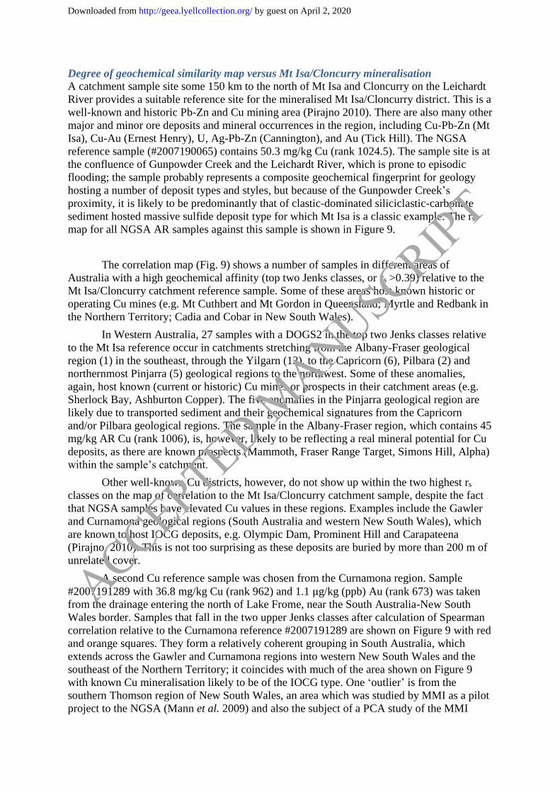
Degree of geochemical similarity map versus Mt Isa/Cloncurry mineralisation
A catchment sample site some 150 km to the north of Mt Isa and Cloncurry on the Leichardt
River provides a suitable reference site for the mineralised Mt Isa/Cloncurry district. This is a
well-known and historic Pb-Zn and Cu mining area (Pirajno 2010). There are also many other
major and minor ore deposits and mineral occurrences in the region, including Cu-Pb-Zn (Mt
Isa), Cu-Au (Ernest Henry), U, Ag-Pb-Zn (Cannington), and Au (Tick Hill). The NGSA
reference sample (#2007190065) contains 50.3 mg/kg Cu (rank 1024.5). The sample site is at
the confluence of Gunpowder Creek and the Leichardt River, which is prone to episodic
flooding; the sample probably represents a composite geochemical fingerprint for geology
hosting a number of deposit types and styles, but because of the Gunpowder Creek’s
proximity, it is likely to be predominantly that of clastic-dominated siliciclastic-carbonate
sediment hosted massive sulfide deposit type for which Mt Isa is a classic example. The rs
map for all NGSA AR samples against this sample is shown in Figure 9.
The correlation map (Fig. 9) shows a number of samples in different areas of
Australia with a high geochemical affinity (top two Jenks classes, or rs >0.39) relative to the
Mt Isa/Cloncurry catchment reference sample. Some of these areas host known historic or
operating Cu mines (e.g. Mt Cuthbert and Mt Gordon in Queensland; Myrtle and Redbank in
the Northern Territory; Cadia and Cobar in New South Wales).
In Western Australia, 27 samples with a DOGS2 in the top two Jenks classes relative
to the Mt Isa reference occur in catchments stretching from the Albany-Fraser geological
region (1) in the southeast, through the Yilgarn (13), to the Capricorn (6), Pilbara (2) and
northernmost Pinjarra (5) geological regions to the northwest. Some of these anomalies,
again, host known (current or historic) Cu mines or prospects in their catchment areas (e.g.
Sherlock Bay, Ashburton Copper). The five anomalies in the Pinjarra geological region are
likely due to transported sediment and their geochemical signatures from the Capricorn
and/or Pilbara geological regions. The sample in the Albany-Fraser region, which contains 45
mg/kg AR Cu (rank 1006), is, however, likely to be reflecting a real mineral potential for Cu
deposits, as there are known prospects (Mammoth, Fraser Range Target, Simons Hill, Alpha)
within the sample’s catchment.
Other well-known Cu districts, however, do not show up within the two highest rs
classes on the map of correlation to the Mt Isa/Cloncurry catchment sample, despite the fact
that NGSA samples have elevated Cu values in these regions. Examples include the Gawler
and Curnamona geological regions (South Australia and western New South Wales), which
are known to host IOCG deposits, e.g. Olympic Dam, Prominent Hill and Carapateena
(Pirajno, 2010). This is not too surprising as these deposits are buried by more than 200 m of
unrelated cover.
A second Cu reference sample was chosen from the Curnamona region. Sample
#2007191289 with 36.8 mg/kg Cu (rank 962) and 1.1 µg/kg (ppb) Au (rank 673) was taken
from the drainage entering the north of Lake Frome, near the South Australia-New South
Wales border. Samples that fall in the two upper Jenks classes after calculation of Spearman
correlation relative to the Curnamona reference #2007191289 are shown on Figure 9 with red
and orange squares. They form a relatively coherent grouping in South Australia, which
extends across the Gawler and Curnamona regions into western New South Wales and the
southeast of the Northern Territory; it coincides with much of the area shown on Figure 9
with known Cu mineralisation likely to be of the IOCG type. One ‘outlier’ is from the
southern Thomson region of New South Wales, an area which was studied by MMI as a pilot
project to the NGSA (Mann et al. 2009) and also the subject of a PCA study of the MMI
ACCEPTED MANUSCRIPT
by guest on April 2, 2020http://geea.lyellcollection.org/Downloaded from
NGSA data (Caritat et al. 2017), whilst two samples further north in the Eromanga region of
central Queensland are probably ‘false positives’. There is one sample from the Cu
mineralised Mt Isa/Cloncurry district of this type, and two samples from the coastal Pilbara
of Western Australia which overlap samples of the Mt Isa type; the latter are from outlet
sediments of the Sherlock and De Grey Rivers, catchments which host VMS style Cu-Zn-Pb
deposits.
The element ranking diagram for sample #2007190065 (Mt Isa type) versus
#2007191289 (Curnamona type) (not shown) indicates that Se, Mo, Bi, Mn, Gd and Co have
appreciably higher rankings in the former, whilst Na, Te, Sn, Sr, Al and Ca have higher
rankings in the latter reference.
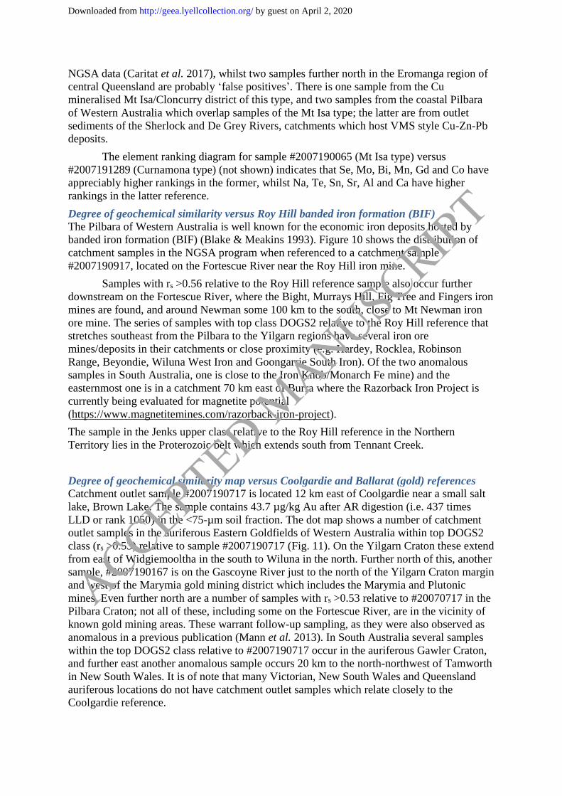
Degree of geochemical similarity versus Roy Hill banded iron formation (BIF)
The Pilbara of Western Australia is well known for the economic iron deposits hosted by
banded iron formation (BIF) (Blake & Meakins 1993). Figure 10 shows the distribution of
catchment samples in the NGSA program when referenced to a catchment sample
#2007190917, located on the Fortescue River near the Roy Hill iron mine.
Samples with rs >0.56 relative to the Roy Hill reference sample also occur further
downstream on the Fortescue River, where the Bight, Murrays Hill, Fig Tree and Fingers iron
mines are found, and around Newman some 100 km to the south, close to Mt Newman iron
ore mine. The series of samples with top class DOGS2 relative to the Roy Hill reference that
stretches southeast from the Pilbara to the Yilgarn regions have several iron ore
mines/deposits in their catchments or close proximity (e.g. Hardey, Rocklea, Robinson
Range, Beyondie, Wiluna West Iron and Goongarrie South Iron). Of the two anomalous
samples in South Australia, one is close to the Iron Knob/Monarch Fe mine) and the
easternmost one is in a catchment 70 km east of Burra where the Razorback Iron Project is
currently being evaluated for magnetite potential
(https://www.magnetitemines.com/razorback-iron-project).
The sample in the Jenks upper class relative to the Roy Hill reference in the Northern
Territory lies in the Proterozoic belt which extends south from Tennant Creek.
Degree of geochemical similarity map versus Coolgardie and Ballarat (gold) references
Catchment outlet sample #2007190717 is located 12 km east of Coolgardie near a small salt
lake, Brown Lake. The sample contains 43.7 µg/kg Au after AR digestion (i.e. 437 times
LLD or rank 1050) in the <75-µm soil fraction. The dot map shows a number of catchment
outlet samples in the auriferous Eastern Goldfields of Western Australia within top DOGS2
class (rs >0.53) relative to sample #2007190717 (Fig. 11). On the Yilgarn Craton these extend
from east of Widgiemooltha in the south to Wiluna in the north. Further north of this, another
sample, #2007190167 is on the Gascoyne River just to the north of the Yilgarn Craton margin
and west of the Marymia gold mining district which includes the Marymia and Plutonic
mines. Even further north are a number of samples with rs >0.53 relative to #20070717 in the
Pilbara Craton; not all of these, including some on the Fortescue River, are in the vicinity of
known gold mining areas. These warrant follow-up sampling, as they were also observed as
anomalous in a previous publication (Mann et al. 2013). In South Australia several samples
within the top DOGS2 class relative to #2007190717 occur in the auriferous Gawler Craton,
and further east another anomalous sample occurs 20 km to the north-northwest of Tamworth
in New South Wales. It is of note that many Victorian, New South Wales and Queensland
auriferous locations do not have catchment outlet samples which relate closely to the
Coolgardie reference.
ACCEPTED MANUSCRIPT
by guest on April 2, 2020http://geea.lyellcollection.org/Downloaded from
The red squares in Figure 11 show NGSA samples with top Jenks class similarity to
another type of gold deposit, for which the NGSA sample #2007190042 near Ballarat, in
Victoria, was chosen to be the reference. This sample contains 18.4 µg/kg Au after AR
digestion (rank 1039) in the <75-µm soil fraction. The Jenks upper class cohort versus this
reference produces samples in most areas in the eastern states shown as auriferous, up to and
including the Palmer River goldfield on the Cape York Peninsula. The ranking diagram for
the Coolgardie reference (#2007190717) versus Ballarat reference (#2007190042) shows that
the Coolgardie reference has very high rankings for many elements such as Cd, Cu, Zn, Te,
Sc, Ga, Al relative to the Ballarat reference, which in turn has higher rankings for elements
such as Nb, Ce, Nd, Sm, Gd, Pb and Hg. It is clear that these reference samples pick out a
different set of NGSA samples, showing that not only is the high Au content important but
the complete geochemical fingerprint allows targeting of very specific conditions, such as
comparing Archaean greenstone versus Eastern Australian (younger sediment-related) style
Au mineralisation. This approach, which considers significant Au value and other associated
elements, could be important for outlining areas prospective for Au in covered terrain.
DISCUSSION
It is fundamental to this method that Spearman correlation coefficients differ appreciably in
soils derived from different lithologies. For this to occur the concentrations subsequent to AR
digestion and ICP-MS analysis of many if not most elements have to vary sufficiently
between samples. It is also important that in digestions of similar soils, the ranking of
elements digested remains similar. In Table 3 the rankings of some key elements in soils from
catchments with different dominant lithologies are presented. Whilst the similarity of
individual element rankings from catchments with similar lithologies (top six rows) evidently
is conducive to the high DOGS2 between respective pairs, it is instructive to also examine the
geochemical makeup of samples representing mineralised areas (bottom five rows).
Felsic igneous bedrock, represented by the granite-derived soil samples in Table 3,
have their rankings dominated by REEs Ce, La and Yb, followed by Al, K, Mg and Ag; Ba,
Fe and Cu have the lowest ranks. Mafic lithologies (greenstone-derived samples) have their
rankings dominated by Ca, Ni, Mg, Fe, Cu and Au; Ag, Ce and Yb have the lowest ranks.
Carbonate-derived soils have different geochemical signatures depending on their origin:
marine limestone has high ranks for Ca, K, Mg and Al, with low Au, La and Ce; regolith
carbonate has high ranks for Mg, Ni, Cu and Ca, with low La, Ce and Yb. The change in
relative ranking order between Ca and Mg between marine (Ca>Mg) and pedogenic (Mg>Ca)
carbonates noted here is in accord with the findings of Wolff et al. (2017), indicating that
practical geochemical indicators derived from raw geochemical concentrations can be
preserved when converting to rank statistics The differences highlighted in Table 3 allow for
a practical differentiation of marine versus pedogenic carbonates: the latter will likely have
higher Mg, Ni, Cu and Au and lower Yb, La, Ce and Ag rankings (and concentrations) than
their marine counterparts. Thus elevated Mg/REE, Ni/REE, Mg/Ca, Cu/Ag or Au/Ag rank
ratios in carbonate-derived soils will tend to indicate a pedogenic (calcrete) origin.
The Mt Isa type Cu mineralisation style is indicated by a geochemical fingerprint with
elevated Cu, Fe, La and Ce ranks, and depressed Al, Ca and Mg ranks. The Curnamona style
of Cu mineralisation, while still having an elevated Cu rank, also has high rankings for Ca, K
and Fe, and low ranks for Yb and Ag. Banded Iron Formation mineralisation typical of the
Pilbara region is diagnosed by soils with raised Cu, Fe, Ni and Ag ranks accompanied by low
Ce, Au, Ca and La ranks. It appears that soils from auriferous regions in general have high
ACCEPTED MANUSCRIPT
by guest on April 2, 2020http://geea.lyellcollection.org/Downloaded from
Au and Ni ranks, and intermediate to low Ba, Ca and Yb. ‘Archean Yilgarn’ style Au
mineralisation differs from ‘Paleozoic Eastern Australian’ style Au mineralisation by its
higher Cu, Al, Ca and K ranks and its lower La, Ce, Au and Ag ranks.
Sensitivity analysis shows that this outcome is relatively independent of values of Au
and Cu in the samples; in column 3 of Table 4 the rs values for a number of reference
samples, including the Coolgardie (#2007190717) and Ballarat samples (#2007190042) with
Au and Cu removed from the Spearman rs calculation are compared to those in column 2
where all 51 elements are included. The changes in all cases are minimal – commodity
elements Au and Cu have only a minor effect on the Spearman calculation. This extends to
elements such as Mg and Ni, which it might be thought have an important effect on
comparison of catchments with greenstone lithology (#2007190484 vs #2007190142) and Ca
and Fe, the major elements in many aqua regia digests. The sensitivity analysis suggests the
method is extremely robust and relies on the contribution from a large number of elements to
generate similarities (or differences).
It is only when the 12 rare earth elements (lanthanides) are removed, in addition to
Au, Cu, Mg, Ni, Ca and Fe that some reference comparisons (column 6 of Table 4) show
differences in rs of >0.1 compared to the values in column 2. The Spearman rs shown in red in
Table 4 between a predominantly granitoid catchment (#2007191559) and a greenstone
dominated one (#2007190484) decreases i.e. the samples appear more similar with removal
of the REEs indicating their importance in distinguishing acid felsic from mafic/ultramafic
lithologies. Removal of the REEs however decreases the high rs between granitoid samples
#2007191559 and #2007190602 illustrating that elements other than the REEs are also
involved in the differences between these two granitoid dominated catchments. Similar
conclusions can be drawn in the case of the marine carbonate and pedogenic calcrete
comparison (#2007190159 vs #2007190881) and the overall geology of the two Cu
prospective catchments (#2007190065 vs #2007191289).
Comparison of the outcomes from this study with those from the previous DOGS
(Mann et al. 2016) study is difficult to do in detail because (a) the analytical technique is
different (AR versus MMI), (b) the DOGS2 technique in this study utilises Spearman
correlation (ranking) of analytical data rather than a Pearson correlation of log-transformed
data, and (c) the method of assessment of ‘upper class’ uses Jenks breaks rather than upper
two percentiles. Notwithstanding this, the outcomes share similarities; many of the identified
(‘upper class’) samples from the present study are within the same geological regions that
contained the upper two percentiles of MMI samples (Mann et al. 2016). One important
difference however is that the Spearman r (rs) values are in all cases lower than the equivalent
Pearson r values; this is almost certainly due to the ranking procedure. In some cases the
Spearman ranking coefficient is negative (e.g. granite versus greenstone). This increased
spread of correlation coefficient values is an advantage in sample comparisons, making the
technique more sensitive.
We tested the results of a clr transformation compared to our DOGS2 rank-based
method. The two approaches give similar results, with mostly the same NGSA samples being
identified as the most similar to a reference sample (e.g. #2007191559, Fig. 5), and the
resulting maps are consequently also highly correlated. The rank-based approach however
appears to be much more discriminating, giving a range of Spearman correlation coefficients
(rs) for the NGSA dataset of -0.8 to +0.9, whereas the correlations of all samples against the
same reference sample based on clr-transformed data only varies from +0.73 to +0.98. In
other words, catchments with a lithology that is opposite (e.g. mafic) to the reference sample
ACCEPTED MANUSCRIPT
by guest on April 2, 2020http://geea.lyellcollection.org/Downloaded from
(e.g. felsic) have a clear (and expected) negative rs in the DOGS2 method, yet are still shown
to have a high positive correlation coefficient with the clr method (0.73, significant at
p<<0.01 for this dataset). The resulting maps show very much the same regions being
highlighted as similar to the reference, but the contrast is much better with DOGS2.
Alternative and perhaps more conventional methods of measuring ‘closeness’ of
geochemical data are through the Euclidean or Aitchison distances (with distance decreasing
as similarity increases). Preliminary comparison with the DOGS2 method suggests that for
most reference samples tested the results are generally compatible and yield similar spatial
patterns on maps; in a few cases, however, results appear poorly correlated between DOGS2
and the inverse of distance. Whilst it is not known which method is necessarily correct and
further investigation is required to understand implications, the DOGS2 method provides a
simple, robust and tested (herein and in Mann et al. 2016) method of quantifying
geochemical similarity in large datasets.
CONCLUSIONS
Aqua regia (AR) data from the National Geochemical Survey of Australia (NGSA) database
have been used to assess the degree of geochemical similarity (DOGS2) of catchments based
on catchment outlet soil samples and Spearman (rank-based) correlation coefficients (rs);
reference samples from catchments with a dominant geochemistry have been used to produce
correlation-based maps that show the distribution of the DOGS2 of all catchments in the
NGSA AR dataset relative to each reference sample. Reference catchment sites dominant in
acid felsic, mafic/ultramafic and carbonate (both marine and calcrete) lithologies on the one
hand, and banded iron formation, copper and gold mineralisation on the other hand, have
been chosen to demonstrate the method and to provide diagnostic geochemical information. It
is interesting that in each case some of the samples identified to have highest similarities to
the reference are located other than proximal to the reference, i.e. Australia-wide, in other
geological provinces.
Based on the NGSA AR sample set, proposed criteria for a meaningfully high
DOGS2 between pairs of samples are: rs >0.4 (significant at p <0.002), linear regression
slopes >0.7 and intercepts <200. Sample pairs that show no particular relationship to one
another may have rs ~0, linear regression slopes ~0 and variable intercepts. Strongly
antithetic relationships, such as felsic- versus mafic-derived soils, will have negative rs,
negative linear regression slope values and variable intercepts.
Utilisation of all significant (not overly censored) elements in the analysed multi-
element suite ensures that the method is objective by taking the full compositional fingerprint
into account. This comparative multi-element method provides information for geochemical
interpretation complementary to that provided by single element interrogation of databases.
Preliminary applications are suggested to be: differentiation of soils derived from various
source lithologies, diagnostic distinction of a marine versus terrestrial origin of carbonate in
soil, and a first order mineral prospectivity tool. The approach presented here is an
improvement on a previous development of DOGS, which ensures the analysis is appropriate
for compositional data. The new method of determining the degree of geochemical similarity,
DOGS2, could find wide application in the fields of sediment provenance, archaeology,
agriculture, environmental investigations, geological mapping, digital soil mapping, resource
evaluation, geochemical exploration, and forensic geochemistry.
ACKNOWLEDGEMENTS
The NGSA project was part of the Australian Government’s Onshore Energy Security
Program 2006–2011, from which funding support is gratefully acknowledged. NGSA was led
ACCEPTED MANUSCRIPT
by guest on April 2, 2020http://geea.lyellcollection.org/Downloaded from
and managed by Geoscience Australia and carried out in collaboration with the geological
surveys of every State and the Northern Territory under National Geoscience Agreements.
The authors acknowledge and thank all landowners for granting access to the sampling sites
and all those who took part in sample collection. The sample preparation and analysis team at
Geoscience Australia and analytical staff at Actlab’s Perth laboratories are all thanked for
their contributions. Constructive reviews of earlier versions of this manuscript were provided
by Andrew McPherson and David Champion (Geoscience Australia), for which we are
thankful. We are grateful also to Graeme Bonham-Carter for taking the time to scrutinise the
DOGS2 method and provide feedback on how it compares to the measure of “distance”
between compositional vectors. Paul Morris and an anonymous journal reviewer are thanked
for their helpful advice and comments on the original manuscript. PdC publishes with
permission from the Chief Executive Officer, Geoscience Australia.
REFERENCES
AITCHISON, J. 1986. The Statistical Analysis of Compositional Data. Chapman & Hall.
Reprinted in 2003 with additional material by The Blackburn Press.
BLAKE, D., KILGOUR, B. 1998. Geological Regions of Australia 1:5,000,000 scale.
Geoscience Australia. Available at: http://www.ga.gov.au/metadata-
gateway/metadata/record/gcat_a05f7892-b237-7506-e044-
00144fdd4fa6/Geological+Regions+of+Australia%2C+1%3A5+000+000+scale
BLAKE, S., HENRY, T., MURRAY, J., FLOOD, R., MULLER, M.R., JONES, A.G.,
RATH, V. 2016. Compositional multivariate statistical analysis of thermal groundwater
provenance: a hydrogeochemical case study from Ireland. Applied Geochemistry, 75, 171-
188. doi: 10.1016/j.apgeochem.2016.05.008.
BLAKE, T.S., MEAKINS, A.L., (Eds) 1993. Archaean and Early Proterozoic Geology of the
Pilbara Region, Western Australia. Precambrian Research, 60, 1-359.
BOWEN, A.M., CAVEN, E.A. 2013. Forensic provenance investigations of soil and
sediment samples. In: PIRRIE, D., RUFFELL, A., DAWSON, L.A. (eds), Environmental and
Criminal Geoforensics. Geological Society, London, Special Publications, 384, 9-25. doi:
10.1144/SP384.4.
CARITAT, P. de, COOPER, M. 2011a. National Geochemical Survey of Australia: The
Geochemical Atlas of Australia. Geoscience Australia Record, 2011/20 (2 Volumes), 557 pp.
Available at: http://www.ga.gov.au/metadata-gateway/metadata/record/gcat_71973
CARITAT, P. de, COOPER, M. 2011b. National Geochemical Survey of Australia: Data
Quality Assessment. Geoscience Australia Record, 2011/21 (2 Volumes), 478 pp. Available
at: http://www.ga.gov.au/metadata-gateway/metadata/record/gcat_71971
CARITAT, P. de, COOPER, M. 2016. A continental-scale geochemical atlas for resource
exploration and environmental management: the National Geochemical Survey of Australia.
Geochemistry: Exploration, Environment, Analysis, 16, 3-13. doi: 10.1144/geochem2014-
322.
CARITAT, P. de, GRUNSKY, E.C. 2013. Defining element associations and inferring
geological processes from total element concentrations in Australian catchment outlet
sediments: multivariate analysis of continental-scale geochemical data. Applied
Geochemistry, 33, 104-126. doi: 10.1016/j.apgeochem.2013.02.005.
CARITAT, P. de, COOPER, M., WILFORD, J. 2011. The pH of Australian soils: field
results from a national survey. Soil Research, 49, 173-182. doi: 10.1071/SR10121.
ACCEPTED MANUSCRIPT
by guest on April 2, 2020http://geea.lyellcollection.org/Downloaded from
CARITAT, P. de, COOPER, M., LECH, M., McPHERSON, A., THUN, C. 2009. National
Geochemical Survey of Australia: Sample Preparation Manual. Geoscience Australia Record
2009/08, 28 p. Available at: http://www.ga.gov.au/metadata-
gateway/metadata/record/gcat_68657
CARITAT, P. de, COOPER, M., PAPPAS, W., THUN, C., WEBBER, E. 2010. National
Geochemical Survey of Australia: Analytical Methods Manual. Geoscience Australia Record
2010/15, 22 p. Available at: http://www.ga.gov.au/metadata-
gateway/metadata/record/gcat_70369
CARITAT, P. de, LECH, M.E., McPHERSON, A. 2008. Geochemical mapping “down
under”: selected results from pilot projects and strategy outline for the National Geochemical
Survey of Australia. Geochemistry: Exploration, Environment, Analysis, 8, 301-312. doi:
10.1144/1467-7873/08-178.
CARITAT, P. de, MAIN, P., GRUNSKY, E., MANN, A. 2017. Recognition of geochemical
footprints of mineral systems in the regolith at regional to continental scales. Australian
Journal of Earth Sciences, published online. doi: 10.1080/08120099.2017.1259184.
CASSIDY, K.F., CHAMPION, D.C., KRAPEZ, B., BARLEY, M.E., BROWN, S.J.A.,
BLEWTT, R.S., GROENWALD, B.B., TYLER, I.M. 2006. A revised geological framework
for the Yilgarn Craton, Western Australia. Western Australian Geological Survey Record,
2006/8. Available at https://dmpbookshop.eruditetechnologies.com.au
CHURCH, S.E., MOSIER, E.L., MOTOOKA, J.M. 1987. Mineralogical basis for the
interpretation of multi-element (ICP-AES), oxalic acid, and aqua regia partial digestions of
stream sediments for reconnaissance exploration geochemistry. Journal of Geochemical
Exploration, 29, 207-233. doi: 10.1016/0375-6742(87)90078-1.
DOYLE, M., SAVAGE, J., BLENKINSOP, T.G., CRAWFORD, A., McNAUGHTON, N.
2013. Tropicana – Unravelling the complexity of a +6 million ounce gold deposit hosted in
granulite facies metamorphic rocks. In: World Gold 2013. Australian Institute of Mining and
Metallurgy, Brisbane, 87-93.
FENG, J.-L., HU, Z.-G., JU, J.-T., ZHU, L.-P. 2011. Variations in trace element (including
rare earth element) concentrations with grain sizes in loess and their implications for tracing
the provenance of eolian deposits. Quaternary International, 236, 116-126. doi:
10.1016/j.quaint.2010.04.024.
FREI, R., FREI, K.M. 2013. The geographic distribution of Sr isotopes from surface waters
and soil extracts over the island of Bornholm (Denmark) - A base for provenance studies in
archeology and agriculture. Applied Geochemistry, 38, 147-160. doi:
10.1016/j.apgeochem.2013.09.007.
GAUDINO, S., GALAS, C., BELLI, M., BARBIZZI, S., ZORZI, P. de, JAĆIMOVIĆ, R.,
JERAN, Z., PATI, A., SANSONE, U. 2007. The role of different soil sample digestion
methods on trace elements analysis: a comparison of ICP-MS and INAA measurement
results. Accreditation and Quality Assurance, 12, 84-93. doi: 10.1007/s00769-006-0238-1.
GRESHAM, J.J., LOFTUS-HILLS, G.D. 1981. The geology of the Kambalda nickel field,
Western Australia. Economic Geology, 76, 1373-1416. doi: 10.2113/gsecongeo.76.6.1373.
GRIFFIN, T.J., HICKMAN, A.H. 1988. Widgiemooltha 1:250,000 geological sheet, Western
Australia. Geological Survey of Western Australia.
GRUNSKY, E. 2010. The interpretation of geochemical survey data. Geochemistry:
Exploration, Environment, Analysis, 10, 27-74. doi: 10.1144/1467-7873/09-210.
ACCEPTED MANUSCRIPT
by guest on April 2, 2020http://geea.lyellcollection.org/Downloaded from
HASLAUER, C.P., MEYER, J.R., BÁRDOSSY, A., PARKER, B.L. 2017. Estimating a
representative value and proportion of true zeros for censored analytical data with
applications to contaminated site assessment. Environmental Science & Technology, 51,
7502-7510. doi: 10.1021/acs.est.6b05385.
HEBERLEIN, D.R. 2010. An Assessment of Soil Geochemical Methods for Detecting
Copper-Gold Porphyry Mineralization through Quaternary Glaciofluvial Sediments at the
WBX-MBX and 66 Zones, Mt Milligan, North-Central British Columbia. Geoscience British
Columbia Report, 2010-08, 68 p.
INGAMELLS, C.O. 1981. Evaluation of skewed exploration data – the nugget effect.
Geochimica et Cosmochimica Acta, 45, 1209-1216. doi: 10.1016/0016-7037(81)90144-7.
ISO (International Organization for Standardization) 2016. Soil Quality — Extraction of
Trace Elements Soluble in Aqua Regia. International Standard ISO 11466:1995 (reviewed
and confirmed in 2016), 6 p.
JENKS, G.F. 1967. The data model concept in statistical mapping. International Yearbook of
Cartography, 7, 186-190.
KEEGAN, E., RICHTER, S., KELLY, I., WONG, H., GADD, P., KUEHN, H., ALONSO-
MUNOZ, A. 2008. The provenance of Australian uranium ore concentrates by elemental and
isotopic analysis. Applied Geochemistry, 23, 765-777. doi:
10.1016/j.apgeochem.2007.12.004.
KISSER, M.I. 2005. Digestion of Solid Matrices, Part 1: Digestion with Aqua Regia - Report
of Evaluation Study. Horizontal 18, Report, 38 p. Available at:
https://www.ecn.nl/docs/society/horizontal/Digestion_report_Aqua_regia.pdf
LECH, M.E., CARITAT, P. de, McPHERSON, A.A. 2007. National Geochemical Survey of
Australia: Field Manual. Geoscience Australia Record, 2007/08, 53 p. Available at:
http://www.ga.gov.au/metadata-gateway/metadata/record/gcat_65234
LINTERN, M.J. 2015. The association of gold with calcrete. Ore Geology Reviews, 66, 132-
199. doi: 10.1016/j.oregeorev.2014.10.029.
MANN, A., DEUTSCHER, R. 1978. Genesis principles for the precipitation of carnotite in
calcrete drainages in Western Australia. Economic Geology, 73, 1724-1737. doi:
10.2113/gsecongeo.73.8.1724.
MANN, A. 2010. Strong versus weak digestions: ligand-based soil extraction geochemistry.
Geochemistry: Exploration, Environment, Analysis, 10, 17-26. doi: 10.1144/1467-7873/09-
216.
MANN, A., CARITAT, P. de, GREENFIELD, J. 2009. Geochemistry of catchment outlet
sediments: evaluation of Mobile Metal Ion Analyses from the Thomson Region, New South
Wales, Australia. Proceedings of the 24th International Applied Geochemistry Symposium,
Fredericton, New Brunswick, Canada, Volume II, 759-762.
MANN, A., CARITAT, P. de, PRINCE, P. 2012. Bioavailability of nutrients in Australia
from Mobile Metal Ion analysis of catchment outlet samples: continental scale patterns and
processes. Geochemistry: Exploration, Environment, Analysis, 12, 277-292. doi:
10.1144/geochem2011-090.
MANN, A., CARITAT, P. de, SYLVESTER, G. 2016. Degree of Geochemical Similarity
(DOGS): a simple statistical method to quantify and map affinity between samples from
multi-element geochemical data sets. Australian Journal of Earth Science, 63, 111-122. doi:
10.1080/08120099.2016.1130744.
ACCEPTED MANUSCRIPT
by guest on April 2, 2020http://geea.lyellcollection.org/Downloaded from
MANN, A., DAVIDSON, A., CARITAT, P. de 2013. High resolution soil geochemistry for
gold exploration at the continental, regional and prospect scale. In: World Gold 2013,
Australian Institute of Mining and Metallurgy, Brisbane, 167-174.
MANN, A., REIMANN, C., CARITAT, P. de, TURNER, N., BURKE, M., GEMAS
PROJECT TEAM 2015. Mobile Metal Ion analysis of European agricultural soils:
bioavailability, weathering, geogenic patterns and anthropogenic anomalies. Geochemistry:
Exploration, Environment, Analysis, 15, 99-112. doi: 10.1144/geochem2014-279.
MANN, A.W., BIRRELL, R., MANN, A.T., HUMPHREYS, D., PERDRIX J. 1998.
Application of the Mobile Metal Ion technique to routine geochemical exploration. Journal of
Geochemical Exploration, 61, 87-102. doi: 10.1016/S0375-6742(97)00037-X.
McBRATNEY, A.B., MENDONÇA SANTOS, M.L., MINASNY, B. 2003. On digital soil
mapping. Geoderma, 117, 3-52. doi: 10.1016/S0016-7061(03)00223-4.
MUHLING, P.C., THOM, R. 1985a. Corrigin 1:250,000 geological sheet, Western Australia.
Geological Survey of Western Australia.
MUHLING, P.C., THOM, R. 1985b. Kellerberrin 1:250,000 geological sheet, Western
Australia. Geological Survey of Western Australia.
O’CONNELL, L.G., JAMES, N.P., BONE, Y. 2012. The Miocene Nullarbor Limestone,
southern Australia; deposition on a vast subtropical epeiric platform. Sedimentary Geology,
253-254, 1-16. doi: 10.1016/j.sedgeo.2011.12.002.
PIRAJNO, F. 2010. Hydrothermal Processes and Mineral Systems. Springer Science and
Business Media B.V. Dordrecht, The Netherlands, 1250 p.
REACH (Registration, Evaluation, Authorisation and Restriction of Chemicals) 2008.
Guidance on information requirements and chemical safety assessment - Appendix R.7.13-2:
Environmental risk assessment for metals and metal compounds. Guidance for the
implementation of REACH, European Chemicals Agency (ECHA), 74 p. Available at:
http://guidance.echa.europa.eu/docs/guidance_document/information_requirements_r7_13_2
_en.pdf
REID, A., KEELING, J.L., BELOUSOVA, E.A. 2013. Hf isotopic investigation into the
provenance of zircons in heavy mineral sands of the Eucla Basin. MESA Journal (Resources
and Energy Group, Department of Manufacturing, Innovation, Trade, Resources and Energy,
South Australia), 68, 17-24.
REIMANN C., FILZMOSER, P., GARRETT, R., DUTTER, R. 2008. Statistical Analysis
Explained: Applied Environmental Statistics with R. J. Wiley & Sons, Chichester, 424 p.
REIMANN, C., CARITAT, P. de, GEMAS Project Team, NGSA Project Team 2012. New
soil composition data for Europe and Australia: demonstrating comparability, identifying
continental-scale processes and learning lessons for global geochemical mapping. Science of
the Total Environment, 416, 239-252. doi: 10.1016/j.scitotenv.2011.11.019.
REITH, F., ETSCHMANN, B., DART, R.C., BREWE, D.L., VOGT, S., SCHMIDT
MUMM, A., BRUGGER, J. 2011. Distribution and speciation of gold in biogenic and
abiogenic calcium carbonates - Implications for the formation of gold anomalous calcrete.
Geochimica et Cosmochimica Acta, 75, 1942-1956. doi: 10.1016/j.gca.2011.01.014.
RUBESKA, I., EBARVIA, B., MACALALAD, E., RAVIS, D., ROQUE, N. 1987. Multi-
element pre-concentration by solvent extraction compatible with an aqua regia digestion for
geochemical exploration samples. Analyst, 112, 27-29. doi: 10.1039/AN9871200027.
ACCEPTED MANUSCRIPT
by guest on April 2, 2020http://geea.lyellcollection.org/Downloaded from
SCHEIB, A.J. 2013. The National Geochemical Survey of Australia – Selected
Interpretations for Western Australia. Geological Survey of Western Australia Record,
2013/4. Available at https://dmpbookshop.eruditetechnologies.com.au
SEXTON, M. 2011. Australian Mineral Occurrences Collection. Geoscience Australia.
Available at: https://ecat.ga.gov.au/geonetwork/srv/eng/search#!b3dc063b-7f35-24b7-e044-
00144fdd4fa6
SHAW, R.D., YEATES, A.N., PALFREYMAN, W.D., DOUTCH, H.F. 2000. Surface
Geology of Australia 1:5 Million Scale Dataset. Geoscience Australia. Available at:
https://ecat.ga.gov.au/geonetwork/srv/eng/search#!a05f7892-b444-7506-e044-00144fdd4fa6
SYLVESTER, G.C., MANN, A.W., COOK, S.R., WILSON, C.A. 2017. MMI partial
extraction geochemistry for the resolution of anthropogenic activities across the
archaeological Roman town of Calleva Atrebatum. Geochemistry: Exploration, Environment,
Analysis, published online. doi: 10.1144/geochem2017-009.
TARAŠKEVIČIUS, R., ZINKUTĖ, R., STAKĖNIENĖ, R., RADAVIČIUS, M. 2013. Case
study of the relationship between aqua regia and real total contents of harmful trace elements
in some European soils. Journal of Chemistry, Article ID 678140, 15 p. doi:
10.1155/2013/678140.
TIGHE, M., LOCKWOOD, P., WILSON, S., LISLE, L. 2004. Comparison of digestion
methods for ICP-OES analysis of a wide range of analytes in heavy metal contaminated soil
samples with specific reference to arsenic and antimony. Communications in Soil Science
and Plant Analysis, 35, 1369-1385. doi: 10.1081/CSS-120037552.
TUKEY, J. 1977. Exploratory Data Analysis. Addison-Wesley, Reading, MA, 506 pp.
USEPA (United States Environmental Protection Agency) 2015. Test Methods for Evaluating
Solid Waste, Physical/Chemical Methods, EPA publication SW‐ 846, Third Edition, Final
Updates I (1993), II (1995), IIA (1994), IIB (1995), III (1997), IIIA (1999), IIIB (2005), IV
(2008), and V (2015). Washington, DC, USA. Available at: https://www.epa.gov/hw-
sw846/sw-846-compendium
WELTE, G.J., EYNATTEN, H. von 2004. Quantitative provenance analysis of sediments:
review and outlook. Sedimentary Geology, 171, 1-11. doi: 10.1016/j.sedgeo.2004.05.007.
WILFORD, J., CARITAT, P. de, BUI, E. 2015. Modelling the abundance of soil calcium
carbonate across Australia using geochemical survey data and environmental predictors.
Geoderma, 259-260, 81-92. doi: 10.1016/j.geoderma.2015.05.003.
WOLFF, K., TIDDY, C., GILES, D., HILL, S.M., GORDON, G. 2017. Distinguishing
pedogenic carbonates from weathered marine carbonates on the Yorke Peninsula, South
Australia: implications for mineral exploration. Journal of Geochemical Exploration, 181, 81-
98. doi: 10.1016/j.gexplo.2017.06.019.
ZHANG, S., YANG, D., LI, F., CHEN, H., HUANG, B., ZOU, D., YANG, J. 2014a.
Determination of regional soil geochemical baselines for trace metals with principal
component regression: a case study in the Jianghan plain China. Applied Geochemistry, 48,
193-206. doi: 10.1016/j.apgeochem.2014.07.019.
ZHANG, Y., PE-PIPER, G., PIPER, D.J.W. 2014b. Sediment geochemistry as a provenance
indicator: Unravelling the cryptic signatures of polycyclic sources, climate change, tectonism
and volcanism. Sedimentology, 61, 383-410. doi: 10.1111/sed.12066.
WILLIAMS, I.R., DOEPEL, J.J.G. 1971. Kurnalpi 1:250,000 geological sheet, Western
Australia. Geological Survey of Western Australia.
ACCEPTED MANUSCRIPT
by guest on April 2, 2020http://geea.lyellcollection.org/Downloaded from
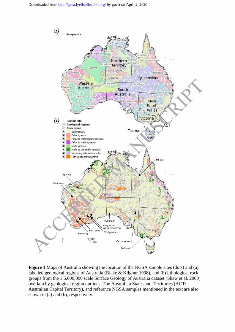
Figure 1 Maps of Australia showing the location of the NGSA sample sites (dots) and (a)
labelled geological regions of Australia (Blake & Kilgour 1998), and (b) lithological rock
groups from the 1:5,000,000 scale Surface Geology of Australia dataset (Shaw et al. 2000)
overlain by geological region outlines. The Australian States and Territories (ACT:
Australian Capital Territory), and reference NGSA samples mentioned in the text are also
shown in (a) and (b), respectively.
ACCEPTED MANUSCRIPT
by guest on April 2, 2020http://geea.lyellcollection.org/Downloaded from
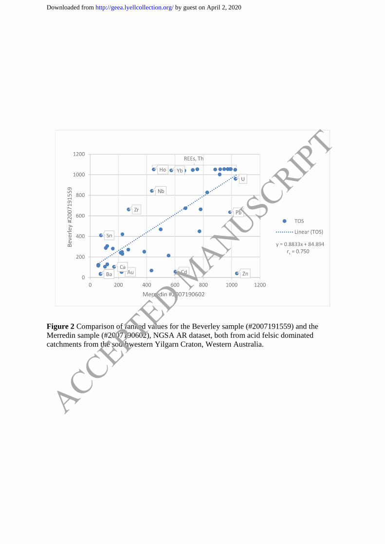
Figure 2 Comparison of ranked values for the Beverley sample (#2007191559) and the
Merredin sample (#2007190602), NGSA AR dataset, both from acid felsic dominated
catchments from the southwestern Yilgarn Craton, Western Australia.
ACCEPTED MANUSCRIPT
by guest on April 2, 2020http://geea.lyellcollection.org/Downloaded from
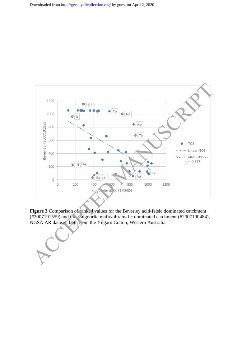
Figure 3 Comparison of ranked values for the Beverley acid-felsic dominated catchment
(#2007191559) and the Kalgoorlie mafic/ultramafic dominated catchment (#2007190484),
NGSA AR dataset, both from the Yilgarn Craton, Western Australia.
ACCEPTED MANUSCRIPT
by guest on April 2, 2020http://geea.lyellcollection.org/Downloaded from
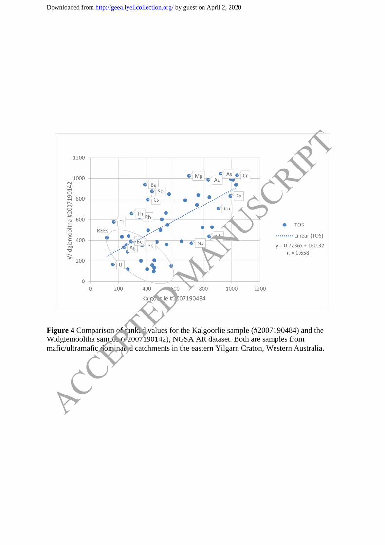
Figure 4 Comparison of ranked values for the Kalgoorlie sample (#2007190484) and the
Widgiemooltha sample (#2007190142), NGSA AR dataset. Both are samples from
mafic/ultramafic dominated catchments in the eastern Yilgarn Craton, Western Australia.
ACCEPTED MANUSCRIPT
by guest on April 2, 2020http://geea.lyellcollection.org/Downloaded from
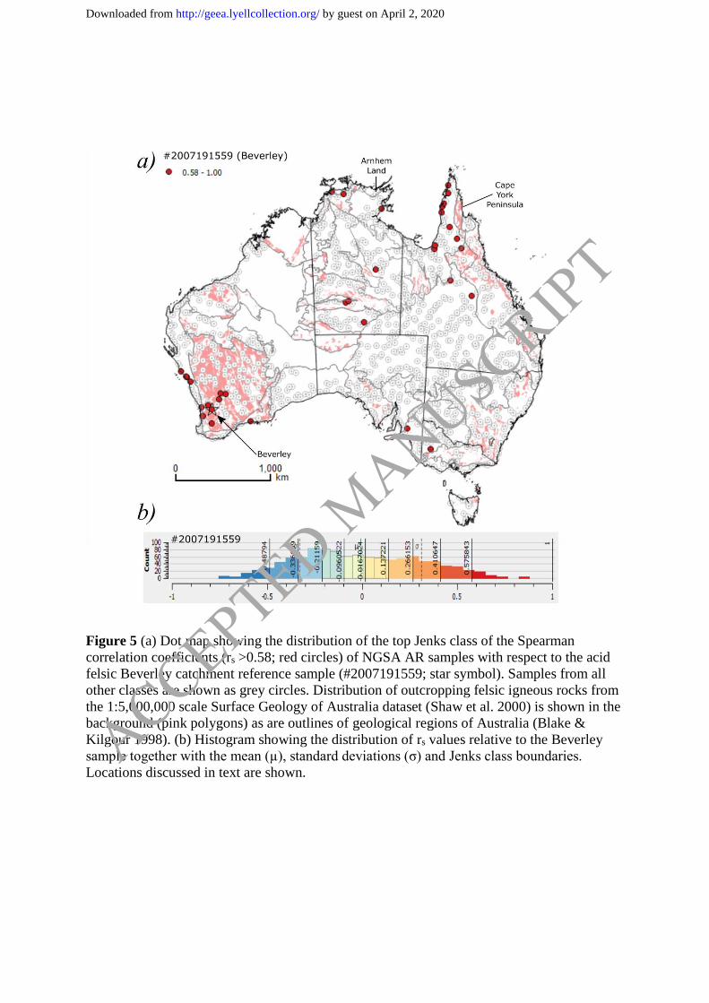
Figure 5 (a) Dot map showing the distribution of the top Jenks class of the Spearman
correlation coefficients (rs >0.58; red circles) of NGSA AR samples with respect to the acid
felsic Beverley catchment reference sample (#2007191559; star symbol). Samples from all
other classes are shown as grey circles. Distribution of outcropping felsic igneous rocks from
the 1:5,000,000 scale Surface Geology of Australia dataset (Shaw et al. 2000) is shown in the
background (pink polygons) as are outlines of geological regions of Australia (Blake &
Kilgour 1998). (b) Histogram showing the distribution of rs values relative to the Beverley
sample together with the mean (µ), standard deviations (σ) and Jenks class boundaries.
Locations discussed in text are shown. ACCEPTED M
ANUSCRIPT
by guest on April 2, 2020http://geea.lyellcollection.org/Downloaded from
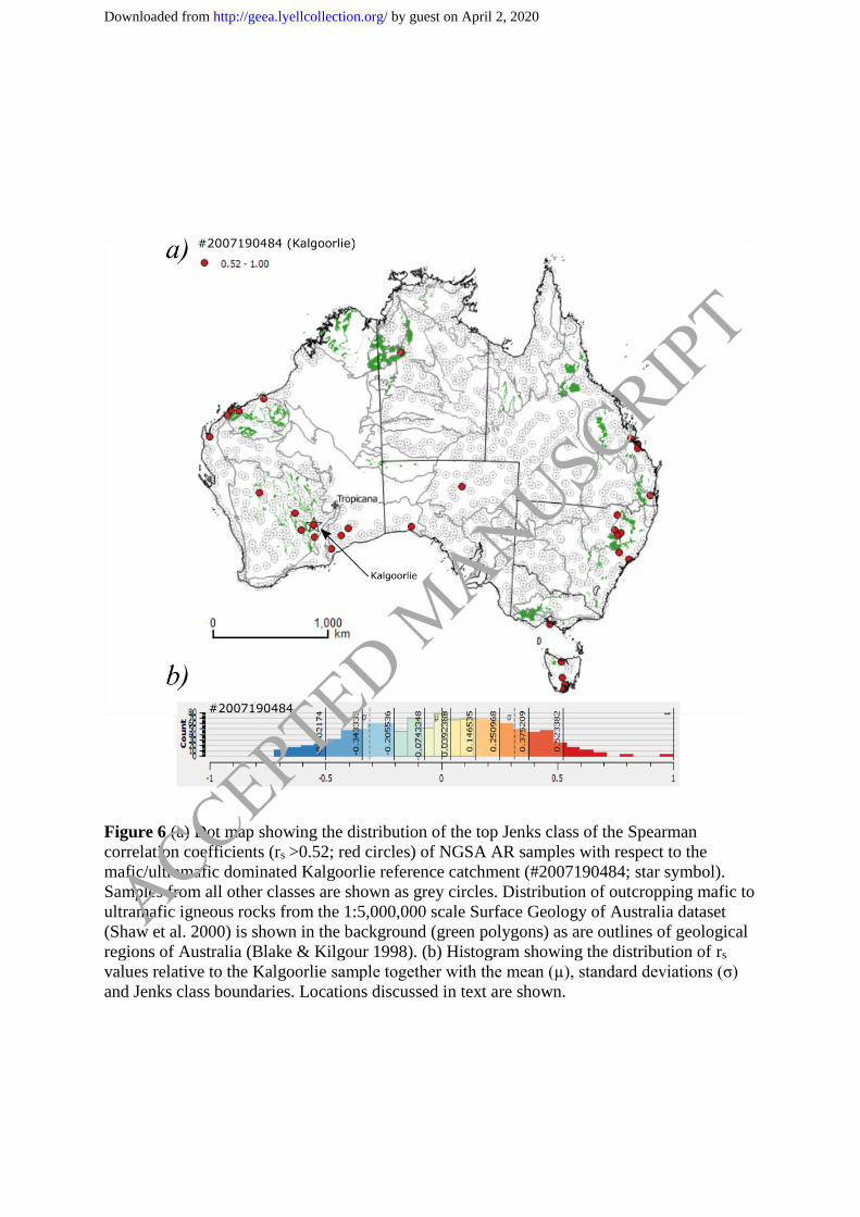
Figure 6 (a) Dot map showing the distribution of the top Jenks class of the Spearman
correlation coefficients (rs >0.52; red circles) of NGSA AR samples with respect to the
mafic/ultramafic dominated Kalgoorlie reference catchment (#2007190484; star symbol).
Samples from all other classes are shown as grey circles. Distribution of outcropping mafic to
ultramafic igneous rocks from the 1:5,000,000 scale Surface Geology of Australia dataset
(Shaw et al. 2000) is shown in the background (green polygons) as are outlines of geological
regions of Australia (Blake & Kilgour 1998). (b) Histogram showing the distribution of rs
values relative to the Kalgoorlie sample together with the mean (µ), standard deviations (σ)
and Jenks class boundaries. Locations discussed in text are shown.
ACCEPTED MANUSCRIPT
by guest on April 2, 2020http://geea.lyellcollection.org/Downloaded from
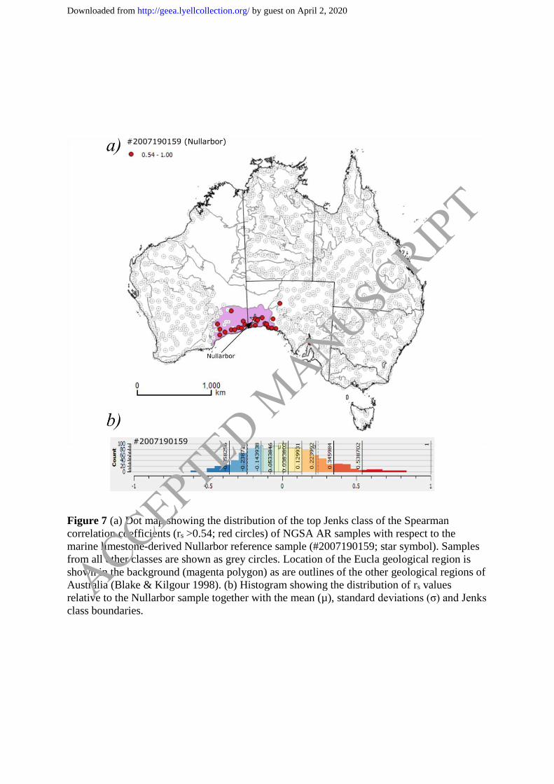
Figure 7 (a) Dot map showing the distribution of the top Jenks class of the Spearman
correlation coefficients (rs >0.54; red circles) of NGSA AR samples with respect to the
marine limestone-derived Nullarbor reference sample (#2007190159; star symbol). Samples
from all other classes are shown as grey circles. Location of the Eucla geological region is
shown in the background (magenta polygon) as are outlines of the other geological regions of
Australia (Blake & Kilgour 1998). (b) Histogram showing the distribution of rs values
relative to the Nullarbor sample together with the mean (µ), standard deviations (σ) and Jenks
class boundaries.
ACCEPTED MANUSCRIPT
by guest on April 2, 2020http://geea.lyellcollection.org/Downloaded from

Figure 8 Comparison of ranked values for the Nullarbor marine limestone-derived sample
(#2007190159) and the Gascoyne River regolith calcrete-derived sample (#2007190881),
NGSA AR dataset, from the Eucla geological region, South Australia, and Yilgarn Craton,
Western Australia, respectively.
ACCEPTED MANUSCRIPT
by guest on April 2, 2020http://geea.lyellcollection.org/Downloaded from
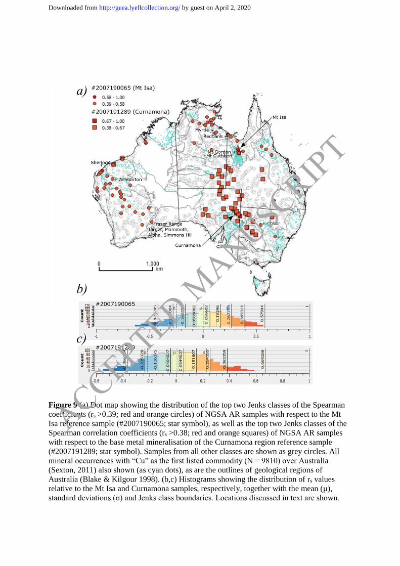
Figure 9 (a) Dot map showing the distribution of the top two Jenks classes of the Spearman
coefficients (rs >0.39; red and orange circles) of NGSA AR samples with respect to the Mt
Isa reference sample (#2007190065; star symbol), as well as the top two Jenks classes of the
Spearman correlation coefficients (rs >0.38; red and orange squares) of NGSA AR samples
with respect to the base metal mineralisation of the Curnamona region reference sample
(#2007191289; star symbol). Samples from all other classes are shown as grey circles. All
mineral occurrences with “Cu” as the first listed commodity (N = 9810) over Australia
(Sexton, 2011) also shown (as cyan dots), as are the outlines of geological regions of
Australia (Blake & Kilgour 1998). (b,c) Histograms showing the distribution of rs values
relative to the Mt Isa and Curnamona samples, respectively, together with the mean (µ),
standard deviations (σ) and Jenks class boundaries. Locations discussed in text are shown.
ACCEPTED MANUSCRIPT
by guest on April 2, 2020http://geea.lyellcollection.org/Downloaded from
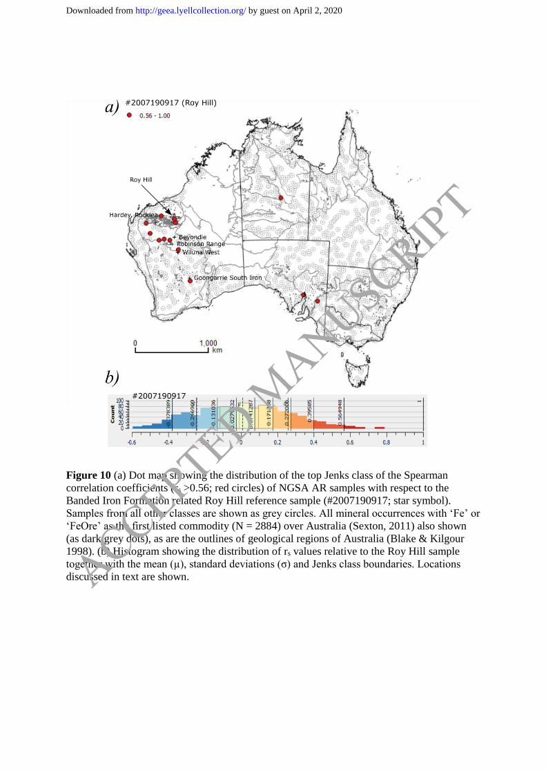
Figure 10 (a) Dot map showing the distribution of the top Jenks class of the Spearman
correlation coefficients (rs >0.56; red circles) of NGSA AR samples with respect to the
Banded Iron Formation related Roy Hill reference sample (#2007190917; star symbol).
Samples from all other classes are shown as grey circles. All mineral occurrences with ‘Fe’ or
‘FeOre’ as the first listed commodity (N = 2884) over Australia (Sexton, 2011) also shown
(as dark grey dots), as are the outlines of geological regions of Australia (Blake & Kilgour
1998). (b) Histogram showing the distribution of rs values relative to the Roy Hill sample
together with the mean (µ), standard deviations (σ) and Jenks class boundaries. Locations
discussed in text are shown. ACCEPTED MANUSCRIPT
by guest on April 2, 2020http://geea.lyellcollection.org/Downloaded from
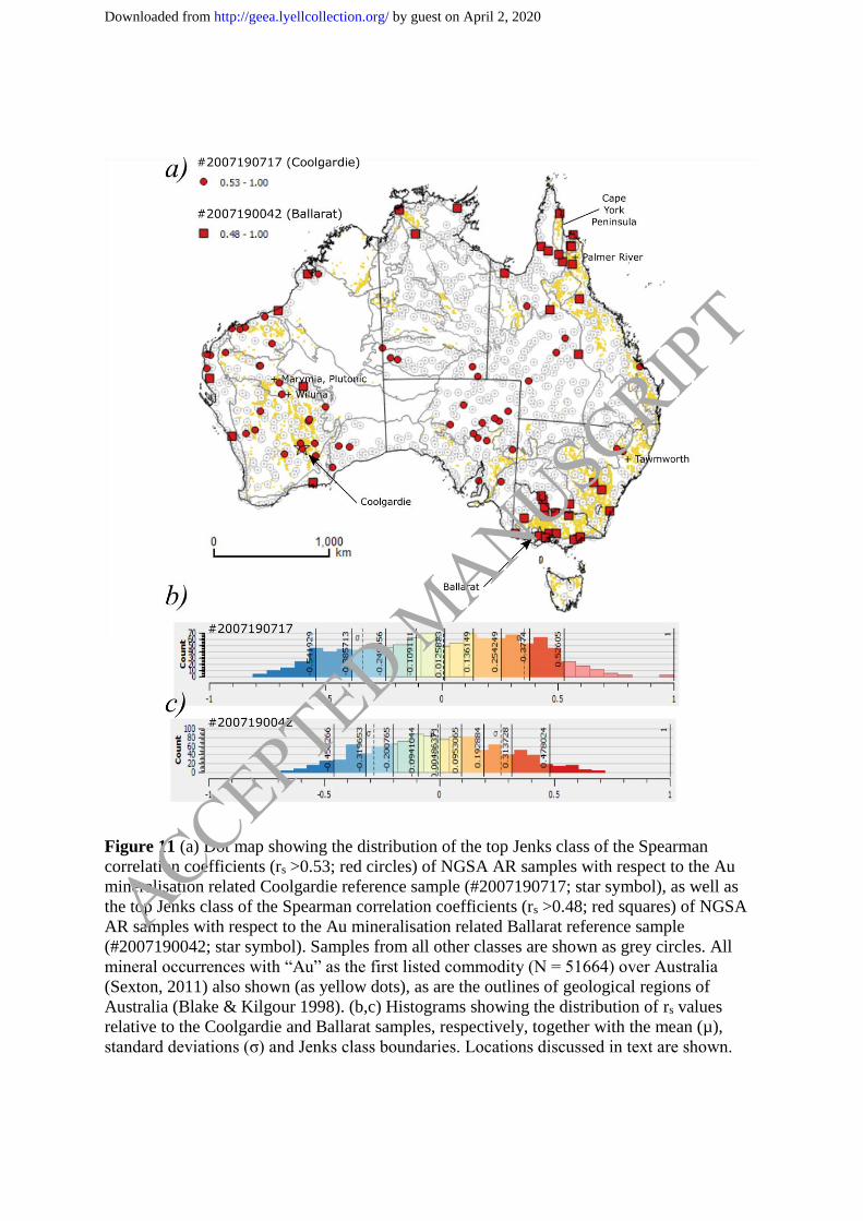
Figure 11 (a) Dot map showing the distribution of the top Jenks class of the Spearman
correlation coefficients (rs >0.53; red circles) of NGSA AR samples with respect to the Au
mineralisation related Coolgardie reference sample (#2007190717; star symbol), as well as
the top Jenks class of the Spearman correlation coefficients (rs >0.48; red squares) of NGSA
AR samples with respect to the Au mineralisation related Ballarat reference sample
(#2007190042; star symbol). Samples from all other classes are shown as grey circles. All
mineral occurrences with “Au” as the first listed commodity (N = 51664) over Australia
(Sexton, 2011) also shown (as yellow dots), as are the outlines of geological regions of
Australia (Blake & Kilgour 1998). (b,c) Histograms showing the distribution of rs values
relative to the Coolgardie and Ballarat samples, respectively, together with the mean (µ),
standard deviations (σ) and Jenks class boundaries. Locations discussed in text are shown.
ACCEPTED MANUSCRIPT
by guest on April 2, 2020http://geea.lyellcollection.org/Downloaded from
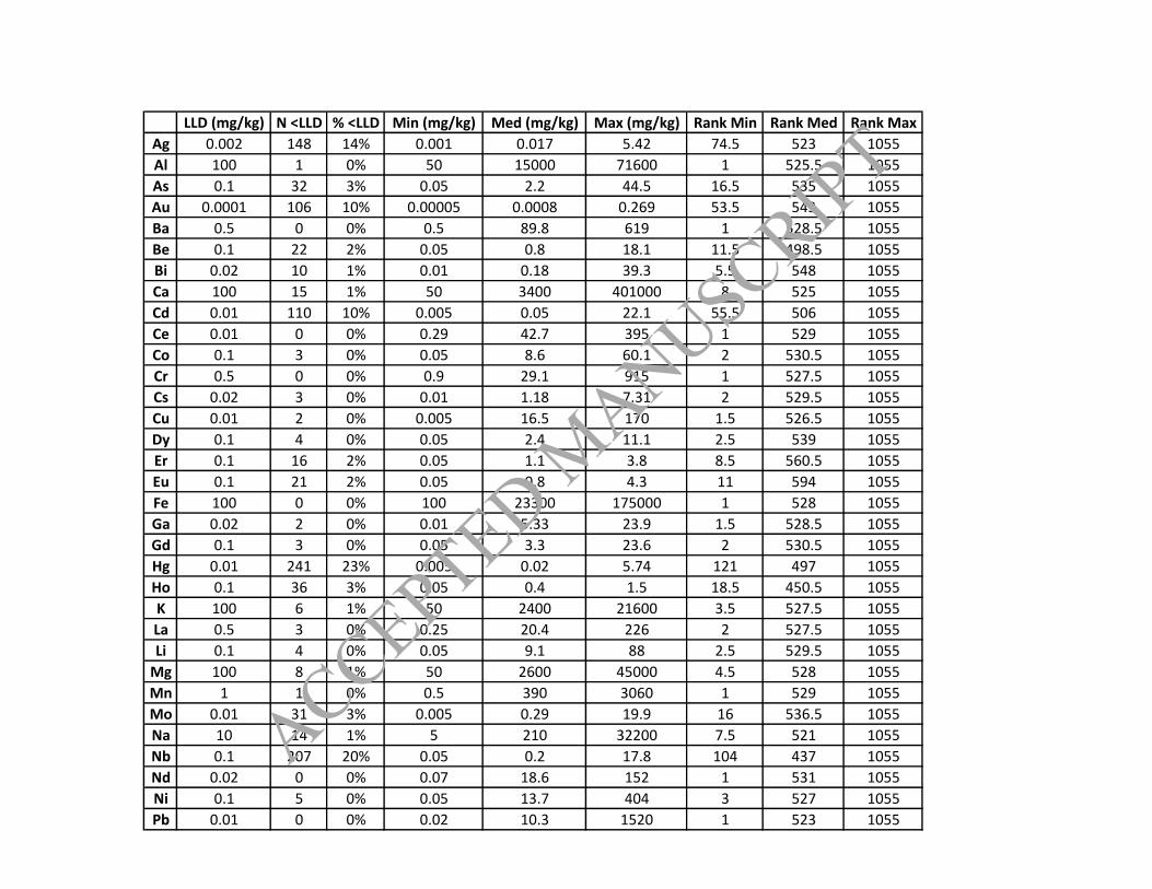
LLD (mg/kg) N <LLD % <LLD Min (mg/kg) Med (mg/kg) Max (mg/kg) Rank Min Rank Med Rank Max
Ag 0.002 148 14% 0.001 0.017 5.42 74.5 523 1055
Al 100 1 0% 50 15000 71600 1 525.5 1055
As 0.1 32 3% 0.05 2.2 44.5 16.5 535 1055
Au 0.0001 106 10% 0.00005 0.0008 0.269 53.5 543 1055
Ba 0.5 0 0% 0.5 89.8 619 1 528.5 1055
Be 0.1 22 2% 0.05 0.8 18.1 11.5 498.5 1055
Bi 0.02 10 1% 0.01 0.18 39.3 5.5 548 1055
Ca 100 15 1% 50 3400 401000 8 525 1055
Cd 0.01 110 10% 0.005 0.05 22.1 55.5 506 1055
Ce 0.01 0 0% 0.29 42.7 395 1 529 1055
Co 0.1 3 0% 0.05 8.6 60.1 2 530.5 1055
Cr 0.5 0 0% 0.9 29.1 915 1 527.5 1055
Cs 0.02 3 0% 0.01 1.18 7.31 2 529.5 1055
Cu 0.01 2 0% 0.005 16.5 170 1.5 526.5 1055
Dy 0.1 4 0% 0.05 2.4 11.1 2.5 539 1055
Er 0.1 16 2% 0.05 1.1 3.8 8.5 560.5 1055
Eu 0.1 21 2% 0.05 0.8 4.3 11 594 1055
Fe 100 0 0% 100 23300 175000 1 528 1055
Ga 0.02 2 0% 0.01 5.33 23.9 1.5 528.5 1055
Gd 0.1 3 0% 0.05 3.3 23.6 2 530.5 1055
Hg 0.01 241 23% 0.005 0.02 5.74 121 497 1055
Ho 0.1 36 3% 0.05 0.4 1.5 18.5 450.5 1055
K 100 6 1% 50 2400 21600 3.5 527.5 1055
La 0.5 3 0% 0.25 20.4 226 2 527.5 1055
Li 0.1 4 0% 0.05 9.1 88 2.5 529.5 1055
Mg 100 8 1% 50 2600 45000 4.5 528 1055
Mn 1 1 0% 0.5 390 3060 1 529 1055
Mo 0.01 31 3% 0.005 0.29 19.9 16 536.5 1055
Na 10 14 1% 5 210 32200 7.5 521 1055
Nb 0.1 207 20% 0.05 0.2 17.8 104 437 1055
Nd 0.02 0 0% 0.07 18.6 152 1 531 1055
Ni 0.1 5 0% 0.05 13.7 404 3 527 1055
Pb 0.01 0 0% 0.02 10.3 1520 1 523 1055
ACCEPTED MANUSCRIPT
by guest on April 2, 2020http://geea.lyellcollection.org/Downloaded from
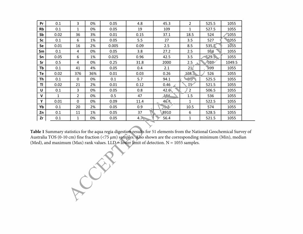
Pr 0.1 3 0% 0.05 4.8 45.3 2 525.5 1055
Rb 0.1 1 0% 0.05 19 109 1 527.5 1055
Sb 0.02 36 3% 0.01 0.15 37.1 18.5 524 1055
Sc 0.1 6 1% 0.05 5.5 27 3.5 527 1055
Se 0.01 16 2% 0.005 0.09 2.5 8.5 535.5 1055
Sm 0.1 4 0% 0.05 3.8 27.2 2.5 534 1055
Sn 0.05 6 1% 0.025 0.96 42.5 3.5 529.5 1055
Sr 0.5 4 0% 0.25 31.8 2000 2.5 528 1049.5
Tb 0.1 41 4% 0.05 0.4 2.1 21 499 1055
Te 0.02 376 36% 0.01 0.03 0.26 188.5 526 1055
Th 0.1 0 0% 0.1 5.7 94.1 2.5 525.5 1055
Tl 0.02 21 2% 0.01 0.12 0.46 11 521.5 1055
U 0.1 3 0% 0.05 0.8 42.6 2 506.5 1055
V 1 2 0% 0.5 47 184 1.5 536 1055
Y 0.01 0 0% 0.09 11.4 46.4 1 522.5 1055
Yb 0.1 20 2% 0.05 0.9 3.2 10.5 574 1055
Zn 0.1 11 1% 0.05 37 8910 6 528.5 1055
Zr 0.1 1 0% 0.05 4.7 56.4 1 521.5 1055
ACCEPTED MANUSC
RIPT
Table 1 Summary statistics for the aqua regia digestion results for 51 elements from the National Geochemical Survey of Australia TOS (0-10 cm) fine fraction (<75 µm) samples. Also shown are the corresponding minimum (Min), median (Med), and maximum (Max) rank values. LLD = lower limit of detection. N = 1055 samples.
by guest on April 2, 2020http://geea.lyellcollection.org/Downloaded from
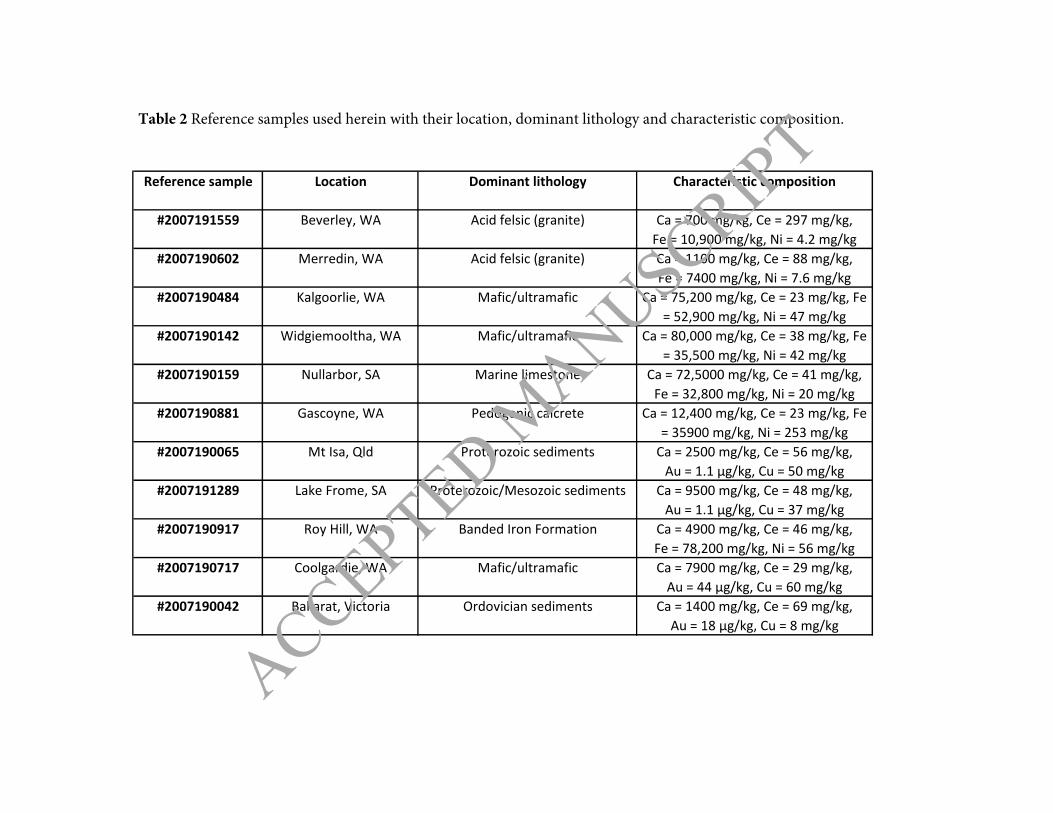
Reference sample Location Dominant lithology Characteristic composition
#2007191559 Beverley, WA Acid felsic (granite) Ca = 700 mg/kg, Ce = 297 mg/kg,
Fe = 10,900 mg/kg, Ni = 4.2 mg/kg
#2007190602 Merredin, WA Acid felsic (granite) Ca = 1100 mg/kg, Ce = 88 mg/kg,
Fe = 7400 mg/kg, Ni = 7.6 mg/kg
#2007190484 Kalgoorlie, WA Mafic/ultramafic Ca = 75,200 mg/kg, Ce = 23 mg/kg, Fe
= 52,900 mg/kg, Ni = 47 mg/kg
#2007190142 Widgiemooltha, WA Mafic/ultramafic Ca = 80,000 mg/kg, Ce = 38 mg/kg, Fe
= 35,500 mg/kg, Ni = 42 mg/kg
#2007190159 Nullarbor, SA Marine limestone Ca = 72,5000 mg/kg, Ce = 41 mg/kg,
Fe = 32,800 mg/kg, Ni = 20 mg/kg
#2007190881 Gascoyne, WA Pedogenic calcrete Ca = 12,400 mg/kg, Ce = 23 mg/kg, Fe
= 35900 mg/kg, Ni = 253 mg/kg
#2007190065 Mt Isa, Qld Proterozoic sediments Ca = 2500 mg/kg, Ce = 56 mg/kg,
Au = 1.1 µg/kg, Cu = 50 mg/kg
#2007191289 Lake Frome, SA Proterozoic/Mesozoic sediments Ca = 9500 mg/kg, Ce = 48 mg/kg,
Au = 1.1 µg/kg, Cu = 37 mg/kg
#2007190917 Roy Hill, WA Banded Iron Formation Ca = 4900 mg/kg, Ce = 46 mg/kg,
Fe = 78,200 mg/kg, Ni = 56 mg/kg
#2007190717 Coolgardie, WA Mafic/ultramafic Ca = 7900 mg/kg, Ce = 29 mg/kg,
Au = 44 µg/kg, Cu = 60 mg/kg
#2007190042 Ballarat, Victoria Ordovician sediments Ca = 1400 mg/kg, Ce = 69 mg/kg,
Au = 18 µg/kg, Cu = 8 mg/kg
Table 2 Reference samples used herein with their location, dominant lithology and characteristic composition.
ACCEPTED MANUSCRIPT
by guest on April 2, 2020http://geea.lyellcollection.org/Downloaded from
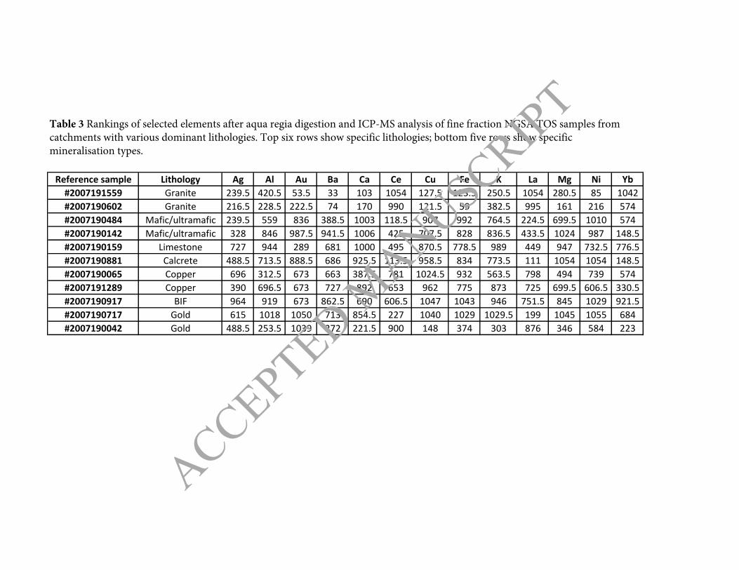
Reference sample Lithology Ag Al Au Ba Ca Ce Cu Fe K La Mg Ni Yb
#2007191559 Granite 239.5 420.5 53.5 33 103 1054 127.5 123.5 250.5 1054 280.5 85 1042
#2007190602 Granite 216.5 228.5 222.5 74 170 990 121.5 59 382.5 995 161 216 574
#2007190484 Mafic/ultramafic 239.5 559 836 388.5 1003 118.5 907 992 764.5 224.5 699.5 1010 574
#2007190142 Mafic/ultramafic 328 846 987.5 941.5 1006 425 707.5 828 836.5 433.5 1024 987 148.5
#2007190159 Limestone 727 944 289 681 1000 495 870.5 778.5 989 449 947 732.5 776.5
#2007190881 Calcrete 488.5 713.5 888.5 686 925.5 113.5 958.5 834 773.5 111 1054 1054 148.5
#2007190065 Copper 696 312.5 673 663 387.5 781 1024.5 932 563.5 798 494 739 574
#2007191289 Copper 390 696.5 673 727 892 653 962 775 873 725 699.5 606.5 330.5
#2007190917 BIF 964 919 673 862.5 690 606.5 1047 1043 946 751.5 845 1029 921.5
#2007190717 Gold 615 1018 1050 713 854.5 227 1040 1029 1029.5 199 1045 1055 684
#2007190042 Gold 488.5 253.5 1039 272 221.5 900 148 374 303 876 346 584 223
Table 3 Rankings of selected elements after aqua regia digestion and ICP-MS analysis of fine fraction NGSA TOS samples from catchments with various dominant lithologies. Top six rows show specific lithologies; bottom five rows show specific mineralisation types.
ACCEPTED MANUSCRIPT
by guest on April 2, 2020http://geea.lyellcollection.org/Downloaded from
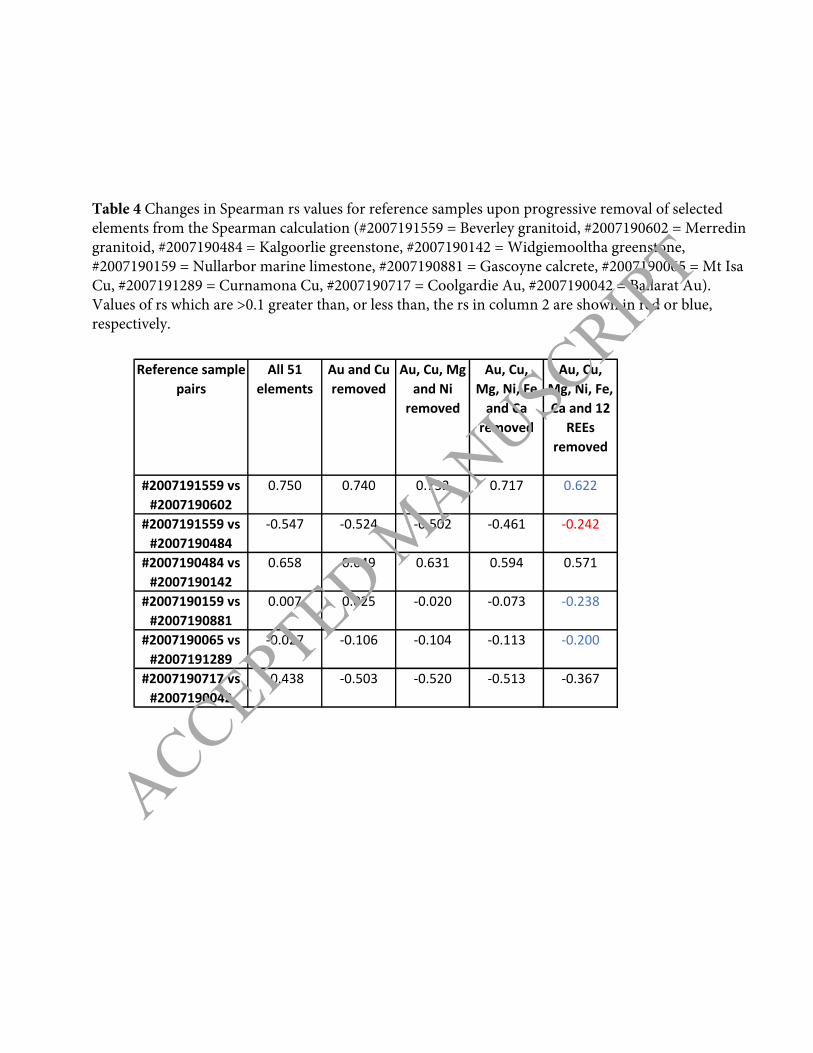
Reference sample
pairs
All 51
elements
Au and Cu
removed
Au, Cu, Mg
and Ni
removed
Au, Cu,
Mg, Ni, Fe
and Ca
removed
Au, Cu,
Mg, Ni, Fe,
Ca and 12
REEs
removed
#2007191559 vs
#2007190602
0.750 0.740 0.732 0.717 0.622
#2007191559 vs
#2007190484
-0.547 -0.524 -0.502 -0.461 -0.242
#2007190484 vs
#2007190142
0.658 0.649 0.631 0.594 0.571
#2007190159 vs
#2007190881
0.007 0.025 -0.020 -0.073 -0.238
#2007190065 vs
#2007191289
-0.027 -0.106 -0.104 -0.113 -0.200
#2007190717 vs
#2007190042
-0.438 -0.503 -0.520 -0.513 -0.367
Table 4 Changes in Spearman rs values for reference samples upon progressive removal of selected elements from the Spearman calculation (#2007191559 = Beverley granitoid, #2007190602 = Merredin granitoid, #2007190484 = Kalgoorlie greenstone, #2007190142 = Widgiemooltha greenstone, #2007190159 = Nullarbor marine limestone, #2007190881 = Gascoyne calcrete, #2007190065 = Mt Isa Cu, #2007191289 = Curnamona Cu, #2007190717 = Coolgardie Au, #2007190042 = Ballarat Au). Values of rs which are >0.1 greater than, or less than, the rs in column 2 are shown in red or blue, respectively.
ACCEPTED MANUSCRIPT
by guest on April 2, 2020http://geea.lyellcollection.org/Downloaded from


