1
Globalization and Poverty in Senegal: A Worst Case Scenario?
Miet Maertensa, Liesbeth Colenb and Johan F.M. Swinnenb
a Department of Earth and Environmental Science, Division Agricultural and Food Economics, K.U.Leuven
b LICOS Centre for Institutions and Economic Performance & Department of Economics, K.U.Leuven, www.econ.kuleuven.be/licos
Contact: [email protected]; [email protected]
Contributed Paper prepared for presentation at the International Association of Agricultural Economists Conference, Beijing, China, August 16-22, 2009
Copyright 2009 by Miet Maertens, Liesbeth Colen and Johan F.M. Swinnen. All rights reserved. Readers may make verbatim copies of this document for non-commercial purposes by any means, provided that this copyright notice appears on all such copies.
2
Globalization and Poverty in Senegal:
A Worst Case Scenario?
Miet Maertens, Liesbeth Colen and Johan F.M. Swinnen
LICOS Centre for Institutions and Economic Performance & Department of Economics
K.U.Leuven
www.econ.kuleuven.be/licos
Abstract
There is no consensus about how globalization –trade and foreign investments –
affects poverty reduction. Using household survey data, this study contributes to the
empirical literature on globalization and poverty by analyzing the household-level
implications of increased foreign investments and trade in the horticulture sector in
Senegal. In many aspects this represents what many would consider a “worst-case
scenario”. Stringent rich country standards are imposed on exports and the supply
chain is controlled by a single multinational company with extreme levels of supply
base consolidation, full vertical integration and complete exclusion of smallholder
suppliers. We analyze and quantify income and poverty effects under these “worst-
case conditions” and find significant positive welfare impacts through employment
creation and labor market participation.
Keywords: trade, FDI, poverty, vertical coordination, modern supply chains
JEL: F2, J43, O12, Q12, Q17
Corresponding author: [email protected]
3
Globalization and Poverty in Senegal:
A Worst Case Scenario?
1. Introduction
There is no consensus about how globalization – trade and foreign investments
– affects poverty reduction. Participation in international trade has been advocated as
a major engine of growth in poor countries1 (Dollar and Kraay, 2002; Frankel and
Romer, 1999; Irwin and Tervio, 2002). In addition, developing countries are said to
benefit considerably from the inflow of foreign direct investment (FDI) through direct
growth effects and a variety of growth spillover effects2 (Blalock and Gertler, 2008;
Borenzstein et al., 1998; Choe, 2003; Hansen and Rand, 2006; Xu, 2000). However,
there is much less consensus about how foreign trade and investment specifically
affect the poor in these countries. Some authors point to evidence of poverty-
alleviating effects of trade (Ben-David, 1996; Bhagwati and Srinivasan, 2002; Dollar
and Kraay, 2004;) while others contradict this assertion (Fosu and Mold, 2008;
Lundberg and Squire, 2003; Ravallion, 2001 & 2006). Likewise, some see FDI as an
effective tool in the fight against poverty (Klein et al., 2001; UNCTAD, 2005) while
others argue this is highly overestimated (Nunnenkamp, 2004). Some studies present
evidence of a negative link between FDI inflows and inequality in developing
countries (Feenstra and Hanson, 1997; Jensen and Rosas, 2007) while others have
demonstrated the absence of such a link (Lindert and Williamson, 2001; Milanovic,
2002) or even the opposite (Agénor, 2004; Choi, 2006; Tsai, 1995). In summary, there
is no general conclusion about how the integration of developing countries in global 1 See Rodriguez and Rodrik (2000) for a critique on this conclusion and Winters et al. (2004) for a survey of the arguments. 2 See Kosack and Tobin (2006) for a critique on this conclusion. See Klein et al. (2001) and Colen et al. (2008) for a review of the direct and indirect growth effects of FDI and Hansen and Rand (2006) for a discussion on the factors conditioning the magnitude of the growth effect of FDI in poor countries.
4
markets affects poverty and income inequality in these countries (Winters et al., 2004;
Cooper, 2002). This lack of consensus has induced a call for more convincing
empirical evidence on the link between globalization and poverty dynamics at the
household level (Winters et al., 2004, pp.107) and for evidence from country case-
studies – rather than cross-country regressions (Srinvasan and Bhagwati, 2001).
The aim of this study is therefore to contribute to the empirical literature on
globalization and poverty by using household data to study the effects of what many
would ex ante consider a “worst case scenario”, i.e. FDI and trade growth in the
tomato export sector in Senegal. This case of globalization has several characteristics
which have been argued to be detrimental to the rural poor in developing countries:
(a) Senegal is a very poor country with many institutional problems and market
imperfections; (b) the fresh fruit and vegetable (FFV) sector has faced rapidly
tightening and currently very stringent standards on products and production
processes; (c) the export tomato chain is characterized by extreme consolidation, as a
single company controls all the production, processing, and trade; (d) the monopoly
exporting company is a foreign multinational company; (e) the various levels in the
supply chain are fully vertically integrated; and (f) smallholders are completely
excluded as all tomatoes for export are produced on large scale farms owned by the
exporting company.
The agri-food sector is of particular relevance to situate the impact of
economic globalization on poverty. On the one hand, stimulating agri-food exports
and attracting FDI in the agri-food sector have been promoted as pro-poor growth
strategies because of the direct link the sector has with the rural economy – where
poverty rates are often much higher than in urban areas – and because of the intensive
use of unskilled labor in the sector (Aksoy and Beghin, 2005; Anderson and Martin,
5
2005; Carter et al., 1996; World Bank, 2008). On the other hand, increased
globalization of the agri-food sector has been argued to be detrimental for global
poverty reduction as the poorest countries and the poorest farmers are increasingly
excluded and marginalized. Rapidly growing foreign investments in food processing
and retailing sectors3 and the recent proliferation of stringent food standards –
resulting from these investments as well as from increased attention to food quality
and safety in high-income countries and markets – are causing shifts in global food
supply chains with an increased dominance of large multinational food companies,
consolidation of the supply base and increased vertical coordination in the chains
(Farina and Reardon, 2000; Reardon et al., 1999; Swinnen, 2005 and 2007; Swinnen
and Maertens, 2007; Weatherspoon and Reardon, 2003). Major concerns of these
recent developments are (a) that standards act as new non-tariff barriers diminishing
the export opportunities of the poorest countries for whom compliance costs are
inhibitingly high4; (b) that poor farmers are exploited in vertically coordinated food
supply chains because of reduced bargaining power vis-à-vis large multinational food
companies; and (c) that poor suppliers are excluded from high-standards global food
supply chains because of their inability to comply with high standards5.
These arguments are subject to debate. First, some studies have pointed to
cases where increasing food standards are applied to the competitive advantage of
developing countries, resulting in upgrading of the food sector and enhanced market
access (Jaffee and Henson, 2004 & 2005; Henson and Jaffee, 2008; Maertens and
3 One of the most publicized aspects of these investments is the so-called supermarket revolution, discussed by Reardon and Berdegué (2002); Reardon et al. (2003), and Weatherspoon and Reardon (2003). 4 See Jaffee and Henson (2005); Garcia Martinez and Poole, 2004; Unnevehr (2000); and Wilson and Abiola (2003) for a more detailed discussion. 5 Gibbon (2003), Key and Runsten (1999), Maertens and Swinnen (2007); Swinnen (2007), and World Bank (2005) discuss the grounds for the marginalisation and the exclusion of small and resource-poor farmers.

6
Swinnen, 2007). Second, rather than being exploited, small farmers can gain
importantly in vertical coordination schemes with the agro-industry through
enhanced access to inputs, reduced production and marketing risks, improved
technology and productivity, and ultimately higher incomes – which has been
empirically demonstrated by various authors (Dries and Swinnen, 2004; Gulati et al.,
2007; Minten et al., 2008; Swinnen, 2005). Third, the extent of smallholder exclusion
in globalized food supply chains is a controversial issue. Some empirical studies find
that the reorganization of global food supply chains have led to a shift from
smallholder production to agro-industrial production, thereby excluding smallholders
from profitable trading opportunities and resulting in negative welfare effects
(Danielou and Ravry, 2005; Farina and Reardon, 2000; Key and Runsten, 1999;
Reardon et al., 1999; Reardon et al., 2003; Weatherspoon and Reardon, 2003). Others
have come to more moderate conclusions on the extent of smallholder exclusion
(Jaffee, 2003 ; Kherralah, 2000; Minot and Ngigi, 2004; Swinnen, 2007).
However, surprisingly little research has focused on the overall poverty effects
of globalization in agri-food sectors of developing countries. Most of the above
mentioned studies focus only on production linkages when analyzing the effects of
increased agri-food trade and investments. Yet, the poor may benefit through labor
markets as well. The intensive use of unskilled labor in agri-food sectors has been put
forward as a main potential source of poverty reduction (e.g Carter et al., 1996). A
couple of recent studies have indeed pointed to the welfare gains from employment
opportunities in the emerging agro-industry (Barron and Rello, 2000; Maertens and
Swinnen, 2008; McCulloh and Ota, 2002). Apart from the latter studies, surprisingly
little attention has been paid to labor markets in the discussion on the link between
7
globalization in the agri-food sector and poverty – and none has analyzed an extreme
case as is the very subject of our research.
We use unique household level survey data combined with complementary
data from company and village interviews to assess the implications of production and
trade in the tomato sector in Senegal for income and poverty dynamics. Our study
yields several important findings. First, we find that tomato exports from Senegal to
the EU have increased sharply over the past decade, despite increasing standards in
the EU. Second, despite the extreme consolidation and vertical integration in the
supply chain and the exclusion of smallholder farms from export tomato production,
tomato exports contribute importantly to poor household incomes and poverty
reduction in the tomato producing regions through employment effects. Third, we do
not find evidence that asset-poor households or unskilled individuals are
disadvantaged in accessing employment in the tomato export chain.
The structure of the paper is as follows. In the next section we discuss the
developments in the tomato export supply chain in Senegal – including the
importance of standards. In section three we present details on the survey data that are
used to analyze the welfare implications of export tomato development. In section
four we discuss the implications for rural employment, income mobility and poverty
based on descriptive statistics. In section five we present an econometric model to
analyze the income effects and discuss the derived results. We draw some conclusions
in a final section.
2. The Tomato Export Supply Chain
Horticulture Export Growth
8
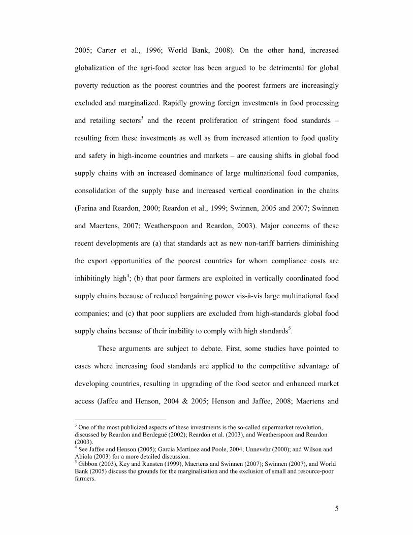
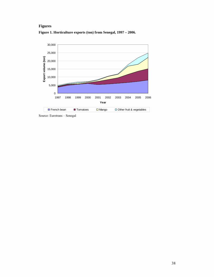
Exports of fresh fruits and vegetables (FFV) from Senegal have increased
tremendously in the past 10 years: from 4,800 ton in 1998 to almost 25,000 ton in
2007 (Figure 1). FFV exports also became more diversified. In 1997 more than 75%
of FFV exports consisted of one crop (French beans). Since the early 2000s also the
export of tomatoes and mango has grown. The export volume of tomatoes – mainly
cherry tomatoes – has increased from less than 1,000 ton in the year 2000 to almost
7,000 ton in 2007, accounting for 28% of total FFV exports.
The large majority of exported fruits and vegetables are destined for the EU-
market, mainly France, Belgium, Luxembourg and the Netherlands. Some minor
volumes of mango and other fruits are exported to neighboring countries such as Mali,
Mauretania, and Cape Verde.
Foreign Direct Investment
Foreign direct investment has played a major role in the boom of cherry
tomato exports. The initial export of tomatoes in the 2000/2001 season was realized
through two Senegalese companies specialized in the export of French beans.
However, in 2001 a foreign company – Grands Domaines du Senegal (GDS), a
subsidiary of a French holding with food production and distribution affiliates in a
number of countries in Europe, Africa and Latin-America – entered the FFV export
market in Senegal. After an initial start-up period, this company began to export
significant volumes of cherry tomatoes to the EU from 2003 onwards. After the
entrance of the FDI company, the market structure significantly changed. The market
share of GDS increased from 43% of tomato exports during the 2004/2005 season to
99% during the last completed export season (2006/2007).
9
GDS is exporting cherry tomatoes from the area of the Senegal River Delta in
the region of Saint-Louis. The company chose this area close to the Senegal River to
avoid problems of land and water shortage that is plaguing horticulture production in
other regions.
Public and Private Standards
It is remarkable that Senegal experienced accelerated export growth to the EU
in the horticulture sector during a period when food quality and safety standards
increased substantially, especially for fresh food products such as fruits and
vegetables. First, FFV exports to the EU have to satisfy a series of stringent public
quality and safety standards. EU legislation imposes (1) marketing standards for fresh
fruits and vegetables; (2) labeling requirements for foodstuffs; and (3) health control
of foodstuffs. The latter includes general conditions concerning contaminants in food,
general hygiene rules based on HACCP control mechanisms, and traceability
requirements – laid down in the General Food Law of 2002.
Second, private standard play an increasingly important role in trade of fresh
fruit and vegetables. Private retailers, traders and food processors have engaged in
initiatives to establish private standards (often more stringent than public
requirements) and adapt food quality and safety standards in certification protocols.
Although private standards are legally not mandatory they have become de facto
mandatory as a large share of buyers in EU markets is requiring compliance with such
standards, for example the EurepGAP standards.
In response to these increasing food standards, GDS has obtained EurepGAP
certification for the production and export of cherry tomatoes since 2003. In fact, the
multinational holding to which GDS belongs, specifically aims at high-standards
10
production and seeks compliance with a large variety of private standards including
food quality standards, food safety standards, ethical and environmental standards.
For all its plantations the holding is certified by several private certification schemes
including the International Organization for Standardization (ISO), British Retail
Consortium (BRC), European Retail Produce Working Group (EurepGAP), Ethical
Trade Initiative (ETI), Tesco Nature Choice, etc.
Consolidation and Vertical Integration
Many studies have documented important structural transformations in the
supply chains of fresh produce for export to high-standards markets (Swinnen, 2007).
High-standards agri-food supply chains have become increasingly consolidated, with
fewer and larger firms, while the level of vertical coordination in the chains is
increasing. In some cases – for example in the Malagasy FFV sector (Minten et al.,
2006) – increased standards have led to institutional innovations, such as extensive
monitoring and complex contracting, to source from small farmers. In other cases this
is associated with a shift from smallholder contract-based production to large-scale
integrated estate production, documented e.g. by Jaffee (2003) for Kenyan vegetable
exports, Minot and Ngigi (2004) for FFV exports from Cote d’Ivoire, Maertens and
Swinnen (2008) for French bean exports from Senegal, and Danielou and Ravry
(2005) for pineapple exports in Ghana. Increasing quality and safety requirements are
usually mentioned as the main driving factor behind the observed supply chains
restructuring.
The case of cherry tomato exports in Senegal represents an extreme case of
these developments of consolidation and increased vertical coordination in food
supply chains. Ninety-nine percent of the tomato exports from Senegal are handled by
11
one multinational company. Moreover, at several nodes in the chain, vertical
coordination takes the extreme form of complete ownership integration. Downstream
trading, transport and distribution activities are completely integrated within the
multinational holding with own transport and distribution subsidiaries. The maritime
company of the group has eight specialist vessels and organizes overseas transport
between 4 ports in West-Africa – including Dakar – and several ports in the EU,
mostly France, Belgium and the UK, from where further distribution in Europe is
handled by several trading affiliates of the group.
Also upstream the cherry tomato supply chain is completely vertically
integrated. For the supply of primary produce, the company relies completely on their
own integrated agro-industrial production. In the Senegal River Delta, GDS has
established a conditioning station for handling and processing fresh vegetables and
two production sites, including 40 ha of greenhouse production and 150 ha of open
field production. The company invested in irrigation infrastructure and high-
technology production techniques, including mechanized and computerized irrigation,
fertilization and phytosanitary care in a drip-to-drip system. These technologies –
along with the required inputs such as improved seeds, fertilizers and phytosanitary
products – are imported from the EU.
Hence, the tomato export supply chain excludes smallholder producers
completely as production is realized exclusively on the large-scale plantations of the
exporting company. It is important to note however, that this integrated agro-
industrial farming was not developed by buying or renting land from small farms, but
by investing in previously uncultivated land allocated to them by the government. An
additional 400 ha of land in the region of the Senegal River Delta has been assigned to
GDS by the government to expand its production and export activities in the future.
12
During interviews with GDS in September 2005 and March 2006, two main
reasons were mentioned for this strategy of complete vertical integration. First, this
strategy is in line with the policy of the French holding to which GDS belongs and
which owns similar vertically integrated production and exporting facilities in other
developing countries (e.g. in Mauretania and Côte d’Ivoire). Second, high EU
requirements on quality and food safety – such as traceability, maximum residue
levels, etc. - combined with the general low capacity and limited access to resources
(especially irrigation-water) of the local smallholder farmers induced the company to
integrate the production stage of the chain and set up their own agro-industrial farms.
A Worst-case Scenario of Supply Chain Development?
In the development literature consolidation and increased vertical integration
in agri-food supply chains – often produced under pressure of increasing food
standards – are usually considered to be particularly detrimental from a development
perspective. The main argument is that local small – often poor – farmers are
increasingly excluded from high-standards supply chains if these chains move
towards more vertical coordination and that hence the benefits of high-standards trade
are concentrated in the hands of a few large companies (Gibbon, 2003; Farina and
Reardon, 2000; Kherralah, 2000; Reardon et al., 1999). Moreover, consolidation and
FDI in the agri-food industry is expected to lead to unequal bargaining power for
farmers vis-à-vis large (multinational) companies, resulting in rent extracting by these
companies (Gibbon, 2003; Warning and Key, 2002). In addition, vertical integration
is argued to limit the possibilities of additional beneficial development effects through
spillover effects in down- and upstream activities. So, in many respects the sector
13
which we study represents what many would consider a “worst-case-scenario” of
supply chain development.
3. Data and Research Area
To study the welfare implications of the growth of the tomato export chain in
Senegal, we organized extensive primary data collection. First, in September 2005
and again in March 2006, we conducted interviews with the company GDS that
started to export tomatoes from Senegal in 2003 and accounted for 99% of tomato
exports in 2006/2007. These were mainly qualitative interviews on a diversity of
topics related to the production and exporting activities of the company. Second, we
collected qualitative information in three villages (Ndioudoune, Maka and Mbarigo)
near the production- sites of the firm through informal group interviews with the
village chief, the council of village elderly, and representatives of village
organizations. This information was mainly used to fine-tune further quantitative data
collection. Finally, in the period February-April 2006 we organized a large and
comprehensive household survey in the area surrounding the tomato exporting
company and complemented this with a village census in all sampled villages.
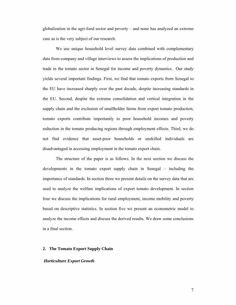
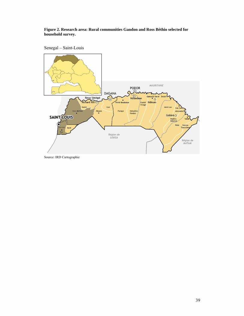
The surveys covered 299 households in 18 villages in 2 rural communities –
Gandon, the community where the company is based, and Ross Bethio, an adjacent
community. Both communities are located in the region Saint-Louis, in the north of
the country along the Senegal River (Figure 2). Villages in the sample were selected
randomly while households within the villages were stratified according to whether or
not one or several members of the households are employed in the tomato export
industry. The household selection resulted in an oversampling of households having
members employed in the tomato export industry. To draw correct inferences, this
14
oversampling is corrected for using sampling weights that are calculated with
information from a village census in all sampled villages.
The survey data – including recall data – provide details on household
demographic characteristics, land and non-land asset holdings, agricultural
production, off-farm employment, non-labor income, credit, and savings; and allow
the calculation of household net income from farm and off-farm sources. For each
household we collected detailed and recall information on the employment of
household members in the tomato export agro-industry.
4. Rural Employment, Income and Poverty – Descriptive Analysis
We want to investigate the impact of the growth in tomato exports – taking
into account the specific supply chain structure – on the welfare of the local
population. Since the chain is completely integrated and smallholder producers are not
included in the chain, the main effects come from employment creation. In this
section we first describe the participation of local households in this employment and
then present some descriptive statistics on how employment is correlated with
household income and poverty in the region. In section 5 we will use more
sophisticated statistical methods to assess the employment effects.
Employment in the Tomato Export Agro- industry
The increased export of tomatoes by GDS was accompanied by a large
increase in employment in this sector. Although parts of the production process is
mechanized and high-technology techniques are used, tomato production and
handling remains a labor-intensive business. While irrigation, fertilization and
phytosanitary care is completely mechanized and computerized with a drip-to-drip
15
system, the harvesting of tomatoes is done manually and requires substantive amounts
of labor. Also processing and handling of the tomatoes is labor intensive as packing
and labeling is done manually – while sorting is mechanized.
The growth of tomato exports has created employment opportunities in the
vast rural area of the Senegal River Delta. In 2006 GDS employed more than 3000
workers – on the fields as well as in the processing unit. About 80% of those workers
are temporary seasonal workers or day laborers. The large majority of workers are
recruited from nearby villages. The rest of the employees are seasonal migrants from
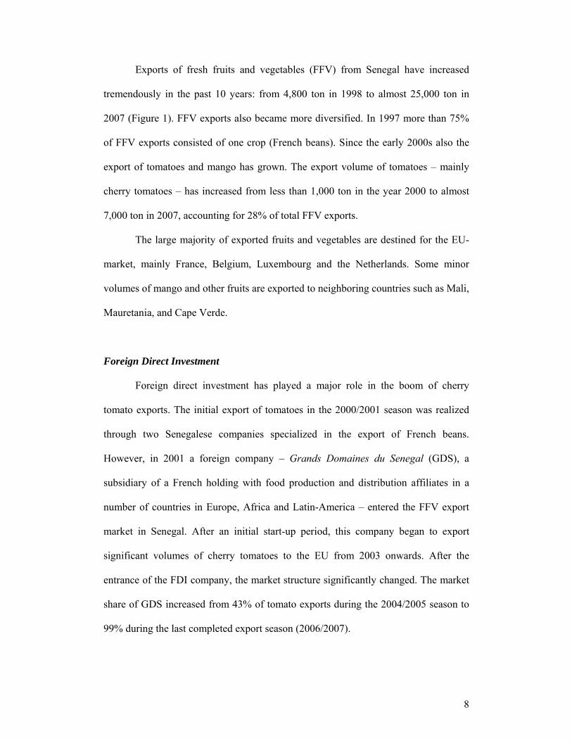
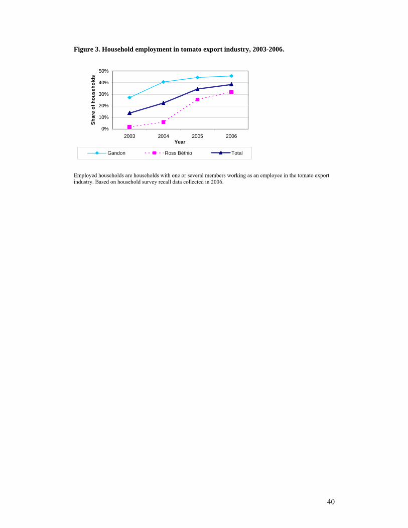
more distant locations. In our sampled villages more than one third of households
have one or more members working as employee in the tomato export industry. This
share increased from 14% in 2003 to 39% in early 2006 (Figure 3). The share is
highest – almost 50% of households – in the community Gandon which includes
villages in the immediate surroundings of the production sites and processing unit of
GDS. However, also in the adjacent community – Ross Béthio – with more distant
villages, the share of households employed by GDS is about 30%. The largest
increase in employment in this community was in 2005 when recruitment from
villages in Gandon stagnated.
The impact of tomato export growth and the associated employment on rural
income mobility, income equality and poverty reduction depends on which
households are selected into this employment and on how much they benefit. Such
employment growth could exacerbate rural income inequality if entry-constraints –
e.g. the need for a minimal level of education or certain assets – exist that limit the
off-farm employment opportunities for the poorest households. Such increase of
inequality has been observed by Dercon (1998) and Barrett et al. (2001) in studies on
rural off-farm employment in Sub-Saharan Africa. However, we find that in the case
16
of employment growth in the tomato export industry in Senegal, there appears to be
no increase in inequality, to the contrary.
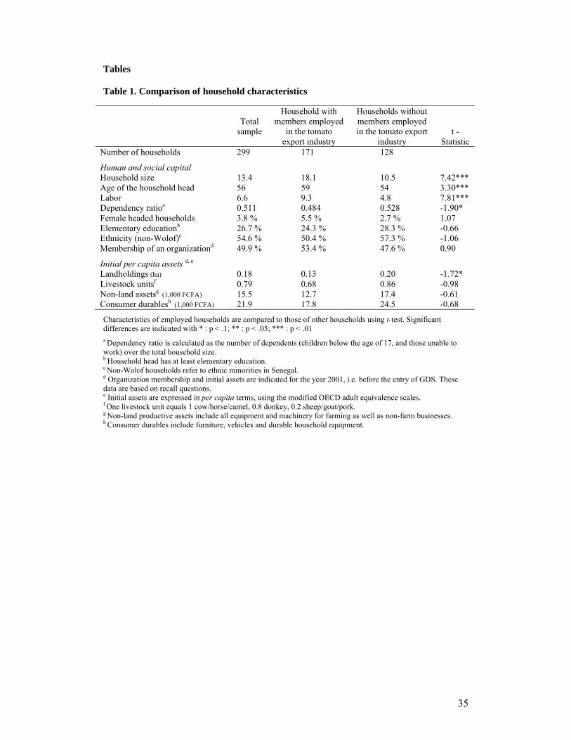
In Table 1 we compare the characteristics of households with one or more
members employed in the production and/or handling of tomatoes for export, and
households without such employment. The figures show that these two groups of
households differ substantially in certain household characteristics. Employees in the
tomato export industry come from significantly larger households, with an older
household head, significantly larger labor endowments and fewer dependents. There
is no disparity between the two groups of households in their level of education and
their ethnicity. Yet, households with employees in the tomato export industry initially
– in 2001, before GDS invested and started to recruit local households – had
significantly smaller landholdings. They also have slightly lower initial livestock and
non-land asset holdings, but none of these differences are significant at the 0.1 level.
In summary, this comparison suggests that employment in the tomato export industry
is not biased towards relatively better-off or more educated households; in contrast,
the employment is biased towards households with smaller landholdings. No major
entry constraints in the form of education or wealth seem to exist for entry into
employment in the tomato export sector.
Household Income
Total household income is calculated from the survey data for the 12-month
period prior to the survey (2005-2006) and using the modified OECD adult
equivalence scale for per capita measures. Comparing incomes for households with
member(s) employed in the tomato export industry and households without such
employment, we find that employment in the sector is associated with larger total and
17
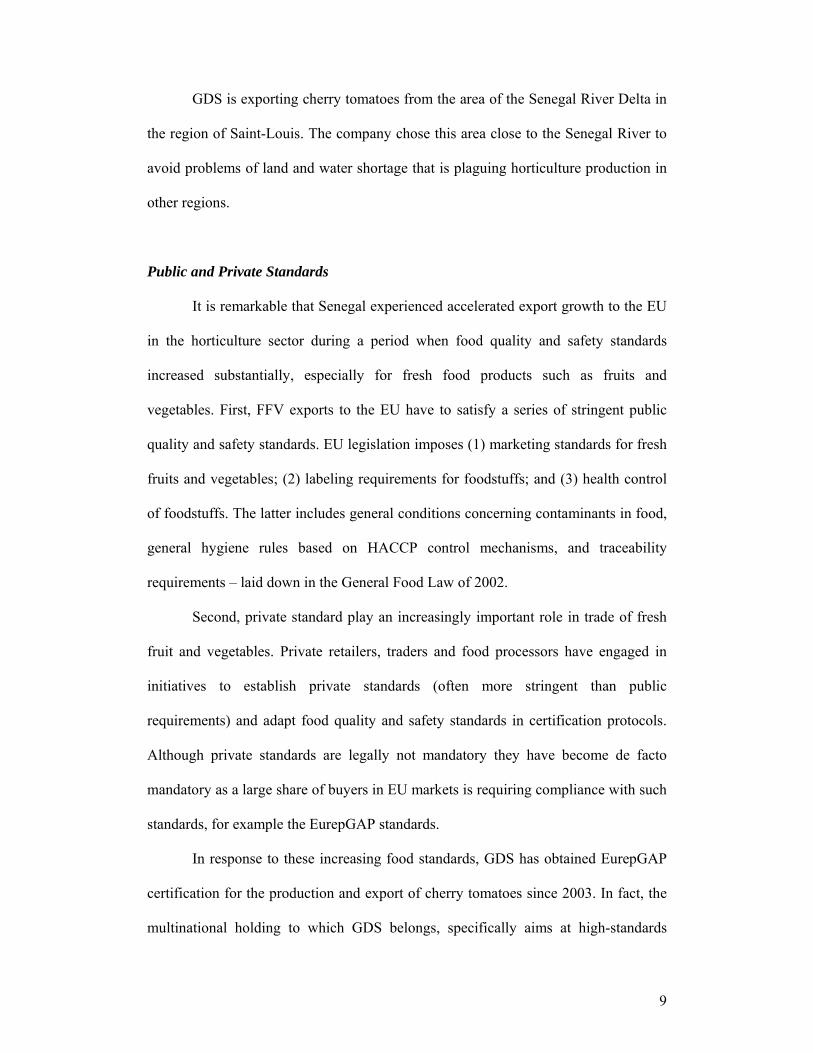
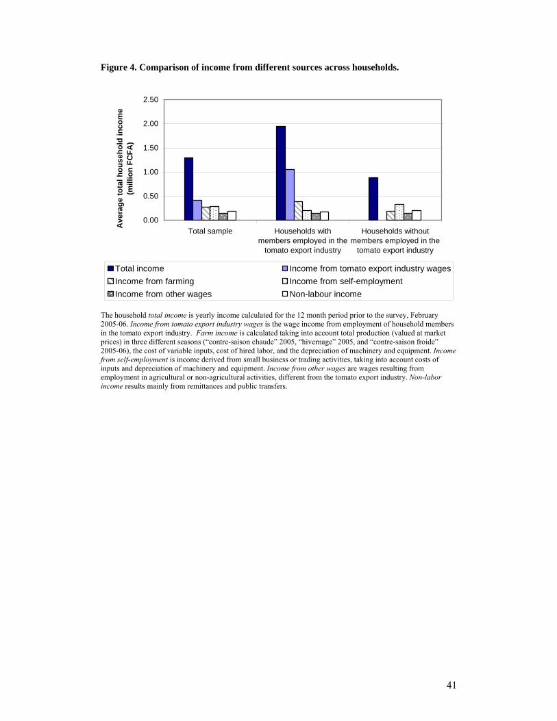
per capita incomes. Households with members employed in the tomato export
industry have an average income of 1.95 million FCFA. This is more than two times
larger than the average income of other households, which is 0.88 million FCFA
(Figure 4). Also in per capita terms these income differences remain large: 277,000
FCFA per capita for households with GDS employees versus 212,000 FCFA per
capita for other households – this is more than 30% higher.
The wages received from working on the fields and in the conditioning centre
of GDS add substantially to rural incomes. One third of total household income in the
survey region is derived from these wages (Figure 4). Looking only at those
households taking up this employment, this even increases to 54%. Hence, the tomato
export sector – despite the fact that its activities are very seasonal and associated
employment mostly temporarily – has become the main source of income in the
region. Nevertheless, most households continue to have diversified income portfolios
(Figure 4). Income sources include – apart from wages received from GDS (34%) –
farming (21%), self-employment (mostly small trading activities – 18%), other wages
(11%) and non-labor income (mostly remittances and public transfers – 16%).
Poverty Rates
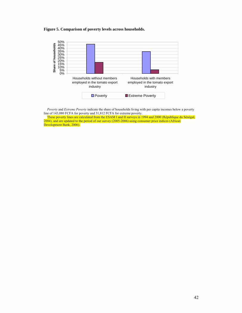
Based on household per capita incomes, we calculate the incidence of poverty
in the research area. We use a poverty line of 143,080 FCFA per capita for poverty
and 31,812 FCFA per capita for extreme poverty and calculate the share of
households living below these national rural poverty lines. The poverty lines are
calculated from the ESAM I and II surveys in 1994 and 2000 (République du Sénégal,
2004), and are updated to the period of our survey (2005-2006) using consumer price
indices (African Development Bank, 2006).
18
The incidence of poverty in the research area is 13% for extreme poverty and
42% for poverty, which is lower than the average national rural poverty rate of 58%
(Figure 5). Poverty is much lower among households that are employed in the tomato
export industry (35%), compared to those without such employment (46%). The same
is valid for extreme poverty: 6% compared to 18% (Figure 5). These are large and
important differences. Poverty is 11 percentage points – and extreme poverty 12
percentage points – lower among households with employment at GDS. These effects
appear especially remarkable since our earlier comparison indicated that employment
in GDS was not biased towards initially better-off households (see Table 1). Although
we cannot yet derive causal relations based on the descriptive analysis so far, the
figures suggest that the growth in tomato exports and associated employment have
lead to upwards rural income mobility and poverty reduction in the research region.
5. Econometric Analysis
The descriptive analysis in the previous section indicates that there is a
substantial difference in income across households and that this difference is
correlated with employment in the tomato export industry. However, to identify
whether we can attribute these differences to the causal impact of this employment,
we need more detailed econometric analysis. In this section we identify and describe
various econometric models to estimate the effect of employment in the tomato export
industry on household income, and present and discuss the results of the estimations.
5.1. Methodology
19
We are interested in estimating the effect of employment with GDS –
expressed by a treatment variable6 Ti – on household income Yi. Apart from the
treatment effect, income is determined by other relevant covariates represented by the
vector Xi, including household productive asset holdings and other characteristics that
may affect productivity and profits.
Yi = θ + α Ti + βXi + εi , ∀ i (1)
Difficulties may arise in estimating the effect of Ti on Yi because the treatment
variable Ti can be arbitrarily correlated with the error term or unobserved
heterogeneity. This may be the case as selection into employment in the tomato agro-
industry is likely to be non-random. The company-employer may select households
based on their location and certain characteristics. Indeed, GDS recruits daily laborers
through local village organizations7 and mobilizes trucks to pick-up laborers in nearby
and easily accessible villages. In addition, households may self-select into
employment, e.g. because they have relatively small landholdings and no other
employment opportunities.
We use two different sets of techniques to deal with the potential bias. In a
first set of models the problem is treated as an endogeneity problem where the partial
effect of the treatment variable depends only on observed exogenous variables.
Accordingly, we use simple OLS estimation and IV estimation to reveal the effect of
employment in the agro-industry on household income. In a second set of models, we
treat the unobserved heterogeneity as a sample selection problem arising from the fact
that household income without treatment is unobserved for treated unites (and vice
6 We will use techniques described in the literature on average treatment effect and therefore call our dummy variable of interest the treatment variable. The techniques described in this literature were initially applied to the impact evaluation of job training programs but have since known a wide application in development economics studies. 7 To recruit workers GDS is working with the so-called GIE – Groupement d’Interet Economique, village organizations – such as farmer unions and other business associations – who call together teams of laborers for daily labor on the fields or in the conditioning centre of GDS.
20
versa) and estimate the effect using propensity score matching techniques. We
describe the models in detail below.
OLS Estimation
In a first model we use the selection-on-observables method first described by
Heckman and Robb (1985). We estimate equation (1) using OLS estimation and
including a large set of covariates Xi, anticipating these can correct for unobserved
heterogeneity. The vector Xi includes the following covariates: the number of
laborers in the households and its square (Labor & Labor2), the cultivated area (Farm
size), the number of livestock units (Livestock), the value of non-land assets (Non-
land assets), the age of the household head (Age), a dummy variable for household
heads with at least primary education (Education), a dummy variable for households
belonging to an ethnic minority (non-Wolof) group (Ethnicity), and the distance from
the residence village to the nearest city Saint-Louis and its square (Distance &
Distance2).
Instrumental Variable Estimation
In a second model – the dummy endogenous variable model, first described by
Heckman (1978) – we estimate equation (2) using an instrumental variable estimation
technique to control for the endogeneity of treatment. We use a standard IV method in
which the probability of employment in the tomato export industry Prob(Ti) is
estimated in the first-stage probit model and the estimated probabilities used as an
instrumented covariate in the second-stage structural model:
Yi = θ + α Prob(Ti) + βXi + εi , ∀ i (2)
with Prob(Ti)= λ + γZi + μi , ∀ i
21
We use the same vector of covariates Xi as in the previous model. Yet, we estimate
the IV model twice with slightly different specifications of the vector Zi in the first-
stage probit model. In a first specification A, the vector Zi includes all covariates
potentially relevant for determining selection into treatment. On the one hand,
households may self-select into employment in the tomato agro-industry based on
their access to resources and their preferences. On the other hand, the company itself
can select or exclude potential workers based on their skills, access to resources, etc.
In addition, there might be some geographic selection because the company’s
transportation costs for searching for/picking up laborers increases in more distant and
more remote villages, or because workers’ travel cost increases with distance. For the
same reason, the company may prefer to recruit in larger villages with a larger
number of potential laborers. We also need to account for the fact that the company
recruits laborers through village organizations.
To account for all these potential sources of bias in the selection of employees
in the tomato export industry we include the following covariates in the vector Zi: the
number of laborers in the households (Labor), initial per capita landholdings (Land),
initial per capita livestock holdings (Livestock), initial per capita non-land assets
(Other assets), the age of the household head (Age), a dummy variable for household
heads with at least primary education (Education), a dummy variable for belonging to
an ethnic minority (non-Wolof) (Ethnicity), a dummy variable for initial household
membership of a professional organization (Organization), a dummy variable for
households living in a village along a paved road (Road), and the population size of
the village the household lives in and its square (Population and Population2).
Covariates referring to the initial situation are based on recall data for the year 2001,
before GDS started its investments in the region. Hence Zi includes a mixture of
22
covariates that are also incorporated in the vector Xi and covariates that are not. In a
second specification B, we use a subset of these covariates and include in Zi only
those covariates that have a significant effect (at the 0.1 level) in the probit model.
Propensity Score Matching Techniques
Treating the unobserved heterogeneity as a sample selection problem, we want
to estimate the effect of employment in the tomato export industry on household
income – the average treatment effect ATE – as the difference between the income
with treatment Y1 and the income without treatment Y0:
ATE = E(Y1 – Y0) (3)
The ATE can be consistently estimated using propensity score matching techniques,
as first described by Rosenbaum and Rubin (1983). This involves pairing treatment
and comparison units that are similar in terms of their observable characteristics and
calculating the ATE as a weighted average of the outcome difference between treated
and matched controls (Abadie and Imbens, 2002; Dehejia and Wahba, 2002; Imbens
2004; Wooldridge, 2002). We first estimate the propensity score as the conditional
probability of treatment Prob(Ti=1| Zi) using a probit model. For the probit model, we
use the same specifications A and B as described above in equation (2). Then
treatment units and control units are matched on the estimated propensity scores.
We use two different matching techniques: nearest neighbor matching (model
3) and kernel matching (model 4). The nearest neighbor matching method calculates
the ATE as the weighted average of the difference in outcomes of treated and matched
control units. We use single-nearest-neighbor matching, which according to Imbens
(2004) leads to the most credible inferences with the least bias. Matching is done with
replacement as to assure that each treatment unit is matched to the control unit with
23
the closest propensity score, which reduces bias (Dehejia and Wahba, 2002). The
kernel matching method computes the ATE as the average difference in outcome of
treated and matched control case, where the matched control case is obtained as the
kernel weighted average of nearest control unit outcomes. Kernel matching is
particularly suited for ATE estimation with small sample sizes – such as sample of
299 households – as each treated unit is compared to a whole set of near control units;
and hence more information is used leading to improved estimates. In both models 3
and 4, only observations in the common support region – where the propensity score
of the treated unit is not higher than the maximum or less than the minimum
propensity score of the control units – are used for calculating the ATE (Becker and
Ichino, 2005).
Finally, note that there are two main assumptions underlying the consistency
of propensity score matching techniques. First, the conditional independence
assumption denotes that conditional upon observable covariates, the receipt of
treatment is independent of the potential outcome with and without treatment (Dehejia
and Wahba, 2002; Imbens, 2004). This assumption is intrinsically non-testable
because the data are uninformative about the distribution of the untreated outcome for
treated units and vice versa (Ichino et al., 2006; Imbens, 2004). Yet, Ichino et al.
(2006) proposed a method for addressing robustness of matching estimators to failure
of this assumption. We use this method and simulate a binary confounder – as in
Ichino et al. (2006) we use a neutral confounder and a confounder calibrated to mimic
observable binary covariates in the model – that is used as additional matching factor.
The results (Annex 3) that the estimates with binary confounder differ by less than
20% from the baseline matching estimators of model 3 and 4; which indicates that the
propensity score matching techniques yield robust estimates of the ATE.

24
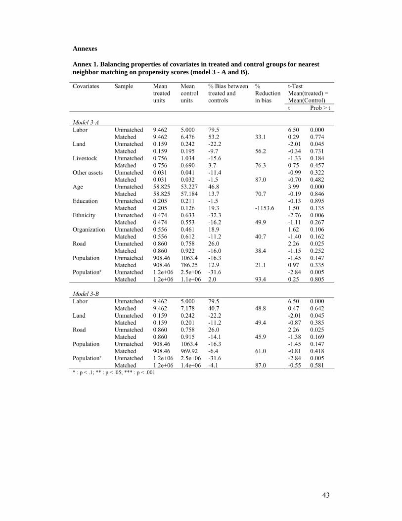
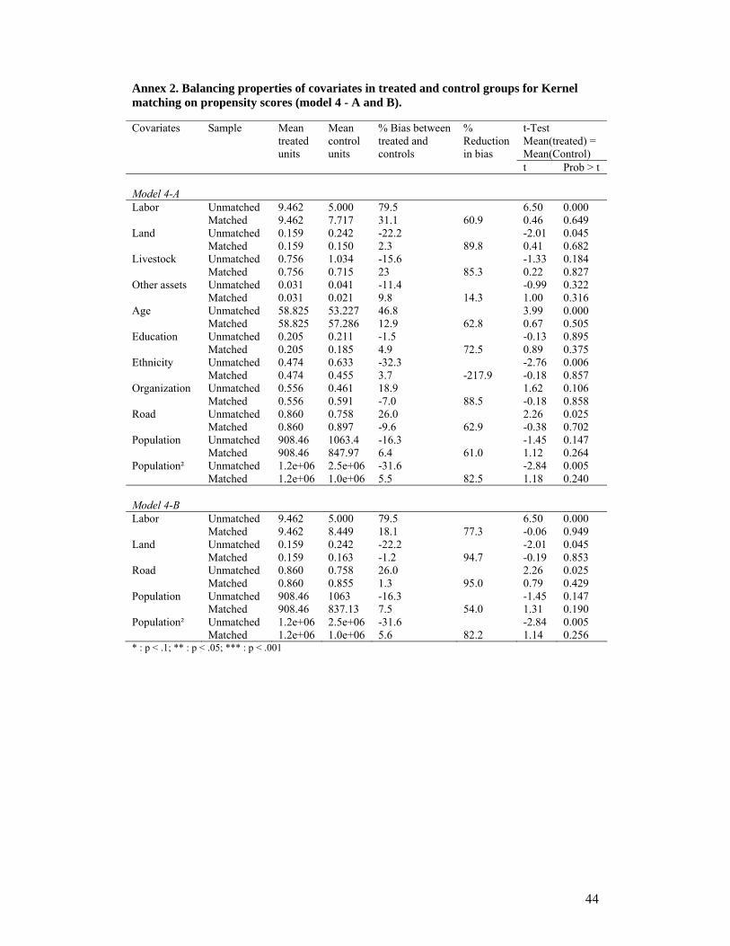
Second, propensity score matching requires balancing in the covariate
distribution between treated and untreated observations (Dehejia and Wahba, 2002;
Imbens, 2004). The balancing properties are addressed by testing for equality of
means between treated and matched controls for nearest neighbor matching in model
3 (Annex 1) and for kernel matching in model 4 (Annex 2). The results of these tests
show that there is no problem of unbalanced covariates in any of the models. For
many covariates there is a strong bias but matching eliminates this bias.
Robustness Tests and Interpretation
The use of four different econometric techniques to estimate the employment
effect already provides an important indication on the robustness of the estimated
results. In addition, we use two different specifications (model A and B) for the first
stage probit model, in the IV estimation (model 2) as well as in the propensity score
matching (model 3 and 4). This is done because the results of IV and ATE estimations
are known to be possibly sensitive to the choice of a proper set of covariates (Becker
and Ichino, 2005; Dehejia and Wahba, 2002; Imbens, 2004). Little is known about
strategic covariate choice (Imbens, 2004) and therefore we use two different
specifications to test the sensitivity of the results to covariate choice. As will be
documented in the next section, the estimated effects are extremely robust to the
various different techniques and the different specifications used in the models.
It should be noted that with the chosen approach we estimate the overall
impact of employment in the tomato export industry on household income. This
overall impact can stem from the direct effect of wages adding to household income
but also from indirect or secondary effects. These include for example the effect on
households’ own farm and other businesses from employee training in the tomato
25
industry or from increased investments in these activities with wages earned in the
tomato industry. In addition, there might be indirect or spillover effects for the rural
economy as a whole; for example because increased incomes might have price effects
in rural markets. Not all these effects are separately measurable with the data and
therefore we look at the overall effects without distinguishing between direct and
indirect effects.
5.2. Results and Discussion
Probability of Employment
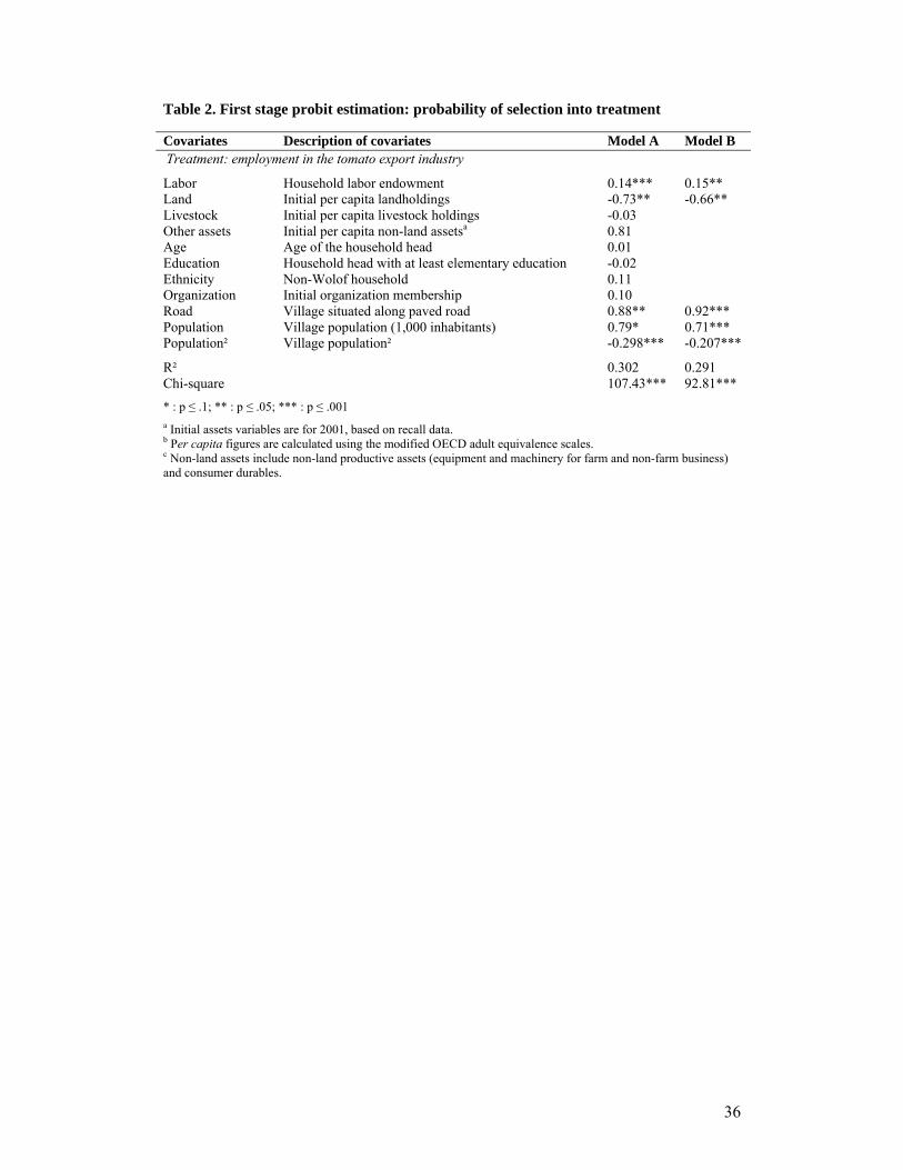
The results of the first stage probit models estimating the probability of
employment in the tomato export industry are presented in Table 2. The relatively
high R2 of the models show that the probability of employment is well explained by a
combination of household and village characteristics. In addition, the two different
specifications have identical results.
First, we find that households with a larger number of workers are more likely
to have members employed in the tomato export industry. Second, initial per capita
landholdings negatively affect the likelihood of having household members working
with GDS: for every additional ha of land the probability of employment in the
tomato export industry reduces with about 70 %. This indicates that households with
limited access to land and excess labor self-select into off-farm employment in the
agro-industry. Third, as expected, we find that households from larger villages and
from villages situated along a paved road have a higher likelihood of being employed.
This reflects the geographic selection resulting from transport costs, as mentioned in
the previous section. Fourth, education has no significant effect, indicating again that
education is not a constraint for entry into wage employment in the tomato sector.
26
Fifth, also other household characteristics such as initial livestock holdings, non-land
asset holdings, ethnicity or membership of a village organization have no significant
effect in the probit model. The latter result – on organization membership – is
somewhat surprising since it is known that GDS recruits laborers through village
organizations. The lack of an effect might be explained by the fact that villagers likely
seek membership of an organization to have access to GDS employment (rather than
having access to the employment because of their membership) and that hence initial
membership is not correlated with employment.
We can conclude that rather than being biased towards relatively better-off
and better educated households – as found by some studies on rural off-farm
opportunities in developing countries – wage employment in the tomato agro-industry
in Senegal is accessible for the households with low levels of education and assets.
Income Effects
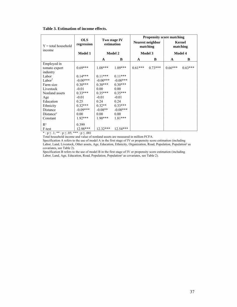
Table 3 presents the results of the four models estimating the treatment effect.
The main result of the analysis is that in all tested models we find a very significant
and strong positive impact of employment in the tomato export industry on total
household income. This result is consistent across the different estimation techniques
– OLS, IV estimation and propensity score matching techniques – and across the
different covariate specifications in the first-stage equation. This consistency suggests
a firm robustness of the results. The estimated effect varies between 0.61 and 1.09 and
is substantially larger in model 2 (IV estimation) compared to the other models. This
might result from the fact that the usual IV estimator is generally inconsistent for
27
binary treatment effects8 (Wooldridge, 2005). With propensity score matching
techniques we find more conservative – and probably more consistent and more
realistic (Wooldridge, 2005) – estimates of the income effect: between 0.61 and 0.73.
From this analysis, we can derive that households with members employed in
the tomato agro-industry have incomes that are between 610,000 FCFA to 730,000
FCFA higher than for households who do not take up such employment. This means
that these households have incomes that are 47% to 57% higher than the average
income in the region and 70 to 83% higher than those of households not employed in
the tomato sector. These are extremely large and important effects; especially since
entry into such employment is biased towards households with smaller land and
excess labor endowments.
Finally, the results of the second-stage income regression show that household
income is correlated with its labor, land and capital endowments. Labor has a
significant positive but decreasing effect on income. A larger farm size and more non-
land assets significantly increase household income. We find for example that an
increase of 1ha in the farm size increases household income with 300,000 FCFA. The
age and education of the household head have no significant effect on household
income. In addition, location with respect to the city Saint-Louis matters: being
located in a village 1 km further away from the city decreases household income with
80,000 to 90,000 FCFA.
6. Conclusions
8 The use of the IV estimation technique for an endogenous binary treatment is based on the simulation results found by Angrist (1991) that the usual IV estimator can provide a good estimate of the average treatment effect while in fact sufficient conditions for consistency of IV do not hold in the binary treatment case. However, the results of Angrist (1991) are a special case as he considers only a model without additional exogenous covariates (Wooldridge, 2005).
28
The impact of developing countries’ integration in global markets on poverty
and income inequality in these countries remains the subject of considerable
controversy. This paper has analyzed the household level effects – including income
mobility and poverty reduction – of increased foreign trade and investments in the
tomato sector in Senegal using a unique set of survey data. Our study shows that FDI
in the FFV sector and sharply expanded tomato exports has importantly benefitted
poor rural households through wage employment in the emerging agro-industry.
Using several different econometric techniques we find robust, significant and large
positive effects on income and poverty reduction.
Although, these conclusions are obviously drawn from the specific sector
which we studied and one should be careful to generalize, we believe that these
findings are particularly important. First, our case-study provides evidence at the
household level of a positive and direct link between globalization and poverty
reduction and thereby contributes to filling a gap in the empirical literature. Second,
our results challenge the general view in the literature that the gains from expanded
agri-food trade are concentrated with foreign investors and large food companies
while poor farmers are increasingly marginalized. Even with extreme levels of supply
base consolidation and complete vertical integration in the chains, there are important
benefits for the poor. Third, the results show that important benefits may come
through labor market effects rather then through product markets. This challenges the
implicit assumption underlying many empirical studies that export supply chains need
to integrate farm household as primary producers if agri-food trade is to benefit rural
incomes and poverty reduction. Fourth, related to this, we find that wage employment
in the agro-industry is accessible for resource-poor and less educated households,
29
indicating that rural off-farm employment creation might be an important poverty-
alleviation strategy.
Moreover, the case-study documented in this paper shows that pro-poor
globalization is possible, even in poor SSA countries, despite the many constraints.
This case-study on Senegalese tomato exports could add to the existing evidence of
high-standards export development in Sub Sahara Africa (e.g. in Kenya, South-Africa,
etc.) and thereby shift the balance from viewing standards as barriers to trade to the
standards-as-catalysts view.
Finally, it needs to be mentioned that the benefits from (foreign) investments
in the horticulture sector and expanded horticultural exports from Senegal are
concentrated in some regions and not yet shared equally all over the country. Yet, our
results indicate that there is scope for ongoing investments in other regions of the
country to result in expanded poverty-alleviating impacts.
30
References
Abadie, A. and Imbens, G., 2002. Simple and bias-corrected matching estimators for average treatment effects. NBER technical working paper No 283. Cambridge: National Bureau of Economic Research.
African Development Bank, 2006. Selected statistics on African countries (Vol. XXV). Tunis: Statistics Division, Development Research Department, African Development Bank.
Agénor R.P., 2004. Does Globalization Hurt the Poor? International Economics and Economic Policy, 1(1), 21-51
Aksoy, M.A. and Beghin, J.C., 2005. Global agricultural trade and developing countries. Washington DC: The World Bank.
Anderson, K. and Martin, W., 2005. Agricultural trade reform and the Doha Development Agenda. World Economy 28: 1301-1327.
Angrist, J.D., 1991. Instrumental variable estimation of average treatment effects in econometrics and epidemiology, National Bureau of Economic Research Technical Working Paper No. 115.
Barrett, C.B., Reardon T. and Webb P., 2001. Nonfarm income diversification and household livelihood strategies in rural Africa: Concepts, dynamics and policy implications. Food Policy 26: 315-31.
Barron, M.A. and Rello, F., 2000. The impact of the tomato agroindustry on the rural poor in Mexico. Agricultural Economics 23: 289-297.
Ben-David D., 1996. Trade and the rate of income convergence, Journal of International Economics 55: 229-34.
Becker, S. and Ichino A., 2005. Estimation of average treatment effects based on propensity scores. The Stata Journal 2: 358-377.
Bhagwati, J. and Srinivasan, T.N., 2002. Trade and poverty in the poor countries. American Economic Review 92: 180-183.
Blalock G. and Gertler P., 2008. Welfare gains from Foreign Direct Investment through technology transfer to local suppliers, Journal of International Economics 74(2): 402-421.
Borensztein, E., De Gregorio, J. and Lee, J-W., 1998. How does foreign direct investment affect economic growth?, Journal of International Economics, 45(1):115-135.
Carter, M. R, Barham, B. L., & Mesbah, D., 1996. Agricultural export booms and the rural poor in Chile, Guatemala and Paraguay. Latin American Research Review, 31(1), 33-65.
Choe J.I., 2003. Does Foreign Direct Investment and Domestic Investment Promote Economic Growth? Review of Development Economics 7(1): 44-57.
Choi C., 2006. Does foreign direct investment affect domestic income inequality? Applied Economics Letters 13: 811-814.
31
Colen. L., Maertens M., and J.F.M. Swinnen, 2008. Foreign Direct Investment as and Engine for Economic Growth and Human Development: A Review of the Arguments and Empirical Evidence. Working paper IAP VI/06.
Cooper R.N., 2002. Growth and inequality: The role of foreign and investment. In: Pleskovic, B. and Stern, N. (Eds.), Annual World Bank Conference on Development Economics 2001/2002, Washington DC. The World Bank.
Danielou, M. and Ravry, C., 2005. The rise of Ghana’s pineapple industry. Africa Region Working Paper Series 93. Washington DC: The World Bank, Africa Region.
Dehejia, R. H. and Wahba, S., 2002. Propensity score-matching methods for nonexperimental causal studies. The Review of Economics and Statistics 84: 151-161.
Dercon, S., 1998. Wealth, risk and activity choice: cattle in western Tanzania. Journal of Development Economics 55: 1-42.
Dollar, D. and Kraay, A., 2002. Growth is good for the poor. Journal of Economic Growth 7: 195-225.
Dollar, D. and Kraay, A., 2004. Trade, growth and poverty. Economic Journal 114: 22-49.
Dries, L., & Swinnen, J. F. M., 2004. Foreign Direct Investment, Vertical Integration and Local Suppliers: Evidence from the Polish Dairy Sector. World Development, 32(9), 1525-1544.
Farina, E.M.M.Q. and Reardon, T. ,2000. Agrifood grades and standards in the extended Mercosur: Their role in the changing agrifood system. American Journal of Agricultural Economics 82: 1170-1176.
Feenstra R.C. and Hanson G.H., 1997. Foreign Direct Investment and Relative Wages: Evidence from Mexico’s Maquiladoras, Journal of International Economics 42:371-393.
Fosu, A.K and A Mold, 2008. Gains from Trade: Implications for Labor Market Adjustment and Poverty Reduction in Africa, African Development Review/Revue Africaine de Développement 20(1): 20-48.
Frankel, J. and Romer, D., 1999. Does trade cause growth? American Economic Review 89: 379-399.
Garcia Martinez, M., and Poole, P., 2004. The development of private fresh produce safety standards: Implications for developing and Mediterranean exporting countries. Food Policy 29: 229-255.
Gibbon, P., 2003. Value-chain governance, public regulation and entry barriers in the global fresh fruit and vegetable chain into the EU. Development Policy Review 21: 615-625.
Gulati, A., Minot, N., Delgado, C. and Bora, S., 2007. Growth in high-value agriculture in Asia and the emergence of vertical links with farmers. In J.F.M. Swinnen (Ed.), Global supply chains, standards and the poor. Oxford: CABI Publishing.
Hansen H. and Rand J., 2006. On the Causal Links Between FDI and Growth in Developing Countries, The World Economy 29: 21–41.
32
Heckman, J.J., 1978. Dummy endogenous variables in a simultaneous equation system. Econometrica 46: 931-959.
Heckman, J.J. and Robb, R., 1985. Alternative methods for evaluating the impact of interventions: An overview. Journal of Econometrics 30: 239-267.
Henson, S. and S. Jaffee, 2008. Understanding Developing Country Strategic Responses to the Enhancement of Food Safety Standards. World Economy 31(4): 548-68.
Ichino, A., Mealli, F., and Nannicini, T., 2006. From temporary help jobs to permanent employment: What can we learn from matching estimators and their sensitivity? IZA Discussion Paper No 2149. Bonn: Institue for the Study of Labor.
Imbens, G., 2004. Nonparametric estimation of average treatment effects under exogeneity: a review. The review of Economics and Statistics 96: 4-29.
Irwin, D.A. and Tervio, M., 2002. Does trade raise income? Evidence from the twentieth century. Journal of International Economics 58: 1-18.
Jaffee, S., 2003. From challenge to opportunity: Transforming Kenya’s fresh vegetable trade in the context of emerging food safety and other standards in Europe. Agricultural and Rural Development Discussion Paper. Washington DC: The World Bank.
Jaffee, S. and Henson, S., 2004. Standards and agro-food exports from developing countries: Rebalancing the debate. World Bank Policy Research Working Paper No. 3348. Washington DC. The World Bank.
Jaffee, S. and Henson, S., 2005. Agro-food exports from developing countries: the challenges posed by standards. In Aksoy A.M. and Beghin J.C. (Eds.), Global agricultural trade and developing countries. Washington DC: The World Bank.
Jensen, N.M. and Rosas, G., 2007. Foreign direct investment and income inequality in Mexico, 1990-2000. International Organization 61(3): 467-487.
Key, N. and Runsten, D., 1999. Contract farming, smallholders, and rural development in Latin America: the organization of agroprocessing firms and the scale of outgrower production. World Development, 27: 381-401.
Kherralah, M., 2000. Access of smallholder farmers to the fruits and vegetables market in Kenya. Unpublished document. Washington DC: International Food Policy Research Institute.
Klein, M., Aaron, C. and Hadjimichael, B., 2001. Foreign direct investment and poverty reduction, World Bank Policy Research Working Paper No. 2613, Washinton DC. The World Bank
Kosack, S. and Tobin, J., 2006. Funding self-sustaining development: The role of aid, FDI and government in economic success, International Organization 60(1): 205-243.
Lindert, P. and Williamson, J., 2001. Does globalization make the world more unequal? NBER Working Papers No. 8228, National Bureau of Economic Research, Inc.
Lundberg, M. and Squire, L., 2003. The simultaneous evolution of growth and inequality. The Economic Journal 133 (487): 326-344.
33
Maertens, M. and Swinnen, J.F.M., 2007. Standards as barriers and catalysts for trade, growth and poverty reduction. Journal of International Agricultural Trade and Development 4: 47-61.
Maertens, M. and Swinnen, J.F.M., 2008. Trade, Standards and Poverty: Evidence from Senegal. World Development, doi:10.1016/j.worlddev.2008.04.006
McCulloh, N. and Ota, M., 2002. Export horticulture and poverty in Kenya, IDS Working Paper 174. Sussex: Institute for Development Studies.
Milanovic, B., 2002. Can we discern the effect of globalization on income distribution? Evidence from household budget surveys. World Bank Policy Research Working Paper No. 2876, Washington DC. The World Bank.
Minot, N. and Ngigi, M., 2004. Are horticultural exports a replicable success story? Evidence from Kenya and Côte d’Ivoire. EPTD/MTID discussion paper. Washington DC: IFPRI.
Minten, B., Randrianarison, L., Swinnen, J.F.M., 2008. Global retail chains and poor farmers: Evidence from Madagascar. World Development.
Nunnenkamp P., 2004. To what extent can foreign direct investment help achieve international development goals? The World Economy 27(5):657-677
Ravallion, M., 2006. Looking Beyond Averages in the Trade and Poverty Debate, World Development, 34(8): 1374-92.
Ravallion, M., 2001. “Growth, Inequality and Poverty: Looking Beyond Averages,” World Development, 29(11): 1803-1815.
Reardon, T., Codron, J.M., Busch, L., Bingen, J., and Harris, C., 1999. Global change in agrifood grades and standards: agribusiness strategic responses in developing countries. International Food and Agribusiness Management Review 2: 421-435.
Reardon, T., and Berdegué, J., 2002. The Rapid Rise of Supermarkets in Latin America: Challenges and Opportunities for Development. Development Policy Review, 20(4), 371-88.
Reardon, T., Timmer, P.C., Barrett, C., and Berdegué, J., 2003. The rise of supermarkets in Africa, Asia and Latin America. American Journal of Agricultural Economics 85: 1140-1146.
République du Sénégal, 2004. La pauvreté au Sénégal: De la dévaluation de 1994 à 2001-2002. Dakar : Ministère de l’Economie et des Finances, Direction de la Prévision et de la Statistique.
Rodriguez, F. and Rodrik, D., 2000. Trade policy and economic growth: A skeptic’s guide to the cross-national evidence. Cambridge and London: MIT Press.
Rosenbaum, P.R., and Rubin, D.B., 1983. The central role of propensity score in observational studies for causal effects. Biometrika 70: 41-55.
Srinivasan, T.N. and Bhagwati, J., 2001. Outward-orientation and development: Are revisionists right? In L. Deepak and R.H. Snape (Eds.), Trade, development and political economy: Essays in honour of Anne O. Krueger. New York: Palgrave.
Swinnen, J.F.M., 2005. When the market comes to you - or not. The dynamics of vertical co-ordination in agro-food chains in Europe and Central Asia. World Bank: Washington, D.C.
34
Swinnen, J.F.M. (ed.), 2007. Global supply chains. Standards and the poor. Oxford: CABI Publishing.
Swinnen J. and Maertens, M., 2007. Globalization, Privatization, and Vertical Coordination in Food Value Chains in Developing and Transition Countries. Agricultural Economics. 37 (2): 89-102.
Tsai, P., 1995. Foreign Direct Investment and Income Inequality: Further Evidence, World Development 23(3): 469-483.
UNCTAD, 2005. Economic Development in Africa. Rethinking the role of foreign direct investment, United Nations, New York.
Unnevehr, L.J., 2000. Food safety issues and fresh food product exports from LDCs. Agricultural Economics 23: 231-240.
Warning, M. and Key, N., 2002. The social performance and distributional impact of contract farming: An equilibrium analysis of the Arachide de Bouche Program in Senegal. World Development 30: 255-263.
Weatherspoon, D.D. and Reardon, T., 2003. The rise of supermarkets in Africa: Implications for agrifood systems and the rural poor. Development Policy Review 21: 333-356.
Wilson, J.S. and Abiola, V., 2003. Standards & global trade: a voice for Africa. Washington DC: The World Bank.
Winters, A.L., McCulloh, N. and McKay, A., 2004. Trade liberalization and poverty: the evidence so far. Journal of Economic Literature XLII: 72-115.
Wooldridge, J. M., 2002. Econometric Analysis of Cross Section and Panel Data. Cambridge: The MIT Press.
Wooldridge, J.M., 2005. Instrumental variables estimation of the average treatment effect in the correlated random coefficient model. Michigan: Department of Economics. Michigan State University.
World Bank, 2005. Food Safety and Agricultural Health Standards: Challenges and Opportunities for Developing Country Exports. Poverty Reduction and Economic Management Trade Unit and Agricultural and Rural Development Department, Report No 31207, Washington D.C.: The World Bank.
World Bank, 2008. World Development Report 2008: Agriculture for Development. World Bank, Washington D.C.
Xu B., 2000. Multinational enterprises, technology diffusion, and host country productivity growth, Journal of Development Economics 62(2): 477-493.
35
Tables Table 1. Comparison of household characteristics
Total sample
Household with members employed
in the tomato export industry
Households without members employed in the tomato export
industry t -
Statistic Number of households 299 171 128
Human and social capital Household size 13.4 18.1 10.5 7.42*** Age of the household head 56 59 54 3.30*** Labor 6.6 9.3 4.8 7.81*** Dependency ratioa 0.511 0.484 0.528 -1.90* Female headed households 3.8 % 5.5 % 2.7 % 1.07 Elementary educationb 26.7 % 24.3 % 28.3 % -0.66 Ethnicity (non-Wolof)c 54.6 % 50.4 % 57.3 % -1.06 Membership of an organizationd 49.9 % 53.4 % 47.6 % 0.90
Initial per capita assets d, e Landholdings (ha) 0.18 0.13 0.20 -1.72* Livestock unitsf 0.79 0.68 0.86 -0.98 Non-land assetsg (1,000 FCFA) 15.5 12.7 17.4 -0.61 Consumer durablesh (1,000 FCFA) 21.9 17.8 24.5 -0.68
Characteristics of employed households are compared to those of other households using t-test. Significant differences are indicated with * : p < .1; ** : p < .05; *** : p < .01 a Dependency ratio is calculated as the number of dependents (children below the age of 17, and those unable to work) over the total household size. b Household head has at least elementary education. c Non-Wolof households refer to ethnic minorities in Senegal. d Organization membership and initial assets are indicated for the year 2001, i.e. before the entry of GDS. These data are based on recall questions. e Initial assets are expressed in per capita terms, using the modified OECD adult equivalence scales. f One livestock unit equals 1 cow/horse/camel, 0.8 donkey, 0.2 sheep/goat/pork. g Non-land productive assets include all equipment and machinery for farming as well as non-farm businesses. h Consumer durables include furniture, vehicles and durable household equipment.
36
Table 2. First stage probit estimation: probability of selection into treatment Covariates Description of covariates Model A Model B Treatment: employment in the tomato export industry
Labor Household labor endowment 0.14*** 0.15** Land Initial per capita landholdings -0.73** -0.66** Livestock Initial per capita livestock holdings -0.03 Other assets Initial per capita non-land assetsa 0.81 Age Age of the household head 0.01 Education Household head with at least elementary education -0.02 Ethnicity Non-Wolof household 0.11 Organization Initial organization membership 0.10 Road Village situated along paved road 0.88** 0.92*** Population Village population (1,000 inhabitants) 0.79* 0.71*** Population² Village population² -0.298*** -0.207***
R² 0.302 0.291 Chi-square 107.43*** 92.81*** * : p ≤ .1; ** : p ≤ .05; *** : p ≤ .001 a Initial assets variables are for 2001, based on recall data. b Per capita figures are calculated using the modified OECD adult equivalence scales. c Non-land assets include non-land productive assets (equipment and machinery for farm and non-farm business) and consumer durables.
37
Table 3. Estimation of income effects.
Propensity score matching OLS
regression Two stage IV
estimation Nearest neighbor matching
Kernel matching
Model 1 Model 2 Model 3 Model 4
Y = total household income
A B A B A B Employed in tomato export industry
0.69*** 1.08*** 1.09*** 0.61*** 0.73*** 0.66*** 0.63***
Labor 0.14*** 0.11*** 0.11*** Labor2 -0.00*** -0.00*** -0.00*** Farm size 0.30*** 0.30*** 0.30*** Livestock -0.01 0.00 0.00 Nonland assets 0.33*** 0.35*** 0.35*** Age -0.01 -0.01 -0.01 Education 0.25 0.24 0.24 Ethnicity 0.32*** 0.32** 0.33*** Distance -0.09*** -0.08** -0.08*** Distance² 0.00 0.00 0.00 Constant 1.92*** 1.90*** 1.81***
R² 0.399 F-test 12.98*** 12.32*** 12.54*** * : p ≤ .1; ** : p ≤ .05; *** : p ≤ .001 Total household income and value of nonland assets are measured in million FCFA. Specification A refers to the use of model A in the first stage of IV or propensity score estimation (including Labor, Land, Livestock, Other assets, Age, Education, Ethnicity, Organization, Road, Population, Population² as covariates, see Table 2). Specification B refers to the use of model B in the first stage of IV or propensity score estimation (including Labor, Land, Age, Education, Road, Population, Population² as covariates, see Table 2).
38
Figures Figure 1. Horticulture exports (ton) from Senegal, 1997 – 2006.
0
5,000
10,000
15,000
20,000
25,000
30,000
1997 1998 1999 2000 2001 2002 2003 2004 2005 2006
Year
Expo
rt v
olum
e (to
n)
French bean Tomatoes Mango Other fruit & vegetables
Source: Eurotrans – Senegal
39
Figure 2. Research area: Rural communities Gandon and Ross Béthio selected for household survey. Senegal – Saint-Louis Source: IRD Cartographie
40
Figure 3. Household employment in tomato export industry, 2003-2006.
0%
10%
20%
30%
40%
50%
2003 2004 2005 2006Year
Shar
e of
hou
seho
lds
Gandon Ross Béthio Total
Employed households are households with one or several members working as an employee in the tomato export industry. Based on household survey recall data collected in 2006.
41
Figure 4. Comparison of income from different sources across households.
0.00
0.50
1.00
1.50
2.00
2.50
Total sample Households withmembers employed in the
tomato export industry
Households withoutmembers employed in the
tomato export industry
Ave
rage
tota
l hou
seho
ld in
com
e (m
illio
n FC
FA)
Total income Income from tomato export industry wagesIncome from farming Income from self-employmentIncome from other wages Non-labour income
The household total income is yearly income calculated for the 12 month period prior to the survey, February 2005-06. Income from tomato export industry wages is the wage income from employment of household members in the tomato export industry. Farm income is calculated taking into account total production (valued at market prices) in three different seasons (“contre-saison chaude” 2005, “hivernage” 2005, and “contre-saison froide” 2005-06), the cost of variable inputs, cost of hired labor, and the depreciation of machinery and equipment. Income from self-employment is income derived from small business or trading activities, taking into account costs of inputs and depreciation of machinery and equipment. Income from other wages are wages resulting from employment in agricultural or non-agricultural activities, different from the tomato export industry. Non-labor income results mainly from remittances and public transfers.
42
Figure 5. Comparison of poverty levels across households.
0%5%
10%15%20%25%30%35%40%45%50%
Households without membersemployed in the tomato export
industry
Households with membersemployed in the tomato export
industry
Shar
e of
hou
seho
lds
Poverty Extreme Poverty
Poverty and Extreme Poverty indicate the share of households living with per capita incomes below a poverty
line of 143,080 FCFA for poverty and 31,812 FCFA for extreme poverty. These poverty lines are calculated from the ESAM I and II surveys in 1994 and 2000 (République du Sénégal,
2004), and are updated to the period of our survey (2005-2006) using consumer price indices (African Development Bank, 2006).
43
Annexes Annex 1. Balancing properties of covariates in treated and control groups for nearest neighbor matching on propensity scores (model 3 - A and B). Covariates Sample Mean
treated units
Mean control units
% Bias between treated and controls
% Reduction in bias
t-Test Mean(treated) = Mean(Control)
t Prob > t Model 3-A Labor Unmatched 9.462 5.000 79.5 6.50 0.000 Matched 9.462 6.476 53.2 33.1 0.29 0.774 Land Unmatched 0.159 0.242 -22.2 -2.01 0.045 Matched 0.159 0.195 -9.7 56.2 -0.34 0.731 Livestock Unmatched 0.756 1.034 -15.6 -1.33 0.184 Matched 0.756 0.690 3.7 76.3 0.75 0.457 Other assets Unmatched 0.031 0.041 -11.4 -0.99 0.322 Matched 0.031 0.032 -1.5 87.0 -0.70 0.482 Age Unmatched 58.825 53.227 46.8 3.99 0.000 Matched 58.825 57.184 13.7 70.7 -0.19 0.846 Education Unmatched 0.205 0.211 -1.5 -0.13 0.895 Matched 0.205 0.126 19.3 -1153.6 1.50 0.135 Ethnicity Unmatched 0.474 0.633 -32.3 -2.76 0.006 Matched 0.474 0.553 -16.2 49.9 -1.11 0.267 Organization Unmatched 0.556 0.461 18.9 1.62 0.106 Matched 0.556 0.612 -11.2 40.7 -1.40 0.162 Road Unmatched 0.860 0.758 26.0 2.26 0.025 Matched 0.860 0.922 -16.0 38.4 -1.15 0.252 Population Unmatched 908.46 1063.4 -16.3 -1.45 0.147 Matched 908.46 786.25 12.9 21.1 0.97 0.335 Population² Unmatched 1.2e+06 2.5e+06 -31.6 -2.84 0.005 Matched 1.2e+06 1.1e+06 2.0 93.4 0.25 0.805 Model 3-B Labor Unmatched 9.462 5.000 79.5 6.50 0.000 Matched 9.462 7.178 40.7 48.8 0.47 0.642 Land Unmatched 0.159 0.242 -22.2 -2.01 0.045 Matched 0.159 0.201 -11.2 49.4 -0.87 0.385 Road Unmatched 0.860 0.758 26.0 2.26 0.025 Matched 0.860 0.915 -14.1 45.9 -1.38 0.169 Population Unmatched 908.46 1063.4 -16.3 -1.45 0.147 Matched 908.46 969.92 -6.4 61.0 -0.81 0.418 Population² Unmatched 1.2e+06 2.5e+06 -31.6 -2.84 0.005 Matched 1.2e+06 1.4e+06 -4.1 87.0 -0.55 0.581 * : p < .1; ** : p < .05; *** : p < .001
44
Annex 2. Balancing properties of covariates in treated and control groups for Kernel matching on propensity scores (model 4 - A and B). Covariates Sample Mean
treated units
Mean control units
% Bias between treated and controls
% Reduction in bias
t-Test Mean(treated) = Mean(Control)
t Prob > t Model 4-A Labor Unmatched 9.462 5.000 79.5 6.50 0.000 Matched 9.462 7.717 31.1 60.9 0.46 0.649 Land Unmatched 0.159 0.242 -22.2 -2.01 0.045 Matched 0.159 0.150 2.3 89.8 0.41 0.682 Livestock Unmatched 0.756 1.034 -15.6 -1.33 0.184 Matched 0.756 0.715 23 85.3 0.22 0.827 Other assets Unmatched 0.031 0.041 -11.4 -0.99 0.322 Matched 0.031 0.021 9.8 14.3 1.00 0.316 Age Unmatched 58.825 53.227 46.8 3.99 0.000 Matched 58.825 57.286 12.9 62.8 0.67 0.505 Education Unmatched 0.205 0.211 -1.5 -0.13 0.895 Matched 0.205 0.185 4.9 72.5 0.89 0.375 Ethnicity Unmatched 0.474 0.633 -32.3 -2.76 0.006 Matched 0.474 0.455 3.7 -217.9 -0.18 0.857 Organization Unmatched 0.556 0.461 18.9 1.62 0.106 Matched 0.556 0.591 -7.0 88.5 -0.18 0.858 Road Unmatched 0.860 0.758 26.0 2.26 0.025 Matched 0.860 0.897 -9.6 62.9 -0.38 0.702 Population Unmatched 908.46 1063.4 -16.3 -1.45 0.147 Matched 908.46 847.97 6.4 61.0 1.12 0.264 Population² Unmatched 1.2e+06 2.5e+06 -31.6 -2.84 0.005 Matched 1.2e+06 1.0e+06 5.5 82.5 1.18 0.240 Model 4-B Labor Unmatched 9.462 5.000 79.5 6.50 0.000 Matched 9.462 8.449 18.1 77.3 -0.06 0.949 Land Unmatched 0.159 0.242 -22.2 -2.01 0.045 Matched 0.159 0.163 -1.2 94.7 -0.19 0.853 Road Unmatched 0.860 0.758 26.0 2.26 0.025 Matched 0.860 0.855 1.3 95.0 0.79 0.429 Population Unmatched 908.46 1063 -16.3 -1.45 0.147 Matched 908.46 837.13 7.5 54.0 1.31 0.190 Population² Unmatched 1.2e+06 2.5e+06 -31.6 -2.84 0.005 Matched 1.2e+06 1.0e+06 5.6 82.2 1.14 0.256 * : p < .1; ** : p < .05; *** : p < .001
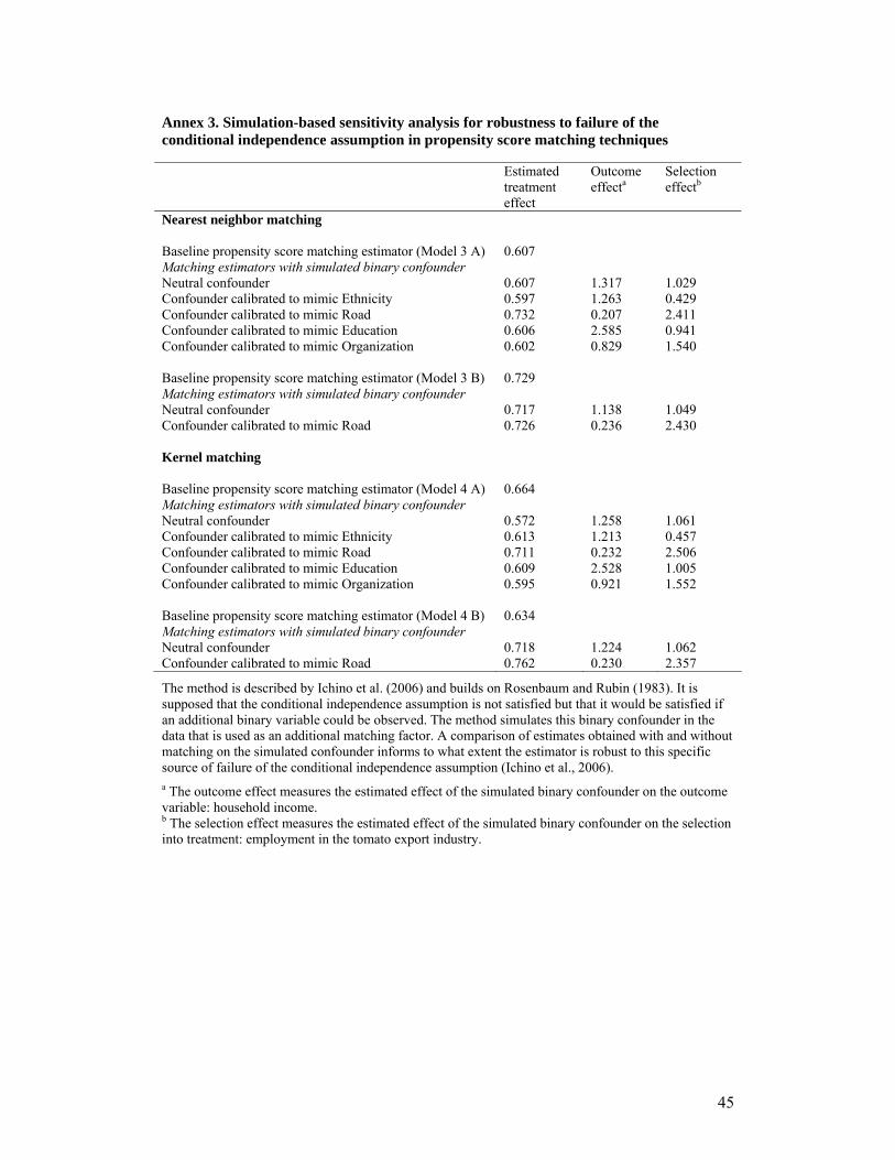
45
Annex 3. Simulation-based sensitivity analysis for robustness to failure of the conditional independence assumption in propensity score matching techniques
Estimated
treatment effect
Outcome effecta
Selection effectb
Nearest neighbor matching Baseline propensity score matching estimator (Model 3 A) 0.607 Matching estimators with simulated binary confounder Neutral confounder 0.607 1.317 1.029 Confounder calibrated to mimic Ethnicity 0.597 1.263 0.429 Confounder calibrated to mimic Road 0.732 0.207 2.411 Confounder calibrated to mimic Education 0.606 2.585 0.941 Confounder calibrated to mimic Organization 0.602 0.829 1.540 Baseline propensity score matching estimator (Model 3 B) 0.729 Matching estimators with simulated binary confounder Neutral confounder 0.717 1.138 1.049 Confounder calibrated to mimic Road 0.726 0.236 2.430 Kernel matching Baseline propensity score matching estimator (Model 4 A) 0.664 Matching estimators with simulated binary confounder Neutral confounder 0.572 1.258 1.061 Confounder calibrated to mimic Ethnicity 0.613 1.213 0.457 Confounder calibrated to mimic Road 0.711 0.232 2.506 Confounder calibrated to mimic Education 0.609 2.528 1.005 Confounder calibrated to mimic Organization 0.595 0.921 1.552 Baseline propensity score matching estimator (Model 4 B) 0.634 Matching estimators with simulated binary confounder Neutral confounder 0.718 1.224 1.062 Confounder calibrated to mimic Road 0.762 0.230 2.357
The method is described by Ichino et al. (2006) and builds on Rosenbaum and Rubin (1983). It is supposed that the conditional independence assumption is not satisfied but that it would be satisfied if an additional binary variable could be observed. The method simulates this binary confounder in the data that is used as an additional matching factor. A comparison of estimates obtained with and without matching on the simulated confounder informs to what extent the estimator is robust to this specific source of failure of the conditional independence assumption (Ichino et al., 2006). a The outcome effect measures the estimated effect of the simulated binary confounder on the outcome variable: household income. b The selection effect measures the estimated effect of the simulated binary confounder on the selection into treatment: employment in the tomato export industry.


